Long-Run E�ects of Competition on Solar Photovoltaic

Demand and Pricing∗

Bryan Bollinger†

Duke University

Kenneth Gillingham‡

Yale University

Stefan Lamp§

TSE

Preliminary Draft - April 2017

Abstract

The relationship between competition and economic outcomes is a �rst order question in eco-

nomics, with important implications for regulation and social welfare. This study presents

the results of a �eld experiment examining the impact of exogenously-varied competition

on equilibrium prices and quantities in the market for residential solar photovoltaic panels.

We alter the speci�cations of a large-scale behavioral intervention by allowing either one

or multiple �rms to operate through the program in randomly-allocated markets. Our �nd-

ings con�rm the classic result that an increase in competition lowers prices and increases

demand, both during the intervention and afterwards. The persistence of the e�ects in the

post-intervention period highlights the value of facilitating competition in behavioral inter-

ventions.

Keywords: pricing; imperfect competition; di�usion; new technology; energy policy.

JEL classi�cation codes: Q42, Q48, L13, L25, O33, O25.

∗The authors would like to thank the Connecticut Green Bank and SmartPower for their support. All errors are

solely the responsibility of the authors.

†Corresponding author: Fuqua School of Business, Duke University, 100 Fuqua Drive, Durham, NC 27708, phone:

919-660-7766, e-mail: bryan.bollinger@duke.edu.

‡School of Forestry & Environmental Studies, Department of Economics, School of Management, Yale University,

195 Prospect Street, New Haven, CT 06511, phone: 203-436-5465, e-mail: kenneth.gillingham@yale.edu.

§Toulouse School of Economics, Manufacture des Tabacs, 21 Alleé de Brienne, 31015 Toulouse Cedex 6, phone:

+33 561-12-2965, e-mail: stefan.lamp@tse-fr.eu.

1 Introduction

The study of price competition in imperfect markets has been a fundamental part of industrial

organization (IO) since Bertrand (1883).1

While early competition models have been rejected by

the data, recent advances in empirical IO led to the estimation of more complex structural models

reconciling theory and empirics. However, these models themselves often rely on a series of

assumptions that are not directly testable. On the other hand, the design of randomized �eld

experiments to analyze the impact of competition on market outcomes is usually not available to

the researcher due to ethical concerns.

In this paper we exploit exogenous variation in competition resulting from a large �eld ex-

periment (Solarize Connecticut, CT) to study the impact of competition on equilibrium prices

and quantities. The ‘Solarize’ program is a community-level behavioral intervention aimed at in-

creasing the adoption of residential solar photovoltaics (solar PV) systems. While in the standard

program municipalities choose a single solar PV installer, alternative treatment designs include

three or more installers. This unique program feature allows us to test for the impact of increased

competition directly. To the best of our knowledge, this is the �rst study to provide �eld evidence

for the e�ects of competition on equilibrium outcomes for a large investment good (solar PV) in

the non-development context.2

The public goods character of solar PV makes this a particularly

interesting market to study, as the analysis can provide important guidance to policymakers con-

cerning e�ective market design that increases the adoption of ‘green technologies’.

The Solarize campaigns have several key pillars. Treated municipalities choose a solar PV

installer with whom to collaborate throughout the campaign. In order to be selected, installers

submit bids with a discount group price that is o�ered to all consumers in that municipality dur-

ing the program. The intervention begins with a kick-o� event and involves roughly 20 weeks

of community outreach. The primary outreach is performed by volunteer resident ‘solar am-

bassadors’ who encourage their neighbors and other community members to adopt solar PV,

e�ectively providing a major nudge towards adoption (see Gillingham and Bollinger 2017, for

1The concept of competition in economics plays a fundamental part since Adam Smith. However, the explicit

and systematic analysis of competition started not before 1871 (Stigler 1957).

2Busso and Galiani (2014) randomize competition to test for the impact of increased competition on prices and

quantities in the retail sector in the Dominican Republic.

1

details). While the standard campaigns (‘Classic’) involve a single ‘focal installer’, in ‘Solarize

Choice’ (Choice), three installers get selected to participate in the campaign. ‘Solarize Online’

(Online), on the other hand, uses an Internet platform where a multitude of installers actively

bid for customers. As Solarize installers receive extraordinary attention during the program du-

ration, they end up with temporal market power.3

We exploit this exogenous increase in the

number of competitors to test for the e�ect of competition on equilibrium outcomes. As Solarize

campaigns have been rolled out in a consecutive fashion in several rounds, for each treatment

variation (Choice and Online), we have a set of municipalities that receive the Classic treatment.

Furthermore, we can compare the outcomes in the treated municipalities to a group of control

towns with similar observable characteristics that engage in green energy programs, but have

not been part of Solarize.4

We develop a stylized model to guide our empirical analysis. The two main e�ects of a Solarize

campaign are to increase demand and to decrease the customer acquisition costs that installers

face. These e�ects lead to shifts in both the demand and supply curves during the campaign.

After the campaign, the installer once again is responsible for its own customer acquisition and

the supply curve shifts back. In addition, demand falls in the post-period, but not necessarily

entirely back to the pre-campaign demand curve. For example, the installers may have picked

the low-hanging fruit of customers most excited about solar. If some harvesting occurred, we

expect post-campaign prices and quantities to be lower. In the case of several installers (Choice

and Online), the installers split the residual demand. The resultant equilibrium price is lower than

in Classic, and the quantity is higher due to the greater shift in the aggregate supply curve from

the focal installers. This leads to lower equilibrium post-Solarize prices than in Classic. Unlike in

Classic, with harvesting, total demand for both focal installers may not fall in the post-campaign

period due to this lower equilibrium price, although the installers are now splitting the market.

3Even though the number of active installers are fairly comparable in the pre-campaign period for the three

treatments, selecting a single installer in Classic resulted in an average market share of 89.9% during the �ve-month

campaign window in the �rst intervention period (round 3) and 68.3% in a second intervention (round 5).

4During the �rst intervention period, September 2013 - February 2014 (round 3) we count with 11 Classic towns

and 6 Choice municipalities. In the second intervention period, November 2014 - April 2015 (round 5), there are a

total of 7 Classic towns and 4 Online municipalities. Our control group, the Connecticut Green Energy Community

network consists of a total of 55 municipalities spread across the state.

2

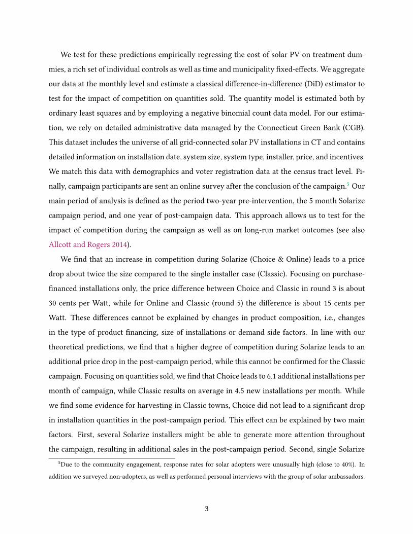
We test for these predictions empirically regressing the cost of solar PV on treatment dum-

mies, a rich set of individual controls as well as time and municipality �xed-e�ects. We aggregate

our data at the monthly level and estimate a classical di�erence-in-di�erence (DiD) estimator to

test for the impact of competition on quantities sold. The quantity model is estimated both by

ordinary least squares and by employing a negative binomial count data model. For our estima-

tion, we rely on detailed administrative data managed by the Connecticut Green Bank (CGB).

This dataset includes the universe of all grid-connected solar PV installations in CT and contains

detailed information on installation date, system size, system type, installer, price, and incentives.

We match this data with demographics and voter registration data at the census tract level. Fi-

nally, campaign participants are sent an online survey after the conclusion of the campaign.5

Our

main period of analysis is de�ned as the period two-year pre-intervention, the 5 month Solarize

campaign period, and one year of post-campaign data. This approach allows us to test for the

impact of competition during the campaign as well as on long-run market outcomes (see also

Allcott and Rogers 2014).

We �nd that an increase in competition during Solarize (Choice & Online) leads to a price

drop about twice the size compared to the single installer case (Classic). Focusing on purchase-

�nanced installations only, the price di�erence between Choice and Classic in round 3 is about

30 cents per Watt, while for Online and Classic (round 5) the di�erence is about 15 cents per

Watt. These di�erences cannot be explained by changes in product composition, i.e., changes

in the type of product �nancing, size of installations or demand side factors. In line with our

theoretical predictions, we �nd that a higher degree of competition during Solarize leads to an

additional price drop in the post-campaign period, while this cannot be con�rmed for the Classic

campaign. Focusing on quantities sold, we �nd that Choice leads to 6.1 additional installations per

month of campaign, while Classic results on average in 4.5 new installations per month. While

we �nd some evidence for harvesting in Classic towns, Choice did not lead to a signi�cant drop

in installation quantities in the post-campaign period. This e�ect can be explained by two main

factors. First, several Solarize installers might be able to generate more attention throughout

the campaign, resulting in additional sales in the post-campaign period. Second, single Solarize

5Due to the community engagement, response rates for solar adopters were unusually high (close to 40%). In

addition we surveyed non-adopters, as well as performed personal interviews with the group of solar ambassadors.

3

installers might be faced with capacity constraints and they might be unable to meet demand in

a timely manner in the post-period. The quantity response in Online are smaller than in Classic

(3.2 installations versus 5.5 installations respectively), which can be explained by demand side

factors.6

The overall market in round 5 has expanded importantly with the entry of the largest

solar energy service provider in the United States, SolarCity, and the provision of new type of

product �nancing.

We perform a series of robustness checks concerning our main results. In particular, we limit

our sample to cash-purchased installations only.7

We provide additional robustness checks for

the impact of focal installers as well as the main economic speci�cation. Finally, we experiment

regarding pre- and post-periods and concerning the group of included control municipalities. Our

main results are robust to these robustness checks. We further con�rm the signi�cance of our

�ndings using small sample inference (both random inference and the wild cluster bootstrap).

This paper makes two important contributions to the literature. First, taking advantage of a

large �eld experiment (Harrison and List 2004), we exploit the resulting local market power to test

for the impact of competition on equilibrium prices and quantities under di�erent settings. To the

best of our knowledge this is the �rst attempt to answer this classical question in economics in

the non-development context, relying on detailed administrative data. Second, as solar PV panels

are heavily subsidized, our study makes an important policy contribution, pointing towards the

role of supply side market power when it comes to technology di�usion.8

E�ective market design

that aims at increasing competition will lead to lower equilibrium prices and higher quantities and

hence will result in larger adoption of solar panels with bene�ts for greenhouse gas abatement.

The paper is structured as follows. The next section frames the papers contribution within the

existing literature. Section 3 introduces on the Solarize campaigns, before Section 4 elaborates

on the theoretical model. Section 5 describes the empirical setting and the design of the �eld

experiment, while Section 6 introduces the main regression model. Section 7 presents the main

6In Online, we �nd a larger share of potential customers that do not sign a purchase contract. Choice overload

and missing trust in the Internet platform are potential reasons for the lower sales conversion.

7The cost information for leasing products as well as loan-�nanced installations might contain measurement

errors as this information cannot be perfectly observed by the CT Green Bank.

8Evidence from post-campaign surveys point to the price as the most important factor in�uencing the solar

purchase decision.

4

results. Finally, Section 8 concludes.

2 Literature

This study relates to several strands of literature. The paper tests for classic IO theory and the

impact of market structure on equilibrium outcomes (Tirole 1988, Geroski 1995). Recent advances

in empirical IO (Einav and Levin 2010) led to the estimation of structural models of competition

(Bresnahan and Reiss 1991) in distinct industries; for example airlines (Berry 1992, Goolsbee and

Syverson 2008), car and car rentals (Bresnahan and Reiss 1990, Singh and Zhu 2008), and super-

markets (Jia 2008, Holmes 2011). Other studies rely on experimental data to uncover the impact

of competition on market outcomes (Dufwenberg and Gneezy 2000, Aghion, Bechtold, Cassar,

and Herz 2014). In contrast, the present paper relies on exogenous variation induced by a �eld

experiment to test for the equilibrium impacts of market concentration. The paper closest related

to our approach is Busso and Galiani (2014) that test for the impact of increased competition on

market outcomes relying on random variation from the implementation of a conditional cash

transfer program in the Dominican Republic. They �nd that six months after the intervention,

product prices in the treated areas had decreased by about 6%, while product quality and service

quality was not a�ected by the entry of new competitors.

In a broader sense the present study also relates to the growing literature in �eld experiments

in economics and behavioral policies in energy markets (see for example Allcott and Mullainathan

2010, Allcott and Rogers 2014). Other studies that analyze the impact of Solarize interventions

are Gillingham and Bollinger (2017) and Bollinger, Gillingham, and Tsvetanov (2016).

3 Solarize Connecticut

The Solarize CT program is a joint e�ort between a state agency, the Connecticut Green Bank

(CGB), and a non-pro�t marketing �rm, SmartPower. The �rst critical component to the Solarize

program is the selection of a focal installer. Solarize campaigns are usually built around one

trusted installer that collaborates with the volunteers and the non-pro�t in the implementation

of the town events.

5

The second major component to the Solarize program is the use of volunteer promoters or

ambassadors to provide information to their community about solar PV. There is growing evi-

dence on the e�ectiveness of promoters or ambassadors in driving social learning and in�uenc-

ing behavior (Kremer, Miguel, Mullainathan, Null, and Zwane 2011, Vasilaky and Leonard 2011,

BenYishay and Mobarak 2014, Ashraf, Bandiera, and Jack 2015, Kraft-Todd, Bollinger, Gillingham,

Lamp, and Rand 2017).

The third component is the focus on community-based recruitment. In Solarize, this consists

of mailings signed by the ambassadors, open houses to provide information about panels, tabling

at events, banners over key roads, ads in the local newspaper, and even individual phone calls by

the ambassadors to neighbors who have expressed interest.9

Finally, a major component is the group pricing discount o�ered to the entire community

based on the number of contracts signed. This provides an incentive for early adopters to con-

vince others to adopt and to let everyone know how many people in the community have adopted.

With the group pricing comes a limited deal duration for the campaign. The limited time frame

may provide a motivational reward e�ect (Du�o and Saez 2003), for the price discount would be

expected to be unavailable after the campaign. Thus, the program is designed as a package that

draws upon previous evidence on the e�ectiveness of social norm-based information provision,

the use of ambassadors to provide information, social pressure, prosocial appeals, goal setting,

and motivational reward e�ects for encouraging prosocial behavior. A more detailed description

on the Solarize program can be found in Gillingham and Bollinger (2017). The standard timeline

for a Solarize ‘Classic’ is as follows:

1. CGB and SmartPower inform municipalities about the program and encourage town leaders

to submit an application to take part in the program.

2. CGB and SmartPower select municipalities from those that apply by the deadline.

3. Municipalities issue a request for group discount bids from solar PV installers for each

municipality.

9Jacobsen, Kotchen, and Clendenning (2013) use non-experimental data to show that a community-based recruit-

ment campaign can increase the uptake of green electricity using some (but not all) of these approaches.

6

4. Municipalities choose a single installer, with guidance from CGB and SmartPower.

5. CGB and SmartPower recruit volunteer “solar ambassadors.”

6. A kicko� event begins a ∼20-week campaign featuring workshops, open-houses, local events,

etc. coordinated by SmartPower, CGB, the installer, and ambassadors.

7. Consumers that request them receive site visits and if the site is viable, the consumer may

choose to install solar PV.

8. After the campaign is over, the installations occur.

To study the role of competition directly, we experimentally varied the number of installers

selected to work within the campaign framework. Most installations during the campaign happen

through the campaign, so using a large scale behavioral intervention is what enabled us to directly

manipulate the competitive environment. All leads generated through the Solarize campaign

were shared with all of the installers.

3.1 Installer Selection

3.2 Experimental Setting

With the support of the CGB, The John Merck Fund, The Putnam Foundation, and a grant from

the U.S. Department of Energy, six rounds of Solarize CT have been run. Each of the rounds

included Solarize Classic campaigns, but in two of the rounds–the third and �fth–we experi-

mented with two additional treatments. In the �rst �eld experiment, we examined the impact

of campaigns with more than one focal installer on the price and quantity of solar installations

during the campaign and in the post-campaign period. Speci�cally, during round 3 (R3) we ran-

domly assigned towns to either be in the single focal installer ‘Classic’ version of Solarize, or the

‘Choice’ version, that chooses up to three installers per participating municipality. A total of 11

towns were assigned to the Classic program, while 6 towns received the Choice treatment. The

Classic and Choice campaigns started with a time lag of up to two month due to implementation

constraints.

7

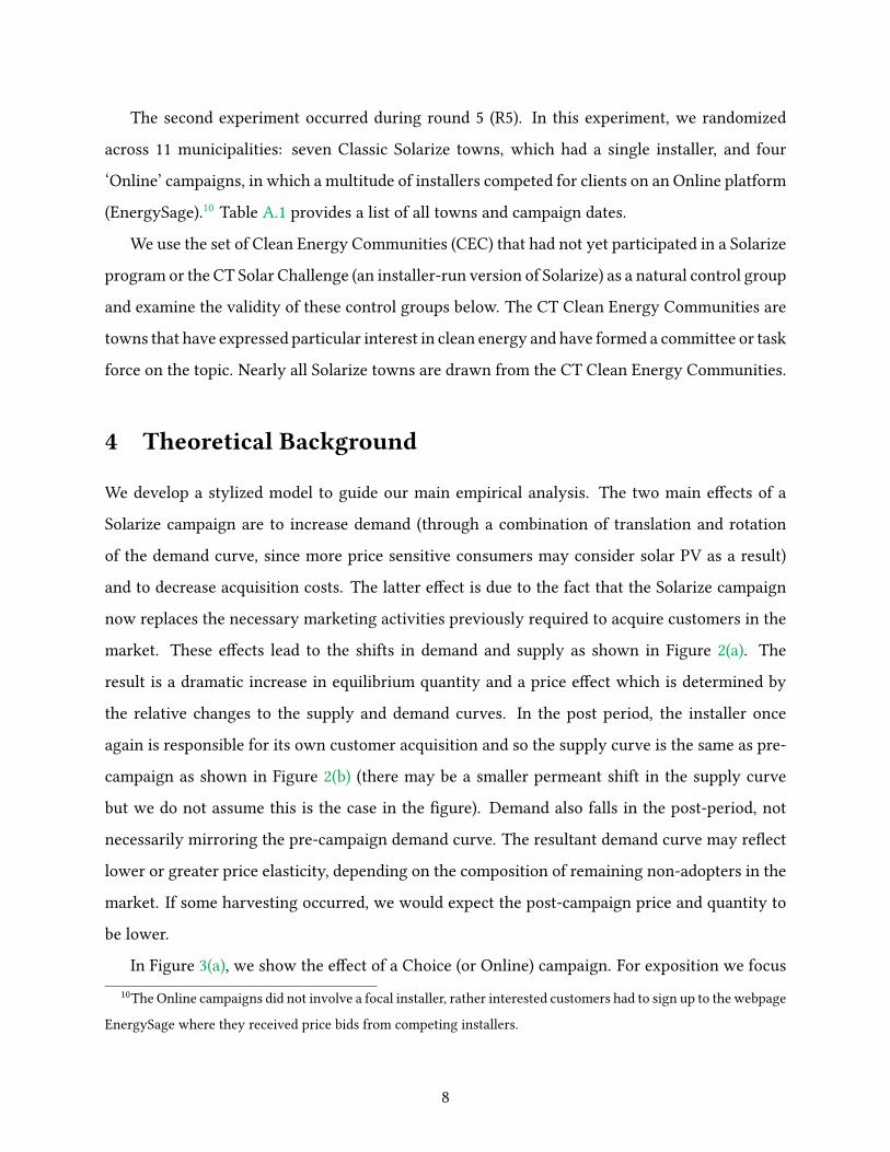
The second experiment occurred during round 5 (R5). In this experiment, we randomized

across 11 municipalities: seven Classic Solarize towns, which had a single installer, and four

‘Online’ campaigns, in which a multitude of installers competed for clients on an Online platform

(EnergySage).10

Table A.1 provides a list of all towns and campaign dates.

We use the set of Clean Energy Communities (CEC) that had not yet participated in a Solarize

program or the CT Solar Challenge (an installer-run version of Solarize) as a natural control group

and examine the validity of these control groups below. The CT Clean Energy Communities are

towns that have expressed particular interest in clean energy and have formed a committee or task

force on the topic. Nearly all Solarize towns are drawn from the CT Clean Energy Communities.

4 Theoretical Background

We develop a stylized model to guide our main empirical analysis. The two main e�ects of a

Solarize campaign are to increase demand (through a combination of translation and rotation

of the demand curve, since more price sensitive consumers may consider solar PV as a result)

and to decrease acquisition costs. The latter e�ect is due to the fact that the Solarize campaign

now replaces the necessary marketing activities previously required to acquire customers in the

market. These e�ects lead to the shifts in demand and supply as shown in Figure 2(a). The

result is a dramatic increase in equilibrium quantity and a price e�ect which is determined by

the relative changes to the supply and demand curves. In the post period, the installer once

again is responsible for its own customer acquisition and so the supply curve is the same as pre-

campaign as shown in Figure 2(b) (there may be a smaller permeant shift in the supply curve

but we do not assume this is the case in the �gure). Demand also falls in the post-period, not

necessarily mirroring the pre-campaign demand curve. The resultant demand curve may re�ect

lower or greater price elasticity, depending on the composition of remaining non-adopters in the

market. If some harvesting occurred, we would expect the post-campaign price and quantity to

be lower.

In Figure 3(a), we show the e�ect of a Choice (or Online) campaign. For exposition we focus

10The Online campaigns did not involve a focal installer, rather interested customers had to sign up to the webpage

EnergySage where they received price bids from competing installers.

8

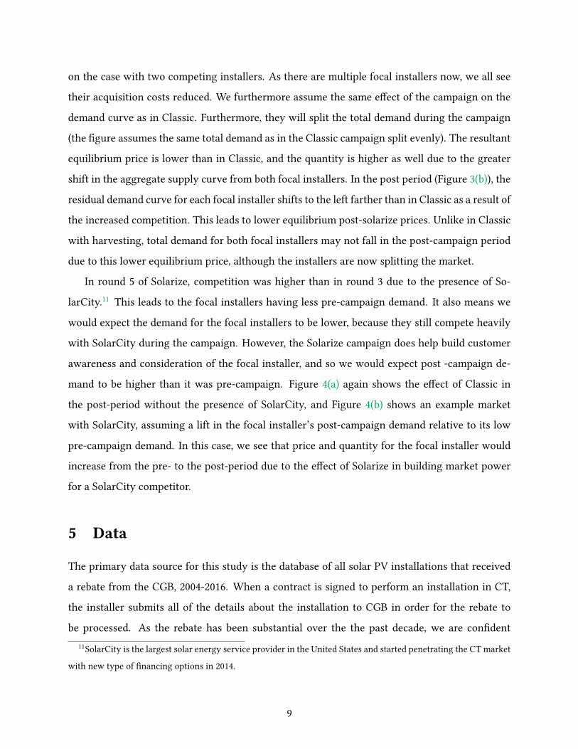
on the case with two competing installers. As there are multiple focal installers now, we all see

their acquisition costs reduced. We furthermore assume the same e�ect of the campaign on the

demand curve as in Classic. Furthermore, they will split the total demand during the campaign

(the �gure assumes the same total demand as in the Classic campaign split evenly). The resultant

equilibrium price is lower than in Classic, and the quantity is higher as well due to the greater

shift in the aggregate supply curve from both focal installers. In the post period (Figure 3(b)), the

residual demand curve for each focal installer shifts to the left farther than in Classic as a result of

the increased competition. This leads to lower equilibrium post-solarize prices. Unlike in Classic

with harvesting, total demand for both focal installers may not fall in the post-campaign period

due to this lower equilibrium price, although the installers are now splitting the market.

In round 5 of Solarize, competition was higher than in round 3 due to the presence of So-

larCity.11

This leads to the focal installers having less pre-campaign demand. It also means we

would expect the demand for the focal installers to be lower, because they still compete heavily

with SolarCity during the campaign. However, the Solarize campaign does help build customer

awareness and consideration of the focal installer, and so we would expect post -campaign de-

mand to be higher than it was pre-campaign. Figure 4(a) again shows the e�ect of Classic in

the post-period without the presence of SolarCity, and Figure 4(b) shows an example market

with SolarCity, assuming a lift in the focal installer’s post-campaign demand relative to its low

pre-campaign demand. In this case, we see that price and quantity for the focal installer would

increase from the pre- to the post-period due to the e�ect of Solarize in building market power

for a SolarCity competitor.

5 Data

The primary data source for this study is the database of all solar PV installations that received

a rebate from the CGB, 2004-2016. When a contract is signed to perform an installation in CT,

the installer submits all of the details about the installation to CGB in order for the rebate to

be processed. As the rebate has been substantial over the the past decade, we are con�dent

11SolarCity is the largest solar energy service provider in the United States and started penetrating the CT market

with new type of �nancing options in 2014.

9

that nearly all, if not all, solar PV installations in CT are included in the database.12

For each

installation the dataset contains the address of the installation, the date the contract was approved

by CGB, the date the installation was completed, the size of the installation, the pre-incentive

price, the incentive paid, whether the installation is third party-owned (e.g. solar lease or power-

purchase agreement), and additional system characteristics.

The secondary data source for this study is the U.S. Census Bureau’s 2009-2013 American

Community Survey, which includes demographic data at the municipality level. Further, we

include voter registration data at the municipality level from the CT Secretary of State (SOTS).

These data include the number of active and inactive registered voters in each political party, as

well as total voter registration (SOTS 2015).

We standardize the time period that we include in our analysis relative to the Solarize cam-

paign starting dates. For each campaign, we consider 24 month pre Solarize, the �ve month

Solarize campaign, and 12 month post campaign period. This approach allows us to compare the

treatment e�ects across campaigns relative to the Solarize interventions. For round 3 we consider

the full set of untreated clean energy communities as control towns. For round 5, we exclude the

10 largest towns, resulting in 45 control municipalities. This adjustment ensures that we are in-

deed comparing similar towns as treatment towns in later rounds have been slightly smaller. As

robustness, we verify that the choice of control towns does not impact our main results.

Town demographics for treatment and control groups one year prior to the Solarize interven-

tion are presented in Tables A.2 and A.3. The tables show that the distribution of key demographic

variables across treatment and control towns is indeed very similar.13

On the other hand, R3 treat-

ment towns had a larger mean and variability in mean cost and number of solar installations. In

order to contrast these �gures with price and quantity evolution, Figure A.1 shows the cumula-

tive uptake of installations as well as the mean prices (third-party owned installations excluded)

for the entire sample period in the three groups. Both treatment groups as well as the control

group have parallel pre-treatment trends.14

The appendix (Figure A.2) also presents histograms

12The only exception would be in three small municipal utility regions: Wallingford, Norwich, and Bozrah. We

expect that there are few installations in these areas.

13Statistical di�erences for key demographics can be only found for household income in Table A.2, and for the

share of homeowners and number of registered republican voters in Table A.3.

14In line with the visual inspection of the pre-treatment trends, we test for equal means of the �rst-di�erences

10

of the main dependent variables.

6 Empirical Strategy

6.1 Identi�cation

Using the exogenous change in the number of selected Solarize installers leads to important ex-

perimental variation in local and temporal market power. Table 1 provides evidence on the av-

erage market concentration and the number of active installers per municipality in �ve-month

intervals relative to the Solarize campaign timing. Focusing �rst on the period ‘during Solarize’,

we �nd that both Choice and Online lead to a signi�cant increase in active installers per town

relative to the Classic campaigns. This is in line with the experimental design, allowing for a

larger number of selected installers. Interestingly, we also see that the number of active installers

remains higher in the �ve-month period posterior to the policy intervention.

In order to grasp di�erences in market concentration, we look at the means of the normalized

Her�ndahl-Hirschman Index (HHI) in the same time periods. While Choice and Classic munic-

ipalities show a very similar market concentration in the pre-period (panel a), the single focal

installer in Classic leads to important increase in temporal market power (HHI of .63 compared

with .185 in Choice towns). The fact that in the post period Choice towns have more active in-

stallers leads to a lower market concentration index. R5 reveals slightly di�erent numbers. As the

overall market has matured importantly in 2014-15, we see a larger number of active installers

to begin with. Yet, similar to the case of Choice, Online leads to a signi�cant increase in the

number of active installers during the campaign. This results in a lower market concentration

compared to Classic. On the other hand, the market concentration indices in the post-period are

very similar for Online and Classic.

one year prior to Solarize and do not �nd evidence for statistic di�erences between the groups.

11

6.2 Price regression

To quantify the equilibrium impact of increasing competition, we estimate the following regres-

sion model based on individual data.

Priceimt = α+ δTmt + γPmt + βX + θm +ψt + εimt (1)

where Priceimt represents the price ($ per kilowatt) of solar installation i, in municipalitym,

at time period t. The regression includes municipality and month �xed-e�ects (FE) to account

for both time-invariant di�erences across municipalities and aggregate shocks to the CT solar

market. The control vector X includes observable characteristics of the solar installations such as

system size, type of system mounting and system �nancing.15

All standard errors are clustered

at municipality level, in order to account for error correlation within the same municipality over

time.

Our main coe�cients of interest are δ, which measures the treatment e�ect during the Solar-

ize interventions, and γ, which captures the di�erences in the post-Solarize period. We include

individual dummies for Choice and Classic in R3 and Online and Classic in R5 and estimate equa-

tion (1) for each round separately. We are interested in comparing the treatment e�ects and

post-treatment e�ects for Choice and Classic in the R3 regression as well as Online and Classic

in R5.

To better study the adjustment dynamics, we estimate a variation of (1). Using an event

study design (similar to Gallagher 2014), we introduce a full set of time dummies that is allowed

to vary by group (Classic, Choice, Control) and estimate the price impact relative to the Solar-

ize intervention.16

All results are relative to the two-month period pre-intervention.17

. Besides,

these alteration, the regression model contains all additional variables that have been used in

speci�cation (1).

15For robustness, we experiment with di�erent time �xed-e�ects (quarterly, annual combined with monthly dum-

mies). The main �ndings are robust to the choice of FE.

16As there are certain month with zero installations, we include one separate dummy for each two-month interval.

Moreover, as there have been few installations in the �rst months of our sample, we group these early installations

(24 month to 13 month prior to the campaigns) into a single dummy.

17This category is omitted from the regression.

12

6.3 Quantity regression

An additional outcome of interest are the equilibrium quantities sold in each market. For this pur-

pose we collapse our data at the municipality-month level and estimate a di�erence-in-di�erence

model:

Instmt = α+ δTmt ++γPmt + βX + θm +ψt + εmt (2)

where Instmt is the total number of new solar installations in municipality m, at time t. As

in (1), the model includes both municipality and month �xed-e�ects (FE). Our main interest lies

in the comparison of treatment (δ) and post-treatment (γ) coe�cients. To better understand the

dynamics, we follow the same event study design approach as outlined above. Moreover, as the

main dependent variable in (2) is count data, we estimate the model both by ordinary least squares

and by �tting a negative binomial count data regression.

7 E�ect of Competition on Equilibrium Outcomes

7.1 Descriptive evidence

First, descriptive evidence of the heterogeneous impact of distinct Solarize interventions on sys-

tem prices are given by Figure 4 that shows the mean price of solar installations by type of sys-

tem �nancing. Solar installations are either purchased, �nanced though a loan, leased through

an installer agreement or installed on basis of a third-party ownership, mainly so-called power

purchasing agreements (PPAs). As the type of �nancing can have an important impact on the cost

per Watt of a solar installation, Figure 4 compares average prices by type of �nancing. The �gure

shows the average price as well as standard deviation for R3 (Choice vs. Classic vs. Control) and

R5 (Online vs. Classic vs. Control) in �ve-month intervals relative to the Solarize campaign. Panel

(a) reveals that both Classic and Choice led to an important drop in prices during the campaign for

Lease, Loan, and Purchase products. Moreover, purchase prices remain low in the post-campaign

period. PPA installations, on the other hand, show very little price movement. Panel (b) of the

same �gure compares prices for R5 and tells a similar story. Overall we �nd that the Solarize cam-

paigns lead to an important price decrease during the campaign, with a larger drop for Choice

13

and Online compared to Classic. These insights are in line with our theoretical predictions. The

e�ect for post-campaign prices is not as clear when comparing unconditional means.

In addition to the breakdown by �nancing, Figures A.3 and ?? in the appendix provide insights

on the pricing of Solarize installers versus competitors in the same towns as well as regarding

the mean �nancing shares. Figures A.3 shows that focal installers in Solarize towns are more

competitive to begin with.18

However, price di�erences can be partially explained by the �nanc-

ing composition of these groups, as it is mainly focal installers that sell purchased and �nanced

installations, while some competitors engage in the PPA market. Comparing di�erences within

groups over time, an increase in competition seems to be not only related to a larger drop during

the campaign, but a prolonged drop in the post-period. Finally, the price of non-focal installers

in Solarize towns re�ect closely the price of solar installations in control towns.

Another explanation for the post-campaign price di�erences is that is that the type of Solar-

ize campaign a�ects the composition of product �nancing or size of installations. To assess this,

Figures A.4 and A.5 present the mean �nancing shares as well as size distributions for the dif-

ferent campaigns. While Figures A.4 shows clearly that Solarize lead to more purchase-�nanced

installations during the campaign, post-campaign �nancing shares are similar across all cam-

paign types and the control group. More importantly, di�erent type of Solarize campaigns did

not lead to di�erent �nancing shares. Fig A.5 shows that the distribution of system sizes in the

post period also was not a�ected by Solarize, although system sizes are slightly larger during the

campaigns. In our regression framework, we condition on the type of system �nancing, system

size, and system mounting when estimating the main price e�ect.

7.2 Impact of competition on equilibrium prices and quantities

7.2.1 Prices

The main regression results from equation (1) for R3 are displayed in Tables 2. Column 1 esti-

mates the model without control variables, while column 2 includes controls for system �nancing,

system size, and system mounting. Finally column 3 interacts the treatment dummies with the

type of �nancing. The reference category are purchase-�nanced installations.

18As installers actively bid for towns this insight is in line with the Solarize design.

14

We �nd that controlling for individual system covariates is an important feature to obtain pre-

cise (unbiased) treatment e�ects, which highlights the importance of using detailed micro-data

in the analysis. Focusing on the results with size, mounting and �nancing controls in column 2

shows that while Solarize Classic leads to a price decrease of about 29 cents per watt installed, the

price impact of Choice is considerably larger at 49 cents per Watt. While the post-campaign dum-

mies are not signi�cant relative to the control group, an F-test establishes that the post-campaign

prices after Choice are signi�cantly lower than after Classic (p = .027). One explanation in the

suggestive increase in prices relative to the control is short term capacity constraints as result

of the campaign due to frictions in labor supply, which is consistent with anecdotal evidence we

have collected from speaking with installers. In column 3 we allow there to be a di�erent e�ect

of the campaigns as a function of �nancing type. We �nd that the additional price drop due to

Choice is even larger for purchased installations. While Classic leads to a price drop of 40 cents

per watt, Choice drops prices by roughly 73 cents.

Table 3 displays the main results for R5, comparing Online and Classic. While in column 1,

we �nd similar results as in R3, controlling for system size, mounting and �nancing shows that

the interventions in R5 did not have a price impact during the campaign. Again, whether there

is an equilibrium price e�ect is an empirical question and is determined y the relative shifts of

the supply and demand curves. Assuming a comparable e�ect on customer acquisition costs as

in R3, this indicated that the demand curve shifted more in R5. Again we �nd that there is a

signi�cant e�ect in the post campaign period with Online leading to lower prices than Classic

(p = 0.04). Again, in column 3 we allow for a di�erent e�ect by �nancing type. As it has been

pointed out, the CT solar market has evolved importantly between R3 and R5 and new types

of �nancing were beginning to increase their market shares. Focusing on purchase installations

(omitted interaction term), we �nd that Online led to a price drop of about twice the size of

Classic. Hence the relative e�ect is comparable to what we found for R3. As the overall market is

more competitive, we see smaller price drops due to Solarize. Interestingly, we �nd a strong and

signi�cant price drop for Online in the post-campaign period for purchase installations of about

15 cents per KW whereas Classic did not lead to a signi�cant price change (if any, the coe�cient

is positive, yet not signi�cant). The free entry in the Online version of the campaign seems to

have led to less of a capacity constraints issue in comparison to R3.

15

Although our outcomes of interest, the price of solar installations, are at the individual level,

since Solarize campaigns are randomized at municipality level we use clustered standard errors in

order to not overstate the precision of our estimates. That said, our results still rely on asymptotic

arguments ti justify the normality assumption. We can address this concern using randomized

inference (Fisher 1935, Rosenbaum 2002). Randomized inference (RI) has found increasing atten-

tion in studies dealing with small sample size (see for example Bloom, Eifert, Mahajan, McKenzie,

and Roberts 2013, Cohen and Dupas 2010). The main advantage of RI is that it does not need any

asymptotic arguments or distributional assumptions. In order to test for the causal impact of

the Solarize treatment, we group our data in di�erent sub-samples, e.g. keeping only Solarize

Classic and Control municipalities for Round 3. We then randomly assign treatment status at the

municipality level and re-estimate our original regression model (1). The two coe�cients of in-

terest are the main treatment e�ect and the e�ect in the post-intervention period.19

The �ndings,

presented in Table 4, con�rm our main results, showing that Choice and Online towns led to

signi�cant lower prices both during and post-campaign compared to the single installer case. Ad

an alternative, we also address the small sample sizes using the wild cluster bootstrap, discussed

more in the robustness checks.

7.2.2 Quantities

In order to better understand the equilibrium price response to increased competition, we need

to also assess what happens to quantities. To that purpose we estimate model (2), aggregating the

data at municipality-month level. Table 5 shows the main treatment e�ects for Classic and Choice

in R3. While column 1 does not control for any additional covariates, column 2 includes the share

of �nancing to control for compositional e�ects. In both speci�cations, we �nd that Choice leads

to 1.3 to 1.5 additional monthly installations during the campaign, which represents an increase

of roughly 20% when evaluated at the mean number of monthly installations during Choice.20

Even though the points estimates are large, we cannot reject the null hypothesis of equality of

19We simulate 1000 data draws and perform a left-tail test, comparing the simulated coe�cients to our original

estimates. The p-value is given by the number of simulations that lead to smaller treatment e�ects as the original

sample divided by the number of simulations.

20The total number of installations in Choice are displayed in Table A.1. On average, there have been 6.86 new

installations per month of Solarize.

16

coe�cients. We also �nd evidence that Classic leads to some harvesting (negative and signi�cant

coe�cient in both speci�cations in the post period), while this is not true for Choice. We hence

�nd that increasing competition in the Choice campaigns leads to more product sales during the

campaigns and more importantly there is limited evidence for harvesting in the post-campaign

period. It could be that this is also re�ecting the impact of the long-term price e�ect we found

for Choice relative to Classic in the post periods.

Focusing on R5, Table 6 presents the estimation results for Classic and Online. While Classic

led to about 5.5 additional installations during each campaign month , Online was responsible for

3 additional installations. Note that the overall market expansion from R3 to R5 has led to more

solar uptake in the state, so that the quantity e�ects for Classic are comparable across rounds.

The question is why did Online lead to little additional sales if prices were lower? As pointed

out above, the main reason for little uptake in Online can be found in demand side factors. Using

the Online platform increased search costs for consumers (little comparability of o�ers) and the

anonymous Online platform for signing-up might also have been a�ected by missing trust in the

technology and missing trust (anonymity) of the installers. For R5 we do not seem to �nd any

evidence for harvesting.

7.3 E�ect persistence

Another way to look at the main cost dynamics without making any assumptions about the

precise campaign timing21

is to use the time dummy approach as explained in Section 6. Figure 5

plots the individual estimates for two-month intervals for the three groups in R3, Classic, Choice,

and Control, relative to the Solarize timing. The �gure shows both point estimates and the 95 %

con�dence bands. The two month period prior to the Solarize intervention are omitted from the

regression. Panel a shows clearly that while prices in Control towns have been not a�ected by

the Solarize intervention, both Classic and Choice led to a drop at the beginning of the campaign

period. However, while prices in Classic stayed similar relative the baseline, Choice stayed at

a lower level for the entire year post-period. Panel (b) shows the same dynamic for round 5,

Classic versus Online, which shows a slightly di�erent dynamic. While prices have co-moved for

21Some installations might happen after the o�cial end of the Solarize campaign, but might still receive the price-

bene�ts of Solarize.

17

most of the periods (prices in Online were slightly lower during the campaigns), Online prices

dropped even further around the �ve-month post-campaign point, possibly due to the free entry

of competitors.

In line with the price regression, we estimate a variation of model (2), including separate two-

month time dummies for each of the campaigns to better analyze the dynamics. Figure 6 plots the

point estimates and 95% con�dence intervals for the impact of Solarize on equilibrium quantities.

Panel a shows clearly that in the pre-intervention period Classic and Choice towns had very

similar uptake rates and only three month in the campaign, Solarize Choice municipalities start

installing more solar panels. This e�ect is persistent in the post-period, and only one year after

the campaign do the number of new installations converge. Panel b of the same �gure shows

the quantity dynamics for R5. In line with our main regression, we �nd that Online leads to less

additional uptake. Interestingly, the main di�erence between the campaigns evolves from the last

months of the campaign, indicating that the single installer in Classic did a better job in converting

sales leads.22

The post-campaign period was una�ected by the campaigns. Finding no evidence

for a signi�cant quantity response in the pre-treatment time dummies provides furthermore a

�rst robustness-check in terms of anticipation e�ect.

7.4 E�ects by installer

To help explain the price e�ects we observe, we can separately assess the e�ects of the campaigns

on the focal installer(s) versus all other installers. This will also help test the capacity constraint

explanation.

7.4.1 Focal versus non-focal installers

One main question is whether the observed price decrease has been driven by focal installers

alone or if the Solarize campaigns have led to an overall price changes in campaign municipali-

ties. Tables 7 and 8 show the additional price e�ects for focal installer(s), interacting the treatment

22The particular rough winter 2014/15 led to cancellation of site visits and to postponement of scheduled events.

This partially explains the lower uptake in R5 compared to R3. Moreover, in Classic, the single installer had better

possibilities to make a sales push in the last months of the campaign and to recover sign-ups. The setup of Online

did not allow for this direct sales interaction.

18

dummies in main speci�cation (1) with an indicator variable for the focal (selected) Solarize in-

staller.23

Table 7 shows the main e�ects for R3, and while no individual point estimates are signi�cant,

size and sign are in line with the main results. In fact, the large standard errors can be explained

by the small number of focal-installer sales in the pre-and post-Solarize periods (see Table A.1)

as well as heterogeneity across markets.24

The results are suggestive that the prices are lower in

the post-campaign period due to the non-�ca installers. We �nd this as well in R5. The round

5 estimates, presented in Table 8 show that while Solarize installers o�er lower prices to begin

with, they have increased prices during Solarize Classic in R5, and increased prices further in the

post-period.

In many locations, the Solarize campaigns coincided with the entry of large national installers,

mainly SolarCity. SolarCity is the largest provider of solar energy services in the US and started

targeting the residential solar market in Connecticut in mid 2012. SolarCity is the main provider

of PPA’s, o�ering solar installations at zero down payment. A potential concern for our main

results is that SolarCity focuses on speci�c Solarize municipalities, a�ecting the post-campaign

market structure. However, as shown in Figures Figures A.3 and ??, the mean �nancing shares

did not change by type of campaign.

Moreover, by looking at the market shares of SolarCity in R3 and R5 (Table A.1), we �nd that

SolarCity has been active in most markets prior to the start of Solarize. While R3 coincided with

the strong expansion period of SolarCity, the market during R5 started to consolidate. While

initially SolarCity was the main provider of PPA and lease products, a wider range of �nancing

options became available to customers during R5. Figure 7 compares the mean SolarCity market

shares in the pre- and post-campaign periods for di�erent campaigns and con�rms the idea that

the Solarize campaigns in R5 have lowered the market share of SolarCity.25

23The number of active focal installer in Choice and Online can be found in Table A.1.

24Running the main regression only on the sub-sample of installations done by focal installers leads to a highly

singular covariance matrix.

25We test for equality of market shares using an ANOVA analysis and can reject the null hypothesis of equal

market shares across treatments in round 3 and 5.

19

7.4.2 Demand side e�ects

In addition to other supply channels, we consider di�erences in demand-side factors that might

a�ect Solarize campaigns heterogeneously. We survey solar PV adopters as well as non-adopters

after each Solarize round.26

The e-mail addresses came from Solarize event sign-up sheets and

installer contract lists. Approximately 6 percent of the signed contracts did not have an e-mail

address. All others we contacted one month after the end of the round, with a follow-up to

non-respondents one month later. The overall response rates for adopters has been 42.2 percent

(496/1,175). This high response rate is a testament to the enthusiasm of the adopters in solar and

the Solarize program.

The survey includes several questions concerning customer satisfaction with the solar instal-

lation (quality measure) as well as concerning the Online platform. First, we �nd that on average

around 80-90% of adopters report ‘being very satis�ed or satis�ed with their installation’, inde-

pendent of the type of campaign. Online participants mention moreover that the ‘website was a

useful source of information’ (76%), that ‘installers responded timely’ to requests (84%), that they

‘liked the option of having distinct installers to choose from’ (88%).27

While the website itself

seems to be received as ‘well organized and easy to use’, only about one third (36%) thought that

‘bids from di�erent installers were easy to compare’. This �nding is in line with anecdotal evi-

dence from Online campaigns that Online, in addition to providing a larger group of installers,

led to more confusion. This fact is likely also the key reason why we observe less installations in

Online towns, even though prices have been lower.

In addition, Figure A.6 points to an important di�erence in the main motivation to install

solar. While in R3 Classic environmental concerns was the most important argument for adopters,

economic arguments (lower monthly utility bill and stabilize energy costs over time) dominated

in Choice. Increasing competitive pressure in Choice might have made the cost argument very

salient to potential customers. In line with this �nding, adopters mention that discounted pricing

played a larger role for the program participation in Choice than in Classic (70.6% vs. 61.4%

respectively).

26This survey was performed through the Qualtrics survey software and was sent to respondents via e-mail, with

2 iPads ra�ed o� as a reward for responding.

27Percentage for individuals that either agree or strongly agree. N= 25, only Online campaign.

20

7.4.3 Single installer vs. group pricing

Another important consideration regarding our main �ndings is if it is the single installer or

the group buy that is driving the di�erences between Classic and Choice/Online. Gillingham

and Bollinger (2017) analyze the impact of a Solarize Classic campaign that did not have group

pricing that was implemented during R5. They �nd that campaigns without group pricing are

just as e�ective or more e�ective than the Classic campaigns. In particular they �nd that word-

of-mouth from friends and co-workers is more e�ective and that solar ambassadors are more

e�ective in the Prime campaigns, likely due to their ability to simplify the message in the absence

of group pricing.

7.4.4 Online bidding behavior

Finally, as the number of competitors in Online towns is not �xed, one important question is

the number of active bidders per customer request. During the Online campaign in R5, there

have been a total of 327 customer requests (call for bids) submitted by potential solar customers

through the Online platform EnergySage.28Interestingly, the median number of bids has been

3 (mean: 3.01 with standard deviation 1.36). The number of active Solarize installers has been

hence quite similar for Choice and Online.

For each contract signed we observe the chosen installer and detailed product features (system

size, solar panel brand, inverter type and brand, total cost, type of �nancing, estimated annual

production, as well as installation date). In total, there were 13 competitors participating in the

Online bidding with very heterogeneous bidding behavior.29

Overall customers appear to be price

sensitive. In the case of two or more competing o�ers, 31% of customers decide for the cheapest

option (cost per Watt (pre-incentive) / system size), and close to 30% go with the second cheapest

option.30

28Note that in Online the conversion rates have been lower than in other type of Solarize campaigns, about 20%

(67 contracts signed).

29While one installer bid on all 67 projects, two installers on about 2/3 of all projects, and the rest presented bids

on 1/3 or a signi�cant lower share. Interestingly the �rm with most quotes did only win 6% of all contracts. Other

large bidders have been more successful in their conversion rates.

30Note that installations can be heterogeneous in many dimensions such as brand or e�ciency. The small sample

makes it di�cult to pin down the precise factors in�uencing consumer decisions.

21

7.5 Robustness

We perform a series of additional robustness checks and �nd similar results across all of them:

• Wild cluster bootstrap standard errors as developed in Cameron, Gelbach, and Miller (2008).

See Tables A.4 and A.5

• Type of �xed e�ects (quarter and annual FE with month-of-year dummies)

• Log-transformed main dependent variable

• Robustness regarding the precise starting and end date of individual Solarize campaigns.31

• Sample selection: pre-and post Solarize time-periods included in the estimation. Limit the

sample to one year pre-intervention and to seven month post.

We also provide some robustness concerning sample selection in Tables A.6 and A.7. In col-

umn 1 we estimate the main price regression (1) on purchase-�nanced installations only.32

Col-

umn 2 limits the sample to rooftop installations with a system size smaller or equal 10 kilowatt.

We additionally control for system �nancing. The results for these sub-samples are very much

in line with the main results from Tables 2 and 3. We �nd a signi�cant and larger price decreases

for Choice and Online compared to Classic during the campaign. We also additional evidence in

line with the hypothesis that Choice and Online a�ect prices in the post-campaign period.

For the quantity regressions, the main dependent variable, namely the number of new solar

installations, is heavily skewed (see Figure A.2. For robustness, we estimate model (2) using a

negative binomial model count data model. The results are presented in Tables A.8 and A.9 for

round 3 and round 5 respectively. The tables show the incidence-rate-ratios (IRR), which can

be interpreted as arrival rates. A coe�cient of one hence means translate into a zero treatment

31As we do only observe the date at which the solar installation received approval by the CT GreenBank, but not

the precise installation date, some installations dated post-Solarize should still be counted to the campaigns. We use

data from installer to recover the average time gap between completion of installation and "approval date" of the

installation by the Green Bank. Our results are robust to the precise timing assumptions.

32While our database contains price information on all type of �nancing, the complexity of lease and loan prod-

ucts can lead to inaccuracies in reported costs, especially if the �nancing products have been o�ered through a

installer contract. Replicating our main results for purchase-�nanced installations only is hence an important sign

of robustness.

22

e�ect. For robustness, columns 1 and 2 present two distinct estimation methods.33 34

We �nd that

the qualitative results are in line with our main estimates.

7.6 Other considerations

Even though we have detailed information on individual campaigns (events, post-campaign sur-

veys with ambassadors and participants, installer surveys, etc.), with the small sample at hand it is

nearly impossible to control for all factors a�ecting technology uptake at municipality level. The

randomization does the best to overcome potential selection issues, yet we cannot fully exclude

that certain factors impact uptake. In particular, the coordination between the town, installer and

the non-pro�t; the impact of volunteers on the success of the Solarize campaign35

; the commu-

nication strategy of installers with the town (e.g. a single focal installer might have been able

to provide a clearer message than several competing �rms) and �nally the impact of the Online

platform EnergySage.

8 Conclusions

This paper provides new evidence for a classic question concerning the equilibrium price and

quantity impacts of competition. Taking advantage of experimental variation in the number of

competitors allowed to operate within a large-scale marketing campaign (Solarize Connecticut),

our �ndings con�rm the classic result that an increase in competition lowers prices, and hence

increases consumer surplus. We also �nd limited evidence that increased competition leads to

larger product adoption that is persistent in the post-treatment period. These �ndings have im-

portant policy implications; government has increasingly worked through business partnerships

to achieve policy goals in domains such as energy, health, education, and crime prevention. Al-

though such partnerships may help achieve the end objectives, this paper highlights the risks

33The correct model selection in negative binomial models with high degree of FE is an active area of research.

See for example Guimarães (2008), http://www.stata.com/statalist/archive/2012-02/msg00399.html.

34As additional robustness, we estimate model (2) with the subsample of rooftop installations only and experiment

with weighting according to market size (number of residential buildings) and the number of installations. The

qualitative results are robust.

35In another paper, Kraft-Todd, Bollinger, Gillingham, Lamp, and Rand (2017) analyze the impact that personality

traits of the ambassadors have on the campaign success.

23

when such partnerships are exclusive because competition remains critical in reducing costs in

the long run.

The main limitation of this paper is the small number of towns we are able to experimentally

assign due to logistical and cost considerations.36

This is not uncommon in the development eco-

nomics literature, in which entire communities must be randomly assigned as a unit, rather than

randomization occurring at the household unit. Such market-level randomization is necessary

given the desired object of study, namely equilibrium price and quantity e�ects of competition.

That said, our �ndings are very robust to alternative speci�cations, and the very large lift that

results from the campaigns leads us to estimate statistically signi�cant results, even with the

smaller sample size and after clustering standard errors at the town level. The combination of the

large-scale �eld experiment with the extensive survey data allows us to examine the mechanisms

of the distinct interventions more in detail. This is the �rst paper in the non-development context

that we are aware of that alters market power in order to examine the e�ect of competition on

equilibrium prices and quantities.

36The cost of the 28 towns in R3 and R5 alone exceeded $800,000.

24

References

Aghion, P., S. Bechtold, L. Cassar, andH. Herz (2014): “The causal e�ects of competition on innovation:

Experimental evidence,” Discussion paper, National Bureau of Economic Research.

Allcott, H., and S. Mullainathan (2010): “Behavior and energy policy,” Science, 327(5970), 1204–1205.

Allcott, H., and T. Rogers (2014): “The short-run and long-run e�ects of behavioral interventions: Ex-

perimental evidence from energy conservation,” The American Economic Review, 104(10), 3003–3037.

Ashraf, N., O. Bandiera, and B. K. Jack (2015): “No Margin, No Mission? A Field Experiment on Incen-

tives for Public Service Delivery,” Journal of Public Economics, forthcoming.

BenYishay, A., andA.M.Mobarak (2014): “Social Learning and Communication,” Yale UniversityWorking

Paper.

Berry, S. T. (1992): “Estimation of a Model of Entry in the Airline Industry,” Econometrica: Journal of the

Econometric Society, pp. 889–917.

Bertrand, J. (1883): “Review of Cournot’s Rechercher sur la theorie mathematique de la richesse,” Journal

des Savants, pp. 499–508.

Bloom, N., B. Eifert, A. Mahajan, D. McKenzie, and J. Roberts (2013): “Does management matter?

Evidence from India,” The Quarterly Journal of Economics, 128(1), 1–51.

Bollinger, B., K. Gillingham, and T. Tsvetanov (2016): “The E�ect of Group Pricing and Deal Duration

on Word-of-Mouth and Durable Good Adoption: The Case of Solarize CT,” Unpublished mimeo.

Bresnahan, T. F., and P. C. Reiss (1990): “Entry in monopoly market,” The Review of Economic Studies,

57(4), 531–553.

(1991): “Entry and competition in concentrated markets,” Journal of Political Economy, 99(5), 977–

1009.

Busso, M., and S. Galiani (2014): “The causal e�ect of competition on prices and quality: evidence from

a �eld experiment,” Discussion paper, National Bureau of Economic Research.

Cameron, A. C., J. B. Gelbach, and D. L. Miller (2008): “Bootstrap-based improvements for inference

with clustered errors,” The Review of Economics and Statistics, 90(3), 414–427.

Cohen, J., and P. Dupas (2010): “Free distribution or cost-sharing? Evidence from a randomized malaria

prevention experiment,” The Quarterly Journal of Economics, pp. 1–45.

Duflo, E., and E. Saez (2003): “The Role of Information and Social Interactions in Retirement Plan Deci-

sions: Evidence From a Randomized Experiment,” Quarterly Journal of Economics, 118(3), 815–842.

25

Dufwenberg, M., and U. Gneezy (2000): “Price competition and market concentration: an experimental

study,” international Journal of industrial Organization, 18(1), 7–22.

Einav, L., and J. Levin (2010): “Empirical industrial organization: A progress report,” The Journal of Eco-

nomic Perspectives, 24(2), 145–162.

Fisher, Ronald, A. (1935): “The design of experiments,” London: Oliver and Boyd.

Gallagher, J. (2014): “Learning about an infrequent event: evidence from �ood insurance take-up in the

United States,” American Economic Journal: Applied Economics, 6(3), 206–233.

Geostellar (2013): “The Addressable Solar Market in Connecticut,” Report for CEFIA.

Geroski, P. A. (1995): “What do we know about entry?,” International Journal of Industrial Organization,

13(4), 421–440.

Gillingham, K., and B. Bollinger (2017): “Social Learning and Solar Photovoltaic Adoption: Evidence

from a Field Experiment,” Unpublished mimeo.

Goolsbee, A., and C. Syverson (2008): “How do incumbents respond to the threat of entry? Evidence

from the major airlines,” The Quarterly journal of economics, 123(4), 1611–1633.

Graziano, M., and K. Gillingham (2015): “Spatial Patterns of Solar Photovoltaic System Adoption: The

In�uence of Neighbors and the Built Environment,” Journal of Economic Geography, forthcoming.

Harrison, G. W., and J. A. List (2004): “Field experiments,” Journal of Economic literature, 42(4), 1009–

1055.

Holmes, T. J. (2011): “The Di�usion of Wal-Mart and Economies of Density,” Econometrica, 79(1), 253–302.

Jacobsen, G., M. Kotchen, andG. Clendenning (2013): “Community-based Incentives for Environmental

Protection: The Case of Green Electricity,” Journal of Regulatory Economics, 44, 30–52.

Jia, P. (2008): “What happens when Wal-Mart comes to town: An empirical analysis of the discount retail-

ing industry,” Econometrica, 76(6), 1263–1316.

Kraft-Todd, G. T., B. Bollinger, K. Gillingham, S. Lamp, and D. G. Rand (2017): “Cooperative actions

speak louder than words: Credibility-Enhancing Displays and the provision of a real-world public

good,” working paper.

Kremer, M., E. Miguel, S. Mullainathan, C. Null, and A. P. Zwane (2011): “Social Engineering: Evi-

dence from a Suite of Take-Up Experiments in Kenya,” Harvard University Working Paper.

Rosenbaum, P. (2002): “Observational studies,” Handbook of Engineering Statistics New York: Springer-

Verlag.

26

Singh, V., and T. Zhu (2008): “Pricing and market concentration in oligopoly markets,” Marketing Science,

27(6), 1020–1035.

SOTS, C. (2015): “Registration and Enrollment Statistics Data. Available online at

http://www.sots.ct.gov/sots.,” Accessed June 1, 2015.

Stigler, G. J. (1957): “Perfect competition, historically contemplated,” Journal of political economy, 65(1),

1–17.

Tirole, J. (1988): The theory of industrial organization. MIT press.

Vasilaky, K., and K. Leonard (2011): “As Good as the Networks They Keep? Improving Farmers’ Social

Networks via Randomized Information Exchange in Rural Uganda,” Columbia University Working

Paper.

27

Figures & Tables

Figure 1: Equilibrium e�ects of Solarize Classic

(a) During

(b) Post

28

Figure 2: Equilibrium e�ects of Solarize Choice

(a) During

(b) Post

29

Figure 3: Equilibrium e�ects of Solarize Classic Post Campaign

(a) Post with weak initial competiton

(b) Post with strong initial competiton

30

Table 1: Market concentration: active installers and HHI

Pre During Post Pre During Post Pre During PostNumb.installers/town 2.400 3.447 4.678 4.680 6.172 7.742 4.088 4.328 4.775HHI(normalized) 0.355 0.211 0.244 0.100 0.185 0.163 0.132 0.630 0.195

None Choice Classic

a) Round 3

Pre During Post Pre During Post Pre During PostNumb.installers/town 6.501 5.201 6.063 6.421 9.288 8.935 5.102 5.975 5.537HHI(normalized) 0.159 0.231 0.183 0.193 0.104 0.106 0.277 0.376 0.100

None Online Classic

b) Round 5

Note: Active installers per municipality and mean of normalized Her�ndhal-Hirschman Index

(HHI) in �ve-month periods pre-, during- and post-Solarize.

31

Figure 4: Mean price of solar, by type of �nancing

01

23

45

Mea

n pr

ice

/ Wat

t

Classic Choice NoSolarize campaign

Lease

01

23

45

Mea

n pr

ice

/ Wat

t

Classic Choice NoSolarize campaign

Loan0

12

34

5M

ean

pric

e / W

att

Classic Choice NoSolarize campaign

PPA

01

23

45

Mea

n pr

ice

/ Wat

tClassic Choice No

Solarize campaign

Purchase

Note: Mean solar prices in 5-month intervals. Bar 1 in each group refers to the 5-month period pre-Solarize.Bar 2 to the 5 months of the campaign. Bar 3 to the 5-month period afterwards. Control towns did not participate in any Solarize campaigns (55 Clean Energy Communities).

Price of Solar (R3) by Type of Financing

a) Round 3: Classic, Choice and Control

01

23

45

Mea

n pr

ice /

Wat

t

Classic Online NoSolarize campaign

Lease

01

23

45

Mea

n pr

ice /

Wat

t

Classic Online NoSolarize campaign

Loan

01

23

45

Mea

n pr

ice /

Wat

t

Classic Online NoSolarize campaign

PPA

01

23

45

Mea

n pr

ice /

Wat

t

Classic Online NoSolarize campaign

Purchase

Note: Mean solar prices in 5-month intervals. Bar 1 in each group refers to the 5-month period pre-Solarize.Bar 2 to the 5 months of the campaign. Bar 3 to the 5-month period afterwards. Control towns did not participate in any Solarize campaigns (45 CT Clean Energy Communities).

Price of Solar (R5) by Type of Financing

b) Round 5: Classic, Online and Control

32

Table 2: Main price e�ects of Solarize: R3

(1) (2) (3)

SolarizeR3Classic –0.543∗∗∗

(0.127) –0.292∗∗

(0.135)

SolarizeR3Choice –0.634∗∗∗

(0.095) –0.491∗∗∗

(0.086)

PostR3Classic 0.008 (0.113) 0.123 (0.121)

PostR3Choice –0.106 (0.145) –0.159 (0.105)

SolarizeR3Classic=1 –0.400∗∗∗

(0.137)

SolarizeR3Classic=1 × Lease 0.398∗∗∗

(0.143)

SolarizeR3Classic=1 × Loan 0.233∗

(0.135)

SolarizeR3Classic=1 × PPA 0.486∗∗∗

(0.102)

SolarizeR3Choice=1 –0.727∗∗∗

(0.098)

SolarizeR3Choice=1 × Lease 0.523∗∗∗

(0.095)

SolarizeR3Choice=1 × Loan 0.348∗∗∗

(0.123)

SolarizeR3Choice=1 × PPA 0.586∗∗∗

(0.119)

PostR3Classic=1 –0.051 (0.185)

PostR3Classic=1 × Lease 0.080 (0.175)

PostR3Classic=1 × Loan 0.274 (0.181)

PostR3Classic=1 × PPA 0.291∗

(0.161)

PostR3Choice=1 –0.214 (0.142)

PostR3Choice=1 × Lease –0.004 (0.150)

PostR3Choice=1 × Loan –0.194 (0.261)

PostR3Choice=1 × PPA 0.091 (0.166)

Observations 4255 4038 4038

R2

0.151 0.308 0.314

Month FE Y Y Y

Municipality FE Y Y Y

Controls N Y Y

Note: Estimation of model speci�cation (1) by OLS. Control variables include system size, type of system mounting

and type of system �nancing. Column 3 interacts the treatment dummies with type of system �nancing;

purchase-�nance as omitted category. All standard errors clustered at municipality level.

33

Table 3: Main price e�ects of Solarize: R5

(1) (2) (3)

SolarizeR5Classic –0.136∗

(0.071) 0.146 (0.088)

SolarizeR5Online –0.279∗∗∗

(0.073) 0.004 (0.077)

PostR5Classic –0.190∗

(0.102) 0.004 (0.070)

PostR5Online –0.256∗∗

(0.115) –0.177∗∗

(0.084)

SolarizeR5Classic=1 –0.066 (0.097)

SolarizeR5Classic=1 × Lease 0.447∗∗∗

(0.091)

SolarizeR5Classic=1 × Loan 0.243 (0.155)

SolarizeR5Classic=1 × PPA 0.283∗

(0.165)

SolarizeR5Online=1 –0.217∗

(0.126)

SolarizeR5Online=1 × Lease 0.327 (0.214)

SolarizeR5Online=1 × Loan 0.310 (0.195)

SolarizeR5Online=1 × PPA 0.450∗∗

(0.202)

PostR5Classic=1 0.062 (0.116)

PostR5Classic=1 × Lease –0.350∗∗

(0.150)

PostR5Classic=1 × Loan 0.561 (0.683)

PostR5Classic=1 × PPA 0.119 (0.131)

PostR5Online=1 –0.146∗∗∗

(0.049)

PostR5Online=1 × Lease –0.048 (0.168)

PostR5Online=1 × Loan –0.313 (0.379)

PostR5Online=1 × PPA –0.033 (0.246)

Observations 4402 4401 4401

R2

0.169 0.405 0.412

Month FE Y Y Y

Municipality FE Y Y Y

Controls N Y Y

Note: Estimation of model speci�cation (1) by OLS. Control variables include system size, type of system mounting

and type of system �nancing. Column 3 interacts the treatment dummies with type of system �nancing; purchase-

�nance as omitted category. All standard errors clustered at municipality level.

34

Table 4: Robustness: Random Inference

Sample Coefficient SE(clustered) c p-value Coefficient SE(clustered) c p-value

Round3Classic&Control -0.291 0.162 108 0.108 0.102 0.122 760 0.76

Choice&Control -0.444 0.122 27 0.027 -0.123 0.099 270 0.27

Choice&Classic -0.312 0.144 72 0.072 -0.246 0.140 59 0.059

Round5Classic&Control 0.148 0.069 784 0.784 0.028 0.066 529 0.529

Online&Control 0.013 0.061 426 0.426 -0.156 0.108 168 0.168

Online&Classic -0.112 0.071 60 0.06 -0.166 0.079 70 0.07

PooledClassic&Competition -0.354 0.074 17 0.017 -0.332 0.072 6 0.006

RandomInferencewithn=1000MonteCarlosimulations.Treatmentrandomlyassignedatmunicipalitylevel.

Lefttailedteststatistic,c=numberofcasesinwhichthesimulatedregressioncoefficientissmallerthanthetrueone.

P-valuesarecalculatedasp=c/n.ThepooledsamplecombinestheClassicmunicipalitiesfromRound3andRound5,

andtestsfortheNullHypothesisofequaltreatmenteffects:Singleinstaller(Classic)vs.Competition(ChoiceandOnline).

Solarize PostSolarize

Table 5: Main quantity e�ects of Solarize: R3

(1) (2)

SolarizeR3Classic 4.517∗∗∗

4.562∗∗∗

(1.028) (1.060)

SolarizeR3Choice 6.080∗∗∗

5.835∗∗∗

(1.186) (1.230)

PostR3Classic –1.381∗∗∗

–0.925∗∗∗

(0.345) (0.311)

PostR3Choice –0.860∗

–0.420

(0.434) (0.429)

Observations 4001 4001

R2

0.386 0.459

Month FE Y Y

Municipality FE Y Y

35

Table 6: Main quantity e�ects of Solarize: R5

(1) (2)

SolarizeR5Classic 5.484∗∗∗

5.572∗∗∗

(1.208) (1.120)

SolarizeR5Online 2.922∗

3.119∗∗

(1.530) (1.446)

PostR5Classic 0.542 0.538

(1.253) (1.165)

PostR5Online –0.057 0.088

(0.945) (0.875)

Observations 3129 3129

R2

0.486 0.535

Month FE Y Y

Municipality FE Y Y

Note: Estimation of model speci�cation (2) by OLS. Linear di�-in-di� model. Column 2 controls for the �nancing

shares (share of purchase �nanced omitted). All standard errors clustered at municipality level.

36

Figure 5: Price dynamics

-2-1

.5-1

-.50

.5C

ost p

er W

att

-8 -4 0 4 8 12 16Month (relative to Solarize)

Classic ChoiceControl

a) Round 3. Months relative to Solarize campaign.

-1.5

-1-.5

0.5

1Co

st p

er W

att

-8 -4 0 4 8 12 16Month (relative to Solarize)

Classic OnlineControl

b) Round 5. Months relative to Solarize campaign.

Note: The �gure displays point estimates and 95% con�dence intervals for campaign × time dummies to show the

dynamic impact of Solarize on equilibrium prices. Regression follows main speci�cation (1) but includes a campaign

× time dummy (2-month periods). Time t-1 omitted from the regression. The vertical lines indicate the duration of

the Solarize campaigns.

37

Figure 6: Quantity dynamics

-50

510

15In

stal

latio

ns

-8 -4 0 4 8 12 16Month (relative to Solarize)

Classic ChoiceControl

a) Round 3: Months since start of Solarize campaign.

-50

510

15In

stal

latio

ns

-8 -4 0 4 8 12 16Month (relative to Solarize)

Classic OnlineControl

b) Round 5: Months since start of Solarize campaign.

Note: Plot displays coe�cients and 95% con�dence intervals for campaign × time dummies to show the dynamic

impact of Solarize campaigns on equilibrium quantities. Regression follows main speci�cation (2) but includes a

dummy for every 2-month period. Time t-1 omitted from the regression. The vertical lines indicate the duration of

the Solarize campaigns.

38

Table 7: R3: Price e�ects by focal/non-focal installer(s)

SolarizeR3Classic=1 0.122 (0.233)

Solarize Installer=1 –0.396 (0.239)

SolarizeR3Classic=1 × Solarize Installer=1 –0.224 (0.286)

SolarizeR3Choice=1 0.025 (0.119)

SolarizeR3Choice=1 × Solarize Installer=1 –0.373 (0.290)

PostR3Classic=1 0.099 (0.124)

PostR3Classic=1 × Solarize Installer=1 0.092 (0.228)

PostR3Choice=1 –0.153 (0.104)

PostR3Choice=1 × Solarize Installer=1 –0.008 (0.223)

Observations 4038

R2

0.319

Month FE Y

Municipality FE Y

Table 8: R5: Price e�ects by focal/non-focal installer(s)

SolarizeR5Classic=1 0.148 (0.115)

solarize_installer=1 –0.275∗∗

(0.115)

SolarizeR5Classic=1 × solarize_installer=1 0.241∗

(0.135)

SolarizeR5Online=1 0.117 (0.150)

SolarizeR5Online=1 × solarize_installer=1 0.009 (0.135)

PostR5Classic=1 –0.054 (0.065)

PostR5Classic=1 × solarize_installer=1 0.796∗∗∗

(0.177)

PostR5Online=1 –0.257∗∗∗

(0.091)

PostR5Online=1 × solarize_installer=1 0.391∗∗∗

(0.140)

Observations 4401

R2

0.408

Month FE Y

Municipality FE Y

Note: Regression includes control variables for system size, system mounting, and type of �nancing.

39

Figure 7: SolarCity market shares

0.2

.4.6

.81

Mar

ket S

hare

R3 Treat R3 Control R5 Treat R5 ControlSolarize campaign

Note: Mean market share of SolarCity in 5-month intervals relative to Solarize. Bar 1 in each group refers tothe 5-month period pre-Solarize. Bar 2 to the 5-month period post Solarize. Control towns did not participatein any campaign (CT Clean Energy Communities).

Market share SolarCity: Pre/Post Campaign

a) SolarCity market shares: 5-month pre- and post-Solarize. Grouped campaigns.

0.2

.4.6

.81

Mar

ket S

hare

R3 Choice R3 Classic R3 Control R5 Online R5 Classic R5 ControlSolarize campaign

Note: Mean market share of SolarCity in 5-month intervals relative to Solarize. Bar 1 in each group refers tothe 5-month period pre-Solarize. Bar 2 to the 5-month period post Solarize. Control towns did not participatein any campaign (CT Clean Energy Communities).

Market share SolarCity: Pre/Post Campaign

b) SolarCity market shares: 5-month pre- and post-Solarize. Individual campaigns.

Note: Mean market share for SolarCity across campaign towns. Zero market shares imputed in case there are no

sales in a given market (5-month interval × municipality).

40

9 Appendix

Description of the CT Solar Market

CT has a small, but fast-growing market for solar PV, which has expanded from only three in-

stallations in 2004 to nearly 7,200 installations in 2015. Despite this, the cumulative number of

installations remains a very small fraction of the potential; nowhere in CT is it more than 5

percent of the potential market and in most municipalities it is less than 1 percent.37

The pre-

incentive price of a solar PV system has also dropped substantially in the past decade, from an

average of $8.39/W in 2005 to an average of $4.44/W in 2014 (Graziano and Gillingham 2015).

Despite being in the Northeastern United States, the economics of solar PV in CT are surpris-

ingly good. While CT does not have as much sun as other regions, it has some of the highest

electricity prices in the United States. Moreover, solar PV systems in CT are eligible for state

rebates, federal tax credits, and net metering.38

For a typical 4.23 kW system in 2014, we calculate

that a system purchased with cash in southern CT would cost just under $10,000 after accounting

for state and federal subsidies and would have a internal rate of return of roughly 7 percent for a

system that lasts 25 years. From a private consumer perspective, solar PV systems are very often

an ex ante pro�table investment. This is important in the context of this study, for it indicates

that Solarize campaigns are nudging consumers towards generally pro�table investments. There

of course will be heterogeneity in the suitability of dwellings for solar PV.

During the time period of this study, the CT solar market had approximately 90 installers,

ranging in size from small local companies to large national installers. The state rebates, disbursed

by the CGB, began in 2006 at $5.90 per W and declined to $1.75 per W by the end of 2014. The

incentives were held constant during the time periods covered by the treatments in this study.

The CT solar market has been slow to adopt third party-ownership (e.g., solar leases or power

purchase agreements) and most systems have been purchased outright.39

37Estimates based on authors’ calculations from solar installation data and potential market data based on satellite

imaging from Geostellar (2013).

38Net metering allows excess solar PV production to be sold back to the electric grid at retail rates, with a calcu-

lation of the net electricity use occurring at the end of each month. Any excess credits remaining on March 31 of

each year receive a lower rate.

39As of 2014, roughly 37 percent of all systems installed were third party-owned, and these third party-owned

systems were distributed across CT and not concentrated in any particular municipalities.

41

Table A.1: Solarize municipalities

ROUND3

R3Classic StartDate EndDate InstShare

SolarCityShareFocal Inst

ShareSolarCity

ShareFocal Inst

ShareSolarCity

ShareFocal

Ashford 9/24/13 2/11/14 7 57.14 14.29 23 8.7 91.3 7 57.14 14.29Chaplin 9/24/13 2/11/14 3 0 33.33 14 0 100 2 100 0Easton 9/22/13 2/9/14 4 50 25 12 0 100 5 40 40Greenwich 10/2/13 2/18/14 6 16.66 33.33 38 5.26 94.74 9 44.44 44.44Hampton 9/24/13 2/11/14 2 0 50 13 7.69 76.92 1 0 100Manchester 10/3/13 2/20/14 11 36.36 0 47 6.38 82.98 21 66.67 33.33Newtown 9/24/13 2/28/14 5 60 40 33 0 96.97 13 30.77 23.08Pomfret 9/24/13 2/11/14 7 28.57 57.14 8 0 100 2 0 100Redding 9/22/13 2/9/14 1 0 0 9 0 77.78 2 50 50Trumbull 9/22/13 2/9/14 2 0 0 45 4.44 80 11 27.27 9.09WestHartford 9/30/13 2/18/14 9 44.44 22.22 64 6.25 89.06 33 42.42 33.33

R3ChoiceCheshire 11/14/13 4/8/14 4 25 0(0) 43 6.98 90.7(3) 25 32 40(3)Columbia 11/4/13 3/25/14 1 0 0(0) 27 3.7 92.59(3) 6 33.33 0(0)Enfield 11/20/13 4/15/14 7 57.14 28.6(2) 62 12.9 77.42(3) 32 75 12.5(2)Lebanon 11/4/13 3/25/14 0 0 0(0) 37 5.41 94.59(3) 6 66.67 16.67(1)Stamford 11/21/13 4/15/14 7 28.57 14.29(1) 22 4.55 81.82(3) 23 41.67 16.67(1)WestHaven 11/13/13 4/8/14 6 33.33 0(0) 15 6.67 86.67(2) 29 20.69 27.59(2)

DURING5MONTHPRE 5MONTHPOST

ROUND5

R5Classic StartDate EndDate InstShare

SolarCityShareFocal Inst

ShareSolarCity

ShareFocal Inst

ShareSolarCity

ShareFocal

Burlington 11/19/14 4/9/15 13 23.08 0 58 8.62 77.59 12 41.67 16.67EastGranby 12/2/14 4/22/15 8 25 50 27 33.33 62.96 10 40 0NewCanaan 12/2/14 4/22/15 5 60 0 16 0 100 5 20 40NewHartford 11/17/14 4/7/15 10 50 0 23 21.74 60.87 18 38.89 11.11Suffield 12/2/14 4/22/15 22 72.73 13.64 61 19.67 60.66 23 47.83 8.7Windsor 12/2/14 4/22/15 21 66.67 4.76 58 31.03 63.79 35 45.71 8.57WindsorLocks 12/2/14 4/22/15 19 84.21 0 42 30.95 52.38 18 33.33 22.22

R5OnlineLyme 11/18/14 4/8/15 3 0 66.66(2) 6 0 100(3) 1 0 100(1)OldLyme 12/4/14 4/24/15 8 37.5 37.5(3) 24 8.33 75(5) 9 22.22 44.44(4)SouthWindsor 11/10/14 3/31/15 33 66.67 18.18(3) 43 27.91 60.48(6) 37 35.14 22.04(5)Woodstock 12/3/14 4/23/15 13 53.85 15.38(2) 32 31.25 56.23(5) 15 33.33 26.67(2)

5MONTHPOSTDURING5MONTHPRE

Note: The above tables list all municipalities participating in Solarize round 3 (Classic and Choice) and round 5

(Classic and Online). They show the total number of installations (inst) in 5-month intervals relative to the Solarize

campaign as well as the market shares of SolarCity and the focal (Solarize) installer(s). In the case of Choice and

Online, the number of active focal installers is annotated in parenthesis. We label an installer as active if he has made

at least one sale in the 5-month period in a given market.

42

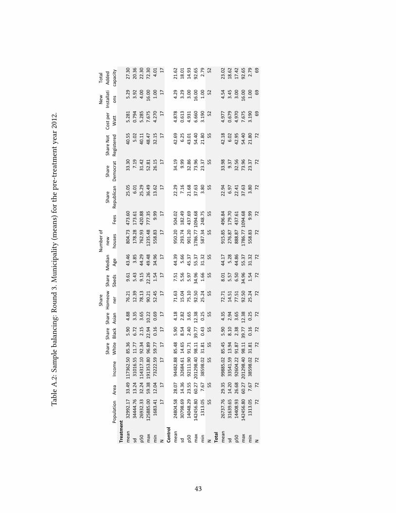
Table

A.2

:Sam

ple

balan

cin

g:

Ro

un

d3.

Mu

nicip

ality

(m

ean

s)

fo

rth

ep

re-treatm

en

ty

ear

2012.

Popu

latio

nArea

Income

Share

White

Share

Black

Share

Asian

Share

Homeo

wne

rShare

5bed

sMed

ian

Age

Num

bero

fne

w

houses

Fees

Share

Repu

blican

Share

Democrat

ShareNot

Registered

Costper

Watt

New

Installati

ons

Total

Adde

dcapacity

Treatm

ent

mean

32992.17

33.49

117362.50

85.36

5.90

4.88

76.21

9.61

43.46

804.73

473.60

25.05

33.30

40.55

5.281

5.29

27.30

sd34444.76

13.24

31016.55

11.77

6.72

3.35

12.39

5.43

3.85

178.28

173.61

6.01

7.19

5.02

0.794

3.92

20.36

p50

26932.33

32.24

114317.10

92.34

2.15

3.65

78.13

9.15

44.29

762.93

420.88

25.29

31.42

40.11

5.285

4.00

22.30

max

125885.00

59.38

191353.80

96.89

22.94

10.22

90.21

22.26

49.48

1235.48

777.35

36.49

52.81

48.47

7.675

16.00

72.30

min

1683.41

12.04

73222.59

59.77

0.16

0.69

52.45

1.54

34.96

558.83

9.99

13.62

26.15

32.15

4.270

1.00

4.01

N17

1717

1717

1717

1717

1717

1717

1717

1717

Control

mean

24804.58

28.07

94482.88

85.48

5.90

4.18

71.63

7.51

44.39

950.20

504.02

22.29

34.19

42.69

4.878

4.29

21.62

sd30798.69

14.36

32684.61

14.65

8.54

2.82

15.04

5.56

5.66

293.74

182.49

7.16

9.99

6.25

0.613

3.29

18.01

p50

14048.29

23.55

92111.90

91.71

2.40

3.65

75.10

5.97

45.37

901.20

437.69

21.68

32.86

43.01

4.931

3.00

14.93

max

142456.80

60.27

201298.40

98.11

39.77

12.38

92.50

34.96

55.37

1786.771094.68

37.63

73.96

54.40

6.660

16.00

92.65

min

1313.05

7.67

38598.02

31.81

0.43

0.25

25.24

1.66

31.32

587.34

248.75

3.80

23.37

21.80

3.190

1.00

2.79

N55

5555

5555

5555

5555

5555

5555

5552

5252

Total

mean

26737.76

29.35

99885.02

85.45

5.90

4.35

72.71

8.01

44.17

915.85

496.84

22.94

33.98

42.18

4.977

4.54

23.02

sd31639.65

14.20

33541.59

13.94

8.10

2.94

14.51

5.57

5.28

276.87

179.70

6.97

9.37

6.02

0.679

3.45

18.62

p50

14408.93

26.68

92604.22

91.87

2.38

3.65

77.51

6.50

44.86

888.87

437.61

22.41

32.56

42.95

4.970

3.00

17.42

max

142456.80

60.27

201298.40

98.11

39.77

12.38

92.50

34.96

55.37

1786.771094.68

37.63

73.96

54.40

7.675

16.00

92.65

min

1313.05

7.67

38598.02

31.81

0.16

0.25

25.24

1.54

31.32

558.83

9.99

3.80

23.37

21.80

3.190

1.00

2.79

N72

7272

7272

7272

7272

7272

7272

7269

6969

43

Table

A.3

:Sam

ple

balan

cin

g:

Ro

un

d5.

Mu

nicip

ality

(m

ean

s)

fo

rth

ep

re-treatm

en

ty

ear

2013.

Popu

latio

nArea

Income

Share

White

Share

Black

Share

Asian

Share

Homeo

wne

rShare

5bed

sMed

ian

Age

Num

bero

fne

w

houses

Fees

Share

Repu

blican

Share

Democrat

ShareNot

Registered

Costper

Watt

New

Installati

ons

Total

Adde

dcapacity

Treatm

ent

mean

13239.07

30.97

93764.69

84.11

7.65

5.25

81.84

10.93

46.25

847.96

492.08

28.99

29.59

39.81

4.648

6.45

37.93

sd9308.06

14.15

28503.81

15.44

13.22

3.07

5.82

7.22

5.17

216.95

111.43

7.56

6.80

4.18

0.337

3.45

20.22

p50

10388.22

30.15

87689.51

86.25

3.56

3.31

82.94

9.16

44.80

836.93

472.00

29.66

27.52

39.80

4.695

6.00

32.72

max

32515.20

62.09

159172.40

95.98

46.44

10.06

94.09

26.54

58.99

1283.11

778.72

43.23

48.78

47.20

5.095

11.00

60.11

min

2586.59

7.93

48797.09

41.53

0.31

1.85

72.97

1.63

39.49

571.78

364.00

14.13

24.51

31.06

3.940

1.00

3.88

N11

1111

1111

1111

1111

1111

1111

1111

1111

Control

mean

12949.68

28.49

89486.90

89.25

3.42

4.73

73.18

8.96

46.46

1095.26

434.79

24.52

31.53

43.01

4.661

6.04

33.33

sd10183.06

15.06

32963.19

6.47

3.56

3.35

10.86

7.17

5.32

415.95

137.76

6.02

6.36

5.24

0.504

5.78

31.65

p50

10445.95

23.55

80791.41

90.90

2.65

4.18

75.65

7.67

46.52

1002.12

392.51

23.35

30.96

43.57

4.674

4.00

21.59

max

34523.67

60.27

180719.30

98.46

23.70

14.14

91.69

44.44

60.46

2174.59

773.04

38.40

51.82

53.64

6.247

32.00

171.99

min

1283.64

7.67

42867.96

59.95

0.60

0.27

32.48

1.63

32.50

621.22

224.00

13.09

22.00

33.25

3.510

1.00

3.80

N45

4545

4545

4545

4545

4545

4545

4545

4545

Total

mean

13006.53

28.97

90327.18

88.24

4.25

4.84

74.88

9.35

46.42

1046.68

446.04

25.40

31.15

42.38

4.658

6.13

34.23

sd9935.89

14.80

31936.18

9.00

6.69

3.27

10.61

7.16

5.24

395.98

134.04

6.53

6.43

5.18

0.473

5.38

29.65

p50

10417.09

26.68

82901.77

90.82

2.69

3.94

76.43

7.97

46.18

977.45

412.00

24.18

28.93

42.67

4.683

4.00

24.02

max

34523.67

62.09

180719.30

98.46

46.44

14.14

94.09

44.44

60.46

2174.59

778.72

43.23

51.82

53.64

6.247

32.00

171.99

min

1283.64

7.67

42867.96

41.53

0.31

0.27

32.48

1.63

32.50

571.78

224.00

13.09

22.00

31.06

3.510

1.00

3.80

N56

5656

5656

5656

5656

5656

5656

5656

5656

44

Figure A.1: Pre-treatment trends. Comparison of treatment and control towns

050

100

150

200

Cum

ulat

ive

inst

alla

tions

2011m7 2012m7 2013m7 2014m7 2015m7Date

Control: CT CEC Solarize ChoiceSolarize Classic

Cumulative Installations by Treatment: Solarize R3

(a) Cumulative installations, R3

050

100

150

200

Cum

ulat

ive in

stal

latio

ns

2013m1 2014m1 2015m1 2016m1Date

Control: CT CEC Solarize OnlineSolarize Classic

Cumulative Installations by Treatment: Solarize R5

(b) Cumulative installations, R3

24

68

Mea

n C

ost p

er W

att

2011m7 2012m7 2013m7 2014m7 2015m7Date

Control: CT CEC Solarize ChoiceSolarize Classic

PPA excludedCost for Solar by Treatment: Solarize R3

(c) Price of Solar, R3

23

45

67

Mea

n Co

st p

er W

att

2013m1 2014m1 2015m1 2016m1Date

Control: CT CEC Solarize OnlineSolarize Classic

PPA excludedCost for Solar by Treatment: Solarize R5

(d) Price of Solar, R5

Note: Vertical lines indicate the start and end-date of Solarize campaigns. While the campaign

timing was coordinated in R5, due to logistical reasons Choice started with a two month lag after

Classic in R3.

45

Figure A.2: Histogram of main dependent variables

0.2

.4.6

.8De

nsity

2 4 6 8 10 12Cost

Note: Distribution of the cost of solar for treatment and control towns in Round 3. The sample is limited toOctober 2011 to May 2015.

(a) Price of solar, sample R3

0.2

.4.6

.8D

ensi

ty

0 5 10 15Cost

Note: Distribution of the cost of solar for treatment and control towns in Round 5. The sample is limited toDecember 2012 to December 2015.

(b) Price of solar, sample R5

0.1

.2.3

.4.5

Den

sity

0 10 20 30 40Number of new installations

Note: Distribution of new solar installations. R3 Sample.

(c) Number of new installations, sample R3

0.2

.4.6

Den

sity

0 10 20 30Number of new installations

Note: Distribution of new solar installations. R5 Sample.

(d) Number of new installations, sample R5

46

Figure A.3: Mean price of solar, by focal installer

34

5M

ean

pric

e / W

att

Classic: F Classic: NF Choice: F Choice: NF NoSolarize campaign

Note: Mean solar prices in 5-month intervals. Bar 1 in each group refers to the 5-month period pre-Solarize.Bar 2 to the 5 months of the campaign. Bar 3 to the 5-month period afterwards. All type of residential solarsystems included. Control towns did not participate in Solarize campaigns (55 Clean Energy Communities).F: Focal (selected) installer, NF: Non-focal installer.

Focal vs. Non-focal installersPrice of Solar: Round 3

a) Round 3: Classic, Choice and Control

34

5M

ean

price

/ W

att

Classic: F Classic: NF Online: F Online: NF NoSolarize campaign

Note: Mean solar prices in 5-month intervals. Bar 1 in each group refers to the 5-month period pre-Solarize.Bar 2 to the 5 months of the campaign. Bar 3 to the 5-month period afterwards. All residential solar systemsincluded. Control towns did not participate in Solarize campaigns (45 Clean Energy Communities).F: Focal (selected) installer, NF: Non-focal installer.

Focal vs. Non-focal installersPrice of Solar: Round 5

b) Round 5: Classic, Online and Control

47

Figure A.4: Mean �nancing shares

0.2

.4.6

.81

Fina

ncin

g sh

ares

Classic Choice No1 2 3 1 2 3 1 2 3

Note: Mean solar prices in 5-month intervals. Bar 1 in each group refers to the 5-month period pre-Solarize.Bar 2 to the 5 months of the campaign. Bar 3 to the 5-month period afterwards. All type of residential solarsystems included. Control towns did not participate in Solarize campaigns (55 Clean Energy Communities).

Solarize vs. Non-Solarize municipalitiesType of Financing: Round 3

Lease LoanPPA Purchasen/a

a) Round 3: Classic, Choice and Control

0.2

.4.6

.81

Fina

ncin

g sh

ares

Classic Online No1 2 3 1 2 3 1 2 3

Note: Mean solar prices in 5-month intervals. Bar 1 in each group refers to the 5-month period pre-Solarize.Bar 2 to the 5 months of the campaign. Bar 3 to the 5-month period afterwards. All type of residential solarsystems included. Control towns did not participate in Solarize campaigns (45 Clean Energy Communities).

Solarize vs. Non-Solarize municipalitiesType of Financing: Round 5

Lease LoanPPA Purchasen/a

b) Round 5: Classic, Online and Control

48

Figure A.5: System size in Solarize municipalities

0.0

5.1

.15

.2.2

5Ke

rnel

den

sity

0 5 10 15 20System size [kwac]

Pre-Solarize SolarizePost-Solarize

5-month pre/during/post campaignR3 Classic: Systemsize

0.0

5.1

.15

.2.2

5Ke

rnel

den

sity

0 5 10 15 20System size [kwac]

Pre-Solarize SolarizePost-Solarize

5-month pre/during/post campaignR3 Choice: Systemsize

a) Round 3: System size in 5 month intervals relative to Solarize.

0.0

5.1

.15

.2Ke

rnel

den

sity

0 5 10 15 20System size [kwac]

Pre-Solarize SolarizePost-Solarize

5-month pre/during/post campaignR5 Classic: Systemsize

0.0

5.1

.15

.2.2

5Ke

rnel

den

sity

0 5 10 15 20System size [kwac]

Pre-Solarize SolarizePost-Solarize

5-month pre/during/post campaignR5 Online: Systemsize

b) Round 5: System size in 5 month intervals relative to Solarize.

49

Figure A.6: Consumer survey: most important motivation to install solar

27.5%

34.9%

20.8%

10.1%

6.7%

Lower my monthly utility bill Concern for the environmentStabilize energy cost over time A short payback periodOther

Adopters, Solarize: R3Classic, N = 149

Single most important reason to install solar

(a) R3 Classic

44.6%

20.7%

28.3%

5.4%1.1%

Lower my monthly utility bill Concern for the environmentStabilize energy cost over time A short payback periodOther

Adopters, Solarize: Choice, N = 92

Single most important reason to install solar

(b) R3 Choice

36.3%

22.5%

17.6%

7.8%

10.8%2.9%2.0%

Lower my monthly utility bill Concern for the environmentStabilize energy cost over time Town sponsored programDiccount pricing (Solarize) A short payback periodOther

Adopters, Solarize: R5Classic, N = 102

Single most important reason to install solar

(c) R5 Classic

20.5%

29.5%22.7%

9.1%

15.9%2.3%

Lower my monthly utility bill Concern for the environmentStabilize energy cost over time Town sponsored programDiccount pricing (Solarize) A short payback period

Adopters, Solarize: Online, N = 44

Single most important reason to install solar

(d) R5 Online

Table A.4: Robustness R3: Wild Bootstrap

Coef p-value 95% CI

SolarizeR3Classic –0.286∗

0.074 [-0.543, -0.016]

SolarizeR3Choice –0.489∗∗∗

0.002 [-0.657, -0.328]

PostR3Classic 0.124 0.306 [-0.112, 0.352]

PostR3Choice –0.158 0.166 [-0.362, 0.039]

Observations 3976

R2

0.308

Clusters 72

50

Table A.5: Robustness R5: Wild Bootstrap

Coef p-value 95% CI

SolarizeR5Classic 0.146 0.168 [-0.025, 0.319]

SolarizeR5Online 0.004 0.977 [-0.135, 0.149]

PostR5Classic 0.004 1.000 [-0.125, 0.143]

PostR5Online –0.177 0.150 [-0.336, -0.030]

Observations 4401

R2

0.405

Clusters 56

Note: Regression follows main regression model (1), controlling for month and municipality �xed e�ects as well as

controls for system size, system mounting, and type of system �nancing. Standard errors obtained through wild

cluster bootstrap as developed in Cameron, Gelbach, and Miller (2008) with 1000 simulations.

Table A.6: R3 (price): sample selection

(1) (2)

SolarizeR3Classic –0.082 –0.283∗∗∗

(0.211) (0.096)

SolarizeR3Choice –0.708∗∗∗

–0.531∗∗∗

(0.198) (0.126)

PostR3Classic 0.135 0.146

(0.253) (0.106)

PostR3Choice –0.304∗∗

–0.158

(0.150) (0.132)

Observations 1185 3853

R2

0.295 0.303

Month FE Y Y

Municipality FE Y Y

51

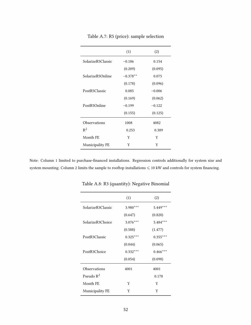
Table A.7: R5 (price): sample selection

(1) (2)

SolarizeR5Classic –0.186 0.154

(0.209) (0.095)

SolarizeR5Online –0.378∗∗

0.075

(0.178) (0.096)

PostR5Classic 0.085 –0.006

(0.169) (0.062)

PostR5Online –0.199 –0.122

(0.155) (0.125)

Observations 1008 4082

R2

0.253 0.389

Month FE Y Y

Municipality FE Y Y

Note: Column 1 limited to purchase-�nanced installations. Regression controls additionally for system size and

system mounting. Column 2 limits the sample to rooftop installations 6 10 kW and controls for system �nancing.

Table A.8: R3 (quantity): Negative Binomial

(1) (2)

SolarizeR3Classic 3.980∗∗∗

5.449∗∗∗

(0.647) (0.820)

SolarizeR3Choice 3.076∗∗∗

5.484∗∗∗

(0.588) (1.477)

PostR3Classic 0.325∗∗∗

0.355∗∗∗

(0.044) (0.065)

PostR3Choice 0.332∗∗∗

0.466∗∗∗

(0.054) (0.098)

Observations 4001 4001

Pseudo R2

0.178

Month FE Y Y

Municipality FE Y Y

52

Table A.9: R5 (quantity): Negative Binomial

(1) (2)

SolarizeR5Classic 2.833∗∗∗

3.112∗∗∗

(0.350) (0.405)

SolarizeR5Online 2.346∗∗∗

2.338∗∗∗

(0.396) (0.352)

PostR5Classic 0.979 1.078

(0.117) (0.299)

PostR5Online 0.954 0.939

(0.149) (0.120)

Observations 3129 3129

Pseudo R2

0.250

Month FE Y Y

Municipality FE Y Y

Note: Negative binomial estimation of model (2). The coe�cients can be interpreted as incidence-rate-ratios (IRR). Column 1 estimates the model with XTNBREG and reports standard

errors according to the observed variance-covariance matrix, while Column 2 uses the standard NBREG command with dummy variables to account for municipality �xed e�ects and reports

municipality-clustered standard errors.

53