Long and short-range air navigation on spherical Earth

International Journal of Aviation, International Journal of Aviation,

Aeronautics, and Aerospace Aeronautics, and Aerospace

Volume 4 Issue 1 Article 2

1-1-2017

Long and short-range air navigation on spherical Earth Long and short-range air navigation on spherical Earth

Nihad E. Daidzic AAR Aerospace Consulting, LLC, [email protected]

Follow this and additional works at: https://commons.erau.edu/ijaaa

Part of the Aviation Commons, Geometry and Topology Commons, Navigation, Guidance, Control and

Dynamics Commons, Numerical Analysis and Computation Commons, and the Programming Languages

and Compilers Commons

Scholarly Commons Citation Scholarly Commons Citation Daidzic, N. E. (2017). Long and short-range air navigation on spherical Earth. International Journal of Aviation, Aeronautics, and Aerospace, 4(1). https://doi.org/10.15394/ijaaa.2017.1160

This Article is brought to you for free and open access by the Journals at Scholarly Commons. It has been accepted for inclusion in International Journal of Aviation, Aeronautics, and Aerospace by an authorized administrator of Scholarly Commons. For more information, please contact [email protected].

http://commons.erau.edu/

http://commons.erau.edu/

https://commons.erau.edu/ijaaa

https://commons.erau.edu/ijaaa

https://commons.erau.edu/ijaaa/vol4

https://commons.erau.edu/ijaaa/vol4/iss1

https://commons.erau.edu/ijaaa/vol4/iss1/2

https://commons.erau.edu/ijaaa?utm_source=commons.erau.edu%2Fijaaa%2Fvol4%2Fiss1%2F2&utm_medium=PDF&utm_campaign=PDFCoverPages

http://network.bepress.com/hgg/discipline/1297?utm_source=commons.erau.edu%2Fijaaa%2Fvol4%2Fiss1%2F2&utm_medium=PDF&utm_campaign=PDFCoverPages







https://doi.org/10.15394/ijaaa.2017.1160

mailto:[email protected]

As the long-range and ultra-long range non-stop commercial flights slowly

turn into reality, the accurate characterization and optimization of flight

trajectories becomes even more essential. An airplane flying non-stop between

two antipodal points on spherical Earth along the Great Circle (GC) route is

covering distance of about 10,800 NM (20,000 km) over-the-ground. Taking into

consideration winds (Daidzic, 2014; Daidzic; 2016a) and the flight level (FL), the

required air range may exceed 12,500 NM for antipodal ultra-long flights. No

civilian or military airplane today (without inflight refueling capability) is capable

of such ranges. About 40-60% increase in air range performance will be required

from the future airplanes to achieve truly global range (GR). There is no need to

elaborate on the economic aspects of finding the shortest trajectories between two

points on Earth. However, many other factors may cause perturbations of such

trajectories when considering the minimum-cost, minimum-fuel, or any other

goal-function in complex optimizations.

The Earth is not a perfect sphere and due to rotational and gravitational effects

the shape is more of an oblate spheroid. Actually, Earth’s shape is even more

complicated and more appropriately treated in terms of tesseral surface harmonics

(Tikhonov and Samarskii, 1990). Earth’s Polar radius is about 21 km shorter than

the Equatorial. Several Earth’s shape approximations are used:

Idealized spherical Earth of equivalent volume (implicitly used in

International Standard Atmosphere or ISA definition).

Reference mathematical ellipsoid of revolution (WGS-84, IERS/ITRS).

Smooth and oblate.

Geoid or particular equipotential surface that approximates mean sea-level

(MSL). Irregular and locally smooth. Physically the most important measure

of Earth’s shape. An example of Geoid in use is WGS-84 (revision 2004)

EGM96 Geoid.

Actual or physical Earth surface with all terrain details. This is fractal

dimension, scale dependent and mathematically intractable.

Using spherical Earth approximation is sufficient for the majority of long-

range air navigation problems. Due to economy of flight, we are particularly

interested in the shortest distances between two arbitrary points on Earth.

Differential geometry classifies such lines on smooth surfaces as geodesic lines.

On the spherical Earth model a geodesic is a Great Circle (GC) or Orthodrome

segment. GCs distances are not necessarily always shortest with respect to time as

atmospheric wind plays significant role in distance-time optimization problems.

The optimization of flight trajectories taking into account atmospheric factors,

extended operations (ETOPS) procedures (De Florio, 2016; FAA, 2008), airspace

1

Daidzic: Air navigation on spherical Earth

Published by Scholarly Commons, 2017

restriction, etc., is a difficult task. Finding geodesics on smooth ellipsoidal Earth

has been solved. However, finding geodesic between two arbitrary points on the

actual Earth surface considering all the vertical terrain features is practically

impossible.

Although, it has been with us for many years, the theory of GC and

rhumb-line navigation has not been presented clearly and comprehensively for air

navigation practitioners, operators, and students. One of the stated purposes of

this article is to review and summarize differential geometry and calculus of

variation theories as applied to spheres. That will relive readers from searching

and consulting multiple sources using different and often confusing terminology.

We are only considering spherical Earth approximation and present theory

of GC (Orthodrome geodesic) and rhumb-line (Loxodrome) navigation. For short

distances over certain terrestrial regions we also provide some simplified

approximate formulas and define their limits of use. Several ultra-long-range

navigational problems utilizing existing major international airports are fully

solved using Orthodromes and Loxodromes. Graphic representation utilizing

Mercator (cylindrical) and azimuthal (planar) projections is presented. The

longest commercial non-stop flights today are reaching 8,000 NM (Daidzic,

2014). Increase in air range of, at least, 40% is required to achieve full GR

connecting any two airports on the Earth (Daidzic, 2014). Practically, due to

airspace restrictions, ETOPS procedures, and other considerations, the range of

existing long-range subsonic airplanes may need to increase by at least 50%.

The main purpose of this article is to give complete and comprehensive

consideration of short and long (geodesic) lines on spherical Earth for the purpose

of air navigation. While clearly professional navigation planning software is

available to major airlines/operators and ATC system it is mostly used as a black-

box. The objective is also to remove mysteries behind the long-range navigational

calculations and provide working equations. Spherical approximation is

satisfactory for overwhelming number of long-range air navigation problems. In

particular, Orthodromes and Loxodromes are typically considered the two most

important curves for air navigation. For that purpose we coded working equations

into several software platforms (Basic, Fortran, IDL, and Matlab). The main goal

of this article was to provide the fundamental theory and understanding, while the

computations can be executed in any high-level programming language.

Detailed mathematical derivations are presented in several appendices as

to relive a reader interested only in the final results from the heavy mathematical

interpretations involving differential geometry, variational calculus, topology and

2

International Journal of Aviation, Aeronautics, and Aerospace, Vol. 4 [2017], Iss. 1, Art. 2

https://commons.erau.edu/ijaaa/vol4/iss1/2DOI: https://doi.org/10.15394/ijaaa.2017.1160

other mathematical fields. Indeed, a knowledge of differential geometry, plane

and space vectors and vector calculus, and calculus of variation (variational

calculus) is required for in-depth understanding of the subject matters. The most

important geometric and topological properties of spheres have been reviewed

and working equations provided.

An added benefit of presented long-range navigation solutions is relatively

easy implementation of the actual Point-of-Equal-Time (PET), Point-of-No-

Return (PNR) and ETOPS limitations for given wind conditions (Daidzic, 2016a)

and one-engine-inoperative (OEI) cruising speeds (Daidzic, 2016b). In a future

contribution, and for the academic completeness an ellipsoidal Earth model will

be introduced with the Great Ellipse (GE) substituting Great Circle (GC). True

geodesic computations are complicated even for a smooth ellipsoid of revolution

requiring iterative solvers. Generally, GC calculations on spherical Earth are

sufficient for reliable air navigation flight planning purposes, considering all other

uncertainties involved and mandatory fuel reserves.

Air navigation should be a mandatory course in every professional pilot

curriculum and especially so in aviation university education. Unfortunately, it

often is not, which results in operational safety degradations. Too much and/or

uneducated reliance on sophisticated electronic navigation technology did and

certainly will continue to cause aviation accidents and incidents.

Literature review

A historic account of differential geometry and basic parts used in this

work have been consulted from the well-known mathematical classics, such as,

Aleksandrov et al. (1999), Goetz (1970), Kreyszig (1964), Lipshutz (1968), Struik

(1988), and Wrede (1972). Also more modern books on differential geometry,

such as, Oprea (2007) have been consulted. Basic planar and spherical

trigonometry theory with calculus applications has been consulted from the

books/handbooks by Ayres and Mendelson (2009), Bronstein and Semendjajew

(1989), Danby (1962), Dwight (1961), Nielsen and Vanlonkhuyzen (1954), Olza

et al. (1974), Spiegel and Liu (1999), and Todhunter (1886). The basic

introduction and theory of solid analytic geometry including various lines, planes

and curved surfaces was consulted using Hall (1968). A decent short history of

mathematical development including the planar and spherical trigonometry is

given in Struik (1987). Some special functions, elliptic integrals, and advanced

mathematical methods used in navigation, orbital, and celestial calculations is

given in classic sources by Abramowitz and Stegun (1984), Byrd and Friedman

(1954), Jahnke and Emde (1945), Tikhonov and Samarskii (1990), and Weber and

3



Arfken (2004). The general theory of calculus of variations and its applications in

analytical mechanics and geodesics on the sphere are given in, for example, Dym

and Shames (2013), Fox (1987), Greenwood (1987), Lanzos (1986), Lass (2009),

Smith (1998), Widder (1989), etc. An introduction into geodesy and geodetic

computations was consulted from the well-known classics such as Bomford

(1983), Torge (2001), and Vaníček and Krakiwsky (1986).

Basic principles of marine and air navigation and navigational

instrumentation are given in books by Bowditch’s bicentennial edition (2002),

Bradley (1942), De Remer and McLean (1998), Jeppesen (2007), Tooley and

Wyatt (2007), Underdown and Palmer (2001), and Wolper (2001). However, none

of these sources except maybe to an extent Wolper go into any deeper air

navigation mathematical theory and calculation procedures. Sinnott (1984)

proposed the use of the, so called, haversine formula for the GC navigation

problems on spherical Earth due to problems with numerical accuracy using the

classic cosine-formula for small central angles. Williams (2011) provides many

useful aviation formulas, but the equations are written as pseudo-language

mathematical expressions, difficult to read, and no background information is

provided. Phillips (2004) provides algorithms for GC and rhumb-line navigation,

but without derivations. Tewari (2007) presents GC and long-range airplane flight

computations and demonstrates how in the absence of wind with no yawing and

rolling motion, the airplane will actually follow a GC route. Recently, Weintrit

and Kopacz (2011) presented a novel approach to Loxodrome, Orthodrome, and

general geodesic problems in Electronic Chart Display and Information

System (ECDIS) used for nautical navigation.

Basic GC navigation theory also finds many applications is celestial

navigation, orbital mechanics, and astronomy and we used sources such as, Bate

et al. (1971) and Fitzpatrick (2012) for some useful information. Geodetic theory

and computations with geometric geodesy and geodetic datums on reference

terrestrial ellipsoid with some historical accounts has been provided in reports by

Jekeli (2012), Krakiwsky and Thomson (1974), Rapp (1991), and Rapp (1993).

Many geodetic computations also find applications in geophysics and we mention

some better known sources such as Lowrie (2007) that deal with various aspects

of geodetic geometry, definitions, and computations.

A good review of rhumb-line calculations on a sphere is given by

Alexander (2004) and for terrestrial ellipsoid by Williams (1950). Kos et al

(1999) derived and solved differential equation of Loxodrome on spherical Earth

using difference of co-latitudes to find its length. GE theory with geodesic and

rhumb-line calculations on spheroidal (ellipsoidal) Earth were given by Bennett

4



(1996), Bowring (1984), Sjöberg (2012), Tseng and Lee (2010), and Williams

(1996). A true numerical geodesic computations for direct and inverse geodesic

problems on ellipsoid of revolution (terrestrial spheroid) is given in a contribution

by Vincenty (1975). Consideration of elliptic integrals used in geodesic problems

was recently addressed by Rollins (2010). More recently Karney (2013) presented

a comprehensive account of algorithms for geodesics.

Motion of aircraft in an inertial frame of reference and non-inertial

topocentric frames was consider by Miele (2016). McIntyre (2000) provides in

depth considerations of motion on a rotating sphere. Fitzpatrick (2012) gives good

account of inertial and non-inertial frames of references on Earth. Discussion of

airplane trajectories and consideration of apparent forces in various non-inertial

frames of references during GC flights will be addressed in a future contribution.

Great Circle and Rhumb-line Navigation on Spherical Earth

Most often the inverse geodetic problem will be solved where the geodetic

(geographic) spherical coordinates of departure and arrival (destination) airports

are given. Sufficiently complete theory on fundamental geometric and topological

properties of spherical Earth is given in Appendix A. Derivation of geodesic lines

on spherical Earth, i.e., Orthodromes (GC arcs) is presented in Appendix B. The

GC arcs lie in an osculating plane that contains Earth’s center. A proof that GC

arcs are indeed shortest distances on spherical Earth is presented. Long distance

GC navigation on spherical Earth is discussed in Appendix C. The working

equations for calculating no-wind true courses (TC) and the vertex properties are

derived. GC and rhumb-line routes are plotted in cylindrical conformal Mercator

and/or polar Orthographic projections. Short-distance GC formulas were derived

in Appendix D. Additionally, stereographic, gnomonic and orthographic polar

(azimuthal) projections have been introduced. Theory of rhumb-line navigation on

spherical Earth is presented in Appendix E.

The traditional geographic latitude/longitude coordinates are first

converted into truncated angular degree form by using (N+, S-, E+, W-):

DDDDDDD.DDD,

SSSS.SSMMDDD

600360SS.SSSSMMDDD (1)

Geographic coordinates with an accuracy of one angular second (2.78x10-4

degree), provides an accuracy of about 100 ft (30 m). A hundredth of an angular

second delivers navigational uncertainty of about 1 ft (0.3 m). Eight significant

digits representation is thus sufficiently accurate for air-navigation applications.

5



Typically, aircraft fly at constant pressure altitudes, which at high altitudes

is referenced to a standard pressure datum (29.92 inch Hg or 1013.25 hPa). If

Earth’s oblateness is neglected and spatial changes of atmospheric pressure it can

be said that airplanes fly in concentric circles around Earth’s center. In that case

any GC will have arc-length of about 21,600 NM (or about 40,000 km or 25,000

SM). Future ultra-long range airplane should be able to fly non-stop half of any

GC to a point which is exactly opposite on the Earth surface (antipodal or

conjugate point) to achieve global range (Daidzic, 2014). Between two antipodal

points there are infinitely many GCs all of which have equal length assuming

spherical earth. The actual terrain elevation is irrelevant in high-altitude cruise

flight. Orthometric or Mean Seal Level (MSL) altitude is given in reference to

local Geoid height. Terrain elevation can be given in respect to vertical datum

contained in WGS 84 spheroid (GPS reference ellipsoid) and when corrected for

local Geoid height yields orthometric height. More accurate trajectory

calculations should also account for orthometric altitude changes due to variable

air pressure, but such considerations may not be significant for majority of flights.

Distance errors due to the actual shape of the Earth are less than 0.5% and often

within 0.3% and thus practically insignificant for most cases.

Utilizing the spherical Law of Cosines (Appendix C) and the average

Earth radius ER (=6,371,000 m) plus the average cruising altitude h , the actual

GC arc distance between two surface points 111 ,P and 222 ,P becomes:

2121

1

21 1 sinsincoscoscoscosRhRO EE

(2)

An alternative GC-arc distance formula using the trigonometric haversine

function (Appendix C) yields:

haverscoscoshavers

haverscoscoshaverstanRhR

sincoscossinsinRhRO

EE

EE

21

211

2

21

21

21

112

2212

(3)

Adding the average cruising altitude, or the maximum planned cruising

altitude, does not affect GC distance very much (10-20 NM), but is a conservative

estimate reducing uncertainties. All courses, vertex properties, and GC and

rhumb-line waypoints were calculated using expressions derived in appendices.

The geographical coordinates are given as latitudes ϕ (N+, S-) and longitudes λ

(W-, E+) for desired airport pairs on spherical Earth. The geodetic coordinates of

6



some major international airports used in program testing and route calculations

are given in Table 1.

Table 1

Airports used in long- and ultra-long range route computations and testing

ICAO IATA City Latitude (N+/S-)

DD MM SS.SSSS

Longitude (E+/W-)

DDD MM SS.SSSS

ZBAA PEK Beijing,

China

N 40 04 00.0000 E 116 36 00.0000

+40.08000000 +116.58444444

ZSPD PVD Shanghai,

China

N 31 09 00.0000 E 121 48 00.0000

+31.1500000 +121.8000000

SAEZ EZE Buenos Aires,

Argentina

S 34 49 20.0000 W 058 32 09.0000

-34.822222222 -58.53583333

RJAA NRT Tokyo-Narita,

Japan

N 35 45 55.0000 E 140 23 08.0000

+35.765278 +140.385556

SBGL GIG Rio de Janerio,

Brazil

S 22 48 32.0000 W 043 14 37.0000

-22.808902 -43.243646

KSEA SEA Seattle, WA,

United States

N 47 27 00.0000 W 122 18 42.0000

+47.449889 -122.311777

EGGL LHR London, England,

UK

N 51 28 39.0000 W 000 27 41.0000

+51.477500 -0.461388

YSSY SYD Sydney, Australia S 33 56 46.0000 E 151 10 38.0000

-33.946110 +151.177222

FAOR JNB Johannesburg,

South Africa

S 26 08 01.0000 E 028 14 32.0000

-26.133693 28.242317

MMMX MEX México City,

México

N 19 26 11.0000 W 099 04 20.0000

+19.436303 -99.072096

WMKK KUL Kuala Lumpur,

Malaysia

N 02 44 44.0000 E 101 42 36.0000

+2.745578 +101.709917

UUEE SVO Moscow, Russian

Federation

N 55 58 21.0000 E 037 24 47.0000

+55.972500 +37.413056

VCBI CMB Colombo, Sri

Lanka

N 07 10 51.0000 E 079 53 03.0000

+7.180756 +79.884117

SEQM UIO Quito, Pichincha,

Ecuador

S 00 06 48.0000 W 078 21 31.0000

-0.113332 -78.358610

LQSA SJJ Sarajevo, Bosnia

and Herzegovina

N 43 49 29.0000 E 018 19 53.0000

+43.82472222 +18.33138889

KMSP MSP Minneapolis-STP,

MN, United States

N 44 52 55.0000 W 093 13 18.0000

+44.88194444 -93.22166667

7



https://tools.wmflabs.org/geohack/geohack.php?pagename=Minneapolis%E2%80%93Saint_Paul_International_Airport&params=44_52_55_N_093_13_18_W_type:airport_region:US-MN

https://tools.wmflabs.org/geohack/geohack.php?pagename=Minneapolis%E2%80%93Saint_Paul_International_Airport&params=44_52_55_N_093_13_18_W_type:airport_region:US-MN

Rhumb-line or Loxodrome-arc distance of constant course angle α on

spherical Earth is calculated as (Appendix E):

secRhR

cosRhRL EEEE

12

1221 11 (4)

Special care has to be taken to convert spherical angles into Earth-based

headings 0-360 degrees. Attention also was warranted when crossing the prime

and its anti-meridian or practically the International Date Line (IDL). The cyclic

non-unique nature of trigonometric functions creates many problems when

performing calculations as illustrated in Figures 1 and 2. The main navigation

program originally developed in the True Basic v.5.5 contains subroutines that

inspect each airport location and then calculate route waypoints and courses.

Figure 1. Change of latitude on spherical Earth model. Not to scale.

Navigational calculations were performed on a multi-core 64-bit floating-

point CPU to minimize rounding errors. True Basic v.5.5 and v.6 (64-bit), 32-bit

optimizing-compiler Lahey Fortran 90/95 (Incline Village, NV), 64-bit optimizing

Absoft Fortran 90/95 (Troy, MI) with many 2003/2008 extensions, and Matlab

R2015a (ver. 8.5, Mathworks, Natick, MA) codes were developed with the

graphical capabilities showing GC and Rhumb-line routes on Cylindrical

Mercator and Polar Orthographic projections. Summary of some tested long-range

route computations using loxodromic and orthodromic navigation is given in

Table 2. Most GC (no rhumb-line) graphical results were generated using the

Great Circle Mapper©, copyright Karl L. Swartz (www.gcmap.com). Our

8



http://www.gcmap.com/

graphical capabilities are currently modest, but powerful visual representations

using IDL (Interactive Data Language) mapping capabilities will be available

soon. Several ultra-long routes between some major International airports were

used to test and demonstrate the capability and the accuracy of our NAV solvers.

Moreover, the intention was to highlight the difficulties and the curiosities when

navigating on Earth. Our AARNAVTM navigation programs used spherical-Earth

approximation, while the GC Mapper© calculator uses geodesic calculations on

oblate Earth. We also used the marine navigation www.Onboardintelligence.com

calculator to independently test and verify GC and rhumb-line results.

Figure 2. Change of longitude on spherical Earth model. Not to scale.

Results and discussion

Let us first consider a short flight from ZBAA to ZSPD. Interestingly,

Beijing (ZBAA) and Shanghai (ZSPD) are only 594.38 NM orthodromic-distance

apart (at FL360) with the Shanghai being S-SE of Beijing (numerical results are

summarized in Table 2). The ZBAA orthodrome departure course of 153.084o and

the ZSPD arrival course is 156.127o (see Table 2). The loxodrome constant course

and distance are 154.689o and 594.45 NM respectively (only about 0.07 NM or

about 426 ft longer). The vertex (Lat/Long) of the ZBAA to ZSPD GC-route is

located outside of the arc segment at N69.73/E044.69.

The first long-range route we discuss is the route between the SAEZ and

ZBAA (Daidzic, 2014). The Orthodrome distance flying at 36,000 ft delivers

distance of 10,433.26 NM. The initial outbound heading (from SAEZ) is 34.92o

9



http://www.onboardintelligence.com/

and the final inbound heading (at ZBAA) is 142.11o with the northerly vertex of

N61.97o at E053.20o longitude. The total change in heading is about 107o. The

illustration of the GC route is shown in Figure 3. GC Mapper© oblate-Earth

(WGS-84) calculator returned the geodesic distance within 2.3 NM of our

orthodrome computations. The geodesic route overflies eastern parts of Brazil,

crosses Atlantic ocean northbound and tracks parallel to the coast of western

Africa, skimming N-W Europe and N-W portions of Russia and then after

reaching vertex it “descends” over Mongolia to Beijing on SE headings.

Table 2

Long-distance Loxodromic (L1-2) and Orthodromic (O1-2) routes at FL 360

Route L1-2 [NM] L O1-2 [NM] 1 2 Vertex

Lat.

ZBAA-ZSPD 594.45 154.69 594.38 153.08 156.13 N69.73

SAEZ-ZBAA 10,730.47 65.18 10,433.26 34.92 142.11 N61.97

SAEZ-ZSPD 10,930.39 291.28 10,604.11 184.38 355.80 S86.41

SBGL-RJAA 10,656.37 289.31 10,023.92 347.13 194.66 N78.15

SEQM-WMKK 10,819.16 270.91 10,667.53 358.51 181.49 N88.51

KSEA-FAOR 9,329.08 118.32 8,934.82 57.79 140.41 N55.10

EGGL-YSSY 9,578.70 122.44 9,206.03 60.46 139.22 N57.19

MMMX-WMKK 9,414.94 263.88 9,012.50 315.12 221.77 N48.29

MMMX-VCBI 10,477.80 94.03 9,223.85 2.31 177.80 N87.82

LQSA-KMSP 4,797.61 270.76 4,359.97 316.29 224.72 N60.10

The rhumb-line distance SAEZ-ZBAA is 10,730.47 NM (Loxodrome is

about 297.22 NM or 2.85% longer than Orthodrome) on a constant heading of

about 65.180 and includes about 3,500 NM flight over the dangerous southern

Atlantic Ocean. Rudimentary graphs were superimposed on a publically-available

conformal Mercator projection image of the world as shown in Figure 4

(Latitudes are unevenly spaced as ±15, ±30, ±45, ±60, and ±75 degrees). The GC

(red solid line) and rhumb-line (blue solid line) routes are clearly discernable. The

apparently shorter rhumb-line is quite deceptive due to stretching of the scale at

higher latitudes on conformal Mercator projection. The difference between the

GC route and the true Geodesic using GC Mapper is very small.

10



https://tools.wmflabs.org/geohack/geohack.php?pagename=Sarajevo_International_Airport&params=43_49_29_N_018_19_53_E_type:airport_region:BA-09

Figure 3. Great circle (geodesic) route SAEZ to ZBAA (EZE to PEK) on

conformal cylindrical Mercator chart. Courtesy of GC Mapper. Maps generated

by the Great Circle Mapper (www.gcmap.com) - copyright © Karl L. Swartz.

Figure 4. GC route SAEZ to ZBAA on conformal cylindrical Mercator chart.

11



The long-range route from SAEZ to ZSPD is illustrated in Figure 5 using

GC Mapper© and Mercator cylindrical projections. The same flight is partially

also shown in Figure 6 using Polar Orthographic projection. In the case of SAEZ-

ZSPD, the shortest (orthodrome) distance at FL360 is over Antarctica (SP) at

10,604.11 NM and a mere 200 NM short of antipodal distance.

Figure 5. Geodesic route SAEZ to ZSPD on conformal cylindrical Mercator

chart. Courtesy of GC Mapper. Maps generated by the Great Circle Mapper

(www.gcmap.com) - copyright © Karl L. Swartz.

The initial outbound heading from SAEZ is now almost straight south or

about 184o, while the final inbound heading to destination ZSPD is about 356o.

The vertex is very close to SP at -86.41o. The rhumb-line distance is 10,930.39

NM at the constant heading of 291.28o (see Table 2) and involves diagonal flight

over the entire Pacific Ocean. The GC Mapper returned the value of 10,580 NM

(over surface) with the departure heading of 183.9o. None of the two SAEZ-ZSPD

routes (GC or rhumb-line) are particularly friendly in terms of ETOPS procedures

as they involve long flights over Polar Regions and oceans. What is very

interesting is that while destinations ZBAA and ZSPD are very close to each

other, the routes from SAEZ could not be more different. One reaches high

northern latitudes, while the other goes almost straight over the South Pole (SP)

and straight across Antarctica.

If such a direct non-stop flight is ever planned it would be perhaps better

in terms of safety and following the ETOPS procedures to follow similar route as

in SAEZ-ZBAA route, i.e., fly over the South- and the North-America, passing

12



close to the North Pole (NP) and approach ZSPD on an almost straight south

course. Such longer route would probably add another 1 ½ hour of flight, but

there would be more options for deviations and alternates. Thus to have truly

global range an airplane will have to have practical ground range exceeding half

of the Earth circumference (e.g., 12,000 NM over ground) in which case the

required air range would likely exceed 13,000 NM.

Figure 6. SAEZ to ZSPD geodesic route on Polar Orthographic chart. Courtesy of

GC Mapper. Maps generated by the Great Circle Mapper (www.gcmap.com) -

copyright © Karl L. Swartz.

The next possible future ultra-long range flight specifically considered is

from Rio de Janerio (Brazil) SBGL (GIG) to Tokyo Narita in Japan RJAA (NRT).

The route is shown in Figure 7 on Mercator chart and in Figure 8 on Polar

orthographic chart using GC Mapper©. According to Table 2’s summary of

several ultra-long routes, we have the rhumb-line distance of 10,656 NM on a

straight W-NW course of 289.31o while the GC distance with average cruise

altitude of 36,000 ft delivers 10,023.92 NM. The differences between the GC and

rhumb-line is quite significant at about 632.45 NM. Our calculator returned

347.13o for outbound and 194.66o for inbound course. Our calculations estimated

vertex at +78.15o latitude (North). We also utilized Onboardintelligence.com

13



(Onboard Marine navigation software) calculator and obtained 10,001.52 NM for

Orthodrome (over surface) with the departure heading of 347.4o and the inbound

course into Narita of 194.4o. Its vertex calculations resulted in +78°24'.15 latitude

and -138°09'.22 longitude. Similar results were also obtained using the GC

Mapper©, which returned 10,004 NM and 347.5o geodesic over the reference

ellipsoidal surface (WGS-84).

Figure 7. GC (geodesic) route SBGL to RJAA (GIG to NRT) on conformal

cylindrical Mercator chart. Courtesy of GC Mapper. Maps generated by the Great

Circle Mapper (www.gcmap.com) - copyright © Karl L. Swartz.

The last route we specifically discuss is also the longest flight of all

identified here between the existing major airports. In Figures 9 and 10 the route

between Quito (Ecuador) and Kuala Lumpur (Malaysia) or SEQM to WMKK

(UIO to KUL) are shown respectively on the Polar Orthographic and the Mercator

charts. Both cities lie almost exactly on Equator and are very close to be

antipodal. Our navigation calculator returned the value of 10,667.53 NM for GC

distance flying average altitude of 36,000 ft with outbound initial heading of

358.510o and inbound destination heading into WMKK on 181.492o heading. The

vertex calculated is at Lat/Long +88.5099o/-169.850o and which is only about 90

NM from the NP. Detailed listing of the route is given in Appendix F.

The rhumb-line calculations returned the distance of 10,819.16 NM at a

constant heading of 270.91o. The GC Mapper returned the value of 10,644 NM

for the shortest (geodesic) distance over oblate Earth. However, that is surface

distance and if we add about 18 NM for additional air distance we arrive at 10,662

14



NM which is within 6 NM (0.052%) of our calculations. GC Mapper returned a

value of 358.8o for outbound course from departure point SEQM, which is within

18 angular minutes of our calculations. The Onboardintelligence.com calculator

returned the value of 10,644.04 NM for the Orthodrome and 10,812.68 at 270.9o

for the Loxodrome. The GC departure course calculated is 360o and destination

inbound course is 181.2o. Vertex is at N88°47'.3 and W168°21'.3. Due to actual

oblateness of the Earth, the shortest distance between two locations close to

Equator and on opposite meridians very likely will go over the NP or the SP.

Figure 8. Geodesic route SBGL to RJAA (GIG to NRT) on Polar Orthographic



A familiar example of long-range route within continental US is flight

from KJFK (New York) to KLAX (Los Angeles). Our calculations have been

verified against Phillips’ (2004). A GC route at FL360 is 2,148.87 NM long with

the outbound course of 273.858o and the KLAX inbound of 245.892o. The vertex

is reached shortly after departing KJFK westbound. The rhumb-line distance is

2,169.77 NM at constant 259.324o TC and just about 21 NM longer than the

Orthodrome. Many examples of long-range flights (see Table 2) do not show very

large difference between the GC and rhumb-line distances – often less than 5%

(except MMMX-VCBI). In fact, the difference is largest when flying between two

points of similar mid-latitudes. For example, KMSP (Table 1) and Urumchi

(Ürümqi) Diwopu International Airport in China, Xinjiang/Uyghur province

(ICAO: ZWWW, IATA: URC) with latitude +43.908o and longitude of +87.475o,

are practically located on a meridian and its anti-meridian (longitude change of

15



179.3o). Both are located around the 44th parallel (like Sarajevo/LQSA). In fact

the central angle (about 91.21o) of the two airports lies in an osculating plane

slicing almost exactly over the NP. The orthodrome-arc length on the surface of

the spherical Earth is 10,142.1 km (5,476.3 NM), while the Loxodrome will

almost follow 44th parallel. The Loxodrome is about 14,244.6 km (7,691.5 NM)

which is about 40.5% longer than the GC-arc. Rhumb-line flying will imply

following straight East or West TC while the Orthodrome departure from KMSP

is almost on a straight North TC. Flying at FL360 will add about 10 NM. Flight

LQSA to KMSP shows 9.1% difference between the GC and the rhumb-line.

Figure 9. Geodesic route SEQM to WMKK (UIO to KUL) on Polar Orthographic



It must be said that GC distance calculations are very robust as they

involve cosines which is an even function. On the other hand course calculations

are fragile and considerable effort was made to make spherical-angles

16



transformation into Earth’s coordinates accurate under all conditions. All test

routes evaluated at MSL showed excellent agreement with the available terrestrial

spheroid geodesic calculators. However, these publically-available calculators are

black-boxes with no insight to inner workings, plus they do not offer the ability to

include altitude corrections. Our GC and rhumb-line courses and angles

computations also showed excellent agreement with other calculators. Hence, we

gained confidence in our navigation programs which can calculate almost any

route on Earth with sufficiently high accuracy apart from the true antipodal

distances for which the problem becomes undetermined on the spherical Earth.

Figure 10. Geodesic route SEQM to WMKK (UIO to KUL) on conformal

cylindrical Mercator chart. Courtesy of GC Mapper. Maps generated by the Great

Circle Mapper (www.gcmap.com) - copyright © Karl L. Swartz.

A common misconception when considering GC-route flying is that

somehow since it is a curve on Mercator chart it should be approximated by

straight line (secant) segments. As a matter of fact as long as the weight vector

remains in the osculating plane no change of flight course is required for non-

rotating planet. In the absence of wind and GC trajectories, an aircraft only needs

to assume the correct initial heading and continue with no rolling and/or yawing

motion. GC arc is a geodesic with the projection on a tangential plane being a

straight line and thus shortest distance. The geodesic curvature is zero. The effect

of Coriolis force exists for rotating planet and will be discussed in a future

contribution. It is in fact the loxodromic route that requires yawing motion to

maintain constant heading on spherical Earth (see Figure C2). Loxodrome ends up

being an infinite logarithmic spiral of finite length that winds around the pole.

17



We are currently implementing IDL mapping capabilities using various

Earth projections. An older licensed RSI’s IDL v.5.6 (2002) is being currently

used. Generally, IDL (newest v.8.6 by Harris Geospatial) has very rich and

powerful mapping and plotting capabilities and can work as standalone program

or as a graphic interface to modern Fortran, Matlab, and Basic programs.

Calculations of segment PNR and PET for given aircraft model in arbitrary wind

conditions (Daidzic, 2016a) are easily implemented. Also all-engines-inoperative

gliding performance with arbitrary wind can be added for routes. Some of the

calculated routes from Table 2 can be easily verified manually using the basic

Orthodrome and Loxodrome distance formulas given in Equations (2-4). More

improvements and testing will be conducted in the future on our AARNAVTM air-

navigation calculators adding more graphic features and capabilities and

enhancing performance. GC and rhumb-line waypoints can be calculated or for

equidistant arc segments or for constant longitude increments (Appendix F).

Loxodrome, GE, and true geodesic calculations on reference WGS-84 ellipsoid

will be added to GC and loxodrome calculations on spherical Earth.

Short lines on spherical Earth

First we test polar short-distance calculators based on the planar

projections. As an example we took two points on Antarctica close to the SP -

point 1 has coordinates S80o 20’ 30.5000” and E100o 30’ 40.3456”, while point 2

has coordinates S85o 10’ 44.7575” and E150o 45’ 20.0000”. The exact GC

inverse-cosine and inverse haversine formulas both returned the value of

453.43222 NM (839.75647 km), while the Law-of-Cosine flat-Earth

approximation (Equation D2) returned the value of 453.1708446 NM. The

difference is less than 1,590 ft or about 484 m (0.058% error), which is excellent

accuracy for distance of about 840 km.

Several right-angle very short-distance calculations (Equation D4) and

comparison with the true GC formulas were also conducted. Mankato regional

airport (KMKT) has coordinates (N44o 13’ 22.0000” and W093o 55’ 09.5000”). A

close by Le Sueur (12Y) airport is almost straight true North (TN) with the

coordinates (N44o 26’ 27.1971” and W093o 54’ 57.0502”). Our GC calculators

using inverse-cosine and inverse haversine formulas (Equations 2 and 3) both

returned distance of 13.118826 NM, while the planar approximation (Equation

D4) returned the value of 13.09708846 NM, which is only about 132.16 ft (40.28

m) difference. In another example, for two points close to equator with the change

of latitude of 10 arc-minutes (about 10 NM) symmetric across the equator and the

difference of longitude of 10 arc-minutes, the exact formulas return equal distance

18



of 14.17603 NM (26.254 km), while the flat-Earth approximation returns the

value of 14.15167 NM, which is only 148.08 ft or less than 0.17% error.

On the other hand if we use KMKT as departure airport again and utilize

the flat-Earth approximation to calculate distance to a nearby Waseca airport

(KACQ), which is just about 9 arc-minutes to the south and 22 arc-minutes to the

East at about 44th parallel, we obtain “straight” distance of 23.753 NM. This is 5+

NM (actually 33,867 ft) longer than the exact inverse-cosine or haversine GC

formula delivering about 18.183 NM and thus unacceptably inaccurate. The short-

line distance formula given with Equation (D4) is acceptable only up to about 15

NM (28 km) in equatorial and lower mid-latitudes. Calculations were performed

utilizing 32 and 64-bit floating point arithmetic with MS Excel, True Basic v. 5.5

and v.6, Fortran 90/95/2003/2008, and Matlab R2015a (8.5) high-level computer-

language codes. We anticipate that a more user-friendly and thoroughly tested

program version will be offered in the future for free to all users in public domain.

Conclusions

Global range air navigation implies flying non-stop from any airport to

any other airport on Earth. That requires airplanes with the operational air range

of at least 12,500 NM. Air transportation economy requires shortest distance

flights which in the case of spherical Earth are Orthodrome arcs. Rhumb-line

navigation has no practical application in long-range flights but has been used as

comparison for historical reasons. Great Circle routes between many major

international airports have been calculated and waypoints presented for both GC

and rhumb-line routes. Many future global-range flights may be prohibited due to

polar crossings and/or long flights over open water with not many alternate

landing sites available. Additionally, we summarized short-lines navigation theory

with particular emphasis on Polar Regions and very short distances elsewhere on

the Earth. Working equations and algorithms have been coded into several high-

level programming languages. Considerable testing of programs have been

conducted and compared with the publically-available geodesic computations

over the surface of the terrestrial reference ellipsoid. Distance computations

usually were less than 0.3% in error, while the angles and courses were mostly

within few angular minutes. Accurate database of about 50 major international

airports from every corner of the world has been constructed and used in testing

and route validation. Further development will include computations of gliding

distances from any altitude under arbitrary winds depending on the type of aircraft

and the calculations of PET and PNR for every segment of the route and arbitrary

wind conditions. A user-friendly machine-independent program version for global

navigation with many flight planning features will be posted to public domain.

19



Author Bios

Dr. Nihad E. Daidzic is president of AAR Aerospace Consulting, L.L.C. He is also

a full professor of Aviation, adjunct professor of Mechanical Engineering, and

research graduate faculty at Minnesota State University. His Ph.D. is in fluid

mechanics and Sc.D. in mechanical engineering. He was formerly a staff scientist

at the National Center for Microgravity Research and the National Center for

Space Exploration and Research at NASA Glenn Research Center in Cleveland,

OH. He also held various faculty appointments at Vanderbilt University,

University of Kansas, and Kent State University. His current research interest is

in theoretical, experimental, and computational fluid dynamics, micro- and nano-

fluidics, aircraft stability, control, and performance, mechanics of flight, piloting

techniques, and aerospace propulsion. Dr. Daidzic is ATP and “Gold Seal”

CFII/MEI/CFIG with flight experience in airplanes, helicopters, and gliders.

20



References

Abramowitz, M., Stegun, I. A. (1984). Handbook of mathematical functions

(abridged edition). Frankfurt (am Main), Germany: Verlag Harri Deutsch.

Aleksandrov, A. D., Kolmogorov, A. N., & Lavrent’ev, M. A. (1999).

Mathematics: Its content, methods and meaning (3 volumes translation

from Russian). Mineola, NY: Dover.

Alexander, J. (2004). Loxodromes: A rhumb way to go, Mathematics Magazine,

77(5), 349-356. DOI: 10.2307/3219199

Ayres, F., Jr., & Mendelson,E. (2009). Calculus (5th ed.). New York, NY:

McGraw-Hill.

Bate, R.R., Mueller, D. D., & White J. E. (1971). Fundamentals of astrodynamics.

New York, NY: Dover.

Bennett, G. G. (1996). Practical rhumb line calculations on a spheroid. Journal of

Navigation, 49(2), 112-119. DOI: 10.1017/s0373463300013151

Bomford, G. (1983). Geodesy (reprinted 4th ed.). New York, NY: Oxford

University Press.

Bowditch, N. (2002). The American Practical Navigator (2002 bicentennial ed.).

Bethesda, MD: National Imagery and Mapping Agency (NIMA).

Bowring, B. R. (1984). The direct and inverse solutions for the great elliptic line

on the reference ellipsoid. Bulletin Géodésique 58(1), 101–108. DOI:

10.1007/BF02521760

Bradley, A. D. (1942). Mathematics of air and marine navigation with tables.

New York, NY: American Book Company.

Bronstein, I. N., & Semendjajew, K. A. (1989). Taschenbuch der Mathematik (24.

Auflage). Frankfurt/Main, Germany: Verlag Harri Deutsch.

Byrd, P. F., & Friedman, M. D. (1954). Handbook of elliptic integrals for

engineers and physicists. Berlin, Germany: Springer Verlag.

21



Daidzic, N. E. (2014). Achieving global range in future subsonic and supersonic

airplanes. International Journal of Aviation, Aeronautics, and Aerospace

(IJAAA), 1(4), 1-29. DOI: 10.15394/ijaaa.2014.1038

Daidzic, N. E. (2016a). General solution of the wind triangle problem and the

critical tailwind angle, The International Journal of Aviation Sciences

(IJAS), 1(1), 57-93.

Daidzic, N. E. (2016b). Estimation of performance airspeeds for high-bypass

turbofans equipped transport-category airplanes. Journal of Aviation

Technology and Engineering (JATE), 5(2), pp. 27-50. DOI: 10.7771/2159-

6670.1122

Danby, J. M. A. (1962). Fundamentals of celestial mechanics. New York, NY:

MacMillan.

De Florio, F. (2016). Airworthiness: An introduction to aircraft certification and

operations (3rd ed.). Oxford, UK: Butterworth-Heinemann.

De Remer, D., & McLean, D. W. (1998). Global navigation for pilots (2nd ed.).

Newcastle, WA: Aviation Supplies and Academics, Inc.

Dym, C. L., Shames, I. H. (2013). Solid mechanics: A variational approach

(Augmented edition). New York, NY: Springer. DOI: 10.1007/978-1-

4614-6034-3

Dwight, H. B. (1961). Tables of integrals and other mathematical data (4th ed.).

New York, NY: Macmillan.

Fitzpatrick, R. (2012). An introduction to celestial mechanics. Cambridge, UK:

Cambridge University Press.

Fox, C. (1987). An introduction to the calculus of variation. Mineola, NY: Dover.

Goetz, A. (1970). Introduction to differential geometry. Reading, MA: Addison-

Wesley.

Greenwood, D. T. (1987). Classical dynamics. New York, NY: Dover.

Hall, J. E. (1968). Analytic geometry. Belmont, CA: Brooks/Cole Publishing Co.

22



Jahnke, E., & Emde, F. (1945). Tables of functions: With formulae and curves.

New York, NY: Dover.

Jekeli, C. (2012). Geometric reference systems in geodesy. Columbus, OH: State

University.

Jeppesen. (2007). General navigation. (JAA ATPL Training, Edition 2, Atlantic

Flight Training, Ltd., Sanderson Training products), Neu-Isenburg,

Germany: Author.

Karney, C. F. F. (2013). Algorithms for geodesics. J. Geod., 87, pp. 43-55. DOI:

10.1007/s00190-012-0578-z

Kos, S., Vranić D., & Zec, D. (1999). Differential equation of a loxodrome on a

sphere. Journal of Navigation, 52(3), 418-420. DOI:

10.1017/s0373463399008395

Krakiwsky, E. J., & Thomson, D. B. (1974). Geodetic position computations.

Dept. of Geodesy and Geomatics Engineering, Lecture Notes (39),

Fredericton, N.B., Canada: University of New Brunswick.

Kreyszig, E. (1964). Differential geometry (revised ed.). Toronto, Canada;

University of Toronto Press.

Lanczos, C. (1986). The variational principles of mechanics (4th ed.). Mineola,

NY: Dover.

Lass, H. (2009). Elements of pure and applied mathematics. Mineola, NY: Dover.

Lipschutz, M. M. (1969). Differential geometry. New York, NY: McGraw-Hill.

Lowrie, W. (2007). Fundamentals of geophysics (2nd ed.). Cambridge, UK:

Cambridge University Press.

McIntyre, D. H. (2000). Using great circles to understand motion on rotating

sphere. Am. J. Phys., 68(12), 1097-1105, DOI: 10.1119/1.1286858

Miele, A. (2016). Flight mechanics: Theory of flight paths. Mineola, NY: Dover.

23



https://doi.org/10.1017/s0373463399008395

http://dx.doi.org/10.1119/1.1286858

Nielsen, K. L., & Vanlonkhuyzen, J. H. (1954). Plane and spherical

trigonometry. New York, NY: Barnes & Noble.

Olza, A., Taillard, F., Vautravers, E., & Diethelm, J. C. (1974). Tables

numériques et formulaires. Lausanne, Switzerland: Spes S.A.

Oprea, J. (2007). Differential geometry and its applications (2nd ed.).

Washington, DC: The Mathematical Association of America.

Phillips, W. F. (2004). Mechanics of flight. New York, NY: John Wiley & Sons.

Rapp, R. H. (1991). Geometric geodesy: Part I. Columbus, OH: State University.

Rapp, R. H. (1993). Geometric geodesy: Part II. Columbus, OH: State University.

Rollins, C. M. (2010). An integral for geodesic length. Survey Review, 42(315),

20-26. DOI: 10.1179/003962609X451663

Smith, D. R. (1998). Variational methods in optimization. Mineola, NY: Dover.

Spiegel, M. R., & Liu, J. (1999). Mathematical handbook of formulas and tables

(2nd ed.). New York, NY: McGraw-Hill.

Sinnott, R. W. (1984). Virtues of the haversine. Sky and Telescope. 68(2), 159.

Sjöberg, L. E. (2012). Solutions to the direct and inverse navigation problems on

the great ellipse. Journal of Geodetic Science, 2(3), 200–205. DOI:

10.2478/v1015601100409

Struik, D. J. (1987). A concise history of mathematics (4th). Mineola, NY: Dover.

Struik, D. J. (1988). Lectures on classical differential geometry (2nd ed.).

Mineola, NY: Dover.

Tewari, A. (2007). Atmospheric and space flight dynamics: Modeling and

simulation with Matlab® and Simulink®. Boston, MN: Birkhäuser.

Tikhonov, A. N., & Samarskii, A. A. (1990). Equations of mathematical physics.

Mineola, NY: Dover.

Todhunter (1886). Spherical trigonometry (5th ed.). London, UK: MacMillan.

24



http://dx.doi.org/10.1179/sre.1975.23.176.88

Tooley, M., & Wyatt, D. (2007). Aircraft communications and navigation

systems: Principles, maintenance and operation. London, UK: Taylor &

Francis.

Torge, W. (2001). Geodesy (3rd ed.). Berlin, Germany: Walter de Gruyter, GmbH.

Tseng, W.-K., & Lee, H.-S. (2010). Navigation on a great ellipse. Journal of

marine science and technology, 18(3), 369-375.

Underdown, R. B., & Palmer, T. (2001). Navigation: ground studies for pilots.

6th ed. Oxford, UK: Blackwell Science, Ltd.

US Department of Transportation, Federal Aviation Administration. (2008).

Extended operations (ETOPS and Polar operations) (Advisory Circular

AC 120-42B). Washington, DC: Author.

Vaníček, P., & Krakiwsky, E. (1986). Geodesy: The concepts (2nd ed.). New

York, NY: North-Holland.

Vincenty, T. (1975). Direct and inverse solutions of geodesics on the ellipsoid

with application of nested equations. Survey Review, 23(176), 88-93. DOI:

10.1179/sre.1975.23.176.88

Weber, H. J., & Arfken, G. B. (2004). Essential mathematical methods for

physicists. Amsterdam, the Netherlands: Elsevier.

Weintrit, A., & Kopacz, P. (2011). A novel approach to loxodrome (rhumb line),

orthodrome (great circle) and geodesic line in ECDIS and navigation in

general, Int. J. Marine Nav. and Safety Sea Transp., 5(4), 507-517. DOI:

10.1201/b11344-21.

Widder, D. V. (1989). Advanced calculus (2nd ed.). New York, NY: Dover.

Williams, E. (2011). Aviation formulary V1.46. Retrieved from

http://williams.best.vwh.net/avform.htm.

Williams, J. E. D. (1950). Loxodromic distances on the terrestrial spheroid.

Journal of Navigation, 3(2), pp. 133-140. DOI:

10.1017/s0373463300045549

25



http://dx.doi.org/10.1179/sre.1975.23.176.88

http://williams.best.vwh.net/avform.htm

Williams, R. (1996). The great ellipse on the surface of the spheroid. Journal of

Navigation, 49(2), 229–234. DOI: 10.1017/s0373463300013333

Wolper, J. S. (2001). Understanding mathematics for aircraft navigation. New

York, NY; McGraw-Hill.

Wrede, R. C. (1972). Introduction to vector and tensor analysis. New York, NY:

Dover.

26



Appendix A

Fundamental geometrical and topological properties of spheres

In this section fundamental properties of spheres will be given. Basic familiarity

with classical differential geometry and topology (Goetz, 1970; Kreyszig, 1964;

Lipschutz, 1969; Oprea, 2007; Struik 1988; Widder, 1989; Wrede, 1972) is

required. Euclidian geometry is assumed. A spherical coordinate system used in

geodesy and terrestrial (air, maritime, etc.) navigation is somewhat different from

the conventional used in mathematical physics (Tikhonov and Samarskii, 1990).

For the homogeneous smooth sphere of constant radius for which the center of

mass (barycenter) is in the geocenter, we have:

22

sinRzsincosRycoscosRx (A1)

We designated ϕ as latitude (geocentric and geodetic) measured from

equatorial plane, and λ is latitude. Spherical coordinates can be represented

inversely in terms of Cartesian coordinates:

RzRRyRRxR

xytanyxztanRzsinzyxR

12211222 (A2)

The first fundamental form of differential geometry specifies positive

definite invariant or arc length of the surface given parametrically as

,xv,uxx iii (Equation A1):

02 22

2

dvGdvduFduE

dvdudvdudxdxdddsI vuvuii xxxxxx (A3)

where,

vv

ii

vu

ii

uu

ii

v

x

v

xG

v

x

u

xF

u

x

u

xE xxxxxx

(A4)

For a sphere given in spherical coordinates u and v (Equation

A1), we obtain:

27



kjixx

kjixx

0

coscosRsincosR

cosRsinsinRcossinR

v

u (A5)

Where,

222 0 cosRGFRE xxxxxx (A6)

For a sphere we thus have:

22222 dcosdRddds xx (A7)

A vector product of parametric tangent lines is:

kji

kji

kji

xx

cossinRsincosRcoscosR

yxyxzxzxzyzy

zyx

zyx

22222

(A8)

An important property for a sphere (Struik, 1988) that is easily derived

from vector calculus and will be often used is:

22022

22

,cosRFGExx

xxxxxxxxxxxx

(A9)

If the curvilinear surface coordinates are further a function of a single

parameter, i.e., tv,tuxx ii , the arc length is (Goetz, 1970; Kreyszig, 1964;

Lipschutz, 1969; Oprea, 2007; Struik 1988; Widder, 1989):

b,atdtdt

dvG

dt

dv

dt

duF

dt

duEdtIs

b

a

b

a

2122

2 (A10)

Or we can write for a sphere:

28



2

1

2

1

212

212

dG

d

dEd

d

dGEs (A11)

For a curve coinciding with a meridian (line of longitude) and measuring

from SP to NP we have 0d , and:

RdRdEs

2

2

2

2

For an arbitrary line of latitude ( 00 d, ), we obtain:

00 2

cosRdcosRdGs

Small circles will have progressively shorter arcs of length until respective

poles where this becomes zero. The NP and the SP are the singular points on the

sphere (Struik, 1988).

The local angle between vectors xd and x parallel to a tangent plane at

an arbitrary point on sphere is (Lipschutz, 1969; Struik 1988):

s

v

ds

dvG

s

u

ds

dv

s

v

ds

duF

s

u

ds

duE

vGvuFuEdvGdvduFduE

vdvGudvvduFuduE

vudvdu

vudvdu

d

d

xdx

xdxcos

vuvu

vuvu

ii

ii

21222122 22

xxxx

xxxx

xx

xx

(A12)

For the tangent lines on the parametric curves (graticule – network of lines

of latitudes and longitudes) the above expression implies that the scalar product

must be zero as they are orthogonal as required by chart conformality. Indeed,

using Equation (A4), we obtain the condition of orthogonality of parametric lines:

00 dGddFdExx

29



The angle between the parametric lines ( arbitrary0const. dv,du,u )

and ( arbitrary0const. u,v,v ) and using Equation (A12), results in:

GE

FGEsin

GE

F

uEdvG

uFdvcos

2

22

Clearly, the coefficient F must be zero for the cosine angle to be zero and

sine to be one resulting in the right angle solution. The unit vector normal on the

parametric surface v,uxx at an arbitrary point using Equations (A8) and (A9)

is (Lipschutz, 1969; Struik 1988; Widder, 1989):

zyx

zyxFGEvu

vu

kji

xx

xx

xx

xxN

2

1 (A13)

By substituting partial derivatives for a sphere, the surface unit normal

becomes:

sin,sincos,coscos N (A14)

The surface normal thus points toward the center in every point of the

sphere. The second fundamental form of differential geometry specifies tangent

plane and the normal on the surface and is invariant to parameter transformation

just as the 1st fundamental form is (Lipschutz, 1969; Struik 1988; Widder, 1989):

02 22

dvgdvdufdue

dvdudvdudNdxddII vuvuii NNxxNx (A15)

In the case of sphere, we obtain:

kjixx

kjixx

kjixx

0

0

sinsinRcoscosR

cossinRsinsinR

sinRsincosRcoscosR

vv

uv

uu

(A16)

where, NxNxNxNxNx vvvvuvuuuu gfe

30



Finally, we obtain:

20 cosRgfRe NxNxNx (A17)

The normal curvature on the surface is given as (Goetz, 1970; Lipshutz,

1969; Struik, 1988):

22

22

2

2

dvGdvduFduE

dvgdvdufdue

dd

dd

I

IIn

xx

Nx (A18)

In the case of sphere, we obtain:

RdGdE

dgde

dGddFdE

dgddfden

1

2

222

22

22

22

(A19)

This proves that the normal curvature of sphere lies in an osculating plane

and is a constant. Since the fundamental forms are proportional, every point on a

sphere is umbilical or naval point (Struik, 1988). The curvature vector is:

Nkkkt gngndsd (A20)

It can be easily shown that geodesics are lines of shortest distance with an

important property that geodesic curvature is zero (Struik, 1988). For deeper

understanding of geodesics and its various applications (e.g., general theory of

relativity) consult Goetz (1970), Kreyszig (1964), Lipschutz (1969), Oprea, 2007,

Struik (1988), Wrede (1972), etc. The important mean and Gauss (total)

curvatures are defined as (Lipschutz, 1969; Struik, 1988):

22

2

21

2

21

1

1

2

2

2

RFEG

feg

RFEG

eGFfEg

G

(A21)

All the points on the sphere are thus elliptic umbilical points. Gauss

curvature is an invariant property of the surface. The surface of the sphere can be

found calculated from the 2nd Fundamental theorem:

31



2

2

2

2

22

4 RddcosR

ddcosRddFGEA

SS

(A22)

Since the spherical-average terrestrial radius is 6,371 km, the surface area

of the perfectly smooth planet Earth is about 510 million km2 or 197 million SM2

(148.7 million NM2). Land mass is about 30% or 150 million km2 or about 58

million SM2 (43.73 million NM2). Five spatially largest countries: Russia

(17,075,200 km2), Canada (9,984,670), USA (9,826,630), China (9,596,960), and

Brazil (8,511,965) cover almost 55 million km2 or more than 1/3 of the entire land

mass.

The volume of the sphere is obtained by integrating infinitesimal volume

in spherical coordinate system:

3

0

2

2

2

0

2

23

4RdcosddrrdrdcosrdrdVV

RR

V

(A23)

The volume of spherical Earth is accordingly 1.0832 x 1021 m3. The mass

and average density of Earth is easily calculated from the gravitational data.

32



Appendix B

Geodesics on a sphere – Variational calculus problem

Geodesic lines or geodesics are defined as lines (curves) of shortest length on any

surface (Greenwood, 1997; Lanczos, 1986; Lass, 2009; Smith, 1998; Struik,

1988). Struik (1988) also provides a more general definition of geodesics as

curves of zero geodesic curvature. For a sphere this simply means that geodesics

are “straight” lines with the entire curvature in the osculating plate and no

curvature in the rectifying plane. This also implies absence of any torsion for

Orthodrome curves on sphere (Struik, 1988). For example, straight lines are

geodesic curves on planar surfaces and that can be easily mathematically proven

(Smith, 1998). Quite generally, geodesic lines can be derived using the Euler-

Lagrange (E-L) equations of calculus of variations (Fox, 1987; Greenwood, 1997;

Lanczos, 1986; Lass, 2009; Smith, 1998; Weber and Arfken, 2004). On spheres,

the geodesic lines are GCs (Greenwood, 1997; Lanczos, 1986; Lass, 2009; Smith,

1998; Weber and Arfken, 2004). GC distances are also called Orthodromes

(Weintrit and Kopacz, 2011) GEs are approximately geodesic lines on ellipsoids

of revolutions (Bowring, 1984; Sjöberg, 2012; Tseng and Lee, 2010; Williams,

1986).

Although, GCs are shortest lines (geodesics) on a perfect sphere, the

tangent (heading) is constantly changing in spherical coordinate system, which

historically presented a problem for maritime and long-range air navigation. As a

matter of fact, Riemann’s geometry can be interpreted on a sphere by taking GCs

as straight lines (Struik, 1988). In Euclidian geometry the length of the parametric

curve between two points is:

2

1

222t

t

dtdt

dz

dt

dy

dt

dxRL (B1)

Using the first fundamental form of differential geometry for a sphere

(Goetz, 1970; Kreyszig, 1964; Lipschutz, 1969; Oprea, 2007; Struik, 1988) or by

direct differentiation from Equation (B1), the length of a curve along the spherical

surface is a parametric curve where the longitude is a function of latitude

(Equation A10):

01

2

1

2

2

dd

dcosRL (B2)

33



The integral given by Equation (B2) belongs to a class of (incomplete)

elliptic integrals of the second kind (Abramowitz and Stegun, 1984; Byrd and

Friedman, 1954; Dwight, 1961; Jahnke and Emde, 1945; Spiegel and Liu, 1999):

dcosk,kE

0

221

Elliptic integrals originated in problems of rectification of elliptical orbital

arcs. In general, they do not have analytical (closed-form) solution (Byrd and

Friedman, 1954). The goal is now to find a curve (out of infinitely many possible)

on a sphere with λ=λ(ϕ) so that length L(λ) is minimized between the starting P1

(ϕ1, λ1) and the end point P2 (ϕ2, λ2). Calculus of variations was developed to

precisely deal with these kind of problems. For more details on variational and

optimization methods/principles and its applications in physics and engineering a

reader could consult references used here, such as, Fox (1987), Greenwood

(1997), Lanczos (1986), Smith (1998), and Weber and Arfken (2004).

The variational problem of finding the shortest distance (geodesic) on a

spherical surface between two known points is formally known as an inverse or

2nd geodesic problem (Bomford, 1983; Vaníček and Krakiwsky, 1986). Thus,

Equation (A4), can be formally transformed into variational problem involving

functional L(λ) (Fox, 1987: Smith, 1998):

d

dwwcosRw,Fd,FL 221

1

0

(B3)

Here, a particular curve λ(ϕ) resulting in shortest length L defines a

geodesic on a spherical surface, i.e., GC or Orthodrome with two ends anchored

in known starting and ending points. To solve this problem we use the powerful

Euler-Lagrange equations (Fox, 1987; Greenwood, 1997; Lanczos, 1986; Lass,

2009; Smith, 1998; Weber and Arfken, 2004):

ydx

xdyxyxy,xy,xFF

y

F

y

F

dx

dx

0 (B4)

When E-L equations are satisfied presents sufficient and necessary

condition to make the following integral (functional) stationary (Lanczos, 1986):

34



byaydxy,y,xFxyJ

b

a

, (B5)

The problem of geodesics on a sphere reduces to the following E-L equations:

0

,F,F

d

d (B6)

Since there is no direct dependence on longitude (meridian), i.e.,

0 F , the variational problem reduces to simple:

.const

w

w,F

w

w,F

d

d,F

d

d

0 (B7)

Using definitions from Equation (A5), we obtain:

.const

cosw

coswR

w

w,F

22

2

1 (B8)

We can now extract unknown meridional dependence on latitude:

.consta

acoscos

a

d

dw

22

(B9)

Integrating Equation (A11) results in:

bacoscos

da

22

(B10)

The analytic solution of this integral can be obtained by using several

different substitution methods (Dym and Shames, 2013; Fox, 1987; Oprea, 2007;

Smith, 1998). First, the integral in Equation (B10) will be transformed into using

trigonometric relationship, 22 1 tansec :

btanaa

dsecab

seca

dseca

222

2

22

2

11 (B11)

35



Introducing substitution (Oprea, 2007):

dseccdseca

adwtanctan

a

aw

22

22 11

The integral in Equation (B11) becomes:

bw

dw

21

(B12)

Utilizing another substitution sinw (Oprea, 2007) and then back-

substitution to the original variable for latitude, the integral in Equation (B12)

becomes:

ba

tanasin

2

1

1

(B13)

The geodesic on the circle is restricted (constrained) with the curve given

parametrically (longitude as a function of latitude) as:

.constc,b,atanctana

absin

21 (B14)

The unknown constants “b“ and “c“ can be evaluated from the known

anchor points P1 and P2 satisfying:

2

2

1

12

1

21

1

1

tan

bsin

tan

bsinctancsintancsinb

These are two simultaneous transcendental (nonlinear) equations that can

be solved numerically for unknowns: b and c. Once the constants are known there

is a unique (unless conjugate points) shortest curve (Orthodrome arc) that passes

between two arbitrary points on the sphere. By expanding trigonometric functions

in Equation (B14), we obtain:

sincbsincoscosbcossincos

Using spherical coordinate system definitions from Equation (A1), we obtain:

36



00 zCyBxAczbcosybsinx (B15)

where, ca

aCbcosBbsinA

21.

This is the special case of the general equation of the plane (Hall, 1968,

Spiegel and Liu, 1999):

0 DzCyBxA (B16)

The plane described with Equation (B16) is passing through the center of

the sphere P0 (0,0,0) and the two points (anchors) on the sphere, P1 (X1,Y1,Z1) and

P2 (X2,Y2,Z2) implying D=0 (Bronstein and Semendjajew, 1989; Hall, 1968; Olza

et al., 1974; Spiegel and Liu, 1999). The same final result was also obtained by

Dym and Shames (2013), Fox (1987), Oprea (2007), and Smith (1998). This plane

which intersects with the sphere forms GC or Orthodrome. For antipodal

(conjugate) points there are infinitely many GCs.

The radii for the two points P1 and P2 laying on the plane (Equation B16)

in orthonormal Cartesian coordinate system have the direction cosines (Hall,

1968, Spiegel and Liu, 1999):

222222222

000

11 zyxRcoscoscosnml

R

z

R

zzcosn

R

y

R

yycosm

R

x

R

xxcosl

The central angle (see also Figure B1) between the two radii for points P1

and P2 belonging simultaneously to the intersecting plane and the surface of the

sphere is:

02

212121212121

R

zzyyxxnnmmllcos (B17)

We have thus demonstrated that an Orthodrome is a section of a GC arc,

which lies in the osculating plane intersecting the center of the sphere and is a

geodesic line on a perfect sphere. Such intersecting plane can always be rotated so

as to coincide with the equatorial GC (z=0) or a meridional GC for which x=0 or

y=0 and for which the arc-length stays invariant.

37



Appendix C

Great Circle navigation on a perfect sphere

Let us use a spherical coordinate system with a traditional notions of latitude ϕ

and longitude λ. For each angle of latitude there is also a corresponding angle of

complementary latitude or co-latitude δ (often called polar distance). For a perfect

homogeneous sphere the geocenter, geodetic (geographic) center, and barycenter

are all in the same point. A schematic of a vector point on a smooth spherical

surface in spherical coordinates is shown in Figure C1. The plane intersecting the

sphere through the center and an arbitrary GC are shown as well. Transformation

between the Cartesian coordinate system (x,y,z) with the orthonormal vector basis

(i,j,k) and the spherical coordinates on a unit sphere is:

22

sinzsincosycoscosx (C1)

Figure C1. Vector representation in spherical coordinate system and the GC lying

in an osculating plane intersecting the perfect sphere through its center.

The unit vectors in the Cartesian coordinate system are orthonormal,

independent, and form the basis in the Euclidian space:

01 kjkijikkjjii

A radius vector of an arbitrary point on sphere of radius magnitude R is:

38



R

sin

sincos

coscos

R ii

rr

(C2)

Two arbitrary points on a surface of a sphere with the latitude-longitude

coordinates of constant radius are 111 ,,RP and 222 ,,RP . Two radius-

vectors originating in a geometric center now define a plane and a central angle σ.

A dot (inner or scalar) product of two vectors with known norm is:

cosRcos 2

2121 rrrr (C3)

Using Equation (C2) we obtain:

21212121

2

212121

2

21

sinsinsinsincoscoscoscosR

zzyyxxcosR

rr (C4)

This is the same result obtained previously (Equation B16). Using

trigonometric addition formulas one obtains:

sinsincoscoscos (C5)

Substituting Equation (C5) into Equation (C4) results in:

212121 sinsincoscoscoscos (C6)

The central angle can be directly derived using the Law of Cosines of the

spherical trigonometry (Bowditch, 2002; Bronstein and Semendjajew, 1989;

Nielsen and Vanlonkhuyzen, 1954; Olza et al., 1974; Spiegel and Liu, 1999;

Todhunter, 1886):

2

212121 cossinsincoscoscos (C7)

Using familiar trigonometric conversions, the identical relationship as the

one given by Equation (C6) is obtained. Taking the inverse of the cosine function

(Equation C6 or C7), delivers:

212121

1 coscoscossinsincos (C8)

39



A third method to estimate the central angle is based on using the chord of

the GC instead the arc itself. This method is computationally the most ineffective,

and is introduced solely for academic completeness. The chord is a line segment

in three-dimensional Euclidian space. Using spherical coordinates on a unit

sphere given by Equation (C1), the chord vector components are:

12

1122

1122

sinsinZ

sincossincosY

coscoscoscosX

(C9)

The norm (magnitude) of the chord and the central angle is:

22 1222 C

sinZYXC CC (C10)

The radius vector for any point on the sphere is constant and the chord

between two points form’s an isosceles triangle which is split in two symmetric

right triangles (see Figure C1). The GC-arc length for the angle less than or equal

1800 or π between two points P1 and P2 on the same plane on a surface of a sphere

of constant radius R is thus:

coscoscossinsincosRRL 2121

1

21 (C11)

In practical calculations, we use northerly (N) latitudes as positive and

southerly (S) latitudes as negative. The westerly (W) longitudes are taken

negative, while easterly (E) are taken positive. It will be also necessary to convert

latitudes and longitudes into real numbers (angular degrees) and then possibly

also convert into radians if software implementations requires it.

However, as pointed out by Sinnott (1984), the Orthodrome distance

calculations for two points in proximity (e.g., closely spaced astronomical bodies

on celestial sphere) using Equation (C8) may produce large errors due to the finite

number of significant digits in discrete computations. Thus Sinnott (1984)

suggests using the haversine formula, which was well known and used in the old

navigational and astronomical tabular computations (Bowditch, 2002). The

somewhat antiquated haversine and versine trigonometric functions have also

been used recently in generalized wind-triangle computations and its effects on

aircraft in cruise by Daidzic (2016a). We define haversine of an angle as

(Daidzic, 2016; Dwight, 1961; Nielsen and Vanlonkhuyzen, 1954; Sinnott, 1984;

Todhunter, 1886):

40



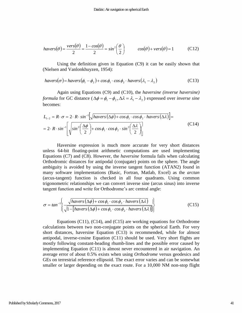
122

1

2

2

verscossin

cosvershavers (C12)

Using the definition given in Equation (C9) it can be easily shown that

(Nielsen and Vanlonkhuyzen, 1954):

212121 haverscoscoshavershavers (C13)

Again using Equations (C9) and (C10), the haversine (inverse haversine)

formula for GC distance ( 2121 , ) expressed over inverse sine

becomes:

222

2

2

21

21

21

1

21

sincoscossinsinR

haverscoscoshaverssinRRL

(C14)

Haversine expression is much more accurate for very short distances

unless 64-bit floating-point arithmetic computations are used implementing

Equations (C7) and (C8). However, the haversine formula fails when calculating

Orthodromic distances for antipodal (conjugate) points on the sphere. The angle

ambiguity is avoided by using the inverse tangent function (ATAN2) found in

many software implementations (Basic, Fortran, Matlab, Excel) as the arctan

(arcus-tangent) function is checked in all four quadrants. Using common

trigonometric relationships we can convert inverse sine (arcus sinus) into inverse

tangent function and write for Orthodrome’s arc central angle:

haverscoscoshavers

haverscoscoshaverstan

21

211

1 (C15)

Equations (C11), (C14), and (C15) are working equations for Orthodrome

calculations between two non-conjugate points on the spherical Earth. For very

short distances, haversine Equation (C13) is recommended, while for almost

antipodal, inverse-cosine Equation (C11) should be used. Very short flights are

mostly following constant-heading rhumb-lines and the possible error caused by

implementing Equation (C11) is almost never encountered in air navigation. An

average error of about 0.5% exists when using Orthodrome versus geodesics and

GEs on terrestrial reference ellipsoid. The exact error varies and can be somewhat

smaller or larger depending on the exact route. For a 10,000 NM non-stop flight

41



one can expect an error typically of about 30-50 NM (corresponding to 4-6

minutes in high-altitude high-subsonic cruise flight), which is acceptable for most

applications considering all other uncertainties. To reduce distance errors to

0.05%, or less, GE on oblate ellipsoidal Earth approximation is recommended

(Bowring, 1984; Sjöberg, 2012; Tseng and Lee, 2010). Accurate geodesic

distances from few centimeters to 20,000 km on WGS-84 reference ellipsoids can

be calculated using the well-known iterative algorithm of Vincenty (1975) and

Karney (2013), but for air navigation purposes this is hardly needed.

To calculate all (or arbitrary many) waypoints on the GC, we use the

normal vector on the osculating plane in which GC lies. Using the definition of

the vector (or cross) product, we obtain the vector normal as (Ayres as

Mendelson, 2009; Bronstein and Semendjajew, 1989; Hall, 1968; Olza et al.,

1974; Wolper, 2001):

122121121221

222

11121

yxyxzxzxzyzy

NNN

zyx

zyx zyx

kji

kji

kji

rrN (C16)

where,

jikikjkjikkjjii 0

After complicating vector algebra using Equation (C2), we obtain for

normal vector components:

2121

2

121212

2

212121

2

sincoscosRN

cossincoscossincosRN

sinsincossinsincosRN

z

y

x

(C17)

Since vector normal is perpendicular to all points lying on the plane,

including the points that are common to GC, then for an arbitrary vector point on

an Orthodrome, we write the condition for perpendicularity of vectors:

0 zNyNxN zyxrN (C18)

By substituting the spherical coordinates from Equation (C2), we obtain:

42



z

yx

z

yx

N

sinNcosNtan

N

sinNcosNtan

1 (C19)

Thus any point on a GC segment must satisfy Equations (B15) and (C19).

After substituting Equation (C17) into Equation (C19), we obtain latitude on a GC

for an arbitrary longitude (taken between the starting and ending longitudes):

21

21

12211

sin

sintansintantan (C20)

The heading (TC) is constantly changing on GC route (unless on

meridians or equator). This is due to convergence of meridians ( sin )

toward the poles which can be observed in Figure C2. Small circle radii decrease

with the cosine of latitude to become zero at the poles (see Equation A10 and its

corollaries). Also shown in Figure C2 is Loxodrome, which is curving toward

nearest pole. As a matter of fact, the Loxodrome would be spiraling infinitely

around the pole, but has a finite length.

Figure C2. Gnomonic projection depicting Orthodrome and Loxodrome. Not to

scale.

43



Using the Law of Sines in spherical trigonometry (Bronstein and

Semendjajew, 1989; Danby, 1962; Nielsen and Vanlonkhuyzen, 1954; Olza et al.,

1974; Spiegel and Liu, 1999; Todhunter, 1886), we can write:

2

1

2

1

1

2

sin

sin

sin

sin

sin

sin

sin

sin

(C21)

The starting and ending (final) true courses (heading or bearing) are:

1

1

22

1

1

cos

sin

sinsincos

sin

sinsin (C22)

Unfortunately, this simple relationship does not resolve angle ambiguity of

inverse-sine and is quite dangerous to implement trivially. But the TC information

can be also obtained using the Cosine Law of spherical trigonometry (Danby,

1962; Nielsen and Vanlonkhuyzen, 1954; Todhunter, 1886), resulting in:

sincos

cossinsincoscos

sincos

cossinsin

sinsin

coscoscoscos

2

21

22

1

12

1

12

1

(C23)

For numerical accuracy and resolving the angle ambiguity using periodic

trigonometric functions it is always better to use inverse-tangent function which

in software implementation is typically coded as ATAN2(y,x) or similar (in True

Basic an intrinsic function ANGLE (x,y) is used). Quadrants are shown in Figure

C3. In terms of inverse tangent function by combining Equations (C22) and (C23)

and doing basic trigonometric transformations, one obtains (see Figures C2 and

C3):

22

212

1

2

121

1

1

cossintancos

sintan

cossintancos

sintan

(C24)

Utilizing the Law of Sines, we can also find the very important point along

GC route called the vertex (Jeppesen, 2007; Underdown and Palmer, 2001;

Wolper, 2001). Vertex is the point of highest latitude (N or S) for which the

44



instantaneous TC is equal to 90 o or 270o and is illustrated in Figure C3 together

with the GC segments. Using the Law of Sines as given in Equation (C21), we can

write from the second and third equality:

2211

2

1

1

2

cossincossin

sin

sin

sin

sin

(C25)

Figure C3. The location of vertex on GC-arc routes using the polar gnomonic

projection. Not to scale.

This expression is sometimes called Clairaut’s relation or theorem (Struik,

1988), but for spheres it actually comes originally from many Arabic and

Iranian/Persian scholars in the period from 9th to 13th century, such as, Al-Jayyani

and Nasir al-din al-Tusi (Struik, 1987) who, by-the-way, have fully developed

planar and spherical trigonometry. Equation (C25) is valid for any two points on a

GC. It will also be valid for the point where the GC crosses equator (going N or

S). Since the latitude at the equator is 0o, and the TC at vertex is 12 sin or

123 sin , we may write:

vertexeq coscossincossinsin 2211 (C26)

45



The latitude (N or S) of the vertex is thus:

cossincoscossincossincos eqvertex 1

11

11 (C27)

A GC which is not an equator or meridian (with anti-meridian) will have

two vertices (“higher” and “lower” or N and S). The longitude of the vertex is

shifted by 90o from the longitude at which GC crosses Equator. The longitude of

the vertex can be easily derived and yields:

vertex

vertextan

tancos

11

1 (C28)

We can easily prove the relationship between the vertex and Equator’s

(Eq) crossing longitudes by using:

vertexvertexEqEq tancostan (C29)

All vertex geometric properties can be derived using Napier’s rules of

right-angled spherical triangle (Bowditch, 2002; Nielsen and Vanlonkhuyzen,

1954; Olza et al., 1974; Todhunter, 1886). Since Equator is excluded as a GC

route and has undefined vertex it must be 0vertextan . On the other hand, we

have 0Eqtan . Hence the solution is:

,,,nncos vertexEqvertexEq 2102

120

(C30)

Finally, we have defined and derived all working equations necessary for

GC route computations on spherical Earth. In general, if the Orthodrome route is

along the equator or any meridian (which are GCs on spherical Earth) then the

problem is trivial and many of the here derived equations will fail. For example,

vertex is undefined for the GC along the Equator or any meridian. However, the

TCs are then simply equal to 0o/180o (along any meridian) or 90o /270o (along

Equator) and the Orthodrome is equal to change in longitude multiplied by the

spherical Earth radius (6,371 km) when along equator. Similar reasoning will

apply for any meridian and its anti-meridian.

46



Appendix D

Short distance Great Circle navigation on a perfect sphere

As mentioned previously the cosine-formula for GC (Equation C8) fails for very

short arcs. While mathematically exact, the problem occurs with the finite number

of digits representation as was illustrated by Sinnott (1984). Essentially for

angular distances of less than 1 arc-minute it is better to use haversine formula

(Equations C14 and C15) although modern 64-bit floating point arithmetic’s can

push the envelope to less than 1 arc-second. Such small angular distances have

important astronomical, but practically no air navigation applications.

For short distances on Earth (around 20 km or less), it is acceptable to

neglect Earth’s spheroidal shape and utilize planar-trigonometry. Here, we will

distinguish two special cases (1) Polar-coordinates flat-Earth formula used with

polar azimuthal projections for high latitudes, and (2) planar projections using

simple Pythagoras theorem (Euclidian space). Close to the geographic poles (NP

or SP), the polar projections (De Remer and McLean, 1998; Jeppesen, 2007;

Struik, 1988; Underdown and Palmer, 2001) will result in meridians being

represented as radials coming out of poles, while the lines of latitude are

concentric circles with separation distance between them changing depending on

the type of projection. The polar stereographic azimuthal projections is illustrated

in Figure D1. Polar gnomonic would be very similar, but the distance between the

lines of latitude will be increasing rapidly (Equator is in infinity). Orthographic

projection has center of projection in infinity (Figure D2). The lines of latitude are

decreasingly spaced concentric circles. Conjugate hemisphere is not represented.

Figure D1. Polar stereographic azimuthal projection of Earth. Not to scale.

47



Figure D2. Polar orthographic azimuthal (plane) projection of Earth. Not to scale.

Polar-coordinates azimuthal projection formula originates from the Law of

Cosines of planar trigonometry (Olza et al, 1974; Spiegel and Liu, 1999) as

illustrated in Figure D3:

2

2 2121

2

2

2

121

cos (D1)

Figure D3. Polar azimuthal gnomonic projection with polar coordinates and

rectangular azimuthal projection for short-distance computations.

Substituting co-latitudes (polar distances) with geocentric latitudes, we

obtain for the central angle and the chord distance approximating GC arc:

48



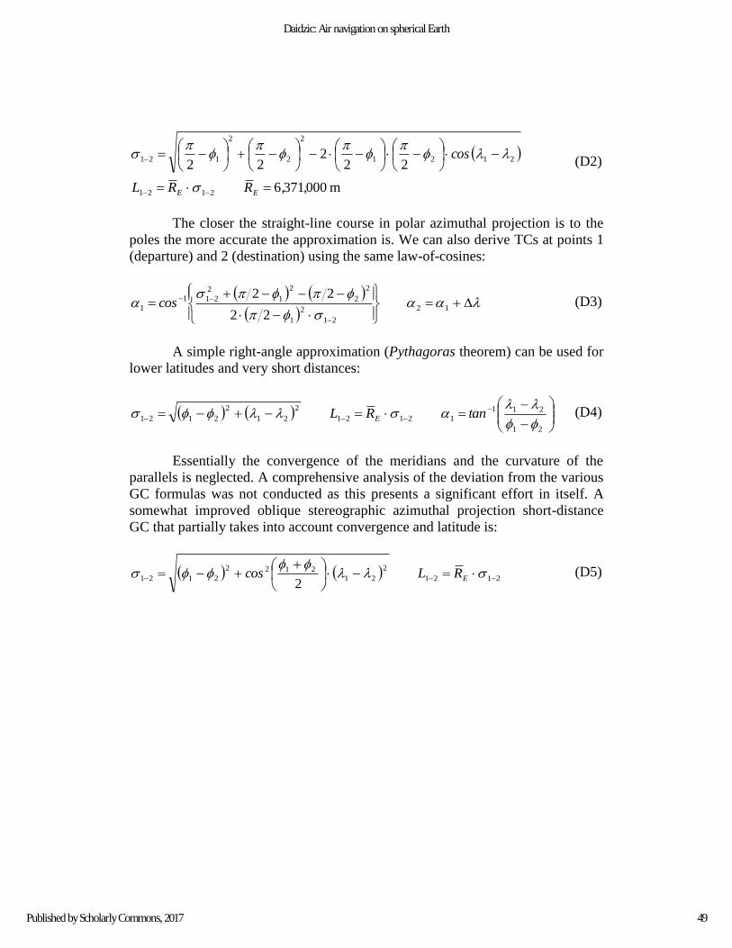
m0003716

222

22

2121

2121

2

2

2

121

,,RRL

cos

EE

(D2)

The closer the straight-line course in polar azimuthal projection is to the

poles the more accurate the approximation is. We can also derive TCs at points 1

(departure) and 2 (destination) using the same law-of-cosines:

12

21

2

1

2

2

2

1

2

211

122

22cos (D3)

A simple right-angle approximation (Pythagoras theorem) can be used for

lower latitudes and very short distances:

21

211

12121

2

21

2

2121

tanRL E

(D4)

Essentially the convergence of the meridians and the curvature of the

parallels is neglected. A comprehensive analysis of the deviation from the various

GC formulas was not conducted as this presents a significant effort in itself. A

somewhat improved oblique stereographic azimuthal projection short-distance

GC that partially takes into account convergence and latitude is:

2121

2

21

2122

21212

ERLcos (D5)

49



Appendix E

Rhumb line navigation and the Loxodrome

Maintaining constant angle (headings, courses, bearings) in relationship to

terrestrial meridians is called rhumb-line navigation. Rhumbs are part of curves

called Loxodromes. Rhumb line navigation does not deliver shortest distances on

spherical or spheroidal Earth. A Loxodrome is a very interesting curve that for

any heading other than North-South and East-West (coincides with Orthodromes)

ends up spiraling around the NP and SP (Alexander, 2004; Lipshutz, 1969; Struik,

1988). Loxodrome is a straight line on a Mercator cylindrical conformal

projection. For example, on a polar stereographic conformal projection a

Loxodrome becomes a logarithmic spiral (Lipshutz, 1969; Struik, 1988;

Alexander, 2004) about respective poles. Conformal Mercator cylindrical chart

provides for uniform stretching throughout the chart (N-S and E-W) resulting in

preservation of local angles (conformality) delivering isotropic Representative

Fraction (RF) or scale. The local and the total stretching from the Equator on

spherical Earth is expressed mathematically as:

42

1

0

tanlntanseclndsec

cossec

(E1)

The method of calculating total stretching in the medieval time was de-

facto numerical integration and was referred to by Edward Wright as “perpetual

addition of Secants” (Alexander, 2004). Naturally for Mercator cylindrical

projections with the line of contact coinciding with the Equator, the poles

(singular points on sphere) cannot be represented as the total stretching goes to

infinity. One could use oblique or transverse cylindrical projections instead to

depict poles (De Remer and McLean, 1998; Jeppesen, 2007; Underdown and

Palmer, 2001).

Using Equation (A11) with one vector being collinear with the lines of

longitude ( 0 .,const ), while the other represents Loxodrome on a

sphere, one obtains:

REs

ds

dR

sds

dEcos 2 (E2)

50



Using the first fundamental form for sphere this can be written as:

dctg

cos

ddRdscos 2222 (E3)

Integrating Equation (E3), we obtain:

.constctgmctgdctgcos

d

12

2

1

2

1

And finally using Equation (E1):

1212

4242

ctgtanlntanln (E4)

This leads to a constant course or bearing between two points connected

by a Loxodrome on Mercator chart:

42

1

12

12

tanlnM

mMMtan (E5)

Here, M’s are called meridional parts (mer-parts) for respective latitudes

(Williams, 1950). Loxodromic distance can be easily calculated using the

knowledge of differential geometry (Lipshutz, 1969; Struik, 1988). Employing

Equation (A10), the arc-length of Loxodrome part becomes:

secRcos

Rdd

dcosRL

12

12

212

2

21

2

1

1 (E6)

Since,

sectan

cos

tan

d

d

, where

20

.

As the TC angle (measured from TN) approaches 90o (but not 90o itself)

the Loxodrome length sharply increases. Kos et al. (1999) obtained similar result

utilizing co-latitudes and using similar differential geometry arguments. However,

by not using absolute value of co-latitude differences their Loxodrome distance

can become negative. Alexander (2004) derived Loxodrome distance using:

51



secRdd

d

d

dRL

12

2

221

2

1

11 (E7)

where from Equation (E1):

tan

d

dsec

d

d

A practical expression for constant TC (bearing) rhumb line navigation

between two points on spherical Earth is now:

42

42

1

2

12

1

tan

tanlntan (E8)

One has to be careful when the Loxodrome is crossing Greenwich anti-

meridian or approximately the International Date Line (IDL). Conformal

Mercator chart can be easily constructed by using X and Y coordinates as (Struik,

1988):

420

tanlnRYRX EE

(E9)

Loxodromes on an ellipsoidal Earth can be also easily calculated in which

case the stretching has to include the eccentricity (Alexander, 2004; Bennett, G.

G., 1996; Williams, 1950). The latitudes of the corresponding mer-parts are:

2

2 1 MexptanM (E10)

Although the Loxodrome is a curve spiraling infinitely around the SP and

the NP, the distance is always finite except for angle of 90o (cos π = 0):

0

80010NM

cos

,

cos

RL NPSP (E11)

52



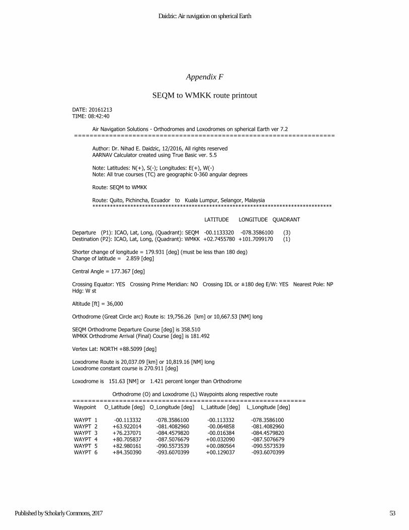
Appendix F

SEQM to WMKK route printout DATE: 20161213 TIME: 08:42:40 Air Navigation Solutions - Orthodromes and Loxodromes on spherical Earth ver 7.2 =================================================================== Author: Dr. Nihad E. Daidzic, 12/2016, All rights reserved AARNAV Calculator created using True Basic ver. 5.5 Note: Latitudes: N(+), S(-); Longitudes: E(+), W(-) Note: All true courses (TC) are geographic 0-360 angular degrees Route: SEQM to WMKK Route: Quito, Pichincha, Ecuador to Kuala Lumpur, Selangor, Malaysia ********************************************************************************** LATITUDE LONGITUDE QUADRANT Departure (P1): ICAO, Lat, Long, (Quadrant): SEQM -00.1133320 -078.3586100 (3) Destination (P2): ICAO, Lat, Long, (Quadrant): WMKK +02.7455780 +101.7099170 (1) Shorter change of longitude = 179.931 [deg] (must be less than 180 deg) Change of latitude = 2.859 [deg] Central Angle = 177.367 [deg] Crossing Equator: YES Crossing Prime Meridian: NO Crossing IDL or ±180 deg E/W: YES Nearest Pole: NP Hdg: W st Altitude [ft] = 36,000 Orthodrome (Great Circle arc) Route is: 19,756.26 [km] or 10,667.53 [NM] long SEQM Orthodrome Departure Course [deg] is 358.510 WMKK Orthodrome Arrival (Final) Course [deg] is 181.492 Vertex Lat: NORTH +88.5099 [deg] Loxodrome Route is 20,037.09 [km] or 10,819.16 [NM] long Loxodrome constant course is 270.911 [deg] Loxodrome is 151.63 [NM] or 1.421 percent longer than Orthodrome Orthodrome (O) and Loxodrome (L) Waypoints along respective route ============================================================ Waypoint O_Latitude [deg] O_Longitude [deg] L_Latitude [deg] L_Longitude [deg] WAYPT 1 -00.113332 -078.3586100 -00.113332 -078.3586100 WAYPT 2 +63.922014 -081.4082960 -00.064858 -081.4082960 WAYPT 3 +76.237071 -084.4579820 -00.016384 -084.4579820 WAYPT 4 +80.705837 -087.5076679 +00.032090 -087.5076679 WAYPT 5 +82.980161 -090.5573539 +00.080564 -090.5573539 WAYPT 6 +84.350390 -093.6070399 +00.129037 -093.6070399

53



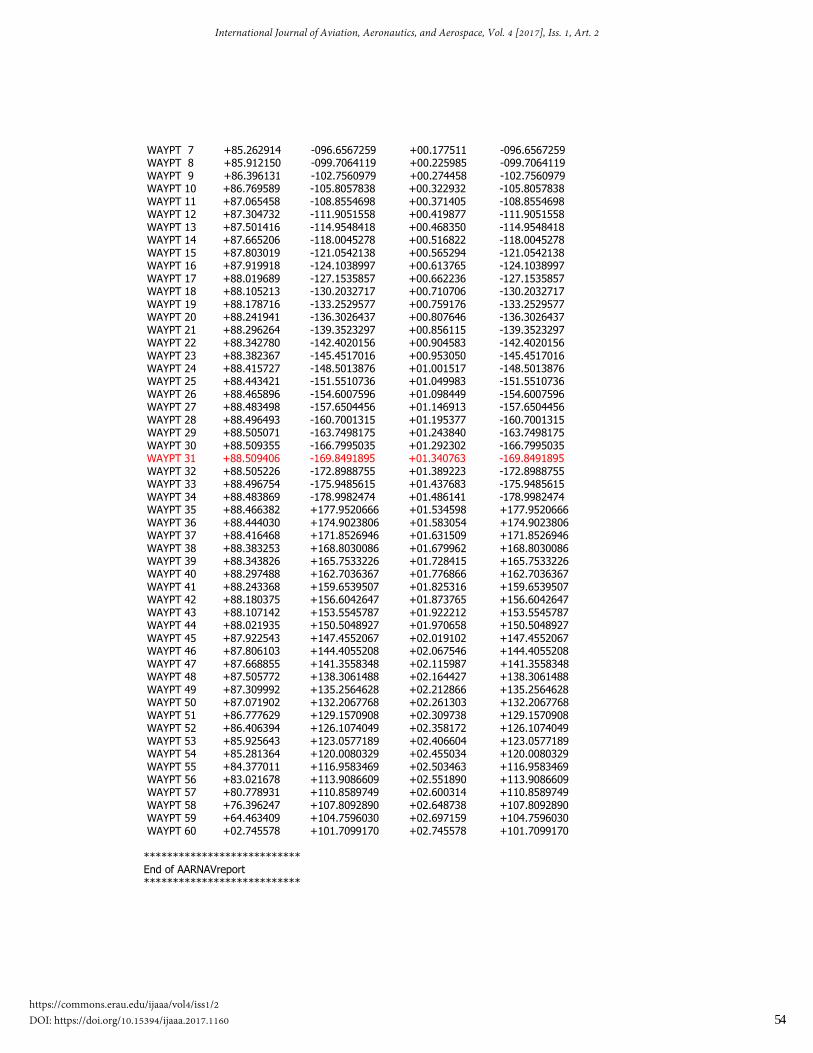
WAYPT 7 +85.262914 -096.6567259 +00.177511 -096.6567259 WAYPT 8 +85.912150 -099.7064119 +00.225985 -099.7064119 WAYPT 9 +86.396131 -102.7560979 +00.274458 -102.7560979 WAYPT 10 +86.769589 -105.8057838 +00.322932 -105.8057838 WAYPT 11 +87.065458 -108.8554698 +00.371405 -108.8554698 WAYPT 12 +87.304732 -111.9051558 +00.419877 -111.9051558 WAYPT 13 +87.501416 -114.9548418 +00.468350 -114.9548418 WAYPT 14 +87.665206 -118.0045278 +00.516822 -118.0045278 WAYPT 15 +87.803019 -121.0542138 +00.565294 -121.0542138 WAYPT 16 +87.919918 -124.1038997 +00.613765 -124.1038997 WAYPT 17 +88.019689 -127.1535857 +00.662236 -127.1535857 WAYPT 18 +88.105213 -130.2032717 +00.710706 -130.2032717 WAYPT 19 +88.178716 -133.2529577 +00.759176 -133.2529577 WAYPT 20 +88.241941 -136.3026437 +00.807646 -136.3026437 WAYPT 21 +88.296264 -139.3523297 +00.856115 -139.3523297 WAYPT 22 +88.342780 -142.4020156 +00.904583 -142.4020156 WAYPT 23 +88.382367 -145.4517016 +00.953050 -145.4517016 WAYPT 24 +88.415727 -148.5013876 +01.001517 -148.5013876 WAYPT 25 +88.443421 -151.5510736 +01.049983 -151.5510736 WAYPT 26 +88.465896 -154.6007596 +01.098449 -154.6007596 WAYPT 27 +88.483498 -157.6504456 +01.146913 -157.6504456 WAYPT 28 +88.496493 -160.7001315 +01.195377 -160.7001315 WAYPT 29 +88.505071 -163.7498175 +01.243840 -163.7498175 WAYPT 30 +88.509355 -166.7995035 +01.292302 -166.7995035 WAYPT 31 +88.509406 -169.8491895 +01.340763 -169.8491895 WAYPT 32 +88.505226 -172.8988755 +01.389223 -172.8988755 WAYPT 33 +88.496754 -175.9485615 +01.437683 -175.9485615 WAYPT 34 +88.483869 -178.9982474 +01.486141 -178.9982474 WAYPT 35 +88.466382 +177.9520666 +01.534598 +177.9520666 WAYPT 36 +88.444030 +174.9023806 +01.583054 +174.9023806 WAYPT 37 +88.416468 +171.8526946 +01.631509 +171.8526946 WAYPT 38 +88.383253 +168.8030086 +01.679962 +168.8030086 WAYPT 39 +88.343826 +165.7533226 +01.728415 +165.7533226 WAYPT 40 +88.297488 +162.7036367 +01.776866 +162.7036367 WAYPT 41 +88.243368 +159.6539507 +01.825316 +159.6539507 WAYPT 42 +88.180375 +156.6042647 +01.873765 +156.6042647 WAYPT 43 +88.107142 +153.5545787 +01.922212 +153.5545787 WAYPT 44 +88.021935 +150.5048927 +01.970658 +150.5048927 WAYPT 45 +87.922543 +147.4552067 +02.019102 +147.4552067 WAYPT 46 +87.806103 +144.4055208 +02.067546 +144.4055208 WAYPT 47 +87.668855 +141.3558348 +02.115987 +141.3558348 WAYPT 48 +87.505772 +138.3061488 +02.164427 +138.3061488 WAYPT 49 +87.309992 +135.2564628 +02.212866 +135.2564628 WAYPT 50 +87.071902 +132.2067768 +02.261303 +132.2067768 WAYPT 51 +86.777629 +129.1570908 +02.309738 +129.1570908 WAYPT 52 +86.406394 +126.1074049 +02.358172 +126.1074049 WAYPT 53 +85.925643 +123.0577189 +02.406604 +123.0577189 WAYPT 54 +85.281364 +120.0080329 +02.455034 +120.0080329 WAYPT 55 +84.377011 +116.9583469 +02.503463 +116.9583469 WAYPT 56 +83.021678 +113.9086609 +02.551890 +113.9086609 WAYPT 57 +80.778931 +110.8589749 +02.600314 +110.8589749 WAYPT 58 +76.396247 +107.8092890 +02.648738 +107.8092890 WAYPT 59 +64.463409 +104.7596030 +02.697159 +104.7596030 WAYPT 60 +02.745578 +101.7099170 +02.745578 +101.7099170 *************************** End of AARNAVreport ***************************

54



Long and short-range air navigation on spherical Earth

Documents

Transcript of Long and short-range air navigation on spherical Earth