1

Logic-based Modeling and Solution of Nonlinear Discrete/Continuous

Optimization Problems

Sangbum Lee and Ignacio E. Grossmann∗

Department of Chemical Engineering

Carnegie Mellon University

Pittsburgh, PA15213

November 28, 2003

(submitted to Annals of Operations Research)

Abstract

This paper presents a review of advances in the mathematical programming approach to

discrete/continuous optimization problems. We first present a brief review of MILP and MINLP for the

case when these problems are modeled with algebraic equations and inequalities. Since algebraic

representations have some limitations such as difficulty of formulation and numerical singularities for the

nonlinear case, we consider logic -based modeling as an alternative approach, particularly Generalized

Disjunctive Programming (GDP), which the authors have extensively investigated over the last few years.

Solution strategies for GDP models are reviewed, including the continuous relaxation of the disjunctive

constraints. Also, we briefly review a hybrid model that integrates disjunctive programming and mixed-

integer programming. Finally, the global optimization of nonconvex GDP problems is discussed through

a two-level branch and bound procedure.

Keywords : mixed-integer programming, generalized dis junctive programming, global optimization,

logic-based programming

1. Introduction

The mathematical programming approach to discrete/continuous optimization problems has been

widely used in operations research and engineering. For example, the applications are in process design

and synthesis, planning and scheduling, process control, and recently, in bioinformatics. Over the last

decades, there has been a significant progress in the development of the discrete/continuous optimization

models and their solution algorithms. For a recent review in the applications to the process systems

engineering, see Grossmann et al. (1999). It is the objective of this paper to present an overview of the

major advances in the mathematical programming techniques for the modeling and solution of

∗ To whom all correspondence should be addressed. Tel.: 412-268-2230, Fax: 412-268-7139 Email: grossmann@cmu.edu

2

discrete/continuous optimization problems. This paper is organized as follows. First, the modeling

formulations and their solution strategies are presented. We then briefly review the continuous relaxation

of discrete/continuous models. Finally, a global optimization method of nonconvex problems will be

presented. Also, the possibilities of the hybrid model of mixed-integer program and disjunctive program

are discussed.

2. Review of Mixed Integer Optimization

The conventional way of modeling discrete/continuous optimization problems has been through the use of

0-1 and continuous variables, and algebraic equations and inequalities. For the case of linear functions

this model corresponds to a mixed-integer linear programming (MILP) model, which has the following

general form,

mn

TT

yRx

d BxAytsxbyaZ

1,0 ,

(MILP) .. min

∈∈

≤++=

In problem (MILP) the variables x are continuous, and y are discrete variables, which generally are

binary variables. As is well known, problem (MILP) is NP-hard. Nevertheless, an interesting theoretical

result is that it is possible to transform it into an LP with the convexification procedures proposed by

Lovacz and Schrijver (1991), Sherali and Adams (1990), and Balas et al (1993). These procedures consist

in sequentially lifting the original relaxed x-y space into higher dimension and projecting it back to the

original space so as to yield after a finite number of steps the integer convex hull. Since the number of

operations required is exponential, these procedures are only of theoretical interest, although they can be

used as a basis for deriving cutting planes (e.g. lift and project method by Balas et al, 1993).

As for the solution of problem (MILP), it should be noted that this problem becomes an LP problem

when the binary variables are relaxed as continuous variables, 0 ≤ y ≤ 1. The most common solution

algorithms for problem (MILP) are LP-based branch and bound methods, which are enumeration methods

that solve LP subproblems at each node of the search tree. This technique was initially conceived by Land

and Doig (1960), Balas (1965), and later formalized by Dakin, (1965). Cutting plane techniques, which

were initially proposed by Gomory (1958), and consist of successively generating valid inequalities that

are added to the relaxed LP, have received renewed interest through the works of Crowder et al (1983),

Van Roy and Wolsey (1986), and especially the lift and project method of Balas et al (1993). A recent

review of branch and cut methods can be found in Johnson et al. (2000). Finally, Benders decomposition

(Benders, 1962) is another technique for solving MILPs in which the problem is successively

decomposed into LP subproblems for fixed 0-1 and a master problem for updating the binary variables.

3

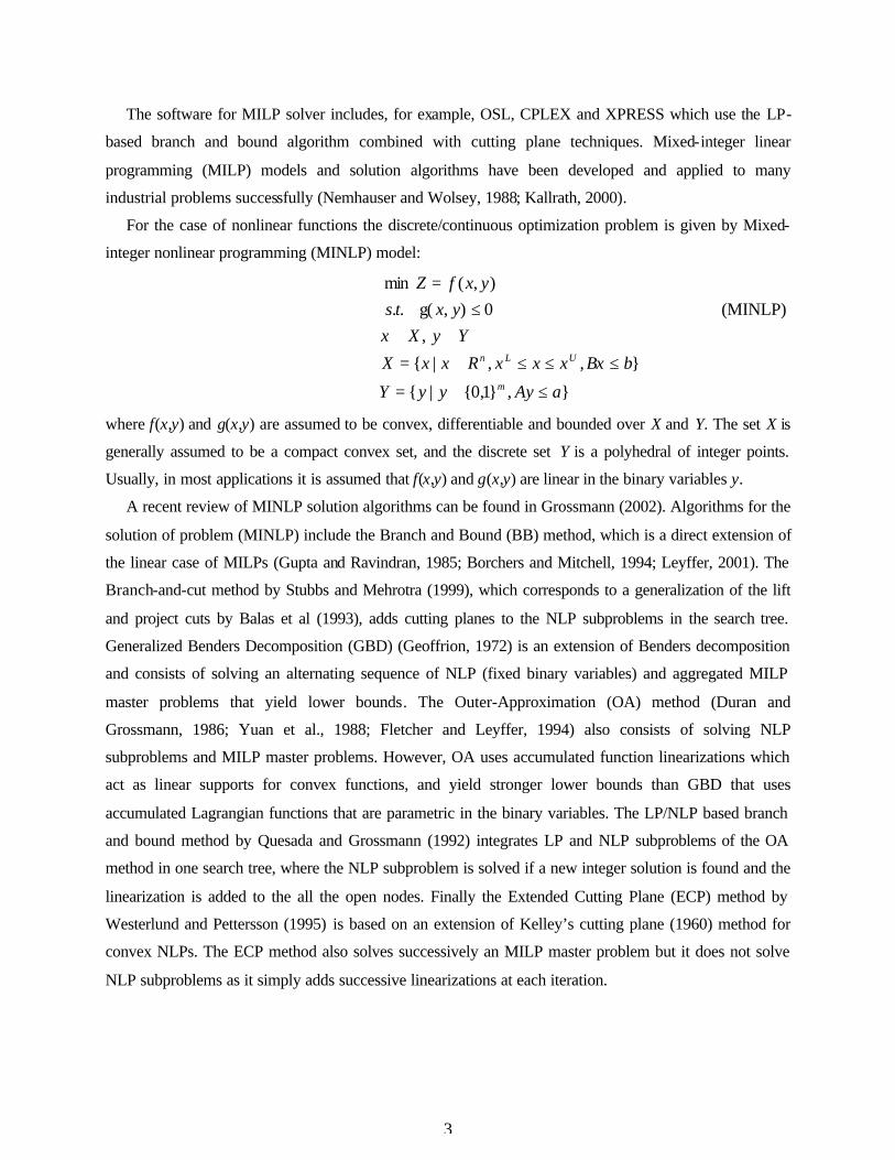
The software for MILP solver includes, for example, OSL, CPLEX and XPRESS which use the LP-

based branch and bound algorithm combined with cutting plane techniques. Mixed-integer linear

programming (MILP) models and solution algorithms have been developed and applied to many

industrial problems successfully (Nemhauser and Wolsey, 1988; Kallrath, 2000).

For the case of nonlinear functions the discrete/continuous optimization problem is given by Mixed-

integer nonlinear programming (MINLP) model:

,1,0|

,,|

,(MINLP) 0),g( ..

),( min

aAyyyY

bBxxxxRxxX

YyXx yxts

yxfZ

m

ULn

≤∈=

≤≤≤∈=

∈∈≤

=

where f(x,y) and g(x,y) are assumed to be convex, differentiable and bounded over X and Y. The set X is

generally assumed to be a compact convex set, and the discrete set Y is a polyhedral of integer points.

Usually, in most applications it is assumed that f(x,y) and g(x,y) are linear in the binary variables y.

A recent review of MINLP solution algorithms can be found in Grossmann (2002). Algorithms for the

solution of problem (MINLP) include the Branch and Bound (BB) method, which is a direct extension of

the linear case of MILPs (Gupta and Ravindran, 1985; Borchers and Mitchell, 1994; Leyffer, 2001). The

Branch-and-cut method by Stubbs and Mehrotra (1999), which corresponds to a generalization of the lift

and project cuts by Balas et al (1993), adds cutting planes to the NLP subproblems in the search tree.

Generalized Benders Decomposition (GBD) (Geoffrion, 1972) is an extension of Benders decomposition

and consists of solving an alternating sequence of NLP (fixed binary variables) and aggregated MILP

master problems that yield lower bounds. The Outer-Approximation (OA) method (Duran and

Grossmann, 1986; Yuan et al., 1988; Fletcher and Leyffer, 1994) also consists of solving NLP

subproblems and MILP master problems. However, OA uses accumulated function linearizations which

act as linear supports for convex functions, and yield stronger lower bounds than GBD that uses

accumulated Lagrangian functions that are parametric in the binary variables. The LP/NLP based branch

and bound method by Quesada and Grossmann (1992) integrates LP and NLP subproblems of the OA

method in one search tree, where the NLP subproblem is solved if a new integer solution is found and the

linearization is added to the all the open nodes. Finally the Extended Cutting Plane (ECP) method by

Westerlund and Pettersson (1995) is based on an extension of Kelley’s cutting plane (1960) method for

convex NLPs. The ECP method also solves successively an MILP master problem but it does not solve

NLP subproblems as it simply adds successive linearizations at each iteration.

4

3. Generalized Disjunctive Programming

In recent years the following major approaches have emerged for solving discrete/continuous

optimization problems with logic -based techniques: Generalized Disjunctive Programming (GDP)

(Raman and Grossmann, 1994), Mixed Logic Linear Programming (MLLP) (Hooker and Osorio, 1999),

and Constraint Programming (CP) (Hentenryck, 1989) The motivations for these logic -based modeling

has been to facilitate the modeling, reduce the combinatorial search effort, and improve the handling the

nonlinearities. In this paper we will concentrate on Generalized Disjunctive Programming. A general

review of logic-based optimization can be found in Hooker (1999).

Generalized Disjunctive Programming (GDP) (Raman and Grossmann, 1994) is an extension of

disjunctive programming (Balas, 1979) that provides an alternate way of modeling (MILP) and (MINLP)

problems. The general formulation of a (GDP) is as follows:

mmn

jkk

jk

jk

k

Kkk

falsetrueYRcRx

TrueY

K k

c

xh

Y

Jj

xgts

xfcZ

, , ,

)(

(GDP) , 0)(

0)( ..

)( min

∈∈∈

=Ω

∈

=

≤∈

≤

+=

∨

∑∈

γ

where Yjk are the Boolean variables that decide whether a given term j in a disjunction k ∈ K is true or

false, and x are the continuous variables. The objective function involves the term f(x) for the continuous

variables and the charges ck that depend on the discrete choices in each disjunction k ∈ K. The constraints

g(x) ≤ 0 must hold regardless of the discrete choice, and hjk(x) ≤ 0 are conditional constraints that must

hold when Yjk is true in the j-th term of the k-th disjunction. The cost variables ck correspond to the fixed

charges, and their value equals to γjk if the Boolean variable Yjk is true. Ω(Y) are logical relations for the

Boolean variables expressed as propositional logic.

It should be noted that problem (GDP) can be reformulated as an MINLP problem by replacing the

Boolean variables by binary variables yjk,

5

KkJjyxx

a Ay

Kky

K kJjyMxhxgts

xfyZ

kjkU

Jjjk

kjkjkjk

Kk Jjjkjk

k

k

∈∈∈≤≤

≤

∈=

∈∈−≤≤

+=

∑

∑ ∑

∈

∈ ∈

,, 1,0 ,0

,1

(BM) ,, )1()( 0)( ..

)( min γ

where the disjunctions are replaced by “Big-M” constraints which involve a parameter Mjk and binary

variables yjk. The propositional logic statements Ω(Y) = True are replaced by the linear constraints Ay ≤ a

as described by Williams (1985) and Raman and Grossmann (1991). Here we assume that x is a non-

negative variable with finite upper bound xU. An important issue in model (BM) is how to specify a valid

value for the Big-M parameter Mjk. If the value is too small, then feasible points may be cut off. If Mjk is

too large, then the continuous relaxation might be too loose yielding poor lower bounds. Therefore,

finding the smallest valid value for Mjk is the desired selection. For linear constraints, one can use the

upper and lower bound of the variable x to calculate the maximum value of each constraint, which then

can be used to calculate a valid value of Mjk. For nonlinear constraints one can in principle maximize each

constraint over the feasible region, which is a non-trivial calculation.

4. Convex Hull Relaxation of Disjunction

Lee and Grossmann (2000) have derived the convex hull relaxation of problem (GDP). The basic idea is

as follows. Consider a disjunction k ∈ K that has convex constraints,

0 0

(DP) 0)(

≥≤≤

=

≤∈∨

,cxx

c

xh

Y

U

jk

jk

jk

kJjγ

where hjk(x) are assumed to be convex and bounded over x. The convex hull relaxation of disjunction

(DP), which is an extension of the work by Stubbs and Mehrotra (1999), is given as follows:

6

kjk

kjkjk

jkjk

kjkJj

jk

kjkU

jkjk

Jjjkjk

Jj

jk

Jj?cx

Jj?h

Jj10

Jjx?0

c?x

k

k

∈≥

∈≤

∈≤≤=

∈≤≤

==

∑

∑∑

∈

∈∈

,

,

,

,

0,,

0)/(

(CH),1

,

λλ

λλ

λ

γλ

where vjk are disaggregated variables that are assigned to each term of the disjunction k ∈ K, and λjk are

the weight factors that determine the feasibility of the disjunctive term. Note that when λjk is 1, then the

j’th term in the k’th disjunction is enforced and the other terms are ignored. The constraints

)/( jkjk

jkjk vh λλ are convex if hjk(x) is convex as discussed on p. 160 in Hiriart-Urruty and

Lemaréchal (1993). A formal proof can be found in Stubbs and Mehrotra (1999). Note that the convex

hull (CH) reduces to the result by Balas (1985) if the constraints are linear. Based on the convex hull

relaxation (CH), Lee and Grossmann (2000) proposed the following convex relaxation program of (GDP).

Kk,Jjx?x

aA

Kk,Jjh

Kk,Jjx

K k,?x

xgts

xfZmin

kjkUjk

kjkjk

jkjk

kjkU

jkjk

Jjjk

Jj

jk

Kk Jjjkjk

L

kk

k

∈∈≤≤≤≤

≤

∈∈≤

∈∈≤≤

∈==

≤

+=

∑∑

∑ ∑

∈∈

∈ ∈

,

,10,,0

,0)/?(

,?0

(CRP) 1

0)(..

)(

λ

λ

λλ

λ

λ

λγ

where U is a valid upper bound for x and v. For computational reasons, the nonlinear inequality is written

as 0=))+/(()+( ελελ jkjk

jkjk vh where ε is a small tolerance. This inequality remains convex if

hjk(x) is a convex function. Note that the number of constraints and variables increases in (CRP)

compared with problem (GDP). Problem (CRP) has a unique optimal solution and it yields a valid lower

bound to the optimal solution of problem (GDP) (Lee and Grossmann, 2000). Problem (CRP) can also be

regarded as a generalization of the relaxation proposed by Ceria and Soares (1999) for a special form of

problem (GDP).

As proved by Lee and Grossmann (2000) problem (CRP) has the useful property that the lower bound

is greater than or equal to the lower bound predicted from the relaxation of problem (BM). The relaxation

7

problem (CRP) can be used as a subproblem to construct a disjunctive branch and bound method to solve

problem (GDP) (Lee and Grossmann, 2000), which exploits the tight lower bound of the convex hull

relaxation program when compared with the Big-M MINLP formulation.

5. Solution Algorithms for GDP

For the linear case of problem (GDP) Beaumont (1991) proposed a branch and bound method which

directly branches on the constraints of the disjunctions where no logic constraints are involved. Also for

the linear case Raman and Grossmann (1994) developed a branch and bound method which solves GDP

problem in hybrid form, by exploiting the tight relaxation of the disjunctions and the tightness of the well-

behaved mixed-integer constraints. Another approach for solving a linear GDP is to replace the

disjunctions either by Big-M constraints or by the convex hull of each disjunction (Balas, 1985; Raman

and Grossmann, 1994)

For the nonlinear case a similar way for solving the problem (GDP) is to reformulate it into the

MINLP by restricting the variables λjk in problem (CRP) to 0-1 values. Alternatively, to avoid introducing

a potentially large number of variables and constraints, the GDP might also be reformulated as the

MINLP problem (BM) by using Big-M parameters. One can then apply standard MINLP solution

algorithms (i.e., branch and bound, OA, GBD, and ECP). In order to strengthen the lower bounds one can

derive cutting planes using the convex hull relaxation (CRP). To generate a cutting plane, the following

separation problem (SP), which is a convex NLP, is solved:

10,,

,1

)SP(,,0)/(

,

0)(..)()()(min ,,

≤≤∈

≤

∈=

∈∈≤

∈=

≤−−=

∑

∑

∈

∈

ikn

ik

Diik

kikikikik

Diik

nBMR

TnBMR

yRx

aAy

Kky

KkDiyhy

Kkx

xgtsxxxxx

k

k

ν

ν

ν

φ

where xRBM,n is the solution of problem (BM) with relaxed 0 ≤ yik ≤ 1. Problem (SP) yields a solution point

x* which belongs to the convex hull of the disjunction and is closest to the relaxation solution xRBM,n. The

most violated cutting plane is then given by,

)1(0*)()*( , ≥−− xxxx TnBMR

The cutting plane in (1) is a facet of the linearized convex hull and thus, a valid inequality for problem

(GDP). Problem (BM) is modified by adding the cutting plane (1) as follows:

8

10,

,1

(CP),,)1()(0)(..

)(min

≤≤∈

≤

≤

∈=

∈∈−≤≤

+=

∑

∑ ∑

∈

∈ ∈

ikn

T

Diik

kikikik

Kk Diikik

yRx

bx

aAy

Kky

KkDiyMxhxgts

xfyZ

k

k

β

γ

where bxT ≤β is the cutting plane (1). Since we add a valid inequality to problem (BM), the lower

bound obtained from problem (CP) is generally tighter than before adding the cutting plane.

This procedure for generating the cutting plane can be used either in a Branch and Cut enumeration

method where a special case is to solve the separation problem (SP) only at the root node, or else it can be

used to strengthen the MINLP problem (BM) before applying methods such as OA, GBD, and ECP. It is

also interesting to note that cutting planes can be derived in the (x,y) space, especially when the objective

function has binary variables y.

Another application of the cutting plane is for a decision if it is advantageous to use the convex hull

formulation for a relaxation of disjunction. If the value of || x* - xRBM,n || is large, then it is an indication

that this is the case. A small difference between x* and xRBM,n would indicate that it might be better to

simply use the Big-M relaxation.

There are also direct approaches for solving problem (GDP). In particular, a disjunctive branch and

bound method can be developed which directly branches on the term in a disjunction using the convex

hull relaxation (CRP) as a basic subproblem (Lee and Grossmann, 2000). Problem (CRP) is solved at the

root node of the search tree. The branching rule is to select the least infeasible term in a disjunction first.

We can then consider a dichotomy where we fix the value λjk = 1 for the disjunctive term that is closest to

being satisfied, and consider on the other hand the convex hull of the remaining terms (λjk = 0).

When all the decision variables λjk are fixed, problem (CRP) yields an upper bound to problem (GDP).

The optimal solution is the best upper bound after closing the gap between the lower and the upper bound.

The proposed algorithm has obviously finite convergence since the number of the terms in the disjunction

is finite. Also, since the nonlinear functions are convex, each subproblem has a unique optimal solution.

Therefore, the rigorous validity of the bounds is guaranteed.

6. Disjunctive Branch and Bound Example

For the illustration of the disjunctive branch and bound algorithm described at the end of Section 5, we

present the following GDP problem with one disjunction:

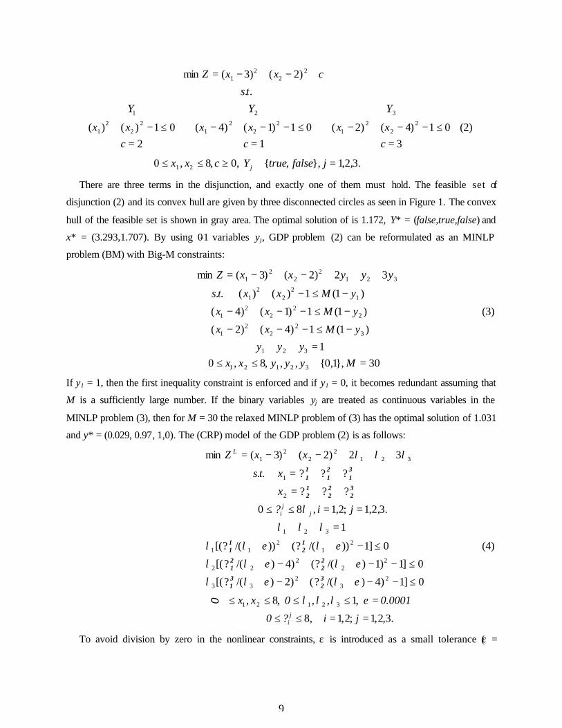
9

.3,2,1,,,0,8,0

(2)3

01)4()2(1

01)1()4(2

01)()(

..

)2()3(min

21

22

21

3

22

21

2

22

21

1

22

21

=∈≥≤≤

=≤−−+−∨

=≤−−+−∨

=≤−+

+−+−=

jfalsetrueYcxx

cxx

Y

cxx

Y

cxx

Y

ts

cxxZ

j

There are three terms in the disjunction, and exactly one of them must hold. The feasible set of

disjunction (2) and its convex hull are given by three disconnected circles as seen in Figure 1. The convex

hull of the feasible set is shown in gray area. The optimal solution of is 1.172, Y* = (false,true,false) and

x* = (3.293,1.707). By using 0-1 variables yj, GDP problem (2) can be reformulated as an MINLP

problem (BM) with Big-M constraints:

30 ,1,0,, ,8, 0 1

)1(1)4()2(

(3) )1(1)1()4(

)1(1)()( ..

32)2()3(min

32121

321

32

22

1

22

22

1

12

22

1

3212

22

1

=∈≤≤=++

−≤−−+−

−≤−−+−

−≤−+

+++−+−=

Myyyxxyyy

yMxx

yMxx

yMxxts

yyyxxZ

If y1 = 1, then the first inequality constraint is enforced and if y1 = 0, it becomes redundant assuming that

M is a sufficiently large number. If the binary variables yj are treated as continuous variables in the

MINLP problem (3), then for M = 30 the relaxed MINLP problem of (3) has the optimal solution of 1.031

and y* = (0.029, 0.97, 1,0). The (CRP) model of the GDP problem (2) is as follows:

.3,2,1;2,1,8

,1,,,8,

0]1)4)/(?()2)/(?([

0]1)1)/(?()4)/(?[(

(4) 0]1))/(?())/(?[(

1

.3,2,1;2,1,80

???

???..

32)2()3(min

32121

23

233

22

222

21

211

321

2

1

3212

22

1

==≤≤

=≤≤≤≤

≤−−++−+

≤−−++−+

≤−+++

=++

==≤≤

++=

++=

+++−+−=

ji?0

0.00010xx

ji?

x

xts

xxZ

ji

jj

i

L

32

31

22

21

12

11

32

22

12

31

21

11

ελλλ

ελελλ

ελελλ

ελελλ

λλλ

λ

λλλ

0

To avoid division by zero in the nonlinear constraints, ε is introduced as a small tolerance (ε =

10

0.0001). The optimal solution of problem (4) is 1.154 and xL = (3.195,1.797). Notice that the lower bound

(1.154) is tighter than the relaxed solution of MINLP problem (3) (1.031). It should be noted that the

convex hull NLP (4) has more variables and constraints than Big-M problem (3). Therefore, the tighter

lower bound comes with the price of increased model size and possibly longer CPU time.

In the disjunctive branch and bound method, λj will be used in deciding which Boolean variable

should be selected at the next node in the search tree. Figure 2 and 3 shows the feasible sets of the

subproblems in the search tree. At the root node, problem (4) yields a lower bound ZL = 1.154. This

solution point xL lies outside the feasible region of GDP problem (2) since xL does not satisfy any term in

the disjunction. In the solution λ2 has the largest value, so we set Y2 as true. At the first node, the GDP

problem is solved with fixed Y = (false,true,false). It means that we fix λ2 as 1 and other λj as 0 in

problem (4). Therefore, the feasible region is restricted to S2 only as shown in Figure 2. Solving GDP

problem (2) with Y2 = true yields an upper bound ZU = 1.172. Since S2 has been examined, it is removed

from the convex hull. At the second node, we consider the convex hull of S1 and S3. By solving problem

(4) with λ2 = 0, a lower bound ZL = 3.327 is obtained (see Figure 3). Since this lower bound 3.327 is

greater than the upper bound ZU = 1.172, the feasible solution of S1 and S3 will be greater than ZL = 3.327

> ZU = 1.172. Hence, the optimal solution is ZU = 1.172 and the search ends after 3 nodes.

7. Decomposition of GDP

Türkay and Grossmann (1996) have proposed logic -based OA and GBD algorithms for problem (GDP)

by decomposition into NLP and MILP subproblems. For fixed values of the Boolean variables, Yjk = true

and Yik = false for j ≠ i, the corresponding NLP subproblem is derived from (GDP) as follows:

mn

kikk

i

kjkjkk

jk

Kkk

RcRx

aAy

K kJifalseY forc

xB

K kJjtrueY forc

xh

xgts

xfcZ

∈∈

≤

∈∈=

==

∈∈=

=

≤

≤

+= ∑∈

,

,,0

0

(NLPD) ,,0)(

0)( ..

)( min

γ

For every disjunction k only the constraints corresponding to the Boolean variable Yjk that is true are

enforced. Also, fixed charges γjk are applied to these terms. After K subproblems (NLPD) are solved sets

11

of linearizations l =1,...,K are generated for subsets of terms Ljk = l | Yl jk = true , then one can define

the following disjunctive OA master problem:

mmn

k

k

jk

jkk

jklTl

jkl

jk

jk

lTll

lTll

Kkk

falsetrueYRcRx

TrueY O

K ,kc

xB

Y

c

Llxxxhxh

Y

Llxxxgxg

xxxfxfts

cZ

,, ,

)(

(MGPD) 00,0)()()(

,...,10)()()(

)()()( ..

min

∈∈∈

=

∈

==

¬

∨

=

∈≤−∇+

=

≤−∇+

−∇+≥

+= ∑∈

γ

α

α

Before solving the MILP master problem it is necessary to solve various subproblems (NLPD) in

order to produce at least one linear approximation of each of the terms in the disjunctions. As shown by

Türkay and Grossmann (1996) selecting the smallest number of subproblems amounts to the solution of a

set covering problem. In the context of flowsheet synthesis problems, another way of generating the

linearizations in (MGDP) is by starting with an initial flowsheet and optimizing the remaining subsystems

as in the modeling/decomposition strategy (Kocis and Grossmann, 1987).

Problem (MGDP) can be solved by the methods described by Beaumont (1991), Raman and

Grossmann (1994), and Hooker and Osorio (1999). For the case of process networks, Türkay and

Grossmann (1996) have shown that if the convex hull representation of the disjunctions in (MGDP) is

used, then assuming Bk = I and converting the logic relations Ω(Y) into the inequalities Ay = a, leads to

the MILP reformulation of (NLPD) which can be solved with OA. Türkay and Grossmann (1996) have

also shown that while a logic-based Generalized Benders method (Geoffrion, 1972) cannot be derived as

in the case of the OA algorithm, one can exploit the property for MINLP problems that performing one

Benders iteration (Türkay and Grossmann, 1996) on the MILP master problem of the OA algorithm, is

equivalent to generating a Generalized Benders cut. Therefore, a logic -based version of the Generalized

Benders method performs one Benders iteration on the MILP master problem. Also, slack variables can

be introduced to problem (MGDP) to reduce the effect of nonconvexity as in the augmented-penalty

MILP master problem (Viswanathan and Grossmann, 1990).

8. Hybrid GDP/MINLP

Vecchietti and Grossmann (1999) have proposed a hybrid formulation of the GDP and algebraic MINLP

models. It involves disjunctions and mixed-integer constraints as follows:

12

mqmn

jkk

jk

jk

k

T

Kkk

falsetrueYyRcRx

TrueY

K k

c

xh

Y

Jj

aAyDyxr

xgts

ydxfcZ

, ,1,0, ,

)(

(PH) , 0)(

0)( 0)( ..

)( min

∈∈∈∈

=Ω

∈

=

≤∈

≤≤+

≤

++=

∨

∑∈

γ

where x and c are continuous variables and Y and y are discrete variables. Note that problem (PH) can

reduce to a GDP problem or to an MINLP problem, depending on the absence and presence of the mixed-

integer constraints and disjunctions and logic propositions. Thus, problem (PH) provides the flexibility of

modeling an optimization problem as a GDP, MINLP or a hybrid model, making it possible to exploit the

advantage of each model.

An extension of the logic -based OA algorithm for solving problem (PH) has been implemented in

LOGMIP, a computer code based on GAMS (Vecchietti and Grossmann, 1999). This algorithm

decomposes problem (PH) into two subproblems, the NLP and the MILP master problems. With fixed

discrete variables, the NLP subproblem is solved. Then at the solution point of the NLP subproblem, the

nonlinear constraints are linearized and the disjunction is relaxed by convex hull to build a master MILP

subproblem which will yield a new discrete choice of (y,Y) for the next iteration.

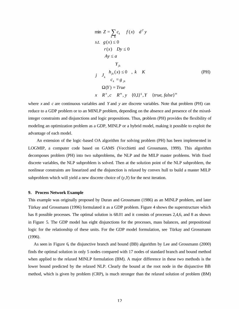
9. Process Network Example

This example was originally proposed by Duran and Grossmann (1986) as an MINLP problem, and later

Türkay and Grossmann (1996) formulated it as a GDP problem. Figure 4 shows the superstructure which

has 8 possible processes. The optimal solution is 68.01 and it consists of processes 2,4,6, and 8 as shown

in Figure 5. The GDP model has eight disjunctions for the processes, mass balances, and prepositional

logic for the relationship of these units. For the GDP model formulation, see Türkay and Grossmann

(1996).

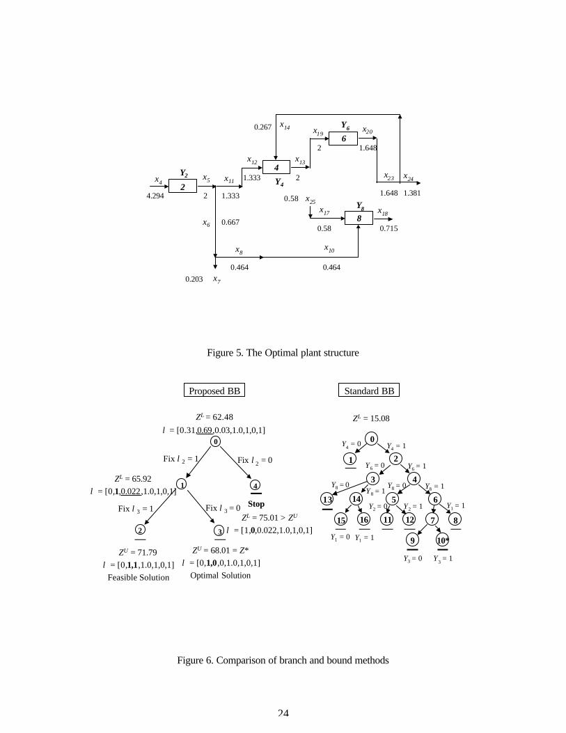
As seen in Figure 6, the disjunctive branch and bound (BB) algorithm by Lee and Grossmann (2000)

finds the optimal solution in only 5 nodes compared with 17 nodes of standard branch and bound method

when applied to the relaxed MINLP formulation (BM). A major difference in these two methods is the

lower bound predicted by the relaxed NLP. Clearly the bound at the root node in the disjunctive BB

method, which is given by problem (CRP), is much stronger than the relaxed solution of problem (BM)

13

(62.48 vs. 15.08). This shows that the logic -based formulation (GDP) yields a tight relaxation that can be

exploited by a disjunctive branch and bound method. On the other hand it is clear that there exists a trade -

off between problems (BM) and (CRP) in terms of problem size and tightness of the lower bound. As in

this example the tight lower bound of (CRP) helped to reduce the number of nodes in the branch and

bound tree, although (BM) is smaller in size and likely to be solved faster.

10. Global Optimization Algorithm

In the previous sections of the paper we have assumed convexity in the nonlinear functions. However, in

many applications nonlinearites give rise to nonconvex functions. Nonlinear programs which involve

nonconvex functions may yield local solutions, not guaranteeing the global optimality. Global

optimization of nonconvex programs has received increased attention due to the practical importance of

solving nonlinear optimization problems. Most of the deterministic global optimization algorithms are

based on spatial branch and bound algorithm (Horst and Tuy, 1996). The spatial branch and bound

method divides the feasible region of continuous variables and compares lower bound and upper bound

for fathoming each subregion. The subregion that contains the optimal solution is found by eliminating

subregions that are proved not to contain the optimal solution.

For nonconvex NLP problems, Quesada and Grossmann (1995) proposed a spatial branch and bound

algorithm for concave separable, linear fractional and bilinear programs using of linear and nonlinear

underestimating functions (McCormick, 1976). For nonconvex MINLP, Ryoo and Sahinidis (1995) and

later Tawarmalani and Sahinidis (2000a) have developed BARON, which branches on the continuous and

discrete variables with bounds reduction method. Adjiman et al. (1997; 2000) proposed the SMIN-αBB

and GMIN-αBB algorithms for twice-differentiable nonconvex MINLPs. By using a valid convex

underestimation of general functions as well as for special functions, Adjiman et al. (1996) developed the

αBB method which branches on both the continuous and discrete variables according to specific options.

The branch-and-contract method (Zamora and Grossmann, 1999) has bilinear, linear fractional, and

concave separable functions in the continuous variables and binary variables, uses bound contraction and

applies the outer-approximation (OA) algorithm at each node of the tree. Kesavan and Barton (2000)

developed a generalized branch-and-cut (GBC) algorithm, and showed that their earlier decomposition

algorithm (Kesavan and Barton, 1999) is a specific instance of the GBC algorithm with a set of heuristics.

Also, Smith and Pantelides (1997) proposed a reformulation method combined with a spatial branch and

bound algorithm for nonconvex MINLP and NLP, which is implemented in the gPROMS modeling

system.

14

11. Nonconvex GDP

We briefly describe a global optimization algorithm proposed by Lee and Grossmann (2001) for the case

when the problem (GDP) involves bilinear, linear fractional and concave separable functions. First, these

nonconvex functions of continuous variables are relaxed by replacing them with underestimating convex

functions (McCormick, 1976; Quesada and Grossmann, 1995). Next, the convex hull of each nonlinear

disjunction is constructed to build a convex NLP problem (CRP). Figure 7 shows the proposed global

optimization procedure. At the first step, an upper bound is obtained by solving the nonconvex MINLP

reformulation (BM) with the OA algorithm. This upper bound is then used for the bound contraction (step

2). The feasible region of continuous variables is contracted with an optimization subproblem that

incorporates the valid underestimators and the upper bound value and that minimizes or maximizes each

variable in turn. The tightened convex GDP problem is then solved in the first level of a two-level branch

and bound algorithm, in which a discrete branch and bound search (see Section 6) is performed on the

disjunctions to predict lower bounds. In the second level, a spatial branch and bound method is used to

solve nonconvex NLP problems for updating the upper bound. The proposed algorithm exploits the

convex hull relaxation for the discrete search, and the fact that the spatial branch and bound is restricted

to fixed discrete variables in order to predict tight lower bounds.

We present an illustrative nonconvex GDP example which was originally proposed as a nonconvex

MINLP by Kocis and Grossmann (1989) for optimizing a small superstructure consisting of two reactors.

Lee and Grossmann (2001) reformulated this problem as the following nonconvex GDP problem:

pcxv

cvp

xvY

cvp

xvY

tspxcZ

,0;200 ;100

(5)

5.50.6

)]4.0exp(1[8.010

5.70.7

)]5.0exp(1[9.010

..5min

21

≤≤≤≤≤

==

−−=∨

==

−−=

++=

The optimal solution is 99.2 with Y* = (true, false), x* = 13.4 and v* = 3.5. Problem (5) has

nonconvex constraints in the disjunction. The global optimization algorithm by Lee and Grossmann

(2001) is applied to problem (5) and its solution results are shown in Table 1. In step 1, a nonconvex

MINLP reformulation (BM) is solved with the OA method. An initial upper bound of 99.2 is obtained

after 3 major iterations. To derive the convex relaxation we first substitute [1-exp(-0.5v)] in the first term

with the continuous variable α, resulting in bilinear terms. The nonlinear equality α = [1-exp(-0.5v)] is

replaced by two nonlinear inequalities.

15

α

αα

α

αα

α

,,0;200 ;100

(6)

5.50.6

)]4.0exp(1[)]4.0exp(1[

8.010

5.70.7

)]5.0exp(1[)]5.0exp(1[

9.010

..5min

21

pcxv

cvp

vv

xY

cvp

vv

xY

tspxcZ

≤≤≤≤≤

==

−−≥−−≤

=

∨

==

−−≥−−≤

=

++=

The bilinear term αx is replaced by linear under and overestimators (McCormick, 1976). In the first

term of the disjunction, the inequality α ≤ [1-exp(-0.5v)] is convex while the inequality α ≥ [1-exp(-

0.5v)] is concave. We underestimate the concave term by a secant line which matches the concave term at

the lower and upper bound of v. The convex underestimating problem of (6) is then as follows:

α

αααα

αααα

ααα

ααα

ααα

αααα

αααα

ααα

ααα

ααα

,,0;200 ;100

(7)

5.50.6

)(

)]4.0exp(1[8.0/10

8.0/10

8.0/10

8.0/10

5.70.7

)(

)]5.0exp(1[9.0/10

9.0/10

9.0/10

9.0/10

..5min

222

22

22

22

22

2

111

11

11

11

11

1

pcxv

cvp

vvvv

vxxx

xxx

xxx

xxx

Y

cvp

vvvv

vxxx

xxx

xxx

xxx

Y

tspxcZ

LU

LULL

ULUL

LULU

LLLL

UUUU

LU

LULL

ULUL

LULU

LLLL

UUUU

≤≤≤≤≤

==

−−

−+≥

−−≤−+≤

−+≤

−+≥

−+≥

∨

==

−−

−+≥

−−≤−+≤

−+≤

−+≥

−+≥

++=

where ).4.0exp(1),4.0exp(1),5.0exp(1),5.0exp(1 2211UULLUULL vvvv −−=−−=−−=−−= αααα

The convex hull relaxation of problem (7) results in problem (CRP). In step 1, we solve the bound

contraction problem of the continuous variable x and v. Initially, the bounds are 0 ≤ x ≤ 20 and 0 ≤ v ≤ 10.

After solving 4 NLPs, the new bounds are 11.1 ≤ x ≤ 18.7 and 1.6 ≤ v ≤ 5.1. With the new bounds, the

discrete branch and bound is performed in step 3. Figure 8 shows the two-level branch and bound tree.

The first lower bound at the root node is 97.5. We relax λ in problem (CRP) as continuous variables

between 0 and 1. λj corresponds to the Boolean variable Y j in problem (GDP) and λ j = 1 in the solution

16

means Y j = true. Solving problem (CRP) yields a discrete feasible solution of λ = (1,0). For convenience,

we denote this value of λ as YL. This integer value is fixed as YF = (1,0) and the upper bound (99.2) is

given to the spatial branch and bound step (node S1 in Figure 8). In step 4, the branching variables are x

and v. The variable with the largest difference in the variable bounds is selected first. The branching

variable and its branching point are shown on each node. At node S1, x is selected first and the branching

point is the middle point of the variable bounds. At node S3, the objective value 99.3 is higher than the

upper bound, so it is fathomed. Node S4 is infeasible and node S5 yields the optimal solu tion. 5 NLPs are

solved with a relative tolerance of 0.1 % and the optimality of the upper bound 99.2 is verified for fixed

YF = (1,0). A logic cut is added to node 1 of step 2 and problem (CRP) is resolved since the gap between

upper and lower bounds is not closed yet at the node 1. Node 2 yields a solution YL = (0.5,0.5) and ZL =

101.6, and hence it is fathomed by the upper bound and the search is finished.

12. Computational results

A number of GDP problems have been solved by Lee and Grossmann (2000, 2001) and their numerical

results are shown in Table 2. These problems were solved with GAMS on a Pentium III PC. The first

column and the second column show the problem number and type. The third column shows the number

of continuous variables, the fourth column shows the number of Boolean variables, and the fifth column

shows the number of constraints, respectively. Problems 1-3 are convex GDP problems and were solved

with the disjunctive branch and bound method described in Section 5. Problems 4-7 are nonconvex GDPs

and they were solved with the two-level branch and bound algorithm. In all cases, the optimal solution is

found in reasonable CPU time as shown in the last column.

13. Conclusion

In this paper, we have presented some of the recent advances in the discrete/continuous optimization

models and solution algorithms. Algebraic models such as MILP and MINLP have been widely used in

operations research and engineering. An emerging approach relies on logic -based models which involve

logic constraints and disjunctions. The strategy for the relaxation of disjunctions and its properties have

been used to develop a disjunctive branch and bound algorithm for GDP problems. Also, the

reformulation to MINLP procedure has been presented, as well as a Cutting Plane method for tightening

the lower bound in the corresponding Big-M formulation. Global optimization algorithms of nonconvex

MINLP/GDP have been also briefly discussed and illustrated with a small example. It is hoped that this

review has shown that the logic -based approach to mathematical programming has made substantial

progress and offers significant promise in the future.

17

Acknowledgments

The authors would like to acknowledge financial support from the NSF Grant CTS-9710303 and from the

Center for Advanced Process Decision-making at Carnegie Mellon University.

References

Adjiman C.S., I.P. Androulakis, C.D. Maranas and C.A. Floudas, A Global Optimization Method, αBB, for Process Design. Computers and Chem. Engng., 20, Suppl., S419-S424, 1996.

Adjiman C.S., I.P. Androulakis and C.A. Floudas, Global Optimization of MINLP Problems in Process Synthesis and Design. Computers and Chem. Engng., 21, Suppl., S445-S450, 1997.

Adjiman C.S., I.P. Androulakis and C.A. Floudas, Global Optimization of Mixed-Integer Nonlinear Problems. AIChE Journal, 46(9), 1769-1797, 2000.

Balas E., An Additive Algorithm for Solving Linear Programs with Zero-One Variables. Operations Research, 13, 517-546, 1965.

Balas E., Disjunctive Programming. Annals of Discrete Mathematics, 5, 3-51, 1979. Balas E., Disjunctive Programming and a Hierarchy of Relaxations for Discrete Optimization Problems.

SIAM J. Alg. Disc. Meth. 6. 466-486, 1985. Balas E., S. Ceria and G. Cornuejols, A Lift-and-Project Cutting Plane Algorithm for Mixed 0-1

Programs. Mathematical Programming, 58, 295-324, 1993. Beaumont N., An Algorithm for Disjunctive Programs. European Journal of Operations Research, 48,

362-371, 1991. Benders J.F., Partitioning Procedures for Solving Mixed Variables Programming Problems. Numerische

Mathematik , 4, 238-252, 1962. Borchers B. and J.E. Mitchell, An Improved Branch and Bound Algorithm for Mixed Integer Nonlinear

Programming. Computers and Operations Research, 21, 359-367, 1994. Ceria S. and J. Soares, Convex Programming for Disjunctive Optimization, Mathematical Programming,

86(3), 595-614, 1999. Crowder H.P., E.L. Johnson and M.W. Padberg, Solving Large-Scale Zero-One Linear Programming

Problems. Operations Research, 31, 803-834, 1983. Dakin R.J., A Tree Search Algorithm for Mixed Integer Programming Problems. Computer Journal, 8,

250-255, 1965. Duran M.A. and I.E. Grossmann, An Outer-Approximation Algorithm for a Class of Mixed-Integer

Nonlinear Programs. Mathematical Programming, 36, 307-339, 1986. Fletcher R. and S. Leyffer, Solving Mixed Nonlinear Programs by Outer Approximation. Mathematical

Programming, 66(3), 327-349, 1994. Geoffrion A.M., Generalized Benders Decomposition. Journal of Optimization Theory and Application,

10(4), 237-260, 1972. Gomory R.E., Outline of an Algorithm for Integer Solutions to Linear Programs. Bulletin of the American

Mathematics Society, 64, 275-278, 1958. Grossmann I.E., Review of Nonlinear Mixed-Integer and Disjunctive Programming Techniques for

Process Systems Engineering. submitted to Journal of Optimization and Engineering, 2002. Grossmann I.E., J.P. Caballero and H. Yeomans, Mathematical Programming Approaches to the

Synthesis of Chemical Process Systems. Korean Journal of Chemical Engineering, 16(4), 407-426, 1999.

Gupta O.K. and V. Ravindran, Branch and Bound Experiments in Convex Nonlinear Integer Programming. Management Science, 31(12), 1533-1546, 1985.

Hentenryck P.V., Constraint Satisfaction in Logic Programming, MIT Press, Cambridge, MA 1989. Hiriart-Urruty J. and C. Lemaréchal, Convex Analysis and Minimization Algorithms, Springer-Verlag,

18

Berlin, New York, 1993. Hooker J.N., Logic-Based Methods for Optimization, John Wiley & Sons, 1999. Hooker J.N. and M.A. Osorio, Mixed logical/linear programming. Discrete Applied Mathematics, 96-97

(1-3). 395-442, 1999. Horst R. and H. Tuy, Global Optimization: Deterministic Approaches, 3rd ed., Springer-Verlag, Berlin,

1996. Johnson E.L., G.L. Nemhauser and M.W.P. Savelsbergh, Progress in Linear Programming Based Branch-

and-Bound Algorithms: An Exposition, INFORMS Journal on Computing, 12, 2000. Kallrath J., Mixed Integer Optimization in the Chemical Process Industry: Experience, Potential and

Future. Trans. I. Chem. E., 78, Part A, 809-822, 2000. Kesavan P. and P.I. Barton, Decomposition algorithms for nonconvex mixed-integer nonlinear programs.

American Institute of Chemical Engineering Symposium Series, (in press) 1999. Kesavan P. and P.I. Barton, Generalized branch-and-cut framework for mixed-integer nonlinear

optimization problems. Computers Chem. Engng., 24, 1361-1366, 2000. Kelley Jr. J.E., The Cutting-Plane Method for Solving Convex Programs. Journal of SIAM , 8, 703, 1960. Kocis G.R. and I.E. Grossmann, Relaxation Strategy for the Structural Optimization of Process

Flowsheets. Ind. Eng. Chem. Res. 26, 1869, 1987. Kocis G.R. and I.E. Grossmann, A Modelling and Decomposition Strategy for the MINLP Optimization

of Process Flowsheets. Computers and Chem. Engng., 13(7), 797-819, 1989. Land A.H. and A.G. Doig, An Automatic Method for Solving Discrete Programming Problems.

Econometrica, 28, 497-520,1960. Lee S. and I.E. Grossmann, New Algorithms for Nonlinear Generalized Disjunctive Programming.

Computers Chem. Engng., 24, 2125-2141, 2000. Lee S. and I.E. Grossmann, A Global Optimization Algorithm for Nonconvex Generalized Disjunctive

Programming and Applications to Process Systems. Computers Chem. Engng., 25, 1675-1697, 2001. Leyffer S., Integrating SQP and branch-and-bound for Mixed Integer Nonlinear Programming.

Computational Optimization and Applications 18, 295-309, 2001. Lovász L. and A. Schrijver, Cones of matrices and set-functions and 0-1 optimization. SIAM Journal on

Optimization, 12, 166-190, 1991. McCormick G.P., Computability of Global Solutions to Factorable Nonconvex Programs: Part I – Convex

Underestimating Problems. Mathematical Programming, 10, 147-175, 1976. Nemhauser G.L. and L.A. Wolsey, Integer and Combinatorial Optimization, Wiley-Interscience, New

York, 1988. Quesada I. and I.E. Grossmann, An LP/NLP Based Branch and Bound Algorithm for Convex MINLP

Optimization Problems. Computers Chem. Engng., 16(10/11), 937-947, 1992. Quesada I. and I.E. Grossmann, A Global Optimization Algorithm for Linear Fractional and Bilinear

Programs. Journal of Global Optimization, 6(1), 39-76, 1995. Raman R. and I.E. Grossmann, Relation Between MILP Modelling and Logical Inference for Chemical

Process Synthesis. Computers Chem. Engng., 15(2), 73-84, 1991. Raman R. and I.E. Grossmann, Modelling and Computational Techniques for Logic Based Integer

Programming. Computers Chem. Engng., 18(7), 563-578, 1994. Ryoo H.S. and N.V. Sahinidis, Global Optimization of Nonconvex NLPs and MINLPs with Applications

in Process Design. Computers and Chem. Engng., 19(5), 551-566, 1995. Sherali H.D. and W.P. Adams, A Hierarchy of Relaxations Between the Continuous and Convex Hull

Representations for Zero-One Programming Problems. SIAM Journal on Discrete Mathematics, 3(3), 411-430, 1990.

Smith E.M.B. and C.C. Pantelides, Global optimization of nonconvex NLPs and MINLPs with applications in process design. Computers Chem. Engng., 21(1001), S791-S796, 1997.

Stubbs R. and S. Mehrotra, A Branch-and-Cut Method for 0-1 Mixed Convex Programming. Mathematical Programming, 86(3), 515-532, 1999.

Türkay M. and I.E. Grossmann, Logic-based MINLP Algorithms for the Optimal Synthesis of Process

19

Networks. Computers Chem. Engng., 20(8), 959-978, 1996. Van Roy T.J. and L.A. Wolsey, Valid Inequalities for Mixed 0-1 Programs. Discrete Applied

Mathematics, 14, 199-213, 1986. Vecchietti A. and I.E. Grossmann, LOGMIP: A Disjunctive 0-1 Nonlinear Optimizer for Process Systems

Models. Computers Chem. Engng., 23, 555-565, 1999. Viswanathan J. and I.E. Grossmann, A Combined Penalty Function and Outer-Approximation Method for

MINLP Optimization. Computers Chem. Engng., 14, 769, 1990. Yuan X, S. Zhang, L. Piboleau and S. Domenech, Une Methode d′optimization Nonlineare en Variables

Mixtes pour la Conception de Porcedes. Rairo Recherche Operationnele, 22, 331, 1988. Westerlund T. and F. Pettersson, An Extended Cutting Plane Method for Solving Convex MINLP

Problems. Computers Chem. Engng., 19, supl., S131-S136, 1995. Williams H.P., Mathematical Building in Mathematical Programming, John Wiley, Chichester, 1985. Zamora J.M. and I.E. Grossmann, A Branch and Bound Algorithm for Problems with Concave

Univariate, Bilinear and Linear Fractional Terms. Journal of Global Optimization, 14(3), 217-249, 1999.

20

List of Tables

Table 1. Numerical results of illustrative example Table 2. Numerical results of GDP problems

Table 1. Numerical results of illustrative example

Step Method

Step 1 Outer

Approximation

Step 2 Bound

Contraction

Step 3 Discrete

Branch and Bound

Step 4 Spatial

Branch and Bound Result

Iter. / Nodes First UB = 99.2

3 Iter. 63.5 % reduction

4 Iter. (NLPs) First LB = 97.5 2 Nodes (NLPs)

1 SBB / UB = 99.2 5 Nodes (NLPs)

Table 2. Numerical results of GDP problems

Problem Number

Problem Type

No. of continuous variables

No. of Boolean variable

No. of constraints

Optimal solution

CPU sec

1 Convex 30 25 105 -8.064 2.86 2 Convex 33 8 67 68.01 1.09 3 Convex 184 41 376 261,883 40.91 4 Nonconvex 51 33 102 264,887 47.1 5 Nonconvex 105 53 271 726,205 163.7 6 Nonconvex 312 59 1231 662,590 521.3 7 Nonconvex 52 16 124 74,710 420.6

21

List of Figures

Figure 1. Feasible set and convex hull of example 1

Figure 2. Feasible set at the first node

Figure 3. Feasible set at the second node

Figure 4. Superstructure for process network example

Figure 5. The optimal plant structure

Figure 6. Comparison of branch and bound methods

Figure 7. Global optimization algorithm for nonconvex GDP

Figure 8. Branch and bound tree for nonconvex GDP example

22

x1

x2

Convex hullS3

S2

S1

Figure 1. Feasible set and convex hull of example 1

First Node : S2 Optimal solution : ZU = 1.172

x1

x2S3

S1

Optimal Solution(3.293,1.707)

Z* = 1.172

S2

Figure 2. Feasible set at the first node

23

Second Node : conv(S1 ∨ S3)Optimal solution : ZL = 3.327

x1

x2

S3

S2

S1

Upper BoundZU = 1.172

Lower BoundZL = 3.327

Figure 3. Feasible set at the second node

1

2

6

7

4

3

5 8

x1

x4

x6

x21

x19

x13

x14

x11

x7

x8

x12

x15

x9

x16 x17

x25

x18

x10

x20

x23x22 x24x5

x3x2

Y1

Y8

Y7

Y6

Y4

Y5

Y3

Y2

Figure 4. Superstructure for process network example

24

2

6

4

8

x4

x6

x19

x13

x14

x11

x7

x8

x12

x17

x25x18

x20

x23 x24x5

Y8

Y6

Y4

Y2

x10

4.294 2

0.667

1.333

1.6482

0.267

21.333

0.4640.203

1.648 1.381

0.715

0.464

0.58

0.58

Figure 5. The Optimal plant structure

ZL = 62.48λ = [0.31,0.69,0.03,1.0,1,0,1]

ZU = 68.01 = Z*λ = [0,1,0,0,1.0,1,0,1]

Optimal Solution

ZU = 71.79λ = [0,1,1,1.0,1,0,1]

Feasible Solution

ZL = 75.01 > ZU

λ = [1,0,0.022,1.0,1,0,1]

ZL = 65.92λ = [0,1,0.022,1.0,1,0,1]

0

32

41

Fix λ2 = 1

Fix λ3 = 1 Fix λ3 = 0

Fix λ2 = 0

Stop

0

ZL = 15.08

Standard BB

1 2

43

1413 5 6

812111615 7

10*9

Y4 = 0 Y4 = 1

Proposed BB

Y6 = 0 Y6 = 1

Y8 = 0Y8 = 1

Y1 = 0 Y1 = 1

Y8 = 0 Y8 = 1

Y2 = 0 Y2 = 1 Y1 = 1

Y3 = 0 Y3 = 1

Figure 6. Comparison of branch and bound methods

25

Nonconvex MINLP

Bound Contraction

New Bound

BB with Y ’ s Update Z L

Spatial BB

When all Y ’ s are fixed

Update Z U

Stop when Z L ≥ Z U

Add Cut

Step1

Fixed Y ’ s

Step3

Step2

Step4

Z U

OA (Viswanathan and Grossmann, 1990)

( Zamora and Grossmann, 1999)

( Lee and Grossmann, 2000)

( Quesada and Grossmann, 1995)

Figure 7. Global optimization algorithm for nonconvex GDP

ZL = 97.5YL = (1,0)

Spatial BB

cut

YF = (1,0)1S1

2

infeasible

Discrete BB

fathomed

ZL = 101.6YL = (0.5,0.5)

x ≤ 13.6

Z = 97.5

13.6 ≤ x

Z = 99.3

fathomed

S2 S3

S4 S5

v ≤ 3.36

Z = 98.3

3.36 ≤ v

Z = 99.2

Figure 8. Branch and bound tree for nonconvex GDP example