Loewner Equation Derivative
14
the loewner equation and the derivative of its solution Carl Ringqvist February 26, 2015 Master’s Thesis presentation, KTH & SU
description
Example of latex template. Carl Ringqvist
Transcript of Loewner Equation Derivative

the loewner equation and the derivative ofits solution
Carl RingqvistFebruary 26, 2015
Master’s Thesis presentation, KTH & SU

Introduction
Charles Loewner and the introduction of the Loewner Equation.
1

Illustrations
Some examples of driving functions Ut
Source: ”Spacefilling Curves and Phases of the Loewner Equation”, J.Lind, S.Rohde
2

Illustrations
And the sets they generate
Figure: van Koch curve, the half-Sierpinski gasket, and the Hilbertspace-filling curve
Source: ”Spacefilling Curves and Phases of the Loewner Equation”, J.Lind, S.Rohde 3

the SLE-curve
Let Ut =√κBt, where κ ∈ R and Bt is a standard Brownian motion.
Then, with probability one, the set Ht is generated by a curve, i.eHt = H\γ(0, t] for some continuous curve γ. This γ is called anSLE-curve. Two interesting facts about the SLE-curve:
∙ The curve spirals at every point∙ The trace is extremely sensitive to the value of κ. In fact∙ For 0 ≤ κ ≤ 4 the trace γ is simple with probability one.∙ For 4 ≤ κ < 8 the trace γ intersects itself and every point is containedin a loop but the curve is not space-filling (with probability 1).
∙ For κ ≥ 8 the trace γ is space-filling (with probability 1).
4

Illustrations
κ = 2, yielding a simple trace:
Source: http://iopscience.iop.org
5

Illustrations
κ = 6, yielding a non-simple trace:
Source: http://iopscience.iop.org
6

Discrete Gaussian free fields
Rougher grid left, finer grid right
Source: ”Finding SLE paths in the Gaussian free field ”, S.L. Watson
7
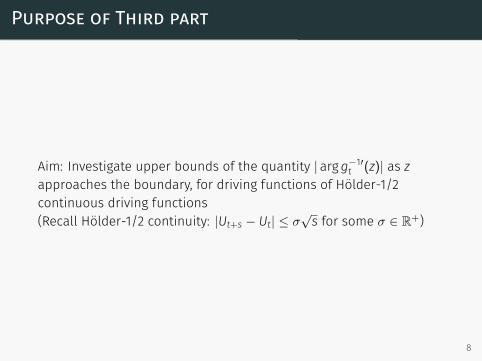
Purpose of Third part
Aim: Investigate upper bounds of the quantity | argg−1′t (z)| as zapproaches the boundary, for driving functions of Hölder-1/2continuous driving functions(Recall Hölder-1/2 continuity: |Ut+s − Ut| ≤ σ
√s for some σ ∈ R+)
8
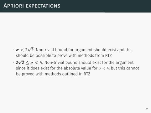
Apriori expectations
∙ σ < 2√2: Nontrivial bound for argument should exist and this
should be possible to prove with methods from RTZ∙ 2
√2 ≤ σ < 4. Non-trivial bound should exist for the argument
since it does exist for the absolute value for σ < 4; but this cannotbe proved with methods outlined in RTZ
9

An illuminating example
In the article ”Collisions and spirals of Loewner traces” by Lind, Marshall andRohde, the Loewner trace and conformal map of the driving functionUt = σ
√1− t, 0 < σ < 4 are calculated. In fact here the following is stated:
Given 0 < σ < 4, set θ := − sin−1(σ/4), β = 2ieiθ , and set
k(z) = (z−β)(z−β)e2iθ
(σ−β)(σ−β)e2iθ
gt(z) = (1− t)1/2k−1((1− t)− cos θeiθk(z))
Then k is a conformal map of H onto C\G where G := {eteiθ; t ≥ 0}, is a
logarithmic spiral in C beginning at 1 and tending to∞, and where gtsatisfies the Loewner equation
gt =2
gt − σ√1− t
g0 ≡ z
The trace γ = k−1({e−teiθ ; t > 0}) is a curve in H beginning at σ ∈ Rspiraling around β ∈ H 10

11

Results
∙ σ <√2: A non-trivial bound is obtained in line with expectation.
∙√2 ≤ σ < 2
√2: We show the methods of RTZ are insufficient for
obtaining a non-trivial bound in this interval. However, we stillsuspect such a nontrivial bound to exist
∙ 2√2 ≤ σ < 4: We have shown no non-trivial bound can exist in
this interval
12

Questions?
13


![[-2em]Conformally Invariant Processes and the Schramm–Loewner ...](https://static.fdocuments.us/doc/165x107/5870bfda1a28ab87318b5a40/-2emconformally-invariant-processes-and-the-schrammloewner-.jpg)