LOCATIONS ON A LINE AND GENERALIZATION TO THE DYNAMIC P-MEDIANS

A THESIS SUBMITED TO THE GRADUATE SCHOOL OF NATURAL AND APPLIED SCIENCES

OF MIDDLE EAST TECHNICAL UNIVERSITY

BY

HÜSEYİN GÜDEN

IN PARTIAL FULFILLMENT OF THE REQUIREMENTS FOR

THE DEGREE OF DOCTOR OF PHILOSOPHY IN

INDUSTRIAL ENGINEERING

SEPTEMBER 2012

Approval of the thesis:

LOCATIONS ON A LINE AND GENERALIZATION TO THE DYNAMIC

P-MEDIANS

submitted by HÜSEYİN GÜDEN in partial fulfillment of the requirements for the degree of Doctor of Philosophy in Industrial Engineering Department, Middle

East Technical University by, Prof. Dr. Canan Özgen Dean, Graduate School of Natural and Applied Science

Prof. Dr. Sinan Kayalıgil Head of Department, Industrial Engineering

Assoc. Prof. Dr. Haldun Süral Supervisor, Industrial Engineering Dept., METU Examining Committee Members:

Prof. Dr. Ömer Kırca Industrial Engineering Dept., METU Assoc. Prof. Dr. Haldun Süral Industrial Engineering Dept., METU Assoc. Prof. Dr. Bahar Yetiş Kara Industrial Engineering Dept., Bilkent Univ. Assoc. Prof. Dr. Hande Yaman Industrial Engineering Dept., Bilkent Univ. Assist. Prof. Dr. Sinan Gürel Industrial Engineering Dept., METU

Date :

iii

I hereby declare that all information in this document has been obtained and

presented in accordance with academic rules and ethical conduct. I also

declare that, as required by these rules and conduct, I have fully cited and

referenced all material and results that are not original to this work.

Name, Last name : Hüseyin, GÜDEN

Signature :

iv

ABSTRACT

LOCATIONS ON A LINE AND GENERALIZATION TO THE DYNAMIC

P-MEDIANS

Güden, Hüseyin

Ph.D., Department of Industrial Engineering

Supervisor: Assoc. Prof. Dr. Haldun Süral

September 2012, 173 pages

This study deals with four location problems. The first problem is a brand new

location problem on a line and considers the location decisions for depots and

quarries in a highway construction project. We develop optimal solution properties

of the problem. Using these properties, a dynamic programming algorithm is

proposed. The second problem is also a brand new dynamic location problem on a

line and locates concrete batching mobile and immobile facilities for a railroad

construction project. We develop two mixed integer models to solve the problem.

For solving large size problems, we propose a heuristic. Performances of models

and the heuristic are tested on randomly generated instances plus a case study data

and results are presented. The third problem is a generalization of the second

problem to network locations. It is a dynamic version of the well known p-median

problem and incorporates mobile facilities. The problem is to locate predetermined

number of mobile and immobile facilities over a planning horizon such that sum of

facility movement and allocation costs is minimized. Three constructive heuristics

and a branch-and-price algorithm are proposed. Performances of these solution

v

procedures are tested on randomly generated instances and results are presented. In

the fourth problem we consider a special case of the third problem, allowing only

conventional facilities. The algorithm for the third problem is improved so that

generating columns and solving a mixed integer model are used repetitively.

Performance of the algorithm is tested on randomly generated instances and results

are presented.

Keywords: Dynamic location, p-median, mobile facilities, location on a line,

branch and price.

vi

ÖZ

HAT ÜZERİNDE YER SEÇİMİ VE DİNAMİK P-MEDYANA

GENELLEŞTİRİLMESİ

Güden, Hüseyin

Doktora, Endüstri Mühendisliği Bölümü

Tez Yöneticisi: Doç. Dr. Haldun Süral

Eylül 2012, 173 sayfa

Bu çalışmada dört yer seçimi problemi işlenmiştir. İlki tamamen yeni, bir hat

üzerinde yer seçimi problemidir ve bir otoban yapımı projesinin depo ve ocak

yerlerinin seçilmesi kararlarını ele alır. Problemin en iyi çözümünün özellikleri

belirlenmiştir. Bu özellikler kullanılarak bir dinamik programlama algoritması

önerilmiştir. İkinci problem de tamamen yeni; bir dinamik, kapasiteli, hat üzerinde

yer seçimi problemidir ve bir demiryolu yapımı projesinin seyyar ve sabit beton

santrallerinin yerlerini belirler. Problemin çözümü için iki karışık tamsayılı

matematiksel model geliştirilmiştir. Büyük boyutlu problemleri çözmek için

problem boyutunu küçülten bir sezgisel önerilmiştir. Modellerin ve sezgiselin

performansları rasgele oluşturulan problemler artı bir vaka çalışması verileri

üzerinde test edilmiş ve sonuçları sunulmuştur. Üçüncü problem ikincinin (genel)

serim üzerindeki yer seçimi problemlerine genelleştirilmisidir. Bu problem çok

bilinen p-medyan probleminin dinamik halidir ve seyyar tesisler içerir. Problem bir

planlama ufkunda belli sayıdaki seyyar ve sabit tesisleri, tesis taşıma ve talepleri

zamanla değişen müşterilerin tesislere atanma maliyetlerinin toplamını en

vii

küçükleyecek şekilde yerleştirmektir. Üç kurucu sezgisel ve bir dallandır-ve-

fiyatlandır algoritması önerilmiştir. Bu çözüm yöntemlerinin performansları rasgele

oluşturulan problemler üzerinde test edilmiş ve sonuçları sunulmuştur. Dördüncü

problemde üçüncü problemin özel bir hali, sadece sabit tesislerin olduğu durum

işlenmiştir. Üçüncü problem için geliştirilen algoritma, kolonların oluşturulmasının

ve karışık tamsayılı model çözümünün tekrarlı kullanılmasıyla iyileştirilmiştir. Bu

yeni algoritmanın performansı rasgele oluşturulan problemler üzerinde test edilmiş

ve sonuçları sunulmuştur.

Anahtar Kelimeler: Dinamik yer seçimi, p-medyan, seyyar tesisler, hat üzerinde

yerleşim, dallandır ve fiyatlandır

viii

TABLE OF CONTENTS

ABSTRACT ………………………….......…….….………………...........…….... iv

ÖZ …………………..……………………………….............................................. vi

TABLE OF CONTENTS ………………………………...................................... viii

LIST OF TABLES ………………......................………………............……....… xi

LIST OF FIGURES ……………………….............................……................….. xiii

LIST OF ABBREVIATIONS ............................................................................... xiv

CHAPTERS

1. INTRODUCTION ........................................................................................ 1

2. THE DEPOT-QUARRY LOCATION PROBLEM IN ROAD

CONSTRUCTION ....................................................................................... 5

2.1. Problem Definition .................................................................................. 5

2.2. Literature Review .................................................................................... 8

2.3. Fixed Charge Network Flow Problem Formulation of the DQLP......... 11

2.4. Properties of the Optimal Solution of the DQLP ................................. 13

2.5. An Ideal Formulation for the DQLP and a DP Algorithm ................... 18

2.6. Relations between the DQLP and the ULSPB over the Network ....... 20

2.7. The Complexity of the Algorithms for the DQLP and the ULSPB ..... 24

3. A DYNAMIC LOCATION PROBLEM IN RAILROAD

CONSTRUCTION ..................................................................................... 29

3.1. Problem Definition ................................................................................ 29

3.2. Literature Review .................................................................................. 33

3.3. Two MIP formulations for the Problem ................................................ 38

3.4. A Preprocessing Heuristic to Reduce the Number of Candidate Sites...43

3.5. Computational Results ......................................................................... 45

3.5.1. Case Study ...................................................................................... 45

3.5.2. Performance of the Preprocessing Heuristic ................................... 51

A. Tests on the Case Study Problem .................................................... 51

B. Tests on the Randomly Generated Test Instances .......................... 52

ix

4. THE DYNAMIC P-MEDIAN PROBLEM WITH MOBILE

FACILITIES................................................................................................ 54

4.1. Introduction ........................................................................................... 54

4.2. Literature Review .................................................................................. 55

4.2.1. Literature Review on the p-Median Problem .................................. 55

4.2.2. Literature Review on the Dynamic p-Median Problem .................. 64

4.3.Mathematical Formulation of the Dynamic p-Median Problem with

Mobile Facilities: Dynamic Radius Formulation (DRF) ....................... 66

4.4. Solution Methods .................................................................................. 74

4.4.1. Heuristics ........................................................................................ 74

4.4.2. Branch and Price Algorithm (BnP) ................................................. 78

4.5. Computational Results .......................................................................... 84

4.5.1. Validation of DBnP ......................................................................... 87

4.5.2. Experiments on the First Problem Class Involving Only Mobile

Facilities .......................................................................................... 89

A. Testing Performances of Heuristics and Parameter Setting ........... 89

B. Testing performance of DBnP ........................................................ 91

4.5.3. Experiments on the Second Problem Class Involving Mobile and

Immobile Facilities ......................................................................... 93

A. Testing Performances of Heuristics and Parameter Setting .......... 93

B. Testing performance of DBnP ........................................................ 95

5. THE DYNAMIC P-MEDIAN PROBLEM .............................................. 97

5.1. Introduction .......................................................................................... 97

5.2. Mathematical Formulation of the Dynamic p-Median Problem ........... 99

5.3. An Iterative MIP based Column Generation Algorithm for the Dynamic

p-Median Problem ................................................................................ 100

5.4. Computational Results ........................................................................ 104

5.4.1. Performances of the Heuristics and DBnP in Chapter 4 ............... 105

A. Testing Performances of Heuristics and Parameter Setting ......... 105

B. Testing performance of DBnP ...................................................... 107

5.4.2. Performance of IMCA .................................................................. 109

A. Validation of IMCA ....................................................................... 109

x

B. Testing performance of IMCA ...................................................... 110

6. CONCLUSION ......................................................................................... 112

REFERENCES ..................................................................................................... 117

APPENDICES

A. SETTINGS FOR THE RANDOMLY GENERATED TEST PROBLEM

INSTANCES AND THE PROCEDURE TO GENERATE THESE

INSTANCES ............................................................................................ 124

B. DETAILS AND FLOW CHART OF THE BRANCH-AND-PRICE

ALGORITHM DEVELOPED .................................................................. 126

C. DETAILED RESULTS OF COMPUTATIONS IN CHAPTER 4 ......... 130

D. DETAILED RESULTS OF COMPUTATIONS IN CHAPTER 5 ......... 154

E. CURRICULUM VITAE .......................................................................... 169

xi

LIST OF TABLES

TABLES

Table 3.1 Number of open facilities, solution values by M2, and deviation of the

solution value by M2 relative to the linear solution to M2 for the case study

problem with varying costs .................................................................................... 47

Table 3.2 Results for a set of facility movement cost values (1,000 TL) .............. 48

Table 3.3 Results for different mobile facility construction costs (1,000 TL) ...... 48

Table 3.4 Results for different immobile facility construction costs (1,000 TL) .. 49

Table 3.5 Results for the p-median problem with mobile facilities (1,000 TL) .... 50

Table 3.6 Deviation of the solution value relative to the best lower bound and

solution time for M2 and M2(R) for the case study problem with varying costs ... 51

Table 3.7 Deviation of the solution value relative to the best lower bound and

solution time for M2 and M2(R) for randomly generated test problems with varying

costs ........................................................................................................................ 53

Table 4.1 Features of present study and the related studies in the literature ......... 66

Table 4.2 Solution times (sec.) for the p-median problem test instances in the first

group ....................................................................................................................... 88

Table 4.3 Average solution times and relative gaps for the heuristics................... 90

Table 4.4 Summary of average results for the first problem class.......................... 92

Table 4.5 Average solution times and relative gaps for the heuristics................... 94

Table 4.6 Summary of average results for the second type problem instances .... 96

Table 5.1 Average solution times and relative gaps for the heuristics ................ 106

Table 5.2 Summary of average results for the instances in the second group and

DBnP .................................................................................................................... 108

Table 5.3 Solution times (sec.) for the test problem instances in the first group . 110

Table 5.4 Summary of average results for the dynamic p-median problem instances

and IMCA ............................................................................................................. 111

xii

Table C.1 Results for the myopic heuristic for the first problem class for the

instances in the subset A of the second group of the test instances ...................... 130

Table C.2 Results for the progressive heuristics for the first problem class for the

instances in the subset A of the second group of the test instances ...................... 134

Table C.3 Results for myopic heuristic starting from the last period and DBnP with

different target values for the first problem class for the instances in the subset A of

the second group of the test instances .................................................................. 136

Table C.4 Results for the first problem class obtained by DBnP ........................ 139

Table C.5 Results for the myopic heuristic for the second problem class for the

instances in the subset A of the second group of the test instances ...................... 142

Table C.6 Results for the progressive heuristics for the second problem class for

the instances in the subset A of the second group of the test instances ................ 146

Table C.7 Results for myopic heuristic starting from the last period and DBnP with

different target values for the second problem class for the instances in the subset A

of the second group of the test instances .............................................................. 148

Table C.8 Results for the second problem class obtained by DBnP ................... 151

Table D.1 Results for the myopic heuristic for the instances in the subset A of the

second group of the test instances ........................................................................ 154

Table D.2 Results for the progressive heuristics for the instances in the subset A of

the second group of the test instances .................................................................. 158

Table D.3 Results for myopic heuristic starting from the last period and DBnP with

different target values for the instances in the subset A of the second group of the

test instances ......................................................................................................... 160

Table D.4 Results for DBnP ................................................................................ 163

Table D.5 Results for IMCA ............................................................................... 166

xiii

LIST OF FIGURES

FIGURES

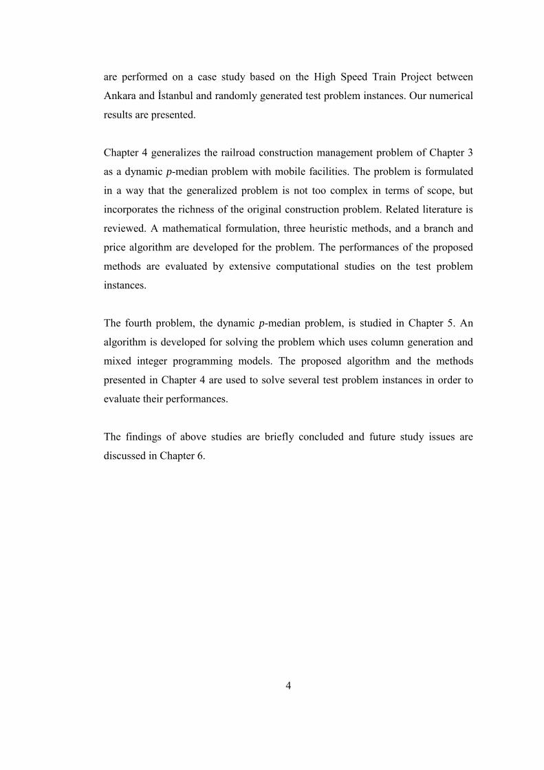
Figure 2.1 An illustration for a road construction Project ....................................... 6

Figure 2.2 G for a DQLP example with n=9 ........................................................ 11

Figure 2.3 Extreme solutions for the DQLP example given in Figure 2.2. ........... 14

Figure 2.4 The SPP network for the DQLP with n=4 ........................................... 19

Figure 2.5 An extreme solution example for an ULSPB instance with 9 periods

where di is the demand in period i, i=1, …,9 .......................................................... 23

Figure 3.1 Art buildings ......................................................................................... 30

Figure 3.2 Tunnel construction process ................................................................. 30

Figure 3.3 Viaduct construction process ............................................................... 31

Figure 3.4 A vertical cross section of a railroad .................................................... 32

Figure 3.5 Railroad, transportation line, resource points, and demand points in a

railroad construction project ................................................................................... 32

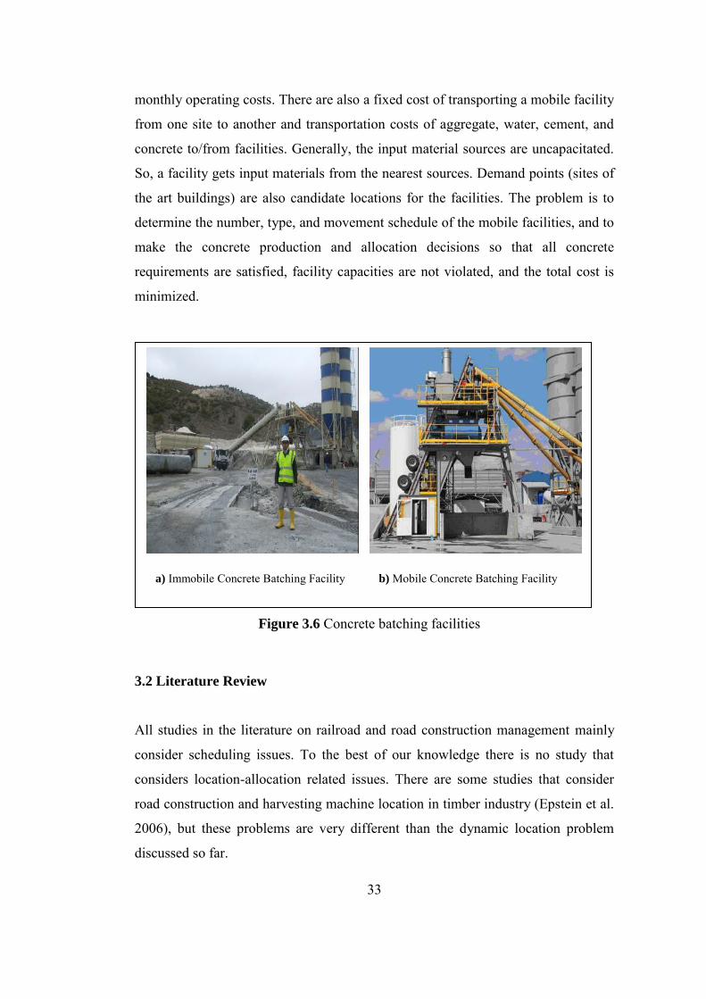
Figure 3.6 Concrete batching facilities .................................................................. 33

Figure 4.1 Illustration of z variables used in Model 6 ........................................... 62

Figure 4.2 Illustration of the myopic heuristic ...................................................... 77

Figure B.1: Flow chart of the DBnP algorithm ................................................... 129

xiv

LIST OF ABBREVIATIONS

BnB : branch and bound

BnC : branch and cut

BnP : branch and price

DBnP : dynamic branch and price

DP : dynamic programming

DPP : dynamic p-median problem

DQLP : depot-quarry location problem

DRF : dynamic radius formulation

FNFP : fixed charge network flow problem

IMCA : Iterative MIP based column generation algorithm

LB : lower bound

LP : linear programming

LPR : linear programming relaxation

MIP : mixed integer programming

MH : myopic heuristic

P1 : progressive heuristic 1

P2 : progressive heuristic 2

SPP : shortest path problem

UB : upper bound

UFLP : uncapacitated facility location problem

ULSPB : uncapacitated lot sizing problem with backlogging

CHAPTER 1

INTRODUCTION

This thesis deals with four rich location problems. They are rich not because we

introduce two of them for the first time and consider extensively the other two

problems, but because they are extended location problems with new or rare

features like having dynamic nature and incorporating mobile facilities. The first

problem is about the location of depots and quarries in a highway construction

project. The second problem is about the location of mobile and immobile concrete

batching facilities for a railroad construction project. Both problems are motivated

by real life applications in construction management. The third problem generalizes

our findings for the second problem to general networks under the p-median

problem settings. The resultant problem is a dynamic version of the p-median

problem with mobile facilities. The fourth problem is a special case of the third

problem where all facilities are assumed to be immobile.

The first problem is a new location problem, called the depot-quarry location

problem. The problem is to locate facilities on a line and occurs in road

construction projects. There are capacitated cut (supply) and fill (demand) points on

the road so that the supply amounts must be cut from the cut points and should be

filled in the fill points. Moreover, there are candidate uncapacitated depot and

quarry sites that can be used to heap or obtain supply if the total cut and fill

amounts are not balanced or a gain is achieved because of shortening transportation

distances, if possible. Besides transportation costs, there are fixed and variable costs

related with depots and quarries. The problem is to determine the depot and quarry

points that will be used and the material flows between cuts, fills, depots, and

quarries such that total cost is minimized, and the material is removed (filled) from 1

2

(to) the cut (fill) points. The problem is tightly related with the uncapacitated lot

sizing problem with backlogging. Similarities and differences between these two

problems, their optimal solution properties, and their solution methods are studied

in detail. We develop two types of mathematical formulations: the fixed charged

network flow problem type and the shortest path problem type. A polynomial time

dynamic programming algorithm is presented for solving the problem.

The second problem is a dynamic, capacitated location problem with mobile and

immobile facilities and it occurs in railroad construction projects. In rail road

construction projects (im)mobile concrete batching facilities are located to build

viaducts and tunnels. These facilities are built on a line over a time horizon. There

are fixed costs of opening and moving facilities. There are also costs of operating

facilities and transportation costs of concrete from facilities to construction sites.

Concrete requirements of sites are obtained from the construction schedule. The

problem is to determine the number, type, and movement schedule of the facilities

and to make the concrete production and allocation decisions so that all concrete

requirements are satisfied, facility capacities are not violated, and the total cost is

minimized. We develop two strong mixed integer models. For solving large size

problems, we propose a heuristic to reduce the problem size and obtain

approximate solutions. We test models and heuristic performances on a case study

problem based on real life data and randomly generated small, medium, and big

size test instances.

The dynamic demands and mobile facilities are two distinctive properties of the

second problem. Being motivated by these properties, in the third problem the

second problem is generalized to the general networks under the p-median problem

settings, called the dynamic p-median problem (DPP) with mobile facilities. There

are dynamic demands over a planning horizon and predetermined numbers of

mobile and immobile facilities in each period. According to some external

considerations the number of facilities may or may not change from period to

period. If the number of facilities for a type decreases in a period compared to the

previous period, then some of these facilities should be abolished in that period. If it

3

increases, then some of new facilities for that type must be opened. If it does not

change, then there will be no opening and no abolishing for that type. Abolishing

and opening cannot be realized simultaneously at a site. During the planning

horizon facility opening, moving, and abolishing may occur several times over the

horizon at a location. There are relocation (moving) costs (fixed or source-and-sink-

location dependent) for mobile facilities and service (allocation) costs for all types.

The problem is to determine (i) the opening or abolishing periods and locations of

the facilities, (ii) movement periods and routes of the mobile facilities, and (iii)

allocation of the demand nodes to open facilities in each period such that total cost

is minimized. Three constructive heuristics and a branch and price algorithm are

proposed. Performances of these solution procedures are tested on randomly

generated instances and their results are presented.

In the fourth problem we consider a special case of the third problem, allowing only

conventional (immobile) facilities. There are dynamic demands over a planning

horizon and a predetermined number of facilities in each period. The branch-and-

price algorithm developed for the third problem is improved so that generating

columns and solving a mixed integer model of a variant of the problem are used

repetitively. Performance of the new modified algorithm is tested on randomly

generated instances and their results are presented.

The remaining chapters are organized as follows. The depot-quarry location

problem is presented in the second chapter. Related literature is also reviewed in

Chapter 2. Different mathematical formulations of the problem and our solution

approach based on a dynamic programming algorithm are presented. The relations

between the depot-quarry location problem and the uncapacitated lot sizing

problem with backlogging are studied in Chapter 2.

Chapter 3 contains the second problem. The problem and the related studies in the

literature are explained in detail. Two mathematical formulations of the problem

and our preprocessing heuristic that reduces the number of candidate sites (also

reduces the problem size and its model size) are presented. Computational studies

4

are performed on a case study based on the High Speed Train Project between

Ankara and İstanbul and randomly generated test problem instances. Our numerical

results are presented.

Chapter 4 generalizes the railroad construction management problem of Chapter 3

as a dynamic p-median problem with mobile facilities. The problem is formulated

in a way that the generalized problem is not too complex in terms of scope, but

incorporates the richness of the original construction problem. Related literature is

reviewed. A mathematical formulation, three heuristic methods, and a branch and

price algorithm are developed for the problem. The performances of the proposed

methods are evaluated by extensive computational studies on the test problem

instances.

The fourth problem, the dynamic p-median problem, is studied in Chapter 5. An

algorithm is developed for solving the problem which uses column generation and

mixed integer programming models. The proposed algorithm and the methods

presented in Chapter 4 are used to solve several test problem instances in order to

evaluate their performances.

The findings of above studies are briefly concluded and future study issues are

discussed in Chapter 6.

5

CHAPTER 2

THE DEPOT-QUARRY LOCATION PROBLEM IN ROAD

CONSTRUCTION

In this chapter, a new location problem, called the Depot-Quarry Location Problem

(DQLP), is introduced. It is a location problem on a line and appears in road

construction projects. Some characteristics of the problem related with demand-

supply relations and capacity limitations are quite different than those of the

traditional location problems.

2.1 Problem Definition

In a road construction project, “smoothing” is needed after the road line and its

altitude are determined. Smoothing basically includes cutting the hills and filling

the holes by using the transported material (earth) from cut (supply) points to fill

(demand) points. If the distance between demand and supply points is long, and/or

the total amounts of supply and demand are not balanced, some additional sites are

needed in order to match demand with supply. Such sites are called depots (or

oversupply case) and quarries (or undersupply case) and they are usually assumed

to be uncapacitated. Note that a depot is the site in which material is heaped and a

quarry is the site from which the material is obtained. Figure 2.1 shows an

illustration of possible sites for a road construction project.

Related with candidate depot and quarry sites there is a fixed cost to open a depot

or a quarry and there is a variable cost of using a site. Fixed cost includes several

expenditures for the preparations necessary that make the sites usable and slip road

construction costs necessary to reach these sites. Variable cost includes

6

loading/unloading expenditures in depot/quarry sites and transportation costs on the

slip roads to reach and to leave depots and quarries. Also, there is a variable

transportation cost occurs on the main road being constructed. The problem is to

determine the depot and quarry sites that will be used and the material flows

between cuts, fills, depots, and quarries such that the total cost is minimized.

The DQLP can be considered as if it is an aggregation of two but oppositely

structured location problems on a line. Let us consider only fill points with known

requirements on a line and candidate uncapacitated quarry sites with fixed and

variable costs. This is exactly the same as the traditional uncapacitated facility

location problem (UFLP) in terms of matching demand with supply, where fill

points represent customer locations with known demands and quarries represent

uncapacitated candidate facility sites. The problem is to determine the number and

locations of facilities and allocations of the customers to the facilities such that the

total cost is minimized. Now, let us consider the opposite case in which there are

only cut points and candidate depot sites. The problem is nearly the same as the

Figure 2.1 An illustration for a road construction project

: The main road to be constructed : Slip roads

: Fill point : Cut point

Candidate Quarry Site

Candidate Depot Site

Candidate Depot Site

Candidate Quarry Site

7

previous one. The only difference in this case is that commodity flows are now

from customers to facilities.

In the DQLP these two separate problems come together and merge on the same

line in a way that one can move material from cut points and quarry sites to fill

points and depot sites. However customers and facilities are not well differentiated

in the DQLP. Even we consider cut points and quarry sites as candidate capacitated

and uncapacitated facility locations, the cut points do not fit such a classification

because we actually do not make an opening decision about a cut point but

determine the material flows from these points. On the other hand, if we consider

fill points and depot sites as customer locations, this time depots do not fit this

classification because we actually decide to open a depot and determine the

material flow to these sites.

A road construction environment can be represented on a line network. Cut and fill

points and connection points of slip roads to the main road being constructed

compose the node set and road segments between node pairs correspond to the edge

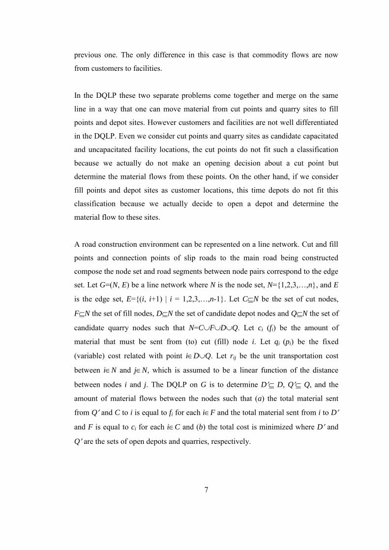
set. Let G=(N, E) be a line network where N is the node set, N={1,2,3,…,n}, and E

is the edge set, E={(i, i+1) | i = 1,2,3,…,n-1}. Let CN be the set of cut nodes,

FN the set of fill nodes, DN the set of candidate depot nodes and QN the set of

candidate quarry nodes such that N=CFDQ. Let ci (fi) be the amount of

material that must be sent from (to) cut (fill) node i. Let qi (pi) be the fixed

(variable) cost related with point iDQ. Let rij be the unit transportation cost

between iN and jN, which is assumed to be a linear function of the distance

between nodes i and j. The DQLP on G is to determine D D, Q Q, and the

amount of material flows between the nodes such that (a) the total material sent

from Q and C to i is equal to fi for each iF and the total material sent from i to D

and F is equal to ci for each iC and (b) the total cost is minimized where D and

Q are the sets of open depots and quarries, respectively.

8

In this study, because of diverse nature of cut and fill operations, stocking function

of depots, and supplying functions of quarries, we assume that C, F, D, and Q are

disjoint sets without loss of generality, and those cost, distance, and supply/demand

parameters are non-negative for simplicity. If “a site” contains multiple features of

operations and functions in a completely different context, then by generating

enough copies of that site, one can develop the disjoint sets as follows. Create a

copy of the site for each different feature and set the distances between these copy

sites to zero on the network representation.

2.2 Literature Review

To the best of our knowledge, neither the road construction literature nor the

location literature contains a study about location decisions in road construction

projects. Nevertheless, there are a few studies on the facility location problems on a

line in the location literature, some of which are formulated as the p-median

problem and/or the fixed charged facility location problem. There are two main

properties that make these facility location problems on a line easier and lead

polynomial or pseudo-polynomial algorithms to solve the problems. The first

property is eligibility of non-fractional allocations of demands to facilities and the

second one is to have identical capacities at all facilities. Having uncapacitated

facilities guarantees the validity of the first property. Love (1976) considers the p-

median problem and proposes a dynamic programming (DP) algorithm to solve the

problem. Brimberg and Revelle (1998) consider the uncapacitated facility location

problem and p-median problem and show that the linear relaxation of their mixed

integer programing (MIP) models gives the integer optimal solution. Berberler et al.

(2011) study the p-median problem on a line and present a DP algorithm. Hsu et al.

(1997) propose an O(pn2) algorithm for solving a facility location problem where n

refers to the number of candidate location sites. The main characteristics of the

problem are a given limit on the number of uncapacitated facilities, location based

fixed costs for the facilities, a unimodal cost function for serving the customers, and

non-fractional allocations of the customers to the facilities. Brimberg and Mehrez

(2001) suggest a DP algorithm to solve the location and sizing problems of

9

facilities. The number, locations, and capacities of facilities and the allocations of

customers to the facilities are determined. Facilities may reach any capacity level at

the expense of a fixed cost, which is a continuous non-decreasing function of the

capacity. As a result of this capacity-cost relation the first property is guaranteed.

Brimberg et al. (2001) investigate the effect of capacity constraints on the location-

allocation problem. In their study the second property is valid and the problem is to

locate at most p homogeneous facilities and to allocate the demand points to the

facilities, such that the sum of fixed and transportation costs is minimized. Demand

nodes and candidate facility locations lie on a line. Facilities may be located at any

point on the line. They propose a DP algorithm when the unit transportation cost

between demand and facility points is an increasing convex function of the

distance. They show that the problem is NP-hard under more general cost

structures. Eben-Chaime et al. (2002) consider a capacitated location-allocation

problem to find the number and locations of capacitated branching facilities and an

allocation of customers to these facilities such that the sum of fixed and allocation

costs is minimized. They propose heuristic solution methods to solve the problem.

Mirchandani et al. (1996) consider a capacitated facility location problem. To serve

a customer, a facility must be located within a given neighborhood of this customer.

Fixed and service costs depend upon their locations on the line. They develop

polynomial time DP algorithms for (i) locating minimum cost facilities to serve all

customers and (ii) maximizing the profit by locating up to p facilities that serve

some or all customers.

The relation between the DQLP and the UFLP is mentioned before. When the

network is a line network, the UFLP is equivalent to the uncapacitated lot sizing

problem with backlogging (ULSPB). So, the DQLP is related with the ULSPB. The

ULSPB is polynomially solvable (see Zangwill 1969; Pochet and Wolsey 2006;

Pochet and Wolsey 1988; Johnson and Montgomery 1974). Zangwill (1969) is the

first to formulate the ULSPB as the network flow problem. He considers concave

cost functions and proposes a backward DP algorithm for the problem. Johnson and

Montgomery (1974) propose a forward DP algorithm for the problem. Pochet and

Wolsey (1988) first formulate the ULSPB as the fixed charge network flow

10

problem. Then they reformulate the problem as the UFLP and the shortest path

problem. They show that the UFLP and the shortest path problem reformulations

are ideal formulations for the ULSPB, i.e., their linear programming relaxations

give the integer optimal solution of the problem. They strengthen the original fixed

charge network flow problem formulation by adding new constraints and propose

separation algorithms for these cutting planes.

In the literature there are several studies that consider the lot sizing problem with

product returns from the customers and/or disposals of excess inventory. The most

generic version of this problem appears in Beltran and Krass (2002), which is a

special case of the DQLP. All other studies add different features on the problem

such as remanufacturing operations for returned products, production capacities,

multi products etc. Note that when backlogging is allowed in the lot sizing problem

with returns and disposals, the resulting problem is equivalent to the DQLP. To the

best of our knowledge, there is no study that considers backlogging.

Another problem that the DQLP is related with is the transportation problem. If

there were no candidate depot and quarry sites (i.e., if there are no decisions for

opening depots and quarries), then the remaining problem would reduce to a

transportation problem defined on a line network. The transportation problem

determines the material flows from the cut points to the fill points such that supply

and demand amounts are balanced and the total transportation cost is minimized.

Note that the transportation problem can be formulated as a linear programming

problem in general and solved by a strongly polynomial algorithm (Nemhauser and

Wolsey, 1988). In our case it is linearly solvable (i.e., O(n)) by using the line

property, given n points. There are several studies that consider the transportation

problem with fixed charged transportation costs between supply and demand points

(see Adlakha and Kowalski, 1999), but according to the best of our knowledge,

there is no study in the literature on transportation problem with location decisions

of both candidate supply and demand points in addition to the initially given (fixed)

supply and demand points.

11

2.3 Fixed Charge Network Flow Problem Formulation of the DQLP

The depot-quarry location problem can be represented as the fixed charge network

flow problem (FNFP) defined on a directed graph G=(N, A) where N={0}N and

A={(i, i+1)| i=1, 2, …, n-1}{(i+1, i)| i=1, 2, ..., n-1}{(0, i)| iQ}{(i, 0)| iD}.

Fixed and variable charges of using arcs (0, i) and (i, 0) in G are equal to qi and pi

values, respectively, where node i corresponds to candidate quarry for the former

case and depot for the latter case. Variable charges of using both arcs (i, i+1) and

(i+1, i) for i=1, 2, ..., n-1 are equal to ri,i+1. The amount of supply (demand) of iC

(F) is equal to ci (fi). Supply (ci) and demand (fi) are zero for iDQ. For node 0,

the supply amount is equal to },0max{

Fi

i

Ci

i fc and the demand amount is equal

to },0max{

Ci

i

Fi

i cf .

Let us define our decision variables for the DQLP. ui (vi) is the amount of forward

(backward) material flow from point i to (i+1) ((i+1) to i) for i=1,…, (n-1). Qi (Di)

is the amount of material obtained (heaped) from (to) quarry (depot) node i for iQ

(iD). yi is equal to 1, if a depot (quarry) is open at a candidate node i, 0 otherwise

for iD (iQ). Figure 2.2 illustrates G for a DQLP instance with n=9, C={3, 8},

F={1, 6, 9}, D={4, 7} and Q={2, 5}.

2

Figure 2.2 G for a DQLP example with n=9.

u1 u7 u2 u3 u4 u5 u6 u8

v2 v3 v4 v5 v6 v7 v8 v1

f9 c3 f1 f6 c8

1 3 5 4 6 7 8 9

Q2 Q5 D4 D7

max{0,

9

1)(

iii

fc } max{0,

9

1)(

iii

cf }

0

(y2) (y4) (y5) (y7)

12

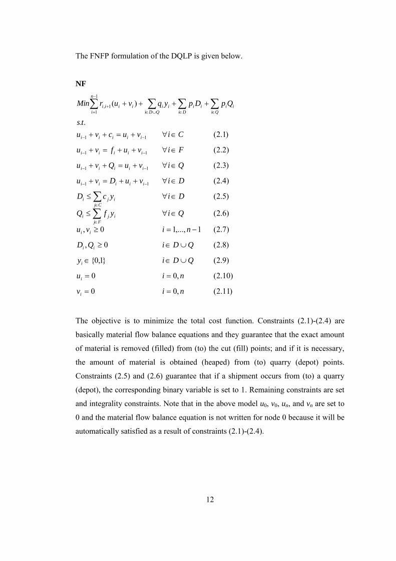
The FNFP formulation of the DQLP is given below.

NF

)11.2(,00

)10.2(,00

)9.2(}1,0{

)8.2(0,

)7.2(1,...,10,

)6.2(

)5.2(

)4.2(

)3.2(

)2.2(

)1.2(..

)(

11

11

11

11

1

11,

niv

niu

QDiy

QDiQD

nivu

QiyfQ

DiycD

DivuDvu

QivuQvu

Fivufvu

Civucvu

ts

QpDpyqvurMin

i

i

i

ii

ii

Fj

iji

Cj

iji

iiiii

iiiii

iiiii

iiiii

Qi

ii

Di

ii

QDi

ii

n

i

iiii

The objective is to minimize the total cost function. Constraints (2.1)-(2.4) are

basically material flow balance equations and they guarantee that the exact amount

of material is removed (filled) from (to) the cut (fill) points; and if it is necessary,

the amount of material is obtained (heaped) from (to) quarry (depot) points.

Constraints (2.5) and (2.6) guarantee that if a shipment occurs from (to) a quarry

(depot), the corresponding binary variable is set to 1. Remaining constraints are set

and integrality constraints. Note that in the above model u0, v0, un, and vn are set to

0 and the material flow balance equation is not written for node 0 because it will be

automatically satisfied as a result of constraints (2.1)-(2.4).

13

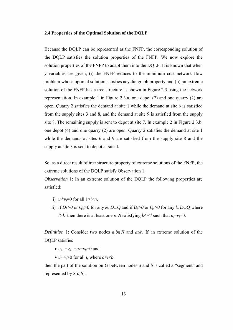
2.4 Properties of the Optimal Solution of the DQLP

Because the DQLP can be represented as the FNFP, the corresponding solution of

the DQLP satisfies the solution properties of the FNFP. We now explore the

solution properties of the FNFP to adapt them into the DQLP. It is known that when

y variables are given, (i) the FNFP reduces to the minimum cost network flow

problem whose optimal solution satisfies acyclic graph property and (ii) an extreme

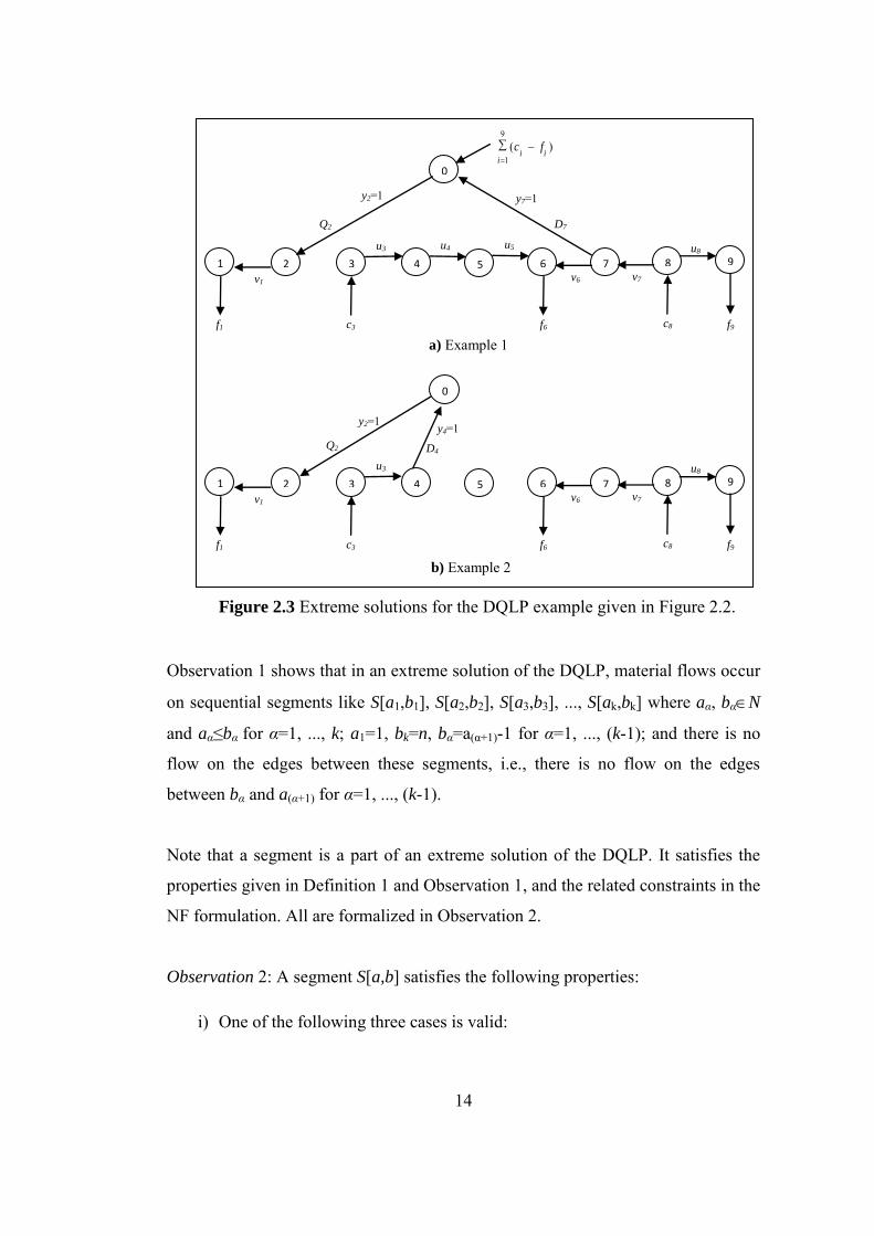
solution of the FNFP has a tree structure as shown in Figure 2.3 using the network

representation. In example 1 in Figure 2.3.a, one depot (7) and one quarry (2) are

open. Quarry 2 satisfies the demand at site 1 while the demand at site 6 is satisfied

from the supply sites 3 and 8, and the demand at site 9 is satisfied from the supply

site 8. The remaining supply is sent to depot at site 7. In example 2 in Figure 2.3.b,

one depot (4) and one quarry (2) are open. Quarry 2 satisfies the demand at site 1

while the demands at sites 6 and 9 are satisfied from the supply site 8 and the

supply at site 3 is sent to depot at site 4.

So, as a direct result of tree structure property of extreme solutions of the FNFP, the

extreme solutions of the DQLP satisfy Observation 1.

Observation 1: In an extreme solution of the DQLP the following properties are

satisfied:

i) ui*vi=0 for all 1≤i<n,

ii) if Dk>0 or Qk>0 for any kDQ and if Dl>0 or Ql>0 for any lDQ where

l>k then there is at least one iN satisfying k≤i<l such that ui=vi=0.

Definition 1: Consider two nodes a,bN and a≤b. If an extreme solution of the

DQLP satisfies

ua-1=va-1=ub=vb=0 and

ui+vi>0 for all i, where a≤i<b,

then the part of the solution on G between nodes a and b is called a “segment” and

represented by S[a,b].

14

Observation 1 shows that in an extreme solution of the DQLP, material flows occur

on sequential segments like S[a1,b1], S[a2,b2], S[a3,b3], ..., S[ak,bk] where aα, bαN

and aα≤bα for α=1, ..., k; a1=1, bk=n, bα=a(α+1)-1 for α=1, ..., (k-1); and there is no

flow on the edges between these segments, i.e., there is no flow on the edges

between bα and a(α+1) for α=1, ..., (k-1).

Note that a segment is a part of an extreme solution of the DQLP. It satisfies the

properties given in Definition 1 and Observation 1, and the related constraints in the

NF formulation. All are formalized in Observation 2.

Observation 2: A segment S[a,b] satisfies the following properties:

i) One of the following three cases is valid:

Figure 2.3 Extreme solutions for the DQLP example given in Figure 2.2.

2

a) Example 1

u3 u4 u5

v6 v7

u8

v1

f9 c3 f1 f6 c8

1 3 5 4 6 7 8 9

Q2 D7

9

1)(

iii

fc

0

y2=1 y7=1

7 2

b) Example 2

u3

v6 v7

u8

v1

f9 c3 f1 f6 c8

1 3 5 4 6 8 9

Q2 D4

0

y2=1 y4=1

15

if

b

Fiai

i

b

Ciai

i fc

then 0

b

Qiai

i

b

Diai

i yy ,

if

b

Fiai

i

b

Ciai

i fc

then 1

b

Diai

iy and 0

b

Qiai

iy , or

if

b

Fiai

i

b

Ciai

i fc

then 0

b

Diai

iy and 1

b

Qiai

iy .

ii) Cut and fill nodes in S[a,b] can partially or entirely satisfy each other’s

demand.

iii) Any iCF where a≤i≤b can receive both or one of the forward and

backward flows. In Figure 2.3.a site 6 receives both of the forward and

backward flows.

iv) In S[a,b], forward and backward flows can be in a mixed order, i.e., they

cannot be separated into two sub parts of S[a,b]. For instance, in Figure

2.3.a, S[3,9] starts with three steps of forward flows, continue with two steps

of backward flows, and ends with a forward flows, which results in three

mixed orders of the flows.

v) Assume that the second or third case in Observation 2.i is valid for S[a,b].

Let us divide S[a,b] into two parts, called left and right parts, assuming an

open depot or quarry in the center of two parts. The material on S[a,b] flows

from one part to other part. For instance, in Figure 2.3.a, the material on

S[3,9] flows from the right to the left as the depot at site 7 is open.

Proposition 1: On a given S[a,b], the optimal amounts of material flow (i) between

its cut and fill nodes, (ii) between its cut nodes and open depot (if any), and (iii)

between its fill nodes and open quarry (if any) plus (iv) the corresponding optimal

total cost can be pre-determined by simple computations.

Proof: Let Dab and Qab be the sets of candidate depot and quarry nodes on S[a,b],

respectively. One of the following three cases occurs according to Observation 2.i:

16

If

b

Fiai

i

b

Ciai

i fc , then there exists no open facility on S[a,b]. The amounts

of material flows on S[a,b] can be computed by using expressions 2.12 and

2.13 for each j where a≤j≤b, due to Observation 1.i.

},0max{

j

Ciai

i

j

Fiai

ij cfv

(2.12)

},0max{

j

Fiai

i

j

Ciai

ij fcu (2.13)

The total cost for S[a,b], TCab, is:

1

1, ||b

aj

j

Ciai

i

j

Fiai

ijjab cfrTC .

If

b

Fiai

i

b

Ciai

i fc , then there exists only one open depot (say at site m). The

amount of material sent to depot m is equal to the difference between the

cut and fill amounts in S[a,b]. Consider depot m as if it would be a fill

node. Thus, we have:

b

Fiai

i

b

Ciai

im fcf , F0= F{m} and modified

expressions (2.12)-(2.13) for each j where a≤j≤b as

},0max{0

j

Ciai

i

j

Fi

ai

ij cfv

(2.12) and

},0max{0

j

Fi

ai

i

j

Ciai

ij fcu (2.13).

The total cost for S[a,b] when depot m is open, is:

1

1, ||)(0

b

uj

j

Ciai

i

j

Fi

ai

ijjmmm

m

ab cfrfpqTC .

Locating a depot on this segment can be decided by first computing m

abTC

values for all mDab and then selecting the location site with the minimal

17

cost value among the computed values. If Dab is an empty set, then a and b

cannot be the first and last nodes of a segment as a part of a candidate

feasible solution and we redefine the total cost term as

,

}{min

ab

abm

abDm

ab

D IfM

D IfTCTC

ab

where M is a very big positive number.

If

b

Fiai

i

b

Ciai

i fc , then there exists only one open quarry (say at site m). The

amount of material obtained from quarry m is equal to the difference

between the cut and fill amounts in S[a,b]. Consider quarry m as if it

would be a cut node. Thus, we have:

b

Ciai

i

b

Fiai

im cfc , C0=C{m} and

modified expressions (2.12)-(2.13) for each j where a≤j≤b as

},0max{0

j

Ci

ai

i

j

Fiai

ij cfv

(2.12) and

},0max{0

j

Fiui

i

j

Ci

ui

ij fcu (2.13).

The total cost for S[a,b] when quarry m is open, is:

1

1, ||)(0

b

aj

j

Ci

ai

i

j

Fiai

ijjmmm

m

ab cfrcpqTC .

Whether locating a quarry on this segment or not can be decided as

follows. First, compute m

abTC values for all mQab and choose the location

site with the minimal cost value. If Qab is an empty set, then a and b cannot

be the first and last nodes of a segment in a candidate feasible solution.

Then, we need to redefine the total cost term as

18

ab

abm

abQm

ab

Q IfM

Q IfTCTC

ab}{min

where M is a very big positive number. □

Let us assume that the first and last nodes of all segments at the optimal solution are

given. Recall that, due to Proposition 1, the “optimal” material flow and location

decisions of a segment can be made. It follows that all the locations and material

flows can be determined if the first and last nodes of each segment are hold by

introducing a (new type) decision (variable). The problem thus reduces to a

decision problem in which the first and last nodes of all segments are determined

subject to minimization of the total cost and the following conditions:

Node 1 is the first node of a segment

Node n is the last node of a segment

If a node is the last node of a segment then the following node is the first

node of the next segment.

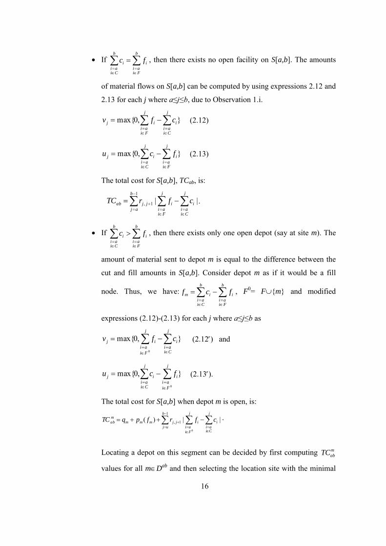
2.5 An Ideal Formulation for the DQLP and a DP Algorithm

Let Zab be equal to 1 if node (a+1) is the first node and b is the last node of a

segment, and 0 otherwise. Using the new decision variable Z, we develop a new

model, called SP, to solve the DQLP:

SP

)15.2(0}1,0{

)14.2(1,...,3,2,1

)13.2(1

)12.2(1

..

min

1

1

0

1

0,

10

1

0 1,1

nbaZ

njZZ

Z

Z

ts

ZTC

ab

n

jb

jb

j

a

aj

n

a

na

n

b

b

n

a

n

ab

abba

19

In the above model the objective function minimizes the total cost of the selected

segments that contain all nodes in the problem network. Constraints (2.12) and

(2.13) guarantee that node 1 is included as the first node of a segment, and node n is

included as the last node of a segment, respectively. Constraint (2.15) guarantees

that if a node is the last node of a segment than the next node is the first node of the

following segment. These three constraints divide the entire line into a set of

sequential, separated, and inclusive segments in a way that every node is included

in exactly one segment.

The above model is equivalent to the mathematical model of the shortest path

problem (SPP). Its linear programming relaxation always gives the integer optimal

solution because of the total unimodularity property of the constraint matrix. For

n=4 the SPP network is given in Figure 2.4.

When the SPP network is analyzed, it is clear that the DQLP can be solved by the

following DP algorithm. Let Gk be the optimal objective function value of the sub-

problem including only the first k nodes.

A DP for the DQLP:

Step 1: From Proposition 1, compute TCab for all 1 ≤ a ≤ b ≤ n.

Step 2: Let G0 = 0. Compute }{min 11 mkmkm

k TCGG

for k = 1, 2, 3, …, n

sequentially. Gn gives the optimal objective value. The optimal solution can be

constructed by backtracking.

TC11 4 0 1 2 3

TC12

TC13

TC14

TC22

TC23

TC24

TC33

TC34

TC44

Figure 2.4 The SPP network for the DQLP with n=4.

20

The DP algorithm is an adaptation of the forward DP algorithm designed for

solving the ULSPB given in Johnson and Montgomery (1974) to the DQLP. The

difference is because of computations of TCab values. The DP algorithm given in

Johnson and Montgomery (1974) solves the ULSPB in O(n3) operations, where n is

the number of periods. The complexity of the above DP algorithm we propose for

the DQLP is O(n3max{|D|, |Q|}).

In addition to the DP algorithm with O(n3) complexity, a better DP algorithm with

O(n2) complexity is proposed for the ULSPB in Pochet and Wolsey (1988) and

Pochet and Wolsey (2006).

In the following section the relations between the DQLP and the ULSPB are

analyzed in detail. We first examine the properties of extreme solutions of the

problems and then provide our findings for differences between the complexities of

solution algorithms.

2.6 Relations between the DQLP and the ULSPB over the Network

The relation between the DQLP and the UFLP is studied in section 2.1. It is

explained that two special cases of the DQLP are equivalent to two instances of the

UFLP defined on a line network with disjoint sets of customer sites and candidate

facility location sites. Then in section 2.2 it is expressed that the UFLP defined on a

line network and the ULSPB defined on a line network are equivalent which is a

well known relation in the literature. So, those two special cases of the DQLP are

also tightly related with the ULSPB defined on a line network. In this section,

besides these two special cases, we deal with the relations between the DQLP and

the ULSPB defined on a line network in general. It is shown that the ULSPB

defined on a line network is a special case of the DQLP. Then the relations between

the DP algorithms developed for these two problems are studied in the complexity

basis.

21

In the ULSPB network, nodes represent the demand and candidate production

periods. There is a fixed setup and a variable production costs related with a

production in a period. Forward flows on the network represent inventories and

backward flows on the network represent backlogs. There are variable (unit)

inventory holding and backlogging costs.

Observation 3:

i) Suppose that D=C=Ø, i.e., there are only quarry sites and fill points, in a

DQLP instance. Thus the remaining problem is equivalent to an instance

of the ULSPB where the nodes in Q (F) correspond to candidate

production (demand) periods. Fixed opening and variable operating costs

for quarry sites correspond to the fixed setup and variable production

costs, respectively, while variable transportation costs on the line network

correspond the variable inventory holding and backlogging costs in the

USLPB. Disjoint sets Q and F of the DQLP implies that demands are zero

for the candidate production periods and no production can be made in

demand periods at the corresponding ULSPB. The fixed setup costs and

variable production costs are set to a very big positive number M in order

to prevent production in demand periods.

ii) Suppose that Q=F=Ø, i.e., there are only depot sites and cut points, in a

DQLP instance. Thus, the remaining problem is equivalent to an instance

of the ULSPB where material flows in the corresponding ULSPB instance

can be considered as if they are from the demand periods to the production

periods.

The ULSPB is solvable in O(n2) time where n is the number of periods. So, the

DQLP instances given in Observation 3 are solvable in O(n2) time. If the objective

function is higher than M in the optimal solution of the corresponding ULSPB

instance, then it shows that there is no feasible solution for the given DQLP

instance (i.e., Q=Ø in the DQLP instance given in Observation 3.i and D=Ø in the

instance given in Observation 3.ii)

22

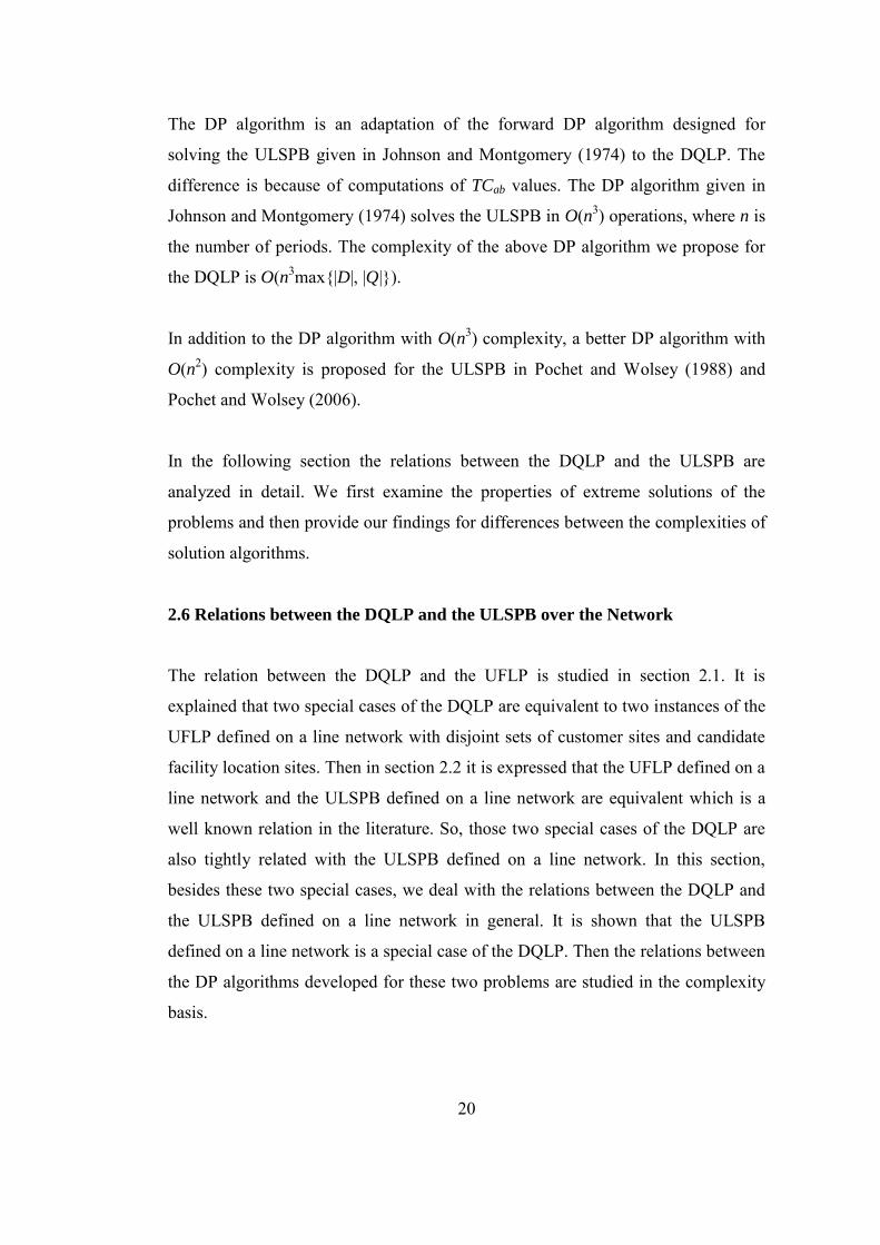
Below we explore whether the ULSPB solution methods are pertinent for the

DQLP.

Any ULSPB instance can be transformed to an instance of the DQLP. Let us

assume a ULSPB instance with set of periods {1, 2, ..., n}. In the ULSPB instances

demand periods and candidate production periods are not assumed to be disjoint.

But they can be separated by duplicating all periods. After copying each element in

the period set, the original periods can be doubled by adding copies into the original

set as {1, 1', 2, 2', ..., n, n'}. The original periods are demand periods. Setup costs

and unit production costs are set to M for these periods where M is a very big

positive number. The copied periods are candidate production periods and demands

associated with these periods are zero. They have fixed setup and unit production

costs. Inventory holding cost and backlogging cost between a period and its copy is

zero. The inventory holding and backlogging costs between period (i') and (i+1) are

equal to the original inventory holding and backlogging costs between periods (i)

and (i+1). Hence the ULSPB instance is reduced to an equivalent instance of the

DQLP where original periods of the ULSPB correspond to fill (cut) points, copied

periods correspond to candidate quarry (depot) sites, inventory holding and

backlogging costs correspond to transportation costs on the line network of the

DQLP, fixed setup costs correspond fixed quarry (depot) opening costs and unit

production costs correspond unit operating costs at quarry (depot) sites. Such

DQLP instances are already specified in Observation 3. By this reverse

transformation it is shown that the ULSPB is a special case of the DQLP. So,

solution methods for the ULSPB are only applicable to the DQLP instances

satisfying Observation 3.

Parts of the extreme solution of the ULSPB corresponding to segments of the

DQLP are called “regeneration interval” in the literature. Therefore, “regeneration

intervals” can be considered as a special case of “segments”. An extreme solution

example for an ULSPB instance with 9 periods is given in Figure 2.5. Considering

the DQLP instances in Observation 3.i (ii) open quarries (depots) correspond to

23

production periods. The corresponding properties of regeneration interval to the

properties of the segment given in Observation 2 are as follows:

Properties of the regeneration interval [a,b]:

i) There is exactly one production period.

ii) All demands in the regeneration interval [a,b] are satisfied from the

production period.

iii) Demand in a period is entirely satisfied by only inventory, production, or

backlogging.

iv) Inventory and backlogging flows are separated on the sub parts of the

regeneration interval. Backlogging flows occur only on the left of the

production period and inventory flows occur only on the right of the

production period for a traditional ULSPB instances. If material flows are

from demand periods to production periods in the considered ULSPB

instance, then backlogging flows occur only on the right of the production

period and inventory flows occur only on the left of the production period

v) There is no flow from the left of production period to the right of it (or

vice versa).

Figure 2.5 An extreme solution example for an ULSPB instance with 9 periods where di is the demand in period i, i = 1, …, 9.

d1 2

d8+d9 d3+d4 d4 d9

d9 d3 d1 d6 d8

1 3 5 4 6 7 8 9

9

1ii

d

0

y2=1 y7=1

d7 d5 d4 d2

d5+d6 d5

4

1ii

d

9

5ii

d

24

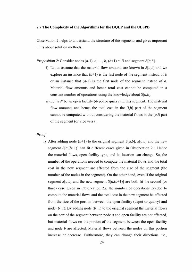
2.7 The Complexity of the Algorithms for the DQLP and the ULSPB

Observation 2 helps to understand the structure of the segments and gives important

hints about solution methods.

Proposition 2: Consider nodes (a-1), a, ...., b, (b+1) N and segment S[a,b].

i) Let us assume that the material flow amounts are known in S[a,b] and we

explore an instance that (b+1) is the last node of the segment instead of b

or an instance that (a-1) is the first node of the segment instead of a.

Material flow amounts and hence total cost cannot be computed in a

constant number of operations using the knowledge about S[a,b].

ii) Let iN be an open facility (depot or quarry) in this segment. The material

flow amounts and hence the total cost in the [i,b] part of the segment

cannot be computed without considering the material flows in the [a,i) part

of the segment (or vice versa).

Proof:

i) After adding node (b+1) to the original segment S[a,b], S[a,b] and the new

segment S[a,(b+1)] can fit different cases given in Observation 2.i. Hence

the material flows, open facility type, and its location can change. So, the

number of the operations needed to compute the material flows and the total

cost in the new segment are affected from the size of the segment (the

number of the nodes in the segment). On the other hand, even if the original

segment S[a,b] and the new segment S[a,(b+1)] are both fit the second (or

third) case given in Observation 2.i, the number of operations needed to

compute the material flows and the total cost in the new segment be affected

from the size of the portion between the open facility (depot or quarry) and

node (b+1). By adding node (b+1) to the original segment the material flows

on the part of the segment between node a and open facility are not affected,

but material flows on the portion of the segment between the open facility

and node b are affected. Material flows between the nodes on this portion

increase or decrease. Furthermore, they can change their directions, i.e.,

25

some forward flows can turn to backward flows or vice versa. So, adding

the node (b+1) to the segment necessitates to calculate all flows and the total

cost on the portion between the open facility and node (b+1). Hence, the

number of the operations in these calculations be affected from the size of

the portion between open facility and node (b+1). For the last situation

assume that original segment fits to the first case given in Observation 2.i.

After adding node (b+1) to the segment, the new segment cannot fit the

same case if (b+1) is a cut or fill point since the total cut and fill amounts

cannot be equal to each other after adding (b+1). This situation is considered

in the initial part of this paragraph. If node (b+1) is a candidate depot or

quarry site, then it cannot be added to original segment S[a,b] as a last node

to obtain a new segment. Since the total cut and fill amounts on the [a,b]

part of the line network are equal to each other, no facility at node (b+1)

will be opened and no material flow will occur between node (b+1) and the

[a,b] portion of the line network. Since the number of operations to

calculate the material flows and the total cost on the new segment is affected

from the segment size it completes the proof for the case adding node (b+1)

to S[a,b] as the last node of the new segment S[a,(b+1)]. Now, the proof for

the case adding node (a-1) to S[a,b] as the first node of the new segment

S[(a-1),b] is trivial.

ii) According to Observation 2.v there can be a material flow from one part of

the segment to the other part. So, such a flow affects the amount of demand

on the opposite part that is satisfied from the open facility (depot or quarry)

and hence the total cost. □

Proposition 2.i is related with the reason of having higher complexity in the DP

algorithm for the DQLP than the DP algorithms for the ULSPB with O(n3)

complexity. Proposition 2.ii is related with the reason of being unable to adapt the

DP algorithm for the ULSPB with O(n2) complexity to the DQLP. In order to

explain the reasons, corresponding properties for the ULSPB to the ones given in

Proposition 2 should be given.

26

Consider an ULSPB instance with n periods. Let pk and dk be unit production cost

and demand in period k, respectively. Let a and b be the first and last periods of a

regeneration interval, respectively, in an ULSPB instance. Let i be the production

period in the regeneration interval and TCab be the total cost associated with the

regeneration interval. Assume that node (b+1) is added as a last period in the

regeneration interval. In this case material flow on the original regeneration interval

is not affected from adding (b+1). All periods in the original regeneration interval

remain as they are to satisfy their entire demands from the production period; the

periods before the production period satisfy their demands by backlogging, the

production period satisfies its demand from itself by production, the periods after

the production period satisfy their demands by inventory. After adding period (b+1)

to the regeneration interval, it satisfies its entire demand from the production period

by inventory. So the total cost in the new situation can be computed by adding the

term (d(b+1)*(pi+hi,(b+1))). Here, hi,(b+1) is the unit inventory holding cost from

production period i to period (b+1). So, the total cost in the new regeneration

interval can be computed in a constant number of operations, which is independent

of the size of the regeneration interval. The case of adding the period (a-1) to the

regeneration interval as the first period is very similar to the case of adding period

(b+1) as the last node. In this new case the additional cost term is (da-1*(pi+s(a-1),i))

where s(a-1),i is the unit backlogging cost from period (a-1) to production period i.

These two cases are the opposite of Proposition 2.i. On the other hand, the material

flows and the total cost on the [i,b] part of the regeneration interval can be

computed without considering the [a,i) part, or vice versa as a result of fifth

property given for regeneration intervals. Also, this is the opposite of Proposition

2.ii. Proposition 2.ii shows that a segment should be considered as a unique block.

But a regeneration interval can be considered as two independent parts according to

the production period.

According to the method explained in the proof of Proposition 1, for a fixed a and b

pair, computing TCab in the DP algorithm for the DQLP requires at most

|}||,max{|*)(* abab QDabK operations, where K is a constant. That is to say,

the complexity of computing TCab is O((b-a)*max{|Dab|, |Qab|}), which requires a

27

number of operations affected by the size of the segment as explained in

Proposition 2.i. Since these computations are done for all pairs of a and b, where

1 ≤ a ≤ b ≤ n, the complexity of Step 1 is O(n3max{|D|, |Q|}). The complexity of

Step 2 is O(n2). Thus, the total complexity of the algorithm is O(n3max{|D|, |Q|}),

which is polynomial.

The complexity of the algorithm for the ULSPB reduces to O(n3) because of the

difference related with Proposition 2.i. Let us reconsider the ULSPB and let a and b

be the first and last nodes of a regeneration interval and i be a production period

(a ≤ i ≤ b). The total cost in the regeneration interval is,

o.w.dspTCdhpTC

bia ifdpqTC

aa ii

i

babibi

i

1-ba ,

iiii

a b )()( ,1

where qi is the fixed setup cost in period t.

For fixed i, we first compute i

abTC for a=b=i and then compute i

abTC values for

fixed a and all b’s greater than i, which require O(n) operations. Note that

computing i

abTC values for all a’s less than i for all (i,b) combinations requires

O(n2) operations. Doing these computations for 1 ≤ i ≤ n requires O(n3) operations

in total in Step 1. In Step 2, O(n2) operations are needed. So, the complexity of the

algorithm is O(n3).

Pochet and Wolsey (1988) and Pochet and Wolsey (2006) use the property of the

ULSPB related with Proposition 2.ii and propose another DP algorithm and another

SPP reformulation. There are O(n) nodes and O(n2) arcs in this SPP reformulation

and the arcs are associated with the corresponding costs on the [a,i), [i], and (i,b]

parts of a regeneration interval. Here, the regeneration interval is divided into three

parts. Computing the costs corresponding to arc lengths requires O(n2) operations

for all (a,i) combinations, O(n) operations for all i, and O(n2) operations for all (i,b)

combinations. So, in total, the ULSPB is converted to a SPP in O(n2) time. Because

the SPP is solvable in O(n2) time, the ULSPB is also solvable in O(n2) time.

28

However, this property is not valid in the DQLP (see Proposition 2.ii). Therefore,

these efficiencies are not applicable to the DQLP.

29

CHAPTER 3

A DYNAMIC LOCATION PROBLEM IN RAILROAD CONSTRUCTION

In this chapter another new location problem, motivated by a real life project,

which appears in the railroad construction projects, is considered. The problem

along with its real life occurrence is explained and studied in detail below.

3.1 Problem Definition

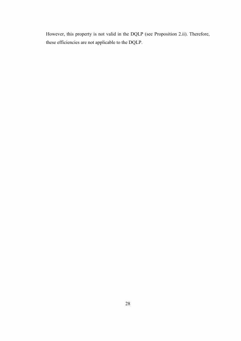
Railroads cannot make sharp curves and must be as smooth as a straight line in both

vertical and horizontal axes because of some technical reasons. Therefore, tunnels

and viaducts, called “art buildings” in the construction terminology, are widely

needed in railroad projects to keep the line straight (see Figure 3.1). The series of

works in a railroad construction project consist of establishing art buildings in

addition to the railroad itself. These buildings are the largest concrete consumption

units in the project. Construction processes of art buildings are summarized below.

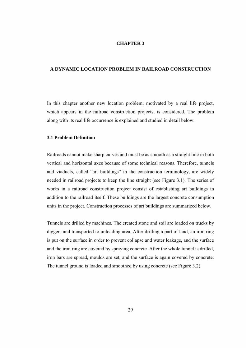
Tunnels are drilled by machines. The created stone and soil are loaded on trucks by

diggers and transported to unloading area. After drilling a part of land, an iron ring

is put on the surface in order to prevent collapse and water leakage, and the surface

and the iron ring are covered by spraying concrete. After the whole tunnel is drilled,

iron bars are spread, moulds are set, and the surface is again covered by concrete.

The tunnel ground is loaded and smoothed by using concrete (see Figure 3.2).

30

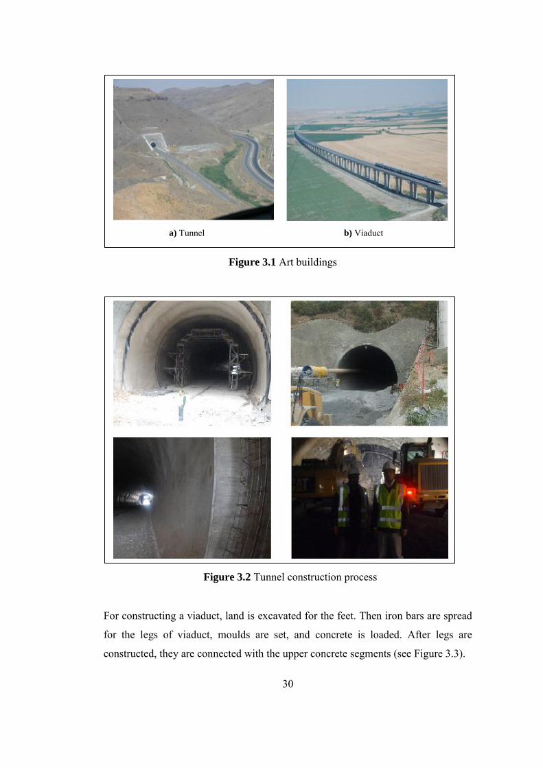
For constructing a viaduct, land is excavated for the feet. Then iron bars are spread

for the legs of viaduct, moulds are set, and concrete is loaded. After legs are

constructed, they are connected with the upper concrete segments (see Figure 3.3).

Figure 3.1 Art buildings

a) Tunnel b) Viaduct

Figure 3.2 Tunnel construction process

31

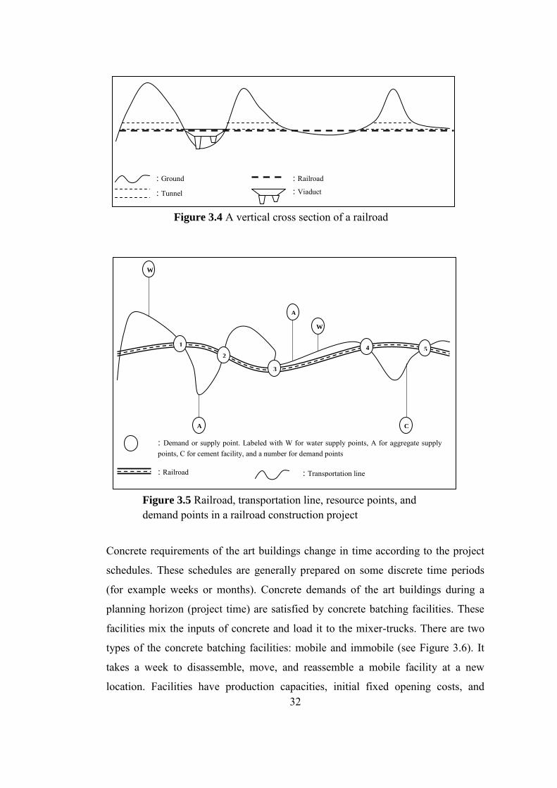
In construction process of a railroad, material handling and transportation activities

are usually performed on a temporary road that lies around the railroad line and

may go around hills and holes. Available water and aggregate (i.e., construction

aggregate, including sand, and pebble) supply points near to the transportation line

would be the candidate input sources while cement would possibly be supplied

from the closest production facility for producing concrete. These supply points

need to be connected to the line with slip roads. In Figure 3.4, an example of a

vertical cross section of a railroad is presented and a panoramic picture from top of

the railroad construction environment of the example is illustrated in Figure 3.5. In

Figure 3.5, the nodes W, A, and C represent alternative water sources, aggregate

supply points, and cement facility, respectively. The nodes labeled with numbers

represent the demand points (of art buildings) of the railroad project shown in

Figure 3.4. An art building can be represented with a single node. If a tunnel or a

viaduct is constructed from the two end points simultaneously, its total concrete

demand should be represented with two separate demand points. In Figure 3.5, for

example, the tunnel on the right is represented with two different demand points,

node 4 and node 5.

Figure 3.3 Viaduct construction process

32

Concrete requirements of the art buildings change in time according to the project

schedules. These schedules are generally prepared on some discrete time periods

(for example weeks or months). Concrete demands of the art buildings during a

planning horizon (project time) are satisfied by concrete batching facilities. These

facilities mix the inputs of concrete and load it to the mixer-trucks. There are two

types of the concrete batching facilities: mobile and immobile (see Figure 3.6). It

takes a week to disassemble, move, and reassemble a mobile facility at a new

location. Facilities have production capacities, initial fixed opening costs, and

: Ground : Viaduct

: Railroad : Tunnel

Figure 3.4 A vertical cross section of a railroad

C

A

A

W

W

1 4

2

3

5

: Demand or supply point. Labeled with W for water supply points, A for aggregate supply points, C for cement facility, and a number for demand points

: Railroad : Transportation line

Figure 3.5 Railroad, transportation line, resource points, and demand points in a railroad construction project

33

monthly operating costs. There are also a fixed cost of transporting a mobile facility

from one site to another and transportation costs of aggregate, water, cement, and

concrete to/from facilities. Generally, the input material sources are uncapacitated.

So, a facility gets input materials from the nearest sources. Demand points (sites of

the art buildings) are also candidate locations for the facilities. The problem is to

determine the number, type, and movement schedule of the mobile facilities, and to

make the concrete production and allocation decisions so that all concrete

requirements are satisfied, facility capacities are not violated, and the total cost is

minimized.

3.2 Literature Review

All studies in the literature on railroad and road construction management mainly

consider scheduling issues. To the best of our knowledge there is no study that

considers location-allocation related issues. There are some studies that consider

road construction and harvesting machine location in timber industry (Epstein et al.

2006), but these problems are very different than the dynamic location problem

discussed so far.

a) Immobile Concrete Batching Facility

Figure 3.6 Concrete batching facilities

b) Mobile Concrete Batching Facility

34

There are a few studies on the facility location problem on a line as discussed in

Chapter 2. Some of them consider the p-median problem and/or the fixed charged

facility location problem (Love 1976, Brimberg and Revelle 1998, Berberler et al.

2011, Hsu et al. 1997, Brimberg and Mehrez 2001, Brimberg et al. 2001, Eben-

Chaime et al. 2002, Mirchandani et al. 1996). For details of the studies in this

category see section 2.2. None of these studies consider dynamic problems and

mobile facilities.

Numerous studies on dynamic location problems in general networks are published

in the literature since Manne (1961, 1967) and Ballou (1968). Time and location

related decisions are mainly on facility opening, closure, reopening, and relocations

(or moves), and capacity reductions, expansions, and partial capacity relocations.

Different combinations of these decisions are considered in the dynamic location

literature. Luss (1982) presents a survey on the capacity expansion problems, which

are related with the dynamic facility location problem. Owen and Daskin (1998)

present a survey on the static and dynamic facility location problems. As successive

works, Melo et al. (2000) review the facility networks, including dynamic ones,

under supply chain management while Klose and Drexl (2005) review studies on

the facility location problems and briefly discuss the dynamic problems. Farahani et

al. (2009) and Arabani and Farahani (2012) are two recent review studies on the

dynamic facility location problem.

Current et al. (1997) classify dynamic location problems in two groups: implicitly

dynamic and explicitly dynamic. Implicitly dynamic problems are “static” in the

sense that all facilities that are to be opened at the beginning of the first period

remain open during the planning horizon. These problems, however, recognize that

parameters may change over time and attempt to account for the effects of these

changes in the initial set of locations. In the explicitly dynamic problems, the

effects of changes are suitably taken into account. For instance, it is possible to

open, reopen, relocate/move, and close the facilities over the planning horizon in

order to response the changes in the parameters. We consider the explicitly

dynamic problems below.

35

We start with clarifying the meaning of some terms like ‘opening and reopening a

facility’ and ‘relocating and moving a facility’ in the literature. In some studies, if

there is a new facility at a location in the current period and there was not any

facility in the previous period at that location, it is treated as if it is being reopening.

Actually, in order to consider the reopening there must be a closed facility in the

previous period and it may restart to operate in the current period. In our study,

‘facility opening’ refers to the situation that a new facility, which was not in the

system before, is added to the system. ‘Facility reopening’ means that an existing

facility that was being closed for a while restarts to operate now. Facility opening

and reopening costs are differentiated because it is expected that opening would be

expensive than reopening. Facility relocation expresses the situation that an existing

facility is closed at a location and a new facility is opened at another location, and

the equipments, materials, etc. in the closed facility are transported to the new

facility. On the other hand, facility moving implies that there is an existing mobile

facility and that existing facility is entirely moved to a new location. Although these

two situations, relocation and moving, are different in semantic and practice, they

can be modeled at a similar structure, which causes misuses of these terms.

However, it is clear that the current locations of facilities must be kept as

information in order to keep track of facility relocation or moving activities. In

addition to this control the previous existence of the facility must be known.

Some studies mainly consider dynamic p-median problems. Wesolowsky (1973)

and Farahani et al. (2009) consider single facility case while Wesolowsky and

Truscott (1975), Galvao and Santibanez-Gonzalez (1992), and Drezner (1995)

consider multi-facility case. For details of these studies see section 4.2.2.

Roodman and Schwarz (1975) study a capacitated dynamic facility location

problem where there are open facilities at the beginning of the first period. It is

assumed that the total demand decreases over the planning horizon and only facility

closures are allowed. A branch and bound (BnB) algorithm is proposed to solve the

problem. Later, Roodman, and Schwarz (1977) extend this problem to one

including facility opening, however, if a facility is opened or closed, its status is

36

unchanged during the rest of the entire horizon. Erlenkotter (1981) considers a

capacity expansion problem under continuous and discrete time assumptions and

presents several heuristics. VanRoy and Erlenkotter (1982) study a dynamic

uncapacitated facility location problem in which new facilities are allowed to be

opened while initially existing facilities are allowed to be closed over the planning

horizon. The objective is to minimize the total discounted costs, including facility

location and operating costs, production and distribution costs. They propose a BnB

with lower bounds obtained through solving linear programming relaxations with a

dual ascent heuristic. Frantzeskakis and Watson-Gandy (1989) study a dynamic

facility location problem where facility opening, closure, and relocation are

allowed. A dynamic programming and BnB based heuristic is presented. Chardaire

et al. (1996) consider a dynamic, uncapacitated facility location problem. Since the

facilities are uncapacitated, each demand point is allocated to the nearest existing

facility in the optimal solution, the problem is to find where and when the facilities

are opened such that the summation of facility opening and operating costs, and

allocation cost is minimized. They develop a quadratic mixed integer programming

model and propose a Lagrangian relaxation in order to find a lower bound and a

simulated annealing heuristic to obtain good solutions in a reasonable time. Gama

and Captivo (1998) consider a problem in which only facility opening and closure

is possible. They propose a two phase heuristic approach to solve the problem. The

first phase is “drop” phase. In this phase, first, it is assumed that there is a facility at

all nodes in all periods, then some facilities are dropped. The second phase is a

local search phase. In this phase, the solution at the end of the first phase is tried to

be improved. Torres-Soto and Üster (2011) consider two dynamic capacitated

facility location problems. In the first problem new facilities can be opened and/or

existing facilities can be closed in a period. In the second problem all facilities are

to be located in the first period and open during the planning horizon. They propose

Lagrangian relaxation and Bender’s decomposition algorithms for the first problem

and a Bender’s decomposition algorithm for the second problem. Sambola et al.

(2009) introduce a dynamic location problem and call it as the multi-period

incremental service facility location problem. In this problem a predetermined

number of facilities are to be opened in each period. In any period, there is a lower

37

limit on the number of customers assigned to the open facilities. All customers must

be assigned to a facility until the end of horizon. The objective is to minimize the

sum of assignment and facility opening costs. They propose a Lagrangian heuristic

to solve the problem. Sambola et al. (2010) try to develop strong formulations for

the multi-period incremental service facility location problem and propose three

models for this purpose. Besides facility opening and capacity expansion, facility

closure and capacity reduction are studied in Antunes and Peeters (2000 and 2001).

They use a simulated annealing algorithm to solve the problem. Shulman (1991)

considers a dynamic facility location/capacity expansion problem. There are

multiple type facilities with different capacities. Only facility opening is allowed.

The problem consists of facility opening decisions on type, time, and location basis.

The author presents a Lagrangean heuristic to solve the problem. Lim and Kim

(1999) consider a dynamic capacitated facility location problem in which the

capacities are determined via acquisition and/or disposal of multiple type modular

capacity alternatives. There are multi-type products that require different set of

operations. While deciding on the facility locations and capacity plans, it is required

to satisfy the needs of these operations. A heuristic procedure based on Lagrangian

relaxation and branch and cut algorithm is proposed to solve the problem. Gourdin

and Klopfenstein (2008) develop an integer programming model for the dynamic

concentrator location problem. Several capacitated concentrators and modules

between terminals and concentrators can be opened at any period, but they cannot

be closed or moved. The objective is to minimize the total investment cost of

concentrators and modules. They perform polyhedral analysis, develop facet

defining inequalities, and present numerical results.

There are several studies that consider reopening of existing but currently being

close facilities. The opening and reopening costs are distinguished. Dias et al.

(2006) propose a primal-dual heuristic to solve three different dynamic facility

location problems with opening, closure, and reopening of facilities. In the first

problem there is an upper limit on facility capacity. In the second problem, the total

demand allocated to a facility must be in between its minimum and maximum

capacities. In the third problem, facilities have an initial (start up) maximum

38

capacity, which decreases during its operating periods. The objective is to minimize

the total facility opening, reopening, and customer allocation costs. Dias et al.

(2007) study a very similar problem in which facilities can be opened, closed, and

reopened, but partial allocations are not allowed. Authors propose a primal-dual

heuristic and a branch and bound algorithm to solve the problem.

As far as we are aware of, there is no locational study considering the application

area of our problem. It has own unique properties such as having a line network

structure and a dynamic demand nature. There are few studies considering mobile

facilities in the literature. However, there is no study considering mobile and

immobile facilities simultaneously as we are dealing with. We differentiated

abolishing a facility than closing one. A closed facility is the one being not operated

until reopening in future over the planning horizon. However, if a facility is

abolished, then it is assumed to be permanently removed away from the system

until the end of the planning horizon. We assume that opening, abolishing, or

moving of a facility may occur more than once in the same location over the

planning horizon. In the case study problem, we consider that a facility can be

opened at a location and then can be moved to another location or abolished. Note

that closing a facility in a period and then reopening in the next period can be an

economic option because of changes on demand quantities. These events may

repeat several times over the horizon.

In the following section, two mathematical models are given to solve the problem.

Adaptation of the models to the similar problems in the literature is also discussed.

3.3 Two MIP formulations for the Problem

Consider a set of points, D, on a line representing actual demand and candidate

location sites. Let T be the number of periods in the planning horizon and dit be

concrete demand of point Di in period t, t = 1, ..., T. Let CS (CF) be a fixed

construction cost of a(n) (im)mobile facility. Let TCS be a fixed moving cost of a

mobile facility, including costs of disassembly, transportation to the new location,

39

and reassembly. Note that distance based transportation costs of mobile facilities

are assumed to be negligible since the main component of moving cost is due to

disassembly and reassembly operations. Since it takes time to relocate a facility, we

define ρ as the percent of time on a period needed to relocate a mobile facility. It is

assumed that moving a mobile facility does not take longer than a period. Let KS

(KF) be concrete production capacity of a(n) (im)mobile facility in a period. There

is a fixed facility operating cost in a period, OC, which includes labor costs, loader

rents, maintenance costs, and rents of the facility.

Concrete should be transported from facility to demand points within two hours;

otherwise it cannot be used anymore. Therefore, given 35 km/hour average speed of

a loaded mixer-truck carrying concrete, the maximum distance from facilities to

demand points cannot exceed 70 km. Let rij be 1 if the distance between points i

and j is equal to or less than 70 km, 0 otherwise. Suppliers of input materials are

uncapacitated. Therefore, a facility gets all needed inputs from the cheapest

suppliers. The amounts of input materials to produce one ton concrete are known.

Thus, the amounts of input material received from the suppliers and their total input

material transportation costs can be computed for a candidate facility location. Let

Gij be the total cost of input materials needed to produce one ton concrete at Di

and transporting the concrete from Di to Dj . Below we present the first

mixed integer programming (MIP) model, called M1, to solve the problem. In this

model, in order to use small number of binary variables, an artificial “pool” is

assumed for mobile facilities and mobile facility movements are managed by using

this pool. Thus, mobile facility movements are controlled by decision variables

with two indices.

Decision Variables

SVit: 1 if a mobile facility is available at Di in t, 0 otherwise.

FVit: 1 if an immobile facility is available at Di in t, 0 otherwise.

Sit: 1 if a mobile facility is opened at Di in t, 0 otherwise.

Fit: 1 if an immobile facility is opened at Di in t, 0 otherwise.

40

FAit: 1 if an available immobile facility at Di is abolished in t, 0 otherwise.

SAt: the number of mobile facilities abolished in t.

SComit: 1 if an available mobile facility at somewhere moves to Di in t, 0

otherwise.

SGoit: 1 if an available mobile facility at Di moves to somewhere in t, 0

otherwise.

xijt: the amount of concrete transported from Di to Dj in t (ton).

M1

)14.3(1,0

)13.3(1}1,0{

)12.3(20

)11.3(2}10{

)10.3(11

)9.3(1,)(*

)8.3(1

)7.3(1

)6.3(2

)5.3(

)4.3(2

)3.3(2

)2.3(..

(3.1) **

))(***(min

1

11

1

11

12

1

,...,TD, tjix

,...,TD, ti,FV,SV,FS

,...,TtSA

,...,TD, ti,,FA,SGoSCom

,...,TD, tiSVFV

,...,TD, tjiSVFVdx

,...,TD, tjd*xr

,...,TD, ti *KS*SComKF*FVKS*SVx

,...,TD, tiFAFVFVF

DiFVF

,...,TtSASComSGo

,...,TD, tiSGoSVSComSVS

DiSVS

ts

xGSComTCS

FVSVOCFCFSCS

ijt

itititit

t

ititit

itit

ititjtijt

jt

Di

ijtij

ititit

Dj

ijt

ititi,tit

ii

t

Di

it

Di

it

itititi,tit

ii

Di Dj

T

t

ijtij

Di

T

t

it

itititit

Di

T

t

In this model, (3.1) minimizes the total cost. Constraints (3.2) and (3.3) provide

whether a mobile facility exists at Di in period t or not. Constraint (3.4) ensures

the balance of mobile facilities at a period. It is assumed that there is a pool of

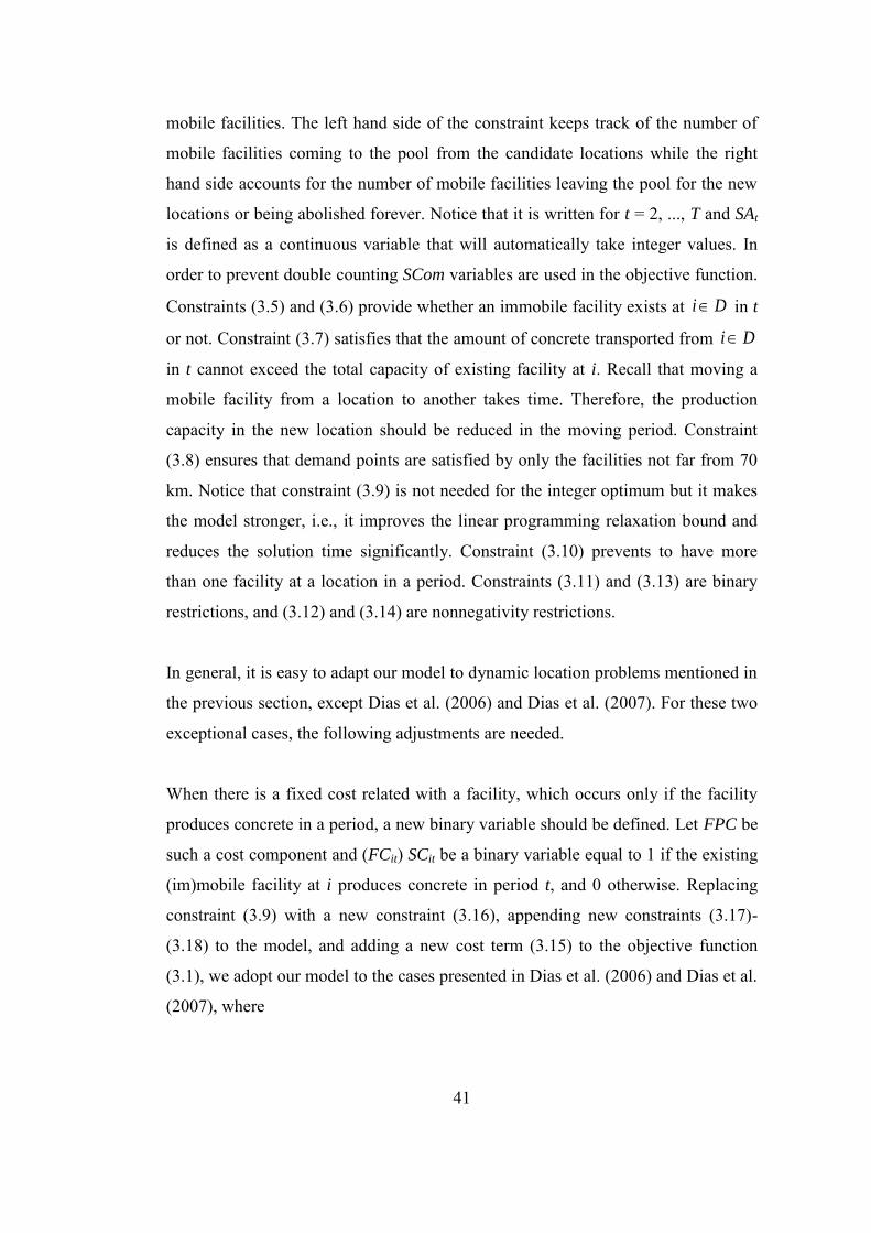
41

mobile facilities. The left hand side of the constraint keeps track of the number of

mobile facilities coming to the pool from the candidate locations while the right

hand side accounts for the number of mobile facilities leaving the pool for the new

locations or being abolished forever. Notice that it is written for t = 2, ..., T and SAt

is defined as a continuous variable that will automatically take integer values. In

order to prevent double counting SCom variables are used in the objective function.

Constraints (3.5) and (3.6) provide whether an immobile facility exists at Di in t

or not. Constraint (3.7) satisfies that the amount of concrete transported from Di

in t cannot exceed the total capacity of existing facility at i. Recall that moving a

mobile facility from a location to another takes time. Therefore, the production

capacity in the new location should be reduced in the moving period. Constraint

(3.8) ensures that demand points are satisfied by only the facilities not far from 70

km. Notice that constraint (3.9) is not needed for the integer optimum but it makes

the model stronger, i.e., it improves the linear programming relaxation bound and

reduces the solution time significantly. Constraint (3.10) prevents to have more

than one facility at a location in a period. Constraints (3.11) and (3.13) are binary

restrictions, and (3.12) and (3.14) are nonnegativity restrictions.

In general, it is easy to adapt our model to dynamic location problems mentioned in

the previous section, except Dias et al. (2006) and Dias et al. (2007). For these two

exceptional cases, the following adjustments are needed.

When there is a fixed cost related with a facility, which occurs only if the facility

produces concrete in a period, a new binary variable should be defined. Let FPC be

such a cost component and (FCit) SCit be a binary variable equal to 1 if the existing

(im)mobile facility at i produces concrete in period t, and 0 otherwise. Replacing

constraint (3.9) with a new constraint (3.16), appending new constraints (3.17)-

(3.18) to the model, and adding a new cost term (3.15) to the objective function

(3.1), we adopt our model to the cases presented in Dias et al. (2006) and Dias et al.

(2007), where

42

)18.3(,

)17.3(,

)16.3(,,)(*

)15.3()(*1

T1,...,tDiSVSC

T1,...,tDiFVFC

T1,...,tDjiSCFCdx

SCFCFPC

itit

itit

ititjtijt

Di

T

t

itit

Note that we differentiate closing a facility from abolishing it. In Dias et al. (2006)

and Dias et al. (2007) when a closed facility is reopened, a fixed reopening cost is

charged. In order to capture this property (for immobile facilities) in our model, a

new binary variable, FRit, which is equal to 1 if a closed immobile facility at i is

reopened in t and 0 otherwise, is needed. Also, besides the above changes,

constraint (3.19) must be added to the model.

)19.3(221,1, T,...,t D,i FRFCFCFVFV i ttii ttii t

A similar modification can be made for mobile facilities, together with introducing

appropriate cost components to be added to the objective function. If partial

capacity relocation and/or capacity extension/reduction are allowed, it is enough to

relax integrality restrictions on binary variables.

In our preliminary studies we saw that M1 solves the problems in long times and

we developed a new model, called M2. Artificial mobile facility pool approach is

left in the new model and movements are controlled by new decision variables with

three indices. With this new manner the number of binary variables increases

significantly, however, since the origin-destination node information is introduced

into the definition of the decision variable, the movements are now tracked directly.

M2 is given below.

Let SKijt be a binary variable such that it is equal to 1 if an available mobile facility

is moved from Di to Dj in t, 0 otherwise. SAit is 1 if an available mobile

facility at Di is abolished in t, 0 otherwise.

43

M2

(3.24)2}1,0{

(3.23)1,|}1,0{

(3.22)1

(3.21)2)14.3(),13.3(),10.3()8.3(),6.3(),5.3(),2.3(

..

(3.20) **

))(***(min

\

\\1

1}{\ 2

1

,...,TD, ti,FASA

,...,T tjiDi,jSK

,...,TD, tiSK *KS*KF*FVKS*SVx

,...,TD, tiSASKSVSKSVS

ts

xGSKTCS

FVSVOCFCFSCS

itit

ijt

{i}Dj

jititit

Dj

ijt

it

{i}Dj

ijtit

{i}Dj

jiti,tit

Di Dj

T

t

ijtij

Di iDj

T

t

ijt

itititit

Di

T

t

In this model, (3.20) minimizes the total cost. Constraints (3.2), (3.5), (3.6), (3.8)-

(3.10), (3.13) and (3.14) are explained before. Constraints (3.21) provide whether a

mobile facility exists at Di in period t or not. Constraint (3.22) satisfies that the

amount of concrete transported from Di in t cannot exceed the total capacity of

existing facility at i. Since moving a mobile facility from a location to another takes

time, the production capacity in the new location should be reduced in the moving

period.

The adaptation of M1 to the similar problems in the literature is explained above.

Note that these steps are related with the common parts of M1 and M2. Thus, those

steps specified for M1 are also valid for M2.

3.4 A Preprocessing Heuristic to Reduce the Number of Candidate Sites

As expected, solving the large size problems using MIP formulations is not

practical because it takes too much time as the problem size continues to grow.

Besides it causes memory problems at the computing environment. In order to find

good solutions to large size problems in reasonably short running times, a

concentration heuristic is proposed. The heuristic reduces the entire candidate

location set into a small “attractive” subset in order to decrease the input size of the

44

formulation. The heuristic first partitions the planning horizon into a set of

“aggregated” periods, each of which combines a number of consecutive (original)

periods into a single (whole) period. Then it solves these single period problems

independently for a facility type to determine the best candidate location sites for

that particular facility type. The heuristic uses a single parameter to set the

number of consecutive periods to be aggregated into a single period. We assume

that is set as being capable to divide T with no remainder. The new single period

problem is formulated as a revised version of M1 and M2 and presented below as a

part of the heuristic.

Preprocessing heuristic for any facility type

Step 1: Define S as the set of candidate sites. S = Ø;

Compute

t

tu

iuit ddθ

1)1(θ

' for all Di and t =1,…,T/.

Step 2: FFOC = Facility construction cost + *fixed operation cost;

PC = *Facility capacity.

Step 3: t =1

Step 4: Solve the following single period problem, called Problemt for t

Problemt

)30.3(}1,0{

)29.3(,0

)28.3(*

)27.3(*'

)26.3('*..

(3.25)**min

Diy

Djix

DiyPCx

Diydx

Djdxr

ts

xGyFFOC

i

ijt

Dj

iijt

ijtijt

jt

Di

ijtij

Di Dj

ijtij

Di

i

Let Yt={i | yi=1 at the optimal solution of Problemt};

S = S Yt

Step 5: If t<T/, then t = t+1 and go to Step4. Otherwise, stop.

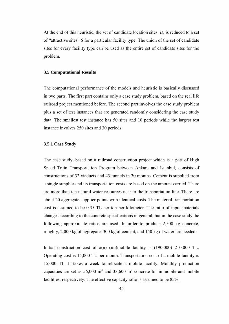
45

At the end of this heuristic, the set of candidate location sites, D, is reduced to a set

of “attractive sites” S for a particular facility type. The union of the set of candidate

sites for every facility type can be used as the entire set of candidate sites for the

problem.

3.5 Computational Results

The computational performance of the models and heuristic is basically discussed

in two parts. The first part contains only a case study problem, based on the real life

railroad project mentioned before. The second part involves the case study problem

plus a set of test instances that are generated randomly considering the case study

data. The smallest test instance has 50 sites and 10 periods while the largest test

instance involves 250 sites and 30 periods.

3.5.1 Case Study

The case study, based on a railroad construction project which is a part of High

Speed Train Transportation Program between Ankara and İstanbul, consists of

constructions of 32 viaducts and 43 tunnels in 30 months. Cement is supplied from

a single supplier and its transportation costs are based on the amount carried. There

are more than ten natural water resources near to the transportation line. There are

about 20 aggregate supplier points with identical costs. The material transportation

cost is assumed to be 0.35 TL per ton per kilometer. The ratio of input materials

changes according to the concrete specifications in general, but in the case study the

following approximate ratios are used. In order to produce 2,500 kg concrete,

roughly, 2,000 kg of aggregate, 300 kg of cement, and 150 kg of water are needed.

Initial construction cost of a(n) (im)mobile facility is (190,000) 210,000 TL.

Operating cost is 15,000 TL per month. Transportation cost of a mobile facility is

15,000 TL. It takes a week to relocate a mobile facility. Monthly production

capacities are set as 56,000 m3 and 33,600 m3 concrete for immobile and mobile

facilities, respectively. The effective capacity ratio is assumed to be 85%.

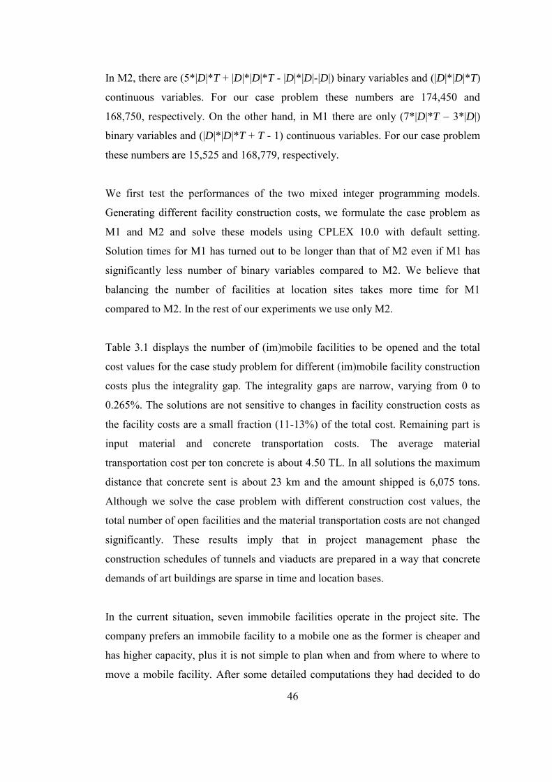
46

In M2, there are (5*|D|*T + |D|*|D|*T - |D|*|D|-|D|) binary variables and (|D|*|D|*T)

continuous variables. For our case problem these numbers are 174,450 and

168,750, respectively. On the other hand, in M1 there are only (7*|D|*T – 3*|D|)

binary variables and (|D|*|D|*T + T - 1) continuous variables. For our case problem

these numbers are 15,525 and 168,779, respectively.

We first test the performances of the two mixed integer programming models.

Generating different facility construction costs, we formulate the case problem as

M1 and M2 and solve these models using CPLEX 10.0 with default setting.

Solution times for M1 has turned out to be longer than that of M2 even if M1 has

significantly less number of binary variables compared to M2. We believe that

balancing the number of facilities at location sites takes more time for M1

compared to M2. In the rest of our experiments we use only M2.

Table 3.1 displays the number of (im)mobile facilities to be opened and the total

cost values for the case study problem for different (im)mobile facility construction

costs plus the integrality gap. The integrality gaps are narrow, varying from 0 to

0.265%. The solutions are not sensitive to changes in facility construction costs as

the facility costs are a small fraction (11-13%) of the total cost. Remaining part is

input material and concrete transportation costs. The average material

transportation cost per ton concrete is about 4.50 TL. In all solutions the maximum

distance that concrete sent is about 23 km and the amount shipped is 6,075 tons.

Although we solve the case problem with different construction cost values, the

total number of open facilities and the material transportation costs are not changed

significantly. These results imply that in project management phase the

construction schedules of tunnels and viaducts are prepared in a way that concrete

demands of art buildings are sparse in time and location bases.

In the current situation, seven immobile facilities operate in the project site. The

company prefers an immobile facility to a mobile one as the former is cheaper and

has higher capacity, plus it is not simple to plan when and from where to where to

move a mobile facility. After some detailed computations they had decided to do

47

so. All facilities had been constructed in the first period and would operate until the

end of the horizon. For benchmarking we have fixed the locations according to the

current facility configuration and found the best allocations using the same cost

setting. Resulting total cost was 32,962,952 TL, and is about 10% higher than the

cost of suggested solution in Table 3.1. In our solution, four mobile and two

immobile facilities are located and mobile facilities are relocated 18 times over the

horizon. We have examined their solution as if one of seven facilities is closed

without changing facility configuration, and found out that they could save about

700,000 TL if it wasn’t opened.

Table 3.1 Number of open facilities, solution values by M2, and deviation of the

solution value by M2 relative to the linear solution to M2 for the case study

problem with varying costs†

CF

CS

110 150 190

#P Obj G(LP) #P Obj G(LP) #P Obj G(LP)

110 5 m 29,369 0.212 6 29,397* 0.265 6 29,397* 0.265 1 i 0 0

130 4 29,460 0.196 5 29,509 0.237 6 29,517* 0.262 2 1 0

150 3 29,524 0.133 5 29,609 0.202 6 29,637* 0.261 3 1 0

170 2 29,574 0.071 4 29,700 0.179 5 29,749 0.235 4 2 1

190 2 29,614 0.011 3 29,764 0.012 5 29,849* 0.200 4 3 1

210 2 29,654 0.000 2 29,814 0.061 4 29,940 0.177 4 4 2

†CS (CF) stands for construction cost of a(n) (im)mobile facility (in 1,000 TL); #P indicates the number of open facilities where m(i) stands for the number of (im)mobile facilities; “Obj” indicates the best integer solution value by M2 (in 1,000

TL); and G(LP)=100(Obj-LS)/Obj, where LS indicates the linear solution to M2 refers to the integrality gap (i.e., deviation of

the best integer solution relative to the linear solution to M2) for M2. CPLEX 10.0 with default setting runs until the gap between the best solution and the lower bound less than or equal to 0.01% unless memory usage reaches to its limitation.

Results of the runs that exceed the memory limit are indicated by *.

In the next experiment we have solved the original problem with a few different

movement costs between 15,000 TL and 9,000 TL to see the effects of mobile

facility movement cost. When fixed movement cost of a mobile facility decreases,

the mobile facilities get more favorable as it is expected. The total cost reduces

since facilities get closer to demand nodes as the number of movements increases.

Results are given in Table 3.2, where the (im)mobile facility construction cost is

(190,000) 210,000 TL.

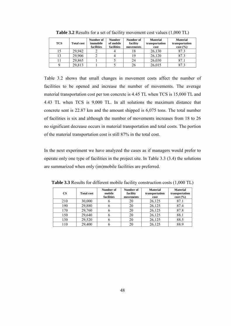
48

Table 3.2 Results for a set of facility movement cost values (1,000 TL)

TCS Total cost

Number of

immobile

facilities

Number

of mobile

facilities

Number of

facility

movements

Material

transportation

cost

Material

transportation

cost (%)

15 29,942 2 4 18 26,130 87.3 13 29,906 2 4 19 26,120 87.3 11 29,865 1 5 24 26,030 87.1 9 29,813 1 5 26 26,015 87.3

Table 3.2 shows that small changes in movement costs affect the number of

facilities to be opened and increase the number of movements. The average

material transportation cost per ton concrete is 4.45 TL when TCS is 15,000 TL and

4.43 TL when TCS is 9,000 TL. In all solutions the maximum distance that

concrete sent is 22.87 km and the amount shipped is 6,075 tons. The total number

of facilities is six and although the number of movements increases from 18 to 26

no significant decrease occurs in material transportation and total costs. The portion

of the material transportation cost is still 87% in the total cost.

In the next experiment we have analyzed the cases as if managers would prefer to

operate only one type of facilities in the project site. In Table 3.3 (3.4) the solutions

are summarized when only (im)mobile facilities are preferred.

Table 3.3 Results for different mobile facility construction costs (1,000 TL)

CS Total cost

Number of

mobile

facilities

Number of

facility

movements

Material

transportation

cost

Material

transportation

cost (%)

210 30,000 6 20 26,125 87.1 190 29,880 6 20 26,125 87.4 170 29,760 6 20 26,125 87.8 150 29,640 6 20 26,125 88.1 130 29,520 6 20 26,125 88.5 110 29,400 6 20 26,125 88.9

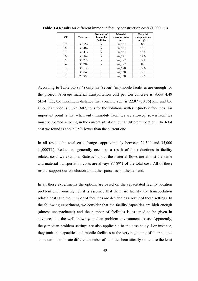
49

Table 3.4 Results for different immobile facility construction costs (1,000 TL)

CF Total cost

Number of

immobile

facilities

Material

transportation

cost

Material

transportation

cost (%)

190 30,557 7 26,887 88 180 30,487 7 26,887 88.1 170 30,417 7 26,887 88.4 160 30,347 7 26,887 88.6 150 30,277 7 26,887 88.8 140 30,207 7 26,887 89 130 30,130 8 26,690 88.6 120 30,045 9 26,520 88.3 110 29,955 9 26,520 88.5

According to Table 3.3 (3.4) only six (seven) (im)mobile facilities are enough for

the project. Average material transportation cost per ton concrete is about 4.49

(4.54) TL, the maximum distance that concrete sent is 22.87 (30.86) km, and the

amount shipped is 6,075 (607) tons for the solutions with (im)mobile facilities. An

important point is that when only immobile facilities are allowed, seven facilities

must be located as being in the current situation, but at different location. The total

cost we found is about 7.5% lower than the current one.

In all results the total cost changes approximately between 29,500 and 35,000

(1,000TL). Reductions generally occur as a result of the reductions in facility

related costs we examine. Statistics about the material flows are almost the same

and material transportation costs are always 87-89% of the total cost. All of these

results support our conclusion about the sparseness of the demand.

In all these experiments the options are based on the capacitated facility location

problem environment, i.e., it is assumed that there are facility and transportation

related costs and the number of facilities are decided as a result of these settings. In

the following experiment, we consider that the facility capacities are high enough

(almost uncapacitated) and the number of facilities is assumed to be given in

advance, i.e., the well-known p-median problem environment exists. Apparently,

the p-median problem settings are also applicable to the case study. For instance,

they omit the capacities and mobile facilities at the very beginning of their studies

and examine to locate different number of facilities heuristically and chose the least

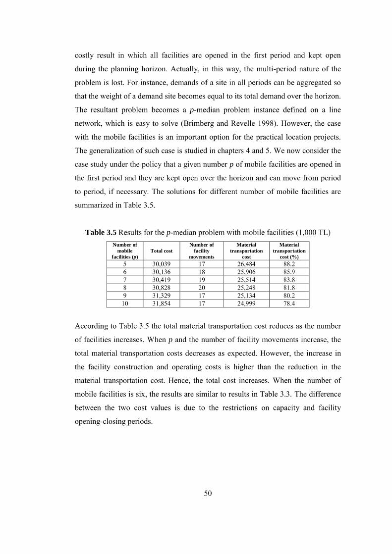
50

costly result in which all facilities are opened in the first period and kept open

during the planning horizon. Actually, in this way, the multi-period nature of the

problem is lost. For instance, demands of a site in all periods can be aggregated so

that the weight of a demand site becomes equal to its total demand over the horizon.

The resultant problem becomes a p-median problem instance defined on a line

network, which is easy to solve (Brimberg and Revelle 1998). However, the case

with the mobile facilities is an important option for the practical location projects.

The generalization of such case is studied in chapters 4 and 5. We now consider the

case study under the policy that a given number p of mobile facilities are opened in

the first period and they are kept open over the horizon and can move from period

to period, if necessary. The solutions for different number of mobile facilities are

summarized in Table 3.5.

Table 3.5 Results for the p-median problem with mobile facilities (1,000 TL) Number of

mobile

facilities (p)

Total cost

Number of

facility

movements

Material

transportation

cost

Material

transportation

cost (%)

5 30,039 17 26,484 88.2 6 30,136 18 25,906 85.9 7 30,419 19 25,514 83.8 8 30,828 20 25,248 81.8 9 31,329 17 25,134 80.2

10 31,854 17 24,999 78.4

According to Table 3.5 the total material transportation cost reduces as the number

of facilities increases. When p and the number of facility movements increase, the

total material transportation costs decreases as expected. However, the increase in

the facility construction and operating costs is higher than the reduction in the

material transportation cost. Hence, the total cost increases. When the number of

mobile facilities is six, the results are similar to results in Table 3.3. The difference

between the two cost values is due to the restrictions on capacity and facility

opening-closing periods.

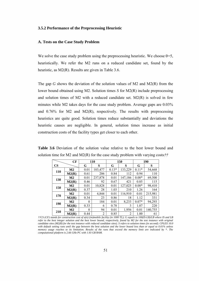
51

3.5.2 Performance of the Preprocessing Heuristic

A. Tests on the Case Study Problem

We solve the case study problem using the preprocessing heuristic. We choose =5,

heuristically. We refer the M2 runs on a reduced candidate set, found by the

heuristic, as M2(R). Results are given in Table 3.6.

The gap G shows the deviation of the solution values of M2 and M2(R) from the

lower bound obtained using M2. Solution times S for M2(R) include preprocessing

and solution times of M2 with a reduced candidate set. M2(R) is solved in few

minutes while M2 takes days for the case study problem. Average gaps are 0.03%

and 0.76% for M2 and M2(R), respectively. The results with preprocessing

heuristics are quite good. Solution times reduce substantially and deviations the

heuristic causes are negligible. In general, solution times increase as initial

construction costs of the facility types get closer to each other.

Table 3.6 Deviation of the solution value relative to the best lower bound and

solution time for M2 and M2(R) for the case study problem with varying costs††

CF

CS

110 150 190

G S G S G S

110 M2 0.01 103,477 0.13* 133,229 0.11* 54,668

M2(R) 0.61 206 0.84 112 0.94 110

130 M2 0.01 237,878 0.01 147,186 0.08* 69,500

M2(R) 0.46 92 0.67 421 0.85 115

150 M2 0.01 10,828 0.01 127,025 0.08* 98,410

M2(R) 0.37 28 1.03 210 1.26 164

170 M2 0.01 4,844 0.01 116,910 0.01 215,981

M2(R) 0.34 23 0.86 18 1.12 331

190 M2 0 184 0.01 8,233 0.07* 94,293

M2(R) 0.33 6 0.78 3 1.07 220

210 M2 0 94 0.01 1,956 0.01 140,755

M2(R) 0.44 2 0.85 2 1.00 61 ††CS (CF) stands for construction cost of a(n) (im)mobile facility (in 1000 TL); G equals to 100(IS-LB)/LB where IS and LB

refer to the best integer solution and the best lower bound, respectively, found by M2 for the test instance with original

candidate sites (M2(R) for the test instance with reduced candidate sites). S refers to solution times (in second). CPLEX 10.0

with default setting runs until the gap between the best solution and the lower bound less than or equal to 0.01% unless memory usage reaches to its limitation. Results of the runs that exceed the memory limit are indicated by *. The

computational platform is 2.66 GHz PC with 1.93 GB RAM.

52

B. Tests on the Randomly Generated Test Instances

In total 90 test problem instances are generated by the procedure explained in

Appendix A. We use two stopping criteria in our computational experiment. A run

is finished if its solution time exceeds 3 hours and its gap is smaller than 1.0%, or if

the available memory limit is exceeded. We choose =5 heuristically. All

computational results on the randomly generated problem instances are given in

Table 3.7.

According to the results given in Table 3.7, feasible solutions cannot be found 23

times out of 90 by M2 and two times by M2(R). Overall average gaps are 0.47%

and 1.53% for 67 test instances solved by M2 and M2(R), respectively. Average

solution times are 35 minutes and 4.3 minutes for M2 and M2(R), respectively. For

larger sized problems, the size of M2 gets too large and causes memory problems

on computer. The average gap is 1.75% and average solution time is about an hour

for 21 test instances that are solved by M2(R) only.

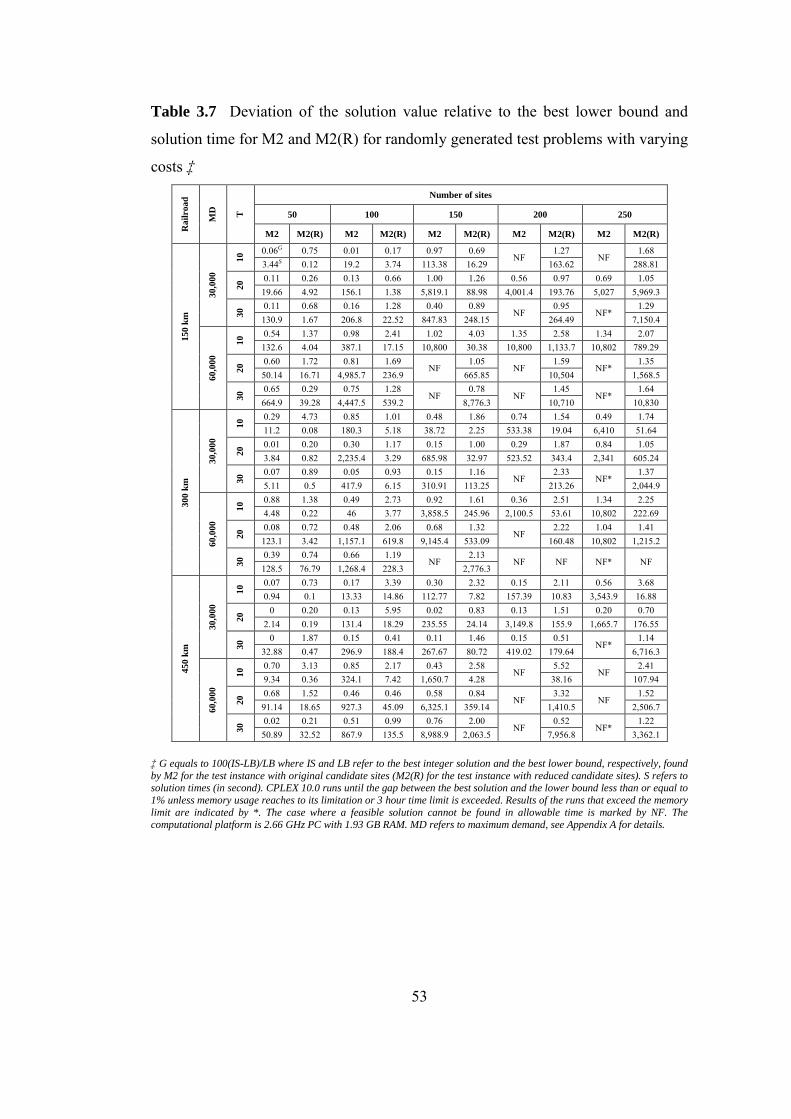
53

Table 3.7 Deviation of the solution value relative to the best lower bound and

solution time for M2 and M2(R) for randomly generated test problems with varying

costs ‡ R

ail

road

MD

T

Number of sites

50 100 150 200 250

M2 M2(R) M2 M2(R) M2 M2(R) M2 M2(R) M2 M2(R)

150 k

m

30,0

00

10

0.06G 0.75 0.01 0.17 0.97 0.69 NF

1.27 NF

1.68 3.44S 0.12 19.2 3.74 113.38 16.29 163.62 288.81

20

0.11 0.26 0.13 0.66 1.00 1.26 0.56 0.97 0.69 1.05 19.66 4.92 156.1 1.38 5,819.1 88.98 4,001.4 193.76 5,027 5,969.3

30 0.11 0.68 0.16 1.28 0.40 0.89

NF 0.95

NF* 1.29

130.9 1.67 206.8 22.52 847.83 248.15 264.49 7,150.4

60,0

00

10 0.54 1.37 0.98 2.41 1.02 4.03 1.35 2.58 1.34 2.07

132.6 4.04 387.1 17.15 10,800 30.38 10,800 1,133.7 10,802 789.29

20 0.60 1.72 0.81 1.69

NF 1.05

NF 1.59

NF* 1.35

50.14 16.71 4,985.7 236.9 665.85 10,504 1,568.5

30

0.65 0.29 0.75 1.28 NF

0.78 NF

1.45 NF*

1.64 664.9 39.28 4,447.5 539.2 8,776.3 10,710 10,830

30

0 k

m

30

,00

0

10 0.29 4.73 0.85 1.01 0.48 1.86 0.74 1.54 0.49 1.74

11.2 0.08 180.3 5.18 38.72 2.25 533.38 19.04 6,410 51.64

20

0.01 0.20 0.30 1.17 0.15 1.00 0.29 1.87 0.84 1.05 3.84 0.82 2,235.4 3.29 685.98 32.97 523.52 343.4 2,341 605.24

30 0.07 0.89 0.05 0.93 0.15 1.16

NF 2.33

NF* 1.37

5.11 0.5 417.9 6.15 310.91 113.25 213.26 2,044.9

60

,00

0

10 0.88 1.38 0.49 2.73 0.92 1.61 0.36 2.51 1.34 2.25

4.48 0.22 46 3.77 3,858.5 245.96 2,100.5 53.61 10,802 222.69

20

0.08 0.72 0.48 2.06 0.68 1.32 NF

2.22 1.04 1.41 123.1 3.42 1,157.1 619.8 9,145.4 533.09 160.48 10,802 1,215.2

30 0.39 0.74 0.66 1.19

NF 2.13

NF NF NF* NF 128.5 76.79 1,268.4 228.3 2,776.3

45

0 k

m

30

,00

0

10 0.07 0.73 0.17 3.39 0.30 2.32 0.15 2.11 0.56 3.68

0.94 0.1 13.33 14.86 112.77 7.82 157.39 10.83 3,543.9 16.88

20 0 0.20 0.13 5.95 0.02 0.83 0.13 1.51 0.20 0.70

2.14 0.19 131.4 18.29 235.55 24.14 3,149.8 155.9 1,665.7 176.55

30 0 1.87 0.15 0.41 0.11 1.46 0.15 0.51

NF* 1.14

32.88 0.47 296.9 188.4 267.67 80.72 419.02 179.64 6,716.3

60

,00

0

10

0.70 3.13 0.85 2.17 0.43 2.58 NF

5.52 NF

2.41 9.34 0.36 324.1 7.42 1,650.7 4.28 38.16 107.94

20

0.68 1.52 0.46 0.46 0.58 0.84 NF

3.32 NF

1.52 91.14 18.65 927.3 45.09 6,325.1 359.14 1,410.5 2,506.7

30 0.02 0.21 0.51 0.99 0.76 2.00

NF 0.52

NF* 1.22

50.89 32.52 867.9 135.5 8,988.9 2,063.5 7,956.8 3,362.1

‡ G equals to 100(IS-LB)/LB where IS and LB refer to the best integer solution and the best lower bound, respectively, found

by M2 for the test instance with original candidate sites (M2(R) for the test instance with reduced candidate sites). S refers to solution times (in second). CPLEX 10.0 runs until the gap between the best solution and the lower bound less than or equal to

1% unless memory usage reaches to its limitation or 3 hour time limit is exceeded. Results of the runs that exceed the memory

limit are indicated by *. The case where a feasible solution cannot be found in allowable time is marked by NF. The computational platform is 2.66 GHz PC with 1.93 GB RAM. MD refers to maximum demand, see Appendix A for details.

54

CHAPTER 4

THE DYNAMIC P-MEDIAN PROBLEM WITH MOBILE FACILITIES

In this chapter, a dynamic version of the p-median problem, which is motivated by

the problem considered in Chapter 3 is studied. The problem consists of dynamic

demands over the planning horizon and mobile facilities. Heuristic and exact

solution methods are proposed and their performances are evaluated by the

computational studies on the p-median problem instances taken from the literature

and randomly generated test problem instances.

4.1 Introduction

The dynamic demands and mobile facilities are two rich and distinctive properties

of the problem studied in Chapter 3. Being motivated by these properties, in this

chapter, we generalize this problem to the general networks under the p-median

problem settings, called the dynamic p-median problem (DPP) with mobile

facilities. There are dynamic demands over a planning horizon, T, and

predetermined numbers (p) of mobile and immobile facilities in each period of T.

According to some external considerations the number of facilities may decrease,

increase, or not change from one period to another period. If the predetermined

number of facilities from a type is fewer in a period compared to its previous

period, then some of these facilities are abolished in this period. If it is more, then

new facilities from that type must be opened. Abolishing and opening cannot be

realized simultaneously at a site. However, facility opening, moving, and abolishing

may occur many times at a location during the planning horizon. There are

relocation (moving) costs (fixed or source-and-sink dependent) for mobile facilities

and service (allocation) costs for customers. The problem is to determine the

55

opening-abolishing times and the locations of facilities, the movement times and

routes of mobile facilities, and the allocation of demands to open facilities in each

period such that the total cost is minimized.

Note that if the relocation costs are close to zero, then the DPP with mobile

facilities reduces to the T independent (classical) p-median problems (which will be

considered in detail in section 4.2.1). If the relocation costs are high, then it will not

be beneficial to relocate or to move the facilities anymore and the problem reduces

to the dynamic p-median problem (which will be studied in detail in Chapter 5).

4.2 Literature Review

4.2.1 Literature Review on the p-Median Problem

The Weber problem is to find p median points on a plane such that the total

distance between n weighted points and their nearest medians is minimized. Hakimi

(1964) considers a similar problem to the Weber problem in which one median is

restricted to the locations defined on a graph where there are a set of demand nodes

and a set of edges between the demand nodes. He shows that, in the optimal

solution, the median is located at a demand node. In other words, according to this

result, considering only nodes of the graph as candidate facility (median) locations

is enough to solve the problem to optimality. This property is called node

optimality property and makes the problem a discrete location problem. Hakimi

(1965) generalizes this problem to find p medians and proves that the node

optimality property is also valid for a more general problem, called “the p-median

problem”. Since we consider the dynamic p-median problem, below we review the

mathematical models developed for the p-median problem.

Mixed Integer Linear Programming Formulations

Let us consider a graph G=(N, E) where N is the set of demand nodes and E is the

set of edges between the demand nodes. Let P be the set of facilities, NP , wi be

56

a weight (demand) of node i, and dij be the minimum distance between nodes i and

j. It can be shown that a demand node satisfies its entire demand from the nearest

facility. It is an important result for the services provided by an uncapacitated

facility. The p-median problem is to find the locations of p facilities such that the

total weighted distance between the nodes and the nearest facilities is minimized,

i.e.,

Ni

ikPk

i

pPNP

dw }{minmin||

.

ReVelle and Swain (1970) present the following first integer-linear programming

formulation of the p-median problem.

Model 1 (ReVelle and Swain, 1970):

)4.4(,}1,0{

)3.4(

)2.4(

)1.4(1..

Njix

px

Njixx

Nix

ts

xdwMin

ij

Nj

jj

jjij

Nj

ij

Ni Nj

ijiji

In Model 1, binary decision variable xij is equal to 1 if demand node i is assigned to

a facility located at node j, and 0 otherwise. The objective is to minimize the total

weighted distance between the nodes and the facilities they are assigned to.

Constraint (4.1) forces each demand node to be assigned to a facility. Constraint

(4.2) guarantees to have a facility at node j if there is any demand node assigned to

this node. Constraint (4.3) sets the number of located facilities equal to p.

Constraint (4.2) is known as “Balinski” constraint since he was the first to write

such type constraints in 1965 when studying on the simple facility location

problem.

57

Garfinkel et al. (1974) show that it is not needed to define xij as binary variables for

i≠j in Model 1. Because facilities are uncapacitated and, as we discussed before,

each demand point automatically supplies its whole demand from the nearest open

facility. It follows that the assignment variables in Model 1 take only 0 or 1 value in

the optimal solution even their integrality constraint is relaxed. In order to prevent

fractional facility openings, however it is still needed to define location variables,

xjj, as binary variables. Authors also formulated the problem as a set partitioning

problem. The main observation is that the node subsets consisting of a median node

and the demand nodes assigned to that median node are disjoint subsets. In a

solution, N is partitioned into p such disjoint subsets. Notice that the cardinality of

such subsets can take a value between 1 and (n-p+1) where n is the cardinality of N.

The problem is to determine the p subsets of N such that each node in N belongs to

exactly one of the subsets and the total cost is minimized.

Let NSk , }{min

kk Si

ijiSj

k dwc and αik = 1 if node kSi , and 0 otherwise. Let m

be the number of node subsets. The binary decision variable xk is equal to 1 if Sk is

selected as one of p disjoint node subsets, and 0 otherwise. The set partitioning type

model of the p-median problem is then,

Model 2 (Garfinkel et al., 1974):

)7.4(,...,1}1,0{

)6.4(

)5.4(1

..

min

1

1

1

mkx

px

Nix

ts

xc

k

m

k

k

m

k

kik

m

k

kk

In Model 2, constraint (4.5) satisfies that each node belongs to exactly one subset

and constraint (4.6) forces to select exactly p subsets. So, the constraints

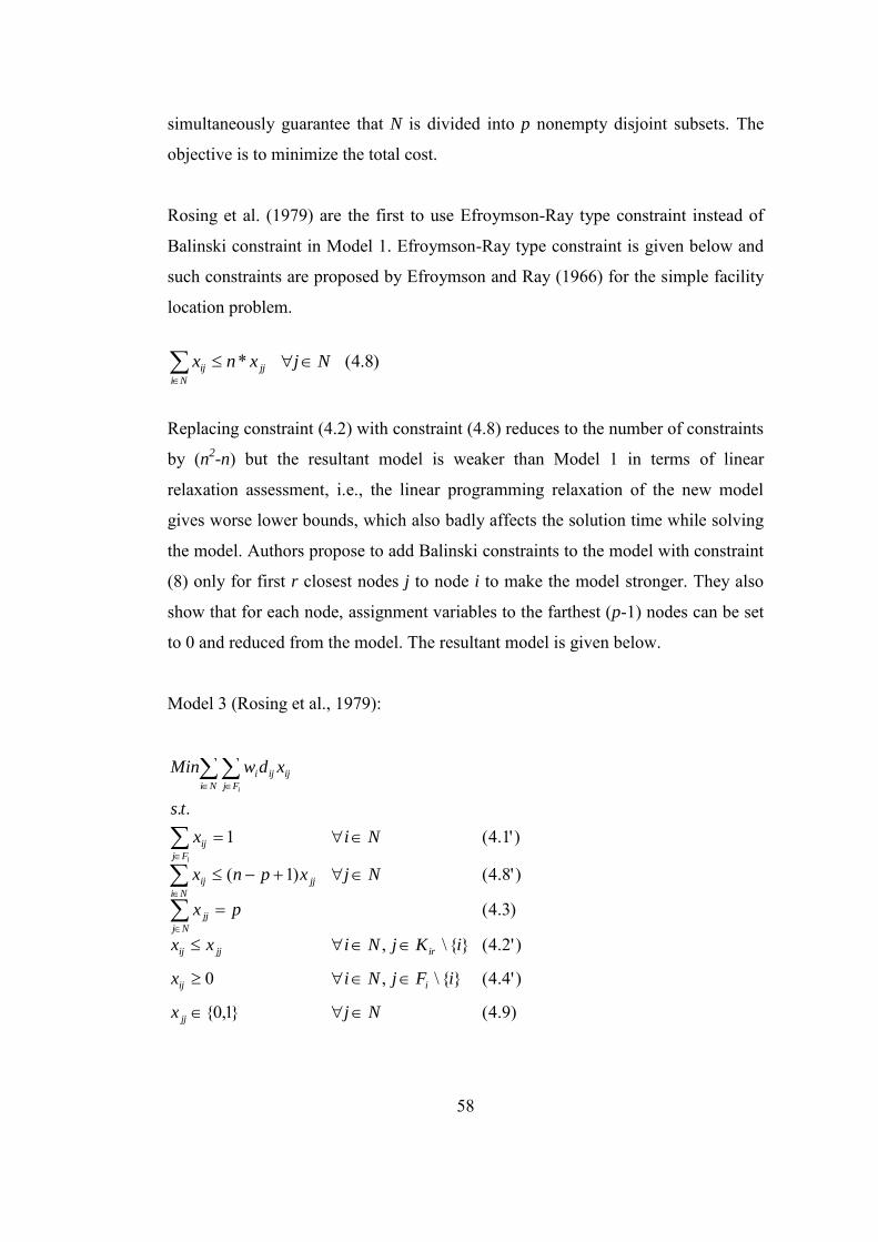
58

simultaneously guarantee that N is divided into p nonempty disjoint subsets. The

objective is to minimize the total cost.

Rosing et al. (1979) are the first to use Efroymson-Ray type constraint instead of

Balinski constraint in Model 1. Efroymson-Ray type constraint is given below and

such constraints are proposed by Efroymson and Ray (1966) for the simple facility

location problem.

)8.4(* Njxnx

Ni

jjij

Replacing constraint (4.2) with constraint (4.8) reduces to the number of constraints

by (n2-n) but the resultant model is weaker than Model 1 in terms of linear

relaxation assessment, i.e., the linear programming relaxation of the new model

gives worse lower bounds, which also badly affects the solution time while solving

the model. Authors propose to add Balinski constraints to the model with constraint

(8) only for first r closest nodes j to node i to make the model stronger. They also

show that for each node, assignment variables to the farthest (p-1) nodes can be set

to 0 and reduced from the model. The resultant model is given below.

Model 3 (Rosing et al., 1979):

)9.4(}1,0{

)'4.4(}{\,0

)'2.4(}{\,

)3.4(

)'8.4()1(

)'1.4(1..

Njx

iFjNix

iKjNixx

px

Njxpnx

Nix

ts

xdwMin

jj

iij

irjjij

Nj

jj

jj

Ni

ij

Fj

ij

Ni Fj

ijiji

i

i

59

In Model 3 Fi is the set of nodes except the (p-1) farthest nodes from node i and Kir

is the set of r-closest nodes to node i. In the objective function and constraints

(4.1’) and (4.4’), the decision variables between the nodes and the farthest (p-1)

nodes to each node is eliminated. Constraint (4.8) is tightened, using (n-p+1) as the

coefficient in the right hand side instead of n in (4.8’). Such a tightening is valid as

the number of nodes assigned to a median cannot exceed (n-p+1) because the

number of medians is set to p and each median is assigned to itself in the optimal

solution (also see explanation of Model 2).

Avella and Sassano (2001) present a new model using the fact that the assignment

of median nodes to themselves costs zero. The problem thus is to determine

remaining (n-p) assignment variables that take value 1. If a node is assigned to

another node, then no node can be assigned to this node because it is not a median

site. Similarly, if a node serves another node, then this node should be a median and

it cannot be assigned to another node. The new model is given below.

Model 4 (Avella and Sassano, 2001):

)12.4(}{\,}1,0{

)11.4(

)10.4(}{\,1..

min

}{\

}{\

}{\

iNjNix

pnx

iNkNixx

ts

xdw

ij

Ni iNj

ij

ki

iNj

ij

Ni iNj

ijiji

Note that xjj variables are reduced from the above model. But this time, if the

remaining variables (i.e., the variables used in Model 4) are not defined as binary,

then fractional facility openings can occur (i.e., it is not guaranteed that each

assignment variable takes value of 1 or 0 automatically in the optimal solution). So,

the assignment variables are defined as binary variables. In Model 4, constraint

(4.10) guarantees that if there is a node assigned to a node (say node i) than node i

cannot be assigned to another node, or if node i is assigned to another node than no

60

node can be assigned to node i. Constraint (4.11) guarantees that exactly (n-p)

assignment is made between different nodes.

Recently, Elloumi (2010) presents a new model, which is the adaptation of the

model developed for the uncapacitated facility location problem in Cornuejols et al.

(1980) and Cornuejols et al. (1990) to the p-median problem.

Let Gi be the number of different distances from node i. It follows that Gi ≤ |N|. Let iG

iii DDD ...21 be these distances, sorted in increasing order.

Model 5 (Elloumi, 2010):

)9.4(}1,0{

)15.4(,...,1,0

)14.4(0

)13.4(,...,1,1

)3.4(..

})({min1

1

11

Njx

GkNiz

Niz

GkNixz

px

ts

zDDwDw

jj

i

k

i

G

i

i

Dd

Nj

jj

k

i

Nj

jj

Ni

G

k

k

i

k

i

k

iiii

i

kiij

i

In Model 5 a new type decision variable, k

iz , is introduced. k

iz is equal to 1 if there

is no open facility at the nodes within the distance k

iD (distance k

iD is included)

from node i, and 0 otherwise. Constraint (4.13) ensure that for any node i, either at

least one facility is opened at the nodes within the distance k

iD or k

iz is equal to 1.

Although k

iz is defined as a binary variable, it is not needed to force it to be binary

in the model because it has a positive coefficient at the minimization type objective

function. This property, constraint (4.3) and constraint (4.9) all together guarantee

that k

iz is either 1 or 0 at the optimal solution.

61

Elloumi (2010) replaces constraint (4.13) with the following two constraints to do

the same work with constraint (4.13) and obtains an alternative model that has the

same linear programming value with Model 5.

)''13(,...,2,

)'13(1

1

1

1

i

k

i

Dd

Nj

jj

k

i

Dd

Nj

jji

KkNizxz

Nixz

kiij

iij

Garcia et al. (2011) use a modified version of Model 5. The main difference is that

this time distance k

iD is excluded in the definition of z variables.

Model 6 (Garcia et al. 2011): Radius Model

)15.4(,...,2,0

)9.4(}1,0{

)'''13.4(,...,2,1

)3.4(..

)(min2

1

i

k

i

jj

i

Dd

Nj

jj

k

i

Nj

jj

Ni

G

k

k

i

k

i

k

ii

GkNiz

Nix

GkNixz

px

ts

zDDw

kiij

i

In Model 6, the objective is to minimize the total allocation cost. Constraint

(4.13) does the same task with constraint (4.13) in Model 5. Figure 4.1 illustrates

how variables are used in Model 6 using an example.

Let’s consider the nodes i, a, b, c, d, and e on a graph, where

ieidicibiaii dddddd 0 . Assume that the nearest facility to node i be

located to node c, as shown in Figure 4.1. Note that in this solution

1...21 k

iii zzz and 0...21 iG

i

k

i

k

i zzz .

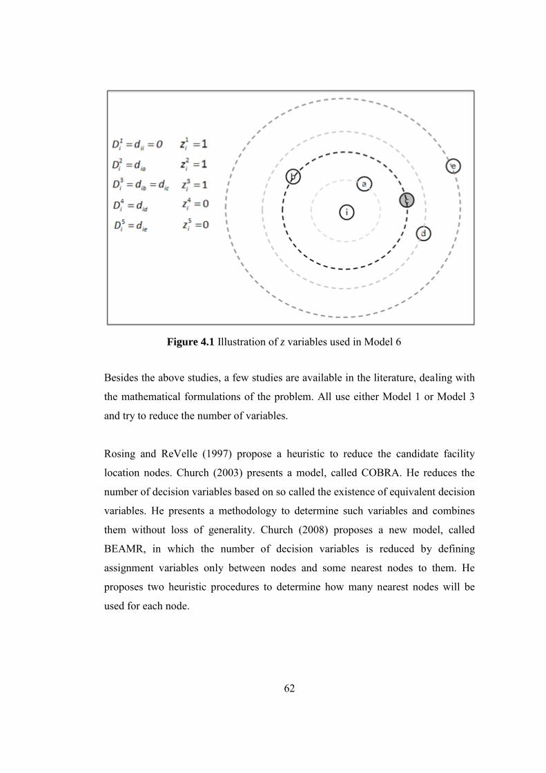
62

Besides the above studies, a few studies are available in the literature, dealing with

the mathematical formulations of the problem. All use either Model 1 or Model 3

and try to reduce the number of variables.

Rosing and ReVelle (1997) propose a heuristic to reduce the candidate facility

location nodes. Church (2003) presents a model, called COBRA. He reduces the

number of decision variables based on so called the existence of equivalent decision

variables. He presents a methodology to determine such variables and combines

them without loss of generality. Church (2008) proposes a new model, called

BEAMR, in which the number of decision variables is reduced by defining

assignment variables only between nodes and some nearest nodes to them. He

proposes two heuristic procedures to determine how many nearest nodes will be

used for each node.

Figure 4.1 Illustration of z variables used in Model 6

63

Exact Algorithms

Christofides and Beasley (1982) use a Lagrangian heuristic to obtain lower bounds.

These bounds and the heuristic procedure incorporated into a branch and bound

(BnB) algorithm. Beasley (1985) solves p-median problem instances with up to 900

nodes on a Cray supercomputer, using BnB.

Galvao (1980) develops a heuristic similar to the dual ascent algorithm, proposed

by Erlenkotter (1978) for the uncapacitated facility location problem, in order to

solve the dual of the LP relaxation of Model 1 and to obtain a lower bound. Galvao

solves the instances with up to 30 nodes faster than El-Shaieb (1973) and Jarvinen

et al. (1972).

There are several exact algorithms in the literature, using Lagrangian relaxation, LP

relaxation, and primal-dual relation in BnB algorithms (for example, see Cornuejols

et al. 1977; El-Shaieb 1973; Jarvinen et al. 1972; Narula et al. 1977; Revelle and

Swain 1970; Hanjoul and Peeters 1985; Mirchandani et al. 1985; Galvao and Raggi

1989). According to the best of our knowledge, several studies are carried out after

1989 but almost all of them offer heuristics.

Senne et al. (2005) present a branch and price algorithm that combines column

generation with Lagrangian relaxation in order to produce productive columns.

They solve the test instances taken from OR-Library, with up to 900 nodes. de

Farias (2001) proposes a branch and cut (BnC) algorithm while Elloumi and

Plateau (2010) and Garcia et al. (2011) propose a branch and price (BnP) algorithm

to solve Model 5.

Decomposition Methods

Garfinkel et al. (1974) use Dantzing-Wolfe decomposition to solve the LP

relaxation of Model 2 and combine group theory and dynamic programming (DP)

64

in order to handle the non-integer solutions. They solve test instances with up to 33

nodes.

Heuristics

Kariv and Hakimi (1979) prove that the p-median problem is NP-hard on a general

network for an arbitrary p. This result justifies many heuristic methods proposed in

the literature to find good solutions in reasonable times. Some selected heuristics

from Reese (2006) and Mladenovic et al. (2007), the most recent literature surveys,

are addressed below and the reader is referred to these surveys for the details of

heuristics listed.

Greedy heuristic (Kuehn and Hamburger 1963; Whitaker 1983), Stingy heuristic

(Feldman et al. 1966; Salhi and Atkinson 1995), dual-ascent heuristic (Galvao

1980; Galvao 1993; Captivo 1991), node substitution heuristic (Resende and

Werneck 2003), DP based heuristics (Hribar and Daskin 1997), Lagrangian

relaxation based heuristics (Beasley 1993), and node aggregation heuristics (Francis

et al. 2000). See also Reese (2006) and Mladenovic et al. (2007) for different meta-

heuristics such as genetic, tabu search, simulated annealing, variable neighborhood

search, heuristic concentration, scatter search, ant colony, neural networks, hybrids,

etc..

Avella et al. (2007) propose a complicated heuristic based on Lagrangian

relaxation, and branch and cut and price.

4.2.2 Literature Review on the Dynamic p-Median Problem

The p-median problems considered in the literature come with various extensions

such as with demand/distances uncertainty, multiple commodities/objectives,

capacities, etc.. Unfortunately, the dynamic version of the problem does not get a

lot attention in the literature.

65

Wesolowsky (1973) presents an integer formulation of the dynamic, continuous

single facility location problem and proposes a BnB based enumeration procedure

to solve it. The problem is to determine the locations of an uncapacitated mobile

facility on a plane at each discrete time period such that the total of customer

allocation and fixed facility relocation costs is minimized. Farahani et al. (2009)

study the dynamic, continuous single facility location problem with time dependent

customer weights. Facility relocations can occur at pre-determined time periods and

the objective is to minimize the total location and relocation cost. They present an

algorithm that first finds the optimal locations using constant weights and then finds

their relocation times.

Wesolowsky and Truscott (1975) fix the number of facilities to be run over the

planning horizon, limit the number of facility relocations in a period, and consider

fixed facility relocation costs for their dynamic p-median problem. They propose

two solution methods based on BnB and DP. Galvao and Santibanez-Gonzalez

(1992) study the problem in which the number of facilities to be open changes

according to a predetermined setting over the planning horizon. They propose a

Lagrangian heuristic to minimize the sum of allocation and facility installation

costs. Drezner (1995) considers p facilities to be located one by one over a p-period

planning horizon, called “the progressive p-median problem”. A heuristic method is

presented to minimize the allocation costs. These three studies and our study are

summarized in Table 4.1 for comparison purposes to highlight the similarities and

differences between the dynamic p-median problems that are studied in the

literature up to now.

According to Table 4.1, note that the present study is the only study considering

mobile and immobile facilities simultaneously and wholly relaxed relations

between the numbers of facilities to be open in sequential periods, and therefore, it

can be regarded as a generalization of the studies in the literature.

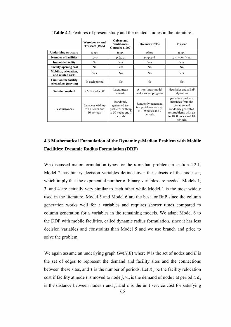
66

Table 4.1 Features of present study and the related studies in the literature.

Wesolowsky and

Truscott (1975)

Galvao and

Santibanez-

Gonzalez (1992) Drezner (1995) Present

Underlying structure graph graph plane graph Number of facilities pt=p pt ≥ pt-1 pt=pt-1+1 pt <, =, or > pt-1

Immobile facility No Yes Yes Yes Facility opening cost No Yes No No Mobility, relocation,

and related costs Yes No No Yes

Limit on the facility

relocations (moving) In each period No No No

Solution method a MIP and a DP Lagrangean heuristic

A non-linear model and a solver program

Heuristics and a BnP algorithm

Test instances

Instances with up to 10 nodes and

10 periods.

Randomly generated test

problems with up to 50 nodes and 7

periods.

Randomly generated test problems with up

to 100 nodes and 7 periods.

p-median problem instances from the

literature and randomly generated

test problems with up to 1000 nodes and 10

periods.

4.3 Mathematical Formulation of the Dynamic p-Median Problem with Mobile

Facilities: Dynamic Radius Formulation (DRF)

We discussed major formulation types for the p-median problem in section 4.2.1.

Model 2 has binary decision variables defined over the subsets of the node set,

which imply that the exponential number of binary variables are needed. Models 1,

3, and 4 are actually very similar to each other while Model 1 is the most widely

used in the literature. Model 5 and Model 6 are the best for BnP since the column

generation works well for z variables and requires shorter times compared to

column generation for x variables in the remaining models. We adapt Model 6 to

the DDP with mobile facilities, called dynamic radius formulation, since it has less

decision variables and constraints than Model 5 and we use branch and price to

solve the problem.

We again assume an underlying graph G=(N,E) where N is the set of nodes and E is

the set of edges to represent the demand and facility sites and the connections

between these sites, and T is the number of periods. Let Kij be the facility relocation

cost if facility at node i is moved to node j, wit is the demand of node i at period t, dij

is the distance between nodes i and j, and c is the unit service cost for satisfying

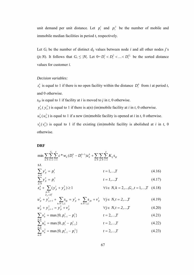
67

unit demand per unit distance. Let 1tp and 2

tp be the number of mobile and

immobile median facilities in period t, respectively.

Let Gi be the number of distinct dij values between node i and all other nodes j’s

(jN). It follows that Gi ≤ |N|. Let 0= iG

iii DDD ...21 be the sorted distance

values for customer i.

Decision variables: k

itz is equal to 1 if there is no open facility within the distance k

iD from i at period t,

and 0 otherwise.

sijt is equal to 1 if facility at i is moved to j in t, 0 otherwise. 1ity ( 2

ity ) is equal to 1 if there is a(n) (im)mobile facility at i in t, 0 otherwise.

1itu ( 2

itu ) is equal to 1 if a new (im)mobile facility is opened at i in t, 0 otherwise.

1itv ( 2

itv ) is equal to 1 if the existing (im)mobile facility is abolished at i in t, 0

otherwise.

DRF

)23.4(,...,2},0max{

)22.4(,...,2},0max{

)21.4(,...,2},0max{

)20.4(

)19.4(

)18.4(,...,1,21)(

)17.4(

)16.4(,...,1..

)(*min

221

2

11

11

111

1

2221,

2}/{

11

}/{

11,

1

21

22

11

22 1

1

Ttppv

Ttppu

Ttppv

T2,...,t N,jvyyu

T2,...,t N,jvsysyu

TtG,...,k N,iyyz

T1,...,tpy

Ttpy

ts

sKzDDwc

tt

Ni

it

tt

Ni

it

tt

Ni

it

jtjttjjt

jNi

jtjitjt

jNi

ijttjjt

i

Dd

Nj

jtjt

k

it

t

Nj

jt

t

Nj

jt

Ni Nj

T

t

ijtij

Ni

G

k

T

t

k

it

k

i

k

iit

kiji

i

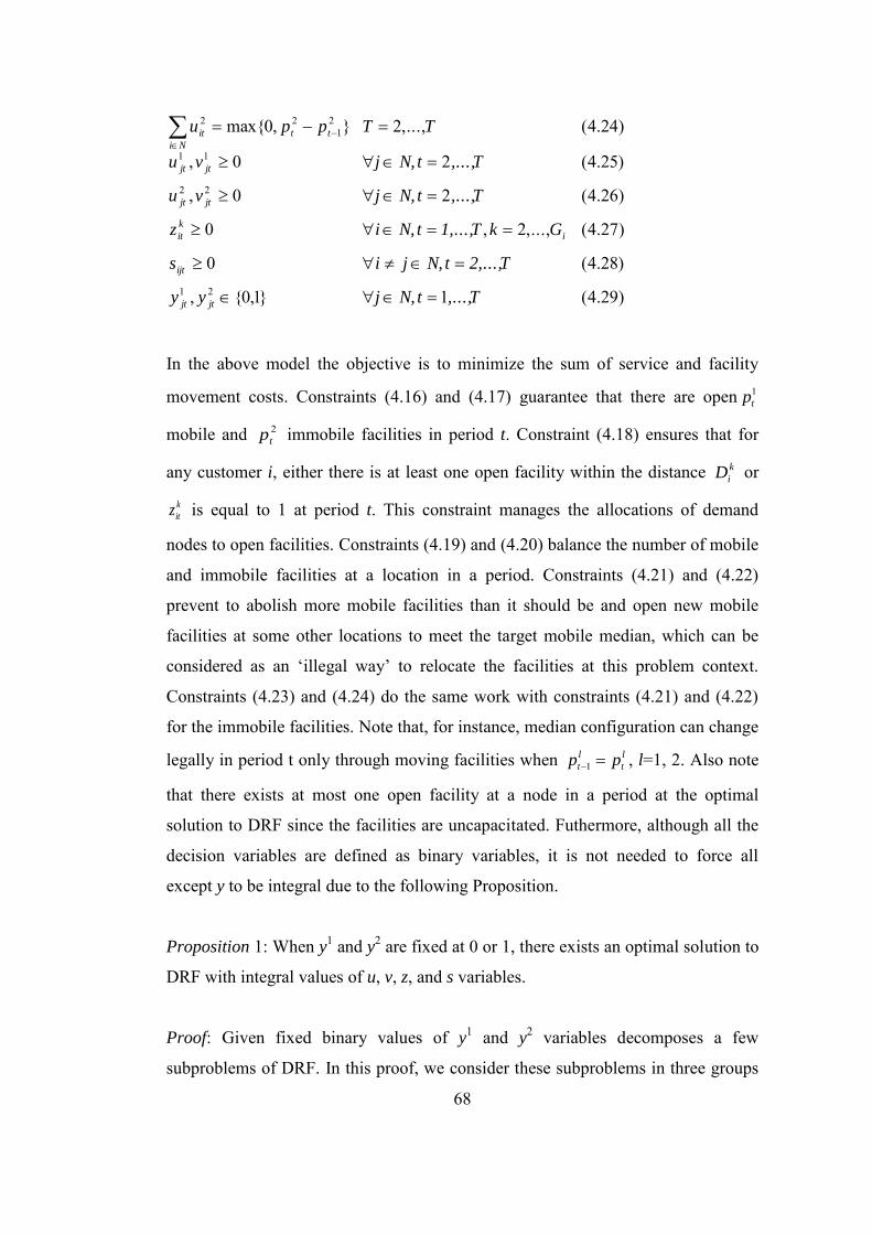
68

)29.4(1}1,0{,

)28.4(0

)27.4(,...,2,0

)26.4(20,

)25.4(20,

)24.4(,...,2},0max{

21

22

11

21

22

T,...,t N,jyy

T2,...,t N,jis

GkT1,...,t N,iz

T,...,t N,jvu

T,...,t N,jvu

TTppu

jtjt

ijt

i

k

it

jtjt

jtjt

tt

Ni

it

In the above model the objective is to minimize the sum of service and facility

movement costs. Constraints (4.16) and (4.17) guarantee that there are open 1tp

mobile and 2tp immobile facilities in period t. Constraint (4.18) ensures that for

any customer i, either there is at least one open facility within the distance k

iD or

k

itz is equal to 1 at period t. This constraint manages the allocations of demand

nodes to open facilities. Constraints (4.19) and (4.20) balance the number of mobile

and immobile facilities at a location in a period. Constraints (4.21) and (4.22)

prevent to abolish more mobile facilities than it should be and open new mobile

facilities at some other locations to meet the target mobile median, which can be

considered as an ‘illegal way’ to relocate the facilities at this problem context.

Constraints (4.23) and (4.24) do the same work with constraints (4.21) and (4.22)

for the immobile facilities. Note that, for instance, median configuration can change

legally in period t only through moving facilities when l

t

l

t pp 1 , l=1, 2. Also note

that there exists at most one open facility at a node in a period at the optimal

solution to DRF since the facilities are uncapacitated. Futhermore, although all the

decision variables are defined as binary variables, it is not needed to force all

except y to be integral due to the following Proposition.

Proposition 1: When y1 and y2 are fixed at 0 or 1, there exists an optimal solution to

DRF with integral values of u, v, z, and s variables.

Proof: Given fixed binary values of y1 and y

2 variables decomposes a few

subproblems of DRF. In this proof, we consider these subproblems in three groups

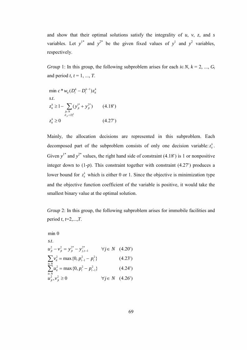
69

and show that their optimal solutions satisfy the integrality of u, v, z, and s

variables. Let y1* and y

2* be the given fixed values of y1 and y

2 variables,

respectively.

Group 1: In this group, the following subproblem arises for each iN, k = 2, ..., Gi

and period t, t = 1, ..., T.

)'27.4(0

)'18.4()(1..

)(*min

*2*1

1

k

it

Dd

Nj

jtjt

k

it

k

it

k

i

k

iit

z

yyz

ts

zDDwc

kiji

Mainly, the allocation decisions are represented in this subproblem. Each

decomposed part of the subproblem consists of only one decision variable: k

itz .

Given y1* and y2* values, the right hand side of constraint (4.18) is 1 or nonpositive

integer down to (1-p). This constraint together with constraint (4.27) produces a

lower bound for k

itz which is either 0 or 1. Since the objective is minimization type

and the objective function coefficient of the variable is positive, it would take the

smallest binary value at the optimal solution.

Group 2: In this group, the following subproblem arises for immobile facilities and

period t, t=2,...,T.

)'26.4(0,

)'24.4(},0max{

)'23.4(},0max{

)'20.4(..

0min

22

21

22

221

2

*21,

*222

Njvu

ppu

ppv

Njyyvu

ts

jtjt

tt

Ni

it

tt

Ni

it

tjjtjtjt

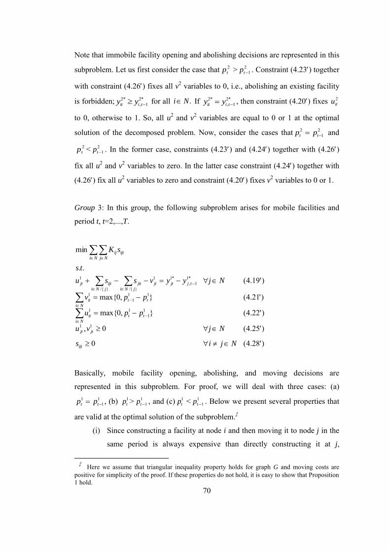
70

Note that immobile facility opening and abolishing decisions are represented in this

subproblem. Let us first consider the case that 2tp > 2

1tp . Constraint (4.23) together

with constraint (4.26) fixes all v2 variables to 0, i.e., abolishing an existing facility

is forbidden; *21,

*2 tiit yy for all .Ni If *2

1,*2

tiit yy , then constraint (4.20) fixes 2itu

to 0, otherwise to 1. So, all u2 and v2 variables are equal to 0 or 1 at the optimal

solution of the decomposed problem. Now, consider the cases that 21

2 tt pp and

2tp < 2

1tp . In the former case, constraints (4.23) and (4.24) together with (4.26)

fix all u2 and v2 variables to zero. In the latter case constraint (4.24) together with

(4.26) fix all u2 variables to zero and constraint (4.20) fixes v2 variables to 0 or 1.

Group 3: In this group, the following subproblem arises for mobile facilities and

period t, t=2,...,T.

)'28.4(0

)'25.4(0,

)'22.4(},0max{

)'21.4(},0max{

)'19.4(..

min

11

11

11

111

1

*11,

*1

}/{

1

}/{

1

Njis

Njvu

ppu

ppv

Njyyvssu

ts

sK

ijt

jtjt

tt

Ni

it

tt

Ni

it

tjjt

jNi

jtjit

jNi

ijtjt

Ni Nj

ijtij

Basically, mobile facility opening, abolishing, and moving decisions are

represented in this subproblem. For proof, we will deal with three cases: (a)1

11

tt pp , (b) 1tp > 1

1tp , and (c) 1tp < 1

1tp . Below we present several properties that

are valid at the optimal solution of the subproblem.‡ 1

(i) Since constructing a facility at node i and then moving it to node j in the

same period is always expensive than directly constructing it at j,

1 ‡ Here we assume that triangular inequality property holds for graph G and moving costs are

positive for simplicity of the proof. If these properties do not hold, it is easy to show that Proposition 1 hold.

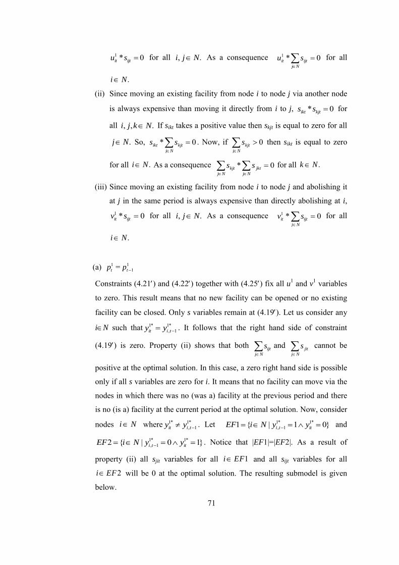
71

0*1 ijtit su for all ., Nji As a consequence 0*1 Nj

ijtit su for all

.Ni

(ii) Since moving an existing facility from node i to node j via another node

is always expensive than moving it directly from i to j, 0* kjtikt ss for

all .,, Nkji If sikt takes a positive value then skjt is equal to zero for all

.Nj So, 0* Nj

kjtikt ss . Now, if 0Nj

kjts then sikt is equal to zero

for all .Ni As a consequence 0* Nj

jkt

Nj

kjt ss for all .Nk

(iii) Since moving an existing facility from node i to node j and abolishing it

at j in the same period is always expensive than directly abolishing at i,

0*1 ijtit sv for all ., Nji As a consequence 0*1 Nj

ijtit sv for all

.Ni

(a) 1tp = 1

1tp

Constraints (4.21) and (4.22) together with (4.25) fix all u1 and v1 variables

to zero. This result means that no new facility can be opened or no existing

facility can be closed. Only s variables remain at (4.19). Let us consider any

iN such that *11,

*1 tiit yy . It follows that the right hand side of constraint

(4.19) is zero. Property (ii) shows that both Nj

ijts and Nj

jits cannot be

positive at the optimal solution. In this case, a zero right hand side is possible

only if all s variables are zero for i. It means that no facility can move via the

nodes in which there was no (was a) facility at the previous period and there

is no (is a) facility at the current period at the optimal solution. Now, consider

nodes Ni where *11,

*1 tiit yy . Let }01|{1 *1*1

1, itti yyNiEF and

}10|{2 *1*11, itti yyNiEF . Notice that |EF1|=|EF2|. As a result of

property (ii) all sjit variables for all 1EFi and all sijt variables for all

2EFi will be 0 at the optimal solution. The resulting submodel is given

below.

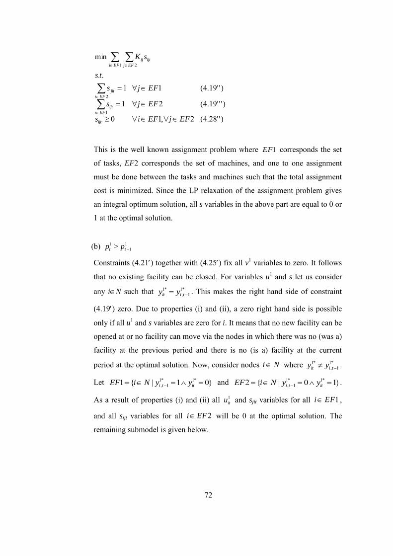
72

)''28.4(2,10

)'''19.4(21

)''19.4(11..

min

1

2

1 2

EFjEFis

EFjs

EFjs

ts

sK

ijt

EFi

ijt

EFi

jit

EFi EFj

ijtij

This is the well known assignment problem where 1EF corresponds the set

of tasks, EF2 corresponds the set of machines, and one to one assignment

must be done between the tasks and machines such that the total assignment

cost is minimized. Since the LP relaxation of the assignment problem gives

an integral optimum solution, all s variables in the above part are equal to 0 or

1 at the optimal solution.

(b) 1tp > 1

1tp

Constraints (4.21) together with (4.25) fix all v1 variables to zero. It follows

that no existing facility can be closed. For variables u1 and s let us consider

any iN such that *11,

*1 tiit yy . This makes the right hand side of constraint

(4.19) zero. Due to properties (i) and (ii), a zero right hand side is possible

only if all u1 and s variables are zero for i. It means that no new facility can be

opened at or no facility can move via the nodes in which there was no (was a)

facility at the previous period and there is no (is a) facility at the current

period at the optimal solution. Now, consider nodes Ni where *11,

*1 tiit yy .

Let }01|{1 *1*11, itti yyNiEF and }10|{2 *1*1

1, itti yyNiEF .

As a result of properties (i) and (ii) all 1itu and sjit variables for all 1EFi ,

and all sijt variables for all 2EFi will be 0 at the optimal solution. The

remaining submodel is given below.

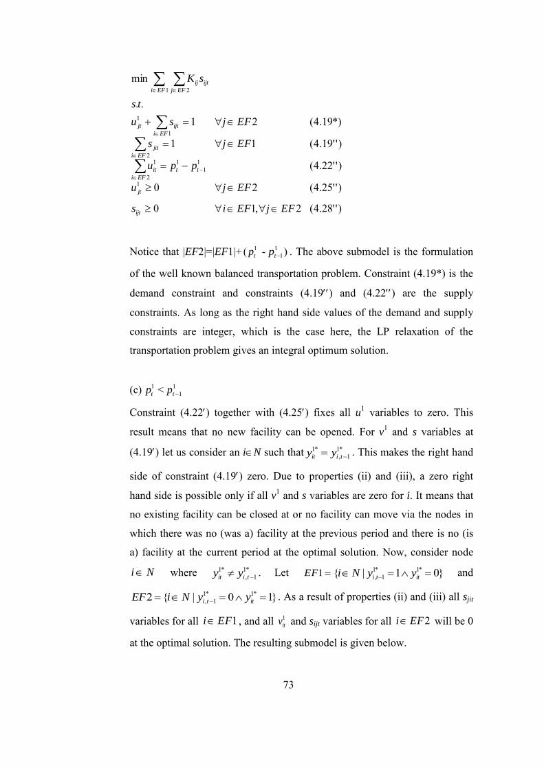
73

)''28.4(2,10

)''25.4(20

)''22.4(

)''19.4(11

*)19.4(21..

min

1

11

1

2

12

1

1

1 2

EFjEFis

EFju

ppu

EFjs

EFjsu

ts

sK

ijt

jt

tt

EFi

it

EFi

jit

EFi

ijtjt

EFi EFj

ijtij

Notice that |EF2|=|EF1|+ 1( tp - )11tp . The above submodel is the formulation

of the well known balanced transportation problem. Constraint (4.19*) is the

demand constraint and constraints (4.19) and (4.22) are the supply

constraints. As long as the right hand side values of the demand and supply

constraints are integer, which is the case here, the LP relaxation of the

transportation problem gives an integral optimum solution.

(c) 1tp < 1

1tp

Constraint (4.22) together with (4.25) fixes all u1 variables to zero. This

result means that no new facility can be opened. For v1 and s variables at

(4.19) let us consider an iN such that *11,

*1 tiit yy . This makes the right hand

side of constraint (4.19) zero. Due to properties (ii) and (iii), a zero right

hand side is possible only if all v1 and s variables are zero for i. It means that

no existing facility can be closed at or no facility can move via the nodes in

which there was no (was a) facility at the previous period and there is no (is

a) facility at the current period at the optimal solution. Now, consider node

Ni where *11,

*1 tiit yy . Let 1EF }01|{ *1*1

1, itti yyNi and

}10|{2 *1*11, itti yyNiEF . As a result of properties (ii) and (iii) all sjit

variables for all 1EFi , and all 1itv and sijt variables for all 2EFi will be 0

at the optimal solution. The resulting submodel is given below.

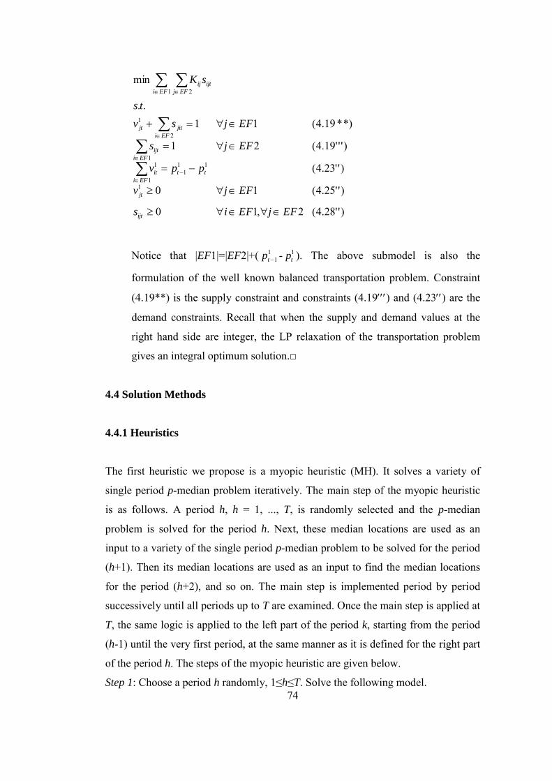
74

)''28.4(2,10

)''25.4(10

)''23.4(

)'''19.4(21

*)*19.4(11..

min

1

111

1

11

2

1

1 2

EFjEFis

EFjv

ppv

EFjs

EFjsv

ts

sK

ijt

jt

tt

EFi

it

EFi

ijt

EFi

jitjt

EFi EFj

ijtij

Notice that |EF1|=|EF2|+( 11tp - 1

tp ). The above submodel is also the

formulation of the well known balanced transportation problem. Constraint

(4.19**) is the supply constraint and constraints (4.19) and (4.23) are the

demand constraints. Recall that when the supply and demand values at the

right hand side are integer, the LP relaxation of the transportation problem

gives an integral optimum solution.□

4.4 Solution Methods

4.4.1 Heuristics

The first heuristic we propose is a myopic heuristic (MH). It solves a variety of

single period p-median problem iteratively. The main step of the myopic heuristic

is as follows. A period h, h = 1, ..., T, is randomly selected and the p-median

problem is solved for the period h. Next, these median locations are used as an

input to a variety of the single period p-median problem to be solved for the period

(h+1). Then its median locations are used as an input to find the median locations

for the period (h+2), and so on. The main step is implemented period by period

successively until all periods up to T are examined. Once the main step is applied at

T, the same logic is applied to the left part of the period k, starting from the period

(h-1) until the very first period, at the same manner as it is defined for the right part

of the period h. The steps of the myopic heuristic are given below.

Step 1: Choose a period h randomly, 1≤h≤T. Solve the following model.

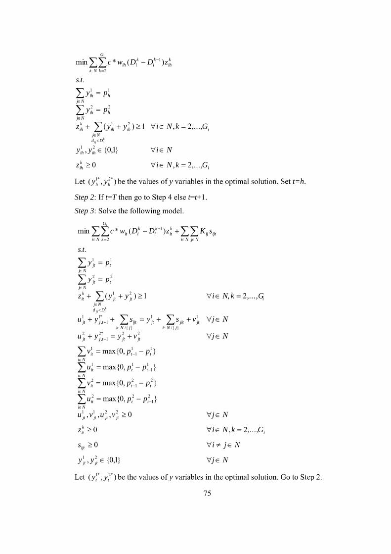
75

i

k

ih

ihih

i

Dd

Nj

ihih

k

ih

h

Nj

ih

h

Nj

ih

Ni

G

k

k

ih

k

i

k

iih

GkNiz

Niyy

GkNiyyz

py

py

ts

zDDwc

kiij

i

,...,2,0

}1,0{,

,...,2,1)(

..

)(*min

21

21

22

11

2

1

Let ),( *2*1hh yy be the values of y variables in the optimal solution. Set t=h.

Step 2: If t=T then go to Step 4 else t=t+1.

Step 3: Solve the following model.

Njyy

Njis

GkNiz

Njvuvu

ppu

ppv

ppu

ppv

Njvyyu

Njvsysyu

,...,Gk N,iyyz

py

py

ts

sKzDDwc

jtjt

ijt

i

k

it

jtjtjtjt

tt

Ni

it

tt

Ni

it

tt

Ni

it

tt

Ni

it

jtjttjjt

jNi

jtjitjt

jNi

ijttjjt

i

Dd

Nj

jtjt

k

it

t

Nj

jt

t

Nj

jt

Ni Nj

ijtij

Ni

G

k

k

it

k

i

k

iit

kiji

i

}1,0{,

0

,...,2,0

0,,,

},0max{

},0max{

},0max{

},0max{

21)(

..

)(*min

21

2211

21

22

221

2

11

11

111

1

22*21,

2}/{

11

}/{

*11,

1

21

22

11

2

1

Let ),( *2*1tt yy be the values of y variables in the optimal solution. Go to Step 2.

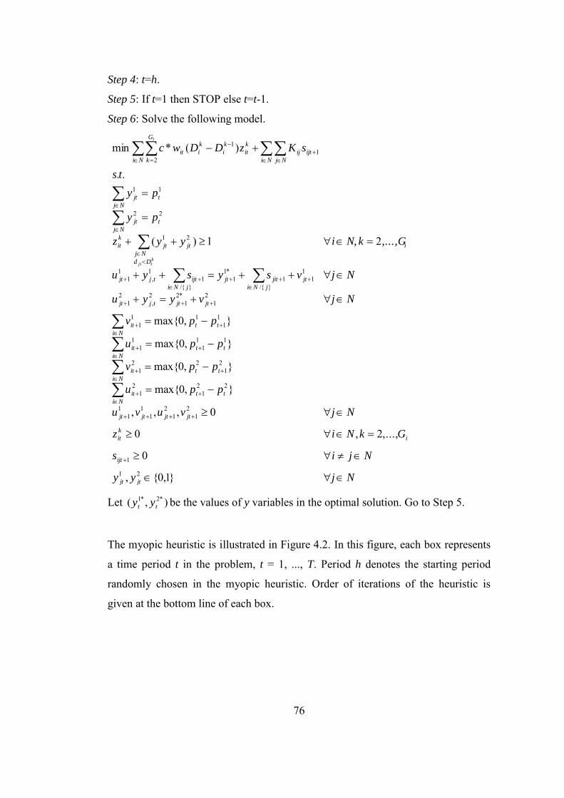
76

Step 4: t=h.

Step 5: If t=1 then STOP else t=t-1.

Step 6: Solve the following model.

Njyy

Njis

GkNiz

Njvuvu

ppu

ppv

ppu

ppv

Njvyyu

Njvsysyu

,...,Gk N,iyyz

py

py

ts

sKzDDwc

jtjt

ijt

i

k

it

jtjtjtjt

tt

Ni

it

tt

Ni

it

tt

Ni

it

tt

Ni

it

jtjttjjt

jNi

jtjitjt

jNi

ijttjjt

i

Dd

Nj

jtjt

k

it

t

Nj

jt

t

Nj

jt

Ni Nj

ijtij

Ni

G

k

k

it

k

i

k

iit

kiji

i

}1,0{,

0

,...,2,0

0,,,

},0max{

},0max{

},0max{

},0max{

21)(

..

)(*min

21

1

21

21

11

11

221

21

21

221

111

11

11

111

21

*21

2,

21

}/{

111

*11

}/{1

1,

11

21

22

11

12

1

Let ),( *2*1tt yy be the values of y variables in the optimal solution. Go to Step 5.

The myopic heuristic is illustrated in Figure 4.2. In this figure, each box represents

a time period t in the problem, t = 1, ..., T. Period h denotes the starting period

randomly chosen in the myopic heuristic. Order of iterations of the heuristic is

given at the bottom line of each box.

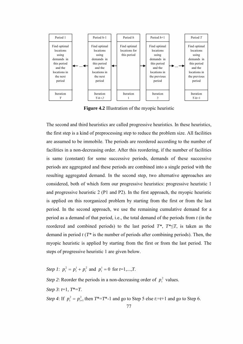
77

The second and third heuristics are called progressive heuristics. In these heuristics,

the first step is a kind of preprocessing step to reduce the problem size. All facilities

are assumed to be immobile. The periods are reordered according to the number of

facilities in a non-decreasing order. After this reordering, if the number of facilities

is same (constant) for some successive periods, demands of these successive

periods are aggregated and these periods are combined into a single period with the

resulting aggregated demand. In the second step, two alternative approaches are

considered, both of which form our progressive heuristics: progressive heuristic 1

and progressive heuristic 2 (P1 and P2). In the first approach, the myopic heuristic

is applied on this reorganized problem by starting from the first or from the last

period. In the second approach, we use the remaining cumulative demand for a

period as a demand of that period, i.e., the total demand of the periods from t (in the

reordered and combined periods) to the last period T*, T*≤T, is taken as the

demand in period t (T* is the number of periods after combining periods). Then, the

myopic heuristic is applied by starting from the first or from the last period. The

steps of progressive heuristic 1 are given below.

Step 1: 212ttt ppp and 01 tp for t=1,...,T.

Step 2: Reorder the periods in a non-decreasing order of 2tp values.

Step 3: t=1, T*=T.

Step 4: If 21

2 tt pp then T*=T*-1 and go to Step 5 else t:=t+1 and go to Step 6.

Period 1

Find optimal locations

using demands in this period

and the locations in

the next period

Iteration T

Period T

Find optimal locations

using demands in this period

and the locations in the previous

period

Iteration T-h+1

... ...

Figure 4.2 Illustration of the myopic heuristic

Period h-1

Find optimal locations

using demands in this period

and the locations in

the next period

Iteration T-h+2

Period h

Find optimal locations for this period

Iteration 1

Period h+1

Find optimal locations

using demands in this period

and the locations in the previous

period

Iteration 2

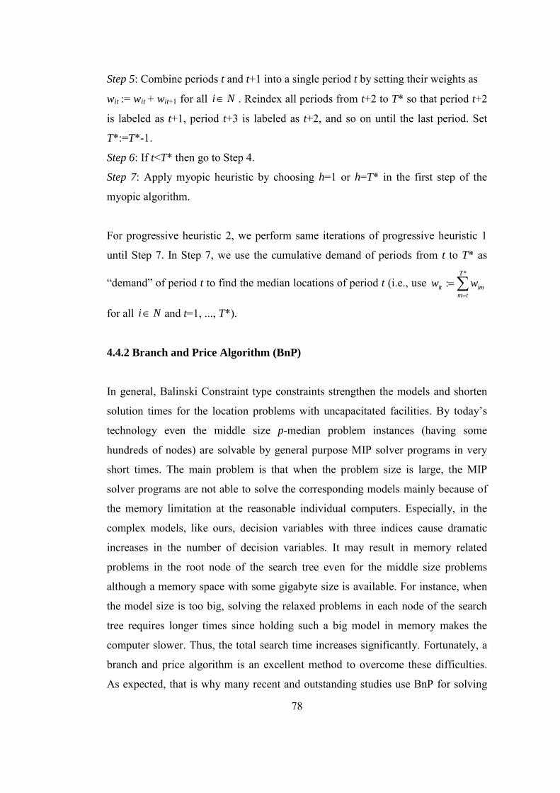
78

Step 5: Combine periods t and t+1 into a single period t by setting their weights as

wit := wit + wit+1 for all Ni . Reindex all periods from t+2 to T* so that period t+2

is labeled as t+1, period t+3 is labeled as t+2, and so on until the last period. Set

T*:=T*-1.

Step 6: If t<T* then go to Step 4.

Step 7: Apply myopic heuristic by choosing h=1 or h=T* in the first step of the

myopic algorithm.

For progressive heuristic 2, we perform same iterations of progressive heuristic 1

until Step 7. In Step 7, we use the cumulative demand of periods from t to T* as

“demand” of period t to find the median locations of period t (i.e., use

*

:T

tm

imit ww

for all Ni and t=1, ..., T*).

4.4.2 Branch and Price Algorithm (BnP)

In general, Balinski Constraint type constraints strengthen the models and shorten

solution times for the location problems with uncapacitated facilities. By today’s

technology even the middle size p-median problem instances (having some

hundreds of nodes) are solvable by general purpose MIP solver programs in very

short times. The main problem is that when the problem size is large, the MIP

solver programs are not able to solve the corresponding models mainly because of

the memory limitation at the reasonable individual computers. Especially, in the

complex models, like ours, decision variables with three indices cause dramatic

increases in the number of decision variables. It may result in memory related

problems in the root node of the search tree even for the middle size problems

although a memory space with some gigabyte size is available. For instance, when

the model size is too big, solving the relaxed problems in each node of the search

tree requires longer times since holding such a big model in memory makes the

computer slower. Thus, the total search time increases significantly. Fortunately, a

branch and price algorithm is an excellent method to overcome these difficulties.

As expected, that is why many recent and outstanding studies use BnP for solving

79

the p-median problem. Some of such studies are Avella et al. (2007), Garcia et al.

(2011), and Elloumi and Plateau (2010). This summarizes how we decided to

develop a branch and price algorithm as our solution procedure.

Column Generation and Branch and Price Algorithm

Column generation is a nice approach to deal with linear programming (LP) models

with a large number of decision variables. Assume that the LP solver is the simplex

algorithm. The main motivation of the method is that, if the basic decision variables

at the optimal solution were known, the reduction of the nonbasic variables at the

optimal solution from the LP model at the very beginning does not change the

optimal solution while providing significant savings in the total number of

operations. Here, the main difficulty is that the basic variables at the optimal

solution are not known at the beginning of the solution. Therefore, the main logic is

based on the fact that all decision variables are not needed in each iteration of the

solution algorithm. The search can be started with a subset of the decision variables

and, in each iteration of the algorithm, among the remaining variables only the ones

yielding improvement in the objective function value can be added to the subset of

the decision variables at the simplex table. Since the reduced costs of non basic

variables can be computed by using the values of dual variables, promising non

basic decision variables can be determined and the method continue to run in this

manner until finding the optimal LP solution.

When a mixed integer programming model is solved by a branch and bound

algorithm, in each node of the branch and bound (BnB) search tree, a linearly

relaxed model is solved. If the MIP model consists of too many decision variables,

solving these linear programming models in each node of the search tree may

necessitate enormous computational efforts. In order to overcome this matter, a

column generation method can be used in each node. The LP model in a node

initially consists of the decision variables that its parent node involves. For the root

node of the BnB tree, however, the initial subset of the entire decision variable set

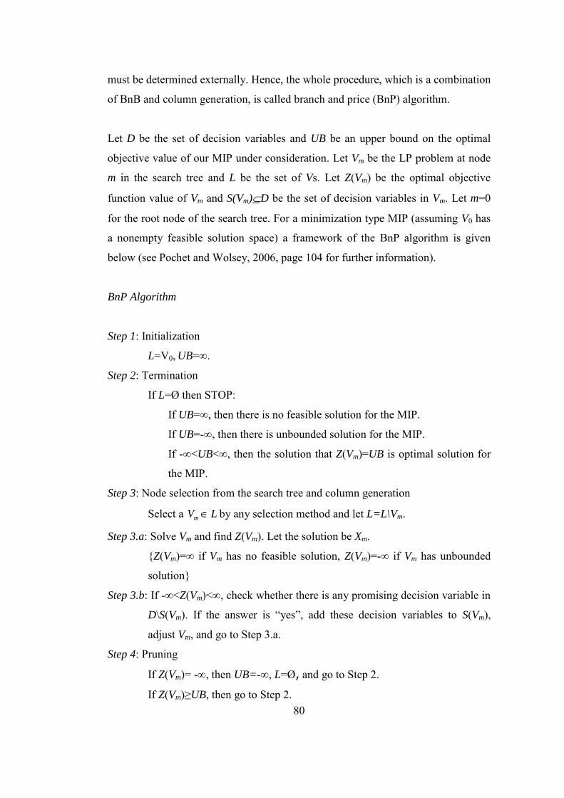
80

must be determined externally. Hence, the whole procedure, which is a combination

of BnB and column generation, is called branch and price (BnP) algorithm.

Let D be the set of decision variables and UB be an upper bound on the optimal

objective value of our MIP under consideration. Let Vm be the LP problem at node

m in the search tree and L be the set of Vs. Let Z(Vm) be the optimal objective

function value of Vm and S(Vm)D be the set of decision variables in Vm. Let m=0

for the root node of the search tree. For a minimization type MIP (assuming V0 has

a nonempty feasible solution space) a framework of the BnP algorithm is given

below (see Pochet and Wolsey, 2006, page 104 for further information).

BnP Algorithm

Step 1: Initialization

L=V0, UB=∞. Step 2: Termination

If L=Ø then STOP:

If UB=∞, then there is no feasible solution for the MIP.

If UB=-∞, then there is unbounded solution for the MIP.

If -∞<UB<∞, then the solution that Z(Vm)=UB is optimal solution for

the MIP.

Step 3: Node selection from the search tree and column generation

Select a LVm by any selection method and let L=L\Vm.

Step 3.a: Solve Vm and find Z(Vm). Let the solution be Xm.

{Z(Vm)=∞ if Vm has no feasible solution, Z(Vm)=-∞ if Vm has unbounded

solution}

Step 3.b: If -∞<Z(Vm)<∞, check whether there is any promising decision variable in

D\S(Vm). If the answer is “yes”, add these decision variables to S(Vm),

adjust Vm, and go to Step 3.a.

Step 4: Pruning

If Z(Vm)= -∞, then UB=-∞, L=Ø, and go to Step 2.

If Z(Vm)≥UB, then go to Step 2.

81

If -∞<Z(Vm)< UB and Xm satisfies integrality constraints in the MIP, then

UB=Z(Vm), L=L\{Vi: Z(Vi) ≥UB}, and go to Step 2.

Step 5: Branching

By branching generate new nodes from not pruned ones and L=L {the

new generated nodes}. Go to Step 2.

Note that Step 5 is performed after Step 4 when -∞<Z(Vm)< UB but Xm does not

satisfy integrality constraints in the MIP.

The skeleton of our solution procedure

The main reason of dramatic increases in the size of DRF is the three indices

decision variables, z and s. Thus, we start our BnP algorithm with subsets of these

decision variables and add the promising z and s variables, among the remaining

variables, one by one into the BnP algorithm. The initial S set is given below.

} ..., ,1 ,| ,{} ..., ,2 ,| , , ,{)( 212121

0 TtNiyyTtNivvuuVS itititititit

} ..., ,2 , ..., ,1 ,|{ it

k

it sdkTtNiz

Note that S(V0) contains no s variables and contains z variables for all nodes and

periods but only for k=2, ..., sdit, where sdit is any integer for node i and period t

between 2 and Gi and indicates the starting depth of z variables for node i and

period t. Determination of sdit values is explained later in this section.

In Step 3 of the BnP algorithm, we select node m according to depth first search

strategy. The number of the nodes on the path between node m and the root node of

the BnB tree shows the depth of node m. Note that each edge on this path means a

constraint on a variable, i.e., restriction on the branching variable. So, the deepest

node is the most restricted node. We select node m which is the one in the deepest

level in the search tree and having the branching variable fixed to its upper bound

(or lower bound). We use variable upper bound in our BnP algorithm. In Step 3.b,

we determine the promising z and s variables in D\S(Vm) and adjust Vm as follows.

82

Let S(Vm) include k

itz variables for TtNi ..., ,1 , , and k = 2, ..., rit, where

iitit Grsd . If itr

itz is positive in the optimal solution of Vm, then the next z

variable, 1itr

itz , is added to S(Vm). So, only checking the positive values of itr

itz variables at the optimal solution of Vm is enough to determine the variables that

must be added to Vm. This type of column generation fits the formulations like

Model 5 and Model 6 (Radius Formulation, see section 4.2.1). This method is a

generalization of the method used for the p-median problem in Garcia et al. (2011)

and Elloumi and Plateu (2010) to the dynamic p-median problems.

We should remind the reader that adjusting Vm implies not only adding a new

decision variable to the existing model of the problem but also adding a new

constraint to the existing model. Note that when 1itr

itz is added to the model, also

the following constraint, a member of constraint (4.18), is added to the model.

1)(1

211

itriji

it

Dd

Nj

jtjt

r

it yyz

On the other hand, we need dual variable values to determine the promising s

variables. Let βjt be a dual variable of constraint (4.19) for j and t. Note that s

variables are only used in constraint (4.19) and the objective function. Let us

consider two different nodes i and j and write the corresponding dual variables and

constraints belonging to (4.19) and for these nodes for a period t.

)()19.4(0}{}/{

11

}{}/{

11,

1it

ijNk

itijtiktitjit

ijNk

kittiit ivssyssyu

)()19.4(0}{}/{

11

}{}/{

11,

1jt

ijNk

jtjitjktjtijt

ijNk

kjttjjt jvssyssyu

Now, let us write the dual constraint for variable sjit.

83

jijtit K )(

So, if jijtit K )( , then the dual constraint for the decision variable sjit is

violated. In this case decision variable sjit is added to S(Vm).

In Step 5 of the above algorithm, we choose our branching variable from the

fractional valued y1 and y2 variables. We choose the variable whose value is closest

to a predetermined target value, which is one of the values 0.7, 0.8, and 0.9. We

calculate the absolute differences between values of fractional valued y1 and y

2

variables and the target value, and choose the variable having the minimum

difference. The flow chart of our BnP algorithm and explanations about how it

works are given in Appendix B.

From now on, we call our algorithm as the dynamic branch and price algorithm,

denoted by DBnP, specifically designed to solve the dynamic p-median problem

with mobile facilities.

Initialization for DBnP

Before starting to solve the DRF by DBnP, we need to solve the problem with one

of our heuristics to find an upper bound on the objective value of the dynamic p-

median problem. Recall that, in our heuristics, we solve the p-median like problems

for individual periods. We solve each of these problems by our BnP algorithm as

well. Since we do not have any particular idea about the promising starting depth

values (sdits) and not want to start the algorithm with undesirable z variables, we fix

all sdit parameters to 2 (i.e., k=2). Thus we start with only the first z variables for

each node and period, which indicates the closest node for each node.

Note that, after solving the problem with our heuristics, we have a solution at our

hand for the DRF and it provides some useful information to us for shortening the

solution time of DRF. Let Xh be the solution found by the heuristic and Z(Xh) be the

objective function value of this solution. While solving the DRF, in Step 1 of the

84

BnP algorithm we naturally use UB=Z(Xh) instead of UB=∞ in order to start with a

better upper bound to shorten the solution time. Furthermore, we determine the

starting depths for z variables using Xh in order not to start with a too small subset

of z variables that cause long solution times. Let k

ithXz )( be the value of k

itz at the

solution Xh. Here we determine the starting depth for node i and period t by the

expression: }0)(|)({minarg k

ith

k

ithk

it XzXzsd .

4.5 Computational Results

Test problem Instances

Our computational experiments are mainly performed to assess the performances of

the dynamic branch and price algorithm DBnP and the heuristics, myopic heuristic

MH and progressive heuristics P1 and P2, in solving relatively large practical

dynamic p-median problems with mobile facilities. Our computational experiments

are based on the test instances taken from the literature to generate dynamic

problem test instances. We use two platforms during our computations: (1) a 3.10

GHz PC with 6 GB RAM, (2) a 2.66 GHz PC with 1.93 GB RAM. In all

computations CPLEX 12.3 solver program is used as an LP solver and our

heuristics and DBnP algorithm are coded with C++ programming language.

We perform our computations on two groups of test problem instances: (1)

benchmarking p-median problem instances from the literature, (2) randomly

generated dynamic p-median problem instances. The instances in the second group

partitioned into two disjoint subsets, A and B, which will be explained later.

The first group of our test problem instances consists of 27 benchmarking p-median

problem instances with 900 nodes from the literature. The networks of the pmed38,

pmed39, and pmed40 test instances are used to generate the underlying structure of

these test instances. In total, 27 p-median problem instances are defined on these

85

networks with different p values and they are also tested in Avella et. al (2007) and

Garcia et al. (2011).

The second group consists of 160 randomly generated dynamic p-median problem

instances. In order to generate dynamic p-median test problem instances we use the

network and demand distribution of the following single period test problem

instances taken from the location literature:

SJC1 (100 demand and candidate facility location nodes), SJC2 (200

demand and candidate facility location nodes), SJC3 (300 demand and

candidate facility location nodes), and SJC4 (402 demand and candidate

facility location nodes) from the capacitated p-median problem literature

(http://www.lac.inpe.br/~lorena/instancias.html),

CAPA (1000 demand nodes, 100 candidate facility location nodes), CAPB

(1000 demand nodes, 100 candidate facility location nodes), and CAPC

(1000 demand nodes, 100 candidate facility location nodes) from the

capacitated warehouse location problem literature

(http://people.brunel.ac.uk/~mastjjb/jeb/info.html),

Australian Post (AP) data from the hub location problem literature

(original name of the problem is phub1) where the total amount of material

sent from a node to other nodes is taken as its demand (200 demand and

candidate facility location nodes

(http://people.brunel.ac.uk/~mastjjb/jeb/info.html).

These eight single period problem instances are converted to the dynamic problem

instances by using the method in Contrares et al. (2011). The obvious reason of

using single period test problem instances is the absence of dynamic test problem

instances in the literature.

Let N be the node set and di be the demand of node i in the (static) problem

instance. According to Contrares et. al. (2011), first a subset of N is randomly

chosen for the first period. Their demands are set to their original demands, dis. The

demands of remaining nodes in the first period are set to zero. Then, a subset of

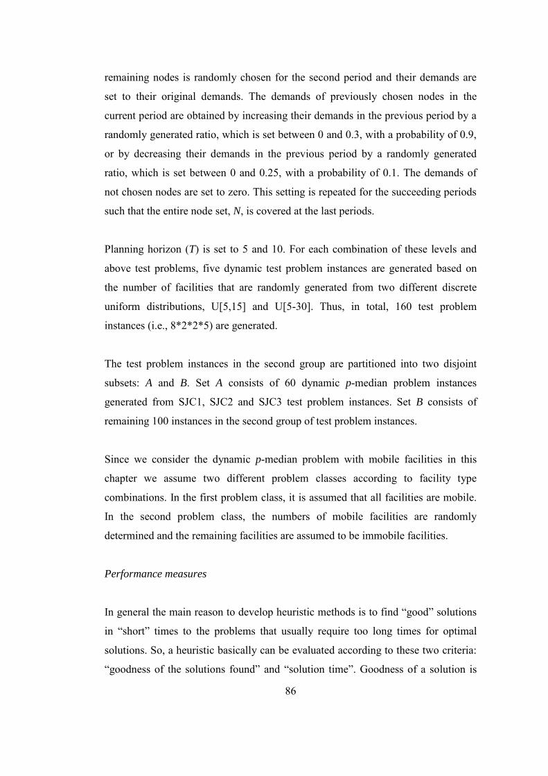
86

remaining nodes is randomly chosen for the second period and their demands are

set to their original demands. The demands of previously chosen nodes in the

current period are obtained by increasing their demands in the previous period by a

randomly generated ratio, which is set between 0 and 0.3, with a probability of 0.9,

or by decreasing their demands in the previous period by a randomly generated

ratio, which is set between 0 and 0.25, with a probability of 0.1. The demands of

not chosen nodes are set to zero. This setting is repeated for the succeeding periods

such that the entire node set, N, is covered at the last periods.

Planning horizon (T) is set to 5 and 10. For each combination of these levels and

above test problems, five dynamic test problem instances are generated based on

the number of facilities that are randomly generated from two different discrete

uniform distributions, U[5,15] and U[5-30]. Thus, in total, 160 test problem

instances (i.e., 8*2*2*5) are generated.

The test problem instances in the second group are partitioned into two disjoint

subsets: A and B. Set A consists of 60 dynamic p-median problem instances

generated from SJC1, SJC2 and SJC3 test problem instances. Set B consists of

remaining 100 instances in the second group of test problem instances.

Since we consider the dynamic p-median problem with mobile facilities in this

chapter we assume two different problem classes according to facility type

combinations. In the first problem class, it is assumed that all facilities are mobile.

In the second problem class, the numbers of mobile facilities are randomly

determined and the remaining facilities are assumed to be immobile facilities.

Performance measures

In general the main reason to develop heuristic methods is to find “good” solutions

in “short” times to the problems that usually require too long times for optimal

solutions. So, a heuristic basically can be evaluated according to these two criteria:

“goodness of the solutions found” and “solution time”. Goodness of a solution is

87

measured by the objective function. Since direct use of the objective function

values of heuristic solutions can be misleading, they are scaled by finding their

relative deviations from the lower bound (for minimization type problems) or

optimal values. So, the relative gaps between the objective function values of

heuristic solutions and lower bounds are used to measure the performances of

heuristic methods for goodness criterion.

For the exact solution methods the main performance evaluation criterion is the

solution time. But if a time limit is applied on solution time optimal solutions

would not be found in that limited time. In such a case some other criteria like

relative gaps between the best solutions found and lower bound values (for

minimization type problems), number of instances solved optimally in the limited

time, etc. may be used to evaluate the performances of the exact solution methods.

In this study we use the above criteria to evaluate the performances of our heuristics

and DBnP algorithm.

Our computational studies consist of three parts: (i) validation of DBnP, (ii)

deciding on parameter setting for the algorithm on a subset of our dynamic test

problem instances, and (iii) assessments of our algorithm’s performance on a larger

set of dynamic test problem instances.

4.5.1 Validation of DBnP

Before dealing with the dynamic problems, we first solve the (single period) p-

median test problem instances in the first group in order to validate our algorithm.

Although these computations are mainly for validation purpose, the solution times

also show that our algorithm competes with Avella et al. (2007) and Garcia et al.

(2011), which are two benchmarking studies for us. Solution times are given in

Table 4.2.

Since there are many factors affecting the computational performances such as

running programs, type-model of the RAM components, processor type-model,

88

version of the used solver programs, etc., it is hard to make certain comparisons.

Roughly speaking, our computer, the first one, is 1.7 times faster than the one in

Avella et al. (2007) and 1.3 times faster than the one in Garcia et al. (2011)

according to the number of operations done in a second. Therefore, in Table 4.2,

adjusted results are given. According to overall results, we solved 26 of 27

instances faster than Avella et al. (2007) and 18 of 27 instances faster than Garcia et

al. (2011). On the other hand, average solution times are 40 seconds for Avella et

al. (2007), 6.13 seconds for Garcia et al. (2007) and 19.2 seconds for the current

study. So, on average Garcia et al. (2011) is the best.

Table 4.2 Solution times (sec.) for the p-median problem test instances in the first

group†

Instance Avella et al.

(2007) Garcia et al.

(2011) DBnP

Pmed38-5 188.24 23.08 81 Pmed38-10 236.47 20.77 136 Pmed38-20 24.12 6.92 8 Pmed38-50 18.82 3.85 1

Pmed38-100 4.71 1.54 0.01 Pmed38-200 4.71 2.31 0.01 Pmed38-300 4.71 2.31 0.01 Pmed38-400 4.12 2.31 0.01 Pmed38-500 4.12 2.31 0.01 Pmed39-5 104.12 21.54 57 Pmed39-10 159.41 15.38 59 Pmed39-20 10.00 2.31 2 Pmed39-50 21.76 4.62 4

Pmed39-100 4.71 3.08 0.01 Pmed39-200 4.71 2.31 0.01 Pmed39-300 4.12 2.31 0.01 Pmed39-400 4.12 2.31 0.01 Pmed39-500 4.12 2.31 0.01 Pmed40-5 72.94 10.77 16 Pmed40-10 94.12 10.77 36 Pmed40-20 42.35 5.38 9 Pmed40-50 38.82 6.15 126 Pmed40-90 5.29 1.54 0.01

Pmed40-200 4.71 2.31 0.01 Pmed40-300 4.71 2.31 0.01 Pmed40-400 5.29 2.31 0.01 Pmed40-500 4.71 2.31 0.01

† Our computer is roughly 1.7 and 1.3 times faster compared to Avella et al. (2007) and Garcia et

al. (2011), respectively, according to the number of the operations done per second. Therefore, the

solution times for benchmarking studies are adjusted accordingly.

89

4.5.2 Experiments on the First Problem Class Involving Only Mobile

Facilities

In this section all facilities are assumed to be mobile. Computations in this part are

performed on a 2.66 GHz PC with 1.93 GB RAM, i.e., the second computer.

A. Testing Performances of Heuristics and Parameter Setting

We use test instances in set A of the second group to evaluate the performances of

heuristics and to determine the target value for DBnP procedure. We choose period

1, period 3 and period 5 as the starting period h for myopic heuristic MH for the

instances with five periods. We choose period 1, period 4, period 7 and period 10 as

the starting period h for the instances with ten periods. For our progressive

heuristics P1 and P2, we start with the first and last periods of the reordered and

combined periods of the original problem instances.

Average solution times and average relative gaps between the upper bounds (UB)

obtained by the heuristics and the lower bounds obtained by the linear

programming relaxations (LPR) of the models are given in Table 4.3. The reason of

using the LPR values in these experiments is the absence of the optimal solutions

yet. In order to measure the performances we solve the LP relaxations in this

experiment. Note that each row in Table 4.3 displays average values of 30 test

problem instances.

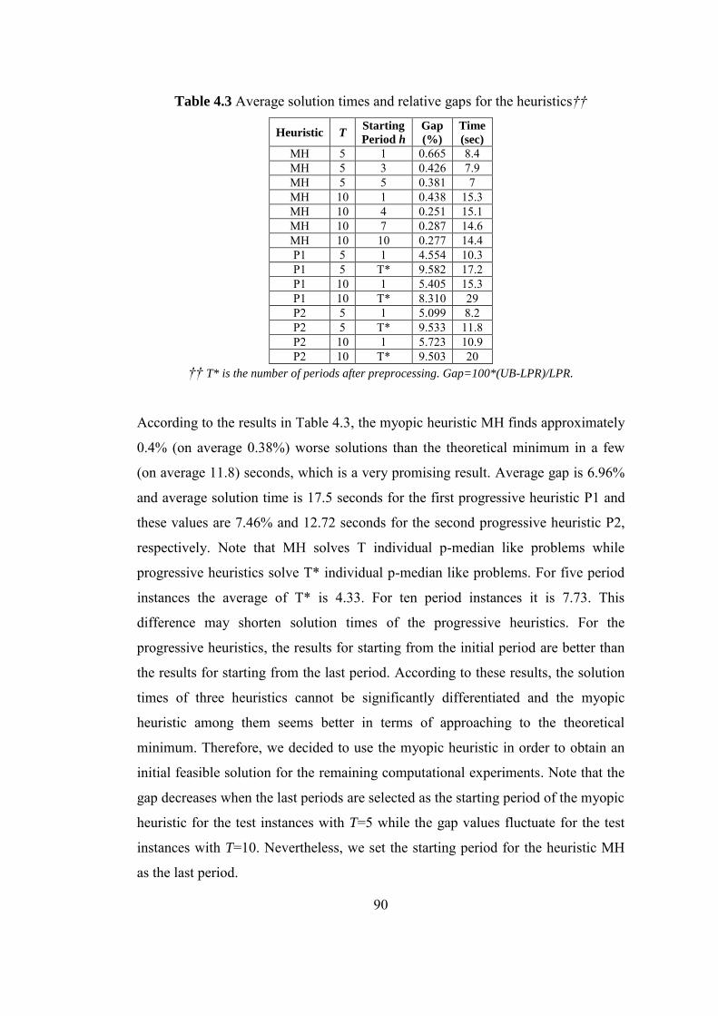
90

Table 4.3 Average solution times and relative gaps for the heuristics††

Heuristic T Starting

Period h

Gap

(%)

Time

(sec)

MH 5 1 0.665 8.4 MH 5 3 0.426 7.9 MH 5 5 0.381 7 MH 10 1 0.438 15.3 MH 10 4 0.251 15.1 MH 10 7 0.287 14.6 MH 10 10 0.277 14.4 P1 5 1 4.554 10.3 P1 5 T* 9.582 17.2 P1 10 1 5.405 15.3 P1 10 T* 8.310 29 P2 5 1 5.099 8.2 P2 5 T* 9.533 11.8 P2 10 1 5.723 10.9 P2 10 T* 9.503 20

†† T* is the number of periods after preprocessing. Gap=100*(UB-LPR)/LPR.

According to the results in Table 4.3, the myopic heuristic MH finds approximately

0.4% (on average 0.38%) worse solutions than the theoretical minimum in a few

(on average 11.8) seconds, which is a very promising result. Average gap is 6.96%

and average solution time is 17.5 seconds for the first progressive heuristic P1 and

these values are 7.46% and 12.72 seconds for the second progressive heuristic P2,

respectively. Note that MH solves T individual p-median like problems while

progressive heuristics solve T* individual p-median like problems. For five period

instances the average of T* is 4.33. For ten period instances it is 7.73. This

difference may shorten solution times of the progressive heuristics. For the

progressive heuristics, the results for starting from the initial period are better than

the results for starting from the last period. According to these results, the solution

times of three heuristics cannot be significantly differentiated and the myopic

heuristic among them seems better in terms of approaching to the theoretical

minimum. Therefore, we decided to use the myopic heuristic in order to obtain an

initial feasible solution for the remaining computational experiments. Note that the

gap decreases when the last periods are selected as the starting period of the myopic

heuristic for the test instances with T=5 while the gap values fluctuate for the test

instances with T=10. Nevertheless, we set the starting period for the heuristic MH

as the last period.

91

Below our aim is to determine the best target value for DBnP and solve the

remaining instances with these settings and evaluate the performance of DBnP. We

solve the 60 test instances in set A of the second group by DBnP with target values

of 0.7, 0.8, and 0.9, where initial feasible solution is found by the MH starting with

the last period. We set 5 hour time limit (18,000 sec) on total computational time

for a test instance. All instances are solved at optimality when the target value is 0.7

and 0.8. Only one out of 60 instances was not solved at optimality with the target

value of 0.9. Average solution time is 138.8 seconds, 147.5 seconds, and 433.8

seconds for the target values of 0.7, 0.8, and 0.9, respectively. Average number of

nodes searched in the DBnP tree is 5.8, 6.7, and 10.8 for the target values of 0.7,

0.8, and 0.9, respectively. According to these results, the target value 0.7

outperforms the others in these experiments.

B. Testing performance of DBnP

In the last part of our computational experiment on the first problem class, we solve

test instances in set B of the second group plus the test instances in set A that are not

solved in 5 hour time limit in the previous experiments. We set 10 hour limit

(36,000 sec) to each run. Average results for the entire set of second group are

given in Table 4.4.

145 of 160 instances are solved optimally in 10 hours. The overall average relative

gap between the best solution and LPR values is 0.05%. The overall average total

solution time is 4890 seconds. The overall average relative gap between the

heuristic solution and LPR values is 0.24%. The overall average solution time is 51

seconds for the heuristic. The reason of using LPR values in performance

evaluating is the existence of unsolved instances. According to these results myopic

heuristic has a good performance. As expected total solution time increases as the

problem size (number of the nodes, length of the planning horizon) increases. Small

instances (instances having 100, 200 nodes) are solved in some seconds or few

minutes. 13 of the unsolved problems belong to instances having 1,000 nodes.

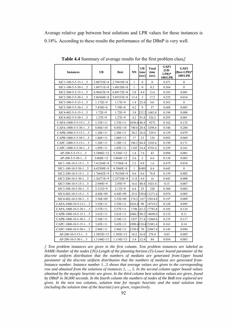
92

Average relative gap between best solutions and LPR values for these instances is

0.18%. According to these results the performance of the DBnP is very well.

Table 4.4 Summary of average results for the first problem class‡

Instances UB Best NN UB

tıme

(sec)

Total

time

(sec)

GAP1

(UB-

LPR)*

100/LPR

GAP2

(Best-LPR)*

100/LPR

SJC1-100-5-5-15-1…5 2.80735E+8 2.79419E+8 1 0 0 0.471 0 SJC1-100-5-5-30-1…5 1.60711E+8 1.60128E+8 1 0 0.2 0.364 0 SJC2-200-5-5-15-1…5 6.90432E+8 6.89172E+8 2.8 4.4 13.6 0.183 0.001 SJC2-200-5-5-30-1…5 5.86568E+8 5.85333E+8 13.4 3 17.2 0.225 0.014 SJC3-300-5-5-15-1…5 1.172E+9 1.17E+9 1.4 25.4 161 0.363 0 SJC3-300-5-5-30-1…5 7.438E+8 7.39E+8 4.2 9 37 0.688 0.003 SJC4-402-5-5-15-1…5 1.72E+9 1.72E+9 3.8 212.2 1683.8 0.194 0.008 SJC4-402-5-5-30-1…5 1.27E+9 1.27E+9 4.2 91.8 326.2 0.293 0.001

CAPA-1000-5-5-15-1…5 1.33E+11 1.33E+11 1036.6 48.4 9272 0.162 0.135 CAPA-1000-5-5-30-1…5 8.86E+10 8.85E+10 740.6 20.4 3298.4 0.346 0.204 CAPB-1000-5-5-15-1…5 1.28E+11 1.28E+11 30.2 26.6 229.4 0.129 0.079 CAPB-1000-5-5-30-1…5 1.06E+11 1.06E+11 17 23 124 0.092 0.069 CAPC-1000-5-5-15-1…5 1.28E+11 1.28E+11 196.2 44.4 2243.6 0.199 0.171 CAPC-1000-5-5-30-1…5 1.05E+11 1.05E+11 1103 34.4 8743.4 0.259 0.161

AP-200-5-5-15-1…5 5.3406E+12 5.336E+12 1.4 7.6 43 0.094 0.001 AP-200-5-5-30-1…5 3.068E+12 3.064E+12 2.6 2 6.6 0.138 0.003

SJC1-100-10-5-15-1…5 7.41264E+8 7.3786E+8 2.2 0.8 1.6 0.479 0.018

SJC1-100-10-5-30-1…5 4.42509E+8 4.3968E+8 1 0.001 0.4 0.642 0 SJC2-200-10-5-15-1…5 1.76642E+9 1.76356E+9 8.6 8.6 76.8 0.159 0.002 SJC2-200-10-5-30-1…5 1.26271E+9 1.25724E+9 11.8 4.4 16 0.443 0.008 SJC3-300-10-5-15-1…5 2.949E+9 2.95E+9 16.6 48.4 1021.6 0.15 0.007 SJC3-300-10-5-30-1…5 2.121E+9 2.11E+9 6.4 25 320 0.304 0.003 SJC4-402-10-5-15-1…5 4.44E+09 4.44E+09 25.6 330.6 11271.6 0.074 0.005 SJC4-402-10-5-30-1…5 3.36E+09 3.35E+09 174.2 167 15014.4 0.197 0.009

CAPA-1000-10-5-15-1…5 3.55E+11 3.55E+11 1016.8 98 14719.2 0.128 0.095 CAPA-1000-10-5-30-1…5 2.57E+11 2.57E+11 1796 63.2 17783.8 0.185 0.134 CAPB-1000-10-5-15-1…5 3.61E+11 3.61E+11 1066.2 90.2 14698.6 0.133 0.11 CAPB-1000-10-5-30-1…5 2.54E+11 2.54E+11 1037 37.4 11060.6 0.155 0.117 CAPC-1000-10-5-15-1…5 3.65E+11 3.65E+11 1098.6 110.4 21881.4 0.161 0.14 CAPC-1000-10-5-30-1…5 2.96E+11 2.96E+11 1358.8 70 22067.4 0.145 0.094

AP-200-10-5-15-1…5 1.3852E+13 1.385E+13 10.2 16.8 276.4 0.03 0.005 AP-200-10-5-30-1…5 1.1144E+13 1.114E+13 3.4 12.4 84 0.054 0.003

‡ Test problem instances are given in the first column. Test problem instances are labeled as

NAME-Number of the nodes (|N|)-Length of the planning horizon (T)-Lower bound parameter of the

discrete uniform distribution that the numbers of medians are generated from-Upper bound

parameter of the discrete uniform distribution that the numbers of medians are generated from-

Instance number. Instance number 1...5 shows that average values are given in the corresponding

row and obtained from the solutions of instances 1, ..., 5. In the second column upper bound values

obtained by the myopic heuristic are given. In the third column best solution values are given, found

by DBnP in 36,000 seconds. In the fourth column the numbers of nodes of the BnB tree explored are

given. In the next two columns, solution time for myopic heuristic and the total solution time

(including the solution time of the heuristic) are given, respectively.

93

4.5.3 Experiments on the Second Problem Class Involving Mobile and

Immobile Facilities

In this section the numbers of mobile facilities are randomly determined and the

remaining facilities are assumed to be immobile facilities. Computations are

performed on our second computer.

A. Testing Performances of Heuristics and Parameter Setting

We use test instances in set A of the second group to evaluate the performances of

heuristics and to determine the target value for DBnP procedure. We choose period

1, period 3 and period 5 as the starting period h for myopic heuristic MH for the

instances with five periods. We choose period 1, period 4, period 7 and period 10 as

the starting period h for the instances with ten periods. For our progressive

heuristics P1 and P2, we start with the first and last periods of the reordered and

combined periods of the original problem instances.

The solution time was very high (approximately 75 minutes) for only one instance

while almost all the remaining solution times were under 100 seconds for the

myopic heuristic. For the same instance when the starting period is different the

time is about 3 seconds. Because we use depth first search if fractional solution

cause to select a wrong variable as branching variable it may completely change the

search direction and would cause such a situation. Since it is an extreme situation

we omitted this instance when we are deciding. The average solution times and the

average relative gaps between the upper bounds (UB) obtained by the heuristics and

the lower bounds obtained by the linear relaxations (LPR) of the models are given

in Table 4.5. The reason of using the LPR values in these experiments is the

absence of the optimal solutions yet. In order to measure the performances we solve

the LP relaxations in this experiment. Note that each row of the Table 4.5 displays

average values of 30 test problem instances.

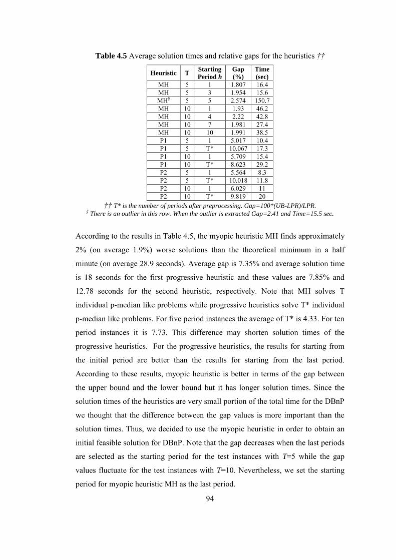
94

Table 4.5 Average solution times and relative gaps for the heuristics ††

Heuristic T Starting

Period h

Gap

(%)

Time

(sec)

MH 5 1 1.807 16.4 MH 5 3 1.954 15.6 MH§ 5 5 2.574 150.7 MH 10 1 1.93 46.2 MH 10 4 2.22 42.8 MH 10 7 1.981 27.4 MH 10 10 1.991 38.5 P1 5 1 5.017 10.4 P1 5 T* 10.067 17.3 P1 10 1 5.709 15.4 P1 10 T* 8.623 29.2 P2 5 1 5.564 8.3 P2 5 T* 10.018 11.8 P2 10 1 6.029 11 P2 10 T* 9.819 20

†† T* is the number of periods after preprocessing. Gap=100*(UB-LPR)/LPR. § There is an outlier in this row. When the outlier is extracted Gap=2.41 and Time=15.5 sec.

According to the results in Table 4.5, the myopic heuristic MH finds approximately

2% (on average 1.9%) worse solutions than the theoretical minimum in a half

minute (on average 28.9 seconds). Average gap is 7.35% and average solution time

is 18 seconds for the first progressive heuristic and these values are 7.85% and

12.78 seconds for the second heuristic, respectively. Note that MH solves T

individual p-median like problems while progressive heuristics solve T* individual

p-median like problems. For five period instances the average of T* is 4.33. For ten

period instances it is 7.73. This difference may shorten solution times of the

progressive heuristics. For the progressive heuristics, the results for starting from

the initial period are better than the results for starting from the last period.

According to these results, myopic heuristic is better in terms of the gap between

the upper bound and the lower bound but it has longer solution times. Since the

solution times of the heuristics are very small portion of the total time for the DBnP

we thought that the difference between the gap values is more important than the

solution times. Thus, we decided to use the myopic heuristic in order to obtain an

initial feasible solution for DBnP. Note that the gap decreases when the last periods

are selected as the starting period for the test instances with T=5 while the gap

values fluctuate for the test instances with T=10. Nevertheless, we set the starting

period for myopic heuristic MH as the last period.

95

We solve the same 60 instances by DBnP with target values of 0.7, 0.8, and 0.9,

where initial feasible solution is found by the MH starting with the last period. We

set 5 hour time limit (18,000 sec) on total computational time for a test instance. 54,

53 and 53 instances are solved at optimality when the target value is 0.7, 0.8, and

0.9, respectively. Average solution time is 2329 seconds, 2672 seconds and 2712

seconds for the target values of 0.7, 0.8, and 0.9, respectively. Average number of

the nodes searched in the DBnP tree is 43.5, 115.1, and 152.3 for the target values

of 0.7, 0.8 and 0.9, respectively. According to these results, the target value 0.7

outperforms the others in these experiments.

B. Testing performance of DBnP

In the last part of our computational experiment on the second problem class, we

solve test instances in set B of the second group plus the instances in set A that are

not solved in 5 hour time limit in the previous experiments. We set 10 hour limit

(36,000 sec) to each run. Average results for the entire set of second group are

given in Table 4.6.

107 of 160 instances are solved optimally in 10 hours. The overall average relative

gap between the best solution and LPR values is 0.1%. The overall average total

solution time is 14,196 seconds. The overall average relative gap between the

heuristic solution and LPR values is 0.19%. The overall average total solution time

is 123 seconds for the heuristic. The reason of using LPR values in performance

evaluating is the existence of unsolved instances. According to these results myopic

heuristic has a good performance. As expected total solution time increases as the

problem size (number of the nodes, length of the planning horizon) increases. Small

instances (instances having 100, 200 nodes) are solved in some seconds or few

minutes. 44 of the unsolved problems belong to instances having 1,000 nodes.

Average relative gap between best solutions and LPR values for these instances is

0.31%. According to these results the performance of the DBnP is very well.

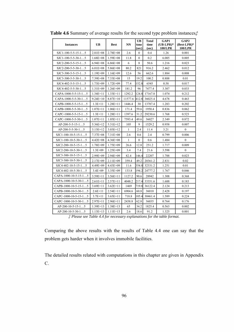
96

Table 4.6 Summary of average results for the second type problem instances‡

Instances UB Best NN

UB

tıme

(sec)

Total

time

(sec)

GAP1

(UB-LPR)*

100/LPR

GAP2

(Best-LPR)*

100/LPR

SJC1-100-5-5-15-1…5 2.81E+08 2.78E+08 2.6 0 0.4 1.26 0.001 SJC1-100-5-5-30-1…5 1.68E+08 1.59E+08 11.8 0 0.2 6.085 0.005 SJC2-200-5-5-15-1…5 6.94E+08 6.86E+08 6 8 50.6 1.216 0.023 SJC2-200-5-5-30-1…5 6.01E+08 5.86E+08 80.2 821 916.2 2.462 0.012 SJC3-300-5-5-15-1…5 1.19E+09 1.16E+09 12.6 56 662.6 1.884 0.008 SJC3-300-5-5-30-1…5 7.39E+08 7.33E+08 15 19.2 100.2 0.888 0.01 SJC4-402-5-5-15-1…5 1.73E+09 1.72E+09 77.4 152.8 6545 0.58 0.017 SJC4-402-5-5-30-1…5 1.31E+09 1.26E+09 181.2 96 7477.4 3.307 0.033

CAPA-1000-5-5-15-1…5 1.34E+11 1.33E+11 1292.2 124.8 17167.8 1.074 0.212 CAPA-1000-5-5-30-1…5 9.24E+10 8.87E+10 11577.6 412.8 36025.4 4.678 0.463 CAPB-1000-5-5-15-1…5 1.3E+11 1.28E+11 1446.4 30 13787.4 1.283 0.202 CAPB-1000-5-5-30-1…5 1.07E+11 1.06E+11 171.4 59.6 1950.4 0.836 0.062 CAPC-1000-5-5-15-1…5 1.3E+11 1.28E+11 1397.6 31.2 29230.6 1.768 0.523 CAPC-1000-5-5-30-1…5 1.07E+11 1.05E+11 7593.4 49.6 36027 2.349 0.872

AP-200-5-5-15-1…5 5.36E+12 5.31E+12 105 9 1529.2 0.958 0.007 AP-200-5-5-30-1…5 3.13E+12 3.03E+12 1 2.4 11.4 3.21 0

SJC1-100-10-5-15-1…5 7.37E+08 7.31E+08 2.6 0.6 2.4 0.799 0.006

SJC1-100-10-5-30-1…5 4.42E+08 4.36E+08 1 0 0.6 1.484 0 SJC2-200-10-5-15-1…5 1.78E+09 1.75E+09 26.6 12.8 251.2 1.717 0.009 SJC2-200-10-5-30-1…5 1.3E+09 1.25E+09 3.4 7.4 21.6 3.598 0 SJC3-300-10-5-15-1…5 2.99E+09 2.94E+09 82.4 146.4 22207 1.788 0.023 SJC3-300-10-5-30-1…5 2.17E+09 2.11E+09 359.4 49.2 20361.2 2.831 0.02 SJC4-402-10-5-15-1…5 4.49E+09 4.43E+09 11.6 354.8 32331.2 1.251 0.01 SJC4-402-10-5-30-1…5 3.4E+09 3.35E+09 133.8 194.2 24777.2 1.767 0.046

CAPA-1000-10-5-15-1…5 3.59E+11 3.56E+11 1127.2 90.6 28942 1.308 0.368 CAPA-1000-10-5-30-1…5 2.61E+11 2.57E+11 4048.2 217.4 33351.6 1.688 0.183 CAPB-1000-10-5-15-1…5 3.69E+11 3.62E+11 1469 719.8 36122.4 2.124 0.213 CAPB-1000-10-5-30-1…5 2.6E+11 2.54E+11 6904.6 60.8 36010 2.428 0.197 CAPC-1000-10-5-15-1…5 3.7E+11 3.65E+11 718.8 105.4 30461.4 1.589 0.224 CAPC-1000-10-5-30-1…5 2.97E+11 2.96E+11 2438.8 62.8 36035 0.764 0.176

AP-200-10-5-15-1…5 1.39E+13 1.38E+13 65 34.2 1825.4 0.563 0.002 AP-200-10-5-30-1…5 1.13E+13 1.11E+13 2.6 18.6 91.2 1.325 0.001

‡ Please see Table 4.4 for necessary explanations for the table format.

Comparing the above results with the results of Table 4.4 one can say that the

problem gets harder when it involves immobile facilities.

The detailed results related with computations in this chapter are given in Appendix

C.

97

CHAPTER 5

THE DYNAMIC P-MEDIAN PROBLEM

In this chapter the dynamic p-median problem is studied. A mixed integer

mathematical programming (MIP) formulation is presented and an iterative solution

algorithm which combines column generation and solving MIP models is proposed

for the problem. The heuristics and DBnP presented in the previous chapter are also

applicable for solving the dynamic p-median problem in addition to the iterative

algorithm. We solve several test problem instances in order to evaluate the

performances of our proposed solution procedures. The computational results are

discussed.

5.1 Introduction

In this chapter dynamic version of the p-median problem is studied. The p median

problem is to find the locations of p uncapacitated facilities on a graph where nodes

represent the demand sites and candidate facility location sites such that the total

allocation cost of demand nodes to open facilities is minimized. Demand amounts

change over a planning horizon as a result of many dynamic factors in time. For a

predictable planning horizon these changes can be responded by opening new

facilities or abolishing some of the existing ones. So, the dynamic p-median

problem is to determine the locations of predetermined numbers of facilities in each

period such that the total allocation cost over the planning horizon is minimized and

only opening new facilities or abolishing existing ones is allowed in a period. Note

that if the number of the facilities at a period is same with the one at the successive

period then these two periods can be aggregated and represented as a unique period.

If the numbers of the facilities at all periods are equal to each other then the

98

problem reduces to the classical p-median problem. In Chapter 4, the classical

p-median problem is explained in detail, its related literature is reviewed, and basic

modeling approaches are presented. Also, the dynamic p-median problem with

mobile facilities is studied in Chapter 4. Recall that a mathematical model, three

heuristics and a BnP algorithm are developed to solve the problem. That problem

includes the dynamic p-median problem defined above as a special case. All these

available methods can also be used for solving the dynamic p-median problem. In

this chapter the dynamic p-median problem is studied in detail. An iterative

solution algorithm, called iterative MIP based column generation algorithm

(IMCA), which is not applicable to the dynamic p-median problem with mobile

facilities, is developed for the dynamic p-median problem. The methods presented

in Chapter 4 and IMCA are used to solve the randomly generated test problem

instances. The experimental results are given.

To our best knowledge, there are two studies considering dynamic p-median

problem in the literature, one of which is a continuous location problem. Galvao

and Santibanez-Gonzalez (1992) study the problem in which the number of

facilities to be open changes according to a predetermined setting over the planning

horizon. They consider non-decreasing array of the number of the facilities and

propose a Lagrangian heuristic to minimize the sum of allocation and facility

installation costs. Drezner (1995) considers p facilities to be located one by one on

a plane over a p-period planning horizon, called “the progressive p-median

problem”. A heuristic method is presented to minimize the allocation costs. The

details of these studies are given in section 4.2.2. In the current study, no limitation

is applied on the number of the facilities, therefore it is a generalization of these

two problems.

In the following section a mathematical formulation of the dynamic p-median

problem is given. Then IMCA is presented. In the last section, computational

results are given and discussed.

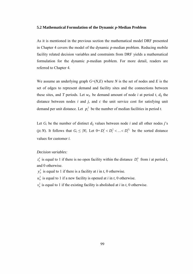
99

5.2 Mathematical Formulation of the Dynamic p-Median Problem

As it is mentioned in the previous section the mathematical model DRF presented

in Chapter 4 covers the model of the dynamic p-median problem. Reducing mobile

facility related decision variables and constraints from DRF yields a mathematical

formulation for the dynamic p-median problem. For more detail, readers are

referred to Chapter 4.

We assume an underlying graph G=(N,E) where N is the set of nodes and E is the

set of edges to represent demand and facility sites and the connections between

these sites, and T periods. Let wit be demand amount of node i at period t, dij the

distance between nodes i and j, and c the unit service cost for satisfying unit

demand per unit distance. Let 2tp be the number of median facilities in period t.

Let Gi be the number of distinct dij values between node i and all other nodes j’s

(jN). It follows that Gi ≤ |N|. Let 0= iG

iii DDD ...21 be the sorted distance

values for customer i.

Decision variables: k

itz is equal to 1 if there is no open facility within the distance k

iD from i at period t, and 0 otherwise.

2ity is equal to 1 if there is a facility at i in t, 0 otherwise. 2itu is equal to 1 if a new facility is opened at i in t, 0 otherwise. 2itv is equal to 1 if the existing facility is abolished at i in t, 0 otherwise.

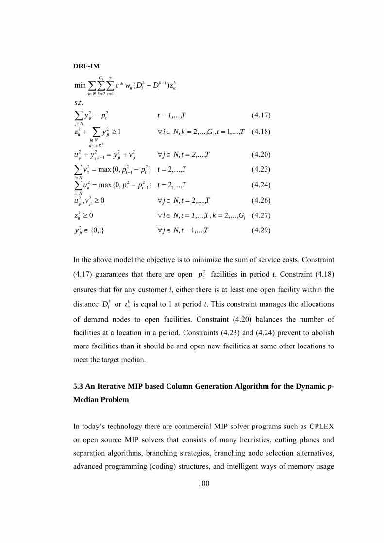
100

DRF-IM

)29.4(1}1,0{

)27.4(,...,2,0

)26.4(20,

)24.4(,...,2},0max{

)23.4(,...,2},0max{

)20.4(

)18.4(,...,1,21

)17.4(..

)(*min

2

22

21

22

221

2

2221,

2

2

22

2 1

1

T,...,t N,jy

GkT1,...,t N,iz

T,...,t N,jvu

Ttppu

Ttppv

T2,...,t N,jvyyu

TtG,...,k N,iyz

T1,...,tpy

ts

zDDwc

jt

i

k

it

jtjt

tt

Ni

it

tt

Ni

it

jtjttjjt

i

Dd

Nj

jt

k

it

t

Nj

jt

Ni

G

k

T

t

k

it

k

i

k

iit

kiji

i

In the above model the objective is to minimize the sum of service costs. Constraint

(4.17) guarantees that there are open 2tp facilities in period t. Constraint (4.18)

ensures that for any customer i, either there is at least one open facility within the

distance k

iD or k

itz is equal to 1 at period t. This constraint manages the allocations

of demand nodes to open facilities. Constraint (4.20) balances the number of

facilities at a location in a period. Constraints (4.23) and (4.24) prevent to abolish

more facilities than it should be and open new facilities at some other locations to

meet the target median.

5.3 An Iterative MIP based Column Generation Algorithm for the Dynamic p-

Median Problem

In today’s technology there are commercial MIP solver programs such as CPLEX

or open source MIP solvers that consists of many heuristics, cutting planes and

separation algorithms, branching strategies, branching node selection alternatives,

advanced programming (coding) structures, and intelligent ways of memory usage

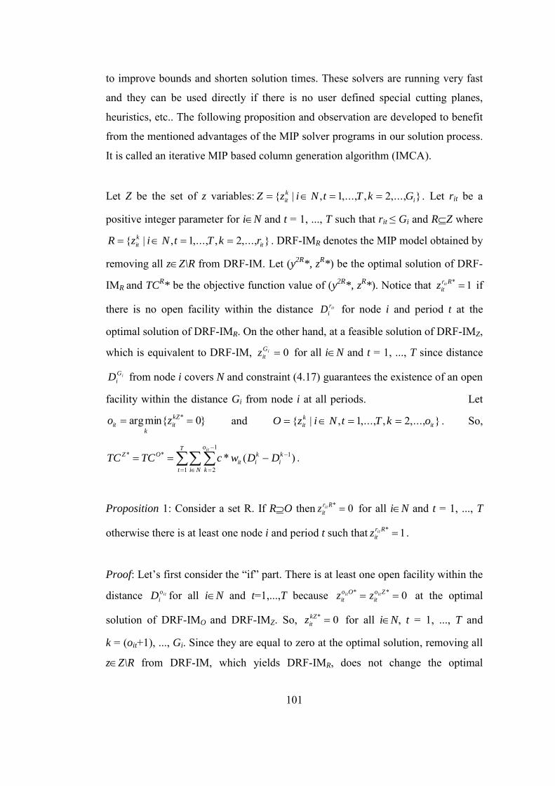
101

to improve bounds and shorten solution times. These solvers are running very fast

and they can be used directly if there is no user defined special cutting planes,

heuristics, etc.. The following proposition and observation are developed to benefit

from the mentioned advantages of the MIP solver programs in our solution process.

It is called an iterative MIP based column generation algorithm (IMCA).

Let Z be the set of z variables: },...,2,,...,1,|{ i

k

it GkTtNizZ . Let rit be a

positive integer parameter for iN and t = 1, ..., T such that rit ≤ Gi and RZ where

},...,2,,...,1,|{ it

k

it rkTtNizR . DRF-IMR denotes the MIP model obtained by

removing all zZ\R from DRF-IM. Let (y2R*, z

R*) be the optimal solution of DRF-

IMR and TCR* be the objective function value of (y2R

*, zR*). Notice that 1*

Rr

ititz if

there is no open facility within the distance itr

iD for node i and period t at the

optimal solution of DRF-IMR. On the other hand, at a feasible solution of DRF-IMZ,

which is equivalent to DRF-IM, 0iG

itz for all iN and t = 1, ..., T since distance

iG

iD from node i covers N and constraint (4.17) guarantees the existence of an open

facility within the distance Gi from node i at all periods. Let

}0{minarg * kZ

itk

it zo and },...,2,,...,1,|{ it

k

it okTtNizO . So,

T

t Ni

o

k

k

i

k

iit

OZit

DDwcTCTC1

1

2

1** )(* .

Proposition 1: Consider a set R. If RO then 0*

Rr

ititz for all iN and t = 1, ..., T

otherwise there is at least one node i and period t such that 1*

Rr

ititz .

Proof: Let’s first consider the “if” part. There is at least one open facility within the

distance ito

iD for all iN and t=1,...,T because 0**

Zo

it

Oo

ititit zz at the optimal

solution of DRF-IMO and DRF-IMZ. So, 0* kZ

itz for all iN, t = 1, ..., T and

k = (oit+1), ..., Gi. Since they are equal to zero at the optimal solution, removing all

zZ\R from DRF-IM, which yields DRF-IMR, does not change the optimal

102

solution. Because 0*

Oo

ititz and rit ≥ oit, 0*

Rr

ititz for all iN and t = 1, ..., T, and it

completes the proof of “if” part.

Now, let’s consider the “otherwise” part. Let’s consider two feasible solutions of

DRF-IMR: (y2R, z

R) and (y2R, z

R) such that y2R = y

2Z* and itr

itzR = 0 for all iN

and t = 1, ..., T. Then,

TCR=

T

tor

Ni

r

k

k

i

k

iit

T

tor

Ni

o

k

k

i

k

iit

itit

it

itit

it

DDwcDDwc1 2

1

1

1

2

1 )(*)(* ≤TCO*=TC

Z*.

Let’s consider a feasible solution for DRF-IM: (y2Z, z

Z) such that y2Z= y

2R for

all iN and t = 1, ..., T; k

itzZ= k

itzR for all iN, t = 1, ..., T and k = 2, ..., rit; and

k

itzZ = 0 for all iN, t = 1, ..., T and k = (rit +1), ..., Gi. Then, TC

R= TC

Z. There is

at least one iN and t, 1 ≤ t ≤ T such that rit < oit, (y2R, z

R) ≠ (y2Z*, z

Z*) and

TCR > TC

Z* = TC

O* ≥ TC

R. So, any solution of DRF-IMR in which all last z

variables are equal to zero cannot be optimal.□

Observation 1: According to Proposition 1, for a given set R, if 0*

Rr

ititz for all iN

and t = 1, ..., T, then y2Z* = y

2R* for all iN and t = 1, ..., T; k

itzZ*= k

itzR* for all iN,

t = 1, ..., T and k = 2, ..., rit; k

itzZ* = 0 for all iN, t = 1, ..., T and k = (rit +1), ..., Gi;

and TCZ* = TC

R*.

Observation 1 yields the following solution algorithm for DRF-IM.

Iterative MIP Based Column Generation Algorithm (IMCA)

Step 1: Choose a positive integer rit, rit ≤ Gi, for all iN and t = 1, ..., T.

Step 2: Let },...,2,,...,1,|{ it

k

it rkTtNizR and DRF-IMR be the MIP model

obtained by removing all zZ\R from DRF-IM. Solve DRF-IMR. Let (y2R*, z

R*) be

103

the optimal solution of DRF-IMR and TCR* be the objective function value of

(y2R*, z

R*).

Step 3: For all 1*

Rr

ititz , increase rits by 1 and go to Step 2.

Step 4: STOP. The optimal solution of DRF-IM, (y2Z*, z

Z*), and its objective

function value TCZ* is: y2Z

* = y2R

* for all iN and t = 1, ..., T; k

itzZ* = k

itzR* for all

iN, t = 1, ..., T, and k = 2, ..., rit; k

itzZ* = 0 for all iN, t = 1, ..., T, and

k = (rit +1), ..., Gi; and TCZ* = TC

R*.

Note that in each iteration of IMCA a MIP model (DRF-IMR) is solved first and

then column generation is applied by using the integer optimal solution. The MIP

model is adjusted using the generated columns for the next iteration.

Choosing very small r values in step 1 of IMCA may cause too many iterations and

long solution times. Since in each iteration of IMCA a MIP model is solved, such

an act may cause significant increases in solution times. In order to shorten the

solution times and benefit from the advantages of the commercial MIP solvers,

initial r values will be very important on the performance of IMCA. As mentioned

in Chapter 4 for the location problems with uncapacitated facilities, generally linear

relaxations of the MIP models consisting of Balinski type constraints give good

lower bounds and the relaxed solutions are close to the integer optimal solutions.

Solution of the LP relaxation of the Model 5 and Model 6 in section 4.2.1 is same

as the solution of the LP relaxation of Model 1 in that section. (Elloumi 2010;

Garcia et al. 2011) When T=1, the resultant dynamic p-median problem is the p-

median problem and DRF-IM reduces to Model 6. Although DRF-IM does not

involve Balinski constraints, its LP relaxation gives the same solution with the

model consisting of Balinski constraints. Given that the LP relaxation of DRF-IM

generally gives good lower bounds and the solution of the LP relaxation of DRF-

IM is close to the integer optimal solution of DRF-IM. We determine initial r

values in step 1 of IMCA by using the solution of LP relaxation of DRF-IM.

104

Let zLP be the solution of LP relaxation of DRF-IM. For node i and period t the

initial rit value in step 1 of IMCA is determined by }0{minarg kLP

itk

it zr .

In order to solve the LP relaxation of DRF-IM the BnP procedure presented in

Chapter 4 is used only for the root node of the search tree.

5.4 Computational Results

We perform our computations on the test problem instances used in Chapter 4.

These test problem instances are considered in two groups: (1) benchmarking p-

median problem instances from the literature, and (2) randomly generated dynamic

p-median problem instances. The instances in the second group are partitioned into

two disjoint subsets, A and B. The first group consists of 27 instances with 900

nodes. The set A of the second group consists of 60 instances with 100, 200, and

300 nodes and 5 and 10 periods. The set B of the second group consists of 100

instances with 200, 402, and 1,000 nodes and 5 and 10 periods (for details see

section 4.5).

We use two platforms during our computations: (1) a 3.10 GHz PC with 6 GB

RAM, (2) a 2.66 GHz PC with 1.93 GB RAM. In all computations CPLEX 12.3 is

used as an LP and MIP solver. Our heuristics and DBnP algorithm are coded with

C++ programming language.

The solution times, the relative deviations from the lower bounds and the numbers

of optimally solved instances in a limited time are used as our criteria to evaluate

the performances of proposed methods.

Our computational study consists of two parts for the methods presented in Chapter

4: (1) deciding on parameter setting for the algorithm on a subset of our dynamic

test problem instances, and (2) assessments of performances of our algorithms on a

larger set of dynamic test problem instances. Similarly, our computational study

105

consists of two parts for IMCA: (1) validation, and (2) assessment of performance

of IMCA on a set of dynamic test problem instances.

Below, first we perform our computations by the previously presented heuristics

and DBnP, and then we apply IMCA.

5.4.1 Performances of the Heuristics and DBnP in Chapter 4

Computations are performed on our first computer.

A. Testing Performances of Heuristics and Parameter Setting

We use test instances in the set A of second group to evaluate performances of

heuristics and to determine the target value for DBnP procedure. We choose period

1, period 3, and period 5 as the starting period h for myopic heuristic MH for the

instances with five periods. We choose period 1, period 4, period 7, and period 10

as the starting period h for the instances with ten periods. For our progressive

heuristics P1 and P2, we start with the first and last periods of the reordered and

combined periods of the original problem instances.

Average solution times and average relative gaps between the upper bounds (UB)

obtained by the heuristics and the lower bounds obtained by the linear relaxations

(LPR) of the models are given in Table 5.1. Note that each row of Table 5.1

displays average values of 30 test problem instances.

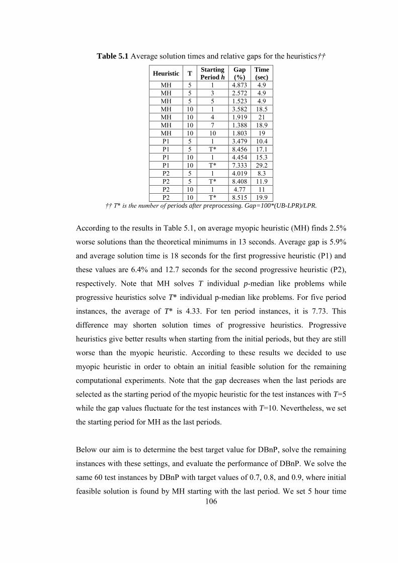
106

Table 5.1 Average solution times and relative gaps for the heuristics††

Heuristic T Starting

Period h

Gap

(%)

Time

(sec)

MH 5 1 4.873 4.9 MH 5 3 2.572 4.9 MH 5 5 1.523 4.9 MH 10 1 3.582 18.5 MH 10 4 1.919 21 MH 10 7 1.388 18.9 MH 10 10 1.803 19 P1 5 1 3.479 10.4 P1 5 T* 8.456 17.1 P1 10 1 4.454 15.3 P1 10 T* 7.333 29.2 P2 5 1 4.019 8.3 P2 5 T* 8.408 11.9 P2 10 1 4.77 11 P2 10 T* 8.515 19.9

†† T* is the number of periods after preprocessing. Gap=100*(UB-LPR)/LPR.

According to the results in Table 5.1, on average myopic heuristic (MH) finds 2.5%

worse solutions than the theoretical minimums in 13 seconds. Average gap is 5.9%

and average solution time is 18 seconds for the first progressive heuristic (P1) and

these values are 6.4% and 12.7 seconds for the second progressive heuristic (P2),

respectively. Note that MH solves T individual p-median like problems while

progressive heuristics solve T* individual p-median like problems. For five period

instances, the average of T* is 4.33. For ten period instances, it is 7.73. This

difference may shorten solution times of progressive heuristics. Progressive

heuristics give better results when starting from the initial periods, but they are still

worse than the myopic heuristic. According to these results we decided to use

myopic heuristic in order to obtain an initial feasible solution for the remaining

computational experiments. Note that the gap decreases when the last periods are

selected as the starting period of the myopic heuristic for the test instances with T=5

while the gap values fluctuate for the test instances with T=10. Nevertheless, we set

the starting period for MH as the last periods.

Below our aim is to determine the best target value for DBnP, solve the remaining

instances with these settings, and evaluate the performance of DBnP. We solve the

same 60 test instances by DBnP with target values of 0.7, 0.8, and 0.9, where initial

feasible solution is found by MH starting with the last period. We set 5 hour time

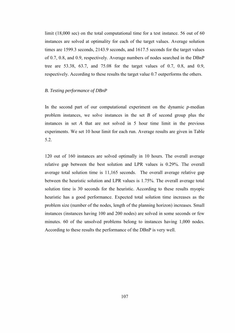
107

limit (18,000 sec) on the total computational time for a test instance. 56 out of 60

instances are solved at optimality for each of the target values. Average solution

times are 1599.3 seconds, 2143.9 seconds, and 1617.5 seconds for the target values

of 0.7, 0.8, and 0.9, respectively. Average numbers of nodes searched in the DBnP

tree are 53.38, 63.7, and 75.08 for the target values of 0.7, 0.8, and 0.9,

respectively. According to these results the target value 0.7 outperforms the others.

B. Testing performance of DBnP

In the second part of our computational experiment on the dynamic p-median

problem instances, we solve instances in the set B of second group plus the

instances in set A that are not solved in 5 hour time limit in the previous

experiments. We set 10 hour limit for each run. Average results are given in Table

5.2.

120 out of 160 instances are solved optimally in 10 hours. The overall average

relative gap between the best solution and LPR values is 0.29%. The overall

average total solution time is 11,165 seconds. The overall average relative gap

between the heuristic solution and LPR values is 1.75%. The overall average total

solution time is 30 seconds for the heuristic. According to these results myopic

heuristic has a good performance. Expected total solution time increases as the

problem size (number of the nodes, length of the planning horizon) increases. Small

instances (instances having 100 and 200 nodes) are solved in some seconds or few

minutes. 60 of the unsolved problems belong to instances having 1,000 nodes.

According to these results the performance of the DBnP is very well.

108

Table 5.2 Summary of average results for the instances in the second group and

DBnP‡

Instances UB Best NN

UB

tıme

(sec)

Total

time

(sec)

GAP1

(UB-LPR)*

100/LPR

GAP2

(Best-LPR)*

100/LPR

SJC1-100-5-5-15-1…5 2.85E+08 2.81E+08 1.8 0.01 0.2 1.311 0.002 SJC1-100-5-5-30-1…5 1.62E+08 1.62E+08 1 0.01 0.02 0.589 0 SJC2-200-5-5-15-1…5 7.06E+08 6.99E+08 190.6 3.6 263.8 1.043 0.06 SJC2-200-5-5-30-1…5 5.99E+08 5.92E+08 7.4 2.6 6 1.252 0.004 SJC3-300-5-5-15-1…5 1.2E+09 1.18E+09 5 16.6 177.6 1.587 0.003 SJC3-300-5-5-30-1…5 7.63E+08 7.46E+08 123 6.6 400.6 2.368 0.036 SJC4-402-5-5-15-1…5 1.77E+09 1.75E+09 18 112.2 3594 1.359 0.045 SJC4-402-5-5-30-1…5 1.3E+09 1.28E+09 12.4 79.6 1078.8 1.609 0.016

CAPA-1000-5-5-15-1…5 1.37E+11 1.36E+11 1503.2 30.6 16614.6 1.566 0.84 CAPA-1000-5-5-30-1…5 9.09E+10 8.94E+10 1462.6 14.8 6389.6 2.021 0.38 CAPB-1000-5-5-15-1…5 1.31E+11 1.3E+11 292.6 19 3410.4 1.175 0.31 CAPB-1000-5-5-30-1…5 1.09E+11 1.08E+11 1960.4 20.4 12045.6 1.204 0.388 CAPC-1000-5-5-15-1…5 1.32E+11 1.31E+11 1457.2 19.6 22519.8 2.042 1.176 CAPC-1000-5-5-30-1…5 1.08E+11 1.06E+11 7005.8 25.4 36014.6 2.588 0.571

AP-200-5-5-15-1…5 5.51E+12 5.41E+12 2.6 6.2 37.4 1.993 0.042 AP-200-5-5-30-1…5 3.16E+12 3.1E+12 1 1.8 4 1.804 0

SJC1-100-10-5-15-1…5 7.55E+08 7.42E+08 80.4 0.4 14.6 1.818 0.048

SJC1-100-10-5-30-1…5 4.49E+08 4.43E+08 1.4 0 0.2 1.487 0.001 SJC2-200-10-5-15-1…5 1.8E+09 1.77E+09 15 6.6 177.8 1.535 0.007 SJC2-200-10-5-30-1…5 1.29E+09 1.27E+09 3.4 4.8 12.6 1.749 0.002 SJC3-300-10-5-15-1…5 3.02E+09 2.98E+09 197 65.8 22926.2 1.71 0.244 SJC3-300-10-5-30-1…5 2.17E+09 2.13E+09 398.2 37.4 9439.2 1.876 0.074 SJC4-402-10-5-15-1…5 4.56E+09 4.49E+09 18.4 139.8 29687 1.585 0.075 SJC4-402-10-5-30-1…5 3.43E+09 3.39E+09 186.8 77.2 20007.8 1.396 0.081

CAPA-1000-10-5-15-1…5 3.67E+11 3.62E+11 484.4 47.4 27571.8 2.398 1.003 CAPA-1000-10-5-30-1…5 2.64E+11 2.61E+11 2149.6 21.4 28885.4 1.764 0.568 CAPB-1000-10-5-15-1…5 3.72E+11 3.67E+11 356.8 48.6 29431.6 2.09 0.586 CAPB-1000-10-5-30-1…5 2.62E+11 2.57E+11 873.8 23.4 21952.8 2.052 0.193 CAPC-1000-10-5-15-1…5 3.77E+11 3.72E+11 283.8 65 28987.6 2.201 0.962 CAPC-1000-10-5-30-1…5 3.07E+11 3.02E+11 1893.8 41.2 35386 2.557 0.813

AP-200-10-5-15-1…5 1.43E+13 1.4E+13 2.2 11.6 197.8 2.483 0.001 AP-200-10-5-30-1…5 1.13E+13 1.12E+13 4.2 9.4 71.4 1.038 0.002

‡ Test problem instances are given in the first column. Test problem instances are labeled as

NAME-Number of the nodes (|N|)-Length of the planning horizon (T)-Lower bound parameter of the

discrete uniform distribution that the numbers of medians are generated from-Upper bound

parameter of the discrete uniform distribution that the numbers of medians are generated from-

Instance number. Instance number 1...5 shows that average values are given in the corresponding

row and obtained from the solutions of instances 1, ..., 5. In the second column upper bound values

obtained by the myopic heuristic are given. In the third column best solution values are given, found

by DBnP in 36,000 seconds. In the fourth column the numbers of nodes of the BnB tree explored are

given. In the next two columns, solution time for myopic heuristic and the total solution time

(including the solution time of the heuristic) are given, respectively.

109

5.4.2 Performance of IMCA

A. Validation of IMCA

Before dealing with the dynamic problems, we first solve the test problem instances

in the first group in order to validate IMCA. Although these computations are

mainly for validation purpose, solution times show that our algorithm competes

with Avella et al. (2007) and Garcia et al. (2011), which are two recent and

outstanding studies in the literature. Solution times are given in Table 5.3.

Computations are performed on our first computer platform.

Roughly speaking, our computer is 1.7 times faster than Avella et al. (2007) and 1.3

times faster than Garcia et al. (2011). According to the overall results, we solve all

instances faster than Avella et al. (2007) and 21 of the 27 instances faster than

Garcia et al. (2011) by IMCA. IMCA dominates the DBnP. Average solution times

are 40 seconds for Avella et al. (2007), 6.13 seconds for Garcia et al. (2007), 19.2

seconds for DBnP, and 4.6 seconds for IMCA. So, on average IMCA is the best.

Although these computations are mainly for validation purpose of IMCA, the

solution times show that it competes with outstanding studies in the literature.

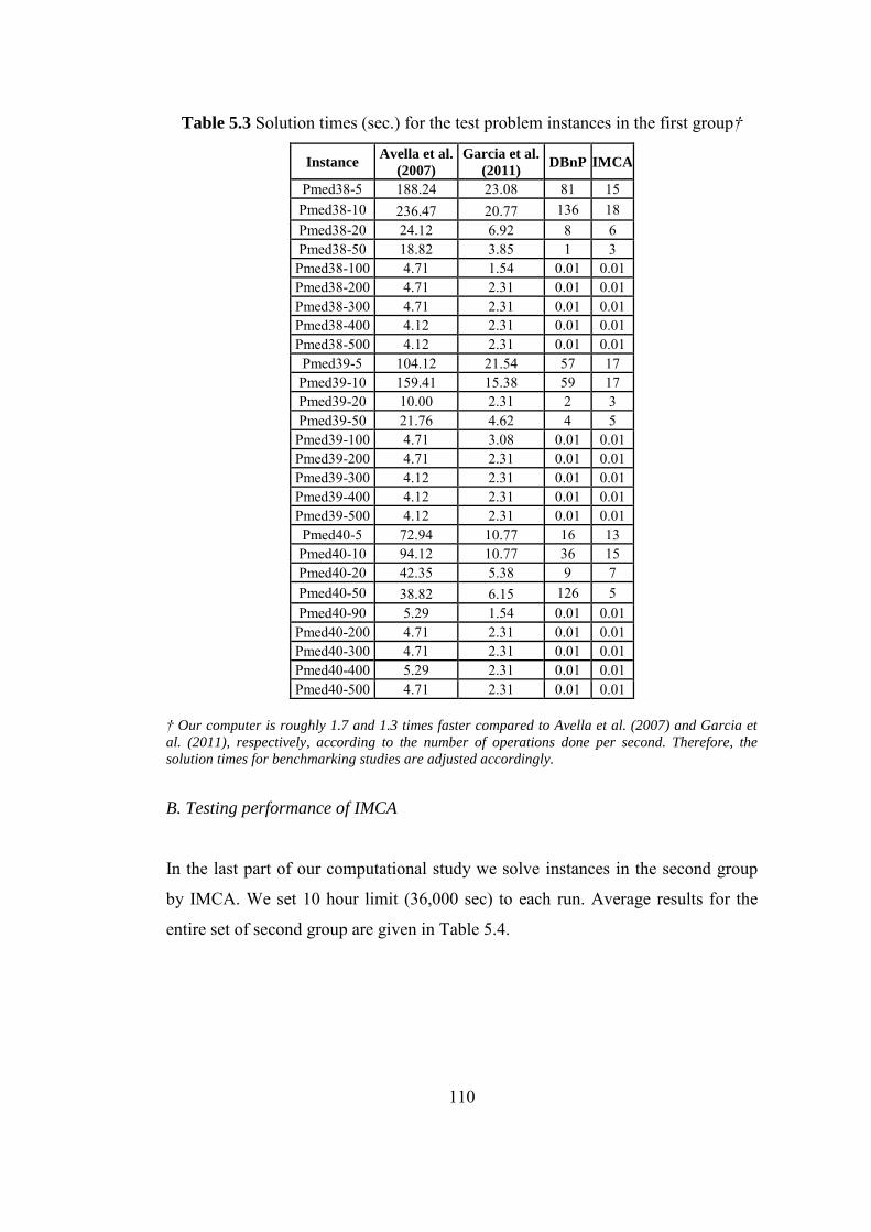
110

Table 5.3 Solution times (sec.) for the test problem instances in the first group†

Instance Avella et al.

(2007)

Garcia et al.

(2011) DBnP IMCA

Pmed38-5 188.24 23.08 81 15 Pmed38-10 236.47 20.77 136 18 Pmed38-20 24.12 6.92 8 6 Pmed38-50 18.82 3.85 1 3

Pmed38-100 4.71 1.54 0.01 0.01 Pmed38-200 4.71 2.31 0.01 0.01 Pmed38-300 4.71 2.31 0.01 0.01 Pmed38-400 4.12 2.31 0.01 0.01 Pmed38-500 4.12 2.31 0.01 0.01 Pmed39-5 104.12 21.54 57 17 Pmed39-10 159.41 15.38 59 17 Pmed39-20 10.00 2.31 2 3 Pmed39-50 21.76 4.62 4 5

Pmed39-100 4.71 3.08 0.01 0.01 Pmed39-200 4.71 2.31 0.01 0.01 Pmed39-300 4.12 2.31 0.01 0.01 Pmed39-400 4.12 2.31 0.01 0.01 Pmed39-500 4.12 2.31 0.01 0.01 Pmed40-5 72.94 10.77 16 13 Pmed40-10 94.12 10.77 36 15 Pmed40-20 42.35 5.38 9 7 Pmed40-50 38.82 6.15 126 5 Pmed40-90 5.29 1.54 0.01 0.01

Pmed40-200 4.71 2.31 0.01 0.01 Pmed40-300 4.71 2.31 0.01 0.01 Pmed40-400 5.29 2.31 0.01 0.01 Pmed40-500 4.71 2.31 0.01 0.01

† Our computer is roughly 1.7 and 1.3 times faster compared to Avella et al. (2007) and Garcia et

al. (2011), respectively, according to the number of operations done per second. Therefore, the

solution times for benchmarking studies are adjusted accordingly.

B. Testing performance of IMCA

In the last part of our computational study we solve instances in the second group

by IMCA. We set 10 hour limit (36,000 sec) to each run. Average results for the

entire set of second group are given in Table 5.4.

111

Table 5.4 Summary of average results for the dynamic p-median problem instances

and IMCA‡

Instances UB Best NN

UB

tıme

(sec)

Total

time

(sec)

GAP1

(UB-LPR)*

100/LPR

GAP2

(Best-LPR)*

100/LPR

SJC1-100-5-5-15-1…5 2.84E+08 2.81E+08 1 0.6 1.4 1.154 0.002 SJC1-100-5-5-30-1…5 1.64E+08 1.62E+08 1 0 0.4 1.234 0 SJC2-200-5-5-15-1…5 7.08E+08 6.99E+08 3.4 7 55.4 1.312 0.061 SJC2-200-5-5-30-1…5 5.99E+08 5.92E+08 1 5 15.2 1.226 0.004 SJC3-300-5-5-15-1…5 1.19E+09 1.18E+09 1 32.8 296.4 1.191 0.003 SJC3-300-5-5-30-1…5 7.64E+08 7.46E+08 22 15.2 149.6 2.517 0.036 SJC4-402-5-5-15-1…5 1.77E+09 1.75E+09 14.8 105.6 2027.8 1.365 0.045 SJC4-402-5-5-30-1…5 1.3E+09 1.28E+09 5 73.4 259.4 1.21 0.017

CAPA-1000-5-5-15-1…5 1.37E+11 1.33E+11 731.2 32.2 3764 2.795 0.144 CAPA-1000-5-5-30-1…5 9.09E+10 8.84E+10 120.8 15.2 419.4 2.843 0.203 CAPB-1000-5-5-15-1…5 1.32E+11 1.28E+11 70.8 21.2 861.4 2.594 0.080 CAPB-1000-5-5-30-1…5 1.09E+11 1.06E+11 175.8 20 819.2 2.937 0.070 CAPC-1000-5-5-15-1…5 1.32E+11 1.28E+11 2611 20.4 11048.8 3.026 0.813 CAPC-1000-5-5-30-1…5 1.08E+11 1.04E+11 550.8 27.4 1458.8 3.395 0.153

AP-200-5-5-15-1…5 5.53E+12 5.41E+12 4 6 38.4 2.248 0.042 AP-200-5-5-30-1…5 3.15E+12 3.1E+12 1 1.8 3.4 1.344 0

SJC1-100-10-5-15-1…5 7.56E+08 7.42E+08 4.6 1.4 5.6 1.93 0.048

SJC1-100-10-5-30-1…5 4.5E+08 4.43E+08 1 0.6 1.8 1.615 0.001 SJC2-200-10-5-15-1…5 1.81E+09 1.79E+09 33.2 14 220.8 1.625 0.06 SJC2-200-10-5-30-1…5 1.29E+09 1.27E+09 1 7.4 27.2 1.71 0.002 SJC3-300-10-5-15-1…5 3.02E+09 2.98E+09 722.2 67 11466.4 1.642 0.144 SJC3-300-10-5-30-1…5 2.16E+09 2.13E+09 153 38.8 2302.4 1.42 0.061 SJC4-402-10-5-15-1…5 4.54E+09 4.49E+09 55.6 180.2 16254.2 1.163 0.047 SJC4-402-10-5-30-1…5 3.42E+09 3.38E+09 118.4 104.4 6861.4 1.079 0.055

CAPA-1000-10-5-15-1…5 3.66E+11 3.62E+11 1911.2 40.4 23958.8 3.138 2.127 CAPA-1000-10-5-30-1…5 2.65E+11 2.59E+11 977.2 23.4 9827 2.789 0.841 CAPB-1000-10-5-15-1…5 3.72E+11 3.64E+11 230.6 47.4 12173.4 2.984 1.012 CAPB-1000-10-5-30-1…5 2.61E+11 2.54E+11 56.8 23.6 1057.2 2.702 0.116 CAPC-1000-10-5-15-1…5 3.76E+11 3.73E+11 1031.8 50 16410.8 3.153 2.279 CAPC-1000-10-5-30-1…5 3.05E+11 3.02E+11 3984 28.8 19354.2 3.225 2.109

AP-200-10-5-15-1…5 1.42E+13 1.4E+13 1 12.2 145 1.5 0.002 AP-200-10-5-30-1…5 1.13E+13 1.12E+13 1 9.6 41.8 0.955 0.002

‡ Since the table format is same with see the explanation of Table 5.2.

148 of 160 instances are solved optimally in 10 hours. The overall average total

solution time is 4416 seconds. According to these results, the performance of

IMCA is better than the performance of DBnP. So, the main motivation for

developing IMCA, benefit from the advantages of the today’s technology and MIP

solver programs, is validated by these results.

The detailed results are given in Appendix D.

112

CHAPTER 6

CONCLUSION

In this thesis four location problems are studied. The first problem is about the

location of depots and quarries in a highway construction project. The second

problem is about the location of mobile and immobile concrete batching facilities

for a railroad construction project. Both problems are motivated by real life

applications. The third problem generalizes our findings for the second problem to

general networks under the p-median problem settings. The resultant problem is a

dynamic version of the p-median problem with mobile facilities. The fourth

problem is a special case of the third problem where all facilities are assumed to be

immobile.

The first problem is a new location problem, called the depot-quarry location

problem, and occurs in road construction projects. Two mixed integer programming

formulations for the problem are developed. The first formulation is the fixed

charge network flow problem formulation. Using the optimal solution properties of

the fixed charge network flow problem, the shortest path problem formulation of

the problems is developed. A dynamic programming algorithm is presented for the

depot-quarry location problem.

The depot-quarry location problem is tightly related with the uncapacitated lot

sizing problem with backlogging. Although its dynamic programming algorithm

runs in polynomial time, its running complexity is higher than that of dynamic

programming algorithm of the uncapacitated lot sizing problem with backlogging.

It is shown that the depot-quarry location problem is a generalization of the

uncapacitated lot sizing problem with backlogging.

113

The second problem is also a new problem, called the dynamic, capacitated location

problem with mobile and immobile facilities. It occurs in railroad construction

projects. A mixed integer linear programming model is developed to solve the

problem. It is also shown how the model can be used to solve similar problems in

the literature with simple modifications.

We provide computational results for a case study problem based on a real project

data. A sensitivity analysis is carried on the solution of the case problem. It is seen

that a larger percent of the total cost is due to transportation costs and the solution

remains almost unchanged even after facility costs are substantially changed.

Observing the demand planned in the project schedule is sparse in location and time

basis, it is concluded that more reductions in the total cost would be achieved if

location-allocation and project scheduling decisions had been made simultaneously.

If construction schedules in the projects are prepared in weekly bases, which is

preferable in terms of better planning and managing work and workforce, the

number of periods can increase up to hundreds even for a small scale project. In

order to solve such larger sized problems in reasonable times, a fast preprocessing

heuristic is proposed to reduce the number of candidate location sites. The

performance of the heuristic is tested on a set of test problem instances, including

the case problem. The heuristic reduces running times of the model substantially

with a slight change on the solution quality.

The dynamic demands and mobile facilities are two distinctive properties of the

second problem. Being motivated by these rich properties, the second problem is

generalized to the general networks under the p-median problem settings, called the

dynamic p-median problem with mobile facilities. To the best of our knowledge,

this is the first study in the location literature that combines important decision

components of the known dynamic p-median problems into a single decision

framework. Two classes of the problem are considered. In the first problem class,

all facilities are assumed to be mobile while facilities are assumed to be mobile,

immobile, or both types in the second class. Three constructive heuristics and a

114

branch and price algorithm are proposed to solve the problem. Performances of

these solution procedures are tested on randomly generated instances with up to

1000 nodes and 10 periods. It is shown that the heuristics’ performances change

according to the problem classes and the first heuristic, called the myopic heuristic,

outperforms other two progressive heuristics with 0.2% and 1.8% deviations from

the lower bound in 54 seconds and 2 minutes computation times on average for the

first and second classes, respectively.

The proposed branch and price algorithm is validated over the well-known p-

median problem instances from the literature. Besides the validation, it is shown

that the algorithm competes with the best p-median algorithms in the literature. The

algorithm’s performance is assessed on the dynamic problem test instances, which

are generated systematically and introduced for the first time as the benchmark test

instances into the computational literature. Our empirical results show that the

algorithm performs well. Most large instances are solved at optimality within a

given time limit of 10 hours. The average solution times are approximately 1 hour

for the first problem class and 4 hours for the second problem class.

According to our numerical results for the performance of the first heuristic and the

branch and price algorithm, it may be concluded that the second problem class is

harder than the first problem class. This result can easily be justified because one

should consider later periods of the planning horizon when deciding on the

locations of immobile facilities for the second class. The mobile facilities are

flexible for responding the changes in demand over time.

In the fourth problem, we consider a special case of the third problem, allowing

only conventional (immobile) facilities. Although the heuristics and the branch and

price algorithm presented for the third problem are also applicable to the current

problem, the branch and price algorithm is modified to take advantage of single

type immobile facility. That iterative algorithm combines column generation and

mixed integer programming solutions in an iterative way. The algorithms’

performances are evaluated by the computational experiments on the randomly

115

generated problem instances and results are presented. 120 of 160 instances are

solved optimally by the branch and price method. The average solution time is

approximately 3 hours. The iterative algorithm is validated over the p-median

problem instances from the literature. It is seen that the new algorithm is better than

the best studies in the literature. Then it is tested on the randomly generated

dynamic problem instances. 147 of 160 instances are solved optimally. The average

solution time is about 75 minutes. As a result it outperforms the branch and price

algorithm.

Even the proposed branch and price algorithm competes with the best studies in the

literature on the p-median problem instances, on average Garcia et al. (2011) is

approximately 3 times faster than the present branch and price algorithm. The

modules in the C++ code of the algorithm may be improved. Furthermore, instead

of depth first search breath first search may be used. Some other node and

branching variable selection strategies may be explored in order to improve the

performance of the branch and price algorithm.

Future Study Directions

Including some rich features to the depot-quarry location problem such as a general

cost structure, capacity levels for depots and quarries, and capacitated trucks for

transportation of materials might be an interesting future research area.

More effective solution procedures might be developed by using the line property

of the second problem. After production schedules are prepared for the art

buildings, starting periods to construct buildings and location-allocation decisions

might be considered simultaneously. Vehicle scheduling and routing decisions

might also be included to these studies.

An apparent extension of the dynamic p-median problem with mobile facilities is to

consider the dynamic fixed charge facility location problem with mobile facilities.

The proposed solution methods for the dynamic p-median problem can be adapted

116

to the fixed charge version of the problem. Instead of facility abolishing, only

facility closure and reopening cases can be considered in all of these problems.

117

REFERENCES

Adlakha, V. and Kpwalski, K., 1999. “On the fixed charge transportation problem”, Omega, Int. J. Mgmt. Sci., 27, 381-388. Antunes, A. and Peeters, D., 2000. “A dynamic optimization model for school network planning”, Socio-Economic Planning Sciences, 34, 101-120. Antunes, A. and Peeters, D., 2001. “On solving complex multi-period location models using simulated annealing”, European Journal of Operational Research, 130,190-201. Arabani, A.B. and Farahani, R.Z., 2012. “Facility location dynamics: an overview of classifications and applications”, Computers and Industrial Engineering, 62, 408-420. Avella, P. and Sassano, A., 2001. “On the p-median polytope”, Mathematical

Programming, 89, 395-411. Avella, P., Sassano, A. and Vasil’ev, I., 2007. “Computational study of large-scale p-median problems”, Mathematical Programming (Ser. A), 109, 89-114. Balinski, M., 1965. “Integer programming methods, uses and computation”, Management Science (Ser. A), 12, 253-313. Ballou, R. H., 1968. “Dynamic warehouse location analysis”, Journal of Marketing

Research, 5, 271-276. Beasley, J.E., 1985. “A note on solving large p-median problems”, European

Journal of Operational Research, 21, 270-273. Beasley, J.E., 1988. “An algorithm for solving large capacitated warehouse location problems”, European Journal of Operational Research, 33, 314-325. Beasley, J.E., 1993. “Lagrangian heuristics for location problems”, European

Journal of Operational Research, 65, 383-399. Beltran, J. L. and Krass, D., 2002. “Dynamic lot sizing with returning items and disposals”, IIE Transactions, 34, 437-448. Berberler, M.E., Çalışkan, A., Nuriyev, U.G. and Şahiner., B., 2011. “Algorithm to facility location problem on a line”, World Applied Sciences Journal, 13(12), 2436-2443.

118

Brimberg, J. and M., Mehrez, A., 2001. “Location and sizing of facilities on a line”, Top, 9(2), 271-280. Brimberg, J., Korach, E., Eben-Chaime, M., Mehrez, A., 2001. “The capacitated p-facility location problem on the real line”, International TraIMCActions in

operational Research, 8, 727-738. Brimberg, J. and ReVelle, C., 1998. “Solving the plant location problem on a line by linear prograsmming”, Top, 6 (2), 277-286. Canel, C., and Khumawala, B. M. (1997). Multi-period international facilities location: an algorithm and application. International Journal of Production

Research, 35(7), 1891-1910. Captivo, E.M., 1991. “Fast primal and dual heuristics for the p-median location problem”, European Journal of Operational Research, 52, 65-74. Chardaire P., Sutter A., and Costa M. (1996). Solving the dynamic facility location problem. Networks, 28, 117-124. Christofides, N. and Beasley, J.E., 1982. “A tree search algorithm for the p-median problem”, European Journal of Operational Research, 10, 196-204. Church, R.L., 2003. “COBRA: a new formulation of the classical p-median location problem”, Annals of Operations Research, 122, 103-120. Church, R.L., 2008. “BEAMR: an exact and approximate model for the p-median problem”, Computers and Operations Research, 35, 417-426. Contreras, I., Cordeau, J. and Laporte, G., 2011. “The dynamic uncapacitated hub location problem”, Transportation Science, 45, 18-32. Cornuejols, G., Fisher, M.L. and Nemhauser, G.L., 1977. “Location of bank accounts to optimize float: an analytic study of exact and approximate algorithms”, Management Science, 23, 789-810. Cornuejols, G., Nemhauser, G. and Wolsey, L.A., 1980. “A canonical representation of simple plant location problems and its applications”, SIMAX 1(3),261–272 Cornuejols, G., Nemhauser, G. and Wolsey, L.A., 1990. “The uncapacitated facility location problem”, In: Mirchandani PB, Francis RL (eds) Discrete location theory, Wiley, New York. Current, J., Ratick, S. and ReVelle, C., 1997. “Dynamic facility location when the total number of facilities uncertain: a decision analysis approach”, European

Journal of Operational Research, 110, 597-609.

119

de Farias (Jr.), I.R., 2001. “A family of facets for the uncapacitated p-median polytope”, Operations Research Letters, 28, 161-167. Dias, J., Captivo, M.E., and Climaco, J. (2006). Capacitated dynamic location problems with opening, closure and reopening of facilities. IMA Journal of

Management Mathematics, 17 (4), 317–348. Dias J, Captivo M. E., and Climaco J. (2007). Efficient primal-dual heuristic for a dynamic location problem. Computers and Operations Research, 34, 1800-1823. Drezner, Z., 1995. “Dynamic Location Problem: The progressive p-median problem”, Location Science, 3 (1), 1-7. Eben-Chaime, M., Mehrez, A., Markovich, G., 2002. “Capacitated location-allocation problems on a line”, Computers and Operations Research, 29, 459-470. Efroymson, M. and Ray, T., 1966. “A branch and bound algorithm for plant location”, Operations Research, 14, 361-368.

Elloumi, S., 2010. “A tighter formulation of the p-median problem”, J. Combin.

Optim., 19 (1), 69-83. Elloumi, S. and Plateau, A., 2010. “A computational study for the p-median problem”, Electronic Notes in Discrete Mathematics, 36, 455-462. El-Shaieb, A.M., 1973. “A new algorithm for locating sources among destinations”, Management Science, 20, 221-231. Epstein R., Weintraub A., Sapunar P., Nieto E., Sessions J. B., Sessions J., Bustamante F., and Musante H. (2006). A combinatorial heuristic approach for solving real-sized machinery location and road design problems in forestry planning. Operations Research, 54(6), 1017-1027. Erlenkotter, D., 1978. “A dual-based procedure for uncapacitated facility location”, Operations Research, 26, 992-1009. Erlenkotter, D., 1981. “A comparative study of approaches to dynamic location problems”, European Journal of Operational Research, 6, 133-143. Farahani, R.Z., Drezner, Z. and Asgari, N., 2009. “Single facility location and relocation problem with time dependent weights and discrete planning horizon”, Annals of Operations Research, 167, 353-368. Federgün, A. and Truz, M., 1991. “A simple forward algorithm to solve general dynami lot sizing models with n periods in O(n log n) or O(n) time”, Management

Science, 37, 1067-1087.

120

Feldman, E., Lehrer, F.A. and Ray, T.L., 1966. “Warehouse locations under continuous economies of scale”, Management Science, 12, 670-684. Francis, R.L., Lowe, T.J. and Tamir, A., 2000. “Aggregation error bounds for a class of location models”, Operations Research, 48, 294-307. Frantzeskakis, M. and Watson-Gandy, C.D.T., 1989. “The use of state space relaxation for the dynamic facility location problem”, Annals of Operations

Research, 18, 189-212. Galvao, R.D., 1980. “A dual-bounded algorithm for the p-median problem”, Operations Research, 28(5), 1112-1121. Galvao, R.D., 1993. “Use of Lagrangean relaxation in the solution of uncapacitated facility location problems”, Location Science, 1, 57-70. Galvao, R.D. and Santibanez-Gonzales, E., 1992. “A Lagrangean heuristic for the pk-median dynamic location problem”, European Journal of Operational Research, 58, 250-262. Galvao, R.D. and Raggi, L.A., 1989. “A method for solving to optimality uncapacitated location problems”, Annals of Operations Research, 18, 225-244. Garcia, S., Labbe, M. and Marin, A., 2011. “Solving large p-median problems with a radius formulation”, INFORMS Journal on Computing, 23 (4), 546-556. Garfinkel, R.S., Neebe, A.W. and Rao, M.R., 1974. “An algorithm for the m-median plant location problem”, Transportation Science, 8, 217-236. Gourdin, E., and Klopfenstein, O. (2008). Multi-period capacitated location with modular equipments. Computers and Operations Research, 35, 661-682. Hakimi, S. L., 1964. “Optimum locations of switching centers and the absolute centers and medians of a graph”, Operations Research, 12, 450-459. Hakimi, S. L., 1965. “Optimum distribution of switching centers in a communication network and some related graph theoretic problems”, Operations

Research, 13, 462-475. Hanjoul, P., and Peeters, D., 1985. “A comparison of two dual-based procedures for solving the p-median problem”, European Journal of Operational Research, 20, 387-396. Hribar, M. and Daskin, M., 1997. “A dynamic programming heuristic for the p-median problem”, European Journal of Operational Research, 101, 499-508.

121

Hsu, V. N., Lowe, T. J., Tamir, A., 1997. “Structured p-facility location problems on the line solvable in polynomial time”, Operations Research Letters, 21, 159-164. Jarvinen, P., Rajala., J. and Sinervo, H., 1972. “A branch and bound algorithm for seeking the p-median”, Operations Research, 20, 173-178. Johnson, L. and Montgomery, D.C., 1974. “Operations research in production planning, scheduling and inventory control”, New York: Wiley. Kariv, O. and Hakimi, S.L., 1979. “An algorithmic approach to network location problems: part 2. The p-medians”, SIAM Journal on Applied Mathematics, 37, 539-560. Klose, A. and Drexl, A., 2005. “Facility location models for distribution system design”, European Journal of Operational Research, 162, 4-29. Kuehn, A.A. and Hamburger, M.J., 1963. “A heuristic program for locating warehouses”, Management Science, 9, 643-666. Lee, S.B., and Luss, H., 1987. “Multifacility-type capacity expansion planning: algorithms and complexities” Operations Research, 35(2), 249-253. Lim, S. K. and Kim, Y. D., 1999. “An integrated approach to dynamic plant location and capacity planning”, The Journal of the Operational Research Society, 50 (12), 1205-1216. Lorena, L.A.N. and Senne, E.L.F., 2004. “A column generation approach to capacitated p-median problems”, Computers and Operations Research, 31, 863-876. Love, R.F., 1976. “One dimensional facility location-allocation using dynamic programming”, Management Science, 22 (5), 614-617. Luss, H., 1982. “Operations research and capacity expansion problems: a survey” Operations Research, 30(5), 907-947. Manne, A.S., 1961. “Capacity expansion and probabilistic growth”, Econometrica, 29, 632-649. Manne, A.S., 1967. “Investments for capacity expansion: size, location and time phasing”, Manne, A.S. (Ed.), MIT Press, Cambridge. Melo, M.T., Nickel, S., and Saldanha-da-Gama, F., 2009. “Facility location and supply chain management: a review”, European Journal of Operational Research, 196, 401-412.

122

Mirchandani, P., Kohli, R., and Tamir, A., 1996. “Capacitated location problems on a line”, Transportation Science, 30(1), 75-80. Mirchandani, P., Oudjit, A. and Wong, R.T. 1985. “Multidimensional extensions and e nested dual approach for the m-median problem”, European Journal of

Operational Research, 21, 121-137. Mladenovic, N., Brimberg, J., Hansen, P. and Moreno-Perez, J.A., 2007. “The p-median problem: a survey of metaheuristic approaches”, European Journal of

Operational Research, 179, 927-939. Narula, S.C., Ogbu, U.I. and Samuelson, H.M., 1977. “An algorithm for the p-median problem”, Operations Research, 25, 709-713. Nemhauser, G. and Wolsey, L., 1988. Integer and combinatorial optimization, John Wiley and Sons, New York. Owen, S.H. and Daskin, M.S., 1998. “Strategic facility location: a review”, European Journal of Operational Research, 111, 423-447. Pochet, Y. and Wolsey, L.A., 1988. “Lot size models with backlogging: Strong formulations and cutting planes”, Mathematical Programming, 40, 317-335. Pochet, Y. and Wolsey, L.A., 2006. “Production planning by mixed integer programming”, Springer, USA. Reese, J., 2006. “Solution methods for the p-median problem: an annotated bibliography”, Networks, 48(3), 125-142. Resende, M. and Werneck, R.F., 2003. “On the implementation of a swap-based local search procedure for the p-median problem”, Ladner, Richard E. (Ed.), Proceedings of the 5th workshop on algorithm engineering and experiments, SIAM, Philadelphia, 119-127. ReVelle, C.S. and Swain, R., 1970. “Central facilities location”, Geographical

Analysis, 2, 30-42. Roodman, G.M. and Schwarz, L.B., 1975. “Optimal and heuristic facility phase-out strategies”, AIIE TraIMCActions, 7 (2), 177-184. Roodman, G.M. and Schwarz, L.B., 1977. “Extensions of the multi-period facility phase-out model: new procedures and applications to a phase-in/phase-out problem”, AIIE TraIMCActions, 9 (1), 103-107. Rosing, K.E. and ReVelle, C.S., 1997. “Heuristic concentration: two-stage solution concentration”, European Journal of Operational Research, 97, 75-86.

123

Rosing, K.E., ReVelle, C.S. and Rosing-Vogelaar, H., 1979. “The p-median and its linear programming relaxation: an approach to large problems”, Journal of the

Operational Research Society, 30, 815-822. Saldanha-da-Gama, F. and Captivo, M.E., 1998. “A heuristic approach for the discrete dynamic location problem”, Location Science, 6, 211-223. Salhi, S. and Atkinson, R.A., 1995. “Subdrop: a modified drop heuristic for location problems”, Location Science, 3, 267-273. Sambola, M.A., Ayuso, A.A., Escudero, L.F., Fernandez, E., Hinojosa, Y. and Romero, C.P., 2010. “A computational comparison of several formulations for the multi-period incremental service facility location problem”, Top, 18, 62-80. Sambola, M.A., Fernandez, E., Hinojosa, Y. and Puerto, J., 2009. “The multi-period incremental service facility location problem”, Computers and Operations

Research, 36, 1356-1375. Senne, E.L.F., Lorena, L.A.N. and Pereira, M.A., 2005. “A branch and price approach to p-median location problems”, Computers and Operations Research, 32, 1655-1664. Shulman, A., 1991. “An algorithm for solving dynamic capacitated plant location problems with discrete expansion sizes”, Operations Research, 39 (3), 423-436. Torres-Soto, J.E. and Üster, H., 2011. “Dynamic-demand capacitated facility location problems with and without relocation”, International Journal of

Production Research, 49 (13), 3979-4005. Uğur, C.C., 2010. “A location and transportation model for earthworks and other hauls in a road construction”, EM599 Term Project, Dept. of Industrial Eng., Middle East Technical University, Ankara, TURKEY. Van Roy, T. J., and Erlenkotter, D., 1982. “A dual-based procedure for dynamic facility location”, Management Science, 28(10), 1091-1105. Wesolowsky, G.O., 1973. “Dynamic facility location”, Management Science, 19, 1241-1247. Wesolowsky, G.O., and Truscott, W.G., 1975. “The multiperiod location-allocation problem with relocation of facilities”, Management Science, 22(1), 57-65. Whitaker, R., 1983. “A fast algorithm for the greedy interchange for large-scale clustering and median location problems”, INFOR, 21, 95-108. Zangwill, W.I., 1969. “A backlogging model and a multi-echelon model of a dynamic economic lot size production system-a network approach”, Management

Science, 15(9), 506-527.

124

APPENDIX A

SETTINGS FOR THE RANDOMLY GENERATED TEST PROBLEM

INSTANCES AND THE PROCEDURE TO GENERATE THESE

INSTANCES

In test instance generations, we fixed all cost components to their original values

given in section 3.5.1 in addition to using the same facility capacities and concrete

input ratios. In the case study problem, 10% of sites (including water and aggregate

resources) are water resources, 15% of sites are aggregate resources, and the

remaining sites are demand candidate facility locations sites. We also kept this

point distribution as it is. Number of sites, number of periods, site density, and

demand magnitude are considered as factors for our analysis. We generate instances

with 50, 100, 150, 200, and 250 sites and with 10, 20, and 30 planning periods. The

length of railroad is set as 150, 300, or 450 km. Demands at sites (ton per period)

are randomly selected from uniform distribution U[100, MD] where MD={30,000,

60,000}. The construction schedules of art buildings in the test instances do not

contain periods with zero demands from starting to finishing periods, which are

same as the schedule in the case study. Test problem instances are generated by

using the following procedure.

Step 1: Generate NS (number of the sites) numbers between 0 and line length,

randomly. Arrange these numbers in an increasing order. These are locations of our

sites on the line.

Step 2: Generate int(0.10*NS) integer numbers between 1 and NS randomly such

that they are different than each other. Select the sites whose orders are equal to

125

these integers as water resources. Generate a random number between 0 and 15 for

each of these sites as the length of the slip road between water resource and main

transportation line (See Figure 3.5).

Step 3: Generate int(0.15*NS) integer numbers between 1 and NS such that they

are different than each other and water resources, randomly. Select the sites whose

orders are equal to these integers as aggregate resources. Generate a random

number between 0 and 15 for each of these sites as the length of the slip road

between aggregate resource and main transportation line (See Figure 3.5).

Step 4: Remaining sites are demand points. For each demand point, randomly

generate two integer numbers between 1 and number of the periods. These numbers

correspond to the starting and finishing periods of the art buildings. For each

construction period randomly generate demands between 100 and MD.

Step 5: For each period find the summation of demands at that period. If this

summation is zero for any period, then go to Step 4, else STOP.

126

APPENDIX B

DETAILS AND FLOW CHART OF THE DYNAMIC BRANCH AND PRICE

ALGORITHM (DBnP)

There are three situations for pruning a node in the BnP tree. When (1) no feasible

solution, (2) an integer optimal solution, or (3) a worse LB than the UB is obtained

during the tree exploring.

Consider Figure B.1 that illustrates how DBnP works. Note that each box in the

figure is labeled by a bold number. Pruning is made in boxes 12 and 14, and level is

decreased by one. Branching is made in boxes 8 and 16, and level is increased by

one. Level shows the depth of the current node at the DBnP tree. Level of the root

node is 0.

Box 1 initiates the algorithm.

In box 2 for the root node of DBnP tree, the reduced dynamic radius formulation

(RDRF) is constructed. Note that reduction is due to s and z variables. All s

variables are eliminated from DRF and only first sdit of z variables of DRF are put

into RDRF. In box 3, RDRF is solved. In box 4, it is checked whether there is a

feasible solution to the current LP of RDRF or not. If the answer is “No”, means

that there is no feasible solution, and then the current node of DBnP tree is pruned

in box 12. Otherwise, it is checked whether there is any s and z variables that must

be added to the model in box 5 or not.

If it is required to add some variables into RDRF, all those variables and related

constraints are added to RDRF in box 6. The cycle through boxes 3, 4, 5, 6, and 3 is

127

rotated until pruning the current node because of infeasibility or attaining the

optimal LP solution to RDRF at the current node of DBnP tree.

In box 5, if the LP relaxation of RDRF is solved optimally at the current node, then

it is checked whether the solution satisfies integrality or not in box 7.

If integrality holds, then this time it is checked whether the integer solution is better

than the best solution found so far in box 9. If the solution is better than the best

solution found so far, then the current node is pruned because of obtaining an

integer solution after updating the UB and the best solution in box 10; otherwise, it

is pruned without updating the UB and the best solution.

If integrality is not satisfied and answer is “No” in box 7, then the branching

variable is determined, and it is set to one and passed to one level deeper node in

the DBnP tree (i.e., branching is made).

Before pruning the current node in box 12, it is checked whether the level in the

BnP tree is 0 or not. If the level is 0, then the algorithm halts. Otherwise, a pruning

is performed because of having a worse LB than the UB in box 14. Through the

cycle of boxes 13-14 this type of pruning is repeated until finding out a node of

DBnP tree, which is eligible for branching, with a better (smaller) LB than UB. The

level of the tree is decreased through 0 by pruning.

After pruning, it is checked whether the level is 0 and branching variable is set to 0

at the last branching from this node in box 15. If the answer is “Yes”, then the

algorithm halts. If the answer is “No”, then the decision variables and constraints

that are added to RDRF at the children of this node are cleaned. The branching

variable of this node is set to 0 and the search is continued from that branch.

Recall that the DBnP algorithm is the generalization of the BnP algorithm in Garcia

et. al. (2011) developed for the p-median problem to the dynamic p-median

problem with mobile facilities. Determining z variables that must be added to

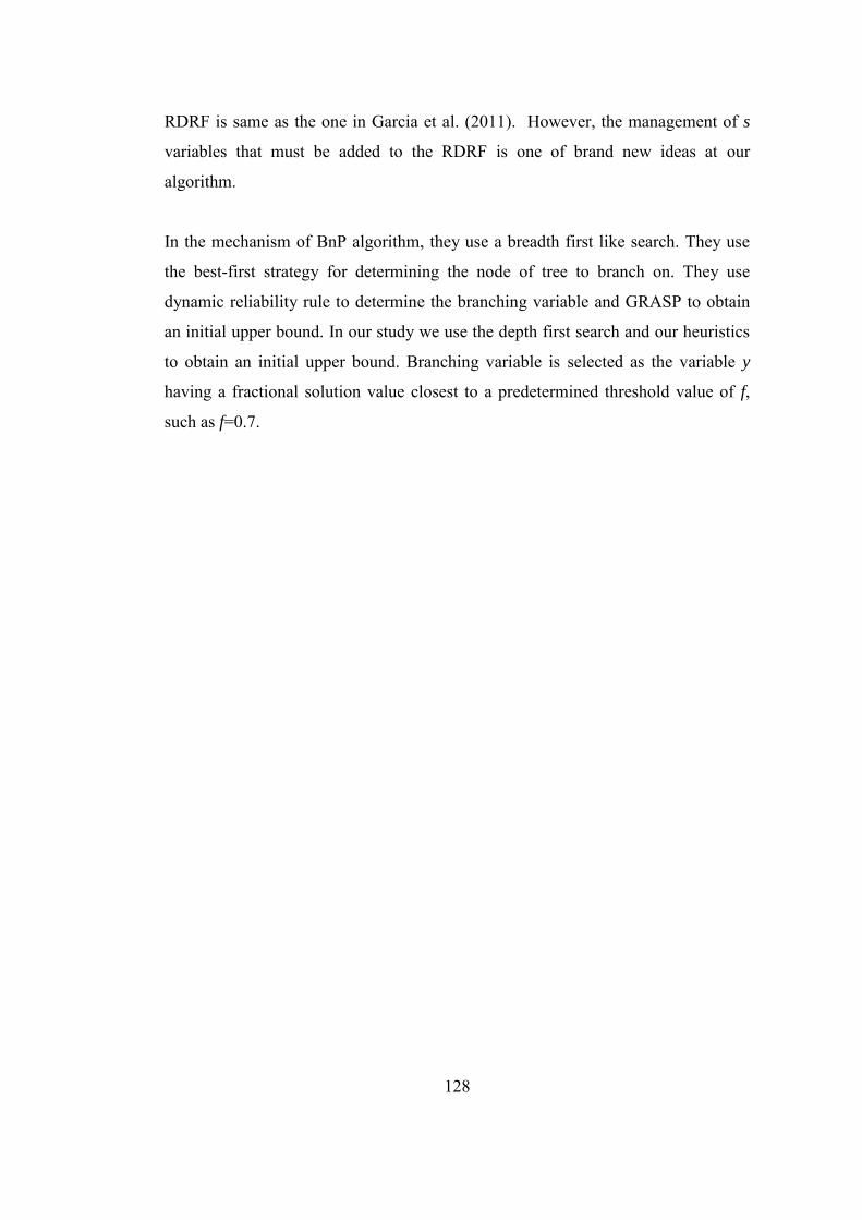
128

RDRF is same as the one in Garcia et al. (2011). However, the management of s

variables that must be added to the RDRF is one of brand new ideas at our

algorithm.

In the mechanism of BnP algorithm, they use a breadth first like search. They use

the best-first strategy for determining the node of tree to branch on. They use

dynamic reliability rule to determine the branching variable and GRASP to obtain

an initial upper bound. In our study we use the depth first search and our heuristics

to obtain an initial upper bound. Branching variable is selected as the variable y

having a fractional solution value closest to a predetermined threshold value of f,

such as f=0.7.

129

Fig

ure

B.1

: Flo

w c

hart

of th

e D

BnP

alg

orith

m

16

12

N

Y

Y

N

Y

N

Is

leve

l>0

?

Is

leve

l<=0

, an

d y D

leve

l=0

?

Is (l

evel

>0) a

nd

((yD

leve

l=0)

or

(LB l

evel>=

UB

)) ?

Dec

reas

e le

vel b

y 1

Rem

ove

the

y D

leve

l=1

(or 0

) co

ntra

int f

rom

RD

RF.

D

ecre

ase

leve

l by

1.

Rem

ove

the

prev

ious

ly

adde

d s

varia

bles

, it

sd itz

varia

bles

and

the

rela

ted

cons

train

ts a

fter t

his

leve

l fro

m R

DR

F. U

pdat

e sd

it

valu

es.

Add

the

y Dle

vel=

0 co

nstra

int t

o R

DR

F.

Incr

ease

leve

l by

1.

STO

P. R

epor

t the

UB

and

th

e be

st so

lutio

n.

6

13

11

14

15

17

Y

N

Y

Is th

ere

any

itsd it

z>0

or

(βit -

βjt )

> K

ji ?

Is in

tegr

ality

sa

tisfie

d?

UB

= ob

j. U

pdat

e th

e be

st so

lutio

n.

Is

obj.

<UB

?

N

Y

5

7

9

10

N

For a

ll (β

it - β

jt ) >

Kji a

dd

s jit t

o R

DR

F.

For a

ll itsd itz

>0 :

Incr

ease

sd

it b

y 1

Add

it

sd itz

Add

the

cons

train

t, 1,

itsd

iij

it

Ddj

jt

sd ity

z

to R

DR

F.

Y

N

Run

the

UB

heur

istic

. Sa

ve th

e so

lutio

n as

the

best

solu

tion

and

UB

valu

e.

Con

stru

ct th

e in

itial

LP

mod

el o

f RD

RF.

Use

on

ly fi

rst s

dit o

f it

sd itz

var

iabl

es a

nd n

o s

varia

ble.

Lev

el=0

.

Solv

e th

e R

DR

F

Is th

e so

lutio

n LP

op

t. ?

Cho

ose

the

clos

est 0

< y k

t <1

varia

ble

to

f as t

he b

ranc

hing

var

iabl

e.

LBle

vel =

obj.

Dle

vel =

y kt

Add

the

y kt=

1 co

nstra

int t

o R

DR

F.

Incr

ease

leve

l by

1

1

2

3

4

8

129

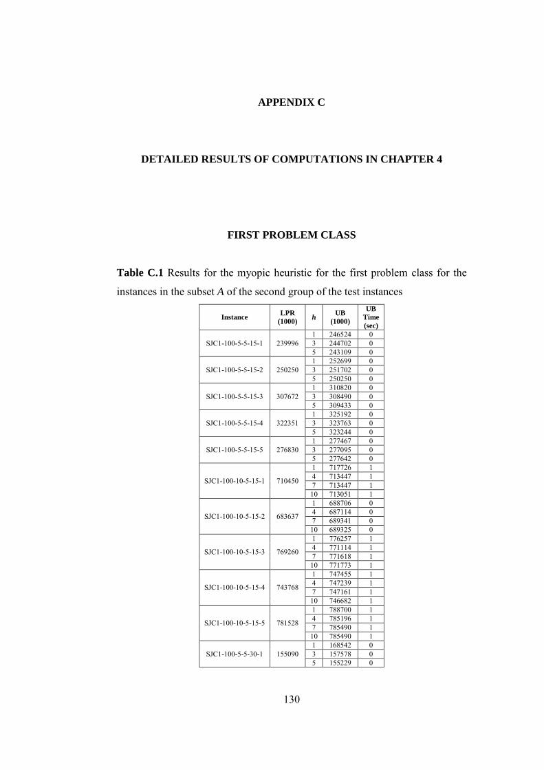
130

APPENDIX C

DETAILED RESULTS OF COMPUTATIONS IN CHAPTER 4

FIRST PROBLEM CLASS

Table C.1 Results for the myopic heuristic for the first problem class for the

instances in the subset A of the second group of the test instances

Instance LPR

(1000) h

UB

(1000)

UB

Time

(sec)

SJC1-100-5-5-15-1 239996 1 246524 0 3 244702 0 5 243109 0

SJC1-100-5-5-15-2 250250 1 252699 0 3 251702 0 5 250250 0

SJC1-100-5-5-15-3 307672 1 310820 0 3 308490 0 5 309433 0

SJC1-100-5-5-15-4 322351 1 325192 0 3 323763 0 5 323244 0

SJC1-100-5-5-15-5 276830 1 277467 0 3 277095 0 5 277642 0

SJC1-100-10-5-15-1 710450

1 717726 1 4 713447 1 7 713447 1

10 713051 1

SJC1-100-10-5-15-2 683637

1 688706 0 4 687114 0 7 689341 0

10 689325 0

SJC1-100-10-5-15-3 769260

1 776257 1 4 771114 1 7 771618 1

10 771773 1

SJC1-100-10-5-15-4 743768

1 747455 1 4 747239 1 7 747161 1

10 746682 1

SJC1-100-10-5-15-5 781528

1 788700 1 4 785196 1 7 785490 1

10 785490 1

SJC1-100-5-5-30-1 155090 1 168542 0 3 157578 0 5 155229 0

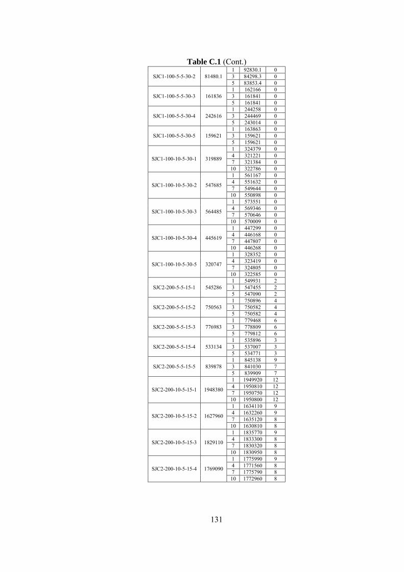
131

Table C.1 (Cont.)

SJC1-100-5-5-30-2 81480.1 1 92830.1 0 3 84298.3 0 5 83853.4 0

SJC1-100-5-5-30-3 161836 1 162166 0 3 161841 0 5 161841 0

SJC1-100-5-5-30-4 242616 1 244258 0 3 244469 0 5 243014 0

SJC1-100-5-5-30-5 159621 1 163863 0 3 159621 0 5 159621 0

SJC1-100-10-5-30-1 319889

1 324379 0 4 321221 0 7 321384 0

10 322786 0

SJC1-100-10-5-30-2 547685

1 561167 0 4 551632 0 7 549644 0

10 550898 0

SJC1-100-10-5-30-3 564485

1 573551 0 4 569346 0 7 570646 0

10 570009 0

SJC1-100-10-5-30-4 445619

1 447299 0 4 446168 0 7 447807 0

10 446268 0

SJC1-100-10-5-30-5 320747

1 328352 0 4 323419 0 7 324805 0

10 322585 0

SJC2-200-5-5-15-1 545286 1 549931 2 3 547455 2 5 547090 2

SJC2-200-5-5-15-2 750563 1 750896 4 3 750582 4 5 750582 4

SJC2-200-5-5-15-3 776983 1 779468 6 3 778809 6 5 779812 6

SJC2-200-5-5-15-4 533134 1 535896 3 3 537007 3 5 534771 3

SJC2-200-5-5-15-5 839878 1 845138 9 3 841030 7 5 839909 7

SJC2-200-10-5-15-1 1948380

1 1949920 12 4 1950810 12 7 1950750 12

10 1950800 12

SJC2-200-10-5-15-2 1627960

1 1634110 9 4 1632260 9 7 1635120 8

10 1630810 8

SJC2-200-10-5-15-3 1829110

1 1835770 9 4 1833300 8 7 1830320 8

10 1830950 8

SJC2-200-10-5-15-4 1769090

1 1775990 9 4 1771560 8 7 1775790 8

10 1772960 8

132

Table C.1 (Cont.)

SJC2-200-10-5-15-5 1575870

1 1581840 7 4 1579650 5 7 1579660 6

10 1578780 6

SJC2-200-5-5-30-1 707220 1 708498 5 3 710428 4 5 708155 4

SJC2-200-5-5-30-2 441991 1 443968 2 3 445041 2 5 445466 1

SJC2-200-5-5-30-3 407197 1 409632 1 3 407769 1 5 407197 1

SJC2-200-5-5-30-4 743608 1 746242 6 3 746007 6 5 745225 6

SJC2-200-5-5-30-5 626238 1 626761 4 3 627842 3 5 626800 3

SJC2-200-10-5-30-1 1636560

1 1644130 8 4 1640550 8 7 1642810 8

10 1642980 8

SJC2-200-10-5-30-2 1286130

1 1291830 4 4 1287810 4 7 1289520 4

10 1291660 5

SJC2-200-10-5-30-3 1179740

1 1185670 4 4 1187300 4 7 1186890 4

10 1187490 3

SJC2-200-10-5-30-4 1153260

1 1162040 4 4 1156980 4 7 1156060 3

10 1156160 3

SJC2-200-10-5-30-5 1030060

1 1039390 2 4 1035460 2 7 1040130 2

10 1035300 3

SJC3-300-5-5-15-1 1104020 1 1106510 24 3 1110450 23 5 1109050 18

SJC3-300-5-5-15-2 967640 1 971235 19 3 972705 19 5 974207 18

SJC3-300-5-5-15-3 1216780 1 1217690 32 3 1217510 30 5 1218980 29

SJC3-300-5-5-15-4 1325290 1 1326590 41 3 1330120 38 5 1330970 33

SJC3-300-5-5-15-5 1225150 1 1228380 38 3 1225960 36 5 1226850 29

SJC3-300-10-5-15-1 2982250

1 2988990 59 4 2984800 61 7 2984220 58

10 2985360 48

SJC3-300-10-5-15-2 2661330

1 2672780 41 4 2666420 41 7 2665840 40

10 2672390 41

SJC3-300-10-5-15-3 3001280

1 3005970 54 4 3004960 54 7 3005440 51

10 3003550 50

133

Table C.1 (Cont.)

SJC3-300-10-5-15-4 3287360

1 3296360 65 4 3291810 66 7 3288150 59

10 3289590 67

SJC3-300-10-5-15-5 2792670

1 2796340 40 4 2796560 36 7 2795820 34

10 2796160 36

SJC3-300-5-5-30-1 577993 1 583570 4 3 582611 4 5 581549 4

SJC3-300-5-5-30-2 603527 1 609794 5 3 612952 5 5 610644 3

SJC3-300-5-5-30-3 786640 1 789264 9 3 787978 8 5 789735 8

SJC3-300-5-5-30-4 769035 1 781016 14 3 772375 12 5 777242 8

SJC3-300-5-5-30-5 956705 1 968093 25 3 961459 25 5 960126 22

SJC3-300-10-5-30-1 2286980

1 2292720 31 4 2290220 30 7 2299110 29

10 2298250 23

SJC3-300-10-5-30-2 2014790

1 2021110 23 4 2018370 24 7 2019950 25

10 2021090 30

SJC3-300-10-5-30-3 2462820

1 2468030 34 4 2467770 33 7 2466080 32

10 2467280 36

SJC3-300-10-5-30-4 2112250

1 2122170 27 4 2121040 27 7 2116560 24

10 2116030 25

SJC3-300-10-5-30-5 1695500

1 1704330 13 4 1703020 13 7 1703560 12

10 1701830 11

134

Table C.2 Results for the progressive heuristics for the first problem class for

the instances in the subset A of the second group of the test instances

Instance LPR

(1000) h

Progressive-1 Progressive-2

UB

(1000)

UB

Time

(sec)

UB

(1000)

UB

Time

(sec)

SJC1-100-5-5-15-1 239996 1 256061 0 257625 0 T* 248456 0 252511 0

SJC1-100-5-5-15-2 250250 1 261363 0 279087 0 T* 271713 0 273360 0

SJC1-100-5-5-15-3 307672 1 326257 0 331730 0 T* 322957 0 334958 0

SJC1-100-5-5-15-4 322351 1 341413 0 334226 0 T* 361217 0 366707 0

SJC1-100-5-5-15-5 276830 1 300361 0 290959 0 T* 303263 0 305978 0

SJC1-100-10-5-15-1 710450 1 744914 0 761553 0 T* 758701 0 750232 1

SJC1-100-10-5-15-2 683637 1 738309 0 741972 0 T* 801409 0 774831 1

SJC1-100-10-5-15-3 769260 1 818043 0 812174 0 T* 780896 0 782762 1

SJC1-100-10-5-15-4 743768 1 807516 0 805099 0 T* 780320 0 771543 1

SJC1-100-10-5-15-5 781528 1 820077 0 812245 0 T* 859165 0 859165 1

SJC1-100-5-5-30-1 155090 1 166110 0 165993 0 T* 274287 0 274298 0

SJC1-100-5-5-30-2 81480.1 1 111472 0 91647.2 0 T* 85970.4 0 88380.3 0

SJC1-100-5-5-30-3 161836 1 181795 0 176227 0 T* 181855 0 176118 0

SJC1-100-5-5-30-4 242616 1 310110 0 253647 0 T* 287069 0 287069 0

SJC1-100-5-5-30-5 159621 1 165224 0 173484 0 T* 230019 0 231525 0

SJC1-100-10-5-30-1 319889 1 476279 0 364222 0 T* 351189 0 356418 0

SJC1-100-10-5-30-2 547685 1 588894 0 587361 0 T* 713853 0 681699 0

SJC1-100-10-5-30-3 564485 1 614636 0 602661 0 T* 646395 0 589094 0

SJC1-100-10-5-30-4 445619 1 491822 0 499196 0 T* 493478 0 484840 0

SJC1-100-10-5-30-5 320747 1 338038 0 349475 0 T* 388990 0 358428 0

SJC2-200-5-5-15-1 545286 1 566968 1 564539 2 T* 698165 2 699561 6

SJC2-200-5-5-15-2 750563 1 789367 5 791668 6 T* 805866 10 805109 11

SJC2-200-5-5-15-3 776983 1 804348 4 803903 6 T* 846824 8 837896 15

SJC2-200-5-5-15-4 533134 1 576338 2 584099 4 T* 570445 5 578795 9

SJC2-200-5-5-15-5 839878 1 876962 6 862601 10 T* 922491 12 928521 20

SJC2-200-10-5-15-1 1948380 1 2078330 7 2088890 10 T* 2079120 13 2118420 29

SJC2-200-10-5-15-2 1627960 1 1717970 4 1716510 5 T* 1720350 10 1728540 15

SJC2-200-10-5-15-3 1829110 1 1948230 6 1948230 7 T* 1952580 15 1923920 16

SJC2-200-10-5-15-4 1769090 1 1856320 5 1843000 7 T* 1883900 15 1864420 20

SJC2-200-10-5-15-5 1575870 1 1681290 1 1634400 4 T* 1661050 5 1663260 9

135

Table C.2 (Cont.) SJC2-200-5-5-30-1 707220 1 729886 4 730177 4

T* 865128 10 813023 10

SJC2-200-5-5-30-2 441991 1 471115 2 466105 2 T* 512766 3 493982 4

SJC2-200-5-5-30-3 407197 1 451521 2 446130 4 T* 438981 2 426839 6

SJC2-200-5-5-30-4 743608 1 776174 5 783878 7 T* 832786 12 835549 14

SJC2-200-5-5-30-5 626238 1 669047 5 656677 8 T* 710315 12 710315 10

SJC2-200-10-5-30-1 1636560 1 1740210 8 1743240 9 T* 1860490 21 1862190 18

SJC2-200-10-5-30-2 1286130 1 1350940 3 1401010 7 T* 1399570 14 1375210 17

SJC2-200-10-5-30-3 1179740 1 1267400 3 1299980 6 T* 1277790 6 1240470 14

SJC2-200-10-5-30-4 1153260 1 1209380 4 1208150 4 T* 1555080 4 1555810 5

SJC2-200-10-5-30-5 1030060 1 1128640 2 1102620 4 T* 1137810 4 1131500 6

SJC3-300-5-5-15-1 1104020 1 1132810 23 1151370 25 T* 1148910 34 1148910 51

SJC3-300-5-5-15-2 967640 1 1037030 11 1010560 30 T* 1001500 29 1018580 69

SJC3-300-5-5-15-3 1216780 1 1236930 31 1236930 32 T* 1243690 46 1243690 69

SJC3-300-5-5-15-4 1325290 1 1358090 37 1369190 36 T* 1397150 37 1399370 47

SJC3-300-5-5-15-5 1225150 1 1263330 43 1257180 46 T* 1315840 46 1323490 59

SJC3-300-10-5-15-1 2982250 1 3102980 35 3116530 46 T* 3526200 53 3456630 89

SJC3-300-10-5-15-2 2661330 1 2810590 35 2789170 49 T* 2790590 53 2789930 97

SJC3-300-10-5-15-3 3001280 1 3096470 40 3093040 38 T* 3103080 74 3119050 81

SJC3-300-10-5-15-4 3287360 1 3437250 45 3423730 55 T* 3459320 76 3465090 100

SJC3-300-10-5-15-5 2792670 1 2903540 18 2877900 45 T* 2912610 45 2933510 76

SJC3-300-5-5-30-1 577993 1 596280 3 619429 4 T* 605070 5 612988 11

SJC3-300-5-5-30-2 603527 1 664316 3 635833 7 T* 643792 10 647095 19

SJC3-300-5-5-30-3 786640 1 814533 7 812308 22 T* 852779 17 870398 29

SJC3-300-5-5-30-4 769035 1 805157 17 807294 20 T* 799702 12 800837 23

SJC3-300-5-5-30-5 956705 1 985224 35 982458 36 T* 1049370 43 1051310 35

SJC3-300-10-5-30-1 2286980 1 2433430 33 2424680 43 T* 2499250 46 2446540 74

SJC3-300-10-5-30-2 2014790 1 2126600 27 2107850 36 T* 2360700 46 2352080 45

SJC3-300-10-5-30-3 2462820 1 2558620 32 2548960 53 T* 2587750 57 2569360 77

SJC3-300-10-5-30-4 2112250 1 2194440 11 2201510 19 T* 2356900 23 2209960 47

SJC3-300-10-5-30-5 1695500 1 1784690 9 1813400 13 T* 1914200 19 1846480 30

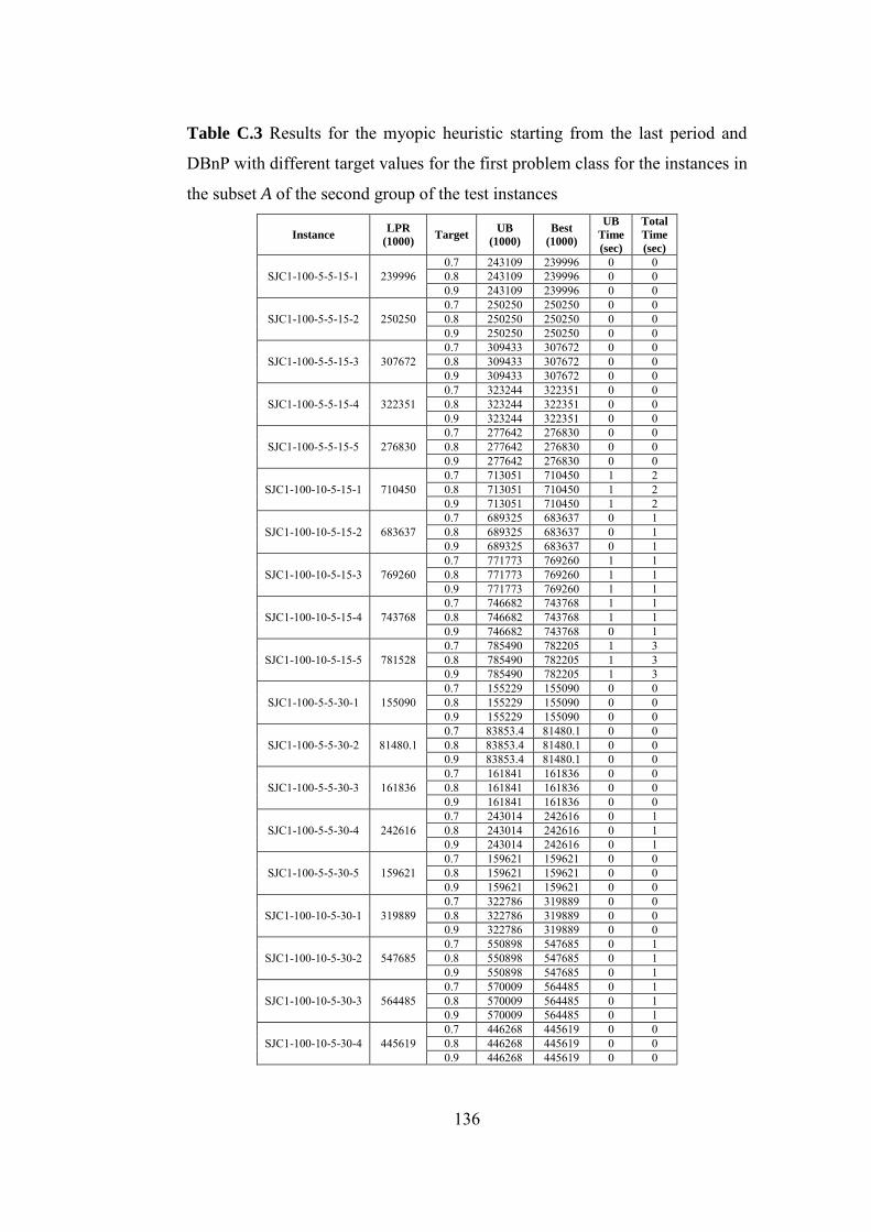
136

Table C.3 Results for the myopic heuristic starting from the last period and

DBnP with different target values for the first problem class for the instances in

the subset A of the second group of the test instances

Instance LPR

(1000) Target

UB

(1000)

Best

(1000)

UB

Time

(sec)

Total

Time

(sec)

SJC1-100-5-5-15-1 239996 0.7 243109 239996 0 0 0.8 243109 239996 0 0 0.9 243109 239996 0 0

SJC1-100-5-5-15-2 250250 0.7 250250 250250 0 0 0.8 250250 250250 0 0 0.9 250250 250250 0 0

SJC1-100-5-5-15-3 307672 0.7 309433 307672 0 0 0.8 309433 307672 0 0 0.9 309433 307672 0 0

SJC1-100-5-5-15-4 322351 0.7 323244 322351 0 0 0.8 323244 322351 0 0 0.9 323244 322351 0 0

SJC1-100-5-5-15-5 276830 0.7 277642 276830 0 0 0.8 277642 276830 0 0 0.9 277642 276830 0 0

SJC1-100-10-5-15-1 710450 0.7 713051 710450 1 2 0.8 713051 710450 1 2 0.9 713051 710450 1 2

SJC1-100-10-5-15-2 683637 0.7 689325 683637 0 1 0.8 689325 683637 0 1 0.9 689325 683637 0 1

SJC1-100-10-5-15-3 769260 0.7 771773 769260 1 1 0.8 771773 769260 1 1 0.9 771773 769260 1 1

SJC1-100-10-5-15-4 743768 0.7 746682 743768 1 1 0.8 746682 743768 1 1 0.9 746682 743768 0 1

SJC1-100-10-5-15-5 781528 0.7 785490 782205 1 3 0.8 785490 782205 1 3 0.9 785490 782205 1 3

SJC1-100-5-5-30-1 155090 0.7 155229 155090 0 0 0.8 155229 155090 0 0 0.9 155229 155090 0 0

SJC1-100-5-5-30-2 81480.1 0.7 83853.4 81480.1 0 0 0.8 83853.4 81480.1 0 0 0.9 83853.4 81480.1 0 0

SJC1-100-5-5-30-3 161836 0.7 161841 161836 0 0 0.8 161841 161836 0 0 0.9 161841 161836 0 0

SJC1-100-5-5-30-4 242616 0.7 243014 242616 0 1 0.8 243014 242616 0 1 0.9 243014 242616 0 1

SJC1-100-5-5-30-5 159621 0.7 159621 159621 0 0 0.8 159621 159621 0 0 0.9 159621 159621 0 0

SJC1-100-10-5-30-1 319889 0.7 322786 319889 0 0 0.8 322786 319889 0 0 0.9 322786 319889 0 0

SJC1-100-10-5-30-2 547685 0.7 550898 547685 0 1 0.8 550898 547685 0 1 0.9 550898 547685 0 1

SJC1-100-10-5-30-3 564485 0.7 570009 564485 0 1 0.8 570009 564485 0 1 0.9 570009 564485 0 1

SJC1-100-10-5-30-4 445619 0.7 446268 445619 0 0 0.8 446268 445619 0 0 0.9 446268 445619 0 0

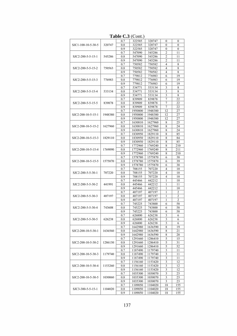
137

Table C.3 (Cont.)

SJC1-100-10-5-30-5 320747 0.7 322585 320747 0 0 0.8 322585 320747 0 0 0.9 322585 320747 0 0

SJC2-200-5-5-15-1 545286 0.7 547090 545286 2 11 0.8 547090 545286 2 11 0.9 547090 545286 2 11

SJC2-200-5-5-15-2 750563 0.7 750582 750582 4 8 0.8 750582 750582 4 8 0.9 750582 750582 4 8

SJC2-200-5-5-15-3 776983 0.7 779812 776983 6 19 0.8 779812 776983 6 19 0.9 779812 776983 6 19

SJC2-200-5-5-15-4 533134 0.7 534771 533134 3 8 0.8 534771 533134 3 8 0.9 534771 533134 3 8

SJC2-200-5-5-15-5 839878 0.7 839909 839878 7 22 0.8 839909 839878 7 22 0.9 839909 839878 7 22

SJC2-200-10-5-15-1 1948380 0.7 1950800 1948380 12 27 0.8 1950800 1948380 12 27 0.9 1950800 1948380 12 27

SJC2-200-10-5-15-2 1627960 0.7 1630810 1627960 8 25 0.8 1630810 1627960 8 24 0.9 1630810 1627960 8 24

SJC2-200-10-5-15-3 1829110 0.7 1830950 1829110 8 85 0.8 1830950 1829110 8 84 0.9 1830950 1829110 8 85

SJC2-200-10-5-15-4 1769090 0.7 1772960 1769240 8 210 0.8 1772960 1769240 8 211 0.9 1772960 1769240 8 210

SJC2-200-10-5-15-5 1575870 0.7 1578780 1575870 6 38 0.8 1578780 1575870 6 39 0.9 1578780 1575870 6 38

SJC2-200-5-5-30-1 707220 0.7 708155 707220 4 10 0.8 708155 707220 4 10 0.9 708155 707220 4 10

SJC2-200-5-5-30-2 441991 0.7 445466 442212 1 10 0.8 445466 442212 1 11 0.9 445466 442212 1 10

SJC2-200-5-5-30-3 407197 0.7 407197 407197 1 2 0.8 407197 407197 1 2 0.9 407197 407197 1 2

SJC2-200-5-5-30-4 743608 0.7 745225 743800 6 58 0.8 745225 743800 6 58 0.9 745225 743800 6 58

SJC2-200-5-5-30-5 626238 0.7 626800 626238 3 6 0.8 626800 626238 3 6 0.9 626800 626238 3 6

SJC2-200-10-5-30-1 1636560 0.7 1642980 1636590 8 19 0.8 1642980 1636590 8 21 0.9 1642980 1636590 8 20

SJC2-200-10-5-30-2 1286130 0.7 1291660 1286410 5 15 0.8 1291660 1286410 5 31 0.9 1291660 1286410 5 52

SJC2-200-10-5-30-3 1179740 0.7 1187490 1179740 3 11 0.8 1187490 1179740 3 11 0.9 1187490 1179740 3 11

SJC2-200-10-5-30-4 1153260 0.7 1156160 1153420 3 12 0.8 1156160 1153420 3 12 0.9 1156160 1153420 3 12

SJC2-200-10-5-30-5 1030060 0.7 1035300 1030070 3 23 0.8 1035300 1030070 3 23 0.9 1035300 1030070 3 23

SJC3-300-5-5-15-1 1104020 0.7 1109050 1104020 18 155 0.8 1109050 1104020 18 155 0.9 1109050 1104020 18 155

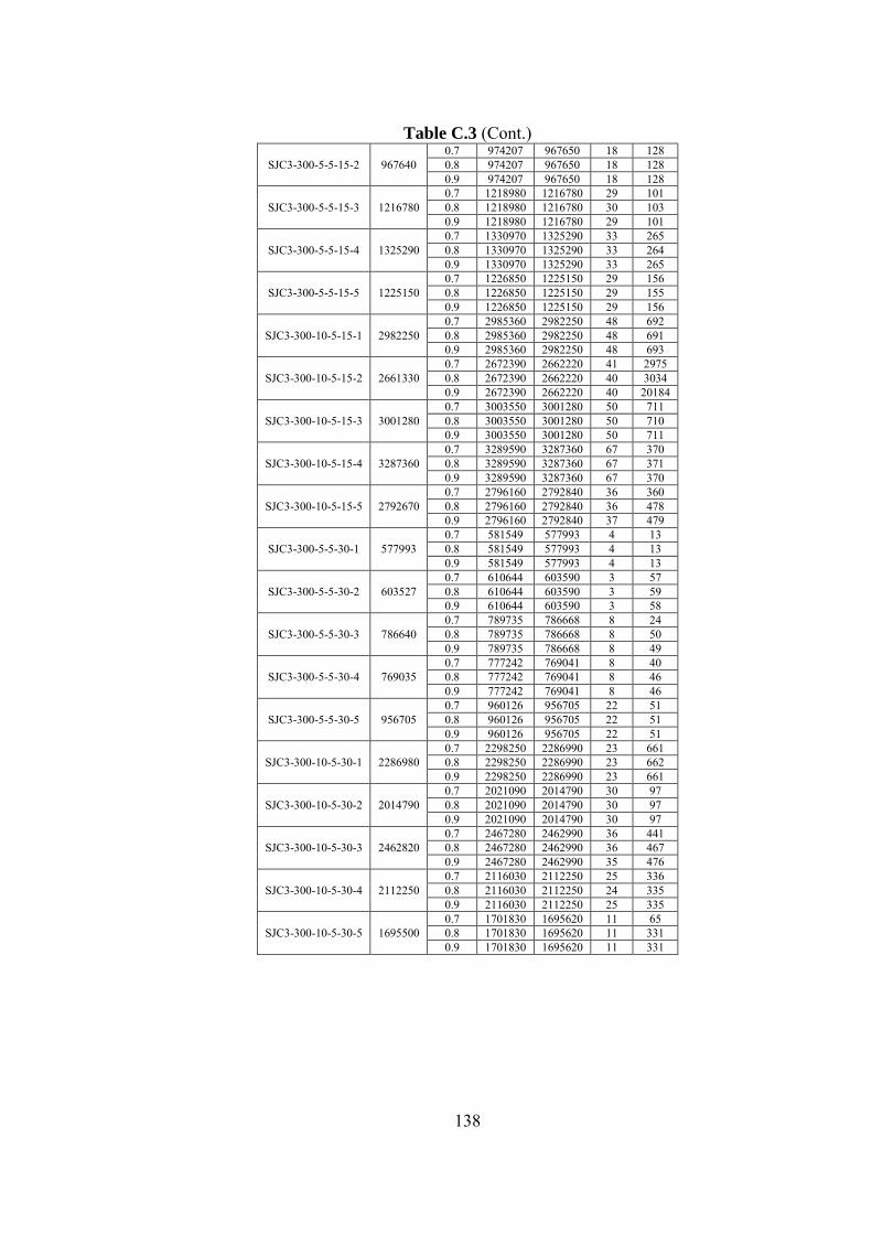
138

Table C.3 (Cont.)

SJC3-300-5-5-15-2 967640 0.7 974207 967650 18 128 0.8 974207 967650 18 128 0.9 974207 967650 18 128

SJC3-300-5-5-15-3 1216780 0.7 1218980 1216780 29 101 0.8 1218980 1216780 30 103 0.9 1218980 1216780 29 101

SJC3-300-5-5-15-4 1325290 0.7 1330970 1325290 33 265 0.8 1330970 1325290 33 264 0.9 1330970 1325290 33 265

SJC3-300-5-5-15-5 1225150 0.7 1226850 1225150 29 156 0.8 1226850 1225150 29 155 0.9 1226850 1225150 29 156

SJC3-300-10-5-15-1 2982250 0.7 2985360 2982250 48 692 0.8 2985360 2982250 48 691 0.9 2985360 2982250 48 693

SJC3-300-10-5-15-2 2661330 0.7 2672390 2662220 41 2975 0.8 2672390 2662220 40 3034 0.9 2672390 2662220 40 20184

SJC3-300-10-5-15-3 3001280 0.7 3003550 3001280 50 711 0.8 3003550 3001280 50 710 0.9 3003550 3001280 50 711

SJC3-300-10-5-15-4 3287360 0.7 3289590 3287360 67 370 0.8 3289590 3287360 67 371 0.9 3289590 3287360 67 370

SJC3-300-10-5-15-5 2792670 0.7 2796160 2792840 36 360 0.8 2796160 2792840 36 478 0.9 2796160 2792840 37 479

SJC3-300-5-5-30-1 577993 0.7 581549 577993 4 13 0.8 581549 577993 4 13 0.9 581549 577993 4 13

SJC3-300-5-5-30-2 603527 0.7 610644 603590 3 57 0.8 610644 603590 3 59 0.9 610644 603590 3 58

SJC3-300-5-5-30-3 786640 0.7 789735 786668 8 24 0.8 789735 786668 8 50 0.9 789735 786668 8 49

SJC3-300-5-5-30-4 769035 0.7 777242 769041 8 40 0.8 777242 769041 8 46 0.9 777242 769041 8 46

SJC3-300-5-5-30-5 956705 0.7 960126 956705 22 51 0.8 960126 956705 22 51 0.9 960126 956705 22 51

SJC3-300-10-5-30-1 2286980 0.7 2298250 2286990 23 661 0.8 2298250 2286990 23 662 0.9 2298250 2286990 23 661

SJC3-300-10-5-30-2 2014790 0.7 2021090 2014790 30 97 0.8 2021090 2014790 30 97 0.9 2021090 2014790 30 97

SJC3-300-10-5-30-3 2462820 0.7 2467280 2462990 36 441 0.8 2467280 2462990 36 467 0.9 2467280 2462990 35 476

SJC3-300-10-5-30-4 2112250 0.7 2116030 2112250 25 336 0.8 2116030 2112250 24 335 0.9 2116030 2112250 25 335

SJC3-300-10-5-30-5 1695500 0.7 1701830 1695620 11 65 0.8 1701830 1695620 11 331 0.9 1701830 1695620 11 331

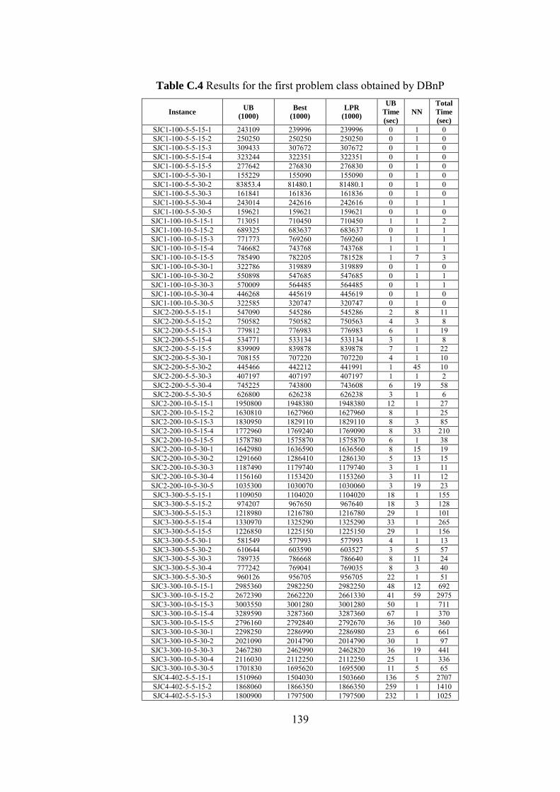
139

Table C.4 Results for the first problem class obtained by DBnP

Instance UB

(1000)

Best

(1000)

LPR

(1000)

UB

Time

(sec)

NN

Total

Time

(sec)

SJC1-100-5-5-15-1 243109 239996 239996 0 1 0 SJC1-100-5-5-15-2 250250 250250 250250 0 1 0 SJC1-100-5-5-15-3 309433 307672 307672 0 1 0 SJC1-100-5-5-15-4 323244 322351 322351 0 1 0 SJC1-100-5-5-15-5 277642 276830 276830 0 1 0 SJC1-100-5-5-30-1 155229 155090 155090 0 1 0 SJC1-100-5-5-30-2 83853.4 81480.1 81480.1 0 1 0 SJC1-100-5-5-30-3 161841 161836 161836 0 1 0 SJC1-100-5-5-30-4 243014 242616 242616 0 1 1 SJC1-100-5-5-30-5 159621 159621 159621 0 1 0 SJC1-100-10-5-15-1 713051 710450 710450 1 1 2 SJC1-100-10-5-15-2 689325 683637 683637 0 1 1 SJC1-100-10-5-15-3 771773 769260 769260 1 1 1 SJC1-100-10-5-15-4 746682 743768 743768 1 1 1 SJC1-100-10-5-15-5 785490 782205 781528 1 7 3 SJC1-100-10-5-30-1 322786 319889 319889 0 1 0 SJC1-100-10-5-30-2 550898 547685 547685 0 1 1 SJC1-100-10-5-30-3 570009 564485 564485 0 1 1 SJC1-100-10-5-30-4 446268 445619 445619 0 1 0 SJC1-100-10-5-30-5 322585 320747 320747 0 1 0 SJC2-200-5-5-15-1 547090 545286 545286 2 8 11 SJC2-200-5-5-15-2 750582 750582 750563 4 3 8 SJC2-200-5-5-15-3 779812 776983 776983 6 1 19 SJC2-200-5-5-15-4 534771 533134 533134 3 1 8 SJC2-200-5-5-15-5 839909 839878 839878 7 1 22 SJC2-200-5-5-30-1 708155 707220 707220 4 1 10 SJC2-200-5-5-30-2 445466 442212 441991 1 45 10 SJC2-200-5-5-30-3 407197 407197 407197 1 1 2 SJC2-200-5-5-30-4 745225 743800 743608 6 19 58 SJC2-200-5-5-30-5 626800 626238 626238 3 1 6 SJC2-200-10-5-15-1 1950800 1948380 1948380 12 1 27 SJC2-200-10-5-15-2 1630810 1627960 1627960 8 1 25 SJC2-200-10-5-15-3 1830950 1829110 1829110 8 3 85 SJC2-200-10-5-15-4 1772960 1769240 1769090 8 33 210 SJC2-200-10-5-15-5 1578780 1575870 1575870 6 1 38 SJC2-200-10-5-30-1 1642980 1636590 1636560 8 15 19 SJC2-200-10-5-30-2 1291660 1286410 1286130 5 13 15 SJC2-200-10-5-30-3 1187490 1179740 1179740 3 1 11 SJC2-200-10-5-30-4 1156160 1153420 1153260 3 11 12 SJC2-200-10-5-30-5 1035300 1030070 1030060 3 19 23 SJC3-300-5-5-15-1 1109050 1104020 1104020 18 1 155 SJC3-300-5-5-15-2 974207 967650 967640 18 3 128 SJC3-300-5-5-15-3 1218980 1216780 1216780 29 1 101 SJC3-300-5-5-15-4 1330970 1325290 1325290 33 1 265 SJC3-300-5-5-15-5 1226850 1225150 1225150 29 1 156 SJC3-300-5-5-30-1 581549 577993 577993 4 1 13 SJC3-300-5-5-30-2 610644 603590 603527 3 5 57 SJC3-300-5-5-30-3 789735 786668 786640 8 11 24 SJC3-300-5-5-30-4 777242 769041 769035 8 3 40 SJC3-300-5-5-30-5 960126 956705 956705 22 1 51 SJC3-300-10-5-15-1 2985360 2982250 2982250 48 12 692 SJC3-300-10-5-15-2 2672390 2662220 2661330 41 59 2975 SJC3-300-10-5-15-3 3003550 3001280 3001280 50 1 711 SJC3-300-10-5-15-4 3289590 3287360 3287360 67 1 370 SJC3-300-10-5-15-5 2796160 2792840 2792670 36 10 360 SJC3-300-10-5-30-1 2298250 2286990 2286980 23 6 661 SJC3-300-10-5-30-2 2021090 2014790 2014790 30 1 97 SJC3-300-10-5-30-3 2467280 2462990 2462820 36 19 441 SJC3-300-10-5-30-4 2116030 2112250 2112250 25 1 336 SJC3-300-10-5-30-5 1701830 1695620 1695500 11 5 65 SJC4-402-5-5-15-1 1510960 1504030 1503660 136 5 2707 SJC4-402-5-5-15-2 1868060 1866350 1866350 259 1 1410 SJC4-402-5-5-15-3 1800900 1797500 1797500 232 1 1025

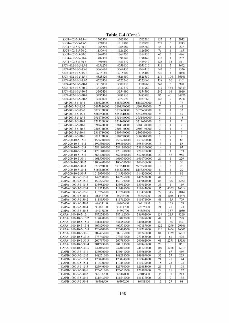
140

Table C.4 (Cont.) SJC4-402-5-5-15-4 1705570 1702900 1702580 157 7 2032 SJC4-402-5-5-15-5 1721030 1719800 1719790 277 5 1245 SJC4-402-5-5-30-1 1068210 1065680 1065680 56 1 227 SJC4-402-5-5-30-2 1130940 1126200 1126200 76 1 165 SJC4-402-5-5-30-3 1269070 1264750 1264730 67 3 496 SJC4-402-5-5-30-4 1402390 1398140 1398140 135 1 232 SJC4-402-5-5-30-5 1491980 1489310 1489240 125 15 511 SJC4-402-10-5-15-1 4056270 4051010 4051010 316 5 3692 SJC4-402-10-5-15-2 5067660 5064430 5064410 543 5 5336 SJC4-402-10-5-15-3 3718160 3715100 3715100 220 4 5068 SJC4-402-10-5-15-4 4828820 4826850 4825850 216 104 36161 SJC4-402-10-5-15-5 4526950 4525240 4525060 358 10 6101 SJC4-402-10-5-30-1 3316030 3309010 3308960 242 3 970 SJC4-402-10-5-30-2 3337080 3332510 3331960 117 444 36339 SJC4-402-10-5-30-3 3562430 3554690 3554590 242 16 1919 SJC4-402-10-5-30-4 3496360 3486530 3485790 86 401 34276 SJC4-402-10-5-30-5 3080070 3077690 3077660 148 7 1568

AP-200-5-5-15-1 6205220000 6187870000 6187870000 11 1 76 AP-200-5-5-15-2 5607840000 5604590000 5604590000 7 1 41 AP-200-5-5-15-3 5077120000 5076630000 5076630000 8 1 33 AP-200-5-5-15-4 5860900000 5857510000 5857280000 9 3 47 AP-200-5-5-15-5 3951740000 3951460000 3951460000 3 1 18 AP-200-5-5-30-1 3217260000 3214620000 3214620000 2 1 7 AP-200-5-5-30-2 3289450000 3284170000 3284170000 3 1 7 AP-200-5-5-30-3 2505310000 2503140000 2503140000 2 1 4 AP-200-5-5-30-4 3314780000 3307490000 3307490000 2 1 7 AP-200-5-5-30-5 3013130000 3009720000 3009310000 1 9 8 AP-200-10-5-15-1 14536300000 14535200000 14535200000 16 1 88 AP-200-10-5-15-2 11995500000 11988100000 11988100000 13 1 88 AP-200-10-5-15-3 12891800000 12891100000 12891100000 14 1 97 AP-200-10-5-15-4 14201400000 14201200000 14201200000 18 1 153 AP-200-10-5-15-5 15633700000 15625600000 15622000000 23 47 956 AP-200-10-5-30-1 16615000000 16610700000 16610700000 26 1 229 AP-200-10-5-30-2 11006900000 11006500000 11006300000 10 3 50 AP-200-10-5-30-3 9777930000 9775510000 9775500000 10 3 26 AP-200-10-5-30-4 8160810000 8153200000 8153200000 8 1 29 AP-200-10-5-30-5 10159300000 10145500000 10144300000 8 9 86

CAPA-1000-5-5-15-1 148280000 148276000 148242000 44 7 151 CAPA-1000-5-5-15-2 150225000 150179000 149981000 86 725 8232 CAPA-1000-5-5-15-3 133982000 133952000 133952000 33 1 119 CAPA-1000-5-5-15-4 119525000 119486000 119047000 57 4105 36014 CAPA-1000-5-5-15-5 113766000 113704000 113477000 22 345 1844 CAPA-1000-5-5-30-1 86142700 85943400 85654600 21 3035 14471 CAPA-1000-5-5-30-2 111895000 111762000 111671000 41 135 709 CAPA-1000-5-5-30-3 66854100 66746400 66710800 5 155 159 CAPA-1000-5-5-30-4 93185100 93114700 92875300 21 21 123 CAPA-1000-5-5-30-5 84918800 84799700 84555600 14 357 1030 CAPA-1000-10-5-15-1 387224000 387162000 386902000 134 215 4269 CAPA-1000-10-5-15-2 317080000 317047000 317047000 44 1 288 CAPA-1000-10-5-15-3 341414000 341356000 341061000 80 165 3471 CAPA-1000-10-5-15-4 407829000 407574000 407187000 122 1299 29566 CAPA-1000-10-5-15-5 320630000 320464000 319718000 110 3404 36002 CAPA-1000-10-5-30-1 309475000 309125000 308745000 84 3329 36018 CAPA-1000-10-5-30-2 273748000 273597000 273453000 44 61 495 CAPA-1000-10-5-30-3 260797000 260783000 260662000 61 2271 15536 CAPA-1000-10-5-30-4 201243000 201103000 200940000 20 101 851 CAPA-1000-10-5-30-5 242045000 242045000 241126000 107 3218 36019 CAPB-1000-5-5-15-1 136096000 136041000 135961000 33 67 469 CAPB-1000-5-5-15-2 148221000 148218000 148099000 35 35 253 CAPB-1000-5-5-15-3 120090000 120024000 119944000 21 21 144 CAPB-1000-5-5-15-4 110500000 110461000 110339000 15 23 173 CAPB-1000-5-5-15-5 125946000 125790000 125683000 29 5 108 CAPB-1000-5-5-30-1 126651000 126651000 126595000 28 11 132 CAPB-1000-5-5-30-2 92673200 92587000 92405400 35 37 213 CAPB-1000-5-5-30-3 131543000 131543000 131437000 29 9 135 CAPB-1000-5-5-30-4 86508500 86507200 86481800 13 27 98

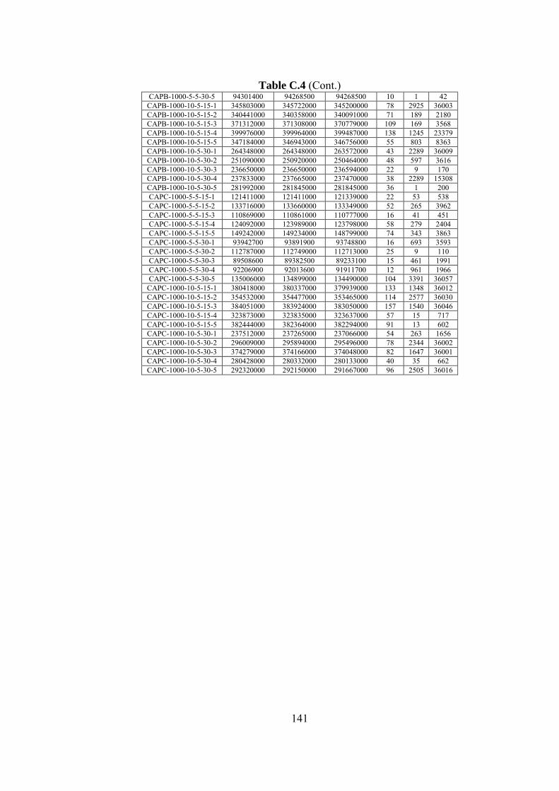
141

Table C.4 (Cont.) CAPB-1000-5-5-30-5 94301400 94268500 94268500 10 1 42

CAPB-1000-10-5-15-1 345803000 345722000 345200000 78 2925 36003 CAPB-1000-10-5-15-2 340441000 340358000 340091000 71 189 2180 CAPB-1000-10-5-15-3 371312000 371308000 370779000 109 169 3568 CAPB-1000-10-5-15-4 399976000 399964000 399487000 138 1245 23379 CAPB-1000-10-5-15-5 347184000 346943000 346756000 55 803 8363 CAPB-1000-10-5-30-1 264348000 264348000 263572000 43 2289 36009 CAPB-1000-10-5-30-2 251090000 250920000 250464000 48 597 3616 CAPB-1000-10-5-30-3 236650000 236650000 236594000 22 9 170 CAPB-1000-10-5-30-4 237833000 237665000 237470000 38 2289 15308 CAPB-1000-10-5-30-5 281992000 281845000 281845000 36 1 200 CAPC-1000-5-5-15-1 121411000 121411000 121339000 22 53 538 CAPC-1000-5-5-15-2 133716000 133660000 133349000 52 265 3962 CAPC-1000-5-5-15-3 110869000 110861000 110777000 16 41 451 CAPC-1000-5-5-15-4 124092000 123989000 123798000 58 279 2404 CAPC-1000-5-5-15-5 149242000 149234000 148799000 74 343 3863 CAPC-1000-5-5-30-1 93942700 93891900 93748800 16 693 3593 CAPC-1000-5-5-30-2 112787000 112749000 112713000 25 9 110 CAPC-1000-5-5-30-3 89508600 89382500 89233100 15 461 1991 CAPC-1000-5-5-30-4 92206900 92013600 91911700 12 961 1966 CAPC-1000-5-5-30-5 135006000 134899000 134490000 104 3391 36057

CAPC-1000-10-5-15-1 380418000 380337000 379939000 133 1348 36012 CAPC-1000-10-5-15-2 354532000 354477000 353465000 114 2577 36030 CAPC-1000-10-5-15-3 384051000 383924000 383050000 157 1540 36046 CAPC-1000-10-5-15-4 323873000 323835000 323637000 57 15 717 CAPC-1000-10-5-15-5 382444000 382364000 382294000 91 13 602 CAPC-1000-10-5-30-1 237512000 237265000 237066000 54 263 1656 CAPC-1000-10-5-30-2 296009000 295894000 295496000 78 2344 36002 CAPC-1000-10-5-30-3 374279000 374166000 374048000 82 1647 36001 CAPC-1000-10-5-30-4 280428000 280332000 280133000 40 35 662 CAPC-1000-10-5-30-5 292320000 292150000 291667000 96 2505 36016

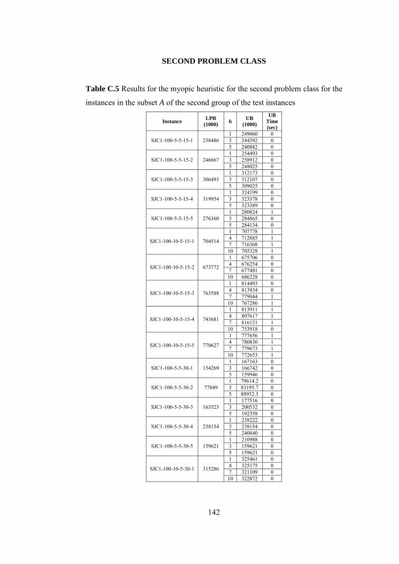
142

SECOND PROBLEM CLASS

Table C.5 Results for the myopic heuristic for the second problem class for the

instances in the subset A of the second group of the test instances

Instance LPR

(1000) h

UB

(1000)

UB

Time

(sec)

SJC1-100-5-5-15-1 238486 1 249060 0 3 244392 0 5 240882 0

SJC1-100-5-5-15-2 246667 1 254493 0 3 258912 0 5 248025 0

SJC1-100-5-5-15-3 306493 1 312173 0 3 312107 0 5 309025 0

SJC1-100-5-5-15-4 319954 1 324199 0 3 323378 0 5 323389 0

SJC1-100-5-5-15-5 276360 1 280824 1 3 284865 0 5 284134 0

SJC1-100-10-5-15-1 704514

1 707778 1 4 712885 1 7 716368 1

10 705328 1

SJC1-100-10-5-15-2 673772

1 675706 0 4 676254 0 7 677481 0

10 686228 0

SJC1-100-10-5-15-3 763588

1 814493 0 4 813934 0 7 779044 1

10 767286 1

SJC1-100-10-5-15-4 743681

1 813911 1 4 807617 1 7 816121 1

10 753918 0

SJC1-100-10-5-15-5 770627

1 777656 1 4 780830 1 7 779673 1

10 772653 1

SJC1-100-5-5-30-1 154269 1 167163 0 3 166742 0 5 159946 0

SJC1-100-5-5-30-2 77849 1 79614.2 0 3 83195.7 0 5 88932.3 0

SJC1-100-5-5-30-3 163523 1 177516 0 3 200532 0 5 192358 0

SJC1-100-5-5-30-4 238154 1 238222 0 3 238154 0 5 240840 0

SJC1-100-5-5-30-5 159621 1 210988 0 3 159621 0 5 159621 0

SJC1-100-10-5-30-1 315286

1 325461 0 4 325175 0 7 321109 0

10 322872 0

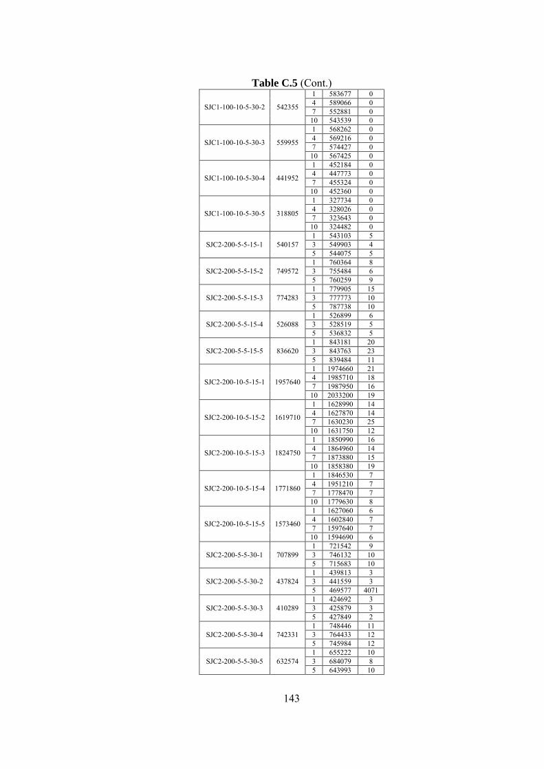
143

Table C.5 (Cont.)

SJC1-100-10-5-30-2 542355

1 583677 0 4 589066 0 7 552881 0

10 543539 0

SJC1-100-10-5-30-3 559955

1 568262 0 4 569216 0 7 574427 0

10 567425 0

SJC1-100-10-5-30-4 441952

1 452184 0 4 447773 0 7 455324 0

10 452360 0

SJC1-100-10-5-30-5 318805

1 327734 0 4 328026 0 7 323643 0

10 324482 0

SJC2-200-5-5-15-1 540157 1 543103 5 3 549903 4 5 544075 5

SJC2-200-5-5-15-2 749572 1 760364 8 3 755484 6 5 760259 9

SJC2-200-5-5-15-3 774283 1 779905 15 3 777773 10 5 787738 10

SJC2-200-5-5-15-4 526088 1 526899 6 3 528519 5 5 536832 5

SJC2-200-5-5-15-5 836620 1 843181 20 3 843763 23 5 839484 11

SJC2-200-10-5-15-1 1957640

1 1974660 21 4 1985710 18 7 1987950 16

10 2033200 19

SJC2-200-10-5-15-2 1619710

1 1628990 14 4 1627870 14 7 1630230 25

10 1631750 12

SJC2-200-10-5-15-3 1824750

1 1850990 16 4 1864960 14 7 1873880 15

10 1858380 19

SJC2-200-10-5-15-4 1771860

1 1846530 7 4 1951210 7 7 1778470 7

10 1779630 8

SJC2-200-10-5-15-5 1573460

1 1627060 6 4 1602840 7 7 1597640 7

10 1594690 6

SJC2-200-5-5-30-1 707899 1 721542 9 3 746132 10 5 715683 10

SJC2-200-5-5-30-2 437824 1 439813 3 3 441559 3 5 469577 4071

SJC2-200-5-5-30-3 410289 1 424692 3 3 425879 3 5 427849 2

SJC2-200-5-5-30-4 742331 1 748446 11 3 764433 12 5 745984 12

SJC2-200-5-5-30-5 632574 1 655222 10 3 684079 8 5 643993 10

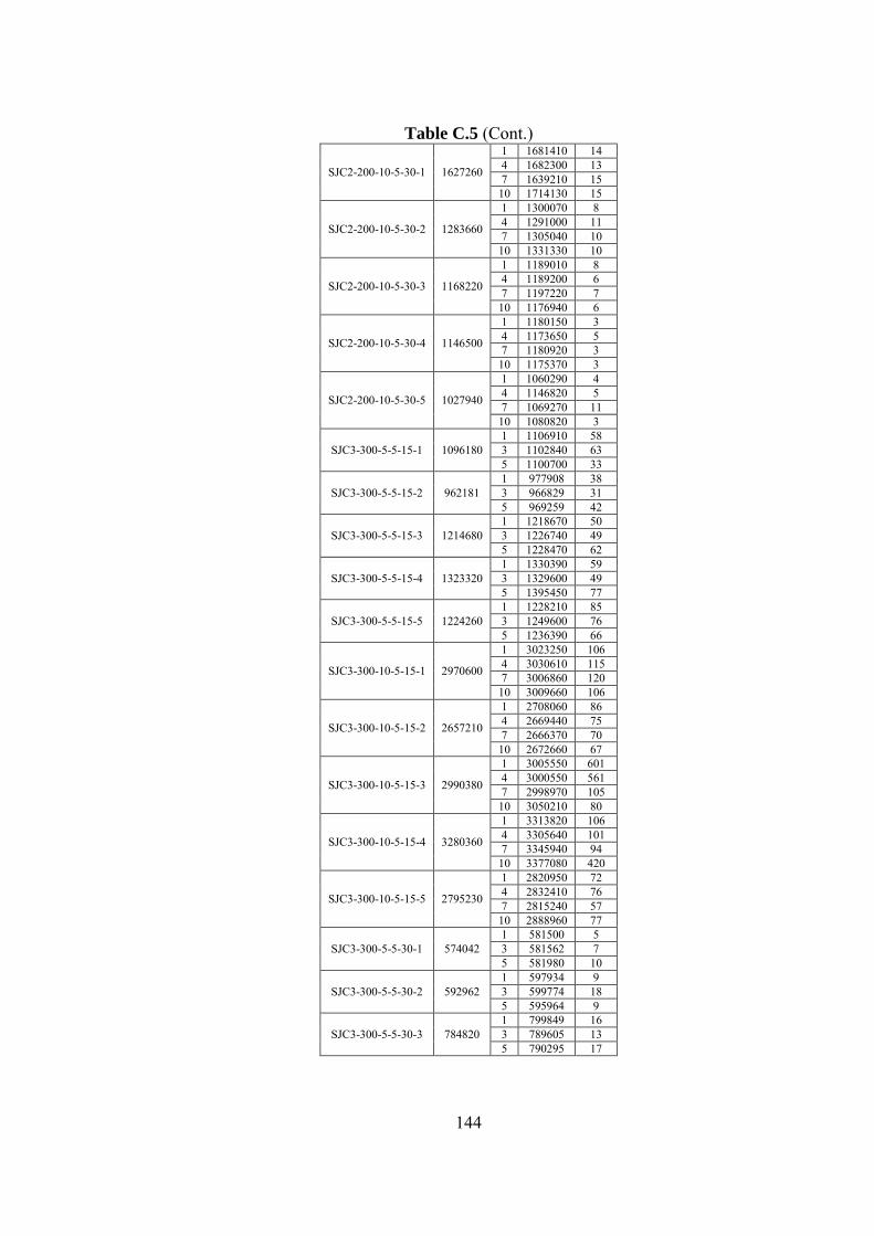
144

Table C.5 (Cont.)

SJC2-200-10-5-30-1 1627260

1 1681410 14 4 1682300 13 7 1639210 15

10 1714130 15

SJC2-200-10-5-30-2 1283660

1 1300070 8 4 1291000 11 7 1305040 10

10 1331330 10

SJC2-200-10-5-30-3 1168220

1 1189010 8 4 1189200 6 7 1197220 7

10 1176940 6

SJC2-200-10-5-30-4 1146500

1 1180150 3 4 1173650 5 7 1180920 3

10 1175370 3

SJC2-200-10-5-30-5 1027940

1 1060290 4 4 1146820 5 7 1069270 11

10 1080820 3

SJC3-300-5-5-15-1 1096180 1 1106910 58 3 1102840 63 5 1100700 33

SJC3-300-5-5-15-2 962181 1 977908 38 3 966829 31 5 969259 42

SJC3-300-5-5-15-3 1214680 1 1218670 50 3 1226740 49 5 1228470 62

SJC3-300-5-5-15-4 1323320 1 1330390 59 3 1329600 49 5 1395450 77

SJC3-300-5-5-15-5 1224260 1 1228210 85 3 1249600 76 5 1236390 66

SJC3-300-10-5-15-1 2970600

1 3023250 106 4 3030610 115 7 3006860 120

10 3009660 106

SJC3-300-10-5-15-2 2657210

1 2708060 86 4 2669440 75 7 2666370 70

10 2672660 67

SJC3-300-10-5-15-3 2990380

1 3005550 601 4 3000550 561 7 2998970 105

10 3050210 80

SJC3-300-10-5-15-4 3280360

1 3313820 106 4 3305640 101 7 3345940 94

10 3377080 420

SJC3-300-10-5-15-5 2795230

1 2820950 72 4 2832410 76 7 2815240 57

10 2888960 77

SJC3-300-5-5-30-1 574042 1 581500 5 3 581562 7 5 581980 10

SJC3-300-5-5-30-2 592962 1 597934 9 3 599774 18 5 595964 9

SJC3-300-5-5-30-3 784820 1 799849 16 3 789605 13 5 790295 17

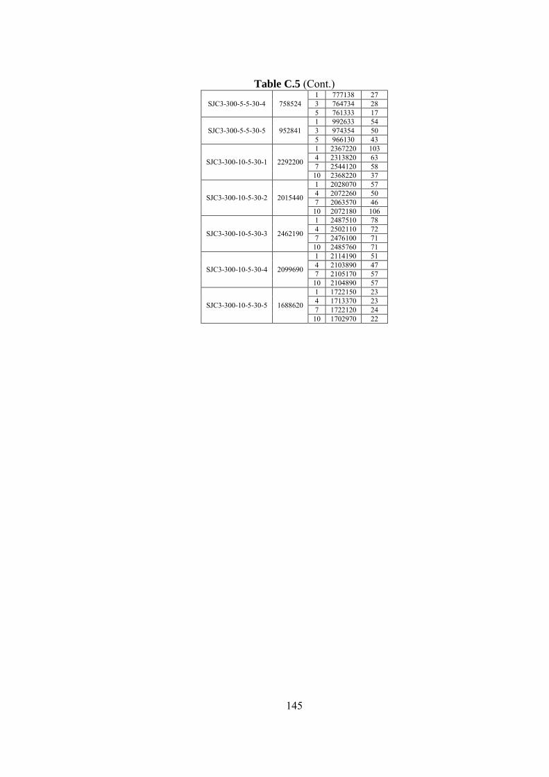
145

Table C.5 (Cont.)

SJC3-300-5-5-30-4 758524 1 777138 27 3 764734 28 5 761333 17

SJC3-300-5-5-30-5 952841 1 992633 54 3 974354 50 5 966130 43

SJC3-300-10-5-30-1 2292200

1 2367220 103 4 2313820 63 7 2544120 58

10 2368220 37

SJC3-300-10-5-30-2 2015440

1 2028070 57 4 2072260 50 7 2063570 46

10 2072180 106

SJC3-300-10-5-30-3 2462190

1 2487510 78 4 2502110 72 7 2476100 71

10 2485760 71

SJC3-300-10-5-30-4 2099690

1 2114190 51 4 2103890 47 7 2105170 57

10 2104890 57

SJC3-300-10-5-30-5 1688620

1 1722150 23 4 1713370 23 7 1722120 24

10 1702970 22

146

Table C.6 Results for the progressive heuristics for the second problem class

for the instances in the subset A of the second group of the test instances

Instance LPR

(1000) h

Progressive-1 Progressive-2

UB

(1000)

UB

Time

(sec)

UB

(1000)

UB

Time

(sec)

SJC1-100-5-5-15-1 238486 1 256061 0 257625 0 T* 248456 0 252511 0

SJC1-100-5-5-15-2 246667 1 261363 0 279087 0 T* 271713 0 273360 0

SJC1-100-5-5-15-3 306493 1 326257 0 331730 0 T* 322957 0 334958 0

SJC1-100-5-5-15-4 319954 1 341413 0 334226 0 T* 361217 0 366707 0

SJC1-100-5-5-15-5 276360 1 300361 0 290959 0 T* 303263 0 305978 0

SJC1-100-10-5-15-1 704514 1 744914 0 761553 0 T* 758701 0 750232 1

SJC1-100-10-5-15-2 673772 1 738309 0 741972 0 T* 801409 0 774831 0

SJC1-100-10-5-15-3 763588 1 818043 0 812174 0 T* 780896 0 782762 1

SJC1-100-10-5-15-4 743681 1 807516 0 805099 0 T* 780320 0 771543 1

SJC1-100-10-5-15-5 770627 1 820077 0 812245 0 T* 859165 0 859165 1

SJC1-100-5-5-30-1 154269 1 166110 0 165993 0 T* 274287 0 274298 0

SJC1-100-5-5-30-2 77849 1 111472 0 91647.2 0 T* 85970.4 0 88380.3 0

SJC1-100-5-5-30-3 16352 1 181795 0 176227 0 T* 181855 0 176118 0

SJC1-100-5-5-30-4 238154 1 310110 0 253647 0 T* 287069 0 287069 0

SJC1-100-5-5-30-5 159621 1 165224 0 173484 0 T* 230019 0 231525 0

SJC1-100-10-5-30-1 315286 1 476279 0 364222 0 T* 351189 0 356418 0

SJC1-100-10-5-30-2 542355 1 588894 0 587361 0 T* 713853 0 681699 0

SJC1-100-10-5-30-3 559955 1 614636 0 602661 0 T* 646395 0 589094 0

SJC1-100-10-5-30-4 441952 1 491822 0 499196 0 T* 493478 0 484840 1

SJC1-100-10-5-30-5 318805 1 338038 0 349475 0 T* 388990 0 358428 0

SJC2-200-5-5-15-1 540157 1 566968 1 564539 2 T* 698165 2 699561 6

SJC2-200-5-5-15-2 749572 1 789367 5 791668 6 T* 805866 10 805109 11

SJC2-200-5-5-15-3 774283 1 804348 4 803903 6 T* 846824 8 837896 15

SJC2-200-5-5-15-4 526088 1 576338 2 584099 5 T* 570445 5 578795 9

SJC2-200-5-5-15-5 836620 1 876962 6 862601 10 T* 922491 12 928521 20

SJC2-200-10-5-15-1 1957640 1 2078330 7 2088890 10 T* 2079120 13 2118420 29

SJC2-200-10-5-15-2 1619710 1 1717970 4 1716510 5 T* 1720350 10 1728540 14

SJC2-200-10-5-15-3 1824750 1 1948230 6 1948230 7 T* 1952580 15 1923920 17

SJC2-200-10-5-15-4 1771860 1 1856320 5 1843000 7 T* 1883900 15 1864420 20

SJC2-200-10-5-15-5 1573460 1 1681290 1 1634400 4 T* 1661050 5 1663260 9

147

Table C.6 (Cont.) SJC2-200-5-5-30-1 707899 1 729886 4 730177 4

T* 865128 10 813023 10

SJC2-200-5-5-30-2 437824 1 471115 2 466105 2 T* 512766 3 493982 4

SJC2-200-5-5-30-3 410289 1 451521 2 446130 4 T* 438981 2 426839 6

SJC2-200-5-5-30-4 742331 1 776174 5 783878 7 T* 832786 12 835549 14

SJC2-200-5-5-30-5 632574 1 669047 5 656677 8 T* 710315 12 710315 10

SJC2-200-10-5-30-1 1627260 1 1740210 7 1743240 9 T* 1860490 21 1862190 18

SJC2-200-10-5-30-2 1283660 1 1350940 3 1401010 7 T* 1399570 14 1375210 17

SJC2-200-10-5-30-3 1168220 1 1267400 3 1299980 5 T* 1277790 6 1240470 14

SJC2-200-10-5-30-4 1146500 1 1209380 4 1208150 4 T* 1555080 4 1555810 5

SJC2-200-10-5-30-5 1027940 1 1128640 1 1102620 4 T* 1137810 4 1131500 7

SJC3-300-5-5-15-1 1096180 1 1132810 23 1151370 25 T* 1148910 34 1148910 51

SJC3-300-5-5-15-2 962181 1 1037030 11 1010560 30 T* 1001500 30 1018580 69

SJC3-300-5-5-15-3 1214680 1 1236930 31 1236930 32 T* 1243690 46 1243690 69

SJC3-300-5-5-15-4 1323320 1 1358090 37 1369190 36 T* 1397150 37 1399370 47

SJC3-300-5-5-15-5 1224260 1 1263330 44 1257180 45 T* 1315840 45 1323490 59

SJC3-300-10-5-15-1 2970600 1 3102980 36 3116530 45 T* 3526200 54 3456630 88

SJC3-300-10-5-15-2 2657210 1 2810590 35 2789170 49 T* 2790590 54 2789930 97

SJC3-300-10-5-15-3 2990380 1 3096470 40 3093040 38 T* 3103080 75 3119050 82

SJC3-300-10-5-15-4 3280360 1 3437250 45 3423730 55 T* 3459320 77 3465090 102

SJC3-300-10-5-15-5 2795230 1 2903540 20 2877900 46 T* 2912610 45 2933510 77

SJC3-300-5-5-30-1 574042 1 596280 3 619429 4 T* 605070 5 612988 11

SJC3-300-5-5-30-2 592962 1 664316 3 635833 7 T* 643792 10 647095 20

SJC3-300-5-5-30-3 784820 1 814533 7 812308 22 T* 852779 17 870398 29

SJC3-300-5-5-30-4 758524 1 805157 17 807294 20 T* 799702 12 800837 23

SJC3-300-5-5-30-5 952841 1 985224 36 982458 36 T* 1049370 43 1051310 35

SJC3-300-10-5-30-1 2292200 1 2433430 33 2424680 43 T* 2499250 45 2446540 74

SJC3-300-10-5-30-2 2015440 1 2126600 26 2107850 36 T* 2360700 45 2352080 45

SJC3-300-10-5-30-3 2462190 1 2558620 32 2548960 53 T* 2587750 57 2569360 75

SJC3-300-10-5-30-4 2099690 1 2194440 11 2201510 19 T* 2356900 23 2209960 48

SJC3-300-10-5-30-5 1688620 1 1784690 9 1813400 13 T* 1914200 19 1846480 30

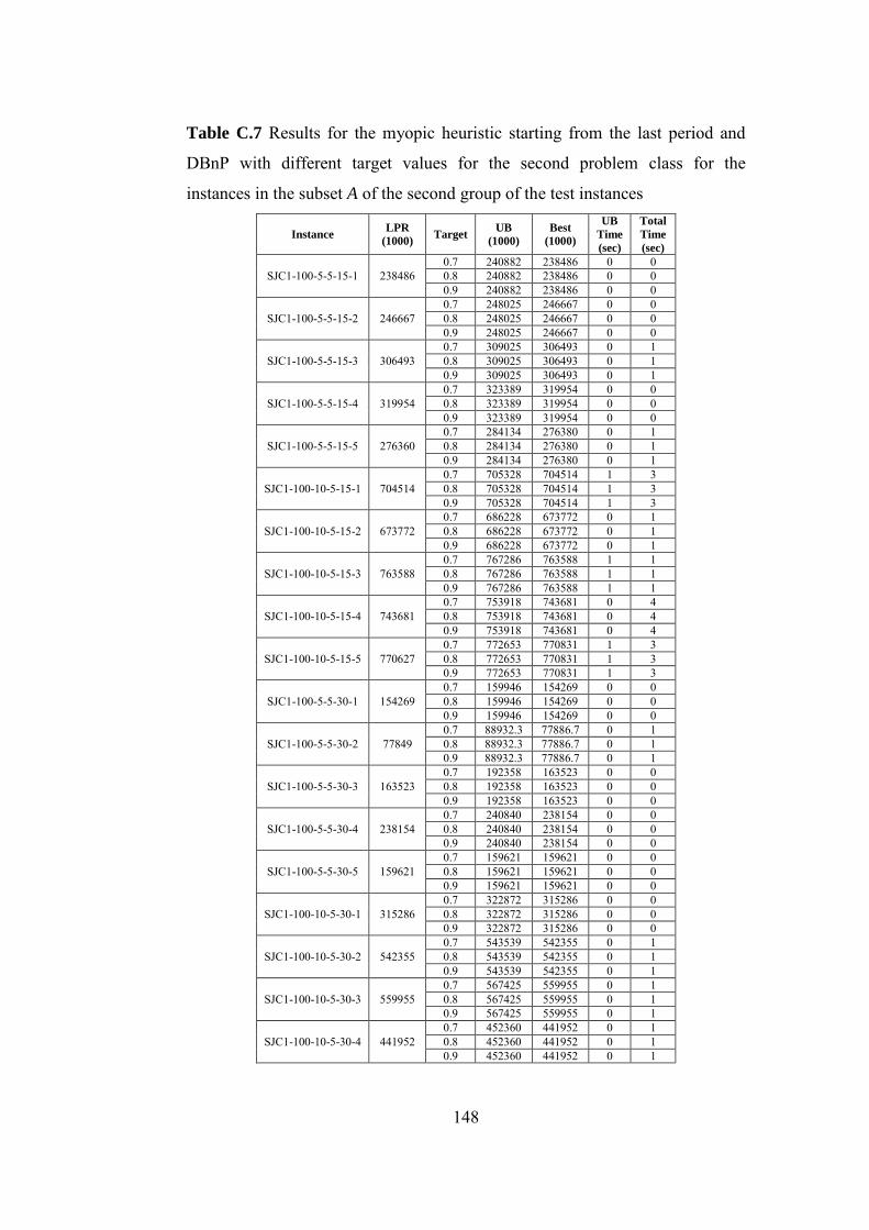
148

Table C.7 Results for the myopic heuristic starting from the last period and

DBnP with different target values for the second problem class for the

instances in the subset A of the second group of the test instances

Instance LPR

(1000) Target

UB

(1000)

Best

(1000)

UB

Time

(sec)

Total

Time

(sec)

SJC1-100-5-5-15-1 238486 0.7 240882 238486 0 0 0.8 240882 238486 0 0 0.9 240882 238486 0 0

SJC1-100-5-5-15-2 246667 0.7 248025 246667 0 0 0.8 248025 246667 0 0 0.9 248025 246667 0 0

SJC1-100-5-5-15-3 306493 0.7 309025 306493 0 1 0.8 309025 306493 0 1 0.9 309025 306493 0 1

SJC1-100-5-5-15-4 319954 0.7 323389 319954 0 0 0.8 323389 319954 0 0 0.9 323389 319954 0 0

SJC1-100-5-5-15-5 276360 0.7 284134 276380 0 1 0.8 284134 276380 0 1 0.9 284134 276380 0 1

SJC1-100-10-5-15-1 704514 0.7 705328 704514 1 3 0.8 705328 704514 1 3 0.9 705328 704514 1 3

SJC1-100-10-5-15-2 673772 0.7 686228 673772 0 1 0.8 686228 673772 0 1 0.9 686228 673772 0 1

SJC1-100-10-5-15-3 763588 0.7 767286 763588 1 1 0.8 767286 763588 1 1 0.9 767286 763588 1 1

SJC1-100-10-5-15-4 743681 0.7 753918 743681 0 4 0.8 753918 743681 0 4 0.9 753918 743681 0 4

SJC1-100-10-5-15-5 770627 0.7 772653 770831 1 3 0.8 772653 770831 1 3 0.9 772653 770831 1 3

SJC1-100-5-5-30-1 154269 0.7 159946 154269 0 0 0.8 159946 154269 0 0 0.9 159946 154269 0 0

SJC1-100-5-5-30-2 77849 0.7 88932.3 77886.7 0 1 0.8 88932.3 77886.7 0 1 0.9 88932.3 77886.7 0 1

SJC1-100-5-5-30-3 163523 0.7 192358 163523 0 0 0.8 192358 163523 0 0 0.9 192358 163523 0 0

SJC1-100-5-5-30-4 238154 0.7 240840 238154 0 0 0.8 240840 238154 0 0 0.9 240840 238154 0 0

SJC1-100-5-5-30-5 159621 0.7 159621 159621 0 0 0.8 159621 159621 0 0 0.9 159621 159621 0 0

SJC1-100-10-5-30-1 315286 0.7 322872 315286 0 0 0.8 322872 315286 0 0 0.9 322872 315286 0 0

SJC1-100-10-5-30-2 542355 0.7 543539 542355 0 1 0.8 543539 542355 0 1 0.9 543539 542355 0 1

SJC1-100-10-5-30-3 559955 0.7 567425 559955 0 1 0.8 567425 559955 0 1 0.9 567425 559955 0 1

SJC1-100-10-5-30-4 441952 0.7 452360 441952 0 1 0.8 452360 441952 0 1 0.9 452360 441952 0 1

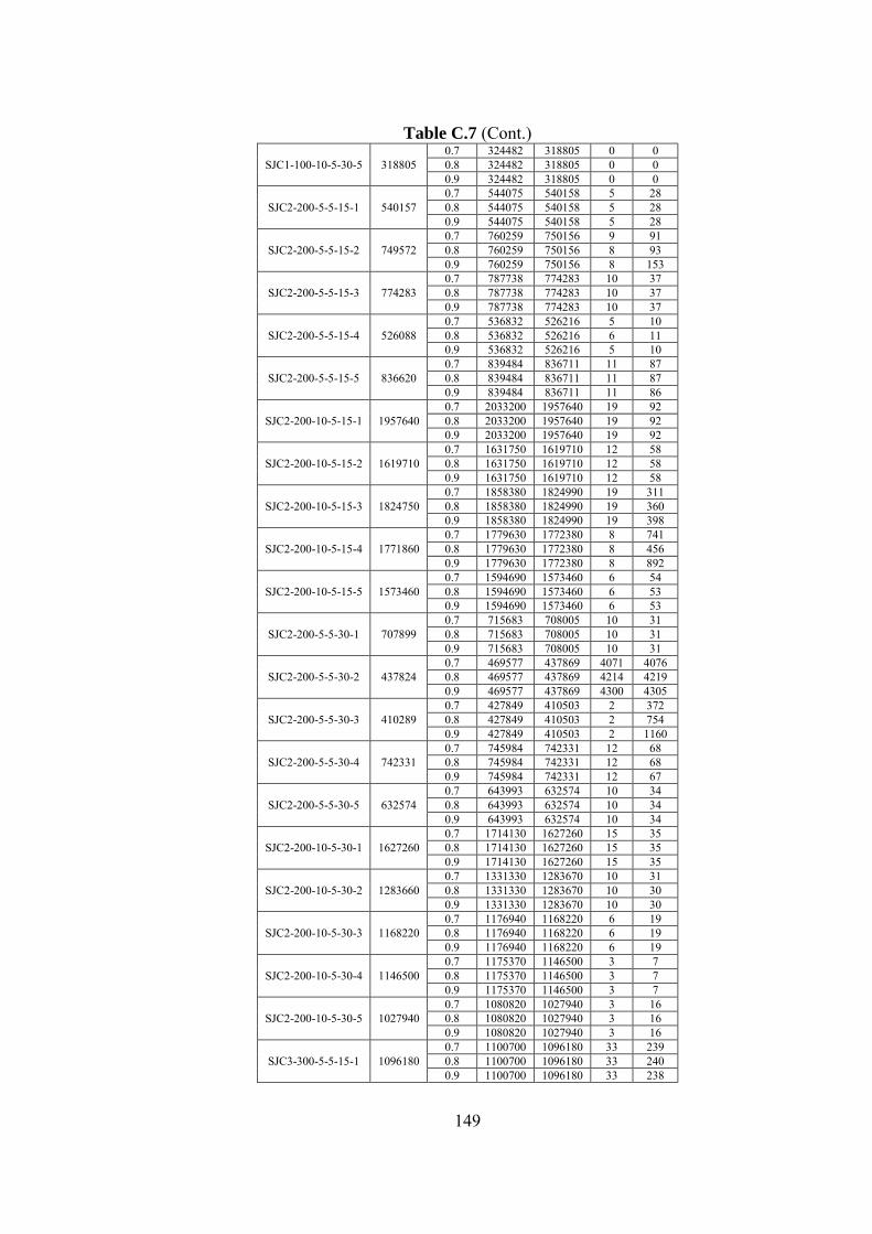
149

Table C.7 (Cont.)

SJC1-100-10-5-30-5 318805 0.7 324482 318805 0 0 0.8 324482 318805 0 0 0.9 324482 318805 0 0

SJC2-200-5-5-15-1 540157 0.7 544075 540158 5 28 0.8 544075 540158 5 28 0.9 544075 540158 5 28

SJC2-200-5-5-15-2 749572 0.7 760259 750156 9 91 0.8 760259 750156 8 93 0.9 760259 750156 8 153

SJC2-200-5-5-15-3 774283 0.7 787738 774283 10 37 0.8 787738 774283 10 37 0.9 787738 774283 10 37

SJC2-200-5-5-15-4 526088 0.7 536832 526216 5 10 0.8 536832 526216 6 11 0.9 536832 526216 5 10

SJC2-200-5-5-15-5 836620 0.7 839484 836711 11 87 0.8 839484 836711 11 87 0.9 839484 836711 11 86

SJC2-200-10-5-15-1 1957640 0.7 2033200 1957640 19 92 0.8 2033200 1957640 19 92 0.9 2033200 1957640 19 92

SJC2-200-10-5-15-2 1619710 0.7 1631750 1619710 12 58 0.8 1631750 1619710 12 58 0.9 1631750 1619710 12 58

SJC2-200-10-5-15-3 1824750 0.7 1858380 1824990 19 311 0.8 1858380 1824990 19 360 0.9 1858380 1824990 19 398

SJC2-200-10-5-15-4 1771860 0.7 1779630 1772380 8 741 0.8 1779630 1772380 8 456 0.9 1779630 1772380 8 892

SJC2-200-10-5-15-5 1573460 0.7 1594690 1573460 6 54 0.8 1594690 1573460 6 53 0.9 1594690 1573460 6 53

SJC2-200-5-5-30-1 707899 0.7 715683 708005 10 31 0.8 715683 708005 10 31 0.9 715683 708005 10 31

SJC2-200-5-5-30-2 437824 0.7 469577 437869 4071 4076 0.8 469577 437869 4214 4219 0.9 469577 437869 4300 4305

SJC2-200-5-5-30-3 410289 0.7 427849 410503 2 372 0.8 427849 410503 2 754 0.9 427849 410503 2 1160

SJC2-200-5-5-30-4 742331 0.7 745984 742331 12 68 0.8 745984 742331 12 68 0.9 745984 742331 12 67

SJC2-200-5-5-30-5 632574 0.7 643993 632574 10 34 0.8 643993 632574 10 34 0.9 643993 632574 10 34

SJC2-200-10-5-30-1 1627260 0.7 1714130 1627260 15 35 0.8 1714130 1627260 15 35 0.9 1714130 1627260 15 35

SJC2-200-10-5-30-2 1283660 0.7 1331330 1283670 10 31 0.8 1331330 1283670 10 30 0.9 1331330 1283670 10 30

SJC2-200-10-5-30-3 1168220 0.7 1176940 1168220 6 19 0.8 1176940 1168220 6 19 0.9 1176940 1168220 6 19

SJC2-200-10-5-30-4 1146500 0.7 1175370 1146500 3 7 0.8 1175370 1146500 3 7 0.9 1175370 1146500 3 7

SJC2-200-10-5-30-5 1027940 0.7 1080820 1027940 3 16 0.8 1080820 1027940 3 16 0.9 1080820 1027940 3 16

SJC3-300-5-5-15-1 1096180 0.7 1100700 1096180 33 239 0.8 1100700 1096180 33 240 0.9 1100700 1096180 33 238

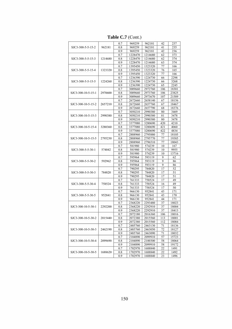
150

Table C.7 (Cont.)

SJC3-300-5-5-15-2 962181 0.7 969259 962181 42 237 0.8 969259 962181 41 235 0.9 969259 962181 42 236

SJC3-300-5-5-15-3 1214680 0.7 1228470 1214680 62 373 0.8 1228470 1214680 62 374 0.9 1228470 1214680 63 374

SJC3-300-5-5-15-4 1323320 0.7 1395450 1323320 77 166 0.8 1395450 1323320 76 165 0.9 1395450 1323320 77 166

SJC3-300-5-5-15-5 1224260 0.7 1236390 1224730 66 2298 0.8 1236390 1224730 66 3268 0.9 1236390 1224730 65 2245

SJC3-300-10-5-15-1 2970600 0.7 3009660 2972760 106 18301 0.8 3009660 2973760 106 23825 0.9 3009660 2973670 107 21589

SJC3-300-10-5-15-2 2657210 0.7 2672660 2658140 67 18156 0.8 2672660 2657760 67 18467 0.9 2672660 2657790 68 18376

SJC3-300-10-5-15-3 2990380 0.7 3050210 2990380 80 3469 0.8 3050210 2990380 81 3478 0.9 3050210 2990380 80 3478

SJC3-300-10-5-15-4 3280360 0.7 3377080 3280690 420 4210 0.8 3377080 3280690 421 4060 0.9 3377080 3280690 422 4834

SJC3-300-10-5-15-5 2795230 0.7 2888960 2795880 77 18105 0.8 2888960 2795770 77 19385 0.9 2888960 2796510 77 18043

SJC3-300-5-5-30-1 574042 0.7 581980 574239 10 167 0.8 581980 574239 10 9955 0.9 581980 574239 10 13716

SJC3-300-5-5-30-2 592962 0.7 595964 593119 9 62 0.8 595964 593119 9 86 0.9 595964 593119 9 86

SJC3-300-5-5-30-3 784820 0.7 790295 784820 17 52 0.8 790295 784820 17 51 0.9 790295 784820 17 51

SJC3-300-5-5-30-4 758524 0.7 761333 758524 17 49 0.8 761333 758524 16 49 0.9 761333 758524 17 50

SJC3-300-5-5-30-5 952841 0.7 966130 952841 43 171 0.8 966130 952841 43 170 0.9 966130 952841 44 171

SJC3-300-10-5-30-1 2292200 0.7 2368220 2293480 37 18023 0.8 2368220 2292910 37 18004 0.9 2368220 2292910 37 18413

SJC3-300-10-5-30-2 2015440 0.7 2072180 2016360 106 18016 0.8 2072380 2015560 113 18001 0.9 2072380 2015560 112 18084

SJC3-300-10-5-30-3 2462190 0.7 2485760 2463130 71 18136 0.8 2485760 2463050 72 18127 0.9 2485760 2463090 71 18032

SJC3-300-10-5-30-4 2099690 0.7 2104890 2099910 57 15723 0.8 2104890 2100300 58 18064 0.9 2104890 2099910 58 19172

SJC3-300-10-5-30-5 1688620 0.7 1702970 1688840 22 1491 0.8 1702970 1688840 22 1492 0.9 1702970 1688840 23 1496

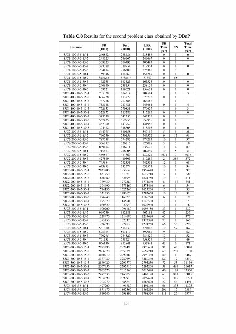
151

Table C.8 Results for the second problem class obtained by DBnP

Instance UB

(1000)

Best

(1000)

LPR

(1000)

UB

Time

(sec)

NN

Total

Time

(sec)

SJC1-100-5-5-15-1 240882 238486 238486 0 1 0 SJC1-100-5-5-15-2 248025 246667 246667 0 1 0 SJC1-100-5-5-15-3 309025 306493 306493 0 1 1 SJC1-100-5-5-15-4 323389 319954 319954 0 1 0 SJC1-100-5-5-15-5 284134 276380 276360 0 9 1 SJC1-100-5-5-30-1 159946 154269 154269 0 1 0 SJC1-100-5-5-30-2 88932.3 77886.7 77849 0 55 1 SJC1-100-5-5-30-3 192358 163523 163523 0 1 0 SJC1-100-5-5-30-4 240840 238154 238154 0 1 0 SJC1-100-5-5-30-5 159621 159621 159621 0 1 0 SJC1-100-10-5-15-1 705328 704514 704514 1 1 3 SJC1-100-10-5-15-2 686228 673772 673772 0 1 1 SJC1-100-10-5-15-3 767286 763588 763588 1 1 1 SJC1-100-10-5-15-4 753918 743681 743681 0 1 4 SJC1-100-10-5-15-5 772653 770831 770627 1 9 3 SJC1-100-10-5-30-1 322872 315286 315286 0 1 0 SJC1-100-10-5-30-2 543539 542355 542355 0 1 1 SJC1-100-10-5-30-3 567425 559955 559955 0 1 1 SJC1-100-10-5-30-4 452360 441952 441952 0 1 1 SJC1-100-10-5-30-5 324482 318805 318805 0 1 0 SJC2-200-5-5-15-1 544075 540158 540157 5 5 28 SJC2-200-5-5-15-2 760259 750156 749572 9 15 91 SJC2-200-5-5-15-3 787738 774283 774283 10 1 37 SJC2-200-5-5-15-4 536832 526216 526088 5 5 10 SJC2-200-5-5-15-5 839484 836711 836620 11 4 87 SJC2-200-5-5-30-1 715683 708005 707899 10 5 31 SJC2-200-5-5-30-2 469577 437869 437824 4071 3 4076 SJC2-200-5-5-30-3 427849 410503 410289 2 389 372 SJC2-200-5-5-30-4 745984 742331 742331 12 3 68 SJC2-200-5-5-30-5 643993 632574 632574 10 1 34 SJC2-200-10-5-15-1 2033200 1957640 1957640 19 1 92 SJC2-200-10-5-15-2 1631750 1619710 1619710 12 1 58 SJC2-200-10-5-15-3 1858380 1824990 1824750 19 13 311 SJC2-200-10-5-15-4 1779630 1772380 1771860 8 117 741 SJC2-200-10-5-15-5 1594690 1573460 1573460 6 1 54 SJC2-200-10-5-30-1 1714130 1627260 1627260 15 1 35 SJC2-200-10-5-30-2 1331330 1283670 1283660 10 13 31 SJC2-200-10-5-30-3 1176940 1168220 1168220 6 1 19 SJC2-200-10-5-30-4 1175370 1146500 1146500 3 1 7 SJC2-200-10-5-30-5 1080820 1027940 1027940 3 1 16 SJC3-300-5-5-15-1 1100700 1096180 1096180 33 1 239 SJC3-300-5-5-15-2 969259 962181 962181 42 5 237 SJC3-300-5-5-15-3 1228470 1214680 1214680 62 1 373 SJC3-300-5-5-15-4 1395450 1323320 1323320 77 1 166 SJC3-300-5-5-15-5 1236390 1224730 1224260 66 55 2298 SJC3-300-5-5-30-1 581980 574239 574042 10 57 167 SJC3-300-5-5-30-2 595964 593119 592962 9 10 62 SJC3-300-5-5-30-3 790295 784820 784820 17 1 52 SJC3-300-5-5-30-4 761333 758524 758524 17 1 49 SJC3-300-5-5-30-5 966130 952841 952841 43 6 171 SJC3-300-10-5-15-1 2993790 2972490 2970600 91 43 36020 SJC3-300-10-5-15-2 2666370 2657790 2657210 69 298 36180 SJC3-300-10-5-15-3 3050210 2990380 2990380 80 1 3469 SJC3-300-10-5-15-4 3377080 3280690 3280360 420 17 4210 SJC3-300-10-5-15-5 2869020 2795770 2795230 72 53 31156 SJC3-300-10-5-30-1 2507950 2292910 2292200 58 466 36017 SJC3-300-10-5-30-2 2063570 2015560 2015440 46 169 12560 SJC3-300-10-5-30-3 2477630 2463050 2462190 63 803 36015 SJC3-300-10-5-30-4 2104890 2099910 2099690 57 305 15723 SJC3-300-10-5-30-5 1702970 1688840 1688620 22 54 1491 SJC4-402-5-5-15-1 1497700 1491880 1491360 66 335 11375 SJC4-402-5-5-15-2 1871670 1862560 1862250 296 17 7389 SJC4-402-5-5-15-3 1810240 1798890 1798350 111 27 7979

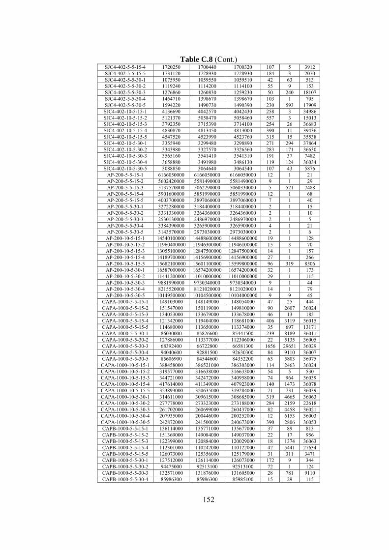
152

Table C.8 (Cont.) SJC4-402-5-5-15-4 1720250 1700440 1700320 107 5 3912 SJC4-402-5-5-15-5 1731120 1728930 1728930 184 3 2070 SJC4-402-5-5-30-1 1075950 1059550 1059510 42 63 513 SJC4-402-5-5-30-2 1119240 1114200 1114100 55 9 153 SJC4-402-5-5-30-3 1276860 1260830 1259230 50 240 18107 SJC4-402-5-5-30-4 1464710 1398670 1398670 103 1 705 SJC4-402-5-5-30-5 1594220 1490730 1490390 230 593 17909 SJC4-402-10-5-15-1 4136690 4042570 4042430 258 3 34986 SJC4-402-10-5-15-2 5121370 5058470 5058460 557 3 15013 SJC4-402-10-5-15-3 3792350 3715390 3714100 254 26 36683 SJC4-402-10-5-15-4 4830870 4813450 4813000 390 11 39436 SJC4-402-10-5-15-5 4547520 4523990 4523760 315 15 35538 SJC4-402-10-5-30-1 3355940 3299480 3298890 271 294 37864 SJC4-402-10-5-30-2 3343980 3327570 3326560 283 171 36630 SJC4-402-10-5-30-3 3565160 3541410 3541310 191 37 7482 SJC4-402-10-5-30-4 3658880 3491980 3486130 119 124 36034 SJC4-402-10-5-30-5 3088850 3064640 3064540 107 43 5876

AP-200-5-5-15-1 6166050000 6166050000 6166050000 12 1 21 AP-200-5-5-15-2 5602420000 5581490000 5581490000 9 1 29 AP-200-5-5-15-3 5137570000 5062290000 5060330000 5 521 7488 AP-200-5-5-15-4 5901600000 5851990000 5851990000 12 1 68 AP-200-5-5-15-5 4003700000 3897060000 3897060000 7 1 40 AP-200-5-5-30-1 3272280000 3184400000 3184400000 2 1 15 AP-200-5-5-30-2 3331330000 3264360000 3264360000 2 1 10 AP-200-5-5-30-3 2530130000 2486970000 2486970000 2 1 5 AP-200-5-5-30-4 3384390000 3265900000 3265900000 4 1 21 AP-200-5-5-30-5 3143570000 2973030000 2973030000 2 1 6 AP-200-10-5-15-1 14540100000 14488600000 14488600000 19 1 128 AP-200-10-5-15-2 11960400000 11946300000 11946100000 15 3 70 AP-200-10-5-15-3 13055100000 12847500000 12847500000 14 1 157 AP-200-10-5-15-4 14189700000 14156900000 14156900000 27 1 266 AP-200-10-5-15-5 15682100000 15601100000 15599800000 96 319 8506 AP-200-10-5-30-1 16587000000 16574200000 16574200000 32 1 173 AP-200-10-5-30-2 11441200000 11010000000 11010000000 29 1 115 AP-200-10-5-30-3 9881990000 9730340000 9730340000 9 1 44 AP-200-10-5-30-4 8215520000 8121020000 8121020000 14 1 79 AP-200-10-5-30-5 10149500000 10104500000 10104000000 9 9 45

CAPA-1000-5-5-15-1 149103000 148149000 148054000 47 25 444 CAPA-1000-5-5-15-2 151547000 150119000 149810000 90 2607 36024 CAPA-1000-5-5-15-3 134053000 133679000 133678000 46 13 185 CAPA-1000-5-5-15-4 121342000 119404000 118681000 406 3119 36015 CAPA-1000-5-5-15-5 114680000 113650000 113374000 35 697 13171 CAPA-1000-5-5-30-1 86030000 85826600 85441500 239 8189 36011 CAPA-1000-5-5-30-2 127886000 113377000 112306000 22 5135 36005 CAPA-1000-5-5-30-3 68392400 66722800 66581300 1656 29651 36029 CAPA-1000-5-5-30-4 94040600 92881500 92630300 84 9110 36007 CAPA-1000-5-5-30-5 85606900 84544600 84352200 63 5803 36075 CAPA-1000-10-5-15-1 388458000 386521000 386303000 114 2463 36024 CAPA-1000-10-5-15-2 319577000 316638000 316633000 54 5 530 CAPA-1000-10-5-15-3 344721000 342472000 340958000 74 964 36039 CAPA-1000-10-5-15-4 417614000 411349000 407923000 140 1473 36078 CAPA-1000-10-5-15-5 323893000 320635000 319284000 71 731 36039 CAPA-1000-10-5-30-1 314611000 309615000 308685000 319 4665 36063 CAPA-1000-10-5-30-2 277778000 273323000 273188000 284 2159 22618 CAPA-1000-10-5-30-3 261702000 260699000 260437000 82 4458 36021 CAPA-1000-10-5-30-4 207935000 200446000 200252000 12 6153 36003 CAPA-1000-10-5-30-5 242872000 241500000 240673000 390 2806 36053 CAPB-1000-5-5-15-1 136114000 135771000 135677000 37 89 813 CAPB-1000-5-5-15-2 151369000 149084000 149037000 22 17 956 CAPB-1000-5-5-15-3 122399000 120884000 120029000 18 1374 36063 CAPB-1000-5-5-15-4 112301000 110242000 110122000 42 5441 27634 CAPB-1000-5-5-15-5 126073000 125356000 125179000 31 311 3471 CAPB-1000-5-5-30-1 127512000 126114000 126073000 172 9 344 CAPB-1000-5-5-30-2 94475000 92513100 92513100 72 1 124 CAPB-1000-5-5-30-3 132571000 131876000 131605000 28 781 9110 CAPB-1000-5-5-30-4 85986300 85986300 85985100 15 29 115

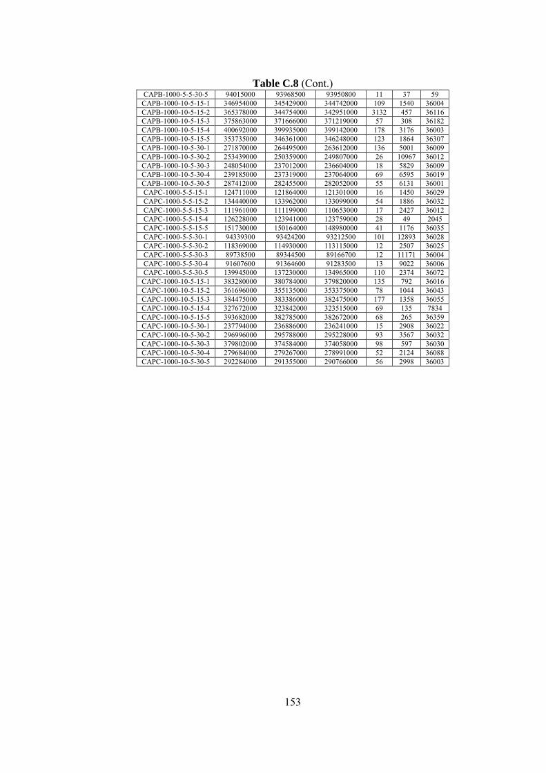
153

Table C.8 (Cont.) CAPB-1000-5-5-30-5 94015000 93968500 93950800 11 37 59

CAPB-1000-10-5-15-1 346954000 345429000 344742000 109 1540 36004 CAPB-1000-10-5-15-2 365378000 344754000 342951000 3132 457 36116 CAPB-1000-10-5-15-3 375863000 371666000 371219000 57 308 36182 CAPB-1000-10-5-15-4 400692000 399935000 399142000 178 3176 36003 CAPB-1000-10-5-15-5 353735000 346361000 346248000 123 1864 36307 CAPB-1000-10-5-30-1 271870000 264495000 263612000 136 5001 36009 CAPB-1000-10-5-30-2 253439000 250359000 249807000 26 10967 36012 CAPB-1000-10-5-30-3 248054000 237012000 236604000 18 5829 36009 CAPB-1000-10-5-30-4 239185000 237319000 237064000 69 6595 36019 CAPB-1000-10-5-30-5 287412000 282455000 282052000 55 6131 36001 CAPC-1000-5-5-15-1 124711000 121864000 121301000 16 1450 36029 CAPC-1000-5-5-15-2 134440000 133962000 133099000 54 1886 36032 CAPC-1000-5-5-15-3 111961000 111199000 110653000 17 2427 36012 CAPC-1000-5-5-15-4 126228000 123941000 123759000 28 49 2045 CAPC-1000-5-5-15-5 151730000 150164000 148980000 41 1176 36035 CAPC-1000-5-5-30-1 94339300 93424200 93212500 101 12893 36028 CAPC-1000-5-5-30-2 118369000 114930000 113115000 12 2507 36025 CAPC-1000-5-5-30-3 89738500 89344500 89166700 12 11171 36004 CAPC-1000-5-5-30-4 91607600 91364600 91283500 13 9022 36006 CAPC-1000-5-5-30-5 139945000 137230000 134965000 110 2374 36072

CAPC-1000-10-5-15-1 383280000 380784000 379820000 135 792 36016 CAPC-1000-10-5-15-2 361696000 355135000 353375000 78 1044 36043 CAPC-1000-10-5-15-3 384475000 383386000 382475000 177 1358 36055 CAPC-1000-10-5-15-4 327672000 323842000 323515000 69 135 7834 CAPC-1000-10-5-15-5 393682000 382785000 382672000 68 265 36359 CAPC-1000-10-5-30-1 237794000 236886000 236241000 15 2908 36022 CAPC-1000-10-5-30-2 296996000 295788000 295228000 93 3567 36032 CAPC-1000-10-5-30-3 379802000 374584000 374058000 98 597 36030 CAPC-1000-10-5-30-4 279684000 279267000 278991000 52 2124 36088 CAPC-1000-10-5-30-5 292284000 291355000 290766000 56 2998 36003

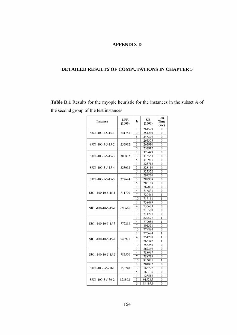
154

APPENDIX D

DETAILED RESULTS OF COMPUTATIONS IN CHAPTER 5

Table D.1 Results for the myopic heuristic for the instances in the subset A of

the second group of the test instances

Instance LPR

(1000) h

UB

(1000)

UB

Time

(sec)

SJC1-100-5-5-15-1 241785 1 261529 0 3 251240 0 5 248399 0

SJC1-100-5-5-15-2 252912 1 265375 0 3 262910 0 5 252912 0

SJC1-100-5-5-15-3 308872 1 329449 0 3 313553 0 5 310905 0

SJC1-100-5-5-15-4 323052 1 325713 0 3 328119 0 5 325322 0

SJC1-100-5-5-15-5 277694 1 297220 0 3 282988 0 5 285188 0

SJC1-100-10-5-15-1 711770

1 769098 0 4 716831 0 7 720468 1

10 717191 1

SJC1-100-10-5-15-2 690616

1 738499 0 4 736683 0 7 710580 0

10 711207 0

SJC1-100-10-5-15-3 772218

1 822527 1 4 779086 1 7 801351 0

10 779884 0

SJC1-100-10-5-15-4 748921

1 776694 1 4 754280 1 7 763342 1

10 753258 0

SJC1-100-10-5-15-5 785570

1 862369 0 4 788967 0 7 788739 0

10 815001 1

SJC1-100-5-5-30-1 158240 1 201802 0 3 163722 0 5 160136 0

SJC1-100-5-5-30-2 82389.1 1 128512 0 3 91523.3 0 5 84189.9 0

155

Table D.1 (Cont)

SJC1-100-5-5-30-3 161836 1 162166 0 3 162394 0 5 162394 0

SJC1-100-5-5-30-4 245473 1 281058 0 3 251802 0 5 245975 0

SJC1-100-5-5-30-5 159621 1 168221 0 3 159621 0 5 159621 0

SJC1-100-10-5-30-1 320506

1 333630 0 4 322592 0 7 322615 0

10 325766 0

SJC1-100-10-5-30-2 556427

1 623972 0 4 598596 0 7 563929 0

10 568519 0

SJC1-100-10-5-30-3 567070

1 612301 0 4 572353 0 7 574916 0

10 573818 0

SJC1-100-10-5-30-4 447455

1 462597 0 4 458389 0 7 453029 0

10 451264 0

SJC1-100-10-5-30-5 321096

1 341964 0 4 324943 0 7 332574 0

10 326081 0

SJC2-200-5-5-15-1 553710 1 666760 2 3 575129 1 5 556608 2

SJC2-200-5-5-15-2 755008 1 762608 3 3 759094 3 5 757877 3

SJC2-200-5-5-15-3 789996 1 820417 5 3 796335 4 5 796335 5

SJC2-200-5-5-15-4 539626 1 577850 2 3 551907 2 5 543624 2

SJC2-200-5-5-15-5 853995 1 875745 5 3 890656 7 5 874330 6

SJC2-200-10-5-15-1 1972970

1 2058280 9 4 2034810 9 7 1991440 10

10 1984900 9

SJC2-200-10-5-15-2 1649590

1 1703780 6 4 1669160 6 7 1679930 6

10 1687040 6

SJC2-200-10-5-15-3 1851590

1 1978600 5 4 1886280 7 7 1866040 6

10 1904870 8

SJC2-200-10-5-15-4 1785670

1 1827480 6 4 1792680 6 7 1819670 7

10 1787590 5

SJC2-200-10-5-15-5 1597890

1 1635050 4 4 1660670 4 7 1615490 5

10 1629300 5

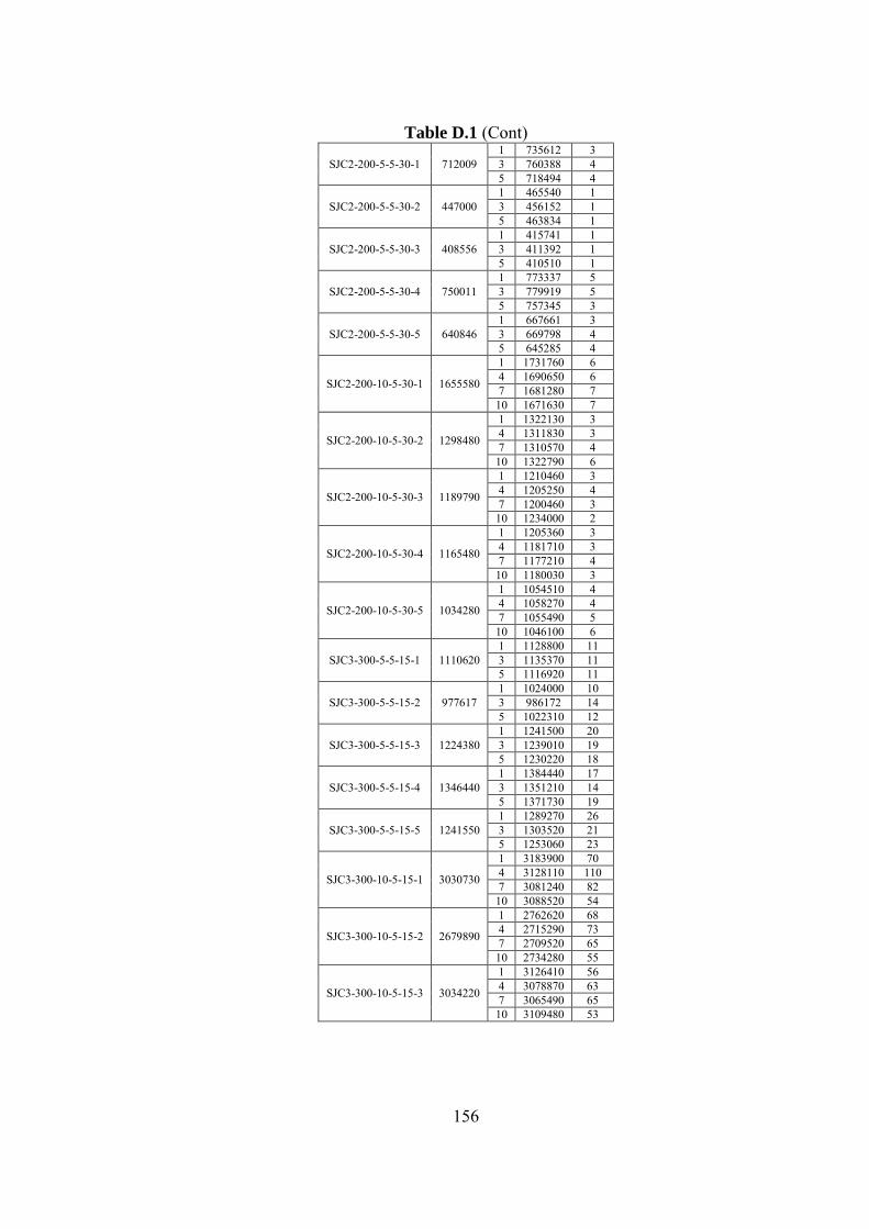
156

Table D.1 (Cont)

SJC2-200-5-5-30-1 712009 1 735612 3 3 760388 4 5 718494 4

SJC2-200-5-5-30-2 447000 1 465540 1 3 456152 1 5 463834 1

SJC2-200-5-5-30-3 408556 1 415741 1 3 411392 1 5 410510 1

SJC2-200-5-5-30-4 750011 1 773337 5 3 779919 5 5 757345 3

SJC2-200-5-5-30-5 640846 1 667661 3 3 669798 4 5 645285 4

SJC2-200-10-5-30-1 1655580

1 1731760 6 4 1690650 6 7 1681280 7

10 1671630 7

SJC2-200-10-5-30-2 1298480

1 1322130 3 4 1311830 3 7 1310570 4

10 1322790 6

SJC2-200-10-5-30-3 1189790

1 1210460 3 4 1205250 4 7 1200460 3

10 1234000 2

SJC2-200-10-5-30-4 1165480

1 1205360 3 4 1181710 3 7 1177210 4

10 1180030 3

SJC2-200-10-5-30-5 1034280

1 1054510 4 4 1058270 4 7 1055490 5

10 1046100 6

SJC3-300-5-5-15-1 1110620 1 1128800 11 3 1135370 11 5 1116920 11

SJC3-300-5-5-15-2 977617 1 1024000 10 3 986172 14 5 1022310 12

SJC3-300-5-5-15-3 1224380 1 1241500 20 3 1239010 19 5 1230220 18

SJC3-300-5-5-15-4 1346440 1 1384440 17 3 1351210 14 5 1371730 19

SJC3-300-5-5-15-5 1241550 1 1289270 26 3 1303520 21 5 1253060 23

SJC3-300-10-5-15-1 3030730

1 3183900 70 4 3128110 110 7 3081240 82

10 3088520 54

SJC3-300-10-5-15-2 2679890

1 2762620 68 4 2715290 73 7 2709520 65

10 2734280 55

SJC3-300-10-5-15-3 3034220

1 3126410 56 4 3078870 63 7 3065490 65

10 3109480 53

157

Table D.1 (Cont)

SJC3-300-10-5-15-4 3311880

1 3399920 81 4 3372340 103 7 3381430 70

10 3394020 101

SJC3-300-10-5-15-5 2809930

1 2864550 45 4 2881620 48 7 2821610 46

10 2848320 62

SJC3-300-5-5-30-1 581092 1 596739 3 3 596932 3 5 588201 3

SJC3-300-5-5-30-2 610611 1 658476 5 3 641741 6 5 627662 2

SJC3-300-5-5-30-3 791799 1 829448 7 3 800169 6 5 807957 6

SJC3-300-5-5-30-4 772712 1 821055 7 3 784653 8 5 803024 7

SJC3-300-5-5-30-5 971093 1 1025750 13 3 1003630 13 5 988710 15

SJC3-300-10-5-30-1 2303930

1 2353230 45 4 2342810 45 7 2355130 44

10 2358570 37

SJC3-300-10-5-30-2 2031090

1 2061750 34 4 2059660 31 7 2058310 34

10 2067840 48

SJC3-300-10-5-30-3 2482630

1 2541900 53 4 2517920 48 7 2503040 48

10 2506120 48

SJC3-300-10-5-30-4 2129420

1 2201950 34 4 2169730 35 7 2157960 33

10 2169400 36

SJC3-300-10-5-30-5 1704590

1 1744650 20 4 1725930 21 7 1725830 20

10 1735390 17

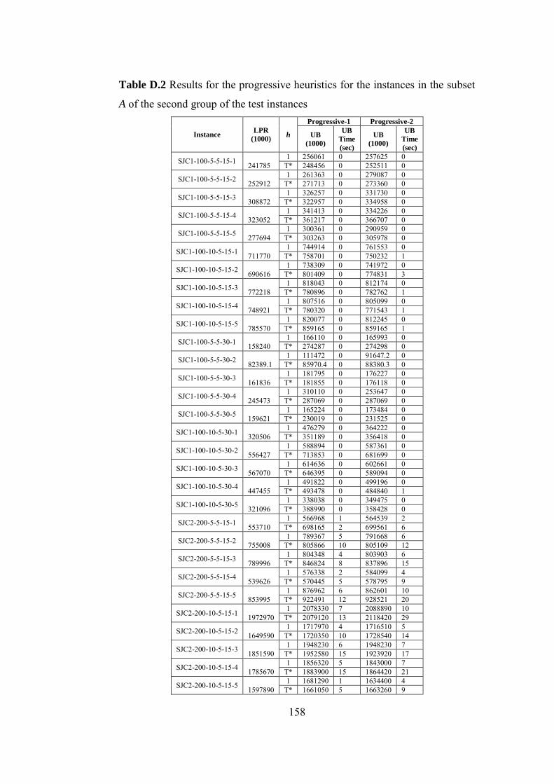
158

Table D.2 Results for the progressive heuristics for the instances in the subset

A of the second group of the test instances

Instance LPR

(1000) h

Progressive-1 Progressive-2

UB

(1000)

UB

Time

(sec)

UB

(1000)

UB

Time

(sec)

SJC1-100-5-5-15-1 241785 1 256061 0 257625 0

T* 248456 0 252511 0

SJC1-100-5-5-15-2 252912 1 261363 0 279087 0

T* 271713 0 273360 0

SJC1-100-5-5-15-3 308872 1 326257 0 331730 0

T* 322957 0 334958 0

SJC1-100-5-5-15-4 323052 1 341413 0 334226 0

T* 361217 0 366707 0

SJC1-100-5-5-15-5 277694 1 300361 0 290959 0

T* 303263 0 305978 0

SJC1-100-10-5-15-1 711770 1 744914 0 761553 0

T* 758701 0 750232 1

SJC1-100-10-5-15-2 690616 1 738309 0 741972 0

T* 801409 0 774831 3

SJC1-100-10-5-15-3 772218 1 818043 0 812174 0

T* 780896 0 782762 1

SJC1-100-10-5-15-4 748921 1 807516 0 805099 0

T* 780320 0 771543 1

SJC1-100-10-5-15-5 785570 1 820077 0 812245 0

T* 859165 0 859165 1

SJC1-100-5-5-30-1 158240 1 166110 0 165993 0

T* 274287 0 274298 0

SJC1-100-5-5-30-2 82389.1 1 111472 0 91647.2 0

T* 85970.4 0 88380.3 0

SJC1-100-5-5-30-3 161836 1 181795 0 176227 0

T* 181855 0 176118 0

SJC1-100-5-5-30-4 245473 1 310110 0 253647 0

T* 287069 0 287069 0

SJC1-100-5-5-30-5 159621 1 165224 0 173484 0

T* 230019 0 231525 0

SJC1-100-10-5-30-1 320506 1 476279 0 364222 0

T* 351189 0 356418 0

SJC1-100-10-5-30-2 556427 1 588894 0 587361 0

T* 713853 0 681699 0

SJC1-100-10-5-30-3 567070 1 614636 0 602661 0

T* 646395 0 589094 0

SJC1-100-10-5-30-4 447455 1 491822 0 499196 0

T* 493478 0 484840 1

SJC1-100-10-5-30-5 321096 1 338038 0 349475 0

T* 388990 0 358428 0

SJC2-200-5-5-15-1 553710 1 566968 1 564539 2

T* 698165 2 699561 6

SJC2-200-5-5-15-2 755008 1 789367 5 791668 6

T* 805866 10 805109 12

SJC2-200-5-5-15-3 789996 1 804348 4 803903 6

T* 846824 8 837896 15

SJC2-200-5-5-15-4 539626 1 576338 2 584099 4

T* 570445 5 578795 9

SJC2-200-5-5-15-5 853995 1 876962 6 862601 10

T* 922491 12 928521 20

SJC2-200-10-5-15-1 1972970 1 2078330 7 2088890 10

T* 2079120 13 2118420 29

SJC2-200-10-5-15-2 1649590 1 1717970 4 1716510 5

T* 1720350 10 1728540 14

SJC2-200-10-5-15-3 1851590 1 1948230 6 1948230 7

T* 1952580 15 1923920 17

SJC2-200-10-5-15-4 1785670 1 1856320 5 1843000 7

T* 1883900 15 1864420 21

SJC2-200-10-5-15-5 1597890 1 1681290 1 1634400 4

T* 1661050 5 1663260 9

159

Table D.2 (Cont.) SJC2-200-5-5-30-1 712009

1 729886 4 730177 4 T* 865128 10 813023 10

SJC2-200-5-5-30-2 447000 1 471115 2 466105 2

T* 512766 3 493982 4

SJC2-200-5-5-30-3 408556 1 451521 2 446130 4

T* 438981 3 426839 6

SJC2-200-5-5-30-4 750011 1 776174 5 783878 7

T* 832786 12 835549 14

SJC2-200-5-5-30-5 640846 1 669047 5 656677 8

T* 710315 12 710315 10

SJC2-200-10-5-30-1 1655580 1 1740210 8 1743240 9

T* 1860490 20 1862190 18

SJC2-200-10-5-30-2 1298480 1 1350940 3 1401010 7

T* 1399570 14 1375210 17

SJC2-200-10-5-30-3 1189790 1 1267400 3 1299980 5

T* 1277790 6 1240470 14

SJC2-200-10-5-30-4 1165480 1 1209380 4 1208150 4

T* 1555080 5 1555810 5

SJC2-200-10-5-30-5 1034280 1 1128640 1 1102620 4

T* 1137810 4 1131500 6

SJC3-300-5-5-15-1 1110620 1 1132810 23 1151370 25

T* 1148910 34 1148910 51

SJC3-300-5-5-15-2 977617 1 1037030 11 1010560 30

T* 1001500 29 1018580 68

SJC3-300-5-5-15-3 1224380 1 1236930 31 1236930 32

T* 1243690 46 1243690 68

SJC3-300-5-5-15-4 1346440 1 1358090 37 1369190 37

T* 1397150 38 1399370 47

SJC3-300-5-5-15-5 1241550 1 1263330 44 1257180 45

T* 1315840 45 1323490 59

SJC3-300-10-5-15-1 3030730 1 3102980 36 3116530 45

T* 3526200 54 3456630 90

SJC3-300-10-5-15-2 2679890 1 2810590 35 2789170 49

T* 2790590 53 2789930 96

SJC3-300-10-5-15-3 3034220 1 3096470 40 3093040 39

T* 3103080 74 3119050 82

SJC3-300-10-5-15-4 3311880 1 3437250 45 3423730 55

T* 3459320 76 3465090 102

SJC3-300-10-5-15-5 2809930 1 2903540 19 2877900 46

T* 2912610 45 2933510 77

SJC3-300-5-5-30-1 581092 1 596280 3 619429 4

T* 605070 5 612988 10

SJC3-300-5-5-30-2 610611 1 664316 3 635833 7

T* 643792 10 647095 19

SJC3-300-5-5-30-3 791799 1 814533 7 812308 22

T* 852779 17 870398 28

SJC3-300-5-5-30-4 772712 1 805157 17 807294 20

T* 799702 12 800837 22

SJC3-300-5-5-30-5 971093 1 985224 36 982458 36

T* 1049370 43 1051310 36

SJC3-300-10-5-30-1 2303930 1 2433430 35 2424680 45

T* 2499250 45 2446540 75

SJC3-300-10-5-30-2 2031090 1 2126600 27 2107850 36

T* 2360700 45 2352080 45

SJC3-300-10-5-30-3 2482630 1 2558620 32 2548960 54

T* 2587750 58 2569360 77

SJC3-300-10-5-30-4 2129420 1 2194440 11 2201510 19

T* 2356900 22 2209960 47

SJC3-300-10-5-30-5 1704590 1 1784690 8 1813400 13

T* 1914200 18 1846480 30

160

Table D.3 Results for the myopic heuristic starting from the last period and

DBnP with different target values for the instances in the subset A of the

second group of the test instances

Instance LPR

(1000) Target

UB

(1000)

Best

(1000)

UB

Time

(sec)

Total

Time

(sec)

SJC1-100-5-5-15-1 241785 0.7 248399 241785 0 0 0.8 248399 241785 0 0 0.9 248399 241785 0 0

SJC1-100-5-5-15-2 252912 0.7 252912 252912 0 0 0.8 252912 252912 0 0 0.9 252912 252912 0 0

SJC1-100-5-5-15-3 308872 0.7 310905 308872 0 0 0.8 310905 308872 0 0 0.9 310905 308872 0 0

SJC1-100-5-5-15-4 323052 0.7 325322 323080 0 1 0.8 325322 323080 0 1 0.9 325322 323080 0 1

SJC1-100-5-5-15-5 277694 0.7 285188 277694 0 0 0.8 285188 277694 0 0 0.9 285188 277694 0 0

SJC1-100-10-5-15-1 711770 0.7 717191 711770 1 2 0.8 717191 711770 1 2 0.9 717191 711770 1 2

SJC1-100-10-5-15-2 690616 0.7 711207 690616 0 1 0.8 711207 690616 0 1 0.9 711207 690616 0 1

SJC1-100-10-5-15-3 772218 0.7 779884 772218 0 1 0.8 779884 772218 0 1 0.9 779884 772218 0 1

SJC1-100-10-5-15-4 748921 0.7 753258 750280 0 67 0.8 753258 750280 0 66 0.9 753258 750280 0 66

SJC1-100-10-5-15-5 785570 0.7 815001 785997 1 2 0.8 815001 785997 1 2 0.9 815001 785997 1 2

SJC1-100-5-5-30-1 158240 0.7 160136 158240 0 0 0.8 160136 158240 0 0 0.9 160136 158240 0 0

SJC1-100-5-5-30-2 82389.1 0.7 84189.9 82389.1 0 0 0.8 84189.9 82389.1 0 0 0.9 84189.9 82389.1 0 0

SJC1-100-5-5-30-3 161836 0.7 162394 161836 0 0 0.8 162394 161836 0 0 0.9 162394 161836 0 0

SJC1-100-5-5-30-4 245473 0.7 245975 245473 0 0 0.8 245975 245473 0 0 0.9 245975 245473 0 0

SJC1-100-5-5-30-5 159621 0.7 159621 159621 0 0 0.8 159621 159621 0 0 0.9 159621 159621 0 0

SJC1-100-10-5-30-1 320506 0.7 325766 320527 0 0 0.8 325766 320527 0 0 0.9 325766 320527 0 0

SJC1-100-10-5-30-2 556427 0.7 568519 556427 0 0 0.8 568519 556427 0 0 0.9 568519 556427 0 0

SJC1-100-10-5-30-3 567070 0.7 573818 567070 0 0 0.8 573818 567070 0 0 0.9 573818 567070 0 0

SJC1-100-10-5-30-4 447455 0.7 451264 447455 0 1 0.8 451264 447455 0 1 0.9 451264 447455 0 1

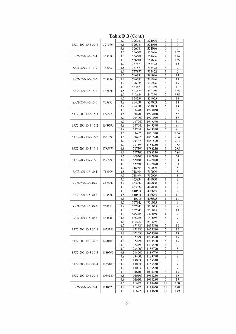
161

Table D.3 (Cont.)

SJC1-100-10-5-30-5 321096 0.7 326081 321096 0 0 0.8 326081 321096 0 0 0.9 326081 321096 0 0

SJC2-200-5-5-15-1 553710 0.7 556608 554636 2 157 0.8 556608 554636 2 174 0.9 556608 554636 2 155

SJC2-200-5-5-15-2 755008 0.7 757877 755422 3 12 0.8 757877 755422 3 9 0.9 757877 755422 3 9

SJC2-200-5-5-15-3 789996 0.7 796335 789996 5 15 0.8 796335 789996 5 15 0.9 796335 789996 5 15

SJC2-200-5-5-15-4 539626 0.7 543624 540359 2 1117 0.8 543624 540359 2 435 0.9 543624 540359 2 585

SJC2-200-5-5-15-5 853995 0.7 874330 854003 6 18 0.8 874330 854003 6 18 0.9 874330 854003 6 18

SJC2-200-10-5-15-1 1972970 0.7 1984900 1973030 9 55 0.8 1984900 1973030 9 57 0.9 1984900 1973030 9 57

SJC2-200-10-5-15-2 1649590 0.7 1687040 1649590 6 81 0.8 1687040 1649590 6 81 0.9 1687040 1649590 6 81

SJC2-200-10-5-15-3 1851590 0.7 1904870 1851590 8 234 0.8 1904870 1851590 8 234 0.9 1904870 1851590 8 234

SJC2-200-10-5-15-4 1785670 0.7 1787590 1786230 5 485 0.8 1787590 1786230 5 285 0.9 1787590 1786230 5 284

SJC2-200-10-5-15-5 1597890 0.7 1629300 1597890 5 34 0.8 1629300 1597890 5 33 0.9 1629300 1597890 5 34

SJC2-200-5-5-30-1 712009 0.7 718494 712009 4 8 0.8 718494 712009 4 8 0.9 718494 712009 4 8

SJC2-200-5-5-30-2 447000 0.7 463834 447000 1 2 0.8 463834 447000 1 2 0.9 463834 447000 1 2

SJC2-200-5-5-30-3 408556 0.7 410510 408665 1 4 0.8 410510 408665 1 11 0.9 410510 408665 1 11

SJC2-200-5-5-30-4 750011 0.7 757345 750015 3 9 0.8 757345 750015 3 9 0.9 757345 750015 3 10

SJC2-200-5-5-30-5 640846 0.7 645285 640859 4 7 0.8 645285 640859 4 7 0.9 645285 640859 4 7

SJC2-200-10-5-30-1 1655580 0.7 1671630 1655580 7 18 0.8 1671630 1655580 7 18 0.9 1671630 1655580 7 18

SJC2-200-10-5-30-2 1298480 0.7 1322790 1298580 6 15 0.8 1322790 1298580 6 15 0.9 1322790 1298580 6 21

SJC2-200-10-5-30-3 1189790 0.7 1234000 1189790 2 8 0.8 1234000 1189790 2 9 0.9 1234000 1189790 2 8

SJC2-200-10-5-30-4 1165480 0.7 1180030 1165530 3 7 0.8 1180030 1165530 3 7 0.9 1180030 1165530 3 7

SJC2-200-10-5-30-5 1034280 0.7 1046100 1034280 6 15 0.8 1046100 1034280 6 15 0.9 1046100 1034280 6 15

SJC3-300-5-5-15-1 1110620 0.7 1116920 1110620 11 149 0.8 1116920 1110620 11 148 0.9 1116920 1110620 11 149

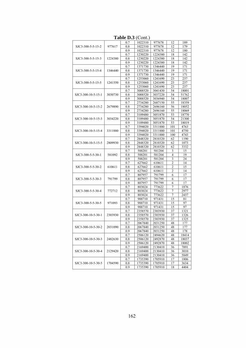
162

Table D.3 (Cont.)

SJC3-300-5-5-15-2 977617 0.7 1022310 977678 12 189 0.8 1022310 977678 12 179 0.9 1022310 977678 12 180

SJC3-300-5-5-15-3 1224380 0.7 1230220 1224380 18 142 0.8 1230220 1224380 18 142 0.9 1230220 1224380 18 142

SJC3-300-5-5-15-4 1346440 0.7 1371730 1346440 19 171 0.8 1371730 1346440 19 171 0.9 1371730 1346440 19 171

SJC3-300-5-5-15-5 1241550 0.7 1253060 1241690 23 237 0.8 1253060 1241690 23 237 0.9 1253060 1241690 23 237

SJC3-300-10-5-15-1 3030730 0.7 3088520 3041430 54 18001 0.8 3088520 3037220 54 51762 0.9 3088520 3036940 54 18007

SJC3-300-10-5-15-2 2679890 0.7 2734280 2687150 55 18359 0.8 2734280 2696160 56 18052 0.9 2734280 2696160 55 18069

SJC3-300-10-5-15-3 3034220 0.7 3109480 3051870 53 18770 0.8 3109480 3051870 54 21300 0.9 3109480 3051870 53 18019

SJC3-300-10-5-15-4 3311880 0.7 3394020 3311880 101 4763 0.8 3394020 3311880 101 4750 0.9 3394020 3311880 100 4743

SJC3-300-10-5-15-5 2809930 0.7 2848320 2810320 62 1190 0.8 2848320 2810320 62 1073 0.9 2848320 2810320 62 3332

SJC3-300-5-5-30-1 581092 0.7 588201 581204 3 15 0.8 588201 581204 4 19 0.9 588201 581204 3 24

SJC3-300-5-5-30-2 610611 0.7 627662 610611 2 14 0.8 627662 610611 2 15 0.9 627662 610611 2 14

SJC3-300-5-5-30-3 791799 0.7 807957 791799 6 17 0.8 807957 791799 6 17 0.9 807957 791799 6 17

SJC3-300-5-5-30-4 772712 0.7 803024 773622 7 1876 0.8 803024 773622 7 2977 0.9 803024 773622 7 2437

SJC3-300-5-5-30-5 971093 0.7 988710 971431 15 81 0.8 988710 971431 15 97 0.9 988710 971431 15 97

SJC3-300-10-5-30-1 2303930 0.7 2358570 2303930 37 1321 0.8 2358570 2303930 37 1326 0.9 2358570 2303930 37 1325

SJC3-300-10-5-30-2 2031090 0.7 2067840 2031250 48 177 0.8 2067840 2031250 48 177 0.9 2067840 2031250 48 178

SJC3-300-10-5-30-3 2482630 0.7 2506120 2494620 48 18414 0.8 2506120 2492870 48 18037 0.9 2506120 2492870 48 18002

SJC3-300-10-5-30-4 2129420 0.7 2169400 2130410 36 7891 0.8 2169400 2130410 36 3010 0.9 2169400 2130410 36 5849

SJC3-300-10-5-30-5 1704590 0.7 1735390 1705910 17 1806 0.8 1735390 1705910 17 3634 0.9 1735390 1705910 18 4404

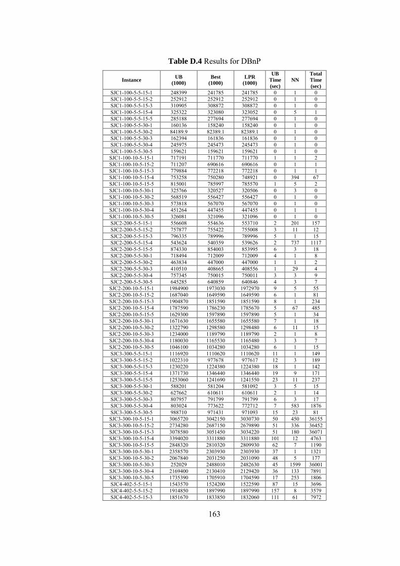
163

Table D.4 Results for DBnP

Instance UB

(1000)

Best

(1000)

LPR

(1000)

UB

Time

(sec)

NN

Total

Time

(sec)

SJC1-100-5-5-15-1 248399 241785 241785 0 1 0 SJC1-100-5-5-15-2 252912 252912 252912 0 1 0 SJC1-100-5-5-15-3 310905 308872 308872 0 1 0 SJC1-100-5-5-15-4 325322 323080 323052 0 5 1 SJC1-100-5-5-15-5 285188 277694 277694 0 1 0 SJC1-100-5-5-30-1 160136 158240 158240 0 1 0 SJC1-100-5-5-30-2 84189.9 82389.1 82389.1 0 1 0 SJC1-100-5-5-30-3 162394 161836 161836 0 1 0 SJC1-100-5-5-30-4 245975 245473 245473 0 1 0 SJC1-100-5-5-30-5 159621 159621 159621 0 1 0 SJC1-100-10-5-15-1 717191 711770 711770 1 1 2 SJC1-100-10-5-15-2 711207 690616 690616 0 1 1 SJC1-100-10-5-15-3 779884 772218 772218 0 1 1 SJC1-100-10-5-15-4 753258 750280 748921 0 394 67 SJC1-100-10-5-15-5 815001 785997 785570 1 5 2 SJC1-100-10-5-30-1 325766 320527 320506 0 3 0 SJC1-100-10-5-30-2 568519 556427 556427 0 1 0 SJC1-100-10-5-30-3 573818 567070 567070 0 1 0 SJC1-100-10-5-30-4 451264 447455 447455 0 1 1 SJC1-100-10-5-30-5 326081 321096 321096 0 1 0 SJC2-200-5-5-15-1 556608 554636 553710 2 201 157 SJC2-200-5-5-15-2 757877 755422 755008 3 11 12 SJC2-200-5-5-15-3 796335 789996 789996 5 1 15 SJC2-200-5-5-15-4 543624 540359 539626 2 737 1117 SJC2-200-5-5-15-5 874330 854003 853995 6 3 18 SJC2-200-5-5-30-1 718494 712009 712009 4 1 8 SJC2-200-5-5-30-2 463834 447000 447000 1 1 2 SJC2-200-5-5-30-3 410510 408665 408556 1 29 4 SJC2-200-5-5-30-4 757345 750015 750011 3 3 9 SJC2-200-5-5-30-5 645285 640859 640846 4 3 7 SJC2-200-10-5-15-1 1984900 1973030 1972970 9 5 55 SJC2-200-10-5-15-2 1687040 1649590 1649590 6 1 81 SJC2-200-10-5-15-3 1904870 1851590 1851590 8 1 234 SJC2-200-10-5-15-4 1787590 1786230 1785670 5 67 485 SJC2-200-10-5-15-5 1629300 1597890 1597890 5 1 34 SJC2-200-10-5-30-1 1671630 1655580 1655580 7 1 18 SJC2-200-10-5-30-2 1322790 1298580 1298480 6 11 15 SJC2-200-10-5-30-3 1234000 1189790 1189790 2 1 8 SJC2-200-10-5-30-4 1180030 1165530 1165480 3 3 7 SJC2-200-10-5-30-5 1046100 1034280 1034280 6 1 15 SJC3-300-5-5-15-1 1116920 1110620 1110620 11 1 149 SJC3-300-5-5-15-2 1022310 977678 977617 12 3 189 SJC3-300-5-5-15-3 1230220 1224380 1224380 18 1 142 SJC3-300-5-5-15-4 1371730 1346440 1346440 19 9 171 SJC3-300-5-5-15-5 1253060 1241690 1241550 23 11 237 SJC3-300-5-5-30-1 588201 581204 581092 3 5 15 SJC3-300-5-5-30-2 627662 610611 610611 2 1 14 SJC3-300-5-5-30-3 807957 791799 791799 6 3 17 SJC3-300-5-5-30-4 803024 773622 772712 7 583 1876 SJC3-300-5-5-30-5 988710 971431 971093 15 23 81 SJC3-300-10-5-15-1 3065720 3042150 3030730 50 450 36155 SJC3-300-10-5-15-2 2734280 2687150 2679890 51 336 36452 SJC3-300-10-5-15-3 3078580 3051450 3034220 51 180 36071 SJC3-300-10-5-15-4 3394020 3311880 3311880 101 12 4763 SJC3-300-10-5-15-5 2848320 2810320 2809930 62 7 1190 SJC3-300-10-5-30-1 2358570 2303930 2303930 37 1 1321 SJC3-300-10-5-30-2 2067840 2031250 2031090 48 5 177 SJC3-300-10-5-30-3 252029 2488010 2482630 45 1599 36001 SJC3-300-10-5-30-4 2169400 2130410 2129420 36 133 7891 SJC3-300-10-5-30-5 1735390 1705910 1704590 17 253 1806 SJC4-402-5-5-15-1 1543570 1524200 1522590 87 15 3696 SJC4-402-5-5-15-2 1914850 1897990 1897990 157 8 3579 SJC4-402-5-5-15-3 1851670 1833850 1832060 111 61 7972

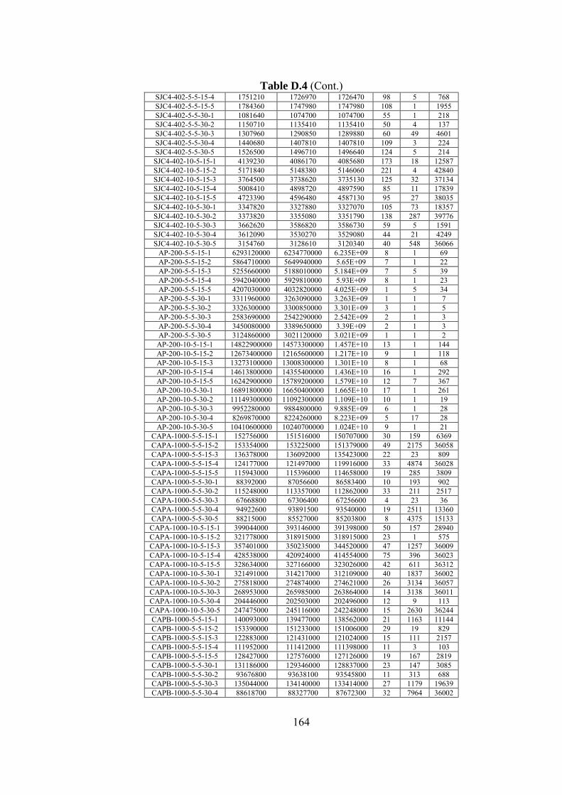
164

Table D.4 (Cont.) SJC4-402-5-5-15-4 1751210 1726970 1726470 98 5 768 SJC4-402-5-5-15-5 1784360 1747980 1747980 108 1 1955 SJC4-402-5-5-30-1 1081640 1074700 1074700 55 1 218 SJC4-402-5-5-30-2 1150710 1135410 1135410 50 4 137 SJC4-402-5-5-30-3 1307960 1290850 1289880 60 49 4601 SJC4-402-5-5-30-4 1440680 1407810 1407810 109 3 224 SJC4-402-5-5-30-5 1526500 1496710 1496640 124 5 214 SJC4-402-10-5-15-1 4139230 4086170 4085680 173 18 12587 SJC4-402-10-5-15-2 5171840 5148380 5146060 221 4 42840 SJC4-402-10-5-15-3 3764500 3738620 3735130 125 32 37134 SJC4-402-10-5-15-4 5008410 4898720 4897590 85 11 17839 SJC4-402-10-5-15-5 4723390 4596480 4587130 95 27 38035 SJC4-402-10-5-30-1 3347820 3327880 3327070 105 73 18357 SJC4-402-10-5-30-2 3373820 3355080 3351790 138 287 39776 SJC4-402-10-5-30-3 3662620 3586820 3586730 59 5 1591 SJC4-402-10-5-30-4 3612090 3530270 3529080 44 21 4249 SJC4-402-10-5-30-5 3154760 3128610 3120340 40 548 36066

AP-200-5-5-15-1 6293120000 6234770000 6.235E+09 8 1 69 AP-200-5-5-15-2 5864710000 5649940000 5.65E+09 7 1 22 AP-200-5-5-15-3 5255660000 5188010000 5.184E+09 7 5 39 AP-200-5-5-15-4 5942040000 5929810000 5.93E+09 8 1 23 AP-200-5-5-15-5 4207030000 4032820000 4.025E+09 1 5 34 AP-200-5-5-30-1 3311960000 3263090000 3.263E+09 1 1 7 AP-200-5-5-30-2 3326300000 3300850000 3.301E+09 3 1 5 AP-200-5-5-30-3 2583690000 2542290000 2.542E+09 2 1 3 AP-200-5-5-30-4 3450080000 3389650000 3.39E+09 2 1 3 AP-200-5-5-30-5 3124860000 3021120000 3.021E+09 1 1 2 AP-200-10-5-15-1 14822900000 14573300000 1.457E+10 13 1 144 AP-200-10-5-15-2 12673400000 12165600000 1.217E+10 9 1 118 AP-200-10-5-15-3 13273100000 13008300000 1.301E+10 8 1 68 AP-200-10-5-15-4 14613800000 14355400000 1.436E+10 16 1 292 AP-200-10-5-15-5 16242900000 15789200000 1.579E+10 12 7 367 AP-200-10-5-30-1 16891800000 16650400000 1.665E+10 17 1 261 AP-200-10-5-30-2 11149300000 11092300000 1.109E+10 10 1 19 AP-200-10-5-30-3 9952280000 9884800000 9.885E+09 6 1 28 AP-200-10-5-30-4 8269870000 8224260000 8.223E+09 5 17 28 AP-200-10-5-30-5 10410600000 10240700000 1.024E+10 9 1 21

CAPA-1000-5-5-15-1 152756000 151516000 150707000 30 159 6369 CAPA-1000-5-5-15-2 153354000 153225000 151379000 49 2175 36058 CAPA-1000-5-5-15-3 136378000 136092000 135423000 22 23 809 CAPA-1000-5-5-15-4 124177000 121497000 119916000 33 4874 36028 CAPA-1000-5-5-15-5 115943000 115396000 114658000 19 285 3809 CAPA-1000-5-5-30-1 88392000 87056600 86583400 10 193 902 CAPA-1000-5-5-30-2 115248000 113357000 112862000 33 211 2517 CAPA-1000-5-5-30-3 67668800 67306400 67256600 4 23 36 CAPA-1000-5-5-30-4 94922600 93891500 93540000 19 2511 13360 CAPA-1000-5-5-30-5 88215000 85527000 85203800 8 4375 15133 CAPA-1000-10-5-15-1 399044000 393146000 391398000 50 157 28940 CAPA-1000-10-5-15-2 321778000 318915000 318915000 23 1 575 CAPA-1000-10-5-15-3 357401000 350235000 344520000 47 1257 36009 CAPA-1000-10-5-15-4 428538000 420924000 414554000 75 396 36023 CAPA-1000-10-5-15-5 328634000 327166000 323026000 42 611 36312 CAPA-1000-10-5-30-1 321491000 314217000 312109000 40 1837 36002 CAPA-1000-10-5-30-2 275818000 274874000 274621000 26 3134 36057 CAPA-1000-10-5-30-3 268953000 265985000 263864000 14 3138 36011 CAPA-1000-10-5-30-4 204446000 202503000 202496000 12 9 113 CAPA-1000-10-5-30-5 247475000 245116000 242248000 15 2630 36244 CAPB-1000-5-5-15-1 140093000 139477000 138562000 21 1163 11144 CAPB-1000-5-5-15-2 153390000 151233000 151006000 29 19 829 CAPB-1000-5-5-15-3 122883000 121431000 121024000 15 111 2157 CAPB-1000-5-5-15-4 111952000 111412000 111398000 11 3 103 CAPB-1000-5-5-15-5 128427000 127576000 127126000 19 167 2819 CAPB-1000-5-5-30-1 131186000 129346000 128837000 23 147 3085 CAPB-1000-5-5-30-2 93676800 93638100 93545800 11 313 688 CAPB-1000-5-5-30-3 135044000 134140000 133414000 27 1179 19639 CAPB-1000-5-5-30-4 88618700 88327700 87672300 32 7964 36002

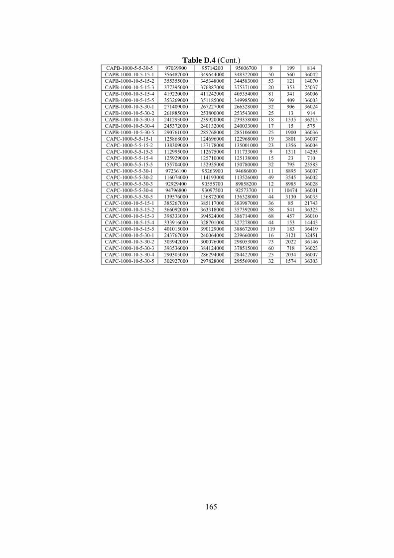
165

Table D.4 (Cont.) CAPB-1000-5-5-30-5 97039900 95714200 95606700 9 199 814

CAPB-1000-10-5-15-1 356487000 349644000 348322000 50 560 36042 CAPB-1000-10-5-15-2 355355000 345348000 344583000 53 121 14070 CAPB-1000-10-5-15-3 377395000 376887000 375371000 20 353 25037 CAPB-1000-10-5-15-4 419220000 411242000 405354000 81 341 36006 CAPB-1000-10-5-15-5 353269000 351185000 349985000 39 409 36003 CAPB-1000-10-5-30-1 271409000 267227000 266328000 32 906 36024 CAPB-1000-10-5-30-2 261885000 253800000 253543000 25 13 914 CAPB-1000-10-5-30-3 241293000 239920000 239358000 18 1535 36215 CAPB-1000-10-5-30-4 245372000 240132000 240033000 17 15 575 CAPB-1000-10-5-30-5 290761000 285768000 285106000 25 1900 36036 CAPC-1000-5-5-15-1 125868000 124696000 122968000 19 3801 36007 CAPC-1000-5-5-15-2 138309000 137178000 135001000 23 1356 36004 CAPC-1000-5-5-15-3 112995000 112675000 111733000 9 1311 14295 CAPC-1000-5-5-15-4 125929000 125710000 125138000 15 23 710 CAPC-1000-5-5-15-5 155704000 152955000 150780000 32 795 25583 CAPC-1000-5-5-30-1 97236100 95263900 94686000 11 8895 36007 CAPC-1000-5-5-30-2 116074000 114193000 113526000 49 3545 36002 CAPC-1000-5-5-30-3 92929400 90555700 89858200 12 8985 36028 CAPC-1000-5-5-30-4 94796800 93097500 92573700 11 10474 36001 CAPC-1000-5-5-30-5 139576000 136872000 136328000 44 3130 36035

CAPC-1000-10-5-15-1 385267000 385117000 383987000 36 85 21743 CAPC-1000-10-5-15-2 366092000 363318000 357392000 58 541 36323 CAPC-1000-10-5-15-3 398333000 394524000 386714000 68 457 36010 CAPC-1000-10-5-15-4 333916000 328701000 327278000 44 153 14443 CAPC-1000-10-5-15-5 401015000 390129000 388672000 119 183 36419 CAPC-1000-10-5-30-1 243767000 240064000 239660000 16 3121 32451 CAPC-1000-10-5-30-2 303942000 300076000 298053000 73 2022 36146 CAPC-1000-10-5-30-3 393536000 384124000 378515000 60 718 36023 CAPC-1000-10-5-30-4 290305000 286294000 284422000 25 2034 36007 CAPC-1000-10-5-30-5 302927000 297828000 295569000 32 1574 36303

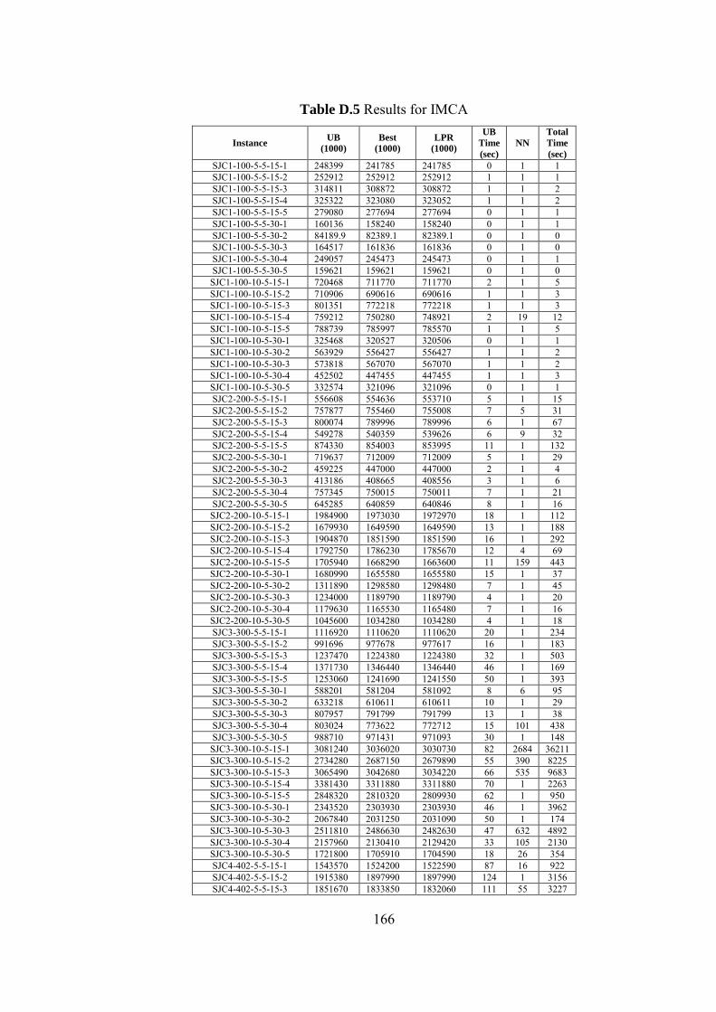
166

Table D.5 Results for IMCA

Instance UB

(1000)

Best

(1000)

LPR

(1000)

UB

Time

(sec)

NN

Total

Time

(sec)

SJC1-100-5-5-15-1 248399 241785 241785 0 1 1 SJC1-100-5-5-15-2 252912 252912 252912 1 1 1 SJC1-100-5-5-15-3 314811 308872 308872 1 1 2 SJC1-100-5-5-15-4 325322 323080 323052 1 1 2 SJC1-100-5-5-15-5 279080 277694 277694 0 1 1 SJC1-100-5-5-30-1 160136 158240 158240 0 1 1 SJC1-100-5-5-30-2 84189.9 82389.1 82389.1 0 1 0 SJC1-100-5-5-30-3 164517 161836 161836 0 1 0 SJC1-100-5-5-30-4 249057 245473 245473 0 1 1 SJC1-100-5-5-30-5 159621 159621 159621 0 1 0 SJC1-100-10-5-15-1 720468 711770 711770 2 1 5 SJC1-100-10-5-15-2 710906 690616 690616 1 1 3 SJC1-100-10-5-15-3 801351 772218 772218 1 1 3 SJC1-100-10-5-15-4 759212 750280 748921 2 19 12 SJC1-100-10-5-15-5 788739 785997 785570 1 1 5 SJC1-100-10-5-30-1 325468 320527 320506 0 1 1 SJC1-100-10-5-30-2 563929 556427 556427 1 1 2 SJC1-100-10-5-30-3 573818 567070 567070 1 1 2 SJC1-100-10-5-30-4 452502 447455 447455 1 1 3 SJC1-100-10-5-30-5 332574 321096 321096 0 1 1 SJC2-200-5-5-15-1 556608 554636 553710 5 1 15 SJC2-200-5-5-15-2 757877 755460 755008 7 5 31 SJC2-200-5-5-15-3 800074 789996 789996 6 1 67 SJC2-200-5-5-15-4 549278 540359 539626 6 9 32 SJC2-200-5-5-15-5 874330 854003 853995 11 1 132 SJC2-200-5-5-30-1 719637 712009 712009 5 1 29 SJC2-200-5-5-30-2 459225 447000 447000 2 1 4 SJC2-200-5-5-30-3 413186 408665 408556 3 1 6 SJC2-200-5-5-30-4 757345 750015 750011 7 1 21 SJC2-200-5-5-30-5 645285 640859 640846 8 1 16 SJC2-200-10-5-15-1 1984900 1973030 1972970 18 1 112 SJC2-200-10-5-15-2 1679930 1649590 1649590 13 1 188 SJC2-200-10-5-15-3 1904870 1851590 1851590 16 1 292 SJC2-200-10-5-15-4 1792750 1786230 1785670 12 4 69 SJC2-200-10-5-15-5 1705940 1668290 1663600 11 159 443 SJC2-200-10-5-30-1 1680990 1655580 1655580 15 1 37 SJC2-200-10-5-30-2 1311890 1298580 1298480 7 1 45 SJC2-200-10-5-30-3 1234000 1189790 1189790 4 1 20 SJC2-200-10-5-30-4 1179630 1165530 1165480 7 1 16 SJC2-200-10-5-30-5 1045600 1034280 1034280 4 1 18 SJC3-300-5-5-15-1 1116920 1110620 1110620 20 1 234 SJC3-300-5-5-15-2 991696 977678 977617 16 1 183 SJC3-300-5-5-15-3 1237470 1224380 1224380 32 1 503 SJC3-300-5-5-15-4 1371730 1346440 1346440 46 1 169 SJC3-300-5-5-15-5 1253060 1241690 1241550 50 1 393 SJC3-300-5-5-30-1 588201 581204 581092 8 6 95 SJC3-300-5-5-30-2 633218 610611 610611 10 1 29 SJC3-300-5-5-30-3 807957 791799 791799 13 1 38 SJC3-300-5-5-30-4 803024 773622 772712 15 101 438 SJC3-300-5-5-30-5 988710 971431 971093 30 1 148 SJC3-300-10-5-15-1 3081240 3036020 3030730 82 2684 36211 SJC3-300-10-5-15-2 2734280 2687150 2679890 55 390 8225 SJC3-300-10-5-15-3 3065490 3042680 3034220 66 535 9683 SJC3-300-10-5-15-4 3381430 3311880 3311880 70 1 2263 SJC3-300-10-5-15-5 2848320 2810320 2809930 62 1 950 SJC3-300-10-5-30-1 2343520 2303930 2303930 46 1 3962 SJC3-300-10-5-30-2 2067840 2031250 2031090 50 1 174 SJC3-300-10-5-30-3 2511810 2486630 2482630 47 632 4892 SJC3-300-10-5-30-4 2157960 2130410 2129420 33 105 2130 SJC3-300-10-5-30-5 1721800 1705910 1704590 18 26 354 SJC4-402-5-5-15-1 1543570 1524200 1522590 87 16 922 SJC4-402-5-5-15-2 1915380 1897990 1897990 124 1 3156 SJC4-402-5-5-15-3 1851670 1833850 1832060 111 55 3227

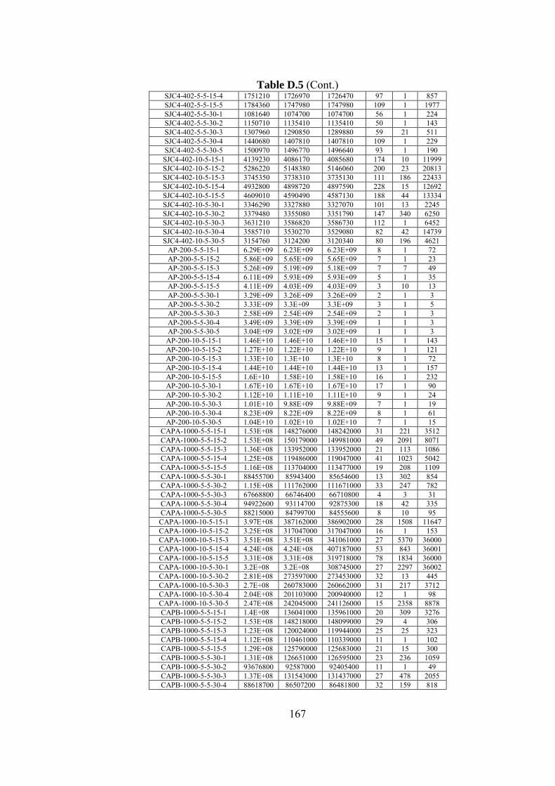
167

Table D.5 (Cont.) SJC4-402-5-5-15-4 1751210 1726970 1726470 97 1 857 SJC4-402-5-5-15-5 1784360 1747980 1747980 109 1 1977 SJC4-402-5-5-30-1 1081640 1074700 1074700 56 1 224 SJC4-402-5-5-30-2 1150710 1135410 1135410 50 1 143 SJC4-402-5-5-30-3 1307960 1290850 1289880 59 21 511 SJC4-402-5-5-30-4 1440680 1407810 1407810 109 1 229 SJC4-402-5-5-30-5 1500970 1496770 1496640 93 1 190 SJC4-402-10-5-15-1 4139230 4086170 4085680 174 10 11999 SJC4-402-10-5-15-2 5286220 5148380 5146060 200 23 20813 SJC4-402-10-5-15-3 3745350 3738310 3735130 111 186 22433 SJC4-402-10-5-15-4 4932800 4898720 4897590 228 15 12692 SJC4-402-10-5-15-5 4609010 4590490 4587130 188 44 13334 SJC4-402-10-5-30-1 3346290 3327880 3327070 101 13 2245 SJC4-402-10-5-30-2 3379480 3355080 3351790 147 340 6250 SJC4-402-10-5-30-3 3631210 3586820 3586730 112 1 6452 SJC4-402-10-5-30-4 3585710 3530270 3529080 82 42 14739 SJC4-402-10-5-30-5 3154760 3124200 3120340 80 196 4621

AP-200-5-5-15-1 6.29E+09 6.23E+09 6.23E+09 8 1 72 AP-200-5-5-15-2 5.86E+09 5.65E+09 5.65E+09 7 1 23 AP-200-5-5-15-3 5.26E+09 5.19E+09 5.18E+09 7 7 49 AP-200-5-5-15-4 6.11E+09 5.93E+09 5.93E+09 5 1 35 AP-200-5-5-15-5 4.11E+09 4.03E+09 4.03E+09 3 10 13 AP-200-5-5-30-1 3.29E+09 3.26E+09 3.26E+09 2 1 3 AP-200-5-5-30-2 3.33E+09 3.3E+09 3.3E+09 3 1 5 AP-200-5-5-30-3 2.58E+09 2.54E+09 2.54E+09 2 1 3 AP-200-5-5-30-4 3.49E+09 3.39E+09 3.39E+09 1 1 3 AP-200-5-5-30-5 3.04E+09 3.02E+09 3.02E+09 1 1 3 AP-200-10-5-15-1 1.46E+10 1.46E+10 1.46E+10 15 1 143 AP-200-10-5-15-2 1.27E+10 1.22E+10 1.22E+10 9 1 121 AP-200-10-5-15-3 1.33E+10 1.3E+10 1.3E+10 8 1 72 AP-200-10-5-15-4 1.44E+10 1.44E+10 1.44E+10 13 1 157 AP-200-10-5-15-5 1.6E+10 1.58E+10 1.58E+10 16 1 232 AP-200-10-5-30-1 1.67E+10 1.67E+10 1.67E+10 17 1 90 AP-200-10-5-30-2 1.12E+10 1.11E+10 1.11E+10 9 1 24 AP-200-10-5-30-3 1.01E+10 9.88E+09 9.88E+09 7 1 19 AP-200-10-5-30-4 8.23E+09 8.22E+09 8.22E+09 8 1 61 AP-200-10-5-30-5 1.04E+10 1.02E+10 1.02E+10 7 1 15

CAPA-1000-5-5-15-1 1.53E+08 148276000 148242000 31 221 3512 CAPA-1000-5-5-15-2 1.53E+08 150179000 149981000 49 2091 8071 CAPA-1000-5-5-15-3 1.36E+08 133952000 133952000 21 113 1086 CAPA-1000-5-5-15-4 1.25E+08 119486000 119047000 41 1023 5042 CAPA-1000-5-5-15-5 1.16E+08 113704000 113477000 19 208 1109 CAPA-1000-5-5-30-1 88455700 85943400 85654600 13 302 854 CAPA-1000-5-5-30-2 1.15E+08 111762000 111671000 33 247 782 CAPA-1000-5-5-30-3 67668800 66746400 66710800 4 3 31 CAPA-1000-5-5-30-4 94922600 93114700 92875300 18 42 335 CAPA-1000-5-5-30-5 88215000 84799700 84555600 8 10 95 CAPA-1000-10-5-15-1 3.97E+08 387162000 386902000 28 1508 11647 CAPA-1000-10-5-15-2 3.25E+08 317047000 317047000 16 1 153 CAPA-1000-10-5-15-3 3.51E+08 3.51E+08 341061000 27 5370 36000 CAPA-1000-10-5-15-4 4.24E+08 4.24E+08 407187000 53 843 36001 CAPA-1000-10-5-15-5 3.31E+08 3.31E+08 319718000 78 1834 36000 CAPA-1000-10-5-30-1 3.2E+08 3.2E+08 308745000 27 2297 36002 CAPA-1000-10-5-30-2 2.81E+08 273597000 273453000 32 13 445 CAPA-1000-10-5-30-3 2.7E+08 260783000 260662000 31 217 3712 CAPA-1000-10-5-30-4 2.04E+08 201103000 200940000 12 1 98 CAPA-1000-10-5-30-5 2.47E+08 242045000 241126000 15 2358 8878 CAPB-1000-5-5-15-1 1.4E+08 136041000 135961000 20 309 3276 CAPB-1000-5-5-15-2 1.53E+08 148218000 148099000 29 4 306 CAPB-1000-5-5-15-3 1.23E+08 120024000 119944000 25 25 323 CAPB-1000-5-5-15-4 1.12E+08 110461000 110339000 11 1 102 CAPB-1000-5-5-15-5 1.29E+08 125790000 125683000 21 15 300 CAPB-1000-5-5-30-1 1.31E+08 126651000 126595000 23 236 1059 CAPB-1000-5-5-30-2 93676800 92587000 92405400 11 1 49 CAPB-1000-5-5-30-3 1.37E+08 131543000 131437000 27 478 2055 CAPB-1000-5-5-30-4 88618700 86507200 86481800 32 159 818

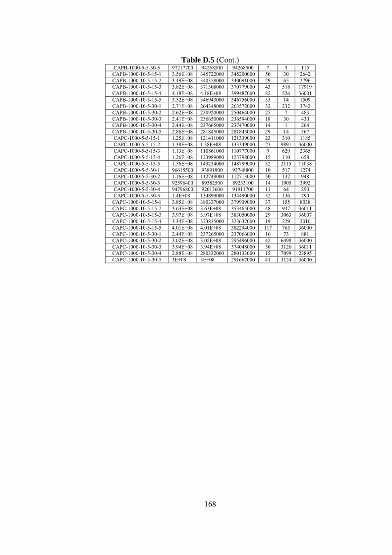
168

Table D.5 (Cont.) CAPB-1000-5-5-30-5 97217700 94268500 94268500 7 5 115

CAPB-1000-10-5-15-1 3.56E+08 345722000 345200000 50 30 2642 CAPB-1000-10-5-15-2 3.49E+08 340358000 340091000 29 65 2796 CAPB-1000-10-5-15-3 3.82E+08 371308000 370779000 43 518 17919 CAPB-1000-10-5-15-4 4.18E+08 4.18E+08 399487000 82 526 36001 CAPB-1000-10-5-15-5 3.52E+08 346943000 346756000 33 14 1509 CAPB-1000-10-5-30-1 2.71E+08 264348000 263572000 32 232 3742 CAPB-1000-10-5-30-2 2.62E+08 250920000 250464000 25 7 483 CAPB-1000-10-5-30-3 2.41E+08 236650000 236594000 18 30 430 CAPB-1000-10-5-30-4 2.44E+08 237665000 237470000 14 1 264 CAPB-1000-10-5-30-5 2.86E+08 281845000 281845000 29 14 367 CAPC-1000-5-5-15-1 1.25E+08 121411000 121339000 23 310 1185 CAPC-1000-5-5-15-2 1.38E+08 1.38E+08 133349000 23 9891 36000 CAPC-1000-5-5-15-3 1.13E+08 110861000 110777000 9 629 2365 CAPC-1000-5-5-15-4 1.26E+08 123989000 123798000 15 110 658 CAPC-1000-5-5-15-5 1.56E+08 149234000 148799000 32 2115 15038 CAPC-1000-5-5-30-1 96615500 93891900 93748800 10 517 1274 CAPC-1000-5-5-30-2 1.16E+08 112749000 112713000 50 132 948 CAPC-1000-5-5-30-3 92596400 89382500 89233100 14 1905 3992 CAPC-1000-5-5-30-4 94796800 92013600 91911700 11 64 290 CAPC-1000-5-5-30-5 1.4E+08 134899000 134490000 52 136 790

CAPC-1000-10-5-15-1 3.85E+08 380337000 379939000 37 155 8038 CAPC-1000-10-5-15-2 3.63E+08 3.63E+08 353465000 48 947 36011 CAPC-1000-10-5-15-3 3.97E+08 3.97E+08 383050000 29 3063 36007 CAPC-1000-10-5-15-4 3.34E+08 323835000 323637000 19 229 2010 CAPC-1000-10-5-15-5 4.01E+08 4.01E+08 382294000 117 765 36000 CAPC-1000-10-5-30-1 2.44E+08 237265000 237066000 16 73 881 CAPC-1000-10-5-30-2 3.02E+08 3.02E+08 295496000 42 6498 36000 CAPC-1000-10-5-30-3 3.94E+08 3.94E+08 374048000 30 3126 36011 CAPC-1000-10-5-30-4 2.88E+08 280332000 280133000 15 7099 23895 CAPC-1000-10-5-30-5 3E+08 3E+08 291667000 41 3124 36000

169

APPENDIX E

CURRICULUM VITAE

HÜSEYİN GÜDEN

BASKENT UNIVERSITY, BAGLICA CAMPUS, ANKARA, TURKEY Phone 0536 346 08 46 E-MAIL hsyngdn@baskent.edu.tr

PERSONAL

Date of Birth: 19.08.1978 Place of Birth: ÇORUM, T.R. Nationality: Turkish, Turkish Cypriot Gender: Male Marital Status: Married

EDUCATION

Ph.D. in Industrial Engineering (3.64/4 GPA) Middle East Technical University, Ankara, Turkey, 2006-present

M.S. in Industrial Engineering (3.21/4 GPA) Middle East Technical University, Ankara, Turkey, 2003-2006 Thesis Title: An Adaptive Simulated Annealing Method for Assembly Line Balancing And a Case Study Advisor: Assist. Prof. Dr. Sedef MERAL

B.S. in Industrial Engineering (3.71/4 GPA) Gazi University, Ankara, Turkey, 1998-2002

WORK EXPERIENCE

Lecturer (June 2009 – present) Baskent University, Baglıca Campus, T.R.

Research and Teaching Assistant (September 2003-June 2009) Baskent University, Baglıca Campus, T.R.

170

Production Planning Engineer (September 2002-February 2003) Nuriş Welding Machines, Sincan, Ankara, Turkey

LECTURER EXPERIENCE

One Day Project Management Course, Logistics Management School, Turkish Army, March 2009 – Present

END 202 Operations Research-I, Başkent University, 2009 Summer school, 2010 Summer school

END 301 Operations Research-II, Başkent University, 2009 Summer school

END 205 Algorithms, Başkent University, 2009-2010 Fall, 2010-2011 Fall, 2011-2012 Fall

END 401 Production Planning and Control-II, Başkent University, 2009-2010 Fall, 2010 Summer school, 2010-2011 Fall, 2011 Summer school, 2011-2012 Fall

END 310 Production Planning and Control-I, Başkent University, 2009-2010 Spring, 2010 Summer school, 2010-2011 Spring, 2011-2012 Spring

END 491 Last Year Project-I and END 492 Last Year Project-II, Başkent University, 2009-2010 Fall, 2009-2010 Spring, 2010-2011 Fall, 2010-2011 Spring, 2011-2012 Fall, 2011-2012 Spring

RESEARCH AND TEACHING ASSISTANT EXPERIENCE

END 205 Algorithms, Başkent University, 2003-2004 Fall

END 305 Statistical Analysis, Başkent University, 2003-2004 Fall

END 204 Introduction to Probability and Statistic, Başkent University 2003-2004 Spring

END 202 Operations Research-I, Başkent University, 2003-2004 Spring, 2004-2005 Spring, 2005-2006 Spring, 2006-2007 Spring

END 301 Operations Research-II, Başkent University,

171

2004-2005 Fall, 2005-2006 Fall, 2006-2007 Fall, 2007-2008 Fall

END 405 Quality Control, Başkent University, 2004-2005 Fall

END 421 Simulation Languages, Başkent University, 2004-2005 Fall

SOS 423 Human Resource Management, Başkent University, 2004-2005 Spring

END 306 Stochastic Models, Başkent University, 2004-2005 Spring, 2005-2006 Spring, 2006-2007 Spring

END 310 Production Planning and Control-I, Başkent University, 2007-2008 Spring, 2008-2009 Spring

END 401 Production Planning and Control-II, Başkent University, 2008-2009 Fall

END 491, END 492 Last Year Project, Başkent University, Every semester from 2003 to 2009

AWARDS AND HONORS

Secondary Award in Best Graduate Student Paper Competition in TRANSLOG2011 Conference. (TRANSLOG2011: A Conference on Transportation And Logistics, 15-16 June 2011, Hamilton Canada)

Ranked 2nd among 2002 graduates of Engineering and Architecture Faculty, Gazi University, Ankara, Turkey

Secondary Award in ORIE 2002 (YAEM 2002) Student Project Competition. (ORIE 2002: 22th National Conference on Operation Research and Industrial Engineering, Istanbul, Turkey)

“High Honor Certificate”, Gazi University, 1998-1999.

RESEARCH INTERESTS

Optimization Logistics Facility Location Production Planning and Scheduling Assembly Line Balancing Supply Chain Network Design Stochastic Processes Simulation

172

JOURNAL PUBLICATIONS Güden, H., Vakvak, B., Özkan, B. E., Altıparmak, F. and Dengiz, B.,2005. 'Simulation Optimization with Meta-Heuristic Algorithms: Determination of Best Kanban Numbers (Genel Amaçlı Arama Algoritmaları İle Benzetim Eniyilemesi: En İyi Kanban Sayısının Bulunması)', Journal of Industrial Engineering (Endüstri Mühendisliği

Dergisi), 16 (2), 2-15. PROCEEDINGS and/or CONFERENCE/WORKSHOP

PRESENTATIONS

Güden, H. and Meral, S., 2006. ‘Balancing Single/Multi/Mixed Model

Assembly Lines by an Adaptive Simulated Annealing Method: Solving a Real Life Case Study Problem’ ORIE2006 Kocaeli University, Turkey.

Güden, H., Pakdil, F., Vardaloğlu, Z., Hacıhasanoğlu, P. and Birlik, E., 2007. ‘Operating Room Scheduling at a University Hospital, ORIE2007 Dokuz Eylül University, Turkey.

Güden, H. and Süral, H., 2008. ‘Hub Location Problem with Non-linear Cost Fuction’, ORIE2008 Galatasaray University, Turkey.

Güden, H. and Süral, H., 2009. ‘New Complexity Results for the Hub Location Problem ’, ORIE2009 Bilkent University, Turkey.

Kara, İ., Güden, H., Öztürk, A. and Seyhan., A., 2009. ‘Computational Results for the Polynomial Size Mathematical Models for the Generalized Traveling Salesman Problem’, 10th Econometric and Statistical Symposium, Erzurum Atatürk University, Turkey.

Kara, İ., Güden, H., Seyhan., A. and Öztürk, A., 2009. ‘Integer Linear Programming Models for the Clustered Traveling Salesman Problem’, ORIE2009, Bilkent University, Turkey.

Güden, H., Süral, H. and Tağızade, E., 2010. ‘Location Problems in Speedy Train Railroad Construction’, ORIE2010, Sabancı University, Turkey.

173

Güden, H. and Süral, H., 2010. ‘A location problem in construction management’, EURO24 – 24th European Conference on Operations Research, Lisboa-Portugal.

Güden, H. and Süral, H., 2011. ‘The Depot-Quarry Location Problem and Solution Methods for It’, 12th International Econometric, Operations Research and Statistical Symposium, Denizli, Turkey.

Güden, H. and Süral, H., 2011. ‘A location problem with mobile facilities in a railroad construction project’, TRANSLOG2011 - A conference on transportation and logistics, Hamilton-Canada.

Kara, İ., Güden H. and Koç, Ö. N., 2011. ‘New polynomial Size Mathematical Models for the Generalized Traveling Salesman Problem’, PRS2011 – Production Research Symposium, İstanbul, Turkey.

LANGUAGE

English (Advanced) COMPUTER SKILLS

Programming Language: Pascal, C, C++, Visual Basic Optimization Software: CPLEX, LINDO, LINGO Simulation Software: ARENA, SIMAN Statistics Software: MINITAB, SPSS