Localization on low-order eigenvectors of data matrices

Mihai Cucuringu ∗ Michael W. Mahoney †

Abstract

Eigenvector localization refers to the situation when most of the components of an eigenvec-tor are zero or near-zero. This phenomenon has been observed on eigenvectors associated withextremal eigenvalues, and in many of those cases it can be meaningfully interpreted in termsof “structural heterogeneities” in the data. For example, the largest eigenvectors of adjacencymatrices of large complex networks often have most of their mass localized on high-degreenodes; and the smallest eigenvectors of the Laplacians of such networks are often localized onsmall but meaningful community-like sets of nodes. Here, we describe localization associatedwith low-order eigenvectors, i.e., eigenvectors corresponding to eigenvalues that are not ex-tremal but that are “buried” further down in the spectrum. Although we have observed itin several unrelated applications, this phenomenon of low-order eigenvector localization defiescommon intuitions and simple explanations, and it creates serious difficulties for the applica-bility of popular eigenvector-based machine learning and data analysis tools. After describingtwo examples where low-order eigenvector localization arises, we present a very simple modelthat qualitatively reproduces several of the empirically-observed results. This model suggestscertain coarse structural similarities among the seemingly-unrelated applications where wehave observed low-order eigenvector localization, and it may be used as a diagnostic tool tohelp extract insight from data graphs when such low-order eigenvector localization is present.

1 Introduction

The problem that motivated the work described in this paper had to do with using eigenvector-based methods to infer meaningful structure from graph-based or network-based data. Methods ofthis type are ubiquitous. For example, Principal Component Analysis and its variants have beenwidely-used historically. More recently, nonlinear-dimensionality reduction methods, spectralpartitioning methods, spectral ranking methods, etc. have been used in increasingly-sophisticatedways in machine learning and data analysis.

Although they can be applied to any data matrix, these eigenvector-based methods are gen-erally most appropriate when the data possess some sort of linear redundancy structure (in theoriginal or in some nonlinearly-transformed basis) and when there is no single data point or nosmall number of data points that are particularly important or influential [14]. The presence oflinear redundancy structure is typically quantified by the requirement that the rank of the matrixis small relative to its size, e.g., that most of the Frobenius norm of the matrix is captured bya small number of eigencomponents. The lack of a small number of particularly-influential datapoints is typically quantified by the requirement that the eigenvectors of the data matrix aredelocalized. For example, matrix coherence and statistical leverage capture this idea [8].

Localization in eigenvectors arises when most of the components of an eigenvector are zero ornear-zero [15]. (Thus, eigenvector delocalization refers to the situation when most or all of the

∗Program in Applied and Computational Mathematics, Princeton University, Princeton, NJ 08544. Email:mcucurin@math.princeton.edu†Department of Mathematics, Stanford University, Stanford, CA 94305. Email: mmahoney@cs.stanford.edu

1

arX

iv:1

109.

1355

v1 [

cs.D

M]

7 S

ep 2

011

components of an eigenvector are small and roughly the same magnitude. Below we will quantifythis idea in two different ways.) While creating serious difficulties for recently-popular eigenvector-based machine learning and data analysis methods, such a situation is far from unknown. Typi-cally, though, this phenomenon occurs on eigenvectors associated with extremal eigenvalues. Forexample, the largest eigenvectors of adjacency matrices of large complex networks often havemost of their mass localized on high-degree nodes [7]. Alternatively, the smallest eigenvectors ofthe Laplacian of such networks are often localized on small but meaningful community-like setsof nodes [17]. More generally, this phenomenon arises on extremal eigenvectors in applicationswhere extreme sparsity is coupled with randomness or quasi-randomness [12, 13, 11, 21]. In thesecases, as a rule of thumb, the localization can often be interpreted in terms of a “structuralheterogeneity,” e.g., that the degree (or coordination number) of a node is significantly higher orlower than average, in the data [12, 13, 11, 21].

In this paper, the phenomenon of localization of low-order eigenvectors in Laplacian matricesassociated with certain classes of data graphs is described for several real-world data sets andanalyzed with a simple model. By low-order eigenvectors, we mean eigenvectors associated witheigenvalues that are not extremal (in the sense of being the largest or smallest eigenvalues), butthat are “buried” further down in the eigenvalue spectrum of the data matrix. As a practicalmatter, such localization is most interesting in two cases: first, when it occurs in eigenvectorsthat are below, i.e., associated with smaller eigenvalues than, other eigenvectors that are sig-nificantly more delocalized; and second, when the localization occurs on entries or nodes thatare meaningful, e.g., that correspond to meaningful clusters or other structures in the data, to adownstream analyst.

We have observed this phenomenon of low-order eigenvector localization in several seemingly-unrelated applications (including, but not limited to, the Congress and the Migration datadiscussed in this paper, DNA single-nucleotide polymorphism data, spectral and hyperspectraldata in astronomy and other natural sciences, etc.). Moreover, based on informal discussions withboth practitioners and theorists of machine learning and data analysis, it has become clear thatthis phenomenon defies common intuitions and simple explanations. For example, the varianceassociated with these low-order eigenvectors is much less than the variance associated with “ear-lier” more-delocalized eigenvectors. Thus, these low-order eigenvectors must satisfy the globalrequirement of exact orthogonality with respect to all of the earlier delocalized eigenvectors, andthey must do so while keeping most of their components zero or near-zero in magnitude. Thisrequirement of exact orthogonality is responsible for the usefulness of eigenvector-based methodsin machine learning and data analysis, but it often leads to non-interpretable vectors—recall, e.g.,the characteristic “ringing” behavior of eigenfaces associated with low-order eigenvalues [36, 23]as well as the issues associated with eigenvector reification in the natural and social sciences [19].For this and related reasons, it is often the case that by the time that most of the variance in thedata is captured, the residual consists mostly of relatively-delocalized noise. Indeed, eigenvector-based models and methods in machine learning and data analysis typically simply assume thatthis is the case.

In this paper, our contributions are threefold: first, we will introduce the notion of low-ordereigenvector localization; second, we will describe several examples of this phenomenon in two realdata sets; and third, we will present a very simple model that qualitatively reproduces several ofthe empirical observations. Our model is a very simple two-level tensor product construction inwhich each level can be “structured” or “unstructured.” Aside from demonstrating the existenceof low-order eigenvector localization in real data, our empirical results will illustrate that mean-ingful very low variance parts of the data can—in some cases—be extracted in an unsupervisedmanner by looking at the localization properties of low-order eigenvectors. In addition, our simplemodel will suggest certain coarse structural similarities among seemingly-unrelated applications,

2

and it may be used as a diagnostic tool to help extract meaningful insight from real data graphswhen such low-order eigenvector localization is present. We will conclude the paper with a briefdiscussion of the implications of our results in a broader context.

2 Data, methods, and related work

In this section, we will provide a brief background on two classes of data where we have observedlow-order eigenvector localization, and we will describe our methods and some related work.

2.1 The two data sets we consider

The main data set we consider, which will be called the Congress data set, is a data set of rollcall voting patterns in the U.S. Senate across time [26, 38, 22]. We considered Senates in the 70th

Congress through the 110th Congress, thus covering the years 1927 to 2008. During this time, theU.S. went from 48 to 50 states, and thus the number of senators in each of these 41 Congresseswas roughly the same. After preprocessing, there were n = 735 distinct senators in these 41Congresses. We constructed an n× n adjacency matrix A, where each Aij ∈ [0, 1] represents theextent of voting agreement between legislators i and j, and where identical senators in adjacentCongresses are connected with an inter-Congress connection strength. We then considered theLaplacian matrix of this graph, constructed in the usual way; see [38] for more details.

We also report on a data set, which we will call the Migration data set, that was recently con-sidered in [10]. This contains data on county-to-county migration patterns in the U.S., constructedfrom the 2000 U.S. Census data, that reports the number of people that migrated from everycounty to every other county in the mainland U.S. during the 1995-2000 time frame [1, 30, 10].We denote by M = (Mij)1≤i,j≤N the total number of people who migrated from county i tocounty j or from county j to county i (so Mij = Mji), where N = 3107 denotes the number ofcounties in the mainland U.S.; and we let Pi denote the population of county i. We then build the

similarity matrix Wij =M2

ij

PiPjand the diagonal scaling matrix Dii =

∑Nj=1wij ; and we considered

the usual random walk matrix, D−1W , associated with this graph. We refer the reader to [10]for a discussion of variants of this similarity matrix.

2.2 The methods we will apply

In both of these applications, we will look at eigenvectors of matrices constructed from the datagraph. Recall that given a weighted graph G = (V,E,W ), one can define the Laplacian matrixas L = D −W , where W is a weighted adjacency matrix, and where D is a diagonal matrix,with ith entry Dii equal to the degree (or sum of weights) of the ith node. Then consider thesolutions to the generalized eigenvalue problem Lx = λDx. These are related to the solutionsof the eigenvalue problem Px = λx, where P = D−1W is a row-stochastic matrix that can beinterpreted as the transition matrix of a Markov chain with state space equal to the nodes inV and where Pij represents the transition probability of moving from node i to node j in onestep. In particular, if (λ, x) is an eigenvalue-eigenvector solution to Px = λx, then (1− λ, x) is asolution to Lx = λDx.

The top (resp. bottom) eigenvectors of the Markov chain (resp. generalized Laplacian eigen-value) problem define the coarsest modes of variation or slowest modes of mixing, and thus theseeigenvectors have a natural interpretation in terms of diffusions and random walks. As such,they have been widely-studied in machine learning and data analysis to perform such tasks aspartitioning, ranking, clustering, and visualizing the data [31, 29, 28, 20, 4, 9]. We are interestedin localization, not on these top eigenvectors, but on lower-order eigenvectors—for example, on

3

the 41st eigenvector (or 43rd or . . . out of a total of hundreds of eigenvectors) in the Congressdata below. (As a matter of convention, we will refer to eigenvectors that are associated witheigenvalues that are not near the top part of the spectrum of the Markov chain matrix as low-ordereigenvectors—thus, they actually correspond to larger eigenvalues in the generalized eigenvalueproblem Lx = λDx.)

We will consider several measures to quantify the idea of localization in eigenvectors as arisingwhen most of the components of an eigenvector are zero or near-zero. Perhaps most simply, wewill consider histograms of the entries of the eigenvectors. More generally, let V be a matrixconsisting of the eigenvectors of P = D−1W , ordered from top to bottom; let V (j) denote the jth

eigenvector and Vij the ith element of this jth vector; and let N =∑n

i=1 V2ij = 1. Then:

• Then the j-componentwise-statistical-leverage (CSL) of node j is an n-dimensional vectorwith ith element given by V 2

ij/N . Thus, this measure is a score over nodes that describeshow localized is a given node along a particular eigendirection.

• The j-inverse participation ratio (IPR) is the number∑n

i=1 V4ij/N . Thus, this measure is

a score over eigendirections that describes how localized is a given eigendirection.

To gain intuition for these two measures, consider their behavior in the following limiting cases. Ifthe jth eigenvector is (1/

√n, . . . , 1/

√n), i.e., is very delocalized everywhere, then every element

of the j-CSL is 1/n, and the j-IPR is 1/n. That is, they are both “small.” On the other hand, ifthe jth eigenvector is (1, 0, . . . , 0), i.e., is very localized, then the j-CSL is (1, 0, . . . , 0), and thej-IPR is 1. Thus, for both measures, higher values indicate the presence of localization, whilesmaller values indicate delocalization.

2.3 Related work in machine learning and data analysis

The j-CSL is based on the idea of statistical leverage, which has been used to characterizelocalization on the top eigenvectors in statistical data analysis [19]; while the j-IPR originated inquantum mechanics and has been applied to study localization on the top eigenvectors of complexnetworks [12]. Depending on whether one is considering the adjacency matrix or the Laplacianmatrix, localized eigenvectors have been found to correspond to structural inhomogeneities such asvery high degree nodes or very small cluster-like sets of nodes [12, 13, 11, 21, 17]. More generally,localization on the top eigenvectors often has an interpretation in terms of the “centrality” or“network value” of a node [7], two ideas which are of use in applications such as viral marketingand immunizing against infectious agents. Localization on extremal eigenvectors has also foundapplication in a wide range of problems such as distributed control and estimation problems [3]as well as asymptotic space localization in sensor networks [16].

There have been a great deal of work on clustering and community detection that rely onthe eigenvectors of graphs. Much of this work finds approximations to the best global partitionof the data [27, 29, 24, 33]. More recent work, however, has focused on local versions of theglobal spectral partitioning method [32, 2, 18]; and this work can be interpreted as partitioningwith respect to a locally-biased vector computed from a locally-biased seed set. Random walkshave been of interest in machine learning and data analysis, both because of their usefulnessin nonlinear dimensionality reduction methods such as Laplacian Eigenmaps and the relateddiffusion maps [4, 9, 5] as well as for the connections with spectral methods more generally [39,20, 25, 37]. One line of work related to this but from which ours should be differentiated has todo with looking at the smallest eigenvectors of a graph Laplacian [24, 35]. These eigenvectors arenot “buried” in the middle of the spectrum—they are associated with extremal eigenvalues andthey typically have to do with identifying bipartite structure in the graph.

4

There is a large body of work in mathematics and physics on the localization propertiesof the continuous Laplace operator, nearly all of which studies the localization properties ofeigenfunctions associated with extremal eigenvalues, and there is also a rich literature on therelationship between the spectrum and the geometry of the domain. Only recently, however, haswork advocated studying localized eigenfunctions associated to lower-order eigenvalues [15]. Alsorecently, it was noticed that low-order localization exists in two spatially-distributed networks(the Migration data we report on here and a data set of mobile phone calls between cities inBelgium) and that this localization correlated with geographically-meaningful regions [10].

3 Motivating empirical results

In this section, we will illustrate low-order eigenvector localization for the two data sets describedin Section 2, and we will show that in both cases the localization highlights interesting propertiesof the data.

3.1 Overview of empirical results

To start, consider Figure 1. This figure illustrates the IPR for several toy data sets, for Congressfor several values of the connection parameter, and for Migration. In each case, the IPR is plot-ted as a function of the rank of the corresponding eigenvector. Figure 1(a) shows this plot for adiscretization of a two-dimensional grid; and Figures 1(b) and 1(c) show this plot for a not-too-sparse Gnp random graph, where Gnp refers to the Erdos-Renyi random graph model on somenumber n of nodes, where p is the connection probability between each pair of nodes [6]. Thesetoy synthetic graphs represent limiting cases where measure concentration occurs and where de-localized eigenvectors are known to appear. More generally, the same delocalization holds for dis-cretizations of other low-dimensional spaces, as well as low-dimensional manifolds under the usualassumptions made in machine learning, i.e., those without bad “corners” and without pathologi-cal curvature or other pathological distributional properties. Not surprisingly, similar results areseen for other similar toy data sets that have been used to validate eigenvector-based algorithmsin machine learning. Two things should be noted about these results: first, even in these idealizedcases, the IPR is not perfectly uniform, even for large values of the rank parameter, although thenonuniformity due to the random noise is relatively modest and seemingly-unstructured; and sec-ond, when the data are sparser, e.g., when the connection probability p is smaller in the randomgraph model, the nonuniformity due to noise is somewhat more pronounced.

Next, Figures 1(d), 1(e), 1(f), and 1(g) illustrate the IPR for the Congress data for severaldifferent values of the parameter defining the strength of interactions between successive Con-gresses, and Figure 1(h) illustrates the IPR for the Migration data. In all these cases, the IPRindicates that many of the low-order eigenvectors are significantly more localized than earliereigenvectors. Moreover, the localization is robust in the sense that similar (but often noisier)results are obtained if the details of the kernel connecting different counties is changed or if theconnection probability between individuals in successive Congresses is modified within reasonableranges. This is most prominent in the Congress data. For example, when the connection prob-ability is small, e.g., ε = 0.1, as it was in the original applications [38, 22]. there is a significantlocalization-delocalization transition talking place between the 40th and 41st eigenvector. (Thesignificance of this will be described below, but recall that the data consists of 41 Congresses. Ifthe Congress data set is artificially truncated to consist of some number of Congresses otherthan 41, then this transition would have taken place at some other location in the spectrum,and we would have illustrated those eigenvectors.) Note, however, that when the connectionparameter is increased from ε = 0.1 to ε = 1 and above, the low-order localization becomes much

5

(a) Two-dimensional grid. (b) Random graph,G(n, p = 0.01).

(c) Random graph,G(n, p = 0.03).

(d) Congress ε = 0.01

(e) Congress, ε = 0.1. (f) Congress, ε = 1. (g) Congress, ε = 10. (h) Migration data.

Figure 1: Inverse Participation Ratio (IPR), as a function of the rank of the correspondingeigendirection, for several data graphs. For grids and other well-formed low-dimensional meshesas well as for not-extremely-sparse random graphs, all eigenvectors are fairly delocalized andthe IPR is relatively flat. For Congress and Migration, there is substantial localization onlow-order eigenvectors.

less structured. In addition, unpublished results clearly indicate that in this case the structureshighlighted by the low-order localization are much more noisy and much less meaningful to thedomain scientist.

3.2 The Congress data

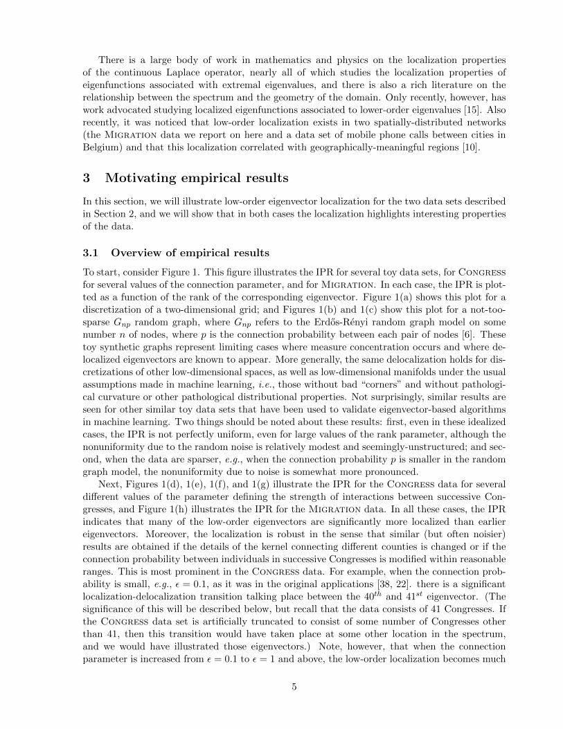
For a more detailed understanding of the localization phenomenon for the Congress data (whenε = 0.1), consider Figures 2, 3, and 4. Figure 2 presents a pictorial illustration of the top severaleigenvectors and several of the lower-order eigenvectors. (Note that the numbering starts with thefirst nontrivial eigenvector.) These particular eigenvectors have been chosen to illustrate: the topthree directions defining the coarsest modes of variation in the data; the three eigenvectors aboveand the three eigenvectors below the low-order localization-delocalization transition; and threeeigenvectors further down in the spectrum. The first three eigenvectors are fairly delocalized andexhibit global oscillatory behavior characteristic of sinusoids that might be expected for data that“looked” coarsely one-dimensional. Eigenvectors 38 to 40 are quite far down in the spectrum;interestingly, they exhibit some degree of localization, perhaps more than one would naıvelyexpect, but are still fairly delocalized relative to subsequent eigenvectors. Starting with the 41st

eigenvectors, and continuing with many more eigenvectors that are not illustrated, one sees aremarkable transition—although they are quite far down in the spectrum, these eigenvectorsexhibit a remarkable degree of localization, very often on a single Congress or a few temporally-adjacent Congresses. (Note that in these and other figures the Y-axis is often different fromsubfigure to subfigure. While creating difficulties for comparing different plots, the alternativewould involve losing the resolution along the Y-axis for all but the most localized eigenvectors.)Figure 3 shows the SLS for these twelve eigenvectors, and Figure 4 shows a histogram of the entriesfor each of these twelve eigenvectors. By both of these measures, very pronounced localization isclearly observed, complementing the observations in the previous figure.

6

Figure 2: The Congress data: illustration of several of the eigenvectors, when the inter-Congresscoupling is set to ε = 0.1. (Recall that the X-axis essentially corresponds to time.) Shown arethe top eigenvectors and several of the lower-order eigenvectors that exhibit varying degrees oflocalization.

As an illustration of the significance of the structure highlighted by these low-order eigenvec-tors, note that only 0.73% of the spectrum is captured by the 41st eigenvector and that over 99.9%of the (L2) “mass” (and 92.3% of the L1 mass) of 41st eigenvector is on individuals who servedin the 108th Congress. Similarly, only 0.42% of the spectrum is captured by the 43rd eigenvectorand 98.5% of the (L2) “mass” (and 71.7% of the L1 mass) of 43rd eigenvector is on individualswho served in the 106th Congress. Similar results are seen for many (but certainly not all) of thelow-order eigenvectors. That is, in many cases, although these low-order eigenvectors accountfor only a small fraction of the variance in the data, they are often strongly localized on a singleCongress (or, as Figure 2 illustrates, a small number of temporally-adjacent Congresses), i.e.,at a single time step of the time series of voting data. In part because of this, these low-ordereigenvectors can in some cases be used to perform common machine learning and data analysistasks.

Consider, for example, spectral clustering, which involves partitioning the data by performinga “sweep cut” over an eigenvector computed from the data. The first eigenvector shown in Figure 2clearly illustrates that a sweep cut over the first nontrivial eigenvector of the Laplacian of thefull data set will partition the network based on time, i.e., into a temporally-earlier cluster anda temporally-later cluster. Not surprisingly, low-order eigenvectors can highlight very differentstructures in the data. For example, by performing a sweep cut over the first nontrivial eigenvectorof the Laplacian of the subnetwork induced by the nodes in the 110th Congress, one obtainsthe same partition (basically, a partition along party lines [26, 38, 22]) as when the sweep cutis performed on the 41st eigenvector of the Laplacian of the full data set. This is illustratedin Figure 5. Clearly, there is a strong correlation, as that low-order eigenvector is effectivelyfinding the partition of the 110th Congress into two parties. (Indeed, the color-coding in Figure 2

7

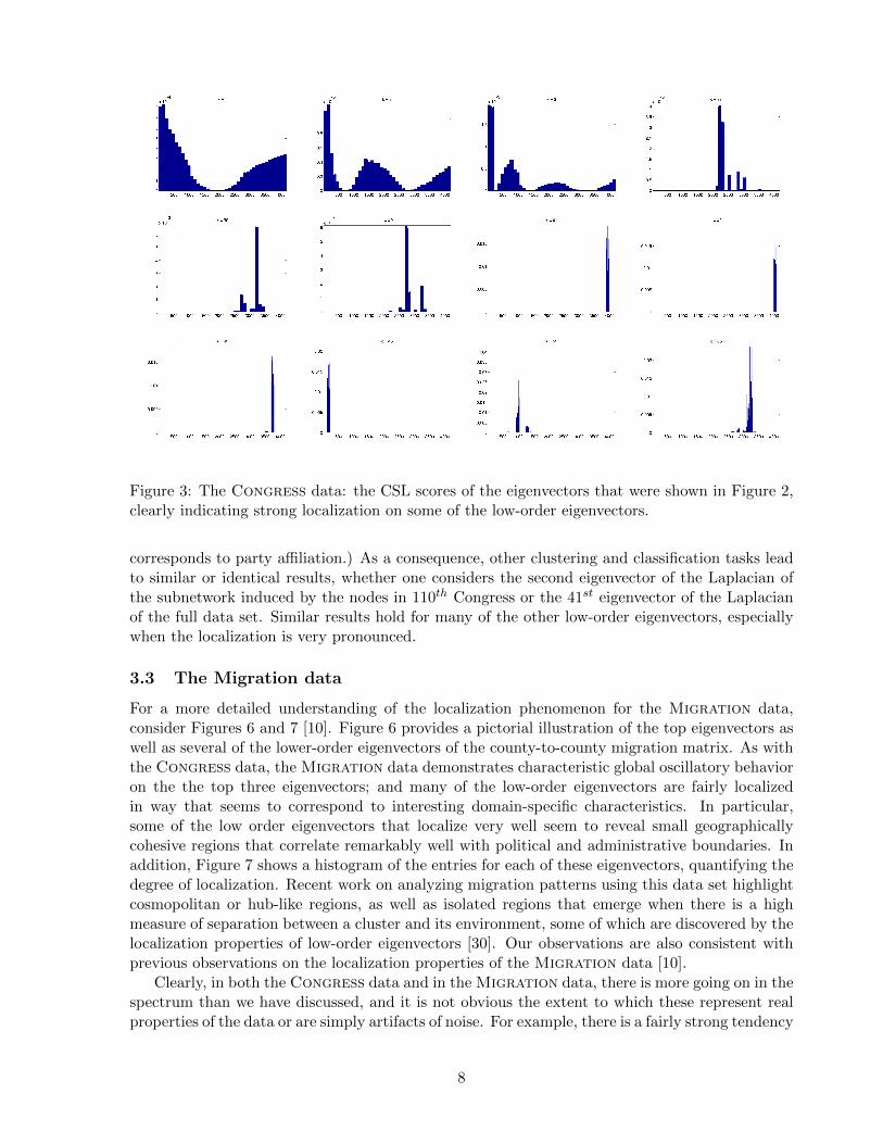
Figure 3: The Congress data: the CSL scores of the eigenvectors that were shown in Figure 2,clearly indicating strong localization on some of the low-order eigenvectors.

corresponds to party affiliation.) As a consequence, other clustering and classification tasks leadto similar or identical results, whether one considers the second eigenvector of the Laplacian ofthe subnetwork induced by the nodes in 110th Congress or the 41st eigenvector of the Laplacianof the full data set. Similar results hold for many of the other low-order eigenvectors, especiallywhen the localization is very pronounced.

3.3 The Migration data

For a more detailed understanding of the localization phenomenon for the Migration data,consider Figures 6 and 7 [10]. Figure 6 provides a pictorial illustration of the top eigenvectors aswell as several of the lower-order eigenvectors of the county-to-county migration matrix. As withthe Congress data, the Migration data demonstrates characteristic global oscillatory behavioron the the top three eigenvectors; and many of the low-order eigenvectors are fairly localizedin way that seems to correspond to interesting domain-specific characteristics. In particular,some of the low order eigenvectors that localize very well seem to reveal small geographicallycohesive regions that correlate remarkably well with political and administrative boundaries. Inaddition, Figure 7 shows a histogram of the entries for each of these eigenvectors, quantifying thedegree of localization. Recent work on analyzing migration patterns using this data set highlightcosmopolitan or hub-like regions, as well as isolated regions that emerge when there is a highmeasure of separation between a cluster and its environment, some of which are discovered by thelocalization properties of low-order eigenvectors [30]. Our observations are also consistent withprevious observations on the localization properties of the Migration data [10].

Clearly, in both the Congress data and in the Migration data, there is more going on in thespectrum than we have discussed, and it is not obvious the extent to which these represent realproperties of the data or are simply artifacts of noise. For example, there is a fairly strong tendency

8

Figure 4: The Congress data: histograms of the entries of the eigenvectors that were shown inFigure 2, clearly indicating strong localization on some of the low-order eigenvectors.

in the Congress data for localization to occur on very early Congresses or very late Congresses;when this happens, there is a tendency for eigenvectors with localization on recent Congressesto account for a larger fraction of the variance of the data than eigenvectors with localizationon much older Congresses.; etc. In addition, there are also many other low-order eigenvectors inthese two data sets that are delocalized, noisy, and seemingly-meaningless in terms of the domainfrom which the data are drawn. We will discuss these and other issues below. Our point hereis simply to illustrate that there can exist a substantial degree of localization on certain low-order eigenvectors; this this localization can highlight properties of the data—temporally-localinformation such as a party-line partition of a single Congress or small geographically cohesiveregions that have experienced nontrivial migration patterns—of interest to the domain scientist;and that these properties are not highlighted among the coarsest modes of variation of the datawhen the data are viewed globally.

4 A simple model

In this section, we will describe a simple model that exhibits low-order eigenvector localization.This model qualitatively reproduces several of the results that were empirically observed in Sec-tion 3, and it can be used as a diagnostic tool to help extract insight from data graphs when suchlow-order eigenvector localization is present.

4.1 Description of the TwoLevel model

To motivate our TwoLevel model, consider what the Congress data “looks like” if one“squints” at it, i.e., in “coarse-grained” sense. In this case, most edges are between differentmembers of a single Congress, i.e., they are temporally-local at a single time-slice; and the re-

9

(a) Illustration of Congress in theform of a “spy” plot.

(b) Normalized square spectrum. (c) Partitioning based on the 41st

eigenvector.

Figure 5: First panel: A “spy” plot of the Congress data. The blocks on the diagonal correspondto the voting patterns in each of the 41 Congresses, and the off-diagonal entries take the valueε = 0.1 when a single individual served in two successive Congresses. Second panel: Barplot of the

normalized square spectrum of the Congress matrix, i.e.,λ2i∑nj=1 λ

2j, for i = 1, . . . , 100, indicating

that the low-order eigenvalues account for a relatively-small fraction of the variance in the data.

Third panel: Plot of spectral clustering based on the first nontrivial eigenvector v(1)G2006

of the

matrix G2006, where G2006 denotes the full Congress restricted to the senators from the 110th

Congress (which includes the years 2006 and 2007). If we let v(41)2006 denote the restriction of the

(localized) 41st eigenvector of full Congress data to the the senators in the 110th Congress, then

|v(1)G2006− v(41)2006| ≤ 3× 10−3, and an identical partition and plot (at the level of resultuion of this

figure) is generated by partitioning by performing a sweep cut along v(41)2006.

mainder of the edges are between a single individual in two consecutive Congresses, i.e., theyare still fairly temporally-local. That is, there is some structured graph (structured dependingon the details of the voting pattern in any particular Congress) for which the temporally-localconnections are reasonably strong (assuming that the connection parameter between individu-als in successive Congresses is not extremely small or extremely large) that is “evolving” alonga one-dimensional temporal scaffolding. Thus, if one “zooms in” and looks locally at a singleCongress, then the properties of that Congress should be apparent. For example, the best parti-tion computed from a spectral clustering algorithm for any single Congress is typically stronglycorrelated with party affiliation [26, 38, 22]. On the other hand, if one “zooms out” and looks atthe entire graph, then the linear time series structure should be apparent and the properties ofany single Congress should be less important. For example, the best partition computed from aspectral clustering algorithm for the entire data set split the data into the first temporal half andthe second temporal half and thus fails to see party affiliations.

In cases such as this, where there are two different “size scales” to the interactions, a zero-thorder model for the data may be given by the following tensor product structure. Let W bea “base graph” representing the structure of “local” interactions at local or small size scales.For example, this could be a simple model for the voting patterns within a single Congress;or this could represent the inter-county migration patterns within a single state or geopoliticalregion. In addition, let N be an “interaction model” that governs the “global” interaction betweendifferent base graphs W . For example, this could be a “banded” or “tridiagonal” matrix, in whichthe nonzero components above and below the diagonal represent the connection links betweentwo Congresses at adjacent time steps; or this could be a discretization of a low-dimensionalmanifold representing the geographical connections in a nation, if spatially-local couplings are

10

Figure 6: The Migration data: pictorial illustration of several of the eigenfunctions. Shown arethe top eigenfunctions and several of the lower-order eigenfunctions that exhibit varying degreesof localization.

most important; or this could even be a more general noise model in which edges are addedrandomly between every pair of nodes (if, e.g., the connections between different base graphs aremuch less structured, as in social and information networks [17]). Then, a simple a zero-th ordermodel, which we will denote the TwoLevel model, is given by

G = H +N , where

H = I ⊗W,

where I is the identity matrix and H = I ⊗W denotes the tensor product between I and W .In what follows, we will illustrate the properties of the TwoLevel model in several idealized

settings. To do so, we will consider the base graph W to be either “structured” or “unstructured,”and we will also consider the interaction model N to be either “structured” or “unstructured.”

• For the base graph, W , we will model the unstructured case by a single unstructured Erdos-Renyi random graph [6], Gnp, on some number n of nodes, where the connection probabilitybetween each pair of nodes is p; and we will model the structured case by a so-called 2-module. By a “2-module,” we mean two Erdos-Renyi random graphs, where intra-modulenodes are randomly connected with probability p1 and inter-module nodes are connectedwith some much lower probability p2. (This 2-module is structured in the sense that the

11

Figure 7: The Migration data: histograms of the entries of the eigenfunctions that were shownin Figure 6, clearly indicating localization on some of the low-order eigenfunctions.

top eigenvector of the 2-module graph is the Fiedler vector that would clearly separate thetwo modules.)

• For the interaction model, N , we will model structured noise as a “path graph,” i.e., atree with two or more vertices that is not branched at all and which thus has a “banded”adjacency matrix; and we will model unstructured noise by randomly connecting any twonodes in different modules with some small probability, i.e., by an Erdos-Renyi randomgraph with some small connection probability p.

Clearly, for both the base graph and for the interaction model, these are limiting cases. Forexample, rather than consider a 2-module as the base graph, one could consider a 3-module tomodel the existence of a good tri-partition of the base graph, a 4-module, etc. Similarly, ratherthan just considering interactions along a one-dimensional scaffolding, one could consider it alonga two-dimensional scaffolding, etc. Unpublished empirical results indicate that, for both the basegraph and for the interaction model, by considering these weaker forms of structure (in particular,3-modules rather than 2-modules or a two-dimensional scaffolding rather than a one-dimensionalscaffolding), we obtain results that are similar to but intermediate between the structured andunstructured results that we report below. Formalizing this more generally and understandingthe theoretical and empirical implications of perturbations of tensor product matrices is an openproblem raised by our observations.

12

4.2 Empirical properties of the TwoLevel model

Here, we will examine the behavior of the TwoLevel model for various combinations of struc-tured and unstructured graphs for the base graph and the the interaction model. Our goal willbe to reproduce qualitatively some of the properties we observed in Section 3 and to understandtheir behavior in terms of the parameters of the TwoLevel model.

To begin, Figure 8 illustrates a graph consisting of several hundred nodes organized as a “pathgraph of 2-modules”; that is, it consists of five 2-modules connected together as beads along aone-dimensional scaffolding. (All of the figures for the behavior of the TwoLevel model containa subset of: a pictorial illustration of the graph in the form of a “spy” plot; the IPR scores, asa function of the rank of the eigenvector; a barplot of the normalized square spectrum; plots ofseveral of the eigenvectors; and the corresponding statistical leverage scores. Figure 8 plots all ofthese quantities.) The first four nontrivial eigenvectors in Figure 8 are fairly constant along eachof the beads; and they exhibit the characteristic sinusoidal oscillations that one would expectfrom eigenfunctions of the Laplacian on the continuous line or a discrete path graph. The nextfive eigenvectors are much more localized; and they tend to be localized either on a single beadat the endpoints of the path or on a small number of nearby beads in the middle of the path.In addition, on the fifth and sixth eigenfunction, which are localized on a single 2-module, thereis a natural partition of that 2-module based on the sign of that eigenvector, and that partitionsplits the 2-module into the two separate modules. Later eigenvectors are still more localized thanleading-order eigenvectors, at least by the IPR measure, but they do not seem to be localized insuch a way as to yield insight into the data.

Next, Figures 9 and 10 present the same results for two modifications of this basic setup.Figure 9 does it for an “unstructured graph of 2-modules,” i.e., for five 2-modules connectedwith random interactions. In this case, low-order eigenvector localization is still present, but it ismuch less prominent by the IPR measure, and it is significantly more noisy when the eigenvectorsthemselves are visualized. Also, and not surprisingly, the situation becomes noisier still if the off-diagonal noise is increased. Figure 10 presents results for a “path graph of unstructured graphs,”i.e., several random unstructured graphs organized as beads along a one-dimensional scaffolding.Again, low-order eigenvector localization is still present, but again the situation is significantlymore noisy. Note, though, that although the localization does not lead to most of the mass onlow-order eigenvectors being localized on a single bead, there is still a tendency for localizationto occur at the endpoints of the path.

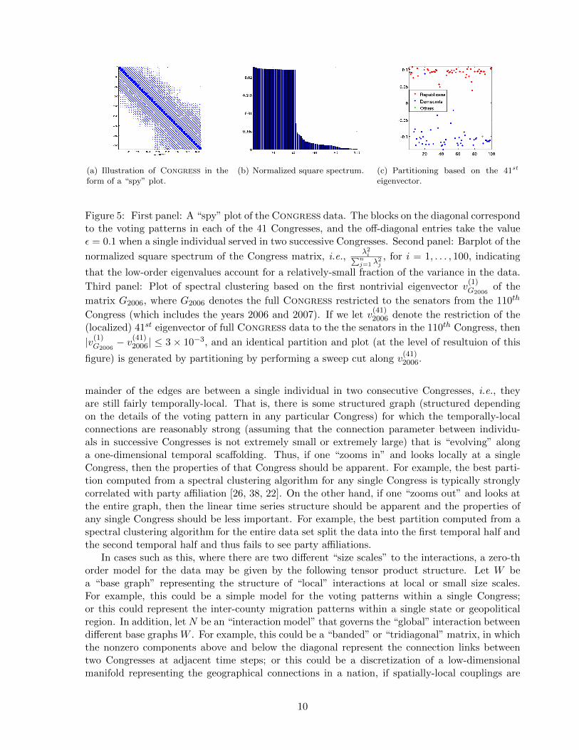
Finally, in order to understand the effect of varying the structure of the base modules on thelocalization properties of the eigenvectors, Figures 11 and 12 illustrate the situation when thebeads of the path graph are of two different types: unstructured Erdos-Renyi random graph (to bedenoted by “E”); and structured 2-modules (to be denoted by “2”). Combining beads in this wayis of interest since may be thought of as a zero-th order model of, e.g., a more-or-less polarizedCongress. The former figure illustrates the case when most of the beads are unstructured (inthe order EE2E2), while the latter illustrates the case when most of the beads are structuredand a few are less-structured (in the order 22E2E). For the EE2E2 situation, the low-ordereigenvectors highlight the two relatively more-structured 2-modules, starting with the one at theendpoint, although there is some residual structure highlighted by low-order eigenvectors on theunstructured E beads. Conversely, for the 22E2E case, the 2-modules tend to be highlighted;the E beads tend to be lost, but they do tend to make the localization on nearby 2-modules lesspronounced.

13

Figure 8: Results from the TwoLevel model, where the parameters have been set as a “pathgraph of 2-modules,” with edge densities p1 = 0.8, p2 = 0.2, and where a pair of nodes fromconsecutive 2-modules are connected with probability p = 0.05. Top left is a pictorial illustrationof the graph in the form of a “spy” plot. Top middle is the IPR scores, as a function of the rank

of the eigenvector. Top right is a barplot of the normalized square spectrum, i.e.,λ2i∑nj=1 λ

2j

for

i = 1, . . . , 65. Next two rows are the top 12 eigenvectors. Last two rows are the correspondingstatistical leverage scores.

4.3 Theoretical considerations

The empirical results on the TwoLevel model demonstrate that a very simple tensor productconstruction can shed light on some of the empirical observations for the Congress data and theMigration data that were made in Section 3. More generally, the TwoLevel model may beused as a diagnostic tool to help extract insight that is useful for a downstream analyst from datagraphs when such low-order eigenvector localization is present. To help gain insight into “why”our empirical observations hold, here we will provide some insight that is guided by theory. Adetailed theoretical understanding of the TwoLevel model is beyond the scope of this paper, asit would require a matrix perturbation analysis of the tensor product of structured matrices. Thisis a technically-involved topic, in part since a straightforward application of matrix perturbationideas tends to “wash out” the bottom part of the spectrum [34].

Instead of attempting to provide this, we will illustrate how many of the empirical results canbe “understood” as a consequence of several rules-of-thumb that are well-known to practitioners

14

Figure 9: Results from the TwoLevel model, where the parameters have been set as a “unstruc-tured graph of 2-modules,” where each 2-module W has edge densities p1 = 0.8 and p2 = 0.2, andwhere the unstructured N is a random grpah with p = 0.02. Shown are: a pictorial illustrationof the graph; the IPR scores; the normalized square spectrum; and the top 10 eigenvectors.

of eigenvector-based machine learning and data analysis tools.

• First, recall that tensor product constructions lead to separable eigenstates. In particular,for the TwoLevel model, the spectrum of H is related in a simple way to those of I andW : its eigenvalues are just the direct products of the eigenvalues of I and W , and thecorresponding eigenvectors of W are the tensor products of the eigenvectors of I and W .For example, if 1 and v1 are the top eigenvalue/eigenvector of I, and 5 and u1 of W , thenthe eigenvector of W corresponding to the top eigenvalue 1⊗5 = 5 is (v1)⊗ (u1); and so on.Assuming that the perturbation caused by the interaction model N is “sufficiently weak”relative to the base graph W , this suggests two things: first, that the top eigenvectors ofthe full graph will not “see” the internal structure of the base graph W ; second, that thenumber of these top eigenvectors will equal the number of base graphs (minus one, if thetrivial eigenvector is not counted); and third, that properties of the eigenvectors of the basegraph W may manifest themselves in subsequent low-order eigenvectors of the full graph.All of these phenomena are clearly observed in the empirical results for the TwoLevel, aswell as for the Congress data when the inter-Congress couplings are small to moderate.When the inter-Congress couplings become larger, the interaction model is less weak, inwhich case the situation is much noisier and more complex. Similarly, for the Migrationdata, there is some geographically-local structure illustrated in the low-order eigenvectors,but the situation is much noisier, suggesting that the interaction model N is more complexor that a simple separation of scales in a tensor product construction is less appropriate forthese data.

• Second, recall that eigenvectors have strong connections with diffusions. For example, the

15

Figure 10: Results from the TwoLevel model, where the parameters have been set as an “pathgraph of unstructured graphs,” where each base graph W is a random graph G(n = 100, p = 0.2),and where a pair of nodes from consecutive base graphs are connected with probability 0.01.Shown are: a pictorial illustration of the graph; the IPR scores; the normalized square spectrum;and the top 10 eigenvectors.

power method can be used to compute the top eigenvector of certain matrices, and randomwalks can be used to compute vectors which find good partitions of the data. Empiricalresults on the TwoLevel data illustrate that when the base graph W is structured (a2-module with a good bipartition, as opposed to an unstructured random graph) and/orwhen the interaction model N is structured (a path graph, as opposed to an unstructuredrandom graph) then the low-order localization is most pronounced. (This may be seen asa consequence of the implicit “isoperimetric capacity control” associated with diffusing invery low-dimension spaces or when there are very good bipartitions of the data. Formalizingthese trade-offs would provide a precise but nontrivial sense in which perturbation causedby the interaction model N is “sufficiently weak” relative to the base graph W .) Relatedly,below the localization-delocalization transition, there is a fairly strong tendency in theCongress data for localization to occur on very early Congresses or very late Congresses,i.e., at early or late but not at intermediate times. A similar but somewhat weaker tendencyis seen for localization to occur in the Migration data at the boundaries or geographicborders of the data, suggesting that an explanation for this has to do with random walks“getting stuck” at “corners” of the configuration space. Relatedly, in the Congress data,on low-order eigenvectors for which the localization is somewhat less pronounced, there isoften but not always substantial mass on several temporally-adjacent Congresses.

• Third, recall that higher-variance eigenvectors occur earlier in the spectrum. As a conse-quence of this, the conventional wisdom is that the top eigenvector is relatively smooth andthat subsequent eigenvectors exhibit characteristic higher-frequency sinusoidal oscillations;and, indeed, this is observed in both the real and synthetic data. More interestingly, one

16

Figure 11: Results from the TwoLevel model, with two different types base graphs organizedas a path graph; the order of the base graphs is EE2E2. Each “2” has edge densities p1 = 0.8and p2 = 0.2; each “E” is a random graph with p to match the edge densities inside the beads;and nodes between successive beads are connected with probability 0.05. Shown are: a pictorialillustration of the graph; the IPR scores; the normalized square spectrum; and the 5th through9th eigenvectors.

should observe that in the Congress data, eigenvectors with localization on recent, i.e.,temporally-later, Congresses tend to occur earlier in the spectrum, i.e., account for a largerfraction of the variance, than eigenvectors with localization on much older Congresses. Anexplanation for this is given by the observation that more recent Congresses are substantiallymore “polarized” than earlier Congresses [26, 38, 22]. Since the variance associated with amore polarized base graph should be larger than that associated with a less polarized basegraph, one would expect that (assuming that eigenvectors with localization on both earlierand on later Congresses are observed in the data) eigenvectors with localization on recent(and thus more polarized) Congresses should be seen before eigenvectors with localizationon older (and less polarized) Congresses. This explanation is given clear support by consid-ering the order in which localized low-order eigenvectors appear when more-structured andless-structured base graphs are combined; see Figures 11 and 12.

• Fourth, recall that lower-order eigenvectors are exactly orthogonal to earlier eigenvectors.Since the requirement of exact orthogonality is typically unrelated to the processes gen-erating the data, this often manifests itself in denser eigenvectors that often have weakerlocalization properties and that are largely uninterpretable in terms of the domain fromwhich the data are drawn. This is the conventional wisdom, and (although not presentedpictorially) this is also seen in some of the lower-order eigenvectors in the data sets we havebeen discussing.

Although these rule-of-thumb principles do not explain everything that a rigorous perturbationanalysis of the tensor product of structured matrices might hope to provide, they do help tounderstand many of the observed empirical results that are seemingly arbitrary or simply artifactsof noise in the data. In addition, they can be used to understand the properties of eigenvector-based methods more generally. As a trivial example, recall that the Congress data from Section 3was for a time period when the number of U.S. states and thus U.S. senators did not change

17

Figure 12: Results from the TwoLevel model, with two different types base graphs organizedas a path graph; the order of the base graphs is 22E2E. Each “2” has edge densities p1 = 0.8and p2 = 0.2; each “E” is a random graph with p to match the edge densities inside the beads;and nodes between successive beads are connected with probability 0.05. Shown are: a pictorialillustration of the graph; the IPR scores; the normalized square spectrum; and the 5th through9th eigenvectors.

substantially and thus when the size of the Congress was roughly constant, suggesting that fixed-sized beads evolving along a one-dimensional scaffolding might be appropriate. If, instead, onewas interested in using eigenvector-based methods to examine Congressional voting data from1789 to the present [26, 38, 22], then one must take into account that the number of senatorschanged substantially over time. In this case, an “ice cream cone” model, where the beads alongthe one-dimensional scaffolding grow in size with time, would be more appropriate.

5 Discussion and conclusion

We have investigated the phenomenon of low-order eigenvector localization in Laplacian matricesassociated with data graphs. Our contributions are threefold: first, we have introduced thenotion of low-order eigenvector localization; second, we have described several examples of thisphenomenon in two real data sets, illustrating that the localization can in some cases highlightmeaningful structural heterogeneities in the data that are of potential interest to a downstreamanalyst; and third, we have presented a very simple model that qualitatively reproduces severalof the empirical observations. Our model is a very simple two-level tensor product construction,in which each level can be “structured” or “unstructured.” Although simple, this model suggestscertain structural similarities among the seemingly-unrelated applications where we have observedlow-order eigenvector localization, and it may be used as a diagnostic tool to help extract insightfrom data graphs when such low-order eigenvector localization is present. At this point, our modelis mostly “descriptive,” in that it can be used to describe or rationalize empirical observations.We will conclude this paper with a discussion of our results in a more general context.

Recall that the idea behind nonlinear dimensionality reduction methods such as Laplacianeigenmaps [4] and the related diffusion maps [9] is to use eigenvectors of a Laplacian matrix cor-responding to the coarsest modes of variation in the data matrix to construct a low-dimensionalrepresentation of the data. The embedding provided by these top eigenvectors is is often inter-

18

preted in terms of an underlying low-dimensional manifold that is “nice,” e.g., that does not havepathological curvature properties or other pathological distributional properties that would leadto structural heterogeneities that would lead to eigenvector localization; and this embedding isused to perform tasks such as classification, clustering, and regression. Our results illustrate thatmeaningful low-variance information will often be lost with such an approach. Of course, thereis no reason that general data graphs should look like limiting discretizations of nice manifolds,but it has been our experience that the empirical results we have reported are very surprising topractitioners of eigenvector-based machine learning and data analysis methods.

Far from being exotic or rare, however, a two-level structure such as that posited by ourTwoLevel model is quite common—e.g., time series data have a natural one-dimensional tem-poral ordering, DNA single-nucleotide polymorphism data are ordered along a one-dimensionalchromosome along which there is correlational or linkage disequilibrium structure, and hyper-spectral data in the natural sciences have a natural ordering associated with the frequency. Notsurprisingly, then, we have observed similar qualitative properties to those we have reported hereon several of these other types of data sets, and we expect observations similar to those we havemade to be made in many other applications.

In some cases, low-order eigenvector localization has similarities with localization on extremaleigenvectors. In general, though, drawing this connection is rather tricky, especially if one is inter-ested in extracting insight or performing machine learning when low-order eigenvector localizationis present. Thus, a number of rather pressing questions are raised by our observations. An obviousdirection has to do with characterizing more broadly the manner in which such localization occursin practice. It is of particular interest to understand how it is affected by smoothing and prepro-cessing decisions that are made early in the data analysis pipeline. A second obvious directionhas to do with providing a firmer theoretical understanding of low-order localization. This willrequire a matrix perturbation analysis of the tensor product of structured matrices, which to thebest of our knowledge has not been considered yet in the literature. This is a technically-involvedtopic, in part since a straightforward application of matrix perturbation ideas tends to “washout” the bottom part of the spectrum. A third direction has to do with understanding the rela-tionship between the low-order localization phenomenon we have reported and recently-developedlocal spectral methods that implicitly construct local versions of eigenvectors [32, 2, 18]. A finaldirection that is clearly of interest has to do with understanding the implications of our empiricalobservations on the applicability of popular eigenvector-based machine learning and data analysistools.

Acknowledgments: We would like to acknowledge SAMSI and thank the members of its2010-2011 Geometrical Methods and Spectral Analysis Working Group for helpful discussions.

References

[1] http://www.census.gov/population/www/cen2000/ctytoctyflow/index.html.

[2] R. Andersen, F.R.K. Chung, and K. Lang. Local graph partitioning using PageRank vectors.In FOCS ’06: Proceedings of the 47th Annual IEEE Symposium on Foundations of ComputerScience, pages 475–486, 2006.

[3] P. Barooah and J. P. Hespanha. Graph effective resistances and distributed control: Spectralproperties and applications. In Proceedings of the 45th IEEE Conference on Decision andControl, pages 3479–3485, 2006.

[4] M. Belkin and P. Niyogi. Laplacian eigenmaps for dimensionality reduction and data repre-sentation. Neural Computation, 15(6):1373–1396, 2003.

19

[5] Y. Bengio, O. Delalleau, N. Le Roux, J.-F. Paiement, P. Vincent, and M. Ouimet. Learningeigenfunctions links spectral embedding and kernel PCA. Neural Computation, 16(10):2197–2219, 2004.

[6] B. Bollobas. Random Graphs. Academic Press, London, 1985.

[7] D. Chakrabarti and C. Faloutsos. Graph mining: Laws, generators, and algorithms. ACMComputing Surveys, 38(1):2, 2006.

[8] S. Chatterjee and A.S. Hadi. Sensitivity Analysis in Linear Regression. John Wiley & Sons,New York, 1988.

[9] R.R. Coifman, S. Lafon, A.B. Lee, M. Maggioni, B. Nadler, F. Warner, and S.W. Zucker. Ge-ometric diffusions as a tool for harmonic analysis and structure definition in data: Diffusionmaps. Proc. Natl. Acad. Sci. USA, 102(21):7426–7431, 2005.

[10] M. Cucuringu, P. Van Dooren, and V. D. Blondel. Extracting spatial information fromnetworks with low-order eigenvectors. Manuscript. 2011.

[11] S. N. Dorogovtsev, A. V. Goltsev, J. F. F. Mendes, and A. N. Samukhin. Spectra of complexnetworks. Physical Review E, 68:046109, 2003.

[12] I. J. Farkas, I. Derenyi, A.-L. Barabasi, and T. Vicsek. Spectra of “real-world” graphs:Beyond the semicircle law. Physical Review E, 64:026704, 2001.

[13] K.-I. Goh, B. Kahng, and D. Kim. Spectra and eigenvectors of scale-free networks. PhysicalReview E, 64:051903, 2001.

[14] T. Hastie, R. Tibshirani, and J. Friedman. The Elements of Statistical Learning. Springer-Verlag, New York, 2003.

[15] S. M. Heilman and R. S. Strichartz. Localized eigenfunctions: Here you see them, there youdon’t. Notices of the AMS, 57(5):624–629, 2010.

[16] E. A. Jonckheere, M. Lou, J. Hespanha, and P. Barooah. Effective resistance of Gromov-hyperbolic graphs: Application to asymptotic sensor network problems. In Proceedings ofthe 46th IEEE Conference on Decision and Control, pages 1453–1458, 2007.

[17] J. Leskovec, K.J. Lang, A. Dasgupta, and M.W. Mahoney. Community structure in largenetworks: Natural cluster sizes and the absence of large well-defined clusters. InternetMathematics, 6(1):29–123, 2009. Also available at: arXiv:0810.1355.

[18] M. W. Mahoney, L. Orecchia, and N. K. Vishnoi. A spectral algorithm for improving graphpartitions with applications to exploring data graphs locally. Technical report. Preprint:arXiv:0912.0681 (2009).

[19] M.W. Mahoney and P. Drineas. CUR matrix decompositions for improved data analysis.Proc. Natl. Acad. Sci. USA, 106:697–702, 2009.

[20] M. Meila and J. Shi. A random walks view of spectral segmentation. In Proc. of InternationalConference on AI and Statistics (AISTAT), pages 000–000, 2001.

[21] M. Mitrovic and B. Tadic. Spectral and dynamical properties in classes of sparse networkswith mesoscopic inhomogeneities. Physical Review E, 80:026123, 2009.

20

[22] P.J. Mucha, T. Richardson, K. Macon, M.A. Porter, and J.P. Onnela. Community structurein time-dependent, multiscale, and multiplex networks. Science, 328(5980):876–878, 2010.

[23] N. Muller, L. Magaia, and B. M. Herbst. Singular value decomposition, eigenfaces, and 3Dreconstructions. SIAM Review, 46(3):518–545, 2004.

[24] M.E.J. Newman. Finding community structure in networks using the eigenvectors of matri-ces. Physical Review E, 74:036104, 2006.

[25] A.Y. Ng, M.I. Jordan, and Y. Weiss. On spectral clustering: Analysis and an algorithm. InNIPS ’01: Proceedings of the 15th Annual Conference on Advances in Neural InformationProcessing Systems, 2001.

[26] K.T. Poole and H. Rosenthal. Congress: A Political-Economic History of Roll Call Voting.Oxford University Press, 1997.

[27] A. Pothen, H.D. Simon, and K.-P. Liou. Partitioning sparse matrices with eigenvectors ofgraphs. SIAM Journal on Matrix Analysis and Applications, 11(3):430–452, 1990.

[28] S.T. Roweis and L.K. Saul. Nonlinear dimensionality reduction by local linear embedding.Science, 290:2323–2326, 2000.

[29] J. Shi and J. Malik. Normalized cuts and image segmentation. IEEE Transcations of PatternAnalysis and Machine Intelligence, 22(8):888–905, 2000.

[30] P. B. Slater. Hubs and clusters in the evolving U. S. internal migration network. Technicalreport. Preprint: arXiv:0809.2768 (2008).

[31] D.A. Spielman and S.-H. Teng. Spectral partitioning works: Planar graphs and finite elementmeshes. In FOCS ’96: Proceedings of the 37th Annual IEEE Symposium on Foundations ofComputer Science, pages 96–107, 1996.

[32] D.A. Spielman and S.-H. Teng. Nearly-linear time algorithms for graph partitioning, graphsparsification, and solving linear systems. In STOC ’04: Proceedings of the 36th annual ACMSymposium on Theory of Computing, pages 81–90, 2004.

[33] D.A. Spielman and S.-H. Teng. Spectral partitioning works: Planar graphs and finite elementmeshes. Linear Algebra and its Applications, 421(2–3):284–305, 2007.

[34] G.W. Stewart and J.G. Sun. Matrix Perturbation Theory. Academic Press, New York, 1990.

[35] L. Trevisan. Max Cut and the smallest eigenvalue. In Proceedings of the 41st Annual ACMSymposium on Theory of Computing, pages 263–272, 2009.

[36] M. Turk and A. Pentland. Eigenfaces for recognition. Journal of Cognitive Neuroscience,3(1):71–96, 1991.

[37] U. von Luxburg. A tutorial on spectral clustering. Technical Report 149, Max Plank Institutefor Biological Cybernetics, August 2006.

[38] A. S. Waugh, L. Pei, J. H. Fowler, P. J. Mucha, and M. A. Porter. Party polarization incongress: A network science approach. Technical report. Preprint: arXiv:0907.3509 (2009).

[39] Y. Weiss. Segmentation using eigenvectors: a unifying view. In ICCV ’99: Proceedings ofthe 7th IEEE International Conference on Computer Vision, pages 975–982, 1999.

21