1

Localization In Wireless Sensor Networks based onSupport Vector Machines

Duc A. Tran, Member, IEEE, and Thinh Nguyen, Member, IEEE

Abstract— We consider the problem of estimating the geo-graphic locations of nodes in a wireless sensor network wheremost sensors are without an effective self-positioning function-ality. We propose LSVM – a novel solution with the followingmerits. First, LSVM localizes the network based on mere connec-tivity information (i.e., hop counts only), and, therefore, is simpleand does not require specialized ranging hardware or assistingmobile devices as in most existing techniques. Second, LSVMis based on Support Vector Machine (SVM) learning. AlthoughSVM is a classification method, we show its applicability to thelocalization problem and prove that the localization error canbe upper-bounded by any small threshold given an appropriatetraining data size. Third, LSVM addresses the border andcoverage-hole problems effectively. Last but not least, LSVMoffers fast localization in a distributed manner with efficient useof processing and communication resources. We also propose amodified version of mass-spring optimization to further improvethe location estimation in LSVM. The promising performance ofLSVM is exhibited by our simulation study.

Index Terms— Sensor networks, position estimation, sensorlocalization, SVM, mass spring optimization

I. INTRODUCTION

Wireless sensor networks are typically consisted of inex-pensive sensing devices with limited resources. In most cases,sensors are not equipped with any GPS-like receiver, or whensuch an unit is installed it does not function due to environ-mental difficulties. On the other hand, knowing the geographiclocations of the sensor nodes is critical to many tasks of asensor network such as network management, event detection,geography-based query processing, and routing. Therefore, animportant problem is to devise an accurate, efficient, and fast-converging technique for estimating the sensor locations giventhat the true location information is minimally or un- known.

A straightforward localization approach is to gather theinformation (e.g., connectivity, pair-wise distance measure)about the entire network into one place, where the collectedinformation is processed centrally to estimate the sensors’locations using mathematical algorithms such as SemidefiniteProgramming [1] and Multidimensional Scaling [2]. Despiteits excellent approximation, this centralized approach is im-practical for large-scale sensor networks due to high compu-tation and communication costs.

Many techniques have been proposed that attempt local-ization in a distributed manner. The relaxation-based tech-

This work is supported in part by the National Science Foundation underGrant No. CNS-0615055.

D. A. Tran (duc.tran@udayton.edu) is with the Department of ComputerScience, University of Dayton, OH 45469.

T. Nguyen (thinhq@eecs.oregonstate.edu) is with the School of ElectricalEngineering and Computer Science, Oregon State University, OR 97331.

niques [3], [4] start with all the nodes in initial positionsand keep refining their positions using algorithms such aslocal neighborhood multilateration and convex optimization.The coordinate-system stitching techniques [5]–[8] divide thenetwork into overlapping regions, nodes in each region beingpositioned relatively to the region’s local coordinate system (acentralized algorithm may be used here). The local coordinatesystems are then merged, or “stitched”, together to forma global coordinate system. Localization accuracy can beimproved by using beacon-based techniques ( [8]–[16]) thattake advantage of nodes with known location, called beacons,and extrapolate unknown node locations from the beaconlocations.

Most current techniques assume that the distance betweentwo neighbor nodes can be measured, typically via a rangingprocess. For instance, pair-wise distance can be estimatedbased on Received Signal Strength Indication (RSSI) [13],Time Difference of Arrival (TDoA) [17], [18], or Angleof Arrival (AoA) [14], [19]. The problem with distancemeasurement is that the ranging process (or hardware) issubject to noise and its complexity/cost increase with accuracyrequirement. For a large sensor network with low-end sensors,it is often not affordable to equip them all with rangingcapability.

In this paper, we solve the localization problem with thefollowing modest requirements: (R1) beacon nodes exist, (R2)a sensor may not hear directly from any beacon node, and(R3) only connectivity information may be used for locationestimation (pairwise distance measurement not required). Re-quirement (R1) is for improved localization accuracy. Require-ment (R2) relaxes the strong requirement on communicationrange of beacon nodes. Requirement (R3) avoids the expensiveranging process. All these requirements are reasonable forlarge networks where sensor nodes are of little resources.

Few range-free techniques have been proposed [6], [9], [16],[20], [21]. APIT [16] assumes that a node can hear from a largenumber of beacons, and thus does not satisfy requirement (R2).Spotlight [20] offers good results, but requires an aerial vehicleto generate light onto the sensor field. [21] uses a mobile nodeto assist pair-wise distance measurements until converged to a“global rigid” state where the sensor locations can be uniquelydetermined. [20], [21] do not satisfy requirement (R3).

A popular approach that shares the same requirements {R1,R2, R3} with our work is Diffusion [6], [9], where eachnode is repeatedly positioned as the centroid of its neighborsuntil convergence. Figure 1(a) illustrates two main problems ofthis approach: the convergence problem (i.e., many averagingloops result in long localization time and significant bandwidth

2

0 20 40 60 80 1000

10

20

30

40

50

60

70

80

90

100

x−coordinate (m)

y−co

ordi

nate

(m

)

(a) Diffusion: The border problem remains after 10,000 averagingloops

0 20 40 60 80 1000

10

20

30

40

50

60

70

80

90

100

x−coordinate (m)

y−co

ordi

nate

(m

)

(b) LSVM: The border problem disappears

Fig. 1. 1000 sensors on a 100m x 100m field, with 50 random beacons. A line connects the true and estimated positions of each sensor node

consumption), and the border problem (i.e., nodes near theedge of the sensor field are poorly positioned). The latter alsooccurs in many existing techniques.

We propose LSVM – a novel solution that satisfies therequirements above, offers fast localization, and alleviatesthe border problem significantly (illustrated in Figure 1(b)).LSVM is also effective in networks with the existence ofcoverage holes or obstacles. LSVM localizes the network us-ing the learning concept of Support Vector Machines (SVM).SVM is a classification method with two main components:a kernel function and a set of support vectors. The supportvectors are obtained via the training phase given the trainingdata. New data is classified using a simple computationinvolving the kernel function and support vectors only. Tothe localization problem, we define a set of geographicalregions in the sensor field and classify each sensor node intothese regions. Then its location can be estimated inside theintersection of the containing regions. The training data is theset of beacons, and the kernel function is defined based onhop counts only.

The latest (perhaps, only) work we are aware of, thatexplores the applicability of SVM to the localization problemis [22]. This technique, however, assumes that every node canmeasure direct signal strength from all the beacons, whichcontradicts requirement (R2). In the case of a wide network, anode may only receive signals from a small subset of beacons,and so this technique would be significantly less accurate.

Our work is more suitable for networks of larger scalebecause it is based on connectivity rather than direct signalstrength. Our contribution includes definitions of the kernelfunction and classes to categorize the sensor nodes, a strategyto apply the classifiers, and a theoretical bound analysis on thelocalization error. We also propose a mass-spring optimizationbased procedure to further improve the location accuracy.

The remainder of this paper is structured as follows. Weprovide a brief background on SVM in the next section. Wedescribe the details of LSVM and analyze its localization errorin Section III. Evaluation results based on a simulation studyare presented in Section IV. Finally, we conclude this paper

with pointers to our future research in Section V.

II. SUPPORT VECTOR MACHINE CLASSIFICATION

Consider the problem of classifying data in a data space Xinto either one of two classes: G or ¬G (not G). Suppose thateach data point x has a feature vector ~x in some feature space~X ⊆ <n. We are given k data points x1, x2, ..., xk, called the“training points”, with labels y1, y2, ..., yk, respectively (whereyi = 1 if xi ∈ G and −1 otherwise). We need to predictwhether a new data point x is in G or not.

Support Vector Machines (SVM) [23] is an efficient methodto solve this problem. For the case of finite data space (e.g.,location data of nodes in a sensor network), the steps typicallytaken in SVM are as follows:• Define a kernel function K: X×X → <. This function

must be symmetric and the k×k matrix [K(xi, xj)]ki,j=1

must be positive semi-definite (i.e., has non-negativeeigenvalues)

• Maximize

W (α) =k∑

i=1

αi − 12

k∑

i,j=1

yiyjαiαjK(xi, xj) (1)

– subject tok∑

i=1

yiαi = 0 (2)

0 ≤ αi ≤ C, i ∈ [1, k] (3)

Suppose that {α∗1, α∗2, ..., α∗k} is the solution to thisoptimization problem. We choose b = b∗ such that yihK(xi) =1 for all i with 0 < α∗i < C. The training points correspondingto such (i, α∗i )’s are called the support vectors. The decisionrule to classify a data point x is: x ∈ G iff sign(hK(x)) =1, where

hK(x) =∑

i=1→k, xi is a support vector

α∗i yiK(x, xi)+b∗ (4)

According to Mercer’s theorem [23], there exists a featurespace ~X where the kernel K defined above is the inner product

3

of ~X (i.e., K(x, z) = <~x·~z> for every x, z ∈X). The functionhK(.) represents the hyperplane in ~X that maximally separatesthe training points in X (G points in the positive side of theplane, ¬G points in the negative side). It is provable that SVMhas bounded classification error when applied to test data. Wewill discuss this error in the error analysis of our proposedlocalization technique (LSVM). We present LSVM next.

III. LSVM: LOCALIZATION BASED ON SVM

A. Network model

We consider a large wireless sensor network of N nodes{S1, S2, ..., SN} deployed in a 2-d geographic area [0, D] ×[0, D] (D > 0)1. Each node Si has a communication ranger(Si) which we assume is the same (r > 0) for every node.Two nodes can communicate with each other if no signalblocking entity exists between them and their geographicdistance is less than their communication range. Two nodes aresaid to be “reachable” from each other if there exists a pathof communication between them. We assume the existenceof k < N beacon nodes {Si} (i = 1 → k) that knowtheir own location and are reachable from each other. Weneed to devise a distributed algorithm each remaining nodeSj (j = k + 1 → N ) can use to estimate its location.

Many existing localization techniques require that eachnode be within the one-hop communication range of some(or all) beacon nodes (e.g., [20], [22]). Our assumption ismore flexible because we only assume that each node cancommunicate to a beacon node by a multi-hop path. Therefore,our proposed technique, LSVM, is applicable to more typesof sensor networks.

B. SVM model

Let (x(Si), y(Si)) denote the true (to be found) coordinatesof node Si’s location, and h(Si, Sj) the hop-count length ofthe shortest path between nodes Si and Sj . Each node Si

is represented by a vector si = <h(Si, S1), h(Si, S2), ...,h(Si, Sk)>. The training data for SVM is the set of beacons{Si} (i = 1 → k). We define the kernel function as a RadialBasis Function because of its empirical effectiveness [24]:

K(Si, Sj) = e−γ‖si−sj‖22 (5)

where ‖ . ‖2 is the l2 norm, and γ > 0 a constant to becomputed during the cross-validation phase of the trainingprocess.

We considers 2 sets of M−1 = 2m − 1 classes to classifynon-beacon nodes:• M−1 classes for the x dimension {cx1, cx2, ..., cxM−1}:

Each class cxi contains nodes with x ≥ iD/M .• M−1 classes for the y dimension {cy1, cy2, ..., cyM−1}:

Each class cyi contains nodes with y ≥ iD/M .Intuitively, each x-class cxi contains nodes that lie to the rightof the vertical line x = iD/M , while y-class cxi containsnodes that lie above the horizontal line y = iD/M . Therefore,if the SVM learning predicts that a node S is in class cxi

1We assume 2 dimensions for simplicity, even though LSVM can workwith any dimensionality.

cx8

cx4

cx5cx3cx1 cx7

cx12

cx6cx2

cx13cx11cx9 cx15

cx14cx10

0

0

0 0 0 0

1

1

1

1

1 11

0

1 1 1 1 1 1 1 10 0 0 0 0 0 0 0

D/2 D0 D/22

D/23

D/M

Fig. 2. Decision tree: m = 4.

but not class cxi+1, and in class cyj but not class cyj+1,we conclude that S is inside the square cell [iD/M, (i +1)D/M ] × [jD/M, (j + 1)D/M ]. We then simply use thecell’s center point as the estimated position of node S. If theabove prediction is indeed correct, the localization error fornode S is at most D/(M

√2). However, every SVM is subject

to some classification error, and so we should maximize theprobability that S is classified into its true cell, and, in caseof misclassification, minimize the localization error.

C. Algorithms and Protocols

Let us focus on the classification along the x-dimension. Weorganize the x-classes into a binary decision tree, illustratedin Figure 2. Each tree node is an x-class and the two outgoinglinks represent the outcomes (0: “not belong”, 1: “belong”) ofclassification on this class. The classes are assigned to the treenodes such that if we traverse the tree in the order {leftchild→ parrent → rightchild}, the result is the ordered list cx1 →cx2 → ...→ cxM−1. Given this decision tree, each sensor Scan estimate its x-coordinate using the following algorithm:

Algorithm 3.1 (X-dimension Localization): Estimate the x-coordinate of sensor S:

1) i = M/2 (start at root of the tree cxM/2)2) IF (SVM predicts S not in class cxi)

a) IF (cxi is a leaf node) RETURN x′(S) =(i−1/2)D/M

b) ELSE Move to leftchild cxj and set i = j

3) ELSEa) IF (cxi is a leaf node) RETURN x′(S) =

(i+1/2)D/Mb) ELSE Move to rightchild cxt and set i = t

4) GOTO Step 2)Similarly, a decision tree is built for the y-dimension classes

and each sensor S estimates its y-coordinate y′(S) based onthe y-dimension localization algorithm (like Algorithm 3.1).The estimated location for node S, consequently, is (x′(S),y′(S)). Using these algorithms, localization of a node requiresvisiting log2M nodes of each decision tree, after each visitthe geographic range that contains node S downsizing by ahalf. The parameter M (or m) controls how close we want tolocalize a sensor.

4

According to Formula 4, the information that a node S usesto localize itself is consisted of the following (called the SVMmodel information):

• The support vectors {Si:(i, yi, α∗i )} and b∗ for each class• The hop-count distance from each beacon node to S, so

that the kernel function (see Formula 5) can be computed

Who computes those values and how are they communi-cated to node S? We divide the entire process into 3 phases:training phase, advertisement phase, and localization phase.

1) Training Phase: We assume that a beacon is selectedas the head beacon. The head beacon will later run the SVMtraining algorithm and therefore should be the most resourcefulnode. This is a feasible assumption because the head node canbe a base station or sink node of the sensor network.

The training phase is conducted among the beacon nodes,where message exchanges use the underlying unicast routingprotocol. Firstly, each beacon node sends a HELLO message toevery other beacon node. After this round, a beacon knows itshop-count distance from each other beacon node. Each beaconthen sends an INFO message to the head beacon, containingthe location of the sending node and its pairwise hop-countdistances from the other beacon nodes. Therefore, the headbeacon knows the location of every beacon and hop-countdistance between every two beacons. Next, the head beaconruns the SVM training procedure on all 2M − 2 classes cx1,cx2, ..., cxM−1, cy1, cy2, ..., cyM−1 and, for each class,computes the corresponding b∗ and the information (i, yi, α∗i )for each support vector Si.

The communication cost is due to the unicast delivery ofk2 − 1 HELLO and INFO messages. The computation cost isdue to the SVM training procedure at the head beacon. SVM isknown to be computationally efficient, and has the the worst-case runtime O(k2

svk), where ksv is the number of supportvectors (usually much smaller than k). Since we apply SVMto 2M − 2 classes, the total runtime is O(M(k2

svk)).

2) Advertisement Phase: In this phase, the head beaconadvertises the SVM model information by broadcasting it to allthe sensors in the network. Therefore, each node S possessesall the information needed to compute hK(S) in Formula 4,except for the hop-count distance h(S, Si) to each beacon nodeSi. For this purpose, each beacon node, except for the headbeacon, broadcasts a HELLO message to the entire network,so that upon receipt of this HELLO message, each node canobtain the hop-count distance to the beacon. The number ofmessages forwarded in the advertisement phase is kN . Theamount of traffic generated also depends on the size of theSVM model information, which in turn depends on the numberof support vectors for each class.

3) Localization Phase: Each non-beacon node starts thisphase after receiving the SVM model information from theadvertisement phase. It then follows the x-dimension localiza-tion and y-dimension localization algorithms (see Algorithm3.1) to estimate its location (x′(S), y′(S)). These algorithmseach require computation of hK(S) in Formula 4 for log2(M)classes. The runtime should therefore be short.

D. Error AnalysisSVM is subject to error and so is LSVM. A misclassification

with respect to a class C occurs when SVM predicts that asensor is in C but in fact it is not or predicts that the sensoris not in C but it actually is. In this section, we formulate theLSVM error under the effect of the SVM error.

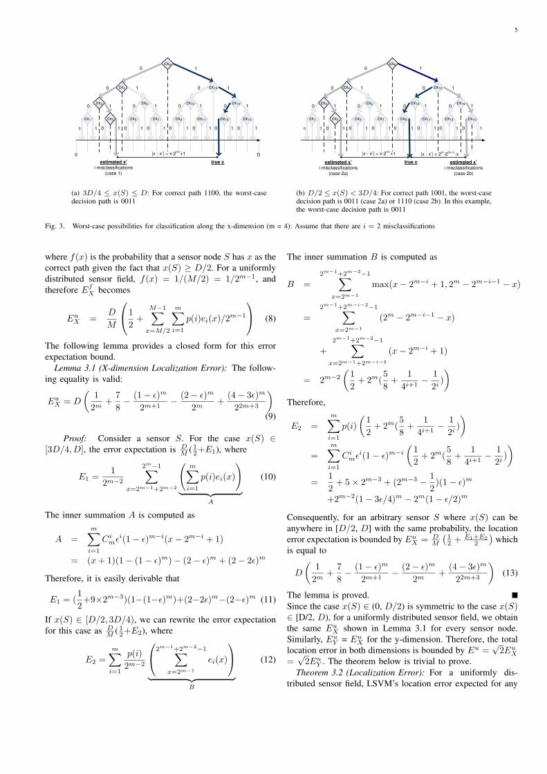
Consider a sensor S and localization along the x-dimension.Without loss of generality, suppose that x(S) ≥ D/2. Let x= x1x2...xm be the path on the decision tree that leads to thecorrect interval containing S, and x′ = x′1x

′2...x

′m the decision

path taken under the x-dimension localization algorithm. Sincewe estimate the x-coordinate of a sensor as the middle positionin the estimated interval, the x-dimension location error is atmost eX(x) = | x′−x | ×D/M + D/(2M) = D/M (1/2+ |x′ − x |).

Figure 3(a) illustrates a case where the correct path x =1100 and the decision path x′ = 0011 for are sensor S withtrue x(S) ∈ (12D/16, 13D/16]. There are 2 misclassificationsin the decision path: the decision S /∈ cx8 (i.e., x(S) < D/2)and the decision S /∈ cx4 (i.e., x(S) < D/4). These decisionsare wrong because x(S) > 12D/16 > D/2 > D/4. DecisionsS ∈ cx2 (i.e., x(S) ≥ D/8) and S ∈ cx3 (i.e., x(S) ≥ 3D/16)are correct.

In general, let i > 0 be the number of misclassificationsand p(i) the probability of their occurrence. Let ε be theworst error probability of SVM classification over all classescx1, cx2, ..., cxM−1, cy1, cy2, ..., cyM−1. Since there are mindependent classification steps in the localization algorithm,p(i) = Ci

mεi(1−ε)m−i. We will analyze the worst case whereei(x) = |x′ − x| is maximized. There are two cases:

1) If x(S) ∈ [3D/4, D] (i.e., x1 = x2 = 1): The worstcase occurs when all the first i classifications give wrongresults and the remaining classifications correct. That is,x′ = 0i1m−i, and therefore ei(x) = x − 0i1m−i = x− 2m−i + 1. (See Figure 3(a).)

2) If x(S) ∈ [D/2, 3D/4) (i.e., x1 = 1, x2 = 0): The worstcase must be one of the following scenarios: (see Figure3(b))

a) All the first i classifications give wrong results andthe remaining classifications correct: x′ = 0i1m−i

= 2m−i − 1 (e.g., the decision path 0011 in Figure3(b).)

b) The first classification is correct, the next i classi-fications wrong, and the remaining classificationscorrect: x′ = 1i+10m−i−1 = (2i+1 − 1)2m−i−1

= 2m − 2m−i−1 (e.g., the decision path 1110 inFigure 3(b).)

Therefore, ei(x) = max(x − 2m−i + 1, 2m − 2m−i−1

− x).Consequently, the x-dimension location error expected for

any node is bounded by

EfX =

M−1∑

x=M/2

eX(x)f(x) (6)

=D

M

1

2+

M−1∑

x=M/2

m∑

i=1

p(i)ei(x)f(x)

(7)

5

cx8

cx4

cx5cx3cx1 cx7

cx12

cx6cx2

cx13cx11cx9 cx15

cx14cx10

0

0

0 0 0 0

1

1

1

1

1 11

0

1 1 1 1 1 1 1 10 0 0 0 0 0 0 0

true xestimated x’

i misclassifications

(case 1)

|x - x’| = x-2m-i

+10 D

(a) 3D/4 ≤ x(S) ≤ D: For correct path 1100, the worst-casedecision path is 0011

cx8

cx4

cx5cx3cx1 cx7

cx12

cx6cx2

cx13cx11cx9 cx15

cx14cx10

0

0

0 0 0 0

1

1

1

1

1 11

0

1 1 1 1 1 1 1 10 0 0 0 0 0 0 0

true xestimated x’

i misclassifications

(case 2a)

|x - x’| = x-2m-i

+1 |x - x’| = 2m-2

m-i-1-x

estimated x’

i misclassifications

(case 2b)

(b) D/2 ≤ x(S) < 3D/4: For correct path 1001, the worst-casedecision path is 0011 (case 2a) or 1110 (case 2b). In this example,the worst-case decision path is 0011

Fig. 3. Worst-case possibilities for classification along the x-dimension (m = 4): Assume that there are i = 2 misclassifications

where f(x) is the probability that a sensor node S has x as thecorrect path given the fact that x(S) ≥ D/2. For a uniformlydistributed sensor field, f(x) = 1/(M/2) = 1/2m−1, andtherefore Ef

X becomes

EuX =

D

M

1

2+

M−1∑

x=M/2

m∑

i=1

p(i)ei(x)/2m−1

(8)

The following lemma provides a closed form for this errorexpectation bound.

Lemma 3.1 (X-dimension Localization Error): The follow-ing equality is valid:

EuX = D

(1

2m+

78− (1− ε)m

2m+1− (2− ε)m

2m+

(4− 3ε)m

22m+3

)

(9)

Proof: Consider a sensor S. For the case x(S) ∈[3D/4, D], the error expectation is D

M ( 12+E1), where

E1 =1

2m−2

2m−1∑

x=2m−1+2m−2

(m∑

i=1

p(i)ei(x)

)

︸ ︷︷ ︸A

(10)

The inner summation A is computed as

A =m∑

i=1

Cimεi(1− ε)m−i(x− 2m−i + 1)

= (x + 1)(1− (1− ε)m)− (2− ε)m + (2− 2ε)m

Therefore, it is easily derivable that

E1 = (12+9×2m−3)(1−(1−ε)m)+(2−2ε)m−(2−ε)m (11)

If x(S) ∈ [D/2, 3D/4), we can rewrite the error expectationfor this case as D

M ( 12+E2), where

E2 =m∑

i=1

p(i)2m−2

2m−1+2m−2−1∑

x=2m−1

ei(x)

︸ ︷︷ ︸B

(12)

The inner summation B is computed as

B =2m−1+2m−2−1∑

x=2m−1

max(x− 2m−i + 1, 2m − 2m−i−1 − x)

=2m−1+2m−i−2−1∑

x=2m−1

(2m − 2m−i−1 − x)

+2m−1+2m−2−1∑

x=2m−1+2m−i−2

(x− 2m−i + 1)

= 2m−2

(12

+ 2m(58

+1

4i+1− 1

2i))

Therefore,

E2 =m∑

i=1

p(i)(

12

+ 2m(58

+1

4i+1− 1

2i))

=m∑

i=1

Cimεi(1− ε)m−i

(12

+ 2m(58

+1

4i+1− 1

2i))

=12

+ 5× 2m−3 + (2m−3 − 12)(1− ε)m

+2m−2(1− 3ε/4)m − 2m(1− ε/2)m

Consequently, for an arbitrary sensor S where x(S) can beanywhere in [D/2, D] with the same probability, the locationerror expectation is bounded by Eu

X = DM

(12 + E1+E2

2

)which

is equal to

D

(1

2m+

78− (1− ε)m

2m+1− (2− ε)m

2m+

(4− 3ε)m

22m+3

)(13)

The lemma is proved.Since the case x(S) ∈ (0, D/2) is symmetric to the case x(S)∈ [D/2, D), for a uniformly distributed sensor field, we obtainthe same Eu

X shown in Lemma 3.1 for every sensor node.Similarly, Eu

Y = EuX for the y-dimension. Therefore, the total

location error in both dimensions is bounded by Eu =√

2EuX

=√

2EuY . The theorem below is trivial to prove.

Theorem 3.2 (Localization Error): For a uniformly dis-tributed sensor field, LSVM’s location error expected for any

6

0 20 40 60 80 1000

20

40

60

80

100

120

140

Parameter m

Bou

nd o

n ex

pect

atio

n of

wor

st−

case

loca

tion

erro

r

epsilon 0.01epsilon 0.05epsilon 0.1epsilon 0.2epsilon 0.3epsilon 0.4epsilon 0.5

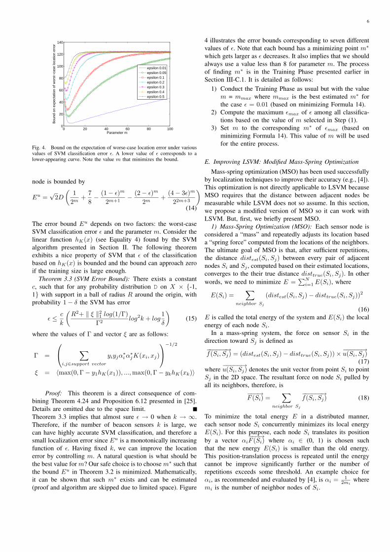
Fig. 4. Bound on the expectation of worse-case location error under variousvalues of SVM classification error ε. A lower value of ε corresponds to alower-appearing curve. Note the value m that minimizes the bound.

node is bounded by

Eu =√

2D

(1

2m+

78− (1− ε)m

2m+1− (2− ε)m

2m+

(4− 3ε)m

22m+3

)

(14)

The error bound Eu depends on two factors: the worst-caseSVM classification error ε and the parameter m. Consider thelinear function hK(x) (see Equality 4) found by the SVMalgorithm presented in Section II. The following theoremexhibits a nice property of SVM that ε of the classificationbased on hK(x) is bounded and the bound can approach zeroif the training size is large enough.

Theorem 3.3 (SVM Error Bound): There exists a constantc, such that for any probability distribution D on X × {-1,1} with support in a ball of radius R around the origin, withprobability 1− δ the SVM has error

ε ≤ c

k

(R2+ ‖ ξ ‖21 log(1/Γ)

Γ2log2k + log

1δ

)(15)

where the values of Γ and vector ξ are as follows:

Γ =

∑

i,j∈support vector

yiyjα∗i α∗jK(xi, xj)

−1/2

ξ = 〈max(0, Γ− y1hK(x1)), ..., max(0,Γ− ykhK(xk)〉

Proof: This theorem is a direct consequence of com-bining Theorem 4.24 and Proposition 6.12 presented in [25].Details are omitted due to the space limit.Theorem 3.3 implies that almost sure ε → 0 when k → ∞.Therefore, if the number of beacon sensors k is large, wecan have highly accurate SVM classification, and therefore asmall localization error since Eu is a monotonically increasingfunction of ε. Having fixed k, we can improve the locationerror by controlling m. A natural question is what should bethe best value for m? Our safe choice is to choose m∗ such thatthe bound Eu in Theorem 3.2 is minimized. Mathematically,it can be shown that such m∗ exists and can be estimated(proof and algorithm are skipped due to limited space). Figure

4 illustrates the error bounds corresponding to seven differentvalues of ε. Note that each bound has a minimizing point m∗

which gets larger as ε decreases. It also implies that we shouldalways use a value less than 8 for parameter m. The processof finding m∗ is in the Training Phase presented earlier inSection III-C.1. It is detailed as follows:

1) Conduct the Training Phase as usual but with the valuem = mmax where mmax is the best estimated m∗ forthe case ε = 0.01 (based on minimizing Formula 14).

2) Compute the maximum εmax of ε among all classifica-tions based on the value of m selected in Step (1).

3) Set m to the corresponding m∗ of εmax (based onminimizing Formula 14). This value of m will be usedfor the entire process.

E. Improving LSVM: Modified Mass-Spring Optimization

Mass-spring optimization (MSO) has been used successfullyby localization techniques to improve their accuracy (e.g., [4]).This optimization is not directly applicable to LSVM becauseMSO requires that the distance between adjacent nodes bemeasurable while LSVM does not so assume. In this section,we propose a modified version of MSO so it can work withLSVM. But, first, we briefly present MSO.

1) Mass-Spring Optimization (MSO): Each sensor node isconsidered a “mass” and repeatedly adjusts its location baseda “spring force” computed from the locations of the neighbors.The ultimate goal of MSO is that, after sufficient repetitions,the distance distest(Si, Sj) between every pair of adjacentnodes Si and Sj , computed based on their estimated locations,converges to the their true distance disttrue(Si, Sj). In otherwords, we need to minimize E =

∑Ni=1 E(Si), where

E(Si) =∑

neighbor Sj

(distest(Si, Sj)− disttrue(Si, Sj))2

(16)E is called the total energy of the system and E(Si) the localenergy of each node Si.

In a mass-spring system, the force on sensor Si in thedirection toward Sj is defined as−−−−−−→f(Si, Sj) = (distest(Si, Sj)− disttrue(Si, Sj))×−−−−−→u(Si, Sj)

(17)where

−−−−−→u(Si, Sj) denotes the unit vector from point Si to point

Sj in the 2D space. The resultant force on node Si pulled byall its neighbors, therefore, is

−−−→F (Si) =

∑

neighbor Sj

−−−−−−→f(Si, Sj) (18)

To minimize the total energy E in a distributed manner,each sensor node Si concurrently minimizes its local energyE(Si). For this purpose, each node Si translates its positionby a vector αi

−−−→F (Si) where αi ∈ (0, 1) is chosen such

that the new energy E(Si) is smaller than the old energy.This position-translation process is repeated until the energycannot be improve significantly further or the number ofrepetitions exceeds some threshold. An example choice forαi, as recommended and evaluated by [4], is αi = 1

2miwhere

mi is the number of neighbor nodes of Si.

7

TABLE INETWORK CONNECTIVITY SUMMARY

Radius Min degree Max degree Avg degree Netw. Diameterr=7m 2 27 14 25 (hops)r=10m 8 48 28 16 (hops)

2) Modified Mass-Spring Optimization (MMSO): SinceLSVM assumes no knowledge on the true distancedisttrue(Si, Sj), we use the communication range r of eachsensor in lieu of disttrue(Si, Sj). The energy of a sensor Si

is now defined as

E(Si) =∑

neighbor Sj

(distest(Si, Sj)− r)2 (19)

The force on Si pulled by Sj is redefined as

−−−−−−→f(Si, Sj) = (distest(Si, Sj)− r)×−−−−−→u(Si, Sj) (20)

Since we do not know the true distance, we only want to fixthose adjacent sensors whose estimated distance exceeds r.We therefore redefine the resultant force as follows:

−−−→F (Si) =

∑

neighbor Sj : distest(Si,Sj) > r

−−−−−−→f(Si, Sj) (21)

The MMSO algorithm conducted at node Si is summarizedbelow (for the case of stopping when the number of transla-tions exceeds some threshold):

Algorithm 3.2 (Modified Mass-Spring Optimization):Improve the location estimation of sensor Si:

1) Let thresholdcount be the system-defined maximalnumber of iterations

2) Let (xnew(Si), ynew(Si)) be the location of Si estimatedusing the LSVM localization algorithms presented inprevious sections (see Algorithm 3.1)

3) Compute mi the number of neighbors of Si, the currentenergy E(Si) according to Formula 19, and the currentforce

−−−→F (Si) according to Formula 21. Let fX and fY

be the x-dimension and y-dimension magnitudes of thisforce, respectively.

4) Compute possible new location

xnew(Si) = xcurrent(Si) +fX

2mi

ynew(Si) = ycurrent(Si) +fY

2mi

5) Compute possible new energy Enew(Si) according toFormula 19 using the new location (xnew(Si), ynew(Si))

6) IF (E(Si) > Enew(Si)), update the current position

xcurrent(Si) = xnew(Si)ycurrent(Si) = ynew(Si)

7) IF (number of iterations exceeds thresholdcount) QUIT8) ELSE GOTO Step 3

TABLE IISVM CLASSIFICATION ACCURACY (MIN/AVG) PER CLASS FOR DIFFERENT

RANGES AND BEACON POPULATIONS

Axis 5% 10% 15% 20% 25%Range 10m x .89/.95 .92/.96 .95/.98 .95/.98 .96/.98

y .90/.96 .91/.97 .93/.98 .95/.98 .95/.98Range 7m x .91/.96 .92/.97 .94/.98 .95/.98 .95/.98

y .90/.96 .91/.97 .93/.98 .95/.98 .96/.98

TABLE IIIAVERAGE NUMBER OF SUPPORT VECTORS PER CLASS FOR DIFFERENT

RANGES AND BEACON POPULATIONS

Axis 5% 10% 15% 20% 25%Range 10m x 14.29 20.48 22.55 33.31 42.62

y 13.85 23.16 27.08 25.30 29.08Range 7m x 12.40 17.57 23.44 34.70 29.55

y 16.55 24.92 30.96 27.34 26.37

IV. SIMULATION STUDY

We conducted a simulation study on a network of 1000sensors located in a 100m × 100m 2-D area. We assumeduniform random distribution for the sensor locations and theselection of the beacon sensors. We considered two levelsof network density (7m and 10m communication ranges),summarized in Table I. We also considered five differentbeacon populations: 5% of the network size (k = 50 beacons),10% (k = 100 beacons), 15% (k = 150 beacons), 20% (k =200 beacons), and 25% (k = 250 beacons). The computationalcost of LSVM is theoretically analyzed in Section III-C. Thecommunication cost is mainly due to k broadcasts where k isthe number of beacons. We, therefore, focused more on thelocalization accuracy.

We used the algorithms in the libsvm [24] software forSVM classification. The γ parameter in Equation 5 and Cparameter in Inequality 3 were automatically determined bythe mechanisms of libsvm. We set m = 7 (i.e., M = 128) bydefault, the rationale for which will be explained in SectionIV-A.

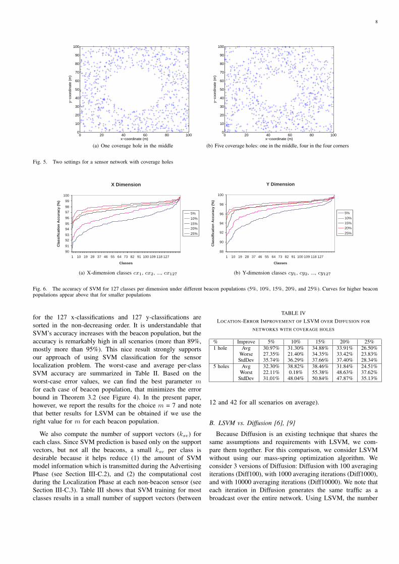
Many networking protocols such as routing and localizationsuffer from the existence of coverage holes or obstacles in thesensor field. We considered three sensor networks: a networkwith no coverage hole and two following networks with holeexistence: (1) a network with one hole centered at position(50,50) of radius 25m (Figure 5(a)), and (2) a network with5 holes, one at (50,50) of radius 100

6 m and the other four ofradius 100

12 m at the four corners of the field (Figure 5(b)).In the following sections, we discuss the results (in present

tense for ease of presentation) of the following studies: qualityand efficiency of SVM classification, comparisons betweenLSVM and two existing techniques (Diffusion [6], [9] andAFL [4]), and, finally, the performance of LSVM under theeffects of beacon population, network density, the borderproblem, and coverage holes.

A. Quality and efficiency of SVM classification

As analyzed in Section III-D, the SVM classification error isan important factor to the accuracy of LSVM. The quality ofSVM is demonstrated in Figure 6, in which the accuracies

8

0 20 40 60 80 1000

10

20

30

40

50

60

70

80

90

100

x−coordinate (m)

y−co

ordi

nate

(m

)

(a) One coverage hole in the middle

0 20 40 60 80 1000

10

20

30

40

50

60

70

80

90

100

x−coordinate (m)

y−co

ordi

nate

(m

)

(b) Five coverage holes: one in the middle, four in the four corners

Fig. 5. Two settings for a sensor network with coverage holes

X Dimension

90

91

92

93

94

95

96

97

98

99

100

1 10 19 28 37 46 55 64 73 82 91 100 109 118 127

Classes

Cla

ssif

icat

ion

Acc

ura

cy (

%)

5%

10%

15% 20%

25%

(a) X-dimension classes cx1, cx2, ..., cx127

Y Dimension

88

90

92

94

96

98

100

1 10 19 28 37 46 55 64 73 82 91 100 109 118 127

Classes

Cla

ssif

icat

ion

Acc

ura

cy (

%)

5%

10% 15% 20%

25%

(b) Y-dimension classes cy1, cy2, ..., cy127

Fig. 6. The accuracy of SVM for 127 classes per dimension under different beacon populations (5%, 10%, 15%, 20%, and 25%). Curves for higher beaconpopulations appear above that for smaller populations

for the 127 x-classifications and 127 y-classifications aresorted in the non-decreasing order. It is understandable thatSVM’s accuracy increases with the beacon population, but theaccuracy is remarkably high in all scenarios (more than 89%,mostly more than 95%). This nice result strongly supportsour approach of using SVM classification for the sensorlocalization problem. The worst-case and average per-classSVM accuracy are summarized in Table II. Based on theworst-case error values, we can find the best parameter mfor each case of beacon population, that minimizes the errorbound in Theorem 3.2 (see Figure 4). In the present paper,however, we report the results for the choice m = 7 and notethat better results for LSVM can be obtained if we use theright value for m for each beacon population.

We also compute the number of support vectors (ksv) foreach class. Since SVM prediction is based only on the supportvectors, but not all the beacons, a small ksv per class isdesirable because it helps reduce (1) the amount of SVMmodel information which is transmitted during the AdvertisingPhase (see Section III-C.2), and (2) the computational costduring the Localization Phase at each non-beacon sensor (seeSection III-C.3). Table III shows that SVM training for mostclasses results in a small number of support vectors (between

TABLE IVLOCATION-ERROR IMPROVEMENT OF LSVM OVER DIFFUSION FOR

NETWORKS WITH COVERAGE HOLES

% Improve 5% 10% 15% 20% 25%1 hole Avg 30.97% 31.30% 34.88% 33.91% 26.50%

Worse 27.35% 21.40% 34.35% 33.42% 23.83%StdDev 35.74% 36.29% 37.66% 37.40% 28.34%

5 holes Avg 32.30% 38.82% 38.46% 31.84% 24.51%Worst 22.11% 0.18% 55.38% 48.63% 37.62%

StdDev 31.01% 48.04% 50.84% 47.87% 35.13%

12 and 42 for all scenarios on average).

B. LSVM vs. Diffusion [6], [9]

Because Diffusion is an existing technique that shares thesame assumptions and requirements with LSVM, we com-pare them together. For this comparison, we consider LSVMwithout using our mass-spring optimization algorithm. Weconsider 3 versions of Diffusion: Diffusion with 100 averagingiterations (Diff100), with 1000 averaging iterations (Diff1000),and with 10000 averaging iterations (Diff10000). We note thateach iteration in Diffusion generates the same traffic as abroadcast over the entire network. Using LSVM, the number

9

LSVM vs. Diffusion

0

1

2

3

4

5

6

7

8

9

10

Diff100 Diff1000 Diff10000 Lsvm

Techniques in comparison

Avg

. Lo

cati

on

Err

or

(m)

5% 10% 15% 20% 25%

(a) Average location error

LSVM vs. Diffusion

0

5

10

15

20

25

30

35

1 2 3 4

Techniques in comparison

Max

. Lo

cati

on

Err

or

(m)

5% 10% 15% 20% 25%

(b) Max location error

LSVM vs. Diffusion

0

1

2

3

4

5

6

7

Diff100 Diff1000 Diff10000 Lsvm

Techniques in comparison

Lo

cati

on

Err

or

Std

. Dev

. (m

)

5% 10% 15% 20% 25%

(c) Standard deviation

Fig. 7. LSVM vs. Diffusion (range 10m): Statistics on location error of each technique under different beacon populations

of broadcasts incurred is the number of beacon sensors, whichis much smaller than in the case of Diffusion.

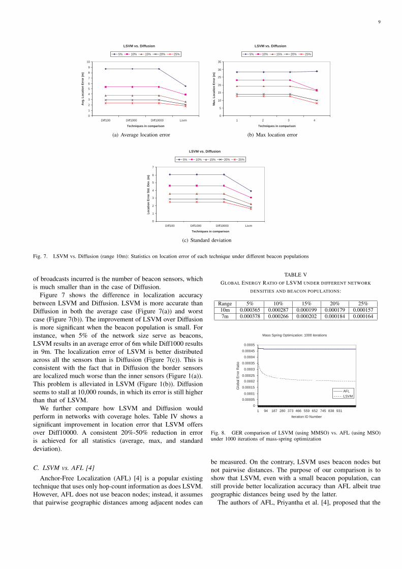
Figure 7 shows the difference in localization accuracybetween LSVM and Diffusion. LSVM is more accurate thanDiffusion in both the average case (Figure 7(a)) and worstcase (Figure 7(b)). The improvement of LSVM over Diffusionis more significant when the beacon population is small. Forinstance, when 5% of the network size serve as beacons,LSVM results in an average error of 6m while Diff1000 resultsin 9m. The localization error of LSVM is better distributedacross all the sensors than is Diffusion (Figure 7(c)). This isconsistent with the fact that in Diffusion the border sensorsare localized much worse than the inner sensors (Figure 1(a)).This problem is alleviated in LSVM (Figure 1(b)). Diffusionseems to stall at 10,000 rounds, in which its error is still higherthan that of LSVM.

We further compare how LSVM and Diffusion wouldperform in networks with coverage holes. Table IV shows asignificant improvement in location error that LSVM offersover Diff10000. A consistent 20%-50% reduction in erroris achieved for all statistics (average, max, and standarddeviation).

C. LSVM vs. AFL [4]

Anchor-Free Localization (AFL) [4] is a popular existingtechnique that uses only hop-count information as does LSVM.However, AFL does not use beacon nodes; instead, it assumesthat pairwise geographic distances among adjacent nodes can

TABLE VGLOBAL ENERGY RATIO OF LSVM UNDER DIFFERENT NETWORK

DENSITIES AND BEACON POPULATIONS:

Range 5% 10% 15% 20% 25%10m 0.000365 0.000287 0.000199 0.000179 0.0001577m 0.000378 0.000266 0.000202 0.000184 0.000164

Mass Spring Optimization: 1000 iterations

0

0.00005

0.0001

0.00015

0.0002

0.00025

0.0003

0.00035

0.0004

0.00045

0.0005

1 94 187 280 373 466 559 652 745 838 931

Iteration ID Number

Glo

bal E

rror

Rat

io

AFL

LSVM

Fig. 8. GER comparison of LSVM (using MMSO) vs. AFL (using MSO)under 1000 iterations of mass-spring optimization

be measured. On the contrary, LSVM uses beacon nodes butnot pairwise distances. The purpose of our comparison is toshow that LSVM, even with a small beacon population, canstill provide better localization accuracy than AFL albeit truegeographic distances being used by the latter.

The authors of AFL, Priyantha et al. [4], proposed that the

10

Global Energy Ratio (GER) be used to assess the localizationaccuracy. Therefore, we use GER to compare AFL and LSVM:

GER =

√∑i<j

(distest(Si,Sj)−disttrue(Si,Sj)

disttrue(Si,Sj)

)2

N(N − 1)/2(22)

GER captures the distance error; that is, to how close theestimated geographic distance distest(Si, Sj) between a pairof sensors is to their true geographic distance disttrue(Si, Sj).GER also captures the structural error of the graph inducedby the estimated locations.

As reported in [4], the GER of AFL varies between 0.0001and 0.0012 depending on the error of edge-length measure-ment and increases with the network density, but only slightlywhen average nodal degree exceeds 9. Table V provides theGER results of LSVM, which shows that the GER of LSVMis in the top accuracy range of AFL.

AFL must rely on an iterative process of mass-springoptimization (MSO) to refine its location estimation. LSVMhas an option of using the modified mass-spring optimiza-tion (MMSO) algorithm (i.e., Algorithm 3.2) to refine itslocalization. Figure 8 plots the GER values for AFL and50-beacon LSVM during the optimization process of 1000iterations. Although we use the true geographic distances forthe measurement of pairwise distances in AFL, it remainsfar less accurate than LSVM even though only 50 beaconnodes are used with LSVM. Additionally, LSVM improvessignificantly faster than AFL as we continue the MSO process.AFL does not seem to ever approach the accuracy of LSVMeven when LSVM does not use MMSO. This study suggeststhat (1) our proposed MMSO algorithm is effective, and(2) when beacon nodes are available, LSVM is much moreaccurate and faster to converge than AFL. AFL has beeneffective to initialize the sensor locations in small networks[21]. For large-scale networks, however, LSVM is a moresuitable choice.

D. LSVM: Effect of network density and beacon population,the coverage-hole problem, and the border problem

In the remainder of this section, we evaluate LSVM underthe effect of network density and beacon population, thecoverage-hole problem, and the border problem. We alsoinclude the results for Diff1000 (Diffusion with 1000 loops)as a reference. The results are presented below.

1) Network density: We investigate LSVM under two levelsof network density. In one network, the communication rangeof each sensor is set to r = 7m; in the other, set to r = 10m.The connectivity summary of these two networks is shownin Table I. The latter network is two times more connectedthan the former (i.e., doubling the node degree and edges).Figure 9 suggests that reducing the network density onlyslightly increase location error of LSVM. In contrary, it isobserved that its counterpart Diffusion is more accurate inless network density. In comparison, LSVM in a less densenetwork (i.e., Lsvm-r7) still performs no worse than the bestof its counterpart Diffusion (i.e., Diff1000-r7) in all statistics:

average error (Figure 9(a)), worst-case error (Figure 9(b)), anderror distribution (Figure 9(c)). In terms of standard deviation,Lsvm-r7 is remarkably better than Diff1000-r7.

2) Number of beacon sensors: Figure 9 also illustrates anobvious feature of LSVM that the localization accuracy getsbetter as more beacon sensors are used. Using only 5% (k =50), we can locate a sensor within a mean error of 5.5m ina 10,000m2 square field. When k = 100 beacons, the erroris reduced to 3.6m. The reduction is less significant whenwe continue to increase k. This study suggests that for costeffectiveness between 5% and 15% of the network size beused as beacon sensors.

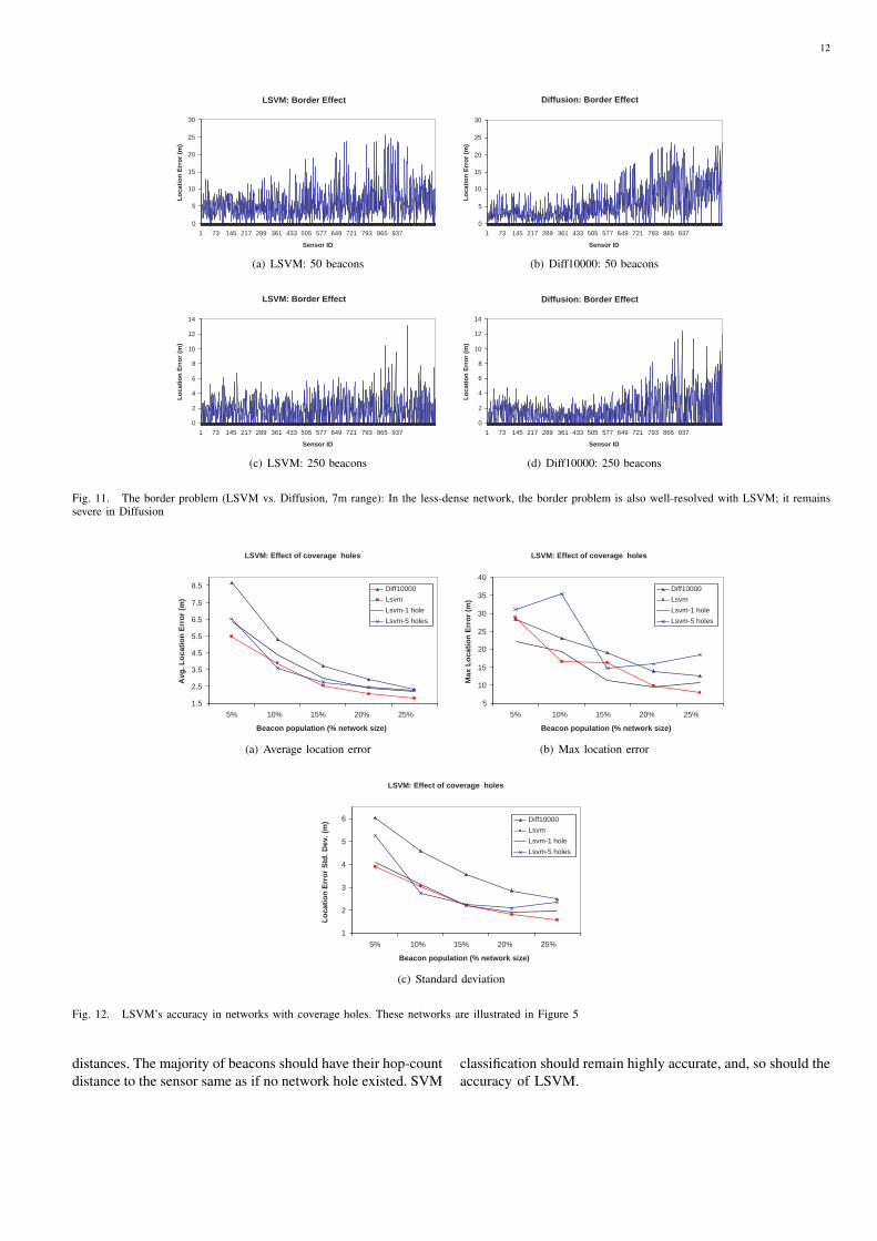
3) The border problem: The border problem, where sensorsclose to the edge of the sensor field are poorly positionedcompared to those deep inside the field, is a challenge formany techniques. We investigate this problem for two typesof network (communication range 7m and 10m) and two sizesof beacon population (5% and 25% network size). Figures 10and 11 show the location error for every sensor node, sortedin the increasing order of sensor distance to the field’s origin,for two different network densities (r = 10m and r = 7m). Inother words, those sensors closer to the origin appear beforethose closer to the edge. In all scenarios, Diff10000 suffersfrom the border problem severely (i.e., significantly largererror for border-close sensors). On the other hand, LSVMaddresses this problem much better, as illustrated in Figures10(a), 10(c), 11(a), 11(c). The differences between the locationerrors of sensors closer to the edge and that of sensors insideare much less significant. This property can be explained. InDiffusion, the localization of a sensor is based on its neighbors,whose estimated location in turn depends on other neighbors.Sensors near the border have less neighbor information thanthose inside the field. Therefore, the former’s location estimateshould be less accurate. LSVM does not suffer from thisproblem because the localization of a sensor is only basedon the beacon nodes directly, which is independent of othersensors. Therefore, whether a sensor is near the border or thefield’s center should not have a big impact on its locationestimation.

4) Existence of network holes: We consider the two net-works demonstrated in Figure 5: a network with 1 hole (Figure5(a)) and a network with 5 holes (Figure 5(b)). Figure 12shows the localization error of LSVM in these networks. Wealso use the error of Diff10000 in the hole-less network as thereference line. It is understandable that LSVM may be lessaccurate in the networks with holes; however, the existence ofcoverage holes does not seem to have an impact on LSVM.The reduction in error, if there exists, is very minor. Moreover,LSVM in the networks with holes provides even much betteraccuracy and error deviation than Diff10000 in the hole-lessnetworks. For example, with 50 beacons, while Diff10000 inthe case of no coverage hole has an average error of 8.5mand standard deviation of 6m, the average error and standarddeviation of LSVM in the case of networks with holes areless than 6.5m and 5m, respectively. Therefore, LSVM canhandle not only the border problem, but also the coverage-holeproblem. Similar to the border issue, the coverage-hole issuecan be explained as well. Although there are network holes, the

11

LSVM: Effect of network density

1.5

2.5

3.5

4.5

5.5

6.5

7.5

8.5

5% 10% 15% 20% 25%

Beacon population (% network size)

Avg

. Lo

cati

on

Err

or

(m)

Lsvm-r10

Lsvm-r7

Diff10000-r10

Diff10000-r7

(a) Average location error

LSVM: Effect of network density

5

10

15

20

25

30

5% 10% 15% 20% 25%

Beacon population (% network size)

Max

. Lo

cati

on

Err

or

(m)

Lsvm-r10

Lsvm-r7

Diff10000-r10

Diff10000-r7

(b) Max location error

LSVM: Effect of network density

1.5

2

2.5

3

3.5

4

4.5

5

5.5

6

6.5

5% 10% 15% 20% 25%

Beacon population (% network size)

Lo

cati

on

Err

or

Std

. Dev

. (m

) Lsvm-r10

Lsvm-r7

Diff10000-r10

Diff10000-r7

(c) Standard deviation

Fig. 9. LSVM under the effect of network density (r = 7m and r = 10m): Statistics on location error per each beacon population

LSVM: Border Effect

0

5

10

15

20

25

30

1 73 145 217 289 361 433 505 577 649 721 793 865 937

Sensor ID

Lo

cati

on

Err

or

(m)

(a) LSVM: 50 beacons

Diffusion: Border Effect

0

5

10

15

20

25

30

1 73 145 217 289 361 433 505 577 649 721 793 865 937

Sensor ID

Lo

cati

on

Err

or

(m)

(b) Diff10000: 50 beacons

LSVM: Border Effect

0

2

4

6

8

10

12

14

1 73 145 217 289 361 433 505 577 649 721 793 865 937

Sensor ID

Lo

cati

on

Err

or

(m)

(c) LSVM: 250 beacons

Diffusion: Border Effect

0

2

4

6

8

10

12

14

1 73 145 217 289 361 433 505 577 649 721 793 865 937

Sensor ID

Lo

cati

on

Err

or

(m)

(d) Diff10000: 250 beacons

Fig. 10. The border problem (LSVM vs. Diffusion, 10m range): Location error for every sensor, sorted in the order of nodes close to the origin of the fieldfirst and nodes close to the edge of the field last. The border problem is resolved well with LSVM; it is severe in Diffusion because the error is significantlyincreased toward the edge

hop-count distances between a sensor and only a small number of beacons become less representative of their true geographic

12

LSVM: Border Effect

0

5

10

15

20

25

30

1 73 145 217 289 361 433 505 577 649 721 793 865 937

Sensor ID

Lo

cati

on

Err

or

(m)

(a) LSVM: 50 beacons

Diffusion: Border Effect

0

5

10

15

20

25

30

1 73 145 217 289 361 433 505 577 649 721 793 865 937

Sensor ID

Lo

cati

on

Err

or

(m)

(b) Diff10000: 50 beacons

LSVM: Border Effect

0

2

4

6

8

10

12

14

1 73 145 217 289 361 433 505 577 649 721 793 865 937

Sensor ID

Lo

cati

on

Err

or

(m)

(c) LSVM: 250 beacons

Diffusion: Border Effect

0

2

4

6

8

10

12

14

1 73 145 217 289 361 433 505 577 649 721 793 865 937

Sensor ID

Lo

cati

on

Err

or

(m)

(d) Diff10000: 250 beacons

Fig. 11. The border problem (LSVM vs. Diffusion, 7m range): In the less-dense network, the border problem is also well-resolved with LSVM; it remainssevere in Diffusion

LSVM: Effect of coverage holes

1.5

2.5

3.5

4.5

5.5

6.5

7.5

8.5

5% 10% 15% 20% 25%

Beacon population (% network size)

Avg

. Lo

cati

on

Err

or

(m)

Diff10000

Lsvm

Lsvm-1 hole

Lsvm-5 holes

(a) Average location error

LSVM: Effect of coverage holes

5

10

15

20

25

30

35

40

5% 10% 15% 20% 25%

Beacon population (% network size)

Max

Lo

cati

on

Err

or

(m)

Diff10000

Lsvm

Lsvm-1 hole

Lsvm-5 holes

(b) Max location error

LSVM: Effect of coverage holes

1

2

3

4

5

6

5% 10% 15% 20% 25%

Beacon population (% network size)

Lo

cati

on

Err

or

Std

. Dev

. (m

) Diff10000

Lsvm

Lsvm-1 hole

Lsvm-5 holes

(c) Standard deviation

Fig. 12. LSVM’s accuracy in networks with coverage holes. These networks are illustrated in Figure 5

distances. The majority of beacons should have their hop-countdistance to the sensor same as if no network hole existed. SVM

classification should remain highly accurate, and, so should theaccuracy of LSVM.

13

V. CONCLUSION

We have presented LSVM – a distributed localization tech-nique for sensor networks based on the concept of SupportVector Machines. LSVM assumes the existence of a number ofbeacons and uses them as training data to the learning process.

Only mere connectivity information is used in LSVM,making it suitable for networks that do not require pairwisedistance measurement and specialized (and/or mobile) assist-ing devices. LSVM yet provides encouraging results. Our sim-ulation study have shown that LSVM outperforms Diffusion,a popular approach that shares the same assumptions withLSVM. With a small beacon population, LSVM has beenshown to also be faster converging and more accurate thanAFL, a popular technique that requires pairwise distance mea-surement. LSVM alleviates the border problem and remainseffective in networks with coverage holes/obstacles, whichmany other techniques currently suffer from. The communi-cation and processing overheads are kept small. We have alsoevaluated LSVM analytically and provided theoretical boundson its localization accuracy.

In network scenarios that can afford ranging and assistingdevices to measure geographic pair-wise distances, becauseof its simplicity and fast convergence, LSVM can be used toprovide good starting locations for the sensors. The locationestimation of LSVM can, optionally, be refined using ourmodified mass-spring optimization algorithm.

The next step in our research is to evaluate LSVM in othernetwork scenarios, including various distribution models forthe sensor locations, coverage holes, and network density. Wewould also like to implement LSVM as a real prototype systemand investigate its applicability in fading environments as wellas networks of moving sensors with different communicationranges.

REFERENCES

[1] L. Doherty, L. E. Ghaoui, and K. S. J. Pister, “Convex positionestimation in wireless sensor networks,” in IEEE Infocom, April 2001.

[2] Shang, Juml, Zhang, and Fromherz, “Localization from mere connec-tivity,” in ACM Mobihoc, 2003.

[3] C. Savarese, J. Rabaey, and J. Beutel, “Locationing in distributed ad-hoc wireless sensor networks,” in IEEE International Conference onAcoustics, Speech, and Signal Processing, Salt Lake city, UT, 2001.

[4] N. B. Priyantha, H. Balakrishnan, E. Demaine, and S. Teller, “Anchor-free distributed localization in sensor networks,” in ACM Sensys, 2003.

[5] S. Capkun, M. Hamdi, and J.-P. Hubauz, “Gps-free positioning inmobile ad hoc networks,” in Hawai International Conference on SystemSciences, 2001.

[6] L. Meertens and S. Fitzpatrick, “The distributed construction of a globalcoordinate system in a network of static computational nodes from inter-node didstances,” Kestrel Institute, Tech. Rep., 2004.

[7] D. Moore, J. Leonard, D. Rus, and S. Teller, “Robust distributed networklocalization with noisy range measurements,” in ACM Sensys, Baltimore,MA, November 2004.

[8] D. Niculescu and B. Nath, “Ad hoc positioning system (aps),” in IEEEGlobecom, 2001.

[9] N. Bulusu, V. Bychkovskiy, D. Estrin, and J. Heidemann, “Scalable adhoc deployable rf-based localization,” in Grace Hopper Celebration ofWomen in Computing Conference, Vancouver, Canada, October 2002.

[10] A. Savvides, H. Park, and M. Srivastava, “The bits and flops of the n-hopmultilateration primitive for node localization problems,” in Workshopon Wireless Networks and Applications (in conjunction with Mobicom2002), Atlanta, GA, September 2002.

[11] A. Savvides, C.-C. Han, and M. B. Strivastava, “Dynamic fine-grainedlocalization in ad hoc networks of sensors,” in ACM InternationalConference on Mobile Computing and Networking (Mobicom), Rome,Italy, July 2001, pp. 166–179.

[12] S. Simic and S. S. Sastry, “Distributed localization in wireless ad hocnetworks,” University of California at Berkeley, Tech. Rep., 2002.

[13] C. Whitehouse, “The design of calamari: an ad hoc localization sys-tem for sensor networks,” Master’s thesis, University of California atBerkeley, 2002.

[14] D. Niculescu and B. Nath, “Ad hoc positioning system (aps) using aoa,”in IEEE Infocom, 2003.

[15] R. Nagpal, H. Shrobe, and J. Bachrach, “Organizing a global coordinatesystem from local information on an ad hoc sensor network,” inInternational Symposium on Information Processing in Sensor Networks,2003.

[16] T. He, C. Huang, B. Blum, J. Stankovic, and T. Abdelzaher, “Range-freelocalization schemes in large scale sensor networks,” in ACM Conferenceon Mobile Computing and Networking, 2003.

[17] N. B. Priyantha, “The cricket indoor location system,” Ph.D. dissertation,Massachussette Institute of Technology, 2005.

[18] Y. Kwon, K. Mechitov, S. Sundresh, W. Kim, and G. Agha, “Resilientlocalization for sensor networks in outdoor environments,” University ofIllinois at Urbana-Champaign, Tech. Rep., June 2004.

[19] N. Priyantha, A. Miu, H. Balakrishnan, and S. Teller, “The cricketcompass for context-aware mobile applications,” in ACM conference onmobile computing and networking (MOBICOM), 2001.

[20] R. Stoleru, J. A. Stankovic, and D. Luebke, “A high-accuracy, low-costlocalization system for wireless sensor networks,” in ACM Sensys, SanDiego, CA, November 2005.

[21] N. B. Priyantha, H. Balakrishnan, E. Demaine, and S. Teller, “Mobile-Assisted Localization in Wireless Sensor Networks,” in IEEE INFO-COM, Miami, FL, March 2005.

[22] X. Nguyen, M. Jordan, and B. Sinopoli, “A kernel-based learningapproach to ad hoc sensor network localization,” IEEE Transactionson Sensor Networks, vol. 1, pp. 134–152, 2005.

[23] V. N. Vapnik, Statistical Learning Theory. Wiley-Interscience, 1998.[24] C.-C. Chang and C.-J. Lin, LIBSVM – A library for Support

Vector Machines, National Taiwan University. [Online]. Available:http://www.csie.ntu.edu.tw/ cjlin/libsvm

[25] N. Cristianini and J. Shawe-Taylor, An introduction to Support VectorMachines and other kernel-based learning methods. CambridgeUniversity Press, 2003.

Duc A. Tran is an Assistant Professor at the Uni-versity of Dayton, where he conducts research in theareas of Computer Networks, Distributed Systems,and Multimedia Systems. His current work is fundedby the NSF and the Ohio Board of Regents. Dr. Tranhas served as a Vice Program Chair for IEEE AINA2007, journal guest-editor, TPC member for 12international conferences, and referee for numerousACM/IEEE international conferences and journals.His PhD degree in Computer Science was from theUniversity of Central Florida in May 2003, where

he also received the Distinguished Doctoral Research Award, IEEE-OrlandoOutstanding Graduate Student Award, and the Order of Pegasus Award.

Thinh Nguyen has been an Assistant Professor atOregon State University since 2004. He earned aB.S. from the University of Washington, and anM.S. and Ph.D. from U.C. Berkeley in 2000 and2003, respectively. During 2003-2004, he was a post-doctoral research associate at Lawrence LivermoreNational Laboratory. During 1996-1998, he was agraphics researcher at Intel’s Microcomputer Re-search Lab. He also spent 6 months at Microsoft,optimizing DirectX6 for Pentium III. Dr. Nguyen’scurrent research interests include networking, signal

processing, computer graphics, machine learning, data analysis and datamining.