Practical Impacts of Ambient Temperature A DECADE OF and ...

Localised economic impacts from high 1
temperature disruption days under climate change 2
Authors: 3
Tim Summers (1), Erik Mackie (2, 3), Risa Ueno (3, 5), Charles Simpson (3), J. Scott 4
Hosking (3, 4), Tudor Suciu (6), Andrew Coburn (1), Emily Shuckburgh (2, 6) 5
6
This paper is a non-peer reviewed preprint submitted to EarthArXiv. It has also been 7
submitted to the journal ‘Climate Resilience and Sustainability’. 8
Affiliations: 9
1. Centre for Risk Studies, Judge Business School, University of Cambridge 10
2. Cambridge Zero, University of Cambridge 11
3. British Antarctic Survey, NERC 12
4. The Alan Turing Institute 13
5. Department of Chemistry, University of Cambridge 14
6. Department of Computer Science & Technology, University of Cambridge 15
Emails: 16
Twitter: 25
@emilyshuckburgh, @Summertim, @ErikMackie, @scotthosking 26
Address for correspondence: 27
28
Dr T Summers, 29
Centre for Risk Studies, 30
Cambridge Judge Business School, 31
University of Cambridge, 32
Trumpington Street, 33
Cambridge 34
CB2 1AG, 35
UK 36
37

Data availability: Our analysis is based on data available via CEDA’s data analysis 38
environment JASMIN https://help.jasmin.ac.uk/article/189-get-started-with-jasmin . 39
40
41

Abstract 42
Most studies into the effects of climate change have headline results in the form of a global 43
change in mean temperature. More useful for businesses and governments however are 44
measures of the economic impact, either direct or indirect. We have addressed this by 45
examining how the frequency of exceeding a daily mean temperature threshold changes, 46
defined as “disruption days”, as it is often this exceedance which has the most dramatic 47
impacts on personal or economic behaviour. Our exceedance analysis tackles the resolution 48
of climate change both geographically and temporally, the latter specifically to address the 5-49
20 year time horizon which can be recognised in business planning. 50
We apply bias correction with quantile mapping to meteorological reanalysis data from 51
ECMWF ERA5 and output from CMIP5 climate model simulations. By determining the daily 52
frequency at which a mean temperature threshold is exceeded in this bias-corrected dataset, 53
we can compare predicted and historic frequencies to estimate the change in the number of 54
disruption days. Furthermore, by combining results from 18 different climate models, we can 55
estimate the likelihood of more extreme events, taking into account model variations. This is 56
useful for worst case scenario planning. 57
Taking the city of Chicago as an example, the expected frequency of years with 40 or more 58
disruption days above the 25ºC threshold rises by a factor of four for a time period centred 59
on 2040, compared with a period centred on 2000. Alternately, looking at the change in the 60
number of days at a given likelihood, an example is Shenzhen, where the number of 61
disruption days in a once-per-decade event exceeding the 25ºC or 30ºC threshold is 62
expected to rise by a factor of four. 63
Superimposing these results onto maps of, for instance, GDP sensitivity or production days 64
lost, will provide more accurate and targeted conclusions for future impacts of climate 65
change. This method of quantifying costs on business-relevant timescales will help 66
businesses and governments properly include risks associated with facilities, plan mitigating 67
actions and make accurate provisions. It can also, for example, inform their disclosure of 68
physical risks under the framework of the Task Force on Climate-related Financial 69
Disclosures. This approach is equally applicable to other weather-related, localised 70
phenomena likely to be impacted by climate change. 71
Keywords: 72
economic, disruption, climate, temperature, bias, correction, exceedance 73
Introduction 74
Human-induced climate change has resulted in over 1.0ºC of global warming to-date, when 75
compared with pre-industrial levels (IPCC 2018). The impacts of this warming trend on 76
human and natural systems are already being felt around the world, in part through an 77
increase in the likelihood of extreme weather events such as heatwaves. For example, the 78
recent Siberian heatwave (January - June 2020) has been shown to be at least 600 times 79
more likely as a result of human-induced climate change (Kew et al. 2020), while the 80
probability of the conditions occurring that led to the 2019/2020 Australian bushfires are 81

estimated to have increased by at least 30% since 1900, due to anthropogenic climate 82
change (van Oldenborgh et al. 2020). These risks will increase with future warming. 83
The acute impact of climate change on business and society can be directly observed 84
through changes to the tails of climatic distributions, as extreme events become more likely 85
or more severe. But they are much harder to infer from apparently small changes in central 86
statistics like the rise in the annual global average temperature. Extreme weather events can 87
have adverse financial impacts on businesses through damage to physical assets, disruption 88
or reduction in productivity of operations and supply chains, and impacts to market demand 89
for products and services (Handmer et al. 2012). 90
These risks are of growing concern for businesses, and many corporations are trying to 91
understand how present and future changes in extreme weather risk are likely to affect them. 92
Organisations are under pressure to take action to address environmental, social and 93
corporate governance (ESG) demands, and for strategic and competitive reasons, as well as 94
address regulatory requirements or other liabilities they may face. Mapping the geographical 95
overlap of extreme weather events and business systems is key to providing insight to global 96
corporates of the exposure of their entire value chains to physical climate change risk. 97
These needs are framed by the recommendations of the Task Force for Climate-related 98
Financial Disclosures (TCFD), which has been voluntarily adopted by more than 1,500 99
global organisations as of October 2020 (TCFD 2020). Investors are mobilising to pressure 100
companies to respond to the TCFD recommendations and disclose climate-related risks, 101
with the threat that they will be less inclined to invest in companies that fail to do so (Eccles, 102
2018). Companies that comply with the recommendations will have better strategies to adapt 103
to climate change and may be more able to harness any potential opportunities that climate 104
change presents. 105
The TCFD includes a recommendation to describe the impacts of acute (i.e. extreme) 106
weather events, causing physical risks on an organisation over three time horizons, typically 107
below 5 years, five to ten years and beyond ten years. Organisations’ energies are typically 108
more focused on short time-frames that they use to conduct operational, financial, strategic, 109
and capital planning (TCFD 2020). However, the currently available data and model 110
projections of future changes in extreme weather risk often do not suit the requirements of 111
businesses. Organisations are struggling to reconcile the long-term projections of the 112
consequences of a warmer planet in several decades' time with changes in the frequency, 113
severity, and geography of extreme weather events that are already having financial impacts 114
on their businesses. 115
Economic productivity is particularly sensitive to extreme heat and associated hazards, 116
which can affect large regions simultaneously to produce widespread impacts and economic 117
loss (Handmer et al. 2012). These impacts are variable across sectors, and particularly 118
affect those relying on labour-intensive activities such as agriculture, manufacturing, and 119
construction (Zuo et al. 2015, Simpson et al., 2021). Human output is impacted through time 120
loss resulting from the heat-induced health outcomes, or ‘absenteeism’, as well as 121
reductions in work productivity and capacity, termed ‘presenteeism’ (Xia et al. 2018). 122
Infrastructure, transportation, and energy systems are also vulnerable to extreme heat, and 123
physical damage or service outages can severely disrupt supply chain activities and markets 124

for products and services. Major cities, where economic activity is concentrated, are also 125
subject to an urban heat island effect and so heat waves are typically more extreme, and 126
can result in large death tolls and significant economic loss (Wouters et al. 2017) (Mora et al. 127
2017). 128
Here we present a geographic resolution of one arc-degree grid squares as a starting point 129
for risk assessment of global business activity, namely supply chains, transportation routes 130
and retail distribution, and to demonstrate a methodology that can be refined and improved. 131
This resolution corresponds to approximately a 110 km square at the equator, and a 110 km 132
by 78 km rectangle at a temperate latitude of 45º. 133
Data and Methods 134
We use climate model outputs from the Coupled Model Intercomparison Project Phase 5 135
(CMIP5) to quantify future changes in extreme temperatures for the period 2020-2059, 136
combined with recent historical data from the European Centre for Medium-Range Weather 137
Forecasts (ECMWF) Re-Analysis (ERA5) for the period 1979-2018 (Hersbach et al. 2020).1 138
The metric used in this paper is the mean daily temperature. Although daily maximum or 139
minimum temperatures, midday temperatures or other measures might be more appropriate 140
for specific tasks (agricultural yields for instance often depend on minimum as well as 141
maximum temperatures), the mean daily temperature is a good proxy for others and more 142
representative of the overall risk, and thus a good starting point for this generalised study. A 143
subset of 18 of the CMIP5 models is used: details are given in the appendix. For all models, 144
only the RCP4.5 emissions scenarios are used as there is little divergence between the 145
pathways prior to 2060. By the year 2040, the middle of the 2020-2059 period examined in 146
this paper, the RCP4.5 scenario corresponds approximately to a 1.5ºC warmer world, 147
compared with pre-industrial temperatures. Information from the historical period is used to 148
identify systematic biases between the climate model simulations and observational data at 149
a local scale and this is used to produce a transfer function to bias correct future projections. 150
A summary of the five-stage approach used is given below, followed by a more detailed 151
description of each step: 152
1. ERA5 and CMIP5 data are firstly interpolated onto a common spatial grid. 153
2. For each of the models used, at each location, a bias correction to the raw data is 154
calculated based on the observational data. This defines a transfer function that is 155
then used on model predictions to bias-correct each model’s future output. 156
3. Using the bias-corrected daily mean temperature predictions with specified 157
temperature thresholds, the annual number of days that the mean daily temperature 158
exceeds a defined threshold (the number of “disruption days”) is quantified. 159
4. The distribution of the number of disruption days is calculated over a 40-year period 160
for each model at each location. 161
5. Combining outputs from all models gives an estimate of the likely number of 162
disruption days, for a given temperature threshold, at each location for a specified 163
time period. 164
1 Data was accessed through the Centre for Environmental Data Analysis (CEDA), which makes the data available on JASMIN: https://help.ceda.ac.uk/article/4465-cmip5-data ; Copernicus Climate Data Store, available from: https://cds.climate.copernicus.eu/#!/search?text=ERA5&type=dataset

Re-gridding 165
ERA5 reanalysis and CMIP5 model outputs are interpolated onto a common spatial grid, a 166
necessity given that different models use different grids. The grid is centred on squares one 167
arc degree wide, between 70ºS and 70ºN, over land mass. This area is chosen since the 168
majority of economic activity takes place over land mass away from the poles. For coastal 169
locations, the centre of the cell used is the centroid of the land mass, to minimise the 170
influence of the ocean. This results in data being obtained for approximately 18,000 171
geographic locations. While this resolution is high enough for many economic activities, any 172
localised temperature influences (including topographic or urban heat island effect) may be 173
under-represented. 174
Bias correction 175
Statistical bias correction is a widely adopted post-processing procedure applied to climate 176
model simulation outputs to produce location-specific future projections for impact modelling 177
e.g. (Hawkins et al. 2013). This aims to remove the bias arising from model deficiencies and 178
unresolved physical processes in an individual climate model. 179
In this work, we adopt the quantile mapping method for bias correction, a popular distribution 180
correction technique that has been found to outperform simpler bias correction methods that 181
only account for the mean, or mean and variance of the climate variable (Gudmundsson et 182
al. 2012). Quantile mapping is particularly effective in correcting the tails of a distribution, 183
which is an important consideration in this work concerning extreme events. 184
It has been shown that applying quantile mapping to raw data can artificially alter the trends 185
which can weaken the credibility of the resulting projection, and it has been argued that the 186
climate change signal simulated by the model should be preserved (Haerter et al. 2011), 187
(Maraun 2013). Therefore, we detrend the timeseries as a pre-processing step, and 188
subsequently reintroduce the future model trend after applying quantile mapping. This 189
encourages bias correction to account for daily variability without the long-term trend 190
corrupting the overall distribution. We use a 31-day sliding window over the calendar year to 191
avoid climatological discontinuity and use a linear regression to fit a trend for each window in 192
order to capture the long-term signal that may depend on the time of year, as demonstrated 193
in (Hempel et al. 2013). A second order polynomial is used to capture any acceleration in the 194
future climate change signal, which was found to be more robust than a single linear fit (not 195
shown). As with any statistical procedure, bias correction comes with a set of assumptions 196
that are discussed extensively, e.g. Maraun et al. 2017, Maraun and Widmann 2018. 197
The period 1979 to 2018 inclusive, comprising 40 years of daily data, for which we have 198
overlapping ERA5 measurements and predictions from each CMIP5 model, is used to 199
calibrate the bias correcting transfer function. This is then applied to the future model 200
simulations for the years 2020 to 2059 inclusive to obtain bias-corrected future projections. 201
Transfer functions are derived for each model for every location, a total of approximately 202
330,000. Figure 1 illustrates an example for one location (Chicago) and one model 203
(HadGEM2-CC): the summer daily mean temperature distribution of HadGEM2-CC output 204
and corresponding ERA5 data, illustrating the discrepancy between them (top), and a 205
timeseries of HadGEM2-CC, ERA5 and bias corrected projection (bottom). 206

207
208
Figure 1: Demonstrating the bias correction: comparison of summer (JJA) daily mean 209
temperature distributions between raw model output (HadGEM2-CC) and ERA5 in 210
Chicago (top); demonstration of bias correction as a timeseries of raw model output 211
(HadGEM2-CC), observational data (ERA5) and bias-corrected output (bottom). 212
Distribution of future temperature disruption days 213
The analysis of the bias corrected data examines the 40-year period 2020 - 2059 and makes 214
statistical predictions for the number of days with temperatures above a defined threshold in 215
this period. This is what we refer to as the number of “disruption days”. 216
Counting the number of disruption days in each year during the period gives a distribution of 217
40 points. This can be visualised as an exceedance plot (i.e. 1 – CDF, the cumulative 218
distribution function), showing, for a given probability, how many days are expected to be 219
above a particular temperature. Given that the results have been analysed over a 40-year 220
period, these results can be interpreted as the best estimate for a period centred on 2040, 221
the midpoint of the analysis (although there is a long-term trend in temperatures over this 222
period). 223

Given the relatively low granularity of the output (only 40 data points), kernel density 224
estimation (KDE) is used to better visualise the underlying statistical process. The KDE 225
bandwidth used is varied for each location and temperature, and corresponds to 6.7% of the 226
90% - 10% days: best practice for a Gaussian distribution would be approximately 15% 227
(Silverman 1986), but the authors feel that the long tails in this distribution justify a tighter 228
bandwidth. 229
Results 230
Interpretation of a single location 231
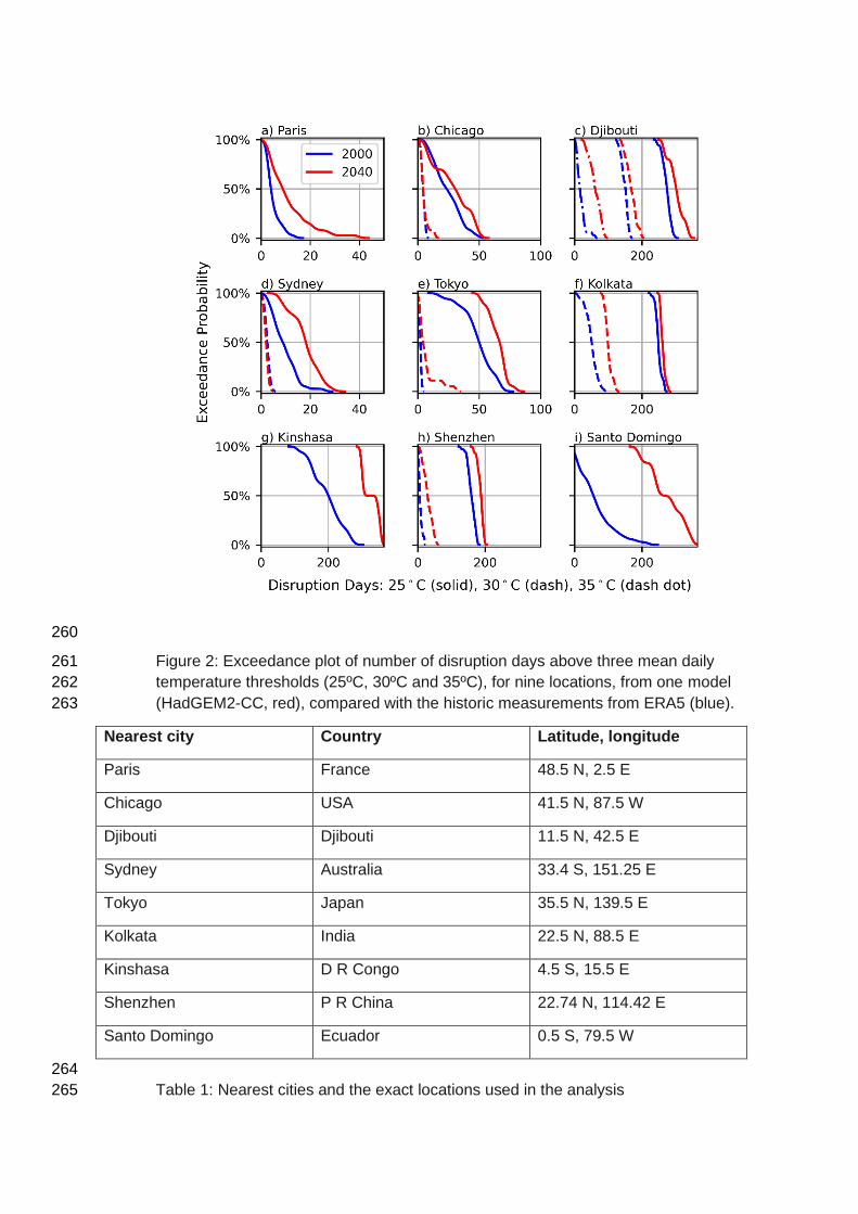
Figure 2 shows outputs for a single model (HadGEM2-CC, red line, centred on 2040) for 232
nine example locations from our global analysis, with up to three temperature thresholds 233
(25ºC, 30ºC and 35ºC), and compared with the ERA5 historic measurements (blue line, 234
centred on 2000). The nearest city locations to the actual analysed points are given in Table 235
1. These nine example locations were chosen in order to represent a broad geographic 236
spread of locations across all continents (excluding Antarctica). 237
The disruption days metric is based on specified mean daily temperature thresholds (25ºC, 238
30ºC and 35ºC in this case), and the probability of a threshold being exceeded in any given 239
year. This is shown on the vertical axes in Figure 2: for example, 10% exceedance 240
probability corresponds to a once-per-decade event, or 1% corresponds to a once-per-241
century event. These thresholds and exceedance probabilities can be adapted according to 242
the business assets in question, to match with the acceptable level of risk to the asset 243
operator, or to reflect the relevant regional context. 244
Figure 2 illustrates that the modelled future changes in the number of disruption days vary 245
widely by geographic location. For example, looking at the example of Paris in Figure 2a, we 246
see an increase of between 10 and 20 disruption days at the 25ºC threshold (solid line), for 247
low exceedance probabilities (i.e. 1-in-100 or 1-in-10 year events), but only a small increase 248
of just a few disruption days at higher exceedance probabilities. In contrast, for Santo 249
Domingo in Ecuador (Figure 2i), we see a large increase of over 100 disruption days for the 250
25ºC threshold at all exceedance probabilities. Kinshasa in DR Congo (Figure 2g) shows 251
similarly large increases in the number of disruption days at the 25ºC threshold. The other 252
locations in Figure 2 also show increases in the number of disruption days at the 30ºC 253
threshold (dashed line), and for some (e.g. Kolkata, Figure 2f), the modelled increase at the 254
30ºC threshold is greater than at the 25ºC threshold. For Djibouti (Figure 2c), we see the 255
greatest increase in number of disruption days at the 35ºC threshold (dashed-dotted line). 256
Recall that these thresholds illustrate the mean daily temperature, the peak daily 257
temperature will be significantly higher. The global variation in results is also clear from the 258
global maps shown in Figures 4 & 5. 259
260
Figure 2: Exceedance plot of number of disruption days above three mean daily 261
temperature thresholds (25ºC, 30ºC and 35ºC), for nine locations, from one model 262
(HadGEM2-CC, red), compared with the historic measurements from ERA5 (blue). 263
Nearest city Country Latitude, longitude
Paris France 48.5 N, 2.5 E
Chicago USA 41.5 N, 87.5 W
Djibouti Djibouti 11.5 N, 42.5 E
Sydney Australia 33.4 S, 151.25 E
Tokyo Japan 35.5 N, 139.5 E
Kolkata India 22.5 N, 88.5 E
Kinshasa D R Congo 4.5 S, 15.5 E
Shenzhen P R China 22.74 N, 114.42 E
Santo Domingo Ecuador 0.5 S, 79.5 W
264
Table 1: Nearest cities and the exact locations used in the analysis 265
Combining results from all models 266
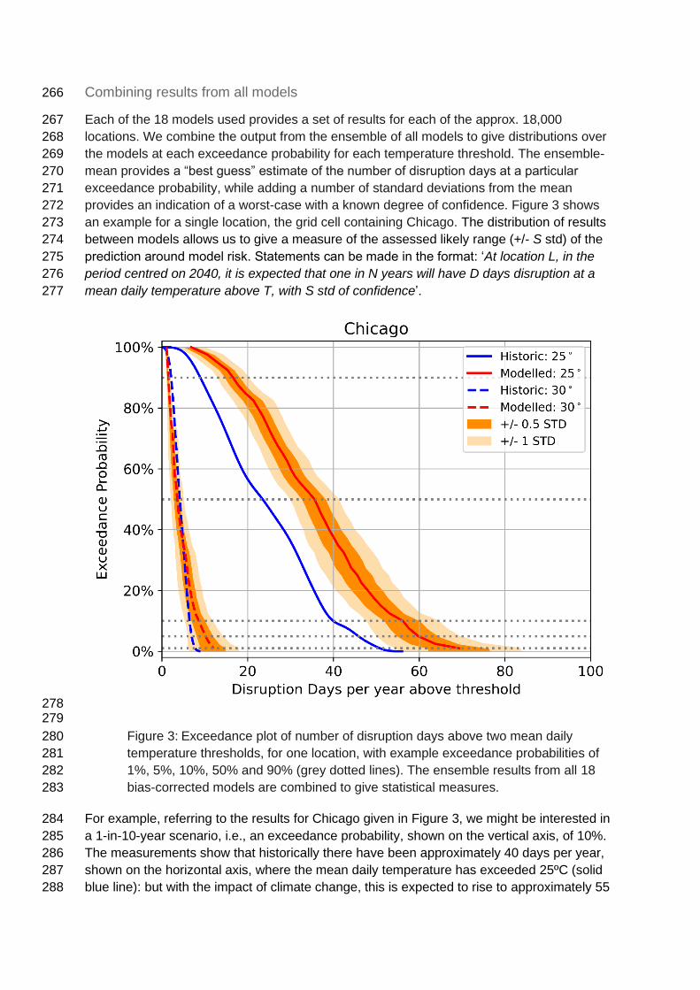
Each of the 18 models used provides a set of results for each of the approx. 18,000 267
locations. We combine the output from the ensemble of all models to give distributions over 268
the models at each exceedance probability for each temperature threshold. The ensemble-269
mean provides a “best guess” estimate of the number of disruption days at a particular 270
exceedance probability, while adding a number of standard deviations from the mean 271
provides an indication of a worst-case with a known degree of confidence. Figure 3 shows 272
an example for a single location, the grid cell containing Chicago. The distribution of results 273
between models allows us to give a measure of the assessed likely range (+/- S std) of the 274
prediction around model risk. Statements can be made in the format: ‘At location L, in the 275
period centred on 2040, it is expected that one in N years will have D days disruption at a 276
mean daily temperature above T, with S std of confidence’. 277
278 279
Figure 3: Exceedance plot of number of disruption days above two mean daily 280
temperature thresholds, for one location, with example exceedance probabilities of 281
1%, 5%, 10%, 50% and 90% (grey dotted lines). The ensemble results from all 18 282
bias-corrected models are combined to give statistical measures. 283
For example, referring to the results for Chicago given in Figure 3, we might be interested in 284
a 1-in-10-year scenario, i.e., an exceedance probability, shown on the vertical axis, of 10%. 285
The measurements show that historically there have been approximately 40 days per year, 286
shown on the horizontal axis, where the mean daily temperature has exceeded 25ºC (solid 287
blue line): but with the impact of climate change, this is expected to rise to approximately 55 288

days (solid red line). Therefore, we can say: ‘In Chicago for the period centred on 2040, we 289
expect every decade there will be one year where 55 days have a mean daily temperature 290
above 25ºC, up from 40 days for the period centred on 2000’. The uncertainty between 291
different models can be accounted for by the addition of the following statement: ‘there is a 292
16% chance that every decade one year will have 64 days exceeding this threshold’ 293
(corresponding to +1 std). This is essential for planning worst case scenarios and takes 294
account of model risk by incorporating an ensemble of results from different groups. 295
Although the change in absolute number of days may be quite small (55 disruption days 296
rather than 40), in a location which is historically ill-prepared for high temperatures, each day 297
can cause a significant cost and an increase in the fraction of days lost could be very 298
significant. One example might be locations in temperate regions that generally do not have 299
air conditioning, where the investment needed to install widespread building cooling capacity 300
would be very significant. 301
Another interpretation is to find the change in frequency for a given number of disruption 302
days. Referring again to Figure 3, there is approximately 10% probability (i.e. 1-in-10 year 303
expectation) of 40 disruption days with a mean daily temperature above 25ºC at the baseline 304
2000 condition. Under climate change, for the period centred on 2040 the same number of 305
disruption days is expected with about 38% likelihood, approximately 4-in-10 years. Thus, 306
we can expect approximately four times the number of years with this number of disruption 307
days. 308
This is often a more impactful way to understand the predictions. Risk and operation 309
managers and senior executives might be tempted to regard a 1-in-10 year expected loss as 310
simply a ‘risk of doing business’ which will generally be smoothed over with preceding and 311
following ‘normal’ years. If, however this loss approaches a 1-in-2 frequency, it will need to 312
be addressed, mitigated or provisioned. We believe that this method of presenting the 313
impacts of climate change is likely to promote meaningful change from operators and 314
owners of economic assets. 315
Global depiction of results 316
The examples above demonstrate the presented methodology for individual cities, with a 317
moderate temperature threshold. However, this technique is intended for a global application 318
to enable risk analysis of the exposures of global activities and value chains: the example of 319
Chicago above is also applicable to any global location. It is acknowledged that the use of an 320
absolute temperature threshold (e.g. 30ºC) has been criticised for not taking into account 321
climate variability (Zuo et al. 2015). However, we suggest that the application of critical 322
thresholds of disruption in this way is a useful method to assess global exposures in a 323
systematic way. Differences in the coping capacity of a specific region or locale to extreme 324
heat can be accounted for through variation of the vulnerability component of a risk 325
calculation. 326
Figure 4 shows a global map of the absolute number of disruption days over the 30ºC 327
threshold for the 2020-2059 period, at a 10% exceedance probability (one year in 10). For 328
each global location, the mean exceedance from all 18 of the bias corrected models is used. 329
It is clear from the map that for large parts of Saharan Africa, the Middle East and India, in 330

the period centred on 2040, it is expected that one-in-ten years will have a large number of 331
more than 200 dirsuption days per year over the 30ºC threshold, with some regions 332
experiencing up to 360 disruption days per year. A large number of disruption days is also 333
expected in Australia. Some parts of South America, in particular in the Amazon Basin, also 334
show a large number of disruption days. In other regions globally, including Europe, Sub-335
Saharan Africa and North America, the absolute number of expected disruption days per 336
year at the 30ºC threshold tends to be lower. However, while the absolute number of 337
disruption days may seem low in some regions, the increase in the number of disruption 338
days per year may still be higher. This is discussed in Figure 5. 339
340 Figure 4: Absolute number of daily mean disruption days per year over the 30ºC temperature 341
threshold for the 2020-2059 period, at a one-year-in-ten exceedance probability. 342
343
Figure 5 shows global maps of the expected increase in the number of disruption days from 344
1979-2018 to 2020-2059, using the threshold of mean daily temperature exceeding 25ºC, 345
30ºC and 35ºC, with a 10% probability of exceedance (i.e. one year each decade). 346
Differences in the impact between regions expected as a result of climate change can easily 347
be seen. For example, Central America and sub-Saharan Africa have a high increase in 348
daily mean 25ºC disruption days, but the greatest impact at 35ºC is in Saharan Africa and 349
the Middle East, which likely are close to exceeding lower temperature thresholds for most 350
days at historic conditions (illustrated for the example of Djibouti in Figure 2c). This 351
distinction is important, as a temperature threshold that is impactful in one region of the 352
world may be less relevant in another, demonstrating the need for regionally specific 353
thresholds. 354
355
356

357
358
Figure 5: Expected increase in the number of daily mean 25ºC (top), 30ºC (middle) 359
and 35ºC (bottom) disruption days from 1979-2018 to 2020-2059, at a one-year-in-360
ten exceedance probability, mean from all 18 bias-corrected models. 361
Maps such as these can be generated for any temperature or probability threshold, 362
incorporating if necessary a measure to account for uncertainty between the climate models, 363
by including a number of standard deviations from the mean between models at each 364
location, as illustrated for a single location (Chicago) in Figure 3. This approach can be 365
readily applied to risk assessment in a variety of domains, through analysis of the extreme 366
heat hazard against exposures and vulnerabilities of specific sectors, such as agriculture 367
(where agricultural risk models are used to calculate production disruption) or manufacturing 368
(e.g. to assess rates of absenteeism/presenteeism, reduction of output, energy demands 369
and air conditioning loads, etc.). 370
Aggregated global results 371
Although the primary focus of this paper is on providing localised estimations of the change 372
in disruption days, it is also interesting to get a broad measure of the global change in 373
disruption days. To do so, we divide the globe into three zones by latitude: 0º to 23.5º 374
(‘tropical’), 23.5º to 35.5º (‘sub-tropical’) and 35.5º to 70º (‘temperate’). For each land-mass 375
grid square in each zone and at each temperature threshold, we calculate the mean of the 376
baseline number of disruption days and the mean of the increase in disruption days 377
expected from 1979-2018 to 2020-2059. The results are shown in Table 2. 378
379

Threshold temp
(daily mean)
Zone Mean baseline number
of disruption days for
1979-2018
Mean increase in number
of disruption days from
1979-2018 to 2020-2059
25ºC Tropical 237 39
Sub-tropical 125 20
Temperate 16 8
30ºC Tropical 51 26
Sub-tropical 56 20
Temperate 5 6
35ºC Tropical 17 19
Sub-tropical 19 12
Temperate 1.3 4.2
Table 2: Mean number of disruption days, and mean increase, for three latitude zones at 380
three temperature thresholds 381
This averaged analysis of course hides a large amount of local data: some localities will 382
have a much larger increase in the number of disruption days and some may have no 383
increase or even a slight decrease (for example some regions of Russia and Canada show a 384
decrease in Figure 5). 385
Given the wide distribution in the increase in the number of disruption days, a more 386
informative way to analyse the data is to ask what fraction of locations in each zone have 387
more than a given number of days increase. We show this fraction in Table 3 for the same 388
temperature thresholds and latitude zones, for 10 and 30 days. 389
Threshold temp
(daily mean)
Zone Fraction of locations with
more than 10 disruption
days increase
Fraction of locations with
more than 30 disruption
days increase
25ºC Tropical 77% 44%
Sub-tropical 82% 12%
Temperate 20% 1%
30ºC Tropical 64% 28%
Sub-tropical 66% 16%
Temperate 7% 0%
35ºC Tropical 24% 12%
Sub-tropical 29% 7%
Temperate 1% 0%
Table 3: Fractional increase in the number of locations predicted to have 10 and 30 390
additional disruption days, for three latitude zones at three temperature thresholds 391
Tropical regions are impacted the most with highest fraction of locations suffering 30 392
additional days. For 10 days, sub-tropical regions are approximately equally affected, with 393
temperate latitudes the least impacted. It is worth remembering though that temperate 394
regions may have the biggest financial sensitivity to the disruption days, since many 395
locations will be relatively poorly prepared. 396
397

Discussion 398
Although in some cases the absolute increase in the number of disruption days in the results 399
discussed above is relatively small, we must remember that: 400
• This analysis is performed on daily mean temperatures, so a daily peak temperature 401
will be significantly higher. 402
• Economic processes slow down very rapidly with rising temperature, so (for instance) 403
the prospect of a threefold increase in the number of economically unproductive days 404
would be highly impactful. 405
• The strong variation between locations (illustrated in Figures 2 & 5) shows that this 406
mean increase includes many locations with a much higher increase. 407
• Some locations will be less prepared than others. For example, housing and 408
workspaces in many temperate locations do not have air cooling. As a result, an 409
increase in the number of days at even a low temperature threshold could have a 410
higher economic impact than at a sub-tropical location, where at least there is a 411
higher level of preparedness to hot days. 412
Localised Economic Impacts 413
Extreme climate events are known to cause devastating damage, both in human lives and in 414
financial assets. The future ‘climate value at risk’ of global financial assets is US$2.5 trillion 415
in the ‘business-as-usual’ scenario, while the 99th percentile of the possible outcomes gives 416
the value of approximately US$24.2 trillion (Dietz et al. 2016). In addition, climate-economic 417
models show that loses from climate change may reach 23% of the global gross product by 418
the end of the 2100 (Klusak et al., 2021; Burke et al., 2015). Over the past 40 years (since 419
1980), estimations show that weather-related natural disasters alone caused losses of 420
around US$4.2 trillion and claimed approximately 1 million lives (Munich Re, 2021). 421
Heatwaves have shown increasing trends in frequency, duration and cumulative heat since 422
the mid-twentieth century, and have also shown signs of acceleration of those trends in the 423
presence of global warming (Perkins-Kirkpatrick and Lewis, 2020). Those upward trends can 424
be seen in the recent past of such events - the major European heat waves of 2003 and 425
2019 were just 16 years apart but were estimated to be 1-in-450 years and 1-in-283 years 426
events respectively (Munich Re, 2004; Ma et al., 2020). Those types of events can be 427
catastrophic for people, countries and businesses, especially if mitigation plans are not in 428
place. The 2003 European heat wave claimed an estimated 35,000 lives, 14,947 out of 429
those in France alone, a country without a strategy against heat waves at the time (Larsen 430
2003, Poumadère et al., 2005). Estimates of the financial cost for this event alone are 431
around US$13 billion, mostly in agricultural costs, which is believed to be a conservative 432
estimate as crops were not usually insured in Europe in 2003 (Munich Re, 2004; De Bono et 433
al., 2004). 434
Providing economic loss calculations due to future heat waves is outside the scope of this 435
paper, but the methods and results showcased in this study can provide a good baseline for 436
such estimations. For example, making an assumption that the 1995 Chicago heat wave 437
was a 1-in-100 years event (Karl and Knight, 1997) and the fact that this event is part of the 438
1979-2018 timeseries, one can use our disruption days framework to estimate the probability 439

of a similar event arising in the 2040-centered period. Reading from Figure 3, in terms of the 440
same number of disruption days (both 25ºC and 30ºC thresholds), the probability of having a 441
similar event would increase to 10% (or 1-in-10 years). This result is limited by the 442
aforementioned assumption, but also by the assumption that the ‘disruption days per year’ 443
metric is perfectly correlated with the emergence of heat waves. The lack of higher precision 444
in distributions of this metric can also have an effect on this result as the smallest increment 445
in our exceedance probability plots is 2.5%, while the event is assumed to have a probability 446
of 1%. However, this result does show the potential of this type of analysis for the mitigation 447
of future extreme weather events. 448
By knowing the sensitivity to temperatures and the geographic distribution of their 449
operations, it becomes feasible for an organization or business to quantify their expected 450
total financial loss due to temperature disruption days. This could be essential for 451
provisioning, insurance or risk reporting, including TCFD disclosures. It also lays the 452
foundations for planning strategic responses to physical climate change risk. 453
Future Work 454
The procedures described in this paper give the first stage of assessing a financial cost at a 455
relatively local resolution from extreme temperature effects, expressed as “disruption days”. 456
However, it needs to be followed by assessments at a local level of economic vulnerability to 457
disruption days. These could be as simple as “the airport will close if the mean daily 458
temperature is above 35ºC” or “the cost of electricity generation for the region rises by 459
US$50 million for each day above 30ºC”. At the other extreme, a complex, multi-location 460
operation could assess operations at each location, and apply these vulnerabilities to the 461
disruption days calculated here to give a total expected additional cost. By combining all 462
significant economic activity in a region and estimating vulnerability to extreme weather, it 463
would be possible for a local or national government to estimate the gross effect of 464
temperature disruption days on their economy. A multinational company with economically 465
productive assets spread over many locations could do the same. 466
The general approach used in this study (re-gridding at relatively fine spatial granularity, bias 467
correction of individual models, calculation of the disruption days for each model at each 468
location, followed by ensemble averaging over models to get model risk statistics) can 469
equally well be applied to other extreme weather features which are likely to be affected by 470
climate change, and could be the subject of future work: 471
472
● Precipitation. Droughts and flooding have profound effects on many natural and 473
human activities, not least agriculture. 474
● Multivariate analysis of compound risks. For example, the impacts of humidity 475
combined with temperature, or drought combined with high temperature. 476
● Low temperature thresholds. Frost days, for example, can limit economic activity in 477
some temperate regions, where freezing temperatures are relatively rare and 478
preparedness is low. 479
● Quantifying maximum or minimum daily temperatures, rather than mean daily 480
temperatures, might also be interesting as many activities are more accurately limited 481
by daily extremes rather than mean temperatures. 482
483

The methodological analysis presented in this paper could be improved in future studies as 484
and when new datasets and methods become available. In terms of data preparation and 485
pre-analysis, machine learning methods show great promise in improving existing bias 486
correction techniques, and such new methods could be applied to repeat and improve our 487
analysis presented here. While this study has focussed on the use of model results from the 488
CMIP5 generation of climate models, the newly available generation of CMIP6 models have 489
a higher spatial resolution and would allow for the approach in this paper to be repeated with 490
finer geographic grids. 491
Conclusion 492
Using multi-model, bias-corrected results from CMIP5 climate models we estimate the 493
frequency of daily mean temperatures exceeding certain temperature thresholds on 494
“disruption days”, at given locations for a future period centred on 2040, compared with 495
historical observations from ERA5 centred on 2000. Since it is often the exceedance over a 496
threshold, rather than simply the mean annual temperature, that is the determining factor for 497
economic activity, this approach is expected to be a better indicator on the effect of climate 498
change on human and economic activity. 499
Our results allow for the estimation of the increase in the number of disruption days 500
exceeding a certain temperature threshold for a given location and exceedance probability. 501
For example, in Chicago one can expect that by 2040, every decade there will be one year 502
where 55 days have a mean daily temperature above 25ºC, up from 40 days for the period 503
centred on 2000. Another way to read the results is that Chicago can expect a fourfold 504
increase in the number of years with at least 40 disruption days above the 25ºC threshold by 505
2040. 506
Globally, our results also show that there is broad variation in the modelled increase in 507
number of disruption days, for different locations, temperature thresholds and exceedance 508
probabilities. Central America and Sub-Saharan Africa show the largest increases in number 509
of disruption days at the 25ºC temperature threshold, while the greatest increases in 510
disruption days exceeding 35ºC are seen in Saharan Africa and the Middle East. 511
By combining these results with the sensitivities of economic activities to temperature 512
thresholds, it becomes possible to estimate the financial impact of climate change on a wide 513
variety of businesses. Examples are logistics (frequently disrupted by weather extremes), 514
outdoor work (where human productivity rapidly falls with temperature) and agricultural 515
yields (which typically fall once a crop-dependant temperature threshold is passed). 516
By knowing locations and the nature of activities through an organisation, it will be possible 517
to estimate, with a given level of confidence over model risk, the financial impact of climate 518
change related changes in temperature. 519
520
Acknowledgement 521
The authors would like to express gratitude to Professor Daniel Ralph and Mr Oliver 522
Carpenter at The Centre for Risk Studies, University of Cambridge, Judge Business School. 523
524
Appendix 525
The CMIP5 models used are: ACCESS1-3, BNU-ESM, CMCC-CMS, CNRM-CM5, CSIRO-526
Mk3-6, GFDL-CM3, GFDL-ESM2G, GFDL-ESM2M, HadGEM2-CC, HadGEM2-ES, IPSL-527
CM5A-LR, IPSL-CM5A-MR, IPSL-CM5B-LR, MPI-ESM-LR, MPI-ESM_MR, NorESM1-M, 528
bcc-csm1-1 and inmcm4. A small number of other models were not included either because 529
they had been superseded by later models from the same research group or because of 530
data incompatibilities. 531
532
References 533
Burke, Marshall, Solomon M. Hsiang, and Edward Miguel. "Global non-linear effect of 534 temperature on economic production." Nature 527, no. 7577 (2015): 235-239. 535
Ciavarella. (2020). Prolonged Siberian heat of 2020. Retrieved 10 25, 2020, from 536 https://www.worldweatherattribution.org/wp-content/uploads/WWA-Prolonged-heat-537 Siberia-2020.pdf 538
Dietz, Simon, Alex Bowen, Charlie Dixon, and Philip Gradwell. "‘Climate value at 539
risk’ of global financial assets." Nature Climate Change 6, no. 7 (2016): 540
676-679. 541
De Bono, Andréa, Pascal Peduzzi, Stéphane Kluser, and Gregory Giuliani. "Impacts of 542 summer 2003 heat wave in Europe." (2004). 543
Eccles, R. &. Krzus, M. (2018). Why Companies Should Report Financial Risks From 544 Climate Change. MIT Sloan Management Review, 59(3), 1-6. 545
Gudmundsson, Lukas, John Bjørnar Bremnes, Jan Haugen, and T. Skaugen. 2012. 546 ‘Technical Note: Downscaling RCM Precipitation to the Station Scale Using Quantile 547 Mapping – A Comparison of Methods’. Hydrology and Earth System Sciences 548 Discussions 9 (May): 6185–6201. https://doi.org/10.5194/hessd-9-6185-2012. 549
Haerter, J. O., S. Hagemann, C. Moseley, and C. Piani. 2011. ‘Climate Model Bias 550 Correction and the Role of Timescales’. Hydrology and Earth System Sciences 15 551 (3): 1065–79. https://doi.org/10.5194/hess-15-1065-2011. 552
Handmer, John, Yasushi Honda, Zbigniew W. Kundzewicz, Nigel Arnell, Gerardo Benito, 553 Jerry Hatfield, Ismail Fadl Mohamed, et al. 2012. ‘Changes in Impacts of Climate 554 Extremes: Human Systems and Ecosystems’. In Managing the Risks of Extreme 555 Events and Disasters to Advance Climate Change Adaptation, edited by Christopher 556 B. Field, Vicente Barros, Thomas F. Stocker, and Qin Dahe, 231–90. Cambridge: 557 Cambridge University Press. https://doi.org/10.1017/CBO9781139177245.007. 558
Hawkins, Ed, Thomas M. Osborne, Chun Kit Ho, and Andrew J. Challinor. 2013. ‘Calibration 559 and Bias Correction of Climate Projections for Crop Modelling: An Idealised Case 560 Study over Europe’. Agricultural and Forest Meteorology, Agricultural prediction using 561 climate model ensembles, 170 (March): 19–31. 562 https://doi.org/10.1016/j.agrformet.2012.04.007. 563
Hempel, Sabrina, Katja Frieler, Lila Warszawski, Jacob Schewe, and Franziska Piontek. 564 2013. ‘A Trend-Preserving Bias Correction – The ISI-MIP Approach’. Earth System 565 Dynamics Discussions 4 (January): 49. https://doi.org/10.5194/esdd-4-49-2013. 566
Hersbach, Hans, Bill Bell, Paul Berrisford, Shoji Hirahara, András Horányi, Joaquín 567 Muñoz‐Sabater, Julien Nicolas, et al. 2020. ‘The ERA5 Global Reanalysis’. Quarterly 568 Journal of the Royal Meteorological Society 146 (730): 1999–2049. 569 https://doi.org/10.1002/qj.3803. 570
IPCC. 2018. ‘Summary for Policymakers — Global Warming of 1.5 oC’. 2018. 571 https://www.ipcc.ch/sr15/chapter/spm/. 572

Karl, Thomas R., and Richard W. Knight. "The 1995 Chicago heat wave: How likely is a 573 recurrence?." Bulletin of the American Meteorological Society 78, no. 6 (1997): 1107-574 1120. 575
Kew, Sarah, Sjoukje Philip, Geert Jan van Oldenborgh, Amalie Skålevåg, and Philip Lorenz. 576 2020. ‘Prolonged Siberian Heat of 2020’, 35. 577
Larsen, Janet. "Record heat wave in Europe takes 35,000 lives: Far greater losses may lie 578 ahead." Earth Policy Institute (2003). 579
Poumadere, Marc, Claire Mays, Sophie Le Mer, and Russell Blong. "The 2003 heat wave in 580 France: dangerous climate change here and now." Risk Analysis: an International 581 Journal 25, no. 6 (2005): 1483-1494. 582
Klusak, Patrycja, Matthew Agarwala, Matt Burke, Moritz Kraemer, and Kamiar Mohaddes. 583 "Rising temperatures, falling ratings: The effect of climate change on sovereign 584 creditworthiness." (2021). 585
Ma, Feng, Xing Yuan, Yang Jiao, and Peng Ji. "Unprecedented Europe heat in June–July 586 2019: risk in the historical and future context." Geophysical Research Letters 47, no. 587 11 (2020): e2020GL087809. 588
Maraun, Douglas. 2013. ‘Bias Correction, Quantile Mapping, and Downscaling: Revisiting 589 the Inflation Issue’. Journal of Climate 26 (6): 2137–43. https://doi.org/10.1175/JCLI-590 D-12-00821.1. 591
Maraun, Douglas, Theodore G. Shepherd, Martin Widmann, Giuseppe Zappa, Daniel 592 Walton, José M. Gutiérrez, Stefan Hagemann, et al. 2017. ‘Towards Process-593 Informed Bias Correction of Climate Change Simulations’. Nature Climate Change 7 594 (11): 764–73. https://doi.org/10.1038/nclimate3418. 595
Maraun, Douglas, and Martin Widmann. 2018. Statistical Downscaling and Bias Correction 596 for Climate Research. Cambridge: Cambridge University Press. 597 https://doi.org/10.1017/9781107588783. 598
Mora, Camilo, Bénédicte Dousset, Iain R. Caldwell, Farrah E. Powell, Rollan C. Geronimo, 599 Coral R. Bielecki, Chelsie W. W. Counsell, et al. 2017. ‘Global Risk of Deadly Heat’. 600 Nature Climate Change 7 (7): 501–6. https://doi.org/10.1038/nclimate3322. 601
Munich Re. "TOPICS geo 2003." Mü nchener Rü ckverischerungs-Gessellschaft, Munich 602 (2004). 603
Oldenborgh, Geert Jan van, Folmer Krikken, Sophie Lewis, Nicholas J. Leach, Flavio 604 Lehner, Kate R. Saunders, Michiel van Weele, et al. 2020. ‘Attribution of the 605 Australian Bushfire Risk to Anthropogenic Climate Change’. Natural Hazards and 606 Earth System Sciences Discussions, March, 1–46. https://doi.org/10.5194/nhess-607 2020-69. 608
Silverman, B.W. (1986). Density Estimation for Statistics and Data Analysis. London: 609 Chapman & Hall/CRC. p. 45. ISBN 978-0-412-24620-3. 610
Simpson, C, Hosking, J S, Mitchell, D, Betts, R A, and Shuckburgh, E. 2021. ‘Regional 611 Disparities in Climate Risk to Rice Labour and Food Security’. Submitted to 612 Environmental Research Letters, Preprint: https://doi.org/10.31223/X5SW3N. 613
TCFD. 2020. ‘2020 Status Report’. Task Force on Climate-Related Financial Disclosures. 614 2020. https://www.fsb.org/2020/10/2020-status-report-task-force-on-climate-related-615 financial-disclosures/. 616
———. 2020. ‘Support TCFD’. Task Force on Climate-Related Financial Disclosures (blog). 617 2020. https://www.fsb-tcfd.org/support-tcfd/. 618
Wouters, Hendrik, Koen De Ridder, Lien Poelmans, Patrick Willems, Johan Brouwers, 619 Parisa Hosseinzadehtalaei, Hossein Tabari, Sam Vanden Broucke, Nicole P. M. 620 van Lipzig, and Matthias Demuzere. 2017. ‘Heat Stress Increase under Climate 621 Change Twice as Large in Cities as in Rural Areas: A Study for a Densely Populated 622 Midlatitude Maritime Region’. Geophysical Research Letters 44 (17): 8997–9007. 623 https://doi.org/10.1002/2017GL074889. 624
Xia, Yang, Yuan Li, Dabo Guan, David Mendoza Tinoco, Jiangjiang Xia, Zhongwei Yan, Jun 625 Yang, Qiyong Liu, and Hong Huo. 2018. ‘Assessment of the Economic Impacts of 626

Heat Waves: A Case Study of Nanjing, China’. Journal of Cleaner Production 171 627 (January): 811–19. https://doi.org/10.1016/j.jclepro.2017.10.069. 628
Zuo, Jian, Stephen Pullen, Jasmine Palmer, Helen Bennetts, Nicholas Chileshe, and Tony 629 Ma. 2015. ‘Impacts of Heat Waves and Corresponding Measures: A Review’. Journal 630 of Cleaner Production 92 (April): 1–12. https://doi.org/10.1016/j.jclepro.2014.12.078. 631
632