Local Volatility Modeling of JSE Exotic Can-Do Options

Antonie Kotzea, Rudolf Oosthuizenb, Edson Pindzac

aSenior Research Associate, Faculty of Economic and Financial SciencesDepartment of Finance and Investment Management, University of Johannesburg

PO Box 524, Aucklandpark 2006, South AfricabThe JSE, One Exchange Square, Gwen Lane, Sandown, 2196, South Africa

Tel: +2711-520-7000cUniversity of Pretoria

Number of pages: 46Date: 1 July 2014

Abstract

Can-Do Options are derivative products listed on the JSE’s derivative exchanges — mostlyequity derivative products listed on Safex and currency derivative products listed on Yield-X. These products give investors the advantages of listed derivatives with the flexibilityof “over the counter” (OTC) contracts. Investors can negotiate the terms for all optioncontracts, choosing the type of option, underlying asset and the expiry date. Many exoticoptions and even exotic option structures are listed. Exotic options cannot be valued usingclosed-form solutions or even by numerical methods assuming constant volatility. Mostexotic options on Safex and Yield-X are valued by local volatility models. Pricing underlocal volatility has become a field of extensive research in finance and various models areproposed in order to overcome the shortcomings of the Black-Scholes model that assumesthe volatility to be constant.

In this document we discuss various topics that influence the successful constructionof implied and local volatility surfaces in practice. We focus on arbitrage-free conditions,choice of calibrating functionals and selection of numerical algorithms to price options.We illustrate our methodologies by studying the local volatility surfaces of South Africanindex and foreign exchange options. Numerical experiments are conducted using Excel andMATLAB.

Keywords: Exotic options, JSE, Can-Do Options, Implied Volatility, Local Volatility,Dupire Transforms, Gyongy Theorem, Markov Projection

(JEL) Classification: C61, G17

Email addresses: antonie@quantonline.co.za; http://www.quantonline.co.za (AntonieKotze), rudolfo@jse.co.za (Rudolf Oosthuizen), pindzaedson@yahoo.fr (Edson Pindza)

1

Contents

1 Introduction 3

2 Black-Scholes Partial Differential Equations 52.1 Assuming Constant Volatility . . . . . . . . . . . . . . . . . . . . . . 52.2 Consistency with the Volatility Skew . . . . . . . . . . . . . . . . . . 6

3 Local volatility 73.1 Rubinstein’s Thoughts . . . . . . . . . . . . . . . . . . . . . . . . . . 83.2 The Similarity with Forward Rates . . . . . . . . . . . . . . . . . . . 93.3 What does it Mean in Practice? . . . . . . . . . . . . . . . . . . . . . 12

3.3.1 Implied and Instantaneous Volatility . . . . . . . . . . . . . . 123.3.2 Local Volatility by Example . . . . . . . . . . . . . . . . . . . 153.3.3 Sticky Local Volatility . . . . . . . . . . . . . . . . . . . . . . 17

3.4 Local Volatility by a Deterministic Volatility Function . . . . . . . . . 193.5 Dupire Local Volatility . . . . . . . . . . . . . . . . . . . . . . . . . 193.6 Local Volatility in terms of Implied Volatility . . . . . . . . . . . . . 23

4 The ALSI: Exact Implementation 244.1 The Deterministic Implied Volatility Function . . . . . . . . . . . . . 244.2 The ALSI Implied and Local Volatilities . . . . . . . . . . . . . . . . 27

5 Numerical Implementation of Dupire 295.1 Volatility Interpolation and Extrapolation . . . . . . . . . . . . . . . 295.2 Safex’s Implementation . . . . . . . . . . . . . . . . . . . . . . . . . . 315.3 Comparing the Implied and Local Volatilities for Dtop and Usdzar . . 355.4 Dupire in terms of Call Prices . . . . . . . . . . . . . . . . . . . . . . 35

6 Conclusion 36

Appendices 38

A Derivation local volatility formula 38A.1 Dupire local volatility . . . . . . . . . . . . . . . . . . . . . . . . . . . 38A.2 Local Volatility by Implied Volatility . . . . . . . . . . . . . . . . . . 40

B Gyongy’s Theorem and Markov Projection 41

2

1. Introduction

One of the central ideas of economic thought is that, in properly functioningmarkets, prices of traded goods contain valuable information that can be used tomake a wide variety of economic decisions. In financial derivative markets, impliedvolatility is one such traded quantity. The expected future value of traded volatilityplays a central role in finance theory. It is thus crucial to estimate this parameteraccurately enabling meaningful financial decision making.

In finance, the volatility is defined as a variational measure of price of a givenfinancial instrument over time. There exist many types of volatilities classified us-ing different standards. For instance, the historical or realised volatility is a type ofvolatility derived from time series based on the past market prices. Implied volatil-ity, however, is a type of volatility derived from the market — obtained from tradedderivatives like options — while local or instantaneous volatility is not directly mea-surable from the market nor from historical data. Black and Scholes assumed volatilityto be constant over the life of an option which was helpful in deriving the seminalBlack-Scholes formula for option prices — remember, there were other importantassumptions as well (see Hull (2012); Kotze (2003); Black (1988)).

Practitioners and quants know that the assumption of constant volatility is wrong.The evidence to this is the long-observed pattern of implied volatilities, where at-the-money and in-the-money options tend to have lower implied volatilities than out-of-the-money options for equities. This pattern is called the volatility skew. Impliedvolatility for currency options, on the other hand, has a smile pattern where in-the-money and out-the-money options have higher implied volatilities than at-the-moneyoptions.

One explanation for this phenomenon is that, in reality, the assumed randomnature of asset prices is plainly wrong. Asset prices thus do not diffuse throughtime in a random manner implying the probability distribution of asset prices is notlog-normal. Market practitioners rectify (or modify) the Black-Scholes assumptionof geometric Brownian motion by trading options with different strikes at differentvolatilities. The fact that volatility is not constant has ramifications when path-dependent options are priced. These products do not just depend on the variabilityof the underlying asset’s price, but also on the variability of the volatility. Nowremember, the choice of which model to use depends on the different risks involvedin the option (Bouzoubaa & Osserein, 2010). Path-dependent options thus has skewdependence or they are skew-sensitive. We need to use models that capture this effectand that prompt the development of various volatility models as an alternative to theBlack-Scholes model. In particular, stochastic volatility models (Heston, 1993; Hull& White, 1993), local volatility models (Coleman et al., 1999; Dupire, 1994; Derman& Kani, 1994), jump-diffusion models (Kou, 2002; Merton, 1976) and Levy models(Madan & Seneta, 1990) amongst others were developed.

In this paper, we consider the local volatility approach to value a new range oflisted exotic products called Can-Do options — this product range was launched bythe Johannesburg Stock Exchange (JSE) on 8 January 2007. Can-Do options aresimilar to CBOE’s Flex option range of products. It started out where clients wanted

3

to have the ability to customise key contract terms like the expiry date. However,the suite of products quickly grew to include exotic options and structured products1.Kotze & Oosthuizen (2013) discuss and explain the local volatility pricing of exoticCan-Do options like Barrier options, as well as the methodologies used to determinetheir initial margins. Local volatility models have been in use since the 1980s althoughthese were not known by the name “local volatility.” The mathematical framework forlocal volatility was first formulated by Dupire (1994). At the same time, Derman &Kani (1994) and Rubinstein (1994) solved this problem numerically by implementingbinomial trees. These methods have subsequently been improved by many otherresearchers (Andersen & Andreasen, 2000; Lagnado & Osher, 1997). It has sincebeen realised that Dupire’s framework is an extension of research done by Gyongy(1986).

The local volatility functional approach has become popular with practitioners,because of its simplicity and the fact that it conveniently retains the market complete-ness2 of the Black-Scholes model and it is consistent3. Due to this the Black-Scholesmodel is a convenient translation mechanism. It is universally used by traders to“talk” to one another; it gives unambiguous answers. It further retains the intuitiveconcept of the implied volatility skew where the implied volatility is a function of thestrike and time only — it is non-stochastic. Similar to this parameterisation, the localvolatility is also a function of strike and time. Moreover, the existence of a forwardequation that describes the evolution of call option prices as functions of maturitytime and strike price makes it possible to express the unknown volatility functiondirectly in terms of known option prices. It thus captures the implied volatility skewwithout introducing additional sources of risk. This is different to stochastic volatilitymodels which assume the volatility follows a random process as well.

Some local volatility parameterisations have one practical problem that needs tobe addressed. In the real market, there exist a limited number of accessible datapoints (traded volatilities or volatility bids and offers). When implementing the localvolatility models, one might have to estimate values between two consecutive givendata points. This is overcome by interpolation. There are two ways this can be done:either smooth the data points by fitting a functional form (like a quadratic function)or find an interpolation technique that works (simplest being linear interpolation).However, using the incorrect interpolation technique can be dangerous in that it canyield arbitrage opportunities. Therefore it is important to consider practical arbi-trage free techniques to construct volatility surfaces. This paper gives an overview ofsuch approaches, describes characteristics of volatility surfaces and provides practicaldetails for the construction of volatility surfaces.

The rest of this paper is organized as follows. In Section 2, we describe theformulation of the Black-Scholes partial differential equation and show how it can be

1http://www.jse.co.za/Products/Equity-Derivatives-Market/

Equity-Derivatives-Product-Detail/Can-Do_Futures_and_Options.aspx2It allows hedging based on the underlying asset alone.3It has no contradictions i.e., the price is the price. If two traders use the same input values, the

answers will be the same, exactly.

4

made to incorporate the implied volatility skew. This section can be skipped if thereader do not want to re-read the mathematical rigors of the Black-Scholes theory.Section 3 reviews the concept of local volatility and explains it from a practicalperspective. We introduce the Dupire formulation using Dupire’s mapping betweenimplied and local volatility and discuss the numerical implementation thereof. Section4 introduces the functional implementation for the Alsi implied volatility surface andwe show how the Dupire framework can be used to obtain the corresponding localvolatility surface algebraically. In Section 5 we show how the local volatility surfacecan be obtained numerically for the DTOP index and USDZAR exchange rate. Weconclude in Section 6.

2. Black-Scholes Partial Differential Equations

This section discusses the mathematical background and can be skipped

We want to determine the price of a security that guarantees a payment h(·)contingent on the state of the process S at maturity date T . For a call optionh(S) = max[S −K, 0] where K is called the strike price.

In the Black-Scholes framework, we start by assuming that the security priceS evolves log-normally, according to the following stochastic differential equation(Wilmott, 1998)

dS

S= µdt+ σdW (2.1)

where µ is the expected continuously compounded rate of return earned by an investorin a short period of time dt — the instantaneous expected return. Further, σ is theinstantaneous volatility or standard deviation of return from the security price S, andW is a standard Brownian motion or Wiener process, with mean zero and varianceequal to 1. A geometric Brownian motion is a natural two-parameter model of asecurity-price process because of the simple interpretations of µ and σ (Duffie, 1996).Note that W , and consequently its infinitesimal increment dW , represents the onlysource of uncertainty in the price history of the security.

2.1. Assuming Constant Volatility

Black, Scholes and Merton made some assumptions in order to facilitate a betterunderstanding of the dynamics of the security price S. One of the main assumptions isthat of risk neutrality. In its simplest form, this infers that all risk-free portfolios canbe assumed to earn the same risk-free rate. They further assumed that the volatilityin equation (2.1) is deterministic (constant) and the discount rate is the constantrisk-free rate r. Under these assumptions, the risk-neutral dynamic of the asset is(Hull, 2012)

dSt = (r − d)Stdt+ σ(K,T )StdWt. (2.2)

where Wt is a standard Brownian motion or Wiener process, St denotes a risky under-lying asset price process at time t and d is the constant dividend rate. εquation (2.2)

5

describes a simple one-factor asset price process where σ(K,T ) is called the impliedvolatility and it is a function of the fixed strike K and expiry time T only.

Let the scalar function Vbs(S, t) be the value of a contingent claim like an optionat any time t conditional on the price of the underlying being S at that time. UsingIto’s lemma, εquation (2.2) can be transformed to the Black-Scholes stochastic partialdifferential equation (PDE)

∂Vbs∂t

+1

2σ2(K,T )S2∂

2Vbs∂S2

+ (r − d)S∂Vbs∂S− rVbs = 0. (2.3)

εquation (2.3) basically describes how the value of a derivative contract, at a con-tinuum of potential future scenarios, diffuses backwards in time towards today. Thisequation is a backward parabolic partial differential equation also known as the back-ward Kolmogorov equation.

Under the assumption of a constant volatility σ(K,T ), this PDE can be solvedanalytically by applying the Feynman-Kac theorem and resulting formula (Castagna,2010). This formula establishes a link between parabolic partial differential equationsand stochastic processes. It offers a method of solving certain PDEs by simulatingrandom paths of a stochastic process (Klebaner, 2005; Clark, 2011). The solution ofεquation (2.3) with the terminal condition Vbs(ST , T ) = max[ST −K, 0] where ST isthe underlying’s price at time T , gives the seminal Black-Scholes formula.

Please note that εquation (2.3) is solved backwards in time — the terminal con-ditions are specified and the solution today is sought (Clark, 2011). Even though theBlack-Scholes formula is the solution to a very specific and simple PDE, it is still veryrelevant.

One crucial point one has to understand is that the implied volatility, σ(K,T ) inεquation (2.3) is not linked in any simple way to the volatility, σ, of the true stockprice process described in εquation (2.1). The implied volatility is not the standarddeviation of S. This led to the famous statement by Rebonato (2004):

“Implied volatility is the wrong number to put into the wrong formula toget the right price of plain-vanilla options.”

Implied volatilities are simply a short-hand notation to quote a price! This impliesthat

σ(K,T )2T 6=∫ T

0

σ(Su, u)2du (2.4)

where σ(St, t) is the instantaneous volatility of the stochastic process St. Impliedvolatilities are not volatilities after all (neither instantaneous nor average)!

2.2. Consistency with the Volatility Skew

Although satisfactory for European options, the Black-Scholes model comes upshort for more complex options, such as Asian options (whose payoff depends on theaverage price of the underlying asset over time), barrier options (whose value dependson whether a specific boundary value has been attained by the underlying asset beforeits maturity) or even common American options.

6

Practitioners thus started looking for a simple way of pricing more complex op-tions. The prerequisite was that the methodology should be consistent with thevolatility skew. If we now generalise εquation (2.2) and assume that volatility is de-pendent on the asset’s price and time (it’s not constant anymore) but we still assumeit to be deterministic, we get

dSt = (r − d)Stdt+ σ(St, t)StdWt. (2.5)

Here, the function σ(S, t) is called the local volatility function because it is dependenton both S and t. Note that σ(t) is sometimes referred to as the instantaneous volatility— it is a function of time only.

Using Ito’s lemma and the scalar function Vl(S, t) (the value of an option), εquation(2.5) can be transformed to the generalised Black-Scholes PDE

∂Vl(S, t)

∂t+

1

2σ2(S, t)S2∂

2Vl∂S2

+ (r − d)S∂Vl∂S− rtVl = 0. (2.6)

If Vl(S, t) is twice differentiable and Vl(ST , T ) is the terminal condition, the Feynman-Kac theorem states that the solution to this backward parabolic partial differentialequation shown in εquation (2.6) is given by

Vl(S, t) = EQ[e−

∫ Tt ruduVl(ST , T )|St = S

], (2.7)

where S ∈ R and St is described by the stochastic differential εquation (2.5) and ru isthe instantaneous discount rate applicable for a very short period du (Linetsky, 1998;Duffie, 1996). Note that the expectation is taken under the risk-neutral probabilitymeasure Q where the stochastic term in εquation (2.5) is governed by Brownianmotion or it is a Wiener process.

Black, Scholes and Merton had to assume a constant or fixed volatility to be ableto obtain an analytic solution from εquation (2.7). When the volatility is a function ofboth the spot price S and time t (even if assumed to be deterministic, not stochastic),εquation (2.7) has no analytic or closed-form solution and εquation (2.6) can be solvednumerically only.

The big question is, what is this local volatility σ(S, t)? Can it be measuredor estimated? Implied volatility σ(K,T ) is a tradable quantity and thus measurable.Local volatility is not. εquation (2.6) will only be useful if we can understand the localvolatility function σ(S, t) and if we can measure it somehow or link it to measurablequantities.

3. Local volatility

Local volatility models are widely used in the finance industry (Engelmann et al.,2009). Whereas stochastic volatility and jump-diffusion models introduce new risksinto the modeling process, local volatility models stay close to the Black-Scholestheoretical framework and only introduce more flexibility to the volatility. This isone of the main reasons of fierce criticism of local volatility models (Ayache et al.,

7

2004). Thus, it is a mistake to interpret local volatility as a complete representationof the true stochastic process driving the underlying asset price. Local volatility ismerely a simplification that is practically useful for describing a price process withnon-constant volatility. A local volatility model is a special case of the more generalstochastic volatility models. That is why these models are also known as “restrictedstochastic volatility models”.

The local volatility function σ(S, t) is assumed to be deterministic — it is a deter-ministic function of a stochastic quantity St and time. So there is still just one sourceof randomness, ensuring the completeness of the Black-Scholes model is preserved.Completeness is important, because it guarantees unique prices, thus arbitrage pricingand hedging (Dupire, 1993).

Dupire (1994) was the first to show algebraically that, given prices of European callor put options across all strikes and maturities, we may deduce the volatility functionσ(S, t), which produces those prices via the full Black-Scholes equation (Clark, 2011).Dupire’s insight was that if the spot price follows a risk-neutral random walk and ifno-arbitrage market prices for European vanilla options are available for all strikes andexpiries, then the local volatility σ(S, t) in εquation (2.5) can be extracted analyticallyfrom European option prices (Dupire, 1993). He, unknowingly, applied Gyongy’stheorem (Gyongy, 1986).

3.1. Rubinstein’s Thoughts

The question was how could we obtain the local volatility σ(S, t) if we only havethe traded implied volatilities σ(K,T ) at hand? What is the relationship betweenthese two volatilities? While Dupire (1993) realised that the local volatilities shouldbe compatible with the observed smiles at all maturities, Rubinstein (1994) reiteratedthe following

“One of the central ideas of economic thought is that, in properly func-tioning markets, prices contain valuable information that can be used tomake a wide variety of economic decisions. At the simplest level, a farmerlearns of increased demand (or reduced supply) for his crops by observingincreases in prices, which in turn may motivate him to plant more acreage.In financial economics, for example, it has been argued that future spotinterest rates, predictions of inflation, or even anticipation of turns in thebusiness cycle, can be inferred from current bond prices. The efficacy ofsuch inferences depends on four conditions:

• A satisfactory model that relates prices to the desired inferred infor-mation,

• A model which can be implemented by timely and low-cost methods,

• Correct measurement of the exogenous inputs required by the model,and

• The efficiency of markets.

8

Indeed, given the right model, a fast and low-cost method of implementa-tion, correctly specified inputs, and market efficiency, usually it will notbe possible to obtain a superior estimate of the variable in question by anyother method.”

This is probably the reason why the simple Black-Scholes equation is still in usetoday — irrespective of its deficiencies.

The above mentioned thought process led Rubinstein (1994) and Derman & Kani(1994) to develop numerical schemes where they were able to relate the local volatilityto the stock price, implied volatilities and time. Both of these methods use the so-called implied trees. The basic idea of these tree schemes is to price options in astandard Cox, Ross and Rubinstein (CRR) tree with a constant volatility, and thenadjust the volatility at the nodes in the tree by using the given implied volatilityskew, to obtain the correct market prices for the relevant options. The disadvantagesof these methods are that they are slow and notoriously unstable while convergenceseems to be a problem (Rebonato, 2004). That is why the analytic solution of Dupire(1994) is preferred over the numerical schemes. We’ll discuss this in Section 3.4.

3.2. The Similarity with Forward RatesLet’s digress a little and introduce forward rates. Time value of money and zero

coupon yield curves taught us that we can invest money today and earn interest onit. The rates we can invest at is usually the spot rates, i.e., rates that start fromtoday and mature at a time T . A question that we need to ask is, if we know we aregoing to receive an amount of money at a certain point in the future, and we want toinvest it at that point, can we fix the interest rate of that investment today?

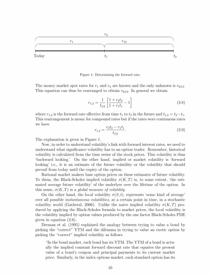
The answer is yes. This is done by fixing a forward rate. A forward rate ofinterest is the rate of interest, implicit in currently quoted spot rates, that would beapplicable from one time point in the future to another time point in the future (Brigo& Mercurio, 2001). In the market, a forward rate is quoted as 6X12 for instance.This points to a rate that is applicable in 6 months time and ends in 12 month’s time.A time line explanation is given in Fig. 2.

Forward rates are not usually quoted and has to be implied from spot rates throughan arbitrage argument. Let’s assume we want to invest an amount A for 12 months.There are two alternative ways we can do this:

• invest at the 12 month rate given by r2; or

• invest at the 6 month rate for 6 months given by r1. After 6 months, role theinvestment for another 6 months. There are risks in this due to us not knowingwhat the rates are going to be in 6 months time. So, let’s assume we can fixthis rate today and that we reinvest at the 6X12 forward rate given by r6|12.

Both investments mature at the same time. If there are no arbitrage opportunities,we should end up with the same amount of money. Thus (using simple rates)

A(1 + r1 × 0.5)(1 + r6|12 × 0.5) = A(1 + r2).

9

Today t1 t2

r1 r12

r2

Figure 1: Determining the forward rate.

The money market spot rates for r1 and r2 are known and the only unknown is r6|12.This equation can thus be rearranged to obtain r6|12. In general we obtain

r1,2 =1

t1|2

[1 + r2t21 + r1t1

− 1

](3.8)

where r1,2 is the forward rate effective from time t1 to t2 in the future and t1,2 = t2−t1.This rearrangement is messy for compound rates but if the rates were continuous rateswe have

r1,2 =r2t2 − r1t1

t1|2. (3.9)

The explanation is given in Figure 1.Now, in order to understand volatility’s link with forward interest rates, we need to

understand what significance volatility has to an option trader. Remember, historicalvolatility is calculated from the time series of the stock prices. This volatility is thus‘backward looking.’ On the other hand, implied or market volatility is ‘forwardlooking’ i.e., it is an estimate of the future volatility or the volatility that shouldprevail from today until the expiry of the option.

Rational market makers base option prices on these estimates of future volatility.To them, the Black-Scholes implied volatility σ(K,T ) is, to some extent, ‘the esti-mated average future volatility’ of the underlyer over the lifetime of the option. Inthis sense, σ(K,T ) is a global measure of volatility.

On the other hand, the local volatility σ(S, t), represents ‘some kind of average’over all possible instantaneous volatilities, at a certain point in time, in a stochasticvolatility world (Gatheral, 2006). Unlike the naive implied volatility σ(K,T ) pro-duced by applying the Black-Scholes formula to market prices, the local volatility isthe volatility implied by option values produced by the one factor Black-Scholes PDEgiven in εquation (2.6).

Derman et al. (1995) explained the analogy between trying to value a bond bypicking the “correct” YTM and the dilemma in trying to value an exotic option bypicking the “correct” implied volatility as follows

“In the bond market, each bond has its YTM. The YTM of a bond is actu-ally the implied constant forward discount rate that equates the presentvalue of a bond’s coupon and principal payments to its current marketprice. Similarly, in the index options market, each standard option has its

10

own implied volatility, which is the implied constant future local volatilitythat equates the Black-Scholes value of an option to its current marketprice.

They also stated this differently (Kani et al., 1996)

“The forward rate from one future time to another can be found from theprices of bonds maturing at those times (see Figure 2) similarly, the localvolatility at a future stock level and time is related to options expiring inthat neighborhood.”

This became obvious when Dupire (1993) and Derman & Kani (1994) noted,that, knowing all European option prices merely amounts to knowing the probabilitydensities of the underlying stock price at different times, conditional on its currentvalue. Further insight came when they realised that under risk neutrality, there was aunique diffusion process consistent with the risk neutral probability densities derivedfrom the prices of European options. This diffusion is unique for any particular stockprice and holds for all options on that stock, irrespective of their strike level or timeto expiration. Remember that under the general Black-Scholes theory, the impliedvolatility skew infers that one stock should have many different diffusion processes:one for every strike and time to expiry. This, of course, cannot be the case.

Kani et al. (1996) further showed that the local variance, σ2(K,T ) is the con-ditional risk-neutral expectation of the instantaneous future variance of the stockreturns, given that the stock’s level at the future time T is K. We can also interpretthis measure as a K-level, T -maturity forward-risk-adjusted measure. This is anal-ogous to the known relationship between the forward and future spot interest rateswhere the forward rate is the forward-risk-adjusted expectation of the instantaneousfuture spot rate (Brigo & Mercurio, 2001).

They carry on

“Implied trees (or local volatility models) take a similar approach to ex-otic options. They avoid implied volatility, and instead use the volatilitysurface of liquid standard options to deduce future local volatilities. Then,they use these local volatilities to value all exotic options.”

Dupire, Derman, Kani and Kamal rediscovered a known (but lost) theorem statedand proved a decade earlier. They proofed it independently from a practitioner’s pointof view. This was a proposition by Krylov but proven by Gyongy (1986). Gyongy’stheorem is an important theoretical result that links local volatility models to otherdiffusion models that are also capable of generating the implied volatility surface.

Alexander & Nogueira (2008) pointed out that the basic idea is that, a givenstochastic differential εquation (SDE) with stochastic drift and diffusion coefficients,can be mimicked by another constructed process. However, this mimicking SDEcan be constructed such that it has deterministic coefficients such that the solutionsof the two equations have the same marginal probability distributions. In essence,Gyongy’s theorem states that the local volatility SDE given in εquation (2.5) is just

11

a special case of a more general stochastic differential equation with stochastic driftand volatility.

With Gyongy one can map a multi-dimensional Ito process to a one-dimensionalMarkov process with the same marginal distributions as the original process. It isused by practitioners to construct simpler SDEs by, for instance, reducing the numberof stochastic processes in models that incorporate stochastic volatility and stochasticinterest rates and/or dividends. Read more on this important theorem in AppendixB.

3.3. What does it Mean in Practice?

We know that every option volatility that is traded in the market, is linked toa strike and a time as depicted by the implied volatility surface — we say tradedvolatility is state and space dependent. Conceptually, implied volatility representsthe average amount of movement that we expect the stock to experience given thatthe stock price is to reach its given strike at the given time of expiration T .

Further remember that volatility measures variability, or dispersion about a cen-tral tendency — it is simply a measure of the degree of price movement in a stock,futures contract or any other market. The implied volatility is the amount that themarket thinks the stock would change on average over a period of time. Practi-cally, under the Black-Scholes assumption of normality, a 10% annualised volatilityrepresents the following: in one year, returns will be within [-10%; +10%] with aprobability of 68.3% (1 standard deviation from the mean); within [-20%; +20%]with a probability of 95.4% (2 standard deviations), and within [-30%; +30%] with aprobability of 99.7% (3 standard deviations).

3.3.1. Implied and Instantaneous Volatility

In order to understand what is meant by “local” volatility, we need to refreshour memory on historical, implied and instantaneous volatilities. Gatheral (2006)stated that the local volatility is representing ‘some kind of average over all possibleinstantaneous volatilities ’ in a stochastic volatility world. This is confusing becausethe implied volatility seems to be defined in exactly the same way: implied volatilityis equal to the quadratic mean volatility from 0 to an expiry time T . What does thismean?

If market volatilities are not known, many traders will look at historical volatilities(also known as realised volatility). Let’s assume we have a stock price that diffusesthrough time. The prices are given by S1, S2, S3, . . . Si, . . . Sn and Si is the stock priceat the end of the i-th time interval where i = 1, 2, 3, . . . n. The logarithmic (perperiod) returns are defined as

xi = ln

(Si+1

Si

). (3.10)

12

The standard deviation is then given by

σ(T ) =

√∑ni=1 (xi − x)2

n, (3.11)

where x is the mean of all xi. σ(T ) in εquation (3.11) is defined as the historicalvolatility over the time interval [0, T ]. Note, this is the average volatility for our ndiscrete time intervals.

To enable us to compare volatilities for different interval lengths we usually expressvolatility in annual terms. To do this we scale this estimate with an annualisationfactor (normalising constant) which is the number of intervals per annum such that

σannual = σ(T )×√h.

If daily data is used the interval is one trading day, then we use h = 252 businessdays per annum, if the interval is a week, h = 52 and h = 12 for monthly data.Note, annualisation is just a simplification of a more complex theory and cannot beused with high frequency or intra-day tick data: limh→∞ σannual → ∞ explodes as hbecomes larger and larger.

An example is shown in Table 1 and Figure 2 for some stock with 11 prices and10 time intervals. If the time interval for our example was one day, then Table 1

Steps/ Price (Si) Logarithmic ForwardTime Returns (xi) Instantaneous

Volatility (σinst)1 100 9.9751%2 101 0.0099503 9.9259%3 102 0.0098523 9.9259%4 101 -0.0098523 20.1021%5 97 -0.0404095 10.1274%6 98 0.0102565 10.0759%7 99 0.0101524 17.2780%8 102 0.0298530 9.8773%9 103 0.0097562 14.0030%10 101 -0.0196085 9.9751%11 100 -0.0099503

StandardDeviation 2.00%AnnualisedHistoricalVolatility 31.77%

Table 1: Prices and volatilities for some stock.

shows that the annualised volatility (or realised volatility) for this discrete time series

13

is 31.77%. This is just the average of the per period volatility of 2% multiplied by√252. This might not make sense if we have daily or even monthly data. However,

these time intervals can be made as small as possible and in the limit as n→∞, wearrive at the true instantaneous volatility.

Figure 2: Price path of some stock showing the standard deviation, annualised volatility and instan-taneous volatilities.

Figure 2 shows the prices after each time interval. Also shown is the definitionof the instantaneous volatility which is just the square root of the logarithmic returnper period as given by εquation (3.10) or

σinst(ti) =√xi. (3.12)

Note that instantaneous volatility is time dependent only

This definition is similar to the definition for the instantaneous forward interestrate eluded to in Section (3.2) (Brigo & Mercurio, 2001). In the market the smallesttime interval might be one second and we can then calculate a ‘market instantaneousvolatility’ from one second to the next.

It is very important to note the way we calculate the forward instantaneous volatil-ity:

σinstant(t = 4) =√x4 =

√ln(S5/S4).

Furthermore, if we have a real historic time series of stock prices, we can only obtainone instantaneous volatility at each time step. In Table 1 we list the 10 forwardinstantaneous volatilities for the 11 given stock prices.

14

3.3.2. Local Volatility by Example

If we understand the concept of instantaneous volatility, we are much closer inunderstanding the statement by Gatheral (2006): local volatility is representing somekind of average over all possible instantaneous volatilities in a stochastic volatilityworld.

In Figure 2 we plotted one price path and from the previous section we now knowwe can estimate the forward instantaneous volatilities at each time step. However,instantaneous volatility is time dependent only, but we know that local volatility isstate and space dependent. Instantaneous volatility alone does not, unfortunately,bring us much closer to an explanation of local volatility. Local volatility can neverbe obtained from market or historical stock prices. It can only be obtained throughsimulation or from option prices in the market. We’ll discuss the algebraic mappingdue to Dupire (1994) in Section 3.5. Tree numerical schemes were discussed byDerman & Kani (1994) and Rubinstein (1994).

Let’s try to understand local volatility through simulation. In Figure 3 we show atypical price path of a stock as it starts at a price of R100 on 10 February 2014 and itdiffuses discretely through time — this is similar to our example in Figure 2. However,these prices are simulated through a Monte Carlo process, they are not real marketvalues. This process should be governed by the correct stochastic volatility PDE. Wecan obtain the forward instantaneous volatilities for each time step as explained inthe previous section. From this simulation we estimate the implied/realised volatilityover the 6 month period to be about 30%.

Figure 3: One simulated price path of some stock with a 30% volatility over a six month period

Let’s now run another simulation and add this price path to Figure 3. This isshown in Figure 4. We can now zoom in on 26 May 2014 where the stock price levelis R95. We note that for this particular example, the two simulated price paths cross

15

and both arrived at the same stock price at the same time. On this date, we havetwo price paths and we can thus calculate two forward instantaneous volatilities.

Figure 4: Two simulated price paths of some stock with a 30% volatility over a six month period

The local volatility is then defined, a la Gatheral, as the average of these twoinstantaneous volatilities. Why? Remember, we know that local volatility is stateand space dependent, thus the specific level of the stock price has to come into playas well. Crucial is the fact that we are at an instant of time at a certain stock price.

We can generalise the simulation by generating an infinite number of price pathsthrough simulation. Through the law of large numbers, we expect to have an infinitenumber of paths that will pass through the R95 level (Duffie, 1996). We can thencalculate the local volatility as follows

σ(R95, 26May2014) =

√√√√ 1

m

m∑j=1

xj,

where we have m (m → ∞) price paths running through R95 meaning we will havem instantaneous volatilities. In other words, the “local volatility is representing somekind of average over all possible instantaneous volatilities”.

We can now generalise this further if we realise that, if we run an infinite num-ber of simulations we will have many paths passing through every conceivable stockprice S on 26 May 2014 where S ∈ R+

0 . We will actually end up with many, manyprice paths passing through every stock price at every time interval. In practice weonly have discrete time intervals and also discrete stock prices, so we can state this

16

mathematically as follows

σ(Sk(ti), ti) =

√√√√ 1

m

m∑j=1

xj(Sk(ti), ti), (3.13)

where ti is the i-th time interval (i = 1, 2, 3, . . . , n) and Sk is the k-th price at time tiwhere k = 1, 2, 3, . . . , l such that we have l stock prices at each time interval.

If we do this numerically for a discrete number of stock prices and a discretenumber of time intervals, we end up with a matrix where we have a local volatilityfor every stock price at every time interval. In Figure 4 counter i runs from left toright across time and k from bottom to top across different stock prices. In the limitsas n,m, l→∞, we’ll end up with the continuous version.

In our example shown in Figure 4, we can do this for every possible future timefrom 10 February 2014 till 10 August 2014 and every possible price at each time. Ifwe do this we obtain the whole local volatility surface. In practise we can only do itdiscretely and thus we do it for every day, week or month. We can for instance dividethe time to expiry into monthly buckets and choose stock levels from R10 to R200 inincrements of R10. We then determine the local volatility for every price and everybucket giving us a grid of volatilities. Such a grid (matrix) is shown in Figure 5 and itrepresents the local volatility surface. From Figure 5 we deduce that, although localvolatilities are not “real”, they look similar to the market or implied volatilities.

3.3.3. Sticky Local Volatility

We now know that local volatility is the name given for the instantaneous volatilityof an underlying (i.e., the exact volatility), at a certain point in time at a specificstock level St. The volatility is “stuck” to the price of the underlying at that pointin time and we thus call such a surface a “sticky local volatility surface.” This can becompared to a sticky strike or a sticky delta implied volatility surface.

From Sections 3.2 and 3.3.1, we know that the Black-Scholes implied volatility ofan option with strike K is equal to the average (across time) local (or instantaneous)volatility of all possible paths of the underlying from spot at S0 to strike K. This canbe approximated by the average of the local volatility at spot and the local volatilityat strike K. Bennett & Gil (2012) shows that this approximation leads to threeresults:

• The ATM Black-Scholes volatility is equal to the ATM local volatility.

• The Black-Scholes skew is half the local volatility skew (due to averaging).Skew here is similar to the slope of the curve. In the market it is usually takenas, simply, the difference between the 90% strike volatility and 100% strikevolatility.

• A sticky local volatility surface implies a negative correlation between spot andimplied volatility — The local volatility framework is thus very realistic (Kotze& Joseph (2009) discusses this feature with examples).

17

Figure 5: A grid or matrix showing possible local volatilities per time bucket and price level.

The second point is understood through the following example:Let’s assume the local volatility for the 90% strike is 22% and the ATM local volatilityis 20%. The 90%-100% local volatility skew is therefore 2%. As the Black-Scholes90% strike option will have an implied volatility of 21% (the average of 22% and20%), it has a 90%-100% skew of 1% (as the ATM Black-Scholes volatility is equal tothe 20% ATM local volatility). This is half the local volatility skew. The dynamicsof the sticky local volatility surface is depicted in Figure 6.

Figure 6: Dynamics of a local volatility surface (Taken from Bennett & Gil (2012)).

18

3.4. Local Volatility by a Deterministic Volatility Function

Local volatility is not traded and thus is not a measurable quantity like impliedvolatility. Local volatility must be calculated somehow. This was a conundrum for along time. Practitioners and quants knew from the start that there should be somelink between the implied and local volatility. This makes sense because the impliedvolatility, σ(K,T ) is just a special case of the local volatility σ(S, t) such that

σ(K,T ) ∝ σ(S, t).

Remember that K,S ∈ R+0 and t ∈ [0, T ].

Before a derivative can be priced using the local volatility, we need to obtain thelocal volatility function. Before the mid-1990s, quants calculated the local volatilitysurface by pricing a vanilla option using the general Black-Scholes equation and theimplied volatility from the traded skew. The local volatility could then (and still can)be found by setting

Vl(σ(S, t))− Vbs(σ(K,T )) = 0

and then finding σ(S, t) by solving εquation (2.6) numerically by MC or FD methods.Optimisation is usually done by nonlinear least squares (NLS).

The local volatility surface obtained in this manner is in general not smooth.Dumas et al. (1998) realised that if volatility is a deterministic function of asset priceand/or time, option valuation based on the Black-Scholes partial differential equationin (2.6) remains possible, although not by means of the Black-Scholes formula itself.They stated this is a special case and termed it the “deterministic volatility function”(DVF) hypothesis. They further stated that the reliability of this hypothesis dependscritically on how well one can estimate the dynamics of the underlying asset pricefrom a cross section of option prices.

Carr et al. (2013) recently proved that a quadratic analytic functional form forthe local volatility is tractable in accordance to the local volatility SDE in εquation(2.5). This was previously empirically proven by Dumas et al. (1998).

3.5. Dupire Local Volatility

Let’s recap what we know: From εquation (2.5) we know that the general Black-Scholes differential equation is obtained from the SDE

dSt = (r − d)Stdt+ σ(St, t)StdWt. (3.14)

In its most general form, the function σ(S, t) is called the instantaneous volatilityfor an option with time to expiry T and its dynamics are stochastic. Furthermore,similar to the definition of the instantaneous forward interest rate (Brigo & Mercurio,2001), we define the implied volatility as follows

σ(K,T ) =

√1

T

∫ T

0

σ2(t)dt (3.15)

19

by additivity of variance (Clark, 2011). This shows that the implied volatility is afair average, across time, over all instantaneous variances.

Readers might be confused due to the last paragraph in Section 2.1 and εquation(2.4) where we stated that the implied volatility is not a volatility after all. Theinstantaneous volatility/variance in εquation (3.15) is not the true volatility of thestochastic process St. It is something different as explained in Section 3.

We further know that the Black-Scholes backward parabolic equation in variablesS and t, given in (2.6), is the Feynman-Kac representation of the discounted expectedvalue of the final option value as given in (2.7) (Cozzi, 2012).

Dupire (1993) attempted to answer the question of whether it was possible toconstruct a state-dependent instantaneous volatility that, when fed into the one-dimensional diffusion equation given in (3.14), will recover the entire implied volatilitysurface σ(K,T )? This suggests he wanted to know whether a deterministic volatilityfunction exists that satisfies εquation (3.14). The answer to this question is negative,however, it becomes true if we apply Gyongy’s theorem where the stochastic differ-ential equation in (3.14) is transformed to another SDE with a non-random volatilityfunction. This is ultimately what Dupire (1994) proved.

According to standard financial theory, the price at time t of a call option withstrike price K, maturity time T is the discounted expectation of its payoff, underthe risk-neutral measure. Dupire (1994) assumed that the probability density of theunderlying asset St at the time t has to satisfy the forward Fokker-Planck εquation(also known as the forward Kolmogorov equation) given by

∂

∂tϕ =

1

2

∂2

∂S2T

(σ2(ST , T )S2Tϕ)− St

∂

∂ST((r − d)STϕ) (3.16)

where ϕ ≡ ϕ(ST , T ) is the forward transition probability density of the random vari-able ST (final S at expiry time T ) in the SDE shown in εquation (3.14) (Clark, 2011).However, using the the Breeden-Litzenberger formula (Breeden & Litzenberger, 1978)

∂2C

∂K2= ϕ(K,T ), (3.17)

and doing a bit of calculus (see Clark (2011) and Gatheral (2006)), we can rewritethis and obtain the Dupire forward equation in terms of call option prices C(K,T )[

∂

∂T+ (r − d)K

∂

∂K− 1

2σ2(K,T )K2 ∂2

∂K2+ d

]C(K,T ) = 0 (3.18)

where σ(K,T ) is continuous, twice-differentiable in strike and once in time, and localvolatility is uniquely determined by the surface of call option prices. Note how, whenmoving from the backward Kolmogorov εquation (the Black-Scholes PDE given in(2.3)) to the forward Fokker-Planck equation, the time to maturity T has replacedthe calendar time t and the strike K has replaced the stock level S. The Fokker-Planck equation describes how a price propagates forward in time. This equationis usually used when one knows the distribution density at an earlier time, and one

20

wants to discover how this density spreads out as time progresses, given the drift andvolatility of the process (Rebonato, 2004). Dupire’s forward equation also providesuseful insights into the inverse problem of calibrating diffusion models to observedcall and put option prices.

This forward PDE is very useful because it holds in a more general context thanthe backward PDE: even if the (risk-neutral) dynamics of the underlying asset is notnecessarily Markovian, but described by a continuous Brownian martingale

dSt = StσdWt

then call options still verify a forward PDE where the diffusion coefficient is given bythe local (or effective) volatility function σ(S, t) given by

σ(S, t) =√E[σ2|St = S]

and σ is the instantaneous or stochastic volatility of the process St. This method islinked to the Markovian projection problem: the construction of a Markov processwhich mimics the marginal distributions of a martingale. Such mimicking processesprovide a method to extend the Dupire equation to non-Markovian settings (seeAppendix B).

Dupire (1994) used the strike/dual Gamma (∂2C/∂K2) of a call option, that givesthe marginal probability distribution function (Breeden & Litzenberger, 1978), andthought of this as timeslices of the forward transition probabilities. Now, since theforward Fokker-Planck equation in εquation (3.16) describes the time evolution offorward transition probabilities, we can isolate the volatility coefficients that recoverthe prices of tradable call options for all strikes and all times in εquation (3.18).

Dupire actually proved that it is possible to find the same option price solving adual problem, namely a forward parabolic equation in the variables K and T knownas the dual Black-Scholes equation or Dupire’s equation. This equation is actually theFokker-Planck equation for the probability density function of the underlying assetintegrated twice. This solution allows us to calculate the price of an European calloption for every strike and maturity, given the present spot value S and time t.

Dupire (1994) solved for the volatility and got

σ2loc(K,T ) = 2

∂C(K,T )

∂T+ C(K,T )d+ (r − d)K ∂C(K,T )

∂K

K2 ∂2C(K,T )∂K2

. (3.19)

Thus, given prices for all plain-vanilla call options C(K,T ) today, σloc(K,T ) is thelocal volatility that will prevail at time T (t = T ) when the future stock price is equalto K (ST = K). We refer the reader to Appendix A.1 for a full derivation of εquation(3.19). Note that r is a fixed interest rate and d a fixed dividend yield, both incontinuous format. See the number 2 on the right hand side of εquation (3.19). Thisbacks our statement in Section 3.3.3 up where we stated that the implied volatility ishalf the local volatility skew.

21

εquation (3.19) ensures the existence and uniqueness of a local volatility surfacewhich reproduces the market prices exactly

We further note that for εquation (3.19) to make sense, the right hand side must bepositive. How can we be sure that volatilities are not imaginary? This is guaranteedby no-arbitrage arguments. We have from the denominator

σ2loc(K,T ) ∝

(K2 × ∂2C

∂K2

)−1.

K2 is positive always and, the dual gamma or risk-neutral price density must bepositive in the absence of arbitrage (butterfly spread). To ensure the positivity of thenumerator, we note that no-arbitrage arguments state that calendar spreads shouldhave positive values. Kotze & Joseph (2009) and Kotze et al. (2013) discusses no-arbitrage arguments in detail.

An implied volatility surface is arbitrage free if the local volatility is a positivereal number (not imaginary) where σloc(K,T ) ∈ R+

0

Since, at any point in time, the value of call options with different strikes andtimes to maturity can be observed in the market, the local volatility is a deterministicfunction, even when the dynamics of the spot volatility is stochastic — Gyongy. Also,εquation (3.19) is conceptually equivalent to the Derman & Kani (1994) tree approach.

Dupire’s εquation (3.19) is not analytically solvable. The option price function(and the derivatives) in this equation have to be approximated numerically. Thederivatives are easily obtained in using Newton’s difference quotient. To obtain thedual delta, ∂C/∂K, we therefore use

∂C(K,T )

∂K=C(K + ∆K, σ(K + ∆K,T ))− C(K, σ(K,T ))

∆K(3.20)

where we note that all calls should be priced with the implied volatility smile. Here,C(K + ∆K, σ(K + ∆K,T )) denotes a call price at a strike of K + ∆K where theimplied volatility is found from the implied volatility skew for this option expiring atT with a strike of K + ∆K. To find an optimal size of the bump, ∆K, it should betested for. For an index like the Top 40, one or ten index points works very well butsome people prefer it to be a percentage of the strike price. Beware not to make ittoo big — 1% might seem small but it is in general too big. One or 10 basis pointsworks rather well for the time bump.

Beware, one cannot use the closed-form Black-Scholes derivatives for the dualdelta. We call the numeric dual delta in εquation (3.20), the impact/modified dualdelta. Traders call the ordinary delta calculated this way, i.e., with the skew, theimpact/modified delta due to the fact that it gives a truer reflection (or impact) of

22

the dynamic hedging process — it takes some of the nonlinear effects of the Black-Scholes equation, together with the shape of the volatility skew, into account. Thedual gamma is numerically obtained by

∂2C(K,T )

∂K2=C(K + ∆K, σ(K + ∆K))− C(K −∆K, σ(K −∆K))− 2C(K, σ(K))

∆K2

where we dropped the T for clarity sake. Rebonato (2004) gives a full discussion onfinding these derivatives numerically.

Solving εquation (3.19) numerically has its own issues. Problems can arise whenthe values to be approximated are very small and small absolute errors in the approx-imation can lead to big relative errors, perturbing the estimated quantity heavily.Determining the density is numerically delicate. It is very small for options that arefar in- or out-of-the-money (the effect is particularly large for options with short ma-turities). Small errors in the approximation of this derivative will get multiplied bythe strike value squared resulting in big errors at these values, sometimes even givingnegative values, resulting in negative variances and complex local volatilities. Thelocal volatility will remain finite and well-behaved only if the numerator approacheszero at the right speed for these cases.

Further to the numerical issues, the continuity assumption of option prices is, ofcourse, not very realistic. In practice option prices are known for certain discretepoints and at limited number of maturities (quarterly for instance like most Safexoptions). The result of this is that in practice the inversion problem is ill-posed i.e.the solution is not unique and is unstable — the positivity of the second derivativein the strike direction is not guaranteed.

3.6. Local Volatility in terms of Implied Volatility

The instability of εquation (3.19) forces us to consider alternatives. We knowoptions are traded in the market on implied volatility and not price. Can we thus nottransform this equation such that we supply the implied volatilities instead of optionprices?

This can be done if a change of variables is made in (3.19) by rewriting the Black-Scholes equation for a call C in terms of the log-strike y where y = log(strike/Forward).This leads to (Wilmott (1998) and Clark (2011))

σ2loc(K, τ) =

σ2imp + 2τσimp

∂σimp∂τ

+ 2(r − d)Kτσimp∂σimp∂K(

1 +Kd1√τ∂σimp∂K

)2

+K2τσimp

(∂2σimp∂K2 − d1

√τ

(∂σimp∂K

)2) ,(3.21)

where

d1 =ln (S0/K) +

((r − d) + σ2

imp/2)τ

σimp√τ

,

and τ = T − t such that t and S0 are respectively the market date, on which thevolatility smile is observed, and the asset price on that date. Note that εquation

23

(3.21) gives the variance, i.e., σ2. See Appendix A.2 for the derivation.When comparing εquation (3.19) with (3.21) it is clear that the problem of nu-

merical large errors no longer exists. The transformation of Dupire’s formula into onewhich depends on the implied volatility ensures that the dual Gamma is no longeralone in the denominator as it was in (3.19). The second derivative of the impliedvolatility is now one term of a summation, so small errors in it will not necessarilylead to large errors in the local volatility function. However, small differences in theinput volatility surface can produce a big difference in the estimated local volatility.

The main problem is that the implied or traded volatilities are only known atdiscrete strikes K and expiries T . This is why the parameterisation chosen for theimplied volatility surface is very important. If implied volatilities are used directlyfrom the market, the derivatives in εquation (3.21) needs to be obtained numericallyusing finite difference or other well-known techniques. This can still lead to an unsta-ble local volatility surface. Furthermore we will have to interpolate and extrapolatethe given data points unto a surface. Since obtaining the local volatility from thedata involves taking derivatives, the extrapolated implied volatility surface cannot betoo uneven. If it is, this unevenness will be exacerbated in the local volatility surfaceshowing that it is not arbitrage free in these areas.

In the foreign exchange market, options are traded on the Delta — effectively ameasure of the moneyness — as opposed to the absolute level of the strike. SeeClark (2011) for the FX version of εquation (3.21)

4. The ALSI: Exact Implementation

4.1. The Deterministic Implied Volatility Function

The issues relating to determining the derivatives in εquation (3.21) are circum-vented in two ways:

• Choose a particular functional form for the implied volatility surface and fit thisfunction to the market volatility data.

• Choose a particular functional form for the local volatility surface and find itusing non-linear optimisation techniques.

This is the route Safex took for the liquid ALSI options. Safex uses the followingthree parameter deterministic quadratic function as a good model of fit for the ALSIimplied volatility data on every expiry date (for a full discussion see Kotze & Joseph(2009) and Kotze et al. (2013))

σmodel(β0, β1, β2, Tk) = βk0 + βk1 M + βk2 M2. (4.22)

Tk are the times to expiry for all listed expiry dates such that k = 1, 2, . . . , n and nis the total number of listed expiries. This equation, of course, describes a parabola(for each expiry) and this conic section has the following properties (loosing thesuperscript k)

24

• M = S/K is the strike price in moneyness format (Spot/Strike),

• β0 is the constant volatility (shift or trend or level) parameter, β0 > 0. Notethat

σ → β0M→0

.

This means that β0 is similar to the Y -intercept for a parabola. We have, in theCartesian plane, the Y -axis being σmodel and the X-axis being the moneyness.

• β1 is the correlation (slope) term. This parameter accounts for the negative cor-relation between the underlying index and volatility. The no-spread-arbitragecondition requires that −1 < β1 < 0.

• β2 is the volatility of volatility (‘vol of vol’ or curvature/convexity) parameter.The no-calendar-spread arbitrage convexity condition requires that β2 > 0.

Note that εquation (4.22) is linear in the wings if M → ±∞ and it holds for discreteexpiry time T . These properties and constraints are the factors describing the shapeof the skews — they are not the no-arbitrage constraints. They are, however, relatedto the no-arbitrage conditions imposed on a volatility skew and surface — these arediscussed in Kotze et al. (2013).

The n parabolas described by εquation (4.22) can now be fitted to the relevantoption data (obtained per expiry date) independently to give us n discrete skews. Inorder to incorporate the time dependence and generate a continuous smooth impliedvolatility surface we also need a specification or functional form for the at-the-money(ATM) volatility term structure. It is, however, important to remember that theATM volatility is intricately part of the skew. This infers that the two optimisations(one for the skews and the other for the ATM volatilities) can not be done stricklyseparate from one another. Taking the ATM term structure together with each skewwill give us the 3D implied volatility surface.

It is well-known that volatility is mean reverting; when volatility is high (low) thevolatility term structure is downward (upward) sloping Gatheral (2006). Safex usesthe following exponential functional form for the ATM volatility term structure

σatm(M, t) =θ

tλ. (4.23)

Here we have (See Kotze & Joseph (2009) for full details)

• t is the time to expiry,

• λ controls the overall slope of the ATM term structure; λ > 0 implies a down-ward sloping ATM volatility term structure, whilst a λ < 0 implies an upwardsloping ATM volatility term structure, and

• θ controls the short term ATM curvature.

25

We now assume that each of the parameters β in εquation (4.22) must adhere toεquation (4.23) such that

βi(t) =θitλi

; i = 0, 1, 2. (4.24)

To ensure the surface is continuous we dropped the superscript k and changed thediscrete expiry times Tk to a continuous time t where Tk ∈ t; t ∈ R+

0 . CombiningEquations (4.22) and (4.24) leads to

σimp(M, t) =θ0tλ0

+θ1tλ1M +

θ2tλ2M2. (4.25)

εquation (4.25) fully describes the 3D implied volatility surface. We have to find 6parameters by fitting this function to the market volatility skews using optimisationtechniques. From εquation (4.23) we know that λ controls the slope of the curves (wealso call this the scaling parameters) while θ controls the curvature. From εquation(4.22) we thus have

• β0 and λ0 are called the level or shift or trend parameters and they control thelevel of the volatility.

• β1 and λ1 are called the rho or tilt parameters and they control the overall slopeof the curves.

• β2 and λ2 are the volatility of volatility parameters and they control the curva-ture.

Kotze & Joseph (2009) mentions they use a floating surface such that MATM = 1i.e. the ATM strike is one. A floating surface is defined such that

σimp(M, t) = σATM(t) + σfloatimp (M, t) (4.26)

where σATM(t) is the market at-the-money volatility.Now, from εquation (4.25) we have

σATMimp (t) =θ0tλ0

+θ1tλ1

+θ2tλ2. (4.27)

Thus, combining εquations (4.25), (4.26) and (4.27) leads us to the final 3 dimensionalmarket volatility surface given by (transforming back from moneyness to the realworld i.e. substituting M = K/S)

σimp(S,K, t) = σATM(t) +θ1tλ1

(K

S− 1

)+θ2tλ2

((K

S

)2

− 1

). (4.28)

Safex obtains the ATM volatilities from the market meaning σATM(t) is a constantfor every t.

26

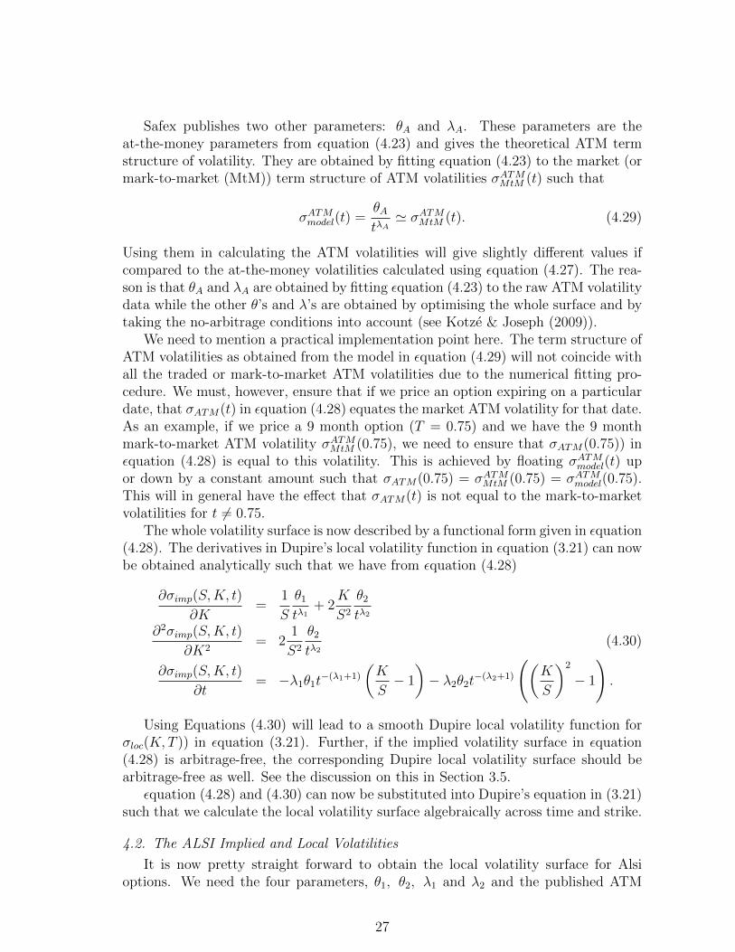
Safex publishes two other parameters: θA and λA. These parameters are theat-the-money parameters from εquation (4.23) and gives the theoretical ATM termstructure of volatility. They are obtained by fitting εquation (4.23) to the market (ormark-to-market (MtM)) term structure of ATM volatilities σATMMtM (t) such that

σATMmodel(t) =θAtλA' σATMMtM (t). (4.29)

Using them in calculating the ATM volatilities will give slightly different values ifcompared to the at-the-money volatilities calculated using εquation (4.27). The rea-son is that θA and λA are obtained by fitting εquation (4.23) to the raw ATM volatilitydata while the other θ’s and λ’s are obtained by optimising the whole surface and bytaking the no-arbitrage conditions into account (see Kotze & Joseph (2009)).

We need to mention a practical implementation point here. The term structure ofATM volatilities as obtained from the model in εquation (4.29) will not coincide withall the traded or mark-to-market ATM volatilities due to the numerical fitting pro-cedure. We must, however, ensure that if we price an option expiring on a particulardate, that σATM(t) in εquation (4.28) equates the market ATM volatility for that date.As an example, if we price a 9 month option (T = 0.75) and we have the 9 monthmark-to-market ATM volatility σATMMtM (0.75), we need to ensure that σATM(0.75)) inεquation (4.28) is equal to this volatility. This is achieved by floating σATMmodel(t) upor down by a constant amount such that σATM(0.75) = σATMMtM (0.75) = σATMmodel(0.75).This will in general have the effect that σATM(t) is not equal to the mark-to-marketvolatilities for t 6= 0.75.

The whole volatility surface is now described by a functional form given in εquation(4.28). The derivatives in Dupire’s local volatility function in εquation (3.21) can nowbe obtained analytically such that we have from εquation (4.28)

∂σimp(S,K, t)

∂K=

1

S

θ1tλ1

+ 2K

S2

θ2tλ2

∂2σimp(S,K, t)

∂K2= 2

1

S2

θ2tλ2

(4.30)

∂σimp(S,K, t)

∂t= −λ1θ1t−(λ1+1)

(K

S− 1

)− λ2θ2t−(λ2+1)

((K

S

)2

− 1

).

Using Equations (4.30) will lead to a smooth Dupire local volatility function forσloc(K,T )) in εquation (3.21). Further, if the implied volatility surface in εquation(4.28) is arbitrage-free, the corresponding Dupire local volatility surface should bearbitrage-free as well. See the discussion on this in Section 3.5.

εquation (4.28) and (4.30) can now be substituted into Dupire’s equation in (3.21)such that we calculate the local volatility surface algebraically across time and strike.

4.2. The ALSI Implied and Local Volatilities

It is now pretty straight forward to obtain the local volatility surface for Alsioptions. We need the four parameters, θ1, θ2, λ1 and λ2 and the published ATM

27

volatilities. These parameters are published every two weeks when Safex updatestheir volatility surfaces.

In Table 2 we show the parameter values, θi and λi, (i = 1, 2, 3, ATM) as publishedby Safex on 28 May 2014. Also shown are the values for θi/t

λi , i = 0, 1, 2, 3. Table3 lists σATMimp , the model ATM volatilities and official Safex ATM volatilities for allexpiry dates. In Figure 7 we show the Alsi implied and corresponding local volatilitysurfaces.

CurvatureRho(θ1) VolVol (θ2) Level (θ0) Atm (θATM)

In Months -0.8488985 0.1945430 0.9139862 0.1350075In Years -0.4337514 0.1069264 0.4753064 0.1595808

DecayRho (λ1) VolVol (λ2) Level (λ0) Atm (λATM)0.2702186 0.2408592 0.2631310 -0.0672942

Date T θ1/tλ1 θ2/t

λ2 θ0/tλ1

19-06-2014 0.06027397 -92.655786% 21.033029% 99.531201%18-09-2014 0.30958904 -59.544292% 14.181881% 64.708854%18-12-2014 0.55890411 -50.759237% 12.301016% 55.393271%19-03-2015 0.80821918 -45.943944% 11.255306% 50.269616%18-06-2015 1.05753425 -42.724414% 10.549535% 46.836131%17-09-2015 1.30684932 -40.349172% 10.025150% 44.298712%15-12-2016 2.55342466 -33.668883% 8.531503% 37.140432%21-12-2017 3.56986301 -30.754183% 7.869980% 34.005870%

Table 2: Optimised parameters for the Alsi deterministic implied volatility function on 28 May 2014(see Equations (4.26), (4.27) and (4.28)).

Expiry Date Expiry Time Model ATM Safex ATMT σATMmodel(t) σATMMtM (t)

19-06-2014 0.06027397 13.209622% 14.2518-09-2014 0.30958904 14.747329% 14.0018-12-2014 0.55890411 15.345386% 14.5019-03-2015 0.80821918 15.731053% 15.0018-06-2015 1.05753425 16.018262% 15.7517-09-2015 1.30684932 16.248072% 16.7515-12-2016 2.55342466 16.997206% 18.5021-12-2017 3.56986301 17.384842% 21.00

Table 3: Model and official Safex ATM volatilities on 28 May 2014.

Continuing with our example in the previous section: if we want to price an

28

18 Dec 2014 Alsi option, we’ll have to float the model ATMs down by 0.15345386-0.145=0.00845386.

Figure 7: ALSI implied and local volatility surfaces on 28 May 2014

From Figure 7 we notice that the implied volatility surface does not have a lotof curvature — it is skewed but flat. However, we also see from the local volatilitysurface that it has more curvature. This shows that the local volatility skew is twicethat of the implied volatility as stated in Section 3.3.3.

5. Numerical Implementation of Dupire

In Section 4.1 we described the methodology implemented for obtaining the Alsivolatility surface and how the Dupire local volatility surface can be calculated al-gebraically. Unfortunately, such deterministic functions for the implied volatilitysurfaces for some of the other instruments like the DTOP (FTSE/JSE ShareholdersWeighted Top 40 Index) and USDZAR (US Dollar and South African Rand exchangerate), do not exist. The implied volatility surfaces are, however, available, albeitin a discrete form. All derivatives in εquation (3.21) have to be computed numeri-cally. The procedures and methodologies implemented at the JSE are discussed inthis section.

5.1. Volatility Interpolation and Extrapolation

In practice, we are often confronted with situations where only limited amount ofdata is accessible and it is necessary to estimate values between two consecutive givendata points. We can construct new points between known data points by interpolationor smoothing techniques.

All volatility surfaces of all derivatives listed on the JSE are available online.The following web sites should be visited:Equity indexes: https://www.jse.co.za/downloadable-files?RequestNode=

/Safex/mtmdata/VolSkewIndices

29

Single stock futures: https://www.jse.co.za/downloadable-files?

RequestNode=/Safex/mtmdata/VolSkewSSF

Bonds: https://www.jse.co.za/downloadable-files?RequestNode=

/YieldX/IRD_Vol_Skews

Only a handful of discrete points are given. The volatility surface (first 4 expiries)for the DTOP as published on 28 May 2014 is shown in Figure 8.

Figure 8: DTOP volatility surface as published by the JSE on 28 May 2014.

Inter- and extrapolation is thus necessary. At the JSE, we take the volatilities,square them and do linear inter- and extrapolation on the variance. However, it is atwo-dimensional problem. We have to do this across strike and across time. If youjust need to interpolate across strike prices use the following

σ2(K) = σ21 + (σ2

2 − σ21)K −K1

K2 −K1

.

Here we want to find the variance for a certain strike given by K where K1 ≤ K ≤ K2

and the volatility at K1 is σ1 and that at K2 is σ2. Further, σ21 ≤ σ2 ≤ σ2

2.When we interpolate across time only, we use what is known as flat forward inter-

polation. Volatility is time dependent. Suppose thatN time points t0 = 0, t1, t2, . . . , tNare given, and the implied volatilities for each of these time points are σ1, σ2, . . . , σN .We now define a general interpolation scheme to find the volatility at any time pointt where t ∈ R+

0 such that (Clark, 2011)

σ(t) =

σ1, t < t1√

1

t

[σ2i ti + σ2

i,i+1(t− ti)], ti ≤ t < ti+1 for i < N

σN , t ≥ tN

(5.31)

where

σ2i,i+1 =

σ2i+1ti+1 − σ2

i titi+1 − ti

.

30

5.2. Safex’s Implementation

We use the following 3 steps when we want to implement Dupire’s equation in(3.21) for all instruments except the ALSI

1. Read in the implied volatility surface as published by the JSE and convert it toa floating and moneyness format;

2. Regularise the surface, meaning we interpolate and plot it with more than thegiven 9 strikes per expiry;

3. Use this regularised implied volatility surface when we transform it to the localvolatility surface.

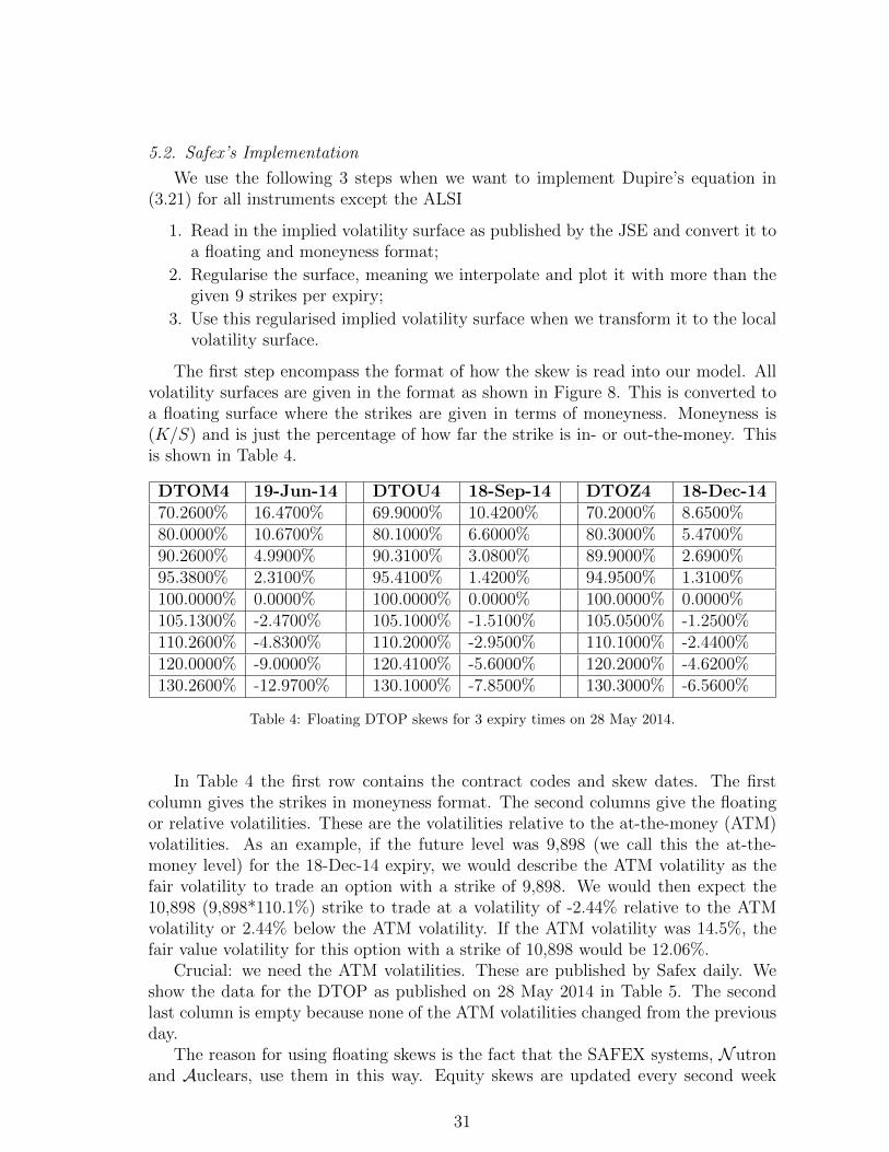
The first step encompass the format of how the skew is read into our model. Allvolatility surfaces are given in the format as shown in Figure 8. This is converted toa floating surface where the strikes are given in terms of moneyness. Moneyness is(K/S) and is just the percentage of how far the strike is in- or out-the-money. Thisis shown in Table 4.

DTOM4 19-Jun-14 DTOU4 18-Sep-14 DTOZ4 18-Dec-1470.2600% 16.4700% 69.9000% 10.4200% 70.2000% 8.6500%80.0000% 10.6700% 80.1000% 6.6000% 80.3000% 5.4700%90.2600% 4.9900% 90.3100% 3.0800% 89.9000% 2.6900%95.3800% 2.3100% 95.4100% 1.4200% 94.9500% 1.3100%100.0000% 0.0000% 100.0000% 0.0000% 100.0000% 0.0000%105.1300% -2.4700% 105.1000% -1.5100% 105.0500% -1.2500%110.2600% -4.8300% 110.2000% -2.9500% 110.1000% -2.4400%120.0000% -9.0000% 120.4100% -5.6000% 120.2000% -4.6200%130.2600% -12.9700% 130.1000% -7.8500% 130.3000% -6.5600%

Table 4: Floating DTOP skews for 3 expiry times on 28 May 2014.

In Table 4 the first row contains the contract codes and skew dates. The firstcolumn gives the strikes in moneyness format. The second columns give the floatingor relative volatilities. These are the volatilities relative to the at-the-money (ATM)volatilities. As an example, if the future level was 9,898 (we call this the at-the-money level) for the 18-Dec-14 expiry, we would describe the ATM volatility as thefair volatility to trade an option with a strike of 9,898. We would then expect the10,898 (9,898*110.1%) strike to trade at a volatility of -2.44% relative to the ATMvolatility or 2.44% below the ATM volatility. If the ATM volatility was 14.5%, thefair value volatility for this option with a strike of 10,898 would be 12.06%.

Crucial: we need the ATM volatilities. These are published by Safex daily. Weshow the data for the DTOP as published on 28 May 2014 in Table 5. The secondlast column is empty because none of the ATM volatilities changed from the previousday.

The reason for using floating skews is the fact that the SAFEX systems, Nutronand Auclears, use them in this way. Equity skews are updated every second week

31

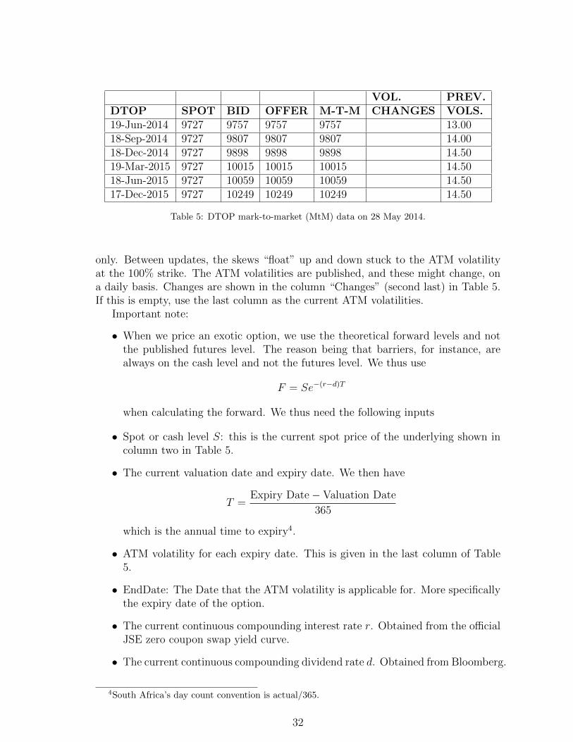
VOL. PREV.DTOP SPOT BID OFFER M-T-M CHANGES VOLS.19-Jun-2014 9727 9757 9757 9757 13.0018-Sep-2014 9727 9807 9807 9807 14.0018-Dec-2014 9727 9898 9898 9898 14.5019-Mar-2015 9727 10015 10015 10015 14.5018-Jun-2015 9727 10059 10059 10059 14.5017-Dec-2015 9727 10249 10249 10249 14.50

Table 5: DTOP mark-to-market (MtM) data on 28 May 2014.

only. Between updates, the skews “float” up and down stuck to the ATM volatilityat the 100% strike. The ATM volatilities are published, and these might change, ona daily basis. Changes are shown in the column “Changes” (second last) in Table 5.If this is empty, use the last column as the current ATM volatilities.

Important note:

• When we price an exotic option, we use the theoretical forward levels and notthe published futures level. The reason being that barriers, for instance, arealways on the cash level and not the futures level. We thus use

F = Se−(r−d)T

when calculating the forward. We thus need the following inputs

• Spot or cash level S: this is the current spot price of the underlying shown incolumn two in Table 5.

• The current valuation date and expiry date. We then have

T =Expiry Date− Valuation Date

365

which is the annual time to expiry4.

• ATM volatility for each expiry date. This is given in the last column of Table5.

• EndDate: The Date that the ATM volatility is applicable for. More specificallythe expiry date of the option.

• The current continuous compounding interest rate r. Obtained from the officialJSE zero coupon swap yield curve.

• The current continuous compounding dividend rate d. Obtained from Bloomberg.

4South Africa’s day count convention is actual/365.

32

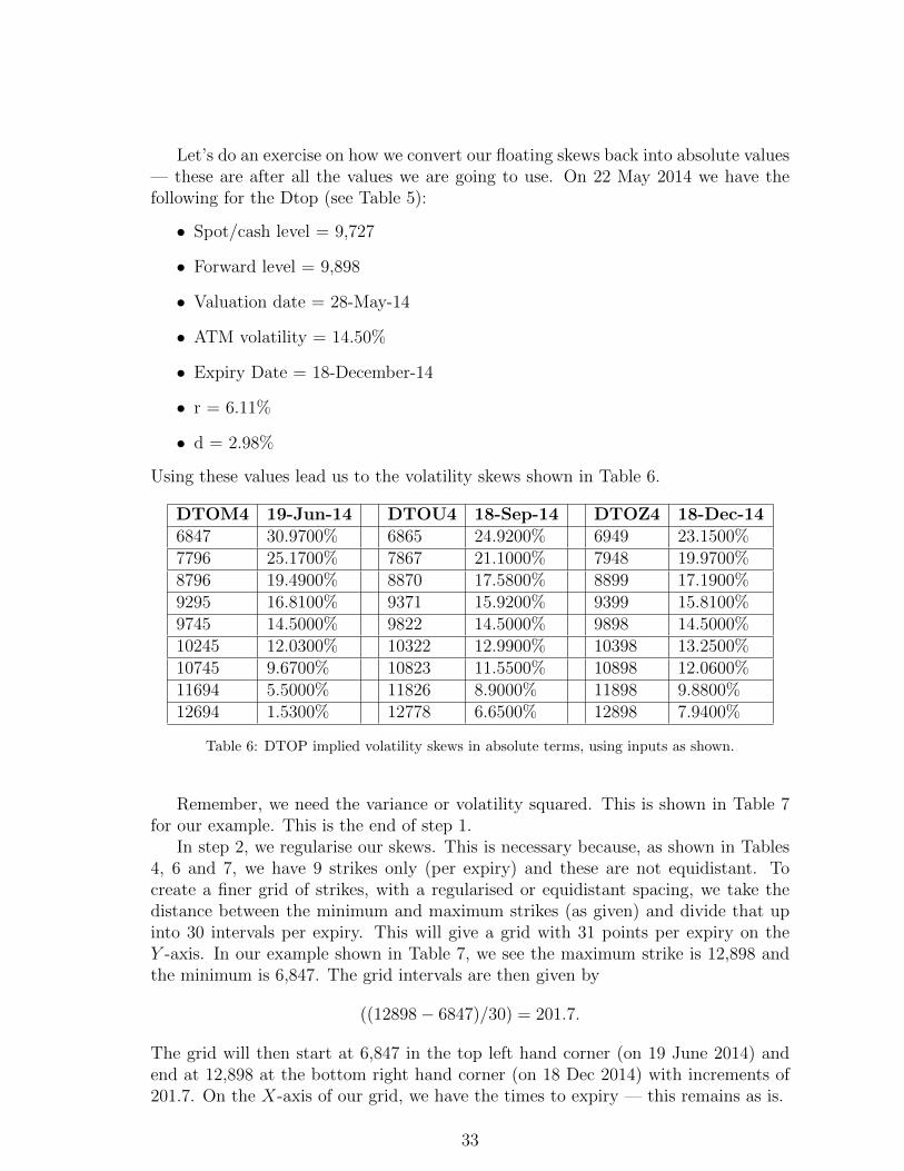
Let’s do an exercise on how we convert our floating skews back into absolute values— these are after all the values we are going to use. On 22 May 2014 we have thefollowing for the Dtop (see Table 5):

• Spot/cash level = 9,727

• Forward level = 9,898

• Valuation date = 28-May-14

• ATM volatility = 14.50%

• Expiry Date = 18-December-14

• r = 6.11%

• d = 2.98%

Using these values lead us to the volatility skews shown in Table 6.

DTOM4 19-Jun-14 DTOU4 18-Sep-14 DTOZ4 18-Dec-146847 30.9700% 6865 24.9200% 6949 23.1500%7796 25.1700% 7867 21.1000% 7948 19.9700%8796 19.4900% 8870 17.5800% 8899 17.1900%9295 16.8100% 9371 15.9200% 9399 15.8100%9745 14.5000% 9822 14.5000% 9898 14.5000%10245 12.0300% 10322 12.9900% 10398 13.2500%10745 9.6700% 10823 11.5500% 10898 12.0600%11694 5.5000% 11826 8.9000% 11898 9.8800%12694 1.5300% 12778 6.6500% 12898 7.9400%

Table 6: DTOP implied volatility skews in absolute terms, using inputs as shown.

Remember, we need the variance or volatility squared. This is shown in Table 7for our example. This is the end of step 1.

In step 2, we regularise our skews. This is necessary because, as shown in Tables4, 6 and 7, we have 9 strikes only (per expiry) and these are not equidistant. Tocreate a finer grid of strikes, with a regularised or equidistant spacing, we take thedistance between the minimum and maximum strikes (as given) and divide that upinto 30 intervals per expiry. This will give a grid with 31 points per expiry on theY -axis. In our example shown in Table 7, we see the maximum strike is 12,898 andthe minimum is 6,847. The grid intervals are then given by

((12898− 6847)/30) = 201.7.

The grid will then start at 6,847 in the top left hand corner (on 19 June 2014) andend at 12,898 at the bottom right hand corner (on 18 Dec 2014) with increments of201.7. On the X-axis of our grid, we have the times to expiry — this remains as is.

33

DTOM4 19-Jun-14 DTOU4 18-Sep-14 DTOZ4 18-Dec-146847 9.5914% 6865 6.2101% 6949 5.3592%7796 6.3353% 7867 4.4521% 7948 3.9880%8796 3.7986% 8870 3.0906% 8899 2.9550%9295 2.8258% 9371 2.5345% 9399 2.4996%9745 2.1025% 9822 2.1025% 9898 2.1025%10245 1.4472% 10322 1.6874% 10398 1.7556%10745 0.9351% 10823 1.3340% 10898 1.4544%11694 0.3025% 11826 0.7921% 11898 0.9761%12694 0.0234% 12778 0.4422% 12898 0.6304%

Table 7: Dtop variance skews. Volatilities from Table 6 converted

Next, we need the corresponding volatilities at each grid point. This is obtainedthrough inter- and extrapolation. In practice we use Matlab’s standard “interp1”function to interpolate and extrapolate the variance linearly for each respective time.The standard formula for this method is given in εquation (5.1).

As a final precaution we test all data points to ensure we never have volatilitiesabove 100% or below 1% — we clamp our volatilities to lie between these points.This grid forms the base for all further calculations. Finally, to enable us to dotemporal interpolation we convert the relative variance (being relative to time) into atotal variance, simply by multiplying the variance by the relevant time in years fromstart date. Why do we do this? Remember from the Black-Scholes equation that thevolatility is scaled by time through the factors σ

√(T ) and σ2T . This is the end of

step 2.The third and final step entails the implementation of Dupire’s formula in εquation

(3.21). At this point we note that the given strike and expiry time might still notfall on any given grid point. This is especially the case when we calculate the partialderivatives numerically. For such cases we make use of “bilinear interpolation5” onthe grid to arrive at a total variance for the given strike and time. This method firstinterpolates linearly on the Y -axis (strike) using εquation (5.1) and then uses thesame formula to interpolate on the X-axis (time). All values are then converted froma total variance (scaled by time) to an unscaled variance by dividing by time. Thesenumbers are tested for our allowable variance range where 0.01 ≤ σ2 ≤ 1, and arethen converted back to volatility.

When the derivatives in εquation (3.21) need to be calculated numerically, we useNewton’s difference quotient or finite difference formula. Differentiation with respectto time is implemented where we bump the time up by 1 basis point. We thus use

∂σ

∂t≈ f(t× (1− h))− f(t)

t× h.

5http://en.wikipedia.org/wiki/Bilinear_interpolation

34

When we differentiate with strike (dual Delta) we use a two-sided estimation where

∂σ

∂K≈ f(K × (1 + h))− f(K × (1− h))

K × (2h);

and the dual Gamma is given by

∂2σ

∂K2≈ f(K × (1 + h))− 2f(K) + f(K × (1− h))

(K × h)2.

The optimal h is found by using different h values and looking for stability. h isusually 1, 10, 25, 50 or 100 basis points.

5.3. Comparing the Implied and Local Volatilities for Dtop and Usdzar

Let’s be practical and look at the volatility surfaces for the Dtop and USDZARon 28 May 2014. The ATM volatilities and future levels are all shown in Table 5.The volatility surfaces for the Dtop is shown in Figure 9.

Figure 9: DTOP implied and local volatility surfaces on 28 May 2014

From Figure 9 we notice that the implied volatility surface is smooth while thelocal volatility surface is a bit uneven. Compare this to the smooth local volatilitysurface for the ALSI shown in Figure 7. The DTOP’s local volatility surface is notsmooth purely due to numerical differentiation. However, in Figure 10, the USDZARimplied volatility surface shows the currency market’s all familiar smile. Here we alsoshow the local volatility surface. It is still a smile but with steeper sides.

5.4. Dupire in terms of Call Prices

We can now show the instability in Dupire’s local volatilities calculated in usingcall prices as described in εquation (3.19). We implemented this equation for theAlsi local volatility surface on 28 May 2014. We did this two ways. We first usedthe algebraic fitted implied volatility surface using the parabola implementation inεquation (4.28) where the parameters are given in Table 2. We also used the discreteAlsi volatility surface as published by Safex on this date. The two obtained local

35

Figure 10: USDZAR implied and local volatility surfaces on 28 May 2014

volatility surfaces are shown in Fig. (11). The instabilities are clearly seen whenwe are far in- and out-the-money. We have to force the volatilities to be zero whenthese become extremely large — this happens when the density (dual gamma) isextremely small. These plots also show that using the algebraic implementation of

Figure 11: ALSI local volatility surfaces using call prices on 28 May 2014

the implied volatility surface leads to a bit more stability, but only just! However, ifthese plots are compared to the Alsi’s local volatility surface in Figure 7, it is clearthat using Dupire’s local volatility function in terms of implied volatility, εquation(3.21), leads to a much more stable, practical and usable surface. Figure 9 evenshows that εquation (3.21) with the discrete implied volatility surface is still muchmore stable than using call prices.

6. Conclusion

During 2007 the JSE introduced a new class of listed derivatives. They call itCan-Do options and most of these listed options are exotic in nature. Exotic optionscan not be priced using the published closed-form formulae (if available). Many exoticoptions can, however, be priced in a local volatility framework. In this document we

36

discussed the local volatility framework and how the JSE implemented it ensuringcorrect pricing of many of its listed exotic options.

We started by introducing the general Black-Scholes-Merton stochastic differentialequation. We mentioned that it can be solved analytically by using the Feynman-Kactheorem if and only if one assumes a constant volatility, interest rate and dividendyield. We further stated that this equation is also known as the Kolmogorov backwardSDE because it is solved backwards in time.

We explained that implied volatility is not actually a “real” volatility becauseit is dependent on both time and strike. Everything was then set to introduce theconcept of local volatility and explained it at hand of forward interest rates. We thengave an explanation from a practitioner’s point of view to get an intuitive feel forthis mysterious concept showing how local volatilities can be obtained by simulation.Following on from this we introduced Dupire’s framework of constructing a state-dependent instantaneous volatility function that recovers the whole implied volatilitysurface. We discussed the forward Kolmogorov SDE and showed how to obtain theDupire equation in terms of call prices and implied volatilities.

Safex uses a deterministic volatility functional for the implied volatility surfacefor Alsi options. We discussed this functional and showed how it can be implementedin the Dupire framework. We discussed the difference between the Alsi implied andlocal volatility surfaces. We went further by looking at the local and implied volatil-ity surfaces for the Dtop index and USDZAR foreign exchange rate. There are nofunctional forms for their implied volatility surfaces so we showed how to implementDupire numerically where we discussed how to efficiently calculate the derivativesin the Dupire equations numerically. It is shown that the Dtop implied and localsurfaces look very similar to the Alsi’s (as expected). However, the USDZAR impliedvolatility surface has the familiar smile shape and the local volatility surface looksquite different if compared to the equity surfaces.

In the last section we showed how unstable the Dupire equation is if implementedusing call option prices. This is purely due to the numerical errors when finding thederivatives numerically.

The implementation steps of Safex’s approach to implementing the local volatilitysurface was been set out in detail. We showed that the proposed approach proves tobe simple to implement and perform well on real market data.

Acknowledgements

Thanks are due to the JSE for data and to Ania Ostaszewicz and Thorsten vonBoetticher for many helpful discussions and valuable comments that helped in im-proving this document tremendously.

37

AppendicesA. Derivation local volatility formula

A.1. Dupire local volatility

In this section we derive the local volatility formula using the Dupire’s modelformulation. For a full derivation and explanation also see Wilmott (1998), Rebonato(2004) and Clark (2011).

Dupire sought a one-dimensional state-dependent diffusion for the underlying assetSt of the form (see εquation (2.5))

dSt = µStdt+ σ(St, t)StdWt. (A.32)

Here, Wt is a standard Brownian motion or Wiener process, St denotes a risky un-derlying asset price process at time t, µ is the drift and σ(St, t) is a local volatility(see εquations (2.2) and (2.5)).

The main assumption behind the derivation of Dupire’s local volatility formulais that the probability density ϕ(St, t) of the underlying asset at the time t has tosatisfy the Fokker-Planck equation such that (Dupire, 1994)

∂ϕ

∂t=

1

2

∂2

∂S2t

(σ2S2t ϕ)− ∂

∂St(µStϕ). (A.33)

Let the discounted money market account be F (t, T ) = exp(−∫ Ttrsds

)and C =

C(St, K) the price of European options with strike K at the time t given by

C(St, K) = F (t, T )E[(ST , K)+

],

= F (t, T )

∫ ∞K

ϕ(ST , T )(ST −K)dST . (A.34)

The Dupire’s local volatility formula is obtained by replacing εquation (A.34) andits derivatives into the Fokker-Planck εquation (A.33). The fist derivative of (A.34)with respect to K is given by

∂C(St, K)

∂K= −F (t, T )

∫ ∞K

ϕ(ST , T )dST , (A.35)

and the second order derivative is

∂2C(St, K)

∂K2= −F (t, T )

∂

∂K

[ ∫ ∞K

ϕ(ST , T )dST ] (A.36)

= −F (t, T )

[ϕ(ST , T )

]limS→∞

limS→K= F (t, T )ϕ(K,T ).

38

Here the limST → ∞ = 0, since we are dealing with a log normal distribution of Sunder geometric Brownian motion.

The fist derivative of (A.34) with respect to T is given by

∂C(ST , T )

∂T=

∂

∂T

[F (t, T )

∫ ∞K

ϕ(ST , T )(ST −K)dST

](A.37)

=∂

∂T[F (t, T )]

∫ ∞K

ϕ(ST , T )(ST −K)dST

+F (t, T )

∫ ∞K

(ST −K)∂

∂T

[ϕ(ST , T )

]dST .

Note that ∂F∂T

= −rTF (t, T ). Hence we can write (A.38) as

∂C(St, K)

∂T= −rTC + F (t, T )

∫ ∞K

∂

∂Tϕ(ST , T ) (ST −K)dST . (A.38)

If we substitute the Fokker-Planck εquation (A.33) into (A.38) we obtain the following

∂C(ST , K)

∂T= −rTC + F (t, T )

∫ ∞K

1

2

∂2

∂S2T

(σ2S2Tϕ)− ∂

∂ST(µSTϕ)

(ST −K)dST .

(A.39)From the call price εquation (A.34) and its first derivative with respect to the strikeprice K we have ∫ ∞

K

STϕ(ST , T )dST =C

F (t, T )− K

P (t, T )

∂C

∂K. (A.40)

From εquation (A.37) we obtain

ϕ(ST , T ) =1

F (t, T )

∂2C

∂K2. (A.41)

Now, let µ = rT − dT where rT is the interest rate and dT is the dividend yield— both assumed to be deterministic. If we further substitute (A.40) and (A.41) into(A.39) and integrate by part twice, we obtain the Dupire equation given by

∂C

∂T=

1

2σ2K2 ∂

2C

∂K2+ (rT − dT )K

(C − ∂C

∂K

)− rTC. (A.42)

We can rearrange variables to obtain

σ2(K,T ) =∂C∂T

+ dTC + (rT − dT )K ∂C∂K

12σ2K2 ∂2C

∂K2

. (A.43)

Dupire (1994) assumed that the function σ(K,T ) is continuous, twice-differentiablein strike and once in time, and local volatility is uniquely determined by the surfaceof call option prices.

39

A.2. Local Volatility by Implied Volatility

The local volatility can be described as a function of the implied volatility if achange of variables is made in (3.19) by using C as a function of some other variable.In general, this is not possible, because a closed form formula for the call C to be trans-formed remains intractable. However, we can make use of the Black-Scholes formulaand the concept of implied volatility. We define the following variables (Gatheral,2006)

y = ln

(K

FT

), w = Tσ2

imp(K,T ), and FT = S0 exp

(∫ T

0

µ(t)dt

), (A.44)

where y, w, σimp and FT represent the log-moneyness, the total Black-Scholes impliedvariance, the implied volatility and the forward price, respectively. Using these changeof variables the Black-Scholes call can be written as

CBS(S0, K, σimp, T ) = CBS(S0, FT ey, w, T ) = FT [N(d1)− ey(d2)], (A.45)

where

d1 =ln(S0

K

)+∫ T0µ(t)dt+ w

2√w

= −yw−1/2 +1

2w−1/2,

d2 = d1 −√w = −yw−1/2 − 1

2w−1/2.

To obtain the local volatility function (3.19) in term of the market implied volatilitywe need to express the derivatives ∂C

∂T, ∂C∂K

and ∂2C∂T 2 in terms of the new variables

defined in (A.44) using the chain rule.Following Gatheral (2006) the local volatility function σ(K,T ) is given in terms

of the Black-Scholes total implied volatility w in the form

σ2(K,T ) =∂w∂T

1− yw∂w∂y

+ 12∂2w∂y2

+ 14

(−1

4− 1

w+ y2

w

)(∂w∂y

)2 (A.46)

Alternatively, the local volatility function can be expressed in term of the impliedvolatility as follows

σ2(K,T ) =σ2imp + 2Tσimp

∂σimp∂T

+ 2(rT − dT )KTσimp∂σimp∂K[

1 +Kd1√T∂σimp∂K

]2+K2Tσimp

[∂2σimp∂K2 − d1

√T

(∂σimp∂K

)2] , (A.47)

40

where

d1 =ln (S0/K) +

((rT − dT ) + σ2

imp/2)T

σimp√T

, d2 = d1 − σimp√T . (A.48)

B. Gyongy’s Theorem and Markov Projection

Krylov and Gyongy (1986) were interested in the construction of stochastic differ-ential equations whose solutions mimick certain features of the solutions of Ito pro-cesses. Gyongy showed that one can build a time-inhomogeneous Markovian processsolution of an SDE that has the same one-dimensional marginals as the complicatednon-Markovian Ito process itself (Atlan, 2006). Alexander & Nogueira (2008) statedthis differently in that the mimicking SDE is another SDE with deterministic coeffi-cients such that the solutions of the two equations have the same marginal probabilitydistributions.

Gyongy’s Theorem is an important theoretical result because it links local volatil-ity models to other diffusion models that are also capable of generating the impliedvolatility surface (Haugh, 2010). Instead of considering local volatility as a differentand alternative model to stochastic volatility, it is possible to show that the first kindof model is actually a particular case of the second one — local volatility is a specialcase of the more general stochastic volatility.

Dupire (1994) studied the the local volatility surface that is implied, not by marketprices of options, but by prices generated from a stochastic volatility model. Usinginfinitesimal calendar and butterfly spreads, he presents a financial argument thatthe square of the local volatility function is the expected value of the instantaneoussquared stochastic volatility conditioned on the level of the underlying asset price.Gatheral (2006) stated this more clearly: if we suppose that the underlying assetfollows a diffusion process with a stochastic instantaneous variance, then we canthink of local volatility as the conditional expectation of this instantaneous volatility.

Dupire (1993) basically found that the local volatility model mimics the Euro-pean option prices of some more complicated market process, and this is equivalentto matching the one-dimensional marginal distributions of that process under theequivalent martingale probability measure (also called the risk-neutral measure) usedfor pricing. This is exactly what Gyongy (1986) stated and Dupire essentially recov-ered Gyongy’s result, albeit in a non-rigorous fashion.

We can now state Gyongy’s theorem (Alexander & Nogueira, 2008): Suppose thatXt is a real-valued one-dimensional Ito process starting at X0 = 0 with dynamics

dXt = α(t, ω)dt+ β(t, ω)dWt (B.49)

where Wt is a k-dimensional Wiener process on the probability space (Ω,=, P ), thepossibly random coefficients α(t, ω) and β(t, ω) satisfy the regularity condition ofan Ito process and ω ∈ Ω denotes the dependence on some arbitrary variables. Inparticular, if βT is the transpose of β and we suppose that β · βT is positive, thenthere exist another, but one-dimensional, stochastic process Xt that is a solution of

41

the stochastic differential equation

dXt = a(t, Xt)dt+ b(t, Xt)dWt, X0 = 0 (B.50)

with non-random coefficients a and b defined by

a(t, x) = E [α(t, ω)|Xt = x]

b(t, x) =(E[β · βT (t, ω)|Xt = x

]) 12 . (B.51)

These deterministic coefficients then admits the same marginal probability distribu-tion as that of Xt for every t > 0 and x ∈ R+

0 . That is, for every Ito process of thetype in εquation (B.49) there is a deterministic process shown in εquation (B.50) that‘mimics’ the marginal distribution of Xt for every t.

Brunick & Shreve (2013) extended Gyongy in two ways:

• They removed the conditions of nondegeneracy and boundedness on the co-variance of the Ito process to be mimicked, requiring only integrability of thisprocess and thereby extending the result to cover popular stochastic volatilitymodels such as the one due to Heston (Haugh, 2010).

• They showed that the mimicking process can preserve the joint distributionof certain functionals of the Ito process (e.g., running maximum and runningaverage) at each fixed time.

Gyongy’s theorem leads us to the important concept of Markov Projection. Whenthe stochastic differential equation for Xt in εquation (B.50) has a unique solution,this solution is Markov. We thus call Xt the Markov projection of Xt.

Markov Projection is a very general and powerful approach in deriving accurateapproximations of European-style option prices, that is, to estimate E[(S(T )−K)+]when the stock price S(t) follows a complicated SDE. Pitarberg (2007) summarises itin four steps

1. For the underlying of interest, its SDE, driven by a single Brownian motion, iswritten down by calculating its quadratic variance (and combining all dt termsthat exist).

2. In this SDE, the diffusion and drift coefficients (if they exist) are replaced withtheir expected values conditional on the underlying. This does not affect thevalues of European-style options.

3. The conditional expected values from Step 2 are calculated or, more commonly,approximated. Methods based on, or related to, Gaussian approximations areoften used for this step.

4. Parameter averaging techniques are used to relate the time-dependent coeffi-cients of the SDE obtained in Step 3 to time-independent ones. This, typically,allows for a quick and direct calculation of European-style option values.

Let’s go through these 4 steps and establish the link between Gyongy’s resultand local volatility. Suppose k = 1 in εquation (B.49) and define Xt = ln (St/S0),

42

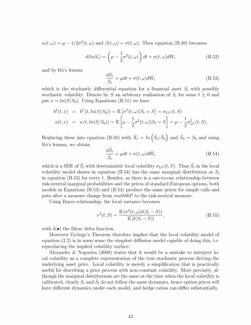
α(t, ω) = µ− 1/2σ2(t, ω) and β(t, ω) = σ(t, ω). Then εquation (B.49) becomes

d(lnSt) =

(µ− 1

2σ2(t, ω)

)dt+ σ(t, ω)dWt (B.52)

and by Ito’s lemmadStSt

= µdt+ σ(t, ω)dWt (B.53)

which is the stochastic differential equation for a financial asset St with possiblystochastic volatility. Denote by S an arbitrary realisation of St for some t ≥ 0 andput x = ln(S/S0). Using Equations (B.51) we have

b2(t, x) = b2 (t, ln(S/S0)) = E[σ2(t, ω)|St = S

]= σLV (t, S)

a(t, x) = a (t, ln(S/S0)) = E[µ− 1

2σ2(t, ω)|St = S

]= µ− 1

2σ2LV (t, S).

Replacing these into εquation (B.50) with Xt = ln(St/S0

)and S0 = S0 and using

Ito’s lemma, we obtaindSt

St= µdt+ σ(t, ω)dWt (B.54)

which is a SDE of St with deterministic local volatility σLV (t, S). Thus St in the localvolatility model shown in εquation (B.54) has the same marginal distribution as Stin εquation (B.53) for every t. Besides, as there is a one-to-one relationship betweenrisk-neutral marginal probabilities and the prices of standard European options, bothmodels in Equations (B.53) and (B.54) produce the same prices for simple calls andputs after a measure change from mathbbP to the risk-neutral measure.

Using Bayes relationship, the local variance becomes

v2(t, S) =E (σ2(t, ω)δ(St − S))

E [δ(St − S)], (B.55)

with δ(•) the Dirac delta function.Moreover Gyongy’s Theorem therefore implies that the local volatility model of

εquation (2.2) is in some sense the simplest diffusion model capable of doing this, i.e.reproducing the implied volatility surface.

Alexander & Nogueira (2008) states that it would be a mistake to interpret lo-cal volatility as a complete representation of the true stochastic process driving theunderlying asset price. Local volatility is merely a simplification that is practicallyuseful for describing a price process with non-constant volatility. More precisely, al-though the marginal distributions are the same at the time when the local volatility iscalibrated, clearly St and St do not follow the same dynamics, hence option prices willhave different dynamics under each model, and hedge ratios can differ substantially.

43

Bibliography

References

Alexander, C., & Nogueira, L. (2008). Stochastic Local Volatility . Technical Re-port DP2008-02 ICMA Centre. URL: http://carolalexander.org/publish/

download/DiscussionPapers/DP2008_02.pdf.

Andersen, L., & Andreasen, J. (2000). Jump diffusion processees: Volatility smilefitting and numerical methods for option pricing. Review of Derivatives Research,4 , 231–261.

Atlan, M. (2006). Localizing volatilities. arXiv:math/0604316 [math.PR]http://arxiv.org/abs/math/0604316v1 , .

Ayache, E., Henrotte, P., Nassar, S., & Wang, X. (2004). Can anyone solve the smileproblem? Wilmott Magazine, (pp. 78–96).

Bennett, C., & Gil, M. (2012). Volatility Trading: Trading Volatility, Correlation,Term Structure and Skew . Technical Report Santander Global Banking and Mar-kets. URL: http://cfe.cboe.com/education/TradingVolatility.pdf equityDerivatives.

Black, F. (1988). The holes in black-scholes. Risk , 1 , 30–32.

Bouzoubaa, M., & Osserein, A. (2010). Exotic Options and Hybrids: A Guide toStructuring, Pricing and Trading . Wiley Finance.

Breeden, D., & Litzenberger, R. (1978). Prices of state contingent claims implicit inoptions price. The Journal of Business , 51 , 621–651.

Brigo, D., & Mercurio, F. (2001). Interest Rate Models: Theory and Practice.Springer.

Brunick, G., & Shreve, S. (2013). Mimicking and ito process by a solution of astochastic differential equation. The Annals of Applied Probability , 23 , 1584–1628.

Carr, P., Fisher, T., & Ruf, J. (2013). Why are quadratic normal volatility modelsanalytically tractable? SIAM Journal on Financial Mathematics , 4(1), 185–202.

Castagna, A. (2010). FX Options and Smile Risk . Wiley Finance.

Clark, I. (2011). Foreign exchange option pricing . Wiley Finance.

Coleman, T., Li, Y., & Verma, A. (1999). Reconstructing the unknown local volatilityfunction. Journal of Computational Finance, 2 , 77–100.

Cozzi, D. (2012). Local Stochastic Volatility Models . Master’s thesis Politechnicodi Milano Italy. URL: https://www.politesi.polimi.it/bitstream/10589/

72489/1/2012_12_Cozzi.pdf.

44

Derman, E., & Kani, I. (1994). Riding on a smile. RISK Magazine, 1 , 32–39.

Derman, E., Kani, I., & Zou, J. (1995). The local volatility surface: Unlocking theinformation in index option prices. Goldman Sachs Quantitative Strategies ResearchNotes , December , 32–39.

Duffie, D. (1996). Dynamic Assep Pricing Theory . Princeton University Press.

Dumas, B., Fleming, J., & Whaley, R. (1998). Whaley, implied volatility functions:Empirical tests. Journal of Finance, 53 .

Dupire, B. (1993). Pricing and hedging with smiles. Paribas Capital Markets Swapsand Options Research Team, (pp. 1–9).

Dupire, B. (1994). Pricing with a smile. RISK Magazine, 1 , 18–20.

Engelmann, B., Fengler, M., & Schwendner, P. (2009). Better than its reputation: Anempirical hedging analysisof the local volatility model for barrier options. Journalof Risk , 12 , 53–77.

Gatheral, J. (2006). The Volatility Surface: A Practitioner’s Guide. New York, JohnWiley and Sons.

Gyongy, I. (1986). Mimicking the one-dimensional marginal distributions of processeshaving an ito differential. Probability Theory and Related Fields , 71 , 501–516.

Haugh, M. (2010). Beyond Black-Scholes . Technical Report Columbia University.URL: http://www.columbia.edu/~mh2078/LocalStochasticJumpDiffusion.

pdf iEOR E4707: Financial Engineering: Continuous Time Models.

Heston, S. (1993). A closed-form solution for options with stochastic volatility withapplications to bond and currency options. Review of Financial Studies , 10 , 327–343.

Hull, J. (2012). Options, Futures, and other Derivatives . Pearson.

Hull, J., & White, A. (1993). The pricing of options with stochastic volatilities.Journal of Finance, 42 , 281–300.

Kani, I., Derman, E., & Kamal, M. (1996). Trading and hedging local volatility.Goldman Sachs Quantitative Strategies Research Notes , August .

Klebaner, F. (2005). Introduction to Stochastic Calculus With Applications, SecondEdition. London, UK: Imperial College Press.

Kotze, A. (2003). Black-scholes or black holes? The South African Financial MarketsJournal , 2 , 8–12.

45

Kotze, A., & Joseph, A. (2009). Constructing a South African In-dex Volatility Surface from Exchange Traded Data. Technical Re-port Johannesburg Stock of Exchange, Equity Derivative, Report.Https://www.jse.co.za/content/JSEEducationItems/Generating South AfricanVolatility Surface.pdf.

Kotze, A., Labuschagne, C., Nair, M., & Padayachi, N. (2013). Arbitrage-free impliedvolatility surfaces for options on single stock futures. The North American Journalof Economics and Finance, 26 , 380–399.

Kotze, A., & Oosthuizen, R. (2013). Jse exotic can-do options: determining initialmargins. The South African Financial Markets Journal , 17 . URL: http://www.financialmarketsjournal.co.za/17thedition/jseequity.htm.

Kou, S. (2002). A jump diffusion model for pricing options. Management Science,48 , 1086–1101.

Lagnado, R., & Osher, S. (1997). Reconciling differences. RISK Magazine, 1 , 79–83.

Linetsky, V. (1998). The path integral approach to financial modeling and optionspricing. Computational Economics , 11 , 129–163.

Madan, D., & Seneta, E. (1990). The variance gamma model for share market returns.Journal of Business , 63 , 511–524.

Merton, R. (1976). Option pricing when the underlying stocks are discontinuous.Journal of Financial Economics , 5 , 125–14.

Pitarberg, Y. (2007). Markovian projection for volatility calibration. Risk Magazine,20 , 84–89.

Rebonato, R. (2004). Volatility and Correlation: the Perfect Hedger and the Fox,2ndEdition. John Wiley & Sons.

Rubinstein, M. (1994). Implied binomial trees. Journal of Finance, 49 , 771–818.

Wilmott, P. (1998). Derivatives . John Wiley and Sons.

46