IN IEEE TRANS. ON PATTERN ANALYSIS AND MACHINE INTELLIGENCE (PAMI), 2017 - TO APPEAR 1

Local Submodularizationfor Binary Pairwise Energies

Lena Gorelick, Yuri Boykov, Olga Veksler, Ismail Ben Ayed, Andrew Delong

Abstract—Many computer vision problems require optimization of binary non-submodular energies. We propose a generaloptimization framework based on local submodular approximations (LSA). Unlike standard LP relaxation methods that linearize thewhole energy globally, our approach iteratively approximates the energy locally. On the other hand, unlike standard local optimizationmethods (e.g., gradient descent or projection techniques) we use non-linear submodular approximations and optimize them withoutleaving the domain of integer solutions. We discuss two specific LSA algorithms based on trust region and auxiliary function principles,LSA-TR and LSA-AUX. The proposed methods obtain state-of-the-art results on a wide range of applications such as binarydeconvolution, curvature regularization, inpainting, segmentation with repulsion and two types of shape priors. Finally, we discuss amove-making extension to the LSA-TR approach. While our paper is focused on pairwise energies, our ideas extend to higher-orderproblems. The code is available online.

Index Terms—Discrete optimization, graph cuts, trust region, auxiliary functions, local submodularization.

F

1 INTRODUCTION

W E address a general class of binary pairwise non-submodular energies, which are widely used in applica-

tions like segmentation, stereo, inpainting, deconvolution, andmany others. Without loss of generality, the corresponding binaryenergies can be transformed into the form1

E(S) = STU + STMS, S ∈ 0, 1Ω (1)

where S = (sp ∈ 0, 1 | p ∈ Ω) is a vector of binary indicatorvariables defined on pixels p ∈ Ω, vector U = (up ∈ R | p ∈ Ω)represents unary potentials, and symmetric matrix M = (mpq ∈R | p, q ∈ Ω) represents pairwise potentials. Note that in manypractical applications matrix M is sparse since elements mpq = 0for all non-interacting pairs of pixels. We seek solutions to thefollowing integer quadratic optimization problem

minS∈0,1Ω

E(S). (2)

When energy (1) is submodular, i.e., mpq ≤ 0 ∀(p, q), globallyoptimal solution for (2) can be found in a low-order polynomialtime using graph cuts [1]. The general non-submodular case ofproblem (2) is NP hard.

1.1 Standard linearization methods

Integer quadratic programming is a well-known challenging classof optimization problems with extensive literature in the combi-natorial optimization community, e.g., see [1], [2], [3]. It often

• L. Gorelick, Y. Boykov, O. Veksler are with the Department of ComputerScience, University of Western Ontario, London, Canada. Andrew Delongis with the Department of Electrical Engineering, University of Toronto,Toronto, Canada.E-mail: lenagorelick@gmail.com

• Ismail Ben Ayed is with Departement de genie de la production automa-tisee, Ecole de Technologie Superieure, Montreal, Quebec, Canada

• Andrew Delong is with the Department of Electrical Engineering,University of Toronto, Toronto, Canada.

1. Note that such transformations are up to a constant, see Sec. 3.1.

LPE∇−

x * s0

sint

s*

oE∇− srlx

(a) global linearization (b) local linearization

Fig. 1. Standard linearization approaches for (1)-(2). Black dots areinteger points and ∗ corresponds to the global optimum of (2). Colorsin (b) show iso-levels of the quadratic energy (1). This energy can belinearized by introducing additional variables and linear constraints, seea schematic polytope in (a) and [6]. Vector ∇E is the gradient of theglobal linearization of (1) in (a) and the gradient of the local linearapproximation of (1) at point S0 in (b).

appears in computer vision where it can be addressed withmany methods including spectral and semi-definite programmingrelaxations, e.g., see [4], [5].

Methods for solving (2) based on LP relaxations, e.g., QPBO[7] and TRWS [8], are considered among the most powerful incomputer vision [9]. They approach integer quadratic problem(2) by global linearization of the objective function at a costof introducing a large number of additional variables and linearconstraints. These methods attempt to optimize the relaxed LP orits dual. However, the integer solution can differ from the relaxedsolution circled in Fig.1(a). This is a well-known integrality gapproblem. Most heuristics for extracting an integer solution fromthe relaxed solution have no a priori quality guarantees.

Our work is more closely related to local linearization tech-niques for approximating (2), e.g., parallel ICM, IPFP [10], andother similar methods [11]. Parallel ICM iteratively linearizesenergy E(S) around current solution S0 using Taylor expansionand makes a step by computing an integer minimizer Sint ofthe corresponding linear approximation, see Fig.1(b). However,

IN IEEE TRANS. ON PATTERN ANALYSIS AND MACHINE INTELLIGENCE (PAMI), 2017 - TO APPEAR 2

similarly to Newton’s methods, this approach often gets stuckin bad local minima by making too large steps regardless ofthe quality of the approximation. IPFP attempts to escape suchminima by reducing the step size. It explores the continuous linebetween integer minimizer Sint and current solution S0 and findsoptimal relaxed solution Srlx with respect to the original quadraticenergy. Similarly to the global linearization methods, see Fig.1(a),such continuous solutions give no quality guarantees with respectto the original integer problem (2).

1.2 Overview of submodularization

Linearization is a popular approximation approach to integerquadratic problem (1)-(2), but it often requires relaxation leadingto the integrality gap problem. We propose a different approxi-mation approach that we call submodularization. The main ideais to use submodular approximations of energy (1). We proposeseveral approximation schemes that keep submodular terms in (1)and linearize non-submodular potentials in different ways leadingto different optimization algorithms. Standard truncation of non-submodular pairwise terms2 and some existing techniques forhigh-order energies [12], [13], [14], [15] can be seen as submod-ularization examples, as discussed later. Common properties ofsubmodularization methods is that they compute globally optimalinteger solution of the approximation and do not leave the domainof discrete solutions avoiding integrality gaps. Sumbodularizationcan be seen as a generalization of local linearization methods sinceit uses more accurate higher-order approximations.

One way to linearize non-submodular terms in (1) is to com-pute their Taylor expansion around current solution S0. Taylor’sapproach is similar to IPFP [10], but they linearize all terms in-cluding submodular ones. In contrast to IPFP, our overall approx-imation of E(S) at S0 is not linear; it belongs to a more generalclass of submodular functions. Such non-linear approximationsare more accurate while still permitting efficient optimization inthe integer domain.

We also propose a different mechanism for controlling the stepsize. Instead of exploring relaxed solutions on continuous interval[S0, Sint] in Fig.1, (b), we obtain discrete candidate solutionS by minimizing local submodular approximation over 0, 1Ωunder additional distance constraint ||S − S0|| < d. Thus, ourapproach avoids integrality gap issues. For example, even linearapproximation model in Fig.1, (b) can produce solution S∗ ifHamming distance constraint ||S − S0|| ≤ 1 is imposed. Thislocal submodularization approach to (1)-(2) fits a general trustregion framework [4], [12], [16], [17]. We call it LSA-TR.

Another way to linearize the non-submodular terms in (1) isbased on the general auxiliary function framework [13], [15],[18]3. Instead of Taylor expansion, non-submodular terms inE(S) are approximated by linear upper bounds specific to currentsolution S0. Combining them with submodular terms in E(S)gives a submodular upper-bound approximation, a.k.a. an auxil-iary function, for E(S) that can be globally minimized within theinteger domain. This approach does not require to control the stepsize as the global minimizer of an auxiliary function is guaranteedto decrease the original energyE(S). We refer to this type of localsubmodular approximation approach as LSA-AUX.

2. Truncation is known to give low quality results, e.g. Fig.4, Tab.1.3. Auxiliary functions are also called surrogate functions or upper bounds.

The corresponding approximate optimization technique is also known as themajorize-minimize principle [18].

Recently both trust region [4], [16], [17] and auxiliary function[18] frameworks proved to work well for optimization of energieswith high-order regional terms [12], [15]. They derive specificlinear [12] or upper bound [15] approximations for non-linearcardinality potentials, KL and other distances between segmentand target appearance models. To the best of our knowledge, weare the first to develop trust region and auxiliary function methodsfor integer quadratic optimization problems (1)-(2).

In the context of multilabel energy minimization, there is aseries of works [19], [20], [21] that overestimate the intractableenergy with a tractable modified version within a move makingframework. Interestingly, instead of using linear (modular) upperbounds as in [13], [15], they change pairwise or higher-orderterms to achieve a submodular upper bound. Their approach isiterative due to the move-making strategy for multi-label energyoptimization, and would converge in a single step if reduced toour binary energy. In contrast, our approach is designed for binaryenergies and is iterative by definition.

In the context of binary high-order energies, more related toour to work are the auxiliary functions proposed in [13], [15]. In[15], Jensen inequality was used to derive linear upper bounds forseveral important classes of high-order terms that gave practicallyuseful results. Their approach is not directly applicable to ourenergy, as it is not clear which continuous function to use in theJensen inequality for our discrete pairwise energy.

The work in [13] is most related to ours. They divide theenergy into submodular and supermodular parts and replace thelatter with a certain permutation-based linear upper-bound. Thecorresponding auxiliary function allows polynomial-time solvers.However, experiments in [14] (Sec. 3.2) demonstrated limitedaccuracy of the permutation-based bounds [13] on high-ordersegmentation problems. Our LSA-AUX method is first to ap-ply auxiliary function approach to arbitrary (non-submodular)pairwise energies. We discuss possible linear upper bounds forpairwise terms and study several specific cases. One of themcorresponds to the permutation bounds [13] and is denoted byLSA-AUX-P. Recently [22] propose a generalization of [13] forhigher order binary energies. In the pairwise case, their approachis equivalent to LSA-AUX-P.

In [23] they relax the upper-bound condition and replace itwith a family of pseudo-bounds, which can better approximate theoriginal energy. According to their evaluation, LSA-TR performsbetter than their approach in most cases.

Our contributions can be summarized as follows:• A general submodularization framework for solving in-

teger quadratic optimization problems (1)-(2) based onlocal submodular approximations (LSA). Unlike globallinearization methods, LSA constructs an approximationmodel without additional variables. Unlike local lineariza-tion methods, LSA uses a more accurate approximation.

• In contrast to the majority of standard approximationmethods, LSA works strictly within the domain of discretesolutions and requires no rounding.

• We develop move making extension to the LSA approach,which can perform better on difficult energies.

• We propose a novel Generalized Compact shape prior thatrequires optimization of binary non-submodular energy.

• State-of-the-art results on a wide range of applications.Our LSA algorithms outperform QPBO, LBP, IPFP,TRWS, its latest variant SRMP, and other standard tech-niques for (1)-(2).

IN IEEE TRANS. ON PATTERN ANALYSIS AND MACHINE INTELLIGENCE (PAMI), 2017 - TO APPEAR 3

2 DESCRIPTION OF LSA ALGORITHMS

In this section we discuss our framework in detail. Section 2.1derives local submodular approximations and describes how toincorporate them in the trust region framework. Section 2.2 brieflyreviews auxiliary function framework and shows how to derivelocal auxiliary bounds.

2.1 LSA-TR

Trust region methods are a class of iterative optimization algo-rithms. In each iteration, an approximate model of the optimizationproblem is constructed near the current solution S0. The approx-imation is assumed to be accurate only within a small regionaround the current solution called “trust region”. The approximatemodel is then globally optimized within the trust region to obtaina candidate solution. This step is called trust region sub-problem.The size of the trust region is adjusted in each iteration basedon the quality of the current approximation. For a review of TRframework see [17].

Below we provide details of our trust region approach tothe binary pairwise energy optimization (see pseudo-code inAlgorithm 1). The goal is to minimize E(S) in (1). This energycan be decomposed into submodular and supermodular partsE(S) = Esub(S) + Esup(S) such that

Esub(S) = STU + STM−S

Esup(S) = STM+S

where matrix M− with negative elements m−pq ≤ 0 representsthe set of submodular pairwise potentials and matrix M+ withpositive elements m+

pq ≥ 0 represents supermodular potentials.Given the current solution St energy E(S) can be approximatedby submodular function

Et(S) = Esub(S) + STUt + const (3)

where Ut = 2M+St. The last two terms in (3) are the first-orderTaylor expansion of supermodular part Esup(S).

While the use of Taylor expansion may seem strange in thecontext of functions of integer variables, Fig. 2, (a,b) illustrates itsgeometric motivation. Consider individual pairwise supermodularpotentials f(x, y) in

Esup(S) =∑pq

m+pq · spsq =

∑pq

fpq(sp, sq).

Coincidentally, Taylor expansion of each relaxed supermodularpotential f(x, y) = α·xy produces a linear approximation (planesin b) that agrees with f at three out of four possible discreteconfigurations (points A,B,C,D).

The standard trust region sub-problem is to minimize approx-imation Et within the region defined by step size dt

S∗ = argmin||S−St||<dt

Et(S). (4)

Hamming, L2, and other useful metrics ||S − St|| can be repre-sented by a sum of unary potentials [24]. However, optimizationproblem (4) is NP-hard even for unary metrics4. One can solveLagrangian dual of (4) by iterative sequence of graph cuts asin [25], but the corresponding duality gap may be large and theoptimum for (4) is not guaranteed.

4. By a reduction to the balanced cut problem.

Instead of (4) we use a simpler formulation of the trustregion subproblem proposed in [12]. It is based on unconstrainedoptimization of submodular Lagrangian

Lt(S) = Et(S) + λt · ||S − St|| (5)

where parameter λt controls the trust region size indirectly. Eachiteration of LSA-TR solves (5) for some fixed λt and adaptivelychanges λt for the next iteration (Alg.1 line 27), as motivatedby empirical inverse proportionality relation between λt and dtdiscussed in [12].

Once a candidate solution S∗ is obtained, the quality of theapproximation is measured using the ratio between the actual andpredicted reduction in energy. Based on this ratio, the solution isupdated in line 24 and the step size (or λ) is adjusted in line27. It is common to set the parameter τ1 in line 24 to zero,meaning that any candidate solution that decreases the actualenergy gets accepted. The parameter τ2 in line 27 is usually setto 0.25 [17]. Reduction ratio above this value corresponds to goodapproximation model allowing increase in the trust region size.

Algorithm 1: GENERAL TRUST REGION APPROACH

1 Initialize t = 0, St = Sinit, λt = λinit, convergedFlag = 02 While !convergedFlag3 //Approximate E(S) around St

4 Et(S) = Esub(S) + STUt as defined in (3)5 //Solve Trust Region Sub-Problem6 S∗ ←− argminS∈0,1Ω Lt(S) // as defined in (5)7 //Evaluate Reduction in Energy8 P = Et(St)− Et(S

∗) //predicted reduction in energy9 R = E(St)− E(S∗) //actual reduction in energy

10 If P = 0 // meaning S∗ = St and λ > λmax11 //Try smallest discrete step possible12 λt ←− λmax13 //Solve Trust Region Sub-Problem14 S∗ ←− argminS∈0,1Ω Lt(S) // as defined in (5)15 //Evaluate Reduction in Energy16 P = Et(St)− Et(S

∗) //predicted reduction in energy17 R = E(St)− E(S∗) //actual reduction in energy18 //Update current solution

19 St+1 ←−S∗ if R/P > τ1St otherwise

20 //Check Convergence21 convergedFlag←− (R ≤ 0)22 Else23 //Update current solution

24 St+1 ←−S∗ if R/P > τ1St otherwise

25 End26 //Adjust the trust region

27 λt+1 ←−λt/α if R/P > τ2λt · α otherwise

28 End

In each iteration of the trust region, either the energy decreasesor the trust region size is reduced. When the trust region is sosmall that it does not contain a single discrete solution, namelyS∗ = St (Line 10), one more attempt is made using λmax, whereλmax = sup λ|S∗ 6= St (see [12]). If there is no reduction inenergy with smallest discrete step λmax (Line 21), we are at a localminimum [26] and we stop.

2.2 LSA-AUXBound optimization techniques are a class of iterative optimiza-tion algorithms constructing and optimizing upper bounds, a.k.a.

IN IEEE TRANS. ON PATTERN ANALYSIS AND MACHINE INTELLIGENCE (PAMI), 2017 - TO APPEAR 4

(a) Supermodular potential α ·xy (b) “Taylor” based local linearization (c) Upper bound linearization

Fig. 2. Local linearization of supermodular pairwise potential f(x, y) = α · xy for α > 0. This potential defines four costs f(0, 0) = f(0, 1) =f(1, 0) = 0 and f(1, 1) = α at four distinct configurations of binary variables x, y ∈ 0, 1. These costs can be plotted as four 3D points A, B, C, Din (a-c). We need to approximate supermodular potential f with a linear function v · x+w · y+ const (plane or unary potentials). LSA-TR: one wayto derive a local linear approximation is to take Taylor expansion of f(x, y) = α · xy over relaxed variables x, y ∈ [0, 1], see the continuous plot in(a). At first, this idea may sound strange since there are infinitely many other continuous functions that agree with A, B, C, D but have completelydifferent derivatives, e.g., g(x, y) = α · x2√y. However, Taylor expansions of bilinear function f(x, y) = α · xy can be motivated geometrically. Asshown in (b), Taylor-based local linear approximation of f at any fixed integer configuration (i, j) (e.g., . blue plane at A, green at B, orange at C,and striped at D) coincides with discrete pairwise potential f not only at point (i, j) but also with two other closest integer configurations. Overall,each of those planes passes exactly through three out of four points A, B, C, D. LSA-AUX: another approach to justify a local linear approximationfor non-submodular pairwise potential f could be based on upper bounds passing through a current configuration. For example, the green or orangeplanes in (b) are the tightest linear upper bounds at configurations (0, 1) and (1, 0), correspondingly. When current configuration is either (0, 0) or(1, 1) then one can choose either orange or green plane in (b), or anything in-between, e.g., the purple plane passing though A and D in (c).

auxiliary functions, for energy E. It is assumed that those boundsare easier to optimize than the original energy E. Given a currentsolution St, the function At(S) is an auxiliary function of E if itsatisfies the following conditions:

E(S) ≤ At(S) (6a)

E(St) = At(St) (6b)

To approximate minimization of E, one can iteratively minimizea sequence of auxiliary functions:

St+1 = arg minS

At(S) , t = 1, 2, . . . (7)

Using (6a), (6b), and (7), it is straightforward to prove that thesolutions in (7) correspond to a sequence of decreasing energyvalues E(St). Namely,

E(St+1) ≤ At(St+1) ≤ At(St) = E(St).

The main challenge in bound optimization approach is design-ing an appropriate auxiliary function satisfying conditions (6a) and(6b). However, in case of integer quadratic optimization problem(1)-(2), it is fairly straightforward to design an upper bound fornon-submodular energy E(S) = Esub(S) + Esup(S). As inSec.2.1, we do not need to approximate the submodular part Esub

and we can easily find a linear upper bound for Esup as follows.Similarly to Sec.2.1, consider supermodular pairwise poten-

tials f(x, y) = α · xy for individual pairs of neighboring pixelsaccording to

Esup(S) =∑pq

m+pq · spsq =

∑pq

fpq(sp, sq) (8)

where each fpq is defined by scalar α = m+pq > 0. As shown

in Fig. 2, (b,c), each pairwise potential f can be bound above bylinear function u(x, y)

f(x, y) ≤ u(x, y) := v · x+ w · y

for some positive scalars v and w. Assuming current solution(x, y) = (xt, yt), the table below specifies linear upper bounds(planes) for four possible discrete configurations

(xt, yt) upper bound u(x, y) plane in Fig.2(b,c)(0,0) α

2 x+ α2 y purple

(0,1) αx green(1,0) αy orange(1,1) α

2 x+ α2 y purple

We denote the approach that uses bounds in the table aboveas LSA-AUX. As clear from Fig.2, (b,c), there are many otherpossible linear upper bounds for pairwise terms f . Interestingly,the “permutation” approach to high-order supermodular terms in[13] reduces to linear upper bounds for f(x, y) where each config-uration (0,0) or (1,1) selects either orange or green plane randomly(depending on a permutation). We denote permutation based upperbounds LSA-AUX-P. Our tests showed inferior performance ofsuch bounds for pairwise energies compared to LSA-AUX on mostapplications. The upper bounds using purple plane for (0,0) and(1,1), as in the table, work better in practice.

Summing upper bounds for all pairwise potentials fpq in (8)using linear terms in this table gives an overall linear upper boundfor supermodular part of energy (1)

Esup(S) ≤ STUt (9)

where vector Ut = utp|p ∈ Ω consists of elements

utp =∑q

m+pq

2(1 + stq − stp)

and St = stp|p ∈ Ω is the current solution configuration for allpixels. Defining our auxiliary function as

At(S) := STUt + Esub(S) (10)

and using inequality (9) we satisfy condition (6a)

E(S) = Esup(S) + Esub(S) ≤ At(S).

Since STt Ut = Esup(St) then our auxiliary function (10) alsosatisfies condition (6b)

E(St) = Esup(St) + Esub(St) = At(St).

IN IEEE TRANS. ON PATTERN ANALYSIS AND MACHINE INTELLIGENCE (PAMI), 2017 - TO APPEAR 5

0.05 0.1 0.15 0.20

50

100

150

200

250

300

350

Noise σ

Ene

rgy

LBPQPBO-IIPFPLSA-AUX-PLSA-AUXLSA-TR(-L)TRWSSRMP

Img + N(0,0.05)

LSA-TR(0.3 sec.)

LSA-AUX (0.04 sec)

TRWS

LBP QPBO(0.1 sec.)

QPBO-I(0.2 sec.)

IPFP(0.4 sec.)

LSA-AUX-P (0.13 sec)

SRMP

Fig. 3. Binary deconvolution of an image created with a uniform 3 × 3filter and additive Gaussian noise (σ ∈ 0.05, 0.1, 0.15, 0.2). No lengthregularization was used. We report mean energy (+/-2std.) and time asa function of noise level σ. TRWS, SRMP and LBP are run for 5000iterations.

Function At(S) is submodular. Thus, we can globally optimize itin each iteration guaranteeing an energy decrease.

3 APPLICATIONS

Below we apply our method in several applications such as binarydeconvolution, segmentation with repulsion, curvature regulariza-tion, inpainting and two different shape priors, one of which is anovel contribution by itself. We report results for both LSA-TRand LSA-AUX frameworks and compare to existing state of theart methods such as QPBO [7], LBP [27], IPFP [10], TRWS andSRMP [8] in terms of energy and running time5. For the sakeof completeness, and to demonstrate the advantage of non-linearsubmodular approximations over linear approximations, we alsocompare to a version of LSA-TR where both submodular andsupermodular terms are linearized, denoted by LSA-TR-L.

In the following experiments, all local approximation methods,e.g., IPFP, LSA-AUX, LSA-AUX-P, LSA-TR, LSA-TR-L areinitialized with the entire domain assigned to the foreground. Allglobal linearization methods, e.g., TRWS, SRMP and LBP, arerun for 50, 100, 1000 and 5000 iterations. For QPBO results,unlabeled pixels are shown in gray color. Running time is shown inlog-scale for clarity. Our preliminary experiments showed inferiorperformance of the Hamming distance compared to Euclidean.See example in Sec. 3.5. Therefore, we used L2 distance for allthe experiments below.

5. We used http://pub.ist.ac.at/∼vnk/software.html code for SRMP andwww.robots.ox.ac.uk/∼ojw code for QPBO, TRWS, and LBP. The correspond-ing version of LPB is sequential without damping.

TRWS LSA-TRLSA-AUX

QPBO QPBO-I LBP w/o repuls.

LSA-TR-L

IPFP

PairwisePotentials

Unary Potentials

Img

100 102-300

-200

-100

0

100

200

Time

Ene

rgy

LBPQPBO-IIPFPLSA-AUX-PLSA-AUXLSA-TRTRWSLower Bound TRWSSRMPLower Bound SRMP

LSA-AUX-PSRMP

Fig. 4. Segmentation with repulsion and attraction. We used µfg=0.4,µbg=0.6, σ=0.2 for appearance, λreg=100 and c=0.06. Repulsion po-tentials are shown in blue and attraction - in red.

3.1 Energy Transformation

For some applications, instead of defining the energy as in (1), itis more convenient to use the following form:

E(S) =∑p∈Ω

Dp(sp) +∑

(p,q)∈N

Vpq(sp, sq), (11)

where Dp is the unary term, Vpq is the pairwise term and N is aset of ordered neighboring pairs of variables. We now explain howto transform the energy in (11) to the equivalent form in (1).

Transformation of the unary terms Dp results in a linear term(i.e., vector) J = (jp|p ∈ Ω), where jp = Dp(1)−Dp(0).

Let the pairwise terms Vpq(sp, sq) be as follows:

sp sq Vpq0 0 apq0 1 bpq1 0 cpq1 1 dpq

Transformation of the pairwise terms Vpq results in two linearterms H,K one quadratic term M and a constant. Term Haccumulates for each variable p all Vpq in which p is the firstargument. That is,

H = (hp|p ∈ Ω),where hp =∑

(p,q)∈N

(cpq − apq).

Term K does the same for the second argument of Vpq . That is,

K = (kq|q ∈ Ω),where kq =∑

(p,q)∈N

(bpq − apq).

We define quadratic termM in (1) asmpq = apq−bpq−cpq+dpq .Letting U = J + H + K and M as defined above, it is easy

to show that the energy in (11) can be written in the form of (1)up to a constant C =

∑pDp(0) +

∑(p,q)∈N apq .

IN IEEE TRANS. ON PATTERN ANALYSIS AND MACHINE INTELLIGENCE (PAMI), 2017 - TO APPEAR 6

LSA-AUX-P LSA-AUX LSA-TR TRWS SRMPLBP IPFP QPBO

λ=0.1

Image

QPBO-I

λ=0.5

Image LSA-AUX-P LSA-AUX LSA-TR SRMP IPFP QPBOLBP

QPBO-ILSA-AUX-P LSA-AUX LSA-TR SRMP IPFP QPBO

λ=2

Image LBP

TRWS

TRWS

10-5 100-5000

-4000

-3000

-2000

-1000

0

1000

2000

Time

Ene

rgy

10-0.45 10-0.3565

70

75

80

Time

Ener

gy

λ=0.5

10-2 100 1020

500

1000

1500

2000

2500

TimeEn

ergy

10-2 100 102-2.25

-2.24

Time

≈

LBPQPBO-IIPFPLSA-AUX-PLSA-AUXLSA-TRTRWSLower Bound TRWSSRMPLower Bound SRMP

λ=2

Fig. 5. Curvature regularizer [28] is more difficult to optimize when regularizer weight is high. We show segmentation results for λcurv = 0.1 (toprow), λcurv = 0.5 (middle row), λcurv = 2 (bottom row) as well as energy plots. We used µfg = 1, µbg = 0, λapp = 1.

3.2 Binary Deconvolution

Figure 3, (top-left) shows a binary image after convolution with auniform 3×3 combined with Gaussian noise (σ = 0.05). The goalof binary deconvolution is to recover the original binary image.The energy is defined as

E(S) =∑p∈Ω

(Ip −1

9

∑q∈Np

sq)2 (12)

HereNp denotes the 3×3 neighborhood window around pixelp and all pairwise interactions are supermodular. We did not uselength regularization, since it would make the energy easier tooptimize. Figure 3 compares the performance of LSA-TR andLSA-AUX to standard optimization methods such as QPBO, LBP,IPFP, TRWS and SRMP. In this case LSA-TR-L and LSA-TRare identical since energy (12) has no submodular pairwise terms.The bottom of Fig. 3 shows the mean energy as a function ofnoise level σ. For each experiment the results are averaged overten instances of random noise. The mean time is reported for theexperiments with σ = 0.05.

3.3 Segmentation with Repulsion

In this section we consider segmentation with attraction andrepulsion pairwise potentials. Adding repulsion is similar to cor-relation clustering [29] and multiway cut [30], where data pointseither attract or repulse each other. Using negative repulsion insegmentation can avoid the bias of submodular length regularizerto short-cutting, whereby elongated structures are shortened toavoid high length penalty. Figure 4 (top-left) shows an example

of an angiogram image with elongated structures. We use 16-neighborhood system and the pairwise potentials are defined asfollows:

ω(p, q) =−∆(p, q) + c

dist(p,q).

Here dist(p,q) denotes the distance between image pixels p andq and ∆(p, q) is the difference in their respective intensities(see pairwise potentials in Fig. 4, bottom-left). The constant cis used to make neighboring pixels with similar intensities attractand repulse otherwise. Being supermodular, repulsions potentialsmake the segmentation energy more difficult to optimize, but arecapable to extract thin elongated structures. To demonstrate theusefulness of “repulsion” potentials we also show segmentationresults with graph-cut a la Boykov-Jolly [31] where negativepairwise potentials were removed/truncated (top-right).

3.4 Curvature

Below we apply our optimization method to curvature regular-ization. We focus on the curvature model proposed in [28]. Themodel is defined in terms of 4-neighborhood system and accountsfor 90 degrees angles. In combination with appearance terms, themodel yields discrete binary energy that has both submodular andnon-submodular pairwise potentials. Originally, the authors of [28]proposed using QPBO for optimization of the curvature regular-izer. We show that our method significantly outperforms QPBOand other state-of-the-art optimization techniques, especially withlarge regularizer weights.

First, we deliberately choose a toy example (white circle on ablack background, see Fig. 5), where we know what an optimal

IN IEEE TRANS. ON PATTERN ANALYSIS AND MACHINE INTELLIGENCE (PAMI), 2017 - TO APPEAR 7

solution should look like. With the 4-neighborhood system, asthe weight of the curvature regularizer increases, the solutionshould minimize the number of 90 degrees angles (corners) whilemaximizing the appearance terms. Therefore, when the weight ofcurvature regularizer is high, the solution should look more like asquare than a circle. Consider the segmentation results in Fig. 5.With low curvature weight, λcurv = 0.1 , all compared methodsperform equally well (see top row). In this case appearancedata terms are strong compared to the non-submodular pairwiseterms. However, when we increase the curvature weight and setλcurv = 0.5 or 2 there is a significant difference between theoptimization methods both in terms of the energy and the resultingsolutions (see Fig. 5 middle and bottom).

Next, we selected an angiogram image example from [28] andevaluate the performance6 of the optimization methods with twovalues of regularizer weight λcurv = 19 and λcurv = 21 (seeFig. 6). Although the weight λ did not change significantly, thequality of the segmentation deteriorated for all global linearizationmethods, namely QPBO, TRWS, LBP. The proposed methodsLSA-TR and LSA-AUX seem to be robust with respect to theweight of the supermodular part of the energy.

3.5 Chinese Characters Inpainting

Below we consider the task of in-painting in binary images ofChinese characters, dtf-chinesechar [9]. We used a set of pre-trained unary and pairwise potentials provided by the authors withthe dataset. While each pixel variable has only two possible labels,the topology of the resulting graph and the non-submodularity ofits pairwise potentials makes this problem challenging. Figure 7shows two examples of inpainting. Table 1 reports the performanceof our LSA-TR and LSA-AUX methods on this problem andcompares to other standard optimization methods reported in [9],as well as, to truncation of non-submodular terms. LSA-TR isranked second, but runs four orders of magnitudes faster.

3.6 Segmentation of Multi-Region Objects

Many objects can be described by a combination of spatiallycoherent and visually distinct regions. Such objects can oftenbe segmented using multi-label segmentation framework, where aseparate appearance-boundary model is maintained for each label.Recently a multi-label segmentation model has been proposedin [32] that uses a separate binary graph layer for each labeland allows encoding many useful geometric interactions betweendifferent parts of an object. For example inclusion of an objectpart within another part while enforcing a minimal margin aroundthe interior part is modeled using submodular pairwise interac-tions between corresponding nodes in different layers. Exclusionconstraints are in general supermodular.

In this section we focus on one particular example of multi-partmodel designed for segmentation of liver on an MRI image, seeFig. 9, (a-left). The image contains one foreground object (liver)with four distinct mutually exclusive interior parts (tumors). Belowwe formally define the energy for our model using the form in (11).To convert this energy to the form in (1) see details in Sec. 3.1.

Given an image with N pixels, we construct a graph withfive layers of binary variables. The layers correspond to liver

6. For QPBO, we only run QPBO-I and do not use other post-processingheuristics as suggested in [28], since the number of unlabeled pixel might besignificant when the regularization is strong.

Alg.Name

MeanRuntime

MeanEnergy

#best/100 Rank

MCBC 2053.89sec

-49550.1 85 1

BPS (LBP)∗ 72.85 sec -49537.08 18 3ILP 3580.93

sec-49536.59 8 6

QPBO 0.16 sec -49501.95 0 8SA NaN sec -49533.08 13 4TRWS 0.13 sec -49496.84 2 7TRWS-LF 2106.94

sec-49519.44 11 5

Truncation 0.06 sec -16089.2 0 9LSA-AUX 0.30 sec -49515.95 0 9LSA-AUX-P 0.16 sec -49516.63 0 9LSA-TR(Euc.)

0.21 sec -49547.61 35 2

LSA-TR(Ham.)

0.23 sec -49536.76 1 8

TABLE 1Chinese characters in-painting database [9]. We tested three methods(at the bottom) and compared with other techniques (above) reported

in [9]. * - To the best of our knowledge, BPS in [9] is the basicsequential version of loopy belief-propagation without damping that we

simply call LBP in this paper.

(Fg), and four tumors (A, B, C, D). Each layer has N nodes andeach node has a corresponding binary variable. We use a standardPotts regularization on each layer to account for boundary lengthbetween object parts. In addition we employ pairwise inclusionand exclusion constraints between the layers to enforce correctgeometric interactions between the different parts of the object, seeFig. 8, (b). Finally we derive unary terms for the binary variablesso that they correspond to the correct multilabel appearance energyterm.

Each graph node p has three coordinates (rp, cp, lp) and acorresponding binary variable sp. The first two coordinates denotethe row and column of the corresponding pixel in the image (top-left corner as origin) and the last coordinate lp denotes the layerof the node, lp ∈ Fg,A,B,C,D.

For length regularization, we use 8-neighborhood systemwithin each layer and the pairwise potentials are defined asfollows. Let p, q be neighboring nodes in some layer l ∈A,B,C,D, then

V 1p,q(sp, sq) = λPotts

−∆(p, q)

dist(p,q)· [sp 6= sq].

Here dist(p,q) =√

(rp − rq)2 + (cp − cq)2 denotes the distancebetween the corresponding image pixels in the image domain,∆(p, q) is the distance between in their respective colors in theRGB color space and λPotts is the weight.

Next, we explain how to implement inclusion and exclusionconstraints, see Fig. 8, (b). Let p and q be two nodes correspondingto the same pixel such that node p is in the liver (Fg) layer andnode q is in a tumor layer. That is (rq = rp)∧(cq = cp) and (lp =Fg)∧(lq ∈ A,B,C,D). Inclusion pairwise potential V 2

p,q forcesany interior tumor part to be geometrically inside the foregroundobject by penalizing configuration (0, 1) for the correspondingnodes p, q. That is

V 2p,q(sp, sq) = λsub ·

∞ if (sp, sq) = (0, 1)

0 otherwise.

IN IEEE TRANS. ON PATTERN ANALYSIS AND MACHINE INTELLIGENCE (PAMI), 2017 - TO APPEAR 8

10-2 100 102 1040

2

4

6

8

10

12x 104

Time

Ene

rgy

10-2 100 102 104-0.5

0

0.5

1

1.5

2

2.5x 105

Time

Ene

rgy

LBP TRWS

QPBO QPBO-I

LSA-TR LSA-AUXIPFP

LBP TRWS

QPBO QPBO-I

LSA-TR

λ=21

IPFP LSA-AUX

SRMP

LSA-AUX-P

λ=21

LBPQPBO-IIPFPLSA-AUX-PLSA-AUXLSA-TRTRWSLower Bound TRWSSRMPLower Bound SRMP

λ=19

SRMP

LSA-AUX-P

λ=19 λ=21

Fig. 6. Curvature regularizer [28]: we show segmentation results and energy plots for λcurv=19 (left), λcurv=21 (right).

LSA-TRInput Img Ground Truth

Fig. 7. Examples of Chinese characters inpainting.

The tumor parts are mutually exclusive, see Fig. 8, (b). Let pand q be two nodes corresponding to the same image pixel but indifferent tumor layers. That is (rq = rp)∧ (cq = cp) and lp 6= lqwhere lp, lq ∈ A,B,C,D. Then the supermodular exclusionpairwise potential V 3

p,q penalizes illegal configuration (1, 1). Eachpixel can only belong to one tumor. That is,

V 3p,q(sp, sq) = λsup ·

∞ if (sp, sq) = (1, 1)

0 otherwise.

Since for each image pixel (r, c) we have five binary vari-ables (one in each layer), there are 25 possible configurations oflabels for each quintuple. However, our inclusion and exclusionconstraints render most of the configurations illegal, i.e., havinginfinite cost. Figure 8, (c) summarizes all legal configurationsfor each quintuple of variables, their interpretation in terms ofimage segmentation and the respective multilabel appearancecost Dr,c(l). Below, we define the unary terms Dp in (11) forour binary graph so that the binary energy corresponds to themultilabel energy in terms of appearance cost. Let p = (r, c, l) bea node in our graph and let Dr,c(l) be the multilabel appearanceterm at image pixel (r, c) for label l. Then,

Dp(sp) =

Drp,cp(Fg) if lp = Fg ∧ sp = 1

Drp,cp(Bg) if lp = Fg ∧ sp = 0

Drp,cp(lp)−Drp,cp(Fg) if lp ∈ A,B,C,D∧sp = 1

0 otherwise.

excludes

Bg

AB C

D

Fg

A B

D

C

Bg

Fg

Five Binary Labelsper Pixel in Our Graph

ImgPixelLabel

MultilabelCostD(r,c) (.)

Fg A B C D

0 0 0 0 0 Bg Dr,c(Bg)

1 0 0 0 0 Fg Dr,c(Fg)

1 1 0 0 0 A Dr,c (A)

1 0 1 0 0 B Dr,c (B)

1 0 0 1 0 C Dr,c (C)

1 0 0 0 1 D Dr,c (D)

Any other configuration

∞

(a)

(b) (c)

Fig. 8. Multi-part object model for liver segmentation: (a) schematicrepresentation of the liver containing four distinct and mutually excludingtumors. (b) each part of the object is represented with a separate binarylayer in the graph. Each image pixel has a corresponding node in all fivelayers, resulting in a quintuple (FG, A, B, C, D). Interactions betweencorresponding nodes of different layers are shown with black solid linesfor inclusion and blue dashed lines for exclusion. (c) summarizes sixlegal configurations for each pixel’s quintuple and the associated multi-label cost. All other configurations have an infinite cost due to inclusionor exclusion violations.

If each pixel’s quintuples is labeled with legal configuration, theunary appearance term on our graph is equal to the multilabelappearance term for image pixels.

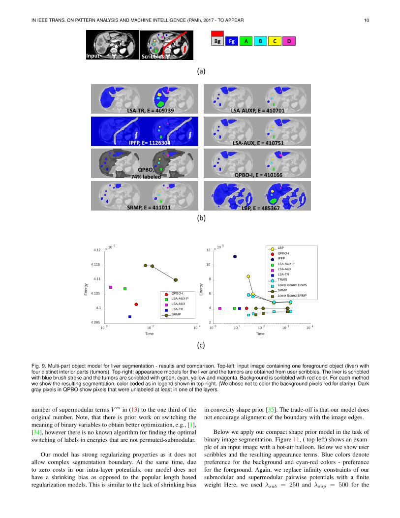
Below we apply our multi-part object prior model in the task ofmulti-label segmentation of liver with tumors on an MRI image.Figure 9, (a) shows an input image containing one foregroundobject (liver) with four distinct interior parts (tumors). Userscribbles are used to obtain appearance models for the liver and thetumors and as hard constraints. The liver is scribbled with the bluebrush stroke and the tumors are scribbled with the green, cyan,yellow and magenta. Background is scribbled with the red color.While in theory our model has infinity constraints, in practice weneed to select a finite weight for our submodular and supermodular

IN IEEE TRANS. ON PATTERN ANALYSIS AND MACHINE INTELLIGENCE (PAMI), 2017 - TO APPEAR 9

pairwise potentials. Here, we used λsub = λsup = 100 for theinclusion and exclusion terms respectively and λPotts = 25. Forappearance we used histograms with 16 bins per color channel.

Figure 9, (b) shows segmentation results and compares differ-ent methods. For each compared method we show the final imagesegmentation, color coded as in the legend. We chose not to colorthe background pixels red for clarity, but rather leave them lightgray. Dark gray pixels in QPBO denote pixels that were unlabeledat least in one of the five layers.

Figure 9, (c-right) compares the methods in terms of energyand the running time (shown in log-scale). The graph in (c-left)zooms in on the most interesting part of the plot. All the comparedmethods arrived at poor or very poor solutions that have violationsof inclusion and exclusion constraints. This is due to the largenumber of the supermodular terms. LSA-TR achieves the lowestenergy and the best segmentation.

3.7 Generalized Compact Shape Prior

In this section we propose a novel shape prior that is formulatedas a multilabel energy and is subsequently reduced to a binarynon-submodular pairwise energy using reduction similar to thatin Sec. 3.6. Our new model generalizes compact shape priorproposed in [33]. Compact shape prior is useful in industrial partdetection and medical image segmentation applications.

The compact shape prior in [33] assumes that an object canbe partitioned into four quadrants around a given object center,provided by the user. Within each quadrant an object contour iseither a monotonically decreasing or increasing function in theallowed direction for each quadrant. Figure 10, (a-top), shows anexample of an object (along with user provided center) that can besegmented using the model in [33]. Allowed orientations for eachquadrant are shown with blue arrows.We propose a more generalmodel. It does not require user interaction, nor it assumes an objectcenter, allowing for a larger class of object shapes.

Instead of dividing the whole object into four quadrants, ournew model explicitly divides the background into four regionsas in Fig. 10, (a-bottom), corresponding to four labels: top-left (TL), top-right (TR), bottom-left (BL), bottom-right (BR).There is an additional label for the foreground object (Fg). Eachbackground label allows discontinuities only in certain orientationas is illustrated with the blue arrows. For example, the red regioncan have discontinuity only in the up-right orientation. Our modelincludes the model proposed in [33] as a special case when thetransitions between different background labels are horizontallyand vertically aligned as in (a-bottom). However, our model ismore general because the discontinuities between the backgroundregions do not need to align. For example, the object in (b-top) canbe segmented using our model (b-bottom), but not the model in[33]. Below we formally define the energy for our model using theform in (11). To convert this energy to the form in (1) see detailsin Sec. 3.1.

Given an image with N pixels, we construct a graph withfour binary layers: TL, TR, BL, BR. Each layer has N nodesand each node has a corresponding binary variable. Each layer isresponsible for the respective region of the background and allowsdiscontinuities only in a certain direction. In addition, there arealso exclusion constraints between the layers to enforce a coherentforeground object, see Fig. 10, (c).

Each graph node p has three coordinates (rp, cp, lp) and acorresponding binary variable sp. The first two coordinates denote

the row and column of the corresponding pixel in the image (top-left corner as origin) and the last coordinate denotes the layer ofthe node, l ∈ TL,TR,BL,BR.

There are two types of pairwise potentials in our model. Thefirst type of potentials is defined between nodes within the samelayer. It maintains the allowed orientation of the correspondingregion boundary. For example, top-left layer TL allows switchingfrom label 0 to 1 in the right and upward directions. Formally,

V TLpq(sp, sq) =

=

∞ if (sp, sq) = (1, 0) ∧ (rq = rp) ∧ (cq = cp + 1)

∞ if (sp, sq) = (1, 0) ∧ (rq = rp + 1) ∧ (cq = cp)

0 otherwise.

Similar intra-layer pairwise potentials are defined on the otherthree layers.

The other type of pairwise potentials is defined betweencorresponding nodes of different layers. They are responsible forexclusion constraint between the different background labels, seeFig. 10, (c). For example the red region (TL) in Fig. 10, (a-bottom)cannot overlap any of the other background regions (TR, BL, BR).Such pairwise potentials are super-modular.

Let p and q be two nodes corresponding to the same imagepixel but in different graph layers. That is (rq = rp) ∧ (cq =cp) and lp 6= lq where lp, lq ∈ TR,TL,BR,BL. Then thesupermodular exclusion pairwise potential V ex

p,q penalizes illegalconfiguration (0, 0). That is

V expq(sp, sq) =

∞ if (sp, sq) = (0, 0)

0 otherwise.(13)

To interpret the optimal solution on our graph in terms ofbinary image segmentation, for each pixel we consider a quadrupleof corresponding binary variables on layers TR, TL, BR andBL. We assign image pixel to foreground object (fg) if all itscorresponding graph nodes have label one, and to the background(bg) otherwise, see table in Fig. 10, (d). As in [33], our modelcan incorporate any unary term in (11) defined on image pixels,e.g., appearance terms. We now define the corresponding unaryterms on the nodes of our four layers binary graph.

Let Dr,c(fg) and Dr,c(bg) be the costs of assigning imagepixel (r, c) to the foreground (fg) and background (bg) respec-tively. For each image pixel (r, c) we have a set of four corre-sponding graph nodes p = (rp, cp, lp)|(rp = r) ∧ (cp = c).All these nodes have the same unary term:

Dp(sp) =

Drp,cp(fg) if sp = 1

Drp,cp(bg) if sp = 0.

With the infinity constraints in our model, each image pixel (r, c)can have only two possible label configurations for the correspond-ing four graph nodes. It will either have three foreground and onebackground labels, in which case the image pixel is assigned tothe background with a cost of 3 ·Dr,c(fg)+Dr,c(bg). Or, all fournodes will have foreground labels, in which case the image pixelis assigned to the foreground with the cost of 4 ·Dr,c(fg). In bothcases, each image pixel will pay the additional constant cost of3 ·Dr,c(fg). This constant does not affect optimization.

Finally, we switch the meaning of zeros and ones for layersTR and BL. Labels 0 and 1 mean background and foregroundin layers TR and BL and switch their meaning in layers TLand BR. While the switch is not necessary, it reduces the total

IN IEEE TRANS. ON PATTERN ANALYSIS AND MACHINE INTELLIGENCE (PAMI), 2017 - TO APPEAR 10

10 0 10 1 10 2 10 3 10 4

Time

2

4

6

8

10

12

Ene

rgy

10 5LBP

QPBO-IIPFP

LSA-AUX-P

LSA-AUX

LSA-TRTRWS

Lower Bound TRWS

SRMPLower Bound SRMP

10 0 10 2 10 4

Time

4.095

4.1

4.105

4.11

4.115

4.12

Ene

rgy

10 5

QPBO-ILSA-AUX-PLSA-AUXLSA-TRSRMP

LSA-TR, E = 409739 LSA-AUXP, E = 410701

LSA-AUX, E = 410751IPFP, E= 1126304

LBP, E = 485367

QPBO, 74% labeled

SRMP, E = 411011

QPBO-I, E = 410166

Bg Fg A B C D

Input Scribbles

(a)

(b)

(c)

Fig. 9. Multi-part object model for liver segmentation - results and comparison. Top-left: input image containing one foreground object (liver) withfour distinct interior parts (tumors). Top-right: appearance models for the liver and the tumors are obtained from user scribbles. The liver is scribbledwith blue brush stroke and the tumors are scribbled with green, cyan, yellow and magenta. Background is scribbled with red color. For each methodwe show the resulting segmentation, color coded as in legend shown in top-right. (We chose not to color the background pixels red for clarity). Darkgray pixels in QPBO show pixels that were unlabeled at least in one of the layers.

number of supermodular terms V ex in (13) to the one third of theoriginal number. Note, that there is prior work on switching themeaning of binary variables to obtain better optimization, e.g., [1],[34], however there is no known algorithm for finding the optimalswitching of labels in energies that are not permuted-submodular.

Our model has strong regularizing properties as it does notallow complex segmentation boundary. At the same time, dueto zero costs in our intra-layer potentials, our model does nothave a shrinking bias as opposed to the popular length basedregularization models. This is similar to the lack of shrinking bias

in convexity shape prior [35]. The trade-off is that our model doesnot encourage alignment of the boundary with the image edges.

Below we apply our compact shape prior model in the task ofbinary image segmentation. Figure 11, ( top-left) shows an exam-ple of an input image with a hot-air balloon. Below we show userscribbles and the resulting appearance terms. Blue colors denotepreference for the background and cyan-red colors - preferencefor the foreground. Again, we replace infinity constraints of oursubmodular and supermodular pairwise potentials with a finiteweight Here, we used λsub = 250 and λsup = 500 for the

IN IEEE TRANS. ON PATTERN ANALYSIS AND MACHINE INTELLIGENCE (PAMI), 2017 - TO APPEAR 11

FgΩ

S

Ω

SΩ

(a) (b)

Fg

Fg Fg

BL BR

TRTL

Four BinaryLabels per Pixel in Our Graph

ImgPixelLabel

Total Unary Cost for Pixel (r,c):

D(r,c) (.)TL BL TR BR

1 1 1 1 fg Dr,c(fg) + 3D(r,c)(fg)

0 1 1 1 bg (TL) Dr,c (bg) + 3D(r,c)(fg)

1 0 1 1 bg (BL) Dr,c (bg) + 3D(r,c)(fg)

1 1 0 1 bg (TR) Dr,c (bg) + 3D(r,c)(fg)

1 1 1 0 bg (BR) Dr,c (bg) + 3D(r,c)(fg)

Any other configuration

∞

excludes

TL BL TR BR Fg

(d)

BL BR

TRTL

(c)

Fig. 10. Compact Shape Prior Illustration: (a-top) the model in [33],(a-bottom) our multilabel model, (b-top) - an input silhouette that canbe modeled with our model but not with the model in [33] (see textfor details), (b-bottom) demonstrates how we split the image into fiveregions in our new model, (c) schematic representation of the geometricexclusion constraints between the layers of our graph for our model. (d)unary terms for each layer used in our graph

submodular and supermodular terms respectively. To better illus-trate the effect of using compact shape prior, in this experiment wedid not utilize hard constraints on user scribbles. The optimizationrelies completely on the given appearance model and the compactshape prior. For each compared method, we show the final imagesegmentation along with the corresponding labeling on each of thefour layers: TL, TR, BR, BL (clock-wise from top-left).

Figure 11, (bottom) compares the methods in terms of energyand the running time (shown in log-scale). Most of the methodsarrived at poor or very poor solutions that have violations ofmonotonicity and coherence of the segment boundary. This is dueto the high weight and large number of the supermodular terms.LSA-TR is the only method that could optimize such energy. Itachieved the lowest energy and the most satisfying result.

3.8 Trust Region with Expansion MovesWe now suggest a move making extension for the LSA algorithmsbased on expansion moves [36]. While the extension is general,here we focus on LSA-TR due to its superior performance com-pared to LSA-AUX. We call this extension LSA-TR-EXP.

In move making optimization [36] one seeks a solution that isoptimal only within a restricted search space around the currentsolution. Expansion moves restrict the search space in such a waythat approximation of supermodular terms is more accurate. Thisis because many configurations for which our linear approximationis not exact are ruled out.

Given binary label a ∈ 0, 1, an a-expansion move allowseach binary variable sp to either stay unchanged or switch to labela. Thus we have 0- and 1-expansion moves.

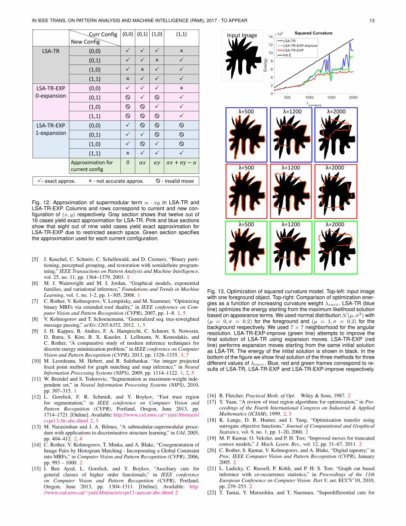
As described in Fig. 2 in each iteration of LSA-TR, eachpairwise supermodular term α · xy is linearized so that theapproximation coincides with the original energy term on currentconfiguration of (x, y) and two out of three remaining configura-tions. The green line in Fig. 12 specifies approximation for eachof four possible current configurations (x, y).This approximationis used to evaluate all possible new configurations. There arefour possible approximations are four possible new configurations,yielding in total 16 cases, see table in Fig. 12, gray section.LSA-TR computes approximation that is exact in twelve out of

sixteen cases. In contrast, during 0-expansion (pink section) or 1-expansion (blue section), only nine out of sixteen cases are validmoves. The advantage of the smaller search space is that the sameapproximation is now accurate in eight out of nine possible cases.

Similarly to other move making algorithms, LSA-TR-EXPstarts with an initial solution and applies a sequence of 0- and 1-expansion until convergence. Each a-expansion is optimized withstandard LSA-TR alg. 1. For simplicity, in a-expansion, we usehard constraint to prevent variables currently labeled with a fromchanging their label. More efficient implementation would excludevariables that are currently labeled with a from optimization.

Below we focus on the squared curvature regularization modelproposed in [37]. The model is defined in terms of n × n neigh-borhood system, where larger n corresponds to higher angularresolution. In combination with appearance terms, the modelyields discrete binary energy that has both submodular and non-submodular pairwise potentials. The weight of curvature termrelative to appearance term is controlled by parameter λcurv. In[37] they show that LSA-TR outperforms all other currently avail-able optimization methods for non-submodular binary energies.Therefore, in this section we only compare LSA-TR with theproposed move making LSA-TR-EXP.

For this application we selected a synthetic image examplewhere foreground object has an osculating contour. We vary theweight λcurv and compare the performance of LSA-TR and LSA-TR-EXP. Figure 13 shows the input image in top-left and thecomparison graph in top right. When the weight of supermodularcurvature terms increases, LSA-TR-EXP (red line) consistentlyoutperforms LSA-TR (blue line) when starting from the sameinitial solution. LSA-TR-EXP-improve (green line) attempts andoften succeeds to improve the final solution of LSA-TR. Theenergy of the initial solution for each λcurv is shown in black.

Figure. 13, bottom shows the final results of the three differentmethods for three different values of λcurv. The red outline withineach image denotes the final solution. Blue, red and green framescorrespond to results of LSA-TR, LSA-TR-EXP and LSA-TR-EXP-improve respectively.

4 OPTIMIZATION LIMITATIONS

The proposed LSA-TR and LSA-AUX methods belong to a moregeneral class of local iterative optimization and therefore can onlyguarantee a local minimum at convergence, see Sec. 2.1 and 2.2.Figure 14 demonstrates some sensitivity with respect to initial-ization. The trivial initialization with all pixels in the foreground,denoted by“init 1” and delineated by the red contour, leads toa poor local minimum. Using the appearance based maximumlikelihood label per pixel as initialization, denoted by “init 2”,results in a much lower optimum. From empirical observations,we obtain better results starting with appearance based maximumlikelihood labels when possible.

5 CONCLUSIONS AND FUTURE WORK

We proposed two specific LSA algorithms based on trust regionand auxiliary function principles. Our methods obtain state-of-the-art results on a wide range of applications that require optimizationof binary non-submodular energies. Our methods outperformmany standard techniques such as LBP, QPBO, and TRWS. Inaddition, we proposed a move-making extension to the LSA-TRapproach. In the future, we plan to explore other variants of movemaking algorithms in combination with LSA.

IN IEEE TRANS. ON PATTERN ANALYSIS AND MACHINE INTELLIGENCE (PAMI), 2017 - TO APPEAR 12

LSA-AUXE=0T=3.38s

LSA-AUXPE=0T=2.86s

IPFPE= -167540T= 105s

LBPE= -309556T= 262s

QPBO3.8% labeled

QPBO-IE= -77752T=55.3s

SRMPE= -316122T=1118s

TRWSE= -184754T=253s

LSA-TRE= -336486T= 31s

Input Img

User Scribbles for Appearance

Appearance Terms

Fig. 11. Compact Shape Prior results and comparison with other methods. The left column shows input image, user scribbles and resultingappearance terms. Red colors show preference to foreground and blue colors show preference to background. The remaining columns show foreach method the final image segmentation along with the corresponding labeling on each of the four layers in the graph. Gray color in QPBO resultsdenotes unlabeled pixels. In the bottom we compare the methods in terms of energy and the running time (shown in log-scale).

We also plan to research additional applications that can bene-fit from efficient optimization of binary non-submodular pairwiseenergies. For instance, our experiments show that our approachcan improve non-submodular α-expansion and fusion moves formultilabel energies.

Moreover, while our paper focuses on pairwise interactions,our approach naturally extends to high-order potentials that appearin computer vision problems. We already successfully appliedLSA to optimization of convexity shape prior [35]. We furtherplan to explore other high-order energies such as visibility andsilhouette consistency in multi-view reconstruction, connectivityshape prior and absolute curvature regularization.

6 ACKNOWLEDGEMENTS

We greatly thank V. Kolmogorov for his feedback. We also thankNSERC and NIH for their grants supporting this project.

REFERENCES

[1] E. Boros and P. L. Hammer, “Pseudo-boolean optimization,” DiscreteApplied Mathematics, vol. 123, p. 2002, 2001. 1, 10

[2] R. Lazimy, “Mixed integer quadratic programming,” Mathematical Pro-gramming, vol. 22, pp. 332–349, 1982. 1

[3] M. Goemans and D. Wiliamson, “Improved approximation algorithmsfor maximum cut and satisfiability problem using semidefinite problem,”ACM, vol. 42, no. 6, pp. 1115–1145, 1995. 1

[4] C. Olsson, A. Eriksson, and F. Kahl, “Improved spectral relaxationmethods for binary quadratic optimization problems,” Comp. Vis. &Image Underst., vol. 112, no. 1, pp. 3–13, 2008. 1, 2

IN IEEE TRANS. ON PATTERN ANALYSIS AND MACHINE INTELLIGENCE (PAMI), 2017 - TO APPEAR 13

- exact approx. - not accurate approx. - invalid move

Curr ConfigNew Config

(0,0) (0,1) (1,0) (1,1)

LSA-TR (0,0)

(0,1)

(1,0)

(1,1)

LSA-TR-EXP0-expansion

(0,0)

(0,1)

(1,0)

(1,1)

LSA-TR-EXP1-expansion

(0,0)

(0,1)

(1,0)

(1,1)

Approximation forcurrent config

0 𝛼𝑥 𝛼𝑦 𝛼𝑥 + 𝛼y − 𝛼

Fig. 12. Approximation of supermodular term α · xy in LSA-TR andLSA-TR-EXP. Columns and rows correspond to current and new con-figuration of (x, y) respectively. Gray section shows that twelve out of16 cases yield exact approximation for LSA-TR. Pink and blue sectionsshow that eight out of nine valid cases yield exact approximation forLSA-TR-EXP due to restricted search space. Green section specifiesthe approximation used for each current configuration.

[5] J. Keuchel, C. Schnorr, C. Schellewald, and D. Cremers, “Binary parti-tioning, perceptual grouping, and restoration with semidefinite program-ming,” IEEE Transactions on Pattern Analysis and Machine Intelligence,vol. 25, no. 11, pp. 1364–1379, 2003. 1

[6] M. J. Wainwright and M. I. Jordan, “Graphical models, exponentialfamilies, and variational inference,” Foundations and Trends in MachineLearning, vol. 1, no. 1-2, pp. 1–305, 2008. 1

[7] C. Rother, V. Kolmogorov, V. Lempitsky, and M. Szummer, “Optimizingbinary MRFs via extended roof duality,” in IEEE conference on Com-puter Vision and Pattern Recognition (CVPR), 2007, pp. 1–8. 1, 5

[8] V. Kolmogorov and T. Schoenemann, “Generalized seq. tree-reweightedmessage passing,” arXiv:1205.6352, 2012. 1, 5

[9] J. H. Kappes, B. Andres, F. A. Hamprecht, C. Schnorr, S. Nowozin,D. Batra, S. Kim, B. X. Kausler, J. Lellmann, N. Komodakis, andC. Rother, “A comparative study of modern inference techniques fordiscrete energy minimization problem,” in IEEE conference on ComputerVision and Pattern Recognition (CVPR), 2013, pp. 1328–1335. 1, 7

[10] M. Leordeanu, M. Hebert, and R. Sukthankar, “An integer projectedfixed point method for graph matching and map inference.” in NeuralInformation Processing Systems (NIPS), 2009, pp. 1114–1122. 1, 2, 5

[11] W. Brendel and S. Todorovic, “Segmentation as maximum-weight inde-pendent set,” in Neural Information Processing Systems (NIPS), 2010,pp. 307–315. 1

[12] L. Gorelick, F. R. Schmidt, and Y. Boykov, “Fast trust regionfor segmentation,” in IEEE conference on Computer Vision andPattern Recognition (CVPR), Portland, Oregon, June 2013, pp.1714–1721. [Online]. Available: http://www.csd.uwo.ca/∼yuri/Abstracts/cvpr13-ftr-abs.shtml 2, 3

[13] M. Narasimhan and J. A. Bilmes, “A submodular-supermodular proce-dure with applications to discriminative structure learning,” in UAI, 2005,pp. 404–412. 2, 4

[14] C. Rother, V. Kolmogorov, T. Minka, and A. Blake, “Cosegmentation ofImage Pairs by Histogram Matching - Incorporating a Global Constraintinto MRFs,” in Computer Vision and Pattern Recognition (CVPR), 2006,pp. 993 – 1000. 2

[15] I. Ben Ayed, L. Gorelick, and Y. Boykov, “Auxiliary cuts forgeneral classes of higher order functionals,” in IEEE conferenceon Computer Vision and Pattern Recognition (CVPR), Portland,Oregon, June 2013, pp. 1304–1311. [Online]. Available: http://www.csd.uwo.ca/∼yuri/Abstracts/cvpr13-auxcut-abs.shtml 2

Input Image

λ=500

λ=1200

λ=1200

λ=1200λ=500

λ=500 λ=2000

λ=2000

λ=2000λ=2000

Fig. 13. Optimization of squared curvature model. Top-left: input imagewith one foreground object. Top-right: Comparison of optimization ener-gies as a function of increasing curvature weight λcurv . LSA-TR (blueline) optimizes the energy starting from the maximum likelihood solutionbased on appearance terms. We used normal distributionN (µ, σ2) with(µ = 0, σ = 0.2) for the foreground and (µ = 1, σ = 0.2) for thebackground respectively. We used 7 × 7 neighborhood for the angularresolution. LSA-TR-EXP-improve (green line) attempts to improve thefinal solution of LSA-TR using expansion moves. LSA-TR-EXP (redline) performs expansion moves starting from the same initial solutionas LSA-TR. The energy of the initial solution is shown in black. In thebottom of the figure we show final solution of the three methods for threedifferent values of λcurv . Blue, red and green frames correspond to re-sults of LSA-TR, LSA-TR-EXP and LSA-TR-EXP-improve respectively.

[16] R. Fletcher, Practical Meth. of Opt. Wiley & Sons, 1987. 2[17] Y. Yuan, “A review of trust region algorithms for optimization,” in Pro-

ceedings of the Fourth International Congress on Industrial & AppliedMathematics (ICIAM), 1999. 2, 3

[18] K. Lange, D. R. Hunter, and I. Yang, “Optimization transfer usingsurrogate objective functions,” Journal of Computational and GraphicalStatistics, vol. 9, no. 1, pp. 1–20, 2000. 2

[19] M. P. Kumar, O. Veksler, and P. H. Torr, “Improved moves for truncatedconvex models,” J. Mach. Learn. Res., vol. 12, pp. 31–67, 2011. 2

[20] C. Rother, S. Kumar, V. Kolmogorov, and A. Blake, “Digital tapestry,” inProc. IEEE Computer Vision and Pattern Recognition (CVPR), January2005. 2

[21] L. Ladicky, C. Russell, P. Kohli, and P. H. S. Torr, “Graph cut basedinference with co-occurrence statistics,” in Proceedings of the 11thEuropean Conference on Computer Vision: Part V, ser. ECCV’10, 2010,pp. 239–253. 2

[22] T. Taniai, Y. Matsushita, and T. Naemura, “Superdifferential cuts for

IN IEEE TRANS. ON PATTERN ANALYSIS AND MACHINE INTELLIGENCE (PAMI), 2017 - TO APPEAR 14

E=62491 E=56028 E=56028

LSA-TR LSA-TR-EXP improve LSA-TR-EXP LSA-AUX

E=250618

E=38576 E=35210 E=31368 E=33412

Init 1

E=250618

E=67540

Init 2

Fig. 14. Local optimization of squared curvature might yield differentsegmentation results for different initializations. First row - starting withall pixels assigned to foreground, second row - starting with appearancebased ML labeling. Here we used λcurv = 1000.

binary energies,” in IEEE Conference on Computer Vision and PatternRecognition, CVPR 2015, Boston, MA, USA, June 7-12, 2015, 2015, pp.2030–2038. 2

[23] M. Tang, I. B. Ayed, and Y. Boykov, “Pseudo-bound optimization forbinary energies,” in Computer Vision - ECCV 2014 - 13th EuropeanConference, Zurich, Switzerland, September 6-12, 2014, Proceedings,Part V, 2014, pp. 691–707. 2

[24] Y. Boykov, V. Kolmogorov, D. Cremers, and A. Delong, “An integralsolution to surface evolution PDEs via Geo-Cuts,” in European Conf. onComp. Vision (ECCV), 2006. 3

[25] J. Ulen, P. Strandmark, and F. Kahl, “An efficient optimization frame-work for multi-region segmentation based on Lagrangian duality,” IEEETransactions on Medical Imaging, vol. 32, no. 2, pp. 178–188, 2013. 3

[26] Y. Boykov, V. Kolmogorov, D. Cremers, and A. Delong, “An IntegralSolution to Surface Evolution PDEs via Geo-Cuts,” ECCV, LNCS 3953,vol. 3, pp. 409–422, May 2006. 3

[27] J. Pearl, “Reverend bayes on inference engines: A distributed hierarchicalapproach,” in National Conference on Artificial Intelligence, 1982, pp.133–136. 5

[28] N. El-Zehiry and L. Grady, “Fast global optimization of curvature,” inIEEE conference on Computer Vision and Pattern Recognition (CVPR),no. 3257-3264, 2010. 6, 7, 8

[29] N. Bansal, A. Blum, and S. Chawla, “Correlation clustering,” in MachineLearning, vol. 56, no. 1-3, 2004, pp. 89–113. 6

[30] J. H. Kappes, M. Speth, G. Reinelt, and C. Schnorr, “Higher-ordersegmentation via multicuts,” Comput. Vis. Image Underst., vol. 143,no. C, pp. 104–119, Feb. 2016. 6

[31] Y. Boykov and M.-P. Jolly, “Interactive graph cuts for optimal boundaryand region segmentation of objects in n-d images,” in IEEE InternationalConference on Computer Vision (ICCV), no. 105-112, 2001. 6

[32] A. Delong and Y. Boykov, “Globally optimal segmentation of multi-region objects,” in IEEE 12th International Conference on ComputerVision, ICCV 2009, Kyoto, Japan, September 27 - October 4, 2009, 2009,pp. 285–292. 7

[33] P. Das, O. Veksler, V. Zavadsky, and Y. Boykov, “Semiautomatic seg-mentation with compact shape prior,” Image Vision Computing, vol. 27,no. 1-2, pp. 206–219, 2009. 9, 11

[34] D. Schlesinger, “Exact solution of permuted submodular minsum prob-lems,” in Energy Minimization Methods in Computer Vision and PatternRecognition, 6th International Conference, EMMCVPR 2007, Ezhou,China, August 27-29, 2007, Proceedings, 2007, pp. 28–38. 10

[35] L. Gorelick, O. Veksler, Y. Boykov, and C. Nieuwenhuis, “Convexityshape prior for segmentation,” in Computer Vision - ECCV 2014 -13th European Conference, Zurich, Switzerland, September 6-12, 2014,Proceedings, Part V, 2014, pp. 675–690. 10, 12

[36] Y. Boykov, O. Veksler, and R. Zabih, “Fast approximate energy mini-mization via graph cuts,” IEEE Trans. Pattern Anal. Mach. Intell., vol. 23,no. 11, pp. 1222–1239, 2001. 11

[37] C. Nieuwenhuis, E. Toppe, L. Gorelick, O. Veksler, and Y. Boykov,“Efficient squared curvature,” in 2014 IEEE Conference on ComputerVision and Pattern Recognition, CVPR 2014, Columbus, OH, USA, June23-28, 2014, 2014, pp. 4098–4105. 11

Lena Gorelick received the BSc degree cumlaude in computer science from Bar-Ilan Univer-sity in 2001, the MSc degree summa cum laudein computer science and applied mathematicsfrom the Weizmann Institute of Science in 2004and PhD degree in computer science and ap-plied mathematics from the Weizmann Instituteof Science in 2009. From 2009 to 2014 shewas a postdoctoral fellow at computer sciencedepartment of the University of Western Ontarioand since 2014 she is a research scientist there.

Her current research interests lie in computer vision, specifically inthe area of shape analysis, image segmentation and discrete energyminimization methods.

Olga Veksler received BS degree in mathemat-ics and computer science from New York Uni-versity in 1995 and a PhD degree from CornellUniversity in 1999. She was a postdoctoral as-sociate at NEC Research Institute. She is cur-rently a full professor with Computer Science De-partment University of Western Ontario. Her re-search interests are energy minimization meth-ods, graph algorithms, stereo correspondence,motion, and segmentation. She is a receiver ofthe early researcher award from Ontario Ministry

of Research and Innovation, NSERC-DAS award, and Helmholtz Prize(Test of Time) awarded at the International Conference on ComputerVision, 2011.

Yuri Boykov received ”Diploma of Higher Ed-ucation” with honors at Moscow Institute ofPhysics and Technology in 1992 and completedhis Ph.D. at the department of Operations Re-search at Cornell University in 1996. He is cur-rently a full professor at the department of Com-puter Science at the University of Western On-tario. His research is concentrated in the area ofcomputer vision and biomedical image analysis.In particular, he is interested in problems of earlyvision, image segmentation, restoration, regis-

tration, stereo, motion, model fitting, feature-based object recognition,photo-video editing and others. He is a recipient of the Helmholtz Prize(Test of Time) awarded at International Conference on Computer Vision(ICCV), 2011 and Florence Bucke Science Award, Faculty of Science,The University of Western Ontario, 2008.

Andrew Delong received the B.Math. degreein computer science from the University of Wa-terloo in 2003 and the M.Sc. and Ph.D. degreein computer science from Western University in2006 and 2011, respectively. He is a Postdoc-toral Fellow at the University of Toronto. Prior toentering academia he worked in the computergraphics industry. His research interests includemachine learning, computer vision, combinato-rial optimization, and computational biology. Dr.Delong was awarded a NSERC Postgraduate

Scholarship, an NSERC Postdoctoral Fellowship, a Heffernan Commer-cialization Fellowship, and a 2016 Invention of the Year Award from theUniversity of Toronto.

Ismail Ben Ayed received the PhD degree (withthe highest honor) in computer vision from theINRS-EMT, Montreal in 2007. He is currentlyan Associate Professor at the TS, University ofQuebec. Before joining the TS, he worked for 8years as a research scientist at GE Healthcare,London, ON. He also holds an adjunct professorappointment at Western University (since 2012).Ismails research interests include computer vi-sion, optimization, machine learning and theirpotential applications in medical image analysis.

He co-authored a book, over seventy peer-reviewed publications, mostlypublished in the top venues in these subject areas, and six US patents.