Local sourcing and production efficiency

Local sourcing and production efficiency

Emmanuel Dhyne (BNB, UMONS)Cédric Duprez (BNB)

Séminaire Fourgeaud, Ministère de l’Économie, Paris, 7 juin 2017

Disclaimer : The views expressed are those of the authors and do not

necessarily reflect the views of the National Bank of Belgium. The statistical

evidence presented complies with the Belgian legislation on statistical secrecy.

Presentation2 / xx

Structure

► Motivation

► A model of local and global sourcing

► The Belgian production network

► Bringing the model to the data

● Using individual transactions data

● Using firm x province data

● Using firm data

► Concluding remarks

Presentation3 / xx

Motivation

► Reduction in trade costs + ICT revolution has totally alter the organization of

production within firms

► => increased fragmentation of production process

► Old model : (Almost) all the tasks required to produce a final good (design,

production, supporting activities) were done in house

► New model : Each firm focuses on its core abilities and outsource / offshore

its non core activities

► Global Value Chains : well documented phenomenon in the international

trade literature + well-know examples (Apple, Airbus)

► Local Value Chains : less documented, mostly because of lack of data but…

► … 84% of trade in intermediaries are domestic trade

Presentation4 / xx

Efficiency gains drives the local / global fragmentation

of the production process

Presentation5 / xx

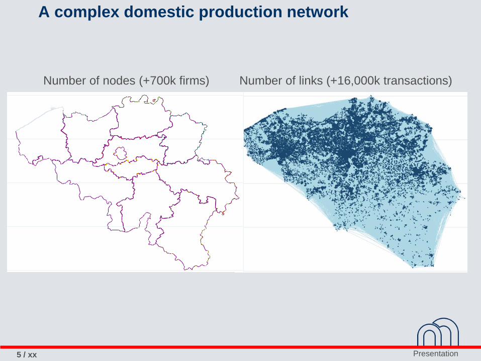
Number of nodes (+700k firms) Number of links (+16,000k transactions)

A complex domestic production network

49

.550

50

.551

51

.5

2 3 4 5 6

Presentation6 / xx

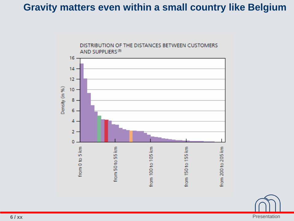
Gravity matters even within a small country like Belgium

Presentation7 / xx

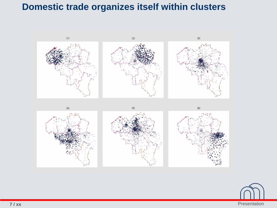
Domestic trade organizes itself within clusters

Presentation8 / xx

Related literature

► Determinants of foreign sourcing

● Amiti and Konings (2007), Golberg et al., (2010), Halpern et al. (2015),

Bøler et al., (2015), Antràs, Fort and Tintelnot (2017)

► Determinants of local sourcing

● Bernard et al., (2015), Furusawa et al., (2017)

► Organization of production network

● Oberfield (2013)

► Characterization of the production chain

● Antràs et al. (2012), Fally (2011)

Presentation9 / xx

Structure

► Motivation






● Using firm data


Presentation10 / xx

A model of local and global sourcing

► Adaptation of AFT (2017) multi-country sourcing model at a local level

► Model with firms producing final goods by aggregating intermediate tasks

► Firms do not trade intermediate goods but tasks

► Main driver of inter-firm trade : heterogeneity in the ability to perform a

subset of tasks

► Tasks can be traded locally and internationally

► Trade in tasks entails fixed and variable costs

Presentation11 / xx

Ex: Why do some bakers only bake and some only sell ?

► Final product : Bread

► Tasks required to sell bread to final consumer :

● (1) Conception and R&D : development of a new recipe + design of the bread loaf

● (2) Sowing, growing and harvesting the wheat

● (3) Milling the wheat

● (4) Mixing the flour with water (endowment)

● (5) Baking the bread

● (6) Selling the bread

● (7) + book-keeping, marketing, finance (customer credit),….

► The baker’s abilities are in tasks (4) and (5) and potentially in (1) and (6).

Outsourcing tasks (2), (3) and (7) may raise profits,

► Extreme case : Only good in (6), outsourcing all other tasks

Presentation12 / xx

Set-up

► Preferences are CES. Demand in country c for variety 𝜔 is

𝑞𝑐 𝜔 = 𝐸𝑐 𝑃𝑐 𝜎−1𝑝𝑐 𝜔 −𝜎

► Monopolistic competition. Each firm owns a blueprint to produce a single

variety 𝜔

► Production requires the assembly of a unit continuum of tasks. Marginal cost

of firm i is

𝑐𝑖 = 01𝑧𝑖 𝑡

1−𝜌𝑑𝑡1/(1−𝜌)

where zi(t) is the price of an individual task t paid by firm i

Presentation13 / xx

Set-up

► Firms draw all their unit labor requirements associated with task t, 𝑎𝑖 𝑡 , from

the Frechet distribution (EK, 2002)

𝑃𝑟 𝑎𝑖 𝑡 ≥ 𝑎 = 𝑒−𝛾𝑖𝑎𝜃

► 𝛾𝑖, the ability to manage tasks, is the source of firm heterogeneity (cf. Bloom et

al., 2017, Syverson, 2011)

► All firms can produce all tasks in-house, or they can concentrate on their core

(good draws) tasks and outsource the remaining tasks

► Outsourcing entails fixed (fij) and variable costs (𝜏𝑖𝑗) 𝑧𝑖 𝑡 =

min𝑗∈𝐽𝑖

𝜏𝑖𝑗𝑎𝑗 𝑡 𝑤𝑗

with Ji the set of firms (including i) for which i has paid the fixed cost fij (fii=0)

Presentation14 / xx

Optimal sourcing strategy

► From Frechet distribution, the share of tasks sourced from any supplier j is

𝑋𝑖𝑗 =𝛾𝑗 𝜏𝑖𝑗𝑤𝑗

−𝜃

Θ𝑖with sourcing strategy Θ𝑖 = 𝑘∈𝐽𝑖 𝛾𝑘 𝜏𝑖𝑘𝑤𝑘

−𝜃 (AFT, 2017)

► Using the properties of the Frechet and constant mark-up, firms’ profit is

Max𝐼𝑖𝑗∈ 0,1

𝑗 𝐼𝑖𝑗𝛾𝑗 𝜏𝑖𝑗𝑤𝑗−𝜃 𝜎−1 /𝜃

𝐵𝑖 − 𝑤𝑖 𝑗 𝐼𝑖𝑗𝐹𝑖𝑗

► If 𝜎 − 1 > 𝜃, sourcing exhibits complementarities. The marginal gain from

adding a new supplier increases with the addition of other suppliers.

Presentation15 / xx

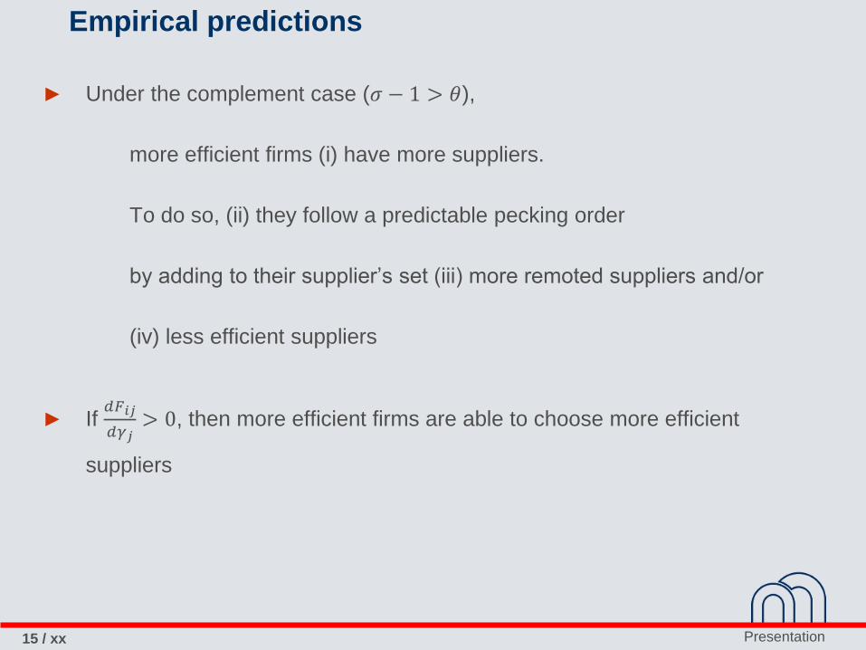
Empirical predictions

► Under the complement case (𝜎 − 1 > 𝜃),

more efficient firms (i) have more suppliers.

To do so, (ii) they follow a predictable pecking order

by adding to their supplier’s set (iii) more remoted suppliers and/or

(iv) less efficient suppliers

► If 𝑑𝐹𝑖𝑗

𝑑𝛾𝑗> 0, then more efficient firms are able to choose more efficient

suppliers

Presentation16 / xx

Structure

► Motivation






● Using firm data


Presentation17 / xx

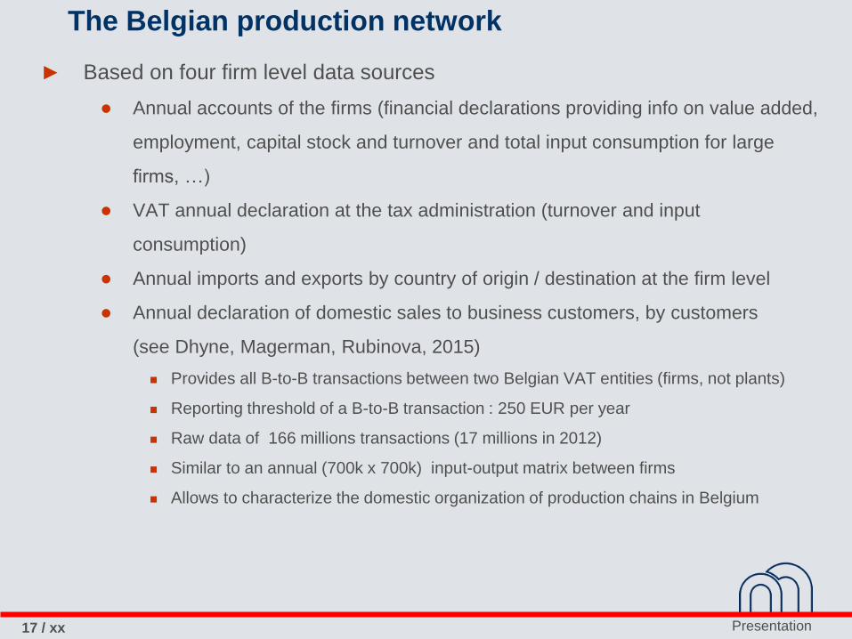
The Belgian production network

► Based on four firm level data sources

● Annual accounts of the firms (financial declarations providing info on value added,

employment, capital stock and turnover and total input consumption for large

firms, …)

● VAT annual declaration at the tax administration (turnover and input

consumption)

● Annual imports and exports by country of origin / destination at the firm level

● Annual declaration of domestic sales to business customers, by customers

(see Dhyne, Magerman, Rubinova, 2015)

Provides all B-to-B transactions between two Belgian VAT entities (firms, not plants)

Reporting threshold of a B-to-B transaction : 250 EUR per year

Raw data of 166 millions transactions (17 millions in 2012)

Similar to an annual (700k x 700k) input-output matrix between firms

Allows to characterize the domestic organization of production chains in Belgium

Presentation18 / xx

The sourcing strategies of Belgian firms

Descriptive statistics - Sourcing strategies in 2012

Note : Sample size = 797,596 Belgian firms

p10 p25 p50 p75 p90 Mean

Number of domestic suppliers 1 4 9 23 47 21.2

Share of importers (in %) - - - - - 5.1

Number of sourcing foreign countries

(conditional on international sourcing) 1 1 2 4 9 3,8

Presentation19 / xx

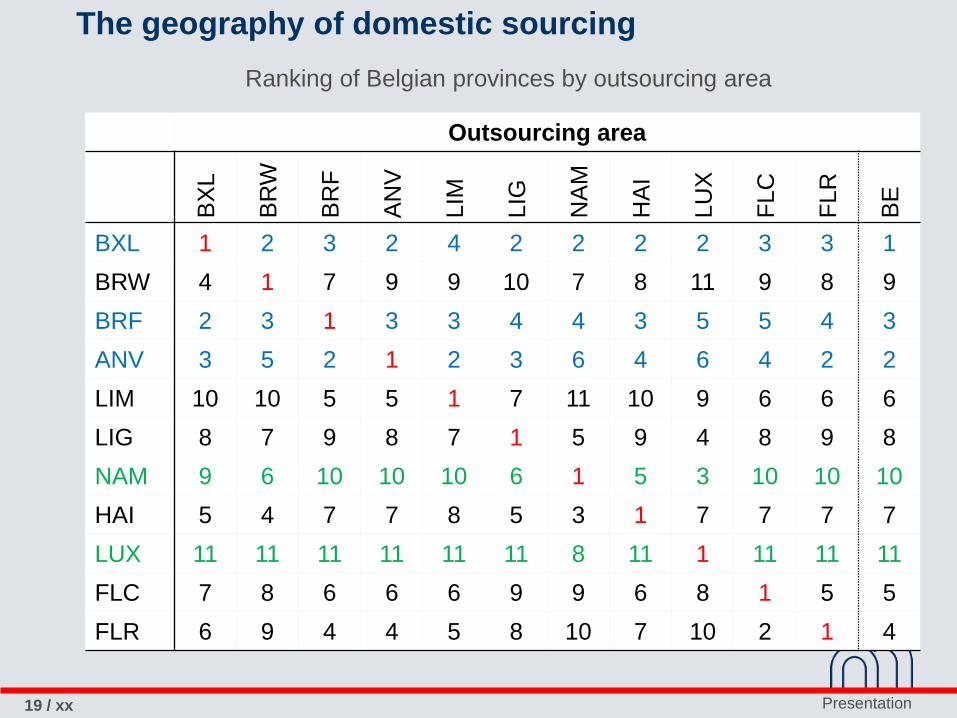
The geography of domestic sourcing

Ranking of Belgian provinces by outsourcing area

Outsourcing area

BX

L

BR

W

BR

F

AN

V

LIM

LIG

NA

M

HA

I

LU

X

FLC

FLR

BE

BXL 1 2 3 2 4 2 2 2 2 3 3 1

BRW 4 1 7 9 9 10 7 8 11 9 8 9

BRF 2 3 1 3 3 4 4 3 5 5 4 3

ANV 3 5 2 1 2 3 6 4 6 4 2 2

LIM 10 10 5 5 1 7 11 10 9 6 6 6

LIG 8 7 9 8 7 1 5 9 4 8 9 8

NAM 9 6 10 10 10 6 1 5 3 10 10 10

HAI 5 4 7 7 8 5 3 1 7 7 7 7

LUX 11 11 11 11 11 11 8 11 1 11 11 11

FLC 7 8 6 6 6 9 9 6 8 1 5 5

FLR 6 9 4 4 5 8 10 7 10 2 1 4

Presentation20 / xx

Peaking order of sourcing area is not random

Presentation21 / xx

Structure

► Motivation






● Using firm data


Presentation22 / xx

Using individual transactions data

► Estimation of Heckit model

● Heckman 1st stage : Probit equation of a transaction between i (buyer) and j (supplier)

● Heckman 2nd stage : Amount traded between i and j, conditional on selection

► Use only one cross section for 2012

► Similar results obtained for other cross-sections

► 1st stage equation :

● we observe all the “1”s (5,023,543 transactions with explanatory variables), involving

110,129 firms, but too many “0”s (12,123,262,969 potential transactions)

● Random selection of 8,659,331 “0”s + weighting Probit

● Selection variable : i and j belong to the same sub-network

Presentation23 / xx

Why does i outsource some tasks to j ?

(1) The equation also include two sets sectoral dummies, the first one for firm i and the second for supplier j, two sets

of dummies identifying in which sub-network i or j belong and dummies for the degree of internationalization of i or j

(exporter, importer, MNE). Clustered standard errors by firms are in brackets. *** means significant at the 1% level.

Average Marginal Effects are multiplied by 1,000. (2) Inverse hyperbolic sin of the “as the crow fly” distance between

firm i and supplier j . (3) Total factor productivity, in log, estimated using the Wooldridge LP method.

Presentation24 / xx

How much does i outsource to j ?

(1) The equation also include two sets sectoral dummies, the first one for firm j and the second for supplier i and

dummies for the degree of internationalization of i or j (exporter, importer, MNE). Clustered standard errors by firms

are in brackets. *** means significant at the 1% level. (2) Inverse hyperbolic sin of the “as the crow fly” distance

between supplier j and firm i. (3) Employment in full time equivalent, in log. (4) Total factor productivity, in log,

estimated using the Wooldridge LP method.

Presentation25 / xx

Structure

► Motivation






● Using firm data


Presentation26 / xx

Using firm x province level data

► Aggregating transactions at the province level for either the suppliers or the

customers

► Number of suppliers of firm i by province

► Number of customers of firm i by province

► Unbalanced panel of firms observed between 2002 and 2012

Presentation27 / xx

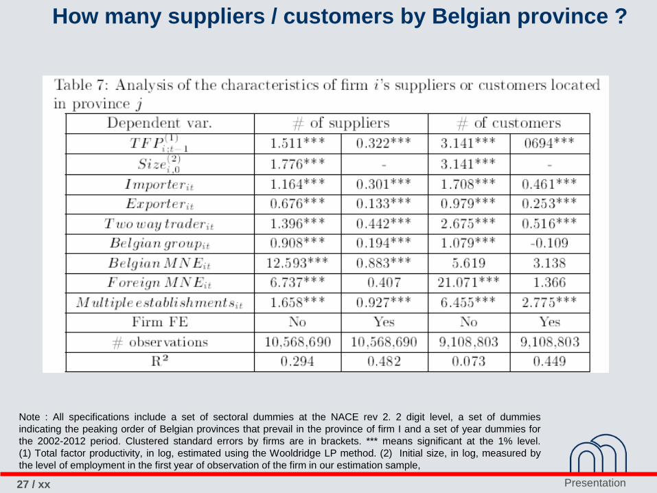
How many suppliers / customers by Belgian province ?

Note : All specifications include a set of sectoral dummies at the NACE rev 2. 2 digit level, a set of dummies

indicating the peaking order of Belgian provinces that prevail in the province of firm I and a set of year dummies for

the 2002-2012 period. Clustered standard errors by firms are in brackets. *** means significant at the 1% level.

(1) Total factor productivity, in log, estimated using the Wooldridge LP method. (2) Initial size, in log, measured by

the level of employment in the first year of observation of the firm in our estimation sample,

Presentation28 / xx

Structure

► Motivation






● Using firm data


Presentation29 / xx

Using firm level data

► Aggregating at the firm level data allows to analyze the characteristics of the

suppliers of firm i

► Maximum distance between i and one of its suppliers

► TFP of the least efficient supplier

► TFP of the most efficient supplier

► Unbalanced panel of firms from 2002 to 2012

Presentation30 / xx

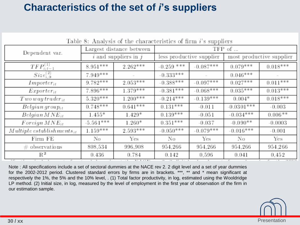
Characteristics of the set of i’s suppliers

Note : All specifications include a set of sectoral dummies at the NACE rev 2. 2 digit level and a set of year dummies

for the 2002-2012 period. Clustered standard errors by firms are in brackets. ***, ** and * mean significant at

respectively the 1%, the 5% and the 10% level, . (1) Total factor productivity, in log, estimated using the Wooldridge

LP method. (2) Initial size, in log, measured by the level of employment in the first year of observation of the firm in

our estimation sample.

Presentation31 / xx

How large is the fixed cost to outsource from j ?

► To assess the importance of the fixed cost associated to source from a

specific supplier, we compare

► j’s rank in terms of number of business customers

► j’s rank in terms of total deliveries

► Firms with few (many) customers but high (low) total sales may be

characterized by high (low) fixed cost

Presentation32 / xx

How large is the fixed cost to outsource from j ?

Note : The dependant variable is the log difference. All specifications include a set of sectoral dummies at the NACE

rev 2. 2 digit level, a set of geographical dummies at the zip code level and a set of year dummies for the 2002-2012

period. Clustered standard errors by firms are in brackets. *** means significant at the 1% level, ** at the 5% level.

(1) Total factor productivity, in log, estimated using the Wooldridge LP method. (2) Initial size, in log, measured by

the level of employment in the first year of observation of the firm in our estimation sample,

Presentation33 / xx

Structure

► Motivation






● Using firm data


Presentation34 / xx

Tentative conclusions (1)

► In this paper, we present a model of local and global sourcing of intermediate

tasks and confront its main prediction to the Belgian production network

► We find that even at the national level, outsourcing decisions are strongly

influenced by geography

► Firms tend to source mostly locally

► Most efficient firms are able to source from more suppliers, located in more

distant places, being either very efficient (high fixed costs) or marginally less

efficient.

► They tend to source more from closer or more productive areas.

Presentation35 / xx

Tentative conclusions (2)

► The fixed costs of sourcing tasks from a given firm is increasing in its…

● TFP

● Size

► Firms that own multiple plants have a lower fixed trade cost

► Importers are also cheaper sourcing partners.

Presentation37 / xx

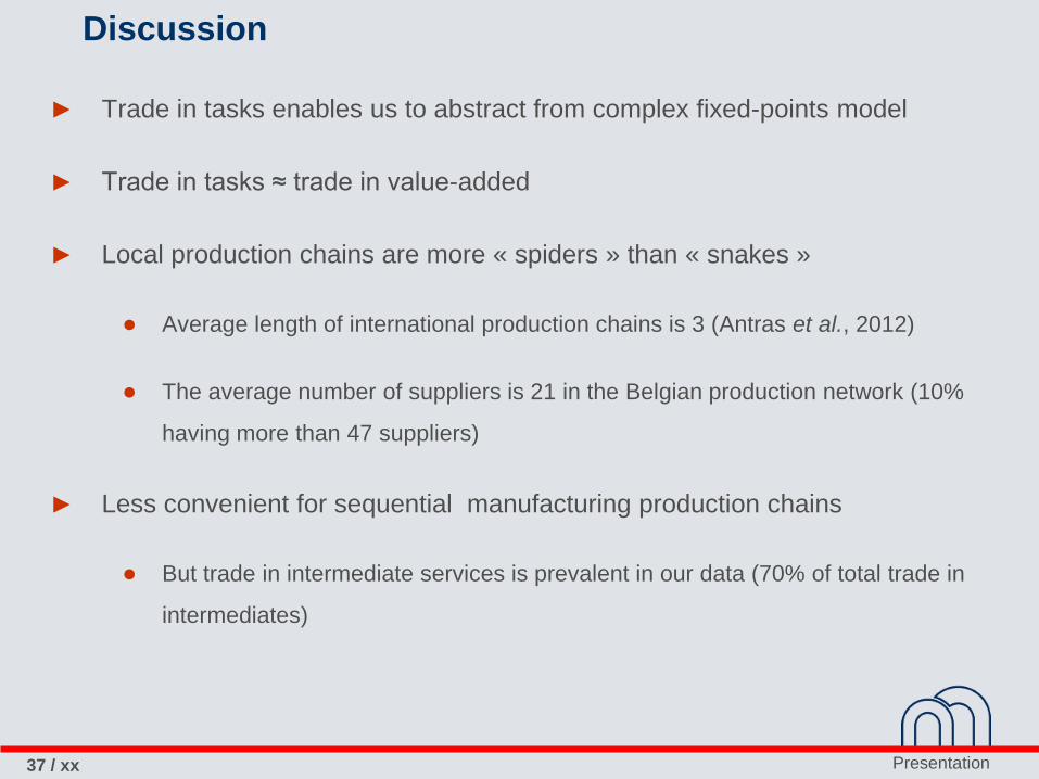
Discussion

► Trade in tasks enables us to abstract from complex fixed-points model

► Trade in tasks ≈ trade in value-added

► Local production chains are more « spiders » than « snakes »

● Average length of international production chains is 3 (Antras et al., 2012)

● The average number of suppliers is 21 in the Belgian production network (10%

having more than 47 suppliers)

► Less convenient for sequential manufacturing production chains

● But trade in intermediate services is prevalent in our data (70% of total trade in

intermediates)

Local sourcing and production efficiency

Documents

Transcript of Local sourcing and production efficiency