Local Search and OptimizationChapter 4

Mausam

(Based on slides of Padhraic Smyth, Stuart Russell, Rao Kambhampati,

Raj Rao, Dan Weld…)

1

2

Outline

• Local search techniques and optimization

– Hill-climbing

– Gradient methods

– Simulated annealing

– Genetic algorithms

– Issues with local search

3

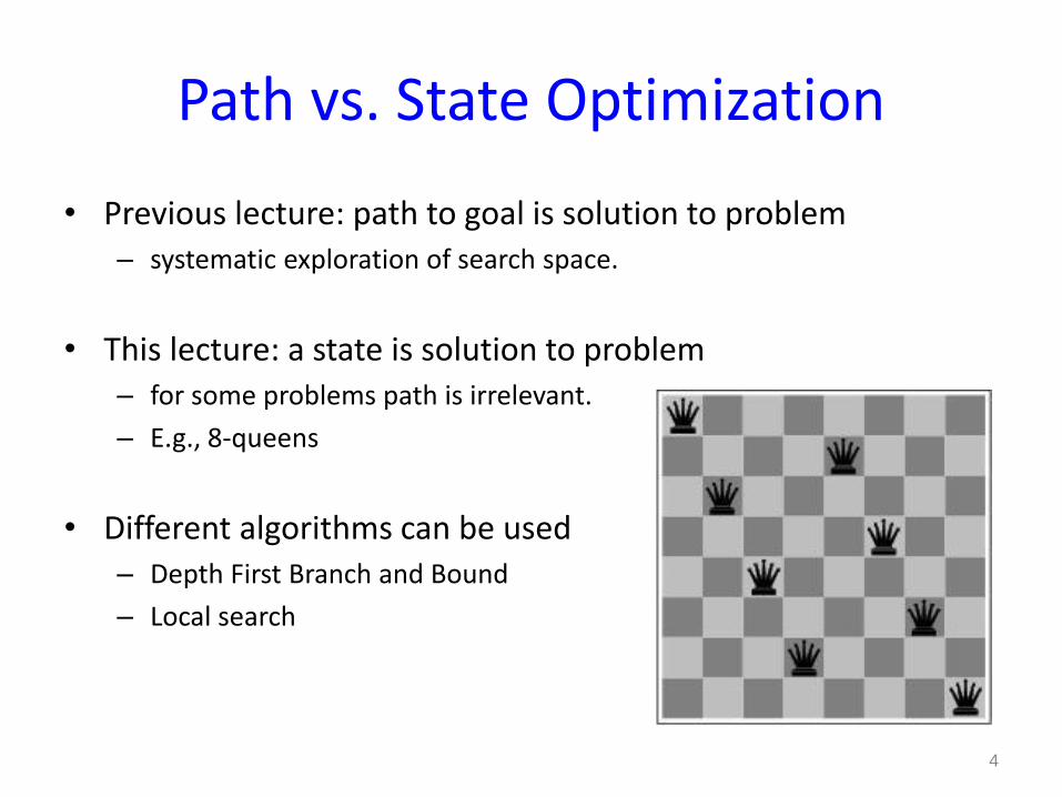
Path vs. State Optimization

• Previous lecture: path to goal is solution to problem– systematic exploration of search space.

• This lecture: a state is solution to problem– for some problems path is irrelevant.

– E.g., 8-queens

• Different algorithms can be used– Depth First Branch and Bound

– Local search

4

Goal Satisfaction

Optimization

reach the goal node

Constraint satisfaction

optimize(objective fn)

Constraint Optimization

You can go back and forth between the two problems

Typically in the same complexity class

© Mausam 5

Satisfaction vs. Optimization

Local search and optimization• Local search

– Keep track of single current state

– Move only to neighboring states

– Ignore paths

• Advantages:– Use very little memory

– Can often find reasonable solutions in large or infinite (continuous) state spaces.

• “Pure optimization” problems– All states have an objective function

– Goal is to find state with max (or min) objective value

– Does not quite fit into path-cost/goal-state formulation

– Local search can do quite well on these problems.

6

Example: n-queens

• Put n queens on an n x n board with no two queens on the same row, column, or diagonal

• Is it a satisfaction problem or optimization?

7

Hill-climbing search: 8-queens problem

• Need to convert to an optimization problem• h = number of pairs of queens that are attacking each other• h = 17 for the above state

8

Search Space

• State

– All 8 queens on the board in some configuration

• Successor function

– move a single queen to another square in the same column.

• Example of a heuristic function h(n):

– the number of pairs of queens that are attacking each other

– (so we want to minimize this) 9

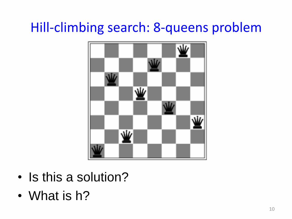
Hill-climbing search: 8-queens problem

• Is this a solution?

• What is h?10

Trivial Algorithms

• Random Sampling

– Generate a state randomly

• Random Walk

– Randomly pick a neighbor of the current state

• Both algorithms asymptotically complete.

© Mausam 11

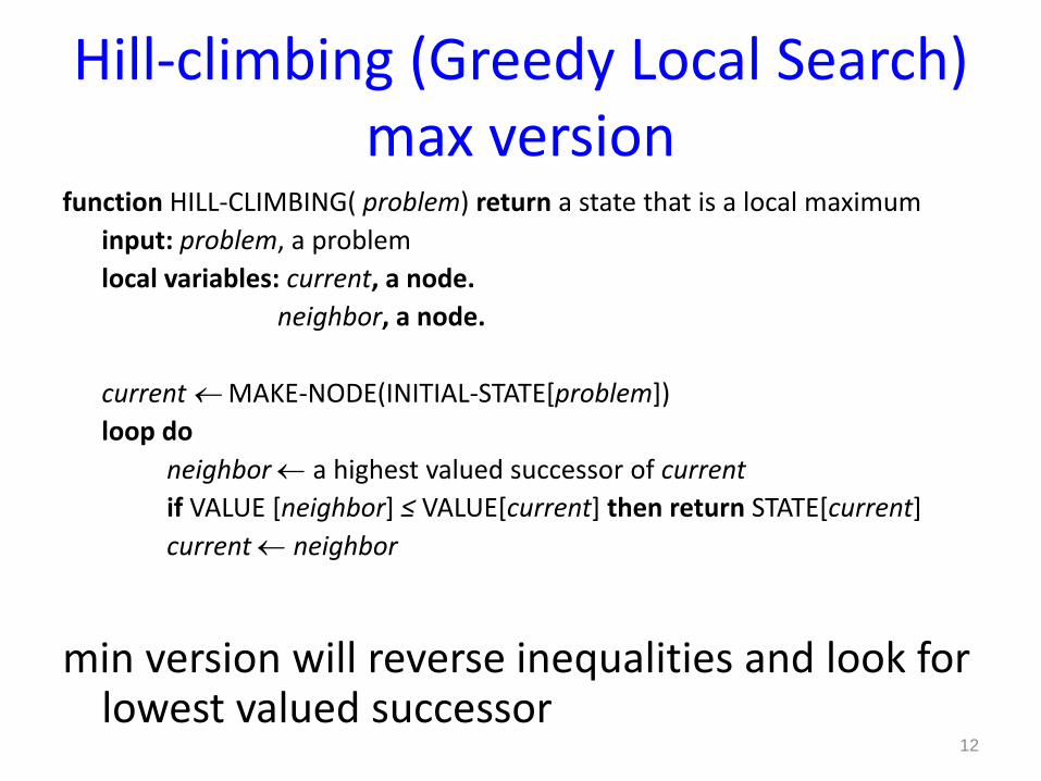
Hill-climbing (Greedy Local Search)max version

function HILL-CLIMBING( problem) return a state that is a local maximum

input: problem, a problem

local variables: current, a node.

neighbor, a node.

current MAKE-NODE(INITIAL-STATE[problem])

loop do

neighbor a highest valued successor of current

if VALUE [neighbor] ≤ VALUE[current] then return STATE[current]

current neighbor

min version will reverse inequalities and look for lowest valued successor

12

Hill-climbing search

• “a loop that continuously moves towards increasing value”– terminates when a peak is reached

– Aka greedy local search

• Value can be either– Objective function value

– Heuristic function value (minimized)

• Hill climbing does not look ahead of the immediate neighbors

• Can randomly choose among the set of best successors – if multiple have the best value

• “climbing Mount Everest in a thick fog with amnesia”

13

“Landscape” of search

Hill Climbing gets stuck in local minima

depending on?

14

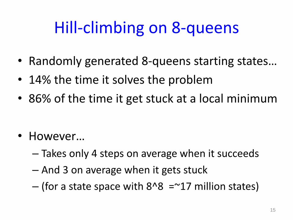
Hill-climbing on 8-queens

• Randomly generated 8-queens starting states…

• 14% the time it solves the problem

• 86% of the time it get stuck at a local minimum

• However…

– Takes only 4 steps on average when it succeeds

– And 3 on average when it gets stuck

– (for a state space with 8^8 =~17 million states)

15

16

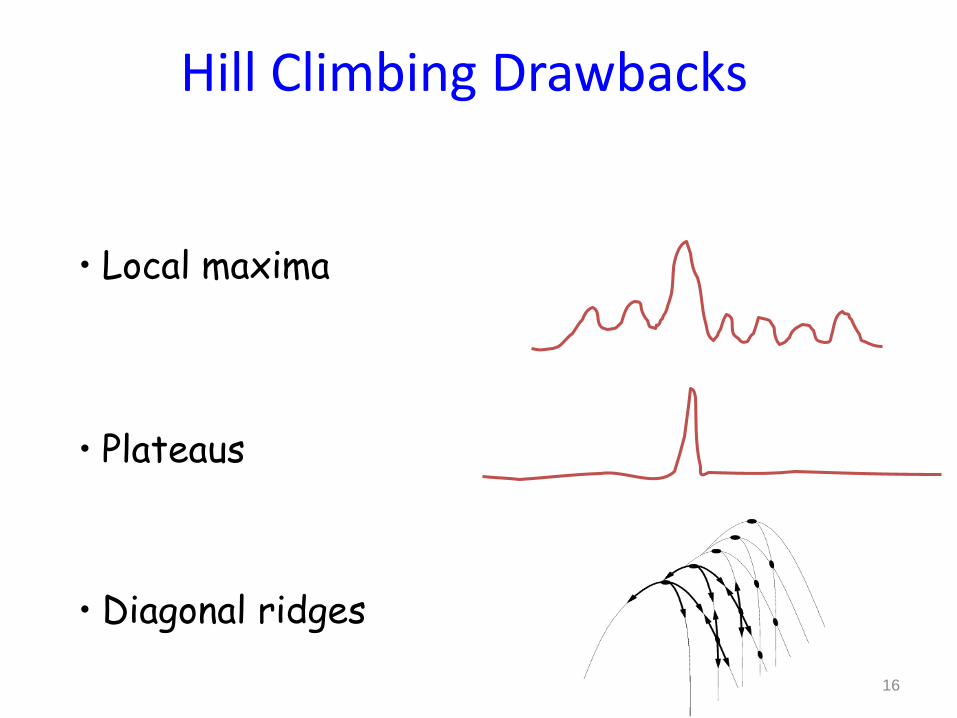
Hill Climbing Drawbacks

• Local maxima

• Plateaus

• Diagonal ridges

Escaping Shoulders: Sideways Move

• If no downhill (uphill) moves, allow sideways moves in hope that algorithm can escape

– Need to place a limit on the possible number of sideways moves to avoid infinite loops

• For 8-queens

– Now allow sideways moves with a limit of 100

– Raises percentage of problem instances solved from 14 to 94%

– However….• 21 steps for every successful solution

• 64 for each failure17

Tabu Search

• prevent returning quickly to the same state

• Keep fixed length queue (“tabu list”)

• add most recent state to queue; drop oldest

• Never make the step that is currently tabu’ed

• Properties:

– As the size of the tabu list grows, hill-climbing will asymptotically become “non-redundant” (won’t look at the same state twice)

– In practice, a reasonable sized tabu list (say 100 or so) improves the performance of hill climbing in many problems18

Escaping Shoulders/local OptimaEnforced Hill Climbing

• Perform breadth first search from a local optima

– to find the next state with better h function

• Typically,

– prolonged periods of exhaustive search

– bridged by relatively quick periods of hill-climbing

• Middle ground b/w local and systematic search

© Mausam 19

Hill-climbing: stochastic variations

• Stochastic hill-climbing– Random selection among the uphill moves.

– The selection probability can vary with the steepness of the uphill move.

• To avoid getting stuck in local minima– Random-walk hill-climbing

– Random-restart hill-climbing

– Hill-climbing with both

20

Hill Climbing with random walk

When the state-space landscape has local minima, any search that moves only in the greedy direction cannot be complete

Random walk, on the other hand, is

asymptotically complete

Idea: Put random walk into greedy hill-climbing

• At each step do one of the two

– Greedy: With prob p move to the neighbor with largest value

– Random: With prob 1-p move to a random neighbor 21

Hill-climbing with random restarts

• If at first you don’t succeed, try, try again!

• Different variations

– For each restart: run until termination vs. run for a fixed time

– Run a fixed number of restarts or run indefinitely

• Analysis

– Say each search has probability p of success• E.g., for 8-queens, p = 0.14 with no sideways moves

– Expected number of restarts?

– Expected number of steps taken?

• If you want to pick one local search algorithm, learn this one!!22

Hill-climbing with both

• At each step do one of the three

– Greedy: move to the neighbor with largest value

– Random Walk: move to a random neighbor

– Random Restart: Resample a new current state

23

Simulated Annealing

• Simulated Annealing = physics inspired twist on random walk

• Basic ideas:– like hill-climbing identify the quality of the local improvements

– instead of picking the best move, pick one randomly

– say the change in objective function is d

– if d is positive, then move to that state

– otherwise:

• move to this state with probability proportional to d

• thus: worse moves (very large negative d) are executed less often

– however, there is always a chance of escaping from local maxima

– over time, make it less likely to accept locally bad moves

– (Can also make the size of the move random as well, i.e., allow “large” steps in state space)

24

Physical Interpretation of Simulated Annealing

• A Physical Analogy:

• imagine letting a ball roll downhill on the function surface – this is like hill-climbing (for minimization)

• now imagine shaking the surface, while the ball rolls, gradually reducing the amount of shaking– this is like simulated annealing

• Annealing = physical process of cooling a liquid or metal until particles achieve a certain frozen crystal state

• simulated annealing:– free variables are like particles

– seek “low energy” (high quality) configuration

– slowly reducing temp. T with particles moving around randomly25

Simulated annealingfunction SIMULATED-ANNEALING( problem, schedule) return a solution state

input: problem, a problem

schedule, a mapping from time to temperature

local variables: current, a node.

next, a node.

T, a “temperature” controlling the prob. of downward steps

current MAKE-NODE(INITIAL-STATE[problem])

for t 1 to ∞ do

T schedule[t]

if T = 0 then return current

next a randomly selected successor of current

∆E VALUE[next] - VALUE[current]

if ∆E > 0 then current next

else current next only with probability e∆E /T

26

Temperature T

• high T: probability of “locally bad” move is higher

• low T: probability of “locally bad” move is lower

• typically, T is decreased as the algorithm runs longer

• i.e., there is a “temperature schedule”

27

Simulated Annealing in Practice

– method proposed in 1983 by IBM researchers for solving VLSI layout problems (Kirkpatrick et al, Science, 220:671-680, 1983).

• theoretically will always find the global optimum

– Other applications: Traveling salesman, Graph partitioning, Graph coloring, Scheduling, Facility Layout, Image Processing, …

– useful for some problems, but can be very slow

• slowness comes about because T must be decreased very gradually to retain optimality

28

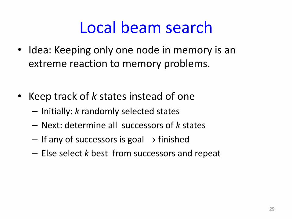
Local beam search• Idea: Keeping only one node in memory is an

extreme reaction to memory problems.

• Keep track of k states instead of one

– Initially: k randomly selected states

– Next: determine all successors of k states

– If any of successors is goal finished

– Else select k best from successors and repeat

29

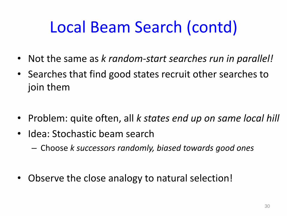
Local Beam Search (contd)

• Not the same as k random-start searches run in parallel!

• Searches that find good states recruit other searches to join them

• Problem: quite often, all k states end up on same local hill

• Idea: Stochastic beam search

– Choose k successors randomly, biased towards good ones

• Observe the close analogy to natural selection!

30

Hey! Perhaps sex can improve

search?

31

Sure! Check out ye book.

32

Genetic algorithms• Twist on Local Search: successor is generated by combining two parent states

• A state is represented as a string over a finite alphabet (e.g. binary)– 8-queens

• State = position of 8 queens each in a column

• Start with k randomly generated states (population)

• Evaluation function (fitness function): – Higher values for better states.– Opposite to heuristic function, e.g., # non-attacking pairs in 8-queens

• Produce the next generation of states by “simulated evolution”– Random selection– Crossover– Random mutation

33

8

7

6

5

4

3

2

1

String representation

16257483

Can we evolve 8-queens through genetic algorithms?

34

Evolving 8-queens

?

Sorry! Wrong queens

35

Genetic algorithms

• Fitness function: number of non-attacking pairs of queens (min = 0, max = 8 × 7/2 = 28)

• 24/(24+23+20+11) = 31%

• 23/(24+23+20+11) = 29% etc

4 states for8-queens problem

2 pairs of 2 states randomly selected based on fitness. Random crossover points selected

New statesafter crossover

Randommutationapplied

36

Genetic algorithms

Has the effect of “jumping” to a completely different newpart of the search space (quite non-local)

37

Comments on Genetic Algorithms• Genetic algorithm is a variant of “stochastic beam search”

• Positive points– Random exploration can find solutions that local search can’t

• (via crossover primarily)

– Appealing connection to human evolution

• “neural” networks, and “genetic” algorithms are metaphors!

• Negative points– Large number of “tunable” parameters

• Difficult to replicate performance from one problem to another

– Lack of good empirical studies comparing to simpler methods

– Useful on some (small?) set of problems but no convincing evidence that GAs are better than hill-climbing w/random restarts in general

• Question– are GAs really optimizing the individual fitness function? Mixability?

41

Optimization of Continuous Functions

• Discretization

– use hill-climbing

• Gradient descent

– make a move in the direction of the gradient

• gradients: closed form or empirical

42

43

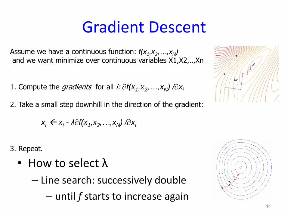
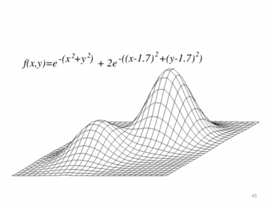
Gradient DescentAssume we have a continuous function: f(x1,x2,…,xN)

and we want minimize over continuous variables X1,X2,..,Xn

1. Compute the gradients for all i: f(x1,x2,…,xN) /xi

2. Take a small step downhill in the direction of the gradient:

xi xi - λf(x1,x2,…,xN) /xi

3. Repeat.

• How to select λ

– Line search: successively double

– until f starts to increase again44