LOCAL RISK-MINIMIZATION UNDER A PARTIALLY - DUO

Dept. of Math./CMA University ofOsloPure Mathematics No 5ISSN 0806–2439 March 2011

LOCAL RISK-MINIMIZATION UNDER A PARTIALLY OBSERVED1

MARKOV-MODULATED EXPONENTIAL LEVY MODEL2

OLIVIER MENOUKEU-PAMEN AND ROMUALD MOMEYA3

Abstract. In this paper, the option hedging problem for a Markov-modulated exponentialLevy model is examined. We employ the local risk-minimization approach to study optimalhedging strategies for Europeans derivatives under both full information and then partialinformation.

1. Introduction4

Unpredictable structural changes in the trend of asset prices or stock indexes on financial5

markets is a current reality nowadays. They are not usually caused by internal events of the6

market itself but are more related to the global socioeconomic and political environment. To7

account for these features, Markov-modulated (or regime-switching) models have since been8

widely used in econometrics and financial mathematics. See for instance, Hamilton [24] for9

exhibiting the non-stationarity of macroeconomic times series, Elliott and Van der Hoek [14]10

for asset allocation, Pliska [29] and Elliott et al. [10] for short rate models, Naik [26], Guo11

[23] and Buffington and Elliott [2] for option valuation.12

The Markov-modulated exponential Levy model is very attractive as alternative to the13

classical Black-Scholes model because they couple the benefit of an exponential Levy model14

(notably the presence of jumps) with the possibility, thanks to the Markov chain, to having15

long-term variability of some characteristics of the return distribution. However, in the con-16

text of derivative pricing these models lead to incomplete markets. Therefore, the question17

of hedging becomes a crucial one.18

In this paper, we consider the problem of optimal quadratic hedging of an European de-19

rivative contract in a market driven by a Markov-modulated Levy model. Typically, in this20

model the full information on the modulating factor X is not available in the market and the21

agent has only access to the information contained in past asset prices. Consequently, we will22

deal with an optimal quadratic hedging problem for a partially observed model (or partial23

information scenario).24

This kind of problem has been extensively studied in the literature. Di Masi, Platen25

and Runggaldier [7] were the first to discuss the problem of risk-minimizing (mean-variance)26

hedging under restricted information when the stock price is a martingale and the prices are27

observed only at discrete time instants. In [33], Schweizer explicited for general filtrations28

Date: First Version: July, 2010. This Version: April 6, 2011.2010 Mathematics Subject Classification. 60G51, 60H05, 91G10.Key words and phrases. Local risk-minimization, partial information, Levy process, regime-switching,

hedging strategy.Corresponding author: [email protected]; Phone: 0015145446440 .

1

2 OLIVIER MENOUKEU-PAMEN AND ROMUALD MOMEYA

G := Gtt∈[0,T ] ⊆ Ftt∈[0,T ] := F a risk-miminizing strategy based on G-predictable pro-29

jections. Pham [28] solved the problem of mean-variance hedging for partially observed drift30

processes. Frey and Runggaldier [17] determined a locally risk-minimizing hedging strategy31

when the asset price process follows a stochastic model and is observed only at discrete ran-32

dom times. Frey [18] considered risk-minimization with incomplete information in a model33

for high-frequency data. In the same framework but for more general model, Ceci [3] com-34

puted the optimal hedge strategy under the criterion of risk-minimization. In all these papers,35

the methodology consists first, to determine the optimal strategy under the full information36

and second, determine the final solution by projecting on the filtration available in to the37

investor. Then a natural question arises that given a Markov-modulated Levy model, can we38

applied the above methodology to study the problem of local risk-minimization under partial39

information?40

The aim of this paper is to give an answer to the previous question. In fact, we show that41

under some restrictive conditions on our Levy model, we can apply the same technics used42

by the precedent authors to obtain an optimal hedging strategy for local risk-minimization43

under partial information. In fact, we first derive a martingale representation for the wealth44

process under full information. Then we proceed as in the classical setting by solving a local45

risk minimization under full information. Let us mention that the optimal strategy obtained46

under full information is quit explicit. Finally, using the fact that our processes do not jumps47

simultaneously, we can deduce an orthogonal projection of the claim with respect to smaller48

filtration and therefore the optimal strategy.49

The paper is organized as follows. Section 2 describe in details our model setup and build50

two different filtrations that characterized the situation where investor have full or partial51

information. In Section 3, we recall some basic notions and results on risk-minimization.52

Section 4 contains the main results, namely the martingale representation property for the53

value process and the existence of optimal strategies in our market model under full and54

partial information.55

2. The model56

2.1. Framework.57

58

We consider a financial market with two primary securities, namely a money market account59

B and a stock S which are traded continuously over the time horizon T := [0, T ], where60

T ∈ (0,∞), is fixed and represents the maturity time for all economic activities. To formalize61

this market, we fix a (complete) filtered probability space (Ω,F ,F = (Ft)t∈T ,P) satisfying62

the usual conditions. We suppose also that FT = F and that F0 contains only the null sets of63

F and their complements. All processes are defined on the stochastic basis above. Further,64

we will add to this setup a filtration which specifies the flow of informations available for the65

investors.66

Let X := Xt : t ∈ T an irreducible homogeneous continuous-time Markov chain with a67

finite state space S = e1, e2, . . . , eM ⊂ RM characterized by a rate (or intensity) matrix68

A := aij : 1 ≤ i, j ≤ M. Following Dufour and Elliott [8], we can identify S with the basis69

set of the linear space RM . From now, we set ei = (0, 0, . . . , 1︸︷︷︸i−th

, . . . , 0). It follows from70

LOCAL RISK-MINIMIZATION UNDER A PARTIALLY OBSERVED MARKOV-MODULATED EXPONENTIAL LEVY MODEL3

Elliott [11] that X admits the following semimartingale representation71

Xt = X0 +

∫ t

0AXs + Γt, (2.1)

where Γ := (Γit)Mi=1 : t ∈ [0, T ] is a vector-martingale in RM with respect to the filtration72

generated by X.73

Let rt denote the instantaneous interest rate of the money market account B at time t. If74

we suppose that rt := r(t,Xt) = 〈r|Xt〉, where 〈·|·〉 is the usual scalar product in RM and75

r = (r1, r2, . . . , rM ) ∈ R+M , then the price dynamics of B is given by:76

dBt = rtBt dt, B(0) = 1 for t ∈ T . (2.2)

The appreciation rate µt and the volatility σt of the stock S at time time tare defined by77

µt := µ(t,Xt) = 〈µ|Xt〉,σt := σ(t,Xt) = 〈σ|Xt〉, t ∈ T (2.3)

where µ = (µ1, µ2, . . . , µM ) ∈ RM and σ = (σ1, σ2, . . . , σM ) ∈ R+M .78

The stock price process S is described by this following Markov modulated Levy process:79

dSt = St−(µtdt+ σtdWt +

∫R\0

(ez − 1)NX(dt; dz)), S(0) = S0 > 0 (2.4)

Here W := (Wt)t∈T is a one-dimensional standard Brownian motion or Wiener process on80

(Ω,F ,P), independent of X and NX ,81

NX(dt, dz) :=

NX(dt, dz)− ρX(dz)dt if |z| < 1NX(dt, dz) if |z| ≥ 1,

(2.5)

withNX(dt, dz) is the differential form of a Markov-modulated random measure on T ×R\0.82

We recall from Elliott and Osakwe [12] and Elliott and Royal [13] that a Markov-modulated83

random measure on T ×R\0 is a family NX(dt, dz;ω) : ω ∈ Ω of non-negative measures84

on the measurable space (T ×R\0,B(T )⊗B(R\0)), which satisfiesNX(0,R\0;ω) = 085

and has the following compensator, or dual predictable projection86

ρX(dz)dt :=

M∑i=1

〈Xt− |ei〉ρi(dz)dt, (2.6)

where ρi(dz) is the density for the jump size when the Markov chain X is in state ei and87

satisfying88 ∫|z|≥1

(ez − 1)2ρi(dz) <∞. (2.7)

The general setting considered here can be seen as an extension of the exponential-Levy model89

described in Cont and Tankov [6] where a factor of modulation is introduced. Hence, we can90

retrieve in a simple way most of some current models which exist in the literature as for91

example the classical Black-Scholes model and the family of exponential-Levy models.92

The subsequent assumption will be fundamental for obtaining our results, particularly in93

Section 4.1 to obtain a martingale representation for the value process.94

Assumption 2.1. We assume that a transition of Markov chain X from state ej to state ek95

and a jump of S do not happen simultaneously almost surely.96


Let ξ := ξtt∈T denoting the discounted stock price. Then,97

ξt :=StBt

= e−∫ t0 ruduSt.

If Rt = e∫ t0 rudu, for each t ∈ T . Then, the discounted stock price process is given by :98

dξt = Fµ(t, ξt− , Xt)dt+ Fσ(t, ξt− , Xt)dWt +

∫R\0

Fγ(t, ξt− , Xt)NX(dt; dz),

ξ(0) = S0 > 0 P a.s, (2.8)

or the following integral decomposition99

ξt = S0 +

∫ t

0Fµ(s, ξs− , Xs)ds︸︷︷︸

finite variation part

+

∫ t

0Fσ(s, ξs− , Xs)dWs +

∫ t

0

∫R\0

Fγ(s, ξs− , Xs)NX(ds; dz)︸︷︷︸

local-martingale part

,

(2.9)

where100 Fµ(t, ξt, Xt) :=

(µ(t, Rtξt, Xt)− r(t, Rtξt, Xt)

)ξt

Fσ(t, ξt, Xt) := σ(t, Rtξt, Xt)ξtFγ(t, ξt, Xt) := ξt(e

z − 1),

(2.10)

The theory of stochastic flows will also be used to identify the integrands in the stochastic101

integrals involved in the martingale representation property in Section 4.1. Let now consider102

a general form of stochastic differential equation (SDE) (2.8):103 dξt = Fµ(t, ξt− , Xt)dt+ Fσ(t, ξt− , Xt)dWt +

∫R\0 Fγ(t, ξt− , Xt)N

X(dt; dz),

ξs = x > 0 P a.s. for 0 ≤ s < t ≤ T.(2.11)

We assume that the coefficients Fµ, Fσ, Fγ are smooth enough to guaranty the existence104

and uniqueness of a strong adapted cadlag solution ξs, t(x) (see Fujiwara and Kunita [21]).105

Furthermore, this solution forms a stochastic flow of diffeomorphisms Φs, t : (0,+∞)× Ω →106

(0,+∞) given by107

Φs, t(x, ω) = ξs, t(x)(ω), (2.12)

for each (s, t) such that 0 ≤ s < t ≤ T , x ∈ (0,+∞) and ω ∈ Ω. (Φs, t)s<t verifies the108

following properties:109

• Φs, t = Φ0, t Φ−10, s for all s < t;110

• Cocycle property : Φs, u = Φt, u Φs, t for all s < t < u;111

• Conditional independent increments: for t0 ≤ t1 ≤ . . . ≤ tn,112

Φt0, t1 ,Φt1, t2 , . . . ,Φtn−1, tn are conditionally independent given FXT .113

Let x = ξ0, t(x0), for each t ∈ [0, T ]. By the uniqueness of solutions of SDE and the semi-group114

property, we get115

ξ0, T (x0) = ξt, T (ξ0, t(x0)) = ξt, T (x). (2.13)

Differentiating (2.13) with respect to x0, we obtain:116

∂ξ0,T (x0)

∂x0=∂ξt, T (x)

∂x

∂ξ0, t(x0)

∂x0. (2.14)


2.2. Market information.117

118

In general, the Markov-modulated Levy model as described by Equation (2.4) is based on119

the mathematical framework of the Markov additive processes (MAP). This last object is120

an old and widely studied subject in stochastic analysis (see, e.g, [4, 5, 16, 22] for a few.)121

In particular, the couple (X,S) is a Markov additive process and yields to two important122

filtrations as we will see below.123

Let FX := FXt t∈T and FS := FSt t∈T denote the right-continuous, P−complete filtra-124

tions generated by X et S respectively. We define for t ∈ T ,125

Gt := FSt (2.15)

and126

Gt := FXT ∨ FSt . (2.16)

The filtration G := Gtt∈T represents all the information up to time t gained from the127

observations of the price fluctuations S. The strict larger filtration G := Gtt∈T denotes the128

information about the stock price history up to time t and the information about the entire129

path FXT of the modulation factor process X.130

We will assume in the last section of is paper that the investors in the market only have131

access to the first filtration which is thus the one used practically whereas the last serves132

mainly theoretical purposes.133

2.3. Esscher transform change of measure.134

135

One of the main features of the Markov-modulated Levy model is that it leads to an136

incomplete market. We shall therefore employ the regime-switching Esscher transform as in137

Elliott et al. [11] to determine an equivalent martingale measure.138

For doing so, we define the process Y by139

Yt =

∫ t

0

(µr −

1

2σ2r

)dr +

∫ t

0σrdWr +

∫ t

0

∫R\0

zNX(dr; dz)−∫ t

0

∫R\0

(ez − 1− z)ρX(dz)dr

(2.17)

As in [35], let consider the following set140

Θ :=

(θt)t∈T | θt :=

N∑i=1

θi〈Xt− |ei〉 with (θ1, θ2, ..., θN ) ∈ RN such that EP[e−

∫ t0 θrdYr

∣∣∣FXT ] <∞.

For θ := (θt)t∈T ∈ Θ, the generalized Laplace transform of a G-adapted process Y is defined141

as142

MY (θ)t := EP[e−

∫ t0 θrdYr

∣∣∣FXT ]. (2.18)

Notice that contrary to the usual Esscher transform, the expectation involved here is taken143

conditionally on the information of all the future of the Markov chain X. With this extended144

definition of a Laplace transform, we can now define the generalized Esscher transform (with145

respect to the parameter θ called Esscher parameter).146


Let Λθ = Λθtt∈T denote a G-adapted stochastic process defined as147

Λθt :=e−

∫ t0 θrdYr

MY (θ)t, t ∈ T ; θ ∈ Θ. (2.19)

It can be shown that (see for example, [11])148

Λθt = exp

[−∫ t

0θrσrdWr −

1

2

∫ t

0θ2rσ

2rdr −

∫ t

0

∫R\0

θr−zNX(dr; dz)

−∫ t

0

∫R\0

(e−zθr − 1 + θrz

)ρX(dz)dr

]. (2.20)

Moreover, as proven in [35], the stochastic process Λθ = Λθtt∈T defined by (2.19) is a positive149

(G,P)-martingale and150

EP[Λθt ] = 1, ∀t ∈ T . (2.21)

From Equation 2.21, we deduce that the process Λθ = Λθtt∈T given by Equation (2.20) is151

a density process inducing a change of measure in the probability space (Ω,GT ). Indeed, by152

setting153

dQθ

dP

∣∣∣Gt

= Λθt t ∈ T , (2.22)

we define for each process θ in Θ a new probability measure Qθ equivalent to P. Actually, Qθ154

is just an equivalent probability measure, to transform it into a martingale equivalent measure155

we need to impose some conditions generally known as martingale condition. It stipulates156

that the discounted stock price ξtt∈T would be a G-martingale under Qθ. Then,157

EQθ[ξt|G0

]= ξ(0), ∀t ∈ T . (2.23)

Hence, we have158

Proposition 2.2. An equivalent probability measure Qθ defined through (2.22) is an equiva-159

lent martingale measure on (Ω,GT ), i.e. it satisfies condition (2.23), if and only if the process160

θ satisfies the following equation161

µt − rt − θtσ2t +

∫R\0

(ez − 1)(e−zθt − 1)ρX(dz) = 0, ∀t ∈ T . (2.24)

Proof. The proof is a straightforward adaptation of that of Proposition 2.2 in Elliott et al.162

[11]. The main ingredient is an explicit computation of the generalized Laplace transform163

defined by (2.18). 164

However, the process θ is completely determined by the vector (θ1, θ2, . . . , θM ) solution of165

the system of equations166

µi − ri − θiσ2i +

∫R

(ez − 1)(e−zθi − 1)ρi(z)dz = 0, (2.25)

for i = 1, 2, . . . , N .167

168

For pricing purposes, we need to know the dynamics of the discounted stock price under the169

martingale probability measure Qθ. The following proposition states a result in this direction.170


Proposition 2.3. Under risk-neutral probability measure Qθ, the discounted stock price pro-171

cess ξ is solution to the following stochastic differential equation172 dξt = Fσ(t, ξt− , Xt)dW

θt +

∫R\0 Fγ(t, ξt− , Xt)N

θ(dt; dz)

ξ(0) = S0 > 0 P-a.s. for 0 ≤ t ≤ T,(2.26)

where173

• W θ defined by174

W θt := Wt +

∫ t

0θrσrdr, (2.27)

is the standard Brownian motion under Qθ;175

• Nθ

defined by176

Nθ(dr; dz) = NX(dr; dz)− ρθX (dz)dr, (2.28)

is the compensated measure of NX under Qθ with ρθX

(dz) := e−θzρX(dz).177

178

Proof. This follows easily from Equation (2.8) by the application of Girsanov-Meyer Theorem179

(See Øksendal and Sulem [27], Protter [30]). 180

3. The locally risk-minimizing hedging problem181

In this section, we recall some terminology on local risk minimization. We shall simply give182

necessary results; for further informations, the reader is referred to the survey of Schweizer183

[34] from which our presentation owes much.184

3.1. Review of some notions on the risk-minimization approach.185

186

This concept has been introduced by Follmer and Sondermann [20] for nonredundant (ornon-attainable) contingent claim written on a one-dimensional, square-integrable discountedrisky asset ξ which is a martingale under the original measure P. Concretely, given a stochasticbasis as above the goal consist to minimize the conditional remaining risk : Rt := EP[(CT −Ct)

2|Ft] for all t ∈ T . Here Ct stands for the cost process and is defined as the differencebetween the value of the (portfolio) strategy detained by the investor at time t and the gainsmade from trading in the financial market up to time t. Let L2(ξ) the space of all R-valuedpredictable process φ such that

||φ||L2(ξ) :=(EP[ ∫ T

0φ2ud[ξ, ξ]u

]) 12<∞,

A trading strategy is a pair of processes ϕ = (φ, ψ) where ψ is an adapted process and187

φ ∈ L2(ξ) is a F-predictable process, such that the value process V := φξ + ψ has right188

continuous sample paths and EP[V 2t ] <∞ for every t ∈ T (i.e Vt ∈ L2(Ω,P) for every t ∈ T ).189

For a trading strategy ϕ = (φ, ψ), where φ = (φt)t∈T denotes at time t, the number of190

stocks held and ψ = (ψt)t∈T the amount invested in the money market account.191

Let H be a claim which is FT -measurable and square-integrable. Consider a strategies thatreplicate the contingent claim H at time T ; that is the strategies with the assumption

VT = H P-a.s.


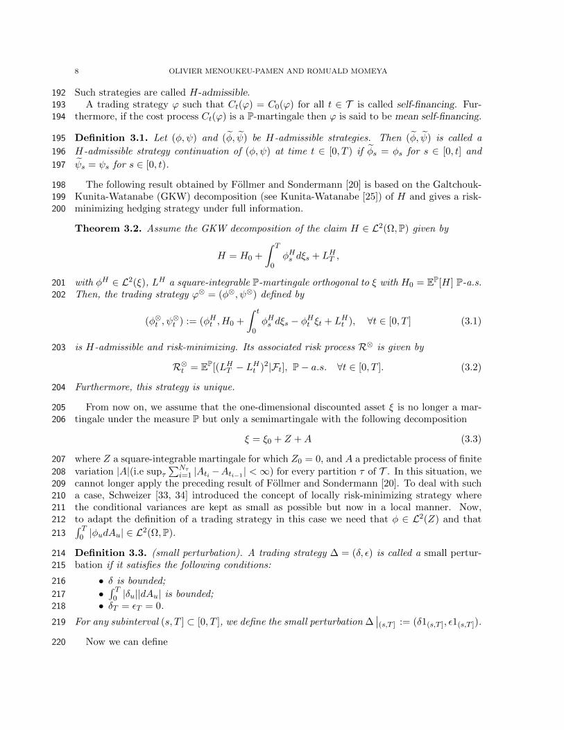
Such strategies are called H-admissible.192

A trading strategy ϕ such that Ct(ϕ) = C0(ϕ) for all t ∈ T is called self-financing. Fur-193

thermore, if the cost process Ct(ϕ) is a P-martingale then ϕ is said to be mean self-financing.194

Definition 3.1. Let (φ, ψ) and (φ, ψ) be H-admissible strategies. Then (φ, ψ) is called a195

H-admissible strategy continuation of (φ, ψ) at time t ∈ [0, T ) if φs = φs for s ∈ [0, t] and196

ψs = ψs for s ∈ [0, t).197

The following result obtained by Follmer and Sondermann [20] is based on the Galtchouk-198

Kunita-Watanabe (GKW) decomposition (see Kunita-Watanabe [25]) of H and gives a risk-199

minimizing hedging strategy under full information.200

Theorem 3.2. Assume the GKW decomposition of the claim H ∈ L2(Ω,P) given by

H = H0 +

∫ T

0φHs dξs + LHT ,

with φH ∈ L2(ξ), LH a square-integrable P-martingale orthogonal to ξ with H0 = EP[H] P-a.s.201

Then, the trading strategy ϕ⊗ = (φ⊗, ψ⊗) defined by202

(φ⊗t , ψ⊗t ) := (φHt , H0 +

∫ t

0φHs dξs − φHt ξt + LHt ), ∀t ∈ [0, T ] (3.1)

is H-admissible and risk-minimizing. Its associated risk process R⊗ is given by203

R⊗t = EP[(LHT − LHt )2|Ft], P− a.s. ∀t ∈ [0, T ]. (3.2)

Furthermore, this strategy is unique.204

From now on, we assume that the one-dimensional discounted asset ξ is no longer a mar-205

tingale under the measure P but only a semimartingale with the following decomposition206

ξ = ξ0 + Z +A (3.3)

where Z a square-integrable martingale for which Z0 = 0, and A a predictable process of finite207

variation |A|(i.e supτ∑Nτ

i=1 |Ati −Ati−1 | <∞) for every partition τ of T . In this situation, we208

cannot longer apply the preceding result of Follmer and Sondermann [20]. To deal with such209

a case, Schweizer [33, 34] introduced the concept of locally risk-minimizing strategy where210

the conditional variances are kept as small as possible but now in a local manner. Now,211

to adapt the definition of a trading strategy in this case we need that φ ∈ L2(Z) and that212 ∫ T0 |φudAu| ∈ L

2(Ω,P).213

Definition 3.3. (small perturbation). A trading strategy ∆ = (δ, ε) is called a small pertur-214

bation if it satisfies the following conditions:215

• δ is bounded;216

•∫ T

0 |δu||dAu| is bounded;217

• δT = εT = 0.218

For any subinterval (s, T ] ⊂ [0, T ], we define the small perturbation ∆∣∣(s,T ] := (δ1(s,T ], ε1(s,T ]).219

Now we can define220


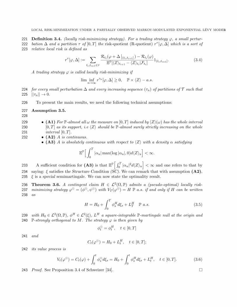
Definition 3.4. (locally risk-minimizing strategy). For a trading strategy ϕ, a small pertur-221

bation ∆ and a partition τ of [0, T ] the risk-quotient (R-quotient) rτ [ϕ,∆] which is a sort of222

relative local risk is defined as223

rτ [ϕ,∆] :=∑

ti,ti+1∈τ

Rti(ϕ+ ∆∣∣(ti,ti+1] )−Rti(ϕ)

EP[〈Z〉ti+1 − 〈Z〉ti |Fti ]1(ti,ti+1]. (3.4)

A trading strategy ϕ is called locally risk-minimizing if

lim infn→∞

rτn [ϕ,∆] ≥ 0, P× 〈Z〉 − a.s.

for every small perturbation ∆ and every increasing sequence (τn) of partitions of T such that224

||τn|| → 0.225

To present the main results, we need the following technical assumptions:226

Assumption 3.5.227

228

• (A1) For P-almost all ω the measure on [0, T ] induced by 〈Z〉(ω) has the whole interval229

[0, T ] as its support, i.e 〈Z〉 should be P-almost surely strictly increasing on the whole230

interval [0, T ].231

• (A2) A is continuous.232

• (A3) A is absolutely continuous with respect to 〈Z〉 with a density α satisfying

EP[ ∫ T

0|αu|max(log |αu|, 0)d〈Z〉u

]<∞.

A sufficient condition for (A3) is that EP[ ∫ T

0 |αu|2d〈Z〉u

]< ∞ and one refers to that by233

saying: ξ satisfies the Structure Condition (SC). We can remark that with assumption (A2),234

ξ is a special semimartingale. We can now state the optimality result.235

Theorem 3.6. A contingent claim H ∈ L2(Ω,P) admits a (pseudo-optimal) locally risk-236

minimizing strategy ϕ = (φ, ψ) with VT (ϕ) = H P a.s. if and only if H can be written237

as238

H = H0 +

∫ T

0φHs dξs + LHT P a.s. (3.5)

with H0 ∈ L2(Ω,P), φH ∈ L2(ξ), LH a square-integrable P-martingale null at the origin and239

P-strongly orthogonal to M . The strategy ϕ is then given by240

φt = φHt , t ∈ [0, T ]

and241

Ct(ϕ) = H0 + LHt , t ∈ [0, T ];

its value process is242

Vt(ϕ) = Ct(ϕ) +

∫ t

0φs dξs = H0 +

∫ t

0φHs dξs + LHt , t ∈ [0, T ]. (3.6)

Proof. See Proposition 3.4 of Schweizer [34]. 243


Equation (3.5) is called Follmer-Schweizer decomposition (FS) for the contingent claim244

H. In practice, to obtain this decomposition is very difficult so the more natural approach245

introduced by Follmer and Schweizer [19] consist to use a Girsanov transformaton to shift246

the problem back to a martingale measure where standard techniques as Galchouk-Kunita-247

Watanabe projection is available.248

4. Main results249

4.1. A martingale representation property.250

251

In this section, we give an explicit representation of a martingale which is useful for the252

problem of hedging in the context of a Markov-modulated Levy model. The proof of the result253

is similar to the one given by Elliott et al. [15]. We give an explicit martingale representation254

of the wealth process which will be useful later on in the finding of an optimal strategy the255

proof of our main result.256

First, it is easy to see that the Esscher transform change of measure Λθ introduced in257

Section 2.3 is solution to this following SDE258

Λt, u(x) = 1 +

∫ ut Λt, r−(x)(−θrσr)(r, ξt, r−(x), Xr)dWr

+∫ ut

∫R\0 Λt, r−(x)(e−zθr(r,ξt, r− (x),Xr) − 1)NX(dr; dz)

Λt, t(x) = 1 P a.s. for 0 ≤ t < u ≤ T.(4.1)

Indeed, for all t ∈ [0, T ], Λθt = Λ0, t(x).259

260

Now, consider a function c(·) : (0,+∞) → R such that c(·) is twice differentiable and c(·)261

and ∂c(·)∂x are at most linear growth in x. We shall determine the current price at time t of a262

contingent claim of the form c(ST ), which is the payoff of the claim at maturity T > t. In the263

sequel, we have to work with the discounted claim as function of the discounted stock price,264

that is:265

c(ξ0,T ) := R−1T c(RT ξ0,T (x0)) = R−1

T c(ST ). (4.2)

So, we assume that the process θ is chosen such that EQθ [c2(ξ0,T (x0))] < ∞ and then we266

define the square-integrable (G,Qθ)-martingale Vtt∈[0,T ] as:267

Vt := EQθ [c(ξ0,T (x0))|Gt], t ∈ [0, T ]. (4.3)

As (X, ξ) and (X,Λ) are Markov additive processes (See Cinlar [4]) we have that they verify268

the Markov property with respect to the large filtration G. Hence, we obtain by using269


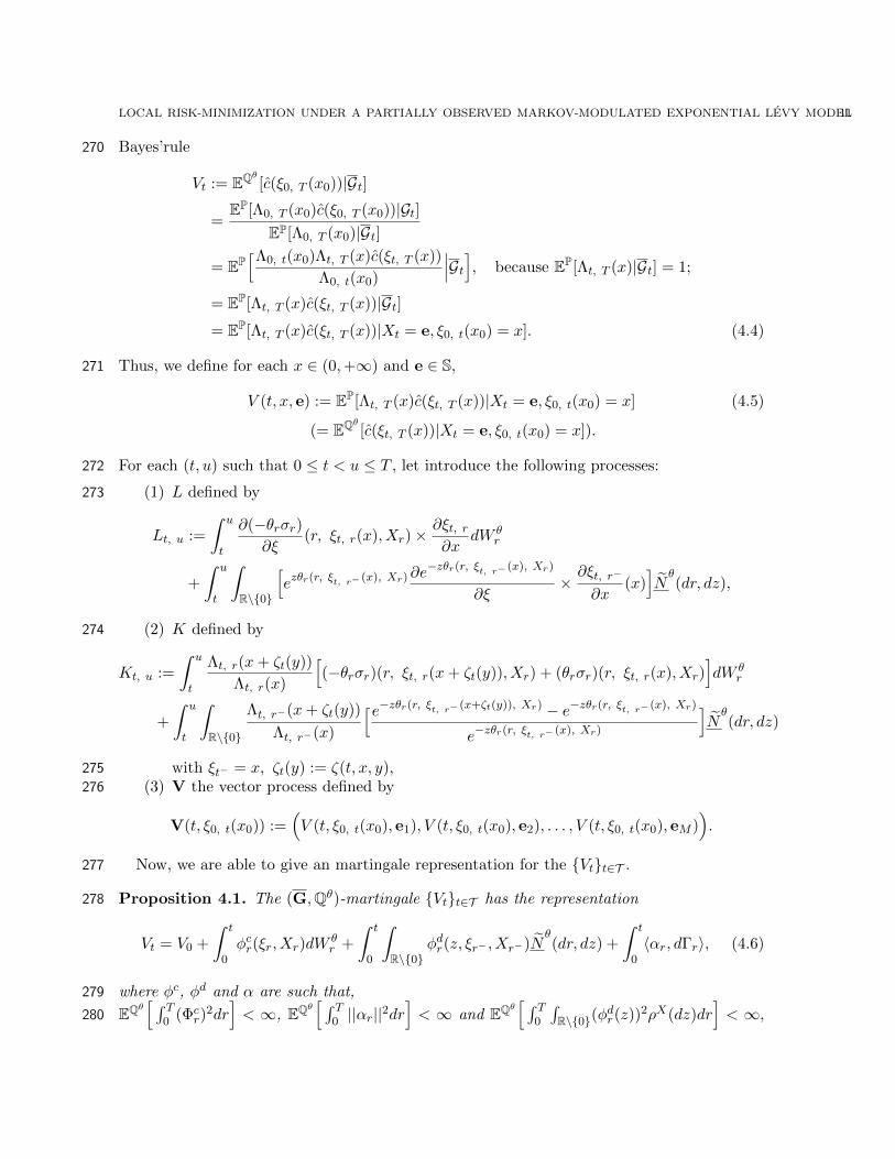
Bayes’rule270

Vt := EQθ [c(ξ0, T (x0))|Gt]

=EP[Λ0, T (x0)c(ξ0, T (x0))|Gt]

EP[Λ0, T (x0)|Gt]

= EP[Λ0, t(x0)Λt, T (x)c(ξt, T (x))

Λ0, t(x0)

∣∣∣Gt], because EP[Λt, T (x)|Gt] = 1;

= EP[Λt, T (x)c(ξt, T (x))|Gt]= EP[Λt, T (x)c(ξt, T (x))|Xt = e, ξ0, t(x0) = x]. (4.4)

Thus, we define for each x ∈ (0,+∞) and e ∈ S,271

V (t, x, e) := EP[Λt, T (x)c(ξt, T (x))|Xt = e, ξ0, t(x0) = x] (4.5)

(= EQθ [c(ξt, T (x))|Xt = e, ξ0, t(x0) = x]).

For each (t, u) such that 0 ≤ t < u ≤ T , let introduce the following processes:272

(1) L defined by273

Lt, u :=

∫ u

t

∂(−θrσr)∂ξ

(r, ξt, r(x), Xr)×∂ξt, r∂x

dW θr

+

∫ u

t

∫R\0

[ezθr(r, ξt, r− (x), Xr)∂e

−zθr(r, ξt, r− (x), Xr)

∂ξ×∂ξt, r−

∂x(x)]Nθ(dr, dz),

(2) K defined by274

Kt, u :=

∫ u

t

Λt, r(x+ ζt(y))

Λt, r(x)

[(−θrσr)(r, ξt, r(x+ ζt(y)), Xr) + (θrσr)(r, ξt, r(x), Xr)

]dW θ

r

+

∫ u

t

∫R\0

Λt, r−(x+ ζt(y))

Λt, r−(x)

[e−zθr(r, ξt, r− (x+ζt(y)), Xr) − e−zθr(r, ξt, r− (x), Xr)

e−zθr(r, ξt, r− (x), Xr)

]Nθ(dr, dz)

with ξt− = x, ζt(y) := ζ(t, x, y),275

(3) V the vector process defined by276

V(t, ξ0, t(x0)) :=(V (t, ξ0, t(x0), e1), V (t, ξ0, t(x0), e2), . . . , V (t, ξ0, t(x0), eM )

).

Now, we are able to give an martingale representation for the Vtt∈T .277

Proposition 4.1. The (G,Qθ)-martingale Vtt∈T has the representation278

Vt = V0 +

∫ t

0φcr(ξr, Xr)dW

θr +

∫ t

0

∫R\0

φdr(z, ξr− , Xr−)Nθ(dr, dz) +

∫ t

0〈αr, dΓr〉, (4.6)

where φc, φd and α are such that,279

EQθ[ ∫ T

0 (Φcr)

2dr]< ∞, EQθ

[ ∫ T0 ||αr||

2dr]< ∞ and EQθ

[ ∫ T0

∫R\0(φ

dr(z))

2ρX(dz)dr]< ∞,280


with the following explicit expressions281

φcr(ξr, Xr) = EQθ[Lr, T c(ξr, T (x)) +

∂c

∂ξ(ξr, T (x))

∂ξr, T∂x

(x)∣∣∣Xr = e, ξ0, r(x0) = x

]σr(r, ξr, Xr);

(4.7)

φdr(y, ξr− , Xr) = EQθ[(Kr, T + 1)c(ξr, T (x− + ζr(z)))− c(ξr, T (x))

∣∣∣Xr = e, ξ0, r(x0) = x];

(4.8)

αt = V(t, ξ0, t(x0)) ∈ RM . (4.9)

with x = ξ0, r(x0) and x− = ξ0, r−(x0).282

In order to prove Proposition 4.1, we need the subsequent result283

Lemma 4.2. The following identities hold284

∂Λt, T∂x

(x) = Λt, T (x)× Lt, T (4.10)

and285

Λt, T (x+ ζ(z))− Λ(x) = Λt, T (x)×Kt, T . (4.11)

Proof. See Appendix. 286

Now, we give the proof of the Proposition 4.1.287

Proof. (Proposition 4.1)288

289

Noting that290

V (t, ξt, Xt) = 〈V(t, ξt)|Xt〉, (4.12)

we obtain dy differentiation291

dV (t, ξt, Xt) = 〈dV(t, ξt)|Xt〉+ 〈V(t, ξt)|dXt〉, (4.13)

and from Ito differentiation rule292

dV (t, ξt, Xt) =

⟨V(t, ξt)

∣∣∣∣∣dXt

⟩+

⟨∂V

∂tdt+

∂V

∂ξdξt +

1

2

∂2V

∂ξ2d[ξ, ξ]ct (4.14)

+

∫R\0

[V(t, ξt−e

z)−V(t, ξt−)−∆ξt∂V

∂ξ

]NX(dt, dz)

∣∣∣∣∣Xt

⟩From (3.3), we deduce that293

dXt = AXt−dt+ dΓt. (4.15)


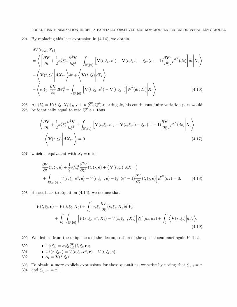
By replacing this last expression in (4.14), we obtain294

dV (t, ξt, Xt)

=

⟨[∂V

∂t+

1

2σ2t ξ

2t−∂2V

∂ξ2+

∫R\0

[V(t, ξt−e

z)−V(t, ξt−)− ξt−(ez − 1)∂V

∂ξ

]ρθ

X(dz)

]dt

∣∣∣∣∣Xt

⟩

+

⟨V(t, ξt)

∣∣∣∣∣AXt−

⟩dt+

⟨V(t, ξt)

∣∣∣∣∣dΓt

⟩

+

⟨σtξt−

∂V

∂ξdW θ

t +

∫R\0

[V(t, ξt−e

z)−V(t, ξt−)]Nθ(dt, dz)

∣∣∣∣∣Xt

⟩(4.16)

As Vt = V (t, ξt, Xt)t∈T is a (G,Qθ)-martingale, his continuous finite variation part would295

be identically equal to zero Qθ a.s, thus296 ⟨∂V

∂t+

1

2σ2t ξ

2t

∂2V

∂ξ2+

∫R\0

[V(t, ξt−e

z)−V(t, ξt−)− ξt−(ez − 1)∂V

∂ξ

]ρθ

X(dz)

∣∣∣∣∣Xt

⟩

+

⟨V(t, ξt)

∣∣∣∣∣AXt−

⟩= 0 (4.17)

which is equivalent with Xt = e to:297

∂V

∂t(t, ξt, e) +

1

2σ2t ξ

2t

∂2V

∂ξ2(t, ξt, e) +

⟨V(t, ξt)

∣∣∣AXt−

⟩+

∫R\0

[V (t, ξt−e

z, e)− V (t, ξt− , e)− ξt−(ez − 1)∂V

∂ξ(t, ξt, e)

]ρθ

X(dz) = 0. (4.18)

Hence, back to Equation (4.16), we deduce that298

V (t, ξt, e) = V (0, ξ0, X0) +

∫ t

0σsξs

∂V

∂ξ(s, ξs, Xs)dW

θs

+

∫ t

0

∫R\0

[V (s, ξs−e

z, Xs)− V (s, ξs− , Xs)]Nθ(ds, dz) +

∫ t

0

⟨V(s, ξs)

∣∣∣dΓs

⟩.

(4.19)

We deduce from the uniqueness of the decomposition of the special semimartingale V that299

• Φct(ξt) = σtξt

∂V∂ξ (t, ξt, e);300

• Φdt (z, ξt−) = V (t, ξt−e

z, e)− V (t, ξt, e);301

• αt = V(t, ξt).302

To obtain a more explicit expressions for these quantities, we write by noting that ξ0, t = x303

and ξ0, t− = x−304


Φct(ξt) = xσt(t, x, e)

∂V

∂x(t, x, e)

= xσt(t, x, e)∂

∂xEP[Λt, T (x)c(ξt, T (x))|Xt = e, ξ0, t(x0) = x] by (4.5)

= xσt(t, x, e)EP[∂Λt, T

∂x(x)c(ξt, T (x)) + Λt, T (x)

∂c

∂ξ(ξt, T (x))

∂ξt, T∂x

(x)∣∣∣Xt = e, ξ0, t(x0) = x

]= xσt(t, x, e)EP

[Λt, T (x)Lt, T c(ξt, T (x))

+ Λt, T (x)∂c

∂ξ(ξt, T (x))

∂ξt, T∂x

(x)∣∣∣Xt = e, ξ0, t(x0) = x

]by Lemma 4.2

= xσt(t, x, e)EQθ[Lt, T c(ξt, T (x)) +

∂c

∂ξ(ξt, T (x))

∂ξt, T∂x

(x)∣∣∣Xt = e, ξ0, t(x0) = x

]. (4.20)

In the same way,305

Φdt (z, ξt−) = V (t, ξt−e

z, e)− V (t, ξt− , e)

= EP[Λt, T (x− + ζr(z))c(ξt, T (x− + ζr(z)))

∣∣∣Xt = e, ξ0, t(x0) = x]

− EP[Λt, T (x)c(ξt, T (x))

∣∣∣Xt = e, ξ0, t(x0) = x]

= EP[(

Λt, T (x− + ζr(z))− Λt, T (x))c(ξt, T (x− + ζr(z)))

∣∣∣Xt = e, ξ0, t(x0) = x]

+ EP[Λt, T (x)

(c(ξt, T (x− + ζr(z)))− c(ξt, T (x))

)∣∣Xt = e, ξ0, t(x0) = x]

= EP[Λt, T (x)Kt,T

(c(ξt, T (x− + ζr(z))

)+ Λt, T (x)

(c(ξt, T (x− + ζr(z)))− c(ξt, T (x))

)∣∣∣Xt = e, ξ0, t(x0) = x]

by Lemma 4.2

= EQθ[(Kt,T + 1)c(ξt, T (x− + ζr(z)))− c(ξt, T (x))

∣∣∣Xt = e, ξ0, t(x0) = x]. (4.21)

Finally, we have to show that the different component involved in (4.19) are mutually or-306

thogonal (G,Qθ)-local martingale, that is, the different product W θ · N θ(·, dz), W θ · Γ and307

Γ·N θ(·, dz) are (G,Qθ)-local martingale. The claim is easy verified for the first ones by noting308

that W θ is an continuous (G,Qθ) local-martingale such that W θ0 = 0 whereas N

θ(·, dz) and Γ309

are pure jump (G,Qθ) local-martingales. For the last, we have ∀t ∈ T and ∀i ∈ 1, 2, ...,M310

[Γi, Nθ(·, dz)]t =

∑0≤s≤t

∆Γis∆Nθ(s, dz)

= 0. (4.22)

This result comes from Assumption 2.1 and the decomposition theorem of the (additive)311

component of the MAP (X,S) given in Cinlar [5], theorem 2.23. 312

4.2. The locally risk-minimizing hedging Problem under full information for the313

model (2.4)-(2.2).314

315


In this section, we consider the problem of hedging a contingent claim H in the Markov-316

modulated exponential Levy model given by (2.2)-(2.4) given that the information set is G.317

In general, in such a market the claim H cannot be perfectly hedged. Therefore, we need318

to take into account the market participant’s attitude toward risk in the search of the viable319

market transactions. One way of doing this in the literature consists to optimize a given320

criterion based or not on the preference of the market participant. In particular, the choice321

of quadratic criterion is quite natural and pertinent because it leads to a linear pricing rule322

which is very meaningful in financial economics.323

Let B be a contingent claim with a discounted payoff H = c(ξ0, T (x0)) ∈ L2(Ω,P). Follow-324

ing Schweizer [32], a locally risk-minimizing strategy ϕ = (φ, ψ) which generates c(ξ0, T (x0))325

must be such that326

(1) VT = c(ξ0, T (x0)) P-a.s.;327

(2) Vt(ϕ) = V0(ϕ) +∫ t

0 φrdξr + Υt, for all t ∈ [0, T ];328

(3) Υ is a martingale under P and Υ is orthogonal to the martingale part Z of ξ under P.329

We shall require that (Vt(ϕ))0≤t≤T is a (G,Qθ)-martingale. With this assumption and Equa-330

tion (4.5), we have331

Vt(ϕ) = EQθ [VT (ϕ)|Gt]= EQθ [c(ξ0, T (x0))|Xt = e, ξ0, t = x]

= V (t, x, e).

Now we can state the main proposition if this section.332

Proposition 4.3. Assume σt > 0 for all t ∈ [0, T ]. If there exists a process θ∗ satisfying333

(2.24) and such that334

θ∗t =µt − rt

σ2t +

∫R\0(e

x − 1)2ρX(dx), (4.23)

335

e−zθ∗t − 1 = − (µt − rt)(ez − 1)

σ2t +

∫R\0(e

x − 1)2ρX(dx), ∀z ∈ R (4.24)

then there exists a minimal martingale measure defined by the Esscher transform Λθ∗. Fur-336

thermore, the locally risk-minimizing strategy for the contingent claim H is given by337

φ∗t =1

ξt−×σtφ

ct(ξt, Xt) +

∫R\0(e

z − 1)φdt (y, ξt− , Xt−)ρX(dz)

σ2t +

∫R\0(e

x − 1)2ρX(dx), (4.25)

and338

ψ∗t := Vt(ϕ)− φ∗t ξt= EQθ∗ [c(ξ0, T (x0))|Xt = e, ξ0, t = x]− φ∗t ξt. (4.26)

Proof.339

1- We have to show that if there exists a process θ∗ satisfies the Equations (2.24), (4.23) and340

(4.24) then the process Λθ∗

defines a minimal martingale measure in the sense of Schweizer341

[31].342


Indeed, under these assumptions we have from Equation (4.1)343

Λθ∗t = 1 +

∫ t

0Λθ∗

s−(−θ∗sσs)dWs +

∫ t

0

∫R\0

(ez − 1)NX(ds, dz)

= 1−∫ t

0Λθ∗

s−

[ µs − rsσ2s +

∫R\0(e

x − 1)2ρX(dx)

][σsdWs +

∫R\0

(ez − 1)NX(ds, dz)]

= 1−∫ t

0Λθ∗

s−1

ξs−×[ µs − rsσ2s +

∫R\0(e

x − 1)2ρX(dx)

]dZs, (4.27)

where Z denoted the martingale part of the (special) semimartingale ξ. Using Assumptions344

4.23 and 4.24, it is easy to see that the process λ given for t ∈ T by:345

λt :=dAtd〈Z〉t

=1

ξt−×σ2t θ∗t +

∫R\0(e

z − 1)(e−θ∗t z − 1)ρX(dz)

σ2s +

∫R\0(e

x − 1)2ρX(dx)

=1

ξt−× µt − rtσ2t +

∫R\0(e

x − 1)2ρX(dx)(4.28)

is G-predictable and verifies∫ t

0 λ2sd〈Z〉s <∞ P-a.s. Hence, we see that346

Λθ∗t = 1−

∫ t

0Λθ∗

s−λsdZs. (4.29)

This defines precisely the minimal martingale measure according Follmer and Schweizer [19].347

In the sequel we will denote it by Qθ∗ .348

2- From Follmer and Schweizer ([19]) we now that once a MMM is found, the locally349

risk-minimizing strategy of the contingent claim is uniquely determined from the (G,Qθ∗)-350

projection of Galtchouk-Kunita-Watanabe decomposition of c(ξ0, T (x0)). From Proposition351

4.1, we have for all t ∈ [0, T ],352

Vt = V0 +

∫ t

0φcr(ξr, Xr)dW

θ∗r +

∫ t

0

∫R\0

φdr(z, ξr− , Xr−)Nθ∗

(dr, dz) +

∫ t

0〈αr|dΓr〉 (4.30)

where φc and φd are given by Equations (4.7) and (4.8) respectively. Therefore, we have from353

(2)354

Υt = Vt(ϕ)−∫ t

0φrdξr − V0(ϕ)

=

∫ t

0

[φcr(ξr, Xr)− σrξrφr

][dWr + θ∗t σrdr

]+

∫ t

0

∫R\0

[φdr(z, ξr− , Xr−)− ξr−(ez − 1)φr

][NX(dr, dz)− ρX(dz)dr − (e−θ

∗rz − 1)ρX(dz)dr

]+

∫ t

0〈αr|dΓr〉. (4.31)


From (3), Υ should be a (G,P)-martingale thus the drift term in (4.31) should be zero or355

equivalently356

ξt−φt

[ ∫R\0

(ez − 1)(e−θ∗t z − 1)ρX(dz)− θ∗t σ2

t

]=

∫R\0

φdt (z, ξt− , Xt−)(e−θ∗t z − 1)ρX(dz)− φct(ξt, Xt)θ

∗t σt. (4.32)

Hence357

Υt =

∫ t

0[φcr(ξr, Xr)− σrξrφr]dWr +

∫ t

0〈αr|dΓr〉

+

∫ t

0

∫R\0

[φdr(z, ξr− , Xr−)− ξr−(ez − 1)φr]NX(dr, dz). (4.33)

The requirement (3) stipulates also that Υ is orthogonal to the martingale part Z of ξ under358

P. This is verified if and only if ΥZ is a (G,P)-martingale, therefore359

ξt−φt

[ ∫R\0

(ex − 1)2ρX(dx) + σ2t

]= φct(ξt, Xt)σt +

∫R\0

φdt (z, ξr− , Xr−)(ez − 1)ρX(dz).

(4.34)360

Recalling the martingale condition (2.24) and substituting it in Equation (4.32) we obtain361

ξt−φt(rt − µt) =

∫R\0

φdt (z, ξt− , Xt−)(e−θ∗t z − 1)ρX(dz)− φct(ξt, Xt)θ

∗t σt, (4.35)

and using Equation (4.34), we get that θ∗ satisfies362 [θ∗t −

µt − rtσ2t +

∫R\0(e

x − 1)2ρX(dx)

]φct(ξt, Xt)σt

−∫R\0

[(e−θ

∗t z − 1) +

(µt − rt)(ez − 1)

σ2t +

∫R\0(e

x − 1)2ρX(dx)

]φdt (y, ξt− , Xt−)ρX(dz) = 0. (4.36)

Thus, if there exists a process θ∗ verifying (2.24) and such that ∀t ∈ [0, T ]363

θ∗t =µt − rt

σ2t +

∫R\0(e

x − 1)2ρX(dx)

and364

e−θ∗t z − 1 = − (µt − rt)(ez − 1)

σ2t +

∫R\0(e

x − 1)2ρX(dx), ∀z ∈ R\0.

Then a locally risk-minimizing strategy exists (independently of the claim to be hedged) and365

is deduced from Equations (4.34) and (3.1)366 φ∗t = 1ξt−×

σtφct+∫R\0 φ

dt−

(z)(ez−1)ρX(dz)

σ2t+

∫R\0(e

x−1)2ρX(dx)

ψ∗t = V0 +∫ t

0 φ∗sdξs − φ∗t ξt + Γt.

(4.37)

The expression of ψ∗ follows from the definition of the portfolio value process V and this ends367

the proof . 368


We can derive easily the expression of the residual G-risk process Υ for all t ∈ T as369

Υt =

∫ t

0

1

σ2r +

∫R\0(e

x − 1)2ρX(dx)×[φcr

∫R\0

(ez−1)2ρX(dz)−σr∫R\0

φdr−(z)(ez−1)ρX(dz)]dWr

+

∫ t

0

∫R\0

1

σ2r +

∫R\0(e

x − 1)2ρX(dx)×[σ2rφ

dr−(z)−(ez−1)σrφ

cr

]NX(dr, dz)+

∫ t

0〈αr|dΓr〉.

(4.38)

Remark 4.4. It is possible that Equation 4.36 has not a unique solution, for example if370

φc ≡ 0 ≡ φd.371

4.3. The locally risk-minimizing hedging Problem under partial information.372

373

This section considers the problem of the local risk-minimization of the contingent claim374

H when the asset dynamics follows Equation (2.4) from the viewpoint of an investor/hedger375

which does not have at his disposal the full information as described by the filtration G =376

Gtt∈T but only the information set G = Gtt∈T ; with Gt ⊂ Gt for all t ∈ T . We have377

that GT = GT thus the contingent claim H = c(ξ0,T (x0)) which is GT -measurable will also378

GT -measurable.379

We aim at finding a G-locally risk-minimizing strategy. From the previous section, we have380

the following representation381

Vt(ϕ∗) = V0(ϕ∗) +

∫ t

0φ∗rdξr + Υt, for all t ∈ [0, T ] (4.39)

where Υ is a (G,P)-martingale which is orthogonal to the martingale part Z of ξ under P.382

Since we only admit strategies ϕ = (φ, ψ) such that the process (V )t∈[0,T ] is square-integrable,383

has right continuous paths and satisfy VT = H. So, we have that384

H = H0 +

∫ T

0φ∗rdξr + ΥT , (4.40)

where H0 = V0(ϕ∗) is G0-measurable and φ∗ = (φ∗t )t∈[0,T ] is G-predictable.385

In the sequel, we make the following assumption386

EP[H2

0 +

∫ T

0(φ∗r)

2d〈ξ〉r +(∫ T

0|φ∗r |dAr

)2]<∞. (4.41)

Let P (resp.P) the σ-field of predictable subsets on Ω = Ω× [0, T ] associated to the filtration(Gt)t∈[0,T ] (resp.(Gt)t∈[0,T ]). We denote by P the finite measure on P defined by

P(dω, dt) = P(dω)× d〈ξ〉t(ω).

Qθ∗is defined in the same way. We can now state a Follmer-Schweizer type decomposition387

result. This result is adapted from Follmer and Schweizer [19]388


Theorem 4.5.389

Giving the decomposition (4.40), H admits the following representation (Follmer- Schweizer390

decomposition)391

H = H0 +

∫ T

0φHr dξr + LHT (4.42)

with H0 := EP[H0|G0], where392

φH = EP[φ∗|P] (4.43)

is the conditional expectation of φ∗ with respect to P and P, and where LH := (LHt )t∈[0,T ] is393

the square-integrable G-martingale orthogonal to Z associated to394

LHT = H0 −H0 +

∫ T

0(φ∗r − φHr )dξr + ΥT ∈ L2(Ω,GT ,P). (4.44)

Proof.395

1- We need to show in a similar way as in Fllmer and Schweizer [19] that all component396

in (4.42) are square-integrable. From Assumption 4.41 φ∗ ∈ L2(Ω,P,P) and thus φH ∈397

L2(Ω,P,P) by Jensen inequality. Since φH ∈ L2(Ω,P,P), by Doob’s maximal inequality398 ∫ T0 φHr dMr ∈ L2(Ω,GT ,P).399

To show that∫ T

0 φHr dAr ∈ L2(Ω,GT ,P), we have by predictable projection, Assumption400

4.41 and Doob’s maximal inequality that the application ϑ −→ EP[ϑ∫ T

0 φHr dAr

]defined401

on L2(Ω,GT ,P) is an element of the dual of this space but this dual is exactly (up to an402

isomorphism) L2(Ω,GT ,P).403

2- Now, Let us show that LHT is orthogonal to all square-integrable stochastic integrals of Z.404

It is sufficient to show that for any bounded P-measurable process χ = (χ)t∈[0,T ] the following405

holds:406

EP[( ∫ T

0(φ∗r − φHr )dξr

).(∫ T

0χrdMr

)]= 0

407

⇔ EP[( ∫ T

0φ∗rdξr

).(∫ T

0χrdMr

)]= EP

[( ∫ T

0φHr dξr

).(∫ T

0χrdMr

)].

But the left hand side can be decomposed into two components. So, by Ito-type isometry408

EP[( ∫ T

0φ∗rdMr

).(∫ T

0χrdMr

)]= EP

[ ∫ T

0φHr χrd〈ξ〉r

]and by Predictable Projection409

EP[( ∫ T

0φ∗rdAr

).(∫ T

0χrdMr

)]= EP

[ ∫ T

0φ∗r .(∫ r

0χsdMs

)d〈ξ〉r

].

Now, we can replace in both parts φ∗ by φH which finally gives the result.410

3- It remains to show that ΥT is orthogonal to all square-integrable stochastic integrals of Z.411

This follows from the fact that (Υt)t∈[0,T ] is orthogonal to Z. Therefore, L is orthogonal to412

Z. 413

Remark 4.6. The last result states that the contingent claim H has an orthogonal decom-414

position with respect to the smaller filtration. This result follows from the fact that a same415

decomposition is available with respect to the larger filtration. However, has pointed by Arai416


[1] it is not always true in general that the contingent claim will have an orthogonal decom-417

position when dealing with discontinuous market model. Such orthogonal decomposition holds418

for instance when making the restrictive assumption that jumps of processes Z, L and Λθ419

do not happen simultaneously almost surely. Our model is one of those where the orthogonal420

decomposition (4.42) holds, this leads to the following proposition.421

Proposition 4.7. Under the hypothesis of Proposition 4.3 and Theorem 4.5, there exists a422

unique G-locally risk-minimizing hedging strategy (Gφ∗,G ψ∗) given by423

Gφ∗ = EQθ∗[φ∗|P]

Gψ∗ =G V −G φ∗.ξ(4.45)

with GVt := EQθ∗ [H|Gt] for t ∈ [0, T ].424

Proof. The existence and the uniqueness of the G-locally risk-minimizing hedging strategyfollows from Theorem 4.5 and Proposition 3.6. For the explicit expression of this strategy weneed to show that

φH = EQθ∗[φ∗|P]

whereφH = EP[φ∗|P].

Without lost the generality, we can suppose that φ∗ ≥ 0 otherwise we can decompose it into425

the difference of two non-negative terms. So, it is equivalent to showing that426

EQθ∗[ ∫ T

0ϑrφ

∗rd〈X〉s

]= EQθ∗

[ ∫ T

0ϑrφ

Hr d〈X〉s

]for any non-negative P-measurable process ϑ. By the definition of Qθ∗ , the left hand side427

equals428

EQθ∗[ ∫ T

0ϑrφ

∗rd〈X〉s

]= EP

[Λθ∗T

∫ T

0ϑrφ

∗rd〈X〉s

]= EP

[ ∫ T

0Λθ∗r ϑrφ

∗rd〈X〉s

]by predictable projection

= EP[ ∫ T

0Λθ∗r ϑrφ

Hr d〈X〉s

]by definition of φH

= EP[Λθ∗T

∫ T

0ϑrφ

Hr d〈X〉s

]= EQθ∗

[ ∫ T

0ϑrφ

Hr d〈X〉s

](4.46)

429

Remark 4.8. The problem of local risk-minimization under a Markov-modulated exponential430

Levy model was studied. By noting that it consists to finding a locally risk-minimizing strategy431

for a partially observed model (or partial information scenario), we first solve the problem in432

the case of full information by providing an useful explicit martingale representation for the433

contingent claim. After that,we give a solution to the main problem by using the predictable434

projection.435

For practical purpose, it would be interesting to give a computational algorithm for the optimal436


strategy. This proceed by using the techniques of filtering theory and will be our focus in the437

future.438

Acknowledgements439

The research of Olivier Menoukeu-Pamen was supported by the European Research Council440

under the European Community’s Seventh Framework Programme (FP7/2007-2013) / ERC441

grant agreement no [228087].442

References443

[1] Arai T. (2005). An extension of mean-variance hedging to the discontinuous case. Finance and Stochastics4449, no. 1, 129-139.445

[2] Buffington J., Elliott R.J. (2002a). Regime switching and European options. Stochastic Theory and Con-446trol, Proceedings of a Worshop, Springer Verlag, 73-81.447

[3] Ceci C. (2006). Risk minimizing hedging for a partially observed high frequency data model. Stochastics:448An International Journal of Probability and Stochastics Processes. vol. 78, no.1, 13-31.449

[4] Cinlar E. (1972a). Markov additive processes: I. Wahrscheinlichkeitstheorie u. Verw. Geb. 24, No 2,45085-93.451

[5] Cinlar E. (1972b). Markov additive processes: II. Wahrscheinlichkeitstheorie u. Verw. Geb. 24, No 2,45295-121.453

[6] Cont R., Tankov P. (2004). Financial Modeling With Jump processes. Chapman & Hall/CRC Financial454mathematics series:London, UK.455

[7] Di Masi G.B., Platen E., Runggaldier W.J. (1995). Hedging of options under discrete observation on assets456with stochastic volatility. In: Bolthausen E, Dozzi M, Russo F (eds.) Seminar on stochastic analysis,457random fields and applications, Progress in Probability Vol. 36, Birkhaser Verlag, pp. 359-364.458

[8] Dufour F., Elliott R.J. (1999). Filtering with Discrete State Observations. Applied Mathematics & Opti-459mization. 40, 259-272.460

[9] Elliott R. J. (1993). New Finite-Dimensional Filters and Smoothers for Noisily Observed Markov Chains.461IEEE Transactions on Information Theory, vol 39 No 1, 265-271.462

[10] Elliott R.J., Hunter W. C., Jamieson B. M. (2001). Financial signal processing. International Journal of463Theoretical and Applied Finance 4, 497-514.464

[11] Elliott R.J., Chan L., Siu C.T. (2005). Option Pricing and Esscher Transform Under Regime Switching.465Annals of Finance 1(4), 23-432.466

[12] Elliott R.J.,Osakwe C.J (2006). Option Pricing for pure jump processes with Markov switching compen-467sators. Finance and Stochastics 10, 250-275.468

[13] Elliott R. J., Royal. (2006). Asset Prices With Regime-Switching Variance Gamma Dynamics. in Handbook469of Numerical Analysis Vol 15, 685-711.470

[14] Elliott R.J.,van der Hoek J. (1997). An application of hidden Markov models to asset allocation problems.471Finance and Stochastics 1(3), 229-238.472

[15] Elliott R. J., Tak Kuen Siu, Hailiang Yang (2007). Martingale Representation for Contingent Claims With473Regime Switching.Communications on Stochastic Analysis,1(2), 279-292.474

[16] Ezhov I. I., Skorohod A.V (1969a). Markov processes with homogeneous second component:I. Theory of475Probability and its Applications vol.14, No 1, 1-13.476

[17] Frey R., Runggaldier W. J. (1999). Risk-minimizing hedging strategies under restricted information: the477case of stochastic volatility models observable only at discrete random times. Math. Methods Oper. Res.47850, no. 2, 339-350.479

[18] Frey R. (2000).Risk Minimization with Incomplete Information in a Model for High-Frequency Data.480Mathematical finance, vol. 10, no. 2, 215-255.481

[19] Fllmer H., Schweizer M. (1990). Hedging of contingent claims under incomplete information. Applied482Stochastic Analysis, 389-414.483

[20] Fllmer H., Sondermann D. (1986). Hedging of Non-redundant Contingent Claims. Contributions to Math-484ematical Economics. In Honor of G. Debreu (Eds. W. Hildenbrand and A. Mas-Colell), Elsevier Science485Publ. North-Holland, 205-223.486


[21] Fujiwara T., Kunita H. (1985). Stochastic Different equtiosn of Jump type and Levy process in the487diffeomorphism group. Journal of mathematics of Kyoto University, vol. 25, no. 1, 71-106.488

[22] Grigelionis B. (1975). Characterization of random processes with conditionally independent increments.489Liet. Mat. Rinkinys 15, No 1, 53-60.490

[23] Guo X. (2001). Information and option pricing. Quantitative Finance 1, 38-44.491[24] Hamilton J.D. (1989). A new approach to the economics analysis of non-stationary time series. Econo-492

metrica 57, 357-384. Cambridge, New-York, Melbourne.493[25] Kunita H., Watanabe S. (1967). On the square integrables martingales. Nagoya Mathematics Journal,494

vol. 30, 209-245.495[26] Naik V. (1993). Option valuation and hedging strategies with jumps in the volatility of asset returns.496

Journal of Finance 48, 1969-1984.497[27] Øksendal B., Sulem A. (2005). Applied Stochasic Control of Jump Diffusions. (Springer)498[28] Pham H. (2001). Mean-variance hedging for partially observed drift processes. Int. J. Theor. Appl. Finance499

4, no. 2, 263-284.500[29] Pliska S. (1997) Introduction to Mathematical Finance: Discrete Time Models. New-York: Blackwell.501[30] Protter P. E. (2005). Stochastic Integration and Diffrential Equations, 2nd Edition. (Stochastic Modelling502

and Applied probability, vol 21, Springer-Verlag, Berlin, Heidelberg, New York).503[31] Schweizer M. (1988). Hedging of Options in a General Semimartingale Model.Diss. ETHZ no. 8615,504

Zurich.505[32] Schweizer M. (1991). Options Hedging for semimartingales.Stochastics and Stochastic Reports 30, 123-131.506[33] Schweizer M. (1994). Risk-Minimizing Hedging Strategies under Restricted Information. Mathematocal507

Finance 4, 327-342.508[34] Schweizer M. (1999). A Guided Tour through Quadratic Hedging approaches. In: Jouini E.J.C and509

Musiela M (Eds), Option pricing, Interest rates and Risk management. Caambridge University Press, pp.510538-574.511

[35] Siu T. K. , Lau W.J., Yang H. (2008). Pricing participating products under a generalized jump-diffusion512model. Journal of Applied Mathematics and stochastic analysis vol. 2008, Article ID 474623, Doi:51310.1155/2008/474623, 30 p.514


Appendix515

Proof. (Lemma 4.2) a) First, from (4.1)516

Λt, T (x) = 1 +

∫ T

tΛt, r(x)(−θrσr)(r, ξt, r(x), Xr)dWr

+

∫ T

t

∫R\0

Λt, r−(x)(e−zθr(r,ξt, r− (x),Xr) − 1)NX(dr, dz)

and by differentiation we obtain that517

∂Λt, T∂x

(x)

=

∫ T

t(−θrσr)

∂Λt, r∂x

(x)dWr +

∫ T

t

∫R\0

∂Λt, r−

∂x(x)(e−zθr− − 1)NX(dr, dz) (4.47)

+

∫ T

tΛt, r

∂(−θrσr)∂ξ

× ∂ξt, r∂x

(x)dWr +

∫ T

t

∫R\0

Λt, r−∂(e−zθr)

∂ξ×∂ξt, r−

∂x(x)NX(dr, dz).

Also, by applying the Ito differentiation rule to the product Λt, T (x)Lt, T , we have518

Λt, T (x)Lt, T

=

∫ T

t(−θrσr)Λt, r(x)Lt, rdWr +

∫ T

t

∫R\0

Λt, r−(x)Lt, r−(e−zθr− − 1)NX(dr, dz)

+

∫ T

tΛt, r

∂(−θrσr)∂ξ

× ∂ξt, r∂x

(x)dWr +

∫ T

t

∫R\0

Λt, r−∂(e−zθr)

∂ξ×∂ξt, r−

∂x(x)NX(dr, dz).

(4.48)

Comparing Equations (4.47) and (4.48), we have by the unicity of solution of SDE that519

∂Λt, T∂x

(x) = Λt, T (x)× Lt, T . (4.49)

520

For the second, we remark that521

Λt, T (x− + ζ(z))− Λt,T (x)

=

∫ T

t

[(−θrσr)(r, ξt, r(ξt + ζ(z)), Xr) + (θrσr)(r, ξt, r(ξt), Xr)

]dWr

+

∫ T

t

∫R\0

Λt, r−(ξt− + ζ(z))×[e−zθr− (r, ξt, r− (ξt−+ζ(z)), Xr) − e−zθr− (r, ξt, r− (ξt), Xr)

]N(dr, dz)

+

∫ T

t

[Λt, r(x+ ζ(z))− Λt,r(x)

][(−θrσr)(r, ξt, r(ξt), Xr)

]dWr

+

∫ T

t

∫R\0

[Λt, r−(x− + ζ(z))− Λt,r−(x)

]×[e−zθr− (r, ξt, r− (ξt), Xr) − 1

]N(dr, dz). (4.50)


On the other hand, by applying Ito differentiation rule522

Λt, TKt, T =

∫ T

t

[(−θrσr)(r, ξt, r(ξt + ζ(z)), Xr) + (θrσr)(r, ξt, r(ξt), Xr)

]dWr

+

∫ T

t

∫R\0

Λt, r−(ξt− + ζ(z))

×[e−zθr− (r, ξt, r− (ξt−+ζ(z)), Xr) − e−zθr− (r, ξt, r− (ξt), Xr)

]N(dr, dz)

+

∫ T

tΛt, r−(x)Kt, r

[(−θrσr)(r, ξt, r(ξt), Xr)

]dWr

+

∫ T

t

∫R\0

Λt, r−(x)Kt, r−

[e−zθr− (r, ξt, r− (ξt), Xr) − 1

]N(dr, dz).

As above, we deduce the second identity from the uniqueness of solution of SDE. 523

CMA, Department of Mathematics, University of Oslo, Moltke Moes vei 35, P.O. Box 1053524Blindern, 0316 Oslo, Norway.525

E-mail address: [email protected]

Department of Mathematics and Statistics. University of Montreal. CP. 6128 succ. centre-527ville. Montreal, Quebec. H3C 3J7. CANADA.528

E-mail address: [email protected]

LOCAL RISK-MINIMIZATION UNDER A PARTIALLY - DUO

Documents

Transcript of LOCAL RISK-MINIMIZATION UNDER A PARTIALLY - DUO