Local ISM 3D distribution and soft X-ray background · PDF file · 2015-01-133 Code...

Astronomy& Astrophysicsmanuscript no. inversionextinctionvsxray_oct29 c©ESO 2013

October 29, 2013

Local ISM 3D distribution and soft X-ray

background

Inferences for nearby hot gas

L. Puspitarini1, R. Lallement1, J.-L. Vergely2, and S. Snowden3

1 GEPI Observatoire de Paris, CNRS, Université Paris Diderot, Place Jules Janssen 92190 Meudon,

France

e-mail:[email protected]; [email protected]

2 ACRI-ST, 260 route du Pin Montard, Sophia Antipolis, France

e-mail:[email protected]

3 Code 662, NASA/Goddard Space Flight Center, Greenbelt, MD 20771, USA

e-mail:[email protected]

ABSTRACT

Three-dimensional (3D) interstellar medium (ISM) maps canbe used to locate not only inter-

stellar (IS) clouds, but also IS bubbles between the clouds that are blown by stellar winds and

supernovae, and are filled by hot gas. To demonstrate this, and to derive a clearer picture of

the local ISM, we compare our recent 3D IS dust distribution maps to the ROSAT diffuse X-

ray background maps after removal of heliospheric emission. In the Galactic plane, there is a

good correspondence between the locations and extents of the mapped nearby cavities and the

soft (0.25 keV) background emission distribution, showingthat most of these nearby cavities

contribute to this soft X-ray emission. Assuming a constantdust to gas ratio and homogeneous

106 K hot gas filling the cavities, we modeled in a simple way the 0.25 keV surface brightness

along the Galactic plane as seen from the Sun, taking into account the absorption by the mapped

clouds. The data-model comparison favors the existence of hot gas in the solar neighborhood,

the so-called Local Bubble (LB). The inferred mean pressurein the local cavities is found to be

∼9,400 cm−3K, in agreement with previous studies, providing a validation test for the method.

On the other hand, the model overestimates the emission fromthe huge cavities located in the

third quadrant. Using CaII absorption data, we show that thedust to CaII ratio is very small in

those regions, implying the presence of a large quantity of lower temperature (non-X-ray emit-

ting) ionized gas and as a consequence a reduction of the volume filled by hot gas, explaining

at least part of the discrepancy. In the meridian plane, the two main brightness enhancements

coincide well with the LB’s most elongated parts andchimneys connecting the LB to the halo,

Article number, page 1 of 21

https://ntrs.nasa.gov/search.jsp?R=20140013350 2018-05-11T12:14:42+00:00Z

L. Puspitarini et al.: Local ISM 3D distribution and soft X-ray background

but no particular nearby cavity is found towards the enhancement in the direction of the bright

North Polar Spur (NPS) at high latitude. We searched in the 3Dmaps for the source regions of

the higher energy (0.75 keV) enhancements in the fourth and first quadrants. Tunnels and cav-

ities are found to coincide with the main bright areas, however no tunnel nor cavity is found to

match the low-latitudeb & 8◦, brightest part of the NPS. In addition, the comparison between

the 3D maps and published spectral data favors a NPS central source region location beyond 230

pc, i.e. at larger distance than usually considered. Those examples illustrate the potential use of

more detailed 3D distributions of the nearby ISM for the interpretation of the diffuse soft X-ray

background.

Key words. ISM – LISM – Local Bubble – NPS – X-ray emission

1. Introduction

Multi-wavelength observations of interstellar matter or interstellar medium (ISM) in emission are

providing increasingly detailed maps, bringing information on all phases. However, the informa-

tion on the distance to the emitting sources and their depth is often uncertain or lacking. This

applies in particular to the diffuse soft X-ray background (SXRB), an emission produced by 106 K

gas filling the cavities blown by stellar winds and supernovae, by the Galactic halo, and in a minor

way by extragalactic sources.

The Röntgen satellite (ROSAT) was launched in 1990 and produced observations of the diffuse

X-ray background in several bands, from 0.25 keV to 1.5 keV (Snowden et al. 1995, 1997), pro-

viding unique information on the nearby and more distant, soft X-ray emitting hot gas. However,

the determination of the properties of this gas is not straightforward, because it depends on the

knowledge of the ISM distribution, for both the X-ray emitting gas (dimensions of the volumes

filled by hot gas) and the X-ray absorbing gas (foreground clouds). A number of developments

have addressed this problem and succeeded in disentanglingthe various contributions to the signal

by modeling the intensity and the broad-band spectra (Snowden et al. 1997), or using shadowing

techniques based on IR maps (Snowden et al. 1998, 2000). Information was thus obtained on the

contributions to the diffuse background of extragalactic emission, emission from the bulge, from

the halo, and from the nearby cavities. In particular, the ROSAT soft X-ray data (0.25 keV) brought

unique information on the hot gas filling the so-called LocalBubble, a low density, irregular volume

in the solar neighborhood.

Still, many uncertainties remain in the physical properties of the emitting gas. As a matter of

fact, even if its temperature can be determined spectrally,its density (or its pressure) can be derived

only if one knows the extent of the emitting region along eachline-of-sight (LOS), and the situation

becomes rapidly very complex if several regions contributeto the signal. Finally, a strong addi-

tional difficulty is the existence of a contaminating foreground emission due to charge-exchange

of solar wind ions with interstellar and geocoronal neutrals (the so-called SWCX emission). This



signal was not understood at the time of the first ROSAT analyses, but is now increasingly well

documented (e.g., Wargelin et al. (2004); Snowden et al. (2004); Fujimoto et al. (2007)). It is

highly variable with time and also depends on the observation geometry (look direction and line of

sight through Earth’s exosphere and magnetosheath). During the ROSAT survey, it manifested as

sporadic increases of the count rate lasting for few hours todays (called long term enhancements,

LTEs). Those LTE’s were found to be be correlated with the solar activity, especially solar wind

events (Freyberg 1994). Cravens (2000) convincingly demonstrated that LTEs are the product of

the highly ionized solar wind species acquiring electrons in an excited state from exospheric or

heliospheric neutrals, which then emit X-rays. The exospheric (geocoronal) contribution is highly

variable with time and can be removed relatively easily, at least to a minimal zero level. This is

not the case for heliospheric SWCX emission produced by interactions with IS neutrals drifting

through the solar system. Because the distribution of interstellar hydrogen and helium atoms in the

heliosphere is governed by the relative motion between the Sun and the local interstellar cloud and

is characterized by marked maxima along the corresponding direction, this SWCX contribution is

expected to be oriented in the same way and have two strong maxima in opposite directions, one for

hydrogen and one for helium. Lallement (2004) estimated theSWCX heliospheric contribution

based on the hydrogen and helium atom distributions and, forthe ROSAT geometry, found that

parallax effects attenuate strongly the effects of these emissivity maxima and make the SWCX sig-

nal nearly isotropic for those ROSAT observing conditions.This has the negative consequence of

making its disentangling more difficult and provides an offset in the measurement of the 0.25 keV

background. This is unfortunate since the heliospheric emission is far from negligible compared

to the LB or halo emission, which adds to the complexity of themodeling, especially due to its

anisotropy, temporal and spectral variability (Koutroumpa et al 2007, 2009a,b).

At higher energies (0.75 keV - 1.5 keV) the ROSAT maps revealed numerous bright regions

corresponding to hot gas within more distant cavities. One particularly interesting example is

the so-called North Polar Spur (NPS), a prominent feature inthe X-ray sky, with conspicuous

counterparts in radio continuum maps (Haslam et al. (1964)). Despite its unique angular size,

brightness, and shape, its location is still an open question. It is thought to be the X-ray counterpart

of a nearby cavity blown by stellar winds from the Scorpio-Centaurus OB association, which lies

at a distance of∼170 pc (Egger & Aschenbach (1995)). This is in agreement witha study of the

shells and global pattern of the polarized radio emission byWolleben et al. (2007), who modeled

the emission as due to two interacting expanding shells surrounding bubbles. The distance to the

Loop I/NPS central part is found to be closer than 100 pc, and in both scenarios the source region

is supposed to be wide enough to also explain the X-ray and theradio continuum enhancements

seen in the south, as a continuation of the Northern features. In complete opposition, Sofue (2000)

suggested that the NPS has a Galactic center origin, based onmodels of bipolar hypershells due

to strong starburst episodes at the Galactic center, that can well reproduce the radio NPS and

related spurs. The debate has been recently reactivated, since new studies of NPS spectra have



contradictorily either reinforced or questioned the localinterpretation. Willingale et al. (2003)

have modeled XMM-Newton spectra towards three different directions and found evidence for a

280 pc wide emitting cavity centered 210 pc from the Sun towards (l, b) = (352◦,+10◦), based

on their determinations of the foreground and background IScolumns. On the other hand, Miller

et al. (2008) measured a surprisingly large abundance of Nitrogen in Suzaku spectra of the NPS,

and interpreted it as due to AGB star enrichment, in contradiction with the Sco-Cen association

origin. Finally, huge Galactic bubbles blown from the Galactic center in the two hemispheres were

found in gamma rays (the so-called Fermi bubbles) and in microwave (WMAP Haze Bubbles).

The bubbles are surrounded at low latitudes by gamma-ray andmicrowave arcs, and the NPS looks

similar to the more external arc, suggesting an association. Uncertainties on the distance to the

source region of the NPS remain an obstacle to the solution and end of debate.

3D maps of the ISM providing distances, sizes, and morphologies of the cavities together with

the locations of dense clouds and new-born stars, should further the analysis of the X-ray data.

One of the ways to obtain a 3D distribution of the ISM is to gather a large set of individual inter-

stellar absorption measurements or extinction measurements toward target stars located at known

and widely distributed distances, and to invert those line-of-sight (LOS) data using a tomographic

method. Based on the general solution for non linear inverseproblems developed in the pioneering

work of Tarantola & Valette (1982), Vergely et al. (2001) developed its application to the nearby

ISM and to different kinds of IS tracers, namely NaI, CaII, and extinction measurements (Lalle-

ment et al. (2003); Vergely et al. (2010); Welsh et al. (2010)). Those studies, that used Hipparcos

distances, provided the first computed 3D maps of the nearby ISM. Due to the limited number of

targets those maps have a very low resolution and are restricted to the first 200-250 parsecs from

the Sun.

Recently, Lallement et al. (2013) compiled a larger datasetof ∼23,000 extinction measure-

ments from several catalogs, and using both Hipparcos and photometric distances updated the 3D

distribution. The new 3D map has a wider coverage, showing structures as distant as 1.5 kpc in

some areas. Inverting this dataset paradoxically providesa better mapping of the nearby cavities

than nearby clouds, because the photometric catalogs are strongly biased to small extinctions. A

number of cavities of various sizes, including the Local Bubble (LB) are now mapped and found to

be connected to each other. Since most cavities are supposedly filled with hot, X-ray emitting gas,

such 3D distributions are appropriate for further comparisons with diffuse X-ray background data,

and this work is an attempt to illustrate examples of potential studies based on the combination of

3D maps and diffuse X-ray emission.

We address in particular the two questions previously mentioned: (i) we compare the shapes

and sizes of the nearby cavities with the soft X-ray data, in asearch for properties of the nearby hot

gas; (ii) we search a potential source region for the NPS emission in the new 3D maps.

In section 2, we present the inversion results in the Galactic plane, a model of the soft X-ray

emission based on this inverted distribution and its comparison with the ROSAT 0.25 keV emission.



Uncertainties introduced by the correction from the heliospheric emission are discussed. In section

3, we search for IS structures in the 3D distribution that could correspond to X-ray bright regions

and to the NPS source region. We use ROSAT survey images, Newton X-ray Multi-Mirror Mission

(XMM-Newton) X-ray spectra and the 3D maps and discuss the possible location and origin of the

NPS. We discuss our conclusions in section 4.

2. Local cavities and inferences about nearby hot gas

-1000

-800

-600

-400

-200

0

200

400

600

800

-1000 -800 -600 -400 -200 0 200 400 600 800 1000

E(B-V)/pc (mag.pc-1)

GSH238+10

LC= Local Cavity

LC

CC=Cygnus Cavities

CC

CC

Cygnus rift

Vela region

Orion

clouds

Cepheus

Cas

Per

MusNorth Cham

Aquila-Ser

Sco-Oph

Lup

Circ

parsecs

pars

ecs

l=0Á

l=90Á

1.0

0.8

0.6

0.4

0.2

x 1

0-3

V

U

Fig. 1. Differential color excess in the Galactic plane, derived by inversion of line-of-sight data (Lallement etal. (2013)). The Sun is at (0,0) and the Galactic center direction is to the right. Cavities (in red) are potentialsoft X-ray background sources if they are filled with hot gas.A polar plot of the unabsorbed (foreground) 0.25keV diffuse background derived from shadowing (Snowden (1998)) is shown in black (thick line), centeredon the Sun. Also shown is the estimated average heliosphericcontribution to the signal (dashed blue line).The linear scaling of the X-ray surface brightness, both observed and modeled, to distance for the polar-plotcurves is chosen to be consistent with the physical extent ofthe LB.

The Local Bubble (LB) or Local Cavity is defined as the irregularly shaped,∼ 50-150 pc wide

volume of very low density gas surrounding the Sun, mostly filled by gas at∼1 million Kelvin

(MK). In most directions, it is surrounded by walls of denserneutral ISM, while in other direc-

tions, it is extended and connected throughtunnels to nearby cavities (see Fig. 1). Such afoamy

structure is expected to be shaped by the permanent ISM recycling under the action of stellar winds

and supernova (SN) explosions that inflate hot MK bubbles within dense clouds. Hydrodynamical



models of the multi-phase ISM evolution under the action of stellar winds and supernova remnants

(SNRs, e.g. de Avillez & Breitschwerdt (2009)) demonstratehow high density and temperature

contrasts are maintained as shells are cooling and condenseover the following thousand to million

years, giving birth to new stars. Clouds engulfed by expanding hot gas evaporate. However, de-

pending on their sizes and densities they may survive up to Myrs in the hot cavities. This is the

case for the LB: as a matter of fact, beside hot gas, cooler clouds (∼ 5-10 pc wide) are also present

inside the bubble, including a group of very tenuous clouds within 10-20 parsecs from the Sun, the

Local Fluff.

Hot gas (T ≃ 106 K) emits soft X-rays and produces a background that has been well observed

during the ROSAT survey (Snowden et al. (1995, 1997)). The 106 K gas is primarily traced in the

0.25 keV band, while hotter areas appear as distinct enhancements in the 0.75 keV maps, whose

sources are supernova remnants, young stellar bubbles or super-bubbles (Snowden et al. (1998)).

In the softer bands a fraction of the X-ray emission is generated in the Galactic halo, and there is

also an extragalactic contribution.

With the assumption that the Local Bubble and other nearby cavities in the ISM are filled with

hot gas, then in principle knowledge of the 3D geometry of theISM may be used to synthesize soft

X-ray background intensity distributions (maps), as well as spectral information to compare with

observations. This can be done by computing the X-ray emission from all empty (low density)

regions, and absorption by any matter between the emitting region and the Sun. Provided maps

and data are precise enough, it should be possible to derive the pressure of the hot gas as a function

of direction and partly of distance. This is what we illustrate here, in a simplified manner, using

only the X-ray surface brightness. This work will be updatedand improved as higher-resolution

3D maps become available.

Figure 1 shows the large-scale structure of the local ISM as it comes from the inversion of stellar

light reddening measurements. About 23,000 color excess measurements based on the Strömgren,

Geneva and Geneva-Copenhagen photometric systems have been assembled for target stars located

at distances distributed from 5 to 2,000 pc. The photometriccatalogs, the merging of data and the

application to this dataset of the robust inversion method devised by Tarantola & Valette (1982)

and developed by Vergely et al. (2001) and Vergely et al. (2010) are described by Lallement et

al. (2013). This inversion has produced a 3D distribution ofIS clouds in a more extended part

of the solar neighborhood compared to previous inversion maps. E.g., clouds in the third quadrant

are mapped as far as 1.2 kpc. On the other hand, this dataset isstill limited and precludes the

production of high resolution maps. The correlation lengthin the inversion is assumed to be of the

order of 15 pc, in other words all structures are assumed to beat least 15 pc wide. As a consequence

of this smoothing and of the very conservative choice of inversion parameters (made in order to

avoid artefacts), the maps do not succeed in revealing the detailed structure of the local fluff in the

Solar vicinity, whose reddening is very low due to both a small gas density and a small dust to gas

ratio.



Along with the mapping of the dust clouds, quite paradoxically those datasets are especially

appropriate to reveal voids (i.e. cavities), essentially due to a bias that favors weakly reddened stars

in the database. The maps indeed show very well the contours of the LB, seen as a void around

the Sun, and a number of nearby empty regions (Lallement et al. (2013)). Among the latter,

the most conspicuous mapped void by far is a kpc wide cavity inthe third quadrant that has been

identified as the counterpart of the GSH238+08+10 supershell seen in radio (Heiles (1998)). It is a

continuation of the well knownβCMa empty, extended region (Gry et al. (1985)). It is of particular

interest here as a potential source of strong diffuse X-ray emission.

In the following we make use of two different quantities derived from ROSAT data: (i) the

initial data measured in the R1-R2 channels that correspondto the 0.25 keV range, after correction

for the LTE’s, and (ii) the unabsorbed emission in the same energy range, a quantity computed

by Snowden et al. (1998) obtained after subtraction of any source that can be shown to be non

negligibly absorbed by foreground IS clouds. This residualemission from hot gas in the solar

neighborhood that is not hidden by dense clouds has been determined by computing the negative

correlation between the R1-R2 corrected background and the100µm intensity measured by the

Infrared Astronomical Satellite (IRAS), corrected using data from the Diffuse Infrared Background

Experiment (DIRBE) (Schlegel et al. (1998)).

An important question is the fraction of heliospheric emission that has not been removed to

obtain the true signal, based on time variability. It is a difficult task to estimate it precisely, and this

will be addressed in future works using the most recent heliospheric models. Since our purpose

here is to illustrate the potentialities of the 3D maps, we will use published estimates of the solar

wind contribution to the cleaned signal (Lallement (2004)).

2.1. Galactic Plane: morphological comparisons

As mentioned above, we are using recent 3D ISM maps resultingfrom the inversion of color-excess

measurements. The inversion provides the distribution of the differential opacity in a cube, and we

generally use slices within this cube to study the IS structures in specific planes. Figure 1 shows a

horizontal slice of the 3D inverted cube that contains the Sun. The differential extinction is color-

coded, in red for low volume opacity and purple for high volume opacity. Despite the small offset

of the Sun from the Plane, we consider this slice as corresponding to the Galactic plane. The map

shows distinctly the∼ 50-150 pc wide empty volume around the Sun that corresponds to the LB.

The huge cavity in the third quadrant is the largest cavity that is directly connected with the LB.

We note that the direction of this conspicuous cavity (also,as noted above, of the closerβCMa

tunnel) corresponds to the direction of the helium ionization gradient found by Wolff et al. (1999),

suggesting that the same particular event might be responsible for the formation of the big cavity

and also influenced the ISM ionization close to the Sun. The cavity is partially hidden behind a

dense IS cloud located at∼ 200 pc towardsl = 230◦. We also see an extended cavity (presumably



-600

-500

-400

-300

-200

-100

0

100

200

300

400

500

600

-400 -200 0 200 400


parsecs

pars

ecs

l=0¡

l=90¡

V

U-600

-500

-400

-300

-200

-100

0

100

200

300

400

500

600

-400 -200 0 200 400


parsecs

pars

ecs

l=0¡

l=90¡

V

U

Fig. 2. Same as Fig. 1 in a restricted area around the Sun. The color scale is identical to the one in Fig1. Left: A polar plot centered on the Sun shows the unabsorbed0.25 keV diffuse background after removalof a heliospheric contribution. The black and blue curves correspond to different assumptions on the actuallevel of the heliospheric foreground (see text). Right: Polar plots representing the total 0.25 keV background(absorbed+ unabsorbed), after removal of the larger heliospheric contribution (see black line), and the resultof a simplistic radiative transfer model assuming all cavities are filled with hot, homogenous gas (blue line).The scaling for the polar plot curves is done in the same manner as in Fig. 1.

-800

-700

-600

-500

-400

-300

-200

-100

0100

200

300

400

500

600

700

800

6004002000-200-400-600

7006005004003002001000-100-200-300-400-500-600

-10.0

-9.5

-9.0

-8.5

-8.0

-7.5

Fig. 3. Dust-CaII comparison. Superimposed onto the Galactic Plane dust distribution are the projections ofstars within 100 pc from the Plane and for which CaII columns have been measured in absorption. The colorrepresents the ratio between the CaII column and the reddening, integrated between the Sun and the star andcomputed on the basis of the 3D maps.

a hot gas region) atl ≃ 60◦, and smaller, less well-defined extensions of the LB towardsl ≃ 285◦

andl ≃ 340◦.

Superimposed on the opacity map is the ROSAT unabsorbed 0.25keV surface brightness de-

rived by Snowden et al. (1998), shown in Sun-centered polar coordinates. Although the curve



represents surface brightness values and not distances, such a representation reveals the correspon-

dence between X-ray bright regions and cavity contours. It is immediately clear that the two bright-

est areas correspond to the regions in the third quadrant that are not hidden by the∼200 pc cloud,

suggesting that a fraction of the signal comes from the wide GSH238+10 (or CMa super-bubble)

cavity, and that towards the cloud this signal is attenuated. Other enhancements correspond to di-

rections where the LB first boundary is quite distant (l ≃ +80◦,+120◦,+330◦), strongly suggesting

that part of the emission is associated to those elongated parts of the LB. Those coincidences are

quite encouraging, showing that the mapped cavities and thesoft X-ray emission are correlated.

Figure 1 also displays the averaged estimated heliosphericcontribution to the signal, computed

using the ROSAT observing conditions (values taken from Lallement (2004)). Because this signal

is not far from being isotropic in the galactic plane, removing it from the total background results

in an amplification of the enhancements previously mentioned, as can be seen in Fig 2 where it

shows the residual signal for the same heliospheric patternbut for two different assumptions about

the level of contamination (see Lallement (2004)). In any case, by using an appropriate X-ray

brightness scaling for the figure, we can see that the corrected background shape agrees quite well

with the LB contours, following the empty regions derived from the inversion results. On the other

hand, this also shows the sensitivity to the heliospheric contribution and the importance of taking

this heliospheric counterpart into account as accurately as possible.

2.2. Galactic Plane: a simplified radiative transfer model

Based on our 3D maps, we have estimated the X-ray intensity (I) observed at the Sun location,

assuming all cavities are X-ray emitters. We integrate the emission from the Sun to a given distance

D. Here we useD = 300 pc, but other computations have shown that higherD values do not change

the obtained pattern significantly. For this first attempt weassume that all cavities (or low density)

regions have the same X-ray volume emissivity, proportional to a coefficient (ǫ). As a criterion to

distinguish between a cavity (X-ray emitter) and a cloud, weassume that there is X-ray emission

(δ = 1) everywhere the differential extinction is lower than a chosen threshold, and that there is

no emission everywhere the density is higher than this threshold value. We have selected here the

thresholdρ0 < 0.00015 mag.pc−1, that corresponds well to the marked transition between thedense

areas and the cavities (this corresponds to orange color in Figs. 1 or 2). Finally, we also assume

that at any location the opacity to X-rays is proportional tothe dust opacity in the optical (which

implies that the gas in the mapped cavities is also absorbing, however since the dust opacity is very

small this is a negligible effect).

Integrating from large distance towards the Sun, the X-ray brightness obeys the simple differ-

ential equation:

dIds= δǫ − Ikρ (1)



where the first term accounts for the emission generated along ds, IF and only IF there is hot gas at

distances, i.e. δ = 1 if ρ ≤ ρ0 threshold andδ = 0 if ρ ≥ ρ0, and the second term accounts for the

absorption along the distanceds, assumed to be proportional to the differential color excessρ. k is

a coefficient converting the differential color excess E(B-V) into the 0.25 keV differential opacity.

The coefficientk is estimated in the following way: in the visibleE(B−V)dust = 1 corresponds

to N(H) ≃ 5× 1021 cm−2, while, at 0.25 keV,τ0.25keV = 1 corresponds to∼ 1× 1020 cm−2. We thus

simply assume here that the coefficientk is of the order of 50.

The integral is computed by discretizing the line-of-sightinto 1 pc bins. The differential opacity

ρ at the center of each bin is obtained by interpolation in the 3D cube. The integral is computed

inwards, from the distanceD to the Sun location.

The resulting brightness is displayed as a polar plot and superimposed on the galactic plane

map in Fig 2 (right). It can be seen that the model is closely resembling in shape the unabsorbed

emission computed by Snowden (1998) displayed in the left panel, which constitutes an interest-

ing validation of the mapping computation. However, because the simple radiative transfer model

involves emission from all regions, and includes partiallyabsorbed signals, the data-model com-

parison should be made with the initial ROSAT data. We thus extracted the 0.25 keV surface

brightness in the galactic plane from ROSAT high resolutionmaps, using theb = +/− 1.5◦ slice in

the data. We exclude data in the direction of Vela (atl ≃ 260◦) due to the strong SNR contribution

to the observed flux. We show in polar coordinates the resulting signal, after removal of the same

heliospheric contribution as the one used above. Again there are strong similarities between the

angular shapes of the model and the data, with however an interesting, significant overestimation

of the model towards the CMa cavity. We will return to that point in the discussion below.

A quantitative comparison between the model and the data requires some assumption about the

emitting gas and the instrument sensitivity. Here we make use of the estimates of Snowden et al.

(1998), namely that a 1 MK gas produces 1 count s−1 arcmin−2 per 7.07 cm−6 pc emission measure,

for a spectral dependence corresponding to the thermal equilibrium model of Raymond & Smith

(1977). Using this relationship and masking the Vela regionat l = −100◦, the average ROSAT X-

ray brightness in the Plane is 0.0003 counts s−1 arcmin−2, or 0.0022 cm−6 pc. On the model side,

the average calculated intensity from the simplified radiative transfer computation isI = 100.4 for

ǫ = 1 and using parsecs as distance units. Within the assumptionof a homogeneous hot gas, this

computed quantity is equivalent to an emission measure ifǫ = n2e , ne being the electron density.

Equating data and model, we have:EMx−ray = n2e × I which implies thenne =

√0.0022/100.4 =

4.7 × 10−3 cm−3. The corresponding pressure for a 1 MK gas isP = 2 × ne × T = 9, 400 K

cm−3. This is reasonably close to what has been inferred previously (15,000 K cm−3, Snowden et

al. (1998)), showing here that this new method based on the extinction maps provides reasonable

results, despite the numerous assumptions made here such asdust/gas ratio and hot gas temperature

homogeneity.



On the other hand, clearly this calculation seems to overestimate significantly the emission in

the third quadrant. It is not due to an absence of emission beyond 100-150 pc, as demonstrated by

the shadowing effect of thel = 230◦, d =∼ 200 pc cloud discussed above. Instead, this discrepancy

is very likely explained by different physical properties in this part of the sky, namely theexistence

of large quantities of warm gas. Snowden (1998) already noted that there is a large quantity of

warm, ionized gas in this area and that this gas may occupy a significant fraction of space. In

our simple dichotomy of cavities and dense clouds, we overlooked the role of such ionized, low

density and low dust regions. In order to investigate this potential role, we have used again our 3D

dust maps and computed the integrated dust opacity along theline-of-sights to all stars for which

interstellar ionized calcium has been measured. The latterdata have been compiled by Welsh et

al. (2010). We then computed for each target star the ratio between the integrated dust and the

CaII column. The results are displayed in Fig. 3 for all starsthat are within 100 parsecs from the

Plane. The figure clearly shows that the third quadrant is strikingly depleted in dust, or enriched in

CaII, or both simultaneously. As a matter of fact, the CaII toextinction ratio there is larger by more

than an order of magnitude. Indeed, it is well known that in shocked and heated gas dust grains

are evaporated and calcium is released in the gas phase, two effects that both contribute to increase

the CaII to dust ratio. It is thus clear that our assumption that every region with very low opacity

is filled by hot gas is equivalent to neglecting the volume occupied by ionized and heated gas (but

not hot enough to emit X-rays) and that may be the source of theobserved deviation in the third

quadrant. For stars located in the third quadrant at about∼300 pc or more, CaII columns reach

1012 to 1013 cm−2. Approximate conversions to distances by means of the average values found for

the local clouds (see e.g. Redfield & Linsky (2000)) results in large distances, between 100 and

1000 parsecs, confirming that a large fraction of the line-of-sight may be filled by warm ionized

gas and not hot gas. Moreover, our assumption of a homogeneous dust to gas ratio also results in

underestimating the absorption by the warm dust-depleted ionized gas, which may also contribute

to the discrepancies. Such results illustrate the need for additional various absorption data in the

course of using 3D dust maps and diffuse X-ray background.

2.3. Meridian plane

The above study of dust maps and X-rays in the Galactic Plane benefited from the following fa-

vorable conditions: (i) the 0.25 keV emission in the Plane issolely due to nearby hot gas, and

(ii) the maps have the greatest accuracy there, due to the large number of target stars used for the

inversion. This is not the case at high latitudes and especially in the rotation plane (plane that is

perpendicular to meridian plane to Galactic center, or slice in l=90-270◦), where condition (i) is not

fulfilled, since there is additional emission from the halo and extragalactic sources, nor condition

(ii), because 3D maps are much more imprecise and limited in distance due to the poorer target

coverage. This is why we will restrict out-of-Plane studiesto a brief comparison between the dust

distribution and the soft X-ray background in the meridian plane. Figure 4 shows the meridian



-300

-200

-100

0

100

200

300

-300 -200 -100 0 100 200 300

l=0

NGP

SGP

NPS

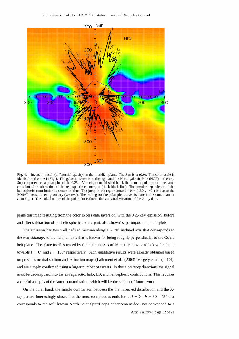
Fig. 4. Inversion result (differential opacity) in the meridian plane. The Sun is at (0,0).The color scale isidentical to the one in Fig 1. The galactic center is to the right and the North galactic Pole (NGP) to the top.Superimposed are a polar plot of the 0.25 keV background (dashed black line), and a polar plot of the sameemission after subtraction of the heliospheric counterpart (thick black line). The angular dependence of theheliospheric contribution is shown in blue. The jump in the region aroundl, b = (180◦,−40◦) is due to theROSAT measurement geometry (see text). The scaling for the polar plot curves is done in the same manneras in Fig. 1. The spiked nature of the polar plot is due to the statistical variation of the X-ray data.

plane dust map resulting from the color excess data inversion, with the 0.25 keV emission (before

and after subtraction of the heliospheric counterpart, also shown) superimposed in polar plots.

The emission has two well defined maxima along a∼ 70◦ inclined axis that corresponds to

the twochimneys to the halo, an axis that is known for being roughly perpendicular to the Gould

belt plane. The plane itself is traced by the main masses of ISmatter above and below the Plane

towardsl = 0◦ and l = 180◦ respectively. Such qualitative results were already obtained based

on previous neutral sodium and extinction maps (Lallement et al. (2003); Vergely et al. (2010)),

and are simply confirmed using a larger number of targets. In thosechimney directions the signal

must be decomposed into the extragalactic, halo, LB, and heliospheric contributions. This requires

a careful analysis of the latter contamination, which will be the subject of future work.

On the other hand, the simple comparison between the the improved distribution and the X-

ray pattern interestingly shows that the most conspicuous emission atl = 0◦, b ≃ 60− 75◦ that

corresponds to the well known North Polar Spur/Loop1 enhancement does not correspond to a



particular nearby (. 300 pc) cavity. This lack of apparent nearby counterpart suggests a distant

emission or a different emission mechanism for the NPS arch. We come back to this point in the

next section that is entirely devoted to the NPS seen in the 0.75 keV range.

3. The 0.75 keV diffuse background and 3D maps: search for the North Polar

Spur (NPS) source region

80

60

40

20

0

-20

-40

-60

-60-40-200204060

-30-18

-501

0203040

30

20

10

NPS

32

1

45-81

0

Fig. 5. ROSAT 0.75 keV surface brightness map around the Galactic Center. Five selected bright regions(dark blue) are labeled and shown. The central parts of thoseregions correspond to the 5 line-of-sight drawnin the four meridional cuts in Fig 6 and the top-right of Fig 7,allowing to correlate visually the bright X-raysources (hot ISM) and low density regions or tunnels appearing in the 3D maps.

3.1. 0.75 keV bright regions in the first and fourth quadrants

Figure 5 illustrates our first study of relationships between X-ray brightness enhancements areas

and voids in the 3D ISM distribution. It shows a large fraction of the 0.75 keV ROSAT map cen-

tered on the GC direction. The 0.75 keV bright regions, in principle, correspond to relatively young

(. 1-2 Myrs) hot ISM bubbles blown by winds from newly born starsand SNRs, and they should

correspond to voids in the 3D ISM distribution. Here, we attempt to use the inverted 3D distribu-

tion to study the correspondency between the bright 0.75 keVdirections and the nearby cavities or

cavity boundaries appearing in the maps. The study has some similarities with HI (or IR) vs X-ray

anti-correlations or shadowing experiments. However herewe use the local ISM distribution and



not quantities integrated up to infinity, and our new approach is fully complementary. Our goal

here is to infer in which way the NPS is similar (or different) from other bright features.

We have selected the main bright regions in the Galactic center region besides the NPS which

are wider than a few degrees, avoidingb . 5◦ region for which the emission is likely to be generated

far outside our mapped volume (e.g., Park et al. (1997)). Numbered 1 to 5 in the following, their

approximate centers arel = 330◦ (-30◦), l = 342◦ (-18◦), l = 355◦ (-5◦) andl = 352◦ (-8◦), and

l = 10◦. They are shown in Fig. 5.

For the first four selected regions, Fig. 6 displays the corresponding planar meridian cuts in

the dust distribution, i.e. meridian planes that contain the central directions of those X-ray bright

areas. The vertical slice corresponding to the fifth bright region atl = 10◦, b = −10◦ to −18◦ is

part of Fig 7. Arrows provide the latitude of the approximatecenters of the bright regions deduced

visually from the ROSAT map. For all five selected bright areas we find in the lower images (Fig.

6 and 7) a corresponding void region in the direction of the bright X-ray emission. The voids have

the forms either of a tunnel linking to empty regions at larger distances, and thus corresponding

to a potential source being located beyond the tunnel, or of anearby cavity, as in the case of the

l = 330◦ enhancement. Such correspondences globally demonstrate aconsistency between the

local IS distribution (despite its poor resolution) and thesoft X-ray maps. Note that interactive 3D

images showing the densest dust structures can be seen at

http://mygepi.obspm.fr/~rlallement/ism3d.html

and

http://mygepi.obspm.fr/~rlallement/ism3dcrevace.html

instead of using the drawn planar cuts.

3.2. Search for a nearby cavity as a source region of the NPS

The North Polar Spur (NPS) is a well-known conspicuous region of strong diffuse X-ray emission,

which coincides in direction with the gigantic radio feature called Loop I. Loop I was recognized

at first as a Galactic giant radio continuum loop of 58◦ ± 4◦ radius centered atl = 329◦ ± 1.5◦ and

b = +17.5◦ ± 3◦ (Berkhuijsen et al. 1971). The bright NPS is centered atl ≈ 30◦ and extends

north aboveb ≈ +10◦. It has been very well mapped in the ROSAT observations (0.1-2.0 keV,

(Snowden et al. 1995)). The NPS is believed to have a local origin, associated to a nearby super-

bubble centered on the Sco-Cen OB associations (∼ 100 pc), the NPS and Loop I corresponding to

the external parts and boundaries of this nearby super-bubble. Some kind of interaction might be

at present between the Local Bubble’s wall in the Galactic center direction and the closest external

region of this super-bubble. At higher latitude, faint filaments seen in HI and extending up to 85◦

also coincide with the radio continuum shells. At least the high latitude Hi filaments in the fourth

quadrant are very close to us. As a matter of fact, using optical spectra, Puspitarini & Lallement

(2012) have set a distance of 98± 6 pc for those low velocity shells. This proximity is in good



agreement with the Loop1-LB scenario. Other HI structures with higher radial velocities and in the

same sky region are located beyond 200 pc.

A contradictory, and indeed completely opposite view is also defended. According to it, the

NPS is a fraction of a super-shell centered at the Galactic center (Bland-Hawthorn & Cohen 2003;

Sofue 2000). More recently, the debate about the distance tothe NPS source region has been

reactivated due to the discovery of the Fermibubbles and associated gamma-ray and microwave

arches associated to the bottom and envelops of the bubbles.As a matter of fact there is a similarity

between the shape of the NPS and arcs seen in gamma rays and microwave that seem to envelop

the northern Fermi bubble. Hence, it is worthwhile to revisit the problem of the location of NPS.

One of the puzzling characteristics of the NPS is its abrupt disappearance belowb = +8◦,

seen in all ROSAT channels. Thus either the source region is extending below this latitude but

is masked by a high column of gas atb . +8◦ (case 1), or the emission is generated only above

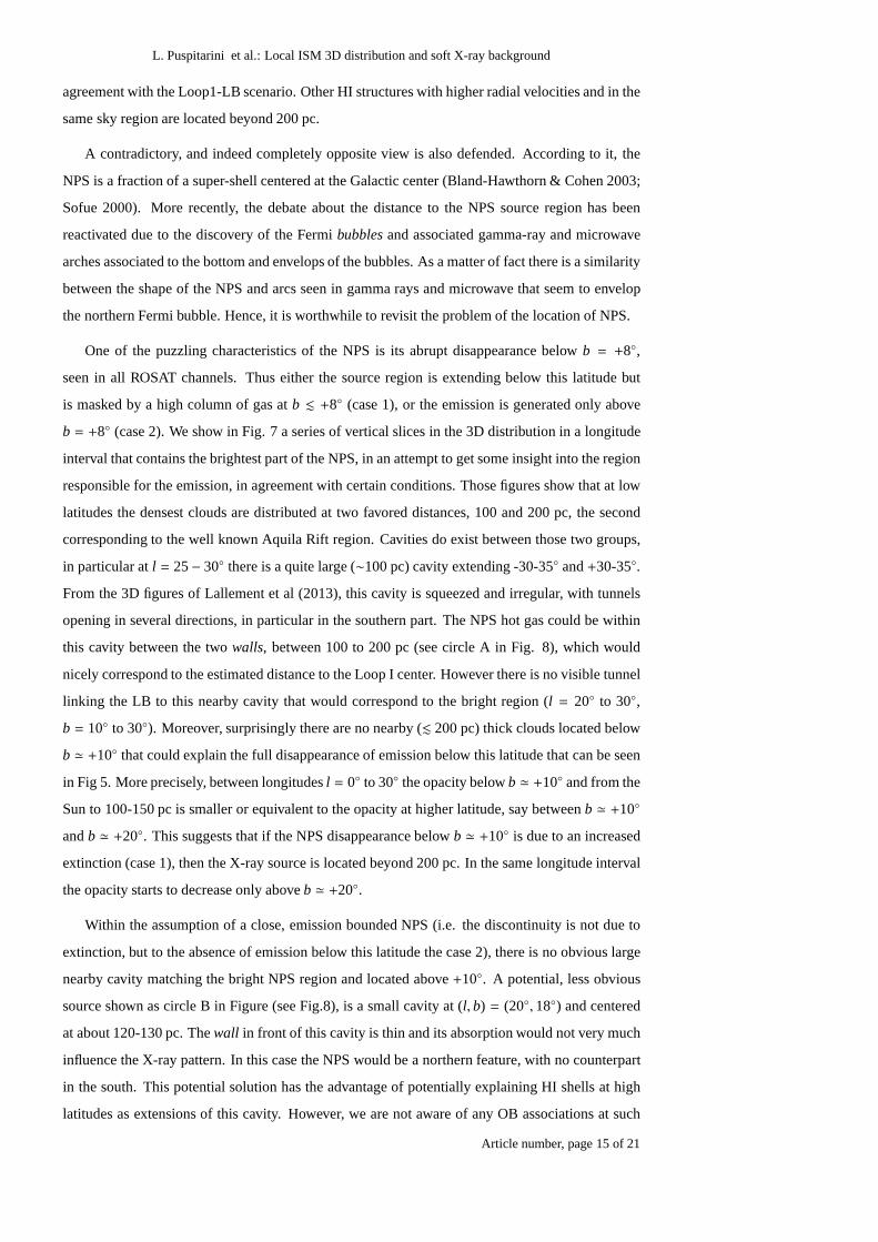
b = +8◦ (case 2). We show in Fig. 7 a series of vertical slices in the 3Ddistribution in a longitude

interval that contains the brightest part of the NPS, in an attempt to get some insight into the region

responsible for the emission, in agreement with certain conditions. Those figures show that at low

latitudes the densest clouds are distributed at two favoreddistances, 100 and 200 pc, the second

corresponding to the well known Aquila Rift region. Cavities do exist between those two groups,

in particular atl = 25− 30◦ there is a quite large (∼100 pc) cavity extending -30-35◦ and+30-35◦.

From the 3D figures of Lallement et al (2013), this cavity is squeezed and irregular, with tunnels

opening in several directions, in particular in the southern part. The NPS hot gas could be within

this cavity between the twowalls, between 100 to 200 pc (see circle A in Fig. 8), which would

nicely correspond to the estimated distance to the Loop I center. However there is no visible tunnel

linking the LB to this nearby cavity that would correspond tothe bright region (l = 20◦ to 30◦,

b = 10◦ to 30◦). Moreover, surprisingly there are no nearby (. 200 pc) thick clouds located below

b ≃ +10◦ that could explain the full disappearance of emission belowthis latitude that can be seen

in Fig 5. More precisely, between longitudesl = 0◦ to 30◦ the opacity belowb ≃ +10◦ and from the

Sun to 100-150 pc is smaller or equivalent to the opacity at higher latitude, say betweenb ≃ +10◦

andb ≃ +20◦. This suggests that if the NPS disappearance belowb ≃ +10◦ is due to an increased

extinction (case 1), then the X-ray source is located beyond200 pc. In the same longitude interval

the opacity starts to decrease only aboveb ≃ +20◦.

Within the assumption of a close, emission bounded NPS (i.e.the discontinuity is not due to

extinction, but to the absence of emission below this latitude the case 2), there is no obvious large

nearby cavity matching the bright NPS region and located above+10◦. A potential, less obvious

source shown as circle B in Figure (see Fig.8), is a small cavity at (l, b) = (20◦, 18◦) and centered

at about 120-130 pc. Thewall in front of this cavity is thin and its absorption would not very much

influence the X-ray pattern. In this case the NPS would be a northern feature, with no counterpart

in the south. This potential solution has the advantage of potentially explaining HI shells at high

latitudes as extensions of this cavity. However, we are not aware of any OB associations at such



latitudes which could potentially have given rise to such a cavity. Also, as we will see in the next

section, absorbing columns derived from X-ray spectra do not match the opacity of the clouds in

front of the cavity. Thus, contrary to the other 5 cases mentioned above, here we could not find

the same type of obvious correspondence between the X-ray pattern and the 3D distribution, if if

distances are restricted to less than 200 pc.

-300

-200

-100

0

100

200

300

5004003002001000

l=-30

NGP

SGP

b=+14¡

-300

-200

-100

0

100

200

300

5004003002001000

20¡

10¡ l=-18¡

NGP

SGP

b=+18¡

-300

-200

-100

0

100

200

300

5004003002001000

l=-5

NGP

SGP

b=+9¡

-300

-200

-100

0

100

200

300

5004003002001000

sun

b=-10¡

NGP

SGP

l=-8

Fig. 6. Inversion results: vertical slices in the 3D distribution at l = −30◦ (case 1),−18◦ (case 2),−5◦ (case3) and−8◦ (case 4). The Sun is at (0,0) in those half-planes. The color scale is identical to the one in Fig 1.The directions of the bright areas labeled in Fig. 5 are shownby a black straight line.

3.3. Inferences from maps and previous NPS spectra

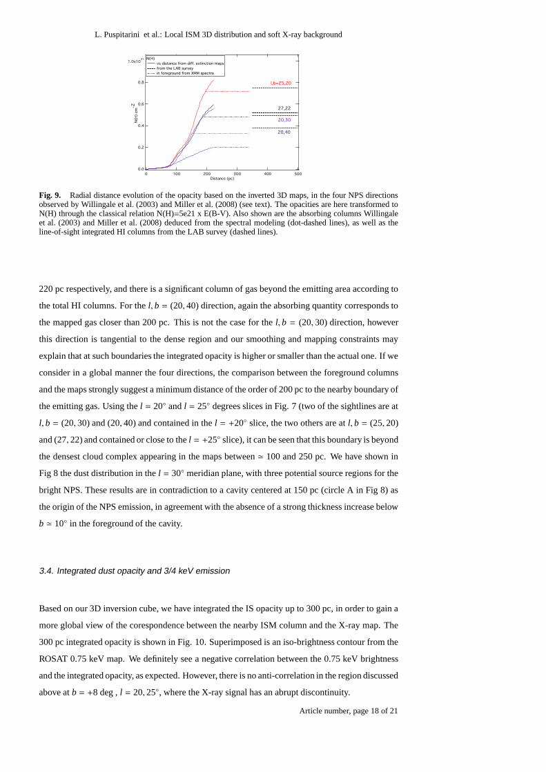
Willingale et al. (2003) and Miller et al. (2008) have analyzed in detail XMM-Newton and Suzaku

spectra towards different directions within the NPS. An output of their spectralmodeling is the

estimated N(H) absorbing column towards the emitting region. We have used our 3D distribution

to integrate the differential opacity along the four directions they have studied. We compare in Fig.

9 those radial opacity profiles with their estimated absorbing columns on one hand, and with the

total HI column deduced from 21 cm data (Kalberla et al. 2005)on the other hand. We caution

here again that the map resolution is of the order of 20-30 pc in this volume, i.e. there is a strong

averaging of the structures that explains the smooth increases in opacity. Another characteristic of

the inversion must also be mentioned here, namely the use of adefault distribution, a distribution

that prevails at locations where there are no constraints from the reddening database. Such a default

distribution has no influence on the location of the mapped clouds, but when computing opacity

integrals there maybe a non negligible influence of this distribution, especially outside the Plane

and at large distances where there are fewer targets. In the maps we use here the default distribution



Fig. 7. Inversion result: vertical slices in the 3D dust distribution containing or around the NPS brightdirections. The color scale is identical to the one in Fig 1. The l = +10◦ slice contains the direction of thebright region number 5 of Fig 5.

-300

-200

-100

0

100

200

300

-400 -200 0 200 400

30,0

b=+90

sun210,0 A

B

C

Ori CO

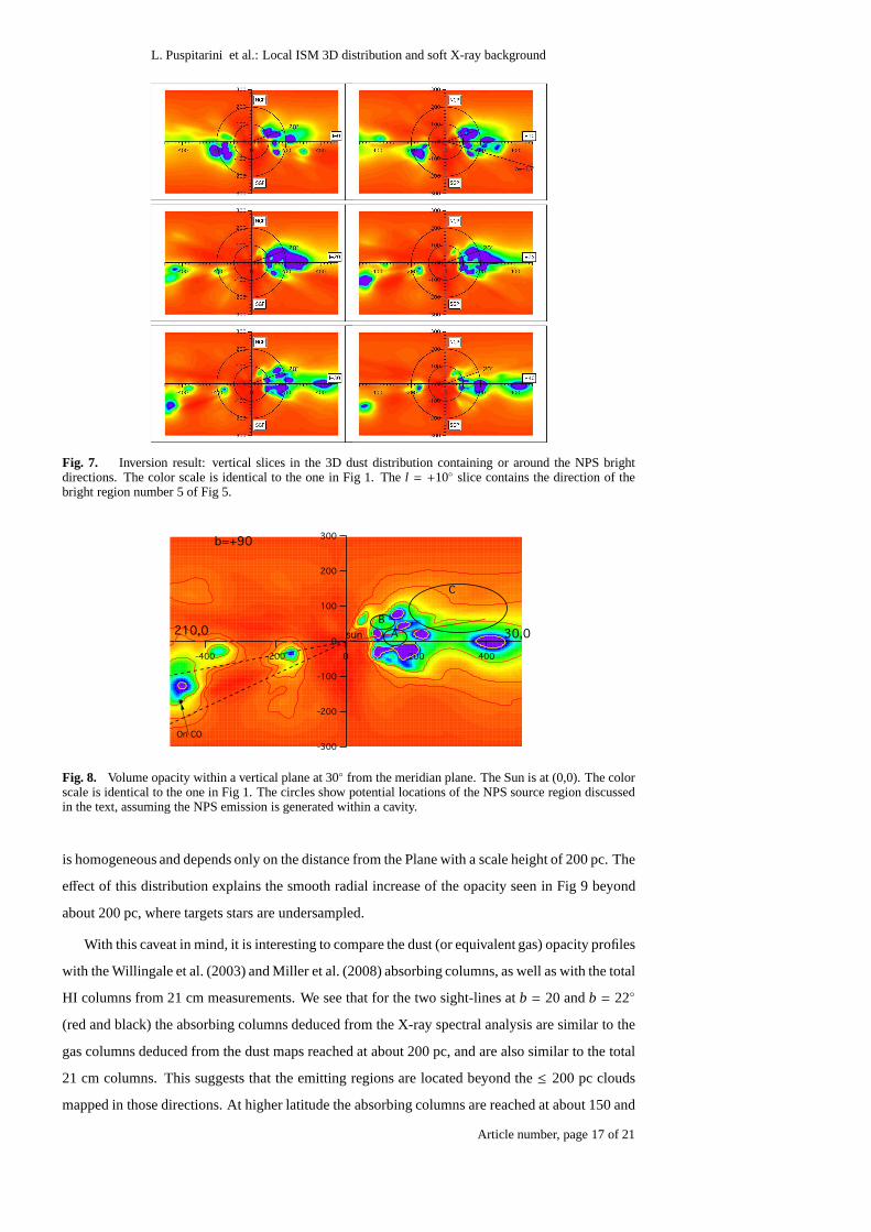
Fig. 8. Volume opacity within a vertical plane at 30◦ from the meridian plane. The Sun is at (0,0). The colorscale is identical to the one in Fig 1. The circles show potential locations of the NPS source region discussedin the text, assuming the NPS emission is generated within a cavity.

is homogeneous and depends only on the distance from the Plane with a scale height of 200 pc. The

effect of this distribution explains the smooth radial increase of the opacity seen in Fig 9 beyond

about 200 pc, where targets stars are undersampled.

With this caveat in mind, it is interesting to compare the dust (or equivalent gas) opacity profiles

with the Willingale et al. (2003) and Miller et al. (2008) absorbing columns, as well as with the total

HI columns from 21 cm measurements. We see that for the two sight-lines atb = 20 andb = 22◦

(red and black) the absorbing columns deduced from the X-rayspectral analysis are similar to the

gas columns deduced from the dust maps reached at about 200 pc, and are also similar to the total

21 cm columns. This suggests that the emitting regions are located beyond the≤ 200 pc clouds

mapped in those directions. At higher latitude the absorbing columns are reached at about 150 and



1.0x1021

0.8

0.6

0.4

0.2

0.0

N(H

) cm

-2

5004003002001000Distance (pc)

l,b=25,20

27,22

20,30

20,40

N(H)

vs distance from diff. extinction maps

from the LAB survey

in foreground from XMM spectra

Fig. 9. Radial distance evolution of the opacity based on the inverted 3D maps, in the four NPS directionsobserved by Willingale et al. (2003) and Miller et al. (2008)(see text). The opacities are here transformed toN(H) through the classical relation N(H)=5e21 x E(B-V). Also shown are the absorbing columns Willingaleet al. (2003) and Miller et al. (2008) deduced from the spectral modeling (dot-dashed lines), as well as theline-of-sight integrated HI columns from the LAB survey (dashed lines).

220 pc respectively, and there is a significant column of gas beyond the emitting area according to

the total HI columns. For thel, b = (20, 40) direction, again the absorbing quantity corresponds to

the mapped gas closer than 200 pc. This is not the case for thel, b = (20, 30) direction, however

this direction is tangential to the dense region and our smoothing and mapping constraints may

explain that at such boundaries the integrated opacity is higher or smaller than the actual one. If we

consider in a global manner the four directions, the comparison between the foreground columns

and the maps strongly suggest a minimum distance of the orderof 200 pc to the nearby boundary of

the emitting gas. Using thel = 20◦ andl = 25◦ degrees slices in Fig. 7 (two of the sightlines are at

l, b = (20, 30) and (20, 40) and contained in thel = +20◦ slice, the two others are atl, b = (25, 20)

and (27, 22) and contained or close to thel = +25◦ slice), it can be seen that this boundary is beyond

the densest cloud complex appearing in the maps between≃ 100 and 250 pc. We have shown in

Fig 8 the dust distribution in thel = 30◦ meridian plane, with three potential source regions for the

bright NPS. These results are in contradiction to a cavity centered at 150 pc (circle A in Fig 8) as

the origin of the NPS emission, in agreement with the absenceof a strong thickness increase below

b ≃ 10◦ in the foreground of the cavity.

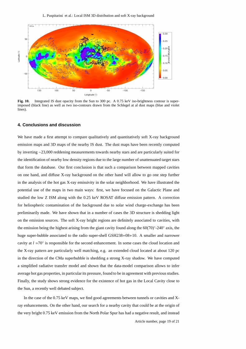
3.4. Integrated dust opacity and 3/4 keV emission

Based on our 3D inversion cube, we have integrated the IS opacity up to 300 pc, in order to gain a

more global view of the corespondence between the nearby ISMcolumn and the X-ray map. The

300 pc integrated opacity is shown in Fig. 10. Superimposed is an iso-brightness contour from the

ROSAT 0.75 keV map. We definitely see a negative correlation between the 0.75 keV brightness

and the integrated opacity, as expected. However, there is no anti-correlation in the region discussed

above atb = +8 deg ,l = 20, 25◦, where the X-ray signal has an abrupt discontinuity.



-50

0

50

Lati

tude (

¡)

150 100 50 0 -50 -100 -150

Longitude (¡)

300 pc

0.30

0.25

0.20

0.15

0.10

0.05

0.00in

tegra

ted d

ensity

Fig. 10. Integrated IS dust opacity from the Sun to 300 pc. A 0.75 keV iso-brightness contour is super-imposed (black line) as well as two iso-contours drawn from the Schlegel at al dust maps (blue and violetlines).

4. Conclusions and discussion

We have made a first attempt to compare qualitatively and quantitatively soft X-ray background

emission maps and 3D maps of the nearby IS dust. The dust maps have been recently computed

by inverting∼23,000 reddening measurements towards nearby stars and areparticularly suited for

the identification of nearby low density regions due to the large number of unattenuated target stars

that form the database. Our first conclusion is that such a comparison between mapped cavities

on one hand, and diffuse X-ray background on the other hand will allow to go one step further

in the analysis of the hot gas X-ray emissivity in the solar neighborhood. We have illustrated the

potential use of the maps in two main ways: first, we have focused on the Galactic Plane and

studied the low Z ISM along with the 0.25 keV ROSAT diffuse emission pattern. A correction

for heliospheric contamination of the background due to solar wind charge-exchange has been

preliminarily made. We have shown that in a number of cases the 3D structure is shedding light

on the emission sources. The soft X-ray bright regions are definitely associated to cavities, with

the emission being the highest arising from the giant cavityfound along the 60(70)◦-240◦ axis, the

huge super-bubble associated to the radio super-shell GSH238+08+10. A smaller and narrower

cavity atl ≃70◦ is responsible for the second enhancement. In some cases thecloud location and

the X-ray pattern are particularly well matching, e.g. an extended cloud located at about 120 pc

in the direction of the CMa superbubble is shedding a strong X-ray shadow. We have computed

a simplified radiative transfer model and shown that the data-model comparison allows to infer

average hot gas properties, in particular its pressure, found to be in agreement with previous studies.

Finally, the study shows strong evidence for the existence of hot gas in the Local Cavity close to

the Sun, a recently well debated subject.

In the case of the 0.75 keV maps, we find good agreements between tunnels or cavities and X-

ray enhancements. On the other hand, our search for a nearby cavity that could be at the origin of

the very bright 0.75 keV emission from the North Polar Spur has had a negative result, and instead



we find evidence that the NPS signal originates from hot gas beyond 200 pc, at a larger distance

than previously inferred. The same conclusion is reached from the comparison between the mapped

dust distribution and foreground absorbing columns deduced from NPS X-ray spectra. Since we

derive a lower limit, a much larger distance, including the Galactic center, is not precluded.

More detailed maps are required to improve such types of diagnostics of the emitting regions,

in particular in the case of the NPS for which there is no definite answer here. Hopefully increas-

ing numbers of target stars will allow to built such maps and reveal more detailed IS structures.

Numerous spectra and subsequently large datasets of individual IS absorption and extinction mea-

surements are expected from spectroscopic surveys with Multi-Object spectrographs (MOS). In

parallel, precise parallactic distances will hopefully beprovided by the ESA cornerstone GAIA

mission.

Acknowledgements.

References

de Avillez, M. A., & Breitschwerdt, D. 2009, ApJ, 697, L158

Berkhuijsen, E. M., Haslam, C. G. T., & Salter, C. J. 1971, A&A, 14, 252

Bland-Hawthorn, J., & Cohen, M. 2003, ApJ, 582, 246

Cravens, T. E. 2000, ApJ, 532, L153

Egger, R. J., & Aschenbach, B. 1995, A&A, 294, L25

Freyberg, M. J. 1994, Ph.D. Thesis,

Fujimoto, R., Mitsuda, K., Mccammon, D., et al. 2007, PASJ, 59, 133

Gry, C., York, D. G., & Vidal-Madjar, A. 1985, ApJ, 296, 593

Haslam, C. G. T., Large, M. I., & Quigley, M. J. S. 1964, MNRAS,127, 273

Heiles, C. 1998, ApJ, 498, 689

Kalberla, P. M. W., Burton, W. B., Hartmann, D., et al. 2005, A&A, 440, 775

Koutroumpa, D., Acero, F., Lallement, R., Ballet, J., & Kharchenko, V. 2007, A&A, 475, 901

Koutroumpa, D., Lallement, R., Raymond, J. C., & Kharchenko, V. 2009a, ApJ, 696, 1517

Koutroumpa, D., Collier, M. R., Kuntz, K. D., Lallement, R.,& Snowden, S. L. 2009b, ApJ, 697, 1214

Lallement, R., Welsh, B. Y., Vergely, J. L., Crifo, F., & Sfeir, D. 2003, A&A, 411, 447

Lallement, R. 2004, A&A, 418, 143

Lallement, R., Vergely, J. L., Valette B., Puspitarini L., Eyer L., Casagrande L. 2013, A&A, in press

Miller, E. D., Tsunemi Hiroshi, Bautz, M. W., et al. 2008, PASJ, 60, 95

Park, S., Finley, J. P., Snowden, S. L., & Dame, T. M. 1997, ApJ, 476, L77

Puspitarini, L., & Lallement, R. 2012, A&A, 545, A21

Raymond, J. C., & Smith, B. W. 1977, ApJS, 35, 419

Redfield, S., & Linsky, J. L. 2000, ApJ, 534, 825

Schlegel, D. J., Finkbeiner, D. P., & Davis, M. 1998, ApJ, 500, 525

Snowden, S. L., Freyberg, M. J., Plucinsky, P. P., et al. 1995, ApJ, 454, 643

Snowden, S. L., Egger, R., Freyberg, M. J., et al. 1997, ApJ, 485, 125

Snowden, S. L. 1998, ApJS, 117, 233

Snowden, S. L. 1998, IAU Colloq. 166: The Local Bubble and Beyond, 506, 103

Snowden, S. L., Egger, R., Finkbeiner, D. P., Freyberg, M. J., & Plucinsky, P. P. 1998, ApJ, 493, 715

Snowden, S. L., Freyberg, M. J., Kuntz, K. D., & Sanders, W. T.2000, ApJS, 128, 171

Snowden, S. L., Collier, M. R., & Kuntz, K. D. 2004, ApJ, 610, 1182



Sofue, Y. 2000, ApJ, 540, 224

Tarantola, A., & Valette, B. 1982, Reviews of Geophysics andSpace Physics, 20, 219

Vergely, J.-L., Freire Ferrero, R., Siebert, A., & Valette,B. 2001, A&A, 366, 1016

Vergely, J.-L., Valette, B., Lallement, R., & Raimond, S. 2010, A&A, 518, A31

Wargelin, B. J., Markevitch, M., Juda, M., et al. 2004, ApJ, 607, 596

Welsh, B. Y., Lallement, R., Vergely, J.-L., & Raimond, S. 2010, A&A, 510, A54

Willingale, R., Hands, A. D. P., Warwick, R. S., Snowden, S. L., & Burrows, D. N. 2003, MNRAS, 343, 995

Wolleben, M., 2007, ApJ, 664, 349

Wolff, B., Koester, D., & Lallement, R. 1999, A&A, 346, 969

List of Objects


Local ISM 3D distribution and soft X-ray background · PDF file · 2015-01-133 Code...

Documents

Transcript of Local ISM 3D distribution and soft X-ray background · PDF file · 2015-01-133 Code...