Local Feature Analysis: A Statistical Theory for Reproducible

Local Feature Analysis: A Statistical Theory forReproducible Essential Dynamics of Large MacromoleculesZhiyong Zhang, and Willy Wriggers*Laboratories for Biocomputing & Imaging, School of Health Information Sciences & Institute of Molecular Medicine, Universityof Texas Health Science Center at Houston, Houston, Texas

ABSTRACT Multivariate statistical methodsare widely used to extract functional collectivemotions from macromolecular molecular dynamics(MD) simulations. In principal component analysis(PCA), a covariance matrix of positional fluctua-tions is diagonalized to obtain orthogonal eigenvec-tors and corresponding eigenvalues. The first feweigenvectors usually correspond to collective modesthat approximate the functional motions in theprotein. However, PCA representations are globallycoherent by definition and, for a large biomolecularsystem, do not converge on the time scales acces-sible to MD. Also, the forced orthogonalization ofmodes leads to complex dependencies that are notnecessarily consistent with the symmetry of biologi-cal macromolecules and assemblies. Here, we de-scribe for the first time the application of localfeature analysis (LFA) to construct a topographicrepresentation of functional dynamics in terms oflocal features. The LFA representations are lowdimensional, and like PCA provide a reduced basisset for collective motions, but they are sparselydistributed and spatially localized. This yields amore reliable assignment of essential dynamicsmodes across different MD time windows. Also, theintrinsic dynamics of local domains is more exten-sively sampled than that of globally coherent PCAmodes. Proteins 2006;64:391–403.© 2006 Wiley-Liss, Inc.

Key words: principal component analysis; local fea-ture analysis; molecular dynamics; bac-teriophage T4 lysozyme; functional do-main motions

INTRODUCTION

Molecular dynamics (MD) is an important tool in thestudy of the functional dynamics of proteins and macromo-lecular complexes.1,2 One of the major limitations of MD isthe shortness of achievable simulation times, typically ofthe order of tens to hundreds of nanoseconds. These timesare much shorter than the time scales of many importantbiological processes, such as multidomain motions andallosteric transitions, that take place on the millisecondscale and beyond.3,4 Therefore, attempts have been madeto extract ‘essential’ functional features from the shorttrajectories, with the hope to describe the motion in termsof a small number of variables, sometimes called collectivecoordinates or essential degrees of freedom.5–11

One widely used statistical approach to such dimension-ality reduction is principal component analysis (PCA),12,13

also known as the Karhunen–Loeve expansion14 in timeseries analysis. This statistical method was introduced tothe protein research community by McCammon, Karplus,and their coworkers15,16 in the 1980s under the namequasi-harmonic analysis. Since the early 1990s, PCA-based essential dynamics techniques have enjoyed theincreasing enthusiasm of a large number of investiga-tors7,8 who successfully applied them to investigate thephysical nature of protein dynamics and to sample theconformational space.10,11

While there is general agreement about the heuristicappeal of PCA for the prediction of functionally relevantmodes, it became necessary in the mid-1990s to investi-gate the limitations of PCA conferred by the MD samplingproblem. Garcıa and colleagues demonstrated that forlarge systems the distribution of conformations becomesmultimodal9 (as suggested also by Go’s jumping-among-minima model17), leading to a breakdown of the quasi-harmonic assumption. Also, Clarage and colleagues showedthat correlations in low-frequency displacements are un-der sampled by nanosecond MD simulations and asked thequestion “How long is long enough?”18 An answer may befound in experimental studies that suggest that the relax-ation times of correlations for multidomain proteins are onthe order of milliseconds or longer.3,4 This led Balsera andcoworkers to conclude that PCA modes from short MDtrajectories are intrinsically unreliable.19

Here, we take the conciliatory view that PCA may serveas a useful filter for identifying a reduced dimensional, oressential subspace, although it is clear from the prior workthat individual PCA modes may overestimate the coher-ence of long-distance motions due to limited sampling anddue to the global extent of the modes. The PCA filteringenables a subsequent local representation of the dynamics

Grant sponsor: NIH; Grant numbers: 1R01GM62968,1R90DK071505-01; Grant sponsor: Human Frontier Science Pro-gram; Grant number: RGP0026/2003; Grant sponsor: Alfred P.Sloan Foundation; Grant number: BR-4297.

*Correspondence to: Willy Wriggers, Laboratories for Biocomputing& Imaging, School of Health Information Sciences & Institute ofMolecular Medicine, University of Texas Health Science Center atHouston, 7000 Fannin St., Suite 600, Houston, TX 77030. E-mail:[email protected]

Received 13 October 2005; 18 January 2006; 7 February 2006

Published online 12 May 2006 in Wiley InterScience(www.interscience.wiley.com). DOI: 10.1002/prot.20983

PROTEINS: Structure, Function, and Bioinformatics 64:391–403 (2006)

© 2006 WILEY-LISS, INC.

described below. In this filtering role of PCA, it is notnecessary to know a priori which particular PCA mode(or which linear combination of modes) is functionallyrelevant. Our minimal assumption is that only the com-bined subspace is relevant, as suggested by the findings ofAmadei and colleagues7 and by a recent survey of har-monic (or normal mode) analysis of protein dynamics,where observed conformational changes are most oftencontained within the subspace of the first 12 low-frequencymodes.20

The global extent of individual PCA modes is problem-atic not only because of the limited sampling of long-rangecorrelations, but also because of the forced orthogonaliza-tion of the modes. Since the nth mode is always forced to beorthogonal to the first n � 1 modes, complex causaldependencies arise. For example, one can not claim that aparticular mode n is functionally isolated from (or lessrelevant than) slower modes. In Balsera’s paper,19 it wasshown that even fast modes, whose relaxation time is wellwithin the MD sampling window, cannot be recovered byPCA due to their dependence on the slower, undersampledmodes. The forced orthogonalization also has the undesir-able effect of breaking the symmetry of large-scale macro-molecular assemblies. For example, a three-fold symmet-ric system should exhibit a symmetry relatedrepresentation (for each 120° rotation), instead PCA fixesby numeric chance one of the three possible solutions andforces all subsequent modes to be orthogonal, therebybreaking the symmetry.

Due to the apparent limitations of global collectivecoordinates, we were seeking an alternative statisticaltheory that describes dynamic features locally and thatdoes not suffer from the sampling and orthogonalizationproblems. A particularly promising recent approach isnon-negative matrix factorization (NMF)21,22 of imagedata, which has been used for classification tasks in facerecognition. Compared to the global PCA representation(eigenfaces), the NMF basis corresponds to recognizablelocalized features such as parts of a face (eyes, nose, ears,and mouth). Instead of the forced orthogonalization as inPCA, NMF uses non-negativity constraints in the matrixfactorization, which lead to a parts-based representationof the objects. Unfortunately, this promising concept is notapplicable to protein dynamics, as the elements in thecovariance matrix could have either sign and can not berestricted to positive values as in gray value images.

Earlier, Penev and Atick developed an alternative statis-tical technique, termed local feature analysis (LFA), toconstruct a local topographic representation of objectsfrom the global PCA modes.23 It turns out that LFA is freefrom non-negativity constraints, although this was notexploited at the time. As in the case of NMF the LFA basisfunctions are sparsely distributed and give a description ofobjects in terms of local features and their positions. Inthis article, we adapted for the first time the theoreticalframework of LFA to the study of protein dynamics. Weobtained local features that clearly correspond to seg-mented dynamic domains in the protein. Also, LFA pro-

vides for a significant improvement in the reproducibilityand convergence of the statistical sampling.

The organization of this paper is as follows. Firstly wewill describe our adaptation of the theory of LFA, as wellas computational details for the MD simulation of a testsystem, bacteriophage T4 lysozyme (T4L). Subsequently,we provide results and a discussion regarding the perfor-mance features of LFA. Finally, we provide concludingremarks on the parameterization and future applicabilityof the algorithm.

THEORY AND METHODSLocal Representations from PCA Modes

Assuming a protein structure, for simplicity we onlyconsider here the coordinates of a number N C� atoms.Amadei and colleagues demonstrated that the identity ofthe larger amplitude modes is robust under such C� coarsegraining.7,24 A generalization to all atoms is straightfor-ward. After eliminating the overall translational androtational motion from the MD simulation as is customaryin PCA, the internal motion is described by a trajectoryx(t), where x is a 3N-dimensional column vector of the C�atomic coordinates: {x1, x2, . . ., x3N}. The correlations ofatomic fluctuations are expressed in a covariance matrix

C�i, j� � ��xi�xj� � ��xi � �xi�� xj � �xj��, (1)

where �� denotes an average over the time frames. In PCA,we diagonalize the covariance matrix to produce theorthogonal set of eigenvectors (PCA modes) �r(i), r 1, . . .,3N and corresponding eigenvalues r:

C�i, j� � �r 1

3N

�r�i�r�r�j�. (2)

The displacements �xi can then be reconstructed from thePCA modes

�xi � �r 1

3N

Ar�r�i� with Ar � �i 1

3N

�r�i��xi � �i 1

3N

Kr�i��xi,

(3)

where Ar is the so-called output of the representation, thatis, the projection of atomic fluctuations onto the PCA mode�r. PCA outputs are decorrelated in the sense that �ArAq� r�rq. Kr(i) is the so-called kernel of the PCA representa-tion, in the case of PCA Kr(i) �r(i). We choose to sort r ina decreasing order, thus the first eigenvector represent themotion that has the largest positional deviation. As ex-plained above, we assume that a small number n(n �� 3N)of modes are sufficient to describe the dominant dynamics.This means we truncate the expansion (Eq. 3) early anddefine the (approximate) reconstructed deviations:

�xirec � �

r 1

n

Ar�r�i�. (4)

The PCA representation offers a reduced dimensionality,however, it is nonlocal. By this we mean that the kernel

PROTEINS: Structure, Function, and Bioinformatics DOI 10.1002/prot

392 Z. ZHANG AND W. WRIGGERS

functions Kr(i) (Eq. 3) extend over the entire range of i (the3N degrees of freedom of the protein), but nearby values inthe r index have no relationship among each other. For thedesired LFA, we recast the expansion into a new represen-tation that obeys locality, that is, the kernel functions arenot labeled by the PCA mode index r, but by the index ofthe degrees of freedom (DOF), i. The most general form forthe LFA kernel is

K�i, j� � �r, s 1

n

�r�i�Qrs�s�j�, (5)

where Qrs is an arbitrary matrix. Similar to the PCAoutputs Ar in Equation 3, we define local outputs O(i)

O�i� � �j 1

3N

K�i, j��xj � �r, s 1

n

�r�i�QrsAs, (6)

but here O depends on i and not on r. We know that thePCA outputs Ar are decorrelated by frequency, so likewisewe seek to decorrelate the local outputs O(i) by space.Because the 3N outputs O(i) are derived from only n �� 3Nlinearly independent Ar, the decorrelation condition�O(i)O(j)� �(i, j) is no longer satisfied. Instead we seek tosatisfy the condition of minimum correlation of the outputsO(i) by minimizing the mean-square deviation

msd � �i, j 1

3N

��O�i�O�j�� i, j)�2 (7)

with respect to the matrix Q. One can show that Q must be

given by Qrs 1

�rUrs,

23 and Urs is any orthogonal matrix

satisfying UTU 1. In general, a variety of Urs may beemployed while preserving the decorrelation,25 but here

Fig. 1. Sparsification results of T4L. The first n PCA modes were used to perform LFA: (a) n 4; (b) n 8;(c) n 12; (d) n 15. The selected C� atoms are represented by spheres. Red–green–blue colors indicate theorder of selection by the algorithm (the first selected C� atom is red, and the last one is blue). (e)Root-mean-square fluctuations (RMSF) of C� atoms in T4L. Trajectory frames from 2 to 10 ns were used tocalculate the RMSF. Four seed atoms (C� � 21, C� � 52, C� � 109, and C� � 127) are indicated by black dots.


LOCAL FEATURE ANALYSIS 393

we consider only the simplest choice Urs �rs to remainconsistent with the PCA subspace. Thus, according toEquation 6 the LFA outputs become

O�i� � �j 1

3N � �r 1

n

�r�i�1

�r�r�j�� xj � �

r 1

n Ar

�r�r�i�

(8)

and their residual correlation is given by

�O�i�O�j�� r 1

n

�r�i��r�j� � P�i, j�. (9)

In the limit n 3 3N the LFA outputs are completelydecorrelated: P(i, j) 3 �(i, j). Finally, we have derived anew kernel function

K�i, j� � �r 1

n

�r�i�1

�r�r�j�, (10)

which satisfies locality. We reconstruct �xi using thesekernels.

The matrices K and P are central to LFA and one canderive from the above equations some additional notewor-thy features. First, K is by definition the projection opera-tor onto a local feature. In the limit n3 3N, the resultingdimensionless projections (or outputs) O(i) become orthogo-nal, as well as normalized to unity, as square-integrable

functions over the time domain. Second, it is straightfor-ward to show from Equations 4 and 9 that

�j 1

3N

P�i, j��xj � �xirec. (11)

This means that P serves a dual role both as the correla-tion of the results of K (the LFA outputs) and as theprojection operator onto the low-frequency subspacespanned by n PCA modes. Used as a projection operatorthe results of P then have length units (unlike the resultsof K that are dimensionless). Third, from Equations 4 and8 we get

�xirec � �

j 1

3N

K��1��i, j�O�j�, (12)

where K(�1) �r1

n �r(i)�r�r(j) is the so-called reconstruc-

tor or inverse kernel of the representation.In summary, the above LFA theory can be formulated in

a compact form as follows. If we define a family of functions

K(m)(i, j) �r1

n �r(i) � 1

�r�m

�r(j), then it follows that

K(1)(i,j) K(i, j) is the LFA kernel (Eq. 10); K(0)(i, j) P(i, j) is the residual output correlation (Eq. 9); K(�1)(i, j) isthe reconstructor (Eq. 12); and K(�2)(i, j) C(i, j) is thecovariance matrix (Eq. 2).

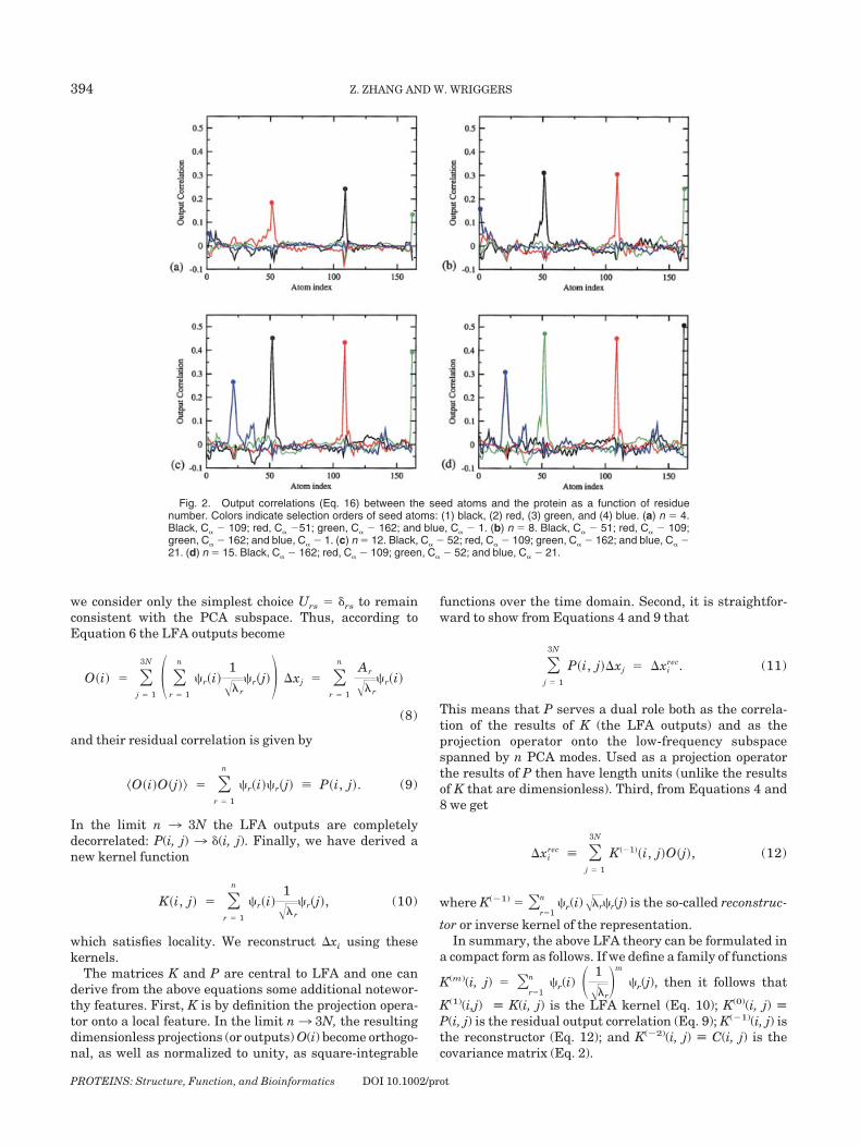
Fig. 2. Output correlations (Eq. 16) between the seed atoms and the protein as a function of residuenumber. Colors indicate selection orders of seed atoms: (1) black, (2) red, (3) green, and (4) blue. (a) n 4.Black, C� � 109; red, C� �51; green, C� � 162; and blue, C� � 1. (b) n 8. Black, C� � 51; red, C� � 109;green, C� � 162; and blue, C� � 1. (c) n 12. Black, C� � 52; red, C� � 109; green, C� � 162; and blue, C� �21. (d) n 15. Black, C� � 162; red, C� � 109; green, C� � 52; and blue, C� � 21.



Sparsification from Local Features

In the previous section, we replaced the n global PCAmodes with a much larger number 3N of local LFA outputfunctions O(i). Although locality was achieved, it came at aprice of expanding again to the full number of DOF.Therefore, an additional dimensionality reduction step isrequired in the LFA output space. This sparsificationtakes advantage of the fact that neighboring outputs arehighly correlated. We approximate the entire 3N outputsO(i) with only a small subset of {O(im)}i,m�� that corre-spond to the strongest local features. The other O(i) canthen be reasonably well predicted via the correlations P(i,im) Pm(i).

We begin with an empty set �(0) {0}. At each step, outof the 3N total DOF we add a seed index to �, chosenaccording to the criteria described below, the seed indexcorresponds to either x, y, or z, coordinates of a given seedatom. Given the current set �(m), we can reconstruct theoutputs:

Orec�i� � �m 1

��

am(i)O(im). (13)

One can show23 that the optimal linear prediction coeffi-cients am(i), defined to minimize the average reconstruc-tion mean square error on O(i)

Erec � ��Oerr�i��2� � ��O�i� � Orec�i��2�, (14)

are given by

am�i� � �l 1

��

P�i, il��P��1�lm, (15)

where P��1 is the inverse of a submatrix P� from P: P�lm P(il, im). Out of the 3N available DOF we chose the seedindex that has the maximum reconstruction error Oerr(im �

1) as the (m � 1)th index into �, under the condition thatthe seed atom and its nearest neighbors are distinct fromatoms corresponding to previously found indices. We keepadding seed indices to � until n indices are chosen (theentire set of O(i) is reconstructed without error at thistime).

In principle, any n seed indices can recover the O(i)without error. However, if we choose indices whose P(i, j)overlap significantly, the {O(im)}im�� will be correlated andthe representation would be redundant in some regionsbut insufficient in other regions. In the above sparsifica-tion algorithm, we choose an index whose output is pre-dicted worst by the already chosen ones. This assures thatthe corresponding atom is dynamically decorrelated fromthe atoms corresponding to already chosen indices.

COMPUTATIONAL DETAILS

The MD simulation and some of the subsequent analysiswere performed using the GROMACS package (version3.1.4), using the GROMACS forcefield with united-atommodel.26,27 We selected bacteriophage T4 lysozyme (T4L)as a test system. T4L is composed of two domains con-

nected by a long �-helix, there is a deep opening betweenthe N-terminal and C-terminal domains, which is theactive-site cleft.28 There are many experimental struc-tures of T4L and its mutants that indicate a hinge-bending–type domain motion.29,30

The crystal structure of T4L (PDB entry:2LZM) deter-mined at 1.7 A resolution was used as the startingstructure.31 Rectangular periodic boundary conditions wereused with box length of 6.356 nm � 6.287 nm � 7.303 nm(the minimum distance between the solute and the boxboundary is 1.2 nm). SPC water molecules were addedfrom an equilibrated cubic box containing 216 watermolecules.32 The system, protein and water, was initiallyenergy-minimized using the steepest descent method,until the maximum force on the atoms is smaller than1000 kJ mol�1 nm�1. Eight Cl� ions were added tocompensate the net positive charge on the protein, andthese ions were introduced by replacing water moleculeswith the most favorable electrostatic potential. The energywas again minimized using the conjugate gradient algo-rithm, until the maximum force is below 200 kJ mol�1

Fig. 3. T4L structures colored by output correlations (Eq. 16) betweenthe seed atom (represented by a blue sphere) and other C� atoms. Blueindicates positive, white indicates 0, and red indicates negative correla-tion values. n 4 PCA modes were used for LFA, and the four seedatoms are shown by in order of selection. (a) C� � 109, (b) C� � 51, (c)C� � 162, and (d) C� � 1.



nm�1. The final system contains 1683 protein atoms, 8 Cl�

ions, and 8775 water molecules, leading to a total size of28,016 atoms. A 100 ps positional-restraint equilibrationsimulation was performed, with force constants 1000 kJmol�1 nm�2, and then followed by a 10 ns production run.The last 8 ns of this run were used to perform PCA.

We used an isothermal–isobaric simulation algorithm.33

The three groups (protein, ions, and solvent) were coupledseparately to a temperature bath of reference temperature300 K (relaxation time 0.1 ps). The pressure was also keptconstant by weak coupling to a reference value P0 1 bar(relaxation time 1.0 ps). Covalent bonds in the proteinwere constrained using the LINCS algorithm.34 van derWaals interactions were treated using twin-range cutoffradii (0.9 nm and 1.4 nm), and the pairlist was updatedevery 10 fs. The long-range electrostatic interactions wereevaluated by using the particle mesh Ewald (PME)method35 with a PME tolerance of 10�5 and a PMEinterpolation order of 4.

RESULTS AND DISCUSSIONLocal Dynamic Domains in T4 Lysozyme

The first n 4, 8, 12, and 15 PCA modes were used toconstruct the LFA matrices P(i, j) (Eq. 9) and K(i, j) (Eq.10). This was followed by the sparsification algorithmdescribed above to select n seed atoms. Results are visual-ized using VMD36 (Fig. 1). The location and the order of theselected atoms indicate that they are allocated predomi-nantly at the most flexible regions of the protein, in closeagreements with the peaks of the root-mean-square fluctua-tions (RMSF) of C� atoms [Fig. 1(e)]. The flexible N-terminal and C-terminal atoms are selected in the fourcases (Fig. 1) owing to their structural variability. Otherseed atoms, such as C� � 21, C� � 52, C� � 109, and C� �127 are also selected frequently (Fig. 1) for a largernumber of seed atoms selected. The functional motion ofthese regions is interpreted in more detail below.

We intend to represent a local feature by one seed atomand its neighboring correlated region (dynamic domain).Considering a seed atom h, its LFA output (O� h) has three

Fig. 4. Locations and dynamics ofthe local features in T4L during thesimulation. (a) Initial structure of thesimulation (t 0 ns), (b) t 4.00 ns,and (c) t 8.25 ns. The first 15 PCAmodes were used for LFA (n 15).Four local features are colored by red(C� � 109), green (C� � 52), blue(C� � 21), and purple (C� � 127),respectively. Seed atoms are repre-sented by spheres. The white cartoonrepresentation indicates the second-ary structure elements.

Fig. 5. (a) Two-dimensional projections of T4L structures from thePDB and of the MD trajectory frames onto the subspace defined by theclosure and twist modes. Thirtyeight crystal structures are indicated asblack dots. The extreme open (PDB entry: 178L) and closed (PDB entry:152L) structures are labeled. Trajectory frames (see text) are shown asbrown dots, except for the configurations at t 0 ns, t 4.00 ns, and t 8.25 ns that are emphasized by red, green, and blue dots, respectively.(b) The open structure (PDB entry: 178L), and (c) the closed structure(PDB entry: 152L), with local features from the MD simulation highlightedas in Figure 4.



components: O(hd), d 1, 2, or 3. The correlation betweenthe seed atom and any other atom k (with LFA output O� k)is:

�O� h � O� k� � �d 1

3

�O�hd�O�kd�� d 1

3

P�hd, kd�. (16)

Therefore, the correlation between any two atoms isrepresented by a 3 � 3 submatrix within P(i, j). Accordingto Equation 16, the correlation coefficient between LFAoutputs of two atoms is the trace of this submatrix. We plotthese output correlations in Figure 2 for the first four seedatoms found, and superimpose them in color onto thestructure of T4L, for the special case n 4, in Figure 3. Itcan be seen from Figures 2 and 3, the seed atoms aresurrounded by prominent, spatially contiguous regions ofhigh positive correlation. As can be expected from theasymptotic behavior of P(i, j), these dynamic domainsshrink in size and the peaks become sharper and higher inamplitude with increasing n (Fig. 2). The user-definedparameter n thus provides control over the size andnumber of the desired dynamic domains.

In the originally envisioned applications of LFA inimage processing,23 the elements of the P and K matricesare all positive. However, the elements of the covariancematrix (Eq. 1) may be positive or negative in our case.Therefore, we can observe a certain background noise levelof small amplitude positive and also negative correlationsoutside of the dynamic domains (Figs. 2 and 3).

Defining a dynamic domain as the contiguous atomsthat have positive correlations with a seed atom, we haveidentified the four local features associated with C� � 21,C� � 52, C� � 109, and C� � 127, respectively. In Figure 4,we highlight the four dynamic regions in the start struc-ture and two selected time frames of the simulation. Ourgoal was to identify similarities with the known functionaldynamics observed in T4L.

Both experimental and theoretical studies reveal thatT4L exhibits prominent open–close and twist motionsbetween the two major domains.29,30,37,38 More than 200T4L structures have been deposited in the PDB, whichprovide an ensemble of accessible conformations underphysiological conditions.30 As a representation of thisensemble, a subset of 21 PDB entries with 38 uniquestructures was selected.37,38 PCA on this subset of confor-mations indicates that the first two principal modes contrib-ute more than 90% to the total fluctuations. The first mode(closure mode) corresponds to a open–close motion definedby an effective hinge axis perpendicular to the line connect-ing the centers of mass of the two domains. The secondmode (twist mode) consists of a propeller twist about theline connecting the two centers of mass.

We projected the 38 experimental structures onto thetwo-dimensional (2D) subspace defined by the two experi-mentally observed modes. The structures to the left inFigure 5(a) are open conformations, whereas the struc-tures to the right are closed. In Figure 5(b, c), we highlightthe four local features in the most open (PDB entry: 178L)and the most closed configuration (PDB entry: 152L),

respectively. Similar to the simulation results (Fig. 4), itcan be seen that these local features participate in theexperimentally observed functional domain motions inT4L.

We also projected the MD simulation trajectory framesonto the 2D subspace defined by the experimental closureand twist modes in Figure 5(a). The trajectory is confinedto a small region of the experimentally accessible conforma-tional space due to the limited sampling in the MDsimulation. Nevertheless, it is remarkable that LFA fromthe short (10 ns) trajectory can identify the important localdomains that facilitate the much larger experimentallyobserved variability of the structure.

The local features corresponding to C� � 21 and C� �109 include the cross-domain active site of T4L, whereasC� � 52 is located at the hinge bending region between thetwo domains (Fig. 4). C� � 127 corresponds to two helicesthat move as a single rigid body [Figs. 4, 5(b, c)]. In thefollowing we describe a detailed statistical analysis toanalyze the functional dynamics of these regions and tocompare the LFA results to the standard PCA method.

LFA and PCA Mode Overlap

It was shown earlier that individual PCA modes ob-tained from MD simulations do not converge well withinthe short simulation times,19 that is, the dominant modeschange from one sampling time window to another and themodes obtained by PCA cannot predict long-time proteindynamics. To test the robustness of LFA we compare theoverlap of both PCA and LFA modes across two timewindows. We partitioned the trajectory into two timewindows, 2 to 6 ns (I), and 6 to 10 ns (II) and performedPCA and LFA, as described above, in each window.

To compare the PCA modes we calculate the innerproduct

IPrsPCA � �

i 1

3N

�rI�i��s

II�i� � �i 1

3N

KrI�i�Ks

II�i�, (17)

where �rI is the rth mode obtained from window I, and �s

II isthe sth mode from window II. Because each mode isnormalized in PCA, the inner product is unity when thetwo modes are identical. For the LFA modes we defined theoverlap likewise as the inner product of the kernels,

IPhkLFA � �

d 1

3 �i 1

3N

KI�hd, i�KII�kd, i�), (18)

where KI(hd) is a row corresponding to atom h in matrix Kfrom window I, and KII(kd) is a row corresponding to theatom k in matrix K from window II. Each atom has threerows in the matrix, so we summed them up. Since a row inK is not normalized (because of n �� 3N), the actual valuerange of Equation 18 depends on how many PCA modes (n)are used to construct K. For the comparison with the PCAmodes we renormalized these local feature basis vectorsbefore calculating their overlaps.



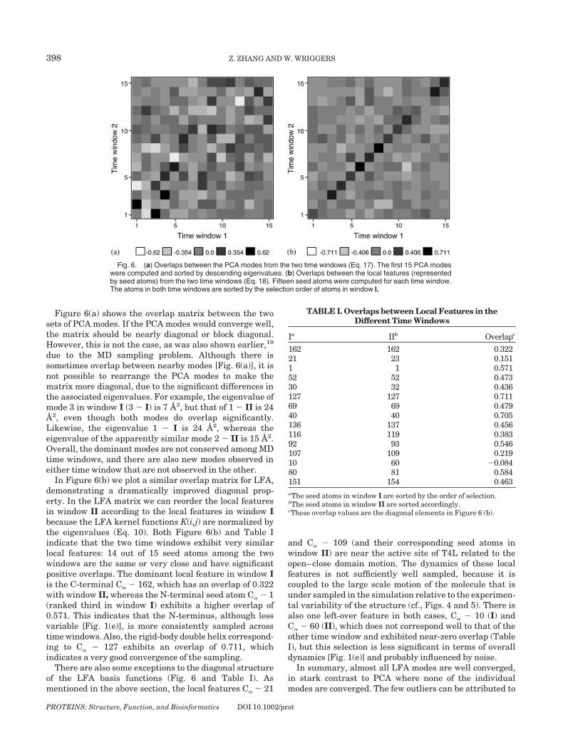
Figure 6(a) shows the overlap matrix between the twosets of PCA modes. If the PCA modes would converge well,the matrix should be nearly diagonal or block diagonal.However, this is not the case, as was also shown earlier,19

due to the MD sampling problem. Although there issometimes overlap between nearby modes [Fig. 6(a)], it isnot possible to rearrange the PCA modes to make thematrix more diagonal, due to the significant differences inthe associated eigenvalues. For example, the eigenvalue ofmode 3 in window I (3 � I) is 7 A2, but that of 1 � II is 24A2, even though both modes do overlap significantly.Likewise, the eigenvalue 1 � I is 24 A2, whereas theeigenvalue of the apparently similar mode 2 � II is 15 A2.Overall, the dominant modes are not conserved among MDtime windows, and there are also new modes observed ineither time window that are not observed in the other.

In Figure 6(b) we plot a similar overlap matrix for LFA,demonstrating a dramatically improved diagonal prop-erty. In the LFA matrix we can reorder the local featuresin window II according to the local features in window Ibecause the LFA kernel functions K(i,j) are normalized bythe eigenvalues (Eq. 10). Both Figure 6(b) and Table Iindicate that the two time windows exhibit very similarlocal features: 14 out of 15 seed atoms among the twowindows are the same or very close and have significantpositive overlaps. The dominant local feature in window Iis the C-terminal C� � 162, which has an overlap of 0.322with window II, whereas the N-terminal seed atom C� � 1(ranked third in window I) exhibits a higher overlap of0.571. This indicates that the N-terminus, although lessvariable [Fig. 1(e)], is more consistently sampled acrosstime windows. Also, the rigid-body double helix correspond-ing to C� � 127 exhibits an overlap of 0.711, whichindicates a very good convergence of the sampling.

There are also some exceptions to the diagonal structureof the LFA basis functions (Fig. 6 and Table I). Asmentioned in the above section, the local features C� � 21

and C� � 109 (and their corresponding seed atoms inwindow II) are near the active site of T4L related to theopen–close domain motion. The dynamics of these localfeatures is not sufficiently well sampled, because it iscoupled to the large scale motion of the molecule that isunder sampled in the simulation relative to the experimen-tal variability of the structure (cf., Figs. 4 and 5). There isalso one left-over feature in both cases, C� � 10 (I) andC� � 60 (II), which does not correspond well to that of theother time window and exhibited near-zero overlap (TableI), but this selection is less significant in terms of overalldynamics [Fig. 1(e)] and probably influenced by noise.

In summary, almost all LFA modes are well converged,in stark contrast to PCA where none of the individualmodes are converged. The few outliers can be attributed to

Fig. 6. (a) Overlaps between the PCA modes from the two time windows (Eq. 17). The first 15 PCA modeswere computed and sorted by descending eigenvalues. (b) Overlaps between the local features (representedby seed atoms) from the two time windows (Eq. 18). Fifteen seed atoms were computed for each time window.The atoms in both time windows are sorted by the selection order of atoms in window I.

TABLE I. Overlaps between Local Features in theDifferent Time Windows

Ia IIb Overlapc

162 162 0.32221 23 0.1511 1 0.57152 52 0.47330 32 0.436127 127 0.71169 69 0.47940 40 0.705136 137 0.456116 119 0.38392 93 0.546107 109 0.21910 60 �0.08480 81 0.584151 154 0.463aThe seed atoms in window I are sorted by the order of selection.bThe seed atoms in window II are sorted accordingly.cThese overlap values are the diagonal elements in Figure 6 (b).



under sampled global conformational changes that affectthe local dynamics, or to noise. We acknowledge that theentire subspace of the first 10 to 15 PCA modes is morerobust between time windows39 compared to the indi-vidual mode overlaps shown in Figure 6(a). In LFA, wetake advantage of this because the subspace of all localizedmodes is identical to the standard subspace of the PCAmodes used (Eq. 10). This is one of the reasons why most ofthe LFA modes are well converged even though individualPCA modes are not.

Relaxation Times

To illustrate the actual dynamics observed along indi-vidual modes, it is customary to project the MD trajectory

along the modes. In the above terminology, we are inter-ested in the outputs of both PCA and LFA representations.The PCA outputs Ar (Eq. 3) have length units and corre-spond to the deformation of a structure along a mode,whereas the LFA outputs O(i) (Eq. 6) are dimensionless,raising the question about their physical meaning. TheLFA outputs preserve all information of the PCA outputs,which are decorrelated and weighted by eigenvalue. �ArAq� r�rq. The factor 1/�r then normalizes the PCA outputsto unity, thus different Ar can be mixed by LFA (Eq. 8). Sothe LFA outputs {Oi}, which are decorrelated only in theasymptotic limit n 3 3N, give the contribution of eachDOF i to the protein dynamics in the low-dimensionalsubspace n �� 3N.

Fig. 7. Projections of the trajectory along the first three PCA modes (left) and their autocorrelation functions(right). (a) The first PCA mode, (b) the second PCA mode, and (c) the third PCA mode.



To compare the performance of PCA and LFA, we firstplotted the projections of the trajectory onto the threelargest eigenvalue PCA modes and calculated their autocor-relation functions (Fig. 7). The results show that theprojections along the low-frequency modes exhibit relax-ation times which are longer than the sampling timewindow, in agreement with Balsera and colleagues.19 Forthe dynamics to converge, the autocorrelation functionshould decay to 0 within the sampling time. This is notobserved because such global collective motions are undersampled by MD.

Figure 8 illustrates output functions of three local

features (C� � 109, C� � 52, and C� � 21) and theirautocorrelation functions. Although the first two LFAmodes have relaxed better than their global PCA counter-parts, the figure shows that the LFA modes still sufferfrom long relaxation times. Because the LFA outputsdepend on the low-frequency subspace from PCA, it cannot be expected that they solve the MD sampling problemsimply by virtue of a different statistical analysis. Forexample, there is a large fluctuation of the local featurecorresponding to C� � 109 in time window II (from about6.5 to 8.5 ns, which is also visible in Figure 4(b,c) (red).This rare event corresponding to a transient melting of an

Fig. 8. The output functions of local features (left), and their autocorrelation functions (right). The first 15PCA modes were used for LFA (n 15 in Eq. 8). Each local feature is represented by a seed atom, and theseed index selected by the sparsification algorithm: (a) x-component of C� � 109, (b) y-component of C� � 52,and (c) y-component of C� � 21.



�-helix prohibits short relaxation times of the correspond-ing output.

The most significant reduction in relaxation times canbe achieved by focusing on the intrinsic motions of theLFA domains. In Cartesian space, the results of PCAand LFA rely on what reference is used for fitting of thetrajectory frames. In the above, we least-squares fittedthe structures by all C� atoms, reflecting the globalscope of the PCA modes. However, the assignment oflocal dynamic domains enables us now to take advan-tage of the local reference frames of the LFA modes.After a P-weighted least-squared fitting, we recalcu-lated the local feature outputs from Equation 8. Theresults are shown in Figure 9. It can be noticed that the

decay of the autocorrelation is now clearly observed incontrast to the globally fitted PCA and LFA modes.Because we eliminated the interdomain motions (whichexhibit slower relaxation times), the remaining intrado-main relaxation times are of the order of 1 ns, whichenables the internal motion to be sampled within the 8ns simulation time frame.

CONCLUSIONS

This article represents the first application of LFA to thestudy of protein dynamics. The algorithm enables a segmen-tation of the system into local dynamic domains. In themodel system T4 lysozyme, these local features correspondto the most flexible parts in the protein, and they can be

Fig. 9. Same as Figure 8, except that we used a P-weighted least-squares fitting of the dynamic domains.In the weighting, negative values of the P matrix were set to 0.



related to functional domain motions. The overall func-tional motion can be well described by only a few of thelocal features.

LFA is a promising tool to study protein dynamics in areduced dimensional space. One of the major limitations ofthe traditional PCA-based statistics is the global support ofthe output basis functions. This effect is due to the forcedorthogonalization of the successive modes. In LFA, we con-struct a local topographic representation of objects in termsof local features from the global PCA modes. The majoradvantages of LFA are (1) the reproducibility of the modes[different sampling time windows exhibit nearly the samelocal features, see Figure 6(b) and Table I], and (2) the fastrelaxation times of intradomain motions when trajectoryframes are aligned by individual domains (Fig. 9).

Does LFA solve the MD sampling problem? As a statisti-cal tool LFA can be used for trajectory analysis but it doesnot by itself enhance sampling of rare or slow events thatare outside of the MD sampling window. However, themethod presents a robust way to isolate individual modesthat are under sampled, something that is not possiblewith PCA: Because most LFA modes are converged, onecan identify in the overlap matrix the small subset ofmodes that are affected by noise or by a coupling to anunder sampled large-scale motion in the biomolecule.

Do large proteins or macromolecular assemblies reallymove as statistically independent dynamic domains? Un-like PCA, the P-weighted LFA (Fig. 9) does not attempt toestimate a coherence of motion across large distances inbiomolecules. Because the sampling of such interdomaincoherence is out of reach for short MD simulations, anystatistical technique would risk to overestimate such acoherence in an under sampling situation. As a statisticalmodel the P-weighted LFA is focused mainly on thesampling of the well-converged intradomain motion andtherefore it is better adapted to the short MD dynamics.However, LFA does not rule out that long range interac-tions exist on much longer time scales.

How many local features are needed to describe thefunctional dynamics in the protein and how are thedynamic domains defined? We may chose the first n PCAmodes that contribute to a certain percentage of theoverall motion in the protein. In our system T4 lysozyme,the first 15 PCA modes out of 486 (about 3%) contribute tomore than 70% of the total fluctuation. Also, in thesparsification algorithm, we can keep adding seed atomsuntil the reconstruction error (Eq. 14) is below an accept-able value. In our case, the reconstruction error decreasesabout 60% after 5 seed atoms out of 15 are selected. Thesefive seed atoms are the C-terminal atom, C� � 109, C� �52, C� � 21, and the N-terminal atom, respectively [Fig.1(d)]. However, any n atoms can be used in principle toreconstruct the O(i) without error.

One possible improvement of the sparsification would bea simultaneous instead of a sequential optimization of theseed atoms involving a criterion that directly minimizesthe correlation between the dynamic domains. Currently,we define the boundary of a dynamic domain by thecontiguous atoms that have positive correlations with the

seed atom in terms of LFA theory. A threshold above thebackground noise level of the correlation may be analternative. These issues will be subject of future research.Overall, our initial work presented here demonstrates thatLFA shows much promise for many applications in predic-tion, sampling and classification of large-scale macromo-lecular structure and dynamics.

ACKNOWLEDGMENTS

We are grateful to Dr. Danny C. Sorensen at RiceUniversity for helpful discussions. Z. Z. was supported bythe Keck Center Pharmacoinformatics Training Programof the Gulf Coast Consortia.

REFERENCES

1. Karplus M. Molecular dynamics: applications to proteins. In: J.-L.Rivail, editor. Modelling of molecular structures and properties,volume 71, Studies in physical and theoretical chemistry. Amster-dam: Elsevier Science Publishers; 1990. p 427–461.

2. Brooks CL III, Karplus M, Pettitt BM. Proteins: A TheoreticalPerspective of Dynamics, Structure and Thermodynamics, volumeLXXI of Advances in Chemical Physics. New York: John Wiley &Sons, 1988.

3. Hernandez G, Jenney FE Jr., Adams MWW, LeMaster DM.Millisecond time scale conformational flexibility in a hyperthermo-phile protein at ambient temperature. Proc Natl Acad Sci U S A2000; 97:3166–3170.

4. Falke JJ. A moving story. Science 2002;295:1480–1481.5. Horiuchi T, Go N. Projection of Monte Carlo and molecular

dynamics trajectories onto the normal mode axes: human ly-sozyme. Proteins 1991;10:106–116.

6. Kitao A, Hirata F, Go N. The effects of solvent on the conformationand the collective motions of proteins: normal mode analysis andmolecular dynamics simulations of Melittin in water and invacuum. Chem Phys 1991;158:447–472.

7. Amadei A, Linnsen ABM, Berendsen HJC. Essential dynamics ofproteins. Protein 1993;17:412–425.

8. van Aalten MF, Amadei A, Linssen ABM, Eijsink VGH, Vriend G,Berendsen HJC. The essential dynamics of Thermolysin: conforma-tion of the hinge-bending motion and comparison of simulations invacuum and water. Proteins 1995;22:45–54.

9. Garcıa AE. Large-amplitude nonlinear motions in proteins. PhysRev Lett 1992;68:2696–2699.

10. Kitao A, Go N. Investigating protein dynamics in collectivecoordinate space. Curr Opinion Struct Biol 1999;9:164–169.

11. Berendsen HJC, Hayward S. Collective protein dynamics inrelation to function. Curr Opinion Struct Biol 2000;10:165–169.

12. Brooks BR, Janezic D, and Karplus M. Harmonic analysis of largesystems I. Methodology. J Comput Chem 1995;16:1522–1542.

13. Case DA. Normal mode analysis of protein dynamics. CurrOpinion Struct Biol 1994;4:285–290.

14. Karhunen K. Uber lineare Methoden in der Wahrscheinlichkeitsre-chnung. Ann Acad Sci Fennicae Ser. A137, 1947.

15. Karplus M, Jushick JN. Method for estimating the configurationalentropy of macro-molecules. Macromolecules 1981;14:325–332.

16. Levy RM, Srinivasan AR, Olson WK, McCammon JA. Quasihar-monic method for studying very low frequency modes in proteins.Biopolymers 1984;23:1099–1112.

17. Kitao A, Hayward S, Go N. Energy landscape of a native protein:jumping-among-minima model. Proteins 1998;33:496–517.

18. Clarage JB, Romo T, Andrews BK, Pettitt BM, Phillips GN. Asampling problem in molecular dynamics simulations of macromol-ecules. Proc Natl Acad Sci U S A 1995;92:3288–3292.

19. Balsera MA, Wriggers W, Oono Y, Schulten K. Principal compo-nent analysis and long time protein dynamics. J Phys Chem1996;100(7):2567–2572.

20. Tama F, Sanejouand Y.-H. Conformational change of proteinsarising from normal mode calculations. Protein Eng 2001;14:1–6.

21. Lee DD, Seung HS. Learning the parts of objects by non-negativematrix factorization. Nature 1999;401:788–791.

22. Paatero P. Least squares formulation of robust non-negativefactor analysis. Chemometrics Intell Lab Sys 1997;37:23–35.



23. Penev PS, Atick JJ. Local feature analysis: a general statisticaltheory for object representation. Network: Computation in NeuralSystems 1996;7:477–500.

24. Janezic D, Venable RM, Karplus M. Harmonic analysis of largesystems III. Comparison with molecular dynamics. J. Comp Chem1995;16:1554–1568.

25. Li Z, Atick J. Towards a theory of the striate cortex. Neural Comp1994;6:127–146.

26. Berendsen HJC, van der Spoel D, van Drunen R. Gromacs: Amessage-passing parallel molecular dynamics implementation.Comput Phys Commun 1995;91:43–56.

27. Lindahl E, Hess B, van der Spoel D. Gromacs 3.0: A package formolecular simulation and trajectory analysis. J Mol Model 2001;7:306–317.

28. Anderson WF, Grutter MG, Remington SJ, Weaver LH, MatthewsBW. Crystallographic determination of the mode of binding ofoligosaccharides to T4 bacteriophage lysozyme: implications forthe mechanism of catalysis. J Mol Biol 1981;147:523–543.

29. Faber HR, Matthews BW. A mutant T4 lysozyme displays fivedifferent crystal conformations. Nature 1990;348:263–266.

30. Zhang XJ, Wozniak JA, Matthews BW. Protein flexibility andadaptability seen in 25 crystal forms of T4 lysozyme. J Mol Biol1995;250:527–552.

31. Weaver LH, Matthews BW. Structure of bacteriophage T4 ly-sozyme refined at 1.7 A resolution. J Mol Biol 1987;193:189–199.

32. Berendsen HJC, Postma JPM, van Gunsteren WF, Hermans J.Interaction models for water in relation to protein hydration. In:B. Pullman, editor. Intermolecular forces. Dordrecht, Nether-lands; Reidel 1981. p. 331–342.

33. Berendsen HJC, Postma JPM, van Gunsteren WF, DiNola A,Haak JR, Molecular dynamics with coupling to an external bath.J Chem Phys, 1984;81(8):3684–3690.

34. Hess B, Bekker H, Berendsen HJC, Fraaije GJEM. A linearconstraint solver for molecular simulations. J Comput Chem1997;18:1463–1472.

35. Essman U, Perela L, Berkowitz ML, Darden T, Lee H, PedersenLG. A smooth particle mesh ewald method. J Chem Phys 1995;103:8577–8592.

36. Humphrey WF, Dalke A, Schulten K. VMD - Visual MolecularDynamics. J Mol Graphics 1996;14:33–38.

37. de Groot BL, Hayward S, van Aalten DMF, Amadei A, BerendsenHJC. Domain motions in bacteriophage T4 lysozyme: a compari-son between molecular dynamics and crystallographic data. Pro-teins 1998;31:116–127.

38. Zhang Z, Shi Y, Liu H. Molecular dynamics simulations ofpeptides and proteins with amplified collective motions. Biophys J2003;84:3583–3593.

39. Amadei A, de Groot BL, Ceruso MA, Di Nola A, Berendsen HJC. Akinetic model for the internal motions of proteins: diffusionbetween multiple harmonic wells. Proteins 1999;35:283–292.



Local Feature Analysis: A Statistical Theory for Reproducible

Documents

Transcript of Local Feature Analysis: A Statistical Theory for Reproducible