Robust Regression for Minimum-Delay Load-Balancing F. Larroca and J.-L. Rougier

Load Balancing in Delay-LimitedDistributed Systems
by
Sagar Dhakal
B.E. Electrical and Electronics Engineering,
Birla Institute of Technology, May 2001
THESIS
Submitted in Partial Fulfillment of the
Requirements for the Degree of
Master of Science
Electrical Engineering
The University of New Mexico
Albuquerque, New Mexico
December, 2003

c©2003, Sagar Dhakal
iii

Dedication
To my dearest parents
iv

Acknowledgments
I would like to express sincere gratitude towards my advisor, Professor Majeed M.
Hayat, for his guidance, encouragement and support throughout this thesis work.1
His enthusiasm in research and teaching has been a perennial source of inspiration
to me. Working with him provided me an excellent learning opportunity.
I would like to thank Professor Chaouki T. Abdallah for sharing his expertise in
the field of time-delay systems and for motivating me. I would also like to thank my
other thesis committee member, Professor Gregory L. Heileman, for his support and
helpful comments.
I take this opportunity to thank my colleagues, Jean Ghanem and Biliana
Paskaleva, for their help and contribution to the successful completion of this work.
My heartfelt gratitude to all those who in some way helped me achieve my objective.
Finally, I thank my family for their immense love, patience and support.
1This work was supported by the National Science Foundation under Information Tech-
nology Research (ITR) grant No. ANI-0312611.
v
Load Balancing in Delay-LimitedDistributed Systems
by
Sagar Dhakal
ABSTRACT OF THESIS
Submitted in Partial Fulfillment of the
Requirements for the Degree of
Master of Science
Electrical Engineering
The University of New Mexico
Albuquerque, New Mexico
December, 2003
Load Balancing in Delay-LimitedDistributed Systems
by
Sagar Dhakal
B.E. Electrical and Electronics Engineering,
Birla Institute of Technology, May 2001
M.S., Electrical Engineering, University of New Mexico, 2003
Abstract
Load balancing is the allocation of the workload among a set of co-operating compu-
tational elements (CEs). In large-scale distributed computing systems, in which the
CEs are physically or virtually distant from each other, there are communication-
related delays that can significantly alter the expected performance of the load-
balancing policies that do not account for such delays. This is a particularly promi-
nent problem in systems for which the individual units are connected by means of
a shared broadband communication medium (e.g., the Internet, ATM, ad hoc net-
works, wireless LANs or the wireless Internet). In such cases, the delays, in addition
to being large, fluctuate randomly, making their one-time accurate prediction im-
possible. Therefore, the performance of such distributed systems under any load
balancing policy is stochastic in nature and must be assessed in a statistical sense.
Moreover, the design of load-balancing policies that best suits such delay-infested
distributed systems must also be carried out in a statistical framework.
vii

In this work we study the effect of random delays (small and large) on the perfor-
mance of a dynamic load-balancing algorithm. The study shows that the presence
of random delay leads to a significant degradation in the performance of a load-
balancing policy. Therefore, we exploit the stochastic dynamics, using a queuing
framework, to model the load-balancing algorithm and optimize its performance.
We find that weakening the load-balancing mechanism, or so-called gain, appropri-
ately leads to an improved performance of the distributed system. Motivated by
this fact, we consider the optimization problem for a policy that has a fixed (one
or two) number of balancing instants while optimizing the policy over the strength
of load balancing and the times when the schedulings are executed. We discuss the
performance of a single-scheduling policy on a distributed physical system consisting
of a wireless LAN.
To look into the interplay between delay and load-balancing gain, we develop a
novel analytical model to characterize the mean of the total completion time for a
distributed system when a single scheduling is performed. We then use our optimal
single-time load-balancing strategy to propose an autonomous on-demand (sender
initiated) load-balancing scheme.
viii

Contents
1 Introduction 1
1.1 Problem Description and Motivation . . . . . . . . . . . . . . . . . . 1
1.2 General Framework for Load Balancing . . . . . . . . . . . . . . . . . 3
1.3 Objective of this Thesis . . . . . . . . . . . . . . . . . . . . . . . . . 5
1.4 Overview of Thesis . . . . . . . . . . . . . . . . . . . . . . . . . . . . 6
2 Taxonomy of Load Balancing Policies 8
2.1 Brief Overview of Balancing Policies . . . . . . . . . . . . . . . . . . 8
2.1.1 Static versus Dynamic Load Balancing . . . . . . . . . . . . . 8
2.1.2 Local versus Global Load Balancing . . . . . . . . . . . . . . . 9
2.1.3 Centralized versus Distributed Load Balancing . . . . . . . . . 10
2.1.4 Sender/Receiver/Symmetrically Initiated Balancing . . . . . . 11
2.1.5 Deterministic versus Non-deterministic Load Balancing . . . . 11
2.2 Related Work . . . . . . . . . . . . . . . . . . . . . . . . . . . . . . . 11
ix

Contents
2.2.1 Graph Partitioning Method . . . . . . . . . . . . . . . . . . . 12
2.2.2 Balancing scheme for SAMR Applications . . . . . . . . . . . 13
2.2.3 Hydrodynamic Algorithm . . . . . . . . . . . . . . . . . . . . 15
2.2.4 Gang-scheduling, Backfilling, and Migration . . . . . . . . . . 17
2.2.5 Load Balancing using Queuing Theory . . . . . . . . . . . . . 19
3 Dynamic Load Balancing: A Stochastic Approach 21
3.1 Load Balancing in Deterministic Delay Systems . . . . . . . . . . . . 22
3.2 Description of the Stochastic Dynamics . . . . . . . . . . . . . . . . . 24
3.3 A Discrete-time Queuing Model with Delays . . . . . . . . . . . . . . 25
3.4 Simulation Results . . . . . . . . . . . . . . . . . . . . . . . . . . . . 27
3.4.1 Effect of Delay . . . . . . . . . . . . . . . . . . . . . . . . . . 29
3.4.2 Interplay Between Delay and the Gain Coefficient K . . . . . 31
3.4.3 Load Dependent Delay . . . . . . . . . . . . . . . . . . . . . . 32
3.5 Summary and Conclusions . . . . . . . . . . . . . . . . . . . . . . . . 36
4 Discrete-Time Load Balancing 38
4.1 Motivation . . . . . . . . . . . . . . . . . . . . . . . . . . . . . . . . . 39
4.2 Simulation Results . . . . . . . . . . . . . . . . . . . . . . . . . . . . 40
4.2.1 Single Load-balancing Strategy . . . . . . . . . . . . . . . . . 41
4.2.2 Double Load-balancing Strategy . . . . . . . . . . . . . . . . . 46
x

Contents
4.3 Experimental Results . . . . . . . . . . . . . . . . . . . . . . . . . . . 50
4.3.1 Description of the experiments . . . . . . . . . . . . . . . . . . 50
4.3.2 Discussion of results . . . . . . . . . . . . . . . . . . . . . . . 51
4.4 Simulation Results . . . . . . . . . . . . . . . . . . . . . . . . . . . . 54
4.5 Conclusions . . . . . . . . . . . . . . . . . . . . . . . . . . . . . . . . 55
5 Stochastic Analysis of the Queuing Model: A Regeneration Ap-
proach 58
5.1 Rationale . . . . . . . . . . . . . . . . . . . . . . . . . . . . . . . . . 59
5.2 Dynamic Model Base . . . . . . . . . . . . . . . . . . . . . . . . . . . 60
5.3 Solving Eqn. (5.9) . . . . . . . . . . . . . . . . . . . . . . . . . . . . . 64
5.3.1 Description . . . . . . . . . . . . . . . . . . . . . . . . . . . . 64
5.3.2 Initial Condition . . . . . . . . . . . . . . . . . . . . . . . . . 67
5.4 Summary of the Steps for Calculating µ1,1m,n(tb) . . . . . . . . . . . . . 72
6 Future Work: On-Demand Sender-Initiated Dynamic Load Balanc-
ing 73
Appendices 76
A Monte Carlo Simulation Software Developed in MATLAB 77
B MATLAB Code for Solving Equations Iteratively 94
xi

Contents
References 98
xii

Chapter 1
Introduction
1.1 Problem Description and Motivation
The demand for high performance computing continues to increase everyday. The
computational need in areas like cosmology, molecular biology, nanomaterials, etc.,
cannot be met even by a small group of fastest computers available [16, 17, 18, 19].
But with the availability of high speed networks, a large number of geographically dis-
tributed computational elements (CEs) can be interconnected and effectively utilized
in order to achieve a performance which is not ordinarily attainable on a single CE.
The distributed nature of this type of computing environment calls for consideration
of heterogeneities in computational and communication resources. A common archi-
tecture is the cluster of otherwise independent CEs communicating through a shared
network. Incoming workload has to be efficiently allocated to these CEs so that no
single CE is overburdened where one or more other CEs remain idle. Further, tasks
migration from high to low traffic area in a network alleviates the network-traffic
congestion problem up to some extent.
Distributing the total computational load across available processors is referred
1

Chapter 1. Introduction
to as load balancing in the literature. Effective load balancing of a cluster of CEs
in a distributed computing system relies on accurate knowledge of the state of the
individual CEs. This knowledge is used to judiciously assign incoming computational
tasks to appropriate CEs, according to some load-balancing policy [1, 23]. In large-
scale distributed computing systems in which the CEs are physically or virtually
distant from each other, there are a number of inherent time-delay factors that can
seriously alter the expected performance of the load-balancing policies that do not
account for such delays. One manifestation of such time delay is attributable to
the computational limitations of individual CEs. A more significant manifestation
of such delay arises from the communication limitations between the CEs. These
include delays in transferring loads between CEs and delays in the communication
between them. Moreover, these delay elements not only fluctuate within each CE,
as the amounts of the loads to be transferred vary, but also vary as a result of
the uncertainty in the condition of the communication medium that connects the
units. This kind of delay-uncertainty is frequently observed in systems for which
the individual units are connected by means of a shared broadband communication
medium (e.g., the Internet, ATM, ad hoc networks, wireless LANs or the wireless
Internet).
There has been extensive research in the development of the appropriate dynamic
load balancing policies (some of which will be discussed in Chapter 2 of this thesis).
Some of these existing approaches consider constant performance of the network while
others consider deterministic communication and transfer delay. The load balancing
schemes designed under this conviction undermine the randomness in delay. But it
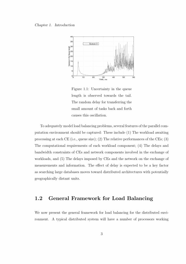
is observed through Fig1.1 that this randomness in delay leads to an unnecessary
exchange of tasks between CEs which results in an oscillatory behavior of the queues.
In this thesis, we will propose and investigate a dynamic load balancing scheme for
distributed systems which incorporates the stochastic nature of the delay in both
communication and load transfer.
2
Chapter 1. Introduction
0 10 20 30 40 50 600
5
10
15
20
25
30
35
40
TIME, ms
Varia
nce
in th
e Q
ueue
leng
th
Queue 3
Figure 1.1: Uncertainty in the queue
length is observed towards the tail.
The random delay for transferring the
small amount of tasks back and forth
causes this oscillation.
To adequately model load balancing problems, several features of the parallel com-
putation environment should be captured: These include (1) The workload awaiting
processing at each CE (i.e., queue size); (2) The relative performances of the CEs; (3)
The computational requirements of each workload component; (4) The delays and
bandwidth constraints of CEs and network components involved in the exchange of
workloads, and (5) The delays imposed by CEs and the network on the exchange of
measurements and information. The effect of delay is expected to be a key factor
as searching large databases moves toward distributed architectures with potentially
geographically distant units.
1.2 General Framework for Load Balancing
We now present the general framework for load balancing for the distributed envi-
ronment. A typical distributed system will have a number of processors working
3
Chapter 1. Introduction
independently with each other. Some of them are linked by communication channel
and while some are not. Each processor possesses an initial load, which represents
an amount of work to be performed, and each may have a different processing ca-
pacity. To minimize the time needed to perform all tasks, the workload has to be
evenly distributed over all processors based on their processing speed. This is why
load balancing is needed. If all communication links are of infinite bandwidth and
instantaneous, the load distribution would suffer from no delay, and this does not
represent the distributed environments considered in this thesis. But in any practi-
cal distributed systems, the channels are of finite bandwidth and and the units may
be physically distant; therefore, we would encounter information-flow bottlenecks.
Obviously, we do not want to send packets in a noisy channel with sufficiently large
delays and prone to packet loss. Therefore, load balancing is also a decision making
process of whether to allow tasks migration or not. The situation is aggravated by
the fact that the delay involved is random in nature.
Another issue related to load balancing is that a job is not arbitrarily divisible
leading to certain constraints in dividing tasks. Each job consists of several smaller
tasks and each of those tasks can have different execution time. Also, the load on
each processor as well as on the network can vary from time to time based on the
workload brought about by the users. The processor capacity may be different from
each other in architecture, operation system, CPU speed, memory size, and available
disk space. The load balancing problem also needs to consider fault-tolerance and
fault-recovery. With all these factors taken into account, load balancing can be
generalized into four basic steps: (1) Monitoring processor load, (2) Exchanging load
information between processors , (3) Calculating the new work distribution, and (4)
Actual data movement. Numerous load balancing schemes have been proposed and
implemented and we will look into some of them in Chapter 2. Broadly speaking,
the goal of a load balancing algorithm is to redistribute the load to minimize the
overall execution time. Clearly, the search has to be directed to find the algorithm
4

Chapter 1. Introduction
which gives an optimal solution. However, most of the available literature in load
balancing consider the problem as NP-complete and attempts solving the problem
heuristically or suboptimally.
1.3 Objective of this Thesis
The main goal of this thesis is to investigate the effect of stochastic delay on the
performance of a load balancing policy in a distributed environment and find a
remedy to upgrade the performance. The purpose is oriented to come up with a
better decision making policy to tackle the randomness in delay. This thesis work
does not address issues like divisibility of a job, network architecture, operating
system, memory size, fault-tolerance and fault-recovery. In the existing literature
[13, 14, 15, 2, 20, 21, 25, 23, 24], the balancing policies have been developed where
delay has been considered as deterministic and predictable. However, our view is
this kind of policy will not perform as expected in real situations where network is
shared (as described earlier in Section 1.1), channels have high bit-error rates and
the level of traffic fluctuates every now and then. This uncertainty in delay will have
a further destabilizing effect. Therefore, there is a need to come up with an improved
balancing policy which takes into account the random nature of the delay.
For a given workload distribution among a group of heterogeneous processors,
we recognize the overall completion time of the group as the performance metric,
and the objective is to develop a balancing strategy which minimizes this. First, we
identify the feasibility of this kind of optimization by undertaking a Monte-Carlo
(MC) simulation approach. We then verify the validity of the assumptions used in
the MC approach and further apply our load-balancing scheme to a physical system
consisting of a wireless LAN. We then launch a novel, analytical stochastic approach,
based on renewal principles, that characterizes the average completion time. We
5

Chapter 1. Introduction
present the results for the case of two nodes (n = 2); however, the approach can be
extended to the multi-CE case in a straightforward fashion. Notably, the n = 2 case
maintains the gist of the multi-CE problem and conveys the underlying principles of
our analytical solution while keeping the algebra at a minimum. Therefore, our aim is
to analytically model this 2-processor system and define a way to apply the model for
dynamic load balancing. This thesis work may also have the potential for being useful
in other fields such as networked control systems (NCS) and teleautonomy. In a NCS
the sensor and the controller are connected over a shared network and therefore, there
is a delay in closing the feedback loop. A special application of teleautonomy [35, 36]
is: robots distributed geographically and working autonomously but at the same time
being monitored by a distant controller. Clearly, the randomness in communication
delay degrades the performance of such systems.
1.4 Overview of Thesis
In Chapter 2, we present an overview of existing balancing strategies. We start by
briefly discussing different schemes. We then look into special types of load balancing
schemes available in the literature. Chapter 3 begins with the brief introduction to
load balancing scheme developed by the authors of [23, 24, 25, 26] for modelling deter-
ministic time-delay systems. We utilize some features from this model to develop our
balancing strategy. Next, we present a discrete-time stochastic dynamical-equation
model describing the evolution of the random queue size of each node. We generate
a MC simulation algorithm and use it to demonstrate the extent of the role played
by the magnitude and uncertainty of the various time-delay elements in altering the
performance of load balancing. Chapter 4 presents the drawback in the implemen-
tation of a load balancing policy on a continuous basis in a delay-limited distributed
computing environment. We present the single and the double load balancing strate-
6

Chapter 1. Introduction
gies. The performance of the single load balancing strategy on a distributed physical
system is discussed and is compared to our simulation results. Based on the concept
of regeneration, in Chapter 5 we present a mathematical model for the distributed
system with two nodes where one-shot balancing is done. We obtain a system of
four difference-differential equations characterizing the mean of the overall comple-
tion time. Finally, in Chapter 6 we propose a dynamic load balancing scheme which
utilizes the analytical model developed in Chapter 5.
7

Chapter 2
Taxonomy of Load Balancing
Policies
There has been an extensive research in the development of the appropriate load
balancing policy. The policies can broadly be categorized as static, dynamic, local,
global, centralized, distributed, sender-initiated, receiver initiated, symmetrically-
initiated, deterministic and non-deterministic.
2.1 Brief Overview of Balancing Policies
2.1.1 Static versus Dynamic Load Balancing
Static load distribution assigns jobs to nodes probabilistically or deterministically,
without consideration of runtime events. For example, using a simple static strategy,
tasks can be assigned to processors in a round-robin fashion so that each processor
executes approximately the same number of tasks. This approach works better when
the workload can be accurately characterized and the system dynamics do not fluc-
8

Chapter 2. Taxonomy of Load Balancing Policies
tuate. The runtime overhead involved is very small since processors know exactly
which tasks they are to execute based on their processor numbers and the task iden-
tifiers. It is generally impossible to predict or collect task characteristics like arrival
time, execution costs, interdependencies, etc., and therefore, static balancing scheme
has a very limited application.
Dynamic load distribution is designed to overcome the problems of unknown or
uncharacterizable workloads and the non-deterministic run-time performance vari-
ation of the nodes. In this unpredictable environment, it is better to perform the
load balancing more than once or periodically during run-time such that the prob-
lem’s variable behavior more closely matches available computational resources. For
example, in areas like molecular dynamics, fluid dynamics, etc., the computational
requirement associated with different parts of a problem domain may change with
time as the computation progresses. In dynamic scheduling, the overhead associ-
ated with the task of scheduling can directly affect the performance of the systems.
Therefore, it is vital to look into issues related to where and when scheduling is per-
formed, where the information required for scheduling is stored, and how complex
the scheduling algorithm can be. In this thesis, we focus on the dynamic balancing
domain.
2.1.2 Local versus Global Load Balancing
In a local load balancing scheme, each processor polls other processors in its small
neighborhood and uses this local information to decide upon a load transfer. At
every step a processor communicates with its nearest neighbors in order to achieve a
local balance. The primary objective is to minimize remote communication as well
as to efficiently balance the load on the processors. However, in a global balancing
scheme, a certain amount of global information is used to initiate the load balancing.
9

Chapter 2. Taxonomy of Load Balancing Policies
The DASUD (Diffusion Algorithm Searching Unbalanced Domains) [3] algorithm
belongs to the nearest neighbors classes. The authors evaluate the performance of
the DASUD algorithm across ring, torus and hypercube topologies and observe via
simulations that this balancing scheme outperforms the strategies for global balance
degree in these cases. In [2], the authors divide the load balancing process into
global load balancing phase and local load balancing phase so as to capture the
heterogeneity of the network. The redistribution cost and the computational gain
has to be compared before invoking any global distribution.
2.1.3 Centralized versus Distributed Load Balancing
Centralized schemes [4, 5] store global information at a centralized location and use
this information to make more comprehensive scheduling decisions using the com-
puting and storage resources of one or more dedicated processors. In some strategies,
the sending or receiving processors contact a specific scheduling processor to identify
another processor to which tasks are sent or from which tasks are received. There
is always a contention to access the shared information and request tasks for execu-
tion, which may cause the designated processor to become bottleneck. Further, the
scheme fails if the designated processor crashes.
In distributed scheduling [25, 23, 26, 24, 6, 7, 8, 1], the scheduling task and the
scheduling information are distributed among the processors and their memories. In
some cases [6, 7, 8], the scheme allows idle processor to assign tasks to themselves at
runtime by accessing a shared global queue. The time required to access this shared
queue to remove one or more tasks from the common pool of waiting tasks might
introduce runtime overhead.
10

Chapter 2. Taxonomy of Load Balancing Policies
2.1.4 Sender/Receiver/Symmetrically Initiated Balancing
Techniques of scheduling tasks in distributed systems have been divided mainly as
sender-initiated, receiver-initiated, and symmetrically-initiated. In sender-initiated
algorithms [9, 10, 1, 23, 26], the overloaded nodes transfer one or more of their tasks
to more under-loaded nodes. In receiver-initiated schemes [4, 11, 10], under-loaded
nodes request tasks to be sent to them from nodes with higher loads. In symmetric
approach [10, 12], both the under-loaded as well as the loaded nodes can initiate load
transfers.
2.1.5 Deterministic versus Non-deterministic Load Balanc-
ing
In deterministic load balancing, the information about tasks to be scheduled and
their relation to one another is entirely known prior to their execution time. In
non-deterministic some information may not be known prior to execution. Both
deterministic and non-deterministic scheduling can be implemented using all the
above discussed balancing methodologies.
2.2 Related Work
In this section we present some load balancing models and approaches available in
the literature [13, 14, 15, 2, 20, 21].
11

Chapter 2. Taxonomy of Load Balancing Policies
2.2.1 Graph Partitioning Method
In [13], the authors presents a heuristic method for partitioning arbitrary graphs and
show that it is both effective in finding optimal partitions, and fast enough to be
practical in solving large problems like load balancing in distributed environment.
We give a brief exposition to the method used by the authors to partition the graph.
The authors consider a graph G of n nodes with cost on its edges and the objective
is to partition the nodes into subsets of given sizes so as to minimize the sum of
the costs on all edge cuts. The nodes are assigned sizes(weights) wi, i = 1, ..., n
such that for all i, 0 < wi ≤ p for some p > 0. They define a connectivity matrix
C = (cij), i, j = 1, ..., n which describe the edges of G. Now, for any k ∈ N , a
k −way partition of G is a set of nonempty, pairwise disjoint subsets of G, given by
v1, ..., vk such that⋃k
i=1 vi = G. The k −way partition is allowed if |vi| ≤ p for all i,
where the symbol |vi| =∑
wi. Finally, the cost of a partition is the summation of
cij over all possible i and j such that i and j are in different subsets, i.e. the cost
is the sum of all external costs in the partition. The performance metric is thus to
find a minimal-cost admissible partition of G.
The authors show that finding an optimal solution using a strictly exhaustive
procedure requires an inordinate amount of computation, and therefore, solving the
problem heuristically is a quick approach to produce good solutions. First, they find
the minimal-cost partition of a given graph into two-subsets (k = 2). They start
with 2n points in the original graph and partition it arbitrarily into two sets A and
B, each with n points. The goal here is to try to decrease the initial cost T by a
series of interchanges of subsets of A and B. Every time an interchange is made,
the cumulative gain associated with it and with all prior interchanges is calculated
according to their algorithm. Finally, when there is no more room for the reduction in
initial cost, the partition is called locally optimum partition. Now, the local optimum
partition is perturbed so that an iteration of the process on the perturbed solution
12

Chapter 2. Taxonomy of Load Balancing Policies
will yield a further reduction in the total cost. If it leads to an improvement, the new
solution thus obtained is considered to be the optimal partition. The authors call it
a global optimal solution. Now, the authors relax the requirement for the nodes of
the graph to be of the same size. They achieve this by converting any node of size
s > 1 to a cluster of s nodes of size 1, bound together by edges of appropriately high
cost. Finally, the idea of 2-way partition is extended to perform k-way partition.
They start with any arbitrary k sets each with n nodes and by repeated application
of the 2-way partitioning procedure to pair of subsets, they make the partition as
close as possible to being pairwise optimal. The authors say that this may not lead
to a globally optimal k-way partition, there may be situations where interchanges
involving three or more items from three or more subsets is required. Also, the
choice of the starting partitions will determine how fast the solution converges to
being pairwise optimal. This concept is utilized in load balancing by modelling the
cost on the nodes as the number of tasks and the edge cost as the amount of data
transfer between the nodes. Partitioning is done to make the cost on each processing
node equal while minimizing the respective edge costs. This model takes into account
the computation and the communication costs but considers them deterministic.
2.2.2 Balancing scheme for SAMR Applications
In [2] the authors propose a dynamic load balancing algorithm for Structured Adap-
tive Mesh Refinement (SAMR) applications on distributed systems. The focus is on
the heterogeneity and dynamic load of the networks which are essentially prevalent
in a distributed regime. SAMR is an algorithm used in multidimensional numerical
simulations to achieve high resolution in localized regions and the authors mention
that the algorithm has already been applied to model computational fluid dynamics,
computational astrophysics, meteorological simulations, structural dynamics, mag-
netic, and thermal dynamics. ENZO is a parallel implementation of this algorithm
13

Chapter 2. Taxonomy of Load Balancing Policies
for astrophysical and cosmological applications. Obviously, SAMR requires a large
amount of computation, and therefore, the authors have appropriately chosen to ex-
ecute SAMR applications on distributed systems by dynamically assigning the work-
load among the systems at runtime. The authors execute ENZO on a distributed
system (WAN), and compare the performance with its parallel implementation. The
load balancing scheme is designed to reduce the overhead introduced by the WAN
in the distributed system. The available processors are divided into groups: a group
is defined as a homogeneous system and all the processors assigned to it have the
same performance and share an intra-connected network. The load balancing within
a group is referred as a local load balancing and the balancing among the groups
as global balancing. The authors define their distributed systems to contain two
or more groups. The objective is to minimize remote communication as well as to
efficiently balance the load on the processors.
The balancing scheme is divided into two phases: 1. Global load balancing phase
and 2. Local load balancing phase. The global balancing phase occurs after each
time-step but only at level 0 of SAMR algorithm. The evaluation of workload redistri-
bution cost among groups is made and this includes communication and computation
overhead. The authors heuristically come up with an expression for redistribution
cost which is: Cost = (α + β × W ) + δ, where α is the communication latency,
β is the communication transfer rate, W is the amount of workload in bytes to be
redistributed and δ is the computational overhead calculated using past information.
Similarly, the estimated computational gain for global load balancing at that par-
ticular time is also evaluated. For each group, the total workload (including all the
levels) is calculated for one time-step at level 0 using the past data and then the dif-
ference of total workload between groups is estimated. Finally, computational gain
is estimated by using the difference of total workload and the recorded execution
time of one iteration at the top level. Now, the global load balancing is invoked only
if the computational gain is some factor times the redistribution cost. The factor is
14

Chapter 2. Taxonomy of Load Balancing Policies
a user-defined parameter to control the strength of global load balancing. While re-
distribution among the groups, the authors come up with simple scheme to consider
the heterogeneity of processors. Each processor has a performance weight, and the
workload assigned to a group is weighted by the ratio of sum of performance weights
of the processors belonging to this group to the sum of the performance weights
of the entire processors in the system. Within each time-step for global balancing,
balancing is performed at the local level number of times. The local balancing is
done within a group and hence remote communication is avoided. ENZO is invoked
whenever a local balancing is performed at the local level. Therefore, the dynamic
load balancing proposed by the authors apply distributed scheme at the global level
and ENZO at the local level. The experiments performed by the authors according
to this scheme show that the total execution time can be reduced by 9% to 46% and
get an improvement of 26% over the case where only ENZO is applied to the whole
distributed system. We think that the performance of this policy can be further im-
proved if we have a clear picture of how the stochastic delay affects the redistribution
cost in the global balancing step, which the authors do not look at.
2.2.3 Hydrodynamic Algorithm
In the approach given in [14], each processor is viewed as a liquid cylinder where
the cross-sectional area corresponds to the capacity of the processor, the commu-
nication links are modelled as liquid channels between the cylinders, the workload
is represented by liquid, and the load balancing algorithm manages the flow of the
liquid. The objective is to reach the state where the heights of the liquid columns are
the same in all the cylinders. The computing system is modelled as an undirected
graph G = (N,E) where N is the set of processors and E represents the network
topology. The authors propose a general hydrodynamic framework to redistribute
the workload among the processors such that each processor obtains its share of the
15

Chapter 2. Taxonomy of Load Balancing Policies
workload proportional to its capacity. They define a potential energy function for
G such that its minimum value corresponds to the state of equilibrium where the
heights of the liquid columns are the same in all the cylinders. The nearest-neighbor
approach is used to migrate tasks among the processors.
Each processor ni has its processing capacity ci > 0 and load li which it is
currently running. Further, each ni is associated with a liquid cylinder whose cross-
sectional corresponds to ci. ∀ni ∈ N the potential energy of the liquid column in ni
is defined as PE(ni) =cih
2
i
2, where hi is the height of the liquid column in ni. Now,
the global potential energy of G is defined as the sum of potential energies of all the
nodes. The authors consider an infinitely thin liquid channel joining the bottom of
two liquid cylinders if there is a connection between the two corresponding processors.
The global fairness is said to be achieved when the heights of the liquid columns in
the cylinders are equal. They show that this state of equilibrium corresponds to the
minimum global potential energy. The amount of workload that is transferred from
node ni to node nj is given by γcicj
ci+cj(hi − hj) where γ is defined as the balancing
factor which is in the range (0, 1) and is used to control the amount of workload
flow. It is assumed that the communication channels have fixed delay times such
that load balancing activity is completed within a finite interval B. Every load
balancing step has two phases: information exchange and migration. The authors
show that with this approach, the global potential energy converges geometrically to
the optimal state. They applied the balancing scheme on eight network topologies:
binary tree, complete, hypercube, linear, mesh, ring, star and torus, and found that
the hypercube and torus generate the lowest load balancing time. The authors have
not addressed the issue of stochastic delay in this work.
16

Chapter 2. Taxonomy of Load Balancing Policies
2.2.4 Gang-scheduling, Backfilling, and Migration
The authors of [15] discuss three techniques: backfilling, gang-scheduling and migra-
tion to improve response times, throughput and utilization in large super computing
environments. Backfilling is a purely space-sharing approach while gang-scheduling
is time-sharing strategy and migration corresponds to moving a job from one virtual
machine to the other.
Backfilling attempts to assign unutilized nodes to jobs that are behind in the
priority queue. The users need to provide an estimate of job execution time and the
number of nodes required by each job. If a job exceeds its estimated execution time,
then it is killed. Therefore, users have to overestimate the execution time of their
jobs. The ratio between the estimated and actual execution time is referred as an
overestimation factor. The average job behavior is shown to be insensitive to the
average degree of overestimation. A scheduling event takes place whenever a new job
arrives or an executing job terminates. The authors define the performance metrics
as the average job slow down and average job wait time. Job slowdown measures how
much slower than a dedicated machine the system appears to the users, and the job
wait time measures how long a job takes to start execution after its arrival at that
machine. The authors measure quality of service from the system’s perspective with
two parameters: utilization and capacity loss. Utilization is defined as the fraction
of total system resources that are actually used during the execution of a workload
and capacity loss accounts for the case when there are jobs waiting in the queue to
execute and some nodes are idle.
In gang-scheduling, the available number of processors are shared in time. The
time axis is partitioned into multiple slices according to some algorithm, and each
slice will have all the processors work in parallel on all tasks of a parallel job. The
authors presents a Ousterhout matrix whose columns are equal to the number of
17

Chapter 2. Taxonomy of Load Balancing Policies
available processors and the rows correspond to the time slices. The matrix is cyclic in
that time-slice n−1 is followed by time slice 0 if there are n multiprogramming levels.
One cycle through all the rows of the matrix defines a scheduling cycle. Each element
of the matrix represents a task of a job being processed in a particular processor
during a particular time slice. The authors introduce two types of cost associated
with this time-sharing approach: 1) the cost of the context-switches themselves, 2)
additional memory pressure created by multiple jobs sharing nodes, and 3) additional
swap space pressure caused by more jobs executing concurrently. They show that
by controlling the multiprogramming level, the costs can be taken care of. Every
job arrival or departure constitutes a scheduling event in the system and for each
scheduling event a new Ousterhout matrix is computed. Computing this matrix
involves four steps: 1. removing every instance of a job that does not stay in its
assigned home row, 2. moving jobs from less populated rows to more populated
rows, 3.scheduling new jobs into the matrix and 4. filling gaps in the matrix by
replacing jobs from their home rows into a set of replicated rows.
The authors analyze the following strategies in their work: 1. Gang-scheduling
(GS), 2. Backfilling Gang-scheduling (BGS), 3. Migration Gang-scheduling (MGS)
and 4. Migration Backfilling Gang-scheduling (MBGS) strategies. In backfilling
gang-scheduling, each of the virtual machines created by gang-scheduling is treated
as a target for backfilling. Thus, this is a combined effort of time and space sharing
scheduling strategy. The migration inflicts some additional costs which have been
appropriately taken care of by the authors. The authors show that MBGS gives the
best results by driving utilization higher than MGS and having better slow down and
wait times than BGS. Also, they emphasize that at all combinations of context switch
overhead and utilization, BGS outperforms GS with the same multiprogramming
level. The authors have developed this policy for its implementation on a parallel
processing domain where all the nodes are in a small neighborhood and hence, can
be connected to each other according to some fixed topology. But, in a distributed
18
Chapter 2. Taxonomy of Load Balancing Policies
environment, it is not possible to have all the processors connected in a particular
fashion. Further, the delay grows larger and unpredictable in the latter environment.
2.2.5 Load Balancing using Queuing Theory
Dynamic load balancing inside groups using queuing theory approach is discussed
in [21]. The authors model the balancing scheme named optimal algorithm. Ac-
cording to this scheme, a process is migrated when the load difference in processors
is more than 1. In this policy, the load difference is 0 or 1. When a process is
created, the local load is compared to that of all the other nodes and the process is
assigned, before the beginning of its execution, to the node with lowest load. But if
the communication cost is too high, the migration is avoided even if the imbalance
exists. The authors developed their analytical model for two groups each with two
processors. The load balancing is done in two phases: intra-group and inter-group.
The intra-group communication rate(c) is reasonably taken to be greater than the
inter-group communication rate (c′). Job arrival rate at every processor is λ and
departure rate is µ. The four-tuple (i, j; k, l) defines the state of the system with two
groups each with 2 processors where i, j are the number of jobs at processors of the
first group and (k, l) for the second one. From the state (0, 0; 0, 2) load balancing
gives the state (0, 0; 1, 1) rather than (1, 0; 0, 1) since priority is first given to the
intra-group imbalance. According to this model, the authors come up with a transi-
tion graph and lump their Markov Chain to reduce it. They finally come up with a
complex expression giving an estimate of number of processes on a processor which
depends on λ, µ, c and c′. Obviously, when there is no communication cost, load
balancing is found to be beneficial. With communication cost taken into account,
they found a threshold for the communication rate under which the performance is
better of without load balancing. They also found a slight improvement with the
application of grouping approach. In their work, the authors consider the task arrival
19

Chapter 2. Taxonomy of Load Balancing Policies
rate and the service rate to be the same for all the nodes. They also consider the
communication rate to be constant between any two nodes within a group. Clearly,
this work is not applicable to the distributed delay-limited systems.
20

Chapter 3
Dynamic Load Balancing: A
Stochastic Approach
The randomness in delay is a problem in systems for which the individual units
are connected by means of a shared broadband communication medium (e.g., the
Internet, ATM, wireless LAN or wireless Internet). In such cases, the delays, in ad-
dition to being large, fluctuate randomly, making their one-time accurate prediction
impossible. The performance of any load balancing policy designed for dedicated
communication links and systems (where the delay is deterministic) is significantly
altered when the delays encountered are stochastic. In this chapter, the stochastic
dynamics of a load-balancing algorithm in a cluster of computer nodes are mod-
eled and used to predict the effects of the random time delay on the algorithm’s
performance. The contents of this chapter have been accepted for publication [26].
This chapter is organized as follows. We begin with an introduction to the contin-
uous time models developed and studied in [23, 24]. The authors developed a linear
model whose stability can be characterized in terms of the delays in the transfer of
information between nodes and the gain in the load balancing algorithm. In Sec-
21

Chapter 3. Dynamic Load Balancing: A Stochastic Approach
tion 3.2 we identify the stochastic elements of the load-balancing problem at hand
and describe its time dynamics. In Section 3.3, we present a discrete-time queuing
model describing the evolution of the random queue size of each node in the presence
of delay for a typical load balancing algorithm. In Section 3.4 we present the results
of Monte-Carlo simulations which demonstrate the extent of the role played by the
uncertainty of the various time-delay elements in altering the performance of load
balancing from that predicted by deterministic models, which assume fixed delays.
Conclusions are given in Section 3.5.
3.1 Load Balancing in Deterministic Delay Sys-
tems
In this section, a continuous time sender-initiated dynamic load balancing model in
the form of a nonlinear delay-differential system of equations developed by the au-
thors of [23, 24] is introduced. The model considers the deterministic communication
and transfer delay.
The authors consider a computing network consisting of n nodes all of which can
communicate with each other. Initially, the nodes are assigned an equal number of
tasks. However, when a node executes a particular task it can generate more tasks
so that the overall load distribution becomes non-uniform. To balance the loads,
each computer in the network sends its queue size qj(t) to all other computers in the
network. A node i receives this information from node j delayed by a finite amount
of time τij, that is, it receives qj(t − τij). Each node i then uses this information to
compute its local estimate of the average number of tasks per node in the network
using the simple estimator(
∑n
j=1 qj(t − τij))
/n (τii = 0) which is based on the most
recent observations. Node i then compares its queue size qi(t) with its estimate of
22
Chapter 3. Dynamic Load Balancing: A Stochastic Approach
the network average as qi(t)−(
∑n
j=1 qj(t − τij))
/n and, if this is greater than zero,
the node sends some of its tasks to the other nodes while if it is less than zero, no
tasks are sent. Further, the tasks sent by node i are received by node j with a delay
hij. The authors present a mathematical model of a given computing node for load
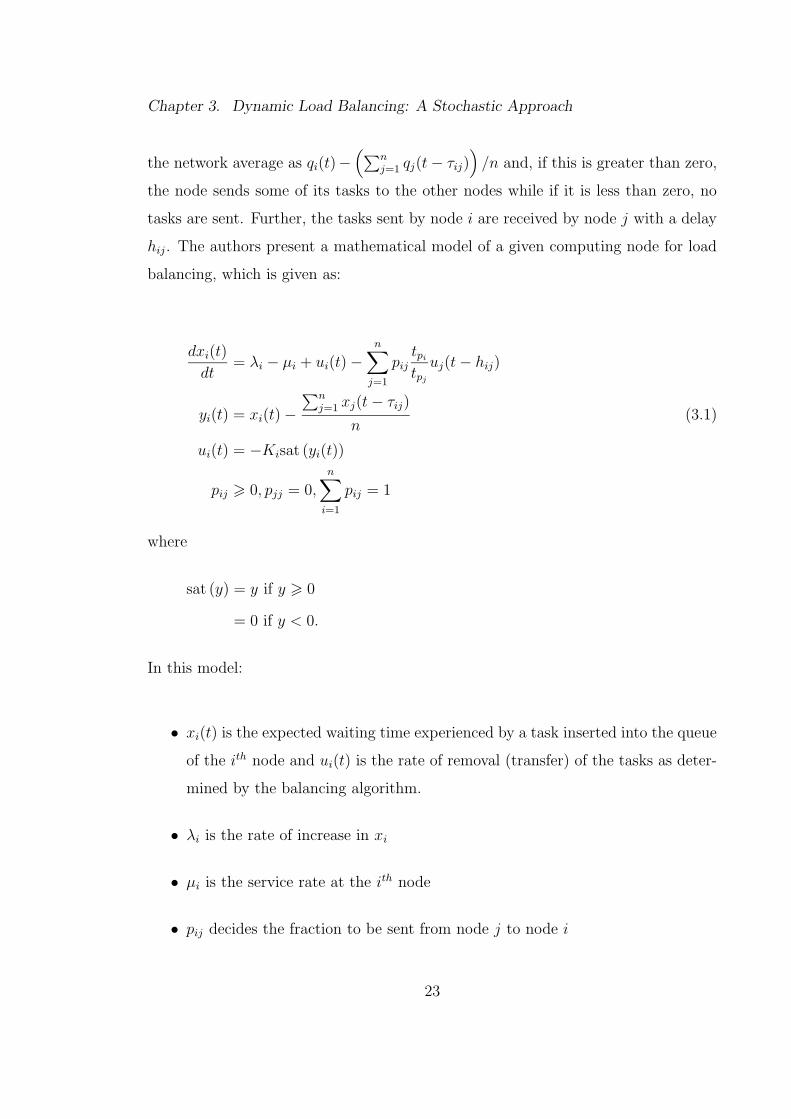
balancing, which is given as:
dxi(t)
dt= λi − µi + ui(t) −
n∑
j=1
pij
tpi
tpj
uj(t − hij)
yi(t) = xi(t) −
∑n
j=1 xj(t − τij)
n(3.1)
ui(t) = −Kisat (yi(t))
pij > 0, pjj = 0,n∑
i=1
pij = 1
where
sat (y) = y if y > 0
= 0 if y < 0.
In this model:
• xi(t) is the expected waiting time experienced by a task inserted into the queue
of the ith node and ui(t) is the rate of removal (transfer) of the tasks as deter-
mined by the balancing algorithm.
• λi is the rate of increase in xi
• µi is the service rate at the ith node
• pij decides the fraction to be sent from node j to node i
23
Chapter 3. Dynamic Load Balancing: A Stochastic Approach
The authors use the local information of the waiting times xi(t), i = 1, .., n to set
the values of the pij such that node j can send tasks to node i in proportion to the
amounts by which node i is below the local average as seen by node j.
3.2 Description of the Stochastic Dynamics
The load balancing problem in the presence of delay can be generically described
as follows. Consider n nodes in a network of geographically-distributed CEs. Com-
putational tasks arrive at each node randomly and tasks are completed according
to an exponential service-time model. In a typical load-balancing algorithm, each
node routinely checks its queue size against other nodes and decides whether or not
to allocate a portion of its load to less busy nodes according to a predefined policy.
Now due to the physical (or virtual) distance between nodes in large-scale distributed
computing systems, communication and load transfer activity among them cannot
be assumed instantaneous. Thus, the information that a particular node has about
other nodes at any time is dated and may not accurately represent the current state
of the other nodes. For the same reason, a load sent to a recipient node arrives at
a delayed instant. In the mean time, the load state of the recipient node may have
considerably changed from what was known to the transmitting node at the time of
load transfer. Furthermore, what makes matters more complex is that these delays
are random. For example, the communication delay is random since the state of the
shared communication network is unpredictable, depending on the level of traffic,
congestion, and quality of service (QoS) attributes of the network. Clearly, the char-
acteristics of the delay depend on the network configuration and architecture, the
type of communication medium and protocol, and on the overall load of the system.
Other factors that contribute to the stochastic nature of the distributed comput-
ing problem include: 1) Randomness and possible burst-like nature of the arrival of
24

Chapter 3. Dynamic Load Balancing: A Stochastic Approach
new job requests at each node from external sources (i.e., from users); 2) Random-
ness of the load-transfer process itself, as it depends on some deterministic law that
may use a sliding-window history of all other nodes (which are also random); and 3)
Randomness in the task completion process at each node. In the next section, we lay
out a queuing model that characterizes the dynamics of the load-balancing problem
described so far.
3.3 A Discrete-time Queuing Model with Delays
Consider n nodes (CEs), and let Qi(t) denote the number of tasks awaiting processing
at the ith node at time t. Suppose that the ith node completes tasks at a rate µi,
and new job requests are assigned to it from external sources (i.e., external users) at
a rate λi. Note that these incoming tasks come from sources external to the network
of nodes and do not include the jobs transferred to a node from other nodes as a
result of load balancing. Let the counting process Ji(t1, t2) denote the number of
such external tasks arriving at node i in the interval [t1, t2]. To capture any possible
burst-like characteristics in the external-task arrivals (as each job request may involve
a large number of computational tasks), we will assume that the process Ji(·, ·) is a
compound Poisson process [29]. That is, Ji(t1, t2) =∑
k:t1<τk≤t2Hk, where τk are the
arrival times of job requests (which arrive according to a Poisson process with rate
λi) and Hk (k = 1, 2 . . .) is an integer-valued random variable describing the number
of tasks associated with the kth job request. We next address the load transfer
between nodes which will allow us to describe the dynamics of the evolution of the
queues.
For the ith node and at its specific load-balancing instants T il , l = 1, 2, . . . , the
node looks at its own load Qi(Til ) and the loads of other nodes at randomly delayed
instants (due to communication delays), and decides whether it should allocate some
25

Chapter 3. Dynamic Load Balancing: A Stochastic Approach
of its load to other nodes, according to a deterministic (or randomized, if so desired)
load-balancing policy. Moreover, at times when it is not balancing its load, it may
receive loads from other nodes that were transmitted at a randomly delayed instant,
governed by the characteristics of the load-transfer delay. With the above descrip-
tion of task assignments between nodes, and with our earlier description of task
completion and external-task arrivals, we can write the dynamics of the ith queue in
differential form as
Qi(t+∆t) = Qi(t)−Ci(t, t+∆t)−∑
j 6=i
Lji(t)+∑
j 6=i
Lij(t−τij(t))+Ji(t, t+∆t), (3.2)
where
• Ci(t, t + ∆t) is a Poisson process with rate µi describing the random number
of tasks completed in the interval [t, t + ∆t]
• Ji(t, t+∆t) is the random number of new (from external sources) tasks arriving
in the same interval, as discussed above
• τij(t) is the delay in transferring the load arriving to node i in the interval
[t, t + ∆t] from node j, and finally
• Lij(t) is the load transferred from node j to node i at the time t.
For any k 6= l, the random load Lkl diverted from node l to node k is gov-
erned by the mutual load-balancing policy a-priorily agreed upon between the two
nodes, which utilizes knowledge of the state of the lth node and the delayed knowl-
edge of the kth node and all the other nodes. More precisely, we assume Lkl(t)4
=
gkl(Ql(t), Qk(t − ηlk(t)), . . . , Qj(t − ηlj(t)), . . .), where for any j 6= k, ηkj(t) = ηjk(t)
is the communication delay between the kth and jth nodes at time t. The function
gkl dictates the load-balancing policy between the kth and lth nodes. One common
26

Chapter 3. Dynamic Load Balancing: A Stochastic Approach
example is
gkl(Ql(t), Qk(t − ηlk(t)), . . . , Qj(t − ηlj(t)), . . .)
= Kkpkl ·
(
Ql(t) − n−1
n∑
j=1
Qj(t − ηlj(t))
)
· u
(
Ql(t) − n−1
n∑
j=1
Qj(t − ηlj(t))
)
,
(3.3)
where u(·) is the unit step function with the obvious convention ηii(t) = 0, and Kk
is a parameter that controls the “strength” or “gain” of load balancing at the kth
(load distributing) node. We will refer to it henceforth as the gain coefficient. In
this example, the lth node simply compares its load to the average over all nodes
and sends out a fraction pkl of its excess load,Ql(t)−n−1∑n
j=1 Qj(t− ηlj), to the lth
node. (Of course we require that∑
k 6=l pkl = 1.) This form of policy has been used
at the University of Tennessee for the FBI project [1, 23]. Finally, the fractions pkl
can be defined in a variety of ways. Here, they are defined as follows:
pkl =1
n − 2
(
1 −Qk(t − ηlk)
∑
i6=l Qi(t − ηli)
)
, (3.4)
where n ≥ 3. In this definition, a node sends a larger fraction of its excess load to a
node with a small load relative to all other candidate recipient nodes. For the special
case when n = 2, pkl = 1, where k 6= l.
3.4 Simulation Results
We have developed a custom-made Monte-Carlo simulation software according to our
queuing model. We utilized actual data from load-balancing experiments (conducted
at the University of Tennessee) pertaining to the number of tasks awaiting processing,
average communication delay, average load-transfer delay, and actual load-balancing
27

Chapter 3. Dynamic Load Balancing: A Stochastic Approach
instants [23]. In the actual experiment, the communication and load-transfer delays
were minimal (due the fact that the PCs were all in a local proximity and benefited
from a dedicated fast Ethernet). Thus, to better reflect cases when the nodes are ge-
ographically distant we synthesized larger delays in communication and load transfer
in our simulations.
0 10 20 30 40 50 600
0.2
0.4
0.6
0.8
TIME, ms
QUE
UE L
ENG
TH
Zero−Delay Case
Queue 1Queue 2Queue 3Tasks Completed
0 10 20 30 40 50 60−0.5
0
0.5
1
TIME, ms
EXCE
SS L
OAD
Queue 1Queue 2Queue 3
Figure 3.1: Top: Queue size in the
ideal case when delays are nonexis-
tent. The queues are normalized by
the total number of submitted tasks
(12000 in this case). The dashed
curves represent the tasks completed
cumulatively in time by each node.
Bottom: Excess queue length for
each node computed as the difference
between each nodes normalized queue
size and the normalized queue size of
the overall system. Note that the
three nodes are balanced at approxi-
mately 15 ms and that all tasks are
completed in approximately 39 ms.
0 10 20 30 40 50 600
0.2
0.4
0.6
0.8
TIME, ms
QUE
UE L
ENG
TH
Deterministic−Delay Case
Queue 1Queue 2Queue 3Tasks Completed
0 10 20 30 40 50 60−0.5
0
0.5
1
TIME, ms
EXCE
SS L
OAD
Queue 1Queue 2Queue 3
Figure 3.2: Similar to Fig. 3.1 but
with a deterministic communication
and load-transfer delays of 8 ms and
16 ms, respectively. In contrast to the
zero-delay case, the three nodes are
balanced at approximately 60 ms and
all tasks are completed shortly after-
wards. Also note that nodes 2 and
3 each execute approximately 40% of
the total tasks, where node 3 executes
only 20% of the total tasks submitted
to the system.
28

Chapter 3. Dynamic Load Balancing: A Stochastic Approach
3.4.1 Effect of Delay
Three CEs were used in the simulations and a standard load-balancing policy [as de-
scribed by (3.3)] was implemented. The PCs were assumed to have equal computing
power (the average task completion time was 10 µs per task), but the initial load
was distributed unevenly among the three nodes as 7000, 4500, and 500 tasks, with
no additional external arrival of tasks (e.g., J1(t1, t2) = 7000 if t1 = 0, 0 < t2 and
zero otherwise). Figure 3.1 corresponds to the case where no communication nor
load-transfer delays are assumed. This case approximates the actual experiment,
where all the computers were within the proximity of each other benefiting from a
dedicated fast Ethernet. Note that the system is balanced at approximately 15 ms
and remains balanced thereafter until all tasks are executed in approximately 39 ms.
We next considered the presence of deterministic communication delay of 8 ms and
a load transfer-delay of 16 ms. The behavior is seen in Fig. 3.2, where it is observed
that the delay prevents load balancing to occur. For example, nodes 2 and 3 each
eventually execute approximately 40% of the total tasks, whereas node 3 executes
only 20% of the total tasks submitted to the system (as seen from the dashed curves
in the top figure in Fig. 3.2). The conclusion drawn here is that the presence of delay
in communication and load transfer seriously disturbs the performance of the load
balancing policy, as each node utilizes “dated” information about the state of the
other nodes as it decides what fraction of its load must be transferred to each of the
other nodes.
To see the effect of the delay randomness on the load balancing performance,
two representative realizations of the performance were generated and are shown in
Figs. 3.3 and 3.4. The average delays were taken as in the deterministic case (i.e.,
8 ms for the communication delay and 16 ms for the load-transfer delay). For the
example considered, it turns out that the performance is sensitive to the realizations
of the delays in the early phase of the load-balancing procedure. For example, it
29

Chapter 3. Dynamic Load Balancing: A Stochastic Approach
0 10 20 30 40 50 60 70 800
0.2
0.4
0.6
0.8
TIME, ms
QUE
UE L
ENG
THRandom−Delay Case
Queue 1Queue 2Queue 3Tasks Completed
0 10 20 30 40 50 60 70 80−0.5
0
0.5
1
TIME, ms
EXCE
SS L
OAD
Queue 1Queue 2Queue 3
Figure 3.3: In this example, the com-
munication and load-transfer delays
are assumed random with average val-
ues of 8 ms and 16 ms, respectively.
Note that the performance is some-
what superior to the deterministic-
delay case shown in Fig. 3.2.
0 10 20 30 40 50 60 70 800
0.2
0.4
0.6
0.8
TIME, ms
QUE
UE L
ENG
TH
Random−Delay Case
Queue 1Queue 2Queue 3Tasks Completed
0 10 20 30 40 50 60 70 80−0.5
0
0.5
1
TIME, ms
EXCE
SS L
OAD
Queue 1Queue 2Queue 3
Figure 3.4: Another realization of the
case described in Fig. 3.3 showing the
variability in the performance from
one realization to another. Load-
balancing characteristics here are in-
ferior to those in Fig. 3.3.
is seen from the simulation results that a deterministic (fixed) delay can lead to a
more severe performance degradation than the case when the delays are assumed
random (with the same mean as the deterministic case). To see the average effect of
the random delay, we calculated the mean queue size and the normalized variance
(normalized by the mean square) over 100 realizations of the queue sample functions,
each with a different set of randomly generated delays. The results are shown in
Figs. 3.5 and 3.6. It is seen from the mean behavior that the randomness in the
delay actually leads, on average, to balancing characteristics (as far as the excess-
load is concerned) that are superior to the case when the delays are deterministic!
However, there is a high level of uncertainty in the queue size, and hence in the load
balancing. It is seen from Fig. 3.5 (dashed curves) that the average total number
of tasks completed by each node continues to increase well beyond 60 ms, which
is inferred from the positive slope of the dashed curves. This indicates that in
30

Chapter 3. Dynamic Load Balancing: A Stochastic Approach
comparison to the deterministic-delay case, the system requires 1) almost twice as
long as the zero-delay case to complete all the tasks and 2) a longer time to complete
all the tasks than the deterministic-delay case.
0 10 20 30 40 50 600
1000
2000
3000
4000
5000
6000
7000
TIME,ms
Que
ue L
engt
h
Queue 1Queue 2Queue 3mean tasks completed
Figure 3.5: The empirical average
queue length using 100 realizations
of the queues for each node (solid
curves). The dashed curves are the
empirical average of the number of
tasks performed by each node cumula-
tively in time normalized by the total
number of tasks submitted to the sys-
tem. Only 87% of the total tasks are
completed within 60 ms.
0 10 20 30 40 50 600
5
10
15
20
25
30
35
40
TIME, msVa
rianc
e in
the
Que
ue le
ngth
Queue 3
Figure 3.6: The empirical variance
of the queue length normalized by
the mean-square values. Observe the
high-degree of uncertainty in the low-
est queue as well as the variability at
large times, which is indicative of the
fact that nodes continue to exchange
tasks back and forth, perhaps unnec-
essarily.
3.4.2 Interplay Between Delay and the Gain Coefficient K
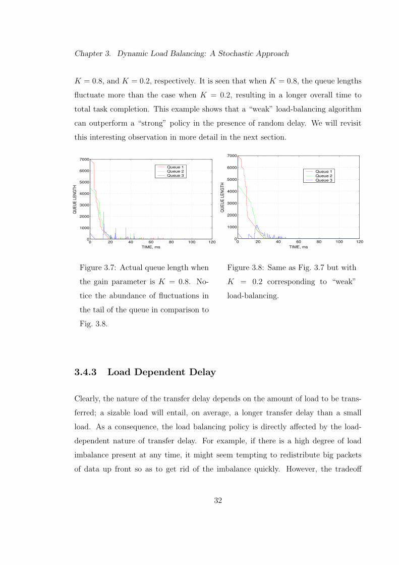
We finally consider the effect of varying the gain parameter K on the performance
of load balancing (assume that K1 = K2 = K3 ≡ K). Figures 3.7, 3.8 show the
the performance under two cases corresponding to a large and small gain coefficient,
31
Chapter 3. Dynamic Load Balancing: A Stochastic Approach
K = 0.8, and K = 0.2, respectively. It is seen that when K = 0.8, the queue lengths
fluctuate more than the case when K = 0.2, resulting in a longer overall time to
total task completion. This example shows that a “weak” load-balancing algorithm
can outperform a “strong” policy in the presence of random delay. We will revisit
this interesting observation in more detail in the next section.
0 20 40 60 80 100 1200
1000
2000
3000
4000
5000
6000
7000
TIME, ms
QUE
UE L
ENG
TH
Queue 1Queue 2Queue 3
Figure 3.7: Actual queue length when
the gain parameter is K = 0.8. No-
tice the abundance of fluctuations in
the tail of the queue in comparison to
Fig. 3.8.
0 20 40 60 80 100 1200
1000
2000
3000
4000
5000
6000
7000
TIME, ms
QU
EUE
LEN
GTH
Queue 1Queue 2Queue 3
Figure 3.8: Same as Fig. 3.7 but with
K = 0.2 corresponding to “weak”
load-balancing.
3.4.3 Load Dependent Delay
Clearly, the nature of the transfer delay depends on the amount of load to be trans-
ferred; a sizable load will entail, on average, a longer transfer delay than a small
load. As a consequence, the load balancing policy is directly affected by the load-
dependent nature of transfer delay. For example, if there is a high degree of load
imbalance present at any time, it might seem tempting to redistribute big packets
of data up front so as to get rid of the imbalance quickly. However, the tradeoff
32

Chapter 3. Dynamic Load Balancing: A Stochastic Approach
here is that the sizable load takes much longer to reach the destination node, and
hence, the overall computation time will inevitably increase. Thus,we would expect
the gain coefficient K to play an important role in cases when transfer delay is load
dependent. Since the balancing is done frequently, it is intuitively obvious that we
would be better of if we were to select K conservatively. To address this issue quanti-
tatively, we will need to develop a model for the load-dependent transfer delay. This
is done next.
We propose to capture the load-dependent nature of the random transfer delay
τij by requiring that its average value θij(t), assumes the following form
θij(t) = dmin −1 + exp([(Lij(t)dβ)]−1)
1 − exp([(Lij(t)dβ)]−1), (3.5)
where dmin is the minimum possible transfer delay (its value is estimated as 9 ms in
this paper), d is a constant (equal to 0.082618), β is a parameter which characterizes
the transfer delay (selected as 0.04955). Moreover, we will assume that conditional
on the size of the load to be transferred, the random delay τij is uniformly-distributed
in the interval [0,2θij(t)]. This model assumes that up to some threshold, the de-
lay is constant (independent of the load size) that is dependent on the capacity of
the communication medium. Beyond this threshold, however, the average delay is
expected to increase monotonically with the load size. The parameters d and b are
selected so that the above model is consistent with the overall average delay for all
the actual transfers that occurred in the previous simulations.
The load-dependent transfer delay versus the load is shown in the Fig. 3.9. The
transfer delay for the loads sent from node 1 to node 3 (top) and from node 2 to node
3 (bottom) over the period of execution time is shown in Fig. 3.10. With the average
communication delay being equal to 8 ms (as before) and the transfer delay made
load dependent, according to the model described in (3.5), one realization of the
performance for K = 0.5 was generated and it is shown in Figure 3.11. As expected,
the performance deteriorates beyond the case corresponding to a fixed transfer delay.
33

Chapter 3. Dynamic Load Balancing: A Stochastic Approach
0 100 200 300 400 500 600 700 800 900 100010
10.2
10.4
10.6
10.8
11
11.2
No. of tasks
Ave
rage
Tra
nsfe
r Del
ay, m
s
Figure 3.9: Transfer Delay changes
significantly for big loads.
0 5 10 15 20 25 30 35 400
20
40
60
80
TIME, ms
Del
ay, m
s
0 5 10 15 20 25 30 35 400
50
100
150
TIME, ms
Del
ay, m
sFigure 3.10: Transfer Delay Varia-
tion for a particular realization of the
queues
For example, we see from the figure that a load sent by node 1 at around 5ms arrives
at node 3 approximately 50 ms later, thereby bringing more fluctuations to the tail
to the queues. The average effect (over 50 realizations) of this delay model for two
different gain parameters (K = 0.1 and K = 0.9) can be seen in Figs. 3.12 and 3.13.
When K = 0.9, the queue is fluctuating beyond t = 80ms while when K = 0.1, all
the tasks are completed at approximately 60ms. The optimal value of K for this
delay model was found to be equal to K = 0.06 and the overall completion time in
this case was 54.85 ms. The variation of the overall completion time with respect to
the gain coefficient is shown in Table 3.1.
It is clearly seen that the required time for completion of all tasks (in the sys-
tem) is significantly larger than the time required to execute 95% of the assigned
tasks. The difference increases with higher values of K. This is due to the fact
that even when all the queues are almost depleted of tasks, they continue to execute
the balancing policy. As a result, small amount of tasks (e.g., one or two) are sent
from one node to other nodes and vice versa. This unnecessary task-swapping sig-
34

Chapter 3. Dynamic Load Balancing: A Stochastic Approach
0 10 20 30 40 50 600
1000
2000
3000
4000
5000
6000
TIME, ms
QU
EUE
LEN
GTH
Realization of the Load Dependent Random−Delay Case
Queue 1Queue 2Queue 3Tasks completed
Figure 3.11: Queue is more unsta-
ble than in the case of the load inde-
pendent delay case for the same gain
K = 0.5
0 10 20 30 40 50 60 70 800
1000
2000
3000
4000
5000
6000
7000
TIME, ms
QU
EUE
LEN
GTH
Mean Realization of the Load Dependent Random−Delay Case
Queue 1Queue 2Queue 3Tasks completed
Figure 3.12: With K = 0.1 execution
time is approximately 60 ms
0 10 20 30 40 50 60 70 800
1000
2000
3000
4000
5000
6000
7000
TIME, ms
QU
EUE
LEN
GTH
Mean Realization of the Load Dependent Random−Delay Case
Queue 1Queue 2Queue 3Tasks completed
Figure 3.13: With K = 0.9, the
queues are changing even at 80ms
nificantly increases the transfer delay, therefore increasing the overall computational
time. Further, the tiny amount of tasks keep moving back and forth. This phe-
35

Chapter 3. Dynamic Load Balancing: A Stochastic Approach
Table 3.1: Dependence of the load-balancing performance on the gain coefficeint K.
Gain(K) Task Completion Time(in
ms)
Time to Execute 95 percent
of tasks(in ms)
0.01 62.53 41.80
0.02 61.44 42.86
0.03 59.68 42.59
0.04 57.27 41.98
0.05 56.79 41.35
0.06 54.85 41.99
0.07 56.04 42.49
0.08 59.68 41.56
0.09 62.53 41.81
0.1 61.10 42.18
0.2 65 43.38
0.3 63.40 46.2
0.4 78.313 53.33
0.5 > 80 55.21
nomenon is clearly depicted in Figs. 3.6 where the minute fluctuations are evident
near the tail of the queues.
3.5 Summary and Conclusions
Whenever there are tangible communication limitations between nodes in a dis-
tributed system, possibly with geographically distant CEs, we must take a totally
new look at the problem of load balancing. In such cases, the presence of non-
36

Chapter 3. Dynamic Load Balancing: A Stochastic Approach
negligible random delays in inter-node communication and load transfer can signif-
icantly alter the expected performance of existing load-balancing strategies. The
load-balancing problem must be viewed as a stochastic system, whose performance
must be evaluated statistically. More importantly, the policy itself must be devel-
oped with appropriate statistical performance criteria in mind. Thus, if we design a
load-balancing policy under the no-delay or fixed-delay assumptions, the policy will
not perform as expected in a real situation when the delays are non-zero or random.
A load-balancing policy must be designed with the stochastic nature of the delay in
mind.
Monte-Carlo simulation indicates that the presence of delay (deterministic or ran-
dom) can lead to a significant degradation in the performance of a load-balancing
policy. Moreover, when the delay is stochastic, this degradation is worsened, lead-
ing to extended cycles of unnecessary exchange of tasks (or loads), back and forth
between nodes, leading to extended overall delays and prolonged task-completion
times. One way to remedy such a problem is to weaken the load-balancing mecha-
nism (or discourage) appropriately. this action makes the load balancing policy in
the presence of random delays “less reactionary” to changes in the load distribution
within the system. This, in turn, reduces the sensitivity of the load-balancing process
to inaccuracies in the state-of-knowledge of each node about the load distribution
in the remainder of the system caused by communication limitations. We look into
these interesting issues in the following chapter.
37

Chapter 4
Discrete-Time Load Balancing
In a distributed computing environment with a high communication cost, limiting
the number of balancing instants results in a better performance than the case where
load balancing is executed continuously. Therefore, finding the optimal number of
balancing instants and optimizing the performance over the inter-balancing time
and over the load-balancing gain becomes an important problem. In this chapter
we show that the choice of the balancing strategy is an optimization problem with
respect to the choice of the gain parameter. We discuss the performance of a single
load-balancing strategy on a real distributed physical system and the performance
is compared to our simulation predictions.
The contents of this chapter have been taken from [27, 28]. This chapter is or-
ganized as follows. In Section 4.1 we present the motivation behind limiting the
balancing instants. In Section 4.2, the results of Monte-Carlo simulations for single
and double load-balancing strategies are presented and analyzed. Section 4.3 dis-
cusses the performance of our single-load balancing strategy on a physical wireless
3-node network, while simulation results for this case is presented in Section 4.4.
Finally, we conclude the chapter in Section 4.5.
38
Chapter 4. Discrete-Time Load Balancing
4.1 Motivation
In chapter 4, we looked at the problem of dynamic load balancing using a dynamical
model that captures the stochastic delays of the distributed system. In the ideal case
where the communication and load-transfer delays are small (as in a fast Ethernet
environment) and the time required to implement the load-balancing policy is also
negligible, the best performance (minimizing the waiting times associated with all
CEs) is obtained when the load balancing is executed almost continuously without
any reservation. Namely, at almost every instant, each CE compares its queue size to
the average queue size of the network and distributes all its excess load to other nodes.
Every other node also follows a similar policy. However, in a practical setting such
a strategy has two main disadvantages: 1) the implementation of the load balancing
policy on a continuous basis can drain the computational resources of each CE; and
2) excessive load balancing, both in frequency and strength, can lead to timely and
possibly unnecessary exchange of loads between CEs. This means that valuable time
may be unduly wasted exchanging loads back and forth between nodes (as the system
is diligently attempting to balance the queues) while this time could have been used
to actually execute the tasks submitted! In particular, we showed that the strength
of the load-balancing policy must be reduced in a delayed environment to avoid any
“over-reaction” consequences that may arise due to such delay factors.
In a more practical setting, the continuous implementation of load balancing,
as we stated earlier, can be very costly (wasteful of computational resources) and
more importantly, it can inflict an additional delay, namely, the time needed to
implement the load balancing policy. Thus, there is an inherent tradeoff between
the strength and frequency of load balancing on one hand, and the need to conserve
computational resources used in implementing any load-balancing policy. Motivated
by such a fundamental tradeoff, in this chapter we investigate whether limiting the
number of load balancing instants while optimizing the strength of the load balancing
39

Chapter 4. Discrete-Time Load Balancing
and the actual load-balancing instants is a feasible solution to the problem of load
balancing in a delay-limited environment. We address the performance of such a
potentially computationally-efficient load-balancing strategy.
4.2 Simulation Results
The queuing model and the balancing algorithm described in Chapter 4 have been
used to generate all the simulations that will be discussed here. Consider a cluster
of three nodes with equal computing power (i.e., the task completion rates, µi, i =
1, 2, 3, are all the same), and let us assume that each node is allowed to execute load
balancing at only two scheduling times. We assume that the average task completion
time is 10 µs per task, and the load-balancing policy is implemented according to
the policy described in the previous section. The initial load for these experiments
was distributed unevenly among the three nodes as 7000, 4500, and 500 tasks, with
no additional external arrival of tasks (in this thesis we only consider the zero-input
response).
Some of our earlier experimental results that motivated the present study are
summarized in Fig. 4.1. The top graph in this figure shows the empirical average
of the queue size (dashed curves show the number tasks cumulatively performed).
It is seen that approximately only 87% of the total tasks were completed within 60
ms. The fact that the total number of tasks performed by each CE are not the
same indicates that load-balancing has not been effective (since all nodes have the
same computing capability), which is attributed mainly to the presence of delay.
To have better insight into the time elapsed before all the tasks are computed, we
generated the empirical variance of the queues, as shown by the bottom graph in
Fig. 4.1. The graph shows a high-degree of uncertainty in the smallest queue and,
more importantly, near the tail of the queues (beyond 30 ms). We observed that even
40

Chapter 4. Discrete-Time Load Balancing
in the fastest completion period, 95% of the tasks were completed around 15 ms faster
then the time taken to complete the last 5% the tasks. This is an indicator that the
nodes are continuing to exchange tasks back and forth near the tail of the queue even
when load-balancing seems unnecessary. The more often we try to equalize the work
load between the nodes, the more often portions of loads are transferred between the
CEs. As a result, the CEs are not able to complete their assigned tasks by the time
of the new load balancing policy execution. The net effect is that loads are bouncing
between the nodes with little actual work being performed.
4.2.1 Single Load-balancing Strategy
We now present the results for the case when load-balancing is implemented at a
single instant only per node. We assumed initial loads of Q1(0) = 7000, Q2(0) =
4500, and Q3(0) = 500, and an average communication and load-transfer delays of
8 ms (corresponding to relatively short load balancing transfer delays). The results
showed that the optimal value for the load-balancing strength parameter Kopt is
0.8 ms, the optimal load balancing instant tbal1 is 0.02 ms, and the corresponding
completion time tcompl is 47.57 ms, as seen in Fig. 4.2 (top). Now from the bottom
graph in Fig. 4.2, we can see that the queue lengths change abruptly as a result of
load-balancing events associated with the three nodes (a total of six transitions and
two transitions per node in this case: one transition when a node transmits tasks to
other nodes, and once when it receives the tasks that were sent to it). The group of
increasing curves represents the tasks completed cumulatively in time by each node.
We also noticed that when K ranges between 0.4 and 0.9, the completion time first
decreases to a minimum of 47.57 ms, and then increases to 55 ms. The optimal range
of the gain parameter is between 0.7 and 0.8. Within this range tbal1 is changing from
0.01 ms to 3.68 ms. Therefore, for relatively small communications delays, we can
execute the load balancing policy either before the present states of the neighboring
41

Chapter 4. Discrete-Time Load Balancing
0 20 40 60 80 100 1200
1000
2000
3000
4000
5000
6000
7000
TIME, ms
QU
EU
E L
EN
GTH
Mean Realization of the Random−Delay Case
Queue 1Queue 2Queue 3mean tasks completed
0 20 40 60 80 100 1200
20
40
60
80
100
120
TIME, ms
NO
RM
ALI
ZED
VA
RIA
NC
E
VARIANCE
Queue1Queue 2Queue 3
Figure 4.1: Top: The empirical mean queue length using 100 realizations of the
queues for each node (solid curves). Dashed curves are empirical averages of the
tasks performed by each node cumulatively in time. Bottom: The empirical variance
of the queue length normalized by the mean-square values.
nodes are known, or after we receive this information. Nevertheless, there is a tradeoff
involved in choosing one choice over the other. If completion time is the primary
optimization goal, then it is advantageous to execute the load balancing policy at the
42
Chapter 4. Discrete-Time Load Balancing
very beginning, combined with a large value of the gain parameter. However, this
comes at the price of sensitivity to any delay in executing the load balancing. For
example, if the execution is delayed to just before the time when communication from
other nodes arrive, then the completion is significantly prolonged, as can be seen from
the peak near tbal1 = 0.6 ms. On the other hand, if maintaining a stable (i.e., less
sensitivity to error in the execution time) is sought, then it would be advantageous
to execute the load balancing after receiving information from the neighboring nodes
at a slight price of prolonged task completion time.
Next we consider a case where the delays are relatively long, both in communi-
cation and load transfer. As can be seen from the top plot in Fig. 4.3, the shortest
completion time possible is approximately 52 ms for tbal1 = 0.01 ms and the optimal
value of K is found to be 0.65. Like in the above scenario, there is no reason for CEs
to wait for the information to reach them, because if they do valuable time will be
wasted (due to the large communication delay) since one node is idle. Thus, in this
case, “informed” load balancing does not render efficiency. Moreover, the optimal
value of the balancing strength parameter has to be smaller compared to the case
with short load-transfer delays. The reason is that in the present situation it will
take longer for most of the information to reach its destination, and consequently,
the overall completion time will increase. In addition, our simulations show that
even with the optimal value of K, the task-completion time cannot reach the one
corresponding to the short-delay case considered earlier. From the bottom plot in
the same figure we can see that CE1 and CE2 complete their work 5 ms after CE3.
Thus, the system’s load was not totally balanced.
To investigate the relationship between the initial load distribution and the op-
timal values for the system parameters, we considered a case where the initial loads
are almost equally distributed between the nodes. In particular, we considered
Q1(0) = 7000, Q2(0) = 6500, and Q3(0) = 6000. For this setting, the shortest
43

Chapter 4. Discrete-Time Load Balancing
0 1 2 3 4 5 47
48
49
50
51
52
53
54
55
56
INSTANTS FOR FIRST BALANCING(ms)
CO
MP
LETI
ON
TIM
E(m
s)
0 10 20 30 40 500
1000
2000
3000
4000
5000
6000
7000
TIME, ms
QU
EU
E L
EN
GTH
Queue 1Queue 2Queue 3Done By 1Done By 2Done By 3
Figure 4.2: Optimal single load-balancing scheduling for the short-delay case. Top:
completion time vs. load-balancing instant, tbal1; Bottom: queue lengths and cumu-
lative tasks completed by each node.
completion time was 66.51 ms at K = 0.725 and for tbal1 = 0.63 ms. These values
are very close to the ideal case when no time delays are present and the minimum
completion time for a total of 19500 tasks is 65 ms. From our empirical measure-
ments we can conclude that when we have only one load-balancing execution per
44

Chapter 4. Discrete-Time Load Balancing
0 2 4 6 8 1051
52
53
54
55
56
57
58
INSTANTS FOR FIRST BALANCING(ms)
CO
MP
LETI
ON
TIM
E(m
s)
Balancing Instant
0 10 20 30 40 500
1000
2000
3000
4000
5000
6000
7000
TIME, ms
QU
EU
E L
EN
GTH
Queue 1Queue 2Queue 3Done By 1Done By 2Done By 3
Figure 4.3: Single load-balancing scheduling for the long-delay case. Top: completion
time as a function of tbal1; Bottom: queue evolution and the cumulative tasks done
by each node.
node in a small-delay environment, the best time to implement the load balancing is
almost right at the beginning with a relatively large K (that actually depends on the
initial load distribution). For the longer-delay case, however, K has to be decreased.
45

Chapter 4. Discrete-Time Load Balancing
4.2.2 Double Load-balancing Strategy
Next, we consider a strategy for which a second load balancing instant, denoted by
tbal2, is allowed for each node. From the point of view of each node, tbal2 can be
chosen using several options. For example, tbal2 can be chosen just after the first
load balancing instant, between the moments in which the nodes are receiving loads
from their neighbors, or at the end of the load exchange. If we choose Q1(0) = 7000,
Q2(0) = 4500, Q3(0) = 500, an average communication delay of 0.8 ms, and a similar
average load-transfer delay, then the best tcompl is found to be 43.15 ms, which occurs
when tbal1 = 0.01 ms and tbal2 = 0.02 ms with K = 0.6. A similar completion time
can be achieved by executing the two load-balancing instants at a later time, after
the nodes have received information. We found that this requires two load balancing
instants following each other. In particular, our experiment shows that tbal1 = 3.87
and tbal2 = 3.88 yields one of the best completion times.
From the top plot in Fig. 4.4 we see that balancing in the beginning of the process
leads to shorter completion times. The same plot indicates that execution of the load
balancing within the range 0.03–2 ms is sensitive to error in the scheduling time. In
particular, a small deviation of tbal leads to a substantial increase in completion time.
This time interval coincides with the time when every node receives information from
its neighbors in a random way. Therefore, reliable load balancing is not possible
during this time interval due to the communication delays. For the same reason,
when K = 0.8, the best execution strategy is to execute the first load balancing
policy right at the beginning with tbal1 = 0.01 ms and after that to wait until each
one of the nodes received information from its neighbors before executing the second
load balancing, as seen from Fig. 4.4 (middle). The completion time achieved in
this case is 45 ms. Thus, qualitatively speaking, when we have two load-balancing
instants in a small-delay environment, the optimal way to place them is either in the
beginning, or immediately after the CEs have completed the information exchange.
46
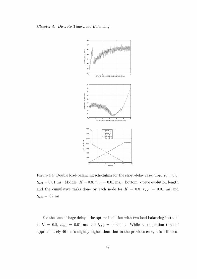
Chapter 4. Discrete-Time Load Balancing
0 5 10 1541
42
43
44
45
46
47
48
INSTANTS FOR SECOND LOAD BALANCING(ms)
CO
MP
LETI
ON
TIM
E(m
s)
0 10 20 30 40 50 6044
46
48
50
52
54
56
58
60
62
INSTANTS FOR SECOND LOAD BALANCING (ms)
CO
MP
LETI
ON
TIM
E (m
s)
0 10 20 30 40 500
1000
2000
3000
4000
5000
6000
7000
TIME, ms
QU
EU
E L
EN
GTH
Queue 1Queue 2Queue 3Done By 1Done By 2Done By 3
Figure 4.4: Double load-balancing scheduling for the short-delay case. Top: K = 0.6,
tbal1 = 0.01 ms,; Middle: K = 0.8, tbal1 = 0.01 ms, ; Bottom: queue evolution length
and the cumulative tasks done by each node for K = 0.8, tbal1 = 0.01 ms and
tbal2 = .02 ms
For the case of large delays, the optimal solution with two load balancing instants
is K = 0.5, tbal1 = 0.01 ms and tbal2 = 0.02 ms. While a completion time of
approximately 46 ms is slightly higher than that in the previous case, it is still close
47

Chapter 4. Discrete-Time Load Balancing
0 5 10 15 20 25 3045
46
47
48
49
50
51
52
53
54
INSTANTS FOR SECOND LOAD BALANCING (ms)
CO
MP
LETI
ON
TIM
E (m
s)
0 10 20 30 40 50 600
1000
2000
3000
4000
5000
6000
7000
TIME, ms
QU
EU
E L
EN
GTH
Queue 1Queue 2Queue 3Done By 1Done By 2Done By 3
Figure 4.5: Double load-balancing scheduling for the long-delay case. Top: K = 0.5,
tbal1 = 0.01 ms; Bottom: queue length evolution and the cumulative tasks done by
each node.
to its optimal value. We see from Fig. 4.5 (top) that the two instants are in the
beginning of the process. Long delays will cause nodes to use dated information
to determine the load redistribution. We also found that the value of Kopt is lower
compared to the short-delay case. The long time delays require smaller values of Kopt
48

Chapter 4. Discrete-Time Load Balancing
0.1 0.2 0.3 0.4 0.5 0.6 0.7 0.8 0.9 140
45
50
55
60
65
GAIN PARAMETER(K )
MIN
IMU
M C
OM
PLE
TIO
N T
IME
(ms)
Small Delay Case
0.1 0.2 0.3 0.4 0.5 0.6 0.7 0.8 0.9 145
50
55
60
65
70
GAIN PARAMETER (K)
MIN
IMU
M C
OM
PLE
TIO
N T
IME
(ms)
LARGE DELAY CASE
Figure 4.6: Double load-balancing scheduling showing the task completion time as a
function of the load-balancing strength parameter K. Top: small-delay case; Bottom:
large-delay case.
because it takes longer time to transfer larger packets of data between the nodes, and
selecting a high value for K will be “over-reactive.” For example, for K = 0.9 the
cluster behavior is unstable and small perturbations in the load balancing instant
cause increase in the completion time. The behavior of the double-balancing case is
summarized in Fig. 4.6. The top plot shows the dependence of the minimum tcompl
49

Chapter 4. Discrete-Time Load Balancing
as a function of the load-balancing strength parameter K for small delays, and the
bottom plot shows the same dependency for the long-delay case.
4.3 Experimental Results
We have developed an in-house testbed 1 to study the effects of the gain parameter
K as well as the selection of the load-balancing instant. The details of the system
are described below.
4.3.1 Description of the experiments
The experiments were conducted over a wireless network using an 802.11b access
point. The testing was completed on three computers: a 1.6 GHz Pentium IV
processor machine (node 1) and two 1 GHz Transmeta Processor machines (nodes 2
& 3). To increase communication delays between the nodes (so as to bring the test-
bed to setting that resembles a realistic setting of a busy network), the access point
was kept busy by third party machines which continuously downloaded files. The
application used to illustrate the load balancing process was matrix multiplication,
where one task has been defined as the multiplication of one row by a static matrix
duplicated on all nodes (3 nodes in our experiment). The size of the elements in each
row was generated randomly from a specified range which made the execution time
of a task variable. On average, the completion time of a task was 525 ms on node 1,
and 650 ms on the other two nodes. As for the communication part of the program,
UDP was used to exchange queue size information among the nodes and TCP was
used to transfer the data or tasks from one machine to another.
1This implementation [28] is done by Mr. J. Ghanem, a graduate student in the EECE
Department at UNM.
50

Chapter 4. Discrete-Time Load Balancing
In the first set of experiments, the gain parameter K was set to 1. Each node
was assigned a certain number of tasks according to the following distribution: Node
1 was assigned 60 tasks, node 2 was assigned 30 tasks, and node 3 was assigned 120
tasks. The information exchange delay (viz., communication delay) was on average
850 ms. Several experiments were conducted for each case of the load-balancing
instant and the average was calculated using five independent realizations for each
selected value of the load-balancing instant. In the second set of experiments, the
load balancing instant was fixed at 1.4 s, and the initial distribution of tasks was as
follows: 60 tasks were assigned to node 1, 150 tasks were assigned to node 2, and 10
tasks were assigned to node 3. The information exchange delay was 322 ms and the
data transfer delay per task was 485 ms.
4.3.2 Discussion of results
The results of the first set of experiments show that if the load balancing is performed
blindly, as in the onset of receiving the initial load, the performance is poorest. This
is demonstrated by the relatively large average completion time (namely 45 ∼ 50 s)
when the balancing instant is prior to the time when all the communication between
the CEs have arrived (namely when tb is approximately below 1s), as shown in
Fig. 4.7. Note that the completion time drops significantly (down to 40 s) as tb
begins to approximately exceed the time when all inter-CE communications have
arrived (e.g., tb > 1.5s). In this scenario of tb, the load balancing is done in an
informative fashion, that is, the nodes have knowledge of the initial load of every
CE. Thus, it is not surprising that the load balancing is more effective than the case
the load balancing is performed on the onset of the initial load arrival for which the
CEs have not yet received the state of the other CEs. Finally, we observe that as
tb increases farther beyond the time all the inter-CE communications arrive (e.g.,
tb > 5s), then the average completion time begins to increase. This occurs precisely
51

Chapter 4. Discrete-Time Load Balancing
because any delay in executing the load balancing beyond the arrival of the inter-CE
communications time would enhance the possibility that some CEs will run out of
tasks in the period before any transferred load arrives to it.
30
35
40
45
50
55
0 1 2 3 4 5 6 7 8BALANCING INSTANT (s)
AV
ER
AG
E C
OM
PLE
TIO
N T
IME
(s)
Figure 4.7: Average total task-completion time as a function of the load-balancing
instant. The load-balancing gain parameter is set at K = 1. The dots represent
the actual experimental values and the solid curve is a best polynomial fit. This
convention is used throughout Fig. 4.10
.
Next we examine the size of the loads transferred as a function of the instant
at which the load balancing is executed, as shown in Fig. 4.8. This behavior will
show that the dependence of the size of the total load transferred on the “knowledge
state” of the CEs. It is clear from the figure that for load-balancing instants up to
approximately the time when all CEs have accurate knowledge of each other’s load
states, the average size of the load assigned for transfer is unduly large. Clearly, this
seemingly ”uninformed” load balancing leads to another imbalance situation, which,
in turn, leads to suboptimal total task completion times, as confirmed by Fig. 4.7.
The results of the second set of experiments indeed confirm our prediction that
52

Chapter 4. Discrete-Time Load Balancing
40
60
80
100
120
140
0 1 2 3 4 5 6 7 8BALANCING INSTANT (s)
NU
MB
ER
OF
TA
SK
S
Figure 4.8: Average total excess load decided by the load-balancing policy to be
transferred (at the load-balancing instant) as a function of the balancing instant.
The load-balancing gain parameter is set at K = 1.
60
70
80
90
100
110
120
0.2 0.4 0.6 0.8 1GAIN, K
AV
ER
AG
E C
OM
PLE
TIO
N T
IME
(s)
Figure 4.9: Average total task-completion time as a function of the balancing gain.
The load-balancing instant is fixed at 1.4 s.
when communication and load-transfer delays are prevalent, the load-balancing gain
must be reduced to prevent “overreaction.” This behavior is shown in Fig. 4.9,
which demonstrates that the optimal performance is achieved not at the maximal
gain (K = 1) but when K is approximately 0.8. This is a significant result as it
53

Chapter 4. Discrete-Time Load Balancing
0
20
40
60
80
0.2 0.4 0.6 0.8 1GAIN, K
NU
MB
ER
OF
TA
SK
S
Figure 4.10: Average total excess load decided by the load-balancing policy to be
transferred (at the load-balancing instant) as a function of the balancing gain. The
load-balancing instant is fixed at 1.4 s.
is contrary to what we would expect in a situation when the delay is insignificant
(as in a fast Ethernet case), where K = 1 yields the optimal performance. Figure
4.10 shows the dependence of the total load to be transferred as a function of the
gain. A large gain (near unity) results in a large load to be transferred, which, in
turn, leads to a large load-transfer delay. Thus, large gains increase the likelihood
of a node (that may not have been overloaded initially) to complete all its load and
remain idle until the transferred load arrives. This would clearly increase the total
average task completion time, as confirmed earlier by Fig. 4.9.
4.4 Simulation Results
We used our Monte-Carlo simulation algorithm to simulate the queues described in
Section 4.3. We assigned the initial distribution of the workload among the three
nodes same as in the experiments and also set the mean communication delay and
54

Chapter 4. Discrete-Time Load Balancing
the mean transfer delay per task according to the statistics obtained from the exper-
iments. In particular, we have generated the simulated versions of Figures 1 through
3, which are shown below. It is observed that the general characteristics of the curves
are very similar which validates the correspondence between the stochastic queuing
model and the experimental setup.
0 1 2 3 4 5 6 7 830
35
40
45
50
55
60
AVER
AGE
COM
PLET
ION
TIM
E (s
)
BALANCING INSTANT (s)
Figure 4.11: Simulation results for the average total excess load decided by the load-
balancing policy to be transferred (at the load-balancing instant) as a function of
the balancing instant. The load-balancing gain parameter is set at K = 1.
4.5 Conclusions
Our simulations indicate that with a double-load-balancing strategy, it is possible to
achieve improved overall performance, measured by the completion time of the total
tasks in the system, in comparison to the single-load-balancing strategy. In either
case, a performance almost comparable to the continuous-load-balancing strategy can
be achieved. The optimal selection of the load-balancing instants is shown to be in
the beginning of the work process with the provision that the gain parameter should
55

Chapter 4. Discrete-Time Load Balancing
0 1 2 3 4 5 6 7 8
40
60
80
100
120
140
BALANCING INSTANT (s)
NU
MBE
R O
F TA
SKS
Figure 4.12: Simulation results for the average total excess load decided by the load-
balancing policy to be transferred (at the load-balancing instant) as a function of
the balancing instant. The load-balancing gain parameter is set at K = 1.
0 0.1 0.2 0.3 0.4 0.5 0.6 0.7 0.8 0.9 155
60
65
70
75
80
85
90
95
100
GAIN, K
AVER
AGE
COM
PLET
ION
TIM
E (s
)
Figure 4.13: Simulation results for the average total task-completion time as a func-
tion of the balancing gain. The load-balancing instant is fixed at 1.4 s.
be selected more conservatively as the delay becomes more pronounced. However,
if the delays are relatively small, it is possible to delay the execution of the load
balancing until the information about the state of other nodes is collected. This
“better informed” balancing will have the advantage of reduced sensitivity to errors
56

Chapter 4. Discrete-Time Load Balancing
in the selection of load-balancing instants.
We have also performed experiments to investigate the performance of a load
balancing policy that involves redistributing the load of the nodes only once af-
ter a large load arrives at the distributed system. Our experimental results (using
a wireless LAN) and simulations both indicate that in distributed systems where
communication and load-transfer delays are tangible, it is best to execute the load
balancing after each node receives communications from other nodes regarding their
load states. In particular, our results indicate that the loss of time in waiting for
the inter-node communications to arrive is overcompensated by the informed nature
of the load balancing. Moreover, the optimal load-balancing gain turns out to be
less than unity, contrary to systems that do not exhibit significant latency. In delay
infested systems, a moderate balancing gain has the benefit of reduced load-transfer
delays, as the fraction of the load to be transferred is reduced. This in turn, will
result in a reduced likelihood of certain nodes becoming idle as soon as they are
depleted of their initial load.
57

Chapter 5
Stochastic Analysis of the Queuing
Model: A Regeneration Approach
Motivated by the fact that we are dealing with an optimization problem, in which we
wish to optimize the load-balancing gain to minimize the average completion time,
in this chapter we will present a novel regenerative approach that will fit the queuing
model described in Chapter 4, with two nodes where a one-shot balancing is done.
The model for the 2-nodes case can be used as a building block to model n-nodes
system, which is not covered in this thesis. The concept of regeneration has proven
to be a powerful tool in the analysis of complex stochastic systems [30, 31, 29]. In
particular, regeneration has been used at different levels to analyze the behavior
of queuing system that arise in communication networks [32, 33, 34]. The analysis
presented in this chapter is not fundamentally limited to the choice of a particular
balancing policy and the idea of the exposition is to show viability of the approach
in analyzing the complex queuing model involved. Consider n nodes in a network of
geographically-distributed CEs with some random initial workload. We are interested
in knowing the average overall completion time if only one-time balancing is allowed
and hence decide when to balance such that the completion time is minimized. Here,
58

Chapter 5. Stochastic Analysis of the Queuing Model: A Regeneration Approach
we discuss the behavior of the zero-input response of the queues and hence do not
have new tasks arriving at any of the nodes. The work presented here has partly
been introduced in [28].
5.1 Rationale
The idea of our approach is to define an initial event, defined as the completion of a
task by any node or the arrival of a communication by any node, and analyzing the
queues that emerge immediately after the occurrence of the initial event. We assume
that initially all queues have zero knowledge about the state of the other queues.
The point here is that immediately after the occurrence of the initial event, we will
have a set of new queues, whose stochastic dynamics are identical to the original
queues, but there will be a different set of initial conditions (i.e., different initial
load distribution if the initial event is a task completion) or different knowledge
state (if the initial event happens to be a communication arrival rather than a task
completion). Thus, in addition to having an initial load state, we introduce the novel
concept of knowledge states to be defined next.
In a system of n nodes, any node will receive n − 1 number of communications,
one from each of the other nodes. Depending upon the choice of the balancing
instant, a node may receive all of those communication or may receive none by the
time balancing is done. We assign a vector of size n − 1 to each of the nodes and
initially set all its elements to 0 (corresponding to the null knowledge state). If a
communication arrives from any of the node, the bit position corresponding to that
particular node is set to 1. Therefore, we need n(n − 1) number of bit sequences to
adequately define all possible knowledge states of the whole knowledge distributed
system, and hence there will be a total of 2n(n−1) number of knowledge states. Clearly,
the average overall completion time depends on the knowledge state of the system at
59

Chapter 5. Stochastic Analysis of the Queuing Model: A Regeneration Approach
the time of balancing. In the case when two nodes are present, the knowledge states
are: 1) state (0, 0), corresponding to the case when the nodes do not know about
each others initial load; 2) state (1, 1), when both nodes know about each other’s
initial load states; 3) (1, 0), corresponding to the case when node 1 knows about node
2 and node 2 does not know about node 1; and 4) state (0, 1), which is the opposite
of the (1, 0) case.
5.2 Dynamic Model Base
For simplifying the description we consider the case where only two nodes are present.
We will assume that each node has an exponential service time with parameter λD1
and λD2, respectively. Let m > 0 and n > 0 be the initial number of tasks present
at nodes 1 and 2, respectively. The communication delays from node 1 to node 2
and from node 2 to node 1 are also assumed to follow an exponential distribution
with rates λ21 and λ12, respectively. Let W , X, Y and Z be the waiting times
for the departure of the first task at node 1, departure of the first task at node
2, the arrival of the communication sent from node 1 to node 2 and the arrival of
the communication sent from 2 to 1, respectively. Let T=min(W ,X,Y ,Z) then the
probability density function (pdf) of T can be characterized as fT (t) = λe−λtu(t),
where λ = λD1 + λD2 + λ21 + λ12, and u(·) is the unit step function.
Now let µk1,k2m,n (tb) be the estimate of the overall completion time given that the
balancing is executed at time tb, where nodes 1 and 2 are assumed to have m and
n tasks at time t = 0, and the system knowledge state is (k1, k2) at time t = 0.
Suppose that the initial event happens to be the departure of a task at node 1 at
time t = s, 0 ≤ s ≤ tb. At this instant, the system dynamics remains the same
except that node 1 will now have m−1 tasks. Thus, the queue has re-emerged (with
a different initial load, nonetheless) and the average of the overall completion time
60

Chapter 5. Stochastic Analysis of the Queuing Model: A Regeneration Approach
is now s + µk1,k2m−1,n(tb − s). The effect of other possibilities for the initial event are
taken into account similarly. For example, if the initial event at time t = s is the
arrival of the communication sent from node 2 to node 1, the queue is considered to
have re-emerged and the average of the overall completion time is now s+µk1,k2m,n (tb−
s). Our objective is to find µ0,0m,n(tb). However, to calculate this we need to define
the completion time for all cases, i.e., the system initially being in any of the four
knowledge states:(0,0),(0,1),(1,0) or (1,1). Therefore, based on this discussion we
characterize the average of the completion times for all four cases below, namely,
µ0,0m,n(tb), µ0,1
m,n(tb), µ1,0m,n(tb) and µ1,1
m,n(tb).
µ0,0m,n(tb) =
∫ ∞
tb
fT (s)[µ0,0m,n(0) + tb]ds
+
∫ tb
0
fT (s)[µ0,0m−1,n(tb − s) + s].P [T = W ]ds
+
∫ tb
0
fT (s)[µ0,0m,n−1(tb − s) + s].P [T = X]ds
+
∫ tb
0
fT (s)[µ0,1m,n(tb − s) + s].P [T = Y ]ds
+
∫ tb
0
fT (s)[µ1,0m,n(tb − s) + s].P [T = Z]ds. (5.1)
µ0,1m,n(tb) =
∫ ∞
tb
fT (s)[µ0,1m,n(0) + tb]ds
+
∫ tb
0
fT (s)[µ0,1m−1,n(tb − s) + s].P [T = W ]ds
+
∫ tb
0
fT (s)[µ0,1m,n−1(tb − s) + s].P [T = X]ds
+
∫ tb
0
fT (s)[µ0,1m,n(tb − s) + s].P [T = Y ]ds
+
∫ tb
0
fT (s)[µ1,1m,n(tb − s) + s].P [T = Z]ds (5.2)
61

Chapter 5. Stochastic Analysis of the Queuing Model: A Regeneration Approach
µ1,0m,n(tb) =
∫ ∞
tb
fT (s)[µ1,0m,n(0) + tb]ds
+
∫ tb
0
fT (s)[µ1,0m−1,n(tb − s) + s].P [T = W ]ds
+
∫ tb
0
fT (s)[µ1,0m,n−1(tb − s) + s].P [T = X]ds
+
∫ tb
0
fT (s)[µ1,1m,n(tb − s) + s].P [T = Y ]ds
+
∫ tb
0
fT (s)[µ1,0m,n(tb − s) + s].P [T = Z]ds (5.3)
µ1,1m,n(tb) =
∫ ∞
tb
fT (s)[µ1,1m,n(0) + tb]ds
+
∫ tb
0
fT (s)[µ1,1m−1,n(tb − s) + s].P [T = W ]ds
+
∫ tb
0
fT (s)[µ1,1m,n−1(tb − s) + s].P [T = X]ds
+
∫ tb
0
fT (s)[µ1,1m,n(tb − s) + s].P [T = Y ]ds
+
∫ tb
0
fT (s)[µ1,1m,n(tb − s) + s].P [T = Z]ds (5.4)
The probabilities P [T = W ], and those alike, which appear in the above recursive
equations can be evaluated directly using elementary probability. In particular,
P [T = W ] =λD1
λ, P [T = X] =
λD2
λ,
P [T = Y ] =λ21
λ, P [T = Z] =
λ12
λ(5.5)
These integral equations can be simplified by converting them into differential equa-
tions of standard form. For example, by differentiating each of these equations with
respect to tb, we get four differential- difference equations. For the case of µ0,0m,n(tb),
62

Chapter 5. Stochastic Analysis of the Queuing Model: A Regeneration Approach
we have
∂µ0,0m,n(tb)
∂tb= λD1µ
0,0m−1,n(tb) + λD2µ
0,0m,n−1(tb)
+ λ21µ0,1m,n(tb) + λ12µ
1,0m,n(tb) − λµ0,0
m,n(tb) + 1 (5.6)
Similarly, from Eqns. (5.2), (5.3) and (5.4) we have:
∂µ0,1m,n(tb)
∂tb= λD1µ
0,1m−1,n(tb) + λD2µ
0,1m,n−1(tb)
+ λ21µ0,1m,n(tb) + λ12µ
1,1m,n(tb) − λµ0,1
m,n(tb) + 1 (5.7)
∂µ1,0m,n(tb)
∂tb= λD1µ
1,0m−1,n(tb) + λD2µ
1,0m,n−1(tb)
+ λ21µ1,1m,n(tb) + λ12µ
1,0m,n(tb) − λµ1,0
m,n(tb) + 1 (5.8)
∂µ1,1m,n(tb)
∂tb= λD1µ
1,1m−1,n(tb) + λD2µ
1,1m,n−1(tb)
+ λ21µ1,1m,n(tb) + λ12µ
1,1m,n(tb) − λµ1,1
m,n(tb) + 1 (5.9)
We have come up with a set of four difference-differential equations (Eqns. (5.6)
to (5.9)) which completely defines the queuing dynamics of our distributed system.
We see that the equations are coupled with each other, in the sense that to solve for
Eqn. (5.6), first we need to solve all the Eqns. (5.7) to (5.9); while solving Eqn. (5.7)
or Eqn. (5.8) requires solution to Eqn. (5.9) only ! Obviously, we begin by solving
for Eqn. (5.9). This system of equations can also be modeled as linear affine system
of equations. It is also intuitively clear that while solving each of these equations, we
need to solve for their corresponding initial conditions, i.e. µ0,0m,n(0), µ0,1
m,n(0), µ1,0m,n(0)
and µ1,1m,n(0), which are determined according to the load-balancing algorithm.
63

Chapter 5. Stochastic Analysis of the Queuing Model: A Regeneration Approach
5.3 Solving Eqn. (5.9)
5.3.1 Description
Eqn. (5.9) has been developed for the case (m > 0, n > 0). But, we also need to
consider these cases:(m = 0, n = 0), (m > 0, n = 0) and (m = 0, n > 0). Of
course, both m and n can never be negative since they represent the number of tasks
to be served. µk1,k20,0 (tb) has a trivial solution which is equal to zero. For the case
(m > 0, n = 0) , µk1,k2m,0 (tb) can can be characterized in a similar fashion as before.
For example, Eq. (5.9) in this case gets modified as:
∂µ1,1m,0(tb)
∂tb= λD1µ
1,1m−1,0(tb)
+ λ21µ1,1m,0(tb) + λ12µ
1,1m,0(tb) − λµ1,1
m,0(tb) + 1, (5.10)
where λ = λD1 + λ21 + λ12. Eqns. (5.6) to (5.8) gets modified in a similar fashion.
Eqn. (5.10) can be rewritten as:
∂µ1,1m,0(tb)
∂tb= −λD1µ
1,1m,0(tb) + λD1µ
1,1m−1,0(tb) + 1, (5.11)
Obviously, the communication rate is of no importance here because this does not
have impact on the knowledge state in this case as it is already (1, 1). Here we
need to bring it to notice that, according to our balancing policy [Ref. Chapter 3],
µk1,k21,0 (tb), µk1,k2
0,1 (tb) and µk1,k21,1 (tb) are each independent of tb and are given by 1
λD1
,
1λD2
andλ2
D1+λD1λD2+λ2
D2
λD1λD2(λD1+λD1)respectively. These are the basic values which will help us
solve our system of recursive equations.
The solution to Eqn. (5.11) for m = 2 is given as :
µ1,12,0(tb) = µ1,1
2,0(0)e−λD1tb −
2
λD1
(e−λD1tb − 1) (5.12)
64

Chapter 5. Stochastic Analysis of the Queuing Model: A Regeneration Approach
Similarly, for m = 3, the solution to Eqn. (5.11) is
µ1,13,0(tb) = µ1,1
3,0(0)e−λD1tb −
3
λD1
(e−λD1tb − 1) + [λD1µ1,12,0(0) − 2]tbe
−λD1tb (5.13)
Following in the similar fashion, the solution to Eqn. (5.13) for m ≥ 3 is
µ1,1m,0(tb) = µ1,1
m,0(0)e−λD1tb −
m
λD1
(e−λD1tb − 1)
+m−1∑
p=2
(λD1)m−p−1
(m − p)![λD1µ
1,1p,0(0) − p]tm−p
b e−λD1tb (5.14)
and a similar expression is obtained for µ1,10,n(tb) which is given by Eqn. (5.15).
µ1,10,n(tb) = µ1,1
0,n(0)e−λD2tb −n
λD2
(e−λD2tb − 1)
+n−1∑
p=2
(λD2)n−p−1
(n − p)![λD2µ
1,10,p(0) − p]tn−p
b e−λD2tb (5.15)
Coming back to the case (m > 0, n > 0), Eqn. (5.9) can be writted as :
∂µ1,1m,n(tb)
∂tb= −(λD1 + λD2)µ
1,1m,n(tb) + λD1µ
1,1m−1,n(tb) + λD2µ
1,1m,n−1(tb) + 1 (5.16)
Like before, the communication rate does not affect the completion time for obvious
reason. Clearly, µ1,1m,n(tb) can be calculated if we know µ1,1
m−1,n(tb) and µ1,1m,n−1(tb). In
this case Eqn. (5.16) reduces to a simple differential equation given by :
∂µ1,1m,n(tb)
∂tb= −(λD1 + λD2)µ
1,1m,n(tb) + C, (5.17)
where C is a constant value now given as: C = λD1µ1,1m−1,n(tb) + λD2µ
1,1m,n−1(tb) + 1.
Solution to Eqn. (5.17) is given as:
µ1,1m,n(tb) = µ1,1
m,n(0) · e−(λD1+λD2)tb +C
λD1 + λD2
[1 − e−(λD1+λD2)tb ], (5.18)
65

Chapter 5. Stochastic Analysis of the Queuing Model: A Regeneration Approach
The technique involved in this computation is better reflected with the following
structure which is drawn for the case m = 6 and n = 5. Each element in this structure
is within a parenthesis which represents the average completion time corresponding
to the value of (m,n) in it.
( 6,5 )
( 5,5 ) ( 6,4 )
( 4,5 ) ( 5,4 ) ( 6,3 )
( 3,5 ) ( 4,4 ) ( 5,3 ) ( 6,2 )
( 2,5 ) ( 3,4 ) ( 4,3 ) ( 5,2 ) ( 6,1 )
( 1,5 ) ( 2,4 ) ( 3,3 ) ( 4,2 ) ( 5,1 ) ( 6,0 )
( 0,5 ) ( 1,4 ) ( 2,3 ) ( 3,2 ) ( 4,1 ) ( 5,0 )
( 0,4 ) ( 1,3 ) ( 2,2 ) ( 3,1 ) ( 4,0 )
( 0,3 ) ( 1,2 ) ( 2,1 ) ( 3,0 )
( 0,2 ) ( 1,1 ) ( 2,0 )
( 0,1 ) ( 1,0 )
The bottom of this structure corresponds to the completion time for (m = 0, n =
1) and (m = 1, n = 0) which depend only on λD2 and λD1 respectively. Therefore,
66
Chapter 5. Stochastic Analysis of the Queuing Model: A Regeneration Approach
we start at the bottom of the structure and move one level upwards to compute all
completion times corresponding to that level. For example at the third level from
the bottom, we compute µ1,11,2(tb) and µ1,1
2,1(tb) by plugging the values from level two in
Eqn. (5.17) and can compute µ1,10,3(tb) and µ1,1
3,0(tb) using Eqn. (5.15) and Eqn. (5.14).
Once the computation of the quantities corresponding to the third level is done, we
no more require the values computed in the second level computation or before, i.e.
level l requires information from level (l − 1) only. This saves the memory of our
storage device and makes the computation faster and simple as well. By moving up
the structure in a similar fashion, we can finally compute µ1,16,5(tb) in this case. Using
this algorithm discussed here, we have written a program in MATLAB which solves
Eqn. (5.17) but this also requires calling a subroutine each time it needs the initial
conditions. The code used is included in Appendix B of this thesis.
5.3.2 Initial Condition
Solving µ1,1m,n(tb),∀m,n ≥ 0 requires corresponding µ1,1
m,n(0). This is referred to as the
initial condition and it represents the estimate of the overall completion time given
that the balancing is executed at time t = 0 where nodes 1 and 2 have m and n
tasks at time t = 0, and the system knowledge state is (1, 1) at time t = 0. µ1,1m,n(0)
depends on the load balancing policy and here we evaluate it in light of the load
balancing policy discussed in Chapters 3.
Consider the case m ≥ n. The load to be transferred if any to node 2 from node
1 is therefore given by
L = floor
(
K2(m − n)
2
)
(5.19)
Eqn. (5.19) is consistent with the policy described by Eqns. (3.4, 3.5, 3.6).
Case I: L = 0
67

Chapter 5. Stochastic Analysis of the Queuing Model: A Regeneration Approach
Here, no load is transferred. Therefore, loads at node 1 and node 2 at time t = 0
are still m and n respectively. If m = 0 and n = 0, µ1,10,0(0) = 0 is a trivial solution.
If m > 0 and n = 0, then µ1,1m,0(0) = m
λD1
(each node has an exponential service
time). If m > 0 and n > 0, let T1 and T2 be the waiting time before all tasks
at node 1 and at node 2 are served ny node 1 and node 2 respectively. Then, the
probability distribution function(PDF ) and the probability density function(pdf) of
each of them can be characterized as Erlang by taking the inter-departure times to
be independent.
FT1(t1) =
(
1 −m−1∑
x=0
e−λD1t1(λD1t1)
x
x!
)
u(t1) (5.20)
fT1(t1) =
(λD1)mtm−1
1 e−λD1t1
(m − 1)!u(t1) (5.21)
FT2(t2) =
(
1 −n−1∑
x=0
e−λD2t2(λD2t2)
x
x!
)
u(t2) (5.22)
fT2(t2) =
(λD2)ntn−1
2 e−λD2t2
(n − 1)!u(t2) (5.23)
Let TC = max(T1, T2). Since T1 and T2 are independent to each other, fTC(tc) =
fT1(tc)FT2
(tc) + FT1(tc)fT2
(tc), and therefore, µ1,1m,n(0) = E[TC ] is given by :
µ1,1m,n(0) =
m
λD1
+n
λD2
−(λD1)
m
(m − 1)!
n−1∑
x=0
(m + x)!
(λD1 + λD2)m+x+1
(λD2)x
x!
−(λD2)
n
(n − 1)!
m−1∑
x=0
(n + x)!
(λD1 + λD2)n+x+1
(λD1)x
x!(5.24)
68

Chapter 5. Stochastic Analysis of the Queuing Model: A Regeneration Approach
Case II: L > 0
Load L is transferred from node 1 to node 2 at time t = 0. Therefore, m − L tasks
are left at node 1 and if T1 is the waiting time before all of them are served, then the
PDF and pdf of T1 are same as Eqn. (5.20) and Eqn. (5.30) respectively, but with
m replaced by m − L. The load dependent random transfer delay τ21 is assumed to
follow exponential distribution with its mean given by Eqn. (3.7) in Chapter 3. Let
us define a new random variable R denoting the number of tasks served at node 2
when the transferred load arrives. Then, the probability mass function(PMF) of R
is:
P [R = r] =
∫ ∞
−∞
P [R = r|τ21 = t]fτ21(t)dt, (5.25)
where, ∀0 ≤ r ≤ n − 1, P [R = r|τ21 = t] is a homogeneous Poisson process with
mean λD2t and hence is given as :
P [R = r|τ21 = t] =(λD2t)
r
r!e−λD2tu(t), 0 ≤ r ≤ n − 1 (5.26)
Using Eqns. (5.25), (5.26) and fτ21(t) = λte−λttu(t) we obtain
P [R = r] =(λD2
λt)r
(1 + λD2
λt)r+1
, where0 ≤ r ≤ n − 1
and
P [R = n] = 1 −n−1∑
r=0
P [R = r] (5.27)
Now, we define a new random variable TR denoting the waiting time before re-
maining tasks at node 2 get served and TR starts at the moment when transfer arrives
at node 2. Thus, the total completion time for node 2 is T2 = τ21 + TR and we need
to find FT2(t2) and fT2
(t2).
FT2(t2) = P [T2 ≤ t2]
69

Chapter 5. Stochastic Analysis of the Queuing Model: A Regeneration Approach
Let B be an event such that B = {τ21 + TR ≤ t2} Then,
P [B] =
∫ ∞
−∞
P [B|τ21 = t]fτ21(t)dt
=
∫ ∞
−∞
P [τ21 + TR ≤ t2|τ21 = t]fτ21(t)dt
=
∫ ∞
−∞
P [TR ≤ t2 − t|τ21 = t]fτ21(t)dt
=
∫ ∞
−∞
n∑
r=0
P [TR ≤ t2 − t|R = r, τ21 = t]P [R = r|τ21 = t]fτ21(t)dt
(5.28)
The dependence of TR on τ21 is through R, therefore, P [TR ≤ t2 − t|R = r, τ21 = t] =
P [TR ≤ t2 − t|R = r], which is given as:
P [TR ≤ t2 − t|R = r] = (1 −L+n−r−1∑
x=0
e−λD2(t2−t) (λD2(t2 − t))x
x!)u(t2 − t) (5.29)
Using Eqns. (5.26), (5.28), and (5.29), we get
P [B] =n−1∑
r=0
∫ t
0
(
1 −L+n−r−1∑
x=0
e−λD2(t2−t) (λD2(t2 − t))x
x!
)
(λD2t)r
r!e−λD2tλte
−λttdt
+
∫ t2
0
(
1 −L−1∑
x=0
e−λD2(t2−t) (λD2(t2 − t))x
x!
)(
1 −n−1∑
r=0
(λD2t)r
r!e−λD2t
)
λte−λttdt
(5.30)
After further simplifications, we obtain
FT2(t2) = P [B] = 1 − e−λtt2 − λte
−λD2t2
[
n−1∑
r=0
L+n−r−1∑
x=L
(λD2)r
r!
(λD2)x
x!g(t2; r; x)
]
− λte−λD2t2
[
L−1∑
x=0
(λD2)x
x!g1(t2; 0; x)
]
(5.31)
70

Chapter 5. Stochastic Analysis of the Queuing Model: A Regeneration Approach
where,
g(t2; r; x) =
∫ t2
0
tr(t2 − t)xe−λttdt
=x∑
k=0
(−1)k x!
(x − k)!k!(t2)
x−k (r + k)!
λr+k+1t
[
1 − eλtt2
r+k∑
j=0
(λtt2)j
j!
]
and
g1(t2; 0; x) =
∫ t2
0
(t2 − t)xe−(λt−λD2)tdt
Differentiating Eqn. (5.31) with respect to t2, we get the pdf of T2, which is given as:
fT2(t2) = λt(λD2)
Le−λD2t2g1(t2; 0; L − 1)
(L − 1)!
+ λt(λD2)L+ne−λD2t2
n−1∑
k=0
g(t2; k; L + n − k − 1)
(L + n − k − 1)!k!
− λte−λD2t2
(λD2)L
(L − 1)!
n−1∑
k=0
(λD2)k
k!g(t2; k; L − 1) (5.32)
Now, µ1,1m,n(0) = E[TC ] is given by
µ1,1m,n(0) =
∫ ∞
0
t [fT1(t)FT2
(t) + FT1(t)fT2
(t)] dt (5.33)
Now, we are in a position to calculate µ1,1m,n(tb)∀m,n ≥ 0 by utilizing Eqn. (5.18).
The solutions to Eqns. (5.8), (5.7) are calculated next in a similar fashion but using
their own initial conditions determined by the same load balancing scheme. Finally,
Eqn. (5.6) also reduces to the similar type of problem which can also be solved
using the same methodology described here and hence we find µ0,0m,n(tb).
71

Chapter 5. Stochastic Analysis of the Queuing Model: A Regeneration Approach
5.4 Summary of the Steps for Calculating µ1,1m,n(tb)
1. Begin by calculating µ1,11,0(tb) and µ1,1
0,1(tb), which occur at the bottom of the
structure presented on page 66. Clearly, they are independent of tb and can be
calculated as given on page 64.
2. Move one level up in the structure shown on page 66.
3. Compute the initial conditions for all possible (m1, n1) present at that level by
following these steps:
• For any (m1, n1), if n1 > m1, swap m1 with n1 and λD1 with λD2.
• Calculate the load to be transferred L by using Eq. (5.19).
• Use Eq. (5.24) if L = 0 and Eq. (5.33) if L > 0 to get the solution to
the initial condition.
4. Calculate C as given in page 65 which only depends on the completion time
evaluated for all the elements in the preceding level of the structure. Once C
is evaluated, we do not need to store the values from the previous level.
5. Use Eqn. (5.18) to calculate µ1,1m1,n1(tb) for all possible (m1, n1) pairs which
occur at that level.
6. Repeat steps 2–5 until (m1, n1) = (m,n).
72

Chapter 6
Future Work: On-Demand
Sender-Initiated Dynamic Load
Balancing
In this chapter we consider the case where there is an arrival of external tasks at the
nodes. In Section 3.3, we denoted it as Ji(t, t + ∆t), which represents the number of
tasks arriving at node i in the interval [t, t+∆t]. We wish to utilize our regeneration
technique discussed in the previous chapter to accommodate these externally arriving
new tasks. Moreover, based on the one-time load balancing model of Chapter 5, we
will propose an optimal dynamic load balancing scheme.
At time t = 0, the system of nodes have a certain initial workload distribution. We
can calculate the global optimal time to reallocate the workload among the available
nodes such that every node executes balancing at that optimal instant (Section [5.4]
of this thesis) . Thereafter, ∀t > 0, we define an initial event which can be either the
arrival of a task, or the departure of a task or the arrival of a latest communication,
all three at one particular node. This new definition of the initial event differs from
73

Chapter 6. Future Work: On-Demand Sender-Initiated Dynamic Load Balancing
the one defined in Section 5.1 not only because of the arrival of a new task is taken
into account here, but also because now we are looking at an initial event per node
whereas in Section 5.1, we looked at the initial event for the whole distributed system.
Therefore, even though there are 2n(n−1) number of knowledge states in the whole
distributed system, each node makes the scheduling decision based only on its own
knowledge which has 2(n−1) possible states. At every time step δ, each node sends its
queue information to all the other nodes in the system. The sender node labels each
communication packet with time so that the recipient node can know whether or not
this information is the most recent queue length of the sender node. At every arrival
of the communication, the recipient node updates its knowledge state only if the
packet has the latest information. Clearly, the arrival of an old information-bearing
packet does not qualify for our new definition of the initial event.
Suppose that at node i the initial event happens to be the arrival of a task so that
its queue length is increased by 1 unit. Similarly, if the initial event happens to be
the departure of a task, the queue length decreases by 1 unit and if the initial event is
the arrival of the latest information about any node, the bit position corresponding
to the knowledge about that node changes. Every time there is an arrival at the
node, the node finds whether it is beneficial to schedule right away or it is better to
wait for sometime. This arrival instant corresponds to the time t = 0 in the zero
input response case in Chapter 5. The node utilizes the one-shot balancing scheme
to find the optimal time to load balance. If the rate of arrival of tasks is Poisson,
the average completion time of the distributed system as seen by node i can be
characterized in a similar fashion as given in Eqn.(5.1) but with a slight modification
for accommodating this arrival. With little effort, we will come up with a similar
set of difference-differential equations as before. These equations will be solved to
calculate optimal balancing instant and the optimal gain value for all possible load
distribution in the network and the solutions are stored in a log book. Every node
has its own log book and at every arrival the node refers to this log-book and finds
74

Chapter 6. Future Work: On-Demand Sender-Initiated Dynamic Load Balancing
the optimal instant and gain to execute load balancing. If there is another arrival
before this optimal balancing instant, the node discards this balancing decision and
looks up again for the new optimal scheduling instant and gain.
This type of balancing scheme allows each node to have an autonomy in deciding
whether to execute balancing or not. We no more need to synchronize the balancing
instants between all the nodes, and therefore load balancing can be done dynamically.
But this comes at the cost that with this approach, each node balances to optimize
the overall completion time as per its knowledge state and does not account for the
knowledge states of other nodes. Therefore, this may not lead us to the globally
optimal solution. Nevertheless, this autonomous on-demand (sender-initiated) load-
balancing scheme will perform efficiently in the delay-infested distributed environ-
ment.
Our future work will include a detailed study of the dynamic load balancing
strategy proposed in this chapter. We will develop a mathematical model and in-
vestigate the performance of the policy. The analytical results will be compared
to Monte-Carlo simulation and the implementation in the physical system will be
carried out.
75

Appendices
A Monte Carlo Simulation Software Developed in MATLAB 4,5
B MATLAB Code for Solving Equations Iteratively 6
76

Appendix A
Monte Carlo Simulation Software
Developed in MATLAB
clear all M=6000;
Tow=8000e-6;%Mean Communication Delay
%Time data from the actual experiments done
%at the University of Tennessee, Knoxville
time_data
%parameters defining load transfer delay
d=0.082618;beta=0.04955;d_min=9;
k_z=0.5; %load balancing gain
%Calling sub-routine
for rzn=1:100
[Qd1,Qd2,Qd3,T,QRd1,QRd2,QRd3,Q1d,Q2d,Q3d,t_full,t_95,msnerr]=
mcarlo(M,Tow,T9,T10,T11,d,beta,d_min,k_z);
%%STORING ALL THE REALIZATIONS
Qd1_t(rzn,:)=Qd1(1,:);Qd2_t(rzn,:)=Qd2(1,:);
Qd3_t(rzn,:)=Qd3(1,:);
77

Appendix A. Monte Carlo Simulation Software Developed in MATLAB
QRd1_t(rzn,:)=QRd1(1,:);QRd2_t(rzn,:)=QRd2(1,:);
QRd3_t(rzn,:)=QRd3(1,:);
a=cumsum(Q1d);aa=cumsum(Q2d);aaa=cumsum(Q3d);
cum_Q1d(rzn,:)=a(1,:);cum_Q2d(rzn,:)=aa(1,:);
cum_q3d(rzn,:)=aaa(1,:);
total=sum(Q1d+Q2d+Q3d) save call_simul
end
%SUB-ROUTINE
function [Q1,Q2,Q3,T,QR1,QR2,QR3,Q1d,Q2d,Q3d,t_full,t_95,mserr]=
mcarlo(M,comm_delay,T1,T2,T3,d,beta,d_min,k_z) format long
T9=T1*1e-6; sz1=length(T9) T10=T2*1e-6; sz2=length(T10)
T11=T3*1e-6; sz3=length(T11)
MAXN=3;%Number of nodes in the system
%Setting Default array values for : queue size,
%fraction transfer, actual transfer, and received tasks.
Q1=zeros(1,M);Q2=zeros(1,M);Q3=zeros(1,M);
QQ1=zeros(1,M);QQ2=zeros(1,M);QQ3=zeros(1,M);
F13=zeros(1,M);F12=zeros(1,M);F23=zeros(1,M);
F21=zeros(1,M);F31=zeros(1,M);F32=zeros(1,M);
TR13=zeros(1,M);TR12=zeros(1,M);TR23=zeros(1,M);
TR21=zeros(1,M);TR31=zeros(1,M);TR32=zeros(1,M);
TF13=zeros(1,M);TF12=zeros(1,M);TF23=zeros(1,M);
TF21=zeros(1,M);TF31=zeros(1,M);TF32=zeros(1,M);
TR1=zeros(1,M);TR2=zeros(1,M);TR3=zeros(1,M);
TF1=zeros(1,M);TF2=zeros(1,M);TF3=zeros(1,M);
QR1=zeros(1,M);QR2=zeros(1,M);QR3=zeros(1,M);
78

Appendix A. Monte Carlo Simulation Software Developed in MATLAB
%tasks present in the queue at time t=0
Q1(1)=7000;QR1(1)=Q1(1); Q2(1)=4500;QR2(1)=Q2(1);
Q3(1)=500;QR3(1)=Q3(1); dT1_ave=mean(T9);dT1=T9(1);dt1=dT1;
dT2_ave=mean(T10);dT2=T10(1);dt2=dT2;
dT3_ave=mean(T11);dT3=T11(1);dt3=dT3; jj=2;jj2=2;jj3=2;
%Creating the grid in the time axis.
%Each time division is of width dT.
dT=0.1*(dT1_ave+dT2_ave+dT3_ave)/MAXN;
%Load Balancing Gain
k_z1=k_z;k_z2=k_z;k_z3=k_z;
%Towdm=(Towd1+Towd2+Towd3)/MAXN;
TP1c=10e-6;TP2c=10e-6;TP3c=10e-6;
Towd1=(TP1c);%task completion rate at node 1
Towd2=(TP2c);%task completion rate at node 2
Towd3=(TP3c);%task completion rate at node 3
%First Load Balancing Instant
dm1=floor(dT1/dT);dm2=floor(dT2/dT);dm3=floor(dT3/dT);
%calculations
J=1:1:M;%time calculation
T=dT*(J-1)*1000;
%Initializing the required variables
dyold12=80;dyold13=80;a12=0;a13=0;
dyold21=80;dyold23=80;a21=0;a23=0;
dyold31=80;dyold32=80;a31=0;a32=0; cnt1=0;cnt2=0;cnt3=0;
i=0;cn1=0;cn2=0;cn3=0; tsk_1=0;tsk_2=0;tsk_3=0; t_full=0;t_95=0;
errsum1=0;errsum2=0;errsum3=0; flag1=0;flag2=0; for i=1:M
% Node 1
x=random(’poiss’,dT/Towd1,1,1);
79

Appendix A. Monte Carlo Simulation Software Developed in MATLAB
Q1d(i)=min(Q1(i),x);
tsk_1=tsk_1+Q1d(i);
dd1(i)=dt1/Towd1;
QQ1(i)=Q1(i);
Q1(i)=Q1(i)-Q1d(i);
fl_1(i)=(mod(i,dm1)==0);
if fl_1(i)==1
cn1=1;
%tow1=random(’exp’,comm_delay,2,1);
tow1=2*comm_delay*rand(2,1);
%tow1=[2000e-6,2000e-6];
%Delay in communication sent from node 2 to node 1
dy12=floor(tow1(1)/dT);
if dy12>=i
dy12=i-1;
end
%Delay in communication sent from node 3 to node 1
dy13=floor(tow1(2)/dT);
if dy13>=i
dy13=i-1;
end
%Tracking the arrival of communication
if (i-dy12)<(a12-dyold12)
c12=a12-dyold12;
else
dyold12=dy12;
a12=i;
c12=a12-dyold12;
80

Appendix A. Monte Carlo Simulation Software Developed in MATLAB
end
if (i-dy13)<(a13-dyold13)
c13=a13-dyold13;
else
dyold13=dy13;
a13=i;
c13=a13-dyold13;
end
if ((Q3(c13)==0) & (Q2(c12)==0))
F21(i)=0.5;
F31(i)=0.5;
else
F21(i)=((1-(Q2(c12)/(Q3(c13)+Q2(c12))))/(MAXN - 2));
F31(i)=((1-(Q3(c13)/(Q3(c13)+Q2(c12))))/(MAXN - 2));
end
dq1=(Q1(i)-(Q1(i)+Q2(c12)+Q3(c13))/MAXN);
fq1=(dq1>0)*dq1;
TF21(i)=floor(k_z1*F21(i)*fq1*fl_1(i));
TF31(i)=floor(k_z1*F31(i)*fq1*fl_1(i));
%TRANSFER DELAY
if TF21(i)~=0
load_delay21=(d_min-((1+exp(1/(TF21(i)*d*beta)))/
(1-exp(1/(TF21(i)*d*beta)))))*1000e-6;
towL1(1)=2*load_delay21*rand(1,1);
else
towL1(1)=0;
end
81

Appendix A. Monte Carlo Simulation Software Developed in MATLAB
if TF31(i)~=0
load_delay31=(d_min-((1+exp(1/(TF31(i)*d*beta)))/
(1-exp(1/(TF31(i)*d*beta)))))*1000e-6;
towL1(2)=2*load_delay31*rand(1,1);
else
towL1(2)=0;
end
cnt1=cnt1+1;
dL21(cnt1)=max(floor(towL1(1)/dT),1);
dlay21(i)=dL21(cnt1);
dL31(cnt1)=max(floor(towL1(2)/dT),1);
dlay31(i)=dL31(cnt1);
%Actual Arrival Time
t_arv21(cnt1)=dL21(cnt1)+i;
t_arv31(cnt1)=dL31(cnt1)+i;
TF1(i)=(TF21(i)+TF31(i));
for kk12=1:cnt2
if i==t_arv12(kk12)
TR12(i)=TR12(i)+TF12(i-dL12(kk12));
end
end
for kk13=1:cnt3
if i==t_arv13(kk13)
TR13(i)=TR13(i)+TF13(i-dL13(kk13));
end
end
TR1(i)=TR13(i) + TR12(i);
if (i<M)
82

Appendix A. Monte Carlo Simulation Software Developed in MATLAB
Q1(i+1)=Q1(i)-TF1(i)*(mod(i,dm1)==0)+TR1(i);
mean1=(Q1(i)+Q2(c12)+Q3(c13))/MAXN;
QR1(i+1)=Q1(i)-mean1;
dt1=dt1*(1-(mod(i,dm1)==0))+T9(jj)*(mod(i,dm1)==0);
if (mod(i,dm1)==0) jj=jj+1; end
dT1=dT1+dt1*(mod(i,dm1)==0);
dm1=floor(dT1/dT);
dmm1(i)=dm1;
end
else
dlay21(i)=0;
dlay31(i)=0;
for kk12=1:cnt2
if i==t_arv12(kk12)
TR12(i)=TR12(i)+TF12(i-dL12(kk12));
end
end
for kk13=1:cnt3
if i==t_arv13(kk13)
TR13(i)=TR13(i)+TF13(i-dL13(kk13));
end
end
TR1(i)=TR13(i) + TR12(i);
if i<M
Q1(i+1)=Q1(i)-TF1(i)+TR1(i);
if cn1==0
mean1=(Q1(i))/MAXN;
QR1(i+1)=Q1(i)-mean1;
83

Appendix A. Monte Carlo Simulation Software Developed in MATLAB
else
mean1=(Q1(i)+Q2(c12)+Q3(c13))/MAXN;
QR1(i+1)=Q1(i)-mean1;
end
dt1=dt1*(1-(mod(i,dm1)==0))+T9(jj)*(mod(i,dm1)==0);
if (mod(i,dm1)==0) jj=jj+1; end
dT1=dT1+dt1*(mod(i,dm1)==0);
dm1=floor(dT1/dT);
dmm1(i)=dm1;
end
end
% Node 2
y=random(’poiss’,dT/Towd2,1,1); Q2d(i)=min(Q2(i),y);
tsk_2=tsk_2+Q2d(i); dd2(i)=dt2/Towd2; QQ2(i)=Q2(i);
Q2(i)=Q2(i)-Q2d(i);
fl_2(i)=(mod(i,dm2)==0);
if fl_2(i)==1
cn2=1;
%tow2=random(’exp’,comm_delay,2,1);
tow2=2*comm_delay*rand(2,1);
%tow2=[2000e-6,2000e-6];
dy21=floor(tow2(1)/dT);
if dy21>=i
dy21=i-1;
end
dy23=floor(tow2(2)/dT);
if dy23>=i
dy23=i-1;
84

Appendix A. Monte Carlo Simulation Software Developed in MATLAB
end
if (i-dy21)<(a21-dyold21)
c21=a21-dyold21;
else
dyold21=dy21;
a21=i;
c21=a21-dyold21;
end
if (i-dy23)<(a23-dyold23)
c23=a23-dyold23;
else
dyold23=dy23;
a23=i;
c23=a23-dyold23;
end
if ((Q3(c23)==0) & (Q1(c21)==0))
F12(i)=0.5;
F32(i)=0.5;
else
F12(i)=((1-(Q1(c21)/(Q1(c21)+Q3(c23))))/(MAXN - 2));
F32(i)=((1-(Q3(c23)/(Q1(c21)+Q3(c23))))/(MAXN - 2));
end
dq2=(Q2(i)-(Q2(i)+Q1(c21)+Q3(c23))/MAXN);
fq2=(dq2>0)*dq2;
TF12(i)=floor(k_z2*F12(i)*fq2*fl_2(i));
TF32(i)=floor(k_z2*F32(i)*fq2*fl_2(i));
85

Appendix A. Monte Carlo Simulation Software Developed in MATLAB
if TF12(i)~=0
load_delay12=(d_min-((1+exp(1/(TF12(i)*d*beta)))/
(1-exp(1/(TF12(i)*d*beta)))))*1000e-6;
towL2(1)=2*load_delay12*rand(1,1);
else
towL2(1)=0;
end
if TF32(i)~=0
load_delay32=(d_min-((1+exp(1/(TF32(i)*d*beta)))/
(1-exp(1/(TF32(i)*d*beta)))))*1000e-6;
towL2(2)=2*load_delay32*rand(1,1);
else
towL2(2)=0;
end
cnt2=cnt2+1;
dL12(cnt2)=max(floor(towL2(1)/dT),1);
dlay12(i)=dL12(cnt2);
dL32(cnt2)=max(floor(towL2(2)/dT),1);
dlay32(i)=dL32(cnt2);
t_arv12(cnt2)=dL12(cnt2)+i;
t_arv32(cnt2)=dL32(cnt2)+i;
for kk21=1:cnt1
if i==t_arv21(kk21)
TR21(i)=TR21(i)+TF21(i-dL21(kk21));
end
end
86

Appendix A. Monte Carlo Simulation Software Developed in MATLAB
for kk23=1:cnt3
if i==t_arv23(kk23)
TR23(i)=TR23(i)+TF23(i-dL23(kk23));
end
end
TR2(i)=TR23(i) + TR21(i);
TF2(i)=(TF12(i)+TF32(i));
if i<M
Q2(i+1)=Q2(i)-TF2(i)*(mod(i,dm2)==0)+TR2(i);
mean2=(Q2(i)+Q1(c21)+Q3(c23))/MAXN;
QR2(i+1)=Q2(i)-mean2;
dt2=dt2*(1-(mod(i,dm2)==0))+T10(jj2)*(mod(i,dm2)==0);
if (mod(i,dm2)==0) jj2=jj2+1; end
dT2=dT2+dt2*(mod(i,dm2)==0);
dm2=floor(dT2/dT);
end
else
dlay12(i)=0;
dlay32(i)=0;
for kk21=1:cnt1
if i==t_arv21(kk21)
TR21(i)=TR21(i)+TF21(i-dL21(kk21));
end
end
for kk23=1:cnt3
if i==t_arv23(kk23)
TR23(i)=TR23(i)+TF23(i-dL23(kk23));
end
87

Appendix A. Monte Carlo Simulation Software Developed in MATLAB
end
TR2(i)=TR23(i) + TR21(i);
if i<M
Q2(i+1)=Q2(i)-TF2(i)+TR2(i);
if cn2==0
mean2=(Q2(i))/MAXN;
QR2(i+1)=Q2(i)-mean2;
else
mean2=(Q2(i)+Q1(c21)+Q3(c23))/MAXN;
QR2(i+1)=Q2(i)-mean2;
end
dt2=dt2*(1-(mod(i,dm2)==0))+T10(jj2)*(mod(i,dm2)==0);
if (mod(i,dm2)==0) jj2=jj2+1; end
dT2=dT2+dt2*(mod(i,dm2)==0);
dm2=floor(dT2/dT);
end
end
% Node 3
z=random(’poiss’,dT/Towd3,1,1);
Q3d(i)=min(Q3(i),z);
tsk_3=tsk_3+Q3d(i);
dd3(i)=dt3/Towd3;
tt(i)=(mod(i,dm1)==0);
QQ3(i)=Q3(i);
Q3(i)=Q3(i)-Q3d(i);
fl_3(i)=(mod(i,dm3)==0);
if fl_3(i)==1
cn3=1;
88

Appendix A. Monte Carlo Simulation Software Developed in MATLAB
%tow3=random(’exp’,comm_delay,2,1);
tow3=2*comm_delay*rand(2,1);
%tow3=[2000e-6,2000e-6];
dy31=floor(tow3(1)/dT);
if dy31>=i
dy31=i-1;
end
dy32=floor(tow3(2)/dT);
if dy32>=i
dy32=i-1;
end
if (i-dy31)<(a31-dyold31)
c31=a31-dyold31;
else
dyold31=dy31;
a31=i;
c31=a31-dyold31;
end
if (i-dy32)<(a32-dyold32)
c32=a32-dyold32;
else
dyold32=dy32;
a32=i;
c32=a32-dyold32;
end
if ((Q1(c31)==0) & (Q2(c32)==0))
F13(i)=0.5;
F23(i)=0.5;
89

Appendix A. Monte Carlo Simulation Software Developed in MATLAB
else
F13(i)=((1-(Q1(c31)/(Q1(c31)+Q2(c32))))/(MAXN - 2));
F23(i)=((1-(Q2(c32)/(Q1(c31)+Q2(c32))))/(MAXN - 2));
end
dq3=(Q3(i)-(Q3(i)+Q2(c32)+Q1(c31))/MAXN);
fq3=(dq3>0)*dq3;
floor(k_z3*F13(i)*fq3*fl_3(i));
floor(k_z3*F23(i)*fq3*fl_3(i));
TF13(i)=floor(k_z3*F13(i)*fq3*fl_3(i));
TF23(i)=floor(k_z3*F23(i)*fq3*fl_3(i));
if TF13(i)~=0
load_delay13=(d_min-((1+exp(1/(TF13(i)*d*beta)))/
(1-exp(1/(TF13(i)*d*beta)))))*1000e-6;
towL3(1)=2*load_delay13*rand(1,1);
else
towL3(1)=0;
end
if TF23(i)~=0
load_delay23=(d_min-((1+exp(1/(TF23(i)*d*beta)))/
(1-exp(1/(TF23(i)*d*beta)))))*1000e-6;
towL3(2)=2*load_delay23*rand(1,1);
else
towL3(2)=0;
end
cnt3=cnt3+1;
dL13(cnt3)=max(floor(towL3(1)/dT),1);
dlay13(i)=dL13(cnt3);
dL23(cnt3)=max(floor(towL3(2)/dT),1);
90

Appendix A. Monte Carlo Simulation Software Developed in MATLAB
dlay23(i)=dL23(cnt3);
t_arv13(cnt3)=dL13(cnt3)+i;
t_arv23(cnt3)=dL23(cnt3)+i;
TF3(i)=(TF13(i)+TF23(i));
for kk31=1:cnt1
if i==t_arv31(kk31)
TR31(i)=TR31(i)+TF31(i-dL31(kk31));
end
end
for kk32=1:cnt2
if i==t_arv32(kk32)
TR32(i)=TR32(i)+TF32(i-dL32(kk32));
end
end
TR3(i)=TR32(i) + TR31(i);
if i<M
Q3(i+1)=Q3(i)-TF3(i)*(mod(i,dm3)==0)+TR3(i);
mean3=(Q3(i)+Q2(c32)+Q1(c31))/MAXN;
QR3(i+1)=Q3(i)-mean3;
dt3=dt3*(1-(mod(i,dm3)==0))+T11(jj3)*(mod(i,dm3)==0);
if (mod(i,dm3)==0)
jj3=jj3+1;
end
dT3=dT3+dt3*(mod(i,dm3)==0);
dm3=floor(dT3/dT);
end
else
dlay13(i)=0;
91
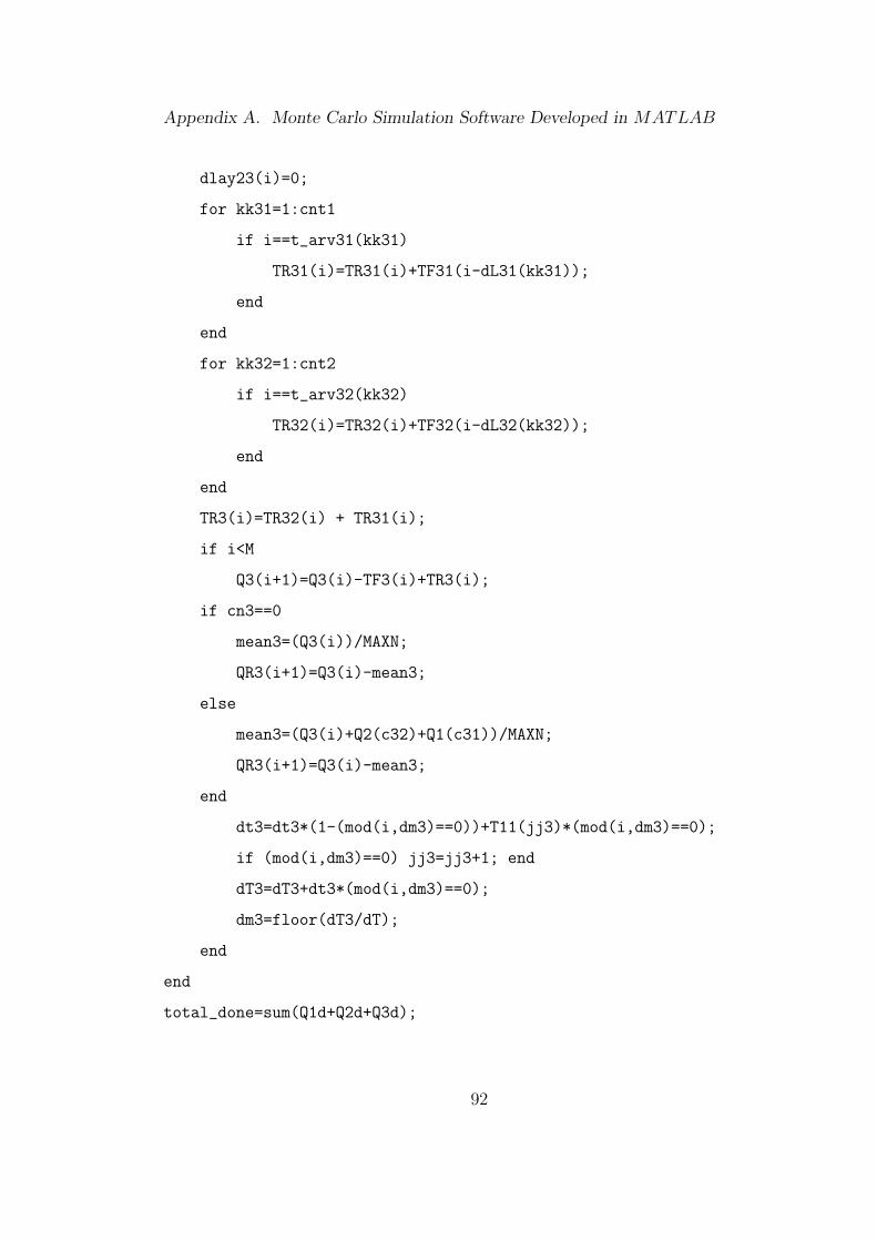
Appendix A. Monte Carlo Simulation Software Developed in MATLAB
dlay23(i)=0;
for kk31=1:cnt1
if i==t_arv31(kk31)
TR31(i)=TR31(i)+TF31(i-dL31(kk31));
end
end
for kk32=1:cnt2
if i==t_arv32(kk32)
TR32(i)=TR32(i)+TF32(i-dL32(kk32));
end
end
TR3(i)=TR32(i) + TR31(i);
if i<M
Q3(i+1)=Q3(i)-TF3(i)+TR3(i);
if cn3==0
mean3=(Q3(i))/MAXN;
QR3(i+1)=Q3(i)-mean3;
else
mean3=(Q3(i)+Q2(c32)+Q1(c31))/MAXN;
QR3(i+1)=Q3(i)-mean3;
end
dt3=dt3*(1-(mod(i,dm3)==0))+T11(jj3)*(mod(i,dm3)==0);
if (mod(i,dm3)==0) jj3=jj3+1; end
dT3=dT3+dt3*(mod(i,dm3)==0);
dm3=floor(dT3/dT);
end
end
total_done=sum(Q1d+Q2d+Q3d);
92

Appendix A. Monte Carlo Simulation Software Developed in MATLAB
%Total completion Time and completion Time for 95% of Tasks.
if (total_done==12000 & flag1==0)
t_full=i;
flag1=1;
end if (total_done >=(0.95*12000) & flag2==0)
t_95=i;
flag2=1;
end
%Queue variance
A(i)=(Q1(i)+Q2(i)+Q3(i))/3; errsum1=errsum1+(abs(A(i)-Q1(i)))^2;
errsum2=errsum2+(abs(A(i)-Q2(i)))^2;
errsum3=errsum3+(abs(A(i)-Q3(i)))^2; end esum1=errsum1/M;
esum2=errsum2/M; esum3=errsum3/M; mserr=(esum1+esum2+esum3)/3;
93

Appendix B
MATLAB Code for Solving
Equations Iteratively
clear all M=500; N=200;
t_b=0; K2_gain=.5; lam_D1=100; lam_D2=100;
lam=lam_D1+lam_D2; if M==0 & N==0
C=0;
elseif M==0 & N>0
if N==1
C=1/lam_D2;
else
[mu]=Initial(M,N,t_b,lam_D1,lam_D2);
C=mu;
end
elseif N==0 & M>0
if M==1
C=1/lam_D1;
else
94

Appendix B. MATLAB Code for Solving Equations Iteratively
%Call the Function which computes
%the initial condition case(m,n):(m,0)
[mu]=Initial(M,N,t_b,lam_D1,lam_D2);
C=mu;
end
else
%%use the following only if (m,n) is not
%%(0,1),(1,0),(m,0),(0,n),(0,0)
T=M+N;
level=0;
C=[1/lam_D2 1/lam_D1];
for i=1:T
k=0;
clear A
level=level+1;
for m=0:level
n=level-m;
if (m<=M & n<=N)
a=[m n];
k=k+1;
A(k)=a(1);
k=k+1;
A(k)=a(2);
end
end
A;
if level~=1
ind=0;
95

Appendix B. MATLAB Code for Solving Equations Iteratively
ptr=1;
ptr_o=0;
while ptr<=k
if A(ptr)==0
ind=ind+1;
m1=A(ptr);
n1=A(ptr+1);
if n1==1
C1(ind)=1/lam_D2;
else
[mu]=Initial(m1,n1,t_b,lam_D1,lam_D2);
%C1(ind)=mu(value brought from the function);
C1(ind)=mu;
end
ptr=ptr+2;
elseif (A(ptr)~=0 & A(ptr+1)~=0)
ind=ind+1;
m1=A(ptr);
n1=A(ptr+1);
ptr_o=ptr_o+1;
%Call the Function which computes
%the initial condition case(m,n):(m,n)
[mu]=Initial_Final(m1,n1);
mult=exp(-lam*t_b);
Kons=lam_D1*C(ptr_o)+lam_D2*C(ptr_o+1)+1;
C1(ind)=mu*mult+Kons*(1-mult)/lam;
%insert formula C1(ind)=with K
%depending on C(ptr_o) and
96

Appendix B. MATLAB Code for Solving Equations Iteratively
%C(ptr_o+1);i.e.
%constant=1+lam1*C(ptr_o)+lam2*C(ptr_o+1)
ptr=ptr+2;
else
ind=ind+1;
m1=A(ptr);
n1=A(ptr+1);
if m1==1
C1(ind)=1/lam_D1;
else
%Call the Function which computes
%the initial condition case(m,n):(m,0)
[mu]=Initial(m1,n1,t_b,lam_D1,lam_D2);
C1(ind)=mu;
end
ptr=ptr+2;
end
end
clear C;
C=C1;
clear C1;
end
end
end
97

References
[1] J. D. Birdwell, T. W. Wang, R. D. Horn, P. Yadav, and D. J. Icove, “Method of
Indexed Storage and Retrieval of Multidimensional Information,”U. S. Patent Appli-
cation, 09/671,304, September 28, 2000.
[2] Z. Lan, V. E. Taylor, and G. Bryan, “Dynamic load balancing for adaptive mesh
refinement application,” in Proc. ICPP’2001, Valencia, Spain, pp. 571-579, 2001.
[3] A.Cortes, A. Ripoll, M.A. Senar and E. Luque, “Performance Comparison of Dynamic
Load-Balancing Strategies for Distributed Computing,” IEEE Proceedings of the 32nd
Hawaii Conference on System Sciences, vol.8, p. 8041, 1999.
[4] D.L. Eager, E.D. Lazowska, and J. Zahorjan, “Adaptive Load Sharing in Homogeneous
Distributed Systems,” IEEE Trans. Software Eng., vol.12, pp. 662–675, no.5, May 1986
[5] J. Liu and V.A. Saletore, “Self-Scheduling on Distributed-Memory Machines,” ACM
Int’l Conf. in Supercomputing,, pp. 814–823, Nov. 1993.
[6] G. Cybenko, “Dynamic load balancing for distributed memory multiprocessors,” IEEE
Trans. Parallel and Distributed Computing, vol. 7, pp. 279–301, Oct. 1989.
[7] K.M. Dragon and J.L. Gustafson, “A Low-Cost Hypercube Load Balance Algorithm,”
Proc. Fourth Conf. Hypercube Concurrent Computers and Applications, pp. 583–590,
1989.
98

References
[8] T.H. Tzen and L.M. Ni, “Dynamic Loop Scheduling for Shared Memory Multiproces-
sors,” Int’l Conf. Parallel Processing, vol. 2, pp. 247–250, 1991.
[9] S. Zhou, “A Trace-Driven Simulation Study of Dynamic Load Balancing,” IEEE Trans.
Software Eng., vol. 14, no. 9, pp. 1,327–1,341, Sept. 1988.
[10] H.G. Rotithor and S.S. Pyo,“Decentralized Decision Making in Adaptive Task Shar-
ing,” Software, vol. 1, no. 3, pp. 66–75, July 1984.
[11] H.C. Lin and C.S. Raghavendra, “A Dynamic Load-Balancing Policy With a Cen-
tral Job Dispatcher (LBC),”IEEE Trans. Software Eng.,vol.18, no.2, pp. 148–158,
Feb.1992.
[12] P. Krueger and M. Livny, “The Diverse Objectives of Distributed Scheduling Policies,”
Proc. Seventh Int’l Conf. Distributed Computing Systems, pp. 242–249, 1987.
[13] B.W. Kernighan and S. Lin, “An Efficient Heuristic Procedure for Partitioning
Graphs,” The Bell System Technical Journal, Vol. 49, pp. 291–307, Feb 1970.
[14] Chi-Chung Hui and Samuel T. Chanson, “Hydrodynamic Load Balancing,” IEEE
Transactions on Parallel and Distributed Systems, vol. 10, No. 11, pp. 1118–1137, Nov.
1999.
[15] Yanyong Zhang, Hubertus Franke, Jose Moreira and Anand Sivasubramaniam, “An
Integrated Approach to Parallel Scheduling Using Gang-Scheduling, Backfilling, and
Migration,” IEEE Transactions on Parallel and Distributed Systems, vol. 14, No. 3,
pp. 236–247, March 2003.
[16] D.A. Bader, B.M.E. Moret, and L. Vawter, “Industrial Applications of High-
Performance Computing for Phylogeny Reconstruction,” SPIE ITCom2001, August
2001. http://www.eece.unm.edu/ dbader/papers/ITCOM2001.pdf.
[17] B.M.E. Moret, D.A. Bader, T. Warnow, “High-Performance Algorithm Engineering
for Computational Phylogenetics,” The Journal of Supercomputing, vol. 22, pp 99–111,
2002.
99

References
[18] S.N.V. Kalluri, J. JaJa , D.A. Bader, Z. Zhang, J.R.G. Townshend, and H. Fallah-Adl.
“ High Performance Computing Algorithms for Land Cover Dynamics Using Remote
Sensing Data,” International Journal of Remote Sensing, vol. 21, No.6 pp. 1513-1536,
2000.
[19] D. A. Bader and J. JaJa. “Practical Parallel Algorithms for Dynamic Data Redistri-
bution, Median Finding, and Selection,” Presented at the 10th International Parallel
Processing Symposium (IPPS 96) Conference, Honolulu, HI, pp. 292-301, April 15-19,
1996.
[20] Michael E. Houle, Antonios Symvonis and David R. Wood, “Dimension-Exchange
Algorithms for Load Balancing on Trees,” Proc. of 9th International Colloquium on
Structural Information and Communication Complexity (SIROCCO ’02), pp. 181–
196, Carleton Scientific, 2002.
[21] Michel Trehel, Chantal Balayer, Abdelghani Alloui, “Modeling Load Balancing
inside Groups using Queuing Theory,” 10th International Conference on Parallel
and Distributed Computing System, New Orleans, Louisiana, Oct1 to Oct. 3, 1997.
http://lifc.univ-fcomte.fr/ trehel/PDCS97.ps
[22] T. L. Casavant and J. G. Kuhl, “A taxonomy of scheduling in general-purpose
distributed computing systems,” IEEE Trans. Software Eng., vol. 14, pp. 141–154,
Feb. 1988.
[23] C. T. Abdallah, N. Alluri, J. D. Birdwell, J. Chiasson, V. Chupryna, Z. Tang, and
T. Wang “A Linear Time Delay Model for Studying Load Balancing Instabilities in
Parallel Computations,” The International Journal of System Science, to appear, 2003.
http://www.eece.unm.edu/faculty/chaouki/journallb.htm
[24] J. D. Birdwell, J. Chiasson, Z. Tang, T. Wang, C. T. Abdallah, and M. M. Hayat, “Dy-
namic Time Delay Models for Load Balancing Part I: Deterministic Models,” CNRS-
NSF Workshop: Advances in Control of Time-Delay Systems, Paris France, Jan. 2003.
100

References
Also, to appear in an edited book by Springer, Kequin Gu and Silviu-Iulian Niculescu,
Editors. /it http://www.lit.net/loadbalanceSIAMextendedAbstract4.pdf
[25] C. T. Abdallah, J.D. Birdwell, J. Chiasson, V. Churpryna, Z. Tang, and T.W. Wang
“Load Balancing Instabilities due to Time Delays in Parallel Computation,” Proceed-
ings of the 3rd IFAC Conference on Time Delay Systems, pp. 198–202, Santa Fe, NM,
Dec. 2001.
[26] M. M. Hayat, S. Dhakal, C. T. Abdallah, J. D. Birdwell, J. Chiasson, “ Dynamic
time delay models for load balancing. Part II: Stochastic analysis of the effect of de-
lay uncertainty,” CNRS-NSF Workshop: Advances in Control of Time-Delay Systems,
Paris France, Jan. 2003. Also, to appear in an edited book by Springer, Kequin Gu
and Silviu-Iulian Niculescu, Editors.
[27] S. Dhakal, B.S. Paskaleva, M.M. Hayat, E. Schamiloglu, C.T. Abdal-
lah “Dynamical Discrete-Time Load Balancing in Distributed Systems in
the Presence of Time Delays,”Accepted for IEEE CDC conf., Dec. 2003.
http://www.ece.unm.edu/faculty/chaouki/paperlb.htm.
[28] J. Ghanem, S. Dhakal, C.T. Abdallah, M.M. Hayat and H. Jerez, “On Load Balancing
in Distributed System with Large Time Delays: Theory and Experiments,” Submitted
to IEEE ACC 2004.
[29] D. J. Daley and D. Vere-Jones, An Introduction to the Theory of Point Processes.
Springer-Verlag, New York, 1988.
[30] C. Knessly and C. Tiery,“Two Tandem queues with general renewal input I: Diffusion
approximation and integral representation,”SIAM J. Appl. Math., vol. 59, pp. 1917–
1959, 1999.
[31] F. Bacelli and P. Bremaud, Elements of Queuing Theory: Palm-Martingale Calculus
and Stochastic Recurrence. New York: Springer-Verlag, 1994.
[32] G. Duffield and W. Whitt, “Control and recovery from rare congestion events in a
large multiserver system,” Queuing Systems, vol. 26, pp. 69-104, 1997.
101

References
[33] T. Kurtz, “Limit theorems for workload input processes. In Stochastic Networks, eds.
F. P. Kelly, S. Zachary and I. Ziedins”, Oxford Publications, Oxford, pp. 119–139, 1997.
[34] S. Shenker, L. Zhang and D.D. Clark, “ Some observations on the dynamics of con-
gestion control algorithm,” Computer Communications Rev., pp. 30–39, 1990.
[35] R. Sandoval-Rodriguez, C.T. Abdallah and P.F. Hokayem,“Internet-like Proto-
cols for the Control and Coordination of Multiple Agents with Time Delay,”
IEEE International Symposium on Intelligent Control, Houston, TX, October 2003.
http://www.eece.unm.edu/controls/papers/cpaper0131.pdf
[36] R. Sandoval-Rodriguez, C.T. Abdallah, P.F. Hokayem and E. Schamiloglu,“Robust
Mobile Robotic Formation Control Using Internet-Like Protocols,” Ac-
cepted for IEEE Conference on Decision and Control, Dec. 2003.
http://www.eece.unm.edu/controls/papers/CDC20031.pdf
102