LLO Calibration for S1 data

Rana Adhikari, Gabriela Gonzalez, Brian O’Reilly

October 5, 2002

Abstract

A summary of calibration information gathered for S1 data.

1 Model used

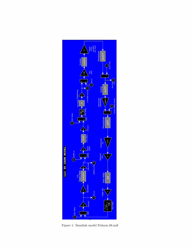
We use a Simulink interferometer model, based on Rana’s “darm 08.mdl”, called “S1darm 08.mdl”, shown inFig1.

The parameters used to load the model are in a file S1darm.m, and are as follow (following the diagram,starting from AS Q)

• Input matrix constant gain asq2darm=0.014 (from conlog).

• LSC Digital Filters

We used “Foton” to translate the numbers in the coefficient filters file (/cvs/cds/llo/chans/L1.txt) usedduring S1, to zeros and poles to use in LTI Matlab models. The filters are digital filters, but we use them inMatlab/Simulink as analog filters (we haven’t yet figured out hot make compatible digital and analog filtersin the linearization programs). This will introduce errors when getting close to the Nyquist frequency, 8kHz.

FM1=zpk([-75.757+i*153.31;-75.757-i*153.31],[0;0],1.99078);

FM2=zpk([-62.8318;-628.241],[-4389.6-i*4389.6;-4389.6+i*4389.6],976.28);

FM3=zpk([],[-8485+i*8485;-8485-i*8485],1.43991e+08);

FM4=zpk([-125.663],[-6.28319],0.996375);

FM8 = zpk([-6207.83;-6207.84],...

[-25045.8+i*0.00338783;-25045.8-i*0.00338783],16.2775);

FM9=zpk([-126.26+i*255.513;-126.26-i*255.513],...

[-12.6263+i*25.552;-12.6263-i*25.552],1.00005);

DARMDF= FM1 * FM2 * FM3 * FM8 * FM9;

• Gain knob: GW K=0.232 (also from conlog). This gain is negative in the LSC code, but we need a negativesign somewhere to make the Simulink loop stable, as the real loop was (this was probably a minus sign insome whitening/dewhitening board).

• Output matrix darm2lm=-0.33 (from output matrix to ETMs, also in conlog).

• ETM filters: there were steep stopbands near the internal modes (near 7 kHz) and a violin mode notch(near 345 Hz) used for the ETM drive. We could not include the stopband filters without running into whatlooked like numerical problems, so since they are outside the gw band, we left them out. Thus, we use justthe violin notch for the test mass filter:

violin = zpk([0+i*2152.47;0-i*2152.47;0+i*2156.2;0-i*2156.2], ...

1

LLO 4K DARM MODEL

4D

AR

M_C

TR

L3

AS

_Q

2C

ontr

olle

r ou

t (V

)

1dL

m O

ut(m

)

−K

−

coun

ts/V

−K

−

Whi

teni

ngG

ain

−K

−

V/C

ount

snub

ber

Snu

bber

2

Sin

gle−

Diff

pdT

F

Pho

todi

ode

pend

TF

Pen

dulu

m

−K

−

Out

put

Mat

rix

opga

in

Opt

ical

Gai

nA

mps

/Met

er

−K

−

N/k

g/A

For

ceco

nsta

ntpe

r m

ass

DA

RM

DF

LmD

igita

l Filt

ers

−K

−

Inpu

tMat

rix

−K

−

Gai

n K

nob

ET

MD

F

ET

M fi

lters

3

Dew

hite

ning

1/2.

8

Dem

od G

ain

V/V

DA

RM

DA

C d

elay

DA

C

arm

TF

Cav

ity

aaf

Ant

i−A

lias

aif

Ant

i Im

age

AD

C d

elay

AD

C

1/30 A/V

(1/R

)

6D

AR

M_i

n

5

Cur

rent

Noi

se (

Am

ps)

4D

AC

Noi

se3

AD

C N

oise

2te

st in

1

dLm

in (

m)

Figure 1: Simulink model S1darm 08.mdl

2

[-10.7623+i*2152.44;-10.7623-i*2152.44;-10.781+i*2156.18; ...

-10.781-i*2156.18],1);

ETMDF=violin;

• DAC gain= (5/32768) Volt/count

• DAC delay: 75µsec. This delay was found to get a good fit to the loop gains.

• Anti-imaging filter: [z,p,k] = ellip(4,4,60,2*pi*7570,’s’); aif = zpk(z,p,k*104/20);

• Dewhitening gain=3

• Voltage to current gain: 1/30 Amp/Volt

• Snubber =0.63 (this factor is fitted to get the measured DC drive of 1.72nm/ct for DARM CTRL, it probablyrepresents the effective gain in the output matrix of the controller)

• Coil/pendulum gain: 0.064/10.3 N/kg/Amp

• Pendulum transfer function (m/N/kg) Q = 10; w0 = 2*pi*0.76; pendTF = 2 * tf(1,[1 w0/Q w02]);

The factor of 2 accounts for Ly-Lx.

• Arm Cavity

fc = 87.3; % Hz

armTF = 2*pi*fc * tf(1,[1 2*pi*fc]);

• Optical gain: 0.47e7 Amps/meter. This gain is multiplied by a fitted factor depending on alignment.

• LSC Photodiode gain: pdTF=400*10 V/Amp.

• Demodulation gain=1/2.8

• Whitening gain: 1018/20

• Anti-Aliasing filter:

[z,p,k] = ellip(8,0.035,80,2*pi*7570,’s’);

aaf = zpk(z,p,k);

• Single-to-differential gain: 2

• ADC delay: 50µsec.

• ADC gain: 32768/10 counts/Volt

The measured DC calibration for DARM CTRL into effective mirror motion (for (Ly-Lx)/2?) was 1.72nm/count.In this model, that gain is made up of the output matrix (0.33), times the DC gain of the ETM filters (1.0), timesthe DAC gain (5/32768 Volts/counts), past the DAC delay (unity gain), the antiimaging filter (unity gain),times the dewhitening gain (3.0), times the voltage-to-current gain (1/30 Amp/Volt), times the force constant(0.064/10.3 N/m/Amp), times the DC pendulum gain (1/w02=0.044 m/N/kg). This product is:

x= 0.33*(5/32768 V/ct)*3*(1/30 A/V)*(0.064/10.3 N/kg/A)*(0.044m/M/kg)*DARM[ct] =2.74 (nm/ct)* DARM[ct]Since the measured value is 1.72nm/count, we use the snubber “fudge factor” of 1.72/2.74=0.63. As mentioned

before, this factor is probably due to the coefficients in the output matrix for the length to each coil drive, whichaverage 85% of the full value (for minimizing length to angle drive at DC).

2 Model and Measurement comparison

We compare the results of this model to the measured swept sine on Sept 06, 2002 at 23:02 UTC, saved indarm loop 020906.xml. We fit a factor to multiply the optical gain so that the loop gains measured and modelledagree.

3

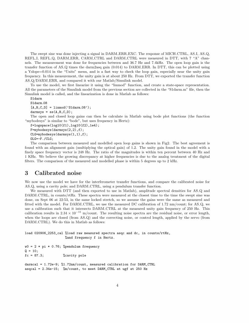
The swept sine was done injecting a signal in DARM ERR EXC. The response of MICH CTRL, AS I, AS Q,REFL I, REFL Q, DARM ERR, CARM CTRL and DARM CTRL were measured in DTT, with 7 “A” chan-nels. The measurement was done for frequencies between and 36.7 Hz and 7.4kHz. The open loop gain is thetransfer function of AS Q times the darm2asq gain (0.014) to DARM ERR. In DTT, this can be plotted usinga Yslope=0.014 in the “Units” menu, and is a fast way to check the loop gain, especially near the unity gainfrequency. In this measurement, the unity gain is at about 250 Hz. From DTT, we exported the transfer functionAS Q/DARM ERR, and compared it with our Matlab/Simulink model.

To use the model, we first linearize it using the “linmod” function, and create a state-space representation.All the parameters of the Simulink model from the previous section are collected in the “S1darm.m” file, then theSimulink model is called, and the linearization is done in Matlab as follows:

S1darm

S1darm 08

[A,B,C,D] = linmod(’S1darm 08’);

darmsys = ss(A,B,C,D);

The open and closed loop gains can then be calculate in Matlab using bode plot functions (the function“mybodesys” is similar to “bode”, but uses frequency in Hertz):

f=logspace(log10(f1),log10(f2),1e4);

F=mybodesys(darmsys(2,2),f);

CLG=mybodesys(darmsys(1,1),f);

OLG=-F./CLG;

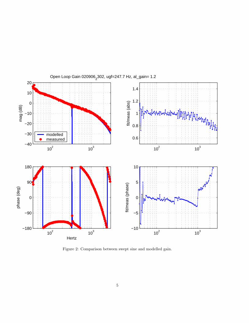
The comparison between measured and modelled open loop gains is shown in Fig2. The best agreement isfound with an alignment gain (multiplying the optical gain) of 1.2. The unity gain found in the model with afinely space frequency vector is 248 Hz. The ratio of the magnitudes is within ten percent between 40 Hz and1 KHz. We believe the growing discrepancy at higher frequencies is due to the analog treatment of the digitalfilters. The comparison of the measured and modelled phase is within 5 degrees up to 2 kHz.

3 Calibrated noise

We now use the model we have for the interferometer transfer functions, and compare the calibrated noise forAS Q, using a cavity pole; and DARM CTRL, using a pendulum transfer function.

We measured with DTT (and then exported to use in Matlab), amplitude spectral densities for AS Q andDARM CTRL, in counts/rtHz. These spectra were measured at the closest time to the time the swept sine wasdone, on Sept 06 at 22:53, in the same locked stretch, so we assume the gains were the same as measured andfitted with the model. For DARM CTRL, we use the measured DC calibration of 1.72 nm/count; for AS Q, weuse a calibration such that it intersects DARM CTRL at the measured unity gain frequency of 250 Hz. Thiscalibration results in 2.34 × 10−15 m/count. The resulting noise spectra are the residual noise, or error length,when the loops are closed (from AS Q) and the correcting noise, or control length, applied by the servo (fromDARM CTRL). We do this in Matlab as follows:

load 020906_2253_cal %load raw measured spectra asqc and dc, in counts/rtHz,

%and frequency f in Hertz.

w0 = 2 * pi * 0.76; %pendulum frequency

Q = 10;

fc = 87.3; %cavity pole

darmcal = 1.72e-9; %1.72nm/count, measured calibration for DARM_CTRL

asqcal = 2.34e-15; %m/count, to meet DARM_CTRL at ugf at 250 Hz

4

102

103

−40

−30

−20

−10

0

10

20

mag

(dB

)

Open Loop Gain 0209062302, ugf=247.7 Hz, al_gain= 1.2

modelledmeasured

102

103

−180

−90

0

90

180

phas

e (d

eg)

Hertz

102

103

0.6

0.8

1

1.2

1.4

fit/m

eas

(abs

)

102

103

−10

−5

0

5

10

fit/m

eas

(pha

se)

Figure 2: Comparison between swept sine and modelled gain.

5

darmtf = darmcal * tf(w0^2,[1 w0/Q w0^2]);

asqtf = asqcal * tf([1 2*pi*fc],[2*pi*fc]);

at = mybodesys(asqtf,f);

dt = mybodesys(darmtf,f);

%noise in m/rtHz

darmn = abs(dt) .* dc;

asqn = abs(at) .* asqc;

We then get a calibration function to use for AS Q from the Simulink model in m/counts, and use it on theloaded spectral density to create a “true” input displacement noise, which for Rana-historical reasons we called“gwp1” in meters/rtHz:

Lmin2asqout=abs(mybodesys(darmsys(3,1),f));

gwp1 = asqc./Lmin2asqout;

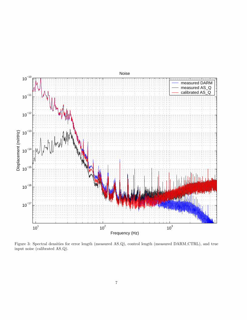
The comparison of the spectra is shown in Fig3. The calibrated spectrum should coincide with DARM CTRLat low frequencies, and with AS Q at high frequencies, and it does!

4 Calibration Lines

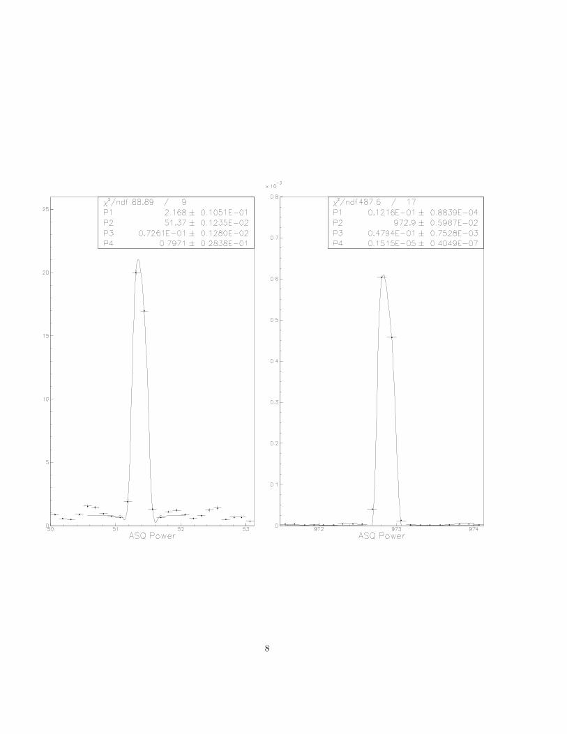
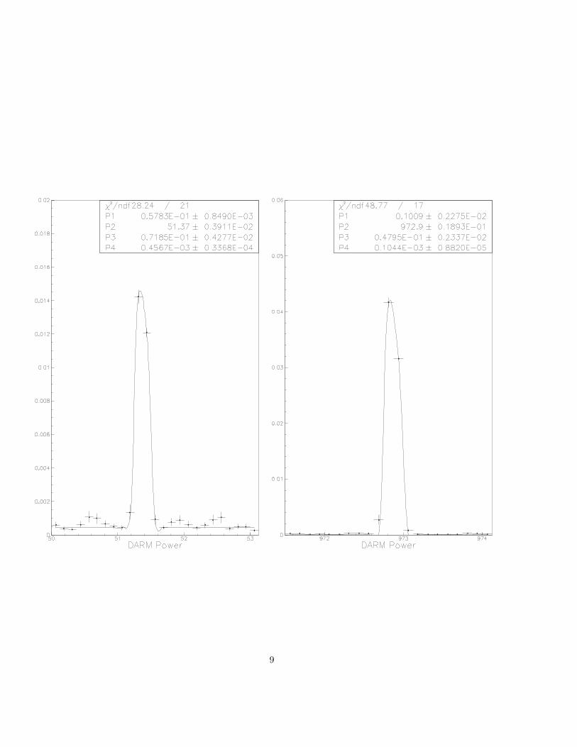
Throughout the run calibration lines were injected in ETMX at 04:28 August 25th UTC (cf. LLO ELOG entryby Giaime). Initially the lines were injected at 37.75Hz and 972.8Hz but the lower line was later moved to 51.3Hzwhich is where it is for this calibration. The change was made at 16:09 Aug. 25th UTC at the suggestion ofRana (cf. LLO ELOG entries around that time), to allow for a smaller line with a large signal to noise ratio (theLLO spectrum has a large value near 35 Hz, so a line with good signal to noise needed to be too large).

The hope is that the power in the lines will track gain changes in the interferometer. Our starting point isthe same amplitude spectral density data described in a previous section. The data are squared so that we canfit the power spectral density (counts2/Hz). We take the error on each point in the PSD ”p” to be ”p/10” sinceit is calculated using 10 averages. When the points lie in the calibration peaks this results in an overestimate ofthe error since we are implicitly assuming Gaussian background noise, which is obviously not true for the injectedsignal. To compensate we use the errors from the adjacent points for the errors on the peak values. This may bea slight underestimate since it does not account for any noise contribution from the injection process.

In Figures 4 and 4 we plot the ASQ and DARM PSD in the region of each calibration line. Each distributionis fit to a Gaussian over a constant background. The parameters returned from the fit are:

• P1 = Counts rms in the peak.

• P2 = Mean frequency of the peak in Hz.

• P3 = Sigma (width) of the peak in Hz.

• P4 = Level of the background in Counts2/Hz.

The fits were performed using the PAW utility from the CERN libraries. It was difficult to get a decent fitand as a consequence the errors on the above quantities should not be taken too seriously. The results obtainedare consistent with a rough estimate made by Gaby. This coupled with the fact that different fits yielded similarresults gives us confidence that the central values are robust.

6

101

102

103

10−17

10−16

10−15

10−14

10−13

10−12

10−11

10−10

Dis

plac

emen

t (m

/rtH

z)

Noise

Frequency (Hz)

measured DARMmeasured AS_Qcalibrated AS_Q

Figure 3: Spectral densities for error length (measured AS Q), control length (measured DARM CTRL), and trueinput noise (calibrated AS Q).

7

8

9

5 Results

Finally, we present a calibration, valid for Sept 06, 22:52 UTC (when a clean locked section started) to 23:02(when the swept sine started). Notice that this is NOT a “science” segment, since calibration procedures werebeing made. However, the alignment and sensitivity during the time of observation for noise spectra were typical.

1. Calibration function Cb(f) for AS Q, in strain/counts.

This is obtained from the Simulink model, for a frequency vector evenly spaced from 0Hz to 2048Hz, with1/64 Hz spacing:

S1darm

S1darm_08

[A,B,C,D] = linmod(’S1darm_08’);

darmsys = ss(A,B,C,D);

fd=[0:1/64:2048];

calib=1./mybodesys(darmsys(3,1),fd);

calib=calib/4e3;

The output is plotted in Figure4, and the frequency triplets (frequency, magnitude and phase) written inthe file ASQCalibration.txt.

2. Sensing function C(f) for AS Q, in strain/counts.

This function is the same calibration function calculated above, except that now the loop is open. Thisfunction involves essentially just the cavity pole transfer function. To keep consistency and include theeffects of the ADC time delay included in the model, we obtain the sensing function with another Simulinkmodel that has the servo links broken. The function is plotted in Figure5, and the frequency triplets writtenin a file ASQSensing.txt

3. Open Loop Gain H(f)

We calculate the open loop gain, again from the Simulink model, that is related to the calibration andsensing functions through Cb(f) = C(f)/(1+H(f)). This function is calculated as the forward loop functiondarmsys(2,2) divided by the closed loop function darmsys(1,1). Since this function has a very large dynamicrange, there are numerical errors visible at low frequencies. We can better estimate the function from themodel by using the analytical expressions known for each block, but for consistency we use the same methodas used when fitting the alignment gain to the loop gains. The (noisy) curve is plotted in Figure6, and thetriplets (always for the same frequency vector) saved in the file OpenLoopGain.txt

4. Amplitudes of calibration lines in AS Q and DARM CTRL.

As described in the previous section, the amplitudes of the calibration lines in AS Q were 2.16± 0.01 countsrms (51.37 Hz) and 0.012 ± 0.001 counts rms (972.9 Hz); and in DARM CTRL, 0.058 ± .001 counts rms(51.37 Hz) and 0.101± .002 counts rms (972.9 Hz).

This output characterizes the calibration of LLO at a given time (09/06/02, 22:50-23:00 UTC). A proceduredescribed elsewhere (?) will be used to propagate this calibration to the rest of S1.

10

10−1

100

101

102

103

10−15

10−10

AS_Q Calibration (Closed Loop)

mag

(str

ain/

coun

t)

10−1

100

101

102

103

−180

−90

0

90

180

angl

e(de

g)

Figure 4: Calibration function for ASQ.

11

10−1

100

101

102

103

10−19

10−18

10−17

10−16

AS_Q Calibration (Open Loop) or Sensing Function

mag

(str

ain/

coun

t

10−1

100

101

102

103

−180

−90

0

90

180

angl

e(de

g)

Figure 5: Calibration function for ASQ.

12

10−1

100

101

102

103

100

105

1010

Open Loop Gain

mag

10−1

100

101

102

103

−180

−90

0

90

180

angl

e(de

g)

Figure 6: Open Loop Gain from S1darm 08.

13

Appendix: List of files

The following files can be found in

http:\\www.phys.lsu.edu\gonzalez\S1Calibration :

• S1calibOct4.tex, *.eps figs called for, and S1calibOct4.pdf: this document.

• Parameters and filters Matlab file: S1darm.m

• Simulink models: S1darm 08.mdl and OpenS1darm.mdl

• Data files:

– Swept Sine: 020906 2302coh.txt (coherence) and 020906 2302.tf.txt (transfer functions). The numbersare for for AS Q/DARM ERR and DARM CTRL/DARM ERR.

– Noise spectra (with calibration lines): 020906 22 53 cal.mat (f,dc,and asqc vectors, for frequency inHertz, DARM CTRL and AS Q in counts/rtHz).

– Calibration results: ASQCalibration.txt; ASQSensing.txt; OpenLoopGain.txt.

• Matlab programs:

– CompareMeasGain.m : Compare meaured gains and modelled gains with Simulink.

– np.m: Plot noise spectral densities of error and control lengths, and calibrated AS Q.

– FinalCalib.m: produces plots and text files mentioned in the previous section about results.

• PAW macros (for calibration lines fits): fit asq.kumac, fit darm.kumac; and FORTRAN fit function gp0.for

14