Live, Runtime Phase Monitoring and Prediction on Real Systemswith Application to Dynamic Power Management

Canturk Isci, Gilberto Contreras and Margaret MartonosiDepartment of Electrical Engineering

Princeton Universitycanturk,gcontrer,mrm@princeton.edu

Abstract

Computer architecture has experienced a major paradigmshift from focusing only on raw performance to consideringpower-performance efficiency as the defining factor of theemerging systems. Along with this shift has come increasedinterest in workload characterization. This interest fuels twoclosely related areas of research. First, various studies explorethe properties of workload variations and develop methods toidentify and track different execution behavior, commonly re-ferred to as “phase analysis”. Second, a large complemen-tary set of research studies dynamic, on-the-fly system man-agement techniques that can adaptively respond to these dif-ferences in application behavior. Both of these lines of workhave produced very interesting and widely useful results. Thusfar, however, there exists only a weak link between these con-ceptually related areas, especially for real-system studies.

Our work aims to strengthen this link by demonstrating areal-system implementation of a runtime phase predictor thatworks cooperatively with on-the-fly dynamic management. Wedescribe a fully-functional deployed system that performs ac-curate phase predictions on running applications. The key in-sight of our approach is to draw from prior branch predictordesigns to create a phase history table that guides predictions.To demonstrate the value of our approach, we implement aprototype system that uses it to guide dynamic voltage and fre-quency scaling. Our runtime phase prediction methodologyachieves above 90% prediction accuracies for many of theexperimented benchmarks. For highly variable applications,our approach can reduce mispredictions by more than 6X overcommonly-used statistical approaches. Dynamic frequencyand voltage scaling, when guided by our runtime phase pre-dictor, achieves energy-delay product improvements as highas 34% for benchmarks with non-negligible variability, on av-erage 7% better than previous methods and 18% better than abaseline unmanaged system.

1 Introduction

The increasing complexity and power demand of proces-sors mandate aggressive dynamic power management tech-niques that can adaptively tune processor execution to theneeds of running applications. These techniques extensivelybenefit from application “phase” information that can pinpointexecution regions with different characteristics. Recognizingthese phases on-the-fly enables various dynamic optimizationssuch as hardware reconfigurations, dynamic voltage and fre-quency scaling (DVFS), thermal management and dynamichotcode optimizations [1, 4, 5, 7, 11, 15, 25, 28].

In recent years, studies have demonstrated different ap-

proaches to track application phase behavior, relying on ex-ecution properties such as control flow [7, 10, 15, 20, 22, 23]or power/performance characteristics [3, 5, 6, 12, 13, 26, 27].While such studies provide useful insights to application be-havior, most of these mainly focus on characterizations ofapplication behavior, summarizing application execution ordetecting repetitive execution phases. Few of these studies[8, 14, 21, 24, 30] also seek to predict future application be-havior. However, to be able to utilize different phase charac-terizations effectively on a running system, there is need fora general dynamic phase prediction framework that can beseamlessly employed on-the-fly during workload execution.Moreover, it is essential to provide a useful, readily-availablebinding between application phase monitoring and prediction,and dynamic, adaptive management opportunities, especiallyon real system implementations.

In this work, we describe a fully-automated, dynamic phaseprediction infrastructure deployed on a running Pentium-Mbased system. We show that a Global Phase History Table(GPHT) predictor, leveraged from a common branch predictortechnique, achieves superior prediction accuracies comparedto other approaches. Our GPHT predictor performs accurateon-the-fly phase predictions for running applications withoutany offline profiling information or any static or dynamic mod-ifications to application execution flow, and with no visibleoverheads.

We demonstrate how our runtime phase predictors can ef-fectively guide dynamic, on-the-fly processor power manage-ment using DVFS as the underlying example dynamic powermanagement technique [9]. Our dynamic phase predictor ef-ficiently cooperates with a DVFS interface to adjust proces-sor execution on-the-fly for improved power/performance ef-ficiency. This GPHT-based dynamic power management canimprove the energy-delay product (EDP) in our deployed ex-perimental system by more than 15%. We also demonstratethat our methodology can be used under different phase def-initions that can be aimed at serving different purposes suchas bounding execution with performance degradation limits.We evaluate our methods on the SPEC2000 benchmark suite,with runtime monitoring using performance monitoring coun-ters (PMCs), and real power measurements with a data acqui-sition (DAQ) unit.

There are three primary contributions of this work. First,we present and evaluate a live, runtime phase predictionmethodology that can seamlessly operate on a real system withno observable overheads. Second, we demonstrate a completereal-system implementation on a deployed system. Our imple-mentation can autonomously function during native operationof the processor, without any profiling or static instrumenta-tion of applications. Nor does it require any underlying virtualmachine or dynamic compilation support. Third, we demon-

strate the application of our phase prediction infrastructure todynamic power management using DVFS as an example tech-nique. Although we present our work with specific phase defi-nitions and power management techniques, our runtime phaseprediction is a general framework. It can be applied to anyfeasible definition of application phases and to other dynamicmanagement techniques, such as dynamic thermal manage-ment or bounding power consumption.

The rest of the paper is organized as follows. Section 2 de-scribes our phase definitions. Section 3 presents our runtimephase prediction methodology and prediction results. Section4 discusses the dependence of phase characterizations to dy-namic management actions. Section 5 describes our prototypereal-system implementation. Section 6 provides our dynamicmanagement results. Section 7 summarizes related work andSection 8 offers our conclusions.

2 Defining PhasesThe key motivation for our work is to develop a phase pre-

diction technique that can be accurately applied at runtime ap-plication execution to guide dynamic power management. Wedescribe and evaluate our proposed prediction technique in de-tail in Section 3. However, first, in this section, we explain ourphase classification methodology, which we also use in theevaluations of Section 3.

The fundamental purpose of phase characterization is toclassify application execution into similar regions of opera-tion. This classification can be done via various features, de-pending on the ease of monitoring and the goal of the appliedphase analysis. Similarly, how the observed features are clas-sified into different phases depends on the target application.

In our work, to track application behavior, we rely on hard-ware performance monitoring counters (PMCs), which canbe configured to monitor execution without disrupting exe-cution flow. For system-level dynamic management, we de-fine relatively coarse grained phases, on the order of millionsof instructions. This guarantees that monitoring of applica-tion behavior—and dynamic management responses—do notlead to any observable overheads. Our phase classifications areconstrained by two factors. First, our experimental platform,described in greater detail in Section 5 supports simultaneousmonitoring of 2 PMCs. Therefore, our classifications of appli-cation behavior can be based on only two configured counters.Second, we monitor PMCs from within a performance mon-itoring interrupt (PMI) routine. Therefore, we need a simpleclassification method to avoid violating interrupt timing con-straints as well as to have negligible performance overheads.In addition, one of the counters has to be dedicated to mon-itor micro-ops (Uops) retired, to trigger the PMI at specifiedinstruction granularities.

We refer to prior work for our choice of monitored PMCevents. Wu et al. [28] make use of event counter informa-tion to assign application routines to different DVFS settingsunder a dynamic instrumentation framework [19]. They de-fine the ratio of memory bus transactions to Uops retired asthe measure of the “memory-boundedness” of an executionregion, and use the ratio of Uops retired to instructions retiredas a proxy to represent available “concurrent execution” in thesame region. These two metrics then determine the available“CPU slack” in the application, which guides different DVFSsettings. For our experiments, we configure the remaining in-

dependent counter to track memory bus transactions. Thus,the ratio of the memory bus transactions to our Uop granu-larity represents the memory-boundedness of each observedphase. We refer to this measure as “Mem/Uop” in the rest ofthe paper.

In addition to Mem/Uop, the two configured counters, to-gether with the time stamp counter (TSC), also enable simulta-neous monitoring of Uops per cycle (UPC), which can provideadditional information on application behavior. These twometrics have already been used cooperatively in other previ-ous studies to guide dynamic power management [27]. How-ever, for phase prediction to perform robustly under dynamicmanagement, our phase classifications have to be resilient tothe effects of dynamic management actions. As we demon-strate in Section 4, while Mem/Uop behavior is virtually in-variant to the responses of our dynamic management tech-nique, UPC can fluctuate strongly. Therefore, for a simple,yet robust phase classification that is largely invariant underdynamic power management, we use Mem/Uop to define ap-plication phases.

We classify Mem/Uop into different phases by observinghow different Mem/Uop rates are assigned to different DVFSsettings in Wu et al.’s description [28]. That work exam-ines memory access rates and concurrency of different appli-cations on a similar experimental platform. Then, it calcu-lates the DVFS settings for different application regions basedon a performance loss formulation. For our phase defini-tions, we convert these statistics to Mem/Uop rates and avail-able concurrency ranges for each DVFS setting. As we donot have the concurrency measure available for our runtimemonitoring and prediction, we base our phase classificationsto the derived Mem/Uop ranges for the common lowest ob-served concurrency—i.e. Uops retired/instructions retired ≈1. Based on this classification, we define 6 phase categoriesas shown in Table 1. Conceptually, category 1 correspondsto a highly CPU-bound execution pattern that should be runas fast as possible, and category 6 corresponds to a highlymemory-bound phase, where the application can be signifi-cantly slowed down to exploit available slack.

Mem/Uop Phase #

< 0.005 1 (highly cpu-bound)

[0.005,0.010) 2

[0.010,0.015) 3

[0.015,0.020) 4

[0.020,0.030) 5

> 0.030 6 (highly memory-bound)

Table 1. Definition of phases based on Mem/Uoprates.

3 Predicting Phases with a Global Phase His-tory Table Predictor

In this section, we first discuss different prediction optionsand describe our chosen technique. Afterwards, we presentour phase prediction evaluations. For a phase prediction tech-nique that can perform well on all corners of benchmark be-havior, we propose a Global Phase History Table (GPHT) pre-dictor. There exist other prior history based predictors that

also target at estimating application performance characteris-tics [8, 14]. However, predictors that simply rely on the statis-tics of past behavior cannot perform well for highly variablebenchmarks. To demonstrate this comparatively, we also con-sider some of the simple statistical predictors in our evalua-tions.

The simplest statistical predictor is the last value predic-tor. In this predictor, the next sample behavior of an appli-cation is assumed to be identical to its last seen behavior.In this case, predicted phase in the next interval can be ex-pressed as Phase[t + 1] = Phase[t]. This can be extended toencompass longer past histories by considering a fixed historywindow predictor, where the predictions are based on the lastwindow size observations. In this case, the next phase pre-diction can be phrased as Phase[t +1] = f (Phase[t],Phase[t−1], ...,Phase[t−(winsize−1)]). The function f () can be a sim-ple averaging function, an exponential moving average or a se-lector, based on population counts. Another approach, similarto fixed history window is a variable history window predictor.In this case, the history can be shrunk in case of a phase transi-tion, where previous history becomes obsolete for the follow-ing phase predictions.

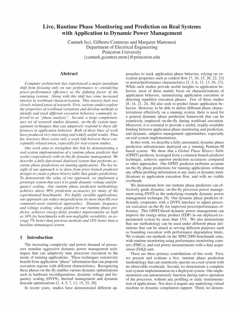
In contrast, our Global Phase History Table (GPHT) pre-dictor observes the patterns from previous samples to deducethe next phase behavior. In such an approach, it relies on thewidely acknowledged repetitive execution behavior of appli-cations. Structurally, the GPHT predictor, depicted in Figure1, is similar to a global branch history predictor [29]. Unlikehardware branch predictors, however, the GPHT is a softwaretechnique, implemented in the operating system for high-level,dynamic phase prediction.

Pt Pt-1 Pt-2 … … Pt-N … … Pt’’ Pt’’-1 Pt’’-2 … … Pt’’-N … …

Pt’ Pt’-1 Pt’-2 … … Pt’-N … …

: : : : : : : :

: : : : : : : :

: : : : : : : :

P0 P0 P0 … … P0 … …

Pt’’+1

Pt’+1

:

:

:

P0

15

20

:

:

:

-1

Pt

Last observed phase from performance counters

GPHR

PHT PHT Tags PHT Pred-n

Age / Invalid

GPHR depth

GPHR depth

PH

T entries

Figure 1. GPHT predictor structure.

Similar to a global branch predictor, a GPHT predictor con-sists of a global shift register, called the Global Phase HistoryRegister (GPHR), that tracks the last few observed phases. Thelength of the history is specified by GPHR depth. At each sam-pling period, the GPHR is updated with the last seen phase, asobserved from PMCs. This updated GPHR content is used toindex a Pattern History Table (PHT). The PHT holds severalpreviously observed phase patterns, with their corresponding“next phase” predictions based on previous experience. Thesephase predictions are shown as the PHT Pred-n vector in thePHT. The GPHR index is associatively compared to the storedvalid PHT tags, and if a match is found, the correspondingPHT prediction is used as the final prediction. An Age / In-valid entry is kept for each tag to track the ages of differentPHT tags for a least recently used (LRU) replacement policywhen the PHT is full. A −1 entry denotes the correspondingtag contents and prediction are not valid. The number of en-tries in the PHT is specified by PHT entries. In the case of

a mismatch between GPHR and PHT tags, the last observedphase, stored in GPHR[0], is predicted as the next phase. Af-ter a mismatch, the current GPHR contents are added to thePHT by either replacing the oldest entry or by occupying anavailable invalid entry. In the case of a match, a PHT predic-tion entry is updated in the next sampling period based on theactual observed phase for the corresponding tag.

By observing the phase patterns in application execution,the GPHT predictor can perform reliable predictions even forhighly variable benchmarks. Inevitably, for a hypothetical ap-plication with no evident recurrent behavior, no predictor canperform good predictions. In such cases there is no match-ing pattern in PHT and we revert to a last value predictor,thus guaranteeing to meet the accuracy of previous methodsunder worst case scenarios. Most applications exhibit someamount of repetitive patterns, however, due to the commonloop-oriented and procedural execution style.

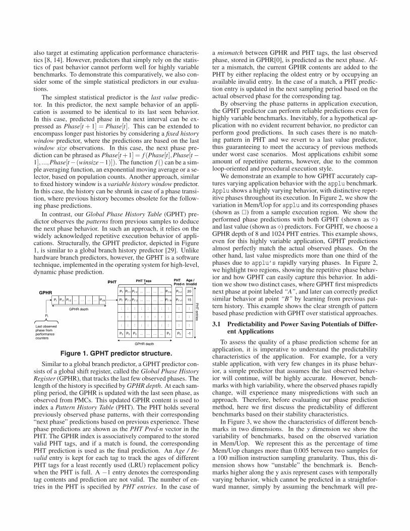
We demonstrate an example to how GPHT accurately cap-tures varying application behavior with the applu benchmark.Applu shows a highly varying behavior, with distinctive repet-itive phases throughout its execution. In Figure 2, we show thevariation in Mem/Uop for applu and its corresponding phases(shown as ) from a sample execution region. We show theperformed phase predictions with both GPHT (shown as )and last value (shown as ) predictors. For GPHT, we choose aGPHR depth of 8 and 1024 PHT entries. This example shows,even for this highly variable application, GPHT predictionsalmost perfectly match the actual observed phases. On theother hand, last value mispredicts more than one third of thephases due to applu’s rapidly varying phases. In Figure 2,we highlight two regions, showing the repetitive phase behav-ior and how GPHT can easily capture this behavior. In addi-tion we show two distinct cases, where GPHT first mispredictsnext phase at point labeled “A”, and later can correctly predictsimilar behavior at point “B” by learning from previous pat-tern history. This example shows the clear strength of patternbased phase prediction with GPHT over statistical approaches.

3.1 Predictability and Power Saving Potentials of Differ-ent Applications

To assess the quality of a phase prediction scheme for anapplication, it is imperative to understand the predictabilitycharacteristics of the application. For example, for a verystable application, with very few changes in its phase behav-ior, a simple predictor that assumes the last observed behav-ior will continue, will be highly accurate. However, bench-marks with high variability, where the observed phases rapidlychange, will experience many mispredictions with such anapproach. Therefore, before evaluating our phase predictionmethod, here we first discuss the predictability of differentbenchmarks based on their stability characteristics.

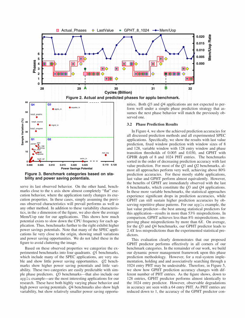
In Figure 3, we show the characteristics of different bench-marks in two dimensions. In the y dimension we show thevariability of benchmarks, based on the observed variationin Mem/Uop. We represent this as the percentage of timeMem/Uop changes more than 0.005 between two samples fora 100 million instruction sampling granularity. Thus, this di-mension shows how “unstable” the benchmark is. Bench-marks higher along the y axis represent cases with temporallyvarying behavior, which cannot be predicted in a straightfor-ward manner, simply by assuming the benchmark will pre-

0

1

2

3

4

5

6

7

8

9

10

28 29 30 31 32Cycles (Billion)

Ph

ases

-0.015

-0.010

-0.005

0.000

0.005

0.010

0.015

0.020

Mem

/Uo

p R

ate

Actual_Phases LastValue GPHT_8_1024 Mem/Uop

A B

Figure 2. Actual and predicted phases for applu benchmark.

applu_inequake_in

ammp

apsi

bzip2_graphic

bzip2_program

bzip2_source

gap

gcc_166

gcc_expr

mgrid_in

parser

swim_intwolf_ref

wupwise

0

10

20

30

40

50

60

0.000 0.005 0.010 0.015 0.020 0.025 0.030

Power Savings Potential

Sam

ple

Var

iati

on

(%

)

0.100 0.110 0.120

mcf_inp

Q4

Q1 Q2

Q3

Figure 3. Benchmark categories based on sta-bility and power saving potentials.

serve its last observed behavior. On the other hand, bench-marks close to the x axis show almost completely “flat” exe-cution behavior, where the application rarely changes its exe-cution properties. In these cases, simply assuming the previ-ous observed characteristics will prevail performs as well asany other method. In addition to these variability characteris-tics, in the x dimension of the figure, we also show the averageMem/Uop rate for our applications. This shows how muchpotential exists to slow down the CPU frequency for each ap-plication. Thus, benchmarks further to the right exhibit higherpower savings potentials. Note that many of the SPEC appli-cations lie very close to the origin, showing small variationsand power saving opportunities. We do not label these in thefigure to avoid cluttering the image.

Based on these observed properties we categorize the ex-perimented benchmarks into four quadrants. Q1 benchmarks,which include many of the SPEC applications, are very sta-ble and show little power saving opportunities. Q2 bench-marks show higher power saving potentials and little vari-ability. These two categories are easily predictable with sim-ple phase predictors. Q3 benchmarks—that also include ourapplu example—are the most interesting applications for ourresearch. These have both highly varying phase behavior andhigh power saving potentials. Q4 benchmarks also show highvariability, but show relatively smaller power saving opportu-

nities. Both Q3 and Q4 applications are not expected to per-form well under a simple phase prediction strategy that as-sumes the next phase behavior will match the previously ob-served one.

3.2 Phase Prediction Results

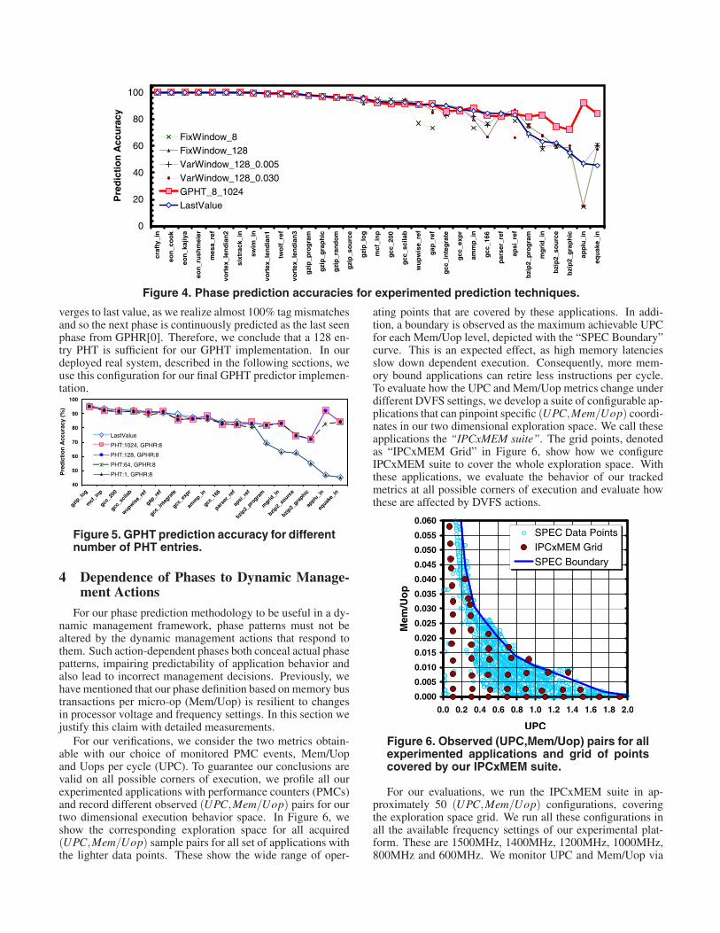
In Figure 4, we show the achieved prediction accuracies forall discussed prediction methods and all experimented SPECapplications. Specifically, we show the results with last valueprediction, fixed window prediction with window sizes of 8and 128, variable window with 128 entry window and phasetransition thresholds of 0.005 and 0.030, and GPHT withGPHR depth of 8 and 1024 PHT entries. The benchmarkssorted in the order of decreasing prediction accuracy with lastvalue prediction. For most of the Q1 and Q2 benchmarks, al-most all approaches perform very well, achieving above 80%prediction accuracies. For these mostly stable applications,last value and GPHT perform almost equivalently. However,the benefits of GPHT are immediately observed with the last6 benchmarks, which constitute the Q3 and Q4 applications.In these more variable benchmarks, the statistical approachesexperience significant drops in prediction accuracies, whileGPHT can still sustain higher prediction accuracies by ob-serving repetitive phase patterns. For our applu example, thelast value predictor—the best among statistical predictors forthis application—results in more than 53% mispredictions. Incomparison, GPHT achieves less than 8% mispredictions, im-proving phase mispredictions by more than 6X . On average,for the Q3 and Q4 benchmarks, our GPHT predictor leads to2.4X less mispredictions than the experimented statistical pre-dictors.

This evaluation clearly demonstrates that our proposedGPHT predictor performs effectively in all corners of ourbenchmark categories. In the remainder of our work, we buildour dynamic power management framework upon this phaseprediction methodology. However, for a real-system imple-mentation, holding and and associatively searching through a1024 entry PHT may be undesirable. Therefore, in Figure 5,we show how GPHT prediction accuracy changes with dif-ferent number of PHT entries. As the figure shows, down to128 entries, GPHT predictor performs almost identically tothe 1024 entry predictor. However, observable degradationsin accuracy are seen with a 64 entry PHT. As PHT entries arereduced down to 1, the accuracy of the GPHT predictor con-

0

20

40

60

80

100

craf

ty_i

n

eon

_co

ok

eon

_kaj

iya

eon

_ru

shm

eier

mes

a_re

f

vort

ex_l

end

ian

2

sixt

rack

_in

swim

_in

vort

ex_l

end

ian

1

two

lf_r

ef

vort

ex_l

end

ian

3

gzi

p_p

rog

ram

gzi

p_g

rap

hic

gzi

p_r

and

om

gzi

p_s

ou

rce

gzi

p_l

og

mcf

_in

p

gcc

_200

gcc

_sci

lab

wu

pw

ise_

ref

gap

_ref

gcc

_in

teg

rate

gcc

_exp

r

amm

p_i

n

gcc

_166

par

ser_

ref

apsi

_ref

bzi

p2_

pro

gra

m

mg

rid

_in

bzi

p2_

sou

rce

bzi

p2_

gra

ph

ic

app

lu_i

n

equ

ake_

in

Pre

dic

tio

n A

ccu

racy

FixWindow_8FixWindow_128VarWindow_128_0.005VarWindow_128_0.030GPHT_8_1024LastValue

Figure 4. Phase prediction accuracies for experimented prediction techniques.

verges to last value, as we realize almost 100% tag mismatchesand so the next phase is continuously predicted as the last seenphase from GPHR[0]. Therefore, we conclude that a 128 en-try PHT is sufficient for our GPHT implementation. In ourdeployed real system, described in the following sections, weuse this configuration for our final GPHT predictor implemen-tation.

40

50

60

70

80

90

100

gzip_lo

g

mcf

_inp

gcc_2

00

gcc_s

cilab

wupwise_r

ef

gap_r

ef

gcc_in

tegra

te

gcc_e

xpr

amm

p_in

gcc_1

66

parse

r_re

f

apsi_

ref

bzip2_

progra

m

mgrid

_in

bzip2_

sourc

e

bzip2_

graphic

applu

_in

equak

e_in

Pre

dic

tio

n A

ccu

racy

(%

)

LastValue

PHT:1024, GPHR:8

PHT:128, GPHR:8

PHT:64, GPHR:8

PHT:1, GPHR:8

Figure 5. GPHT prediction accuracy for differentnumber of PHT entries.

4 Dependence of Phases to Dynamic Manage-ment Actions

For our phase prediction methodology to be useful in a dy-namic management framework, phase patterns must not bealtered by the dynamic management actions that respond tothem. Such action-dependent phases both conceal actual phasepatterns, impairing predictability of application behavior andalso lead to incorrect management decisions. Previously, wehave mentioned that our phase definition based on memory bustransactions per micro-op (Mem/Uop) is resilient to changesin processor voltage and frequency settings. In this section wejustify this claim with detailed measurements.

For our verifications, we consider the two metrics obtain-able with our choice of monitored PMC events, Mem/Uopand Uops per cycle (UPC). To guarantee our conclusions arevalid on all possible corners of execution, we profile all ourexperimented applications with performance counters (PMCs)and record different observed (UPC,Mem/Uop) pairs for ourtwo dimensional execution behavior space. In Figure 6, weshow the corresponding exploration space for all acquired(UPC,Mem/Uop) sample pairs for all set of applications withthe lighter data points. These show the wide range of oper-

ating points that are covered by these applications. In addi-tion, a boundary is observed as the maximum achievable UPCfor each Mem/Uop level, depicted with the “SPEC Boundary”curve. This is an expected effect, as high memory latenciesslow down dependent execution. Consequently, more mem-ory bound applications can retire less instructions per cycle.To evaluate how the UPC and Mem/Uop metrics change underdifferent DVFS settings, we develop a suite of configurable ap-plications that can pinpoint specific (UPC,Mem/Uop) coordi-nates in our two dimensional exploration space. We call theseapplications the “IPCxMEM suite”. The grid points, denotedas “IPCxMEM Grid” in Figure 6, show how we configureIPCxMEM suite to cover the whole exploration space. Withthese applications, we evaluate the behavior of our trackedmetrics at all possible corners of execution and evaluate howthese are affected by DVFS actions.

0.000

0.005

0.010

0.015

0.020

0.025

0.030

0.035

0.040

0.045

0.050

0.055

0.060

0.0 0.2 0.4 0.6 0.8 1.0 1.2 1.4 1.6 1.8 2.0

UPC

Mem

/Uo

p

SPEC Data PointsIPCxMEM Grid

SPEC Boundary

Figure 6. Observed (UPC,Mem/Uop) pairs for allexperimented applications and grid of pointscovered by our IPCxMEM suite.

For our evaluations, we run the IPCxMEM suite in ap-proximately 50 (UPC,Mem/Uop) configurations, coveringthe exploration space grid. We run all these configurations inall the available frequency settings of our experimental plat-form. These are 1500MHz, 1400MHz, 1200MHz, 1000MHz,800MHz and 600MHz. We monitor UPC and Mem/Uop via

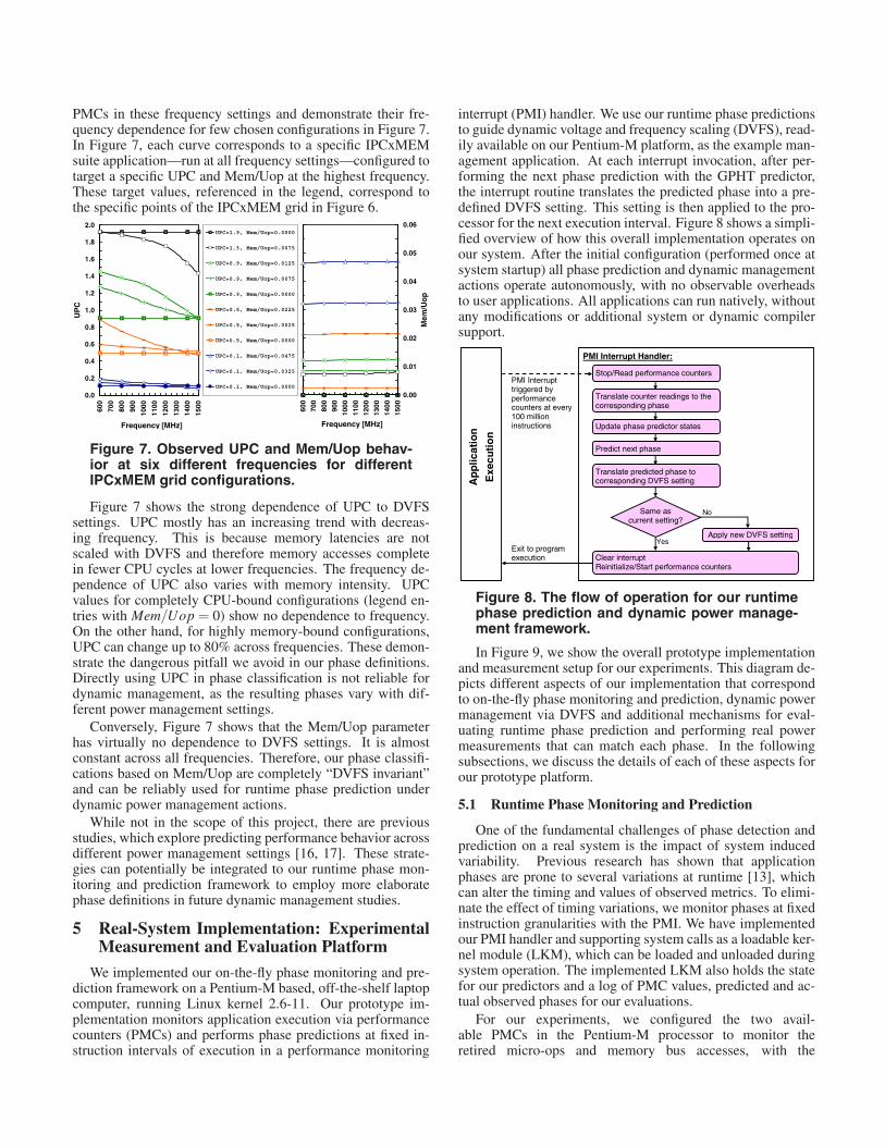
PMCs in these frequency settings and demonstrate their fre-quency dependence for few chosen configurations in Figure 7.In Figure 7, each curve corresponds to a specific IPCxMEMsuite application—run at all frequency settings—configured totarget a specific UPC and Mem/Uop at the highest frequency.These target values, referenced in the legend, correspond tothe specific points of the IPCxMEM grid in Figure 6.

600

700

800

900

1000

1100

1200

1300

1400

1500

Frequency [MHz]

0.00

0.01

0.02

0.03

0.04

0.05

0.06

Mem

/Uo

p

0.0

0.2

0.4

0.6

0.8

1.0

1.2

1.4

1.6

1.8

2.0

600

700

800

900

1000

1100

1200

1300

1400

1500

Frequency [MHz]

UP

C

UPC=1.9, Mem/Uop=0.0000

UPC=1.3, Mem/Uop=0.0075

UPC=0.9, Mem/Uop=0.0125

UPC=0.9, Mem/Uop=0.0075

UPC=0.9, Mem/Uop=0.0000

UPC=0.5, Mem/Uop=0.0225

UPC=0.5, Mem/Uop=0.0025

UPC=0.5, Mem/Uop=0.0000

UPC=0.1, Mem/Uop=0.0475

UPC=0.1, Mem/Uop=0.0325

UPC=0.1, Mem/Uop=0.0000

Figure 7. Observed UPC and Mem/Uop behav-ior at six different frequencies for differentIPCxMEM grid configurations.

Figure 7 shows the strong dependence of UPC to DVFSsettings. UPC mostly has an increasing trend with decreas-ing frequency. This is because memory latencies are notscaled with DVFS and therefore memory accesses completein fewer CPU cycles at lower frequencies. The frequency de-pendence of UPC also varies with memory intensity. UPCvalues for completely CPU-bound configurations (legend en-tries with Mem/Uop = 0) show no dependence to frequency.On the other hand, for highly memory-bound configurations,UPC can change up to 80% across frequencies. These demon-strate the dangerous pitfall we avoid in our phase definitions.Directly using UPC in phase classification is not reliable fordynamic management, as the resulting phases vary with dif-ferent power management settings.

Conversely, Figure 7 shows that the Mem/Uop parameterhas virtually no dependence to DVFS settings. It is almostconstant across all frequencies. Therefore, our phase classifi-cations based on Mem/Uop are completely “DVFS invariant”and can be reliably used for runtime phase prediction underdynamic power management actions.

While not in the scope of this project, there are previousstudies, which explore predicting performance behavior acrossdifferent power management settings [16, 17]. These strate-gies can potentially be integrated to our runtime phase mon-itoring and prediction framework to employ more elaboratephase definitions in future dynamic management studies.

5 Real-System Implementation: ExperimentalMeasurement and Evaluation Platform

We implemented our on-the-fly phase monitoring and pre-diction framework on a Pentium-M based, off-the-shelf laptopcomputer, running Linux kernel 2.6-11. Our prototype im-plementation monitors application execution via performancecounters (PMCs) and performs phase predictions at fixed in-struction intervals of execution in a performance monitoring

interrupt (PMI) handler. We use our runtime phase predictionsto guide dynamic voltage and frequency scaling (DVFS), read-ily available on our Pentium-M platform, as the example man-agement application. At each interrupt invocation, after per-forming the next phase prediction with the GPHT predictor,the interrupt routine translates the predicted phase into a pre-defined DVFS setting. This setting is then applied to the pro-cessor for the next execution interval. Figure 8 shows a simpli-fied overview of how this overall implementation operates onour system. After the initial configuration (performed once atsystem startup) all phase prediction and dynamic managementactions operate autonomously, with no observable overheadsto user applications. All applications can run natively, withoutany modifications or additional system or dynamic compilersupport.

Ap

plic

atio

n

Exe

cuti

on

PMI Interrupt Handler:

Stop/Read performance counters

Translate counter readings to the corresponding phase

Update phase predictor states

Predict next phase

Translate predicted phase to corresponding DVFS setting

Same as current setting?

Apply new DVFS setting

Clear interrupt Reinitialize/Start performance counters

No

Yes

PMI Interrupt triggered by performance counters at every 100 million instructions

Exit to program execution

Figure 8. The flow of operation for our runtimephase prediction and dynamic power manage-ment framework.

In Figure 9, we show the overall prototype implementationand measurement setup for our experiments. This diagram de-picts different aspects of our implementation that correspondto on-the-fly phase monitoring and prediction, dynamic powermanagement via DVFS and additional mechanisms for eval-uating runtime phase prediction and performing real powermeasurements that can match each phase. In the followingsubsections, we discuss the details of each of these aspects forour prototype platform.

5.1 Runtime Phase Monitoring and Prediction

One of the fundamental challenges of phase detection andprediction on a real system is the impact of system inducedvariability. Previous research has shown that applicationphases are prone to several variations at runtime [13], whichcan alter the timing and values of observed metrics. To elimi-nate the effect of timing variations, we monitor phases at fixedinstruction granularities with the PMI. We have implementedour PMI handler and supporting system calls as a loadable ker-nel module (LKM), which can be loaded and unloaded duringsystem operation. The implemented LKM also holds the statefor our predictors and a log of PMC values, predicted and ac-tual observed phases for our evaluations.

For our experiments, we configured the two avail-able PMCs in the Pentium-M processor to monitor theretired micro-ops and memory bus accesses, with the

Pentium-M Processor

Performance counters

DVFS mode set registers

Predictor state

PMC and phase log

OS kernel

PMI Interrupt

Stop/Read Counters

Initialize/Start Counters

Check DVFS mode

Set DVFS mode

Power supply

Voltage regulator

V2

V1

I2

R2=2mΩ

I1

R1=2mΩ VCPU

Prototype Machine

Par

alle

l po

rt

PMI Interrupt handler 1

2

3

Sig

nal

co

nd

itio

nin

g u

nit

and

Dat

a A

cqu

isit

ion

Sys

tem

Bits 0-2

VCPU

V2

V1

Bits 0-2

VCPU

I2

I1

Logging

Machine

Real Power Measurement Units

Figure 9. Developed measurement and evaluation platform. Regions identified as 1, 2 and 3 via dashedlines correspond to different parts of implementation relevant to on-the-fly phase monitoring and pre-diction(1), dynamic management with DVFS(2) and measurement and evaluation support(3).

UOPS_RETIRED and BUS_TRAN_MEM event configura-tions. We have experimented with various instruction granu-larities and used 100 million instructions as a safe granularityto invoke our interrupt handler. Therefore, after each invoca-tion, the first PMC is reinitialized to overflow after 100 millionretired Uops.

After each 100 million instructions, the interrupt handlerstops and reads the PMCs, updates the GPHT predictor statesand performs the next phase prediction. It also logs the ob-served PMC values, actual observed phase for the past periodand the predicted phase for the next period for our evaluations.At its exit, the handler clears the PMC overflow bit, reinitial-izes the PMCs and time stamp counter (TSC) and restarts thecounters.

5.2 Dynamic Power Management via DVFS

Our on-the-fly phase prediction methodology can be uti-lized to guide a range of dynamic management techniques.In this work we consider DVFS as an example implementa-tion, which is supported on our platform via Intel SpeedSteptechnology [9]. In our prototype implementation, we use alook-up table, defined at LKM initialization, to quickly trans-late the predicted phase to one of the 6 DVFS settings withinthe handler. For our prototype machine and our original phasedefinitions, these are shown in Table 2. For alternative phasedefinitions or management schemes, we can simply reconfig-ure this table. At each sampling interval, the handler translatesthe predicted phase to the corresponding DVFS setting. Thenit compares this to the current setting and updates the DVFSmode set registers if necessary. Our 100 million instructiongranularity (on the order of 100 ms) guarantees that the over-heads induced by interrupt handling and DVFS application (onthe order of 10-100 µs) are essentially invisible to native ap-plication execution.

5.3 Power Measurement

To track the power consumed by the Pentium-M proces-sor, we measure the input voltage and current flow to the pro-cessor. For this purpose, we use an external data acquisition

Mem/Uop Phase # DVFS Setting

< 0.005 1 (1500 MHz, 1484 mV)

[0.005,0.010) 2 (1400 MHz, 1452 mV)

[0.010,0.015) 3 (1200 MHz, 1356 mV)

[0.015,0.020) 4 (1000 MHz, 1228 mV)

[0.020,0.030) 5 ( 800 MHz, 1116 mV)

> 0.030 6 ( 600 MHz, 956 mV)

Table 2. Translation of phases to DVFS settings.

system (DAQ) that is connected to the processor board. Ourlaptop board includes two 2 mΩ precision sense resistors thatreside between the voltage regulator module and the Pentium-M CPU, shown as R1 and R2 in Figure 9. The total currentthat flows through these resistors represents the current flowinto the CPU. The voltage after the resistors, denoted as VCPU ,represents the input voltage of the CPU.

In the actual measurement setup, we measure the three volt-ages V1, V2 and VCPU , to track processor current and volt-age. These voltages—and additional parallel port bits forevaluation support—are first fed into a National InstrumentsAI05 Signal Conditioning Unit. This unit filters the noise onthe measured voltage signals and calculates the voltage dropacross the two resistors. These voltage drops, (V1 −VCPU ) and(V2 −VCPU ) and the CPU voltage VCPU are then fed into a Na-tional Instruments DAQPad 6070E Data Acquisition System.This unit then scales the voltage drops with the resistor val-ues to compute the current flows as I1 = (V1 −VCPU )/0.002and I2 = (V2 −VCPU )/0.002. The DAQ system monitors a to-tal of eight signals, and has a sampling period of 40 µs. Thetwo measured currents and CPU voltage, together with addi-tional parallel port signals are sent to a separate logging ma-chine, which logs the observed currents and voltages. TheCPU power consumption for each sample is computed on thislogging machine as PowerCPU = VCPU · (I1 + I2). With thiscomplete measurement setup, we can accurately track CPUpower consumption. By also utilizing parallel port signal-ing, described below, our measurement setup can individually

compute the power consumption and performance statistics foreach 100M-instruction phase sample, as well as for the wholeexecution of applications.

5.4 Evaluation Support

The overall correct operation of our developed system re-quires only on-the-fly phase monitoring and prediction, anddynamic power management with DVFS as highlighted in re-gions 1 and 2 in Figure 9. However, for experimental evalu-ation of phase prediction and dynamic management methods,we develop additional components on our prototype system.First, we use the above described real power measurementsetup to measure processor power consumption. In addition,for detailed power/performance and phase prediction evalua-tions, we employ additional mechanisms in our implementa-tion; these fall into region 3 in Figure 9.

To evaluate runtime phase prediction accuracy and to ana-lyze application behavior, we use a separate kernel log in ourLKM. This log keeps track of the actual observed and pre-dicted phases for each sample as well as memory accesses perUop and Uops per cycle for each phase. At each invocation,the handler logs relevant information in this log. Afterwards, auser-level tool can access this information via separate systemcalls.

The execution of the processor—under our runtime phaseprediction and dynamic management—and the real powermeasurements are inherently two completely independent pro-cesses. To provide a synchronizing link between the two sidesof our framework, we use parallel port bits that signal specificprocessor execution information to the DAQ system. We usethree parallel port bits. Bit 2 is set from the user level via sys-tem calls at the start of an application execution and is clearedwhen an application ends. This helps DAQ to measure powerspecifically during an application execution. Bit 1 is used todistinguish between application and interrupt execution. Thisbit is set by the handler at the entrance to the handler rou-tine and is cleared at exit. Finally, bit 0 is used to help theDAQ track each phase. The handler flips this bit at each sam-pling interval so that the DAQ and the logging machine candistinguish each phase and compute power and performancestatistics individually for each phase.

In Figure 10, we show a detailed view of the overall op-eration of our deployed system with the applu benchmark,performing on-the-fly phase predictions with the GPHT pre-dictor and dynamic power management with DVFS. The fig-ure shows the measured prediction, power and performanceresults with respect to a baseline, unmanaged system. Inthe top chart, we first show the observed Mem/Uop behav-ior for the two runs of applu, with and without our describedtechniques. The two curves are almost identical between thetwo real-system runs, which shows (i) our phases, defined byMem/Uop, are DVFS invariant and can be safely used forphase prediction under dynamic management responses; and(ii) our fixed instruction granularity phase definitions are re-silient to real-system variations. In the lower part of the topchart, we show the actual and predicted phases with the GPHT.Once again, the GPHT exhibits very good prediction accura-cies for such a highly varying application. The middle chartshows the power measured for each phase during applu ex-ecution for both systems, where the shaded area between thetwo curves demonstrates power savings achieved with our ap-

0

1

2

3

4

5

6

7

8

9

10

1.5E+09 2.5E+09 3.5E+09 4.5E+09

Instructions

Ph

ases

-0.016

-0.012

-0.008

-0.004

0.000

0.004

0.008

0.012

0.016

0.020

0.024

Mem

/Uo

p

ACTUAL_PHASE PRED_PHASE (GPHT) Mem/Uop (Baseline) Mem/Uop (GPHT)

0

2

4

6

8

10

12

14

1.5E+09 2.5E+09 3.5E+09 4.5E+09

Instructions

Po

wer

[W

]

Power (Baseline) Power (GPHT)

0

0.3

0.6

0.9

1.2

1.5

1.8

2.1

1.5E+09 2.0E+09 2.5E+09 3.0E+09 3.5E+09 4.0E+09 4.5E+09 5.0E+09

Instructions

BIP

S

BIPS (Baseline) BIPS (GPHT)

Figure 10. Overall operation of our framework,shown with applu benchmark, in comparisonto the baseline system. Top chart shows theobserved Mem/Uop and predicted phases. Mid-dle and lower charts show achieved power sav-ings and induced performance degradation inthe shaded regions.

proach. In the lower chart, we show the observed performanceas billions of instructions per second (BIPS) for the two sys-tems, where the shaded area demonstrates the relatively smallperformance degradation induced by our framework. Theselatter two charts clearly present the advantages brought by ourframework for improving power/performance efficiency. Byefficiently adapting processor execution to varying applica-tion behavior, we achieve significant power savings with smalldegradations in performance.

6 Experimental ResultsIn the previous sections, we described our phase definitions

and on-the-fly phase prediction methodology, and presenteda full-fledged deployed system. In this section, we evaluatethe final target of our complete framework, dynamic powermanagement with DVFS, guided by on-the-fly, GPHT-basedphase predictions.

6.1 Dynamic Power Management Guided by RuntimePhase Prediction

Here, we present overall dynamic power management re-sults for all experimented benchmarks with three sets of infor-mation. Figure 11 depicts obtained power and performance re-sults with our experimental system, using the GPHT predictor,as normalized to baseline execution. From top to bottom, thefigure shows achieved BIPS, power and energy-delay product(EDP) for the baseline unmanaged system and our dynamicmanagement framework. The benchmarks are shown in de-creasing EDP order with GPHT-based management.

The application categories we have discussed in Section3 also guide our observations with the dynamic power man-agement results. Many of the Q1 benchmarks experience lit-tle power savings and performance degradations. They ex-hibit highly stable, non-varying, execution behavior with littlepower saving potentials and close to baseline performance un-

20%

30%

40%

50%

60%

70%

80%

90%

100%

gzi

p_r

and

om

gzi

p_l

og

vort

ex_l

end

ian

2

craf

ty_i

n

vort

ex_l

end

ian

1

sixt

rack

_in

eon

_kaj

iya

eon

_co

ok

mes

a_re

f

par

ser_

ref

gzi

p_p

rog

ram

gzi

p_s

ou

rce

vort

ex_l

end

ian

3

apsi

_ref

amm

p_i

n

gcc

_exp

r

gcc

_200

gzi

p_g

rap

hic

bzi

p2_

pro

gra

m

two

lf_r

ef

gcc

_sci

lab

eon

_ru

shm

eier

bzi

p2_

sou

rce

mg

rid

_in

wu

pw

ise_

ref

gap

_ref

gcc

_in

teg

rate

bzi

p2_

gra

ph

ic

gcc

_166

app

lu_i

n

equ

ake_

in

swim

_in

mcf

_in

p

No

rmal

ized

BIP

SBaseline GPHT

20%

30%

40%

50%

60%

70%

80%

90%

100%

gzi

p_r

and

om

gzi

p_l

og

vort

ex_l

end

ian

2

craf

ty_i

n

vort

ex_l

end

ian

1

sixt

rack

_in

eon

_kaj

iya

eon

_co

ok

mes

a_re

f

par

ser_

ref

gzi

p_p

rog

ram

gzi

p_s

ou

rce

vort

ex_l

end

ian

3

apsi

_ref

amm

p_i

n

gcc

_exp

r

gcc

_200

gzi

p_g

rap

hic

bzi

p2_

pro

gra

m

two

lf_r

ef

gcc

_sci

lab

eon

_ru

shm

eier

bzi

p2_

sou

rce

mg

rid

_in

wu

pw

ise_

ref

gap

_ref

gcc

_in

teg

rate

bzi

p2_

gra

ph

ic

gcc

_166

app

lu_i

n

equ

ake_

in

swim

_in

mcf

_in

p

No

rmal

ized

Po

wer

Baseline GPHT

20%

30%

40%

50%

60%

70%

80%

90%

100%

gzi

p_r

and

om

gzi

p_l

og

vort

ex_l

end

ian

2

craf

ty_i

n

vort

ex_l

end

ian

1

sixt

rack

_in

eon

_kaj

iya

eon

_co

ok

mes

a_re

f

par

ser_

ref

gzi

p_p

rog

ram

gzi

p_s

ou

rce

vort

ex_l

end

ian

3

apsi

_ref

amm

p_i

n

gcc

_exp

r

gcc

_200

gzi

p_g

rap

hic

bzi

p2_

pro

gra

m

two

lf_r

ef

gcc

_sci

lab

eon

_ru

shm

eier

bzi

p2_

sou

rce

mg

rid

_in

wu

pw

ise_

ref

gap

_ref

gcc

_in

teg

rate

bzi

p2_

gra

ph

ic

gcc

_166

app

lu_i

n

equ

ake_

in

swim

_in

mcf

_in

p

No

rmal

ized

ED

P

Baseline GPHT

Figure 11. Runtime phase prediction guided dynamic power management results. From top to bottom,the charts show performance, power and energy delay product achieved by our framework with respectto baseline execution.

der dynamic management. Few of the Q1 applications, suchas apsi and ammp, actually achieve significant power savingsdue to their relatively higher variability. However, due to theirlower power saving potentials, these are also accompanied byobservable performance degradations. Thus, overall EDP im-provement remains less significant. On the other hand, Q2 andQ3 applications generally demonstrate substantial power sav-ings as well as EDP improvements. One exception to this ismgrid. Although it shows high power savings, mgrid also ex-periences comparable performance degradation. Therefore, itsEDP improvement remains less emphasized compared to theother Q3 applications. The trivial Q2 applications swim andmcf exhibit above 60% EDP improvements. Our experimentalsystem also achieves EDP improvements as high as 34%—inthe case of equake—for the highly variable Q3 benchmarks.For all Q2, Q3 and Q4 applications, the average EDP improve-ment is 27%, with an average 5% performance degradation.Considering all experimented applications, except for the oneswith no variability and power savings potentials, the averageEDP improvement is 18%, with an average 4% performancedegradation.

6.2 Improvements with GPHT over Reactive DynamicManagement

Many of the previous dynamic management techniquessimply respond to previously observed application behavior.We refer to these as “reactive” approaches. Although these ap-

proaches perform well for many applications, they are proneto significant misconfigurations for workloads with variablebehavior. On the other hand, our on-the-fly, GPHT-based dy-namic management framework can respond to these variationsproactively, providing better system adaptation. Here we com-pare the achieved power/performance trade-offs of our GPHT-based dynamic management framework to those of a reac-tive system. For the reactive method, we choose a simple,commonly-used approach, where the configuration of the pro-cessor for an execution interval is chosen based on the lastobserved behavior. This method is identical to the last valueprediction we had discussed in Section 3.

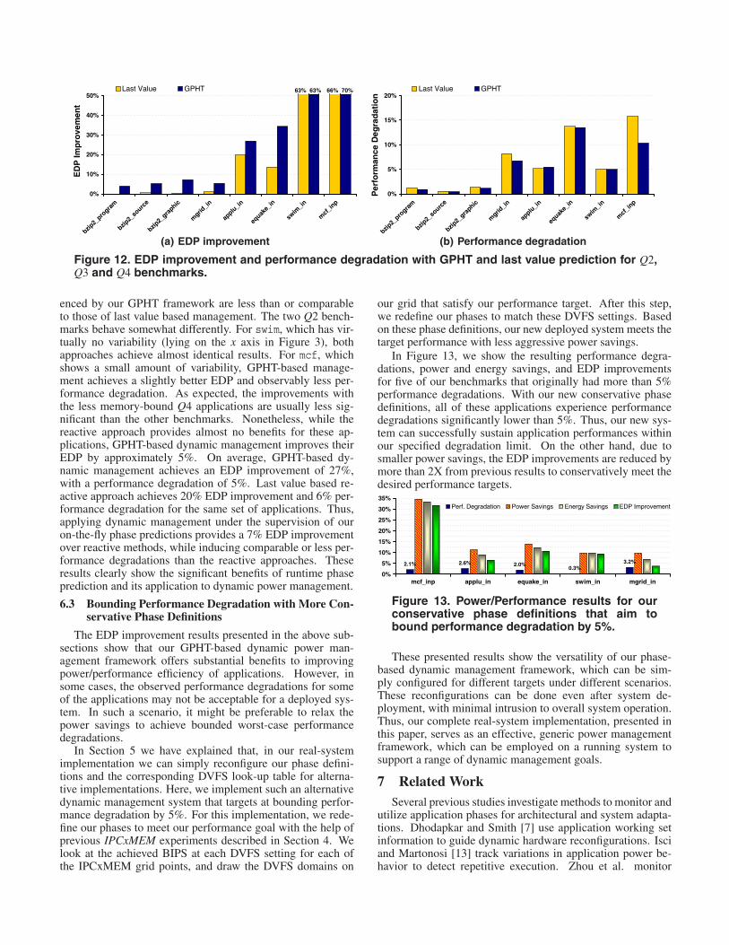
In Figure 12 we show the achieved EDP improvementand performance degradation with both dynamic managementmethods. We show the results for the highly variable Q3 andQ4 benchmarks, as well as the high-power-savings and low-variation Q2 benchmarks. For many of the Q1 applications,the trade-offs with the reactive approach is comparable to ourGPHT-based approach. For these stable applications, respond-ing to previously seen behavior is already the near-optimal ap-proach.

Figure 12 depicts the advantage of employing our dynamicmanagement techniques guided by on-the-fly phase predic-tions. For the variable Q3 and Q4 benchmarks, GPHT-based,proactive management achieves superior EDP improvements,compared to last-value-based, reactive dynamic power man-agement. In general, the performance degradations experi-

0%

10%

20%

30%

40%

50%

bzip2_

progra

m

bzip2_

sourc

e

bzip2_

graphic

mgrid

_in

applu

_in

equak

e_in

swim

_in

mcf

_inp

ED

P Im

pro

vem

ent

Last Value GPHT 63% 63% 66% 70%

(a) EDP improvement

0%

5%

10%

15%

20%

bzip2_

progra

m

bzip2_

sourc

e

bzip2_

graphic

mgrid

_in

applu

_in

equak

e_in

swim

_in

mcf

_inp

Per

form

ance

Deg

rad

atio

n

Last Value GPHT

(b) Performance degradation

Figure 12. EDP improvement and performance degradation with GPHT and last value prediction for Q2,Q3 and Q4 benchmarks.

enced by our GPHT framework are less than or comparableto those of last value based management. The two Q2 bench-marks behave somewhat differently. For swim, which has vir-tually no variability (lying on the x axis in Figure 3), bothapproaches achieve almost identical results. For mcf, whichshows a small amount of variability, GPHT-based manage-ment achieves a slightly better EDP and observably less per-formance degradation. As expected, the improvements withthe less memory-bound Q4 applications are usually less sig-nificant than the other benchmarks. Nonetheless, while thereactive approach provides almost no benefits for these ap-plications, GPHT-based dynamic management improves theirEDP by approximately 5%. On average, GPHT-based dy-namic management achieves an EDP improvement of 27%,with a performance degradation of 5%. Last value based re-active approach achieves 20% EDP improvement and 6% per-formance degradation for the same set of applications. Thus,applying dynamic management under the supervision of ouron-the-fly phase predictions provides a 7% EDP improvementover reactive methods, while inducing comparable or less per-formance degradations than the reactive approaches. Theseresults clearly show the significant benefits of runtime phaseprediction and its application to dynamic power management.

6.3 Bounding Performance Degradation with More Con-servative Phase Definitions

The EDP improvement results presented in the above sub-sections show that our GPHT-based dynamic power man-agement framework offers substantial benefits to improvingpower/performance efficiency of applications. However, insome cases, the observed performance degradations for someof the applications may not be acceptable for a deployed sys-tem. In such a scenario, it might be preferable to relax thepower savings to achieve bounded worst-case performancedegradations.

In Section 5 we have explained that, in our real-systemimplementation we can simply reconfigure our phase defini-tions and the corresponding DVFS look-up table for alterna-tive implementations. Here, we implement such an alternativedynamic management system that targets at bounding perfor-mance degradation by 5%. For this implementation, we rede-fine our phases to meet our performance goal with the help ofprevious IPCxMEM experiments described in Section 4. Welook at the achieved BIPS at each DVFS setting for each ofthe IPCxMEM grid points, and draw the DVFS domains on

our grid that satisfy our performance target. After this step,we redefine our phases to match these DVFS settings. Basedon these phase definitions, our new deployed system meets thetarget performance with less aggressive power savings.

In Figure 13, we show the resulting performance degra-dations, power and energy savings, and EDP improvementsfor five of our benchmarks that originally had more than 5%performance degradations. With our new conservative phasedefinitions, all of these applications experience performancedegradations significantly lower than 5%. Thus, our new sys-tem can successfully sustain application performances withinour specified degradation limit. On the other hand, due tosmaller power savings, the EDP improvements are reduced bymore than 2X from previous results to conservatively meet thedesired performance targets.

2.1% 2.6% 2.0%0.3%

3.2%

0%

5%

10%

15%

20%

25%

30%

35%

mcf_inp applu_in equake_in swim_in mgrid_in

Perf. Degradation Power Savings Energy Savings EDP Improvement

Figure 13. Power/Performance results for ourconservative phase definitions that aim tobound performance degradation by 5%.

These presented results show the versatility of our phase-based dynamic management framework, which can be sim-ply configured for different targets under different scenarios.These reconfigurations can be done even after system de-ployment, with minimal intrusion to overall system operation.Thus, our complete real-system implementation, presented inthis paper, serves as an effective, generic power managementframework, which can be employed on a running system tosupport a range of dynamic management goals.

7 Related WorkSeveral previous studies investigate methods to monitor and

utilize application phases for architectural and system adapta-tions. Dhodapkar and Smith [7] use application working setinformation to guide dynamic hardware reconfigurations. Isciand Martonosi [13] track variations in application power be-havior to detect repetitive execution. Zhou et al. monitor

memory access patterns for energy-efficient memory alloca-tion [30]. Annavaram et al. identify sequential and parallelphases of parallel applications to distribute threads efficientlyon an asymmetric multiprocessor [2]. Weissel and Bellosa alsomonitor memory boundedness of applications to adapt proces-sor execution to different phases on the fly [27]. These worksshow interesting applications for different aspects of applica-tion phase behavior. However, these approaches do not con-sider predicting future phase behavior of applications and per-form adaptive responses reactively, based on most recent be-havior.

Some earlier work also considers prediction of future appli-cation behavior. Duesterwald et al. utilize performance coun-ters to predict certain metric behavior such as IPC and cachemisses based on previous history [8]. They also show that ta-ble based predictors perform significantly better than statisti-cal approaches to predict variable application behavior. Lau etal. consider prediction of phase transitions as well as samplephase durations using different predictors [18]. While theseworks provide significant insights to predictability of applica-tion behavior, they do not evaluate the runtime applicability ofthese predictions to dynamic management.

Sherwood et al. describe a microarchitectural phase pre-dictor based on the traversed basic blocks [24]. They ap-ply this prediction methodology to dynamic cache reconfig-urations and scaling of pipeline resources. This work de-scribes fine-grained, microarchitecture-level phase monitoringand dynamic management, based on architectural simulations,while our work describes a deployed real-system frameworkfor on-the-fly phase prediction of running applications andsystem-level management. Shen et al. detect repetitive phasesat runtime by monitoring reuse distance patterns with applica-tion to cache configurations and memory remapping [21]. Thiswork employs detailed program profiling and instrumentationto detect repetitive phases. In contrast, our work identifies re-current execution and predicts phases seamlessly during nativeapplication execution without prior instrumentations or profil-ing. Wu et al. also describe a real-system implementation ofa runtime DVFS optimizer that monitors application memoryaccesses [28]. This work requires the applications to executefrom within a dynamic instrumentation framework and relieson periodic dynamic profiling of code regions, inducing addi-tional operation overheads. In comparison, our deployed sys-tem operates autonomously on any running application, with-out necessitating any dynamic instrumentation support or priorprofiling, and with no observable overheads to application ex-ecution.

8 ConclusionThis work presents a fully-automated, real-system frame-

work for on-the-fly phase prediction of running applications.These runtime phase predictions are used to guide dynamicvoltage and frequency scaling (DVFS) as the underlying dy-namic management technique on a deployed system.

We experiment with different prediction methods and pro-pose a Global Phase History Table (GPHT) predictor, lever-aged from a common branch predictor architecture. OurGPHT predictor performs accurate on-the-fly phase predic-tions for running applications with no visible overheads. Forhighly variable applications, our GPHT predictor can reducemispredictions by 6X, compared to statistical prediction ap-

proaches. This phase prediction framework efficiently cooper-ates with DVFS to dynamically adapt processor execution tovarying workload behavior. DVFS, guided by these phase pre-dictions, improves the energy-delay product of variable work-loads by as much as 34%, and on average by 18%. Com-pared to previous reactive approaches, our method improvesthe energy-delay product of applications by as much as 20%and on average by 7%.

Our presented results show the promising benefits of run-time phase prediction and its application to dynamic manage-ment. As power management is an increasingly pressing con-cern, the necessity of such workload-adaptive techniques alsoincreases. Our real-system solution, with its energy-saving po-tential and negligible-overhead operation, can serve as a foun-dation for many dynamic management applications in currentand emerging systems.

Acknowledgments

We would like to thank Qiang Wu for his help during thedevelopment of this work and for several useful discussions.We also thank the anonymous reviewers for their useful sug-gestions. This research was supported by NSF grant CNS-0410937. Martonosi’s work is also supported in part by Intel,IBM, SRC and the GSRC/C2S2 joint microarchitecture thrust.

References[1] D. Albonesi, R. Balasubramonian, S. Dropsho, S. Dwarkadas, E. Fried-

man, M. Huang, V. Kursun, G. Magklis, M. Scott, G. Semeraro, P. Bose,A. Buyuktosunoglu, P. Cook, and S. Schuster. Dynamically Tun-ing Processor Resources with Adaptive Processing. IEEE Computer,36(12):43–51, 2003.

[2] M. Annavaram, E. Grochowski, and J. Shen. Mitigating Amdahl’s LawThrough EPI Throttling. In Proceedings of the 32nd International Sym-posium on Computer Architecture (ISCA-32), 2005.

[3] M. Annavaram, R. Rakvic, M. Polito, J.-Y. Bouguet, R. Hankins, andB. Davies. The Fuzzy Correlation between Code and Performance Pre-dictability. In Proceedings of the 37th International Symp. on Microar-chitecture, 2004.

[4] R. D. Barnes, E. M. Nystrom, M. C. Merten, and W. mei W.Hwu. Vac-uum packing: extracting hardware-detected program phases for post-link optimization. In Proceedings of the 35th International Symp. onMicroarchitecture, Nov. 2002.

[5] F. Bellosa, A. Weissel, M. Waitz, and S. Kellner. Event-Driven En-ergy Accounting for Dynamic Thermal Management. In Proceedingsof the Workshop on Compilers and Operating Systems for Low Power(COLP’03), New Orleans, Sept. 2003.

[6] J. Cook, R. L. Oliver, and E. E. Johnson. Examining performance dif-ferences in workload execution phases. In Proceedings of the IEEE In-ternational Workshop on Workload Characterization (WWC-4), 2001.

[7] A. Dhodapkar and J. Smith. Managing multi-configurable hardware viadynamic working set analysis. In 29th Annual International Symposiumon Computer Architecture, 2002.

[8] E. Duesterwald, C. Cascaval, and S. Dwarkadas. Characterizing andPredicting Program Behavior and its Variability. In IEEE PACT, pages220–231, 2003.

[9] S. Gochman, R. Ronen, I. Anati, A. Berkovits, T. Kurts, A. Naveh,A. Saeed, Z. Sperber, and R. C. Valentine. The Intel Pentium M Pro-cessor: Microarchitecture and Performance. Intel Technology Journal,Q2, 2003, 7(02), 2003.

[10] C. Hu, D. Jimenez, and U. Kremer. Toward an Evaluation Infras-tructure for Power and Energy Optimizations. In Workshop on High-Performance, Power-Aware Computing, 2005.

[11] C. Hughes, J. Srinivasan, and S. Adve. Saving energy with architec-tural and frequency adaptations for multimedia applications. In Proceed-ings of the 34th Annual International Symposium on Microarchitecture(MICRO-34), Dec. 2001.

[12] C. Isci and M. Martonosi. Identifying Program Power Phase Behaviorusing Power Vectors. In Proceedings of the IEEE International Work-shop on Workload Characterization (WWC-6), 2003.

[13] C. Isci and M. Martonosi. Detecting Recurrent Phase Behavior underReal-System Variability. In Proceedings of the IEEE International Sym-posium on Workload Characterization, Oct. 2005.

[14] C. Isci, M. Martonosi, and A. Buyuktosunoglu. Long-term WorkloadPhases: Duration Predictions and Applications to DVFS. IEEE Micro:Special Issue on Energy Efficient Design, 25(5):39–51, Sep/Oct 2005.

[15] A. Iyer and D. Marculescu. Power aware microarchitecture resourcescaling. In Proceedings of Design Automation and Test in Europe,DATE, Mar. 2001.

[16] R. Kotla, A. Devgan, S. Ghiasi, T. Keller, and F. Rawson. Characterizingthe Impact of Different Memory-Intensity Levels. In IEEE 7th AnnualWorkshop on Workload Characterization (WWC-7), Oct. 2004.

[17] R. Kotla, S. Ghiasi, T. Keller, and F. Rawson. Scheduling ProcessorVoltage and Frequency in Server and Cluster Systems. In Proceedingsof the 19th IEEE International Parallel and Distributed Processing Sym-posium (IPDPS’05), 2005.

[18] J. Lau, S. Schoenmackers, and B. Calder. Transition Phase Classificationand Prediction. In 11th International Symposium on High PerformanceComputer Architecture, 2005.

[19] C. Luk, R. Cohn, R. Muth, H. Patil, A. Klauser, G. Lowney, S. Wallace,V. Reddi, and K. Hazelwood. Pin: Building Customized Program Anal-ysis Tools with Dynamic Instrumentation. In Programming LanguageDesign and Implementation (PLDI), June 2005.

[20] H. Patil, R. Cohn, M. Charney, R. Kapoor, A. Sun, and A. Karunanidhi.Pinpointing Representative Portions of Large Intel Itanium Programswith Dynamic Instrumentation. In Proceedings of the 37th InternationalSymp. on Microarchitecture, 2004.

[21] X. Shen, Y. Zhong, and C. Ding. Locality Phase Prediction. In EleventhInternational Conference on Architectural Support for ProgrammingLanguages and Operating Systems (ASPLOS XI), Oct. 2004.

[22] T. Sherwood, E. Perelman, and B. Calder. Basic block distributionanalysis to find periodic behavior and simulation points in applications.In International Conference on Parallel Architectures and CompilationTechniques, Sept. 2001.

[23] T. Sherwood, E. Perelman, G. Hamerly, and B. Calder. AutomaticallyCharacterizing Large Scale Program Behavior. In Tenth InternationalConference on Architectural Support for Programming Languages andOperating Systems, Oct 2002.

[24] T. Sherwood, S. Sair, and B. Calder. Phase tracking and prediction. InProceedings of the 28th International Symposium on Computer Archi-tecture (ISCA-30), June 2003.

[25] K. Skadron, M. R. Stan, W. Huang, S. Velusamy, K. Sankaranarayanan,and D. Tarjan. Temperature-aware microarchitecture. In Proceedingsof the 30th International Symposium on Computer Architecture, June2003.

[26] R. Todi. Speclite: using representative samples to reduce spec cpu2000workload. In Proceedings of the IEEE International Workshop on Work-load Characterization (WWC-4), 2001.

[27] A. Weissel and F. Bellosa. Process cruise control: Event-driven clockscaling for dynamic power management. In Proceedings of the Interna-tional Conference on Compilers, Architecture and Synthesis for Embed-ded Systems (CASES 2002), Grenoble, France,, Aug. 2002.

[28] Q. Wu, V. Reddi, Y. Wu, J. Lee, D. Connors, D. Brooks, M. Martonosi,and D. W. Clark. A Dynamic Compilation Framework for ControllingMicroprocessor Energy and Performance. In Proceedings of the 38thInternational Symp. on Microarchitecture, 2005.

[29] T. Y. Yeh and Y. N. Patt. Alternative implementations of two-leveladaptive branch prediction. In 19th Annual International Symposiumon Computer Architecture, May 1992.

[30] P. Zhou, V. Pandey, J. Sundaresan, A. Raghuraman, Y. Zhou, and S. Ku-mar. Dynamic Tracking of Page Miss Ratio Curve for Memory Man-agement. In Proceedings of the 11th International Conference on Archi-tectural Support for Programming Languages and Operating Systems(ASPLOS-XI), 2004.