A Parametric Model for Predicting Submarine Dynamic Stability in Early Stage Design

Lisa Minnick

A thesis submitted to the Faculty of

Virginia Polytechnic Institute and State University

in partial fulfillment of the requirements for the degree of

MASTER OF SCIENCE in

Ocean Engineering

Dr. Alan J. Brown, Chairman Dr. Craig Woolsey Dr. Leigh McCue

April 21, 2006 Blacksburg, Virginia

Keywords: submarine, dynamic stability, design

Copyright 2006, Lisa Minnick

A Parametric Model for Predicting Submarine Dynamic Stability in Early Stage Design

Lisa Minnick

ABSTRACT

The goal of this thesis is to develop a dynamic stability and control module that can

be used in the concept exploration phase of design. The purpose of the module is to

determine the hydrodynamic coefficients/derivatives and stability characteristics of a

given design. Two tools, GEORGE and CEBAXI and LA_57, were used to model a

submarine, calculate its hydrodynamic coefficients, and determine its stability in the

horizontal and vertical plane. GEORGE was developed and used heavily at Naval Coastal

Systems Laboratory (NSWCPC) in Panama City, FL and the CEBAXI and LA_57

program was developed partially at University of California State at Long Beach and at

the Carderock Division of the Naval Surface Warfare Center (NSWCCD) and is in use at

NSWCCD in Bethesda, MD. Both programs require the hull offsets and geometry of the

control surfaces as input. The hull offsets were determined by assuming an idealistic

teardrop shape and a method for sizing control surfaces was developed by using previous

designs to determine sizing trends. ModelCenter software was used to integrate the

methods to determine the offsets and control surface geometry with the stability

programs. A design of experiments was performed to determine the influence of various

input variables on the stability indices and response surface models were created. The

response surfaces were implemented into a Total Ship Systems Engineering optimization

process used in the senior ship design course at Virginia Tech.

ii

Acknowledgements

I would like to express my sincere thanks and appreciation to the following:

Dr. Alan Brown, my chairman, for taking me on as one of his graduate students, for his support and feedback, and being a constant mentor throughout my undergraduate and graduate career.

Dr. Craig Woolsey, my committee member, for his support and willingness to take time to answer any questions I had, especially those relating to stability of underwater vehicles, and taking time to further explain concepts that I needed clarity on. Dr. Leigh McCue, my committee member, for her support, helpful suggestions, and feedback throughout this whole process. Jan Crane, my contact at NSWCPC, who was so gracious to answer all of my questions relating to GEORGE and helping me to troubleshoot the discontinuity in the GEORGE data. Kurt Junghans, Dr. Joan Lewis, and Bowen Jeffries, of the Maneuvering and Controls Division of the Hydromechanics Department at NSWCCD for their hospitality and willingness to help me while I was on-site at NSWCCD using their in-house submarine stability program to collect data. Dr. Thomas Fu of the Maneuvering and Controls Division of the Hydromechanics Department at NSWCCD for putting me in contact with Kurt Junghanas, Dr. Lewis, and Bowen. Jeffries and being willing to help me with whatever I needed. Patrick Ryan and David Cash, my contacts at Northrop Grumman Newport News Shipyard, for their eagerness to help me, answer any general submarine questions I had, and provide with any other contacts that may be beneficial to me. All of my friends who have been extremely supportive, especially Tyson Scofield and Brook Sherman, my officemates; Jesse Panneton and Ingrid Shwaiko for their support and hospitability while I was staying in Washington DC and working at NSWCCD and Brian Cavanaugh for his support and assistance while at NSWCCD; Chris Bassler, truly one of my best friends, for his endless support and encouragement and Maria Dunn, James Dreher, Luisa Coppola, Brian Wolyniak, Roger Zalneraitis, Michael Schwandt, Brian Tesson, Jen Suehs, Aimee Schottler, Derek Dupuis, Christy Marr, Dara Ramey, Emily Rhode, and Sam Wright for all their support. Finally, my family, for their continuous support and love throughout this process and in everything that I embark on.

iii

TABLE OF CONTENTS

TABLE OF CONTENTS........................................................................................................................... IV

TABLE OF FIGURES ............................................................................................................................... VI

APPENDIX A ........................................................................................................................................... VII

APPENDIX B............................................................................................................................................ VII

CHAPTER 1 INTRODUCTION ............................................................................................................ 1 1.1 MOTIVATION ................................................................................................................................... 1 1.2 MULTI-OBJECTIVE AND MULTI-DISCIPLINARY OPTIMIZATION OF SUBMARINES............................. 3

1.2.1 Overall Measure of Effectiveness (OMOE) ............................................................................ 4 1.2.2 Overall Measure of Risk (OMOR) .......................................................................................... 6 1.2.3 Cost......................................................................................................................................... 8 1.2.4 Multi-Objective Genetic Optimization (MOGO) and Results ................................................. 9

1.3 SUBMARINE DYNAMIC STABILITY................................................................................................. 11 1.4 THESIS OBJECTIVES....................................................................................................................... 13 1.5 THESIS OUTLINE............................................................................................................................ 14

CHAPTER 2 SUBMARINE DYNAMIC STABILITY AND CONTROL SURFACES.................. 15 2.1 DYNAMIC STABILITY..................................................................................................................... 15

2.1.1 Equations of Motion and Hydrodynamic Coefficients .......................................................... 15 2.1.2 Stability in the Horizontal Plane [13] .................................................................................. 16 2.1.3 Stability in the Vertical Plane............................................................................................... 20 2.1.4 Summary ............................................................................................................................... 24

2.2 CONTROL SURFACES ..................................................................................................................... 25 2.2.1 Forward Planes .................................................................................................................... 25 2.2.2 Aft Planes.............................................................................................................................. 26 2.2.3 Sail/Fairwater....................................................................................................................... 27

CHAPTER 3 TOOLS USED FOR DETERMINING SUBMARINE DYNAMIC STABILITY..... 29 3.1 GEORGE [10] .............................................................................................................................. 29

3.1.1 Overview............................................................................................................................... 29 3.1.2 Input File .............................................................................................................................. 30 3.1.3 Program Structure................................................................................................................ 31 3.1.4 Output File............................................................................................................................ 32

3.2 CEBAXI AND LA_57 ................................................................................................................... 32 3.2.1 CEBAXI ................................................................................................................................ 33 3.2.2 LA_57 ................................................................................................................................... 33

3.3 CONTROL SURFACES DATABASE................................................................................................... 33 3.3.1 Forward Planes .................................................................................................................... 36

3.3.1.1 GEORGE ......................................................................................................................................... 36 3.3.1.2 CEBAXI and LA_57........................................................................................................................ 38

3.3.2 Fairwater Geometry ............................................................................................................. 38 3.3.2.1 GEORGE ......................................................................................................................................... 38 3.3.2.2 CEBAXI and LA_57........................................................................................................................ 40

3.3.3 Horizontal Stern Planes........................................................................................................ 40 3.3.3.1 GEORGE ......................................................................................................................................... 40 3.3.3.2 CEBAXI and LA_57........................................................................................................................ 42

3.3.4 Vertical Stern Planes ............................................................................................................ 42 3.3.4.1 GEORGE ......................................................................................................................................... 43 3.3.4.2 CEBAXI and LA_57........................................................................................................................ 44

iv

3.3.5 General Procedure ............................................................................................................... 45 3.4 HULL OFFSETS .............................................................................................................................. 52

CHAPTER 4 RESPONSE SURFACE MODEL (RSM) TOOLS ...................................................... 54 4.1 TOOLS FOR ANALYSIS................................................................................................................... 54

4.1.1 ModelCenter ......................................................................................................................... 54 4.1.2 Analysis Server ..................................................................................................................... 55 4.1.3 Design of Experiments Toolkit.............................................................................................. 55 4.1.4 Response Surface Model (RSM) Toolkit ............................................................................... 57 4.1.5 Darwin Optimizer ................................................................................................................. 58

4.2 IMPLEMENTATION OF DYNAMIC STABILITY MODULES IN MODELCENTER.................................... 58 4.2.1 Creating a File Wrapper ...................................................................................................... 59 4.2.2 Link Editor............................................................................................................................ 61 4.2.3 Dynamic Stability Models..................................................................................................... 62

4.2.3.1 GEORGE Model .............................................................................................................................. 62 4.2.3.2 CEBAXI and LA_57 Model............................................................................................................. 63

CHAPTER 5 DESIGN OF EXPERIMENTS RESULTS AND RESPONSE SURFACE MODELS 65

5.1 GEORGE DYNAMIC STABILITY MODEL....................................................................................... 65 5.1.1 Configuration 1: Cruciform Stern ........................................................................................ 65 5.1.2 Configuration 2: X-stern....................................................................................................... 69 5.1.3 Summary and Discussion of Results ..................................................................................... 73

5.2 CEBAXI AND LA_57 DYNAMIC STABILITY MODEL .................................................................... 77 5.2.1 Configuration 1: Sail planes with an X-stern ....................................................................... 78 5.2.2 Configuration 2: X-stern with bow planes............................................................................ 82 5.2.3 Configuration 3: Cruciform Stern with Sail Planes.............................................................. 85 5.2.4 Configuration 4: Cruciform Stern with Bow Planes............................................................. 89 5.2.5 Summary ............................................................................................................................... 93

5.3 GEORGE AND CEBAXI AND LA_57 COMPARISON..................................................................... 94 CHAPTER 6 CONVENTIONAL GUIDED MISSILE SUBMARINE (SSG(X)) DESIGN CASE STUDY 95

6.1 SSG(X) MISSION DEFINITION AND OMOE DEVELOPMENT .......................................................... 95 6.2 SUBMARINE SYNTHESIS MODEL [1] ............................................................................................ 102 6.3 IMPLEMENTATION AND INTEGRATION OF DYNAMIC STABILITY MODELS IN THE SUBMARINE SYNTHESIS MODEL IN MODELCENTER.................................................................................................... 107 6.4 OPTIMIZATION............................................................................................................................. 109 6.5 OPTIMIZATION RESULTS.............................................................................................................. 110

6.5.1 General Results................................................................................................................... 110 6.5.2 Feasibility Results............................................................................................................... 112

CHAPTER 7 CONCLUSIONS........................................................................................................... 115 7.1 DYNAMIC STABILITY MODEL AND CASE STUDY OPTIMIZATION CONCLUSIONS ......................... 115 7.2 SUGGESTIONS FOR FUTURE WORK .............................................................................................. 116

REFERENCES ......................................................................................................................................... 118

APPENDICES .......................................................................................................................................... 120 APPENDIX A - CONTROL SURFACE DATABASE DESIGNS (WWW.COMBATINDEX.COM)............................ 120 APPENDIX B – CONTROL SURFACE DATABASE PLOTS ............................................................................ 125

Control Surface Parameters vs. Length to Diameter Ratio ................................................................ 125 Aspect Ratio vs. Length to Diameter Ratio......................................................................................... 128 Non-Dimensional Delta Chord vs. Length to Diameter Ratio............................................................ 131

VITAE ....................................................................................................................................................... 134

v

TABLE OF FIGURES Figure 1. Design Process [1]........................................................................................................................... 2 Figure 2. Concept Exploration [1]. ................................................................................................................. 2 Figure 3. Submarine Synthesis Model in ModelCenter [1]. ........................................................................... 4 Figure 4. OMOE and OMOR Development Process [1]. ............................................................................... 5 Figure 5. OMOE Hierarchy [1]. ..................................................................................................................... 6 Figure 6. Cost Flowchart. ............................................................................................................................... 9 Figure 7. Multi-Objective Genetic Optimization [1]. ................................................................................... 10 Figure 8. Example of Non-Dominated Frontier [1]. ..................................................................................... 11 Figure 9. Various kinds of motion stability in the vertical plane [2]. ........................................................... 13 Figure 10. Coordinate Reference Frame Definition [12].............................................................................. 16 Figure 11. Stern configurations. ................................................................................................................... 27 Figure 12. Body station definition [10]. ....................................................................................................... 30 Figure 13. GEORGE Flowchart. .................................................................................................................. 32 Figure 14. Top View of Los Angeles class submarine [15]. ........................................................................ 35 Figure 15. Side view of Los Angeles class submarine [15].......................................................................... 35 Figure 16. Forward plane attached to fairwater geometry, top view [10]..................................................... 37 Figure 17. Forward plane attached to fairwater geometry, end view [10]. ................................................... 38 Figure 18. Fairwater geometry, side view (bow is to the left) [10]. ............................................................. 39 Figure 19. Fairwater geometry with forward planes attached, side view (bow is to the left) [10]. .............. 40 Figure 20. Horizontal stern plane geometry, top view [10]. ......................................................................... 42 Figure 21. Horizontal stern plane geometry, side and end views [10].......................................................... 42 Figure 22. Vertical stern plane geometry, side view [10]............................................................................. 44 Figure 23. Generalized trapezoidal shape for control surfaces..................................................................... 47 Figure 24. Teardrop and modified teardrop hullform [4]. ............................................................................ 53 Figure 25. Example of ModelCenter environment. ...................................................................................... 55 Figure 26. DOE Tool. ................................................................................................................................... 57 Figure 27. Example of file wrapper.............................................................................................................. 60 Figure 28. Example of Link Editor user interface. ....................................................................................... 61 Figure 29. GEORGE Dynamic Stability Model. .......................................................................................... 62 Figure 30. NSWCCD Dynamic Stability Model. ......................................................................................... 64 Figure 31. GH main effects plot for GEORGE model with cruciform stern. ................................................ 66 Figure 32. GV main effects plot for GEORGE model with cruciform stern. ................................................ 66 Figure 33. Stability indices vs.L/D for GEORGE model with cruciform stern............................................ 67 Figure 34. GH variable influence for GEORGE model with a cruciform stern............................................. 68 Figure 35. GV variable influence for GEORGE model with a cruciform stern............................................. 68 Figure 36. Gh main effects for GEORGE model with an x-stern................................................................. 70 Figure 37. Gv main effects for GEORGE model with an x-stern................................................................. 70 Figure 38. Stability indices vs. L/D for GEORGE model with an x-stern.................................................... 71 Figure 39. Gh variable influence for GEORGE model with an x-stern........................................................ 72 Figure 40. Gv variable influence for GEORGE model with an x-stern........................................................ 72 Figure 41. Horizontal plane stability derivatives vs. L/D............................................................................. 74 Figure 42. Values of denominator and numerator as a function of L/D. ...................................................... 74 Figure 43. Vertical plane stability derivatives vs L/D. ................................................................................. 75 Figure 44. Denominator and numerator of vertical stability index vs L/D................................................... 76 Figure 45. Stability indices vs. L/D for bare hull. ........................................................................................ 77 Figure 46. Stability indices vs L/D for bare hull data using CEBAXI and LA_57. ..................................... 77 Figure 47. Gh main effects for CEBAXI and LA_57 configuration 1. ........................................................ 79 Figure 48. Gv main effects for CEBAXI and LA_57 configuration 1. ........................................................ 79 Figure 49. Stability indices vs L/D for configuration 1. ............................................................................... 80 Figure 50. Gh variable influence for configuration 1. .................................................................................. 81 Figure 51. Gv variable influence for configuration 1. .................................................................................. 81 Figure 52. Gh main effects for configuration 2. ........................................................................................... 82 Figure 53. Gv main effects for configuration 2. ........................................................................................... 83

vi

Figure 54. Stability indices vs L/D for configuration 2. ............................................................................... 83 Figure 55. Gh variable influence for configuration 2. .................................................................................. 84 Figure 56. Gv variable influence for configuration 2. .................................................................................. 84 Figure 57. Gh main effects for configuration 3. ........................................................................................... 85 Figure 58. Gv main effects for configuration 3. ........................................................................................... 86 Figure 59. Stability indices vs. L/D for configuration 3. .............................................................................. 87 Figure 60. Gh variable influence for configuration 3. .................................................................................. 88 Figure 61. Gv variable influence for configuration 3. .................................................................................. 88 Figure 62. Gh main effects for configuration 4. ........................................................................................... 89 Figure 63. Gv main effects for configuration 4. ........................................................................................... 90 Figure 64. Stability indices vs L/D for configuration 4. ............................................................................... 91 Figure 65. Gh variable influence for configuration 4. .................................................................................. 92 Figure 66. Gv variable influence for configuration 4. .................................................................................. 92 Figure 67 . OMOE Hierarchy ..................................................................................................................... 102 Figure 68: Submarine balance work flow diagram [1]. .............................................................................. 105 Figure 69. VOP for Gh. .............................................................................................................................. 108 Figure 70. VOP for Gv. .............................................................................................................................. 108 Figure 71. 3-D Non-Dominated Frontier.................................................................................................... 111 Figure 72. 3-D NDF showing risk bands.................................................................................................... 111 Figure 73. 2-D Non-Dominated Frontier.................................................................................................... 112 Figure 74. Optimization Results: Stability Indices vs. L/D........................................................................ 113 Figure 75. Optimization Results: Forward plane configuration. ................................................................ 113 Figure 76. Optimization Results: Stern plane configuration. ..................................................................... 114 Figure 77. SSG(X) Rhino drawing [1]. ...................................................................................................... 116

APPENDIX A Figure A1. Top view of Benjamin Franklin class submarine. .................................................................... 120 Figure A2. Side view of Benjamin Franklin class submarine. ................................................................... 120 Figure A3. Top view of George Washington class submarine. .................................................................. 120 Figure A4. Side view of George Washington class submarine................................................................... 120 Figure A5. Top view of Ohio class submarine. .......................................................................................... 121 Figure A6. Side view of Ohio class submarine. ......................................................................................... 121 Figure A7. Top View of Lafayette class submarine. .................................................................................. 121 Figure A8. Side view of Lafayette class submarine. .................................................................................. 121 Figure A9. Top view of Permit class submarine. ....................................................................................... 121 Figure A10. Side view of Permit class submarine...................................................................................... 122 Figure A11. Top view of Seawolf class submarine. ................................................................................... 122 Figure A12. Side view of Seawolf class submarine. .................................................................................. 122 Figure A13. Top view of Skipjack class submarine. .................................................................................. 122 Figure A14. Side view of Skipjackt class submarine. ................................................................................ 123 Figure A15. Top view of Sturgeon class submarine................................................................................... 123 Figure A16. Side view of Sturgeon class submarine. ................................................................................. 123 Figure A17. Top view of Virginia class submarine.................................................................................... 123 Figure A18. Side view of Virginia class submarine. .................................................................................. 124

APPENDIX B Figure B1. Control surface parameter vs. L/D for forward planes. ............................................................ 125 Figure B2. Control surface parameter vs. L/D for Horizontal Stern Planes. .............................................. 125 Figure B3. Control surface parameter vs. L/D for upper vertical stern planes. .......................................... 126 Figure B4. Control surface parameter vs. L/D for the lower vertical stern plane....................................... 127 Figure B5. Control surface parameter vs. L/D ratio for the sail. ................................................................ 127 Figure B6. AR vs L/D for the forward planes. ........................................................................................... 128 Figure B7. AR vs L/D for horizontal stern planes...................................................................................... 129

vii

Figure B8. AR vs. L/D for upper vertical stern plane................................................................................. 129 Figure B9. AR vs. L/D for lower vertical stern plane................................................................................. 130 Figure B10. AR vs. L/D for the sail. .......................................................................................................... 130 Figure B11. Non-dimensional delta chord vs. L/D for forward planes. ..................................................... 131 Figure B12. Non-dimensional delta chord vs. L/D for horizontal stern planes .......................................... 131 Figure B13. Non-dimensional delta chord vs. L/D for upper vertical stern plane...................................... 132 Figure B14. Non-dimensional delta chord vs. L/D for lower vertical stern plane...................................... 132 Figure B15. Non-dimensional delta chord vs. L/D for the sail................................................................... 133

viii

TABLE OF TABLES Table 1. Event Probability Estimate [1]. ........................................................................................................ 7 Table 2. Event Consequence Estimate [1]. ..................................................................................................... 8 Table 3. Cost Module Input Variables [1]. ..................................................................................................... 9 Table 4. Summary of designs measured for control surface database. ......................................................... 34 Table 5. Summary of forward plane geometry needed for GEORGE. ......................................................... 36 Table 6. Summary of fairwater geometry needed for GEORGE.................................................................. 39 Table 7. Summary of horizontal stern plane geometry needed for GEORGE.............................................. 40 Table 8. Summary of geometry for upper and lower vertical stern planes for GEORGE. ........................... 43 Table 9. Basic definitions. ............................................................................................................................ 45 Table 10. Calculated non-dimensional mean aerodynamic chord vs. measured .......................................... 47 Table 11. Non-Dimensional x-distance measured from vessel nose. ........................................................... 49 Table 12. DOE variables and high and low boundaries for GEORGE stability model. ............................... 65 Table 13. Summary of RSM statistical data for GEORGE model................................................................ 69 Table 14. Statistical summary for RSM results for GEORGE model with an x-stern.................................. 73 Table 15. Design variables and high and low boundaries for CEBAXI and LA_57 stability model. .......... 78 Table 16. Statistical summary of RSM results for configuration 1. ............................................................. 82 Table 17. Statistical summary of RSM results for configuration 2. ............................................................. 85 Table 18. Statistical summary of RSM results for configuration 3. ............................................................. 89 Table 19. Statistical summary of RSM results for configuration 4. ............................................................. 93 Table 20. ISR Mission Scenario [1]. ............................................................................................................ 95 Table 21. Missile Mission Scenario [1]........................................................................................................ 96 Table 22 - ROC/MOP/DV Summary [1]...................................................................................................... 96 Table 23. MOP Table [1]............................................................................................................................ 101 Table 24. SSG(X) Design Variables (DVs)................................................................................................ 109

ix

CHAPTER 1 INTRODUCTION

1.1 Motivation

The ship design process shown in Figure 1 consists of five main stages: Concept Exploration,

Concept Development, Preliminary Design, Contract Design, and Detail Design. The concept

exploration phase of the design process is detailed in Figure 2 and begins once a mission need

has been determined. It involves translating the need into specific engineering terms and design

variables, determining technology and design alternatives, and identifying the design space to be

used for ship synthesis and optimization. The result is a baseline design that can be analyzed in

greater detail during concept development. This thesis focuses on the concept exploration phase

of the total design process.

Traditional approaches to submarine design have been guided primarily by experience,

design lanes, and rules-of-thumbs. A Total Ship System Engineering (TSSE) approach has been

developed at Virginia Tech to be used in early stage design for surface ships and a similar

approach is being developed for submarines. The TSSE approach views the ship as a

supersystem comprised of various systems, subsystems, and components functioning together to

achieve a common objective [3]. The goal is to optimize the total ship over its lifecycle based on

the objective attributes of cost, risk, and effectiveness. The current submarine synthesis model

developed for this purpose takes into account a number of different design variables such as

hullform, propulsion, and combat systems with measures of performance (MOPs) for speed,

endurance, and diving depth. However, it does not consider dynamic stability and control.

Dynamic stability is a difficult aspect to include in early stage submarine design. It is

dependent on the hydrodynamic coefficients and stability derivatives of the submarine which are

functions of a submarine’s hullform and control surfaces. These coefficients and derivatives are

traditionally determined from analysis and model tests once detailed aspects of the design have

been determined and set. In addition, the specifications of each control surface are generally

considered during later stages of the design process and therefore not typically a part of the

optimization process during concept exploration. The motivation for this thesis is to develop a

dynamic stability module that will evaluate stability by considering hullform and control surface

parameters early in the design process.

1

ConceptExploration

ConceptDevelopment

PreliminaryDesign

ContractDesign

DetailDesign

ExploratoryDesign

Mission orMarketAnalysis

Concept andRequirements

Exploration

TechnologyDevelopment

ConceptDevelopment

and FeasibilityStudiesConcept

BaselineFinalConcept

Figure 1. Design Process [1].

Figure 2. Concept Exploration [1].

2

1.2 Multi-Objective and Multi-Disciplinary Optimization of Submarines

In early stage design, the design space (i.e. the number of possible combinations and values

of the various design variables, either continuous or discrete) is typically very large. Evaluating

the performance of designs for even a small portion of this large design space can become

prohibitive if the analyses are computationally expensive. Because of this, higher-fidelity codes

are typically not used in the early stages of the design process. Major decisions regarding the

basic elements of the design are already made before higher-fidelity codes begin to be used.

At Virginia Tech, during the concept exploration phase, a synthesis model is developed and

an optimization process is used to aid in exploring the design space. The submarine synthesis

model is used to balance and assess designs during optimization. Specific modules in the model

(weights, hullform, space available, propulsion, etc.) are developed using FORTRAN, and are

integrated and executed in ModelCenter (MC). A Multi-Objective Genetic Optimization

(MOGO) is run in MC using a Darwin optimization plug-in. A flowchart for the synthesis model

in MC is shown in Figure 3. Each box represents a design module and the lines connecting each

module show how the inputs and outputs of the modules relate to one another. The process

begins by generating a unique set of inputs that are provided to the individual modules. Within

each module a number of functions are performed and outputs are generated. These outputs are

then supplied to other modules that rely on those outputs as inputs and are also linked to the last

four modules (feasibility, effectiveness, cost, and risk) where effectiveness, cost and risk are the

attributes by which each design is measured. These attribute modules then produce their own

outputs that are input to the optimizer, which works to maximize the effectiveness of the design

while complying with constraints set by the feasibility module and minimizing cost and risk.

Multi-objective optimization of naval ships focuses on three primary objective attributes: life

cycle cost, military effectiveness, and the technology risk associated with the design (cost,

performance risk, and schedule). In order to carry out the optimization, quantitative objective

functions are developed for each specified objective attribute. These functions are developed and

described in more detail in Sections 1.2.1, 1.2.2, and 1.2.3.

3

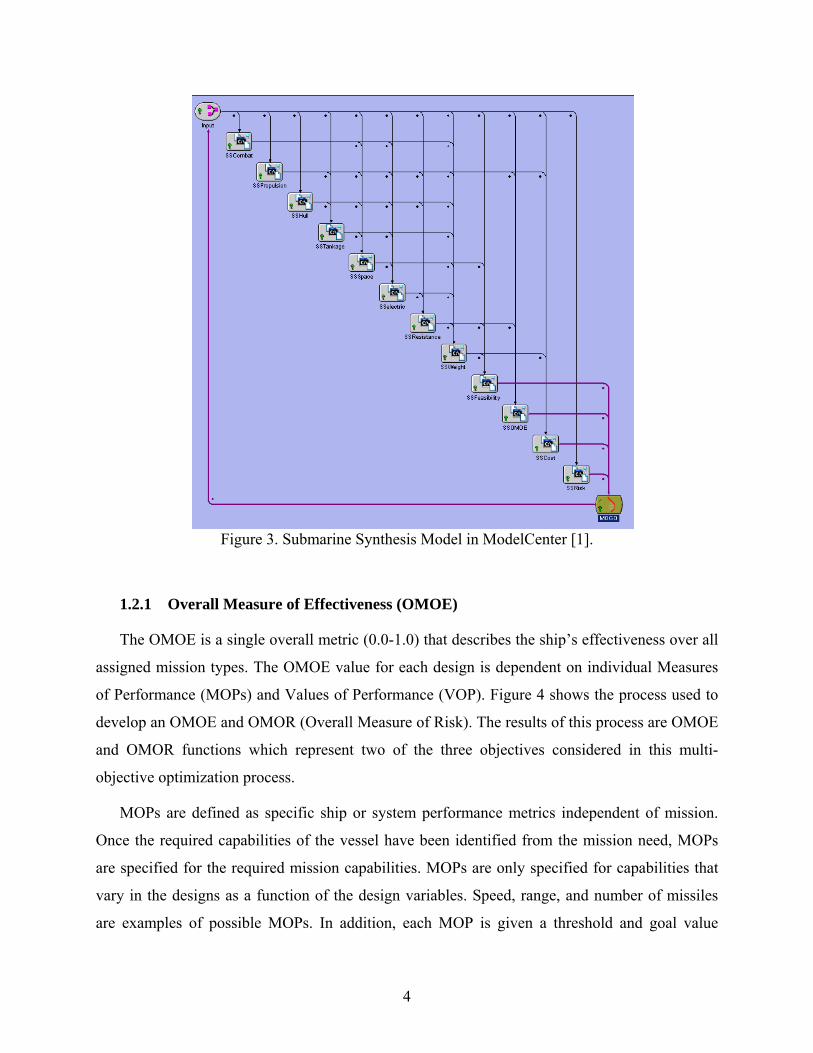
Figure 3. Submarine Synthesis Model in ModelCenter [1].

1.2.1 Overall Measure of Effectiveness (OMOE)

The OMOE is a single overall metric (0.0-1.0) that describes the ship’s effectiveness over all

assigned mission types. The OMOE value for each design is dependent on individual Measures

of Performance (MOPs) and Values of Performance (VOP). Figure 4 shows the process used to

develop an OMOE and OMOR (Overall Measure of Risk). The results of this process are OMOE

and OMOR functions which represent two of the three objectives considered in this multi-

objective optimization process.

MOPs are defined as specific ship or system performance metrics independent of mission.

Once the required capabilities of the vessel have been identified from the mission need, MOPs

are specified for the required mission capabilities. MOPs are only specified for capabilities that

vary in the designs as a function of the design variables. Speed, range, and number of missiles

are examples of possible MOPs. In addition, each MOP is given a threshold and goal value

4

corresponding respectively to the minimum and maximum level of performance. The goal value

is typically determined by a technology limitation or as the point of diminishing marginal value.

MissionDescription

OMOE Hierarchy

ROCs

Requirements and constraints for all

designs

MOPs,Goals &

Thresholds

DPs

VOPFunctions

OMOEFunction

MOPweights

MAVT

AHP

OMOR Hierarchy

Cost Model

Tentative Schedule

AHP

OMOR Weights

OMOR Function

Probabilities and

Consequences

Risk Index

Figure 4. OMOE and OMOR Development Process [1].

An OMOE hierarchy is developed once the required missions for the submarine have been

determined. It groups the MOPs defined to assess the submarine’s ability to meet its mission

requirements into various categories. An example of an OMOE hierarchy is shown in Figure 5.

The hierarchy is developed using an Analytical Hierarchy Process (AHP) which involves pair-

wise comparison questionnaires that solicit expert and customer opinion. From this hierarchy and

process MOP weights are calculated for each MOP and used to develop the individual MOP

value functions.

5

ISR or Missile Launch

War Fighting Mobility

Susceptibility

AAW ASW

ASuW MIW

CCC INT

STK

Sprint Speed

Sprint Endurance

Depth

Environmental

Structure

Acoustic Signature IR Signature

Magnetic Signature

Endurance Snorkel Speed

Endurance AIP

Endurance Snorkel

Ts (Stores)

Sustainability

Dynamic Stability

Figure 5. OMOE Hierarchy [1].

Each MOP has a corresponding VOP. A VOP is a figure of merit index ranging from zero to

one specifying the value of a specific level of performance. A VOP function, typically an S-

curve, is developed for each MOP and used in the ship synthesis model to calculate each VOP.

The VOP value of zero corresponds to the MOP threshold while a value of one corresponds to

the MOP goal. The MOP weights and VOP functions are combined into a single OMOE function

shown in Equation 1:

( )[ ] ( )iii

iii MOPVOPwMOPVOPgOMOE ∑== (1)

1.2.2 Overall Measure of Risk (OMOR)

Three types of technology risk events are considered when calculating the OMOR:

performance, cost, and schedule. Once the ship’s missions, required capabilities, and technology

6

options have been defined these options and associated design variables are assessed for their

contribution to overall risk. In addition, MOP weights, tentative ship and technology

development schedules, and cost predictions are also considered. Risk events are identified with

associated design variables, required capabilities, cost, and schedule. Like OMOE, AHP and a

pair-wise comparison are performed to gather expert opinion and develop OMOR hierarchy

weights. Previously calculated OMOE hierarchy weights associated with risk events are

normalized to a total of 1.0 and reused in the OMOR calculations. After risk events have been

identified a probability of occurrence, Pi, and consequence of occurrence, Ci, are estimated for

each event using the guidelines outlined in Table 1 and Table 2. OMOR is then a function of the

weights and probabilities and listed in Equation 2:

kkk

kschedjjj

jtiii

ii

iperf CPwWCPwWCP

ww

WOMOR ∑∑∑∑++= cos

(2)

Table 1. Event Probability Estimate [1].

Probability What is the Likelihood the Risk Event Will Occur?

0.1 Remote 0.3 Unlikely 0.5 Likely 0.7 Highly likely 0.9 Near Certain

7

Table 2. Event Consequence Estimate [1].

Consequence Level

Given the Risk is Realized, What Is the Magnitude of the Impact?

Performance Schedule Cost

0.1 Minimal or no impact Minimal or no impact Minimal or no impact

0.3 Acceptable with some reduction in margin

Additional resources required; able to meet need dates

<5%

0.5 Acceptable with significant reduction in margin

Minor slip in key milestones; not able to meet need date

5-7%

0.7 Acceptable; no remaining margin

Major slip in key milestone or critical path impacted

7-10%

0.9 Unacceptable Can’t achieve key team

or major program milestone

>10%

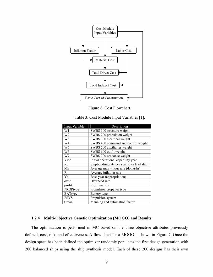
1.2.3 Cost

The components considered in the calculation of the Basic Cost of Construction (BCC) are

shown in Figure 6. BCC is dependent on input variables, listed in Table 3, an inflation factor,

labor costs, material costs, and total direct and indirect costs. The inflation rate is an average

inflation rate based on the number of years between the initial costing and base year. The labor

cost is determined using the ship work breakdown structure (SWBS) weights, complexity

factors, and the man-hour rate. The material cost is a function of SWBS weights, material cost

factors, inflation factor, battery type, propulsion propeller type, and manning and automation

factor. The total direct cost is the sum of total labor cost and total material cost. The total indirect

cost is determined by multiplying the total direct cost by the overhead rate. The BCC is then

determined by summing the total direct and indirect cost and multiplying by one plus the profit

margin.

8

Cost Module Input Variables

Labor CostInflation Factor

Material Cost

Total Direct Cost

Total Indirect Cost

Basic Cost of Construction

Figure 6. Cost Flowchart.

Table 3. Cost Module Input Variables [1].

Input Variable Description W1 SWBS 100 structure weight W2 SWBS 200 propulsion weight W3 SWBS 300 electrical weight W4 SWBS 400 command and control weight W5 SWBS 500 auxiliaries weight W6 SWBS 600 outfit weight W7 SWBS 700 ordnance weight Yioc Initial operational capability year Rp Shipbuilding rate per year after lead ship Mh Average man – hour rate (dollar/hr) R Average inflation rate Yb Base year (appropriation) ovhd Overhead rate profit Profit margin PROPtype Propulsion propeller type BATtype Battery type PSYS Propulsion system Cman Manning and automation factor

1.2.4 Multi-Objective Genetic Optimization (MOGO) and Results

The optimization is performed in MC based on the three objective attributes previously

defined; cost, risk, and effectiveness. A flow chart for a MOGO is shown in Figure 7. Once the

design space has been defined the optimizer randomly populates the first design generation with

200 balanced ships using the ship synthesis model. Each of these 200 designs has their own

9

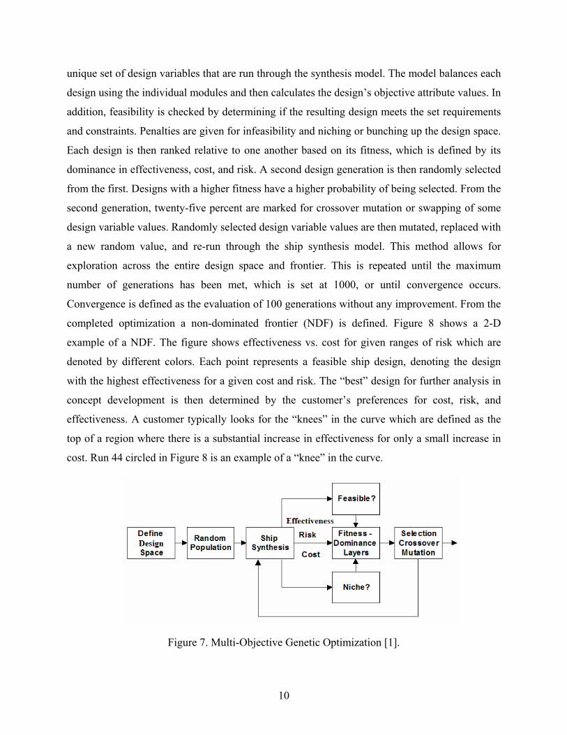
unique set of design variables that are run through the synthesis model. The model balances each

design using the individual modules and then calculates the design’s objective attribute values. In

addition, feasibility is checked by determining if the resulting design meets the set requirements

and constraints. Penalties are given for infeasibility and niching or bunching up the design space.

Each design is then ranked relative to one another based on its fitness, which is defined by its

dominance in effectiveness, cost, and risk. A second design generation is then randomly selected

from the first. Designs with a higher fitness have a higher probability of being selected. From the

second generation, twenty-five percent are marked for crossover mutation or swapping of some

design variable values. Randomly selected design variable values are then mutated, replaced with

a new random value, and re-run through the ship synthesis model. This method allows for

exploration across the entire design space and frontier. This is repeated until the maximum

number of generations has been met, which is set at 1000, or until convergence occurs.

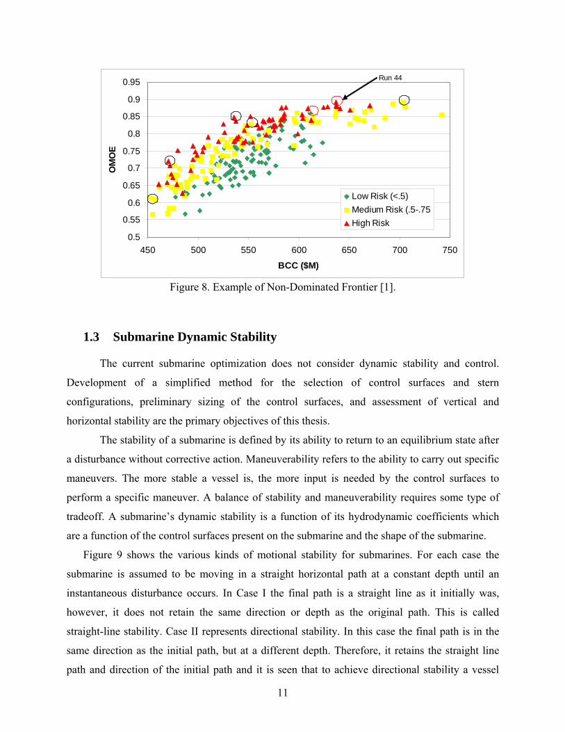
Convergence is defined as the evaluation of 100 generations without any improvement. From the

completed optimization a non-dominated frontier (NDF) is defined. Figure 8 shows a 2-D

example of a NDF. The figure shows effectiveness vs. cost for given ranges of risk which are

denoted by different colors. Each point represents a feasible ship design, denoting the design

with the highest effectiveness for a given cost and risk. The “best” design for further analysis in

concept development is then determined by the customer’s preferences for cost, risk, and

effectiveness. A customer typically looks for the “knees” in the curve which are defined as the

top of a region where there is a substantial increase in effectiveness for only a small increase in

cost. Run 44 circled in Figure 8 is an example of a “knee” in the curve.

Figure 7. Multi-Objective Genetic Optimization [1].

10

0.5

0.55

0.6

0.65

0.7

0.75

0.8

0.85

0.9

0.95

450 500 550 600 650 700 750

BCC ($M)

OM

OE

Low Risk (<.5)Medium Risk (.5-.75High Risk

Run 44

Figure 8. Example of Non-Dominated Frontier [1].

1.3 Submarine Dynamic Stability

The current submarine optimization does not consider dynamic stability and control.

Development of a simplified method for the selection of control surfaces and stern

configurations, preliminary sizing of the control surfaces, and assessment of vertical and

horizontal stability are the primary objectives of this thesis.

The stability of a submarine is defined by its ability to return to an equilibrium state after

a disturbance without corrective action. Maneuverability refers to the ability to carry out specific

maneuvers. The more stable a vessel is, the more input is needed by the control surfaces to

perform a specific maneuver. A balance of stability and maneuverability requires some type of

tradeoff. A submarine’s dynamic stability is a function of its hydrodynamic coefficients which

are a function of the control surfaces present on the submarine and the shape of the submarine.

Figure 9 shows the various kinds of motional stability for submarines. For each case the

submarine is assumed to be moving in a straight horizontal path at a constant depth until an

instantaneous disturbance occurs. In Case I the final path is a straight line as it initially was,

however, it does not retain the same direction or depth as the original path. This is called

straight-line stability. Case II represents directional stability. In this case the final path is in the

same direction as the initial path, but at a different depth. Therefore, it retains the straight line

path and direction of the initial path and it is seen that to achieve directional stability a vessel

11

must also have straight line stability. Case III is similar to Case II in that the final path is the

same that is reached in Case II, however, the vessel does not oscillate after the disturbance as in

Case II. This is because the system in Case II is under-damped, having complex eigenvalues that

cuase the system to oscillate at a damped frequency before returning to equilibrium. Finally,

Case IV represents positional motion stability. In this case the submarine’s final path is in the

same direction and at the same depth as the initial path. Positional motion stability involves a

combination of straight line and directional stability. It is important to note that straight line

stability is determined from a second-order differential equation, directional stability from a

third-order equation, and positional motion stability from a fourth-order differential equation.

The control surfaces of an underwater vehicle are designed to ensure stability in the

horizontal and vertical planes and to provide sufficient control for maneuvering. This thesis only

examines controls-fixed stability where the positions of the control surfaces are fixed and not

varied. In the horizontal plane with the controls-fixed only straight-line stability can be achieved

and as noted above will be determined from a second-order differential equation. Vertical

stability can require both straight-line and directional stability. The scope of this thesis is to

determine if a given submarine design has stability in both the horizontal and vertical planes.

12

Figure 9. Various kinds of motion stability in the vertical plane [2].

1.4 Thesis Objectives The primary objectives of this thesis are to:

• Investigate, document and summarize existing literature in evaluating submarine dynamic

stability, specifically in early stage design.

• Develop a model to perform preliminary sizing of control surfaces for different control

and stern configurations and calculate the hydrodynamic coefficients needed to determine

the dynamic stability of a conventional submarine using two different tools.

• Compare the accuracy and effectiveness of the tools utilized.

• Use sensitivity analysis to refine and screen variable inputs to calculate dynamic stability.

• Develop flexible response surface models (RSMs) for estimating submarine dynamic

stability in the early stages of design.

• Apply these RSMs to a submarine design optimization case study.

• Assess the results.

13

1.5 Thesis Outline

Chapter 1 provides an introduction and motivation for this thesis and provides a background

on the TSSE design process used at Virginia Tech and submarine dynamic stability.

Chapter 2 summarizes the theory used to develop stability indices used in the analysis of

submarine dynamic stability.

Chapter 3 describes the tools used for modeling and analyzing early stage dynamic stability

and summarizes the information needed for each tool to calculate the derived stability indices.

Chapter 4 details the process and tools used to perform the sensitivity analysis and variable

screening and to develop the response surface models.

Chapter 5 analyzes and discusses the results of the sensitivity analysis and the response

surfaces that were created.

Chapter 6 provides a case study for the Conventional Guided Missile (SSG(X)) Submarine.

Chapter 7 presents results and conclusions.

14

CHAPTER 2 SUBMARINE DYNAMIC STABILITY AND CONTROL SURFACES

2.1 Dynamic Stability

2.1.1 Equations of Motion and Hydrodynamic Coefficients

Figure 10 defines the coordinate system used in this analysis. The origin is placed at the

center of gravity (CG) of the submarine. The x-axis is the longitudinal axis and positive towards

the bow. The y-axis is the lateral axis and positive starboard and the z-axis, determined by the

right-hand rule, is positive downward. The three components of the hydrodynamic forces in the

x, y, and z directions are denoted X, Y, and Z respectively while the hydrodynamic torques are

denoted by L (roll), M (pitch), and N (yaw) respectively. The components of the velocity in the

x, y, and z directions are u, v, w respectively and the angular velocities are p, q, and r as shown

in Figure 10.

The hydrodynamic derivatives/coefficients are used to approximate the forces and moments

acting on the vessel. This approach assumes that the motions of the body are small deviations

from straight line motion. Based on this assumption the forces and moments acting on the body

due to a small perturbation can be approximated as directly proportional to the associated small

change in velocity. For example, for a small sway velocity, v, the resulting hydrodynamic force

in the lateral direction acting on the body, Y, can be approximated by the product Yvv, where Yv

represents the sensitivity of the lateral force to changes in sway velocity and is defined as the

partial derivative of the lateral force with respect to the sway velocity evaluated at the nominal

condition, vY∂∂ , and v is the sway velocity encountered by the vessel. The partial derivative is the

hydrodynamic derivative or hydrodynamic coefficient. The hydrodynamic coefficients are useful

in determining a submarine’s dynamic stability.

15

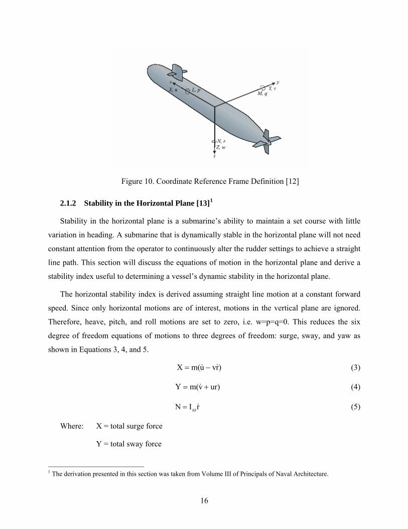
Figure 10. Coordinate Reference Frame Definition [12]

2.1.2 Stability in the Horizontal Plane [13]1

Stability in the horizontal plane is a submarine’s ability to maintain a set course with little

variation in heading. A submarine that is dynamically stable in the horizontal plane will not need

constant attention from the operator to continuously alter the rudder settings to achieve a straight

line path. This section will discuss the equations of motion in the horizontal plane and derive a

stability index useful to determining a vessel’s dynamic stability in the horizontal plane.

The horizontal stability index is derived assuming straight line motion at a constant forward

speed. Since only horizontal motions are of interest, motions in the vertical plane are ignored.

Therefore, heave, pitch, and roll motions are set to zero, i.e. w=p=q=0. This reduces the six

degree of freedom equations of motions to three degrees of freedom: surge, sway, and yaw as

shown in Equations 3, 4, and 5.

)rvum(X && −= (3)

ur)vm(Y += & (4)

rIN zz&= (5)

Where: X = total surge force

Y = total sway force

1 The derivation presented in this section was taken from Volume III of Principals of Naval Architecture.

16

N = total yaw moment

m = mass of submarine

u = surge velocity

u& = surge acceleration

v = sway velocity

v& = sway acceleration

r = yaw rate

r&= yaw acceleration

zzI = moment of inertia about the z-axis

The left hand side of Equations 3, 4, and 5, which represent the total force and moment in the

given degree of freedom, are functions of the surge velocity and acceleration, sway velocity and

acceleration, and yaw rate and acceleration:

)rr,,vv,,u(u,FX x &&&= (6)

)rr,,vv,,u(u,FY Y &&&= (7)

)rr,,vv,,u(u,FN N &&&= (8)

A Taylor series expansion is performed to reduce Equations 6, 7, and 8 into useful mathematical

form. An example of the Taylor series expansion for the total sway force is shown below:

rY)rr(

rY)r(r

vY)vv(

vY)v(v

uY)uu(

uY)u(uYY ooooooo &

&&&

&&&

&&∂∂

−+∂∂

−+∂∂

−+∂∂

−+∂∂

−+∂∂

−+= (9)

The zero subscript denotes values at the nominal condition (straight-line motion with constant

forward speed) and each partial derivative is evaluated at this condition. Since the reference

condition is constant forward speed, the accelerations are zero, therefore . Due to

port/starboard symmetry v

0rvu === &&&

o=0, 0uY

uY

=∂∂

=∂∂

&, and Yo=0. Based on these assumptions Equation 9

becomes:

rYr

rYr

vYv

vYvY

&&

&&

∂∂

+∂∂

+∂∂

+∂∂

= (10)

17

The same process is applied to the total surge force and yaw moment. For yaw, port/starboard

symmetry dictates that 0uN

uN

=∂∂

=∂∂

&, therefore the total yaw moment can be represented as:

rNr

rNr

vNv

vNvN

&&

&&

∂∂

+∂∂

+∂∂

+∂∂

= (11)

Similarly for surge, 0rX

rX

vX

vX

=∂∂

=∂∂

=∂∂

=∂∂

&& because of port/starboard symmetry and the total

surge force becomes:

uuXu

uXX &

&∂∂

+∂∂

= (12)

Equation 12 shows that surge has been decoupled from sway and yaw and can be neglected for

the remainder of the derivation. Substituting Equations 10 and 11 into Equations 3 and 5,

rearranging, and applying the derivative notation yields:

0rYmU)r(Yv)Y(mvY rrvv =−−−−+− && && (13)

0r)N(IrNvNvN rzzrvv =−+−−− && && (14)

These equations are the linearized equations of motion for the sway velocity and yaw rate. It is

important to note that there are no added forces or moments due to the control surfaces since

controls-fixed stability (zero-angle of attack) is assumed. Equations 13 can be non-

dimensionalized by dividing through by 2VρL 22

and Equation 14 can be non-dimensionalized by

2VρL 23

. The resulting equations are:

0'rY')r'm'(Y''v)Y'(m'v'Y' rrvv =−−−−+− && && (15)

0'r)N'(I'r'N''vN'v'N' rzzrvv =−+−−− && && (16)

The superscript prime denotes a non-dimensionalized term. is defined as the virtual mass

coefficient and acts like an added mass. It is the hydrodynamic force that is a result of the

acceleration of the body through the fluid. Similarly, is the virtual moment of inertia

coefficient.

vY' &

rN'&

18

Equations 15 and 16 are coupled in sway and yaw, solving this set of linear equations

results in a second order linear homogeneous equation. The solution for and can be

determined assuming the standard solution for a second order differential equation:

v' r'

σtvev'= (17)

σtrer'= (18)

The constants v and r can be determined from initial conditions and e =2.718. Equations 17 and

18 show that for stability the real part of the exponent σ needs to be negative. If the real part of

sigma is positive then and will increase with increasing time and the initial equilibrium

state will not be reached. If the real part of σ is negative then and will decrease with

increasing time and the system will return to its initial state.

v' r'

v' r'

A relationship between σ and the stability derivatives can be derived by substituting the

solutions obtained using Equations 17 and 18 into Equations 15 and 16 and looking at the

resulting characteristic polynomial:

0CBσAσ2 =++ (19)

Where the coefficients are defined as:

vrrv

rvvrzz

vrzz

)N'm'(Y'N'Y'C)N'Y'(m')Y'N'(I'B

)Y')(m'N'(I'A

−−=−−−−=

−−=

&&

&&

(20)

And σ is determined by the quadratic formula:

( )2A

4ACBBσ2 −±−

= (21)

Routh stability criteria [9] requires that the coefficients A, B, and C have the same sign.

Experimental data show that A and B are always positive, therefore C must be positive:

0)N'm'(Y'N'Y' vrrv >−− (22)

Or

vrrv )N'm'(Y'N'Y' −> (23)

Dividing through by and ( ) yields, vY' m'Y'r−

19

0Y'N'

)m'(Y'N'

v

v

r

r >−−

(24)

The first term in Equation 24 is the ratio of the moment due to rotational motion to the force due

to rotational motion which can also be seen as a measure of the point of action of the rotational

force. The second term is the ratio of the moment due to the sway motion to the force due to

sway or the point at which the force due to sway acts. Therefore, Equation 24 requires for

stability that the force due to yaw rotational motion act at a point further forward than the force

due to sway.

Equation 24 can be modified to represent a stability index,

rv

rvH N'Y'

)m'(Y'N'1G −−= (25)

As long as GH is positive the submarine is stable. As the index approaches zero the damping ratio

decreases, decreasing the stability of the submarine in the horizontal plane. As the index

approaches one the submarine becomes more stable, increasing stability while decreasing the

submarine’s maneuverability characteristics. Based on previous designs and rules of thumb GH

should fall in the range of 0.15 to 0.30 to ensure a good tradeoff between stability and

maneuverability.

2.1.3 Stability in the Vertical Plane

Stability in the vertical plane relates to a submarine’s ability to maintain a steady depth

without continuous activity of the hydroplanes. This characteristic is particularly important at

deep submergence when little can be done to vary the external hydrodynamic forces acting on

the submarine. Therefore, a submarine’s innate dynamic stability plays an important role. This

section will discuss the vertical equations of motion and derive a stability index useful in

assessing the dynamic stability of a submarine in the vertical plane.

The vertical stability index is derived assuming straight line motion at a constant forward

speed. Since only vertical motions are of interest, motions in the horizontal plane are ignored.

Therefore, surge, sway and yaw motions are set to zero, i.e. x=y=r=0. This reduces the six degree

of freedom equations of motions to three degrees of freedom: heave, roll, and pitch as shown in

Equations 26, 27, and 28.

qU)wm(Z −= & (26)

20

pIL xx &= (27)

qIM yy &= (28)

Where: Z = total heave force

L = total roll moment

M = total pitch moment

m = mass of submarine

U = constant forward velocity

w& = heave acceleration

q = pitch velocity

q& = pitch acceleration

p& = roll acceleration

xxI = moment of inertia about the x-axis

yyI = moment of inertia about the y-axis

The left hand side of Equations 26, 27, and 28, which represent the total force and moment in the

given degree of freedom, are functions of the heave velocity and acceleration, roll rate and

acceleration, and pitch rate and acceleration:

)qq,,pp,,w(w,FZ Z &&&= (29)

)qq,,pp,,w(w,FL P &&&= (30)

)qq,,pp,,w(w,FM q &&&= (31)

A Taylor series expansion is performed to reduce Equations 29, 30, and 31 into a useful

mathematical form. An example of the Taylor series expansion for the total heave force is shown

below:

qZ)qq(

qZ)q(q

pZ)pp(

pZ)p(p

wZ)ww(

wZ)w(wZZ ooooooo &

&&&

&&&

&&∂∂

−+∂∂

−+∂∂

−+∂∂

−+∂∂

−+∂∂

−+= (32)

21

The zero subscript denotes values at the nominal condition (straight-line motion with constant

forward speed) and each partial derivative is evaluated at this condition. Since the reference

condition is constant forward speed, the accelerations are zero, therefore 0qpw === &&& . In

addition, . Due to port/starboard symmetry 0wqZ ooo === 0pZ

pZ

=∂∂

=∂∂

&. Based on these

assumptions Equation 32 becomes:

qZq

qZq

wZw

wZwZ

&&

&&

∂∂

+∂∂

+∂∂

+∂∂

= (33)

The same process is applied to the total roll and pitch moments. For pitch, port/starboard

symmetry dictates that 0pM

pM

=∂∂

=∂∂

&, therefore the total pitch moment can be represented as:

qMq

qMq

wMw

wMwM

&&

&&

∂∂

+∂∂

+∂∂

+∂∂

= (34)

Similarly for roll, 0qL

qwL

wL

=∂∂

=∂∂

=∂∂

=∂∂

&&

L because of port/starboard symmetry and the total

roll moment becomes:

ppLp

pLL &

&∂∂

+∂∂

= (35)

Equation 35 shows that roll has been decoupled from heave and pitch and can be neglected for

the remainder of the derivation. Substituting Equations 33 and 34 into Equations 26 and 28,

rearranging, and applying the derivative notation yields:

0qZqZwZwZqU)wm( qqww =−−−−− &&& && (36)

0qMqMθMwMwMqI qqθwwyy =−−−−− &&& && (37)

The hydrostatic restoring moment, Mθ, defined as BGWMθ ⋅= , is added to Equation 37. BG is

the distance between the center of gravity and center of buoyancy, W is the weight of the body,

and θ is the angle of pitch. Mθ is independent of speed, however the other terms in Equation 37

(the hydrodynamic terms) are dependent on the speed squared. Therefore, the solution is speed

dependent. At high speeds the hydrodynamic terms dominate and the hydrostatic term becomes

negligible. In other words, approaches zero as speed increases. This high speed θM

22

approximation reduces the solution to a second-order differential equation and the process used

in deriving the horizontal stability index can be used. The high speed approximation is used in

this discussion because it essentially models dynamic stability at an infinite speed and it is

assumed that if the vessel is stable at infinite speed then it will be stable at all speeds.

Equations 36 and 37 are the linearized equations of motion for the heave velocity and

pitch rate. It is important to note that there are no added forces or moments due to the control

surfaces since controls-fixed stability (zero-angle of attack) is assumed. Equations 36 can be

non-dimensionalized by dividing through by 2VρL 22

and Equation 37 can be non-

dimensionalized by 2VρL 23

. The resulting equations are:

0qZ'qZ'wZ'wZ')q''w(m' qqww =−−−−− &&& && (38)

0'qM'q'M''wM'w'M''qI' qqwwyy =−−−− &&& && (39)

The superscript prime denotes a non-dimensionalized term. Solving this set of linear equations

results in a second order linear homogeneous equation. The solution for and q' can be

determined assuming the standard solution for a second order differential equation:

w'

σtwew'= (40)

σtqeq'= (41)

The constants w and q can be determined from initial conditions and e =2.718. Equations 40 and

41 show that for stability the real part of the exponent σ needs to be negative. If the real part of

sigma is positive then and will increase with increasing time and the initial equilibrium

state will not be reached. If the real part of σ is negative then and will decrease with

increasing time and the system will return to its initial state.

w' q'

v' r'

A relationship between σ and the stability derivatives can be derived by substituting the

solutions obtained using Equations 40 and 41 into Equations 38 and 39 and looking at the

resulting characteristic polynomial:

0CBσAσ2 =++ (42)

Where σ is determined by the quadratic formula:

23

( )2A

4ACBBσ2 −±−

= (43)

Routh stability criteria [9] requires that the coefficients A, B, and C have the same sign.

Experimental data show that A and B are always positive, therefore C must be positive, where C

is defined as:

( )m'Z'M'Z'M'C qwwq +−= (44)

Therefore,

( ) 0m'Z'M'Z'M' qwwq <+− (45)

Or

( ) 0Z'M'

m'Z'M'

w

w

q

q >−+

(46)

The first term in Equation 46 is the ratio of the moment due to rotational motion to the force due

to rotational motion. The second term is the ratio of the moment due to heave motion to the force

due to heave. Therefore, Equation 46 shows that stability requires the force due to pitch

rotational motion to act at a point further forward than the force due to the heave motion.

Equation 46 can be modified to represent a stability index similar to the horizontal stability index

previously derived:

qw

qwv M'Z'

)m'(Z'M'1G

+−= (47)

As long as Gv is positive the submarine is stable in the vertical plane. As the index approaches

one the submarine becomes more stable while as it approaches zero stability decreases. Based on

previous designs and rules of thumb Gv should fall in the range of 0.50 to 0.70 to ensure a good

tradeoff between stability and maneuverability.

2.1.4 Summary

A stability index for both the horizontal and vertical plane are derived to assess submarine

dynamic stability in these planes. A submarine is stable in each plane as long as the value of the

corresponding index is positive. As each index approaches zero the submarine becomes less

stable and likewise as each index approaches one the submarine becomes more stable. The more

stable the submarine the less agile and more difficult to perform some maneuvers, especially

those that may need to be taken in emergency situations. Therefore, based on previous designs,

24

rules of thumb for acceptable ranges of these indices have been defined to allow for a tradeoff

between stability and maneuverability. These indices will be used to assess dynamic stability in

early stage design.

2.2 Control Surfaces

A submerged submarine has various hydrodynamic forces and moments acting on it at all

times. The purpose of a submarine’s control surfaces is to provide forces and moments to

counteract and change the hydrodynamic forces and moments naturally acting on the hull. The

control surfaces can initiate a change in the motion path which may be necessary to perform a

specific maneuver or simply to keep the submarine on its intended path. Therefore, as previously

discussed, the dynamic stability of a submarine is a function of its hydrodynamic coefficients

which are in turn a function of its control surfaces and hullform.

2.2.1 Forward Planes

The forward planes are mainly used for diving purposes and are most useful at low speeds.

At high speeds heave and pitch are typically coupled and can be controlled solely through the use

of the aft planes. Therefore forward planes are most useful at periscope depth where low speed

operations dominate. The forward planes can either be located on the sail, referred to as sail

planes, or the body of the submarine, known as bow planes. There are advantages and

disadvantages for each configuration.

The presence of forward planes provides a means for controlling the pitch angle and depth

independently meaning the submarine can remain level while slowly changing depth. This is

achieved by placing the forward planes at a neutral point where the net control force of the aft

and forward planes is neutral causing a zero pitching moment. Sail planes therefore become

beneficial because due to internal arrangement considerations the sail is often placed far enough

forward on the hull that it located near the neutral point. In addition, the narrow beam of the sail

allows for the sail planes to have a large aspect ratio and therefore large surface area which

influences stability. It is beneficial for the span of any control surface not to exceed the

maximum beam of the hull. This eliminates the need for retractable planes which are necessary

for alongside operations when the control surface span exceeds the maximum beam of the hull.

To be most effective bow planes should be placed at mid-height of the hullform, parallel to

the centerline. This ensures symmetric flow over both planes making each plane equally

effective for rising and diving maneuvers. However, to have effective bow planes the span of

25

each plane needs to extend beyond the maximum beam. Therefore, bow planes need to be

retractable which is useful at high speeds because it helps to reduce drag, but introduces the need

for a complex control system and room in the bow for the planes to retract into. The presence of

bow planes also affects the performance of the aft planes. The forward planes shed tip vortices

which are not an issue with sail planes because they are located high enough above the centerline

that they are not encountered by the aft planes. Therefore the location of the bow planes on the

hull is altered to be closer to the keel rather than on centerline to help counteract this issue.

The forward planes are also useful in emergency situations. Since they produce a pitching

moment as well as a rising and diving force they can be used if the aft planes become jammed.

However, if bow planes are present and retracted when the aft planes jam then they are less

effective than sail planes. Both bow plane and sail plane configurations will be considered in this

thesis.

2.2.2 Aft Planes

Horizontal planes, often referred at as stabilizer fins are used to provide vertical plane

stability and the vertical planes/rudders provide horizontal stability. Their sizes are also

constrained by the maximum beam and diameter of the hullform. The horizontal planes require a

large surface area for dynamic stability reasons but not for maneuvering. Therefore,

flaps/elevators are added for maneuvering purposes. The proportion of flap area to fin area is

used to determine the amount of tradeoff between stability and maneuverability.

The total area of the rudders is also important for stability reasons. The rudders are used

for course keeping and providing horizontal stability. The whole surface is typically made to be

moveable to allow for fast turning maneuvers. The upper rudder often has a larger span than the

lower rudder due to dry dock considerations. The span of the lower rudder cannot fall below the

submarine baseline while the upper rudder does not have this constraint. This offset can be

beneficial though, asymmetric rudders help to counteract the roll moment generated by the sail.

The traditional stern configuration is a cruciform stern with the horizontal planes parallel

to the centerline and upper and lower rudder located at 90˚ angles to the horizontal planes (see

Figure 11). This configuration limits the span of the control surfaces and surface area of the

planes. Therefore alternative stern configurations have been explored and used in designs. The

most common alternate configuration is the x-stern where the planes are offset by 45˚from the

cruciform configuration (see Figure 11). This configuration allows for larger surface areas which

26

is beneficial to stability and is useful in surfaced conditions. With a cruciform stern at surfaced

conditions the upper rudder is useless since it is not longer submerged. The x-stern configuration

still allows for a pair of surfaces to be submerged and used to control the submarine. One

disadvantage of this configuration however, is that the forces generated in the horizontal and

vertical planes are symmetric meaning there is little scope for independent adjustment of the

stability and maneuvering characteristics of the submarine. Both cruciform stern and x-stern

configurations are considered in this thesis.

Cruciform Stern, Φ=0˚ X-Stern, Φ=45˚

Figure 11. Stern configurations.

2.2.3 Sail/Fairwater

The sail is completely undesirable for hydrodynamic reasons but very necessary to house

radar, visual, and communication equipment. The presence of a sail generates high drag and lift

forces. The lift force contributes to the sway and yaw forces and moments on the hull which

affects the horizontal stability of the submarine. Therefore, the longitudinal location of the sail is

important; if it is located too far forward then stability can be decreased.

The added complications of the drag and lift created by the sail are most seen when turning

maneuvers are performed. A sway lift force is generated by the sail during a turn when the hull is

in a drift direction. The force acts high above the centerline, creating a heeling moment which in

a tight turn can build up and create a “snap roll” which is undesirable for the crew and equipment

on board. Turning maneuvers also create a unique interaction between the vortices shed by the

sail and the hull which can generate a force and moment on the hull in the vertical plane that can

27

cause pitch and a change in depth if no action is taken. All configurations analyzed in this thesis

will include a sail.

28

CHAPTER 3 TOOLS USED FOR DETERMINING

SUBMARINE DYNAMIC STABILITY

This chapter describes the tools used to calculate the hydrodynamic coefficients and stability

indices for a given submarine design. Two different tools are discussed, a program named

GEORGE used at the Naval Coastal Systems Laboratory (NCSL) and another program,

CEBAXI and LA_57, used at the Naval Surface Warfare Center Carderock Division

(NSWCCD). The theory behind each program is discussed with the inputs necessary to run each

program.

3.1 GEORGE [10]

3.1.1 Overview

GEORGE is a computer program written in FORTRAN, developed in 1979 in collaboration

with the Naval Coastal Systems Laboratory (NCSL) in Panama City, Florida. It is a compilation

of methods used to analytically predict the hydrodynamic coefficients from geometric and mass

distribution characteristics of an underwater vehicle. GEORGE can be used to analyze both free

swimming and towed vehicles. It takes into account control surfaces if input; forward planes and

fairwater, and horizontal and vertical (upper and lower) stern planes. It can also model a shroud.

If no control surfaces are input then the coefficients calculated are the coefficients for the bare

hull only.

The need for GEORGE arose as current research in the areas of design and simulation of

towed, tethered, or free swimming vehicles required the calculation of hydrodynamic

coefficients. This information is typically determined by model tests which can be both

expensive and time consuming. Therefore, GEORGE has proven to be useful during the design

phase of a vehicle when design requirements are constantly changing. It provides the designer

with the ability to vary the design requirements and inputs and to see how the hydrodynamic

coefficients vary without the need of model tests. It offers the assurance of vehicle dynamic

stability that model tests provide at a much lower cost.

29

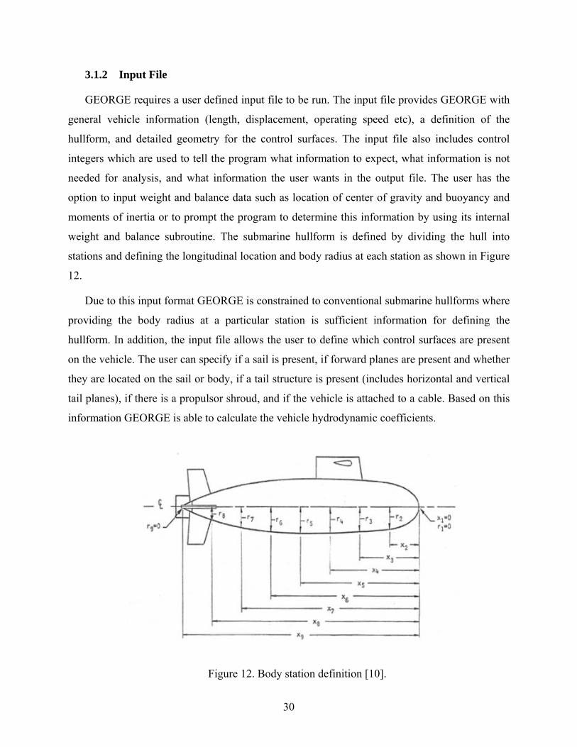
3.1.2 Input File

GEORGE requires a user defined input file to be run. The input file provides GEORGE with

general vehicle information (length, displacement, operating speed etc), a definition of the

hullform, and detailed geometry for the control surfaces. The input file also includes control

integers which are used to tell the program what information to expect, what information is not

needed for analysis, and what information the user wants in the output file. The user has the

option to input weight and balance data such as location of center of gravity and buoyancy and

moments of inertia or to prompt the program to determine this information by using its internal

weight and balance subroutine. The submarine hullform is defined by dividing the hull into

stations and defining the longitudinal location and body radius at each station as shown in Figure

12.

Due to this input format GEORGE is constrained to conventional submarine hullforms where

providing the body radius at a particular station is sufficient information for defining the

hullform. In addition, the input file allows the user to define which control surfaces are present

on the vehicle. The user can specify if a sail is present, if forward planes are present and whether

they are located on the sail or body, if a tail structure is present (includes horizontal and vertical

tail planes), if there is a propulsor shroud, and if the vehicle is attached to a cable. Based on this

information GEORGE is able to calculate the vehicle hydrodynamic coefficients.

Figure 12. Body station definition [10].

30

3.1.3 Program Structure

Figure 13 is a block-diagram representation of the program. It shows that GEORGE consists

of a main program with a number of subroutines embedded in it. The main program reads and

writes the control integers and vehicle input and the weight and balance information. It calculates

and writes the bare hull hydrodynamic information and total wind axis derivatives. It also

computes the body axis derivatives from the wind axis data and writes the total body derivatives.

The subroutine SWTBAL computes the vehicle weight and balance data if not already input

by the user. There is subroutine for each control surface which computes and writes the local

stability derivatives for each specific control surface; SSAIL for the sail, SSFWP for the forward

planes, STAIL for the horizontal and vertical tail planes, and SSHROUD for the propulsor

shroud. The control integers defined in the input file determine which of these subroutines need

to be run. Each control surface subroutine calculates the local hydrodynamic coefficients for its

specific control surface based on geometry and then transforms the local coefficients from the

local axis system to the vehicle axis system. These values of the coefficients are read into the

main program and used in the calculation of the total body coefficients. In addition the SCABLE

subroutine calculates the cable stability derivatives for towed vehicles. The ADDMASS

subroutine computes the component added mass derivatives. The TFLONG and TFLAT

subroutines calculate the longitudinal and lateral hydrodynamic transfer functions and roots of

the characteristic equation respectively.

31

GEORGE Mainline Program

SWBAL

Reads input and computes vehicle weight and balance data

SSFWP

Reads input, computes, and writes fairwater stability

derivatives

STAIL

Reads input, computes, and writes tail stability derivatives

SSHROUD

Reads input, computes, and writes shroud stability derivatives

ADDMASS

Computes and writes component added mass stability derivatives

SCABLE

Reads input, computes, and writes cable stability derivatives

TFLONG

Computes and writes longitudinal hydrodynamic transfer function

coefficients and roots of characteristic equation. Create

timeplot data file

TFLAT

Computes and writes lateral hydrodynamic transfer function

coefficients and roots of characteristic equation. Create

timeplot data file.

SSAIL

Reads input, computes, and writes sail stability derivativesReads and writes

control integers , title and vehicle

information

Reads and writes weight and

balance information

Calculates and writes total wind axis derivatives

Computes body axis derivatives SNAME) from, produces and

writes total body derivatives

Reads all or selected stability

derivatives as specified by

control integers

Reads sensitivity analysis

Produces LOCSAP, LASOP, and part of timeplot data files

GEORGE Mainline Program

SWBAL

Reads input and computes vehicle weight and balance data

SSFWP

Reads input, computes, and writes fairwater stability

derivatives

STAIL

Reads input, computes, and writes tail stability derivatives

SSHROUD

Reads input, computes, and writes shroud stability derivatives

ADDMASS

Computes and writes component added mass stability derivatives

SCABLE

Reads input, computes, and writes cable stability derivatives

TFLONG

Computes and writes longitudinal hydrodynamic transfer function

coefficients and roots of characteristic equation. Create

timeplot data file

TFLAT

Computes and writes lateral hydrodynamic transfer function

coefficients and roots of characteristic equation. Create

timeplot data file.

SSAIL

Reads input, computes, and writes sail stability derivativesReads and writes

control integers , title and vehicle

information

Reads and writes weight and

balance information

Calculates and writes total wind axis derivatives

Computes body axis derivatives SNAME) from, produces and

writes total body derivatives

Reads all or selected stability

derivatives as specified by

control integers

Reads sensitivity analysis

Produces LOCSAP, LASOP, and part of timeplot data files

SWBAL

Reads input and computes vehicle weight and balance data

SSFWP

Reads input, computes, and writes fairwater stability

derivatives

STAIL

Reads input, computes, and writes tail stability derivatives

SSHROUD

Reads input, computes, and writes shroud stability derivatives

ADDMASS

Computes and writes component added mass stability derivatives

SCABLE

Reads input, computes, and writes cable stability derivatives

TFLONG

Computes and writes longitudinal hydrodynamic transfer function

coefficients and roots of characteristic equation. Create

timeplot data file

TFLAT

Computes and writes lateral hydrodynamic transfer function

coefficients and roots of characteristic equation. Create

timeplot data file.

SSAIL

Reads input, computes, and writes sail stability derivatives

SWBAL

Reads input and computes vehicle weight and balance data

SSFWP

Reads input, computes, and writes fairwater stability

derivatives

STAIL

Reads input, computes, and writes tail stability derivatives

SSHROUD

Reads input, computes, and writes shroud stability derivatives

ADDMASS

Computes and writes component added mass stability derivatives

SCABLE

Reads input, computes, and writes cable stability derivatives

TFLONG

Computes and writes longitudinal hydrodynamic transfer function

coefficients and roots of characteristic equation. Create

timeplot data file

TFLAT

Computes and writes lateral hydrodynamic transfer function

coefficients and roots of characteristic equation. Create

timeplot data file.

SSAIL

Reads input, computes, and writes sail stability derivatives

SWBAL

Reads input and computes vehicle weight and balance data

SWBALSWBAL

Reads input and computes vehicle weight and balance data

SSFWP

Reads input, computes, and writes fairwater stability

derivatives

SSFWPSSFWP

Reads input, computes, and writes fairwater stability

derivatives

STAIL

Reads input, computes, and writes tail stability derivatives

STAILSTAIL

Reads input, computes, and writes tail stability derivatives

SSHROUD

Reads input, computes, and writes shroud stability derivatives

SSHROUDSSHROUD

Reads input, computes, and writes shroud stability derivatives

ADDMASS

Computes and writes component added mass stability derivatives

ADDMASSADDMASS

Computes and writes component added mass stability derivatives

SCABLE

Reads input, computes, and writes cable stability derivatives

SCABLESCABLE

Reads input, computes, and writes cable stability derivatives

TFLONG

Computes and writes longitudinal hydrodynamic transfer function

coefficients and roots of characteristic equation. Create

timeplot data file

TFLONGTFLONG

Computes and writes longitudinal hydrodynamic transfer function

coefficients and roots of characteristic equation. Create

timeplot data file

TFLAT

Computes and writes lateral hydrodynamic transfer function

coefficients and roots of characteristic equation. Create

timeplot data file.

TFLATTFLAT

Computes and writes lateral hydrodynamic transfer function

coefficients and roots of characteristic equation. Create

timeplot data file.

SSAIL

Reads input, computes, and writes sail stability derivatives

SSAILSSAIL

Reads input, computes, and writes sail stability derivativesReads and writes

control integers , title and vehicle

information

Reads and writes weight and

balance information

Calculates and writes total wind axis derivatives

Computes body axis derivatives SNAME) from, produces and

writes total body derivatives

Reads all or selected stability

derivatives as specified by

control integers

Reads sensitivity analysis

Produces LOCSAP, LASOP, and part of timeplot data files

Figure 13. GEORGE Flowchart.

3.1.4 Output File

An output file is created each time GEORGE is run. The output file summarizes the

information provided in the input file and provides the desired output information specified in

the input file. Specifically, it details the input control integers, input vehicle information and

hullform shape as well as the input geometry for each control surface specified. The output

includes specific output for each subroutine (mainly the local axis hydrodynamic derivatives for

each control surface) and the main program output. For the scope of this thesis the only output of

interest are the non-dimensional total body hydrodynamic coefficient/derivatives.

3.2 CEBAXI and LA_57

In addition to GEORGE another submarine stability code was used to determine the stability

characteristics of each design. This program is a combination of two codes and is used at the

32

Naval Surface Warfare Center, Carderock Division (NSWCCD) in Bethesda, Maryland by the

Maneuvering and Controls Division of the Hydromechanics Department. These programs are

written in FORTRAN and executed sequentially.

3.2.1 CEBAXI

CEBAXI was initially developed by Tuncer Cebeci in the Mechanical Engineering

Department at California State University at Long Beach in February of 1978. Since 1978 it has

been modified and used by NSWCCD. The program is designed to calculate the incompressible

laminar and turbulent boundary layers on plane and axisymmetric bodies. It requires the hull

offsets non-dimensionalized by the overall length as input and its output is necessary to run the

LA_57 code. CEBAXI requires about 100 stations for the offsets with more stations concentrated

along the nose and tail of the submarine to ensure proper approximations of the boundary layer

and velocity profiles [7].

3.2.2 LA_57

LA_57 was developed in 1994 by the Maneuvering and Controls Division at NSWCCD. It

computes the forces and moments acting on an appended body of revolution. The theory of the

code focuses on a mathematical formulation that contains relevant viscous fluid physics, but is

simple enough for rapid computation. It uses potential flow theory along the hull and lifting line

theory for all appendages. Hull separation is represented by discrete vortices and vortices from

the hull and appendages are tracked and interactions are computed. LA_57 requires less input

than GEORGE. It uses the output from CEBAXI as input and also needs for each control surface

the x-location measured from the nose, span, root chord, and tip chord. This code can model bow

planes, sail planes, a fairwater, and different stern configurations [7].

3.3 Control Surfaces Database

To use GEORGE or CEBAXI and LA_57 to calculate the hydrodynamic coefficients of each

submarine the geometry of the control surfaces needs to be known. Both programs require

detailed information for the fairwater (sail), forward planes, and stern planes. If a fairwater is

present, then GEORGE assumes that the forward planes are attached to the fairwater and

symmetric about the longitudinal axis. Every configuration considered in this thesis has a

fairwater, therefore when GEORGE is used to analyze stability only sail planes will be

33

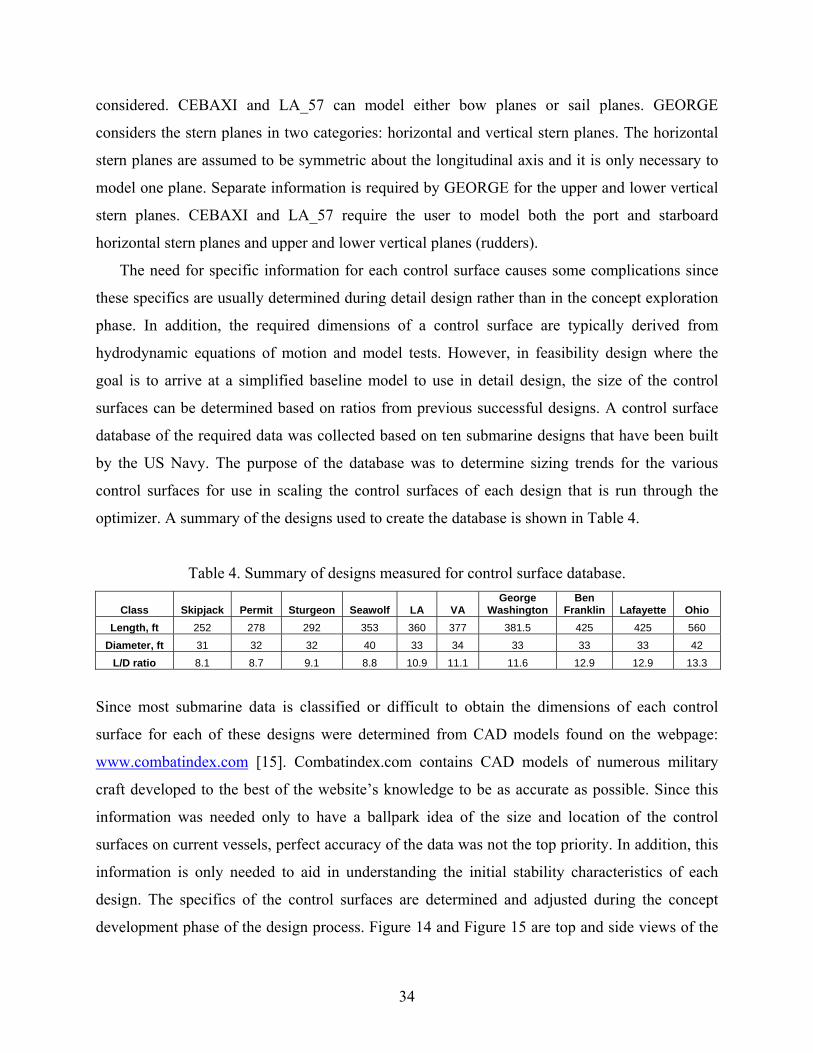
considered. CEBAXI and LA_57 can model either bow planes or sail planes. GEORGE

considers the stern planes in two categories: horizontal and vertical stern planes. The horizontal

stern planes are assumed to be symmetric about the longitudinal axis and it is only necessary to

model one plane. Separate information is required by GEORGE for the upper and lower vertical

stern planes. CEBAXI and LA_57 require the user to model both the port and starboard

horizontal stern planes and upper and lower vertical planes (rudders).

The need for specific information for each control surface causes some complications since

these specifics are usually determined during detail design rather than in the concept exploration

phase. In addition, the required dimensions of a control surface are typically derived from

hydrodynamic equations of motion and model tests. However, in feasibility design where the

goal is to arrive at a simplified baseline model to use in detail design, the size of the control

surfaces can be determined based on ratios from previous successful designs. A control surface

database of the required data was collected based on ten submarine designs that have been built

by the US Navy. The purpose of the database was to determine sizing trends for the various

control surfaces for use in scaling the control surfaces of each design that is run through the

optimizer. A summary of the designs used to create the database is shown in Table 4.

Table 4. Summary of designs measured for control surface database.

Class Skipjack Permit Sturgeon Seawolf LA VA George

Washington Ben

Franklin Lafayette Ohio Length, ft 252 278 292 353 360 377 381.5 425 425 560

Diameter, ft 31 32 32 40 33 34 33 33 33 42 L/D ratio 8.1 8.7 9.1 8.8 10.9 11.1 11.6 12.9 12.9 13.3

Since most submarine data is classified or difficult to obtain the dimensions of each control

surface for each of these designs were determined from CAD models found on the webpage:

www.combatindex.com [15]. Combatindex.com contains CAD models of numerous military

craft developed to the best of the website’s knowledge to be as accurate as possible. Since this

information was needed only to have a ballpark idea of the size and location of the control

surfaces on current vessels, perfect accuracy of the data was not the top priority. In addition, this

information is only needed to aid in understanding the initial stability characteristics of each

design. The specifics of the control surfaces are determined and adjusted during the concept

development phase of the design process. Figure 14 and Figure 15 are top and side views of the

34

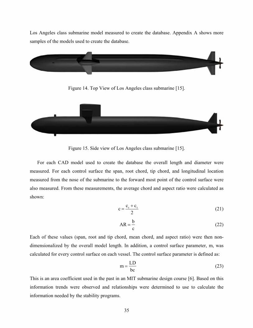
Los Angeles class submarine model measured to create the database. Appendix A shows more

samples of the models used to create the database.

Figure 14. Top View of Los Angeles class submarine [15].

Figure 15. Side view of Los Angeles class submarine [15].

For each CAD model used to create the database the overall length and diameter were

measured. For each control surface the span, root chord, tip chord, and longitudinal location

measured from the nose of the submarine to the forward most point of the control surface were

also measured. From these measurements, the average chord and aspect ratio were calculated as

shown:

2ccc tr += (21)

cbAR = (22)

Each of these values (span, root and tip chord, mean chord, and aspect ratio) were then non-

dimensionalized by the overall model length. In addition, a control surface parameter, m, was

calculated for every control surface on each vessel. The control surface parameter is defined as:

bcLDm = (23)

This is an area coefficient used in the past in an MIT submarine design course [6]. Based on this

information trends were observed and relationships were determined to use to calculate the

information needed by the stability programs.

35

The following sections give detailed information about the specific geometry needed by

GEORGE and CEBAXI and LA_57 for each control surface and a description of the method

used to determine these values.

3.3.1 Forward Planes

This section details the geometry of the forward planes that GEORGE and CEBAXI and

LA_57 require as inputs.

3.3.1.1 GEORGE

Table 5 summarizes the control surface information needed by GEORGE for the forward

planes.

Table 5. Summary of forward plane geometry needed for GEORGE.

Forward Planes Variable Description XNACSA x-location of the aerodynamic center measured from the nose ZACSAL z-location of the aerodynamic center measured from the centerline TRSAL taper ratio BSAL span

BSALQC span measured perpendicular to the body centerline at the aerodynamic center SSAL total planform area of both surfaces

YACSAL y-location of the aerodynamic center ARSAL total aspect ratio of both surfaces

LAMDSA sweep angle in degrees DIHDSA dihedral angle in degrees IDSAL incidence angle in degrees FWDIA fairwater thickness or body diameter at fwd plane quarter chord NTACH attached in a conventional or non-conventional manner CL0SAL zero angle of attack lift coefficient CD0SAL zero angle of attack drag coefficient CM0SAL zero angle of attack moment coefficient

DEDA tail downwash angle with respect to change in vehicle angle of attack DWD tail downwash angle

TOCSAL thickness to chord ratio ANSWER forward planes are fixed or movable

Figure 16 and Figure 17 provide a graphical definition of the forward plane geometry. The z-

location of the aerodynamic center is negative if the aerodynamic center is above the centerline.

Since the forward planes are assumed to be symmetric about the longitudinal axis only one plane

36

is modeled, however, the value provided for the planform area and aspect ratio should be the

value for the two planes combined. For the scope of this thesis the dihedral and incidence angle

is zero. The variable FWDIA is used for the calculations necessary to include the Kb-Kw effect

which accounts for the interference factor between the body and the planes. If FWDIA is set to

zero, the body diameter necessary for the Kb-Kw calculations is determined by the program,

therefore, this value is always set to zero. NTACH refers to the attachment of the forward planes.

Conventional attachment is defined as planes that are attached to the body on the body plane of

symmetry. The forward planes are attached to the sail as shown in Figure 16 and Figure 17 rather

than the body therefore the forward planes are considered to be attached in a non-conventional

way. The forward planes are assumed to be NACA 0020 airfoils. Since this is a symmetric airfoil

the zero angle of attack lift and moment coefficients are always zero and the thickness to chord

ratio is 0.20. The variables DEDA and DWD refer to the velocity field produced by the forward

planes that can affect the angle of attack of any control surfaces aft of the forward planes. Since

only controls fixed stability is considered for the scope of this thesis the angle of attack for every

control surface is set to zero and the downwash has no effect on planes aft of the forward planes,

therefore these variables are always set to zero.

Figure 16. Forward plane attached to fairwater geometry, top view [10].

37

Figure 17. Forward plane attached to fairwater geometry, end view [10].

3.3.1.2 CEBAXI and LA_57 CEBAXI and LA_57 require the x-location, span, root chord, and tip chord of the forward

planes be provided as input. The x-location of the forward planes is measured from the bow of

the submarine. The user can decide if bow planes or sail planes will be modeled. If sail planes

are modeled then the height of the sail planes above the centerline needs to be specified as well

as the information previously noted.

3.3.2 Fairwater Geometry

This section details the fairwater/sail geometry required as inputs by GEORGE and CEBAXI

and LA_57.

3.3.2.1 GEORGE Table 6 summarizes the fairwater geometry needed by GEORGE.

38

Table 6. Summary of fairwater geometry needed for GEORGE.

Fairwater Variable Description XNACFW x-location of the aerodynamic center measured from the nose ZACFWP z-location of the aerodynamic center measured from the centerline TRFWP taper ratio BFWP span

BFWPQC span measured perpendicular to the body centerline at the aerodynamic center SFWP planform area

ARFWP aspect ratio LAMDFW sweep angle in degrees EFFFWP fairwater efficiency XOCHFW x-distance from fairwater leading edge to fwd plane aerodynamic center divided by fairwater

chord at fwd plane aerodynamic center ZOBHFW z-distance from hull to aerodynamic center of fwd plane divided by the exposed span of the

fairwater CL0FWP zero angle of attack lift coefficient CD0FWP zero angle of attack drag coefficient CM0FWP zero angle of attack moment coefficient TOCFWP thickness to chord ratio

Figure 18 and Figure 19 provide a graphical definition of the fairwater geometry. The z-

location of the aerodynamic center is negative if the aerodynamic center is above the centerline.

For the scope of this thesis the dihedral and incidence angle is always zero. The efficiency of the

fairwater is always assumed to be 1. Like the forward planes the fairwater is assumed to be a

NACA 0020 airfoil. Therefore, the zero angle of attack lift and moment coefficients are always

zero and the thickness to chord ratio is 0.20.

Figure 18. Fairwater geometry, side view (bow is to the left) [10].

39

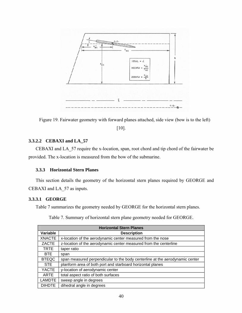
Figure 19. Fairwater geometry with forward planes attached, side view (bow is to the left)

[10].

3.3.2.2 CEBAXI and LA_57 CEBAXI and LA_57 require the x-location, span, root chord and tip chord of the fairwater be

provided. The x-location is measured from the bow of the submarine.

3.3.3 Horizontal Stern Planes

This section details the geometry of the horizontal stern planes required by GEORGE and

CEBAXI and LA_57 as inputs.

3.3.3.1 GEORGE Table 7 summarizes the geometry needed by GEORGE for the horizontal stern planes.

Table 7. Summary of horizontal stern plane geometry needed for GEORGE.

Horizontal Stern Planes Variable Description XNACTE x-location of the aerodynamic center measured from the nose ZACTE z-location of the aerodynamic center measured from the centerline TRTE taper ratio BTE span

BTEQC span measured perpendicular to the body centerline at the aerodynamic center STE planform area of both port and starboard horizontal planes

YACTE y-location of aerodynamic center ARTE total aspect ratio of both surfaces

LAMDTE sweep angle in degrees DIHDTE dihedral angle in degrees

40

Variable Description IDTE incidence angle in degrees

EFFTE horizontal plane efficiency NTACH attached in conventional or non-conventional manner CL0TE zero angle of attack lift coefficient CD0TE zero angle of attack drag coefficient CM0TE zero angle of attack moment coefficient PHITE angle of rotation TOCTE thickness to chord ratio

Figure 20 and Figure 21 provide a graphical definition of the horizontal stern plane

geometry. The z-location of the aerodynamic center is negative if the aerodynamic center is

above the centerline. Since the horizontal planes are assumed to be symmetric about the

longitudinal axis only one plane is modeled however, the value provided for the planform area

and aspect ratio should be the value for the two planes combined. For the scope of this thesis the

dihedral and incidence angle is always zero. The efficiency of the horizontal planes is always

assumed to be one. NTACH refers to whether the horizontal planes are attached in a

conventional or non-conventional manner. Like the forward planes, conventional attachment is

determined as planes that are attached to the body on the body plane of symmetry. Therefore the

horizontal planes are always attached in a conventional manner. The horizontal planes are

assumed to be NACA 0020 airfoils, therefore, the zero angle of attack lift and moment

coefficients are always zero and the thickness to chord ratio is 0.20. The angle Φ is used to

model different stern plane configurations; more detail is provided Section 3.2.4.

41

Figure 20. Horizontal stern plane geometry, top view [10].

Figure 21. Horizontal stern plane geometry, side and end views [10].

3.3.3.2 CEBAXI and LA_57 CEBAXI and LA_57 require that information for both the port and starboard horizontal stern

planes be input. For the purpose of this thesis the geometry of the port and starboard stern planes

are assumed to be identical. The x-location, span, root chord, and tip chord of each plane is

needed as input. The x-location is measured from the bow of the submarine and the span is

measured from the centerline. In addition, the angle of each plane measured from the lower

vertical is also needed. For a cruciform stern configuration the port and starboard planes are

placed at -90 and 90 degrees respectively. Details for an x-stern configuration are provided in

Section 3.3.4.2.

3.3.4 Vertical Stern Planes

This section details the input geometry for the vertical stern planes required by GEORGE and

CEBAXI and LA_57.

42

3.3.4.1 GEORGE

Table 8 provides a summary of the geometry needed by GEORGE for the vertical stern

planes.

Table 8. Summary of geometry for upper and lower vertical stern planes for GEORGE.

Upper Vertical Stern Plane Variable Description XNACUV x-location of the aerodynamic center measured from the nose ZACUVT z-location of the aerodynamic center measured from the centerline TRUVT taper ratio BUVT span

BUVTQC span measured perpendicular to the body centerline at the aerodynamic center SUVT planform area of both port and starboard horizontal planes

ARUVT aspect ratio LAMDUVT sweep angle in degrees EFFUVT efficiency of upper vertical tail CLOVT zero angle of attack lift coefficient CD0VT zero angle of attack drag coefficient

CMOUVT zero angle of attack moment coefficient PHIUVT angle of rotation TOCUVT thickness to chord ratio

Lower Vertical Stern Plane Variable Description XNACLV x-location of the aerodynamic center measured from the nose ZACLVT z-location of the aerodynamic center measured from the centerline TRLVT taper ratio BLVT span

BLVTQC span measured perpendicular to the body centerline at the aerodynamic center SLVT planform area of both port and starboard horizontal planes ARVT aspect ratio

LAMDLV sweep angle in degrees EFFLVT efficiency of lower vertical tail CL0VT zero angle of attack lift coefficient CD0VT zero angle of attack drag coefficient CM0VT zero angle of attack moment coefficient PHILVT angle of rotation TOCLVT thickness to chord ratio

Figure 22 provides a graphical definition of the vertical stern plane geometry. The z-location

of the aerodynamic center is negative if the aerodynamic center is above the centerline. Since it

is typical that the geometry of the upper and lower vertical stern planes not identical due to dry

dock requirements each plane is modeled separately. The efficiency of the vertical stern planes is

always assumed to be one. The vertical stern planes are assumed to be NACA 0020 airfoils,

therefore, the zero angle of attack lift and moment coefficients are always zero and the thickness

to chord ratio is 0.20. The angle Φ is used to model different stern plane configurations. It is 43

local for each plane. When Φ is equal to zero for the vertical and horizontal stern planes the

configuration is as shown in Figure 11. The angle is measured positive counterclockwise. For

this thesis only cruciform and x-stern configurations are considered. Cruciform configurations

are modeled by modeling horizontal planes and both upper and lower vertical planes each with Φ

set to zero. An x-stern is modeled by modeling only the upper and lower vertical planes, each

with phi set to 45 degrees, GEORGE automatically models the other fin across the plane of

symmetry.

Figure 22. Vertical stern plane geometry, side view [10].

3.3.4.2 CEBAXI and LA_57 CEBAXI and LA_57 require that information for both the upper and lower rudders be input.

The x-location, span, root chord, and tip chord of each plane is needed. The x-location is

measured from the bow of the submarine and the span is measured from the centerline. In

addition, the angle of each plane measured from the lower vertical is needed. For a cruciform

stern configuration the upper and lower planes are at 180 and 0 degrees respectively. For an x-

stern configuration the same input is needed however the planes are divided into two categories,

the upper and lower starboard planes and upper and lower port planes. The upper and lower

starboard planes are placed at angles of 135 and 45 degrees respectively and the upper and lower

port planes are places at -135 and -45 degrees respectively. For an x-stern configuration the

geometry for the upper port and starboard planes is equal to the geometry for the upper vertical

44

stern planes needed by GEORGE and the geometry for the lower port and starboard planes is

equal to the geometry for the lower vertical stern plane needed by GEORGE.

3.3.5 General Procedure

This section details the process used to calculate the geometry of the controls surfaces needed

by GEORGE and CEBAXI and LA_57. GEORGE requires more geometry to be input than the

NSWCCD program, therefore the majority of this section refers to GEORGE input variables. It

is indicated when an equation applies to both the input required by GEORGE and CEBAXI and

LA_57. Table 9 summarizes the variables used in this section to calculate the geometry of the

control surfaces.

Table 9. Basic definitions. Basic Definitions

L overall length D diameter c mean chord cr root chord ct tip chord b span

bac span at aerodynamic center AR aspect ratio, AR=b/c Ap projected area, Ap=bc S planform area, S=AR/b² t taper ratio, t=ct/cr

Xac x-location of aerodynamic center measured from the nose Zac z-location of aerodynamic center measured from the centerline Yac y-location of aerodynamic center

Each design in the synthesis model and optimizer is given a unique set of control surfaces.

The geometry of each control surface is dependent on the overall length and diameter of the

design being considered. Given the overall length and diameter of the design, the control surface

parameter, m, for each control surface is determined. Based on the data gained from the ten

submarine designs measured to create the control surface database a plot for each control surface

of the control surface parameter vs. length to diameter ratio was made. These plots are shown as

Figures B1-B5 in Appendix B. In general as the length to diameter ratio increases so does the

control surface parameter. It is assumed that the length to diameter ratio and control surface

parameter are directly proportional and a linear trendline was fit to each set of data. This allows

for the data to be easily extrapolated outside of the length to diameter range for which data was

45

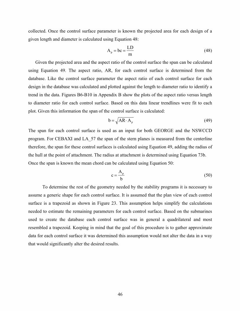
collected. Once the control surface parameter is known the projected area for each design of a

given length and diameter is calculated using Equation 48:

mLDbcAp == (48)

Given the projected area and the aspect ratio of the control surface the span can be calculated

using Equation 49. The aspect ratio, AR, for each control surface is determined from the

database. Like the control surface parameter the aspect ratio of each control surface for each

design in the database was calculated and plotted against the length to diameter ratio to identify a

trend in the data. Figures B6-B10 in Appendix B show the plots of the aspect ratio versus length

to diameter ratio for each control surface. Based on this data linear trendlines were fit to each

plot. Given this information the span of the control surface is calculated:

pAARb ⋅= (49)

The span for each control surface is used as an input for both GEORGE and the NSWCCD

program. For CEBAXI and LA_57 the span of the stern planes is measured from the centerline

therefore, the span for these control surfaces is calculated using Equation 49, adding the radius of

the hull at the point of attachment. The radius at attachment is determined using Equation 73b.

Once the span is known the mean chord can be calculated using Equation 50:

bA

c p= (50)

To determine the rest of the geometry needed by the stability programs it is necessary to

assume a generic shape for each control surface. It is assumed that the plan view of each control

surface is a trapezoid as shown in Figure 23. This assumption helps simplify the calculations

needed to estimate the remaining parameters for each control surface. Based on the submarines

used to create the database each control surface was in general a quadrilateral and most

resembled a trapezoid. Keeping in mind that the goal of this procedure is to gather approximate

data for each control surface it was determined this assumption would not alter the data in a way

that would significantly alter the desired results.

46

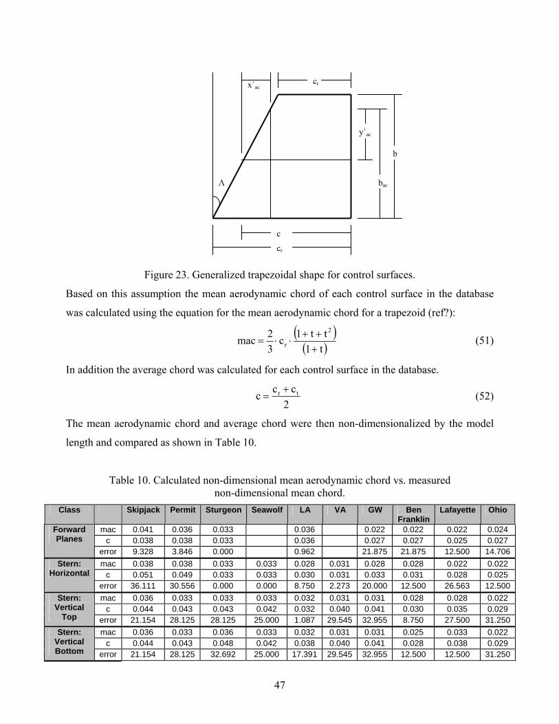
cr

ct

b

bac Λ

c

y`ac

x`ac

Figure 23. Generalized trapezoidal shape for control surfaces.

Based on this assumption the mean aerodynamic chord of each control surface in the database

was calculated using the equation for the mean aerodynamic chord for a trapezoid (ref?):

( )( )t1

tt1c32mac

2

r +++

⋅⋅= (51)

In addition the average chord was calculated for each control surface in the database.

2ccc tr += (52)

The mean aerodynamic chord and average chord were then non-dimensionalized by the model

length and compared as shown in Table 10.

Table 10. Calculated non-dimensional mean aerodynamic chord vs. measured non-dimensional mean chord.

Class Skipjack Permit Sturgeon Seawolf LA VA GW Ben Franklin

Lafayette Ohio

mac 0.041 0.036 0.033 0.036 0.022 0.022 0.022 0.024 c 0.038 0.038 0.033 0.036 0.027 0.027 0.025 0.027

Forward Planes

error 9.328 3.846 0.000 0.962 21.875 21.875 12.500 14.706 mac 0.038 0.038 0.033 0.033 0.028 0.031 0.028 0.028 0.022 0.022

c 0.051 0.049 0.033 0.033 0.030 0.031 0.033 0.031 0.028 0.025 Stern:

Horizontal error 36.111 30.556 0.000 0.000 8.750 2.273 20.000 12.500 26.563 12.500 mac 0.036 0.033 0.033 0.033 0.032 0.031 0.031 0.028 0.028 0.022

c 0.044 0.043 0.043 0.042 0.032 0.040 0.041 0.030 0.035 0.029 Stern:

Vertical Top error 21.154 28.125 28.125 25.000 1.087 29.545 32.955 8.750 27.500 31.250

mac 0.036 0.033 0.036 0.033 0.032 0.031 0.031 0.025 0.033 0.022 c 0.044 0.043 0.048 0.042 0.038 0.040 0.041 0.028 0.038 0.029

Stern: Vertical Bottom error 21.154 28.125 32.692 25.000 17.391 29.545 32.955 12.500 12.500 31.250

47

Data is not given for the forward planes for the Seawolf and Virginia Class submarines because

easurements taken from the ten designs for the database the delta chord,

defined

t −=

these designs had bow planes attached to the body rather than the sail and were therefore,

rectangular rather than trapezoidal. From this data it was determined that the average chord is a

reasonable approximation of the mean aerodynamic chord. This approximation is necessary to

simplify the method used to determine the root and tip chord of the control surfaces for each

design.

Based on the m

as the absolute value of the difference between the measured root and tip chord, was

calculated. These values were non-dimensionalized by the length of the model and then plotted

for each control surface against the length to diameter ratio to determine any trends. These plots

are shown in Figures B11-B15 in Appendix B. Linear trendlines are fit to the data and used to

determine the delta chord value for each specific control surface for a given design. Figure B11,

which shows the data for the forward plane only includes the designs in which the forward

planes are attached to the sail. When the forward planes are attached to the body, the shape of the

control surface is a rectangle as noted earlier, therefore, the root and tip chord are equal to the

mean chord calculated using Equation 52. By assuming the mean aerodynamic chord is equal to

the average chord the root and tip chord can be calculated from the delta chord as follows:

cΔchordcr

cΔchordc+=

(53)

The root chord and tip chord calculated using Equation 53 are used as an input for both

GEORGE and CEBAXI and LA_57. From this information the taper ratio is determined,

t

rct = (54) c

The planform area is determined using the equation for the area of a trapezoid,

)c(cb1S +⋅= 2 tr (55)

The sweep angle, defined as lambda in Figure 23, is determined by the equation,

⎟⎠⎞

⎜⎛ −

= − cctanΛ rr1 (56) ⎝ b

Referring to Figure 23 the variable x`ac is the local x-distance from the leading edge of the

control surface to its aerodynamic center. This distance can be determined using the low speed,

thin airfoil approximation that the aerodynamic center is at quarter mean aerodynamic chord,

48

c0.25x'ac ⋅= (57)

The variable acy' is the local y distance from the aerodynamic center to where it intersects the

perimeter of the control surface (refer to Figure 23). This distance is calculated as:

( )Λtany'ac = (58)

Since it is assumed that the mean aerodynamic chord is equal to the mean chord th

x'ac

en the span at

the aerodynamic center is a function of the local y-distance and overall span:

0.5by'b acac += (59)

Information about the overall x and z location of

tion, defined as Zac is measured from the centerline. The overall x-

location

esi

If the value of bac is greater than b, then is it assumed that the span at the aerodynamic center is

equal to the overall span.

the aerodynamic center for each control

surface is also needed. The x location, defined as Xac, is measured from the nose of the

submarine and the z loca

of the aerodynamic center is a function of the local x-distance, acx' determined from

Equation 57 and the distance from the nose of the submarine to the forward most point of the

control surface. The database was used to determine the x-distance of each control surface

measured from the nose of the submarine which is denoted as x. For each d gn in the database

the distance x was measured and non-dimensionalized by the length. Table 11 shows the non-

dimensional average location of each control surface measured from the nose of the vessel to the

most forward point of the control surface. The distance x for each control surface varies whether

or not sail or bow planes are present. For GEORGE only cases with sail planes are analyzed.

CEBAXI and LA_57 can model either sail or bow planes.

Table 11. Non-Dimensional x-distance measured from vessel nose.

Non-Dimensional X-Distance measured from nose Sail Planes Bow Planes Forward Plane 0.25 0.14 Horizon tal Tail 0.92 0.90Vertical Tail - Top 0.92 0.90 Vertical Tail - Bot 0.90 tom 0.92 Sail 0.24 0.24 Stern Plane x-location of 1/2c 0.95 0.93

Therefore, the equation used to determine the overall x-locat the aerodyna enter is: ion of mic c

( )ccx'xLX racac −++= (60)

49

CEBAXI and LA_57 only need to know the x-location of the control surfaces measured from the

11

and the length of the submarine. In addition, CEBAXI and

bow of the submarine which is simply the product of the non-dimensional x given in Table

LA_57 need to know the non-

dimensional location of half chord of the stern planes which is also given in the last row of Table

11. These values were determined using data from the database created. The location is used in

the CEBAXI program to generate the velocity profiles necessary for the boundary layer

predictions.

The overall z-location of the aerodynamic center measured from the centerline for the

fairwater and sail planes is:

fairwaterac b0.5D0.5Z ⋅+⋅= (61)

The z-l

ater at 50% of the fairwater span. There was no consensus from the

designs used for the database as to where on the fairwater the

ocation of the fairwater and sail planes is the same because it is assumed that the sail

planes are placed on the fairw

sail planes are placed, therefore,

50% of the fairwater span was assumed. Typically, this location would be determined in part by

the equipment that is placed in the fairwater, therefore it was determined that this generalization

would not significantly affect the intended results of this study.

When sail planes are present and CEBAXI and LA_57 is being used then the height of

the sail planes measured from the centerline is needed. This height is calculated using Equation

62:

fairwatersailplane 0.50b2DZ += (62)

Since the horizontal stern planes are always located on the centerline the overall z-

location for the horizontal planes is always zero. The z-location of the vertical stern planes is

dependent on the radius of the submarine at their location of a

is deter

ttachment. The radius at this point

mined by the equation:

vertical

n

a

aac 0.5b

Lx1D0.5Z

a

+⎟⎟

⎠

⎞

⎜⎜

⎝

⎛⎟⎟⎠

⎞⎜⎜⎝

⎛−⋅⋅= (63)

The span, b, in this equation is the span of the upper or lower vertical stern plane. La is the length

of the aft portion of the submarine, na describes the fullness of the aft portion, and x is defined in

Figure 24. A more detailed explanation of La and na is found in Section 3.3.

The y-location of the aerodynamic center is only required for the forward planes and

horizontal stern planes. As shown in Figure 16 for the forward planes Yac is defined by:

a

50

forwardac 0.5b2tY += (64)

The span, b, is the span of the forward planes and t is the thickness of the fairwater which is

determ

s the z-

location for the vertical stern planes. It is a function of the radius of the submarine at attachment

and the span of the control surface.

ined from the thickness to chord ratio.

The y-location of the horizontal planes is determined in the same manner a

horizontal

n

acx1D0.5Y

a

⎟⎞

⎜⎜

⎝

⎛ ⎞⎛−⋅⋅=

a

a 0.5bL

+⎟⎠

⎟⎟⎠

⎜⎜⎝

(65)

Finally, as shown in Figure 19 some ratios involving distances in reference to the placement

of the forward planes on the fairwater are also needed by GEORGE. XOCHFW is defined in

Figure 19 as

ac

ac

cx'

The

(66)

variable cac is the mean chord of the fairwater which is determined using Equation 52 and

acx' is calculated as:

sailrsailforwardac,ac c)(cxXx' −−−= (67)

Where is the overall x-location of the

Tab d c are properties of the fairwater. The variable ZOBHFW is defined in

Figure 19 as:

forwardac,X forward planes determined in Equation 60, sailx

is the x-location of the forward most point of the sail measured from the nose (determined using

le 11), and cr an

bzac 68)

ations are implemented in a FORTRAN code (ControlSurfaces.f90) so the

geometry of the control surfaces can be quickly determined for any given diameter, length to

diameter ratio, plane configuration, and stern configuration.

(

Zac in this equation is defined as the vertical distance from the base of the fairwater to the mean

chord which is defined 0.5bfairwater and b is the span of the fairwater.

These equ

51

3.4 Hull Offsets

In addition to the geometry of the control surfaces GEORGE and CEBAXI and LA_57

require the hull offsets to calculate the hydrodynamic coefficients. A traditional teardrop shape

ed for the hullform. This idealized shape was chosen for its low submerged resistance

and l bow and parabolic stern as shown in Figure 24. The teardrop shape

can

was assum

consists of an elliptica

be modified to include a section of parallel midbody as needed as also shown in Figure 24.

The aft body is idealized as parabolic and La represents the length of the aft body while the nose

is assumed to be elliptical and Lf represents its length. La and Lf are determined from the

diameter as follows:

2.4DL3.6DL

f

a

==

(69)

The overall length, L, is determined from the diameter and length to diameter ratio,

DLDL ⋅= (70)

The length of the parallel midbody, Lpmb is a function of the overall length and length of the fore

pmb

and aft bodies:

(LLL )Lfa− += (71)

The hullform is defined by specifying 45 stations along the nose from the most forward point

to the beginning of the parallel midbody section and by defining 45 stations along the stern from

the end of the parallel midbody section to the aft most point of the vessel. Each station is defined

by an x-distance measured from the bow and z-distance (r

The

adius) measured from the centerline.

x-location for the fore and aft bodies is determined as follows:

1ia,a

ia,

1if,f

if,

X10LX

X10LX

−

−

+=

+= (72a, 72b)

The index i varies from 1 to 39 for the forward body, Xf,40 is always equal to 0.5D. The index i

for the aft body varies from 2 to 40 and Xa,1 is always equal to 0.5D. The radius for each station

is determined using Equations 72a and 72b:

52

⎥⎥⎦

⎤

⎢⎢⎣

⎡⎟⎟⎠

⎞⎜⎜⎝

⎛ +−−=

⎥⎥⎤

⎢⎢⎣

⎡⎟⎟⎞

⎜⎜⎝

⎛ −−=

ff n1

nif,f

if, LxL

12DZ

⎦⎠

an

a

pmbfia,ia,

f

L)L(Lx

12DZ

(73a, 73b)

In this equation nf and na determine the fullness of the nose

variables are used to indicate how quickly and at what slope the nose and stern taper to a point.

These equations are implemented in a FORTRAN code (HullOffsets.f90) to determine the

and stern respectively. These

offsets of any hullform defined by a diameter, length to diameter ratio, and the fullness

exponents of the bow and stern.

Figure 24. Teardrop and modified teardrop hullform [4].

53

CHAPTER 4 RESPONSE SURFACE MODEL (RSM) TOOLS

Response surface models are used to predict the behavior of response/output variables for a

given set of input/design variables. Experimental data is used to develop a parametric equation to

represent the response. This chapter summarizes the tools used to build the response surface

models (RSMs). The first part of the chapter describes the tools used to automate the process of

varying the inputs of GEORGE and CEBAXI and LA_57 (control surface geometry and hull

offsets) to analyze their affect on the horizontal and vertical stability indices. ModelCenter is the

main tool used however there are different plug-ins and tools utilized within the program which

are described in more detail in the following sections. The second part of the chapter describes

the process of integrating the stability programs and the control surfaces and hull offsets

programs into the ModelCenter environment to perform the analysis.

4.1 Tools For Analysis

4.1.1 ModelCenter

ModelCenter is a visual environment for process integration developed by Phoenix

Integration. It provides a means to link a number of design applications in one environment that

allows for the sharing of input and output variables. It automates the process by providing tools

for wrapping analysis programs, performing trade studies and optimizations, visualizing the

design space, performing response surface modeling, developing parametric models of the

design space, and archiving the results. This in turn reduces error, saves time, and produces more

efficient designs [14].

Figure 25 shows an example of the ModelCenter environment. The server browser is located

at the bottom and displays the components that can be added to the model which are added by

clicking and dragging the component into the workspace. The workspace is represented by the

area with the blue background. The component tree, displayed on the left, lists each component

in the model, which are represented in the workspace by each box. Each component can be

opened in the component tree to show the individual inputs and outputs associated with it.

54

Figure 25. Example of ModelCenter environment.

4.1.2 Analysis Server

ModelCenter cannot be run without Analysis Server. Analysis server allows the user to wrap

analysis software into usable components. Common programs such as FORTRAN codes, Excel

spreadsheets, MATLAB m-files, and MATHCAD files can be wrapped using this tool. The

purpose of wrapping a program is to convert program-specific input and output operations into a

generic set of commands. The process of wrapping a program is discussed in more detail in

Section 4.2.1. By wrapping a program, the process of manually creating individual input files

necessary to run programs such as FORTRAN codes which require specific input files, is

eliminated. This in turn speeds up the process of analyzing a variety of different input

combinations and automates the process, leaving the user free to focus on the results.

4.1.3 Design of Experiments Toolkit

The design of experiments (DOE) tool simplifies the process of varying input/design

variables to observe the corresponding affect on the output/response variables. A range is defined

for each design variable and each point in the range defines a design point. The DOE tool selects

55

specific design points and documents the responses of the model at those chosen design points

[14]. Figure 26 shows the DOE graphical interface in ModelCenter.

To perform a DOE the design variables and response variables need to be specified. This can

be done by dragging them from the component tree into the DOE window. For each design

variable a design range is defined by specifying high and low boundaries. The next step is to

select a DOE algorithm to be used. The algorithm is selected based on the desired purpose of the

experiment. Some algorithms are selected to test a design for robustness by determining the

extent to which the designs in the specified design space are feasible. Other algorithms are used

to define a design variable’s effect on one another while others are selected to screen a large

number of design variables to isolate those that have the greatest effect on the response variables.

The DOE algorithms available are:

• Half Fractional Factorial • Eighth Fractional Factorial • Sixteenth Fractional Factorial • Foldover • Plackett-Burman • Parameter Scan • Full Factorial • Latin-Hypercube • Central Composite • Face Centered Central Composite • Box-Behnken

The half fractional factorial, eight fractional factorial, sixteenth fractional factorial,

foldover, and Plackett-Burman designs are all screening experiments. Screening experiments are

defined as experiments that are used to identify the most active variables and are most useful

when a large number of variables are present.

The parameter scan and full factorial algorithms sample the entire design space. The

parameter scan is limited to testing the high and low levels of each variable while the full

factorial algorithm allows for more levels of each variable to be tested.

The Latin-Hypercube algorithm is the design used for analysis in this thesis. It is similar

to the full factorial design in that it explores the entire design space but does so by taking a

random sample of the entire design space. It does this by dividing the internal space into

segments to achieve a more thorough investigation of the design space. The number of segments

56

and how many random combinations of variables and segments is determined by the specified

number of designs. Once a DOE algorithm is selected the number of runs is specified which

corresponds to the number of data sets to be collected [8].

Figure 26. DOE Tool.

4.1.4 Response Surface Model (RSM) Toolkit

The RSM toolkit is used to create approximations of long running or complex models. The

resulting RSM has a runtime that is much faster than the model it approximates making it more

practical for use with optimization tools which can require thousands of iterations and

evaluations of various functions [14].

The RSM toolkit uses the data generated by the DOE tool and is launched from the DOE

toolbar once the DOE is complete. It allows the user to select which data sets collected by the

DOE will be used to form the response surface. The response surface can then be modeled using

several polynomial options:

57

• Stepwise Regression Quadratic

• Stepwise Regression Cubic

• Linear

• Linear plus Quadratic Interaction Terms

• Full Quadratic

• Linear plus Quadratic and Cubic Interaction Terms

• Full Cubic After the RSM is generated statistical details of the response surface and graphs can be

viewed to determine if the polynomial model chosen is a good fit. It is important to note

however, that a statistical report that describes the resulting RSM as a good fit does not

necessarily mean it is a good fit to the parent model. The resulting RSM is just an approximation

of the actual response and the fit is dependent on the efficiency and sufficiency of the DOE.

Therefore it is important that the appropriate DOE algorithm and sample size is chosen. The

purpose of the RSM is to reduce computational time therefore large DOE sample sizes can be

self-defeating and the DOE algorithm chosen should sufficiently represent the entire design

space [8]. The user can create a number of different response surfaces and determine which gives

the best fit. Once an appropriate RSM is chosen it can be returned to the ModelCenter workspace

either as a module or to replace the parent model it was derived from.

4.1.5 Darwin Optimizer

Darwin is a genetic-algorithm-based trade study designed specifically for engineering

optimization problems. Genetic algorithms are probability based and use processes analogous to

natural selection to search for and determine the best designs. They can be used to solve design

problems with both discrete and continuous design variables and any number of constraints.

They can also be used to perform the Multi-Objective Genetic Optimization described in Section

1.2.4. Darwin allows the user to choose which design variables are used in the optimization and

to specify the constraints. The use of the Darwin optimizer in this thesis will be described in

more detail in Section 6.4.

4.2 Implementation of Dynamic Stability Modules in ModelCenter

This section describes the process of integrating the tools outlined in Chapter 3 into the

ModelCenter environment. Both GEORGE and CEBAXI and LA_57 require input files that

58

specify the hull offsets of the submarine and the geometry of the control surfaces. Individual

FORTRAN codes were written to determine the offsets (HullOffsets.f90) and control surface

geometry (ControlSurfaces.f90) based on a given diameter and length to diameter ratio as

described in Sections 3.4 and 3.3. An additional FORTRAN code (StabilityIndices.f90) was

written to be used with GEORGE to calculate the stability indices derived in Chapter 2 based on

the hydrodynamic coefficients output by GEORGE. These programs represent the individual

components of the models that are created in ModelCenter. Two separate dynamic stability

models are created; one using GEORGE and the one using CEBAXI and LA_57.

4.2.1 Creating a File Wrapper

ModelCenter requires each component to be “wrapped” using a file wrapper. A file wrapper

is useful for programs that require input and output files. Typically, an input/output based

program requires the user to manually modify the input file, run the executable, and extract

pertinent data from the output file each time the program is run. A file wrapper automates this

process by using a simple set of commands to modify an input file, run the executable, and

search the output file each time the component is executed.

A wrapper consists of four sections: header, run command, input file, and output file. Figure

27 shows an example of a file wrapper. The header section documents the wrapper through a

series of comment lines denoted by the symbol #. The run commands section communicates

instructions to run the component. The command “generate inputFile” tells the component to

create the input file necessary to run the executable. Run “HullOffsets.exe” tells ModelCenter

which executable file to run. The command “parse outputFile” prompts ModelCenter to search

the resulting output file for specific output variables. These output variables become part of the

design space in ModelCenter and are made available to other components in the model.

The Input File section prompts an input template file to be opened and then generates a new

input file by replacing specified variables with new values. The section begins with the

command “RowFieldInputFile.” This command defines the structure of the input file stating that

each line is considered a row and each row is comprised of fields. The command “setdelimeters”

specifies what separates the fields in a given row. The default setting is white space however

commas and columns can also be used as delimiters. The variables that are replaced in the

template file to create the new input file are determined by specifying the variable type (double,

59

integer, string, etc) and its location in the input file by specifying its row and field. Therefore the

line:

variable: XNACSA double 35 1 states that the variable XNACSA is type double and located in the input file on row 35, field 1.

The output file section is similar to the input file section. It contains instructions on how

to retrieve values from an output file. The command fileToParse specifies the output file to be

opened and searches it for specific outputs. Like the input file the structure of the output file is

specified by the command “RowFieldOutputFile” and the command “setdelimiters” can be used

to set what separates the individual fields. For components that have particularly large output

files and only a few outputs are desired commands such as “MarkAsBeginning” can be used to

mark a specific place in the output file to begin the search. Variables that are specified in a

wrapper as an output are then available to all components in the model to be used as inputs. This

allows for the different components of each model to be linked together.

Header

Run Commands

Input File

Output File

Figure 27. Example of file wrapper. 60

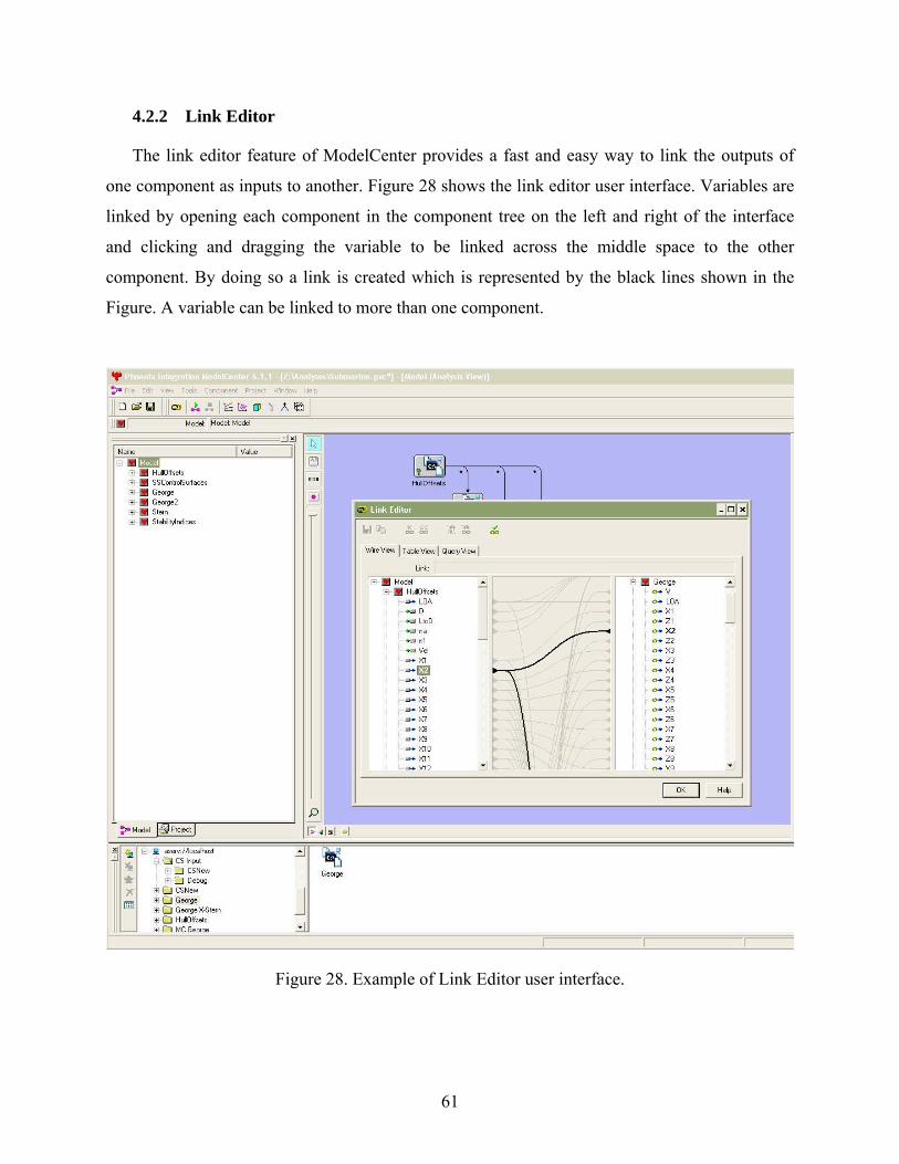
4.2.2 Link Editor

The link editor feature of ModelCenter provides a fast and easy way to link the outputs of

one component as inputs to another. Figure 28 shows the link editor user interface. Variables are

linked by opening each component in the component tree on the left and right of the interface

and clicking and dragging the variable to be linked across the middle space to the other

component. By doing so a link is created which is represented by the black lines shown in the

Figure. A variable can be linked to more than one component.

Figure 28. Example of Link Editor user interface.

61

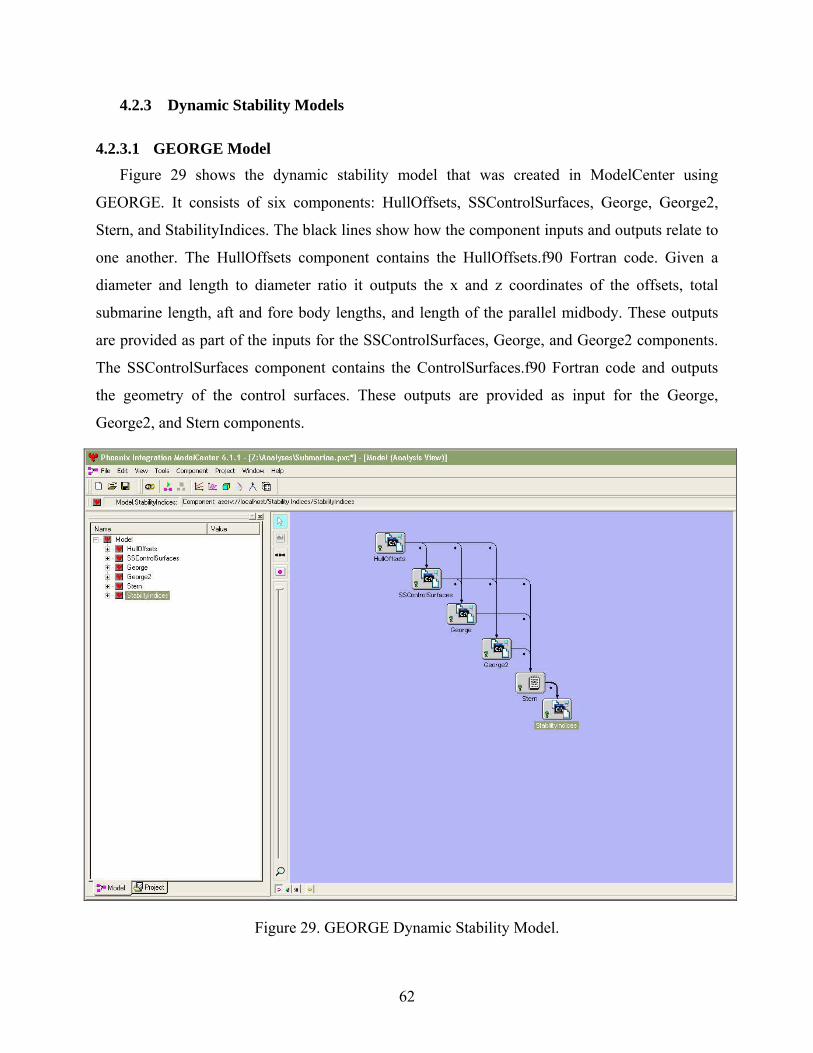
4.2.3 Dynamic Stability Models

4.2.3.1 GEORGE Model Figure 29 shows the dynamic stability model that was created in ModelCenter using

GEORGE. It consists of six components: HullOffsets, SSControlSurfaces, George, George2,

Stern, and StabilityIndices. The black lines show how the component inputs and outputs relate to

one another. The HullOffsets component contains the HullOffsets.f90 Fortran code. Given a

diameter and length to diameter ratio it outputs the x and z coordinates of the offsets, total

submarine length, aft and fore body lengths, and length of the parallel midbody. These outputs

are provided as part of the inputs for the SSControlSurfaces, George, and George2 components.

The SSControlSurfaces component contains the ControlSurfaces.f90 Fortran code and outputs

the geometry of the control surfaces. These outputs are provided as input for the George,

George2, and Stern components.

Figure 29. GEORGE Dynamic Stability Model.

62

There are two George components because each one represents a different stern

configuration. The component George calculates the hydrodynamic coefficients assuming a

cruciform stern configuration while George2 assumes an x-stern. When an x-stern is assumed

only the vertical stern planes are modeled as described in section 3.2.4. There is a component for

each stern configuration because the structure of the input file differs for each configuration. The

stern configuration for the design is denoted by the variable stern which is specified as an input

in the SSControlSurfaces component. If the variable stern has a value of 1 then an x-stern

configuration is assumed, if variable stern is equal to zero then a cruciform stern is assumed.

Both components, George and George2 are executed for each design and each output the

hydrodynamic coefficients that are part of the stability indices. The coefficients output from the

component George are marked by a subscript A and the coefficients output from George2 are

marked with a subscript B. The component Stern determines which set of the hydrodynamic

coefficients, A or B, are provided as inputs to the StabilityIndices component based on the value

of the variable stern which is provided as an input.

StabilityIndices is the final component of the model. It inputs the hydrodynamic coefficients

from the component Stern and calculates the value of the horizontal and vertical stability indices

using Equations 25 and 47. These outputs represent the response variables that are analyzed

using the DOE tool described in section 4.1.3.

4.2.3.2 CEBAXI and LA_57 Model Figure 30 shows the CEBAXI and LA_57 stability model. It consists of three components:

HullOffsets, SSControlSurfaces, and Stability. The HullOffsets and SSControlSurfaces

components are the same components used in the George Dynamic Stability model. The

component stability includes the CEBAXI and LA_57 programs that calculate the stability

indices. The output of the HullOffsets component is part of the input to the SSControlSurfaces

and Stability component. The output of the SSControlSurfaces component is provided as input

for the Stability component.

The CEBAXI and LA_57 model can model bow planes or sail planes and an x-stern or

cruciform stern. Therefore, in total there are four different configurations that can be analyzed:

sail planes with an x-stern, sail planes with a cruciform stern, bow planes with an x-stern, and

bow planes with a cruciform stern. This is done by setting the input variables STERN and

BOWPLANES to either zero or one. If STERN is equal to zero then a cruciform stern is

63

assumed, if it is equal to one then an x-stern is modeled. If BOWPLANES is equal to zero then

sail planes are modeled and if it is equal to one then bow planes are assumed.

Figure 30. NSWCCD Dynamic Stability Model.

64

CHAPTER 5 DESIGN OF EXPERIMENTS RESULTS AND RESPONSE SURFACE MODELS

5.1 GEORGE Dynamic Stability Model

Two separate designs of experiments were performed using the GEORGE dynamic stability

model, one for a cruciform stern configuration and one for an x-stern configuration. Both

configurations had sail planes. Based on the DOE performed response surfaces were created for

each configuration. The resulting plots from the GEORGE DOE performed and RSMs created

are provided in Appendix C. For each DOE performed the Latin-Hypercube algorithm was

chosen to ensure sufficient exploration of the entire design space and the number of runs was set

to 200. Five input/design variables were examined: length to diameter ratio, diameter, aft body

fullness factor, forward body fullness factor, and velocity. Table 12 shows the design variables

and the low and high bounds used for the DOE. The horizontal and vertical stability indices, GH

and GV, were the output/response variables examined. Once a DOE was complete the data

collected was analyzed and any outlying data sets were discarded. Outliers were determined as

data sets with values that were significantly outside of the general trend of the response

variables. The modified data sets were then used to create corresponding response surfaces. The

following sections detail the results of the DOE and RSMs.

Table 12. DOE variables and high and low boundaries for GEORGE stability model.

Design Variable Low High L/D 6.5 13

D (ft) 22 32 na 2.5 3.5 nf 2 3

Velocity (knots) 10 25

5.1.1 Configuration 1: Cruciform Stern

Figure 31 and Figure 32 are plots of the main effects for the horizontal and vertical

stability indices which demonstrate the sensitivity of the output variables to the input variables.

A main effect is defined as the change in a response/output variable with respect to a

design/input variable. It is determined by taking the average output value for a given input

variable at its upper and lower bounds. The main effect is the difference between the two

averages. The variable with the largest main effect has the most influence on the response

65

variable [14]. Therefore, Figure 31 and Figure 32 show that the length to diameter ratio, velocity

and the forward body fullness factor variables have almost an equal influence on both stability

indices.

Figure 31. GH main effects plot for GEORGE model with cruciform stern.

Figure 32. GV main effects plot for GEORGE model with cruciform stern.

Figure 33 plots the stability indices as a function the length to diameter ratio. In general,

as the length to diameter ratio increases the stability increases, however there is a discontinuity

that occurs near a length to diameter ratio of 10 for GH and 10.4 for Gv. At this length to diameter

66

ratio the stability indices increase dramatically over a small range of length to diameter ratios

creating a sharp upward slope in the data. Designs below this length to diameter ratio are highly

unstable while designs above this length to diameter ratio are highly stable.

Figure 33. Stability indices vs.L/D for GEORGE model with cruciform stern

Figure 34 and Figure 35 are variable influence plots. The variable influence plots show

both the main effects as well as the interaction effects of the design variables. Higher order

effects involve more than two variables and are grouped together into one category. The other

category includes variables with an importance less than 0.5% [14]. Therefore, Figure 34 and

Figure 35 show that the length to diameter ratio has the greatest effect on the stability indices for

this configuration and that the higher order terms also have a significant impact.

67

Figure 34. GH variable influence for GEORGE model with a cruciform stern.

Figure 35. GV variable influence for GEORGE model with a cruciform stern.

68

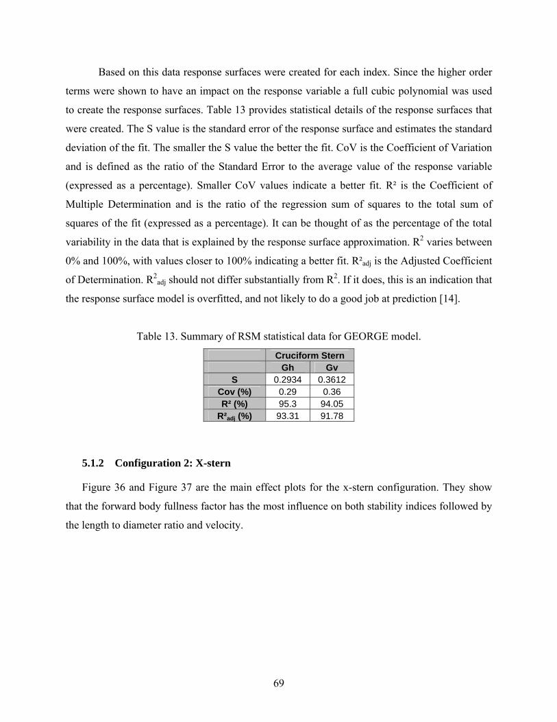
Based on this data response surfaces were created for each index. Since the higher order

terms were shown to have an impact on the response variable a full cubic polynomial was used

to create the response surfaces. Table 13 provides statistical details of the response surfaces that

were created. The S value is the standard error of the response surface and estimates the standard

deviation of the fit. The smaller the S value the better the fit. CoV is the Coefficient of Variation

and is defined as the ratio of the Standard Error to the average value of the response variable

(expressed as a percentage). Smaller CoV values indicate a better fit. R² is the Coefficient of

Multiple Determination and is the ratio of the regression sum of squares to the total sum of

squares of the fit (expressed as a percentage). It can be thought of as the percentage of the total

variability in the data that is explained by the response surface approximation. R2 varies between

0% and 100%, with values closer to 100% indicating a better fit. R²adj is the Adjusted Coefficient

of Determination. R2adj should not differ substantially from R2. If it does, this is an indication that

the response surface model is overfitted, and not likely to do a good job at prediction [14].

Table 13. Summary of RSM statistical data for GEORGE model.

Cruciform Stern Gh Gv

S 0.2934 0.3612 Cov (%) 0.29 0.36 R² (%) 95.3 94.05

R²adj (%) 93.31 91.78

5.1.2 Configuration 2: X-stern

Figure 36 and Figure 37 are the main effect plots for the x-stern configuration. They show

that the forward body fullness factor has the most influence on both stability indices followed by

the length to diameter ratio and velocity.

69

Figure 36. Gh main effects for GEORGE model with an x-stern.

Figure 37. Gv main effects for GEORGE model with an x-stern.

70

Figure 38 shows the stability indices as a function of the length to diameter ratio. The

stability indices increase with increasing length to diameter ratios. However, a discontinuity

occurs at a length to diameter ratio of approximately 10 for both indices. At this length to

diameter ratio the stability indices quickly increase over a small range of length to diameter

ratios. Designs below a length to diameter ratio of 10 are unstable while designs with a length to

diameter ratio greater than 10 are stable. The values of the stability indices tend to converge as

the length to diameter ratio increases from 6.5 to 10 and begin to diverge as the length to

diameter ratio increases from 10 to 13. In addition, the values of horizontal and vertical indices

are closely coupled at higher length to diameter ratios.

Figure 38. Stability indices vs. L/D for GEORGE model with an x-stern.

The variable influence plots shown in Figure 39 and Figure 40 indicate that the length to

diameter ratio has the greatest effect on the indices and shows that the higher order terms are also

important. Since the higher order terms are significant a full cubic polynomial was used to

develop the response surfaces for both indices. Table 14 shows the statistical details of the

response surfaces.

71

Figure 39. Gh variable influence for GEORGE model with an x-stern.

Figure 40. Gv variable influence for GEORGE model with an x-stern.

72

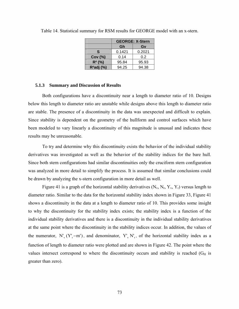
Table 14. Statistical summary for RSM results for GEORGE model with an x-stern.

GEORGE: X-Stern Gh Gv

S 0.1421 0.2021 Cov (%) 0.14 0.2 R² (%) 95.84 95.93

R²adj (%) 94.25 94.38

5.1.3 Summary and Discussion of Results

Both configurations have a discontinuity near a length to diameter ratio of 10. Designs

below this length to diameter ratio are unstable while designs above this length to diameter ratio

are stable. The presence of a discontinuity in the data was unexpected and difficult to explain.

Since stability is dependent on the geometry of the hullform and control surfaces which have

been modeled to vary linearly a discontinuity of this magnitude is unusual and indicates these

results may be unreasonable.

To try and determine why this discontinuity exists the behavior of the individual stability

derivatives was investigated as well as the behavior of the stability indices for the bare hull.

Since both stern configurations had similar discontinuities only the cruciform stern configuration

was analyzed in more detail to simplify the process. It is assumed that similar conclusions could

be drawn by analyzing the x-stern configuration in more detail as well.

Figure 41 is a graph of the horizontal stability derivatives (Nv, Nr, Yv, Yr) versus length to

diameter ratio. Similar to the data for the horizontal stability index shown in Figure 33, Figure 41

shows a discontinuity in the data at a length to diameter ratio of 10. This provides some insight

to why the discontinuity for the stability index exists; the stability index is a function of the

individual stability derivatives and there is a discontinuity in the individual stability derivatives

at the same point where the discontinuity in the stability indices occur. In addition, the values of

the numerator, , and denominator, , of the horizontal stability index as a

function of length to diameter ratio were plotted and are shown in

)m'(Y'N' rv − rv N'Y'

Figure 42. The point where the

values intersect correspond to where the discontinuity occurs and stability is reached (GH is

greater than zero).

73

Figure 41. Horizontal plane stability derivatives vs. L/D.

Horizontal Stability Index

-0.0001

0

0.0001

0.0002

0.0003

0.0004

0.0005

6 7 8 9 10 11 12 13 14

L/D

DenominatorNumerator

Figure 42. Values of denominator and numerator as a function of L/D.

Figure 43 is a graph of the vertical stability derivatives (Zq, Zw, Mq, Mw) versus length to

diameter ratio. Similar to the data for the vertical stability index shown in Figure 33 there is a

74

discontinuity in the data at a length to diameter ratio of 10.25. The discontinuity in the individual

stability derivatives corresponds to the discontinuity in the stability index. In addition, the values

of the numerator, ), and denominator, , of the vertical stability index as a

function of length to diameter ratio were plotted and are shown in

m'(Z'M' qw + qw M'Z'

Figure 44. The point where the

discontinuity in the numerator occurs corresponds to where the discontinuity for the vertical

stability index occurs and stability is reached (GV is greater than zero).

Figure 43. Vertical plane stability derivatives vs L/D.

75

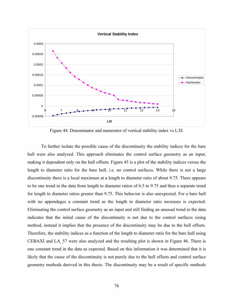
Vertical Stability Index

-0.00005

0

0.00005

0.0001

0.00015

0.0002

0.00025

0.0003

6 7 8 9 10 11 12 13 14

L/D

DenominatorNumerator

Figure 44. Denominator and numerator of vertical stability index vs L/D.

To further isolate the possible cause of the discontinuity the stability indices for the bare

hull were also analyzed. This approach eliminates the control surface geometry as an input,

making it dependent only on the hull offsets. Figure 45 is a plot of the stability indices versus the

length to diameter ratio for the bare hull, i.e. no control surfaces. While there is not a large

discontinuity there is a local maximum at a length to diameter ratio of about 9.75. There appears

to be one trend in the data from length to diameter ratios of 6.5 to 9.75 and then a separate trend

for length to diameter ratios greater than 9.75. This behavior is also unexpected. For a bare hull

with no appendages a constant trend as the length to diameter ratio increases is expected.

Eliminating the control surface geometry as an input and still finding an unusual trend in the data

indicates that the initial cause of the discontinuity is not due to the control surfaces sizing

method, instead it implies that the presence of the discontinuity may be due to the hull offsets.

Therefore, the stability indices as a function of the length to diameter ratio for the bare hull using

CEBAXI and LA_57 were also analyzed and the resulting plot is shown in Figure 46. There is

one constant trend in the data as expected. Based on this information it was determined that it is

likely that the cause of the discontinuity is not purely due to the hull offsets and control surface

geometry methods derived in this thesis. The discontinuity may be a result of specific methods

76

utilized by GEORGE for specific calculations and there may be limitations to those methods that

are unknown for the scope of this thesis.

Figure 45. Stability indices vs. L/D for bare hull.

Figure 46. Stability indices vs L/D for bare hull data using CEBAXI and LA_57.

5.2 CEBAXI and LA_57 Dynamic Stability Model

Four separate design of experiments were performed using the CEBAXI and LA_57

model; one for each stern and forward plane configuration (sail planes with an x-stern, sail

planes with a cruciform stern, bow planes with an x-stern, and bow planes with a cruciform

77

stern). The resulting plots for the DOE and RSM are provided in Appendix D. For each DOE the

Latin-Hypercube algorithm was chosen to ensure sufficient exploration of the entire design space

and the number of runs was set to 200. Four design variables were examined: length to diameter

ratio, diameter, aft body fullness factor, and forward body fullness factor. Table 15 shows the

specified range for each design variable. The horizontal and vertical stability indices, GH and GV,

were the two response variables examined. The data sets created by the DOE were then analyzed

and any outliers were deleted before further analysis was performed. An outlier was determined

as a data set whose values were significantly outside of the apparent trend of the data. The

modified data sets were then used to develop the corresponding RSM. The following sections

detail the results of the four design of experiments that were performed and their resulting

response surfaces.

Table 15. Design variables and high and low boundaries for CEBAXI and LA_57 stability model.

Design Variable Low High L/D 6.5 13

D (ft) 22 32 na 2.5 3.5 nf 2 3

5.2.1 Configuration 1: Sail planes with an X-stern

Figure 47 and Figure 48 are plots of the main effects for the horizontal and vertical

stability indices and demonstrate the sensitivity of the variables to one another. They show that

the length to diameter ratio and diameter design variables have the greatest effect on the both of

the stability indices for this configuration.

78

Figure 47. Gh main effects for CEBAXI and LA_57 configuration 1.

Figure 48. Gv main effects for CEBAXI and LA_57 configuration 1.

Figure 49 shows how the stability indices vary as a function of the length to diameter

ratio. In general, the stability indices increase with increasing length to diameter ratios showing

that long and slender submarines are more stable than short and fat submarines. Stable designs

(indices greater than zero) do not occur until a length to diameter ratio of approximately 8.25. At

79

a length to diameter ratio near 11.5 stability in both the horizontal and vertical planes begins to

plateau at values close to one indicating highly stable submarines.

Figure 49. Stability indices vs L/D for configuration 1.

Figure 50 and Figure 51 are variable influence plots. The variable influence plots show

both the main effects and interaction effects of the design variables. Higher order effects involve

more than two variables and are grouped together into one category. The other category includes

variables with an importance less than 0.5% for both stability indices the length to diameter ratio

has the most influence. Therefore, Figure 50 and Figure 51 show that the length to diameter ratio

has the most influence on both stability indices and the higher order effects are not of great

importance.

80

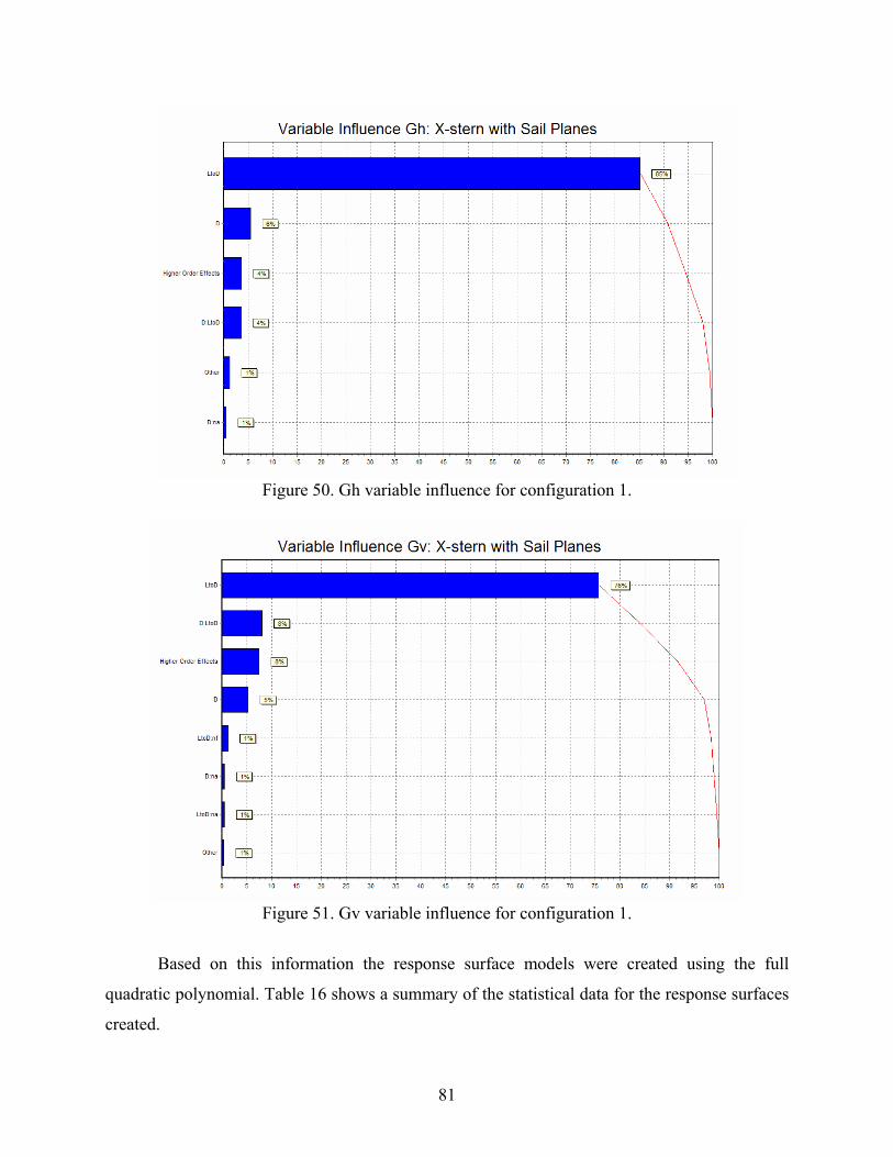
Figure 50. Gh variable influence for configuration 1.

Figure 51. Gv variable influence for configuration 1.

Based on this information the response surface models were created using the full

quadratic polynomial. Table 16 shows a summary of the statistical data for the response surfaces

created.

81

Table 16. Statistical summary of RSM results for configuration 1.

X-stern with Sail Planes Gh Gv

S 0.1089 0.1348Cov (%) 27.34 29.41 R² (%) 95.83 94.71

R²adj (%) 95.51 94.3

5.2.2 Configuration 2: X-stern with bow planes

Figure 52 and Figure 53 show that the length to diameter ratio and aft body fullness

factor have the most influence on the stability indices and that diameter had less of an affect than

in the X-stern configuration with sail planes (configuration 1).

Figure 52. Gh main effects for configuration 2.

82

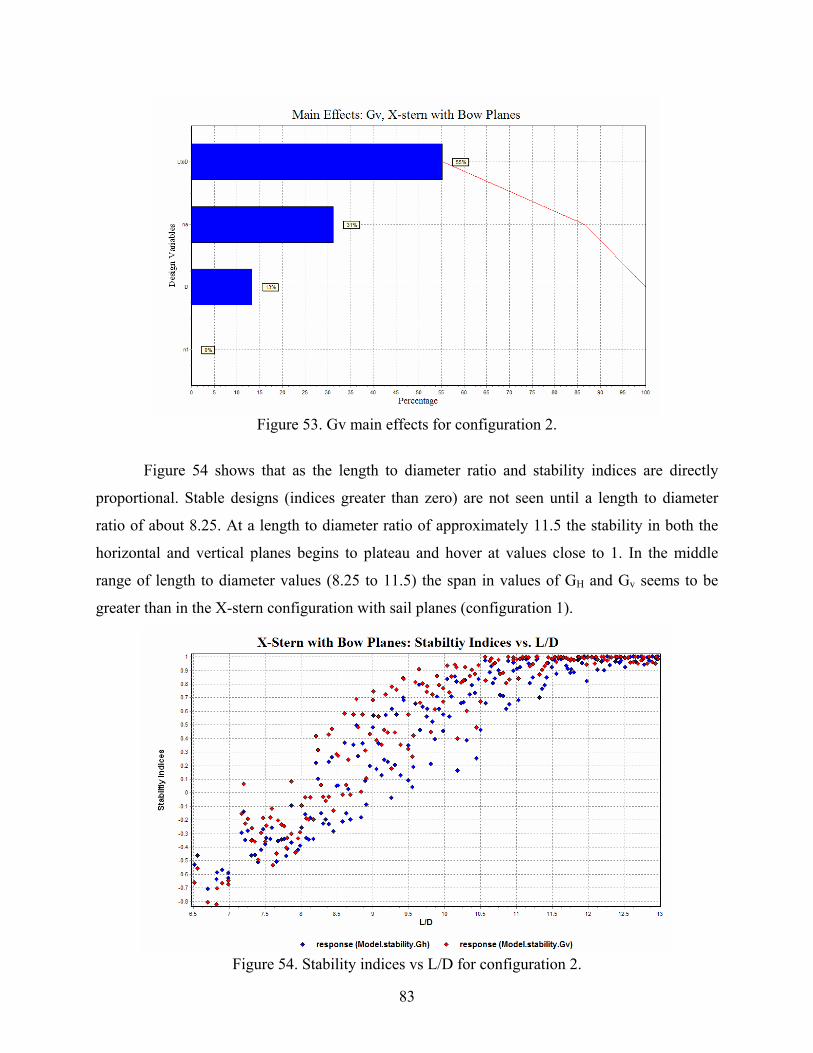
Figure 53. Gv main effects for configuration 2.

Figure 54 shows that as the length to diameter ratio and stability indices are directly

proportional. Stable designs (indices greater than zero) are not seen until a length to diameter

ratio of about 8.25. At a length to diameter ratio of approximately 11.5 the stability in both the

horizontal and vertical planes begins to plateau and hover at values close to 1. In the middle

range of length to diameter values (8.25 to 11.5) the span in values of GH and Gv seems to be

greater than in the X-stern configuration with sail planes (configuration 1).

Figure 54. Stability indices vs L/D for configuration 2.

83

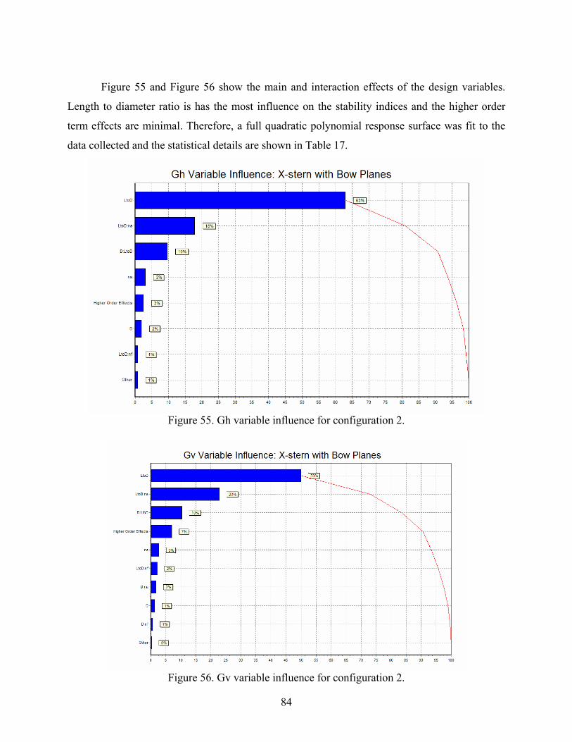
Figure 55 and Figure 56 show the main and interaction effects of the design variables.

Length to diameter ratio is has the most influence on the stability indices and the higher order

term effects are minimal. Therefore, a full quadratic polynomial response surface was fit to the

data collected and the statistical details are shown in Table 17.

Figure 55. Gh variable influence for configuration 2.

Figure 56. Gv variable influence for configuration 2.

84

Table 17. Statistical summary of RSM results for configuration 2.

X-stern with Bow Planes Gh Gv

S 0.1232 0.1199 Cov (%) 29.2 22.78 R² (%) 95.21 95.3

R²adj (%) 94.83 94.92

5.2.3 Configuration 3: Cruciform Stern with Sail Planes

Figure 57 and Figure 58 show that the length to diameter ratio and forward body fullness

factor have the greatest effect on the stability indices.

Figure 57. Gh main effects for configuration 3.

85

Figure 58. Gv main effects for configuration 3.

Figure 59 is a plot of the stability indices versus the length to diameter ratio. As the length to

diameter ratio increases the stability indices increase. Designs with a length to diameter ratio

approximately equal to or greater than 8 have stability in both the horizontal and vertical planes.

For the designs with a length to diameter ratio less than 8 some have stability in the vertical

plane, but none have horizontal plane stability. At a length to diameter ratio of 11.5 and greater

stability in both planes plateaus to values close to one, indicating designs that are highly stable,

but have limited maneuverability.

86

Figure 59. Stability indices vs. L/D for configuration 3.

Figure 60 and Figure 61 display the main and interaction effects for this configuration. The

length to diameter ratio is the dominating effect and the higher order terms have little influence

on the stability indices. Therefore, a full quadratic response surface was created. The statistical

details of the horizontal and vertical stability indices response surfaces are shown in Table 18.

87

Figure 60. Gh variable influence for configuration 3.

Figure 61. Gv variable influence for configuration 3.

88

Table 18. Statistical summary of RSM results for configuration 3.

Cruciform Stern with Sail Planes Gh Gv

S 0.1025 0.0877 Cov (%) 22.25 14.51 R² (%) 95.9 95.65

R²adj (%) 95.57 95.3

5.2.4 Configuration 4: Cruciform Stern with Bow Planes

A summary of the main effects for each stability index is shown in Figure 62 and Figure 63.

The length to diameter ratio has the greatest influence on both the horizontal and vertical

stability indices.

Figure 62. Gh main effects for configuration 4.

89

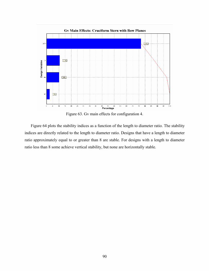
Figure 63. Gv main effects for configuration 4.

Figure 64 plots the stability indices as a function of the length to diameter ratio. The stability

indices are directly related to the length to diameter ratio. Designs that have a length to diameter

ratio approximately equal to or greater than 8 are stable. For designs with a length to diameter

ratio less than 8 some achieve vertical stability, but none are horizontally stable.

90

Figure 64. Stability indices vs L/D for configuration 4.

Figure 65 and Figure 66 show the main and interaction effects for the horizontal and vertical

stability indices respectively. The length to diameter ratio is the dominating variable and the

higher order terms have little effect. Therefore, a full quadratic polynomial was used to create the

horizontal and vertical response surfaces. The statistical details of these response surfaces are

provided in Table 19.

91

Figure 65. Gh variable influence for configuration 4.

Figure 66. Gv variable influence for configuration 4.

92

Table 19. Statistical summary of RSM results for configuration 4.

Cruciform Stern with Bow Planes Gh Gv S 0.086 0.0727

Cov (%) 17.65 11.68 R² (%) 97.27 96.84

R²adj (%) 97.04 96.59

5.2.5 Summary

A design of experiments was performed for each forward plane and stern plane configuration

and based on the data collected corresponding response surfaces were created. For all four

configurations the length to diameter ratio had the greatest impact on the stability indices. For x-

stern configuration stability in both the horizontal and vertical planes was not reached until a

length to diameter ratio of approximately 8.25. For cruciform stern configurations stability was

achieved in both planes at a length to diameter ratios of approximately 8 or greater. Stability for

both planes began to plateau at values close to one for length to diameter ratios of 11.5 and

greater for all configurations. The difference between the values for the horizontal and vertical

stability indices for a given design is greater for designs with a cruciform stern. Therefore, based

on the criteria set in Chapter 2 to guarantee a good tradeoff of stability and maneuverability for

the individual indices (GH should vary from 0.15 to 0.30 and Gv should vary form 0.5 to 0.7) the

data collected shows that a cruciform stern would be the most effective towards meeting this

criteria.

In all configurations, there were fewer designs evaluated at the lowest range of length to

diameter ratios, specifically from length to diameter ratios in the range of 6.5 to 8. This is

because this range had a high number of data sets that were outliers and deleted before analysis

was performed. This concentration of outliers is suspected to be due to two different factors. One

factor is that the CEBAXI program designed to make boundary layer approximation necessary to

run LA_57 is sensitive to the placement of the stern planes on the aft end of the hull. If the stern

planes are placed at a point on the hull where the radius is too large then the program has

difficulty creating the stern velocity profiles. This causes the program to either stop its execution

without producing any data or to produce velocity profiles that may be poor approximations. The

other factor to consider is that the control surface database was created using designs that had a

range of length to diameter ratios from 8 to 13. Designs with a ratio less than 8 were not included

because it was difficult to find these designs. A linear trendline was used to fit the control surface 93

data so that it could be easily extrapolated to included designs with a lower length to diameter

ratio. The fact that the data collected at these lower ratios may indicate that this linear

assumption at low length to diameter ratios is not an appropriate assumption. This would also

explain why there were no designs below a length to diameter ratio of 8 that were stable. It is

known that shorter, fat submarines are inherently more unstable than long, slender submarines.

Therefore, the designs with a smaller length to diameter ratio need larger control surfaces to

increase stability. The assumption of a linear trendline would again not be accurate.

5.3 GEORGE and CEBAXI and LA_57 Comparison

The results obtained from CEBAXI and LA_57 model differed from the results of the

GEORGE model. CEBAXI and LA_57 model did not show significant discontinuities in the data

like those shown in the GEORGE model. CEBAXI and LA_57 model did have difficultly

predicting the stability indices at the upper and lower bounds of the ranges explored but this is

most likely a consequence of the data used to create the control surface database as discussed in

Section 5.2.5. Based on these conclusions it was determined that CEBAXI and LA_57 model

provided the most reasonable data.

94

CHAPTER 6 CONVENTIONAL GUIDED MISSILE SUBMARINE (SSG(X)) DESIGN CASE STUDY

This chapter describes a case study based on the concept exploration of a submarine from

Virginia Tech’s 2006 Senior Design course. Section 1.2 describes the general multi-objective

optimization process used in this course. This chapter describes the SSG(X) required missions

and the OMOE (Overall Measure of Effectiveness) metrics used to assess the design. The

response surfaces created in Chapter 5 are included as part of the OMOE evaluation for the

design. The details of the submarine synthesis model are described and an optimization is set up,

run, and the results discussed.

6.1 SSG(X) Mission Definition and OMOE Development

SSG(X) is a conventional guided missile submarine developed to perform two main

missions:

1. Time sensitive and covert missile and torpedo launch.

2. Covert Intelligence, Surveillance, and Reconnaissance (ISR) operations.

In addition, the SSG(X) should be designed for minimum cost. The lead-ship acquisition cost

should be less than $1B and the follow-ship acquisition cost should be no more than $700M. The

platform must be highly producible to minimize time from concept to delivery. It should also be

flexible enough to support variants. The platform must operate within current logistics support

capabilities and it must consider inter-service and C4/I. The design should focus on survivability

in a high-threat environment and operation in all warfare areas. The platform should be non-

nuclear since the SSG(X) will operate in enemy littoral regions. A typical mission scenario for

each mission is described in Table 20 and Table 21.

Table 20. ISR Mission Scenario [1]. Day Mission scenario

1-15 Depart from CONUS on snorkel to area of hostilities 15-16 Proceed independently to within 10 nautical miles (nm) of enemy mainland 16-20 Conduct ISR 16 Avoid/neutralize enemy submarine attack 17 Conduct mine counter warfare. Launch counter mine AUVs that will detect and neutralize threat. 20-30 Continue ISR 28 Engage enemy patrol craft using Harpoon cruise missile 30 Return to sea base for rearming and refueling

95

Table 21. Missile Mission Scenario [1]. Day Mission scenario

1-15 Depart from home base submerged. Transit at snorkel depth, having batteries charged upon arrival.

15 Launch strike missiles against land target. Launch anti-air defense against an enemy ASW helicopter.

16 Kill incoming cruise missile salvo against CBG in cooperation with DDG. 17 Avoid/neutralize enemy submarine attack 18 Receive re-targeting information and perform cruise missile strike against updated targets. 19-20 Conduct mine counter warfare. Launch counter mine AUVs that will detect and neutralize threat. 15-30 Conduct EM, visual and radio reconnaissance 20 Replenish fuel and stores at sea base 25 Cooperatively, with Aegis unit, detect, engage, and kill incoming cruise missile salvo on CBG unit 26 Engage and destroy enemy surface ships using Harpoon cruise missiles 30 Return to sea base for rearming and refueling

Required Operational Capabilities (ROCs) are identified to perform each mission and

measures of performance (MOPs) are defined to specify those capabilities that will vary in the

designs as a function of the submarine Design Variables (DVs). Each MOP is assigned a

threshold and goal value. ROCs and applicable restraints to all designs are specified in Table 22.

Table 22 - ROC/MOP/DV Summary [1].

ROCs Description Applicable Systems and Technology

MOP Related DV

Goal Threshold

AAW 1.2 Support area anti-air defense

VLS; Sea Sentry; BPS-16 Radar; BPS-15 Radar; BSY-1; BSY-2; SUBTICS

AAW C4I/SPW

SAIL VLS SONARSYS

SAIL=1 VLS=1 SONARSYS=1

SAIL=4 VLS=3 SONARSYS=4

AAW 2 Provide anti-air defense in cooperation with other forces

VLS; Sea Sentry; BPS-16 Radar; BPS-15 Radar; BSY-1; BSY-2; SUBTICS; AN/BRAi-34

AAW C4I/SPW

SAIL VLS SONARSYS

SAIL=1 VLS=1 SONARSYS=1

SAIL=4 VLS=3 SONARSYS=4

AAW 9 Engage airborne threats using surface-to-air armament

VLS; Sea Sentry; BPS-16 Radar; BPS-15 Radar; BSY-1; BSY-2; SUBTICS

AAW C4I/SPW

SAIL VLS SONARSYS

SAIL=1 VLS=1 SONARSYS=1

SAIL=4 VLS=3 SONARSYS=4

AMW 6 Conduct airborne autonomous vehicle (AAV) operations

Sea Sentry; BPS-16 Radar; BPS-15 Radar; BSY-1; BSY-2; SUBTICS

AAW C4I/SPW

SAIL SONARSYS

SAIL=1 SONARSYS=1

SAIL=3 SONARSYS=4

ASU 1 Engage surface threats with anti-surface armaments

Full 6 or 4 21” tubes; Sea Sentry; BPS-16 Radar; BPS-15 Radar; BQQ-10 Sonar; BQQ-5 Sonar; BQQ-6 Sonar; Thales Suite Sonar; BSY-1; BSY-2; SUBTICS

ASuW

TORP SONARSYS SAIL VLS

TORP=1 SONARSYS=1 SAIL=1 VLS =1

TORP=9 SONARSYS=4 SAIL=4 VLS =3

ASU 1.1 Engage surface ships at long range

Full 6 or 4 21” tubes; Sea Sentry; BPS-16

ASuW TORP SONARSYS

TORP=1 SONARSYS=1

TORP=9 SONARSYS=4

96

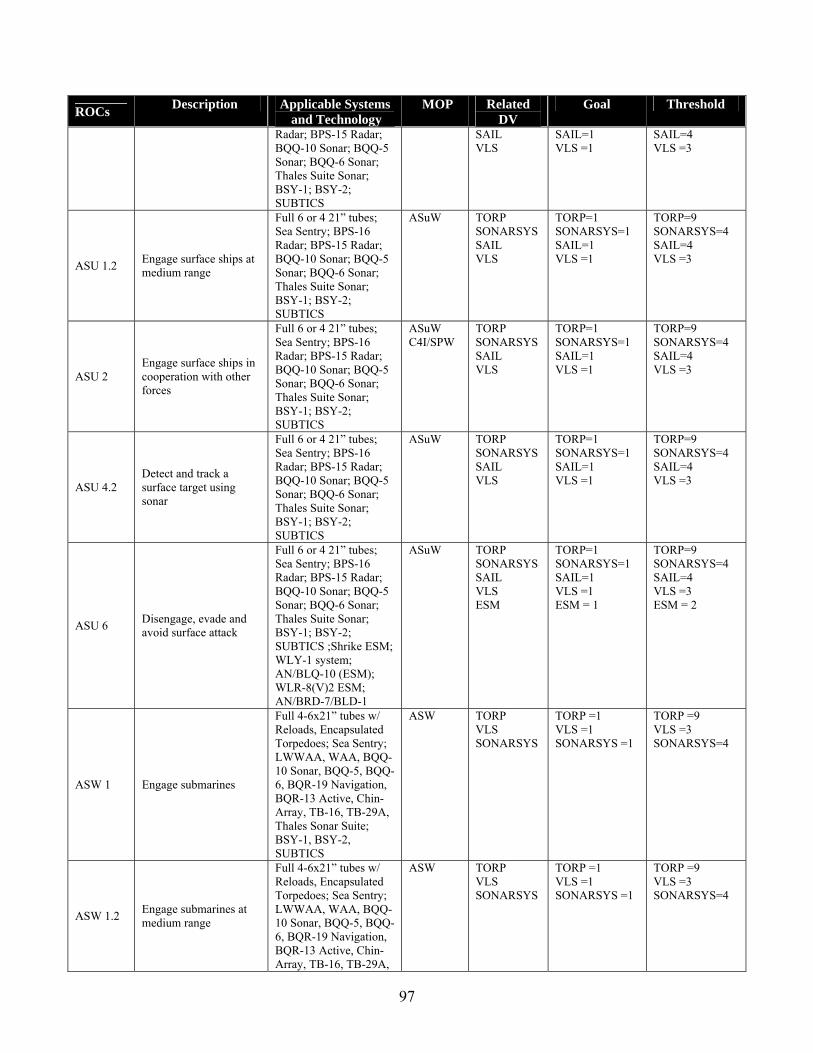
ROCs Description Applicable Systems and Technology

MOP Related DV

Goal Threshold

Radar; BPS-15 Radar; BQQ-10 Sonar; BQQ-5 Sonar; BQQ-6 Sonar; Thales Suite Sonar; BSY-1; BSY-2; SUBTICS

SAIL VLS

SAIL=1 VLS =1

SAIL=4 VLS =3

ASU 1.2 Engage surface ships at medium range

Full 6 or 4 21” tubes; Sea Sentry; BPS-16 Radar; BPS-15 Radar; BQQ-10 Sonar; BQQ-5 Sonar; BQQ-6 Sonar; Thales Suite Sonar; BSY-1; BSY-2; SUBTICS

ASuW TORP SONARSYS SAIL VLS

TORP=1 SONARSYS=1 SAIL=1 VLS =1

TORP=9 SONARSYS=4 SAIL=4 VLS =3

ASU 2 Engage surface ships in cooperation with other forces

Full 6 or 4 21” tubes; Sea Sentry; BPS-16 Radar; BPS-15 Radar; BQQ-10 Sonar; BQQ-5 Sonar; BQQ-6 Sonar; Thales Suite Sonar; BSY-1; BSY-2; SUBTICS

ASuW C4I/SPW

TORP SONARSYS SAIL VLS

TORP=1 SONARSYS=1 SAIL=1 VLS =1

TORP=9 SONARSYS=4 SAIL=4 VLS =3

ASU 4.2 Detect and track a surface target using sonar

Full 6 or 4 21” tubes; Sea Sentry; BPS-16 Radar; BPS-15 Radar; BQQ-10 Sonar; BQQ-5 Sonar; BQQ-6 Sonar; Thales Suite Sonar; BSY-1; BSY-2; SUBTICS

ASuW

TORP SONARSYS SAIL VLS

TORP=1 SONARSYS=1 SAIL=1 VLS =1

TORP=9 SONARSYS=4 SAIL=4 VLS =3

ASU 6 Disengage, evade and avoid surface attack

Full 6 or 4 21” tubes; Sea Sentry; BPS-16 Radar; BPS-15 Radar; BQQ-10 Sonar; BQQ-5 Sonar; BQQ-6 Sonar; Thales Suite Sonar; BSY-1; BSY-2; SUBTICS ;Shrike ESM; WLY-1 system; AN/BLQ-10 (ESM); WLR-8(V)2 ESM; AN/BRD-7/BLD-1

ASuW

TORP SONARSYS SAIL VLS ESM

TORP=1 SONARSYS=1 SAIL=1 VLS =1 ESM = 1

TORP=9 SONARSYS=4 SAIL=4 VLS =3 ESM = 2

ASW 1 Engage submarines

Full 4-6x21” tubes w/ Reloads, Encapsulated Torpedoes; Sea Sentry; LWWAA, WAA, BQQ-10 Sonar, BQQ-5, BQQ-6, BQR-19 Navigation, BQR-13 Active, Chin-Array, TB-16, TB-29A, Thales Sonar Suite; BSY-1, BSY-2, SUBTICS

ASW TORP VLS SONARSYS

TORP =1 VLS =1 SONARSYS =1

TORP =9 VLS =3 SONARSYS=4

ASW 1.2 Engage submarines at medium range

Full 4-6x21” tubes w/ Reloads, Encapsulated Torpedoes; Sea Sentry; LWWAA, WAA, BQQ-10 Sonar, BQQ-5, BQQ-6, BQR-19 Navigation, BQR-13 Active, Chin-Array, TB-16, TB-29A,

ASW TORP VLS SONARSYS

TORP =1 VLS =1 SONARSYS =1

TORP =9 VLS =3 SONARSYS=4

97

ROCs Description Applicable Systems and Technology

MOP Related DV

Goal Threshold

Thales Sonar Suite; BSY-1, BSY-2, SUBTICS

ASW 1.3 Engage submarines at close range

Full 4-6x21” tubes w/ Reloads, Encapsulated Torpedoes; Sea Sentry; SPAT; LWWAA, WAA, BQQ-10 Sonar, BQQ-5, BQQ-6, BQR-19 Navigation, BQR-13 Active, Chin-Array, TB-16, TB-29A, Thales Sonar Suite; BSY-1, BSY-2, SUBTICS

ASW TORP VLS SONARSYS

TORP =1 VLS =1 SONARSYS =1

TORP =9 VLS =3 SONARSYS=4

ASW 2 Engage submarines in cooperation with other forces

Full 4-6x21” tubes w/ Reloads, Encapsulated Torpedoes; Sea Sentry; SPAT; LWWAA, WAA, BQQ-10 Sonar, BQQ-5, BQQ-6, BQR-19 Navigation, BQR-13 Active, Chin-Array, TB-16, TB-29A, Thales Sonar Suite; BSY-1, BSY-2, SUBTICS; AN/BRAi-34

ASW C4I/SPW

TORP VLS SONARSYS

TORP =1 VLS =1 SONARSYS =1

TORP =9 VLS =3 SONARSYS=4

ASW 7 Attack submarines with antisubmarine armament

Full 4-6x21” tubes w/ Reloads, Encapsulated Torpedoes; Sea Sentry; SPAT; LWWAA, WAA, BQQ-10 Sonar, BQQ-5, BQQ-6, BQR-19 Navigation, BQR-13 Active, Chin-Array, TB-16, TB-29A, Thales Sonar Suite; BSY-1, BSY-2, SUBTICS, MK 60 Mine Launcher

ASW MIW

TORP VLS SONARSYS

TORP =1 VLS =1 SONARSYS =1

TORP =9 VLS =3 SONARSYS=4

ASW 7.6 Engage submarines with torpedoes

Full 4-6x21” tubes w/ Reloads, Encapsulated Torpedoes; Sea Sentry; SPAT; LWWAA, WAA, BQQ-10 Sonar, BQQ-5, BQQ-6, BQR-19 Navigation, BQR-13 Active, Chin-Array, TB-16, TB-29A, Thales Sonar Suite; BSY-1, BSY-2, SUBTICS

ASW TORP VLS SONARSYS

TORP =1 VLS =1 SONARSYS =1

TORP =9 VLS =3 SONARSYS=4

ASW 8 Disengage, evade, avoid and deceive submarines

Full 4-6x21” tubes w/ Reloads, Encapsulated Torpedoes; Sea Sentry; SPAT; LWWAA, WAA, BQQ-10 Sonar, BQQ-5, BQQ-6, BQR-19 Navigation, BQR-13 Active, Chin-Array, TB-16, TB-29A, Thales Sonar Suite; BSY-1, BSY-2, SUBTICS; 3”-6.75” Countermeasure

ASW ESM IR Acoustic

TORP VLS SONARSYS PSYStype PROPtype

TORP =1 VLS =1 SONARSYS =1 PSYStype =6 PROPtype =1

TORP =9 VLS =3 SONARSYS =4 PSYStype =4 PROPtype =2

98

ROCs Description Applicable Systems and Technology

MOP Related DV

Goal Threshold

Launcher w/ Reloads;

CCC 3 Provide own unit Command and Control

BSY-1, BSY-2, SUBTICS

C4I/SPW SONARSYS SONARSYS =1 SONARSYS =4

CCC 4 Maintain data link capability

BSY-1, BSY-2, SUBTICS

C4I/SPW SONARSYS SONARSYS =1 SONARSYS =4

CCC 6 Provide communications for own unit

BSY-1, BSY-2, SUBTICS

C4I/SPW SONARSYS SONARSYS =1 SONARSYS =4

CCC 9 Relay communications

BSY-1, BSY-2, SUBTICS; BPS-16 Radar; AN/BRAi-34; EHF/SHF HDR Multiband; IEM; OE-315 HSBCA

C4I/SPW SONARSYS SONARSYS =1 SONARSYS =4

CCC 21 Perform cooperative engagement

BSY-1, BSY-2, SUBTICS; BPS-16 Radar; AN/BRAi-34; EHF/SHF HDR Multiband; IEM; OE-315 HSBCA

C4I/SPW SONARSYS SONARSYS =1 SONARSYS =4

FSO 3 Provide support services to other units

All Designs N/A

FSO 5 Conduct towing/search/salvage rescue operations

All Designs N/A

FSO 6 Conduct SAR operations

All Designs N/A

FSO 7 Provide explosive ordnance disposal services

All Designs N/A

FSO 9 Provide routine health care

All Designs N/A

FSO 10 Provide first aid assistance

All Designs N/A

INT 1 Support/conduct intelligence collection

Sea Sentry; Full 4-6x21” tubes w/ Reloads; BSY-1, BSY-2, SUBTICS; 4-man lock out

C4I/SPW TORP SAIL SONARSYS SPW

TORP =1 SAIL =1 SONARSYS =1 SPW =1

TORP =9 SAIL =4 SONARSYS=4 SPW =2

INT 3 Conduct surveillance and reconnaissance

Sea Sentry; Full 4-6x21” tubes w/ Reloads; BSY-1, BSY-2, SUBTICS; 4-man lock out

C4I/SPW TORP SAIL SONARSYS SPW

TORP =1 SAIL =1 SONARSYS =1 SPW =1

TORP =9 SAIL =4 SONARSYS=4 SPW =2

INT 9

Disseminate surveillance and reconnaissance information

Sea Sentry; Full 4-6x21” tubes w/ Reloads; BSY-1, BSY-2, SUBTICS; 4-man lock out

C4I/SPW TORP SAIL SONARSYS SPW

TORP =1 SAIL =1 SONARSYS =1 SPW =1

TORP =9 SAIL =4 SONARSYS=4 SPW =2

MIW 3 Conduct mine neutralization/ destruction

Full 4-6x21” tubes w/Reloads; BSY-1, BSY-2, SUBTICS;

MIW TORP SONARSYS

TORP =1 SONARSYS =1

TORP =9 SONARSYS=4

MIW 3.1

Deploy AUVs and UUVs for mine detection and neutralization

Full 4-6x21” tubes w/Reloads; Sea Sentry; UUV’s; BSY-1, BSY-2, SUBTICS;

MIW TORP SONARSYS

TORP =1 SONARSYS =1

TORP =9 SONARSYS=4

MIW 4 Conduct mine avoidance

Full 4-6x21” tubes w/Reloads; BSY-1, BSY-2, SUBTICS;

MIW TORP SONARSYS

TORP =1 SONARSYS =1

TORP =9 SONARSYS=4

MIW 6 Conduct magnetic silencing (Ndegaussing, deperming)

Ndegaussing Magnetic Signature

NDEGAUS=1 NDEGAUS =0

MIW 6.7 Maintain magnetic signature limits

Ndegaussing Magnetic Signature

NDEGAUS =1 NDEGAUS =0

99

ROCs Description Applicable Systems and Technology

MOP Related DV

Goal Threshold

MOB 1 Steam to design capacity in most fuel efficient manner

Hull, Propulsion Speed Sprint, End; End Range Snorkel, AIP, Sprint

Hullform, PSYStype, PROPtype

Esnork =4000 nm Eaip =30 days Vs=22 knt Es=2hr

Esnork=3000 nm Eaip=20 days Vs=15 knt Es=1hr

MOB 3 Prevent and control damage

All Designs N/A

MOB 7

Perform seamanship, airmanship and navigation tasks (navigate, anchor, mooring, scuttle, life boat/raft capacity, tow/be-towed)

All Designs N/A

MOB 10 Replenish at sea All Designs N/A

MOB 12 Maintain health and well being of crew

All Designs N/A

MOB 13

Operate and sustain self as a forward deployed unit for an extended period of time during peace and war without shore-based support

All Designs N/A Ts 45days 25days

MOB 16 Operate in day and night environments

All Designs N/A

MOB 17 Operate in heavy weather

Hullform STABI Depth 1000 ft 500 ft

MOB 18

Operate in full compliance of existing US and international pollution control laws and regulations

All Designs N/A

MOB 19 Operate submerged using AIP and batteries

Propulsion, Batteries End AIP PSYStype, BAT, BATC, WFAIP

Ebat =9000kwhr WFaip=200lt

Ebat =2500kwhr WFaip=100lt

MOB 20 Operate and transit on snorkel

Propulsion; Snorkel End Snorkel and Speed

SAIL, PSYStype, WFS

SAIL=1 WFsnork=200lt

SAIL=2 WFsnork=100lt

NCO 3 Provide upkeep and maintenance of own unit

All Designs N/A

SEW 2 Conduct sensor and ECM operations

Shrike ESM; WLY-1; AN/BLQ-10 (ESM); WLR-8(v)2 interceptors; AN/BRD-7/BLD-1

AAW, ASuW, MIW, ASW,

ESM

ESM =1 ESM =2

SEW 5 Conduct coordinated SEW operations with other units

Shrike ESM; WLY-1; AN/BLQ-10 (ESM); WLR-8(v)2 interceptors, AN/BRD-7/BLD-1; EHF/SHF HDR Multi-band; AN/BRAi-34; OE-315 HSBCA

AAW, ASuW, MIW, ASW, C4I/SPW

ESM SAIL

ESM =1 SAIL=1

ESM =2 SAIL=2

STW 3 Support/conduct multiple cruise missile strikes

VLS, BSY-1, BSY-2, SUBTICS

STK VLS, SONARSYS

VLS =1 SONARSYS =1

VLS =3 SONARSYS=4

100

An OMOE hierarchy, shown in Figure 67, is developed based on the defined MOPs,

summarized in Table 23. AHP and pair-wise comparison are used to calculate MOP weights and

Multi-Attribute Value Theory (MAVT) is used to develop individual MOP value functions.

Expert and customer opinion are required to calculate AHP weights using pair-wise comparison

questionnaires. VOPs (Values of Performance) are calculated for each MOP using VOP

functions, usually S-curves. A VOP of 0 corresponds to the MOP threshold value, while a VOP

of 1.0 corresponds to the MOP goal value .The result is the weighted overall effectiveness

function (OMOE) as described in Section 1.2.1 to be used as an objective in the multi-objective

optimization.

Table 23. MOP Table [1]. MOP # MOP Metric Goal Threshold

1 AAW

VLS Option SONARSYS Option SAIL Option ESM Option

VLS =1 SONARSYS =1 SAIL =1 ESM =1

VLS =3 SONARSYS=4 SAIL =4 ESM =2

2 ASW

TORP Option VLS Option SONARSYS Option SAIL Option ESM Option

TORP =1 VLS =1 SONARSYS =1 SAIL =1 ESM =1

TORP =9 VLS =3 SONARSYS=4 SAIL =4 ESM =2

3 ASuW

SONARSYS Option SAIL Option TORP Option ESM Option VLS Option

SONARSYS =1 SAIL =1 TORP =1 ESM =1 VLS =1

SONARSYS=4 SAIL =4 TORP =9 ESM =2 VLS =3

4 C4I/SPW

SONARSYS Option SAIL Option TOR Option SPW Option

SONARSYS =1 SAIL =1 TOR =1 SPW =1

SONARSYS=4 SAIL =4 TOR =9 SPW =2

5 STK SONARSYS Option SAIL Option VLS Option

SONARSYS =1 SAIL =1 VLS =1

SONARSYS=4 SAIL =4 VLS =3

6 MIW SONARSYS Option SAIL Option TORP Option

SONARSYS =1 SAIL =1 TORP =1

SONARSYS=4 SAIL =4 TORP =9

7 Vs (Sprint Speed) Knots 22knts 15knts

8 Es (Sprint Duration) Hr 2hr 1hr

9 Esnork (@ 12 knts) nm 4000nm 3000nm

10 Eaip (AIP Duration @ 5 knts) Days 30days 20days

11 Depth Feet 1000ft 500ft

12 STABI Index 4 1

13 Hull Vulnerability Depth (ft) 1000 500

14 Acoustic Signature PSYStype PROPtype

PSYStype =5 PROPtype =1

PSYStype =3 PROPtype =2

15 IR Signature PROPtype PROPtype =1 PROPtype =2

16 Magnetic Signature DEGAUS Ndegaus =1 Ndegaus =0

101

Figure 67 . OMOE Hierarchy

ISR or Missile Launch

War Fighting Mobility

Susceptibility

AAW ASW

ASuW MIW

CCC INT

STK

Sprint Speed

Sprint Endurance

Depth

Environmental

Structure

Acoustic Signature IR Signature

Magnetic Signature

Endurance Snorkel Speed

Endurance AIP

Endurance Snorkel

Ts (Stores)

Sustainability

Dynamic Stability

6.2 Submarine Synthesis Model [1]

The submarine synthesis model shown in Figure 3 defines and balances designs selected by

the optimizer and assesses their feasibility, effectiveness, risk, and cost. It is developed in

ModelCenter.

The Ship Synthesis Model is organized into the following modules:

• Input Module: Stores the design variable values and other design parameters which

are provided as input to the other modules.

• Combat Module: Sums payload characteristics (weights, vertical centers of gravity

(VCGs), arrangeable areas, and electric power consumption) using the combat system

alternatives selected and an Excel file containing data for each system. The weights,

arrangeable areas, and electric power consumption are simple summations; vertical

centers of gravity are calculated using moments of weights. The combat module

102

outputs weights summarized by SWBS groups as well as a total, arrangeable area,

power consumption, and the required payload outboard volume.

• Propulsion Module: Calculates propulsion and generator system characteristics

(weights and stowage volumes) using the propulsion “subsystems” (propulsion

system, propulsor type, battery type) alternatives and capacities (battery capacity, fuel

weight (AIP), fuel weight (snorkel)) and an Excel file containing data (stowage and

machinery room volumes, fuel consumption rates, and transmission efficiency). It

also uses the battery type to determine battery and performance characteristics. The

Propulsion Module outputs the battery power, weight and volume of the basic

propulsion machinery, batteries and fuels, the volume of the prop, specific fuel

consumption (SFC), power provided by AIP and snorkeling, AIP diesel fuel energy

capacity, overall propulsive coefficient (PC), and transmission efficiency.

• Hull Module: Calculates hull characteristics (volumes and lengths of the three hull

parts and the total bare hull surface area) using hull input quantities (diameter, beam-

to-diameter ratio, length-to-diameter ratio and forward and aft fullness exponents).

These quantities are used to find a shape defined using an MIT model (see Figure 24)

which is composed of an ellipsoidal forebody, parallel midbody, parabolic aftbody,

and transverse midbody; this hull form is a modified form of the hydrodynamically

optimized teardrop hullform which adds parallel midbody (length) and transverse

midbody (beam) to provide more arrangeable area. The Hull Module calculates

lengths and offsets based on this model and integrates over the lengths to determine

the volumes of each part. The module outputs the width of the transverse insertion,

the bare hull surface area, the envelope volume, the length of each part of the hull, the

beam, and the length overall.

• Tankage Module: Calculates the tankage volumes and liquid weights and crew

manning numbers. The diesel fuel is split between clean (17%) and compensated

(83%) tanks. Compensated tanks external to the pressure hull use ballast water to

replace diesel fuel as it is used; this allows easier management of ballast and an

overall more efficient design. Soft tanks ballast open to the sea and have a lower

weight. The tankage weights (including AIP liquids) are based on the specific

volumes for the tankage contents. The Tankage Module calculates manning numbers

103

using a parameterized model based on the ship size, power consumption, and

manning and automation factor; these are calculated in the Tankage Module as this is

a convenient place (the Hull Module is the first module to use these numbers).

Additional (habitability) tankage volumes and weights are calculated using the crew

numbers. The tankage module outputs the total inboard tankage volume and the

outboard compensated tankage volume, enlisted and total crew numbers, and the

weights for lube oil, fresh water, sewage, and clean and compensated fuel.

• Space Module: Calculates available and required arrangeable areas and hull volumes

(including free flood and free flood min/max) using the stores and provisions

duration, average deck height, crew numbers (enlisted, officers and total), the

pressure hull arrangeable area margin, and the required area for payload (CCC and

ordnance delivery system). The arrangeable area is calculated using parametric

models; arrangeable area and average deck height are used to calculate the

arrangeable volume; the hull volumes are based on their definitions and previously

calculated volumes. The Space Module outputs various volumes (pressure hull,

outboard displacement, everbuoyant, main ballast tank, submerged displaced, free

flood (including min/max) and auxiliary space; it also outputs the total required and

total available arrangeable area.

• Electric Module: Calculates (with applicable margins) the maximum electric power

load and the 24-hour average load. It inputs the margins (electric functional margin

factor, electric design margin factor and average electric power margin factor),

payload weight, volumes of the pressure hull, machinery box and auxiliary box, the

power provided while snorkeling, overall length and diameter, the required power for

the payload, the total crew number and whether or not there is a degaussing system. It

then calculates the power required using a parameterized model which uses the hull

dimensions, the ship service power based on the total crew number and the total load.

• Resistance Module: Calculates sustained speed, ranges and endurances (sustained,

snorkel and AIP), and the total mission length. The Resistance Module calculates

resistance over a range of speeds using frictional resistance (from the bare hull

surface area) form factor and a correlation allowance. The endurances are based on

battery and fuel capacities and usage rates, the Propulsion Margin Factor (PMF),

104

Overall Propulsive Coefficient (PC), and the transmission efficiency (η). The mission

length is based on the endurances that are calculated.

• Weight Module: Calculates total weights and VCGs for SWBS groups, overall VCG,

stability (GB and GM), and minimum and maximum values for lead ballast. It

calculates SWBS subgroups (systems, subsystems, shafting, cabling, etc.) weights

and VCGs based on inputs. The group weights are found by summing the individual

components and VCGs are calculated using weight moments. The hull geometry

determines the center of buoyancy which is used with the overall VCG to calculate

GB (the submerged stability condition). The surface stability condition (GM) is

calculated using stability formula which considers the waterplane contribution to the

stability. This module also calculates lead weight as difference between NSC weight

and everbuoyant displacement. The feasibility module assesses the feasibility of this

weight to satisfy minimum design and stability lead requirements.

Weight Estimation Volume Estimation

Group 1 (Hull)Group 2 (Propulsion Machinery)Group 3 (Electrical)Group 4 (Electronics)Group 5 (Auxiliary Equipment)Group 6 (Outfit & Furnishings)Group 7 (Weapons)

Condition A-1

ΣGroup 1..7

A-1 + Lead Ballast

Condition A

A + Variable Load

a. Mobilityb. Weaponsc. Command and Controld. Auxiliariese. Habitabilityf. Storerooms

function (a..f)

Pressure Hull Volume (Vph)

factor * Vph

Outboard Volume (Vob)

Vph + Vob

Normal Surface Condition Everbuoyant Volume (Veb)

Balance

Envelope Volume (Venv)

Main Ballast Tank Volume (Vmbt) = factor *Veb

Submerged Volume (Vsub) = Veb + Vmbt

Freeflood Volume (Vff) = factor * Veb

Figure 68: Submarine balance work flow diagram [1].

105

• Feasibility Module: Calculates ratios comparing the actual values of snorkel

endurance range, AIP endurance duration, sustained speed, spring duration,

submerged GB, surfaced GM, weight of lead, free flood, arrangeable area, and the

stores and provisions duration to applicable minimums and/or maximums. Each ratio

must be positive for a feasible design. It also checks if the values of the horizontal

and vertical stability indices fall within the defined stability/maneuverability range.

Each of these ratios and values are output to the MOGO Module to determine if the

design is feasible.

• OMOE Module: Calculates a Value of Performance (VOP) for each Measure of

Performance (MOP) using the actual values calculated and an Overall Measure of

Effectiveness (OMOE). Each VOP is calculated based on weights provided by a

previously-completed pair-wise comparison process. The OMOE (the only output) is

calculated using each VOP added together using weights provided by the pair-wise

comparison. The calculation of the OMOE is further described in Section 1.2.1.

• Cost Module: Calculates the basic cost of construction (CBCC), labor costs for each

SWBS group using complexity factors and SWBS groups weights, material costs

using SWBS groups weights, direct and indirect (using overhead) costs, and the basic

cost of construction using the direct and indirect cost and a profit margin. The

calculation of cost is further described in Section 1.2.2.

• Risk Module: Calculates an Overall Measure of Risk. The OMOR is found by first

calculating a performance, cost, and schedule risk for each system (DVs) based on

risk factors previously determined. The OMOR is a weighted summation of each total

risk for each risk type. The calculation of risk is further described in Section 1.2.3.

• MOGO Module: The Multi-Objective Genetic Optimizer maximizes the OMOE

while complying with the constraints produced by the ratios found in the Feasibility

Module and minimizing the CBCC and OMOR.

106

6.3 Implementation and Integration of Dynamic Stability Models in the

Submarine Synthesis Model in ModelCenter

The response surface models created in Chapter 5 are implemented into the OMOE and

feasibility modules of the submarine synthesis model. The values of the horizontal and vertical

stability indices are calculated in the OMOE module using the created response surfaces. These

values are input into the feasibility module and assessed to determine if they fall in the ranges set

in chapter 2 to ensure a tradeoff in stability and maneuverability (GH should vary between 0.15

and 0.30, GV should vary between 0.5 and 0.7). If the designs do not fall within these ranges then

the design is infeasible.

The stability indices are also implemented in the OMOE module. As shown in Table 23 the

stability indices are defined as a MOP (MOP 12). A VOP function is determined for each index

and is shown in Figure 69 and Figure 70. The VOPs created for the stability indices do not

follow the traditional s-curve used by other VOPs. This is because the ranges defined for the

indices were developed to ensure a tradeoff between stability and maneuverability. Therefore, it

was determined that the midpoint of each range would be the most desirable tradeoff and would

correspond to a VOP of 1, this is the goal value. The threshold values are the upper and lower

bounds of the two ranges. They represent the minimum and maximum tolerable values for the

indices. An overall VOP is calculated as a function of the two stability indices VOPs. For each

index a VOP is determined based on the VOP functions in Figure 69 and Figure 70. Each VOP

contributes to 50% of the overall stability VOP. This overall VOP is used in the OMOE

calculation for each design.

107

Gh

Horizontal Stability Index VOP

0

0.1

0.2

0.3

0.4

0.5

0.6

0.7

0.8

0.9

1

0.15 0.16 0.17 0.18 0.19 0.2 0.21 0.22 0.23 0.24 0.25 0.26 0.27 0.28 0.29 0.3

VOP

Figure 69. VOP for Gh.

Vertical Stability Index VOP

0

0.1

0.2

0.3

0.4

0.5

0.6

0.7

0.8

0.9

1

0.5 0.52 0.54 0.56 0.58 0.6 0.62 0.64 0.66 0.68 0.7

Gv

VO

P

Figure 70. VOP for Gv.

108

6.4 Optimization

The design space is defined by twenty design variables listed in Table 24. The optimizer

chooses values for each variable in the allowable range and the submarine synthesis model uses

these values to balance the design, checks for feasibility, and calculate the measures of

effectiveness, risk, and cost. The optimization utilizes the Darwin optimizer defined in Section

4.1.5 and the optimization is performed as outlined in Section 1.2.4.

Table 24. SSG(X) Design Variables (DVs) DV # DV Name Description Design Space

1 D Diameter 24-34ft 2 LtoD Length to Depth Ratio 7-10 3 BtoD Beam to Depth Ratio 1-1.2 4 na Fullness factor aft 2.5-4 5 nf Fullness factor forward 2.0-3.5 6 Depth Diving Depth 500-1010ft

7 PSYS Propulsion system alternative

Option 1) CCD, CAT 3512 V12 x2 Engines Option 2) CCD, CAT 3516 V16 x2 Engines Option 3) CCD, 2xCAT3516V16 + 2xCAT3512V12 Option 4) CCD, 2xCAT 3608 IL8 Option 5) OCD/AIP, 2xCAT 3512 V12 + 2x250KW PEM Option 6) OCD/AIP, 2xCAT 3512 V12 + 2x500KW PEM Option 7) OCD/AIP, 2xCAT 3516 V16 + 2x250KW PEM Option 8) OCD/AIP, 2xCAT 3516 V16 + 2x500KW PEM Option 9) OCD/AIP, 2x CAT 3608 IL8 + 2x250KW PEM

8 PROPtype Propulsion Prop Type Option 1) RDP, Rim Driven Prop Option 2) Shrouded

9 BATtype Battery system type alternative

Option 1) Nickel Cadmium Option 2) Lead Acid Option 3) Zebra

10 Ebat Battery Capacity 5000-12000 kwhr 11 Wfsnork Weight Fuel Snorkel 50-150lton 12 Wfaip Weight Fuel AIP 300-900lton 13 Ndegaus Degaussing 0=none; 1=degaussing 14 Cman Manpower Reduction 0.5-1.0

15 TORP Torpedo system alternative

Option 1: Reconfigurable torpedo room, 6x21” tubes, 24 reloads Option 2: Reconfigurable torpedo room, 6x21” tubes, 18 reloads Option 3: Reconfigurable torpedo room, 6x21” tubes, 12 reloads Option 4: Reconfigurable torpedo room, 4x21” tubes, 16 reloads Option 5: Reconfigurable torpedo room, 4x21” tubes, 12 reloads Option 6: Reconfigurable torpedo room, 4x21” tubes, 8 reloads Option 7: No torpedo room, 24 external encapsulated Option 8: No torpedo room, 18 external encapsulated Option 9: No torpedo room, 12 external encapsulated

16 VLS Vertical Launching System Alternatives

Option 1: 24 Cell VLS Option 2: 18 Cell VLS Option 3: 12 Cell VLS

109

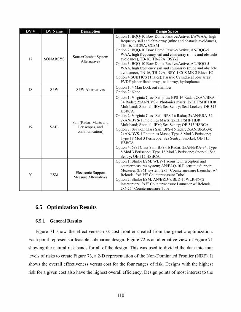
DV # DV Name Description Design Space

17 SONARSYS Sonar/Combat System Alternatives

Option 1: BQQ-10 Bow Dome Passive/Active, LWWAA, high frequency sail and chin-array (mine and obstacle avoidance), TB-16, TB-29A; CCSM

Option 2: BQQ-10 Bow Dome Passive/Active, AN/BQG-5 WAA, high frequency sail and chin-array (mine and obstacle avoidance), TB-16, TB-29A; BSY-2

Option 3: BQQ-10 Bow Dome Passive/Active, AN/BQG-5 WAA, high frequency sail and chin-array (mine and obstacle avoidance), TB-16, TB-29A; BSY-1 CCS MK 2 Block 1C

Option 4:SUBTICS (Thales): Passive Cylindrical bow array, PVDF planar flank arrays, sail array, hydrophones

18 SPW SPW Alternatives Option 1: 4 Man Lock out chamber Option 2: None

19 SAIL Sail (Radar, Masts and

Periscopes, and communication)

Option 1: Virginia Class Sail plus: BPS-16 Radar; 2xAN/BRA-34 Radar; 2xAN/BVS-1 Photonics masts; 2xEHF/SHF HDR Multiband; Snorkel; IEM; Sea Sentry; Seal Locker; OE-315 HSBCA

Option 2: Virginia Class Sail: BPS-16 Radar; 2xAN/BRA-34; 2xAN/BVS-1 Photonics Masts; 2xEHF/SHF HDR Multiband; Snorkel; IEM; Sea Sentry; OE-315 HSBCA

Option 3: Seawolf Class Sail: BPS-16 radar; 2xAN/BRA-34; 2xAN/BVS-1 Photonics Masts; Type 8 Mod 3 Periscope; Type 18 Mod 3 Periscope; Sea Sentry; Snorkel; OE-315 HSBCA

Option 4: 688I Class Sail: BPS-16 Radar; 2xAN/BRA-34; Type 8 Mod 3 Periscope; Type 18 Mod 3 Periscope; Snorkel; Sea Sentry; OE-315 HSBCA

20 ESM Electronic Support Measure Alternatives

Option 1: Shrike ESM; WLY-1 acoustic interception and countermeasures system; AN/BLQ-10 Electronic Support Measures (ESM) system; 2x3” Countermeasure Launcher w/ Reloads, 2x6.75” Countermeasure Tube

Option 2: Shrike ESM; AN/BRD-7/BLD-1; WLR-8(v)2 interceptors; 2x3” Countermeasure Launcher w/ Reloads, 2x6.75” Countermeasure Tube

6.5 Optimization Results

6.5.1 General Results

Figure 71 show the effectiveness-risk-cost frontier created from the genetic optimization.

Each point represents a feasible submarine design. Figure 72 is an alternative view of Figure 71

showing the natural risk bands for all of the design. This was used to divided the data into four

levels of risks to create Figure 73, a 2-D representation of the Non-Dominated Frontier (NDF). It

shows the overall effectiveness versus cost for the four ranges of risk. Designs with the highest

risk for a given cost also have the highest overall efficiency. Design points of most interest to the

110

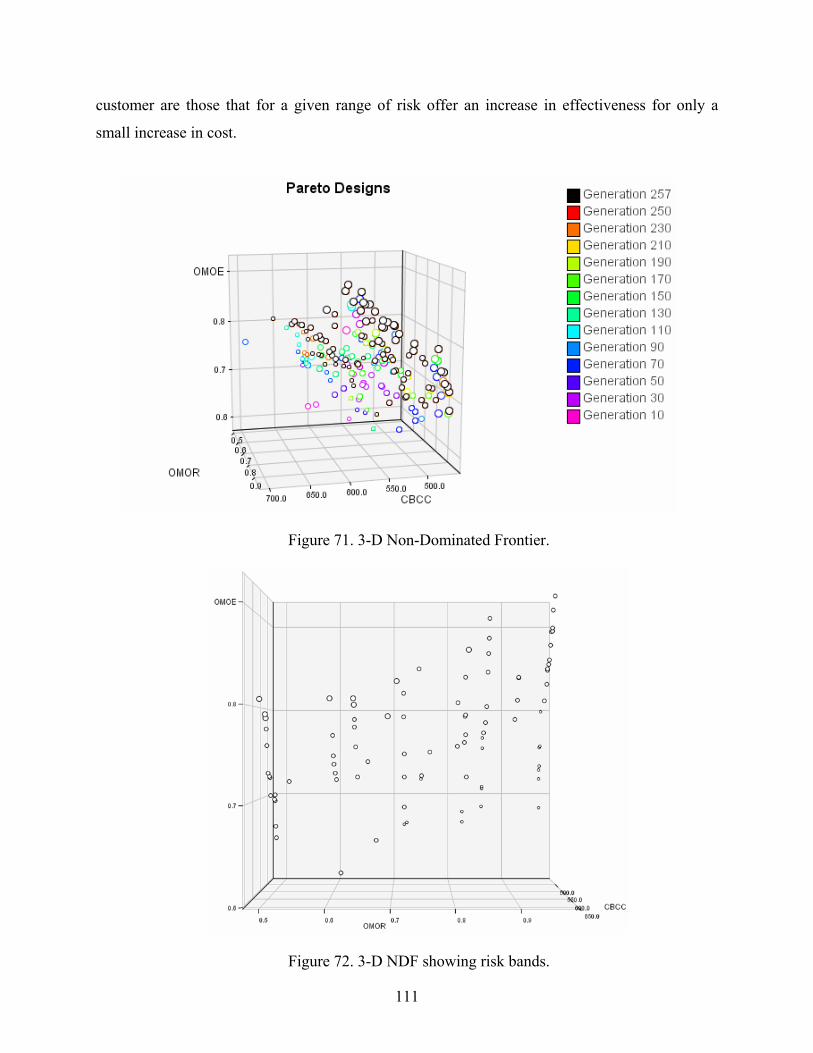
customer are those that for a given range of risk offer an increase in effectiveness for only a

small increase in cost.

Figure 71. 3-D Non-Dominated Frontier.

Figure 72. 3-D NDF showing risk bands.

111

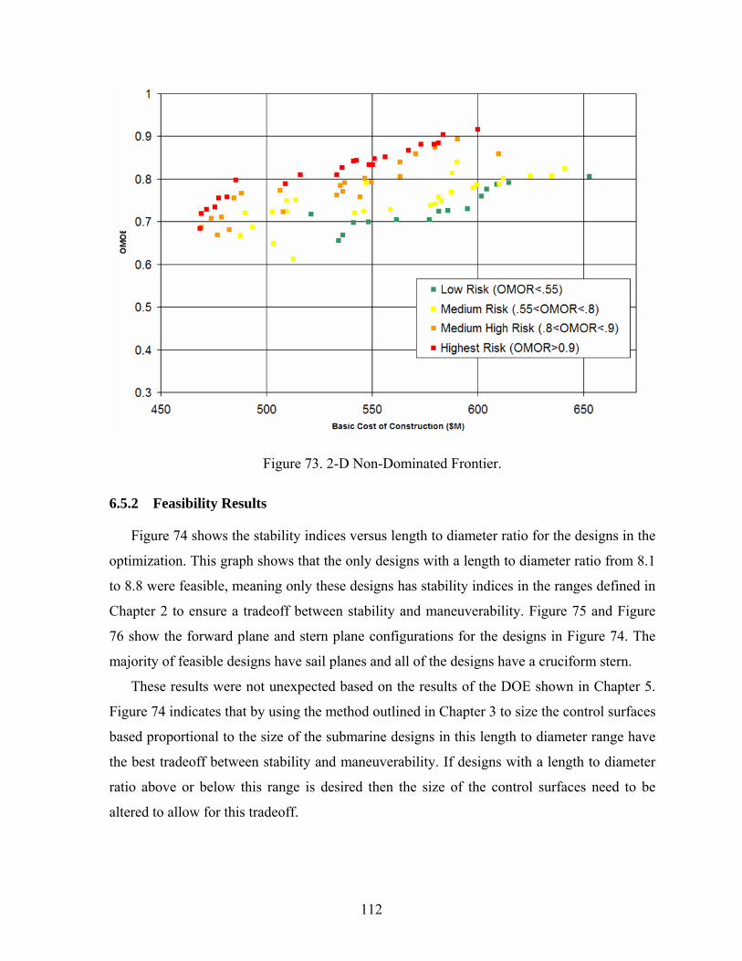
Figure 73. 2-D Non-Dominated Frontier.

6.5.2 Feasibility Results

Figure 74 shows the stability indices versus length to diameter ratio for the designs in the

optimization. This graph shows that the only designs with a length to diameter ratio from 8.1

to 8.8 were feasible, meaning only these designs has stability indices in the ranges defined in

Chapter 2 to ensure a tradeoff between stability and maneuverability. Figure 75 and Figure

76 show the forward plane and stern plane configurations for the designs in Figure 74. The

majority of feasible designs have sail planes and all of the designs have a cruciform stern.

These results were not unexpected based on the results of the DOE shown in Chapter 5.

Figure 74 indicates that by using the method outlined in Chapter 3 to size the control surfaces

based proportional to the size of the submarine designs in this length to diameter range have

the best tradeoff between stability and maneuverability. If designs with a length to diameter

ratio above or below this range is desired then the size of the control surfaces need to be

altered to allow for this tradeoff.

112

Figure 74. Optimization Results: Stability Indices vs. L/D

Figure 75. Optimization Results: Forward plane configuration.

113

Figure 76. Optimization Results: Stern plane configuration.

114

CHAPTER 7 CONCLUSIONS

7.1 Dynamic Stability Model and Case Study Optimization Conclusions

Two tools, GEORGE and CEBAXI and LA_57, were used to analyze horizontal and vertical

plane stability for a submarine during early stage design. Each tool required the hull offsets and

geometry of the control surfaces as input for analysis. The hull offsets were generated based on

an idealized teardrop shape and a control surfaces database was created based on past US Navy

submarine designs to determine sizing trends. These methods were implemented as FORTRAN

programs and integrated with the stability tools in ModelCenter to assess stability. The two tools

were compared and it was determined that GEORGE and CEBAXI and LA_57gave more

reliable results. A design of experiments was performed using GEORGE and CEBAXI and

LA_57 to determine the level of importance of each design variable on the stability indices.

From the data collected response surface models were generated for each configuration analyzed;

sail planes with a cruciform stern, sail planes with an x-stern, bow planes with a cruciform stern,

and bow planes with an x-stern. These response surfaces were implemented as part of the OMOE

in the submarine synthesis model used in the concept exploration phase of the TSSE design

philosophy used at Virginia Tech.

A case study using the SSG(X) design for the Virginia Tech senior design course was

performed using the developed response surfaces and OMOE metrics. The results show that to

achieve the tradeoff of stability and maneuverability specified in Chapter 2 a length to diameter

ratio of approximately 8 to 9 is needed. In addition, a cruciform stern with sail planes was the

best configuration. This process has been integrated into the Senior Design course at Virginia

Tech and has proven to be successful in assessing dynamic stability and control in early stage

design. Figure 77 is a Rhino model of the optimized SSG(X). The dimensions, control surface

configuration, and control surface geometry are all characteristics determined using the process

defined in this thesis.

115

Figure 77. SSG(X) Rhino drawing [1].

7.2 Suggestions for Future Work

The developed process and generated response surfaces have proven to be a good tool to

provide a baseline indication of dynamic stability and control early in the design process. This

section outlines some modifications that can be made to the current process to increase its

robustness and applicability.

As seen in Figure 49, Figure 54, Figure 59, and Figure 64 all designs analyzed during the

design of experiments with a length to diameter ratio less than approximately 8 were unstable in

both the horizontal and vertical plane. This may be a result of the designs used to create the

control surface database. The designs used for the database had length to diameter ratios that

varied from 8 to 13. No data was collected below a length to diameter ratio of 8. Therefore, the

assumption of a linear trendline to model the control surface parameter may not be accurate at

lower length to diameter ratios. A possibility for future study would be to use a quadratic fit to

the data in the control surface database that would increase the size of the control surfaces at

lower length to diameter ratios and see how it affects stability in that length to diameter range.

In addition, the data used to develop the control surface database only included designs with

a cruciform stern configuration. Therefore the only difference between a cruciform stern and x-

stern configuration was the value of the angle Φ as shown in Figure 11; both configurations had

the same dimensions for the control surfaces. One of the advantages of an x-stern is the ability of

the stern planes to have a larger span; therefore, varying the size of the control surfaces based on

the stern configuration would be a possible improvement to the current method. In addition, to

these modifications the presence of the discontinuity that appears in the GEORGE data will

continue to be investigated.

116

117

REFERENCES [1] Alemayehi, D, Boyle, R. Eaton, E, Lynch, T., Stepanchick, J, Yon, R., (2006) “SSG(X)

Guided Missile Design Report.” Virginia Tech Senior Design, Blacksburg, VA. [2] Arentzen, E.S. Capt., Mandel, P. (1960) “Naval Architectural Aspects of Submarine

Design”, SNAME Transactions, Vol. 68, pg 622-692. [3] Brown, A.J., Thomas, M. (1998), "Reengineering the Naval Ship Concept Design

Process", From Research to Reality in Ship Systems Engineering Symposium, ASNE, September, 1998.

[4] Brown, A.J., Salcedo, J. (2002), "Multiple-Objective Optimization In Naval Ship

Design", Naval Engineers Journal, Vol. 115, No. 4. [5] Burcher, R., Rydill, L. (1994), Concepts in Submarine Design. Great Britain: University

Press, Cambridge. [6] Cann, G., Sullivan, P., Brooks, R., Reed, J. (1994), MIT Introduction to Submarine

Design course packet, Cambridge, MA. [7] Chang, M., Moran, T., Junghans, K., Lewis, J., Haussling, H., McCreight, K., Kim, Y.,

(2001) “The Theoretical Prediction of Forces and Moments Acting on an Appended Body of Revolution Performing Arbitrary Maneuvers,” Report No. NSWCCD-50-TR-2001/055, July 2001.

[8] Demko, D., (2006), “Tools for Multi-Objective and Multi-Disciplinary Optimization in

Naval Ship Design.” Blacksburg, VA [9] Fossen, T., (2002). Marine Control Systems. Marine Cybernetics AS, Trondheim,

Norway. [10] GEORGE User Manual, Hydromechanics Division, NCSL Panama City, FL [11] Hover, F., Triantafyllou, M. “Maneuvering and Control of Marine Vehicles.” MIT Open

Courseware, Department of Ocean Engineering, Cambridge, MA. [12] Jones, D., Clarke, D., Brayshaw, I., Barillon, J., Anderson, B., (2002) “The Calculation of

Hydrodynamic Coefficients for Underwater Vehicles,” DSTO Platforms Sciences Laboratory, Australia.

[13] Lewis, E. Ed. (1989). Principals of Naval Architecture, Volume III. SNAME Jersey City,

NJ. [14] ModelCenter Software (2004) Help Files, Phoenix Integration, Blacksburg, VA

118

[15] “US Sea Systems: Data Store-CAD models.” Feb. 2006.www.combatindex.com.

119

APPENDICES

Appendix A - Control Surface Database Designs

(www.combatindex.com)

Figure A1. Top view of Benjamin Franklin class submarine.

Figure A2. Side view of Benjamin Franklin class submarine.

Figure A3. Top view of George Washington class submarine.

Figure A4. Side view of George Washington class submarine.

120

Figure A5. Top view of Ohio class submarine.

Figure A6. Side view of Ohio class submarine.

Figure A7. Top View of Lafayette class submarine.

Figure A8. Side view of Lafayette class submarine.

Figure A9. Top view of Permit class submarine.

121

Figure A10. Side view of Permit class submarine.

Figure A11. Top view of Seawolf class submarine.

Figure A12. Side view of Seawolf class submarine.

Figure A13. Top view of Skipjack class submarine.

122

Figure A14. Side view of Skipjackt class submarine.

Figure A15. Top view of Sturgeon class submarine.

Figure A16. Side view of Sturgeon class submarine.

Figure A17. Top view of Virginia class submarine.

123

Figure A18. Side view of Virginia class submarine.

124

Appendix B – Control Surface Database Plots

Control Surface Parameters vs. Length to Diameter Ratio

Forward Planes: Control Surface Parameter vs. L/D

y = 6.1809x + 11.401

0

20

40

60

80

100

120

6 7 8 9 10 11 12 13 14

L/D

m

Figure B1. Control surface parameter vs. L/D for forward planes.

Horizontal Stern Planes: Control Surface Parameter vs. L/D

y = 5.0462x + 3.1934

0

10

20

30

40

50

60

70

80

90

6 7 8 9 10 11 12 13 14

L/D

m

Figure B2. Control surface parameter vs. L/D for Horizontal Stern Planes.

125

Upper Vertical Stern Plane: Control Surface Parameter vs. L/D

y = 1.4973x + 32.672

0

10

20

30

40

50

60

70

80

6 7 8 9 10 11 12 13 14

L/B

m

Figure B3. Control surface parameter vs. L/D for upper vertical stern planes.

126

Lower Vertical Stern Plane: Control Surface Parameter vs. L/D

y = 2.2979x + 33.315

0

10

20

30

40

50

60

70

80

6 7 8 9 10 11 12 13 14

L/D

m

Figure B4. Control surface parameter vs. L/D for the lower vertical stern plane.

Sail: Control Surface Parameter vs. L/D

y = 0.8198x + 6.182

0

2

4

6

8

10

12

14

16

18

20

6 7 8 9 10 11 12 13 14

L/D

m

Figure B5. Control surface parameter vs. L/D ratio for the sail.

127

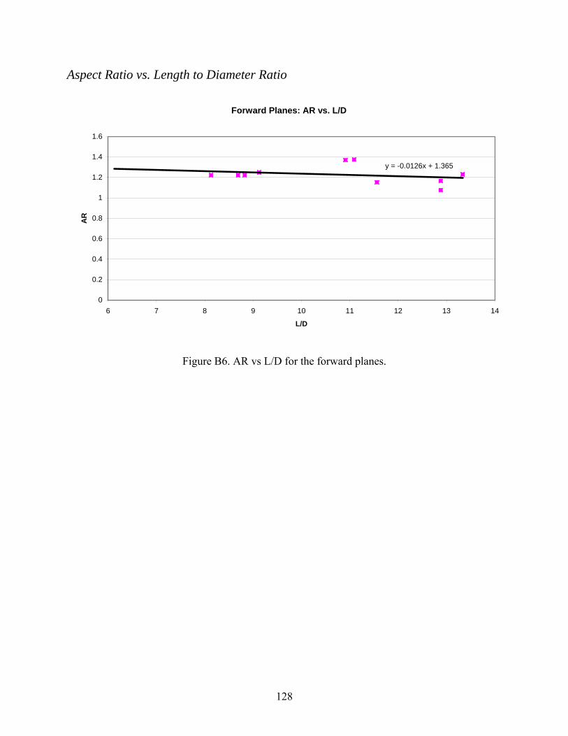
Aspect Ratio vs. Length to Diameter Ratio

Forward Planes: AR vs. L/D

y = -0.0126x + 1.365

0

0.2

0.4

0.6

0.8

1

1.2

1.4

1.6

6 7 8 9 10 11 12 13 14

L/D

AR

Figure B6. AR vs L/D for the forward planes.

128

Horizontal Stern Planes: AR vs. L/D

y = 0.0368x + 1.0452

0

0.2

0.4

0.6

0.8

1

1.2

1.4

1.6

1.8

2

6 7 8 9 10 11 12 13

L/D

AR

14

Figure B7. AR vs L/D for horizontal stern planes.

Upper Vertical Stern Plane: AR vs. L/D

y = 0.0473x + 0.8673

0

0.2

0.4

0.6

0.8

1

1.2

1.4

1.6

1.8

2

6 7 8 9 10 11 12 13 14

L/D

AR

Figure B8. AR vs. L/D for upper vertical stern plane.

129

Lower Vertical Stern Plane: AR vs L/D

y = 0.0405x + 0.7255

0

0.2

0.4

0.6

0.8

1

1.2

1.4

6 7 8 9 10 11 12 13 14

L/D

AR

Figure B9. AR vs. L/D for lower vertical stern plane.

Sail: AR vs. L/D

y = -0.0041x + 0.6825

0

0.1

0.2

0.3

0.4

0.5

0.6

0.7

0.8

0.9

1

6 7 8 9 10 11 12 13 1

L/D

AR

4

Figure B10. AR vs. L/D for the sail.

130

Non-Dimensional Delta Chord vs. Length to Diameter Ratio

Forward Planes: Delta CNon-Dimensional Delta Chord vs. L/D

y = -0.005x + 0.0798

0

0.01

0.02

0.03

0.04

0.05

0.06

6 7 8 9 10 11 12 13 14

L/D

Figure B11. Non-dimensional delta chord vs. L/D for forward planes.

Horizontal Stern Planes: Delta CNon-Dimensional Delta Chord vs. L/D

y = -0.0009x + 0.0301

0

0.005

0.01

0.015

0.02

0.025

0.03

0.035

6 7 8 9 10 11 12 13 1

L/D

4

Figure B12. Non-dimensional delta chord vs. L/D for horizontal stern planes

131

Upper Vertical Stern Plane: Delta CNon-Dimensional Delta Chord vs. L/D

y = -0.0006x + 0.0229

0

0.005

0.01

0.015

0.02

0.025

0.03

0.035

6 7 8 9 10 11 12 13 1

L/D

4

Figure B13. Non-dimensional delta chord vs. L/D for upper vertical stern plane.

Lower Vertical Stern Plane: Delta CNon-Dimensional Delta Chord vs. L/D

y = -0.0012x + 0.0272

0

0.005

0.01

0.015

0.02

0.025

6 7 8 9 10 11 12 13 14

L/D

Figure B14. Non-dimensional delta chord vs. L/D for lower vertical stern plane.

132

Sail: Delta CNon-Dimensional Delta Chord vs. L/D

y = -5E-05x + 0.0176

0

0.01

0.02

0.03

0.04

0.05

0.06

6 7 8 9 10 11 12 13

L/D

14

Figure B15. Non-dimensional delta chord vs. L/D for the sail.

133

VITAE

Education

Lisa Marie Minnick was born on May 1, 1982 in LaPlata, MD to Eileen and Thomas

Minnick. She graduated from LaPlata High School in 2000. She earned a dual Bachelors of

Science degree in Ocean and Aerospace Engineering from Virginia Polytechnic Institute and

State University in May of 2004. Upon completion of her Bachelors degree Lisa stayed at

Virginia Tech for her Masters of Science degree in Ocean Engineering.

Employment

Upon completion of her Masters degree Lisa will begin employment with the US Navy at

the Carderock Division of the Naval Surface Warfare Center (NSWCCD). She will be working

in the Maneuvering and Controls Division of the Hydromechanics Department.

Professional Affiliations

During Lisa’s undergraduate and graduate career at Virginia Tech she was active in the

Virginia Tech chapter of the Society of Naval Architects and Marine Engineers (SNAME) and

American Society of Naval Engineers (ASNE). As an undergraduate she served as the Student

Engineers’ Council representative.

Lisa was also highly active in the Alpha Rho chapter of Phi Sigma Pi National Honor

Fraternity. As an undergraduate she served on the executive board as Historian and Vice

President of Internal Affairs.

134