
Liquid-Vapour Phase Change: Nucleate Boiling of...
225
Liquid-Vapour Phase Change: Nucleate Boiling of Pure Fluid and Nanofluid Under Different Gravity Levels Antoine DIANA Submitted in fulfillment of the requirements for the degree of Doctor of Philosophy Queensland University of Technology, Brisbane, Australia Science and Engineering Faculty School of Chemistry, Physics and Mechanical Engineering Aix-Marseille University, Marseilles, France 2013
Transcript of Liquid-Vapour Phase Change: Nucleate Boiling of...
Liquid-Vapour Phase Change:
Nucleate Boiling of Pure Fluid and Nanofluid
Under Different Gravity Levels
Antoine DIANA
Submitted in fulfillment of the requirements for the degree of
Doctor of Philosophy
Queensland University of Technology, Brisbane, Australia
Science and Engineering Faculty
School of Chemistry, Physics and Mechanical Engineering
Aix-Marseille University, Marseilles, France
2013


To my parents, brothers, sister and wife.
Statement of original authorship
The work contained in this thesis has not been previously submitted
to meet requirements for an award at this or any other higher educa-
tion institution. To the best of my knowledge and belief, the thesis
contains no material previously published or written by another per-
son except where due reference is made.
Signature:
Date: 24th December 2013
QUT Verified Signature

Keywords
Nucleate boiling, heat transfer, bubble growth, liquid-vapour inter-
face, nanofluid, normal gravity, reduced gravity.
Abstract
This thesis presents the results of an experimental investigation of
nucleate boiling heat transfer with a pure fluid and a nanofluid under
different gravity levels. Nucleate boiling is seen as an effective heat
removal process due to the latent heat of vaporization. It has been
previously shown that the addition of nanoparticles into the boiling
fluid could further increase the boiling performance due to modified
thermophysical properties and nanostructuration. However, existing
literature shows inconsistencies in the results whereby some claim that
the increase is due to the enhancement in the heat transfer coefficient
due to a modification of the substrate surface while others claim that
the physicochemical properties drastically alter the boiling phenom-
ena and there is no enhancement of the heat transfer properties. All
literature reported an increase in the critical heat flux, but the mech-
anism for this increase is yet to be explained. This body of work sets
out to begin to explain these mechanisms via investigations where
gravity is removed and inverse boiling studies in a Hele-Shaw cell.
In this experimental study, a pure fluid HFE7000 and a novel nanofluid
made of HFE7000 and aluminum oxide nanoparticles were investi-
gated. It was found that for pool boiling conditions and this partic-
ular nanofluid, the heat transfer coefficients and critical heat fluxes
were increased as compared to the base fluid. These variations are
usually attributed to a modification of the heating surface state due
to nanoparticle deposition. However, it was found that this single pa-
rameter is not sufficient to explain the influence of nanoparticle on the
boiling process. This required an additional approach at a reduced
scale on the order of vapour bubble growth.
The reduced scale investigation was performed in a Hele-Shaw cell,
where vapour bubbles are created on a single artificial nucleation site
and grow in a slight shear flow in order to model the different boil-
ing stages. The observed boiling phenomena such as the bubble nu-
cleation, growth, and detachment were made through non-intrusive
measurement via infrared and visible video acquisition. This allowed
the observation of the evolution of the bubble geometric character-
istics as well as the temperature field of the heating surface and
around the bubble. Measurements and observations show that bub-
ble growth is well described by existing models but they do not char-
acterize the bubble growth variations between pure liquid and the
nanofluid. Variations in the nucleation site temperature, bubble re-
lease frequency and bubble size between pure HFE7000 and HFE7000-
Al2O3 nanofluid were found at this reduced scale. The minute varia-
tion in the thermophysical properties of the fluids cannot explain these
variations. It was found that bubble growth is mainly governed by
the evaporation of a thin microlayer trapped below the bubble where
the concentration in nanoparticle could be drastically increased and
thus change the vapour bubble behaviour.
Similar experiments were performed in reduced gravity aboard parabolic
flight campaigns. The effect of the nanoparticles on the bubble de-
tachment diameter and nucleation site temperature was observed in
microgravity conditions, where buoyancy is removed. From these re-
sults, it was found that the bubble dynamic differences between the
nanofluid and pure liquid are similar to that observed in normal grav-
ity. Local modifications of the thermophysical properties, especially in
the microlayer of the fluid during bubble growth, seems to be a dom-
inant factor in explaining the mechanisms of the boiling behaviour of
nanofluid.
Acknowledgements
My gratitude is first going to Ted Steinberg, Martin Castillo and
David Brutin, my supervisory team, for their guidance and advices
all along this project.
I would like to acknowledge the people from Queensland University of
Technology and Aix-Marseille University for their administrative and
financial support.
I would like to thank the people from the TCM team for their help
and valuable advices.
Special thanks to Pierre Lantoine for his help in building and con-
ducting the microgravity experiments and for his technical advices .
To my fellow students and friends from both universities, Sajal, Jonathan,
Guillaume, Matthias and Florian. Thank you, you made it funnier.
I would not be here without my Family. Thank you for your con-
tinuous support and encouragement during this long journey.
Finally, I would like to thank my beautiful and beloved wife, Coral.
Thank you for being here and always supportive.
Contents
Statement of original authorship ii
Keywords iii
Abstract iv
Acknowledgements vi
Table of Contents vii
List of Figures xi
List of Tables xvii
Nomenclature xviii
1 Introduction 1
1.1 Background and Motivations . . . . . . . . . . . . . . . . . . . . . 1
1.2 Organization of the thesis . . . . . . . . . . . . . . . . . . . . . . 3
2 Research Objectives 5
2.1 Hypothesis . . . . . . . . . . . . . . . . . . . . . . . . . . . . . . . 5
2.2 Research objectives . . . . . . . . . . . . . . . . . . . . . . . . . . 6
2.3 Justification . . . . . . . . . . . . . . . . . . . . . . . . . . . . . . 6
2.4 Research approach . . . . . . . . . . . . . . . . . . . . . . . . . . 8
vii

CONTENTS
3 Nanofluid research 11
3.1 Introduction . . . . . . . . . . . . . . . . . . . . . . . . . . . . . . 11
3.2 Literature review . . . . . . . . . . . . . . . . . . . . . . . . . . . 13
3.2.1 Applications . . . . . . . . . . . . . . . . . . . . . . . . . . 13
3.2.2 Preparation . . . . . . . . . . . . . . . . . . . . . . . . . . 15
3.2.3 Stabilization . . . . . . . . . . . . . . . . . . . . . . . . . . 16
3.2.4 Nanofluids properties: Thermal conductivity . . . . . . . . 19
3.3 Experimental HFE7000-Al2O3 nanofluids . . . . . . . . . . . . . . 22
3.3.1 Preparation . . . . . . . . . . . . . . . . . . . . . . . . . . 22
3.3.2 Characterization . . . . . . . . . . . . . . . . . . . . . . . 24
3.3.2.1 Particle size . . . . . . . . . . . . . . . . . . . . . 25
3.3.2.2 Density . . . . . . . . . . . . . . . . . . . . . . . 26
3.3.2.3 Viscosity . . . . . . . . . . . . . . . . . . . . . . 27
3.3.2.4 Specific heat . . . . . . . . . . . . . . . . . . . . 29
3.3.2.5 Surface tension . . . . . . . . . . . . . . . . . . . 30
3.3.2.6 Emissivity . . . . . . . . . . . . . . . . . . . . . . 33
3.3.2.7 Thermal conductivity . . . . . . . . . . . . . . . 35
3.4 Conclusions . . . . . . . . . . . . . . . . . . . . . . . . . . . . . . 43
4 Boiling: General principles 45
4.1 Introduction . . . . . . . . . . . . . . . . . . . . . . . . . . . . . . 45
4.2 The boiling phenomena: general description . . . . . . . . . . . . 45
4.2.1 Boiling curve . . . . . . . . . . . . . . . . . . . . . . . . . 46
4.2.2 Heat and mass transfer correlations . . . . . . . . . . . . . 48
4.2.2.1 Nucleate boiling . . . . . . . . . . . . . . . . . . 49
4.2.2.2 Critical heat flux . . . . . . . . . . . . . . . . . . 54
4.3 Boiling of nanofluids . . . . . . . . . . . . . . . . . . . . . . . . . 58
4.3.1 Pool boiling . . . . . . . . . . . . . . . . . . . . . . . . . . 58
4.3.2 Flow boiling . . . . . . . . . . . . . . . . . . . . . . . . . . 61
4.3.3 Summary . . . . . . . . . . . . . . . . . . . . . . . . . . . 62
4.4 Experimental set-up: Pool boiling . . . . . . . . . . . . . . . . . . 64
4.5 Results and discussion . . . . . . . . . . . . . . . . . . . . . . . . 68
4.5.1 Boiling curve . . . . . . . . . . . . . . . . . . . . . . . . . 68
viii
CONTENTS
4.5.2 Heat Transfer Coefficient . . . . . . . . . . . . . . . . . . . 72
4.5.3 Critical Heat Flux . . . . . . . . . . . . . . . . . . . . . . 75
4.6 Conclusions . . . . . . . . . . . . . . . . . . . . . . . . . . . . . . 81
5 Boiling at a reduced scale: single vapour bubble 83
5.1 Introduction . . . . . . . . . . . . . . . . . . . . . . . . . . . . . . 83
5.2 Literature review: bubble growth dynamic . . . . . . . . . . . . . 84
5.2.1 Vapour bubble cycle . . . . . . . . . . . . . . . . . . . . . 84
5.2.2 Growth rate: models and correlations . . . . . . . . . . . . 85
5.2.2.1 Bubble growth by evaporation of the microlayer . 86
5.2.2.2 Growth by evaporation on all the bubble surface 88
5.2.2.3 Growth by combining the two theories . . . . . . 89
5.2.3 Bubble growth with nanofluids . . . . . . . . . . . . . . . 91
5.3 Experimental set-up . . . . . . . . . . . . . . . . . . . . . . . . . 93
5.3.1 Hele-shaw cell . . . . . . . . . . . . . . . . . . . . . . . . . 93
5.3.2 Fluid loop . . . . . . . . . . . . . . . . . . . . . . . . . . . 95
5.3.3 Experimental procedure . . . . . . . . . . . . . . . . . . . 99
5.3.4 Data acquisition . . . . . . . . . . . . . . . . . . . . . . . . 99
5.3.5 Data processing . . . . . . . . . . . . . . . . . . . . . . . . 100
5.4 Results and discussion . . . . . . . . . . . . . . . . . . . . . . . . 102
5.4.1 Growth dynamic of pure liquid . . . . . . . . . . . . . . . 102
5.4.1.1 Bubble release frequency . . . . . . . . . . . . . . 102
5.4.1.2 Bubble growth dynamic . . . . . . . . . . . . . . 105
5.4.1.3 Interface temperature and heat transfer . . . . . 109
5.4.2 Growth dynamic of nanofluids . . . . . . . . . . . . . . . . 117
5.4.2.1 Thermal measurements . . . . . . . . . . . . . . 117
5.4.2.2 Bubble growth dynamic . . . . . . . . . . . . . . 122
5.4.3 Bubble growth by evaporation of the microlayer . . . . . . 127
5.5 Conclusions . . . . . . . . . . . . . . . . . . . . . . . . . . . . . . 134
ix
CONTENTS
6 Single vapour bubble in reduced gravity 137
6.1 Introduction . . . . . . . . . . . . . . . . . . . . . . . . . . . . . . 137
6.2 Literature review . . . . . . . . . . . . . . . . . . . . . . . . . . . 138
6.2.1 Boiling heat transfer in reduced gravity . . . . . . . . . . . 138
6.2.2 Bubble growth dynamic in reduced gravity . . . . . . . . . 140
6.2.2.1 Detachment diameter . . . . . . . . . . . . . . . 141
6.2.2.2 Departure frequency . . . . . . . . . . . . . . . . 143
6.2.2.3 Experimental studies . . . . . . . . . . . . . . . . 145
6.3 Microgravity Platforms . . . . . . . . . . . . . . . . . . . . . . . . 147
6.3.1 QUT Drop Tower Facility . . . . . . . . . . . . . . . . . . 148
6.3.2 ESA/CNES Parabolic flights . . . . . . . . . . . . . . . . . 151
6.4 Experimental procedure . . . . . . . . . . . . . . . . . . . . . . . 154
6.4.1 Changes in the experimental set-up . . . . . . . . . . . . . 154
6.4.2 Gravity level . . . . . . . . . . . . . . . . . . . . . . . . . 155
6.4.3 Experimental parameters . . . . . . . . . . . . . . . . . . . 157
6.5 Results and discussion . . . . . . . . . . . . . . . . . . . . . . . . 159
6.5.1 Nucleation site temperature . . . . . . . . . . . . . . . . . 159
6.5.2 Bubble size . . . . . . . . . . . . . . . . . . . . . . . . . . 166
6.6 Conclusions . . . . . . . . . . . . . . . . . . . . . . . . . . . . . . 176
7 Qualitative bubble growth model 179
8 Conclusions and Recommendations 185
8.1 Conclusions . . . . . . . . . . . . . . . . . . . . . . . . . . . . . . 185
8.2 Future work . . . . . . . . . . . . . . . . . . . . . . . . . . . . . . 188
References 191
x
List of Figures
3.1 Photograph of the prepared nanofluids showing increasing weight
percentages of Al2O3 in HFE7000. . . . . . . . . . . . . . . . . . 24
3.2 Size distribution of Al2O3 nanoparticles in HFE7000. . . . . . . . 25
3.3 Comparison of the theoretical and experimental density at different
concentrations. . . . . . . . . . . . . . . . . . . . . . . . . . . . . 27
3.4 Comparison of the theoretical and experimental viscosity at differ-
ent concentrations. . . . . . . . . . . . . . . . . . . . . . . . . . . 29
3.5 Surface tension measurements at different concentrations, using
different methods. . . . . . . . . . . . . . . . . . . . . . . . . . . . 32
3.6 Photograph of bubble drop contour fitting for the determination
of the surface tension and its associated result. . . . . . . . . . . 32
3.7 Comparison of the nanofluid emissivity for the 3-5µm and 7.5-
12µm wavelengths at different concentrations. . . . . . . . . . . . 34
3.8 Schematic of the experimental set-up for the thermal diffusivity
measurement. . . . . . . . . . . . . . . . . . . . . . . . . . . . . . 36
3.9 Example of an experimental signal obtained by the method to mea-
sure the thermal diffusivity. . . . . . . . . . . . . . . . . . . . . . 37
3.10 Models taking, or not taking into account the semi-transparency
property of the sample. For the two models, λ = 0.6W.m−1.K−1,
α = 1.79×10⁻⁷m2.s−1, h = 5W.m−2.K−1. For the semi-transparent
model, ki = 2000m−1. . . . . . . . . . . . . . . . . . . . . . . . . 40
3.11 Comparison of the experimental signal and the developed thermal
model. . . . . . . . . . . . . . . . . . . . . . . . . . . . . . . . . . 41
xi
LIST OF FIGURES
4.1 Typical pool boiling curve and associated boiling regimes (1). . . 46
4.2 Typical flow boiling curve at different fluid velocities (1). . . . . 48
4.3 Nucleate boiling heat transfer deterioration withAl2O3-water nanoflu-
ids at different concentrations (2). . . . . . . . . . . . . . . . . . 59
4.4 Nucleate boiling heat transfers enhancement withAl2O3-water nanofluid
at different concentrations (3). . . . . . . . . . . . . . . . . . . . 60
4.5 Schematic of the pool boiling test chamber. . . . . . . . . . . . . 65
4.6 Typical pool boiling curve (Al2O3, 1wt%). . . . . . . . . . . . . . 69
4.7 Pool boiling curves at Tsat, δTsub = 6K and δTsub = 12K. . . . . 70
4.8 Heat transfer coefficients at Tsat, δTsub = 6K and δTsub = 12K. . 71
4.9 Heat Transfer Coefficient enhancement as compared to pure HFE7000.
72
4.10 SEM images of the platinum wire after nucleate boiling of pure
liquid (left) and Al2O3 at 1wt% nanofluid (right). . . . . . . . . . 74
4.11 EDX analysis of the deposition on the wire showing a large abun-
dance of aluminum. . . . . . . . . . . . . . . . . . . . . . . . . . 75
4.12 Critical Heat Flux enhancement as compared to pure HFE7000. . 77
4.13 Photograph of the platinum wire after CHF with 1wt% nanofluid. 78
4.14 Receding contact angle for pure liquid on boiled surface (left) and
clean surface (right). . . . . . . . . . . . . . . . . . . . . . . . . . 80
4.15 Boiling curves for pure liquid, nanofluid and a second run of pure
liquid on the polluted wire. . . . . . . . . . . . . . . . . . . . . . 81
5.1 Bubble growth cycle (4). . . . . . . . . . . . . . . . . . . . . . . . 84
5.2 Plot comparing different bubble growth model, evidencing the same
evolution as R(t) = C.Ja√αt (5). . . . . . . . . . . . . . . . . . . 90
5.3 Schematic of the experimental test cell. . . . . . . . . . . . . . . 94
5.4 Schematic of the cross section of the test cell. . . . . . . . . . . . 94
5.5 Photographs of the experimental rack showing the general aspect
of the experiment, the controlling computers and video acquisition
systems. . . . . . . . . . . . . . . . . . . . . . . . . . . . . . . . 97
5.6 Schematic of the experimental fluid loop showing the different ap-
paratus enclosed in the confinement box. . . . . . . . . . . . . . 98
xii
LIST OF FIGURES
5.7 Visible (left) and infrared (right) images of the bubble and its
associated geometric characteristics. . . . . . . . . . . . . . . . . . 101
5.8 Evolution of the nucleation site temperature (Qp = 2W.cm−2 and
Qv = 2ml.min−1). . . . . . . . . . . . . . . . . . . . . . . . . . . . 103
5.9 Variation of the bubble detachment frequency as a function of the
mass flow rate and heat flux. . . . . . . . . . . . . . . . . . . . . 104
5.10 Contact angle evolution during the vapour bubble growth. . . . . 105
5.11 Bubble volume evolution until its detachment. . . . . . . . . . . 107
5.12 Bubble radius evolution using visible and infrared techniques for
several heat fluxes and shear flows. Power law evolutions are ev-
idenced with a 1/2 slope, which is in agreement with classic lit-
erature observations (log-log scale). This validates our geometric
observations. . . . . . . . . . . . . . . . . . . . . . . . . . . . . . 108
5.13 Infrared visualization of the bubble prior to departure from the
artificial nucleation site where a constant heat flux is applied. The
liquid-vapour interface (dotted line) is precisely located using the
visible light camera. A symmetric bubble from a geometric point
of view is observed; on the other hand, an asymmetric bubble is
observed in terms of interfacial temperature, with lower interfacial
temperature facing the flow. . . . . . . . . . . . . . . . . . . . . 110
5.14 Temperature along the bubble liquid-vapour interface for different
flow rates at different stages of bubble growth. Qp=2 W.cm−2; (a):
Re=0.58, (b): Re=0.82, (c): Re=1.17 and (d): Re=2.34. . . . . . 112
5.15 Quantification of the degree of asymmetry. At t=1.2s, the temper-
ature is compared from each side of the bubble apex.Qp=2 W.cm−2.113
5.16 Power required by a bubble to grow from nucleation to detachment.
P ∗ = PPmax
and t∗ = ttf
. . . . . . . . . . . . . . . . . . . . . . . . . 114
5.17 Nucleation site temperature variation HFE7000 and HFE7000-
Al2O3 at 1wt%. . . . . . . . . . . . . . . . . . . . . . . . . . . . . 118
5.18 Bubble release frequency for HFE7000 and HFE7000-Al2O3 at 1wt%.121
5.19 Bubble volume variation for HFE7000 and HFE7000-Al2O3 at 1wt%.123
5.20 Power required to nucleate (P = 1bar,Qv = 2ml.min−1). . . . . . 124
5.21 Bubble growth rate for HFE7000 and HFE7000-Al2O3 at 1wt%. . 126
xiii
LIST OF FIGURES
5.22 Comparison of experimental data with existing models (HFE7000-
Al2O3 at 1wt%, 3.5 W.cm−2). . . . . . . . . . . . . . . . . . . . . 129
5.23 Schematic of the microlayer under the vapour bubble. . . . . . . . 131
5.24 Bubble radius evolution based on an increase of the nanoparticle
concentration in the microlayer. . . . . . . . . . . . . . . . . . . . 133
6.1 Comparison of experimental results and Roshenow’s correlation
(6). . . . . . . . . . . . . . . . . . . . . . . . . . . . . . . . . . . 139
6.2 Photograph of the 23.1 m QUT Drop Tower Facility, Brisbane,
Australia. . . . . . . . . . . . . . . . . . . . . . . . . . . . . . . . 148
6.3 Schematic of drop capsule and experimental platform relative po-
sition during drop, showing the experimental configuration before
the drop (a), during the drop (b), and at the end of the drop (c). 149
6.4 Photograph of the Airbus A300 Zero-G. . . . . . . . . . . . . . . 151
6.5 Aircraft trajectory, gravity level and time duration. . . . . . . . . 152
6.6 Infrared visualisation of a single bubble in HFE7000-Al2O3 at 1wt%
during parabolic flight campaigns. . . . . . . . . . . . . . . . . . 154
6.7 Evolution of the gravity level during a parabola. . . . . . . . . . 156
6.8 Residual acceleration for two consecutive parabolas. . . . . . . . 157
6.9 Nucleation site temperature evolution during a parabola (HFE7000-
Al2O3, 1 wt%, Qp=2 W.m−2, Qv= 2 ml.min−1). . . . . . . . . . . 160
6.10 Boiling curves at different gravity levels (HFE7000-Al2O3, 1 wt%,
Qv= 0.1 ml.min−1). . . . . . . . . . . . . . . . . . . . . . . . . . 161
6.11 Effect of the flow rate on the nucleation site temperature in normal
and reduced gravity(HFE7000-Al2O3, 1 wt%). . . . . . . . . . . 163
6.12 Comparison of the nucleation site temperature in reduced gravity
(Qv=1 ml.min−1 and Qv=2 ml.min−1). . . . . . . . . . . . . . . 165
6.13 Effect of gravity on the bubble detachment radius (HFE 7000, Qv=
0.1 ml.min−1). . . . . . . . . . . . . . . . . . . . . . . . . . . . . 167
6.14 Comparison of the bubble detachment radius in normal and re-
duced gravity (Qv= 0.1 ml.min−1 and Qv= 1 ml.min−1). . . . . 168
xiv
LIST OF FIGURES
6.15 Plot of the experimental bubble detachment radius for pure HFE7000
and HFE7000-Al2O3 compared with calculations of the existing
models in reduced gravity for various heat flux values (Qv= 1
ml.min−1). . . . . . . . . . . . . . . . . . . . . . . . . . . . . . . 171
6.16 Schematic of the forces acting on a vapour bubble growing on a
downward facing surface. . . . . . . . . . . . . . . . . . . . . . . 172
6.17 Contact angle measurement for a departing bubble in normal grav-
ity for pure HFE7000 (left) and HFE7000-Al2O3 at 1 wt% (right)
(Qv= 0.1 ml.min−1 and Qp= 2 W.cm−2). . . . . . . . . . . . . . 174
7.1 Schematic of the bubble growth in variable gravity environment
for pure HFE7000 and HFE7000-Al2O3 nanofluid. . . . . . . . . 181
7.2 Schematic of the microlayer during bubble growth for the experi-
mental study. . . . . . . . . . . . . . . . . . . . . . . . . . . . . . 182
7.3 Plot of the microlayer volumic fraction evolution with time and
position. . . . . . . . . . . . . . . . . . . . . . . . . . . . . . . . 184
xv

LIST OF FIGURES
xvi
List of Tables
3.1 Common nanofluids constituants . . . . . . . . . . . . . . . . . . 12
3.2 Nanoparticles applications . . . . . . . . . . . . . . . . . . . . . . 14
3.3 HFE 7000 properties (T = 25C,P = 1bar) . . . . . . . . . . . . . 22
3.4 Al2O3 nanoparticles properties given by the supplier . . . . . . . 23
3.5 Experimental results for the thermal diffusivity measurement . . 42
4.1 Summary of the effect of nanofluids on the boiling HTC and CHF
(p: pool boiling, f: flow boiling) . . . . . . . . . . . . . . . . . . . 63
4.2 Maximum enhancement of the heat transfer coefficient obtained in
this research . . . . . . . . . . . . . . . . . . . . . . . . . . . . . 73
4.3 Critical Heat Flux results (kW.m−2) . . . . . . . . . . . . . . . . 76
5.1 Dimensionless numbers characterizing the flow and the thermal,
viscous and capillary effects based upon Qv values . . . . . . . . 115
5.2 Bubble growth models used for comparison with experimental data 128
6.1 Comparison of the different reduced gravity facilities . . . . . . . 147
6.2 QUT Drop Tower characteristics . . . . . . . . . . . . . . . . . . 150
6.3 Detachment radius for Qv = 0.1ml.min−1 . . . . . . . . . . . . . . 169
6.4 Detachment radius for Qv = 1ml.min−1 . . . . . . . . . . . . . . . 169
xvii
Nomenclature
Roman Letters
A
Cp
D
f
g
h
hlv
I
Lc
m
P
P
q
Qv
R
R
t
T
U
U
V
Surface
Specific Heat
Diameter
Frequency
Gravitational acceleration
Heat transfer coefficient
Latent heat of vaporization
Intensity
Capillary length
Mass
Power
Pressure
Heat flux
Flow rate
Radius
Resistance
Time
Temperature
Velocity
Tension
Volume
m−2
J.kg−1.K−1
m
s−1
m.s−2
W.m−2.K−1
J.kg−1
A
m
kg
W
Pa
W.m−2
ml.min−1
m
Ω
s
K, C
m.s−1
V
m3
Greek letters
α
δ
ε
λ
µ
ν
Φ
ρ
σ
τ
θ
Thermal diffusivity
Thickness
Emissivity
Thermal conductivity
Dynamic viscosity
Kinematic viscosity
Fraction (volume or mass)
Density
Surface tension
Time
Contact angle
m2.s−1
m
−W.m−1.K−1
kg.m−1.s−1
m2.s−1
−kg.m−3
N.m−1
s
−
Subscripts and Abbreviations
b
CHF
f
g
HTC
lv
m
nf
p
sat
sub
v
w
wt
Bubble
Critical Heat Flux
Fluid
Growth
Heat Transfer Coefficient
Liquid-Vapor
Mass
Nanofluid
Particle
Saturation
Subcooling
Volumic
Wall
Waiting time

LIST OF TABLES
xx
1
Introduction
1.1 Background and Motivations
Boiling heat transfer is encountered in many engineering fields such as energy
conversion, environmental applications, food, chemical and other process indus-
tries, as well as in space applications. In the near future, it is also expected that
space based systems will become more common. Due to the increasing size and
capabilities of these systems, their power requirements will consequently increase.
Therefore, more complex thermal management systems that are capable of deal-
ing with greater heat loads are required. The heat transfer associated with boiling
can offer a solution for increasing heat transfer rates. High performance boiling
heat transfer systems, which take advantage of the large latent heat present when
a fluid undergoes a phase change are, therefore, important to reduce the size and
the weight of these systems while increasing their efficiency.
For engineering designs, nucleate boiling is the most desirable and efficient regime
because high heat flux can be achieved with relatively low temperature excess.
The critical heat flux is, therefore, one of the most important parameters in the
design of equipment employing boiling heat transfer, defining the upper limit of
safe operation. Past this limit, the temperature of the heating surface increases
significantly and can lead to destruction of the materials of construction and sys-
1
1. INTRODUCTION
tem failure. Research into more efficient heat transfer fluids, capable of increasing
heat exchanges and the critical heat flux have been on going for decades. This is
where nanofluids could play a key role.
New technologies and advanced fluids with the potential to improve flow and
thermal characteristics are of critical importance. Nanofluids are engineered col-
loids made of a base fluid and nanoparticles, that can potentially enhance the
heat transfer characteristics. As shown in the literature review in Chapter 3,
the thermal properties of a fluid are significantly modified when nanoparticles
are added and therefore heat transfer and boiling phenomena should also be
modified. There has already been significant research into the effectiveness of
nanofluids for nucleate boiling applications and critical heat flux management.
However, controversial results have been published, reporting either enhancement
or deterioration of the heat transfer during boiling. If enhancement of the critical
heat flux with nanofluids is widely acknowledged, the mechanisms responsible are
not fully understood. Currently, it is not known how nanoparticles interact with
bubbles created during boiling and possibly reduce or enhance the heat transfer
that occurs. A study focusing on these interactions and the bubble growth dy-
namic in nanofluids is required.
There is also significant demand for a better understanding of fluid dynamics
and heat transfer in normal gravity and reduced gravity, as the models found
in the available literature do not properly account for the gravity effects. Boil-
ing behaves radically differently in terrestrial environments compared to reduced
gravity environments. The main reason for the differences is the influence of
buoyant forces. In normal gravity, buoyant forces send bubbles hurtling upward.
In reduced gravity the vapour produced by boiling, simply floats as a bubble
inside the liquid due to the lack of buoyant forces. Heat transfer processes such
as conduction and convection within the fluid and gas phase are thus modified
significantly in reduced gravity. Studies in a reduced gravity environment would
also be important for earth applications, where phase change occurs. The ab-
sence of the buoyancy effect can reveal masked phenomena which, in turn, can be
used for further development of effective systems on earth. Additionally, studies
2
1.2 Organization of the thesis
of nucleate boiling of nanofluid in such environment could help in solving the
controversies on published results by evidencing mechanisms hidden by gravity.
1.2 Organization of the thesis
The remaining seven chapters of the thesis, after the current one, are organized
as follows:
Chapter 2 provides the aims, the hypothesis and the justifications of this study.
It gives an overview of the steps followed and benchmarks this work.
Chapter 3 begins by introducing the concept of nanofluids. A literature review
based on the preparation, characterization and use of nanofluid is presented. This
chapter explains the selection process of the nanofluid used for this nucleate boil-
ing research. The experimental work for the preparation and the characterization
of the nanofluid physical and thermal properties are also described in this chap-
ter. These properties are compared with current models available in the literature
and new insight into their determination is given.
Chapter 4 focuses on the nucleate boiling from an engineering point of view.
The basics of the boiling process are exposed, including the description of boiling,
and the classical models and correlation for the determination of the heat transfer
coefficient (HTC) and critical heat flux (CHF) during nucleate pool boiling. A
literature review on the boiling of nanofluid (pool and flow boiling) is proposed
and presents the inconsistencies over published results. Actually some research
reported increases of the boiling performances using nanofluids while others re-
ported a decrease. The experimental set-up for the determination of the HTC and
CHF, using the nanofluids presented in the previous chapter, is described. Ex-
perimental results on the nucleate boiling of the nanofluid, including the boiling
curves, heat transfer coefficient and critical heat flux, are presented and discussed.
3
1. INTRODUCTION
Chapter 5 deals with nucleate boiling from a more fundamental point of view.
The reasons for enhancement or deterioration of nucleate boiling heat transfer be-
ing not fully understood, an approach at a more reduced scale is required. This
chapter treat with the boiling of single vapour bubbles, their nucleation, growth
and detachment. It begins with a literature review the process of formation and
growth of vapour bubbles and exposes the main models and correlation describ-
ing the phenomena. It is followed by a description of the experimental set-up
based on a Hele-show cell model where the growth dynamic of vapour bubbles
will be studied. New results on the liquid-vapour interface dynamic, including its
geometrical and thermal growth, are proposed for both pure liquid and nanofluids.
Chapter 6 focuses on the effect of gravity on the single vapour bubble growth
dynamic of pure and complex fluids. It begins with a literature review on the
effect of reduced gravity on the boiling phenomena, presenting the challenges and
possible outcomes of such investigation. It describes the experimental facilities
used in this study and presents the results of the experimental investigation per-
formed during ESA (European Space Agency) and CNES (French Space Agency)
parabolic flight campaigns. The effects of reduced gravity on the bubble growth
are discussed.
Chapter 7 proposes a qualitative model of bubble growth for pure liquid and
nanofluid based on the results from Chapters 5 and 6.
Chapter 8 summarizes the thesis with the conclusions in this body of work,
proposing possible directions for future research.
4

2
Research Objectives
With the current research on the boiling of nanofluids under normal gravity con-
ditions, the question being addressed is to determine if nanofluid two-phase heat
transfer could provide a significant heat load reduction in comparison with con-
ventional two-phase systems. It was identified that presently there is a significant
lack of understanding in the field of nanofluid boiling. Inconsistent results are
published evidencing either heat transfers enhancement or deterioration. It is the
aim of this research to provide a better understanding of the effects of nanofluids
on the nucleate boiling process. Experiments were performed on a reduced scale,
focusing on the determination of the CHF and the nucleate boiling heat transfer,
which is the most desirable heat transfer mode in practice from an engineering
point of view. Nanofluid nucleate boiling was studied in normal gravity and
reduced gravity environments where effects masked by gravity would be revealed.
2.1 Hypothesis
It is hypothesised that the nucleate boiling heat transfer of nanofluids will be
enhanced compared to that of the base fluid. The HTC and the CHF will signif-
icantly increase due to the associated increase in the thermal conductivity of the
nanofluids. It is also hypothesised that the HTC will be smaller in reduced gravity
compared to that in normal gravity where buoyancy forces dominate the nucle-
5
2. RESEARCH OBJECTIVES
ate boiling process. Moreover, it is hypothesized that carrying out experiments
published in the literature will not be sufficient to fill the gap and inconstancies.
Therefore it will be of high importance to study the boiling phenomena at a more
reduced scale. Focus at the scale of a single bubble, at the triple line and at the
liquid-vapour interface will provide new knowledge and consistency to existing
results on the boiling of nanofluids.
2.2 Research objectives
The scientific objectives of this investigation for nanofluids are as follows:
• Determine and characterize the heat transfer associated with the nucleate
boiling regime (including the HTC and CHF).
• Observe and describe the bubble growth dynamic and the resultant flows
generated by the bubble growth and detachment.
• Characterize the heat and mass transfer at the triple line and at the liquid-
vapour interface.
2.3 Justification
There are three main reasons behind identifying the significance in conducting
this research related to nanofluids:
• To explain current inconsistent results/theory.
• To increase knowledge in heat transfer efficiency for engineering applica-
tions.
• To increase knowledge in the area of flow boiling and relate it to current
research on pool boiling.
6
2.3 Justification
Inconsistent results: as shown in the literature review in Chapter 4, inconsis-
tent and contradictory results concerning nanofluid boiling have been published.
Most of the studies report the enhancement of the CHF due to nanoparticles in
fluids. An improvement in boiling heat transfer is reported, while others report
a reduction of nucleate boiling heat transfer. It seems that these studies neglect
numerous factors that have been shown to affect performances such as surface
wettability, heater dimension, or gravity levels and settling out of nanoparticles.
The understanding of the underlying mechanisms involved by these parameters
and especially by gravity, presents a significant challenge to efforts aimed at en-
hancing heat transfer and the interpretation of the numerous conflicting nanofluid
boiling studies reported, to date.
Heat transfer efficiency for engineering applications: heat transfer fluids pro-
vide an environment for adding or removing energy to systems and the efficiencies
of the fluid depends on the physical properties such as thermal conductivity, vis-
cosity, density, and heat capacity. Low thermal conductivity is often the primary
limitation for heat transfer fluids. An effective way for heat intensification is to
include high thermal conductivity particles in the liquid. Such a technique is not
new, but the utilization of nanometre-sized particles is novel. This is enabled
from recent advances in nanosciences and nanotechnologies. Much of the justifi-
cation for nanofluid heat transfer research rests on the potential improvement in
the thermal conductivity of the fluids due to nanoparticles. It has been shown
that a small amount of nanoparticles can significantly increase the thermal prop-
erties. Currently there is little published literature concerning the characteristics
of the influence of nanoparticles, including the species, shape, size, material, dis-
tribution, and concentration and the effect on nucleate boiling heat transfers.
Consequently, this study is a step toward the understanding and characterization
of how the aforementioned parameters influence heat transfer, both in normal
gravity and reduced gravity. The understanding of the general mechanisms of
nanofluid boiling, including the characterization of the HTC and CHF, would
demonstrate the effectiveness of nanofluids in engineering systems.
7
2. RESEARCH OBJECTIVES
Flow boiling: the vast majority of past and current boiling studies have fo-
cussed on impractical pool boiling rather than on the more practical flow boiling.
Thus, while pool boiling has been broadly studied, flow boiling has not. How-
ever, flow boiling plays a crucial role in exploring the potential and feasibility of
nanofluids for many industrial applications. It is important to focus on flow boil-
ing for industrial applications such as steam generators, nuclear reactors, cooling
of electronic components or spacecraft propellant systems, new hybrid hydrogen
engines that experience variable gravity (i.e. advanced aircraft), etc.
2.4 Research approach
This experimental research will be a comparative study of the nucleate boiling
heat transfer of nanofluids. Results from previous research will be compared, and
new and unique results will be produced to validate the hypotheses and meet the
objectives of this investigation. The approach for this research is to:
1. Select, produce and characterise a set of nanofluids. The nanoparticles and
base fluids selected will include materials widely used in previous research
as well as new ones not previously studied.
2. Develop an experimental apparatus that is capable of producing repeatable
and comparable results for both pool and flow boiling. It is also important
that the test apparatus is suitable for both ground and parabolic flight
experiments.
3. Perform testing in normal gravity and reduced gravity environments, and
acquire data to determine the nucleate boiling HTC and CHF.
4. Analyse the effects of the nanoparticles on the nucleate boiling heat transfer,
compare results to existing studies and models and propose corrections
including the nanofluid parameters and the gravity effects.
8
2.4 Research approach
5. Analyse the effect of the nanoparticles at the scale of unique vapour bubbles,
focusing on the bubble interface dynamic, interface and triple line heat
transfer.
The objectives of the study will be reached when a comparison of the HTC and
CHF obtained during the nucleate boiling regime of nanofluids with previous
research is completed and new results that are focused on the heat and mass
transfer at the liquid-vapour interface are produced. This implies that the effect
of the nanoparticles, and the effects of gravity are taken into account. The effect
of the nanofluids on the thermal and geometrical growth of single vapour bubbles
must also be analyzed.
9

2. RESEARCH OBJECTIVES
10
3
Nanofluid research
3.1 Introduction
The concept of nanofluid was proposed by Choi in 1995 as an engineered col-
loid made of a base fluid and nanometer-sized solid particles (1-100nm diameter,
volume fraction typically ≤5%)(7). Compared to traditional fluids or suspen-
sions containing coarse particles, nanofluids are expected to have superior ther-
mal properties. The main reasons of the improvement in the properties of such
fluids may be listed as:
• the suspended nanoparticles increase the effective (and/or apparent) ther-
mal conductivity of the fluid
• the suspended nanoparticles increase the specific surface area and therefore
increase the heat transfer surface between the particles and the fluids;
• properties such as thermal conductivity, specific heat capacity, and viscosity
can be adjusted by changing the particle concentrations to suit different
applications.
Therefore, the formulation and characterization of the nanoparticles and base
fluid are essential steps for the use of such fluids for high performance heat trans-
fer fluids.
11
3. NANOFLUID RESEARCH
In theory, all solid nanoparticles with high thermal conductivity can be used as
a dispersed phase in traditional fluids to manufacture nanofluids. However, the
choice of the nano-elements and the base fluid is of high importance and the phys-
ical properties of each element should be carefully considered. As an example, if
metallic particles are offering better thermal conductivity they also have higher
density, easily leading to sedimentation of the particles in the fluid in terrestrial
conditions.
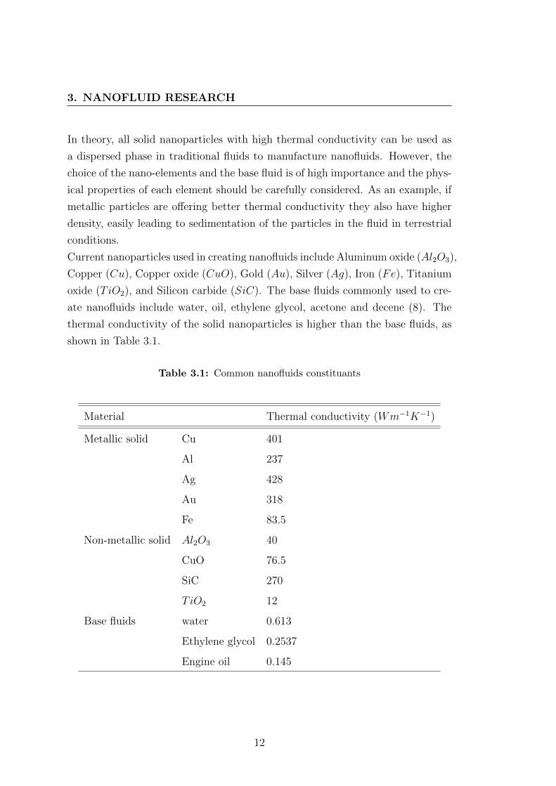
Current nanoparticles used in creating nanofluids include Aluminum oxide (Al2O3),
Copper (Cu), Copper oxide (CuO), Gold (Au), Silver (Ag), Iron (Fe), Titanium
oxide (TiO2), and Silicon carbide (SiC). The base fluids commonly used to cre-
ate nanofluids include water, oil, ethylene glycol, acetone and decene (8). The
thermal conductivity of the solid nanoparticles is higher than the base fluids, as
shown in Table 3.1.
Table 3.1: Common nanofluids constituants
Material Thermal conductivity (Wm−1K−1)
Metallic solid Cu 401
Al 237
Ag 428
Au 318
Fe 83.5
Non-metallic solid Al2O3 40
CuO 76.5
SiC 270
TiO2 12
Base fluids water 0.613
Ethylene glycol 0.2537
Engine oil 0.145
12
3.2 Literature review
3.2 Literature review
3.2.1 Applications
Except for the boiling heat and mass transfer applications, which comprise the
core of this research, nanofluids are widely studied for various applications. In
the field of heat transfer intensification, they show the potential for use in elec-
tronic applications, heat transportation, industrial cooling applications, heating
of buildings, as well as for cooling of nuclear systems. These applications are all
based on the potential increase of the thermal properties due to particle suspen-
sion into the base fluid.
Nanoparticles in suspension can be used in various applications such as solar
absorption, mechanical or biomedical applications. A few of them are described
below to give a short overview of some research into the nanofluid development.
In the biomedical domain, nanofluids can be used to deliver nanodrugs. When
drugs are delivered conventionally, the drug concentration increases in the pa-
tient’blood, reaches a peak and then drops when the drug is metabolized. By
using nanodrug delivery, the drug release can be more controlled, delivered over
a longer period and adapted to the therapeutic need. For example, gold nanopar-
ticles as shown by Ghosh et al. provide an effective means of drug delivery because
of their non toxicity and good interaction with thiols (9). Other biomedical appli-
cations on nanofluids include cancer therapeutics, antibacterial activity, sensing
and imaging, or cryopreservation.
Nanoparticles are also used for mechanical applications such as vehicular brake
fluids. During the braking phase, the kinetic energy of the vehicle is released
through the heat dispersed during the process and transmitted to the brake liquid.
Due to the improvement in each component of a vehicle, there is also a demand
for higher performance braking fluid. Copper and aluminum oxide based nanoflu-
ids have been produced for this purpose, and both show enhanced properties(10).
Their higher boiling point and viscosity decrease the risk of a vapour-lock that
would retard the hydraulic braking system to dissipate the heat, leading to en-
hancement of driving safety.
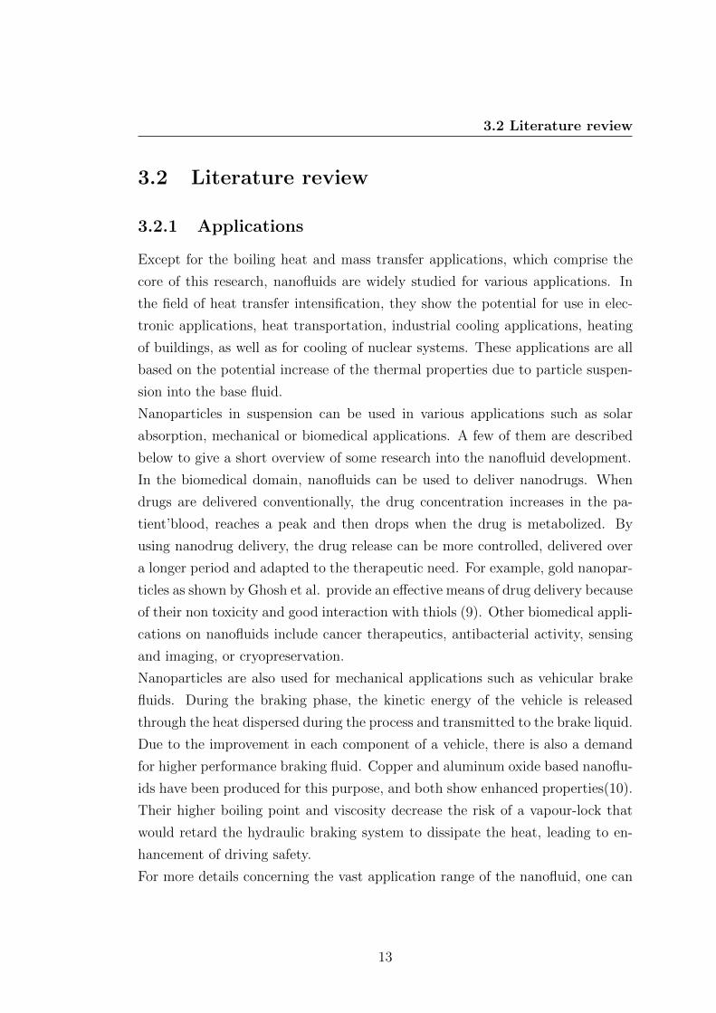
For more details concerning the vast application range of the nanofluid, one can
13
3. NANOFLUID RESEARCH
refer to the review article published by Wong and De Leon (11). Table 3.2 pro-
poses an overview of the properties of nanofluids and their potential applications.
Table 3.2: Nanoparticles applications
Properties/domain Applications example
Thermal heat and mass transfer
nuclear reactor cooling
heating of building
Optical surfaces with controlled refraction index
anti reflexion paint
Mechanical enhanced resistance to wear
anticorrosion properties
lighter, harder, more resistant composite materials
friction reduction
Magnetic enhancement of imaging
Electronic smaller components with higher capabilities
Biomedical drug delivery system
detection of desease
antibacterial band-aid
Environment waste water treatment
enhancement of green energy systems (solar panel)
Cosmetic efficient solar protection
14
3.2 Literature review
3.2.2 Preparation
The preparation of nanofluids is a major step in the use of nanoparticles for heat
transfer performance enhancement of fluids. Nanofluids are not simply binary
solid-liquid mixtures. There are several essential requirements into creating a
useful nanofluid including the stability of the fluids, minimal agglomeration of
the particles for a durable suspension, and no chemical change of the base fluid.
There are two main kinds of methods employed to produce nanofluids: the single-
step method and two-step method.
The single-step method involves the synthesis of the nanoparticles directly into
the liquid. Two main kinds of one-step method are currently used, the one-step
physical method and the one-step chemical method. With these methods the
nanoparticles are directly prepared by physical vapour deposition (PVD) or by
liquid chemical reaction.
The one single-step physical method was first developed by Akho et al. (12).
Eastman et al. has used a modified one-step physical technique in which solid
bulk copper was heated and vapourized then directly condensed into nanopar-
ticles via contact with a low flowing Ethylene Glycol (EG) vapour (13). The
prepared Cu − EG nanofluid was observed to contain particles with an average
size of less than 10 nm. Another physical one-step method, called Submerged Arc
Nanoparticles Synthesis System (SANSS), has been used by Lo et al. to prepare
various nanofluids containing CuO, TiO2, and Cu nanoparticles (14, 15) . The
particles are produced by heating the metal electrode (Cu, Ti) using arc sparking
and then condensing the vapour produced into the liquid in a vacuum chamber
to form nanofluids.
Zhu et al. have presented a novel single-step chemical method for preparing Cu-
EG nanofluids by reducing copper sulphate (CuSO4) with NaH2PO2 in ethylene
glycol under microwave irradiation (16). They also used the same kind of method
to produce CuO − water and Fe3O4 − water nanofluids (17, 18).
With these single-step methods, the processes of drying, storage, transportation
and dispersion of the nanoparticles are avoided. The agglomeration of the par-
ticles is then significantly reduced and the stability of the solution increased.
15
3. NANOFLUID RESEARCH
However, due to these methods and the properties of the nanofluid, only low
vapour pressure fluids are compatible with this process.
The two- steps method is a process where dry particles are dispersed into a base
liquid. Nanoparticles, nanotubes or nanofibres are first produced as dry particles
by different mechanisms such as inert gas condensation, chemical vapour depo-
sition, mechanical alloying or other suitable techniques. The obtained powder is
then dispersed into a base fluid which is considered to be the second step of the
process. For example, Eastman et al. and Lee et al. prepared Al2O3 − water
nanofluids using this method (13, 19). Hong prepared an Fe nanofluid by dispers-
ing Fe nanocrystaline powder in ethylene glycol by this two-step procedure (20).
As a result of this method, agglomeration of the particles may occur, especially
during the process of drying, storage and transportation. Such agglomerations
will conduct not only to settlement or clogging but also lead to a change in the
thermal properties of the prepared nanofluid. Different techniques, such as ul-
trasonic agitation, surfactant addition or pH control, can be used to avoid big
agglomeration and improve the dispersion behaviour (8). Nanoparticle powder
synthesis techniques have already been used industrially by several industrial
companies, thus demonstrating economic advantages in using a two-step method,
using these powders. But the key issue for the dispersion two-step method is the
breaking of agglomerations and the prevention of re-aggregation of nanoparticles.
Moreover, the two-step technique, as compared to the one-step method, is usually
used for the preparation of non-metallic nanofluids.
3.2.3 Stabilization
One major limitation of the use of a nanofluid as a heat transfer fluid is its stabil-
ity. There are two phenomena that are critical for the stability of the nanofluid:
sedimentation and aggregation. The Stokes law, as used by Hiemenz, governs the
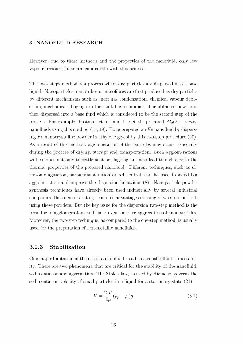
sedimentation velocity of small particles in a liquid for a stationary state (21):
V =2R2
9µ(ρp − ρl)g (3.1)
16
3.2 Literature review
where, V is the sedimentation velocity of particles, R is the radius of the particles,
µ is the viscosity of the base fluid, ρp and ρl are the density of the particles and
the liquid, respectively, and g is the gravitational acceleration. According to this
equation, measures to reduce the sedimentation velocity and therefore increase
the stability of the nanofluid can include:
• reducing the size of the nanoparticles
• increasing the viscosity of the base fluid
• reducing the density difference between the nanoparticles and the base fluid
Increasing the viscosity of the base fluid or reducing the density difference is not
appropriate for heat transfer application since the nanoparticles and the base
fluid are first chosen for their thermal and physical properties. It is clear that
reducing the particle size will decrease the sedimentation velocity. According to
theory in colloid chemistry, the sedimentation will stop when the particles reach
a critical size due to the Brownian motion of nanoparticles (21). At this point,
the nanoparticles reach the equilibrium between sedimentation and diffusion. Al-
though equilibrium is reached, the smaller nanoparticles have higher surface en-
ergy and increase the probability of the aggregation between the particles. For
normal gravity applications, the key to preparing nanofluids is to use particles
as small as possible and prevent aggregation physically and/or chemically (for
example, by using appropriate surfactants to separate the nanoparticles).
As discussed previously, the key to the stability of the nanofluids, is the size of
the nanoparticles. One should avoid agglomeration of the nanoparticles. There
are several ways to prevent this process and then enhance the stability of the
nanofluids.
As explained previously, the two-step method allows easy and fast preparation
of nanopowder but also induces an easier agglomeration of the particles during
the drying process. When dispersed into the base fluid, and after sonication to
break the agglomerates, the particles keep agglomerating because of the Van Der
Waals forces. Some products, known as surfactants or dispersant when used for
17
3. NANOFLUID RESEARCH
nanofluids, need to be added to avoid the agglomeration. Two concepts are usu-
ally used, steric barrier or charge stabilization. They find their justification in
the interaction between particle theory.
When dispersed in the base fluid, the particles are subject to molecular inter-
actions such as collision between fluid and particle atoms, the Brownian motion
but also unwanted interactions as Van Der Waals forces low range electrostatic
interaction, or other ionic interaction. These last phenomena have a disastrous
effect on the colloid stability; large packets of material will flocculate quickly re-
ducing the effectiveness of the nanofluid. This phenomenon is well explained by
Derjaguin Landau,Verwey Overbeek (DLVO) theory. This theory suggests that
the stability of a dispersion of colloids depends on the total potential energy, a
combination of attractive, repulsive and solvent energy. The DLVO theory will
not be described here, but based on it, a possible way to enhance the stability
of the nanofluids is to induce repulsive forces, stronger than the Van Der Waals
forces. The first approach into doing so, is to induce electrostatic repulsive forces.
The nanoparticles will have their surfaces charged electricaly because of the ions
provided by the dispersant. As a result, the particles will repulse each other be-
cause they are electrically charged identically. However, this electrostatic repul-
sive forces reposes on ionic stability: if during the life of the nanofluids, more ions
are added or if the pH is modified, this electric barrier could become ineffective,
leading to a dominance of the Van Der Waals forces and then to re-agglomeration
of the particles.
Another way to stabilize the nanofluid and to avoid agglomeration of the parti-
cles is to use a physical barrier between the particles, also called a steric barrier.
To establish this barrier, polymeric materials of several nanometres of thickness
hydroxyl-propyl cellulose or polyethylene glycol are usually used and can be added
to the dispersion. These polymers will fix themselves onto the colloid surface low-
ering the entropy of the system and the close contact of two particles will become
thermodynamically unfavourable. Also, an osmotic pressure will be formed be-
tween particles and will draw liquid into the space between them and force the
particles apart. However, adding too many polymers could have a contrary ef-
fect as they would create bridges between the particles if all their surfaces were
already taken.
18
3.2 Literature review
Equation 3.1 shows the potential effectiveness of nanofluids for reduced grav-
ity applications. Actually the main limitation is the stability depending on the
sedimentation velocity which, theoretically, tends to become zero when the grav-
itational acceleration tends to zero. The effectiveness of nanofluids in reduced
gravity then only relies on the heat transfer efficiency, which is the main purpose
of this study.
3.2.4 Nanofluids properties: Thermal conductivity
The thermal conductivity is the most important parameter that can improve the
heat transfer characteristics of a nanofluid. Different techniques are usually used
to determine the thermal conductivity of nanofluid and include the transient
hot-wire method , optical beam-deflection method or the steady state parallel
plate technique (22, 23, 24). Other methods exist but among them, the transient
hot wire method is the most commonly used. It works by measuring the time
response to a sharp temperature pulse. A derivation of Fourrier’s law and the
temperature measurements are used to determine the thermal conductivity. The
review of available literature on the thermal conductivity with nanofluid shows
that only a small volumic concentration of particles can significantly increase this
parameter (25). Generally, thermal conductivity increases with the increase in
the concentration of nanoparticles. This is confirmed by all the data found in the
literature. The issues are the mechanisms responsible for the thermal conductiv-
ity enhancement.
In most research, the enhancement in thermal conductivity is linear and only
depends on the volume fraction of particles. Lee et al. obtained an increase
by 10% for Al2O3-water nanofluid at 4 vol% and an increase by 12% for CuO-
water at 3.5 vol% (the size of the particles was 23.6nm)(19). This corresponds to
a normal increase in the thermal conductivity that could be predicted using the
two-phase mixture theory. More than a century ago, Maxwell proposed a method
to determine the thermal conductivity of a solid/liquid mixture made of spherical
particles (26):
19
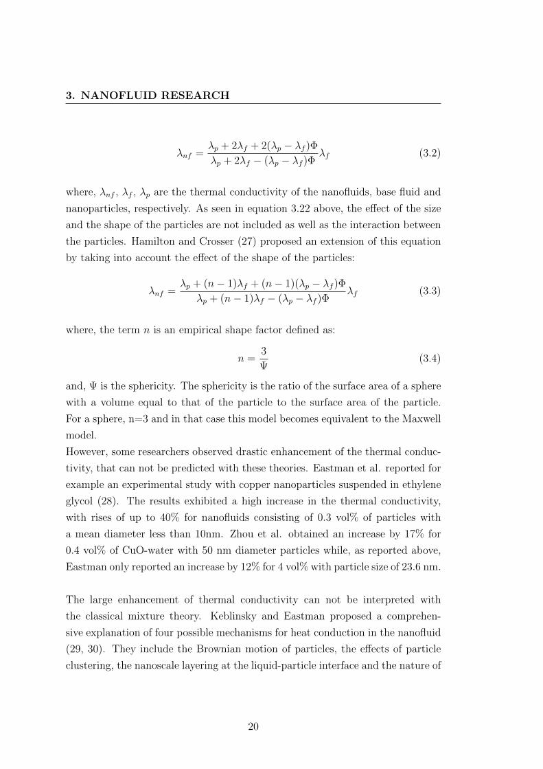
3. NANOFLUID RESEARCH
λnf =λp + 2λf + 2(λp − λf )Φλp + 2λf − (λp − λf )Φ
λf (3.2)
where, λnf , λf , λp are the thermal conductivity of the nanofluids, base fluid and
nanoparticles, respectively. As seen in equation 3.22 above, the effect of the size
and the shape of the particles are not included as well as the interaction between
the particles. Hamilton and Crosser (27) proposed an extension of this equation
by taking into account the effect of the shape of the particles:
λnf =λp + (n− 1)λf + (n− 1)(λp − λf )Φ
λp + (n− 1)λf − (λp − λf )Φλf (3.3)
where, the term n is an empirical shape factor defined as:
n =3
Ψ(3.4)
and, Ψ is the sphericity. The sphericity is the ratio of the surface area of a sphere
with a volume equal to that of the particle to the surface area of the particle.
For a sphere, n=3 and in that case this model becomes equivalent to the Maxwell
model.
However, some researchers observed drastic enhancement of the thermal conduc-
tivity, that can not be predicted with these theories. Eastman et al. reported for
example an experimental study with copper nanoparticles suspended in ethylene
glycol (28). The results exhibited a high increase in the thermal conductivity,
with rises of up to 40% for nanofluids consisting of 0.3 vol% of particles with
a mean diameter less than 10nm. Zhou et al. obtained an increase by 17% for
0.4 vol% of CuO-water with 50 nm diameter particles while, as reported above,
Eastman only reported an increase by 12% for 4 vol% with particle size of 23.6 nm.
The large enhancement of thermal conductivity can not be interpreted with
the classical mixture theory. Keblinsky and Eastman proposed a comprehen-
sive explanation of four possible mechanisms for heat conduction in the nanofluid
(29, 30). They include the Brownian motion of particles, the effects of particle
clustering, the nanoscale layering at the liquid-particle interface and the nature of
20
3.2 Literature review
heat transport in the nanoparticles. From their investigations, it was shown that
the movement of the nanoparticles due to the Brownian motion was very slow in
transporting large amounts of heat through nanofluids. They demonstrated that
the clustering of particles led to negative effects on the thermal conductivity en-
hancement, the increase being higher for loosely packed clusters than for closely
packed ones. And from a nanolayer of liquid at the liquid-particle interface, a
higher thermal conductivity can be obtained.
The mechanisms of thermal conductivity enhancement is a hotly debated topic,
since some studies reported high increase in thermal conductivity with a small
load of nanoparticles and other showed normal increase in thermal conductivity,
according to the well-established medium theory exposed before. Li et al and
Keblinski et al. proposed good reviews of the past and on-going research and
presented the different opposing theories and controversies on the thermal con-
ductivity enhancement of nanofluids (8, 31).
21
3. NANOFLUID RESEARCH
3.3 Experimental HFE7000-Al2O3 nanofluids
Preparing a stable nanofluid is a prerequisite in order to enhance and optimize its
thermal characteristics for use as heat transfer fluid. As explained before, many
combinations of material can be used. These include nanoparticles of metals or
oxide such as titanium oxide, aluminum oxide, copper and lead, dispersed into
water, ethanol, ethylene glycol or any type of refrigerant. Some of these different
combinations have been prepared and tested (TiO2 in water, Al2O3 in water or
ethanol) but are not presented in this report. However, the following sections
present the preparation and characterisation of the main nanofluid that was used
in this work. It is made of HFE 7000 (1-methoxyheptafluoropropane) as a base
fluid, where nanoparticles of aluminum oxide have been dispersed.
3.3.1 Preparation
The preparation and characterization of the nanofluid is a key step in this study.
For the purposes of this research, experiments will be carried out using HFE-
7000 manufactured by 3M as a base fluid because of its physical properties such
as being odorless, nonflammable, non-explosive, semi-transparent in the infrared
wavelengths, and having low phase change enthalpy and low boiling temperature.
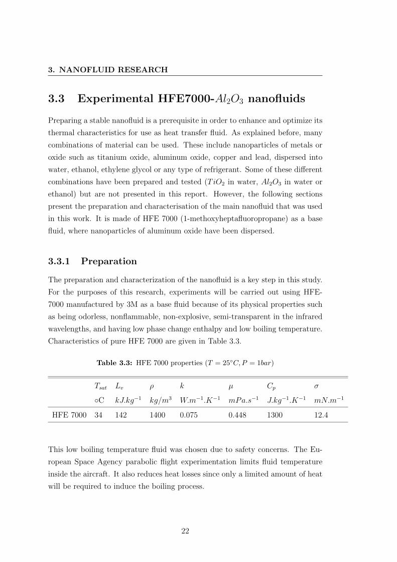
Characteristics of pure HFE 7000 are given in Table 3.3.
Table 3.3: HFE 7000 properties (T = 25C,P = 1bar)
Tsat Lv ρ k µ Cp σ
C kJ.kg−1 kg/m3 W.m−1.K−1 mPa.s−1 J.kg−1.K−1 mN.m−1
HFE 7000 34 142 1400 0.075 0.448 1300 12.4
This low boiling temperature fluid was chosen due to safety concerns. The Eu-
ropean Space Agency parabolic flight experimentation limits fluid temperature
inside the aircraft. It also reduces heat losses since only a limited amount of heat
will be required to induce the boiling process.
22
3.3 Experimental HFE7000-Al2O3 nanofluids
The selection of the nanoparticles is based on the size, shape and thermal prop-
erties of the material. Spherical or nearly spherical nanoparticles with a diameter
between 25 and 100 nm have been nominated for this research. In this investiga-
tion, Al2O3 nanoparticles were selected because of their well documented thermal
properties and wide spread use in the research community. Dry nanoparticles were
purchased from US Research Nanomaterials, Inc.. The properties given by the
suppliers are given in Table 3.4.
Table 3.4: Al2O3 nanoparticles properties given by the supplier
Purity APS Grain size SSA Morphology Crystal structure
Al2O3 99+% 80 nm 27 nm > 15m2/g nearly spherical rhombohedral
where, APS is the average particle size and SSA is the specific surface area.
The particles are then dispersed into the base fluid. Because the nanoparticles
are supplied in powder form, dry, agglomeration of the particles is unavoidable.
The mixture is sonicated using an ultrasonic bath for approximately 8 hours and
Triton X114 is added as a surfactant. After the sonication, it was observed that
it was not possible to break all the particle agglomerations. The mixtures were
filtrated using a 200 nm filter.
Due to the filtration, the concentrations of the nanofluids needed to be measured.
After evaporation of 20 g of the mixture, the weight of the deposited particles
was measured. The prepared mixtures were then diluted to obtain nanofluids at
0.1, 0.5 and 1% concentration in mass (wt%) . However, most of the studies and
correlations are based on the volumic fraction of nanoparticles. The determina-
tion of the volumic fraction of particles, knowing the weight fraction, is as follows:
Φv =Φm
Φm + ρpρf
(1− Φm)(3.5)
where, Φv and Φm are the volumic and mass fraction, respectively, and ρp and
23
3. NANOFLUID RESEARCH
ρf are the particles and fluid density, respectively. According to these equations,
0.1, 0.5 and 1 wt% lead to 0.036, 0.18 and 0.36 vol%, respectively.
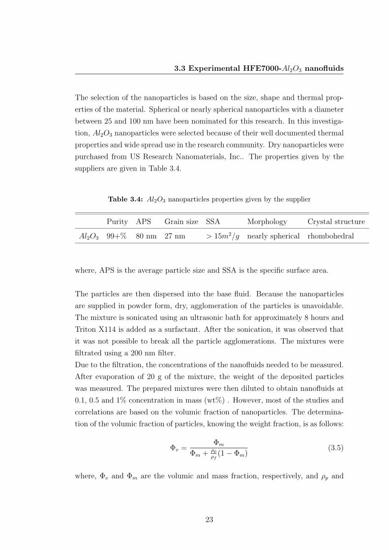
The prepared nanofluids, shown in Figure 3.1, were left to rest and stored in the
fridge. They were found to be very stable. After one week, no deposition was ob-
served. A light deposition of particles started to be observed after approximately
three months.
Figure 3.1: Photograph of the prepared nanofluids showing increasing weight
percentages of Al2O3 in HFE7000.
3.3.2 Characterization
The thermo-physical and colloidal properties of the prepared nanofluids need
to be measured to ensure that they are different from the base fluid and well
characterized. For that purpose, the colloid density, vapour density, viscosity,
surface tension, specific heat capacity and the thermal conductivity need to be
investigated. These measured values will then be compared to the existing models
described below. Nanoparticles size and agglomerations will also be characterized
as well as some optical properties.
24
3.3 Experimental HFE7000-Al2O3 nanofluids
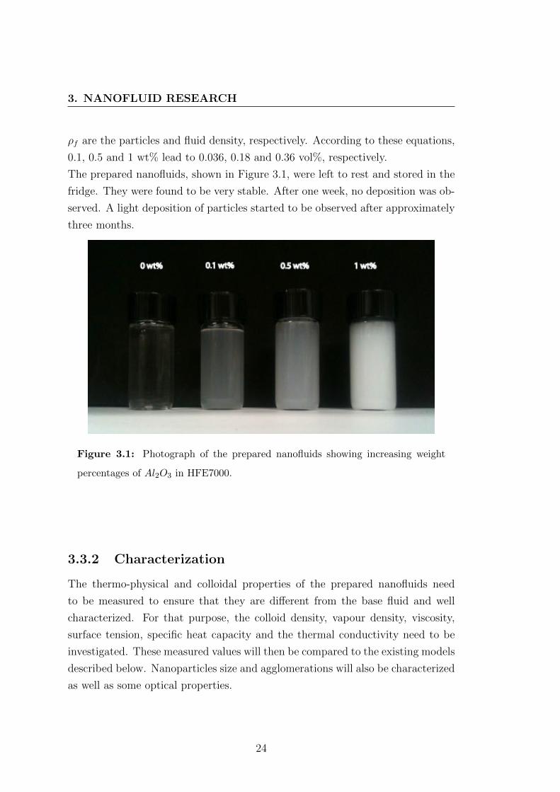
3.3.2.1 Particle size
Because the nanofluids were prepared using a two-step method, the size of the
particles dispersed into the base fluid is probably different to the size claimed by
the supplier. It is proposed that the use of the ultrasonic bath did not break all
the particle agglomerations. The size distribution of the particles was determined
using dynamic light scattering (DLS). The Brownian motion of particles dispersed
in the liquid causes laser light to be scattered at different intensities. Analysis of
these intensity variations leads to the determination of the particle size using the
Stokes-Einstein relationship. In this study, a MALVERN DLS was used. Mea-
surements were repeated three times to minimize the calculation errors. Figure
3.2 presents the size distribution of our prepared nanofluids. The representation
in number of the results shows that the average particles size is 150nm with a dis-
tribution peak at 140nm. This result shows a big difference between the nominal
size of the particles (80 nm) and the actual size of the particle or particles ag-
glomeration in the base fluid. Nevertheless, a size of 140 nm is acceptable for our
study since the prepared nanofluids remained stable for more than three months.
Figure 3.2: Size distribution of Al2O3 nanoparticles in HFE7000.
25
3. NANOFLUID RESEARCH
3.3.2.2 Density
Calculation of the effective density of nanofluid is straightforward. It can be
estimated using the physical principle of the mixture rule:
ρnf =m
V=mf +mp
Vf + Vp=ρfVf + ρpVpVf + Vp
= (1− Φ)ρf + Φρp (3.6)
where, ρnf , ρf , ρp are the density of the nanofluids, base fluid and nanoparticles,
respectively, and Φ is the volume fraction of particles. Since this study is mostly
focussed on the effect of low concentration of nanoparticles (0-5%), the resulting
density of the prepared nanofluids is expected to be quite similar to the density
of the base fluid. The density of the samples is measured using a pycnometer.
The volume capacity of the pycnometer being precisely known, it just needs to
be weighted with a Metler Toledo precision balance before and after filling, which
leads to the easy calculation of the density of our nanofluids. The measurements
were repeated five times for each sample to limit the experimental errors.
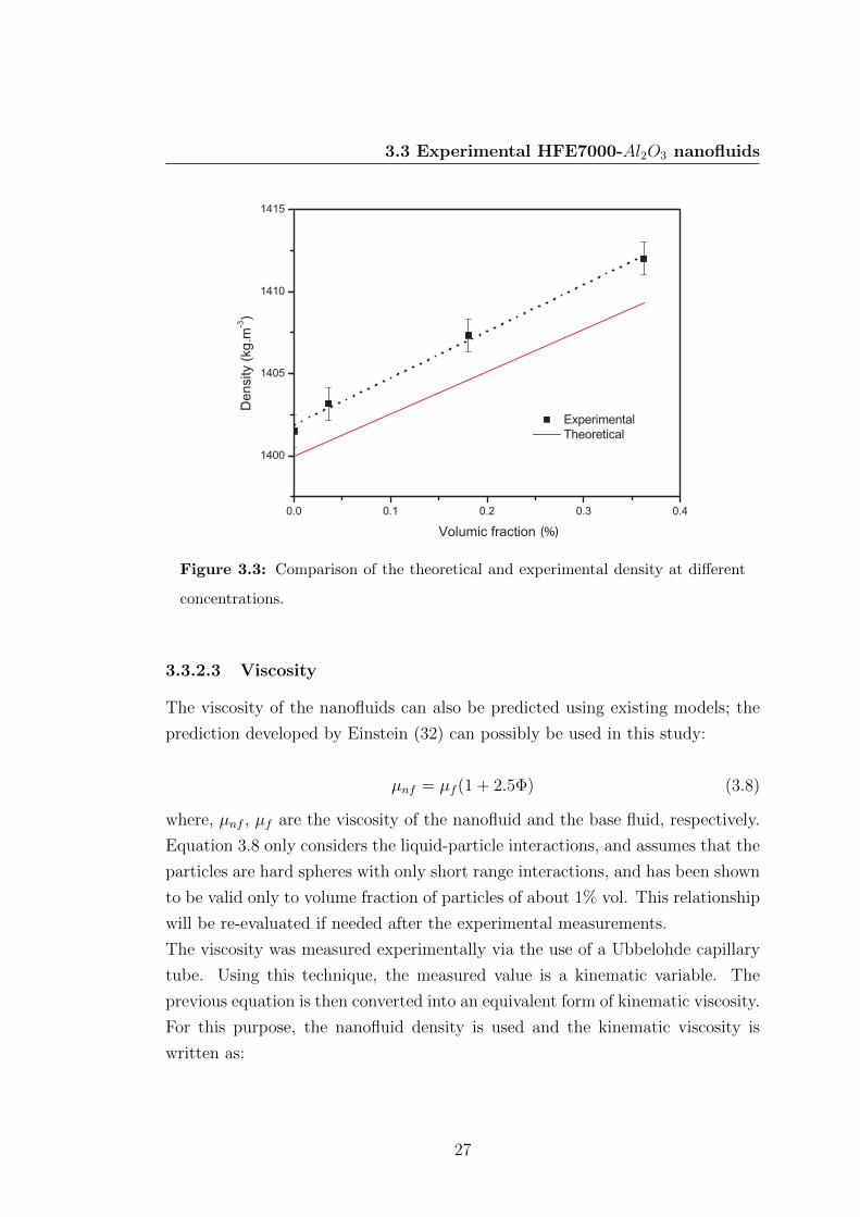
The results are shown in Figure 3.3, where the density is plotted versus the
volumic fraction and compared to the theoretical density calculated with equation
3.6.
There is a 0.2 % difference between the experimental and theoretical density and
as expected, the density of our nanofluids is similar to the density of the base
fluid (for the highest concentration, i.e. 1 wt%, the density difference is less than
0.9 % as compared to the base fluid). Additionally, Figure 3.3, shows the mixture
theory to be valid for the density determination of low concentration nanofluids,
theoretical and experimental curves showing the same trend.
If we assume that the particles as are as volatile as the liquid particles, the vapour
density of the nanofluids can be calculated as:
ρnf,v = ρvΦρp + (1− Φ)ρfΦρv + (1− Φ)ρf
(3.7)
26
3.3 Experimental HFE7000-Al2O3 nanofluids
(%)
Figure 3.3: Comparison of the theoretical and experimental density at different
concentrations.
3.3.2.3 Viscosity
The viscosity of the nanofluids can also be predicted using existing models; the
prediction developed by Einstein (32) can possibly be used in this study:
µnf = µf (1 + 2.5Φ) (3.8)
where, µnf , µf are the viscosity of the nanofluid and the base fluid, respectively.
Equation 3.8 only considers the liquid-particle interactions, and assumes that the
particles are hard spheres with only short range interactions, and has been shown
to be valid only to volume fraction of particles of about 1% vol. This relationship
will be re-evaluated if needed after the experimental measurements.
The viscosity was measured experimentally via the use of a Ubbelohde capillary
tube. Using this technique, the measured value is a kinematic variable. The
previous equation is then converted into an equivalent form of kinematic viscosity.
For this purpose, the nanofluid density is used and the kinematic viscosity is
written as:
27
3. NANOFLUID RESEARCH
νnf =µnfρnf
(3.9)
The measurement principle is quite simple. Once the reservoir is filled, the liquid
goes through the capillary tube. When the fluid reaches measurement mark one,
the time taken to reach measurement mark two and the time to mark three are
measured. The number of seconds obtained between two measurement marks
gives directly the kinematic viscosity by multiplying by a constant C, given by
the fabricant and depending on the capillary tube:
ν = C(t− τ) (3.10)
where, t is the time in seconds and τ is a time correction depending on the cap-
illary tube, and given by the supplier.
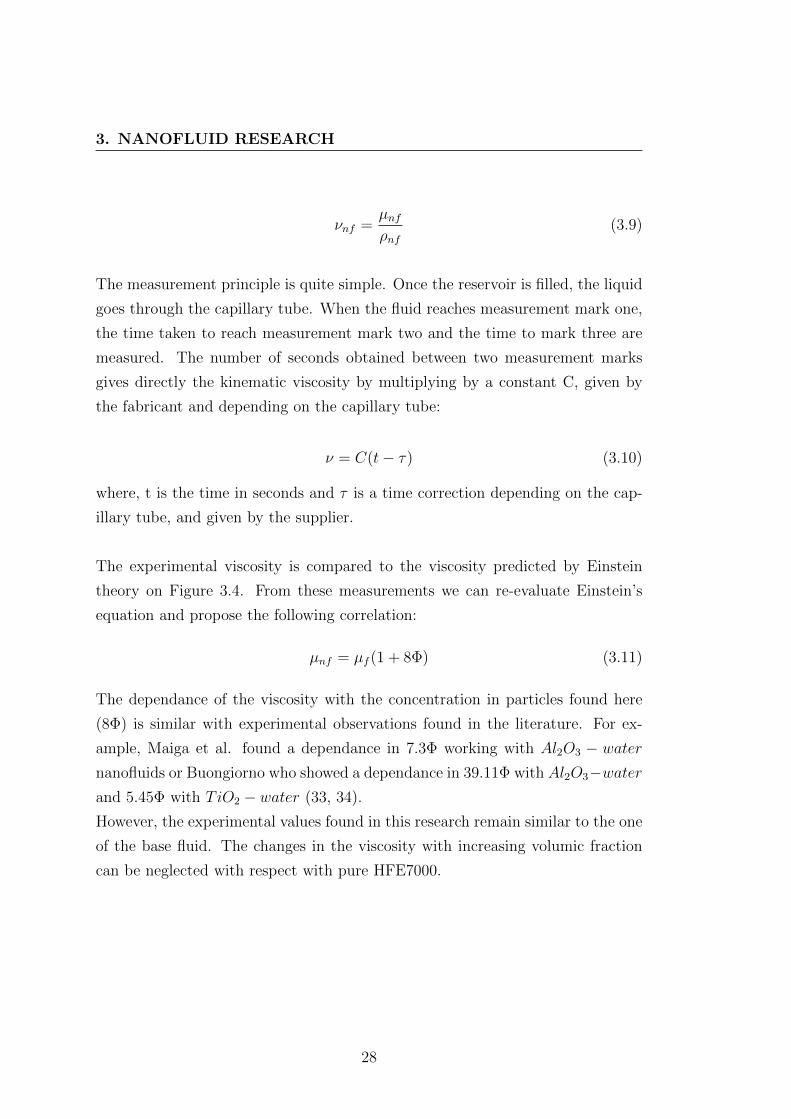
The experimental viscosity is compared to the viscosity predicted by Einstein
theory on Figure 3.4. From these measurements we can re-evaluate Einstein’s
equation and propose the following correlation:
µnf = µf (1 + 8Φ) (3.11)
The dependance of the viscosity with the concentration in particles found here
(8Φ) is similar with experimental observations found in the literature. For ex-
ample, Maiga et al. found a dependance in 7.3Φ working with Al2O3 − water
nanofluids or Buongiorno who showed a dependance in 39.11Φ with Al2O3−waterand 5.45Φ with TiO2 − water (33, 34).
However, the experimental values found in this research remain similar to the one
of the base fluid. The changes in the viscosity with increasing volumic fraction
can be neglected with respect with pure HFE7000.
28
3.3 Experimental HFE7000-Al2O3 nanofluids
(%)
Figure 3.4: Comparison of the theoretical and experimental viscosity at different
concentrations.
3.3.2.4 Specific heat
The specific heat capacity is one of the important thermal properties that will
affect the thermal performances of the nanofluid. It can be calculated using the
same theory of mixtures used to determine the density. This theory of mixture
theory yields:
Cp,nf = (1− Φ) Cp,f + ΦCp,p (3.12)
where, Cp,nf , Cp,f ,Cp,p are the specific heat capacity of the nanofluids, base fluid
and nanoparticles, respectively. However, this equation does not properly agree
with some experimental results as shown by Zhou and Ni (35). They recom-
mended another expression for the specific heat capacity of a liquid/solid mixture
which agrees well with their data as shown by equation 3.13. Thermal equilib-
rium can be assumed between the nanoparticles and the base fluid due to the
extremely small size of the particles and, therefore, the heat capacity becomes:
29

3. NANOFLUID RESEARCH
Cp,nf =(1− Φ)ρfCp,f + ΦρpCp,p
(1− Φ)ρf + Φρp(3.13)
The value of the specific heat will need to be measured to evaluate if the presented
models are suitable for the nanofluids used in this study with respect to different
working concentrations. For this purpose, a Differential Scanning Calorimeter
(DSC) is used to measure the specific heat of a solution. Differential Scanning
Calorimetry is a technique in which the difference in the amount of heat required
to increase the temperature between the sample and a reference is measured as
a function of the temperature, leading to the calculation of the specific heat.
Due to the volatility of HFE 7000, measurements with the DSC are relatively
complicated and are on-going in another laboratory. However, it is expected that
the specific heat capacity of the prepared nanofluids will be closely similar to
the one of the base fluid. Actually, by using equation 3.13, the specific heat
difference as compared to the base fluid can be calculated. It gives, for the most
concentrated nanofluid at 1 wt%, a specific heat of 1295.8 J.kg−1.K−1, which
represents a drop by only approximately 0.32% as compared to pure HFE7000.
The specific heat capacity of the prepared nanofluids will then be considered to
be equivalent to the pure HFE7000 specific heat capacity.
3.3.2.5 Surface tension
The surface tension is a measurement of the cohesive energy present at an inter-
face, and plays an important role in boiling phenomena. For this research, it is
imperative to measure the surface tension of the nanofluids since it is affected by
surfactants, chemicals, and residual dust. Traditional methods to determine the
surface tension include the Du Nouy Ring method or the Wilhelmy plate method
(36). In order to obtain fast measurements, one possible method is to use a cap-
illary method. In a capillary tube, a liquid rises until a height, H, where the
liquid pressure just under the meniscus is controlled by the hydrostatic law and
the Young-Laplace equation. By combining these two laws and their resulting
30
3.3 Experimental HFE7000-Al2O3 nanofluids
equations, the Jurin’s equation is obtained:
H =2σcosθ
rgρf(3.14)
where, H is the height reached by the liquid, r is the radius of the capillary tube
(which should be less than the capillary length of the fluid) and θ is the contact
angle between the tube and the liquid at the meniscus (in practice, it is assumed
that the fluid is fully wetting the surface, θ = 0).
The measurements were repeated five times for each concentration, and the results
shown below in Figure 3.5. The averaged values of the measured surface tension
show that the change of surface tension for low concentration of nanoparticles, as
compared with pure liquid, is not significant. However, one can notice that in the
same manner as the results presented in the literature (37), the surface tension
is slightly increased with the increase of the particle concentrations, as compared
with the base fluid. This could be explained by the Van der Waals forces. With
the increase of the concentration, the nanoparticles get closer to each other and
could be accumulated at the liquid-vapour interface, increasing the Van der Waals
forces leading to the rise of the surface free energy and increasing the surface
tension.
In a trial to obtain more precise measurements, the Pendant drop method was
performed to determine surface and interfacial tension by optical visualization and
analyzed by using the FTA 200 device (36). This method suspends a drop by a
thin needle and surface tension is determined by fitting the shape of the drop (in a
captured video image as seen of Figure 3.6) to the Young-Laplace equation which
relates interfacial tension to drop shape (a software does this automatically).
Because of the volatility of the base fluid, measurements of the surface tension
using this technique require particular care. To avoid material loss by evaporation
during the process, it is required to obtain a environment saturated in HFE7000.
Surface tension measurements using this technique are shown on Figure 3.5, and
present similar results as with the capillary method. The variation between the
two methods is mainly due to the difficulty in the measurement. The surface
tension of HFE7000, being low as compared to classical fluids, such as water,
even small impurity will affect the obtained value. However, the changes in
31
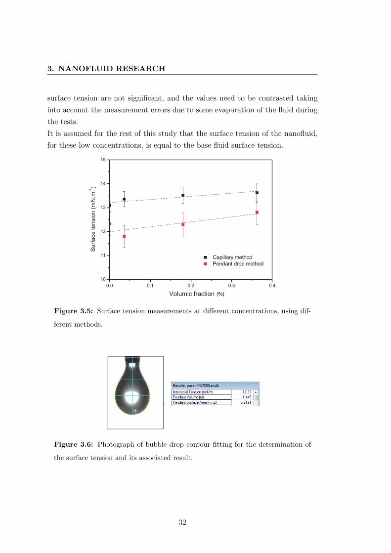
3. NANOFLUID RESEARCH
surface tension are not significant, and the values need to be contrasted taking
into account the measurement errors due to some evaporation of the fluid during
the tests.
It is assumed for the rest of this study that the surface tension of the nanofluid,
for these low concentrations, is equal to the base fluid surface tension.
(%)
Figure 3.5: Surface tension measurements at different concentrations, using dif-
ferent methods.
Figure 3.6: Photograph of bubble drop contour fitting for the determination of
the surface tension and its associated result.
32
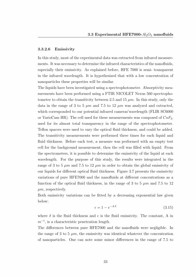
3.3 Experimental HFE7000-Al2O3 nanofluids
3.3.2.6 Emissivity
In this study, most of the experimental data was extracted from infrared measure-
ments. It was necessary to determine the infrared characteristics of the nanofluids,
especially their emissivity. As explained before, HFE 7000 is semi- transparent
in the infrared wavelength. It is hypothesized that with a low concentration of
nanoparticles these properties will be similar.
The liquids have been investigated using a spectrophotometer. Absorptivity mea-
surements have been performed using a FTIR NICOLET Nexus 560 spectropho-
tometer to obtain the transitivity between 2.5 and 15 µm. In this study, only the
data in the range of 3 to 5 µm and 7.5 to 12 µm was analyzed and extracted,
which corresponded to our potential infrared cameras’wavelength (FLIR SC6000
or VarioCam HR). The cell used for these measurements was composed of CaF2,
used for its almost total transparency in the range of the spectrophotometer.
Teflon spacers were used to vary the optical fluid thickness, and could be added.
The transitivity measurements were performed three times for each liquid and
fluid thickness. Before each test, a measure was performed with an empty test
cell for the background measurement, then the cell was filled with liquid. From
the spectrometers, it is possible to determine the emissivity of the liquid at each
wavelength. For the purpose of this study, the results were integrated in the
range of 3 to 5 µm and 7.5 to 12 µm in order to obtain the global emissivity of
our liquids for different optical fluid thickness. Figure 3.7 presents the emissivity
variations of pure HFE7000 and the nanofluids at different concentrations as a
function of the optical fluid thickness, in the range of 3 to 5 µm and 7.5 to 12
µm, respectively.
Both emissivity variations can be fitted by a decreasing exponential law given
below:
ε = 1− e−A.δ (3.15)
where δ is the fluid thickness and ε is the fluid emissivity. The constant, A in
m−1, is a characteristic penetration length.
The differences between pure HFE7000 and the nanofluids were negligible. In
the range of 3 to 5 µm, the emissivity was identical whatever the concentration
of nanoparticles. One can note some minor differences in the range of 7.5 to
33
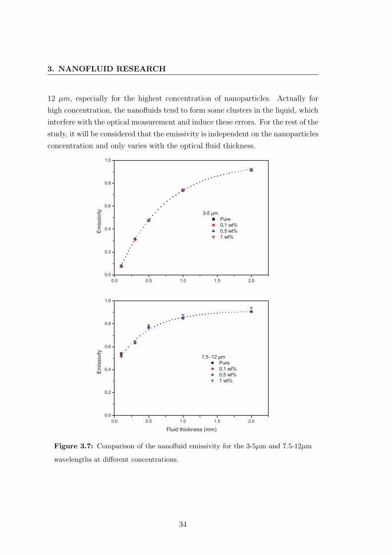
3. NANOFLUID RESEARCH
12 µm, especially for the highest concentration of nanoparticles. Actually for
high concentration, the nanofluids tend to form some clusters in the liquid, which
interfere with the optical measurement and induce these errors. For the rest of the
study, it will be considered that the emissivity is independent on the nanoparticles
concentration and only varies with the optical fluid thickness.
Figure 3.7: Comparison of the nanofluid emissivity for the 3-5µm and 7.5-12µm
wavelengths at different concentrations.
34
3.3 Experimental HFE7000-Al2O3 nanofluids
3.3.2.7 Thermal conductivity
Many studies on the thermal conductivity of nanofluids have been carried out
using the well-known hot wire method, consisting of measuring the temperature
rise in the fluid at a defined distance from a linear heat source (hot wire). It
seems that this method is not adapted to nanofluid thermal conductivity mea-
surement because of the possible particle deposition on the hot wire, resulting in
discrepancies in the results.
In the method presented here, developed in collaboration with Dr. Jean-Laurent
Gardarein (IUSTI), the determination of the thermal conductivity was made by
the measurement of the thermal diffusivity of the nanofluids. It used a classi-
cal characterization method, which consisted of heating the sample on one side
and measuring the temperature on the opposite side. The appropriate model,
partially described here, gives a precise estimation of the thermal diffusivity, and
then of the thermal conductivity.
Experimental set-up:
A 4mm layer of the liquid was trapped in a cylindrical cell closed by two
thin aluminum plates (1mm). The main axis of the cell was directed along the
gravity axis and the heated surface is the upper face, in order to stratify the liq-
uid and prevent convective heat transfer. The heating device was a light emitting
in the visible and infrared wavelengths. The upper aluminum face was painted
in black to increase its absorptivity. The temperature measurement was made
on the lower aluminum face with a 0.5mm thermocouple. Figure 3.8 presents a
schematic of the experiment.
The heating period depends on the samples to be tested and is determined to
obtain a significant and measurable increase in the temperature (however the
heating time has to be limited). The heating period and the initial heating time
need to be precisely known. For that purpose, one can use a photodiode or place
a thermocouple on the black cell. A reflective mask was also added between the
cell and the lamp in order to only heat the black painted aluminum face placed
above the fluid to be characterized. The following Figure 3.9, shows a typical
signal obtained with this method.
35
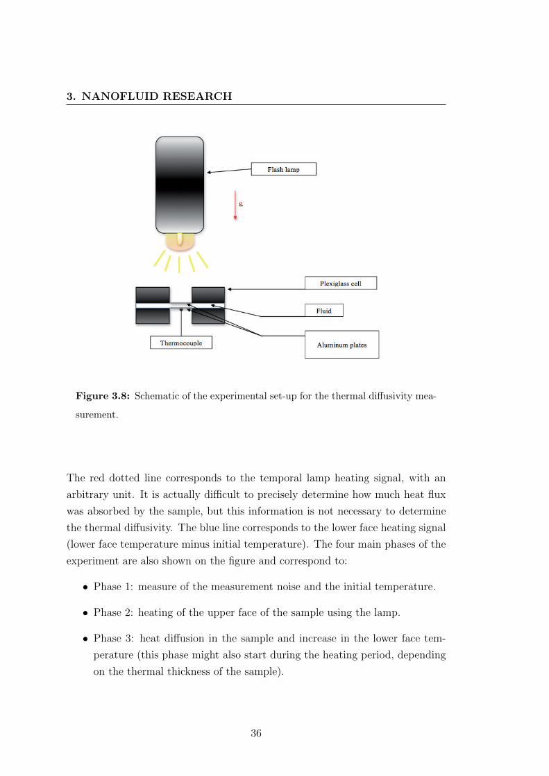
3. NANOFLUID RESEARCH
Figure 3.8: Schematic of the experimental set-up for the thermal diffusivity mea-
surement.
The red dotted line corresponds to the temporal lamp heating signal, with an
arbitrary unit. It is actually difficult to precisely determine how much heat flux
was absorbed by the sample, but this information is not necessary to determine
the thermal diffusivity. The blue line corresponds to the lower face heating signal
(lower face temperature minus initial temperature). The four main phases of the
experiment are also shown on the figure and correspond to:
• Phase 1: measure of the measurement noise and the initial temperature.
• Phase 2: heating of the upper face of the sample using the lamp.
• Phase 3: heat diffusion in the sample and increase in the lower face tem-
perature (this phase might also start during the heating period, depending
on the thermal thickness of the sample).
36
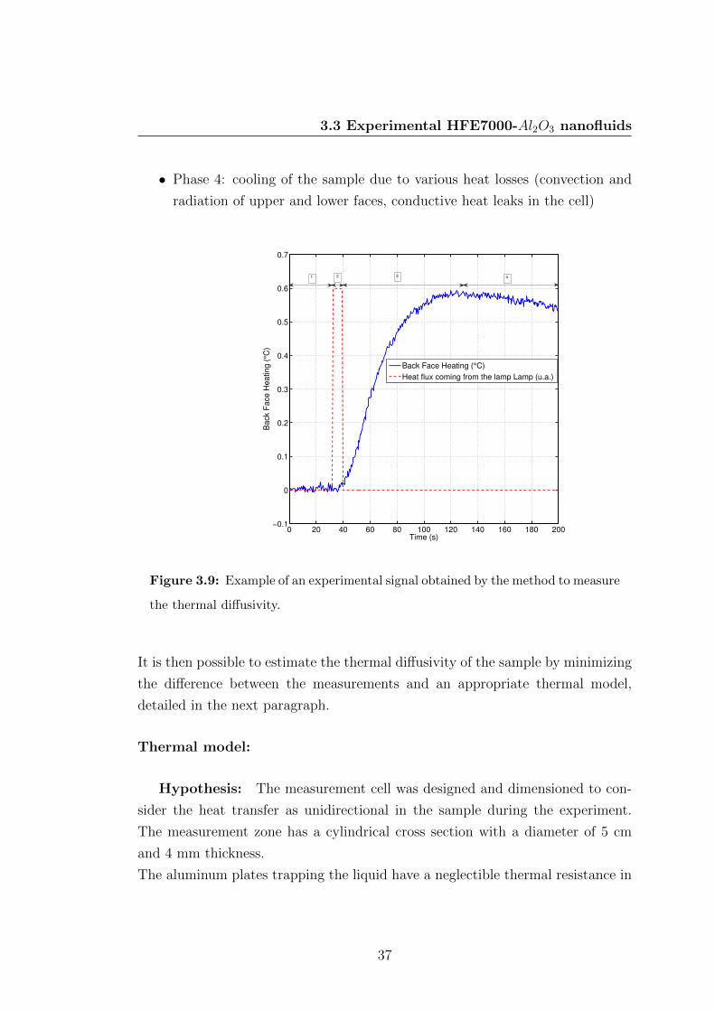
3.3 Experimental HFE7000-Al2O3 nanofluids
• Phase 4: cooling of the sample due to various heat losses (convection and
radiation of upper and lower faces, conductive heat leaks in the cell)
0 20 40 60 80 100 120 140 160 180 200−0.1
0
0.1
0.2
0.3
0.4
0.5
0.6
0.7
Time (s)
Back F
ace H
ea
ting (
°C)
Back Face Heating (°C)
Heat flux coming from the lamp Lamp (u.a.)
1 2 3 4
Figure 3.9: Example of an experimental signal obtained by the method to measure
the thermal diffusivity.
It is then possible to estimate the thermal diffusivity of the sample by minimizing
the difference between the measurements and an appropriate thermal model,
detailed in the next paragraph.
Thermal model:
Hypothesis: The measurement cell was designed and dimensioned to con-
sider the heat transfer as unidirectional in the sample during the experiment.
The measurement zone has a cylindrical cross section with a diameter of 5 cm
and 4 mm thickness.
The aluminum plates trapping the liquid have a neglectible thermal resistance in
37
3. NANOFLUID RESEARCH
front of the liquid (1mm thickness and thermal conductivity λ= 200W.m−1.K−1).
As seen in Figure 3.9, in the fourth phase, a light cooling mainly due to convective
and radiative losses is observed. These will be modelled by a single convective-
radiative heat coefficient, hcr (W.m−2.K−1), on the upper and lower face of the
sample.
HFE7000 is semi-transparent in the infrared wavelength. The thermal model-
ing should take into account this property in not overestimating the diffusive
properties of the sample. This being a complex issue, it will not be detailed
here. However a comparison of the models, both using and not using the semi-
transparency property, will be presented.
For the model, an emitting and absorbing environment was hypothesized.
Thermal quadrupoles: The thermal model was made using the thermal
quadrupole method which expresses in the laplacian area the temperature and
heat flux of the upper face as a function of the thermal properties of the sample
and temperature and heat flux of the lower face. The sample can be modeled
simply with a 2 × 2 matrix, with coefficients depending only on the thermal
properties. In the case of a solid and opaque (non-transparent in the infrared),
this matrix is defined as:
M =
∣∣∣∣ cosh(σe) 1λσsinh(σe)
λσsinh(σe) cosh(σe)
∣∣∣∣ (3.16)
where, e is the thickness of the fluid layer, σ =√
pα
with α the thermal diffusivity
and p is the Laplacian variable. And, λ is the thermal conductivity.
In the case of a semi-transparent material in the infrared wavelength, the matrix
is much more complex and each coefficient in the matrix M results from calcu-
lation of other matrices. These calculations are detailed in the article of Maillet
(38). In the following, the coefficients of the matrix will be noted as A, B, C and
D and are as defined previously but also depends on the emissivity of the internal
face of the aluminum plates, the initial temperature, the Rosseland coefficient (ki
in m−1), and σi, the Stefan-Boltzmann constant.
38
3.3 Experimental HFE7000-Al2O3 nanofluids
The next paragraph summarizes the model used to characterize the thermal prop-
erties of a sample, heated on one face with a rectangular pulse heat flux. The
model is linear and 1D (no change of the thermal properties with the tempera-
ture). In the Laplacian area, the heat fluxes and the heating, as compared to the
initial temperature, can be written as:∣∣∣∣ 0φin1
∣∣∣∣ =
∣∣∣∣ 1 1h
0 1
∣∣∣∣ . ∣∣∣∣ θout1φout1
∣∣∣∣ (3.17)
∣∣∣∣ θout1φout1 + φlamp
∣∣∣∣ =
∣∣∣∣ A BC D
∣∣∣∣ . ∣∣∣∣ θout2φout2
∣∣∣∣ (3.18)
∣∣∣∣ θout2φout2
∣∣∣∣ =
∣∣∣∣ 1 1h
0 1
∣∣∣∣ . ∣∣∣∣ 0φout3
∣∣∣∣ (3.19)
φin1 = φout1 is the laplace transformation of the heat flux exchanged between the
upper face and the liquid, with an exchange coefficient h.
φlamp is the laplace transformation of the heat flux imposed by the lamp.
φout2 = φout3 is the laplace transformation of the heat flux exchanged between
the lower face and the liquid, with an exchange coefficient h.
θout1 is the laplace transformation of the heating of the upper face of the sample.
θout2 is the laplace transformation of the heating of the lower face of the sample.
All the fluxes and temperatures defined here are expressed in the Laplace area
and as a reminder, the effects of the aluminum plates around the liquid have been
neglected. The parameter needed is θout2, and represents the laplace transforma-
tion of the heating of the lower face of the sample. Resolving the system defined
by equation 3.17, 3.18, and 3.19, it is obtained:
θout2 = φlamp.1
C + (A+D)h+Bh2(3.20)
39
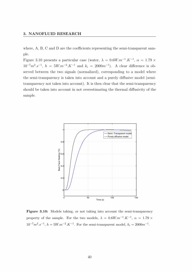
3. NANOFLUID RESEARCH
where, A, B, C and D are the coefficients representing the semi-transparent sam-
ple.
Figure 3.10 presents a particular case (water, λ = 0.6W.m−1.K−1, α = 1.79 ×10⁻⁷m2.s−1, h = 5W.m−2.K−1 and ki = 2000m−1). A clear difference is ob-
served between the two signals (normalized), corresponding to a model where
the semi-transparency is taken into account and a purely diffusive model (semi-
transparency not taken into account). It is then clear that the semi-transparency
should be taken into account in not overestimating the thermal diffusivity of the
sample.
0 50 100 150
0
0.2
0.4
0.6
0.8
1
Time (s)
Ba
ck F
ace H
ea
tin
g (
°C)
Semi−Transparent model
Purely diffusive model
Figure 3.10: Models taking, or not taking into account the semi-transparency
property of the sample. For the two models, λ = 0.6W.m−1.K−1, α = 1.79 ×
10−7m2.s−1, h = 5W.m−2.K−1. For the semi-transparent model, ki = 2000m−1.
40

3.3 Experimental HFE7000-Al2O3 nanofluids
Experimental results
The experimental set-up and thermal model, discussed above, have been
used to determine the thermal diffusivity of three samples. (pure HFE7000, HFE
7000-Al2O3 at 0.5 wt% and 1 wt%). These three fluids were heated for approxi-
mately ten seconds and the temperatures have been normalized. In Figure 3.11,
the experimental signal for HFE 7000-Al2O3 at 0.5 wt% is presented.
−50 0 50 100 150
0
0.2
0.4
0.6
0.8
1
Time (s)
No
rma
lize
d B
ack F
ace
He
atin
g (
°C)
Measurement
Thermal Model
Residuals
Figure 3.11: Comparison of the experimental signal and the developed thermal
model.
For each measurement, the differences between the thermal model and the experi-
mental signal are minimized to estimate the thermal diffusivity, α, the Rosseland’s
coefficient, ki and the heat exchange coefficient, h. The results of these minimiza-
tions are presented in Table 3.5.
41
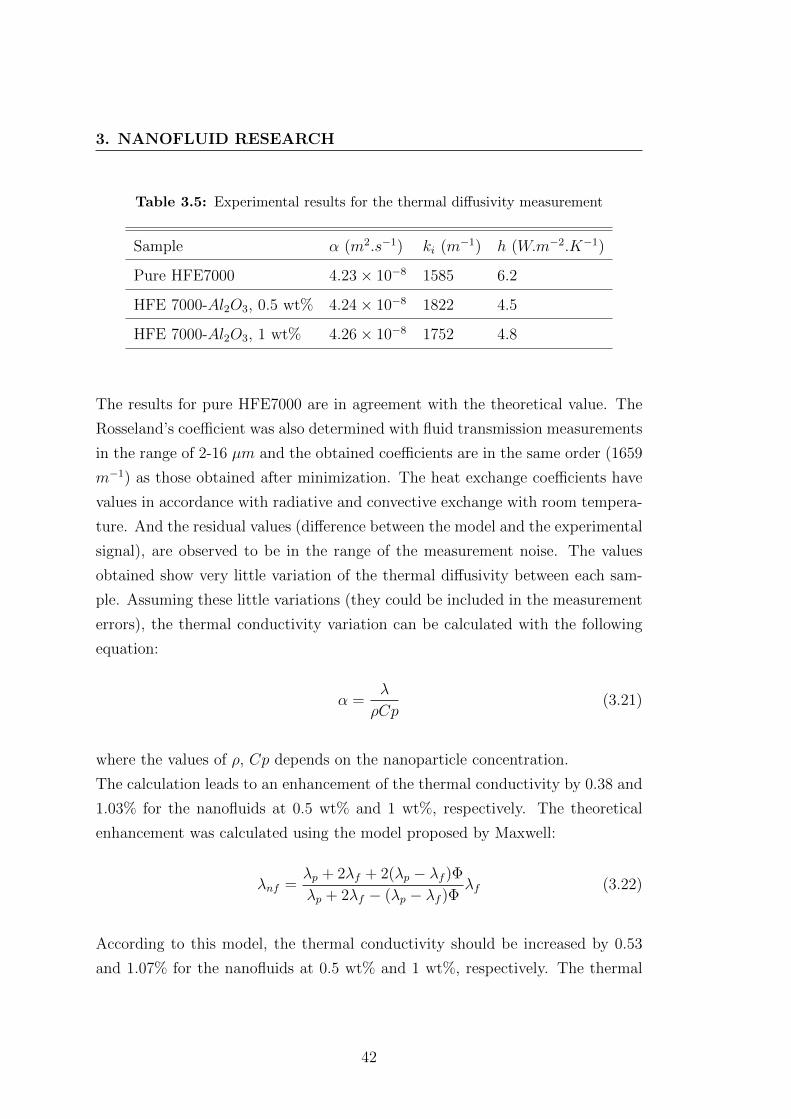
3. NANOFLUID RESEARCH
Table 3.5: Experimental results for the thermal diffusivity measurement
Sample α (m2.s−1) ki (m−1) h (W.m−2.K−1)
Pure HFE7000 4.23× 10⁻⁸ 1585 6.2
HFE 7000-Al2O3, 0.5 wt% 4.24× 10⁻⁸ 1822 4.5
HFE 7000-Al2O3, 1 wt% 4.26× 10⁻⁸ 1752 4.8
The results for pure HFE7000 are in agreement with the theoretical value. The
Rosseland’s coefficient was also determined with fluid transmission measurements
in the range of 2-16 µm and the obtained coefficients are in the same order (1659
m−1) as those obtained after minimization. The heat exchange coefficients have
values in accordance with radiative and convective exchange with room tempera-
ture. And the residual values (difference between the model and the experimental
signal), are observed to be in the range of the measurement noise. The values
obtained show very little variation of the thermal diffusivity between each sam-
ple. Assuming these little variations (they could be included in the measurement
errors), the thermal conductivity variation can be calculated with the following
equation:
α =λ
ρCp(3.21)
where the values of ρ, Cp depends on the nanoparticle concentration.
The calculation leads to an enhancement of the thermal conductivity by 0.38 and
1.03% for the nanofluids at 0.5 wt% and 1 wt%, respectively. The theoretical
enhancement was calculated using the model proposed by Maxwell:
λnf =λp + 2λf + 2(λp − λf )Φλp + 2λf − (λp − λf )Φ
λf (3.22)
According to this model, the thermal conductivity should be increased by 0.53
and 1.07% for the nanofluids at 0.5 wt% and 1 wt%, respectively. The thermal
42
3.4 Conclusions
conductivity determined experimentally is in accordance with the theoretical val-
ues. For low concentrations, the thermal conductivity is slightly increasing with
the increase in particle load. Compared to some results in the literature, where
drastic enhancement in the thermal conductivity was observed, the results are
showing a normal increase in the thermal conductivity, regarding the nanoparti-
cle concentration.
3.4 Conclusions
This chapter introduced the concept of nanofluids and their applications. It ex-
amined the current methods for the preparation and stabilization of such fluids.
The experimental task associated with this chapter was the preparation and char-
acterization of a new heat transfer efficient fluid. While most of the prepared
nanofluids are water, ethylene glycol or ethanol based, no nanofluids presented
in the literature have been made of technical base fluid. HFE7000, from the 3M
company, is used as a coolant, and general low temperature heat transfer appli-
cations. It has been studied by many heat and mass transfer research teams.
HFE7000 based nanofluids were made using the two-step method. Nanoparti-
cles of aluminum oxide were dispersed into the base fluid. It was observed that
the nanofluids prepared at different concentrations remained stable for several
months. Finally, the thermo-physical properties of this novel nanofluid were
characterized, showing very few differences compared to the base fluid. This was
expected in regards with the low load of particles in the prepared nanofluids.
A method to determine the thermal conductivity was developed. It is based on
the measurement of the thermal diffusivity of a sample , but the calculation model
was improved by taking into account the property of semi-transparency in the
infrared wavelengths.
The effectiveness of this nanofluid for heat transfer applications and more pre-
cisely for boiling applications is discussed in the following chapters of this thesis.
43

3. NANOFLUID RESEARCH
44
4
Boiling: General principles
4.1 Introduction
Boiling heat transfer is a very efficient mode of heat transfer due to the latent
heat transferred during the change of phase from a liquid to a gas. In 2002, Zhang
et al. suggested that implementing conventional two-phase systems could offer an
order of magnitude reduction in heat-load-to-weight ratio, as compared to their
single-phase predecessors (39). Boiling heat transfer is defined as a mode of heat
transfer that occurs with a phase change from liquid to vapour. The phenomena
of boiling is classified as pool boiling or flow boiling, depending on the presence
of bulk fluid motion. Boiling is called pool boiling in the absence of fluid flow and
flow boiling (or forced convection boiling) in the presence of flow. In pool boiling
the fluid body is stationary, and any motion of the fluid is due to natural convec-
tion. In flow boiling, the fluid is forced to move by external means, such as pumps.
4.2 The boiling phenomena: general description
The following paragraphs describe the boiling phenomena from an engineering
point of view. It defines the different modes of boiling and presents models and
correlations for practical applications.
45
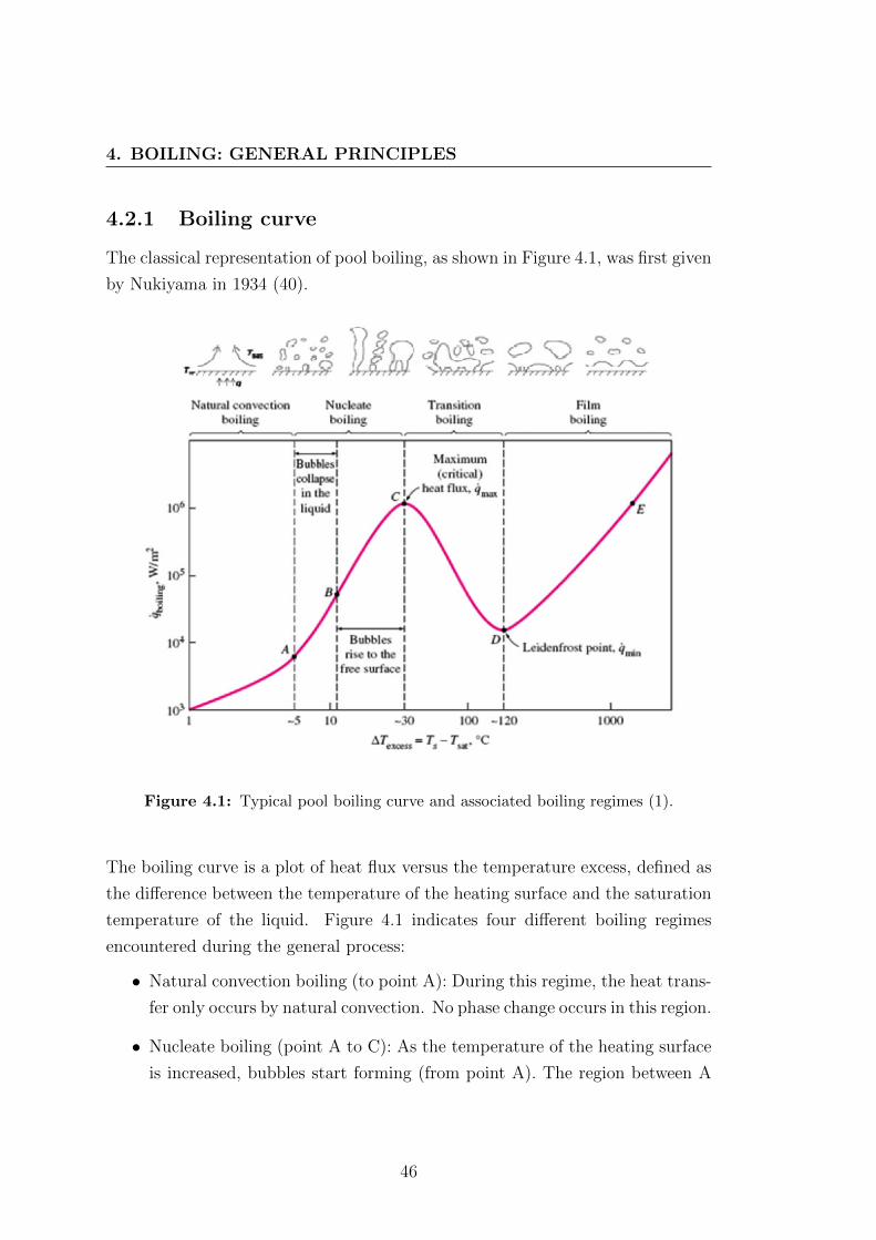
4. BOILING: GENERAL PRINCIPLES
4.2.1 Boiling curve
The classical representation of pool boiling, as shown in Figure 4.1, was first given
by Nukiyama in 1934 (40).
Figure 4.1: Typical pool boiling curve and associated boiling regimes (1).
The boiling curve is a plot of heat flux versus the temperature excess, defined as
the difference between the temperature of the heating surface and the saturation
temperature of the liquid. Figure 4.1 indicates four different boiling regimes
encountered during the general process:
• Natural convection boiling (to point A): During this regime, the heat trans-
fer only occurs by natural convection. No phase change occurs in this region.
• Nucleate boiling (point A to C): As the temperature of the heating surface
is increased, bubbles start forming (from point A). The region between A
46
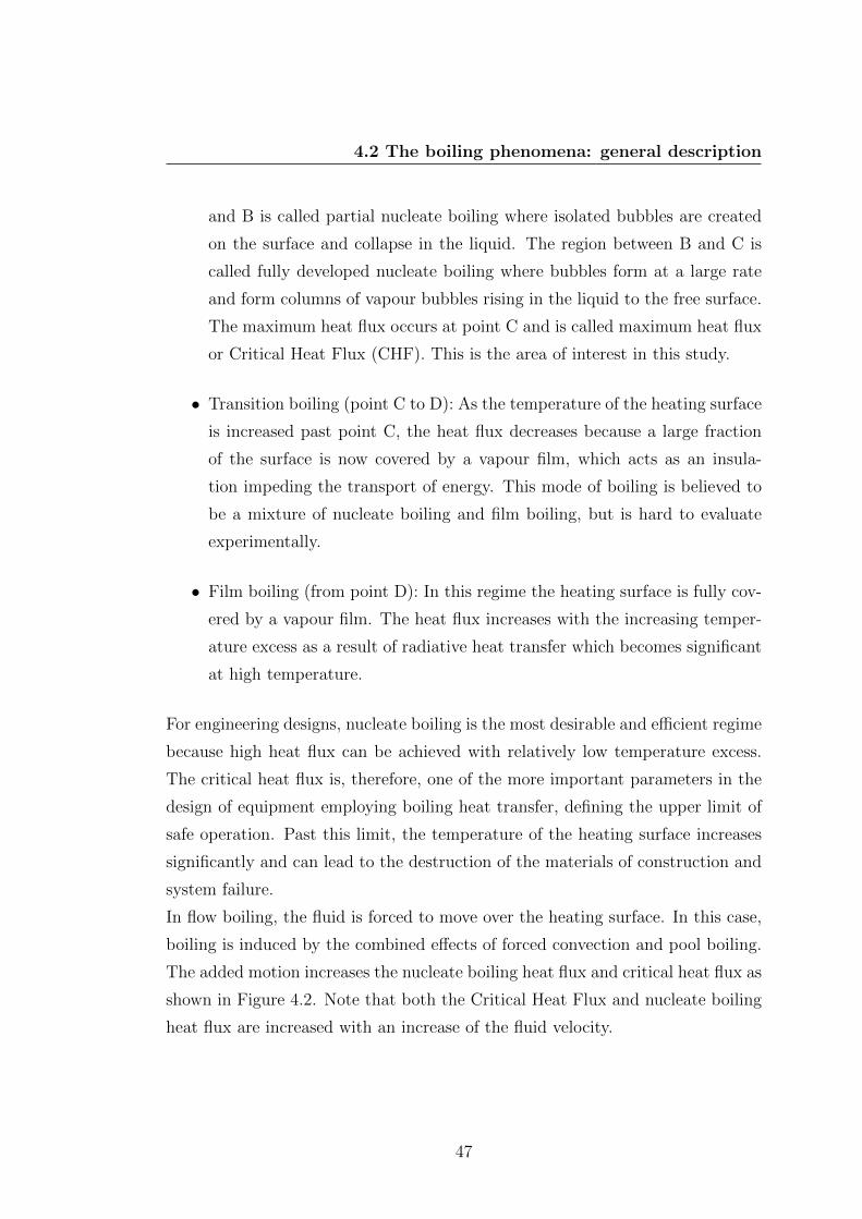
4.2 The boiling phenomena: general description
and B is called partial nucleate boiling where isolated bubbles are created
on the surface and collapse in the liquid. The region between B and C is
called fully developed nucleate boiling where bubbles form at a large rate
and form columns of vapour bubbles rising in the liquid to the free surface.
The maximum heat flux occurs at point C and is called maximum heat flux
or Critical Heat Flux (CHF). This is the area of interest in this study.
• Transition boiling (point C to D): As the temperature of the heating surface
is increased past point C, the heat flux decreases because a large fraction
of the surface is now covered by a vapour film, which acts as an insula-
tion impeding the transport of energy. This mode of boiling is believed to
be a mixture of nucleate boiling and film boiling, but is hard to evaluate
experimentally.
• Film boiling (from point D): In this regime the heating surface is fully cov-
ered by a vapour film. The heat flux increases with the increasing temper-
ature excess as a result of radiative heat transfer which becomes significant
at high temperature.
For engineering designs, nucleate boiling is the most desirable and efficient regime
because high heat flux can be achieved with relatively low temperature excess.
The critical heat flux is, therefore, one of the more important parameters in the
design of equipment employing boiling heat transfer, defining the upper limit of
safe operation. Past this limit, the temperature of the heating surface increases
significantly and can lead to the destruction of the materials of construction and
system failure.
In flow boiling, the fluid is forced to move over the heating surface. In this case,
boiling is induced by the combined effects of forced convection and pool boiling.
The added motion increases the nucleate boiling heat flux and critical heat flux as
shown in Figure 4.2. Note that both the Critical Heat Flux and nucleate boiling
heat flux are increased with an increase of the fluid velocity.
47
4. BOILING: GENERAL PRINCIPLES
Figure 4.2: Typical flow boiling curve at different fluid velocities (1).
4.2.2 Heat and mass transfer correlations
From all the regimes describing the boiling curve, the nucleate boiling regime
is the most desirable regime for practical applications due to its high efficiency.
High heat transfer coefficients can be obtained for relatively low wall superheats.
The region between the beginning of the nucleate boiling regime to the critical
heat flux is of great interest for the design of industrial systems and calls for a
better understanding of the mechanism involved in the process. The following
sections are dedicated to describing the main efforts on the description and mod-
elisation of the nucleate boiling heat transfer and the critical heat flux prediction.
48
4.2 The boiling phenomena: general description
4.2.2.1 Nucleate boiling
The importance of nucleate boiling in a wide range of application makes it an
important research subject. In this section, some heat transfer models and cor-
relations describing the nucleate boiling phenomena are proposed. Boiling heat
transfer is a complex phenomena where several parameters are involved, and
treated differently by researchers.
The first approach, proposed by Rohsenow, makes an analogy between the heat
exchanges in forced convection and those associated with nucleate boiling in a
pool. In this case, it is proposed that the heat transfers follow a model based on
(41):
Nub =hLbλt
= ARe1−rPr1−s (4.1)
where h is he heat transfer coefficient defined by: h = qTw−Tsat , Lb is a character-
istic length of the vapour bubble, Re is the Reynolds number defined by:
Re =ρvUbLbµl
(4.2)
where Ub is the characteristic velocity of the bubble. Rohsenow’s model is making
several assumptions:
The characteristic length is the detachment diameter of the bubble and is (42):
Lb = Db = Cbθ
[2σ
g(ρl − ρv)
] 12
(4.3)
The velocity of the bubble is the velocity of the vapour surface:
Ub =q
ρvhlv(4.4)
and the heat transfer coefficient is defined as:
49

4. BOILING: GENERAL PRINCIPLES
h =q
Tw − Tsat(4.5)
Expending equation 4.1 with the relationships seen in equations 4.2-4.5, we obtain
Rohsenow’s model:
q
µlhlv
(σ
g(ρl − ρv)
) 12
=
(1
Csf
) 1r
Pr−sr
(Cpl(Tp − Tsat)
Llv
) 1r
(4.6)
where the values of r and s are 0.33 and 1.7, respectively. For water, s equals
1. Csf is an empirical parameter that depends on the liquid-material and is
expressed as:
Csf =
√2Cbθ
A(4.7)
The values of Csf vary depending on the liquid and material. For example for
water-copper, Csf is equal 0.012 and is 0.006 for water-nickel. In general, the
equation proposed by Rohsenhow is not very precise but gives a good first ap-
proximation of the heat flux. This is explained by the fact that the model was
developed in forced convection and subcooled conditions while the values of r,s
and Csf were determined in pool boiling conditions.
Among the most commonly used correlations, is the one proposed by Forster
and Zuber (43). In their work, they based the model on the micro convection in
the layer close to the wall in subcooled cases and using dynamical and geometrical
characteristics of the bubbles. The proposed model is as follows:
q = 0.0015.
(ρlπ((Tw − Tsat)λl)2
µlαl(ρv.hlv)2
)5/8
.
(Cplµlλl
)1/3
.
(ρlR
3eq
2σ
)−1/4
.
√αlπ.ρv.hlv
(4.8)
50

4.2 The boiling phenomena: general description
where Re is the equilibrium radius of a vapour bubble defined as:
Req =2σ
ρl(Tw − Tsat).RT 2
sat
Mhlv=
2σ
hlv(Tw − Tsat).Tsatρv
(4.9)
where R is the universal gas constant and M is the molar mass of the liquid.
The correlation presented is adimensional and is not as known as the dimensional
equation of the correlation expressed as follows:
q = 0.00122.λ0.79l C0.45
pl ρ0.49l
σ0.5µ0.29l h0.24
lv ρ0.24v
.(Tw − Tsat)1.24.∆p0.75sat (4.10)
∆psat represents the saturation pressure difference corresponding to the super-
heat Tw−Tsat. One of the disadvantages of the correlation is the fact that it only
takes into account the physical and thermal properties of the liquid. In order to
have more accurate results, the surface characteristics should also be taken into
account, as done by Rohsenow in equation 4.6.
Mikic and Roshenow later proposed a model taking into account the effect of
the heating surface for saturation conditions (44). The concept used is based on
the exchange between the liquid and the vapour, developed for subcooled boiling
conditions, and extended for saturated boiling conditions. They proposed that
the total heat flux depends on the heat flux related to the vapour bubbles and
partially due to the convection where the bubbles have no influence. The previ-
ous model from Rohsenow was only taking into account the convection due to the
vapour bubble rise and is then completed by taking into account the effects of the
bubbles. It is considered that the surface occupied by the bubble received liquid
at the saturation temperature when the bubble departed from its nucleation site,
and is then heated by conduction. The fluid layer overheated is replaced at the
same frequency as the bubble detachment frequency. The equation to determine
the heat flux due to the bubbles then depends on the departure frequency f , the
detachment diameter Dd, the nucleation site density Nb and the fluid properties:
qb = 2NbD2b (Tw − Tsat)
√π(λρCp)lf (4.11)
51
4. BOILING: GENERAL PRINCIPLES
To obtain the total heat flux, the heat flux due to natural convection has to
be added, and this is calculated with the well-known single phase convection
correlation.
q = qconv.
(1−NbK
(πD2
b
4
))+ qb (4.12)
where K is a constant.
The determination of the nucleation site density can be estimated, according to
Mikic and Rohsenhow, by comparing the maximum and minimum sizes of the
active nucleation sites:
Nb =
(Rc,max
Rc,min
)m(4.13)
Cooper also proposed a correlation depending on the characteristics of the sur-
face (45). His model was developed based on the reduced pressure p+, the surface
roughness Ra and the molar mass M of the fluid.
h = 55p+A.(−0.4343.lnp+)−0.55.M−0.5.q0.67 (4.14)
where A = 0.12− 0.4343.lnRa and p+ = P/Pc.
The surface roughness can be related to the number of active nucleation sites,
and as a result, as the surface roughness increases, the heat transferred increases.
This correlation is able to cover a wide range of reduced pressure and can be
adapted to different heating surfaces.
In order to obtain correlations for a wide range of applications, Stephan and
Abdelsalam used a simplified method (46). They applied a regression analysis
to almost 5000 existing experimental data points for natural convection boiling
heat transfer. The resulting corrections were categorized in four groups: water,
hydrocarbons, cryogenic fluids and refrigerants. They used different sets of di-
mensionless numbers for each group (some dimensionless numbers are important
for one group but irrelevant for others):
52
4.2 The boiling phenomena: general description
• Water
Nu = 2.46 ∗ 106.X0.6731 .X−1.58
4 .X1.263 .X5.22
8 (4.15)
for 10−4 < p+ < 0.886 and θ = 45
• Hydrocarbons
Nu = 0.0546.(X0.55 .X1)0.67.X4.33
8 .X0.2484 (4.16)
for 5, 7 ∗ 10−3 < p+ < 0.9 and θ = 35
• Cryogenic fluid
Nu = 4.82X0.6241 .X0.117
7 .X0.2575 .X0.374
3 .X−0.3294 (4.17)
for 4 ∗ 10−3 < p+ < 0.97 and θ = 1
• Refrigerant
Nu = 207X0.7451 .X0.581
5 .X0.5336 (4.18)
for 3 ∗ 10−3 < p+ < 0.78 and θ = 35
The values of the contact angle θ were assumed from the literature since none of
the experiments simultaneously measured the heat transfer coefficient and con-
tact angle of the vapour bubbles.
The dimensionless numbers appearing in these different correlations are:
Nu = q.D∆Tλl
, X1 = q.DTsatλl
, X2 =α2l ρlσD
X3 =CplTsatD
2
α2l
, X4 = hlvD2
λ2l, X5 = ρv
ρl
X6 = µlαl
, X7 = (ρCpλ)w(ρCpλ)l
, X8 = ρl−ρvρl
The authors also proposed that a correlation could be valid for all the substances,
but recommends not to use it since the accuracy would be less than each individ-
ual equation or would add too much complexity.
53
4. BOILING: GENERAL PRINCIPLES
Other models and correlations have been proposed. They are based on differ-
ent concepts or assumptions. The equations based on micro convection models
and vapour-liquid exchange models, which are the most commonly used are pre-
sented herein. Numerous other concepts were used to model the heat transfer
coefficient during nucleate pool boiling such as an analogy with natural convec-
tion heat transfer, models based on latent heat and micro layer evaporation effect
or formulations based on thermodynamic similitude.
4.2.2.2 Critical heat flux
As shown in Figure 4.1, the pool boiling curve exhibits a maximum, called the
Critical Heat Flux (referred as CHF), at the transition between nucleate and
transition boiling. It corresponds to the maximum heat flux that can be removed
from the heated surface. When the heating is performed with a set heat flux, a
sharp increase of the surface temperature above the critical heat flux is obtained,
which can lead to the burnout of the heating surface and damage the system. If
experiments are performed with a set temperature, the critical heat flux corre-
sponds to a decrease of the heat flux transmitted from the heating surface to the
fluid due to the vapour accumulation on the wall, forming a thermal insulation.
In the same manner as for the nucleate boiling modelisation, several theories have
been proposed to describe the mechanism leading to the the critical heat flux.
These theories can usually be categorized in four groups of mechanism:
• The hydrodynamic instability theory: due to liquid-vapour instability, the
liquid can not recover the heating surface and a vapour layer is created.
• The macro layer dryout theory: it supposes the existence of a liquid layer
under the vapour bubble, causing its departure from the surface. If this
layer evaporates completely we reach the critical heat flux.
• The hot/dry spot theory: very hot spots are created on the surface; due to
the very high temperature the wetting of the heating surface is no longer
possible.
54
4.2 The boiling phenomena: general description
• The bubble interaction theory: due to the increase of the nucleation site
density, the vapour bubbles merge and prevent the liquid from recovering
the heating surface by creating a vapour layer on the surface.
Kutateladze then Zuber were the first to propose a model predicting the critical
heat flux (47). They assumed that the critical heat flux occurrence is dominated
by hydrodynamic forces and is attained when the vapour columns leaving the
surface are becoming Helmholtz unstable (unstable growth of perturbations in
the vapour columns leaving the surface). As the vapour rising is unstable, it
appears as waves at the liquid-vapour interface (Taylor instability), breaking the
interface in different positions from where vapour columns are forming (spaced
by a wavelength λRT ).
The critical heat flux is evaluated based on the energy balance:
qCHF = ρvhlvjv (4.19)
where, jv is the superficial vapour velocity expressed as:
jv =
√2πσ
ρvλRT(4.20)
and the Rayleigh-Taylor instability wavelength, λRT is:
λRT =
[σ
g(ρlk − ρv)
]1/2
(4.21)
By combining equation 4.19-4.21, the expression of the critical heat flux given by
Zuber is obtained as:
qCHF =π
24ρvhlv
[σg(ρl − ρv)
ρ2v
]1/4
(4.22)
It is interesting to note that the model presented here only takes into account the
thermophysical properties of the fluid and gravity and does not account for the
heating surface characteristics. Also, this model was proposed for a horizontal
55
4. BOILING: GENERAL PRINCIPLES
infinite plate under saturated conditions.
Lienhard and Dhir extended the theory for several geometries (48). They re-
lated the critical heat flux for a specific geometry to the CHF proposed by Zuber
(infinite horizontal plate) with a function of a characteristics length L′:
qCHF =π
24f(L′)ρvhlv
[σg(ρl − ρv)
ρ2v
]1/4
(4.23)
L′ = L
√g(ρl − ρv)
σ(4.24)
The explanation of the CHF with the macro layer theory is based on the as-
sumption that a large vapour bubble is produced by many other small bubbles,
however above the heating surface. These large vapour bubbles are separated
from the surface by a liquid layer (macro layer). It is hypothesized that the criti-
cal heat flux is attained when the macro layer dries out, as explained by Haramura
and Katto, who developed the following model based on these assumptions and
related to Zuber’s model (49):
qCHF =qCHF,z0.131
.
(π4
21132
)1/16
.
(AvAw
)5/8
.
(1− Av
Aw
)5/16
.
(ρlρv
+ 1
( 11ρl16ρv
)3/5
)5/16
(4.25)
where, qCHF,z is the critical heat flux defined by Zuber and AvAw
represents the
transversal surface of the vapour columns over the total wall surface and expressed
as:AvAw
= 0.0584
(ρvρl
)1/5
(4.26)
The critical heat flux also only depends on the fluid properties, without taking
into account the surface characteristics. Even if in this model the macro layer
is assumed to be very thin, experimental visualization has shown that the layer
56
4.2 The boiling phenomena: general description
is constantly renewed. This is raising some doubts on the validity of the model
although the experimental values found for water and the refrigerants show good
agreement with the model.
In order to account for the surface characteristics, Kandlikar developed a model
incorporating the surface orientation, the contact angle at the liquid-surface in-
terface, and the liquid subcooling level (50):
qCHF = hlvρ1/2v
(1 + cosθ
16
)[2
π+π
4(1 + cosθ)cosβ
]1/2
[σg(ρl − ρv)]1/4 (4.27)
where, θ is the receding contact angle and β is the surface orientation. The
model was shown to be valid for flat surfaces with orientation between β = 0
and β = 90. (horizontal and vertical orientation). According to the model, the
CHF decreases with the increase of contact angle and orientation.
This model is also used by Kandlikar to incorporate the effect of the liquid sub-
cooling level on the critical heat flux and is expressed as:
qCHF,sub = qCHF,sat
(1 +
Tsat − TsubTw − Tsat
)(4.28)
where, qCHF,sub and qCHF,sat are the CHF under subcooled and saturated condi-
tions, respectively. It shows that the critical heat flux under subcooled conditions
is greater than in saturated conditions. This is explained by the additional heat
transferred to the subcooled fluid.
57
4. BOILING: GENERAL PRINCIPLES
4.3 Boiling of nanofluids
Research into the possible enhancement and the parameters governing boiling is
ongoing with some current research conducted on nanofluid heat transfer, the
Heat Transfer Coefficients (HTC), and the Critical Heat Flux (CHF) during the
nucleate boiling regime. Although this research is important, the vast majority
of nanofluid boiling studies have, and even now remain, focused on pool boiling
rather than the more practical flow boiling.
4.3.1 Pool boiling
Nanofluid boiling has shown promise for at least 25 years when Yang and Maa first
demonstrated that nanoparticles of alumina (50, 300, 1000 nm) in water, with
concentrations of 0.1 and 0.5 wt% (particle mass concentration of the nanofluid),
can significantly lower the superheat needed for a given flux (51). They showed
that the greatest improvement was for the smallest particles at the lowest con-
centration, while at 0.5 wt% all particle sizes performed equally. However, the
results concerning nanofluid pool boiling remain inconsistent. For the nucleate
boiling heat transfer coefficient, some studies reported no change, enhancement
or deterioration compared to the initial base fluid as discussed below.
Vassalo et al. studied pool boiling with 15 and 50 nm silica particles in water
with concentration of 0.5 vol.% (52). The nucleate boiling regime was shown
to be unaffected but all suspensions were observed to increase the Critical Heat
Flux by ≈60%. You et al. showed very little or no changes in the HTC (53).
These experiments were conducted with Al2O3 nanoparticles at a low pressure
and mostly focused on the CHF. Bubble departure from the heated surface was
decreased but bubble size was increased, giving little overall net change in the
nucleate boiling regime.
Das et al. worked with alumina-water nanofluids and concentrations of 0.1 to 4
vol. % (2). It was found, as shown in Figure 4.3 that the nucleate boiling curve
shifted to higher temperatures as the nanoparticle concentration was increased.
Furthermore, a higher wall temperature for the same heat flux was achieved,
which corresponds to a degradation in the heat transfer phenomenon.
58
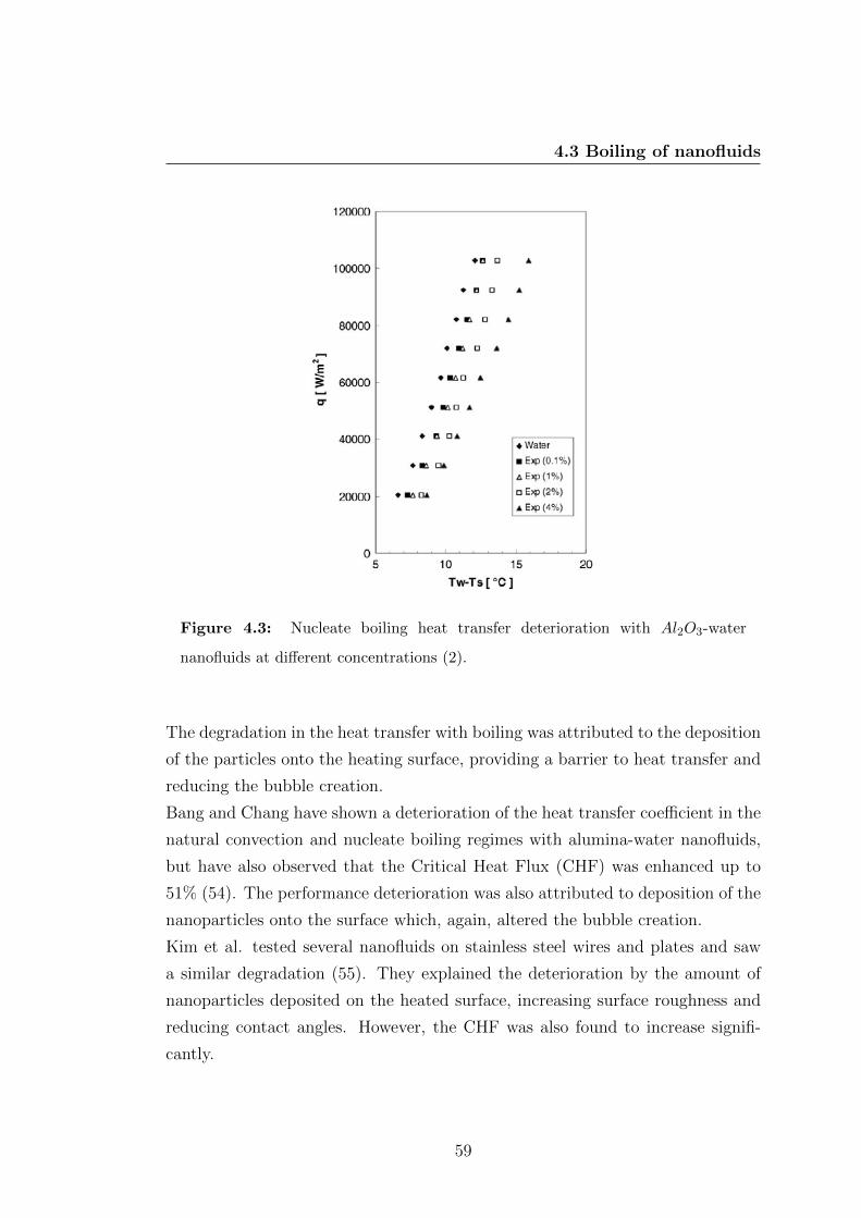
4.3 Boiling of nanofluids
Figure 4.3: Nucleate boiling heat transfer deterioration with Al2O3-water
nanofluids at different concentrations (2).
The degradation in the heat transfer with boiling was attributed to the deposition
of the particles onto the heating surface, providing a barrier to heat transfer and
reducing the bubble creation.
Bang and Chang have shown a deterioration of the heat transfer coefficient in the
natural convection and nucleate boiling regimes with alumina-water nanofluids,
but have also observed that the Critical Heat Flux (CHF) was enhanced up to
51% (54). The performance deterioration was also attributed to deposition of the
nanoparticles onto the surface which, again, altered the bubble creation.
Kim et al. tested several nanofluids on stainless steel wires and plates and saw
a similar degradation (55). They explained the deterioration by the amount of
nanoparticles deposited on the heated surface, increasing surface roughness and
reducing contact angles. However, the CHF was also found to increase signifi-
cantly.
59

4. BOILING: GENERAL PRINCIPLES
Wen and Ding contradicted these results when they observed up to 40% en-
hancement in nucleate boiling also using alumina-water nanofluids (56). It was
thought that this enhancement was due to the stability of the nanofluids, which
apparently did not deposit on the surface. Shi et al. conducted experiments with
iron and alumina nanofluids boiling on a copper block (57). They concluded that
Fe nanoparticles showed higher enhancement than Al2O3 nanoparticles and that
these ameliorations were due to higher thermal conductivities and lowered surface
tension.
Soltani et al. performed pool boiling experiments using Al2O3-water and SnO2-
water nanofluids (3). A 2% concentration of particles enhanced the nucleate
boiling by 20% for the Tin oxide-water nanofluid and by 30% for the alumina-
water nanofluid, as shown in Figure 4.4.
Figure 4.4: Nucleate boiling heat transfers enhancement with Al2O3-water
nanofluid at different concentrations (3).
This enhancement was again explained by the good stability of the nanofluids and
the significant increase of the thermal conductivities of the nanofluids. To sum-
marize, this published work exhibited improvements and enhancements, ranging
60
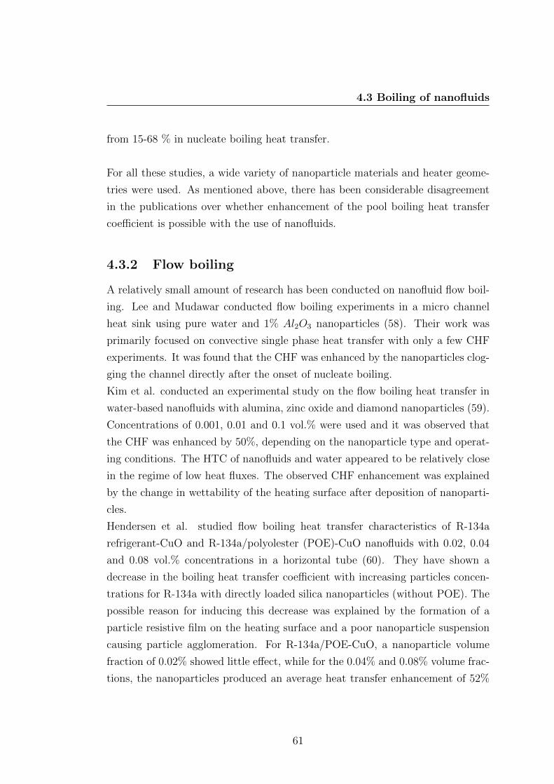
4.3 Boiling of nanofluids
from 15-68 % in nucleate boiling heat transfer.
For all these studies, a wide variety of nanoparticle materials and heater geome-
tries were used. As mentioned above, there has been considerable disagreement
in the publications over whether enhancement of the pool boiling heat transfer
coefficient is possible with the use of nanofluids.
4.3.2 Flow boiling
A relatively small amount of research has been conducted on nanofluid flow boil-
ing. Lee and Mudawar conducted flow boiling experiments in a micro channel
heat sink using pure water and 1% Al2O3 nanoparticles (58). Their work was
primarily focused on convective single phase heat transfer with only a few CHF
experiments. It was found that the CHF was enhanced by the nanoparticles clog-
ging the channel directly after the onset of nucleate boiling.
Kim et al. conducted an experimental study on the flow boiling heat transfer in
water-based nanofluids with alumina, zinc oxide and diamond nanoparticles (59).
Concentrations of 0.001, 0.01 and 0.1 vol.% were used and it was observed that
the CHF was enhanced by 50%, depending on the nanoparticle type and operat-
ing conditions. The HTC of nanofluids and water appeared to be relatively close
in the regime of low heat fluxes. The observed CHF enhancement was explained
by the change in wettability of the heating surface after deposition of nanoparti-
cles.
Hendersen et al. studied flow boiling heat transfer characteristics of R-134a
refrigerant-CuO and R-134a/polyolester (POE)-CuO nanofluids with 0.02, 0.04
and 0.08 vol.% concentrations in a horizontal tube (60). They have shown a
decrease in the boiling heat transfer coefficient with increasing particles concen-
trations for R-134a with directly loaded silica nanoparticles (without POE). The
possible reason for inducing this decrease was explained by the formation of a
particle resistive film on the heating surface and a poor nanoparticle suspension
causing particle agglomeration. For R-134a/POE-CuO, a nanoparticle volume
fraction of 0.02% showed little effect, while for the 0.04% and 0.08% volume frac-
tions, the nanoparticles produced an average heat transfer enhancement of 52%
61
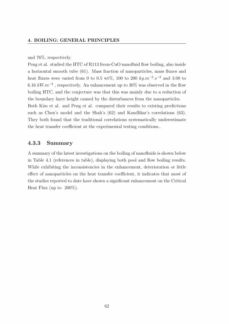
4. BOILING: GENERAL PRINCIPLES
and 76%, respectively.
Peng et al. studied the HTC of R113 freon-CuO nanofluid flow boiling, also inside
a horizontal smooth tube (61). Mass fraction of nanoparticles, mass fluxes and
heat fluxes were varied from 0 to 0.5 wt%, 100 to 200 kg.m−2.s−2 and 3.08 to
6.16 kW.m−2 , respectively. An enhancement up to 30% was observed in the flow
boiling HTC, and the conjecture was that this was mainly due to a reduction of
the boundary layer height caused by the disturbances from the nanoparticles.
Both Kim et al. and Peng et al. compared their results to existing predictions
such as Chen’s model and the Shah’s (62) and Kandlikar’s correlations (63).
They both found that the traditional correlations systematically underestimate
the heat transfer coefficient at the experimental testing conditions..
4.3.3 Summary
A summary of the latest investigations on the boiling of nanofluids is shown below
in Table 4.1 (references in table), displaying both pool and flow boiling results.
While exhibiting the inconsistencies in the enhancement, deterioration or little
effect of nanoparticles on the heat transfer coefficient, it indicates that most of
the studies reported to date have shown a significant enhancement on the Critical
Heat Flux (up to 200%).
62
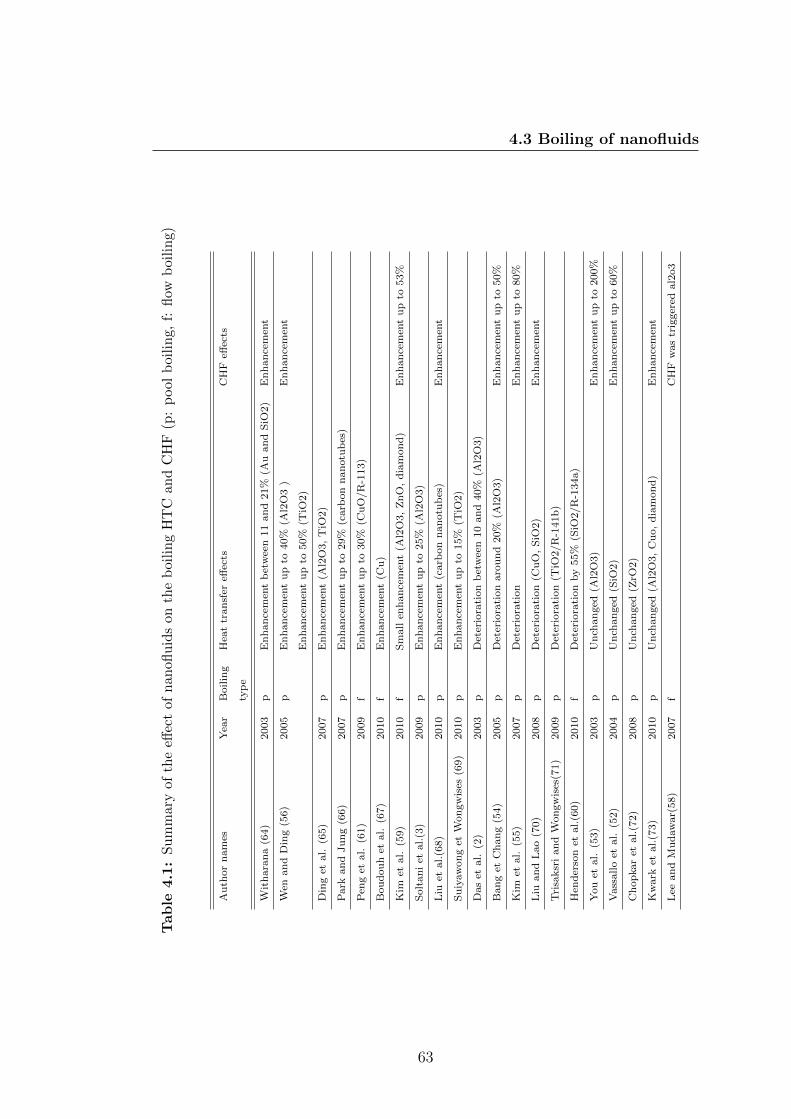
4.3 Boiling of nanofluids
Tab
le4.1
:S
um
mar
yof
the
effec
tof
nan
ofluid
son
the
boi
lin
gH
TC
and
CH
F(p
:p
ool
boil
ing,
f:fl
owb
oil
ing)
Au
thor
nam
esY
ear
Boilin
gH
eat
tran
sfer
effec
tsC
HF
effec
ts
typ
e
Wit
hara
na
(64)
2003
pE
nh
an
cem
ent
bet
wee
n11
an
d21%
(Au
an
dS
iO2)
En
han
cem
ent
Wen
an
dD
ing
(56)
2005
pE
nh
an
cem
ent
up
to40%
(Al2
O3
)E
nh
an
cem
ent
En
han
cem
ent
up
to50%
(TiO
2)
Din
get
al.
(65)
2007
pE
nh
an
cem
ent
(Al2
O3,
TiO
2)
Park
an
dJu
ng
(66)
2007
pE
nh
an
cem
ent
up
to29%
(carb
on
nan
otu
bes
)
Pen
get
al.
(61)
2009
fE
nh
an
cem
ent
up
to30%
(Cu
O/R
-113)
Bou
dou
het
al.
(67)
2010
fE
nh
an
cem
ent
(Cu
)
Kim
etal.
(59)
2010
fS
mall
enh
an
cem
ent
(Al2
O3,
Zn
O,
dia
mon
d)
Enh
an
cem
ent
up
to53%
Solt
an
iet
al.(3
)2009
pE
nh
an
cem
ent
up
to25%
(Al2
O3)
Liu
etal.(6
8)
2010
pE
nh
an
cem
ent
(carb
on
nan
otu
bes
)E
nh
an
cem
ent
Su
iyaw
on
get
Won
gw
ises
(69)
2010
pE
nh
an
cem
ent
up
to15%
(TiO
2)
Das
etal.
(2)
2003
pD
eter
iora
tion
bet
wee
n10
an
d40%
(Al2
O3)
Ban
get
Ch
an
g(5
4)
2005
pD
eter
iora
tion
aro
un
d20%
(Al2
O3)
En
han
cem
ent
up
to50%
Kim
etal.
(55)
2007
pD
eter
iora
tion
En
han
cem
ent
up
to80%
Liu
an
dL
ao
(70)
2008
pD
eter
iora
tion
(Cu
O,
SiO
2)
En
han
cem
ent
Tri
saksr
iand
Won
gw
ises
(71)
2009
pD
eter
iora
tion
(TiO
2/R
-141b
)
Hen
der
son
etal.(6
0)
2010
fD
eter
iora
tion
by
55%
(SiO
2/R
-134a)
You
etal.
(53)
2003
pU
nch
an
ged
(Al2
O3)
En
han
cem
ent
up
to200%
Vass
allo
etal.
(52)
2004
pU
nch
an
ged
(SiO
2)
En
han
cem
ent
up
to60%
Ch
op
kar
etal.(7
2)
2008
pU
nch
an
ged
(ZrO
2)
Kw
ark
etal.(7
3)
2010
pU
nch
an
ged
(Al2
O3,
Cu
o,
dia
mon
d)
En
han
cem
ent
Lee
an
dM
ud
aw
ar(
58)
2007
fC
HF
was
trig
ger
edal2
o3
63
4. BOILING: GENERAL PRINCIPLES
4.4 Experimental set-up: Pool boiling
Heat transfer and critical heat flux measurement were undertaken in the schematic
of the experimental apparatus shown in Figure 4.5. This consists of a wire heater
horizontally submerged in the fluid to be tested. The fluid is enclosed in a glass
cylinder with a 10 cm diameter, at atmospheric pressure. A reflux is mounted on
top of the cylinder where the vapour will be condensed, maintaining a constant
pressure inside the chamber. Boiling occurs on the horizontal thin platinum wire
that is heated. The platinum wire (Goodfellow, 99.9% purity) of diameter 50
µm and 35 mm length is submerged at a depth of 50mm below the free surface.
Platinum wire was selected, since this wire can be used both as heater and tem-
perature sensor. Platinum low thermal capacity gives the wire the advantage of
being very sensitive to heat flux and temperature changes. The end of the plat-
inum wire was soldered onto a much larger copper wire to ensure a low resistance
path for the electric current . The wire temperature was determined from mea-
surements of the electrical resistance by using the known resistivity-temperature
curve for platinum.
The boiling process was induced by a current passing through the wire, leading
to heat production by the Joule effect. The power supply consisted of an ISO-
TECH IPS-405 stabilized power supply, delivering up to 40V and 5A and allowing
studies at constant voltage or current. A K-type thermocouple placed far from
the heating wire was used to permanently acquire the bulk fluid temperature.
All the pieces of experimental apparatus were enclosed in closed box where the
temperature was controlled via PID and Peltier elements.
Before any experiments could be performed, dissolved gases needed to be removed
from the fluid. The fluid was heated near its saturation temperature and boiled
for several minutes. The gases were discharged and the fluid was left to cool
down.
The experimental procedure was as follows. The closed box and the test fluid
were preheated to the desired temperature, then the wire was heated little by lit-
tle at low heat flux in order to remove any gas bubbles sticking on the platinum
wire.
The experiment was started by increasing the power supplied to the wire in small
64
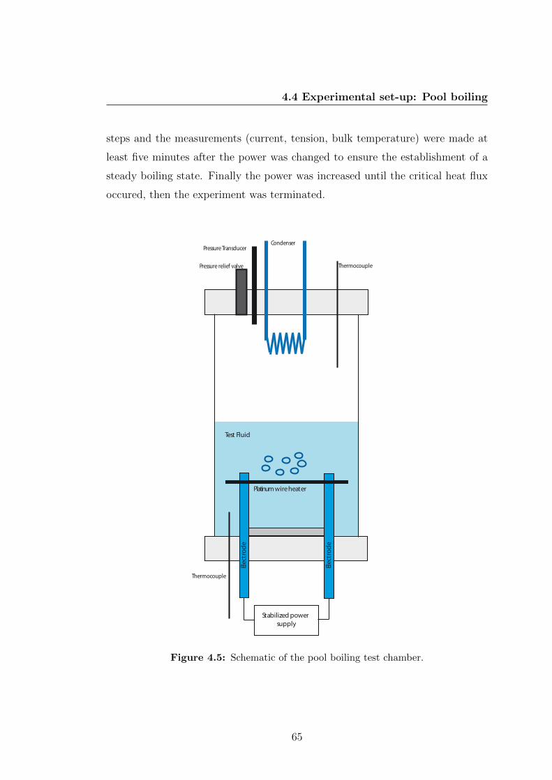
4.4 Experimental set-up: Pool boiling
steps and the measurements (current, tension, bulk temperature) were made at
least five minutes after the power was changed to ensure the establishment of a
steady boiling state. Finally the power was increased until the critical heat flux
occured, then the experiment was terminated.
Thermocouple
Thermocouple
Condenser
Pressure relief valve
Pressure TransducerEle
ctro
de
Elect
rode
Platinum wire heater
Test Fluid
Stabilized powersupply
Figure 4.5: Schematic of the pool boiling test chamber.
65

4. BOILING: GENERAL PRINCIPLES
The heat flux , q, at the heated surface was calculated from the power supplied
to the platinum wire and the heated area (the total surface of the wire). As the
wire was very thin (50µm), it was assumed that the temperature was radially ho-
mogeneous and along the surface. The power delivered to the wire is calculated
from the applied voltage, and measured current from equation 4.29:
q =UI
A=
UI
πDL(4.29)
where, U and I are the input voltage and current, and D and L are the wire
diameter and length, respectively.
The superheat temperature ∆T , is the difference between the surface temperature
of the wire, or wall temperature Tw, and the saturation temperature, Tsat of the
tested fluid:
∆T = Tw − Tsat (4.30)
The determination of the wall temperature is made through the measurement
of the resistance of the wire. Platinum wire has the advantage of being used as
heating surface and thermometer at the same time. The relationship between a
platinum wire and its temperature is given by equation 4.31.
R(T ) = R0(1 + AT +BT 2 + C(T − 100)T 3) (4.31)
In the above equation, R(T ) and R0 are the resistance of the wire at the deter-
mined temperature and resistance at 0K, respectively. The values of A, B and C
are found in the literature to be:
A = 3.85× 10⁻³K−1
B = 5.775× 10⁻⁷K−2
C = 4.183× 10⁻¹²K−4 if T < 100K and 0 if T > 100K
Since HFE7000 is a low boiling temperature fluid, the temperature reached in
the experiment is relatively low. The relationship between the wall temperature
66

4.4 Experimental set-up: Pool boiling
and the wire resistance can be simplified.
The resistance of the platinum at 0K being unknown, the calculation of the wall
temperature is done as follows:
R(Ti) = R0(1 + ATi) (4.32)
R(Tw) = R0(1 + ATw) (4.33)
Tw =Rw
Ri
(1 + ATi)− 1 (4.34)
where R0, R(Ti) and Rw are the resistance of the of the wire at 0K, at the ini-
tial bulk fluid temperature and the measured resistance during the experiment,
respectively. Ti is the initial temperature of the bulk fluid.
Finally, the heat transfer coefficient associated with the boiling process is calcu-
lated from equation 4.35.
h =q
(Tw − Tsat)(4.35)
The sum of squares method was used to quantify the measurement uncertainties of
the heat flux, superheat and heat transfer coefficient. The uncertainty associated
with the heat flux can be determined as :
δq =
√(δUUq
)2
+
(δIIq
)2
+
(δSSq
)2
(4.36)
where, δU , δI and δS are the uncertainties of the voltage, current and surface area,
respectively. The measurement error associated with the voltage is ±10mV . The
current measurement error is ±2mA. The length of the wire is 38mm ± 0.1mm
and the diameter is 50µm±1%. Using the previous equation, the maximum heat
flux uncertainty calculated was approximately 4%.
In the same manner, the uncertainty of the wall superheat is calculated as :
δTw =
√(δRwRw
Tw
)2
+
(δRTiRT i
Tw
)2
+
(δTiTiTw
)2
(4.37)
67
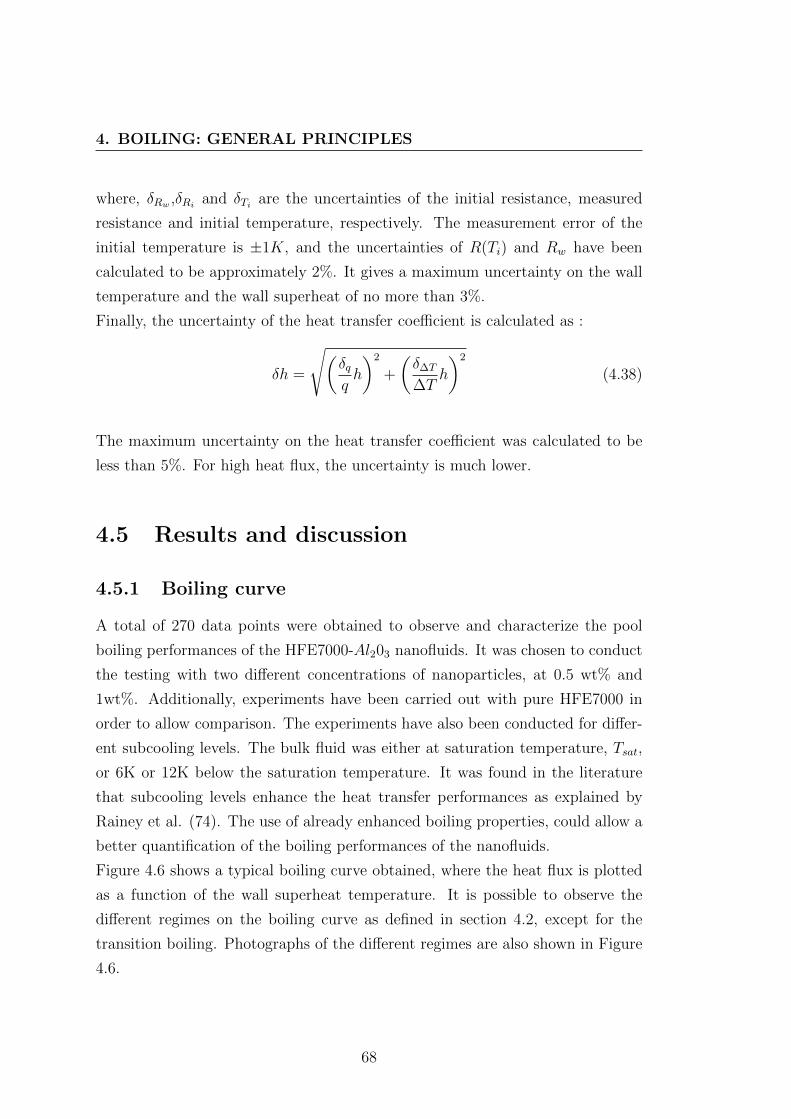
4. BOILING: GENERAL PRINCIPLES
where, δRw ,δRi and δTi are the uncertainties of the initial resistance, measured
resistance and initial temperature, respectively. The measurement error of the
initial temperature is ±1K, and the uncertainties of R(Ti) and Rw have been
calculated to be approximately 2%. It gives a maximum uncertainty on the wall
temperature and the wall superheat of no more than 3%.
Finally, the uncertainty of the heat transfer coefficient is calculated as :
δh =
√(δqqh
)2
+
(δ∆T
∆Th
)2
(4.38)
The maximum uncertainty on the heat transfer coefficient was calculated to be
less than 5%. For high heat flux, the uncertainty is much lower.
4.5 Results and discussion
4.5.1 Boiling curve
A total of 270 data points were obtained to observe and characterize the pool
boiling performances of the HFE7000-Al203 nanofluids. It was chosen to conduct
the testing with two different concentrations of nanoparticles, at 0.5 wt% and
1wt%. Additionally, experiments have been carried out with pure HFE7000 in
order to allow comparison. The experiments have also been conducted for differ-
ent subcooling levels. The bulk fluid was either at saturation temperature, Tsat,
or 6K or 12K below the saturation temperature. It was found in the literature
that subcooling levels enhance the heat transfer performances as explained by
Rainey et al. (74). The use of already enhanced boiling properties, could allow a
better quantification of the boiling performances of the nanofluids.
Figure 4.6 shows a typical boiling curve obtained, where the heat flux is plotted
as a function of the wall superheat temperature. It is possible to observe the
different regimes on the boiling curve as defined in section 4.2, except for the
transition boiling. Photographs of the different regimes are also shown in Figure
4.6.
68
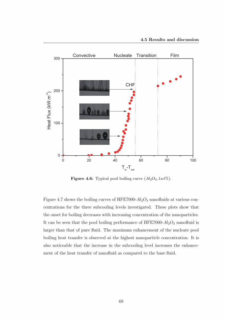
4.5 Results and discussion
Figure 4.6: Typical pool boiling curve (Al2O3, 1wt%).
Figure 4.7 shows the boiling curves of HFE7000-Al2O3 nanofluids at various con-
centrations for the three subcooling levels investigated. These plots show that
the onset for boiling decreases with increasing concentration of the nanoparticles.
It can be seen that the pool boiling performance of HFE7000-Al2O3 nanofluid is
larger than that of pure fluid. The maximum enhancement of the nucleate pool
boiling heat transfer is observed at the highest nanoparticle concentration. It is
also noticeable that the increase in the subcooling level increases the enhance-
ment of the heat transfer of nanofluid as compared to the base fluid.
69
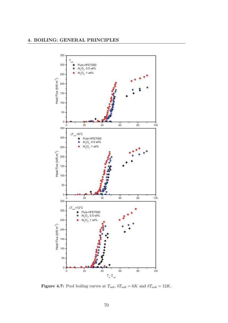
4. BOILING: GENERAL PRINCIPLES
Figure 4.7: Pool boiling curves at Tsat, δTsub = 6K and δTsub = 12K.
70
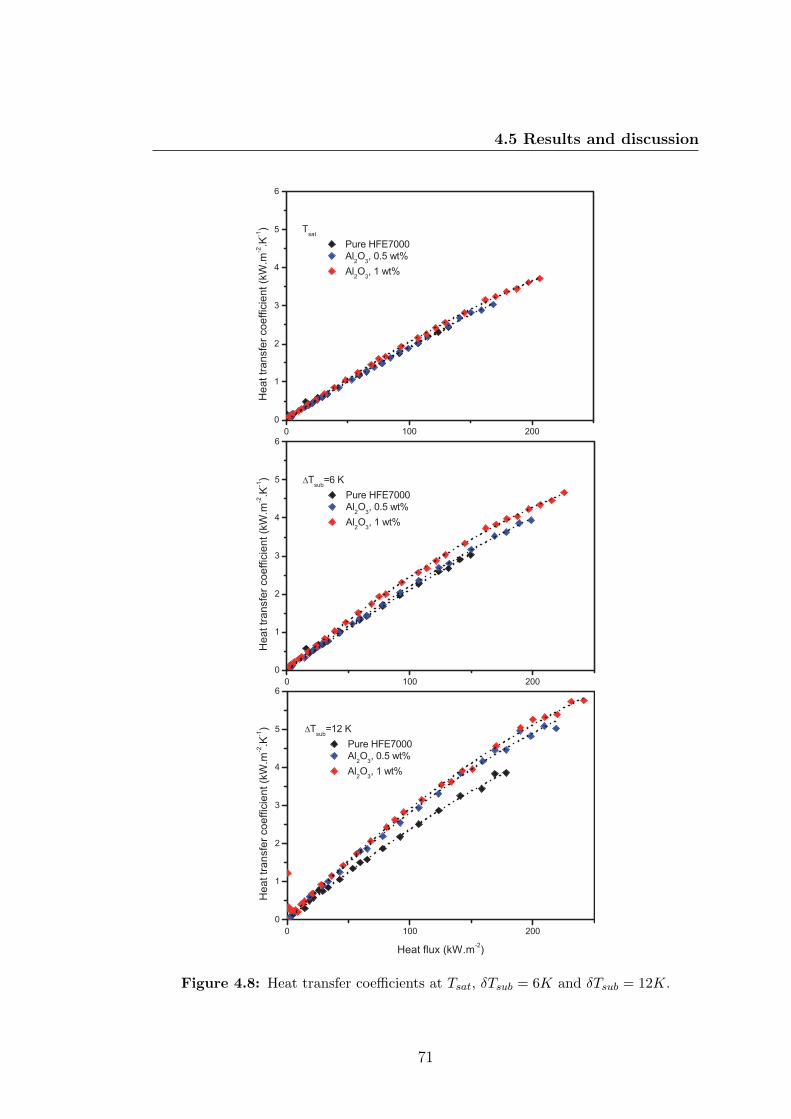
4.5 Results and discussion
Figure 4.8: Heat transfer coefficients at Tsat, δTsub = 6K and δTsub = 12K.
71
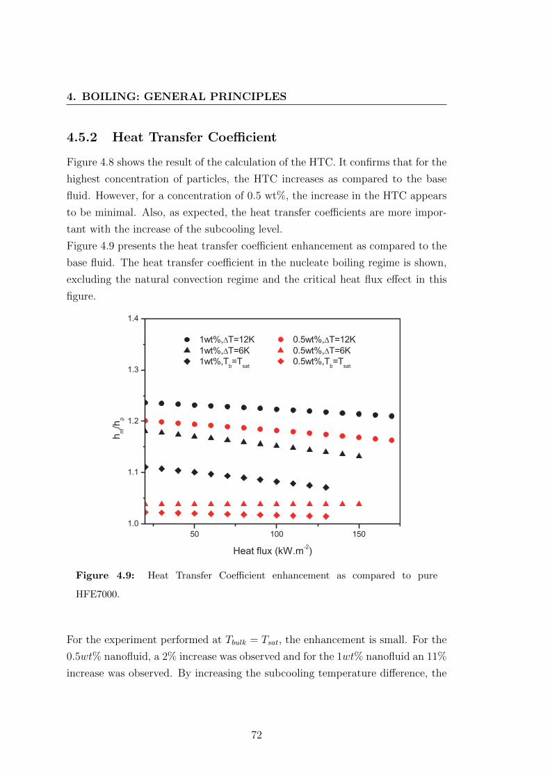
4. BOILING: GENERAL PRINCIPLES
4.5.2 Heat Transfer Coefficient
Figure 4.8 shows the result of the calculation of the HTC. It confirms that for the
highest concentration of particles, the HTC increases as compared to the base
fluid. However, for a concentration of 0.5 wt%, the increase in the HTC appears
to be minimal. Also, as expected, the heat transfer coefficients are more impor-
tant with the increase of the subcooling level.
Figure 4.9 presents the heat transfer coefficient enhancement as compared to the
base fluid. The heat transfer coefficient in the nucleate boiling regime is shown,
excluding the natural convection regime and the critical heat flux effect in this
figure.
Figure 4.9: Heat Transfer Coefficient enhancement as compared to pure
HFE7000.
For the experiment performed at Tbulk = Tsat, the enhancement is small. For the
0.5wt% nanofluid, a 2% increase was observed and for the 1wt% nanofluid an 11%
increase was observed. By increasing the subcooling temperature difference, the
72

4.5 Results and discussion
enhancement in the HTC was shown to be larger. For ∆Tsub = 6K, enhancements
are observed by 4% and 18% at concentration of 0.5wt% and 1wt%, respectively.
For ∆Tsub = 12K, a much larger increase in the heat transfer coefficient is ob-
served; enhancements are observed by up to 20% and 23% at concentration of
0.5wt% and 1wt%, respectively.
For the lowest concentration in nanoparticles, the enhancement is not significant
and falls in the uncertainty domain calculated previously. However, with the
highest concentration, the enhancement is clear. It is similar to those obtained
in experiments found in the literature such as Wen and Ding (56) who reported
enhancement by 30% with 2 % aluminum oxide nanofluid (but in a different base
fluid). Table 4.2 gives an overview of the maximum enhancement observed in this
research.
Table 4.2: Maximum enhancement of the heat transfer coefficient obtained in this
research
Tb = Tsat ∆Tsub = 6K ∆Tsub = 12K
0.5 wt% ≈ 2% ≈ 4% up to 20%
1 wt% up to 11% up to 18% up to 23%
The main hypotheses for the changes in the heat transfer coefficient are that the
thermophysical properties of the fluid are modified and enhanced as compared
to the base fluid and that the heating surface is modified due to the interaction
between the heating surface and the nanoparticles.
It was shown in the previous chapter that the thermophysical properties of the
nanofluids are similar to that of the base fluid, while the thermal conductivity
was expected to be higher. However, this increase in the thermal conductivity
was not observed with the nanofluids used in this research, and cannot explain
the increase in the heat transfer coefficient. Calculations on the heat transfer
coefficient, based on existing models, have shown that the thermal properties of
the nanofluids have a very limited effect.
73
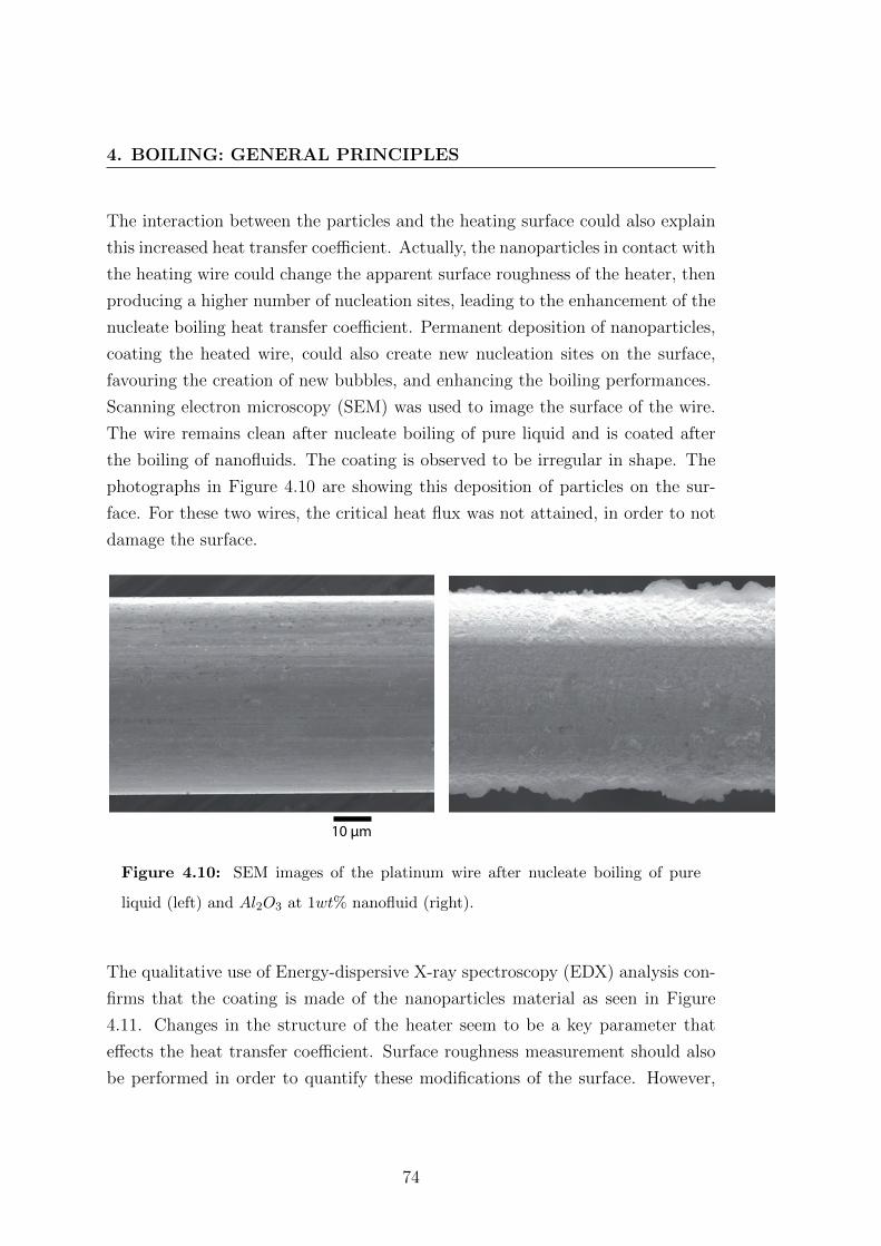
4. BOILING: GENERAL PRINCIPLES
The interaction between the particles and the heating surface could also explain
this increased heat transfer coefficient. Actually, the nanoparticles in contact with
the heating wire could change the apparent surface roughness of the heater, then
producing a higher number of nucleation sites, leading to the enhancement of the
nucleate boiling heat transfer coefficient. Permanent deposition of nanoparticles,
coating the heated wire, could also create new nucleation sites on the surface,
favouring the creation of new bubbles, and enhancing the boiling performances.
Scanning electron microscopy (SEM) was used to image the surface of the wire.
The wire remains clean after nucleate boiling of pure liquid and is coated after
the boiling of nanofluids. The coating is observed to be irregular in shape. The
photographs in Figure 4.10 are showing this deposition of particles on the sur-
face. For these two wires, the critical heat flux was not attained, in order to not
damage the surface.
10 µm
Figure 4.10: SEM images of the platinum wire after nucleate boiling of pure
liquid (left) and Al2O3 at 1wt% nanofluid (right).
The qualitative use of Energy-dispersive X-ray spectroscopy (EDX) analysis con-
firms that the coating is made of the nanoparticles material as seen in Figure
4.11. Changes in the structure of the heater seem to be a key parameter that
effects the heat transfer coefficient. Surface roughness measurement should also
be performed in order to quantify these modifications of the surface. However,
74
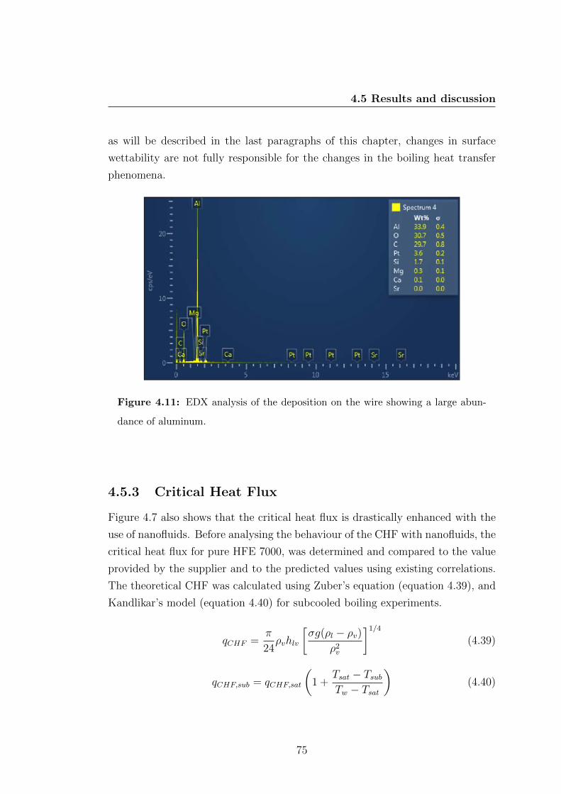
4.5 Results and discussion
as will be described in the last paragraphs of this chapter, changes in surface
wettability are not fully responsible for the changes in the boiling heat transfer
phenomena.
Figure 4.11: EDX analysis of the deposition on the wire showing a large abun-
dance of aluminum.
4.5.3 Critical Heat Flux
Figure 4.7 also shows that the critical heat flux is drastically enhanced with the
use of nanofluids. Before analysing the behaviour of the CHF with nanofluids, the
critical heat flux for pure HFE 7000, was determined and compared to the value
provided by the supplier and to the predicted values using existing correlations.
The theoretical CHF was calculated using Zuber’s equation (equation 4.39), and
Kandlikar’s model (equation 4.40) for subcooled boiling experiments.
qCHF =π
24ρvhlv
[σg(ρl − ρv)
ρ2v
]1/4
(4.39)
qCHF,sub = qCHF,sat
(1 +
Tsat − TsubTw − Tsat
)(4.40)
75
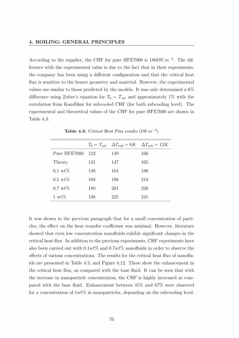
4. BOILING: GENERAL PRINCIPLES
According to the supplier, the CHF for pure HFE7000 is 180kW.m−2. The dif-
ference with the experimental value is due to the fact that in their experiments,
the company has been using a different configuration and that the critical heat
flux is sensitive to the heater geometry and material. However, the experimental
values are similar to those predicted by the models. It was only determined a 6%
difference using Zuber’s equation for Tb = Tsat and approximately 1% with the
correlation from Kandlikar for subcooled CHF (for both subcooling level). The
experimental and theoretical values of the CHF for pure HFE7000 are shown in
Table 4.3.
Table 4.3: Critical Heat Flux results (kW.m−2)
Tb = Tsat ∆Tsub = 6K ∆Tsub = 12K
Pure HFE7000 123 149 166
Theory 131 147 165
0.1 wt% 138 164 186
0.5 wt% 168 198 218
0.7 wt% 180 201 226
1 wt% 198 225 241
It was shown in the previous paragraph that for a small concentration of parti-
cles, the effect on the heat transfer coefficient was minimal. However, literature
showed that even low concentration nanofluids exhibit significant changes in the
critical heat flux. In addition to the previous experiments, CHF experiments have
also been carried out with 0.1wt% and 0.7wt% nanofluids in order to observe the
effects of various concentrations. The results for the critical heat flux of nanoflu-
ids are presented in Table 4.3, and Figure 4.12. These show the enhancement in
the critical heat flux, as compared with the base fluid. It can be seen that with
the increase in nanoparticle concentration, the CHF is highly increased as com-
pared with the base fluid. Enhancement between 45% and 67% were observed
for a concentration of 1wt% in nanoparticles, depending on the subcooling level.
76
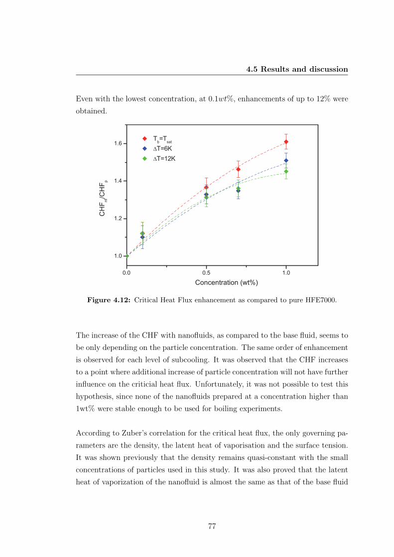
4.5 Results and discussion
Even with the lowest concentration, at 0.1wt%, enhancements of up to 12% were
obtained.
Figure 4.12: Critical Heat Flux enhancement as compared to pure HFE7000.
The increase of the CHF with nanofluids, as compared to the base fluid, seems to
be only depending on the particle concentration. The same order of enhancement
is observed for each level of subcooling. It was observed that the CHF increases
to a point where additional increase of particle concentration will not have further
influence on the criticial heat flux. Unfortunately, it was not possible to test this
hypothesis, since none of the nanofluids prepared at a concentration higher than
1wt% were stable enough to be used for boiling experiments.
According to Zuber’s correlation for the critical heat flux, the only governing pa-
rameters are the density, the latent heat of vaporisation and the surface tension.
It was shown previously that the density remains quasi-constant with the small
concentrations of particles used in this study. It was also proved that the latent
heat of vaporization of the nanofluid is almost the same as that of the base fluid
77
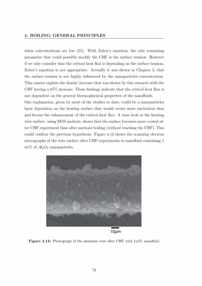
4. BOILING: GENERAL PRINCIPLES
when concentrations are low (55). With Zuber’s equation, the only remaining
parameter that could possibly modify the CHF is the surface tension. However
if we only consider that the critical heat flux is depending on the surface tension,
Zuber’s equation is not appropriate. Actually it was shown in Chapter 3, that
the surface tension is not highly influenced by the nanoparticles concentration.
This cannot explain the drastic increase that was shown by this research with the
CHF having a 67% increase. These findings indicate that the critical heat flux is
not dependent on the general thermophysical properties of the nanofluids.
One explanation, given by most of the studies to date, could be a nanoparticles
layer deposition on the heating surface that would create more nucleation sites
and favour the enhancement of the critical heat flux. A close look at the heating
wire surface, using SEM analysis, shows that the surface becomes more coated af-
ter CHF experiment than after nucleate boiling (without reaching the CHF). This
could confirm the previous hypothesis. Figure 4.13 shows the scanning electron
micrographs of the wire surface after CHF experiments in nanofluid containing 1
wt% of Al2O3 nanoparticles.
10µm
Figure 4.13: Photograph of the platinum wire after CHF with 1wt% nanofluid.
78
4.5 Results and discussion
It is hypothesized that this layer is due to precipitation of the particles caused
by nucleate boiling. As will be explained further in detail in the next chapter, it
is well known that a thin microlayer is created under the vapour bubble during
its nucleation and growth. The coating of the surface by the particles could be
the direct consequence of the evaporation of this thin microlayer, thus depositing
the particles contained in it. This particle deposition would be the reason for the
sharp increase of the critical heat flux, since it was reported in the literature that
changes in the surface configuration, roughness and wettability delay the CHF.
The effect of wettability changes can be investigated using the model proposed
by Kandlikar, which takes into account the contact angle at the liquid vapour
interface as shown by equation 4.41 below (50).
qCHF = hlvρ1/2v
(1 + cosθ
16
)[2
π+π
4(1 + cosθ)cosβ
]1/2
[σg(ρl − ρv)]1/4 (4.41)
According to this equation, a decrease in the contact angle leads to the increase
in the CHF. Deposition of nanoparticles on the surface, modifying the contact
angle, could then be the reason for the critical heat flux enhancement observed
in all the data, including this work. Results found in the literature, show that
the deposition of nanoparticles on the heating surface decreases the apparent
contact angle (75). They found that the contact angle of a 1µl water droplet
was decreased from 68 to 16 when measured on a clean heater or coated after
nanofluid boiling, respectively. This behaviour would result in the enhancement
of the critical heat flux.
However, HFE7000 is a highly wetting fluid, meaning that the contact angle
is very low. Equation 4.41 already fails in predicting the CHF for pure liquid.
To have a critical heat flux similar to the one observed experimentally and also
predicted by Zuber’s equation, the contact angle would be approximately 80.
The experimental measure of the contact angle resulted in a value close to 12 for
pure liquid on a clean surface and 9 on a surface where CHF experiments with
1wt% nanofluid have been performed (Figure 4.14). This small difference in the
contact angle is not significant in explaining the major difference between boiling
79
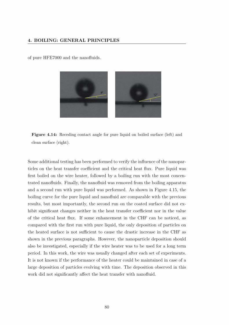
4. BOILING: GENERAL PRINCIPLES
of pure HFE7000 and the nanofluids.
9°12°
Figure 4.14: Receding contact angle for pure liquid on boiled surface (left) and
clean surface (right).
Some additional testing has been performed to verify the influence of the nanopar-
ticles on the heat transfer coefficient and the critical heat flux. Pure liquid was
first boiled on the wire heater, followed by a boiling run with the most concen-
trated nanofluids. Finally, the nanofluid was removed from the boiling apparatus
and a second run with pure liquid was performed. As shown in Figure 4.15, the
boiling curve for the pure liquid and nanofluid are comparable with the previous
results, but most importantly, the second run on the coated surface did not ex-
hibit significant changes neither in the heat transfer coefficient nor in the value
of the critical heat flux. If some enhancement in the CHF can be noticed, as
compared with the first run with pure liquid, the only deposition of particles on
the heated surface is not sufficient to cause the drastic increase in the CHF as
shown in the previous paragraphs. However, the nanoparticle deposition should
also be investigated, especially if the wire heater was to be used for a long term
period. In this work, the wire was usually changed after each set of experiments.
It is not known if the performance of the heater could be maintained in case of a
large deposition of particles evolving with time. The deposition observed in this
work did not significantly affect the heat transfer with nanofluid.
80
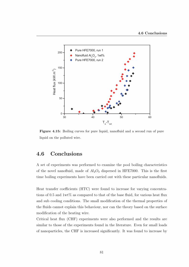
4.6 Conclusions
Figure 4.15: Boiling curves for pure liquid, nanofluid and a second run of pure
liquid on the polluted wire.
4.6 Conclusions
A set of experiments was performed to examine the pool boiling characteristics
of the novel nanofluid, made of Al2O3 dispersed in HFE7000. This is the first
time boiling experiments have been carried out with these particular nanofluids.
Heat transfer coefficients (HTC) were found to increase for varying concentra-
tions of 0.5 and 1wt% as compared to that of the base fluid, for various heat flux
and sub cooling conditions. The small modification of the thermal properties of
the fluids cannot explain this behaviour, nor can the theory based on the surface
modification of the heating wire.
Critical heat flux (CHF) experiments were also performed and the results are
similar to those of the experiments found in the literature. Even for small loads
of nanoparticles, the CHF is increased significantly. It was found to increase by
81
4. BOILING: GENERAL PRINCIPLES
67% for the nanofluid with 1wt% of Al2O3 dispersed in HFE7000. This shows
the potential of such nanofluids for industrial applications, since it could increase
the upper limit of safe applications. However, in the same manner as for the heat
transfer coefficient, the theory based on the surface modification improving the
CHF, is not sufficient. It was shown that surface modification has an impact on
nucleate pool boiling. But this is not the only governing parameter that leads to
an increase in the HTC and CHF. Models and correlations proposed in the liter-
ature did not reflect the effect of the nanoparticles on the boiling performances.
This problem required a more fundamental approach of the heat and mass trans-
fer occurring during the boiling process. A closer look at the interactions between
the nanoparticles and the formation and growth of the vapour bubbles could help
in understanding the inconsistencies found in the literature and are not explained
with general boiling theories. A study at a smaller scale, focusing on the inter-
action of the nanofluid with the dynamic of the bubbles created during nucleate
boiling, is of high importance. The study of the nucleation, growth and detach-
ment dynamic of single vapour bubbles is presented in the following chapter.
82
5
Boiling at a reduced scale: single
vapour bubble
5.1 Introduction
As shown in the previous chapter, nucleate boiling heat transfer is influenced by
several parameters and experimental conditions. Models presented in the liter-
ature and experimental theories proposed, do not fully explain the mechanisms
responsible for the enhancement or deterioration of the heat transfer coefficient
and critical heat flux using nanofluids. This requires a more fundamental ap-
proach to the heat and mass transfer during boiling. For that purpose, the study
of the growth of single vapour bubbles is presented in the following chapter.
Studies of isolated bubble growth allow focusing at a smaller scale on the local
heat transfer and hiding some mechanisms such as the interaction between the
bubbles. The chapter begins with a description of the mechanisms of formation
and growth of vapour bubbles and presents the experimental apparatus based on
a Hele-shaw cell model, where the growth dynamic of a vapour bubble in pure
liquid and nanofluid is studied.
83
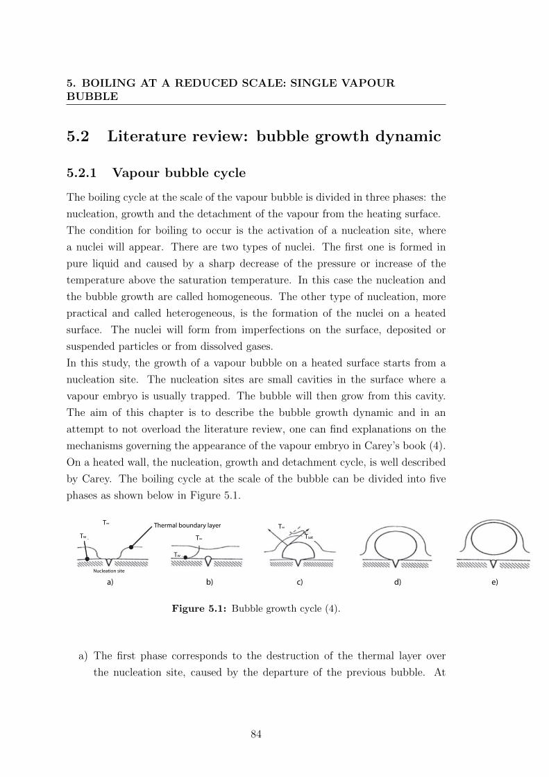
5. BOILING AT A REDUCED SCALE: SINGLE VAPOURBUBBLE
5.2 Literature review: bubble growth dynamic
5.2.1 Vapour bubble cycle
The boiling cycle at the scale of the vapour bubble is divided in three phases: the
nucleation, growth and the detachment of the vapour from the heating surface.
The condition for boiling to occur is the activation of a nucleation site, where
a nuclei will appear. There are two types of nuclei. The first one is formed in
pure liquid and caused by a sharp decrease of the pressure or increase of the
temperature above the saturation temperature. In this case the nucleation and
the bubble growth are called homogeneous. The other type of nucleation, more
practical and called heterogeneous, is the formation of the nuclei on a heated
surface. The nuclei will form from imperfections on the surface, deposited or
suspended particles or from dissolved gases.
In this study, the growth of a vapour bubble on a heated surface starts from a
nucleation site. The nucleation sites are small cavities in the surface where a
vapour embryo is usually trapped. The bubble will then grow from this cavity.
The aim of this chapter is to describe the bubble growth dynamic and in an
attempt to not overload the literature review, one can find explanations on the
mechanisms governing the appearance of the vapour embryo in Carey’s book (4).
On a heated wall, the nucleation, growth and detachment cycle, is well described
by Carey. The boiling cycle at the scale of the bubble can be divided into five
phases as shown below in Figure 5.1.
Thermal boundary layer T
Tw
T∞
Tw
T∞
T∞
Tsat
Nucleation site
b) e)d)a) c)
Figure 5.1: Bubble growth cycle (4).
a) The first phase corresponds to the destruction of the thermal layer over
the nucleation site, caused by the departure of the previous bubble. At
84
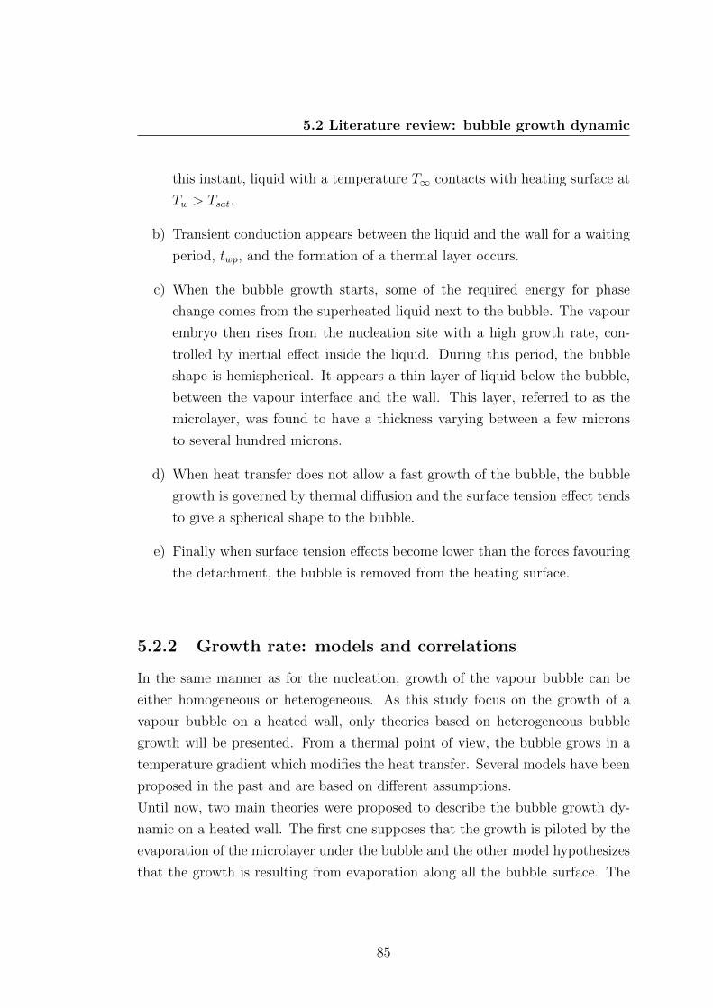
5.2 Literature review: bubble growth dynamic
this instant, liquid with a temperature T∞ contacts with heating surface at
Tw > Tsat.
b) Transient conduction appears between the liquid and the wall for a waiting
period, twp, and the formation of a thermal layer occurs.
c) When the bubble growth starts, some of the required energy for phase
change comes from the superheated liquid next to the bubble. The vapour
embryo then rises from the nucleation site with a high growth rate, con-
trolled by inertial effect inside the liquid. During this period, the bubble
shape is hemispherical. It appears a thin layer of liquid below the bubble,
between the vapour interface and the wall. This layer, referred to as the
microlayer, was found to have a thickness varying between a few microns
to several hundred microns.
d) When heat transfer does not allow a fast growth of the bubble, the bubble
growth is governed by thermal diffusion and the surface tension effect tends
to give a spherical shape to the bubble.
e) Finally when surface tension effects become lower than the forces favouring
the detachment, the bubble is removed from the heating surface.
5.2.2 Growth rate: models and correlations
In the same manner as for the nucleation, growth of the vapour bubble can be
either homogeneous or heterogeneous. As this study focus on the growth of a
vapour bubble on a heated wall, only theories based on heterogeneous bubble
growth will be presented. From a thermal point of view, the bubble grows in a
temperature gradient which modifies the heat transfer. Several models have been
proposed in the past and are based on different assumptions.
Until now, two main theories were proposed to describe the bubble growth dy-
namic on a heated wall. The first one supposes that the growth is piloted by the
evaporation of the microlayer under the bubble and the other model hypothesizes
that the growth is resulting from evaporation along all the bubble surface. The
85
5. BOILING AT A REDUCED SCALE: SINGLE VAPOURBUBBLE
following paragraphs describe some of these models. Only the main models are
presented, since various other models exist, based on the same assumptions, but
only some parameters have been modified.
5.2.2.1 Bubble growth by evaporation of the microlayer
During the first moment of growth, the bubble grows rapidly, leading to the
trapping of a thin layer of liquid under the bubble. The evaporation of this
microlayer is then responsible for the growth of the bubble. The first model was
developed by Cooper and Loyd (76). They considered the growth due to the
expansion of the dry area under the vapour bubble and by the growth of the
bubble radius as described by equation 5.1:
R(t) = C.tn (5.1)
where C and n are constant. R is the bubble radius and t is the time. The value
of n is usually between 0.3 and 0.7. The initial thickness of the microlayer can
be estimated assuming a spherical bubble and is given by:
δ0 = C√νlt (5.2)
where C is a constant with an approximate value of 0.8 in the model (from 0.5
to 1 in their experimental results). It was shown later that C is not constant but
decreases with time due to surface tension which is neglected in the model.
For a hemispherical bubble, Cooper proposed two models whose validity depends
on the thermal conductivities of the wall, λw and the liquid, λl (45). It is assumed
that the wall temperature remains constant during evaporation of the microlayer.
The liquid-vapour interface temperature is supposed to be at saturation and the
heat transfers are assumed to be purely conductive. In this case, the bubble
growth is given by:
86
5.2 Literature review: bubble growth dynamic
if λw >> λl
R(t) = 2.5Jal
√αlt
Prl(5.3)
if λw << λl
R(t) =2√π
√λpρwCpwλlρlCpl
Jal√αlt (5.4)
Another model was proposed by Van Ouwerkerk, in which the thermal properties
of the wall and the specific heat of the microlayer are taken into account (77).
The following equation proposes an analytical solution for a particular case. The
shape of the bubble is assumed to be identical at all stages of the growth, the
wall temperature remains constant and the liquid is slightly overheated.
Then, for the terms√
λpρwCpwλlρlCpl
= 1 and Cp(T0−Tsat)hlv
having a low value, the bubble
growth is defined by:
R(t) = C√t (5.5)
with:
C =2(1 +
√3)√
πJal√αl (5.6)
T0 is, in that case, the initial temperature of the microlayer and is equal to the
wall temperature.
Finally, Cooper and Merry also took into account the temperature variation of
the wall, and the calorific capacity of the liquid (78). Assuming that, for an
hemispherical bubble, the radius evolution is R(t) ∼ tn, they obtained:
R(t) =3
2Cρlρv
√(νlt)I (5.7)
where I is integrating the temporal evolution of the microlayer and C is given by
C = δ0√νlt
(equation 5.2).
87
5. BOILING AT A REDUCED SCALE: SINGLE VAPOURBUBBLE
5.2.2.2 Growth by evaporation on all the bubble surface
The other theory hypothesizes that the bubble growth dynamic is governed by
the evaporation on all the bubble surface.
Mikic and Roshenhow treated the problem in two parts (79). The first phase cor-
responded to a process of instationary conduction in the liquid, the second phase
to the bubble growth. During the waiting time, twp, the instationary conduction
in the liquid is assumed to be governed by the heat equation. In that case, the
radius of the vapour bubble is given by equation 5.8:
R(t) =2Jal√
3πλlt
π
(1 +
Tw − T∞Tw − Tsat
([1 +
twpt
]1/2
−[twpt
]1/2))
(5.8)
In order to determine the waiting time, the authors supposed that the tempera-
ture of the hemispheric vapour bubble is higher than the temperature required to
induce the bubble growth. They used the temperature profile during the waiting
period and obtained the following expression of the waiting time (rc is the radius
of the nucleation site).
twp =1
4αL
rc
erfc−1(Tsat(P0)−T0Tw−T0 + 2σTsat(P0)
(Tw−T0)rcρvhlv
) (5.9)
erfc(K) = 1− erf(K) = 1− 2√π
∫ K0exp(−x2)dx
Another approach used by Mikic and Roshenhow considered a bubble growing in
a uniformly superheated liquid (80). The authors developed a relation applicable
to the entire range of the growth, including the growth controlled by inertia and
by diffusion. They obtained a relation between the temperature and the pressure
by using a linearized version of Clausius-Clapeyron’s equation and supposed the
radius evolution to fit Rayleigh’s solution. They finally obtained the following
model:
R(t) =2B2
3A
([AB
]2
t+ 1
)3/2
−
([A
B
]2
t
)3/2
− 1
(5.10)
88
5.2 Literature review: bubble growth dynamic
where,
A =
(bhlvρv(Tl∞ − Tsat)
ρlTsat
)1/2
(5.11)
and
B =
(12alπ
)1/2
Jal (5.12)
with, b, a constant depending on the heating conditions. b equals 23
if the bubbles
grow in an infinite medium and b = π7
if growing on a heating surface. For short
times, equation 5.10 is simplified as R(t) = At, while for long times it can be
written as R(t) = B√t.
This model was then extended by several researchers, in order to take into ac-
count different parameters such as the variation of the vapour density, which was
shown later to highly influence the bubble growth rate when superheating in the
liquid is important (81, 82).
5.2.2.3 Growth by combining the two theories
There is finally a third approach to determine the bubble growth dynamic. It is
based on both of the theories presented before. It was shown that if the bubble
is smaller than the thickness of the thermal boundary layer, the bubble growth
could be governed by the evaporation of the microlayer and all around the bubble,
simultaneously. In that case, when the evaporation around the vapour bubble is
not negligible in front of the microlayer evaporation, Cooper modified the previ-
ous equations 5.28 and 5.4 (76). They become:
if λw >> λl
R(t) = 2.5Jaw
√αlt
Pr+ 2
√3
πJal√αlt (5.13)
if λw << λl
R(t) =2√π
√λwρwCwλlρlCl
Jaw√αlt+ 2
√3
πJal√αlt (5.14)
89
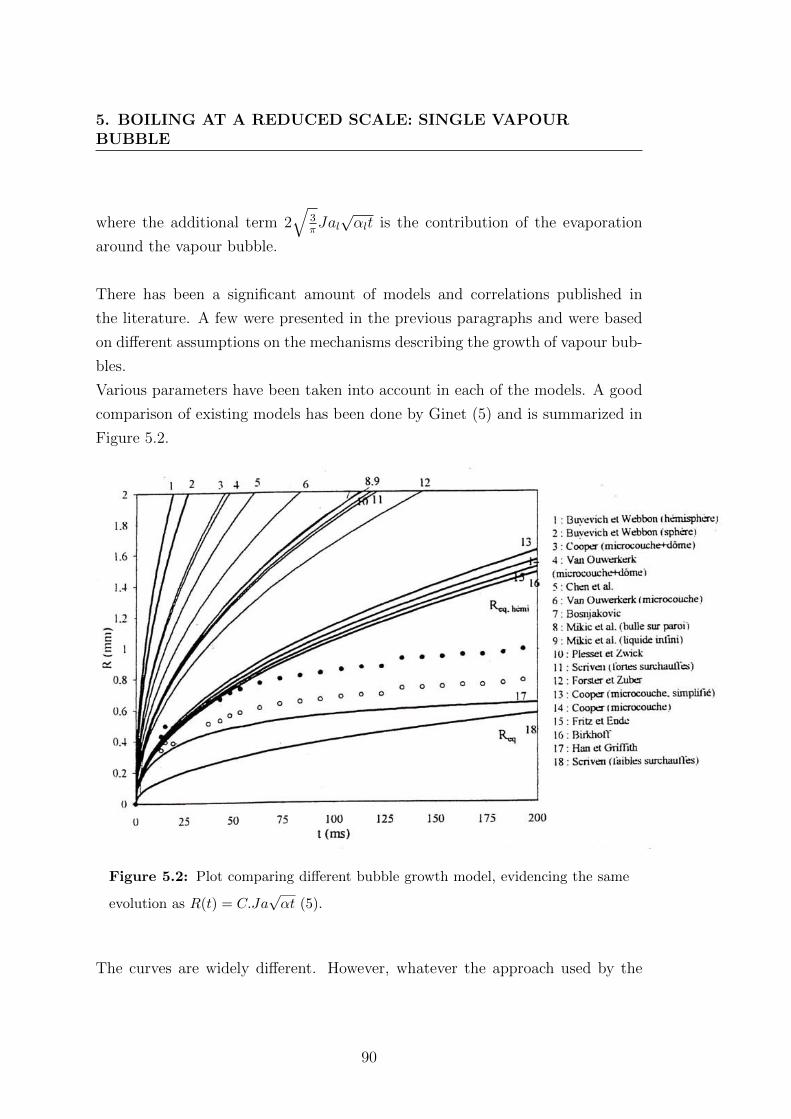
5. BOILING AT A REDUCED SCALE: SINGLE VAPOURBUBBLE
where the additional term 2√
3πJal√αlt is the contribution of the evaporation
around the vapour bubble.
There has been a significant amount of models and correlations published in
the literature. A few were presented in the previous paragraphs and were based
on different assumptions on the mechanisms describing the growth of vapour bub-
bles.
Various parameters have been taken into account in each of the models. A good
comparison of existing models has been done by Ginet (5) and is summarized in
Figure 5.2.
Figure 5.2: Plot comparing different bubble growth model, evidencing the same
evolution as R(t) = C.Ja√αt (5).
The curves are widely different. However, whatever the approach used by the
90
5.2 Literature review: bubble growth dynamic
authors, evaporation of the microlayer, along all the bubble surface or both, the
evolution of the bubble radius is defined with a similar equation written as:
R(t) = C.Ja√αt (5.15)
In this study, the vapour bubble growth dynamic for pure liquid and nanofluid
will be compared to these models.
5.2.3 Bubble growth with nanofluids
While there has been a significant amount of research on the boiling of nanofluid,
focused on heat transfer performance including the critical heat flux and the heat
transfer coefficient, studies of the influence of nanoparticles on the bubble growth
are very limited. Most of studies found in the literature aim at describing the
surface modification or the interactions between the nanoparticles and the gas-
liquid-solid interfaces.
Vafaei et al. investigated the dynamic of gas bubbles in nanofluids made of
gold nanoparticles (83). The bubbles were not formed by boiling but gas was
injected in the liquid with a nozzle. They demonstrated that the nanoparticles
significantly affect the bubble growth because the triple line becomes modified by
spreading and the contact angle changes. They showed that the surface tension
was modified, and the changes in the bubble volume and height were mostly due
to the modification of the triple line area.
Bubble growth during boiling has been studied using pure liquid on nano coated
surfaces. This was investigated by Phan et al. (84). Effect of surface wetta-
bility was investigated for several surfaces with various nano-coatings, changing
the water contact angle. It was found that higher surface wettability increases
the bubble departure radius and decreases the bubble release frequency. They
demonstrated that the heat transfers increased with increase in wettability. How-
ever, as in most of the studies, the bubble’s characteristics were not investigated
during the full time of its growth.
91
5. BOILING AT A REDUCED SCALE: SINGLE VAPOURBUBBLE
Most studies found in the literature aim at describing the surface modification or
the interaction between the nanoparticles and the gas-liquid-solid interfaces. No
publications concentrate on the growth dynamic of vapour bubbles in a nanofluid
focusing on the thermal effects, inducing modification in the bubble’s behaviour
during its growth.
92
5.3 Experimental set-up
5.3 Experimental set-up
5.3.1 Hele-shaw cell
The design of the experimental cell, shown in Figure 5.3, is based on the Hele-
Shaw model, originally designed for the Nanosurf research project (ANR-09-
BLAN-0093-03), which consists of confining the liquid between two parallel plates,
and allowing a two dimension study of the boiling phenomena.
This kind of experimental configuration has already been used for various studies
such as the Marangoni effect, the mix of two miscible liquids or, more recently,
the growth of vapour bubbles (85, 86). Serret et al. studied the contact angle
variation of a 2D growing vapour bubble in a fluorinert FC-72 fluid in normal
gravity and reduced gravity using this kind of experimental design(87, 88). This
cell configuration has been chosen because its geometry will minimize problems
due to three dimensional effects. Since the bubbles are created and maintained in
the same plane during the nucleation-detachment cycle, optical aberrations due
to high thermal gradient in the thermal boundary close to the wall are avoided.
Barthes showed that the mirage effect produces a significant error in the interface
localization, while generating a vapour bubble on a downward facing element (89),
and Wen showed the limitations when video measurements are made through the
liquid to observe boiling (37).
The aim of this test cell is to generate successive bubbles on an artificial nu-
cleation site. This device makes it possible to control the parameters relating to
the heating and the fluid (inlet temperature in the cell, flow rate in entry of the
cell, heat flux). Schematics of the cell are shown below in Figure 5.3 and 5.4.
93
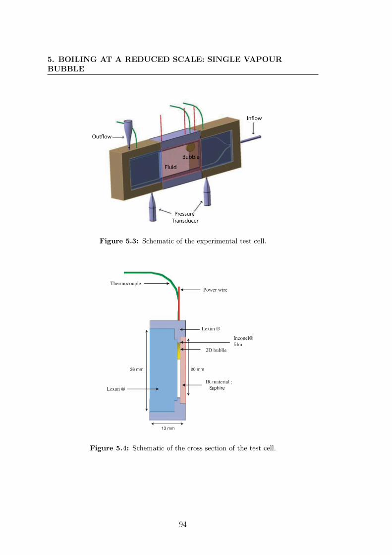
5. BOILING AT A REDUCED SCALE: SINGLE VAPOURBUBBLE
Bubble
Fluid
Pressure
Transducer
Out!ow
In!ow
Figure 5.3: Schematic of the experimental test cell.
20 mm 36 mm
13 mm
Lexan ®
Thermocouple
Power wire
Lexan ®
2D b u b lle
I nconel®
film
IR material :
Saphire
Figure 5.4: Schematic of the cross section of the test cell.
94
5.3 Experimental set-up
The cells were made out of polycarbonate with a side face in sapphire allowing
infrared visualization. The latter face is transparent to infrared (IR) radiation
and had been treated to obtain a transmitivity of 90%. The thickness between
the two parallel faces was 1mm and the heating was ensured by a film in Inconel
electrically powered on which a 50 µm triangular hole was drilled to create a
unique artificial nucleation site. The inconel film was 1cm× 1mm× 100µm, with
a resistance of 1Ω, and connected via two electrodes to an ISO-TECH IPS-405
stabilized power supply, delivering up to 40V and 5A.
The choice to have the heating element and the created bubble facing downward
was made for precision purposes. In order to have precise images of the bubble
growing, it is necessary to have a bubble as large as possible. With this con-
figuration, the bubble growth time and the bubble size will be larger than for
bubbles created on an upward facing heating surface. This configuration was also
justified because this experimental set-up was designed for research in micrograv-
ity, during a parabolic flight campaign, where normal gravity, hyper gravity and
reduced gravity could be obtained. If the vapour bubble was created over the
heating surface, the hyper gravity phases, and increased buoyancy would cause
the bubble to depart prematurely from the nucleation site.
5.3.2 Fluid loop
The experimental study of the nucleation and growth of a single vapour bubble
was undertaken in a fluid loop situated inside a confinement box. The box was
fully closed to avoid any contact with potential leaks in the fluid loop. A door
on its side, allowed access to the equipment and was maintained with latches. A
glove (the same model as on glove box) allowed it to work inside the confinement
box without opening it. It could also be used as a mobile membrane in case of
overpressure. The glove support was manufactured by Jacomex and allowed a
perfect tightness.
The confinement box was preheated at a temperature close to the fluid satu-
ration temperature. The temperature regulation was made through two 50W
Peltier elements controlled by two MPT10000 regulators from Wavelength Elec-
tronics. The desired temperature in the confinement box was set by supplying
95
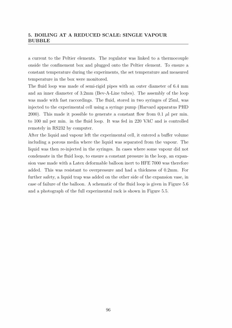
5. BOILING AT A REDUCED SCALE: SINGLE VAPOURBUBBLE
a current to the Peltier elements. The regulator was linked to a thermocouple
onside the confinement box and plugged onto the Peltier element. To ensure a
constant temperature during the experiments, the set temperature and measured
temperature in the box were monitored.
The fluid loop was made of semi-rigid pipes with an outer diameter of 6.4 mm
and an inner diameter of 3.2mm (Bev-A-Line tubes). The assembly of the loop
was made with fast raccordings. The fluid, stored in two syringes of 25ml, was
injected to the experimental cell using a syringe pump (Harvard apparatus PHD
2000). This made it possible to generate a constant flow from 0.1 µl per min.
to 100 ml per min. in the fluid loop. It was fed in 220 VAC and is controlled
remotely in RS232 by computer.
After the liquid and vapour left the experimental cell, it entered a buffer volume
including a porous media where the liquid was separated from the vapour. The
liquid was then re-injected in the syringes. In cases where some vapour did not
condensate in the fluid loop, to ensure a constant pressure in the loop, an expan-
sion vase made with a Latex deformable balloon inert to HFE 7000 was therefore
added. This was resistant to overpressure and had a thickness of 0.2mm. For
further safety, a liquid trap was added on the other side of the expansion vase, in
case of failure of the balloon. A schematic of the fluid loop is given in Figure 5.6
and a photograph of the full experimental rack is shown in Figure 5.5.
96
5.3 Experimental set-up
Co
mp
ute
r 1
: D
ata
ac
qu
isit
ion
Co
mp
ute
r 2
: In
fra
red
Ca
me
ra
Co
mp
ute
r 3
: Vis
ible
Ca
me
ra
Co
n!
ne
me
nt
Bo
x
Infr
are
d c
am
era
Vis
ible
ca
me
ra
Ex
pe
rim
en
tal
ce
ll
Sy
rin
gu
e p
um
p
Liq
uid
tra
p
Ex
pe
nsi
on
va
se
Sta
bil
ize
d p
ow
er
sup
ply
Ele
cti
ca
l P
an
el
Fig
ure
5.5
:P
hot
ogra
ph
sof
the
exp
erim
enta
lra
cksh
owin
gth
ege
ner
alas
pec
tof
the
exp
erim
ent,
the
contr
oll
ing
com
pu
ters
and
vid
eoac
qu
isit
ion
syst
ems.
97

5. BOILING AT A REDUCED SCALE: SINGLE VAPOURBUBBLE
Fig
ure
5.6
:S
chem
atic
ofth
eex
per
imen
tal
flu
idlo
opsh
owin
gth
ed
iffer
ent
app
aratu
sen
close
din
the
con
fin
emen
tb
ox.
98

5.3 Experimental set-up
5.3.3 Experimental procedure
The experimental procedure was simple.
1) The fluid was first in the buffer volume, and the confinement box was heated
over the saturation temperature. The fluid was left to boil for several min-
utes in order to remove the dissolved gases. The confinement box was then
heated close to the saturation temperature (typically 2 degrees below satu-
ration).
2) The two 25 mL syringes were filled.
3) A mass flow rate was set on the syringe pump (low flow rate, mostly to evac-
uate the vapour bubble) and a constant heat flux was set via the stabilized
power supply.
4) The data acquisition started after a steady state was achieved, when the
bubble creation and detachment frequency was stabilized.
5.3.4 Data acquisition
The data acquisition in this study was mainly based on temperature measure-
ments and geometric characteristics of the vapour bubble. Since thermocouples
would disturb the liquid flow and the bubble growth, the temperature measure-
ments were performed with infrared measurements. However, two K-type ther-
mocouples were included in the fluid loop. One was positioned in the pipe at
the entry of the test cell to ensure the temperature was as desired, a few de-
grees below the saturation temperature. The other thermocouple was positioned
above the nucleation site, and the measured temperature was used as a reference
for the infrared camera calibration. The acquisition system was a Texas Instru-
ment data acquisition system composed of a CompactDAQ chassis, a NI 9205
module(analogic 16 bits, 250 ks/s, +/- 10V, 32 channels), and a NI9213 module
(16-channel for thermocouples, 24 bits).
The visualization of the bubble growth was made simultaneously using infrared
and visible cameras. The two cameras were positioned on each side of the test
99
5. BOILING AT A REDUCED SCALE: SINGLE VAPOURBUBBLE
cell and perpendicular to the flow. The visible camera was a Canon EOS 7D,
coupled with a 5× magnification lens. The resolution of the video was 1280×720
at 50 frames per second. A cold light was also used to improve the contrast.
The infrared camera was a FLIR SC6000, with a resolution of 640 × 512 and a
capability of 126 frames per second.
5.3.5 Data processing
The combination of visible and infrared visualization enabled the observation of
the bubble growth and allowed access to the temperature field around the vapour
bubbles. The main thermal parameters extracted from the infrared visualization
were the temperature of the nucleation site, the temperature of the bubble inter-
face and the temperature of the liquid far from the bubble. Since the radiative
heat flux arriving at the infrared camera detector came from the heated liquid,
the data analysis was performed only in the liquid part and at the bubble inter-
face. Assuming a curved bubble interface in between the two Hele-Shaw plates,
the temperature coming from the interface came from the liquid side. No qual-
itative data analysis was performed using temperature coming from the inside
of the bubble because that region is vapour and has an undetermined emissiv-
ity. The infrared camera calibration was performed by comparing the fluid inlet
temperature, given by a thermocouple placed in the fluid loop, and the camera
temperature. The temperature difference between these two values was less than
0.1C.
The geometric characteristics, including the bubble diameter, the wetting diame-
ter (corresponding to the interface between the bubble and the heating surface),
the height and the contact angle were determined using the visible camera im-
ages. Using ImageJ (free image analysis software), the characteristic lengths were
obtained with a precision of ±10µm. The contact angle could also be determined
manually using this software. The measurement error due to the experimenta-
tion subjectivity makes this technique imprecise. The maximum diameter of the
bubble was less than the capillary length, Lc as well as the thickness of confine-
ment. The bubble was assumed to be axisymetric, with a spherical cap shape.
100
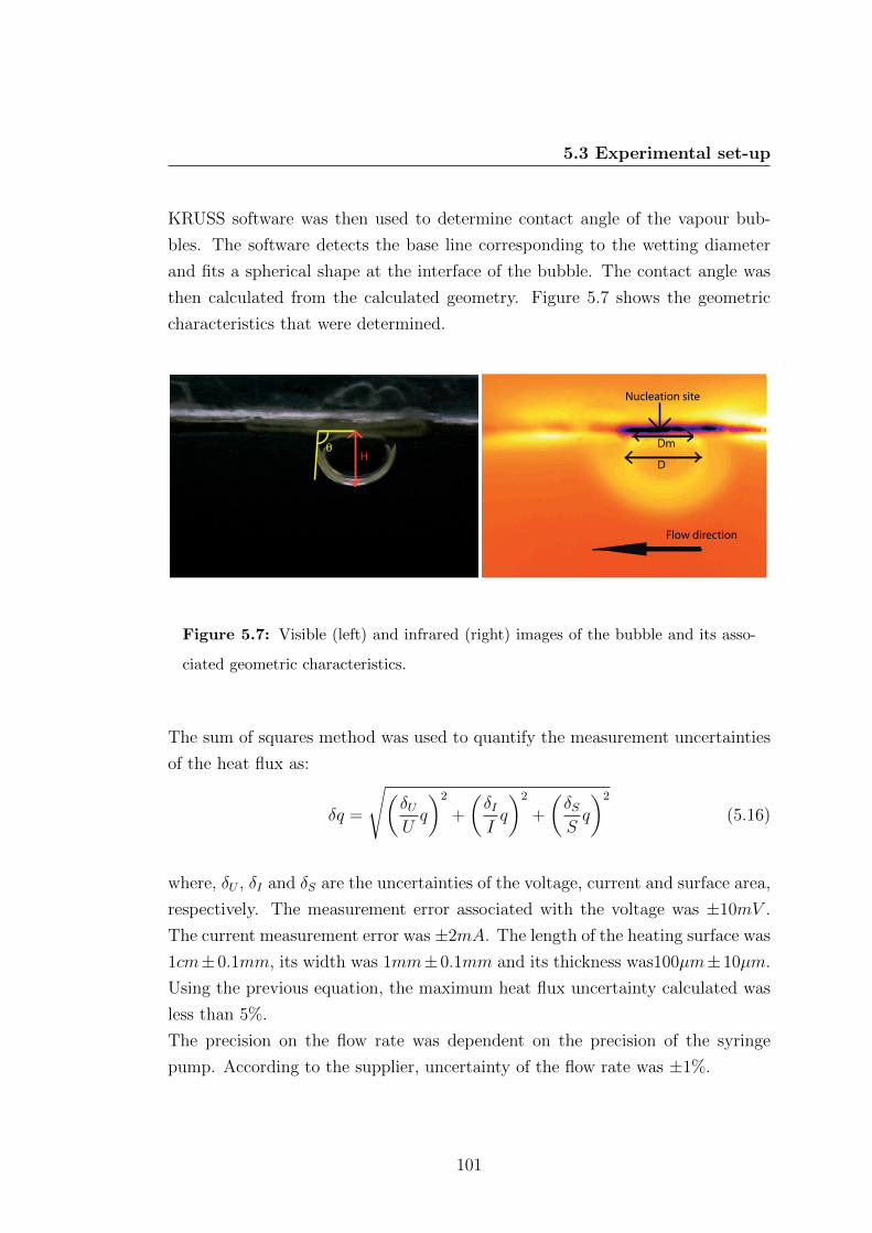
5.3 Experimental set-up
KRUSS software was then used to determine contact angle of the vapour bub-
bles. The software detects the base line corresponding to the wetting diameter
and fits a spherical shape at the interface of the bubble. The contact angle was
then calculated from the calculated geometry. Figure 5.7 shows the geometric
characteristics that were determined.
Dm
DH
θ
Flow direction
Nucleation site
Figure 5.7: Visible (left) and infrared (right) images of the bubble and its asso-
ciated geometric characteristics.
The sum of squares method was used to quantify the measurement uncertainties
of the heat flux as:
δq =
√(δUUq
)2
+
(δIIq
)2
+
(δSSq
)2
(5.16)
where, δU , δI and δS are the uncertainties of the voltage, current and surface area,
respectively. The measurement error associated with the voltage was ±10mV .
The current measurement error was ±2mA. The length of the heating surface was
1cm±0.1mm, its width was 1mm±0.1mm and its thickness was100µm±10µm.
Using the previous equation, the maximum heat flux uncertainty calculated was
less than 5%.
The precision on the flow rate was dependent on the precision of the syringe
pump. According to the supplier, uncertainty of the flow rate was ±1%.
101
5. BOILING AT A REDUCED SCALE: SINGLE VAPOURBUBBLE
5.4 Results and discussion
The local growth of single vapour bubbles in shear flow were investigated to
model different boiling situations, from pool boiling to convective boiling (in small
shear flow). The measurements and observations made, are at the bubble scale
and cover both hydrodynamic and heat transfer. The geometrical bubble growth
dynamic and the heat transfer at the bubble interface were investigated. The first
section only deals with the bubble growth of pure HFE7000, where the bubble
dynamic was investigated for several heat fluxes and mass flow rates. New results
of the geometric and thermal characteristics of the liquid-vapour interface have
been determined (Diana et al.(90)). The second section provides a comparison of
the bubble growth dynamic between pure liquid and HFE7000-Al2O3 at 1wt%.
This nanofluid showed the highest improvement in the heat transfer coefficient as
explained in the previous chapter. The bubble creation frequency, bubble growth
rate, the nucleation site and interface temperature were all examined.
5.4.1 Growth dynamic of pure liquid
For flow rates varying between 0.5 and 2 ml.min−1 and heat fluxes between
1 and 2 W.cm−2, thermal and geometrical characteristics are investigated and
lead to the determination of the bubble growth rate. It aims at validating the
experimental method only based on video acquisition. Actually, the growth rate
determined geometrically will be compared to the growth rate based on thermal
measurements.
5.4.1.1 Bubble release frequency
From the video analysis, the frequency of nucleation/detachment of the vapour
bubbles can be determined for the various heat fluxes and mass flow rates. The
visible video provided easy access to the bubble release frequency but the data
treatment was heavier compared with the infrared measurements (which give the
exact same results).
The analysis of the infrared video enabled determination of the temperature vari-
ations of the nucleation site when the bubble was created, growing and detaching.
102
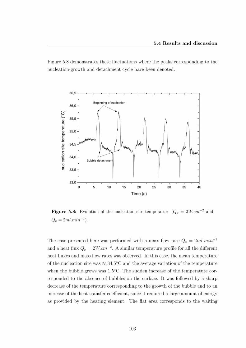
5.4 Results and discussion
Figure 5.8 demonstrates these fluctuations where the peaks corresponding to the
nucleation-growth and detachment cycle have been denoted.
Figure 5.8: Evolution of the nucleation site temperature (Qp = 2W.cm−2 and
Qv = 2ml.min−1).
The case presented here was performed with a mass flow rate Qv = 2ml.min−1
and a heat flux Qp = 2W.cm−2. A similar temperature profile for all the different
heat fluxes and mass flow rates was observed. In this case, the mean temperature
of the nucleation site was ≈ 34.5C and the average variation of the temperature
when the bubble grows was 1.5C. The sudden increase of the temperature cor-
responded to the absence of bubbles on the surface. It was followed by a sharp
decrease of the temperature corresponding to the growth of the bubble and to an
increase of the heat transfer coefficient, since it required a large amount of energy
as provided by the heating element. The flat area corresponds to the waiting
103

5. BOILING AT A REDUCED SCALE: SINGLE VAPOURBUBBLE
period between the detachment of a bubble and the nucleation of a new one. The
release frequency is defined as:
f =1
τg + τwp(5.17)
where τg and τwp are the bubble growth time and the waiting period, respectively.
In the presented case, τg = 1.2s and τwp = 5.5s, which gives an approximate
release frequency of 0.15 Hz.
In Figure 5.9, the nucleation frequency is compared for several heat flux and mass
flow rates.
Figure 5.9: Variation of the bubble detachment frequency as a function of the
mass flow rate and heat flux.
When the heat flux rises, an increase of the detachment frequency due to a faster
activation of the nucleation site was observed. In the same manner, an increase
104
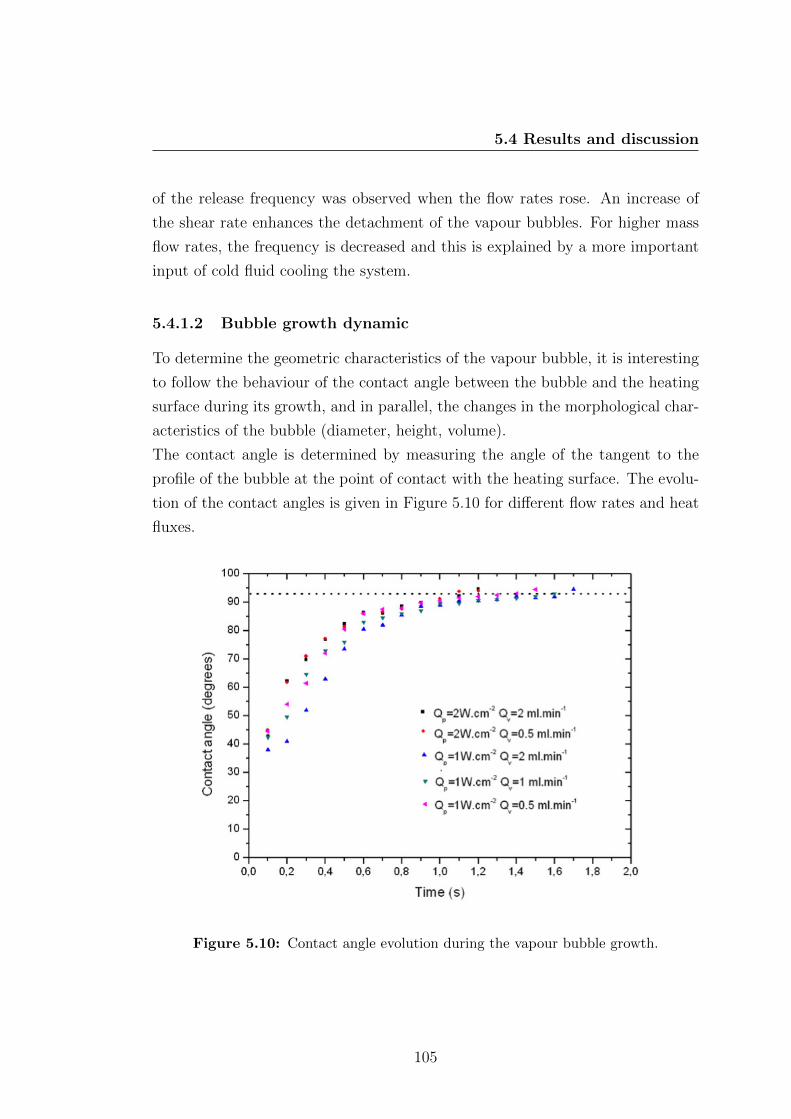
5.4 Results and discussion
of the release frequency was observed when the flow rates rose. An increase of
the shear rate enhances the detachment of the vapour bubbles. For higher mass
flow rates, the frequency is decreased and this is explained by a more important
input of cold fluid cooling the system.
5.4.1.2 Bubble growth dynamic
To determine the geometric characteristics of the vapour bubble, it is interesting
to follow the behaviour of the contact angle between the bubble and the heating
surface during its growth, and in parallel, the changes in the morphological char-
acteristics of the bubble (diameter, height, volume).
The contact angle is determined by measuring the angle of the tangent to the
profile of the bubble at the point of contact with the heating surface. The evolu-
tion of the contact angles is given in Figure 5.10 for different flow rates and heat
fluxes.
Figure 5.10: Contact angle evolution during the vapour bubble growth.
105
5. BOILING AT A REDUCED SCALE: SINGLE VAPOURBUBBLE
A variation of the contact angle was observed for two phases. Just after the
bubble nucleation and at early growth, the contact angle increased very rapidly
(t<0.8 s) to reach a plateau (t >0.8 s) around 90 where the angle stabilized. In
these experiments, whatever the heat flux or mass flow rate, the bubble detach-
ment occured with a similar contact angle .
Parallel to the contact angle measurements, the volume evolution of the bub-
ble was plotted. The data obtained with the camera visible, enabled precise
determination of the wetting diameter as well as the height of the bubble. As
the maximum diameter of the bubble was less than the capillary length Lc and
the thickness of confinement, the bubble was considered as axisymmetric and the
volume could be calculated as:
V (Rw, θ) =πR3
w
3
(1− cosθ)2(2 + cosθ)
sin3θ(5.18)
where, θ is the contact angle determined previously and Rw is the wetting radius
measured from the captured images.
A calculation of the volume based on the assumption that the vapour bubble
has the shape of a spherical cap, where the maximum diameter and height are
used, gave the same results as the calculation based on the wetting diameter and
contact angle.
By presenting the results on a log-log scale, Figure 5.11 shows the evolution of
the vapour bubble volume for different heat fluxes and mass flow rates.
In the same manner as shown in Figure 5.10, a fast increase of the volume is
observed during the first phase (t<0.8 s) followed by a slow down in the bubble
growth (t >0.8 s) before its detachment. The two phases obtained, including
a rapid growth followed by a stabilization are explained by the bubble growth
mode. The first part of the growth is controlled by inertial effect inducing a high
growth rate, before a growth controlled by thermal diffusion where the growth
rate is decreased. One can also note that for these experiments, the flow rates
have minimum effects on the bubble growth rate.
106
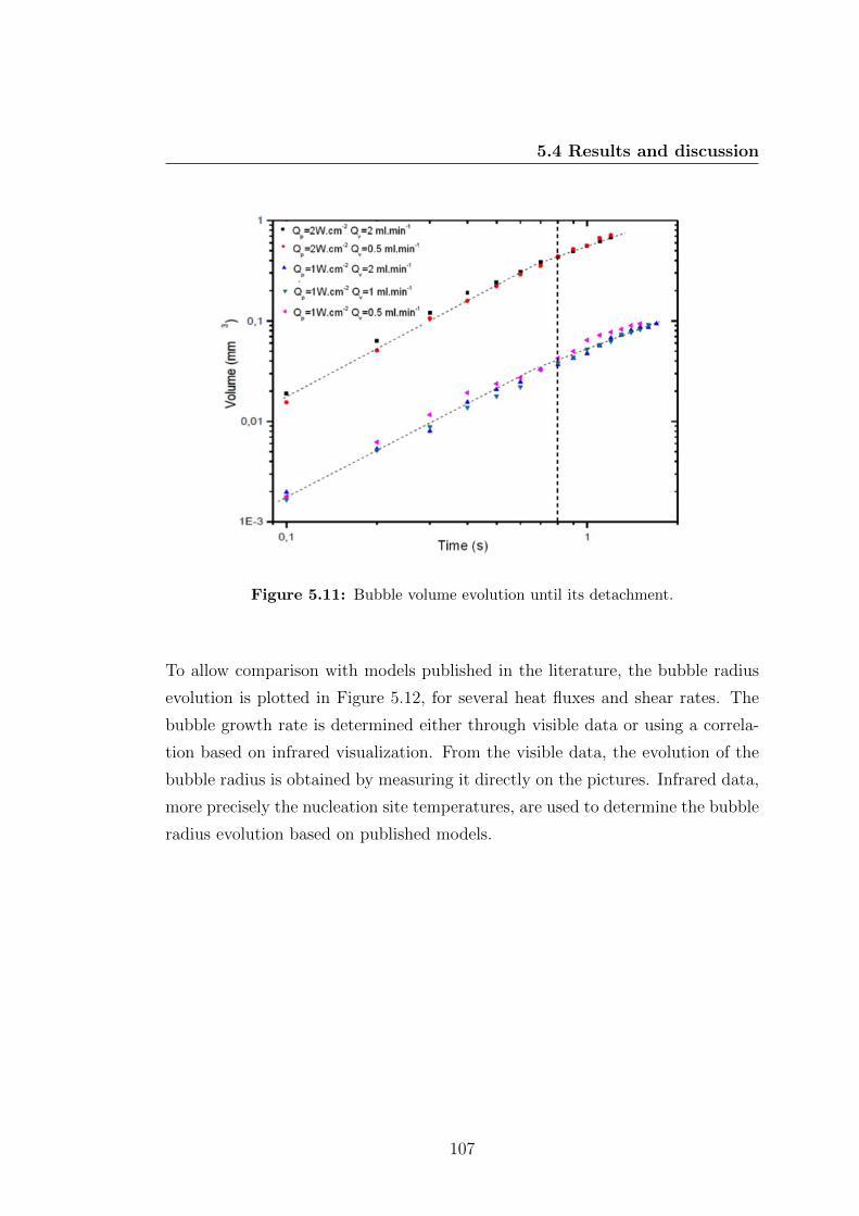
5.4 Results and discussion
Figure 5.11: Bubble volume evolution until its detachment.
To allow comparison with models published in the literature, the bubble radius
evolution is plotted in Figure 5.12, for several heat fluxes and shear rates. The
bubble growth rate is determined either through visible data or using a correla-
tion based on infrared visualization. From the visible data, the evolution of the
bubble radius is obtained by measuring it directly on the pictures. Infrared data,
more precisely the nucleation site temperatures, are used to determine the bubble
radius evolution based on published models.
107
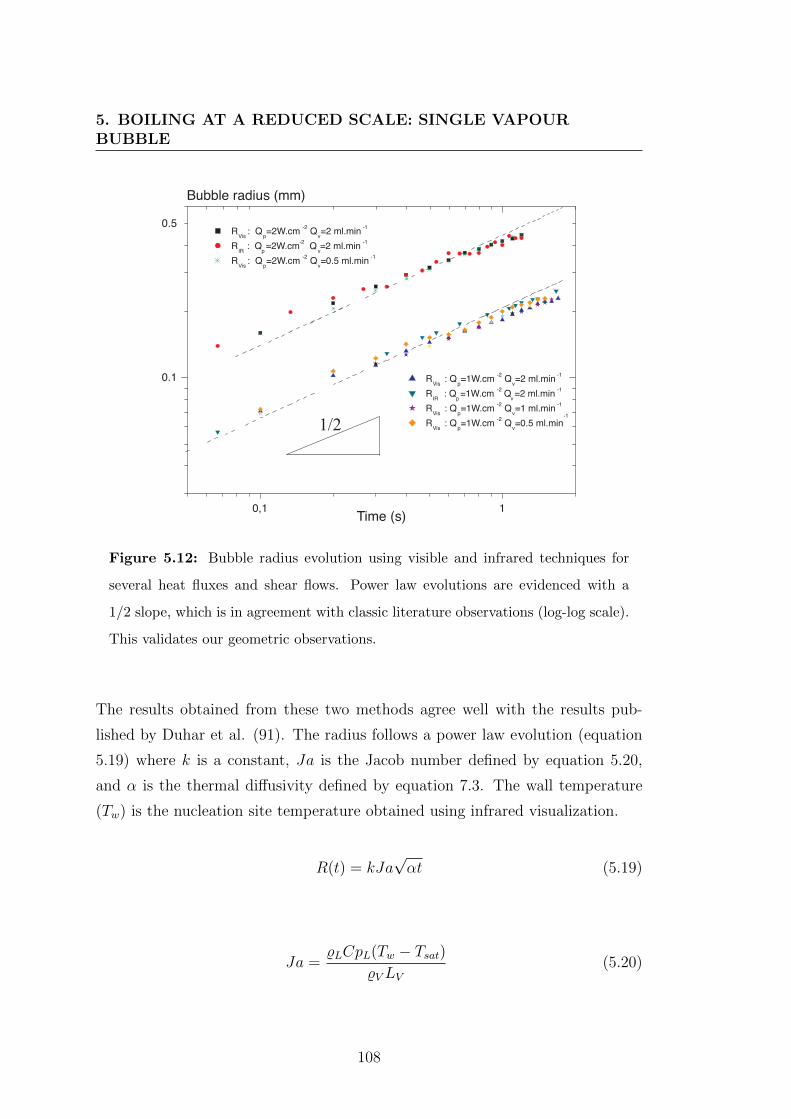
5. BOILING AT A REDUCED SCALE: SINGLE VAPOURBUBBLE
0,1 1
0.1
Bubble radius (mm)
Time (s)
RVis
: Qp=2W.cm
-2 Q
v=2 ml.min
-1
RIR
: Q p =2W.cm
-2 Q
v =2 ml.min
-1
RVis
: Qp=2W.cm
-2 Q
v=0.5 ml.min
-1
RVis
: Qp=1W.cm
-2 Q
v=2 ml.min
-1
RIR
: Q p =1W.cm
-2 Q
v =2 ml.min
-1
RVis
: Qp=1W.cm
-2 Q
v=1 ml.min
-1
RVis
: Qp=1W.cm
-2 Q
v=0.5 ml.min
-1
1/2
0.5
Figure 5.12: Bubble radius evolution using visible and infrared techniques for
several heat fluxes and shear flows. Power law evolutions are evidenced with a
1/2 slope, which is in agreement with classic literature observations (log-log scale).
This validates our geometric observations.
The results obtained from these two methods agree well with the results pub-
lished by Duhar et al. (91). The radius follows a power law evolution (equation
5.19) where k is a constant, Ja is the Jacob number defined by equation 5.20,
and α is the thermal diffusivity defined by equation 7.3. The wall temperature
(Tw) is the nucleation site temperature obtained using infrared visualization.
R(t) = kJa√αt (5.19)
Ja =%LCpL(Tw − Tsat)
%VLV(5.20)
108
5.4 Results and discussion
α =λ
%LCpL(5.21)
The value of k is not very sensitive to the fluid velocity or heat flux for this study
(k= 0.3 for all the heat fluxes and flow rates presented here). The experimen-
tal value of k can be compared to other models in literature based on different
assumptions. Cooper and Lloyd assumed that the bubble growth is mainly due
to the evaporation of the microlayer below the bubble base (76). They found a
value of k=2.5Pr−1/2, where Pr is the Prandtl number; for HFE-7000, k=0.89.
Other models based on evaporation on the whole bubble surface lead to a value
of k ranging between 1 and 2 (80). The experimental value obtained in this study
tends to show that the bubble growth is not only driven by the evaporation at
the triple line but possibly also along the liquid-vapour interface when the bubble
grows in shear flow.
5.4.1.3 Interface temperature and heat transfer
In regards to the bubble interface temperature homogeneity, the liquid-vapour
interface dynamic was observed from bubble nucleation until its detachment us-
ing infrared visualization. Figure 5.13 shows an image of a vapour bubble just
before its detachment from the nucleation site.
The shear flow is from right to left. The heating element is at the top of the test
cell. The exact position of the interface is underlined (dotted line) in an image
obtained from the visible light camera. Due to the calibration, the infrared im-
age enabled determination of the temperature field around the vapour bubble in
the liquid. Since the radiative heat flux arriving at the infrared camera detector
comes from the heated liquid, the data analysis is performed only in the liquid
part and at the bubble interface. Assuming a curved bubble interface in between
the two Hele-Shaw plates, the temperature coming from the interface is the one
coming from the liquid side. No quantitative data analysis is performed using
temperature coming from the inside of the bubble because that region is vapour
and has an undetermined emissivity.
109

5. BOILING AT A REDUCED SCALE: SINGLE VAPOURBUBBLE
Constant Heat Flux
Flow direction
37.9°C
37.1°C
0.5 mm
36.6°C
38
36
35
34
33
32
31
38.7°C
30.4°C
37
Figure 5.13: Infrared visualization of the bubble prior to departure from the
artificial nucleation site where a constant heat flux is applied. The liquid-vapour
interface (dotted line) is precisely located using the visible light camera. A sym-
metric bubble from a geometric point of view is observed; on the other hand, an
asymmetric bubble is observed in terms of interfacial temperature, with lower in-
terfacial temperature facing the flow.
From a geometric point of view, the vapour bubble remains perfectly axisym-
metric independent of the flow rate and heat flux. Since the mass flow rates are
relatively low, the bubble shape remains symmetric on both sides of the bubble
apex, upstream and downstream of the flow. However, Figure 5.13 shows that
just before bubble detachment, an asymmetric bubble interface temperature ex-
ists for specific conditions. It is nevertheless possible that such asymmetry may
not exist for all shear flows and heat fluxes, since two heat transfer mechanisms
are involved in convective boiling: viscous and convective forces.
110
5.4 Results and discussion
To evaluate the effects of both on the bubble interface temperature, the inter-
facial temperature was analyzed under a constant heat flux for different shear
flows. The competition between the two forces is compared using the Reynolds
number, which is based on the bubble diameter instead of the hydraulic diameter
in order to be related to the bubble itself without the test cell influence. Based
on this definition of the Reynolds number, the transitional Reynolds number will
not be dependent on the experimental configuration. Such a dimensionless value
is changed by varying the shear flow.
For the situations of Figure 5.14, the Reynolds number is varied between 0.58
and 2.34 and the bubble interface temperatures are plotted as a function of the
bubble curvilinear abscissa and for different stages of the bubble growth.The ori-
gin of the graph corresponds to the bubble apex.
While literature has only shown constant bubble interface temperatures far from
the triple line, Figure 5.14 provides experimental evidence that this interfacial
temperature is not constant and not always symmetric depending on the shear
flow.
For Reynolds numbers less than or equal to 0.82, a symmetric bubble interfacial
temperature exists on the bubble from its nucleation to its detachment as shown
in Figure 5.14 (a,b) in which five temperature profiles at different stages of the
growth are provided). For Reynolds numbers greater than or equal to 1.17 as
shown in Figure 5.14 (c,d), the bubble interfacial temperature is always asym-
metric from its nucleation to its detachment. These temperature differences along
the bubble interface cannot be neglected as they can reach values of 1.5C along
an interface of 0.8 mm in situations like those shown in Figure 5.14 (d).
In Figure 5.15, the degree of asymmetry is quantified. The highest difference is
the interfacial temperature profile for the different flow rates appears to be at the
final stage of the bubble growth. Figure 5.15 quantifies this degree of asymmetry
by comparing the temperature between each side of the bubble apex, at t=1.2s,
the final moment before the bubble detaches from the nucleation site. It appears
that below the critical value, there is no difference in the temperature profile
between each side of the bubble. It shows a symmetric temperature profile for
these low Reynolds numbers.
111

5. BOILING AT A REDUCED SCALE: SINGLE VAPOURBUBBLE
Inte
rfac
e Te
mpe
ratu
re (
°C)
-1000 -500 0 500 1000
36.0
36.5
37.0
37.5
38.0
38.5
39.0
Interface Length (µm)
t=1.2s
t=0.9s
t=0.7s
t=0.3s
t=0.1s
Flow direction
-1000 -500 0 500 1000
(a) (b)
(c) (d)36.0
36.5
37.0
37.5
38.0
38.5
39.0
36.0
36.5
37.0
37.5
38.0
38.5
39.0
36.0
36.5
37.0
37.5
38.0
38.5
39.0
Figure 5.14: Temperature along the bubble liquid-vapour interface for different
flow rates at different stages of bubble growth. Qp=2 W.cm−2; (a): Re=0.58, (b):
Re=0.82, (c): Re=1.17 and (d): Re=2.34.
Over the critical value of the Reynolds number, the difference in the temperature
from each side of the bubble increases along the bubble profile. It demonstrates
that the temperature profile becomes asymmetric over the critical value of the
Reynolds number.
112
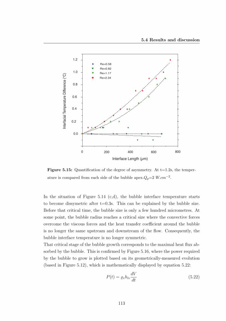
5.4 Results and discussion
0 400 800
Interface Length (µm)
Inte
rfac
ial T
empe
ratu
re D
iffer
ence
(°C
)
0.2
0.4
0.6
0.8
1.0
0.0
1.2
Re=0.58
Re=0.82
Re=2.34
Re=1.17
200 600
Figure 5.15: Quantification of the degree of asymmetry. At t=1.2s, the temper-
ature is compared from each side of the bubble apex.Qp=2 W.cm−2.
In the situation of Figure 5.14 (c,d), the bubble interface temperature starts
to become dissymetric after t=0.3s. This can be explained by the bubble size.
Before that critical time, the bubble size is only a few hundred micrometres. At
some point, the bubble radius reaches a critical size where the convective forces
overcome the viscous forces and the heat transfer coefficient around the bubble
is no longer the same upstream and downstream of the flow. Consequently, the
bubble interface temperature is no longer symmetric.
That critical stage of the bubble growth corresponds to the maximal heat flux ab-
sorbed by the bubble. This is confirmed by Figure 5.16, where the power required
by the bubble to grow is plotted based on its geometrically-measured evolution
(based in Figure 5.12), which is mathematically displayed by equation 5.22:
P (t) = %vhlvdV
dt(5.22)
113

5. BOILING AT A REDUCED SCALE: SINGLE VAPOURBUBBLE
In Figure 5.16, three power evolutions are plotted for different experimental con-
ditions (different heat fluxes and flow rates). All three curves show the same
dimensionless evolution. It is observed that the power absorbed by the bubble to
grow reaches a maximum at t∗ = 0.25 regardless of the inlet conditions. There is
a similar behaviour regardless of the flow rates and heat fluxes used. The max-
imum power absorbed by the bubble occurs at 25% of the bubble’s lifetime and
this time corresponds to the onset of thermal asymmetry of the bubble interface,
which was appearing after t=0.3s.
.
.
.
.
.
.
. . . . . .
Qp=2W.cm
-2 Q
v=2 ml.min
-1
Q p =2W.cm
-2 Q
v =0.5 ml.min
-1
Q =1W.cm-2
Q =2 ml.min-1
p v
Figure 5.16: Power required by a bubble to grow from nucleation to detachment.
P ∗ = PPmax
and t∗ = ttf
.
The comparison of the dimensionless number characterizing vapour bubble growth
in shear flow is presented in Table 5.1. It compares dimensionless numbers char-
acterizing the flow and the thermal, viscous and capillary effects, where Qv is the
114
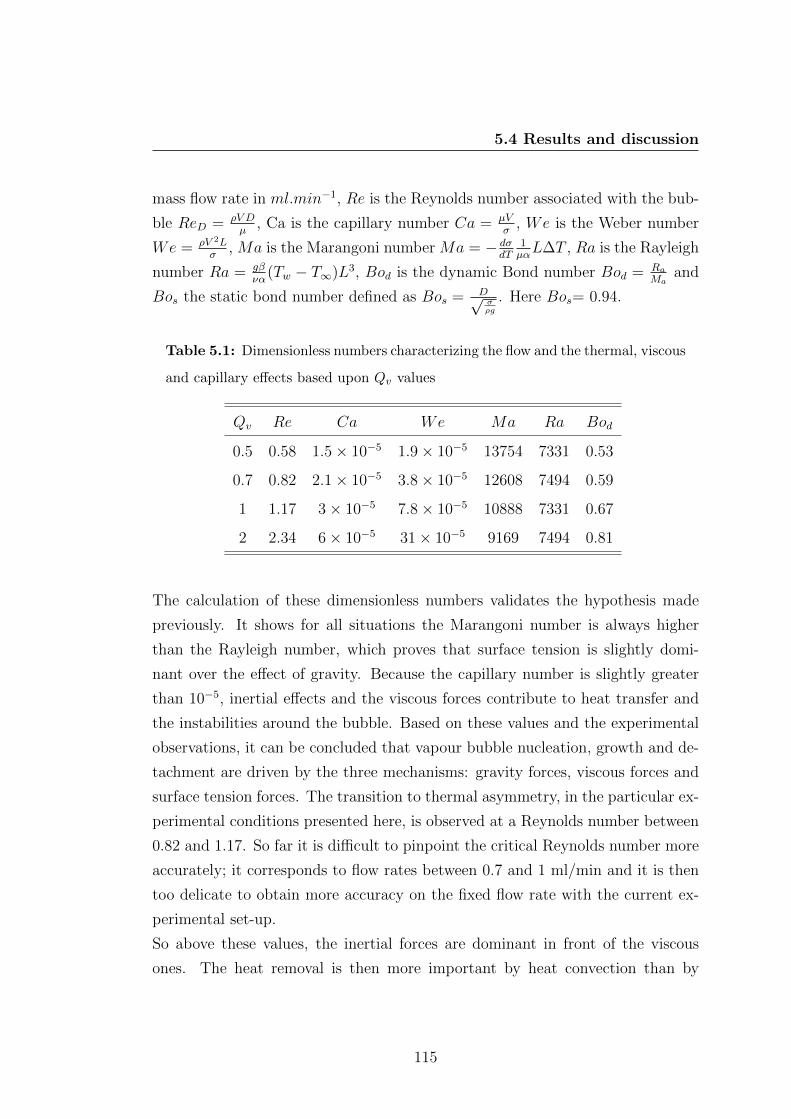
5.4 Results and discussion
mass flow rate in ml.min−1, Re is the Reynolds number associated with the bub-
ble ReD = ρV Dµ
, Ca is the capillary number Ca = µVσ
, We is the Weber number
We = ρV 2Lσ
, Ma is the Marangoni number Ma = − dσdT
1µαL∆T , Ra is the Rayleigh
number Ra = gβνα
(Tw − T∞)L3, Bod is the dynamic Bond number Bod = RaMa
and
Bos the static bond number defined as Bos = D√σρg
. Here Bos= 0.94.
Table 5.1: Dimensionless numbers characterizing the flow and the thermal, viscous
and capillary effects based upon Qv values
Qv Re Ca We Ma Ra Bod
0.5 0.58 1.5× 10⁻⁵ 1.9× 10⁻⁵ 13754 7331 0.53
0.7 0.82 2.1× 10⁻⁵ 3.8× 10⁻⁵ 12608 7494 0.59
1 1.17 3× 10⁻⁵ 7.8× 10⁻⁵ 10888 7331 0.67
2 2.34 6× 10⁻⁵ 31× 10−5 9169 7494 0.81
The calculation of these dimensionless numbers validates the hypothesis made
previously. It shows for all situations the Marangoni number is always higher
than the Rayleigh number, which proves that surface tension is slightly domi-
nant over the effect of gravity. Because the capillary number is slightly greater
than 10−5, inertial effects and the viscous forces contribute to heat transfer and
the instabilities around the bubble. Based on these values and the experimental
observations, it can be concluded that vapour bubble nucleation, growth and de-
tachment are driven by the three mechanisms: gravity forces, viscous forces and
surface tension forces. The transition to thermal asymmetry, in the particular ex-
perimental conditions presented here, is observed at a Reynolds number between
0.82 and 1.17. So far it is difficult to pinpoint the critical Reynolds number more
accurately; it corresponds to flow rates between 0.7 and 1 ml/min and it is then
too delicate to obtain more accuracy on the fixed flow rate with the current ex-
perimental set-up.
So above these values, the inertial forces are dominant in front of the viscous
ones. The heat removal is then more important by heat convection than by
115
5. BOILING AT A REDUCED SCALE: SINGLE VAPOURBUBBLE
viscous dissipation. Below these values, the viscous forces are dominating the
inertial ones. The bubble interface temperature is therefore more uniform due to
the low heat transfer removal by forced external convection. The assumption of
constant interfacial temperature is no longer justified. To obtain accurate results,
the bubble surface temperature variation has to be taken into account.
116

5.4 Results and discussion
5.4.2 Growth dynamic of nanofluids
This section presents the results for the bubble growth dynamic of nanofluids.
The results are comparing pure HFE7000 and HFE7000-Al2O3 at 1wt%. It was
shown in the previous paragraphs that the low flow rates used in this study
have minimal impact on the bubble growth dynamic. The results presented here
are for a fixed flow rate of 2 ml.min−1. The results for pure liquid, used as
comparison in this section, differ from those obtained in the previous paragraphs.
The experimental cell has been changed as well as the heating surface. However
the data presented here for pure liquid and the nanofluid were obtained with the
same experimental cell and heating element.
5.4.2.1 Thermal measurements
Nucleation site temperature
The infrared videos allow the observation of the vapour bubble growth cy-
cle, from its nucleation to its detachment and the changes in the nucleation site
temperature.
Figure 5.17 presents the temperature variation of the heating surface during the
growth of single vapour bubbles in pure liquid and HFE7000-Al2O3 at 1wt%,
for fixed heat fluxes of 3 W.cm−2 and 3.5 W.cm−2. The peaks followed by the
sharp decrease of the temperature correspond to the vapour bubble growth, where
energy is taken from the heating surface. The temperature of the surface then
increased after the detachment of the bubble to reach the temperature where the
next bubble will be created. The figure shows the maximum temperature reached
by pure liquid to be slightly higher than for the nanofluid. There is a difference of
approximately 0.5 K. Also, when the constant heat flux imposed on the heating
element is increased, the nucleation site temperature is logically increased. In
these particular conditions, for low heat flux, variation in the temperature dif-
ference between pure liquid and the nanofluid was not observed. For heat fluxes
ranging from 3 to 4 W.cm−2, the difference between pure liquid and the nanofluid
was measured to be approximately 0.5K.
117
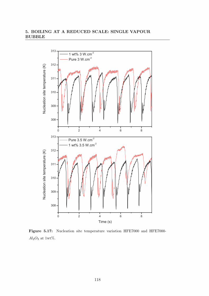
5. BOILING AT A REDUCED SCALE: SINGLE VAPOURBUBBLE
Figure 5.17: Nucleation site temperature variation HFE7000 and HFE7000-
Al2O3 at 1wt%.
118
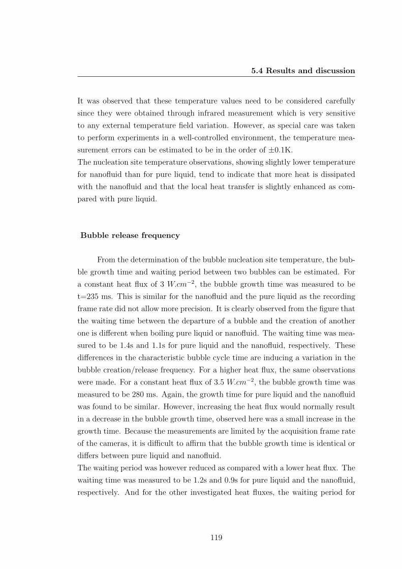
5.4 Results and discussion
It was observed that these temperature values need to be considered carefully
since they were obtained through infrared measurement which is very sensitive
to any external temperature field variation. However, as special care was taken
to perform experiments in a well-controlled environment, the temperature mea-
surement errors can be estimated to be in the order of ±0.1K.
The nucleation site temperature observations, showing slightly lower temperature
for nanofluid than for pure liquid, tend to indicate that more heat is dissipated
with the nanofluid and that the local heat transfer is slightly enhanced as com-
pared with pure liquid.
Bubble release frequency
From the determination of the bubble nucleation site temperature, the bub-
ble growth time and waiting period between two bubbles can be estimated. For
a constant heat flux of 3 W.cm−2, the bubble growth time was measured to be
t=235 ms. This is similar for the nanofluid and the pure liquid as the recording
frame rate did not allow more precision. It is clearly observed from the figure that
the waiting time between the departure of a bubble and the creation of another
one is different when boiling pure liquid or nanofluid. The waiting time was mea-
sured to be 1.4s and 1.1s for pure liquid and the nanofluid, respectively. These
differences in the characteristic bubble cycle time are inducing a variation in the
bubble creation/release frequency. For a higher heat flux, the same observations
were made. For a constant heat flux of 3.5 W.cm−2, the bubble growth time was
measured to be 280 ms. Again, the growth time for pure liquid and the nanofluid
was found to be similar. However, increasing the heat flux would normally result
in a decrease in the bubble growth time, observed here was a small increase in the
growth time. Because the measurements are limited by the acquisition frame rate
of the cameras, it is difficult to affirm that the bubble growth time is identical or
differs between pure liquid and nanofluid.
The waiting period was however reduced as compared with a lower heat flux. The
waiting time was measured to be 1.2s and 0.9s for pure liquid and the nanofluid,
respectively. And for the other investigated heat fluxes, the waiting period for
119

5. BOILING AT A REDUCED SCALE: SINGLE VAPOURBUBBLE
nanofluid was found to be lower than for pure liquid, inducing an increase in the
bubble release frequency. The calculation of the bubble release frequency based
on the bubble growth time and waiting period can be made with the following
equation:
f =1
τg + τwp(5.23)
where τg and τwp are the bubble growth time and the waiting period, respectively.
However, for more precision, to reduce measurement errors and to lower the im-
pact of the limited data acquisition frequency, the release frequency was obtained
by determining the number of nucleation, growth and detachment cycles over a
period of 20 seconds.
Figure 5.18 compares the bubble release frequency for pure HFE7000 and HFE7000-
Al2O3 at 1wt% for various heat fluxes (constant flow rate 2 ml.min−1). It shows,
as expected from the observations of the bubble growth time and waiting period,
that the frequency is higher for nanofluid than for pure liquid, and increases with
increasing the heat flux supplied to the heating surface. It was determined an
increase by 33% and 25% of the frequency for constant heat fluxes of 3 W.cm−2
and 3.5 W.cm−2, respectively, when using the nanofluid. The sharp increase in
the bubble frequency after 4 W.cm−2 is probably due to a change in the nucleate
boiling regime. It seems to correspond to the limit between partial and fully
nucleate boiling regime. Because of the infrared and visible camera limited ac-
quisition frequency, experiments at higher heat flux did not provide observable
and reliable data. Images were not clear enough to be treated, that is why the
presented results only focus on low heat fluxes.
120
5.4 Results and discussion
Figure 5.18: Bubble release frequency for HFE7000 and HFE7000-Al2O3 at
1wt%.
The determination of the nucleation site temperature and bubble release fre-
quency are giving results consistent with observations from the previous chapter
where the nanofluids were shown to increase the boiling performances. Actually,
the higher bubble departure frequency with nanofluid is consistent with the lower
wall temperature, since heat is removed more frequently.
121
5. BOILING AT A REDUCED SCALE: SINGLE VAPOURBUBBLE
5.4.2.2 Bubble growth dynamic
Bubble volume
The bubble geometrical characteristics, including the bubble maximum di-
ameter and height, were determined at each moment of the bubble growth by
simply measuring their values on the pictures. The values obtained were found
to be repeatable. From one bubble to another during a set of experiment, the
geometrical dimensions, as well as the surface temperature, were similar.
It is assumed that the vapour bubble is axisymmetric and has the shape of a
spherical cap. Since the maximum diameter reached by the bubble was observed
to be always smaller than the capillary length and the width of the experimental
cell, this assumption is reasonable. The bubble volume time variation was deter-
mined, based on the time variation of the maximum diameter and height of the
bubble.
Figure 5.19 shows a comparison between experimental results of time variation of
bubble volume for pure HFE 7000 and HFE7000-Al2O3 at 1wt% for two different
heat fluxes. The dependency of the volume with the heat flux is noticeable. The
bubble volume is increased with the increase of the wall heat flux. For a constant
heat flux, it appears that the bubble reaches a higher volume with pure liquid
than with the nanofluid. With increasing time, the volume variations between
pure liquid and nanofluid are increasing. At the beginning of the bubble growth
(time interval between 0 and approximately 50 ms), no or little variations are
observed between bubble volume evolution of pure liquid and nanofluid. After 50
ms, the volume becomes higher for pure liquid than for nanofluid. The changes in
the bubble volume evolution can be explained by two different growth stages. In
the early stage, growth is controlled by inertial effects similar for both nanofluid
and pure liquid. The changes in the bubble volume between pure liquid and the
nanofluid correspond to the moment when thermal diffusion and surface tension
effects become dominating. For the two heat fluxes presented here, the volume
variations when the bubble detaches from the nucleation surface reaches 18% and
28%. This smaller bubble volume at detachment is consistent with the observa-
tion of the bubble release frequency. Actually, an increase in the frequency will
122
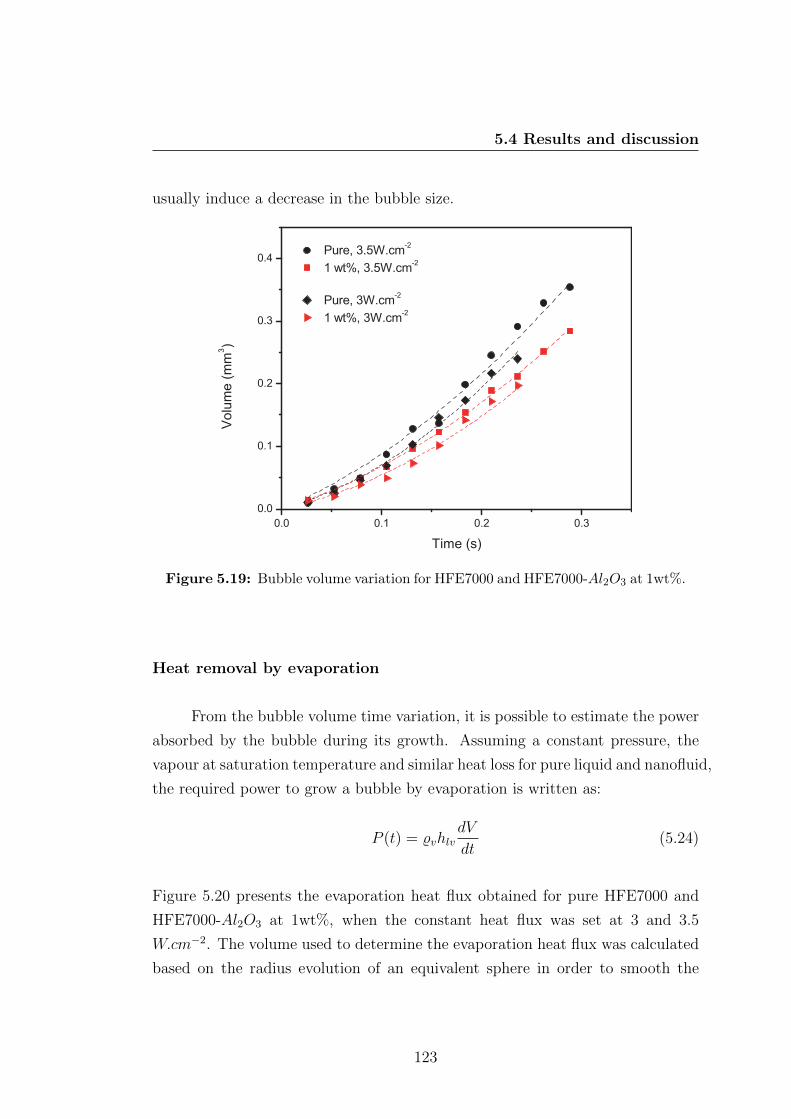
5.4 Results and discussion
usually induce a decrease in the bubble size.
Figure 5.19: Bubble volume variation for HFE7000 and HFE7000-Al2O3 at 1wt%.
Heat removal by evaporation
From the bubble volume time variation, it is possible to estimate the power
absorbed by the bubble during its growth. Assuming a constant pressure, the
vapour at saturation temperature and similar heat loss for pure liquid and nanofluid,
the required power to grow a bubble by evaporation is written as:
P (t) = %vhlvdV
dt(5.24)
Figure 5.20 presents the evaporation heat flux obtained for pure HFE7000 and
HFE7000-Al2O3 at 1wt%, when the constant heat flux was set at 3 and 3.5
W.cm−2. The volume used to determine the evaporation heat flux was calculated
based on the radius evolution of an equivalent sphere in order to smooth the
123

5. BOILING AT A REDUCED SCALE: SINGLE VAPOURBUBBLE
signal.
Figure 5.20: Power required to nucleate (P = 1bar,Qv = 2ml.min−1).
The evaporation power is increasing constantly as the bubble grows, which seems
logical as more and more vapour is required to increase the bubble size. The
power increases rapidly at the beginning of the growth and tends to stabilize. The
stabilization is probably due to condensation at the apex of the bubble after it
reaches a certain size. The difference between the pure liquid and nanofluid in the
evaporation heat flux was predictable. As for pure liquid, as the bubble reaches
a larger volume, it was expected that the evaporation heat flux would be higher.
However, the degree of variation is much bigger than for the bubble growth. An
approximation of the total power required to grow the bubble by evaporation can
be made by determining the area under the curves. For a constant heat flux of
3.5 W.cm−2, the total power by evaporation represents 31 and 26 mW , for pure
HFE7000 and HFE7000-Al2O3 at 1wt%, respectively. The power required for the
nanofluid is approximately 17% lower than for pure HFE7000. At 3 W.cm−2,
124
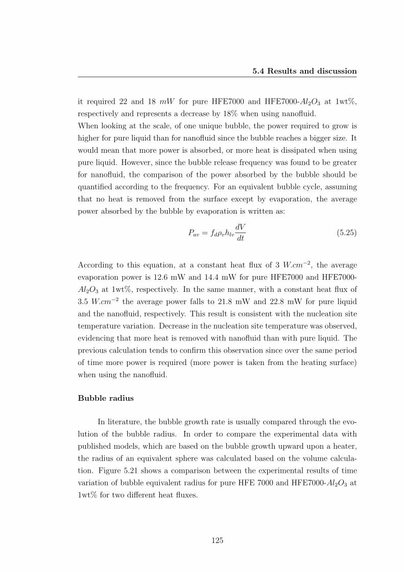
5.4 Results and discussion
it required 22 and 18 mW for pure HFE7000 and HFE7000-Al2O3 at 1wt%,
respectively and represents a decrease by 18% when using nanofluid.
When looking at the scale, of one unique bubble, the power required to grow is
higher for pure liquid than for nanofluid since the bubble reaches a bigger size. It
would mean that more power is absorbed, or more heat is dissipated when using
pure liquid. However, since the bubble release frequency was found to be greater
for nanofluid, the comparison of the power absorbed by the bubble should be
quantified according to the frequency. For an equivalent bubble cycle, assuming
that no heat is removed from the surface except by evaporation, the average
power absorbed by the bubble by evaporation is written as:
Pav = fdρvhlvdV
dt(5.25)
According to this equation, at a constant heat flux of 3 W.cm−2, the average
evaporation power is 12.6 mW and 14.4 mW for pure HFE7000 and HFE7000-
Al2O3 at 1wt%, respectively. In the same manner, with a constant heat flux of
3.5 W.cm−2 the average power falls to 21.8 mW and 22.8 mW for pure liquid
and the nanofluid, respectively. This result is consistent with the nucleation site
temperature variation. Decrease in the nucleation site temperature was observed,
evidencing that more heat is removed with nanofluid than with pure liquid. The
previous calculation tends to confirm this observation since over the same period
of time more power is required (more power is taken from the heating surface)
when using the nanofluid.
Bubble radius
In literature, the bubble growth rate is usually compared through the evo-
lution of the bubble radius. In order to compare the experimental data with
published models, which are based on the bubble growth upward upon a heater,
the radius of an equivalent sphere was calculated based on the volume calcula-
tion. Figure 5.21 shows a comparison between the experimental results of time
variation of bubble equivalent radius for pure HFE 7000 and HFE7000-Al2O3 at
1wt% for two different heat fluxes.
125
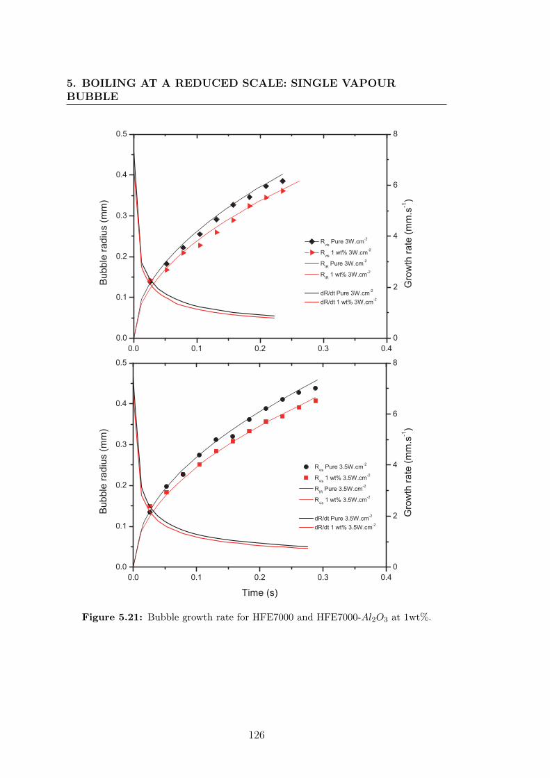
5. BOILING AT A REDUCED SCALE: SINGLE VAPOURBUBBLE
Figure 5.21: Bubble growth rate for HFE7000 and HFE7000-Al2O3 at 1wt%.
126
5.4 Results and discussion
In the same manner as for the volume evolution, at the beginning of the growth
very little variation is observed between pure liquid and the nanofluid. After 50
ms, the bubble radius of pure liquid becomes higher, as compared with the radius
with nanofluid. The variation tends to be higher with increased bubble growth
time. Higher bubble radii are observed for higher heat fluxes.
The dependency of the radius with time , as shown from the literature, is modeled
as follows:
R(t) = kJa√αt (5.26)
with
Ja =%LCpL(Tw − Tsat)
%VLV(5.27)
The Jacob number, Ja, was calculated with the infrared measurement of the
heating surface temperature. The coefficient k, was determined to be k=0.58 for
pure HFE7000, and k=0.6 for HFE7000-Al2O3 at 1wt% in order to fit to the
experimental data obtained via the geometric measurement of the radius. For
heat fluxes ranging between 3 and 4 W.cm−2, the values of k were found to be
identical. As shown in Figure 5.21, the vapour bubble radius evolutions deter-
mined either with the geometrical characteristics or with the thermal properties
and wall temperature are showing a good agreement after determination of the
constant, k.
This determination of the bubble radius evolution equation will allow a compari-
son with published models and help to determine what mechanisms could explain
the difference in the bubble growth of nanofluid as compared to pure liquid.
5.4.3 Bubble growth by evaporation of the microlayer
The results presented in the previous sections are consistent with an increase of
the heat transfer during boiling when using nanofluids. Actually, for the nanofluid
as compared with the base fluid, a decrease in the nucleation site temperature,
an increase in the bubble release frequency, smaller vapour bubbles and increase
in the heat removed by evaporation were observed. However, the challenge is
to explain these variations while remembering that the physical and thermal
127
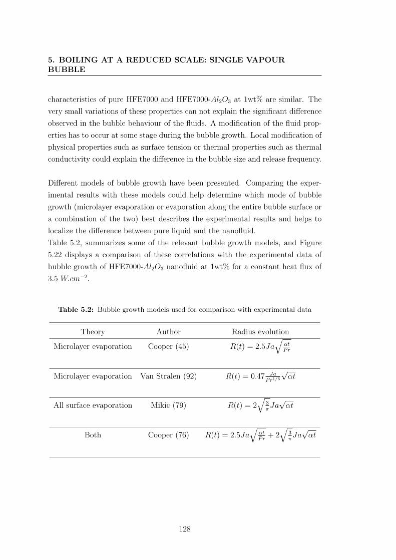
5. BOILING AT A REDUCED SCALE: SINGLE VAPOURBUBBLE
characteristics of pure HFE7000 and HFE7000-Al2O3 at 1wt% are similar. The
very small variations of these properties can not explain the significant difference
observed in the bubble behaviour of the fluids. A modification of the fluid prop-
erties has to occur at some stage during the bubble growth. Local modification of
physical properties such as surface tension or thermal properties such as thermal
conductivity could explain the difference in the bubble size and release frequency.
Different models of bubble growth have been presented. Comparing the exper-
imental results with these models could help determine which mode of bubble
growth (microlayer evaporation or evaporation along the entire bubble surface or
a combination of the two) best describes the experimental results and helps to
localize the difference between pure liquid and the nanofluid.
Table 5.2, summarizes some of the relevant bubble growth models, and Figure
5.22 displays a comparison of these correlations with the experimental data of
bubble growth of HFE7000-Al2O3 nanofluid at 1wt% for a constant heat flux of
3.5 W.cm−2.
Table 5.2: Bubble growth models used for comparison with experimental data
Theory Author Radius evolution
Microlayer evaporation Cooper (45) R(t) = 2.5Ja√
αtPr
Microlayer evaporation Van Stralen (92) R(t) = 0.47 JaPr1/6
√αt
All surface evaporation Mikic (79) R(t) = 2√
3πJa√αt
Both Cooper (76) R(t) = 2.5Ja√
αtPr
+ 2√
3πJa√αt
128
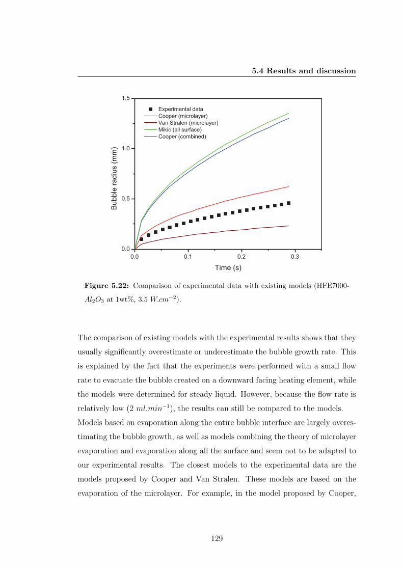
5.4 Results and discussion
Figure 5.22: Comparison of experimental data with existing models (HFE7000-
Al2O3 at 1wt%, 3.5 W.cm−2).
The comparison of existing models with the experimental results shows that they
usually significantly overestimate or underestimate the bubble growth rate. This
is explained by the fact that the experiments were performed with a small flow
rate to evacuate the bubble created on a downward facing heating element, while
the models were determined for steady liquid. However, because the flow rate is
relatively low (2 ml.min−1), the results can still be compared to the models.
Models based on evaporation along the entire bubble interface are largely overes-
timating the bubble growth, as well as models combining the theory of microlayer
evaporation and evaporation along all the surface and seem not to be adapted to
our experimental results. The closest models to the experimental data are the
models proposed by Cooper and Van Stralen. These models are based on the
evaporation of the microlayer. For example, in the model proposed by Cooper,
129
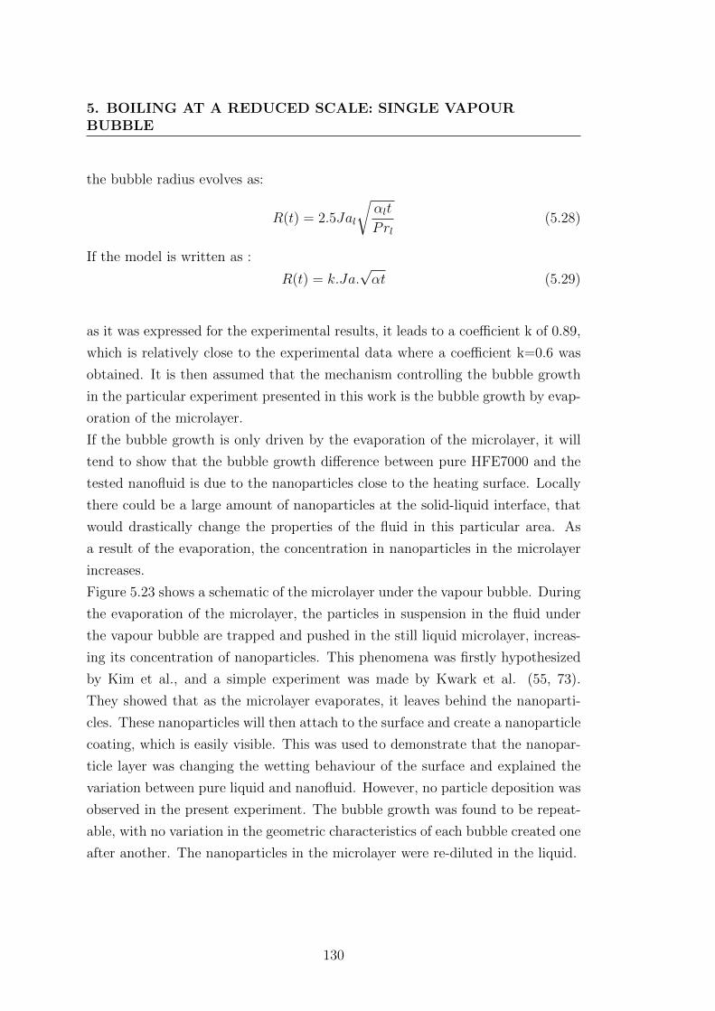
5. BOILING AT A REDUCED SCALE: SINGLE VAPOURBUBBLE
the bubble radius evolves as:
R(t) = 2.5Jal
√αlt
Prl(5.28)
If the model is written as :
R(t) = k.Ja.√αt (5.29)
as it was expressed for the experimental results, it leads to a coefficient k of 0.89,
which is relatively close to the experimental data where a coefficient k=0.6 was
obtained. It is then assumed that the mechanism controlling the bubble growth
in the particular experiment presented in this work is the bubble growth by evap-
oration of the microlayer.
If the bubble growth is only driven by the evaporation of the microlayer, it will
tend to show that the bubble growth difference between pure HFE7000 and the
tested nanofluid is due to the nanoparticles close to the heating surface. Locally
there could be a large amount of nanoparticles at the solid-liquid interface, that
would drastically change the properties of the fluid in this particular area. As
a result of the evaporation, the concentration in nanoparticles in the microlayer
increases.
Figure 5.23 shows a schematic of the microlayer under the vapour bubble. During
the evaporation of the microlayer, the particles in suspension in the fluid under
the vapour bubble are trapped and pushed in the still liquid microlayer, increas-
ing its concentration of nanoparticles. This phenomena was firstly hypothesized
by Kim et al., and a simple experiment was made by Kwark et al. (55, 73).
They showed that as the microlayer evaporates, it leaves behind the nanoparti-
cles. These nanoparticles will then attach to the surface and create a nanoparticle
coating, which is easily visible. This was used to demonstrate that the nanopar-
ticle layer was changing the wetting behaviour of the surface and explained the
variation between pure liquid and nanofluid. However, no particle deposition was
observed in the present experiment. The bubble growth was found to be repeat-
able, with no variation in the geometric characteristics of each bubble created one
after another. The nanoparticles in the microlayer were re-diluted in the liquid.
130

5.4 Results and discussion
Dry out area MicrolayerMicrolayer
Constant heat !ux
Vapor bubble
Microlayer
evaporation
Figure 5.23: Schematic of the microlayer under the vapour bubble.
With similar fluid properties, phenomena such as condensation at the bubble
apex, evaporation along the bubble surface or convection are assumed to be sim-
ilar for pure liquid and the nanofluid. The changes in the bubble behaviour then
rely on the drastic increase in the local physical and thermal properties modified
with the evaporation of the microlayer.
The determination of the microlayer evolution with time could lead to the deter-
mination of the concentration in nanoparticle in the microlayer and exhibit the
changes in the thermophysical properties in this area. Unfortunately, the exper-
imental set-up could not allow the determination of the microlayer size and its
evolution during bubble growth. Several methods exist to measure the microlayer
thickness such as laser interferometry as described by Koffman or using a laser
extinction method as explained by Utaka et al. (93, 94). With both of these
methods, a microlayer with thickness of a few micrometres was obtained, which
is too little to be measured with the current experimental apparatus. And an
estimation of the microlayer surface could be done by determining the dry-out
area left by the evaporating microlayer. A technical solution could be to position
an infrared camera above an infrared transparent heating surface as was done by
131
5. BOILING AT A REDUCED SCALE: SINGLE VAPOURBUBBLE
Schweitzer (95).
However, the local nanofluid concentration in the microlayer can be estimated
by determining the theoretical properties of the fluid that would explain the
difference in the bubble size between pure liquid and nanofluid. Normally, the
nanoparticle concentration would evolve with time and with the size of the mi-
crolayer. At the beginning of the growth, the concentration in nanoparticle is
that of the nanofluid everywhere else in the liquid (1wt%). During evaporation
of the microlayer, the concentration will theoretically range from 100wt% at the
triple line and 1wt% where the microlayer is in contact with the rest of the liq-
uid. The overall concentration will increase with the growth of the bubble and
the evaporation of the microlayer.
An average concentration in nanoparticles in the microlayer during the full bubble
growth, can be roughly estimated by determining the theoretical bubble growth
rate for different concentrations assuming that the vapour is only provided by the
evaporation of the microlayer. For this calculation, the micro layer is supposed
not to evolve with time. Based on the bubble growth model presented in the
previous paragraphs, the bubble growth dynamic with modified concentration
becomes:
R(t, φ) = kJa(φ)√α(φ)t (5.30)
with
Ja(φ) =%L(φ)CpL(φ)(Tw − Tsat)
%V (φ)hlv(5.31)
and
α =λ(φ)
%L(φ)CpL(φ)(5.32)
The values of thermal conductivity, specific heat capacity, liquid and vapour
density are determined according to the theoretical models presented in Chapter
3, hlv remains constant and the nucleation site temperature , Tw, is assumed to
be constant during the growth with different concentrations (shown to be untrue,
with a decrease by about 0.5K in the temperature with nanofluid as compared to
pure liquid).
132
5.4 Results and discussion
Figure 5.24 presents the bubble radius evolution for different nanoparticle con-
centrations in the microlayer and is compared to the experimental data obtained
for pure HFE7000 and HFE7000-Al2O3 at 1wt%.
Figure 5.24: Bubble radius evolution based on an increase of the nanoparticle
concentration in the microlayer.
It was shown that from the radius evolution obtained for pure liquid to the one
obtained with the nanofluid, the average concentration of nanoparticles should
increase to approximately 42wt%. This is an extreme difference as compared
to the actual concentration of the nanofluid. This value of nanoparticle concen-
tration represents only a very rough estimation since heavy assumptions were
made. The temperature of the nucleation site is not constant and appears to
be decreasing with the increase in the concentration. And the thermo-physical
properties were based on theoretical models. For example, the vapour density is
evolving in theory with the nanoparticle concentration while practically it will
remain close to the one of pure HFE7000. This estimation was mainly performed
to show that an increase in the microlayer properties might explain the bubble
133
5. BOILING AT A REDUCED SCALE: SINGLE VAPOURBUBBLE
growth difference between pure liquid and nanofluid. Also, in this comparison,
the bubble growth model is not taking into account the surface tension of the
fluid, that can also be modified, and will impact on bubble growth behaviour. It
will especially affect the bubble detachment. However, with such an increase of
the nanoparticle concentration, all the properties of the nanofluid are drastically
modified and this could explain the differences in the bubble growth dynamic,
both on a thermal and geometrical point of view.
The contribution of the thermo-physical properties, due to the increased concen-
tration of particles in the micro layer, will need to be investigated since they
can both affect the bubble behaviour. A time distribution of the nanofluid con-
centration in the microlayer could be calculated with the determination of the
microlayer dimension time variations.
5.5 Conclusions
The previous chapter showed that boiling heat transfer with nanofluid remains
contradictory and the need for a more fundamental approach to the boiling phe-
nomena at a more reduced scale was found. In the present chapter, boiling of
nanofluid was investigated at the scale of a single vapour bubble, in order to un-
derstand the possible mechanisms that induce the differences between the boiling
of a pure liquid or nanofluid. After a literature review focused on the bubble
nucleation, growth, and detachment cycle, where models describing the bubble
growth dynamic were presented, an experimental set-up based on a Hele-Shaw
cell was described. This configuration, where single vapour bubbles are created
on a unique nucleation site, allowed the observation of the growth dynamic from
the bubble nucleation to its detachment. The thermal and geometrical charac-
teristics of the growing bubbles were obtained via a set of visible and infrared
cameras. The results presented in this chapter, first, focus on the bubble growth
of pure liquid, with a particular emphasis on the liquid-vapour interface temper-
ature and are followed by a comparison of the bubble growth of pure HFE 7000
and HFE7000-Al2O3 nanofluid.
134
5.5 Conclusions
Experimental results for pure HFE 7000 show that the bubble interface temper-
ature far from the triple line is not constant. Furthermore, it was demonstrated
that in a situation of pool boiling, bubble growth is perfectly symmetric both
geometrically and thermally. However, for convective boiling, a critical bubble
Reynolds number, between 0.82 and 1.17, exists to distinguish two thermal sit-
uations. Below that threshold, the bubble grows symmetrically thermally, while
above, the bubble interface temperature exhibits a dissymmetric profile along
the interface. It was shown that this threshold corresponds to the moment in
which convective forces become dominant over viscous forces. In that regime, the
convective heat transfer facing the flow is no more the same as the heat trans-
fer behind the bubble. Consequently, in most of the situations encountered in
mechanical and chemical engineering applications, the constant interface temper-
ature assumption is not true and should taken into account the local heat transfer
removal effect. These results were published in Diana et al. (90).
The study of the bubble growth dynamic with nanofluids confirmed the results
obtained in the previous chapter, where an improvement of the heat transfer was
observed. As compared with the base fluid, boiling with nanofluid on a single
nucleation site exhibited an increase in the bubble release frequency (≈ 30%),
accompanied by a decrease in the bubble volume (≈ 25%). The nucleation site
temperature was therefore decreased with nanofluid by 0.5 K, evidencing a small
increase in the heat removed by evaporation. The little variations in the thermo-
physical properties of the nanofluid can not explain this behaviour. A theory
was then proposed, where the bubble growth is governed by the evaporation of
the microlayer, consisting of a thin liquid layer trapped under the vapour bub-
ble, evaporating with the bubble growing. It is proposed that the bubble growth
difference between pure liquid and nanofluid, is explained by a local drastic in-
crease in the thermo-physical properties of the liquid microlayer resulting from
its evaporation and an increase of the nanoparticle concentration.
One major objective for future work will be to characterize the local concentra-
tion in nanoparticle in the microlayer and determine the evolution of the local
fluid properties during the bubble growth.
135

5. BOILING AT A REDUCED SCALE: SINGLE VAPOURBUBBLE
136
6
Single vapour bubble in reduced
gravity
6.1 Introduction
In this chapter, results of the bubble growth with nanofluid in reduced gravity
are presented. A reason for performing experiments in a reduced gravity envi-
ronment relies upon the fact that most of the equations, models and correlations
describing the nucleate boiling process include gravity and buoyancy forces as the
dominant mechanism. In reduced gravity, buoyancy and natural convection are
significantly reduced and effects hidden in a normal gravity environment can be
revealed. In normal gravity, the bubble growth characteristics, including the de-
tachment diameter and bubble release frequency are described based on a bubble
force balance where buoyancy is the key mechanism.
A parameter not studied in the previous chapter was the influence of surface
tension on the bubble growth. In reduced gravity, this is expected to be a key
parameter in the mechanism of bubble growth and detachment. Other mecha-
nisms such as thermocapillary convection, or inertial effect could be revealed in
reduced gravity to provide some insights on the bubble growth with nanofluids.
The other justification for a reduced gravity experiment is driven by engineering
137
6. SINGLE VAPOUR BUBBLE IN REDUCED GRAVITY
demands. With the growing interest in space-based systems that would operate
without significant gravity forces present, the operating power requirements are
often high and thus heat transfer performance becomes more important. High
performance heat transfer systems are needed for applications such as electronic
component cooling, cryogenic fuel storage and transportation, propulsion or en-
ergy conversion systems and life support. As shown, for example, by Arlabosse
boiling heat transfer seems to be a very effective way in a reduced gravity en-
vironment (86). A clear understanding of the effect of gravity on the boiling
phenomena in reduced gravity is very important. If gravity effects on two-phase
systems can be quantified, the size and weight of these systems can be reduced,
reducing the launch cost of components, a major concern in current applications.
Nanofluids boiling shows promise in normal gravity, and experimental studies
in reduced gravity are a first step toward their implementation for space based
systems.
6.2 Literature review
The following section presents efforts that have been made for the understanding
of the boiling phenomena in reduced gravity. The first paragraph presents a
review of studies on the boiling heat transfer in reduced gravity. It is followed
by a presentation of some models of bubble growth characteristics, including
the bubble detachment diameter and release frequency, where gravity plays an
important role. No previous studies of nanofluid boiling in reduced gravity have
been made.
6.2.1 Boiling heat transfer in reduced gravity
Studies have been carried out to understand gravity effects that classical theories
and correlations do not properly predict. The correlation for nucleate boiling in
a pool by Rohsenow (equation 6.1) predicts that the heat flux should go to zero
in a reduced gravity environment but the experiments have shown this not to be
138

6.2 Literature review
true (41).
q = µlhlv
√g(ρl − ρv)
σ[Cpl(Tw − Tsat)
ChlvP nrl
]3 (6.1)
According to this correlation, the heat flux is supposed to approach zero in re-
duced gravity, but it has been shown that boiling heat transfer can be enhanced
or deteriorated or equalled in reduced gravity. An example is given by Stein-
bichler et al. who compared experimental results in normal gravity and reduced
gravity to the Roshenow’s correlation as shown in Figure 6.1 (6). They obtained
a 30% increase of the heat transfer coefficient while the correlation predicted a
reduction in the heat transfer coefficient by a factor of 100.
Figure 6.1: Comparison of experimental results and Roshenow’s correlation (6).
Many other correlations have been proposed over the past decades predicting
boiling phenomena from a heat transfer view as well as from the bubble dynamic
139

6. SINGLE VAPOUR BUBBLE IN REDUCED GRAVITY
view. However, even if good results are achieved in normal gravity, these corre-
lations do not properly characterize the boiling phenomena in a reduced gravity
environment. Excellent overviews of recent boiling heat transfer results were pro-
duced by Otha et al., Di Marco, Kim and Zhao (96, 97, 98, 99, 100).
Results concerning boiling in reduced gravity are controversial. Some studies
show enhancement of heat transfer in reduced gravity while others show deteri-
oration or negligible effect of gravity on heat transfer. Lui et al. reported an
increase in the heat transfer coefficient of up to 25 % when the gravity level was
reduced in nucleate boiling under subcooled liquid conditions (101). Lee and
Merte also observed enhancements in heat transfer of up to 32% while studying
boiling behaviour under a wide range of heat flux and subcoolings (102). Straub
et al. have been looking at boiling in reduced gravity since the early 1980s and
their results indicate that gravity has little effect on the overall heat transfer
(103, 104, 105). Otha et al. studied flow boiling of R113 in a vertical transparent
tube and show that the heat transfer was barely affected by gravity (106, 107).
As explained by Celata, reduced gravity conditions generally lead to a larger bub-
ble size (due to the absence of the buoyancy force) which is normally accompanied
by a deterioration in the heat transfer rate (108).
The previous research has shown that there is a lack of agreement on whether
heat transfer during boiling is enhanced or suppressed in reduced gravity. Re-
search still needs to be undertaken in order to obtain a full understanding of
boiling phenomena and especially the effect of gravity on boiling heat transfer.
However, to aid fundamental research, the reduced gravity environment is a very
interesting tool for the understanding of gravity hidden mechanisms that could
be responsible for bubble growth.
6.2.2 Bubble growth dynamic in reduced gravity
For studies in reduced gravity, relevant theoretical models and correlations de-
scribing the bubble growth dynamic include detachment diameter correlations
and bubble release frequency correlations, since most of these equations are re-
lated to gravity. Actually they usually relate to the Bond number, opposing the
gravitational forces to surface tension forces.
140
6.2 Literature review
6.2.2.1 Detachment diameter
There have been many correlations proposed for the predictions of the detachment
bubble diameter. Only a few are presented herein but a comprehensive review of
many models can be found in the work of Carey (4).
Many of these correlations include or are deviated from the Bond number (Eq.6.7)
which relates the gravitational forces to the surface tension (other forces might
be used sometimes):
Bo =g(ρl − ρv)D2
σ(6.2)
The first correlation was proposed by Fritz. It was assumed that there is a balance
between the surface tension and the buoyancy forces (42):
D = 0.0146θ
√2σ
g(ρl − ρv)(6.3)
However, many deviations were reported in the literature even if it allows the
determination of a correct length scale. This equation did not take into account
any thermal parameter or influence from the heating surface.
Zuber proposed a model that takes into account the effects of the wall super-
heat and the thermal boundary layer thickness (109):
D =
[σ
g(ρl − ρv)
] 13[
6λl(Tw − Tsat)q
] 13
(6.4)
A simple model was proposed by Cole including the surface temperature effect
with the Jakob number (110):
D = 0.04Ja
√2σ
g(ρl − ρv)(6.5)
and was improved later by Cole and Rohsenow by replacing the wall temperature
with the critical temperature, since their experimental results showed that the
141
6. SINGLE VAPOUR BUBBLE IN REDUCED GRAVITY
bubble diameter was proportional to the critical temperature rather than to the
wall temperature (111). In their equation, a coefficient is proposed depending on
the investigated fluid:
D = CJa54
√σg0
g(ρl − ρv)(6.6)
with C = 1.5× 10⁻⁴ for water and C = 4.65× 10⁻⁴ for other liquids.
Van Stralen later proposed an empirical model for the detachment diameter in
nucleate boiling considering the thermal diffusivity and the Jakob number (112):
D = 2.63
[Ja2α2
l
g
) 13
[1 +
(2π
3Ja
) 12
] 14
(6.7)
Another model taking into account the thermal properties and the effect of the
wall superheat was proposed by Kutateladze and Gogonin (113):
D =[0.25(1 + 105K1)1/2
]( σ
g(ρl − ρv)
)1/2
(6.8)
where,
K1 =
(ρlCpl(Tw − Tsat)
ρvhlvPr
)2[µ2l [g(ρl − ρv)]1/2
ρlσ3/2
](6.9)
Based on the previous model, Jensen and Memmel, proposed a model that was
predicting the detachment diameter with an higher accuracy when comparing
with an extensive data base (114):
D =[0.19(1.8 + 105K1)1/2
]( σ
g(ρl − ρv)
)1/2
(6.10)
In most cases, the bubble shape is not spherical. The departure diameter in
most of these models corresponds to the detachment diameter of an equivalent
sphere with a volume equal to the volume of the considered bubble. In all these
models, the dependence of the detachment diameter on gravity is evident and has
been reported experimentally.
142
6.2 Literature review
6.2.2.2 Departure frequency
Nucleate boiling phenomena are also characterized by the bubble release fre-
quency, which is determined as the inverse sum of the bubble growth time and
waiting time. It appears that the bubble release frequency is dependent on the
bubble detachment diameter since the bubble growth rate and the bubble size
are required to determine the characteristic times, then the bubble departure
frequency. Most of the significant correlations for the bubble frequency, fb, have
been summarized by Carey. The following paragraph presents some of the main
ones (4).
The first model presented by Jakob and Fritz, proposed a simple relationship
between the detachment diameter and release frequency as (115):
fd.Dd = 0.078 (6.11)
Zuber later proposed a model based on an analogy between bubble detachment
and natural convection (116):
fd.Dd = 0.59
[σg(ρl − ρv)
ρ2l
] 14
(6.12)
Malenkov used the detachment diameter proposed by Fritz to develop his model
taking into account various parameters (117):
fd =Va
Ddπ(
1− 11+Vaρvδhv/q
) (6.13)
where
Va =
√Ddg(ρl − ρv)
2(ρl + ρv)+
2σ
D(ρl + ρv)(6.14)
The model proposed by Mikic and Rohsenhow derived their own model of bubble
growth (presented in Chapter 4) and obtained (118):
143
6. SINGLE VAPOUR BUBBLE IN REDUCED GRAVITY
fdDd =4
πJa√
3πα
[(τg
τwt + τg
)1/2
+
(1 +
τgτwt + τg
)1/2
− 1
](6.15)
The growth time and waiting time being usually hard to determine or unknown,
they simplified their model as:
f1/2d .Dd = 0.83Ja
√πα (6.16)
when 0.15 < τwtτwt+τg
< 0.8.
Finally, for Ivey, the relations between the frequency and diameter depend on
what mechanisms control the bubble growth and give (119):
• Hydrodynamic phase: f 2d .Dd = const, for inertia controlled bubble growth.
• Thermodynamic phase: f1/2d .Dd = const, for heat transfer controlled bubble
growth.
• Transition: fnd .Dd = const, when both mechanisms are involved in the
detachment process, 12< n < 2.
144
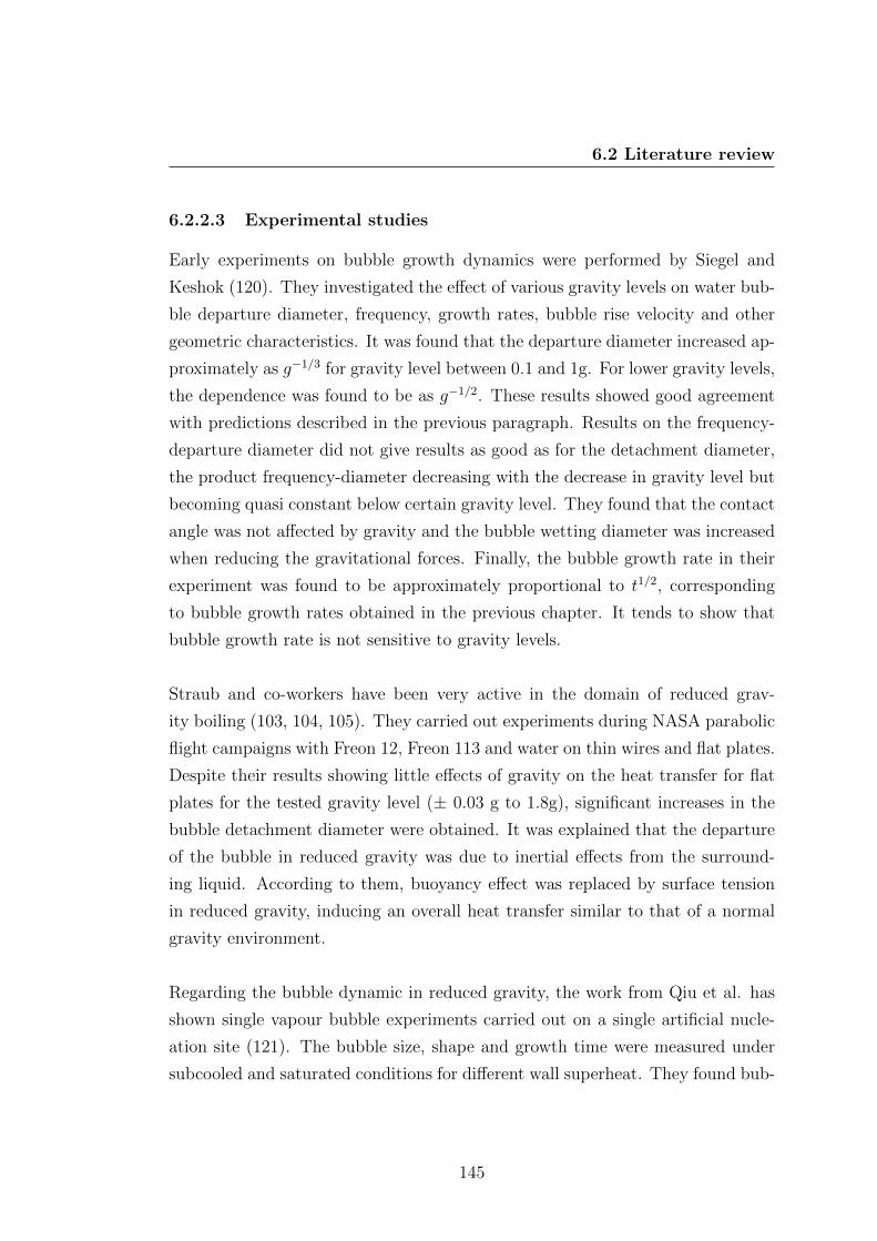
6.2 Literature review
6.2.2.3 Experimental studies
Early experiments on bubble growth dynamics were performed by Siegel and
Keshok (120). They investigated the effect of various gravity levels on water bub-
ble departure diameter, frequency, growth rates, bubble rise velocity and other
geometric characteristics. It was found that the departure diameter increased ap-
proximately as g−1/3 for gravity level between 0.1 and 1g. For lower gravity levels,
the dependence was found to be as g−1/2. These results showed good agreement
with predictions described in the previous paragraph. Results on the frequency-
departure diameter did not give results as good as for the detachment diameter,
the product frequency-diameter decreasing with the decrease in gravity level but
becoming quasi constant below certain gravity level. They found that the contact
angle was not affected by gravity and the bubble wetting diameter was increased
when reducing the gravitational forces. Finally, the bubble growth rate in their
experiment was found to be approximately proportional to t1/2, corresponding
to bubble growth rates obtained in the previous chapter. It tends to show that
bubble growth rate is not sensitive to gravity levels.
Straub and co-workers have been very active in the domain of reduced grav-
ity boiling (103, 104, 105). They carried out experiments during NASA parabolic
flight campaigns with Freon 12, Freon 113 and water on thin wires and flat plates.
Despite their results showing little effects of gravity on the heat transfer for flat
plates for the tested gravity level (± 0.03 g to 1.8g), significant increases in the
bubble detachment diameter were obtained. It was explained that the departure
of the bubble in reduced gravity was due to inertial effects from the surround-
ing liquid. According to them, buoyancy effect was replaced by surface tension
in reduced gravity, inducing an overall heat transfer similar to that of a normal
gravity environment.
Regarding the bubble dynamic in reduced gravity, the work from Qiu et al. has
shown single vapour bubble experiments carried out on a single artificial nucle-
ation site (121). The bubble size, shape and growth time were measured under
subcooled and saturated conditions for different wall superheat. They found bub-
145

6. SINGLE VAPOUR BUBBLE IN REDUCED GRAVITY
ble size to be significantly higher, with longer growth period in reduced gravity
as compared to results in a normal gravity environment. For identical experi-
mental conditions, including wall superheat and subcooling level, they found a
dependency of the bubble growth time and detachment diameter with gravity as:
Dd ≈ g−0.5 and tg ≈ g−0.5, which was consistent with several models published in
the literature.
Serret et al. studied the influence of reduced gravity on the bubble growth and
detachment of pure HFE-7100 in an experimental cell similar to the one used in
this work (88). The heating is also facing downward and the parameters investi-
gated included various shear flows and heat fluxes. It was found that with this
configuration, the bubble detachment diameter and the bubble growth time was
decreased in reduced gravity, as compared with normal gravity. They found that
reduced gravity increases the nucleation frequency and obtained higher variation
of the nucleation site temperature, which, in this case, tends to demonstrate an
increase in the local heat transfer coefficient. The differences with previous work,
where the bubble size was increased in normal gravity is explained by the special
configuration of the heater which was chosen to obtain observable higher bubble
size in normal gravity and allows comparison with reduced gravity results.
146
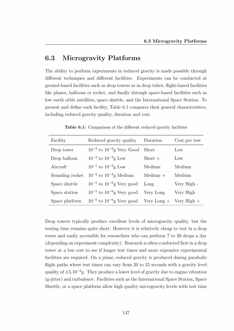
6.3 Microgravity Platforms
6.3 Microgravity Platforms
The ability to perform experiments in reduced gravity is made possible through
different techniques and different facilities. Experiments can be conducted at
ground-based facilities such as drop towers or in drop tubes, flight-based facilities
like planes, balloons or rocket, and finally through space-based facilities such as
low earth orbit satellites, space shuttle, and the International Space Station. To
present and define each facility, Table 6.1 compares their general characteristics,
including reduced gravity quality, duration and cost.
Table 6.1: Comparison of the different reduced gravity facilities
Facility Reduced gravity quality Duration Cost per test
Drop tower 10−2 to 10−6g Very Good Short Low
Drop balloon 10−2 to 10−3g Low Short + Low
Aircraft 10−1 to 10−3g Low Medium Medium
Sounding rocket 10−2 to 10−4g Medium Medium + Medium
Space shuttle 10−5 to 10−6g Very good Long Very High -
Space station 10−5 to 10−6g Very good Very Long Very High
Space platform 10−5 to 10−6g Very good Very Long + Very High +
Drop towers typically produce excellent levels of microgravity quality, but the
testing time remains quite short. However it is relatively cheap to test in a drop
tower and easily accessible for researchers who can perform 7 to 20 drops a day
(depending on experiment complexity). Research is often conducted first in a drop
tower at a low cost to see if longer test times and more expensive experimental
facilities are required. On a plane, reduced gravity is produced during parabolic
flight paths where test times can vary from 20 to 25 seconds with a gravity level
quality of ±5.10−2g. They produce a lower level of gravity due to engine vibration
(g-jitter) and turbulence. Facilities such as the International Space Station, Space
Shuttle, or a space platform allow high quality microgravity levels with test time
147
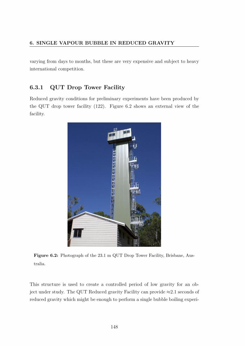
6. SINGLE VAPOUR BUBBLE IN REDUCED GRAVITY
varying from days to months, but these are very expensive and subject to heavy
international competition.
6.3.1 QUT Drop Tower Facility
Reduced gravity conditions for preliminary experiments have been produced by
the QUT drop tower facility (122). Figure 6.2 shows an external view of the
facility.
Figure 6.2: Photograph of the 23.1 m QUT Drop Tower Facility, Brisbane, Aus-
tralia.
This structure is used to create a controlled period of low gravity for an ob-
ject under study. The QUT Reduced gravity Facility can provide ≈2.1 seconds of
reduced gravity which might be enough to perform a single bubble boiling experi-
148
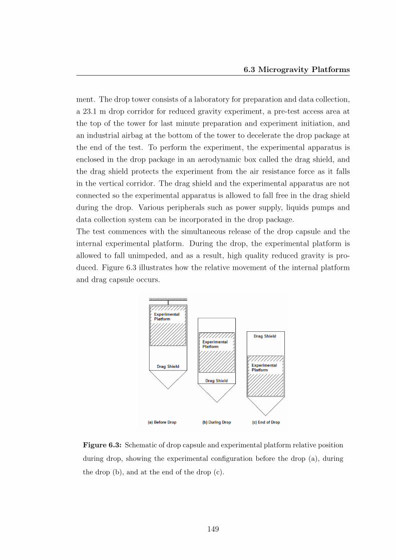
6.3 Microgravity Platforms
ment. The drop tower consists of a laboratory for preparation and data collection,
a 23.1 m drop corridor for reduced gravity experiment, a pre-test access area at
the top of the tower for last minute preparation and experiment initiation, and
an industrial airbag at the bottom of the tower to decelerate the drop package at
the end of the test. To perform the experiment, the experimental apparatus is
enclosed in the drop package in an aerodynamic box called the drag shield, and
the drag shield protects the experiment from the air resistance force as it falls
in the vertical corridor. The drag shield and the experimental apparatus are not
connected so the experimental apparatus is allowed to fall free in the drag shield
during the drop. Various peripherals such as power supply, liquids pumps and
data collection system can be incorporated in the drop package.
The test commences with the simultaneous release of the drop capsule and the
internal experimental platform. During the drop, the experimental platform is
allowed to fall unimpeded, and as a result, high quality reduced gravity is pro-
duced. Figure 6.3 illustrates how the relative movement of the internal platform
and drag capsule occurs.
Figure 6.3: Schematic of drop capsule and experimental platform relative position
during drop, showing the experimental configuration before the drop (a), during
the drop (b), and at the end of the drop (c).
149
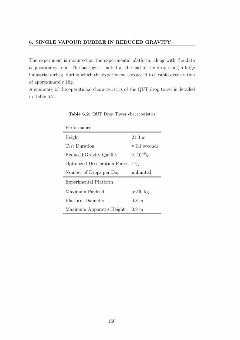
6. SINGLE VAPOUR BUBBLE IN REDUCED GRAVITY
The experiment is mounted on the experimental platform, along with the data
acquisition system. The package is halted at the end of the drop using a large
industrial airbag, during which the experiment is exposed to a rapid deceleration
of approximately 18g.
A summary of the operational characteristics of the QUT drop tower is detailed
in Table 6.2.
Table 6.2: QUT Drop Tower characteristics
Performance
Height 21.3 m
Test Duration ≈2.1 seconds
Reduced Gravity Quality < 10−6g
Optimized Deceleration Force 17g
Number of Drops per Day unlimited
Experimental Platform
Maximum Payload ≈200 kg
Platform Diameter 0.8 m
Maximum Apparatus Height 0.9 m
150
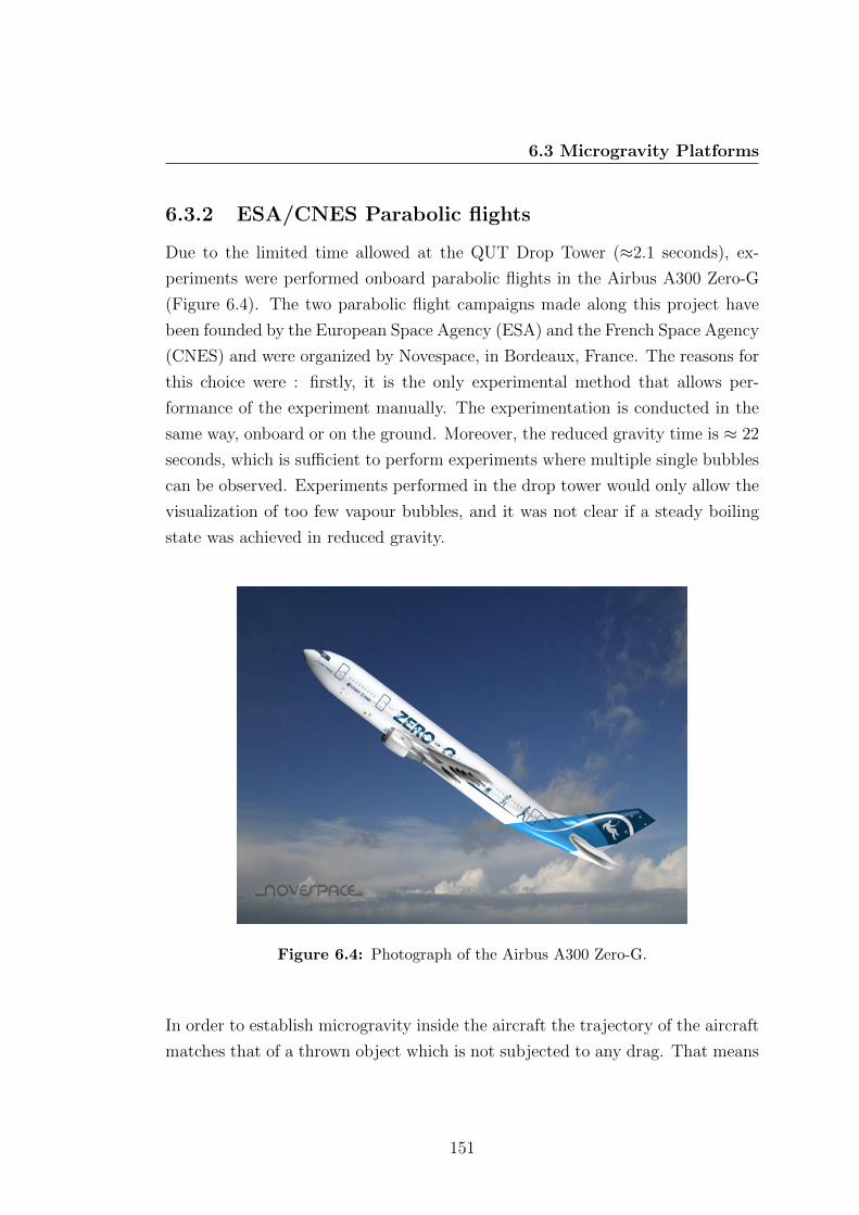
6.3 Microgravity Platforms
6.3.2 ESA/CNES Parabolic flights
Due to the limited time allowed at the QUT Drop Tower (≈2.1 seconds), ex-
periments were performed onboard parabolic flights in the Airbus A300 Zero-G
(Figure 6.4). The two parabolic flight campaigns made along this project have
been founded by the European Space Agency (ESA) and the French Space Agency
(CNES) and were organized by Novespace, in Bordeaux, France. The reasons for
this choice were : firstly, it is the only experimental method that allows per-
formance of the experiment manually. The experimentation is conducted in the
same way, onboard or on the ground. Moreover, the reduced gravity time is ≈ 22
seconds, which is sufficient to perform experiments where multiple single bubbles
can be observed. Experiments performed in the drop tower would only allow the
visualization of too few vapour bubbles, and it was not clear if a steady boiling
state was achieved in reduced gravity.
Figure 6.4: Photograph of the Airbus A300 Zero-G.
In order to establish microgravity inside the aircraft the trajectory of the aircraft
matches that of a thrown object which is not subjected to any drag. That means
151
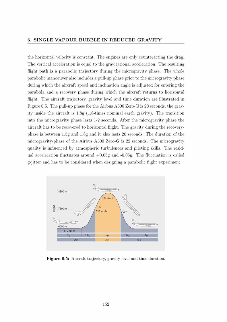
6. SINGLE VAPOUR BUBBLE IN REDUCED GRAVITY
the horizontal velocity is constant. The engines are only counteracting the drag.
The vertical acceleration is equal to the gravitational acceleration. The resulting
flight path is a parabolic trajectory during the microgravity phase. The whole
parabolic manoeuver also includes a pull-up phase prior to the microgravity phase
during which the aircraft speed and inclination angle is adjusted for entering the
parabola and a recovery phase during which the aircraft returns to horizontal
flight. The aircraft trajectory, gravity level and time duration are illustrated in
Figure 6.5. The pull-up phase for the Airbus A300 Zero-G is 20 seconds, the grav-
ity inside the aircraft is 1.8g (1.8-times nominal earth gravity). The transition
into the microgravity phase lasts 1-2 seconds. After the microgravity phase the
aircraft has to be recovered to horizontal flight. The gravity during the recovery-
phase is between 1.5g and 1.8g and it also lasts 20 seconds. The duration of the
microgravity-phase of the Airbus A300 Zero-G is 22 seconds. The microgravity
quality is influenced by atmospheric turbulences and piloting skills. The resid-
ual acceleration fluctuates around +0.05g and -0.05g. The fluctuation is called
g-jitter and has to be considered when designing a parabolic flight experiment.
Figure 6.5: Aircraft trajectory, gravity level and time duration.
152

6.3 Microgravity Platforms
For the design of a parabolic flight experiment the safety rules and guidelines
of the aircraft operating company have to be fulfilled. That makes a parabolic
flight experiment much more complex compared to a similar ground experiment.
Additionally, special precautions regarding the reliability of the experiment have
to be taken since it is not possible to perform any reparation during the flight.
Only small modifications can be carried out in between the flights which take
place on successive days.
The parabolic flight campaigns of ESA, DLR and CNES take place at Bordeaux
Merignac airport where the Airbus A300 zero-g is sited. Roughly 14 to 16 exper-
iments take part in one campaign. The campaign lasts 10 to 11 days. The first
week is used for experiment preparation. The experiments are set up from trans-
port to flight configuration. All experiments have to pass a preliminary safety
review before they are allowed to be loaded into the aircraft. The second week is
the flight week. An official safety review is again performed by the French test
flight centre CEV prior to flights day. Over the next three days, the parabolic
flights with 31 parabolas in each flight are performed, with an average of three
hours per flight.
The parabolas are flown in intervals of 3 min with some minutes break after sets
of 5 parabolas. This also has to be taken into account during the experiment
planning. Experimental data has to be stored and the next run has to be pre-
pared within these 2 min. In the present case, this time was the limiting factor
for the number of high speed camera images. The images had to be transferred
from the camera to the computer and stored onto hard disc.
153
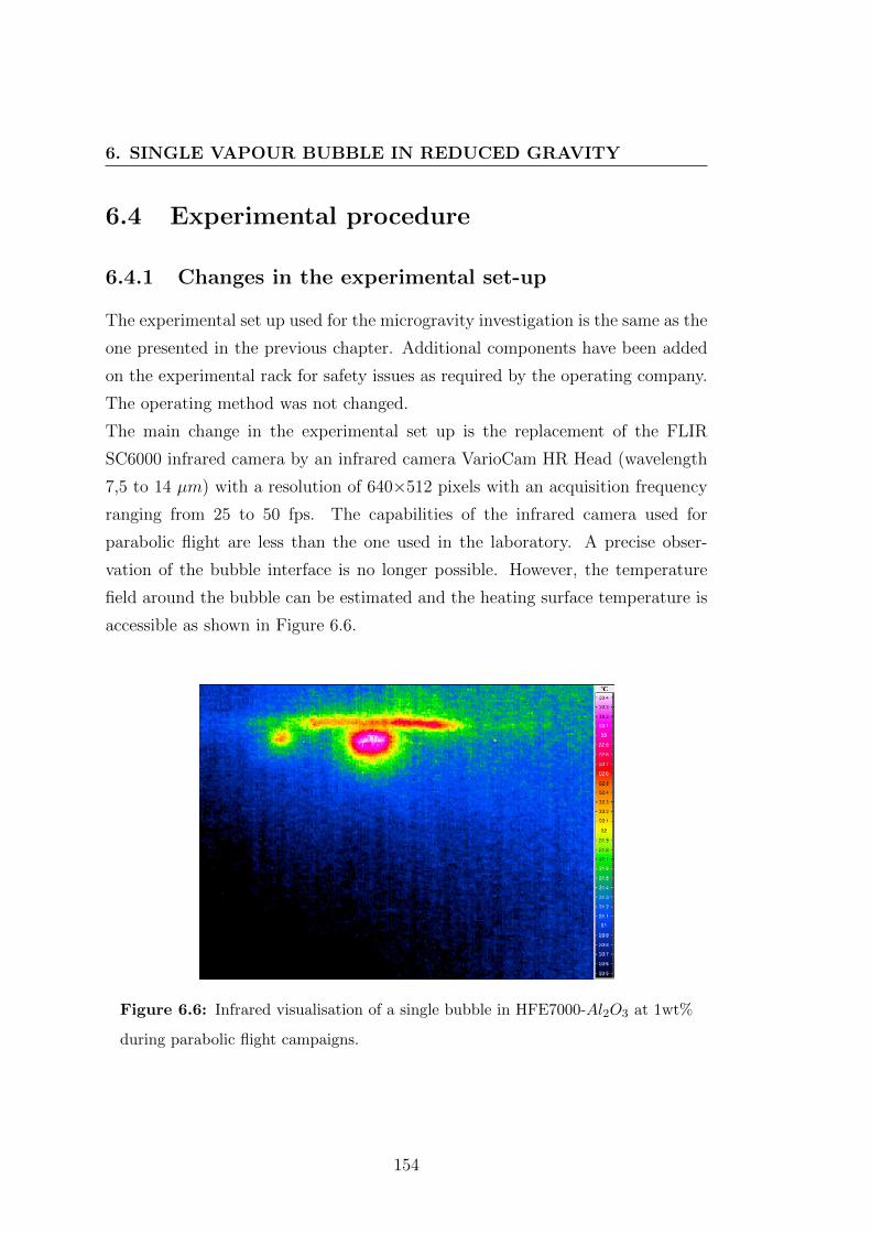
6. SINGLE VAPOUR BUBBLE IN REDUCED GRAVITY
6.4 Experimental procedure
6.4.1 Changes in the experimental set-up
The experimental set up used for the microgravity investigation is the same as the
one presented in the previous chapter. Additional components have been added
on the experimental rack for safety issues as required by the operating company.
The operating method was not changed.
The main change in the experimental set up is the replacement of the FLIR
SC6000 infrared camera by an infrared camera VarioCam HR Head (wavelength
7,5 to 14 µm) with a resolution of 640×512 pixels with an acquisition frequency
ranging from 25 to 50 fps. The capabilities of the infrared camera used for
parabolic flight are less than the one used in the laboratory. A precise obser-
vation of the bubble interface is no longer possible. However, the temperature
field around the bubble can be estimated and the heating surface temperature is
accessible as shown in Figure 6.6.
Figure 6.6: Infrared visualisation of a single bubble in HFE7000-Al2O3 at 1wt%
during parabolic flight campaigns.
154
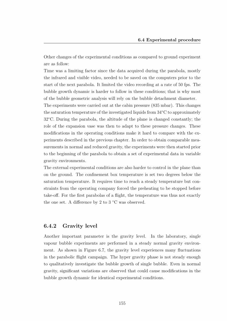
6.4 Experimental procedure
Other changes of the experimental conditions as compared to ground experiment
are as follow:
Time was a limiting factor since the data acquired during the parabola, mostly
the infrared and visible video, needed to be saved on the computers prior to the
start of the next parabola. It limited the video recording at a rate of 50 fps. The
bubble growth dynamic is harder to follow in these conditions; that is why most
of the bubble geometric analysis will rely on the bubble detachment diameter.
The experiments were carried out at the cabin pressure (835 mbar). This changes
the saturation temperature of the investigated liquids from 34C to approximately
32C. During the parabola, the altitude of the plane is changed constantly; the
role of the expansion vase was then to adapt to these pressure changes. These
modifications in the operating conditions make it hard to compare with the ex-
periments described in the previous chapter. In order to obtain comparable mea-
surements in normal and reduced gravity, the experiments were then started prior
to the beginning of the parabola to obtain a set of experimental data in variable
gravity environments.
The external experimental conditions are also harder to control in the plane than
on the ground. The confinement box temperature is set two degrees below the
saturation temperature. It requires time to reach a steady temperature but con-
straints from the operating company forced the preheating to be stopped before
take-off. For the first parabolas of a flight, the temperature was thus not exactly
the one set. A difference by 2 to 3 C was observed.
6.4.2 Gravity level
Another important parameter is the gravity level. In the laboratory, single
vapour bubble experiments are performed in a steady normal gravity environ-
ment. As shown in Figure 6.7, the gravity level experiences many fluctuations
in the parabolic flight campaign. The hyper gravity phase is not steady enough
to qualitatively investigate the bubble growth of single bubble. Even in normal
gravity, significant variations are observed that could cause modifications in the
bubble growth dynamic for identical experimental conditions.
155
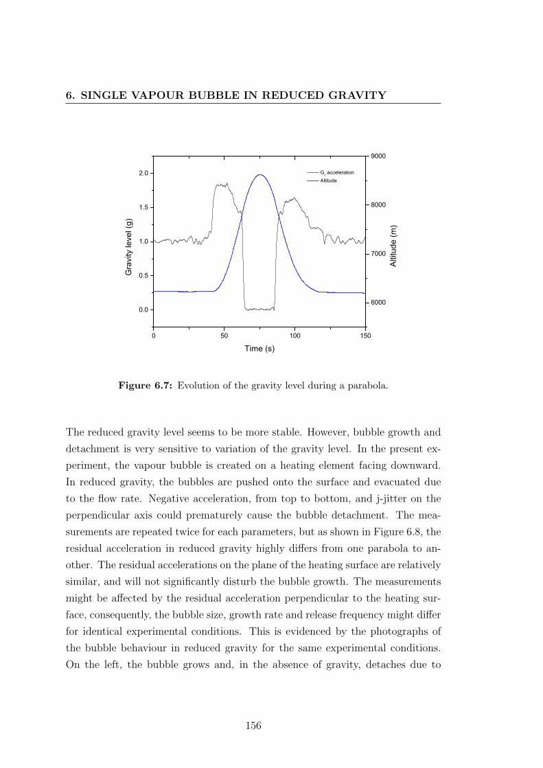
6. SINGLE VAPOUR BUBBLE IN REDUCED GRAVITY
0 50 100 150
0.0
0.5
1.0
1.5
2.0 Gz acceleration Altitude
Time (s)
Gra
vity
leve
l (g)
6000
7000
8000
9000
Alti
tude
(m)
Figure 6.7: Evolution of the gravity level during a parabola.
The reduced gravity level seems to be more stable. However, bubble growth and
detachment is very sensitive to variation of the gravity level. In the present ex-
periment, the vapour bubble is created on a heating element facing downward.
In reduced gravity, the bubbles are pushed onto the surface and evacuated due
to the flow rate. Negative acceleration, from top to bottom, and j-jitter on the
perpendicular axis could prematurely cause the bubble detachment. The mea-
surements are repeated twice for each parameters, but as shown in Figure 6.8, the
residual acceleration in reduced gravity highly differs from one parabola to an-
other. The residual accelerations on the plane of the heating surface are relatively
similar, and will not significantly disturb the bubble growth. The measurements
might be affected by the residual acceleration perpendicular to the heating sur-
face, consequently, the bubble size, growth rate and release frequency might differ
for identical experimental conditions. This is evidenced by the photographs of
the bubble behaviour in reduced gravity for the same experimental conditions.
On the left, the bubble grows and, in the absence of gravity, detaches due to
156
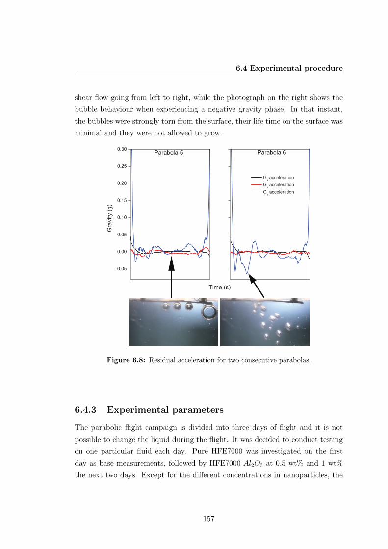
6.4 Experimental procedure
shear flow going from left to right, while the photograph on the right shows the
bubble behaviour when experiencing a negative gravity phase. In that instant,
the bubbles were strongly torn from the surface, their life time on the surface was
minimal and they were not allowed to grow.
Figure 6.8: Residual acceleration for two consecutive parabolas.
6.4.3 Experimental parameters
The parabolic flight campaign is divided into three days of flight and it is not
possible to change the liquid during the flight. It was decided to conduct testing
on one particular fluid each day. Pure HFE7000 was investigated on the first
day as base measurements, followed by HFE7000-Al2O3 at 0.5 wt% and 1 wt%
the next two days. Except for the different concentrations in nanoparticles, the
157
6. SINGLE VAPOUR BUBBLE IN REDUCED GRAVITY
other parameters to be varied during the flight included the heat flux and mass
flow rate. The choice of these parameters was triggered by the flight schedule
as the parabolas are performed in sets of five. At the end of each set, a small
break allows the experimenter to modify the experimental conditions. In the case
of this study, the flight was divided into three periods, where the flow rate was
changed, since it is difficult to modify it between two parabolas. The flow rates
investigated in reduced gravity were 0.1, 1 and 2 ml.min−1. The heat flux, being
easily set, was changed from one parabola to another. Heat fluxes were varied
between 1 and 5 W.cm−2. In order to ensure some repeatability, the measure-
ments were repeated twice over two consecutive parabolas.
Comparison of the bubble growth behaviour of pure liquid and nanofluid in vari-
able gravity will mostly rely on the acquisition of the nucleation site temperature
and the variations in the bubble detachment radius as a function of the gravity
level. However, due to the experimental conditions, uncertainties in the measure-
ment were increased.
In the same manner as in the previous chapter, the temperature is obtained
through infrared measurements. The change of the infrared camera induced
higher uncertainties in the temperature determination. An uncertainty of± 0.5C
in the nucleation site temperature was estimated.
The geometrical characteristics, including the wetting diameter, bubble maxi-
mum diameter and height, are determined by measuring directly on the visible
camera images. The uncertainties in the position of the vapour bubble interface
was estimated to be ± 4 pixels corresponding to 0.0625 mm.
The uncertainties in the heat fluxes and flow rates are the same as the one de-
scribed in the previous chapters. When multiple data points were obtained for
given experimental parameters, the standard deviation method was applied to
reduce the data to a single data point.
158
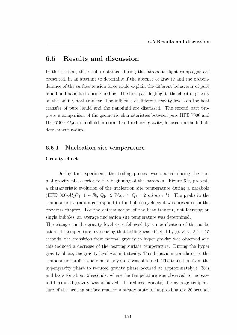
6.5 Results and discussion
6.5 Results and discussion
In this section, the results obtained during the parabolic flight campaigns are
presented, in an attempt to determine if the absence of gravity and the prepon-
derance of the surface tension force could explain the different behaviour of pure
liquid and nanofluid during boiling. The first part highlights the effect of gravity
on the boiling heat transfer. The influence of different gravity levels on the heat
transfer of pure liquid and the nanofluid are discussed. The second part pro-
poses a comparison of the geometric characteristics between pure HFE 7000 and
HFE7000-Al2O3 nanofluid in normal and reduced gravity, focused on the bubble
detachment radius.
6.5.1 Nucleation site temperature
Gravity effect
During the experiment, the boiling process was started during the nor-
mal gravity phase prior to the beginning of the parabola. Figure 6.9, presents
a characteristic evolution of the nucleation site temperature during a parabola
(HFE7000-Al2O3, 1 wt%, Qp=2 W.m−2, Qv= 2 ml.min−1). The peaks in the
temperature variation correspond to the bubble cycle as it was presented in the
previous chapter. For the determination of the heat transfer, not focusing on
single bubbles, an average nucleation site temperature was determined.
The changes in the gravity level were followed by a modification of the nucle-
ation site temperature, evidencing that boiling was affected by gravity. After 15
seconds, the transition from normal gravity to hyper gravity was observed and
this induced a decrease of the heating surface temperature. During the hyper
gravity phase, the gravity level was not steady. This behaviour translated to the
temperature profile where no steady state was obtained. The transition from the
hypergravity phase to reduced gravity phase occured at approximately t=38 s
and lasts for about 2 seconds, where the temperature was observed to increase
until reduced gravity was achieved. In reduced gravity, the average tempera-
ture of the heating surface reached a steady state for approximately 20 seconds
159

6. SINGLE VAPOUR BUBBLE IN REDUCED GRAVITY
despite the residual acceleration. At the end of the microgravity segment, the
transition to another hypergravity phase was characterized by a sudden decrease
in the nucleation site temperature. For data storage issues, the second phase of
hypergravity was usually not studied.
Figure 6.9: Nucleation site temperature evolution during a parabola (HFE7000-
Al2O3, 1 wt%, Qp=2 W.m−2, Qv= 2 ml.min−1).
It was observed that the nucleation site temperature was modified during the
different phases of the parabola. The highest temperatures were usually observed
during the reduced gravity phase, evidencing deterioration in the heat transfer.
This is confirmed by Figure 6.10, where the nucleation site temperatures are plot-
ted as a function of the imposed heat flux for a flow rate of 0.1 ml.min−1. The
temperature values are an averaged value over a period of at least ten seconds,
except for the hypergravity phase where the gravity level is not constant and
was estimated over two seconds approximately. The heat flux varied from 1 to
5 W.cm−2 , which only represents a minimum part of the boiling curve. Below
160

6.5 Results and discussion
these heat fluxes, no bubble was observed and above multiple bubbles were cre-
ated. The measurement errors on the temperature have been estimated to be
approximately 0.5K. The results presented for the temperature evolution should
be carefully considered, since the temperature variations are really small and sen-
sitive to the experimental conditions in the plane.
Increasing gravity level
Figure 6.10: Boiling curves at different gravity levels (HFE7000-Al2O3, 1 wt%,
Qv= 0.1 ml.min−1).
For a constant gravity level, an increase in the nucleation site temperature is
observed with the increase of the imposed heat flux. For a constant heat flux, an
increase in the gravity level leads to a decrease in the nucleation site temperature.
This is evidenced on the graph with a shift to the left of the curves when the
gravity level is increased. The observation can also be made that the trends of
the curves are not modified with the gravity level.
This behaviour demonstrates an enhancement in the heat transfer with an in-
crease in the gravity level. Actually, an increase in the gravity level was ac-
161
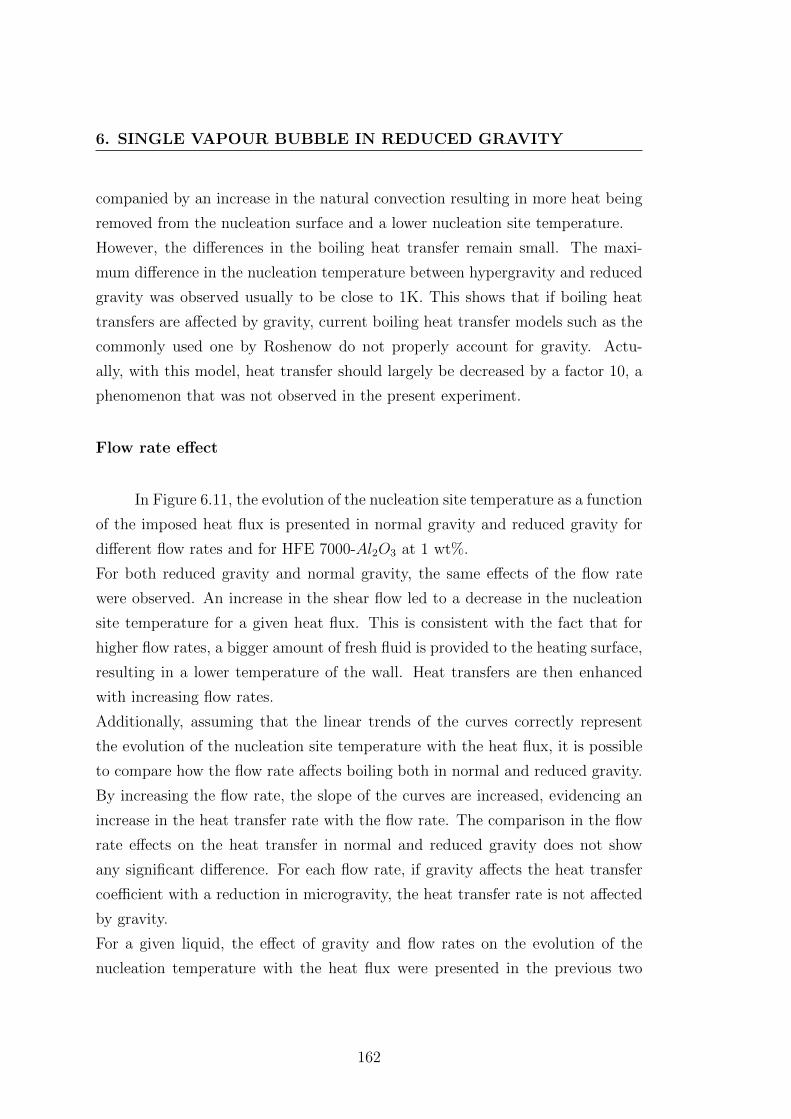
6. SINGLE VAPOUR BUBBLE IN REDUCED GRAVITY
companied by an increase in the natural convection resulting in more heat being
removed from the nucleation surface and a lower nucleation site temperature.
However, the differences in the boiling heat transfer remain small. The maxi-
mum difference in the nucleation temperature between hypergravity and reduced
gravity was observed usually to be close to 1K. This shows that if boiling heat
transfers are affected by gravity, current boiling heat transfer models such as the
commonly used one by Roshenow do not properly account for gravity. Actu-
ally, with this model, heat transfer should largely be decreased by a factor 10, a
phenomenon that was not observed in the present experiment.
Flow rate effect
In Figure 6.11, the evolution of the nucleation site temperature as a function
of the imposed heat flux is presented in normal gravity and reduced gravity for
different flow rates and for HFE 7000-Al2O3 at 1 wt%.
For both reduced gravity and normal gravity, the same effects of the flow rate
were observed. An increase in the shear flow led to a decrease in the nucleation
site temperature for a given heat flux. This is consistent with the fact that for
higher flow rates, a bigger amount of fresh fluid is provided to the heating surface,
resulting in a lower temperature of the wall. Heat transfers are then enhanced
with increasing flow rates.
Additionally, assuming that the linear trends of the curves correctly represent
the evolution of the nucleation site temperature with the heat flux, it is possible
to compare how the flow rate affects boiling both in normal and reduced gravity.
By increasing the flow rate, the slope of the curves are increased, evidencing an
increase in the heat transfer rate with the flow rate. The comparison in the flow
rate effects on the heat transfer in normal and reduced gravity does not show
any significant difference. For each flow rate, if gravity affects the heat transfer
coefficient with a reduction in microgravity, the heat transfer rate is not affected
by gravity.
For a given liquid, the effect of gravity and flow rates on the evolution of the
nucleation temperature with the heat flux were presented in the previous two
162
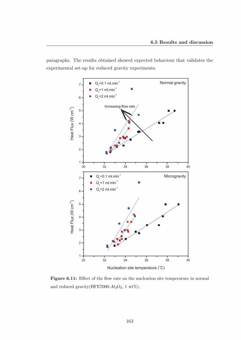
6.5 Results and discussion
paragraphs. The results obtained showed expected behaviour that validates the
experimental set-up for reduced gravity experiments.
Increasing ow rate
Figure 6.11: Effect of the flow rate on the nucleation site temperature in normal
and reduced gravity(HFE7000-Al2O3, 1 wt%).
163
6. SINGLE VAPOUR BUBBLE IN REDUCED GRAVITY
Comparison between pure HFE7000 and HFE7000-Al2O3 in reduced
gravity
It was shown, in the previous chapters, that boiling heat transfer is en-
hanced in normal gravity with the HFE7000-Al2O3 nanofluids as compared with
pure HFE7000. The nucleation site temperature was found to be lower with
nanofluid, evidencing a local increase of the heat transfer.
In Figure 6.12, the nucleation site temperature is plotted as a function of the im-
posed heat flux for pure HFE7000 and HFE7000-Al2O3 at 1 wt% for two constant
flow rates in reduced gravity. Experiments with HFE7000-Al2O3 at 0.5 wt% were
also performed, but due to some experimental failures, only very little data under
the same conditions were obtained, which did not allow a good comparison of the
nucleation site temperature variation.
In the same manner as for the normal gravity experiment, a shift of the curve for
nanofluid to the left is observed, exhibiting a smaller nucleation site temperature
and an increase in the heat transfer for HFE7000-Al2O3 at 1 wt% as compared
with pure HFE7000. For the low flow rates investigated here, Qv=1 ml.min−1
and Qv=2 ml.min−1, the slopes were found to be similar, exhibiting a smaller
nucleation site temperature to an increase in the heat flux for the nanofluid as
compared to pure HFE7000.
Despite the significant measurement errors due to the experimental conditions
in the plane, an average nucleation site temperature difference by approximately
0.5K to 0.7K is observed between pure liquid and the nanofluid. It is consistent
with the temperature variation obtained during ground experiments as shown in
the previous chapter. Unfortunately, due to experimental difficulties onboard the
plane, it was not possible to obtain reliable temperature data points for both
fluids at different gravity levels and flow rates. If reduced gravity data were usu-
ally obtained, in normal gravity and even more in hyper gravity, the experiments
were often perturbed by massive vapour bubbles stuck on the heating surface,
preventing the bubbles nucleation. The variation in the nucleation site temper-
ature in reduced gravity are in the same order as those obtained during ground
experiments, as shown in the previous chapter. The gravity level does not have
164
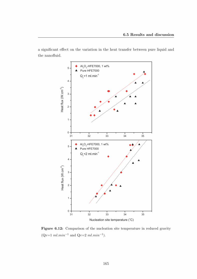
6.5 Results and discussion
a significant effect on the variation in the heat transfer between pure liquid and
the nanofluid.
Figure 6.12: Comparison of the nucleation site temperature in reduced gravity
(Qv=1 ml.min−1 and Qv=2 ml.min−1).
165
6. SINGLE VAPOUR BUBBLE IN REDUCED GRAVITY
6.5.2 Bubble size
Gravity effect
During the different phases of the parabola, the bubble shape and size were
modified. During hypergravity phases, the bubble was pushed upward on the
surface and the bubble shape was flattened onto the surface, in normal gravity,
the bubble has the shape of a spherical cap pushed onto the surface, while in
reduced gravity the bubble was fully circular in the two dimension cell.
During parabolic flight experiments, the bubble sizes were higher than those
obtained in the lab because of changes in the working pressure and liquid sat-
uration temperature. During laboratory experiments, the bubble diameter was
always lower than the size of the experimental cell confinement (1mm), while in
the present experiment, the diameter was, in most of the cases, higher than the
cell thickness. The detachment radius, in normal gravity, was then calculated
based on the measurement of the bubble height, maximum diameter and wetting
diameter, when accessible. The dimensions of the bubbles being still in the same
order as the capillary length, the bubble was assumed to have a two-dimensional
spherical cap shape, and a width equal to the confinement thickness. In reduced
gravity, the bubble is spherical and its volume was calculated as a 1mm slice of
a sphere. The curvature of the bubble was neglected. After calculation of the
bubble volume, the radius at detachment of an equivalent sphere was calculated,
to compare radius in normal gravity and reduced gravity.
The gravity influence on the bubble size at detachment is presented in Figure
6.13, where the vapour bubble radius at detachment is plotted as a function of
the imposed heat flux in normal and reduced gravity. It is observed that the
bubble radius at detachment remains roughly constant with the increase in the
imposed heat flux in normal and reduced gravity. However, the bubble radius
at detachment is found to be always smaller in reduced gravity than in normal
gravity. This sounds contradictory with results published in the literature, where
the bubble was usually observed to be much bigger in microgravity. However,
in the present experiment, the bubble is created on a downward facing heating
166
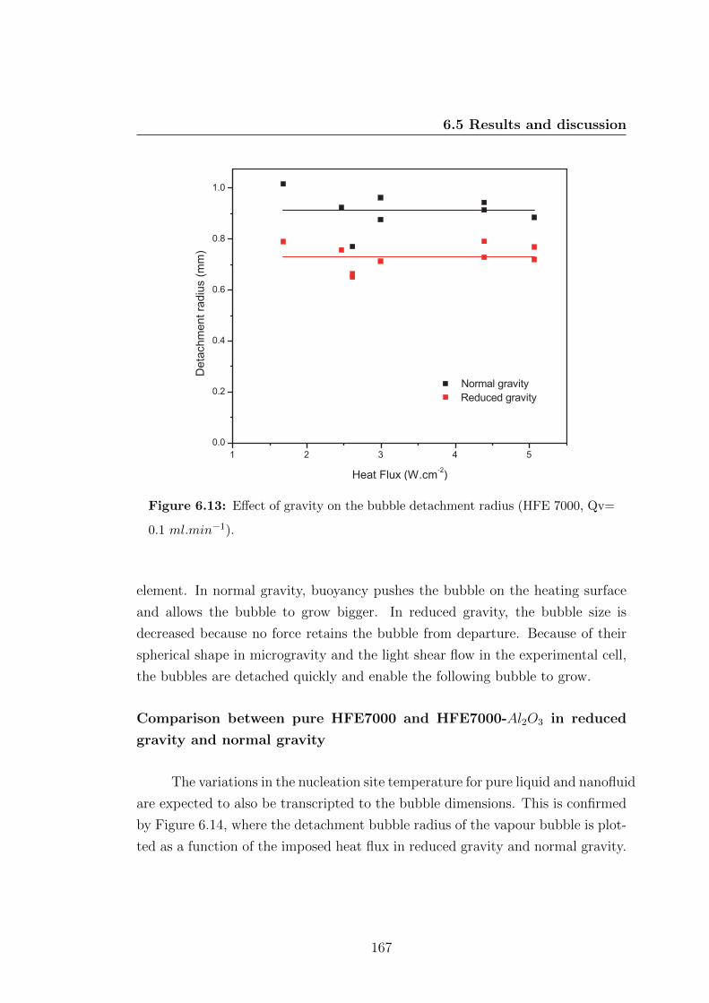
6.5 Results and discussion
Figure 6.13: Effect of gravity on the bubble detachment radius (HFE 7000, Qv=
0.1 ml.min−1).
element. In normal gravity, buoyancy pushes the bubble on the heating surface
and allows the bubble to grow bigger. In reduced gravity, the bubble size is
decreased because no force retains the bubble from departure. Because of their
spherical shape in microgravity and the light shear flow in the experimental cell,
the bubbles are detached quickly and enable the following bubble to grow.
Comparison between pure HFE7000 and HFE7000-Al2O3 in reduced
gravity and normal gravity
The variations in the nucleation site temperature for pure liquid and nanofluid
are expected to also be transcripted to the bubble dimensions. This is confirmed
by Figure 6.14, where the detachment bubble radius of the vapour bubble is plot-
ted as a function of the imposed heat flux in reduced gravity and normal gravity.
167
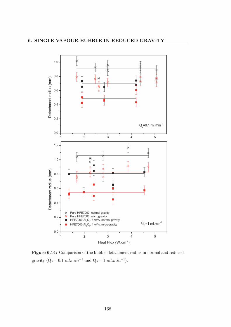
6. SINGLE VAPOUR BUBBLE IN REDUCED GRAVITY
Figure 6.14: Comparison of the bubble detachment radius in normal and reduced
gravity (Qv= 0.1 ml.min−1 and Qv= 1 ml.min−1).
168
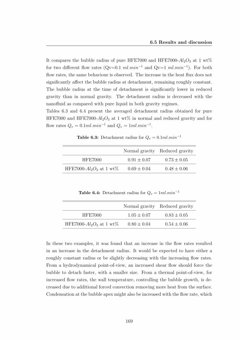
6.5 Results and discussion
It compares the bubble radius of pure HFE7000 and HFE7000-Al2O3 at 1 wt%
for two different flow rates (Qv=0.1 ml.min−1 and Qv=1 ml.min−1). For both
flow rates, the same behaviour is observed. The increase in the heat flux does not
significantly affect the bubble radius at detachment, remaining roughly constant.
The bubble radius at the time of detachment is significantly lower in reduced
gravity than in normal gravity. The detachment radius is decreased with the
nanofluid as compared with pure liquid in both gravity regimes.
Tables 6.3 and 6.4 present the averaged detachment radius obtained for pure
HFE7000 and HFE7000-Al2O3 at 1 wt% in normal and reduced gravity and for
flow rates Qv = 0.1ml.min−1 and Qv = 1ml.min−1.
Table 6.3: Detachment radius for Qv = 0.1ml.min−1
Normal gravity Reduced gravity
HFE7000 0.91± 0.07 0.73± 0.05
HFE7000-Al2O3 at 1 wt% 0.69± 0.04 0.48± 0.06
Table 6.4: Detachment radius for Qv = 1ml.min−1
Normal gravity Reduced gravity
HFE7000 1.05± 0.07 0.83± 0.05
HFE7000-Al2O3 at 1 wt% 0.80± 0.04 0.54± 0.06
In these two examples, it was found that an increase in the flow rates resulted
in an increase in the detachment radius. It would be expected to have either a
roughly constant radius or be slightly decreasing with the increasing flow rates.
From a hydrodynamical point-of-view, an increased shear flow should force the
bubble to detach faster, with a smaller size. From a thermal point-of-view, for
increased flow rates, the wall temperature, controlling the bubble growth, is de-
creased due to additional forced convection removing more heat from the surface.
Condensation at the bubble apex might also be increased with the flow rate, which
169
6. SINGLE VAPOUR BUBBLE IN REDUCED GRAVITY
should then logically affect the bubble radius at the time of detachment. How-
ever, taking into account the measurement uncertainties on the bubble dimension,
the sensitive experimental conditions and the low flow rates investigated, it will
be assumed that low flow rate has a minimal impact on the bubble detachment
radius.
In order to verify the consistency of the results obtained, a comparison of the
experimental data and models predicting the bubble diameter at detachment is
presented in Figure 6.15. It compares the experimental evolution of the detach-
ment radius of pure HFE7000 and HFE7000-Al2O3 at 1 wt% with the models
presented in the literature review. The experimental data of heat fluxes and
nucleation site temperature for pure HFE7000 are used in the models and the
gravity level in reduced gravity is assumed to be gµg = 5.10−2g.
These models were proposed, based on the balance of the forces acting on the
bubble, in normal gravity. In these models, the detachment diameter is grav-
ity dependent and evolved as Dd ≈ g−1/2 or Dd ≈ g−1/3. Experimental studies
published in the literature showed good agreement with these predictions. In
the case of this study, the models are not valid in normal gravity because of
the special configuration of the heating element facing downward. However, in
a reduced gravity environment, the experimental data becomes comparable due
to the gravity-driven buoyancy force being removed. All the models presented in
the literature review were compared, except for the model proposed by Fritz (42).
This model relies on the contact angle between the bubble and the surface at de-
tachment. This could not be determined due to the data acquisition restrictions
that only allowed the visualisation of the bubble right after it was detached from
the nucleation site and there was no observation of the contact angle. Since all the
models are based on the experimental data of the nucleation site temperature and
heat flux, the same dispersion in the data point is observed for the models. De-
spite the fact that all these models are based on a force balance made for a bubble
facing upward, the data obtained in reduced gravity in this research are relatively
consistent with published models. These models underestimate the detachment
radius as compared to the data obtained in this research. The closest models are
nevertheless those accounting mostly for the thermophysical properties and wall
170
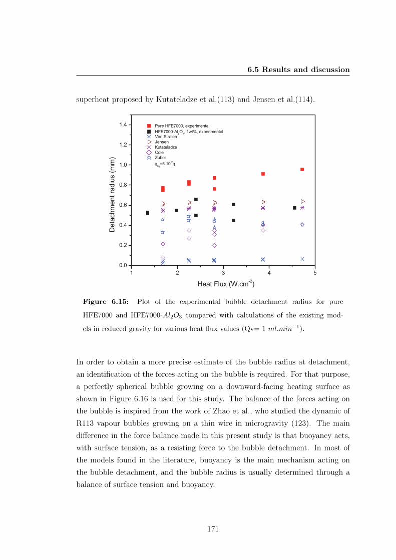
6.5 Results and discussion
superheat proposed by Kutateladze et al.(113) and Jensen et al.(114).
Figure 6.15: Plot of the experimental bubble detachment radius for pure
HFE7000 and HFE7000-Al2O3 compared with calculations of the existing mod-
els in reduced gravity for various heat flux values (Qv= 1 ml.min−1).
In order to obtain a more precise estimate of the bubble radius at detachment,
an identification of the forces acting on the bubble is required. For that purpose,
a perfectly spherical bubble growing on a downward-facing heating surface as
shown in Figure 6.16 is used for this study. The balance of the forces acting on
the bubble is inspired from the work of Zhao et al., who studied the dynamic of
R113 vapour bubbles growing on a thin wire in microgravity (123). The main
difference in the force balance made in this present study is that buoyancy acts,
with surface tension, as a resisting force to the bubble detachment. In most of
the models found in the literature, buoyancy is the main mechanism acting on
the bubble detachment, and the bubble radius is usually determined through a
balance of surface tension and buoyancy.
171
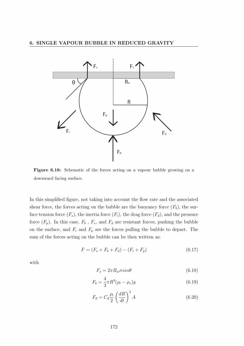
6. SINGLE VAPOUR BUBBLE IN REDUCED GRAVITY
θ
Fb
Fs Fs
Fp
Fi Fd
Rw
R
Figure 6.16: Schematic of the forces acting on a vapour bubble growing on a
downward facing surface.
In this simplified figure, not taking into account the flow rate and the associated
shear force, the forces acting on the bubble are the buoyancy force (Fb), the sur-
face tension force (Fs), the inertia force (Fi), the drag force (Fd), and the pressure
force (Fp). In this case, Fb , Fs, and Fd are resistant forces, pushing the bubble
on the surface, and Fi and Fp are the forces pulling the bubble to depart. The
sum of the forces acting on the bubble can be then written as:
F = (Fs + Fb + Fd)− (Fi + Fp) (6.17)
with
Fs = 2πRwσsinθ (6.18)
Fb =4
3πR3(ρl − ρv)g (6.19)
Fd = Cdρl2
(dR
dt
)2
A (6.20)
172
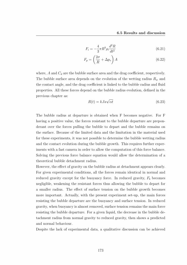
6.5 Results and discussion
Fi = −4
3πR3ρl
d2R
dt2(6.21)
Fp =
(2σ
R+ ∆pv
)A (6.22)
where, A and Cd are the bubble surface area and the drag coefficient, respectively.
The bubble surface area depends on the evolution of the wetting radius Rw and
the contact angle, and the drag coefficient is linked to the bubble radius and fluid
properties. All these forces depend on the bubble radius evolution, defined in the
previous chapter as:
R(t) = kJa√αt (6.23)
The bubble radius at departure is obtained when F becomes negative. For F
having a positive value, the forces resistant to the bubble departure are prepon-
derant over the forces pulling the bubble to depart and the bubble remains on
the surface. Because of the limited data and the limitation in the material used
for these experiments, it was not possible to determine the bubble wetting radius
and the contact evolution during the bubble growth. This requires further exper-
iments with a fast camera in order to allow the computation of this force balance.
Solving the previous force balance equation would allow the determination of a
theoretical bubble detachment radius.
However, the effect of gravity on the bubble radius at detachment appears clearly.
For given experimental conditions, all the forces remain identical in normal and
reduced gravity except for the buoyancy force. In reduced gravity, Fb becomes
negligible, weakening the resistant forces thus allowing the bubble to depart for
a smaller radius. The effect of surface tension on the bubble growth becomes
more important. Actually, with the present experiment set-up, the main forces
resisting the bubble departure are the buoyancy and surface tension. In reduced
gravity, when buoyancy is almost removed, surface tension remains the main force
resisting the bubble departure. For a given liquid, the decrease in the bubble de-
tachment radius from normal gravity to reduced gravity, then shows a predicted
and normal behaviour.
Despite the lack of experimental data, a qualitative discussion can be achieved
173
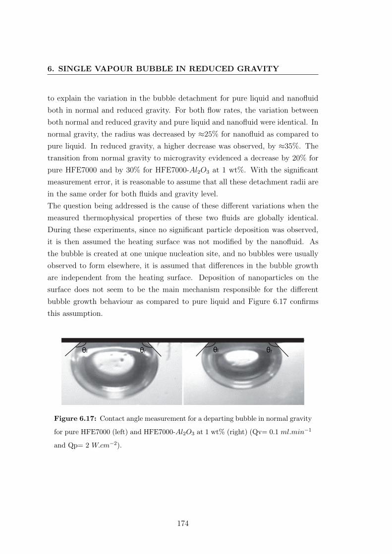
6. SINGLE VAPOUR BUBBLE IN REDUCED GRAVITY
to explain the variation in the bubble detachment for pure liquid and nanofluid
both in normal and reduced gravity. For both flow rates, the variation between
both normal and reduced gravity and pure liquid and nanofluid were identical. In
normal gravity, the radius was decreased by ≈25% for nanofluid as compared to
pure liquid. In reduced gravity, a higher decrease was observed, by ≈35%. The
transition from normal gravity to microgravity evidenced a decrease by 20% for
pure HFE7000 and by 30% for HFE7000-Al2O3 at 1 wt%. With the significant
measurement error, it is reasonable to assume that all these detachment radii are
in the same order for both fluids and gravity level.
The question being addressed is the cause of these different variations when the
measured thermophysical properties of these two fluids are globally identical.
During these experiments, since no significant particle deposition was observed,
it is then assumed the heating surface was not modified by the nanofluid. As
the bubble is created at one unique nucleation site, and no bubbles were usually
observed to form elsewhere, it is assumed that differences in the bubble growth
are independent from the heating surface. Deposition of nanoparticles on the
surface does not seem to be the main mechanism responsible for the different
bubble growth behaviour as compared to pure liquid and Figure 6.17 confirms
this assumption.
θl θl θr θr
Figure 6.17: Contact angle measurement for a departing bubble in normal gravity
for pure HFE7000 (left) and HFE7000-Al2O3 at 1 wt% (right) (Qv= 0.1 ml.min−1
and Qp= 2 W.cm−2).
174
6.5 Results and discussion
This figure compares the contact angle of a vapour bubble created in normal
gravity for pure liquid (left) and the nanofluid (right) just prior to departure
from the nucleation site. For the left contact angle, θl, contact angles of 132
and 131 were obtained for pure liquid and nanofluid, respectively. The measure-
ment of the right contact angle, θr, corresponding to the side of the bubble not
facing the flow, was 143 and 139, for pure HFE7000 and the nanofluid, respec-
tively. The detachment of the vapour bubble occurs for similar contact angles
with pure liquid and the nanofluid; modification of the wettability is not the main
mechanism responsible for the bubble growth. Evaluation of the contact angle in
reduced gravity was not possible with the current experimental set-up, the bubble
growth rate being too high to be recorded; the bubbles were only observable just
after their detachment. Since the surface was not modified, the contact angle
in reduced gravity is expected to be similar for pure liquid and the nanofluid
in the same manner as in normal gravity. The differences in the bubble radius
at detachment between pure liquid and the nanofluid for a given gravity level,
support the concept that wettability cannot fully explain these differences. The
variations in normal gravity are similar to those in reduced gravity. If wettabilty
and surface tension were the main parameters governing the bubble detachment,
in reduced gravity, when surface tension force is preponderant over buoyancy, it
would have been expected to obtain significant changes in the detachment radius
of nanofluid.
However, the nucleation site will need to be investigated through SEM mea-
surement to validate this hypothesis. Because of the actual configuration of the
experimental cell, this could not be achieved without permanently damaging the
cell and the heating surface.
If the modification of the surface cannot fully explain the variation in the bubble
radius at detachment between pure liquid and the nanofluid, and accounting for
similar global properties of the fluids, it implies a local modification of the bubble
growth mechanisms. It was shown in the previous chapter, that bubble growth is
mainly governed by the evaporation of the microlayer, where the concentration
in nanoparticles can be drastically enhanced. For the reduced gravity data pre-
sented here, the same phenomenon can explain the bubble radius variation. For a
175
6. SINGLE VAPOUR BUBBLE IN REDUCED GRAVITY
given liquid, the transition from normal to reduced gravity evidence variation in
the same order of magnitude both for pure HFE7000 and for HFE7000-Al2O3 at
1 wt%, and the same order of variation is obtained when comparing the detach-
ment radius of each fluid for one given gravity level. Removing the buoyancy force
has the same effect for both liquids, giving more weight to surface tension force
as a mechanism counteracting the bubble detachment, showing surface tension
does not seem to be more preponderant for the nanofluid than for pure liquid.
In the same manner as for normal gravity experiments, the main explanation for
bubble growth difference in reduced gravity is given by the local modification of
the liquid properties during the microlayer evaporation.
6.6 Conclusions
In this chapter, preliminary results on the bubble growth of nanofluid were pre-
sented. Effects of gravity on the nucleation site temperature and bubble de-
tachment radius were discussed. It was expected that in reduced gravity, effects
masked by gravity such as surface tension would be revealed.
The temperature measurements show expected results, where the nucleation site
temperature is decreased with a increase of the gravity level. This can be ex-
plained by the convective heat transfer enhancement. Differences in the tem-
perature for pure liquid and the nanofluid in reduced gravity follow the same
behaviour as for ground experiments. Both for normal gravity and reduced grav-
ity, the heat transfer properties are slightly increased with HFE7000-Al2O3 at 1
wt% as compared with pure HFE7000.
The determination of the bubble growth rate in reduced gravity was unfortunately
not possible with the current experimental set-up. However it was possible to de-
termine the variation in the bubble detachment diameter both in normal and
reduced gravity for pure liquid and the nanofluid. The behaviour due to the dif-
ferent gravity levels was expected, with a decrease in the detachment radius in
reduced gravity as compared with normal gravity. When comparing the variation
in the radius between pure liquid and the nanofluid in microgravity, the same or-
der of variation was observed as in a normal gravity environment. This showed
176
6.6 Conclusions
that surface tension is not the main mechanism responsible for the changes in the
growth behaviour of nanofluid. Variations in the bubble growth seem to be due
to a local modification of the thermophysical properties in the microlayer due to
an increase in the nanoparticle concentration in this area during its evaporation.
Objectives for future work will be to perform more experiments on a wider range
of heat flux, to cover the full boiling curve until the critical heat flux is achieved,
to redesign the fluid loop to prevent loss of data in normal and hyper gravity,
change the data acquisition system in order to be able to follow the bubble growth
from its nucleation until its detachment, focusing on the wetting diameter, and
the evolution of the contact angle and a link with the bubble release frequency.
Other nanofluids and concentrations will need to be studied as well. A theoret-
ical approach on the bubble growth and detachment is also required. Solving
the balance of the force acting on the bubble during its growth will allow the
determination of the detachment radius for this particular configuration where
the bubble is created on a downward facing heating surface.
177
6. SINGLE VAPOUR BUBBLE IN REDUCED GRAVITY
178
7
Qualitative bubble growth model
The measurements and observations made in Chapters 5 and 6, at the scale of
single vapour bubbles in pure HFE7000 and HFE7000-Al2O30 nanofluid, in nor-
mal and reduced gravity, evidenced a bubble growth behaviour summarized in
this section. The bubbles are created on a single artificial nucleation site on a
downward-facing heating surface where a constant heat flux is applied.
When comparing nucleate boiling of pure HFE7000 and the HFE7000-Al2O3
nanofluid at 1wt% for a constant heat flux, the following geometrical observa-
tions were made (or postulated in reduced gravity):
1. The bubble radius at detachment is lower for nanofluid.
2. The bubble release frequency is higher for nanofluid. Bubble growth time
was found similar while the waiting period is shortened with nanofluid.
3. The contact angle is similar for both fluids.
4. The bubble radius at detachment is lower in reduced gravity.
5. The bubble release frequency is higher in reduced gravity.
6. The bubble radius time evolution is written as R(t) = kJa√αt.
179
7. QUALITATIVE BUBBLE GROWTH MODEL
The thermophysical properties of pure HFE7000 and HFE7000-Al2O3 nanofluid
at 1wt% measured were similar and there is no significant difference. The bubble
growth cycle comparing pure liquid and nanofluid is as follows:
t1: In the first stage of the growth, just after nucleation, the bubble is governed
by inertial effect produced by the movement of the liquid- vapour interface.
The shape of the bubble is hemispherical and a liquid microlayer appears
under the bubble. The bubble size is identical for pure liquid and nanofluid.
t2-t3: During the bubble growth, the vapour bubble tends to have a spherical
like shape. The bubble growth is governed by the evaporating microlayer,
leading to the expansion of a dry area under the vapour bubble. Differences
in the bubble size between pure liquid and the nanofluid increase with the
increasing bubble growth time.
td: Finally, when the surface tension and buoyancy forces become lower than
the other forces (shear, inertia, pressure), the bubble is departing from the
nucleation site. After the waiting period, the cycle restarts. The radius at
detachment is significantly lower for the nanofluid than for pure liquid. The
bubble growth time is similar for both fluids, however waiting period being
lower for the nanofluid, a new bubble growth cycle will occur faster.
Figure 7.1 presents a schematic comparison of the bubble growth of pure liquid
and the nanofluid from nucleation to detachment in normal and reduced gravity.
During ground experiments, it was possible to follow the geometrical evolution
of the bubbles. In reduced gravity, the bubble radius at departure could only be
measured.
If in normal gravity, the sphere-like shape of the vapour bubble can be flattened
by the buoyant force, depending on the bubble size, in reduced gravity the shape
of the bubble remains perfectly spherical. In reduced gravity, the bubble nucle-
ation, growth and detachment cycle is shorter than in normal gravity. When
buoyancy force is not acting on the bubble, surface tension becomes the main
mechanism restraining the bubble to depart from the nucleation site. As a re-
sult, the bubble radius at detachment is decreased as compared to that in normal
gravity. In reduced gravity, the variations in the detachment radius between pure
180
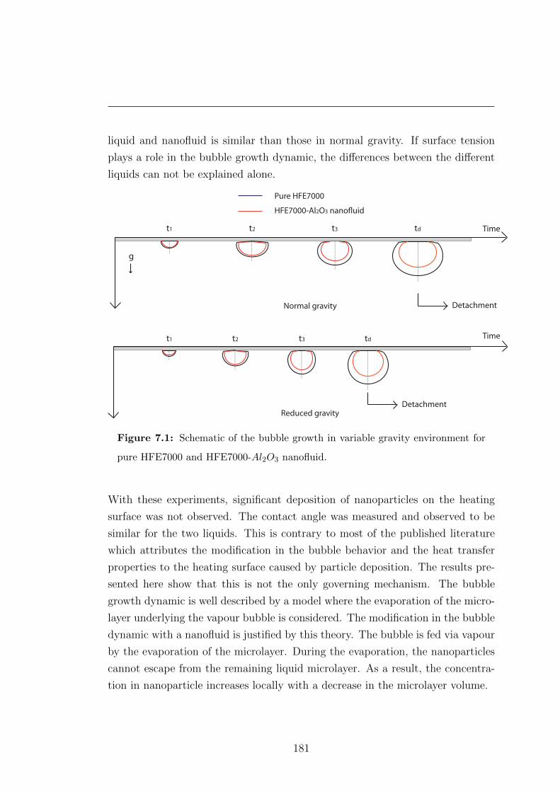
liquid and nanofluid is similar than those in normal gravity. If surface tension
plays a role in the bubble growth dynamic, the differences between the different
liquids can not be explained alone.
Pure HFE7000
HFE7000-Al2O3 nanouid
Detachment
Detachment
Normal gravity
Reduced gravity
Time
Timet1 t2 t3 td
t1 t2 t3 td
g
Figure 7.1: Schematic of the bubble growth in variable gravity environment for
pure HFE7000 and HFE7000-Al2O3 nanofluid.
With these experiments, significant deposition of nanoparticles on the heating
surface was not observed. The contact angle was measured and observed to be
similar for the two liquids. This is contrary to most of the published literature
which attributes the modification in the bubble behavior and the heat transfer
properties to the heating surface caused by particle deposition. The results pre-
sented here show that this is not the only governing mechanism. The bubble
growth dynamic is well described by a model where the evaporation of the micro-
layer underlying the vapour bubble is considered. The modification in the bubble
dynamic with a nanofluid is justified by this theory. The bubble is fed via vapour
by the evaporation of the microlayer. During the evaporation, the nanoparticles
cannot escape from the remaining liquid microlayer. As a result, the concentra-
tion in nanoparticle increases locally with a decrease in the microlayer volume.
181
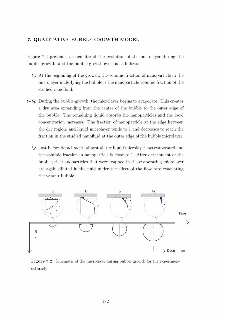
7. QUALITATIVE BUBBLE GROWTH MODEL
Figure 7.2 presents a schematic of the evolution of the microlayer during the
bubble growth, and the bubble growth cycle is as follows:
t1: At the beginning of the growth, the volumic fraction of nanoparticle in the
microlayer underlying the bubble is the nanoparticle volumic fraction of the
studied nanofluid.
t2-t3: During the bubble growth, the microlayer begins to evaporate. This creates
a dry area expanding from the center of the bubble to the outer edge of
the bubble. The remaining liquid absorbs the nanoparticles and the local
concentration increases. The fraction of nanoparticle at the edge between
the dry region, and liquid microlayer tends to 1 and decreases to reach the
fraction in the studied nanofluid at the outer edge of the bubble microlayer.
td: Just before detachment, almost all the liquid microlayer has evaporated and
the volumic fraction in nanoparticle is close to 1. After detachment of the
bubble, the nanoparticles that were trapped in the evaporating microlayer
are again diluted in the fluid under the effect of the flow rate evacuating
the vapour bubble.
Detachment
Time
t1 t2 t3 td
g
Figure 7.2: Schematic of the microlayer during bubble growth for the experimen-
tal study.
182
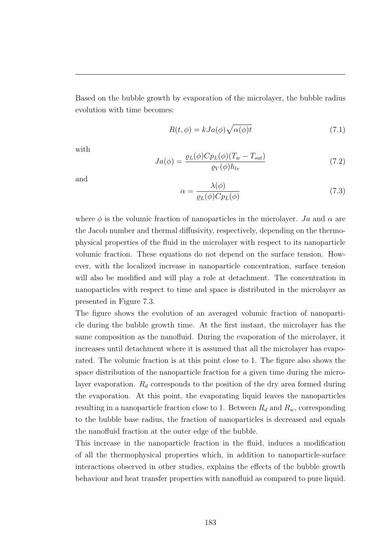
Based on the bubble growth by evaporation of the microlayer, the bubble radius
evolution with time becomes:
R(t, φ) = kJa(φ)√α(φ)t (7.1)
with
Ja(φ) =%L(φ)CpL(φ)(Tw − Tsat)
%V (φ)hlv(7.2)
and
α =λ(φ)
%L(φ)CpL(φ)(7.3)
where φ is the volumic fraction of nanoparticles in the microlayer. Ja and α are
the Jacob number and thermal diffusivity, respectively, depending on the thermo-
physical properties of the fluid in the microlayer with respect to its nanoparticle
volumic fraction. These equations do not depend on the surface tension. How-
ever, with the localized increase in nanoparticle concentration, surface tension
will also be modified and will play a role at detachment. The concentration in
nanoparticles with respect to time and space is distributed in the microlayer as
presented in Figure 7.3.
The figure shows the evolution of an averaged volumic fraction of nanoparti-
cle during the bubble growth time. At the first instant, the microlayer has the
same composition as the nanofluid. During the evaporation of the microlayer, it
increases until detachment where it is assumed that all the microlayer has evapo-
rated. The volumic fraction is at this point close to 1. The figure also shows the
space distribution of the nanoparticle fraction for a given time during the micro-
layer evaporation. Rd corresponds to the position of the dry area formed during
the evaporation. At this point, the evaporating liquid leaves the nanoparticles
resulting in a nanoparticle fraction close to 1. Between Rd and Rw, corresponding
to the bubble base radius, the fraction of nanoparticles is decreased and equals
the nanofluid fraction at the outer edge of the bubble.
This increase in the nanoparticle fraction in the fluid, induces a modification
of all the thermophysical properties which, in addition to nanoparticle-surface
interactions observed in other studies, explains the effects of the bubble growth
behaviour and heat transfer properties with nanofluid as compared to pure liquid.
183
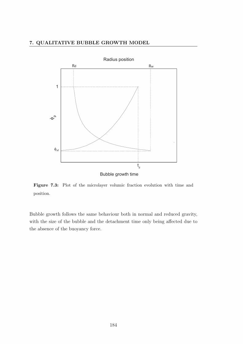
7. QUALITATIVE BUBBLE GROWTH MODEL
Rd Rw
Figure 7.3: Plot of the microlayer volumic fraction evolution with time and
position.
Bubble growth follows the same behaviour both in normal and reduced gravity,
with the size of the bubble and the detachment time only being affected due to
the absence of the buoyancy force.
184
8
Conclusions and
Recommendations
8.1 Conclusions
Nucleate boiling of pure liquid and nanofluid was experimentally investigated
under normal and reduced gravity conditions. Conclusions from this work are
presented following their order of appearance in this thesis.
1. Nanofluid preparation and characterisation
Novel nanofluids made of HFE7000 manufactured by 3M and aluminum
oxide nanoparticles (Al2O3) were prepared using the two-step method. Var-
ious concentration ranging from 0.1 to 1 wt%, were obtained and found to
be stable for over three months. Their thermophysical properties, including
density, viscosity, emissivity, surface tension and thermal conductivity were
measured and showed that they do not differ significantly with respect to
pure HFE7000. A novel method to determine the thermal conductivity was
developed based on the measurement of the thermal diffusivity taking into
account the semi transparency property of the fluid in the infrared wave-
length.
185

8. CONCLUSIONS AND RECOMMENDATIONS
2. Pool boiling of nanofluid, heat transfer coefficient and critical heat
flux
Pool boiling experiments on a thin platinum wire were performed with
the HFE7000-Al2O3 nanofluids for various subcooling and heat flux condi-
tions. Heat Transfer Coefficient (HTC) and Critical Heat Flux (CHF) were
obtained for various nanofluid concentrations. In regards to the HTC, en-
hancements of up to 23% were found for HFE7000-Al2O3 (1wt%), depend-
ing on the subcooling and heat flux. The nanofluids exhibit a significant
enhancement of up to 67% in the critical heat flux as compared to pure
HFE7000 for concentrations varying from 0.1 to 1 wt%. The CHF enhance-
ment is dependant on the nanoparticle concentration for HFE7000-Al2O3
nanofluid, increasing with the increase in the nanoparticle concentration.
Well-known correlations shown to be valid for pure liquid do not properly
account for the effects of the nanoparticles. The common explanation based
on a surface modification due to nanoparticles deposition is not fully valid
with these particular nanofluids and justifies the rest of the study.
3. Single vapour bubble dynamic of pure liquid and nanofluid
In an attempt to understand the differences in the boiling phenomena be-
tween pure liquid and nanofluids, the bubble growth dynamic of a single
vapour bubble was studied. The bubble cycle, from its nucleation to its
detachment, was observed in a Hele-Shaw cell type through infrared and
visible imaging. In the case of pure liquid, the study of a single bubble at
the interface microscale leads to a recommendation for future modelling of
bubble growth. Actually, most of the models assume an isothermal vapour
bubble temperature in which the vapour remains at the saturation cor-
responding to the pressure inside the bubble. It was shown in this study,
that despite a perfectly symmetric bubble geometry, an asymmetric thermal
186
8.1 Conclusions
growth of the liquid-vapour interface is obtained as soon as the convective
forces are dominating over the viscous forces. The assumption of constant
interface temperature is untrue and should be updated, taking into account
the local heat transfer removal effect.
The results obtained with this experimental set-up confirmed the improve-
ment in the heat transfer with nanofluids. As compared with pure liq-
uid, boiling with HFE7000-Al2O3 exhibits lower nucleation site tempera-
ture, higher bubble release frequency (≈ 30%) and smaller bubble volume
(≈ 25%). It was shown that the bubble dynamic is well-described by exist-
ing models for pure liquid, particularly those based on the evaporation of
the microlayer as the main mechanism governing the bubble growth. For
nanofluids, this mechanism implies a drastic increase in the nanoparticle
concentration in this thin layer of fluid trapped under the bubble. The
modified thermophysical properties of the fluid in this area could explain
the variation in the bubble growth dynamic and the associated heat trans-
fers.
4. Single vapour bubble in reduced gravity
The same experiments were performed in reduced gravity during parabolic
flight campaigns. The objectives were to determine if mechanisms hidden
by the buoyancy force could propose another explanation for the bubble
dynamic and heat transfer variations between pure liquid and nanofluid.
Results from this study showed that in the absence of natural convection in
reduced gravity, heat transfers are reduced with respect to a normal gravity
environment. However, the observation of the nucleation site temperature
evolution with the heat flux showed that heat transfers with nanofluid are
slightly enhanced, as compared with pure liquid for any gravity level. The
investigation in the bubble detachment radius supported this observation.
For a given gravity level, the bubble radius at detachment is always smaller
by ≈ 25% for the nanofluid than for pure liquid. These radius variations
187

8. CONCLUSIONS AND RECOMMENDATIONS
are in the same order both in normal gravity and reduced gravity, while the
forces acting on the bubble are modified, supporting the observations made
in the previous chapter, where the bubble dynamic is mostly governed by
the evaporation of the microlayer.
8.2 Future work
This research has identified the need for ongoing studies in the following direc-
tions:
1. Experimental work
Observation and characterization of the bubble growth dynamic was mostly
limited by the experimental data acquisition system. Further upgrade to
the single vapour bubble test facility should include:
a A new design in the experimental cell allowing the recovery of the
heating element for surface characterisation through SEM and EDX
analysis.
b High speed infrared and visible recording to observe the evolution of
the contact angle and wetting radius, from the bubble nucleation to
its detachment
c A modified heating surface for the observation of the evaporating mi-
crolayer during the bubble growth
One major experimental objective for future work will be to characterize
the local concentration in nanoparticles in the microlayer and determine
the evolution of the local fluid properties during the bubble growth. A
time and spatial distribution of the concentration in nanoparticles should
coupled with the visualisation of the temperature evolution in the liquid
microlayer.
188
8.2 Future work
Additional experimental parameters should also be investigated, including
different nanoparticle materials, size and concentration. Single vapour bub-
ble experiments need to be performed over a wider range of heat fluxes and
flow rates to cover both nucleate pool and flow boiling. The flow rates in-
vestigated in this study were too low to be considered as flow boiling.
2. Theoretical-Numerical work
Parallel to the experimental determination of the microlayer evolution, a
numerical investigation of the bubble growth and the effect of the nanopar-
ticles would be of great interest in completing the experimental observa-
tion. The modelling of the microlayer evaporation taking into account the
variation in the nanoparticle concentration in this area and its interaction
with the heating surface would help in predicting the bubble growth rate
and evaluating the heat transfer variation due to the nanoparticle. Such
a model would need to be completed with a modelling of the effect of the
nanoparticle along the liquid vapour interface, especially at the apex of the
bubble where recondensation might occur, and at the triple line where most
of the heat transfer occurs.
Solving the balance of the forces acting on the bubble, taking into account
the modified local properties of the fluid, is a work of the near future. It will
allow the prediction of the bubble detachment radius and bubble release
frequency both for normal and reduced gravity. Current models are not
suitable for the present experimental configuration, where vapour bubbles
are created on a downward-facing element. In this configuration, buoyancy
and surface tension forces act in the same way while they are opposed in
traditional configuration. This could be resolved when the evolution of the
contact angle and wetting radius are obtained, and can be extended both
for pool and flow boiling in normal gravity and reduced gravity.
189

8. CONCLUSIONS AND RECOMMENDATIONS
190

References
[1] Y.A. Cencel. Heat and mass transfer: a practical approach. McGraw Hill
Companies third edition, 2007. xii, 46, 48
[2] S. K. Das, N. Putra, and W. Roetzel. Pool boiling characteristics of nano-
fluids. International Journal of Heat and Mass Transfer, 46(5):851 – 862, 2003. xii, 58,
59, 63
[3] S. Soltani, S. Etemad, and J. Thibault. Pool boiling heat transfer performance
of Newtonian nanofluids. Heat and Mass Transfer, 45:1555–1560, 2009. xii, 60, 63
[4] V. P. Carey. Liquid-vapor phase-change phenomena: an introduction to the thermo-
physics of vaporization and condensation processes in heat transfer equipment. Taylor
and Francis, New York, 2008. xii, 84, 141, 143
[5] N. Ginet. Analyse des mecanismes controlant la croissance et l′ascension d′une bulle
isolee en ebullition nucleee (Analysis of the mechanisms controlling the growth and rise
of an isolated bubble during nucleate boiling). PhD thesis, INSA Cethil Lyon, 1999. xii,
90
[6] M. Steinbichler, S. Micko, and J. Straub. Nucleate boiling heat transfer on
a small hemispherical heater and a wire under microgravity. 11th International
Heat Transfer Conference, 2:539–544, 1998. xiv, 139
[7] S. U. Choi and J. A. Eastman. Enhancing thermal conductivity of fluids with
nanoparticles. Technical report, Argonne National Lab., IL (United States), 1995. 11
191
REFERENCES
[8] Y. Li, J. E. Zhou, S. Tung, E. Schneider, and S. Xi. A review on development
of nanofluid preparation and characterization. Powder Technology, 196(2):89–101,
December 2009. 12, 16, 21
[9] P. Ghosh, G. Han, M. De, C. K. Kim, and V. M. Rotello. Gold nanoparticles
in delivery applications. Advanced Drug Delivery Reviews, 60(11):1307–1315, 2008.
13
[10] M. J. Kao, C. H. Lo, T. T. Tsung, Y. Y. Wu, C. S. Jwo, and H. M. Lin.
Copper-oxide brake nanofluid manufactured using arc-submerged nanoparti-
cle synthesis system. Journal of Alloys and Compounds, 31:672–674, 2007. 13
[11] K. V. Wong and O. De Leon. Applications of nanofluids: current and future.
Advances in Mechanical Engineering, 2010, 2010. 14
[12] H. Akoh, Y. Tsukasaki, S. Yatsuya, and A. Tasaki. Magnetic properties of
ferromagnetic ultrafine particles prepared by vacuum evaporation on running
oil substrate. Journal of Crystal Growth, 45(0):495 – 500, 1978. 15
[13] J. A. Eastman, U. S. Choi, S. Li, L. J. Thompson, and S. Lee. Enhanced ther-
mal conductivity through the development of nanofluids. In Materials Research
Society Symposium Proceedings, 457, page 312, 1997. 15, 16
[14] C. H. Lo, T. T. Tsung, L. C. Chen, C. H. Su, and H. M. Lin. Fabrication
of copper oxide nanofluid using submerged arc nanoparticle synthesis system
(SANSS). Journal of Nanoparticle Research, 7(2-3):313–320, 2005. 15
[15] C. H. Lo, T. T. Tsung, and L. C. Chen. Shape-controlled synthesis of Cu-
based nanofluid using submerged arc nanoparticle synthesis system (SANSS).
Journal of Crystal Growth, 277(1-4):636–642, April 2005. 15
[16] H. T. Zhu, Y. S. Lin, and Y. S. Yin. A novel one-step chemical method
for preparation of copper nanofluids. Journal of Colloid and Interface Science,
277(1):100–103, September 2004. 15
[17] H. T. Zhu, C. Y. Zhang, Y. M. Tang, and J. X. Wang. Novel Synthesis
and Thermal Conductivity of CuO Nanofluid. Journal of Physical Chemistry C,
111(4):1646–1650, February 2007. 15
192
REFERENCES
[18] H. Zhu, C. Zhang, S. Liu, Y. Tang, and Y. Yin. Effects of nanoparticle clus-
tering and alignment on thermal conductivities of Fe3O4 aqueous nanofluids.
Applied Physics Letters, 89(2):023123, 2006. 15
[19] S. Lee, S. U. Choi, S. A. Li, and J. A. Eastman. Measuring Thermal Con-
ductivity of Fluids Containing Oxide Nanoparticles. Journal of Heat Transfer,
121(2):280–289, 1999. 16, 19
[20] T. K. Hong, H. S. Yang, and C. J. Choi. Study of the enhanced thermal
conductivity of Fe nanofluids. Journal of Applied Physics, 97(6):064311, 2005. 16
[21] P.C Hiemenz and R. Rajagopalan. Principles of colloids and surface chemistry.
Marcel Dekker, 1997. 16, 17
[22] Y. Nagasaka and A. Nagashima. Absolute measurement of the thermal con-
ductivity of electrically liquids by the transient hot-wire method. Journal of
Physics E: Scientific Instruments, 14(12), 1981. 19
[23] X. Wang, X. Xu, and S. U. Choi. Thermal conductivity of nanoparticle-fluid
mixture. Journal of Thermophysics and Heat Transfer, 13(4):474–480, 1999. 19
[24] S. A. Putnam, D. G. Cahill, P. V. Braun, Z. Ge, and R. G. Shimmin. Thermal
conductivity of nanoparticle suspensions. Journal of Applied Physics, 99(8), 2006.
19
[25] V. Trisaksri and S. Wongwises. Critical review of heat transfer characteristics
of nanofluids. Renewable and Sustainable Energy Reviews, 11(3):512–523, 2007. 19
[26] J. C. Maxwell. A Treatise on Electricity and Magnetism. 2nd ed. Cambridge:
Oxford University Press, page 435, 1904. 19
[27] R. L. Hamilton and O. K. Crosser. Thermal Conductivity of Heteroge-
neous Two-Component Systems. Industrial and Engineering Chemistry Fundamen-
tals, 1(3):187–191, 1962. 20
[28] J. A. Eastman, S. U. S. Choi, S. Li, W. Yu, and L. J. Thompson. Anomalously
increased effective thermal conductivities of ethylene glycol-based nanofluids
containing cooper nanoparticles. Applied Physics Letters, 78(6):718, 2001. 20
193

REFERENCES
[29] P. Keblinski, S. R. Phillpot, S. U. S. Choi, and J. A. Eastman. Mechanisms
of heat flow in suspensions of nano-sized particles (nanofluids). International
Journal of Heat and Mass Transfer, 45(4):855–863, 2002. 20
[30] J. A. Eastman, S. R. Phillpot, S. U. S. Choi, and P. Keblinski. Thermal
transport in nanofluids. Annual Review of Materials Research, 34:219–246, 2004. 20
[31] P. Keblinski, R. Prasher, and J. Eapen. Thermal conductance of nanofluids:
is the controversy over? Journal of Nanoparticle Research, 10(7):1089–1097, January
2008. 21
[32] A. Einstein. Eine neue Bestimmung der Molekul-dimension (a new determi-
nation of the molecular dimensions. Annalen der Physik, 19:289–306, 1906. 27
[33] S. E. B. Maga, S. J. Pal, C. T. Nguyen, G. Roy, and N. Galanis. Heat trans-
fer enhancement by using nanofluids in forced convection flows. International
Journal of Heat and Fluid Flow, 26(4):530–546, 2005. 28
[34] J. Buongiorno. Convective transport in nanofluids. Journal of Heat Transfer,
128(3):240–250, 2005. 28
[35] S. Q. Zhou and R. Ni. Measurement of the specific heat capacity of water-
based Al2O3 nanofluid. Applied Physics Letters, 92(9):093123, 2008. 29
[36] A.W. Adamson and A.P. Gast. Physical chemistry of surfaces. New York :
Wileys, 1997. 30, 31
[37] D. S. Wen, Y. Yan, and D. B. R. Kenning. Saturated flow boiling of water in
a narrow channel: time-averaged heat transfer coefficients and correlations.
Applied Thermal Engineering, 24(8):1207–1223, 2004. 31, 93
[38] D. Maillet, C. Moyne, and B. Remy. Effect of a thin layer on the measurement
of the thermal diffusivity of a material by flash method. International Journal
of Heat and Mass Transfer, 43(21):4057–4060, 2000. 38
[39] H. Zhang, I. Mudawar, and M.M. Hasan. Experimental assessment of the
effects of body force, surface tension force, and inertia on flow boiling CHF.
International Journal of Heat and Mass Transfer, 45(20):4079 – 4095, 2002. 45
194

REFERENCES
[40] S. Nukiyama. The maximum and minimum values of the heat Q transmitted
from metal to boiling water under atmospheric pressure. International Journal
of Heat and Mass Transfer, 9(12):1419 – 1433, 1966. 46
[41] W. M. Rohsenow. A method of correlating heat transfer data for surface
boiling of liquids. Technical report, Cambridge, Mass.: MIT Division of Industrial
Cooporation,[1951], 1951. 49, 139
[42] W. Fritz. Berechnung des maximalvolumens von dampfblasen (calculation of
the maximum volume of vapour bubbles). Phys. Z, 36:379–384, 1935. 49, 141, 170
[43] H. K. Forster and N. Zuber. Growth of a vapor bubble in a superheated
liquid. Journal of Applied Physics, 25(4):474–478, 1954. 50
[44] B. B. Mikic and W. M. Rohsenow. A new correlation of pool-boiling data
including the effect of heating surface characteristics. Journal of Heat Transfer,
91(2):245–250, 1969. 51
[45] M. G. Cooper. The microlayer and bubble growth in nucleate pool boiling.
International Journal of Heat and Mass Transfer, 12(8):915–933, 1969. 52, 86, 128
[46] K. Stephan and M. Abdelsalam. Heat-transfer correlations for natural con-
vection boiling. International Journal of Heat and Mass Transfer, 23(1):73–87, 1980.
52
[47] N. Zuber. On the stability of boiling heat transfer. Transactions of the ASME,
80, 1958. 55
[48] J. H. Lienhard and V. K. Dhir. Hydrodynamic prediction of peak pool-boiling
heat fluxes from finite bodies. Transactions of the ASME, 95, 1973. 56
[49] Y. Haramura and Y. Katto. A new hydrodynamic model of critical heat
flux, applicable widely to both pool and forced convection boiling on sub-
merged bodies in saturated liquids. International Journal of Heat and Mass Trans-
fer, 26(3):389–399, 1983. 56
195
REFERENCES
[50] S. G. Kandlikar. A theoretical model to predict pool boiling CHF incorpora-
tion effects of contact angle and orientation. Journal of Heat Transfer, 123(6):1071–
1079, 2001. 57, 79
[51] Y.M. Yang and J.R. Maa. Boiling of suspension of solid particles in water.
International Journal of Heat and Mass Transfer, 27(1):145 – 147, 1984. 58
[52] P. Vassallo, R. Kumar, and S.D. Amico. Pool boiling heat transfer experi-
ments in silica water nano-fluids. International Journal of Heat and Mass Transfer,
47(2):407 – 411, 2004. 58, 63
[53] S. M. You, J. H. Kim, and K. H. Kim. Effect of nanoparticles on critical heat
flux of water in pool boiling heat transfer. Applied Physics Letters, 83(16):3374–
3376, 2003. 58, 63
[54] I.C. Bang and S.H. Chang. Boiling heat transfer performance and phenomena
of Al2O3/water nano-fluids from a plain surface in a pool. International Journal
of Heat and Mass Transfer, 48(12):2407 – 2419, 2005. 59, 63
[55] S. J. Kim, I. C. Bang, J. Buongiorno, and L.W. Hu. Surface wettability change
during pool boiling of nanofluids and its effect on critical heat flux. International
Journal of Heat and Mass Transfer, 50(20):4105 – 4116, 2007. 59, 63, 78, 130
[56] D. Wen and Y. Ding. Experimental investigation into the pool boiling heat
transfer of aqueous based -alumina nanofluids. Journal of Nanoparticle Research,
7:265–274, 2005. 60, 63, 73
[57] M. H. Shi, M. Q. Shuai, Z. Q. Chen, Q. Li, and Y. Xuan. Study on Pool
Boiling Heat Transfer of Nano-Particle Suspensions on Plate Surface. Journal
of Enhanced Heat Transfer, 14(3):223–231, 2007. 60
[58] J. Lee and I. Mudawar. Assessment of the effectiveness of nanofluids for single-
phase and two-phase heat transfer in micro-channels. International Journal of
Heat and Mass Transfer, 50(34):452 – 463, 2007. 61, 63
[59] S. J. Kim, T. McKrell, J. Buongiorno, and L. W. Hu. Subcooled flow boil-
ing heat transfer of dilute alumina, zinc oxide, and diamond nanofluids at
196
REFERENCES
atmospheric pressure. Nuclear Engineering and Design, 240(5):1186 – 1194, 2010. 61,
63
[60] K. Henderson, Y. G. Park, L. Liu, and A. M. Jacobi. Flow-boiling heat trans-
fer of R-134a-based nanofluids in a horizontal tube. International Journal of Heat
and Mass Transfer, 53(56):944 – 951, 2010. 61, 63
[61] H. Peng, G. Ding, W. Jiang, H. Hu, and Y. Gao. Heat transfer characteristics
of refrigerant-based nanofluid flow boiling inside a horizontal smooth tube.
International Journal of Refrigeration, 32(6):1259 – 1270, 2009. 62, 63
[62] M. M. Shah. Chart correlation for saturated boiling heat transfer: equations
and further study. ASHRAE Transactions, 88(1):185–196, 1982. 62
[63] S. G. Kandlikar. A General Correlation for Saturated Two-Phase Flow Boil-
ing Heat Transfer Inside Horizontal and Vertical Tubes. Journal of Heat Transfer,
112(1):219–228, 1990. 62
[64] S Witharana. Boiling of refrigerants on enhanced surfaces and boiling of nanofluids.
PhD thesis, Royal Institute of Technology, Stockholm, Sweden, 2003. 63
[65] Y. Ding, H. Chen, L. Wang, C. Yang, Y. He, W. Yang, W. Lee, L. Zhang,
and R. Huo. Heat transfer intensification using nanofluids. KONA, 25(25):2338,
2007. 63
[66] K. J. Park and D. Jung. Enhancement of nucleate boiling heat transfer using
carbon nanotubes. International Journal of Heat and Mass Transfer, 50(2122):4499 –
4502, 2007. 63
[67] M. Boudouh, H. L. Gualous, and M. De Labachelerie. Local convective boil-
ing heat transfer and pressure drop of nanofluid in narrow rectangular chan-
nels. Applied Thermal Engineering, 30(1718):2619 – 2631, 2010. 63
[68] Z. H. Liu, X. F. Yang, and J. G. Xiong. Boiling characteristics of carbon
nanotube suspensions under sub-atmospheric pressures, 2010. 63
197
REFERENCES
[69] A. Suriyawong and S. Wongwises. Nucleate pool boiling heat transfer char-
acteristics of TiO2 water nanofluids at very low concentrations. Experimental
Thermal and Fluid Science, 34(8):992 – 999, 2010. 63
[70] Z. H. Liu and L. Liao. Sorption and agglutination phenomenon of nanofluids
on a plain heating surface during pool boiling. International Journal of Heat and
Mass Transfer, 51(910):2593 – 2602, 2008. 63
[71] V. Trisaksri and S. Wongwises. Nucleate pool boiling heat transfer of
TiO2R141b nanofluids. International Journal of Heat and Mass Transfer, 52(56):1582
– 1588, 2009. 63
[72] M. Chopkar, A. K. Das, I. Manna, and P. K. Das. Pool boiling heat transfer
characteristics of ZrO2water nanofluids from a flat surface in a pool. Heat and
Mass Transfer, 44:999–1004, 2008. 63
[73] S. M. Kwark, R. Kumar, G. Moreno, J. Yoo, and S. M. You. Pool boiling
characteristics of low concentration nanofluids. International Journal of Heat and
Mass Transfer, 53(56):972 – 981, 2010. 63, 130
[74] K. N. Rainey, S. M. You, and S. Lee. Effect of pressure, subcooling, and
dissolved gas on pool boiling heat transfer from microporous, square pin-
finned surfaced in FC-72. International Journal of Heat and Mass Transfer, 46(1):23–
35, 2003. 68
[75] H. S. Ahn and M. H. Kim. The boiling phenomenon of alumina nanofluid near
critical heat flux. International Journal of Heat and Mass Transfer, 62:718–728, 2013.
79
[76] M. G. Cooper and A. J. P. Lloyd. The microlayer in nucleate boiling. Inter-
national Journal of Heat and Mass Transfer, 12:895–913, 1969. 86, 89, 109, 128
[77] H. J. Van Ouwerkerk. The rapid growth of a vapour bubble at liquid-solid
interface. International Journal of Heat and Mass Transfer, 14:1415–1424, 1971. 87
[78] M. G. Cooper and J. M. D. Merry. A general expression for the rate of
evaporation of a layer of liquid on a solid body. International Journal of Heat and
Mass, 16(9):1811–1815, 1973. 87
198
REFERENCES
[79] B. B. Mikic and W. M. Rohsenow. Bubble growth rates in non-uniform tem-
perature field. Progress in Heat and Mass Transfer, 2:283–293, 1969. 88, 128
[80] B. B. Mikic, W. M. Rohsenow, and P. Griffith. On bubble growth rates.
International Journal of Heat and Mass Transfer, 13(4):657–666, 1970. 88, 109
[81] T. G. Theofanous and P. D. Patel. Universal relations for bubble growth.
International Journal of Heat and Mass Transfer, 19:425–429, 1976. 89
[82] O Miyatake, I. Tanaka, and N. Lior. A simple universal equation for bubble
growth in pure liquids and binary solutions with a nonvolatile solute. Interna-
tional Journal of Heat and Mass Transfer, 40(7):1577–1584, 1997. 89
[83] S. Vafaei and D. Wen. Bubble dynamics in the presence of gold nanoparticles.
In 7th International Conference on Multiphase Flow, 2010. 91
[84] H. T. Phan, N. Caney, P. Marty, S. Colasson, and J. Gavillet. Surface
coating with nanofluids: The effects on pool boiling heat transfer. Nanoscale
and Microscale Thermophysical Engineering, 14(4):229–244, 2010. 91
[85] L. Meignin, P. Gondret, C. Ruyer-Quil, and M. Rabaud. Subcritical Kelvin-
Helmholtz instability in a Hele-Shaw cell. Physical Review Letters, 90(23):234502,
2003. 93
[86] P. Arlabosse. Etude des transferts de chaleur et de masse par effet Marangoni: appli-
cation a la comprehension du mecanisme de l’ebullition en apesanteur. (Study of the heat
and mass transfer by Marangoni effect; application to the understanding of the boiling
mechanism in microgravity.). PhD thesis, Universite de Provence, 1997. 93, 138
[87] D. Serret, S. Guignard, and L. Tadrist. Nucleate Boiling on a Single Site:
Contact Angle Analysis for a Quasi-2D Growing Vapour Bubble. Microgravity
Science and Technology, 21(1):101–105, 2009. 93
[88] D. Serret, D. Brutin, O. Rahli, and L. Tadrist. Convective Boiling Between
2D Plates: Microgravity Influence on Bubble Growth and Detachment. Mi-
crogravity Science and Technology, 22(3):377–385, 2010. 93, 146
199

REFERENCES
[89] M. Barthes. Ebullition sur site isole: etude experimentale de la dynamique de crois-
sance d′une bulle et des transferts associes. (Boiling on a single nuclation site: exprimen-
tal study of the growth dynamic of a bubble and its associated transfers.). PhD thesis,
Universite de Provence-Aix-Marseille I, 2005. 93
[90] A. Diana, M. Castillo, T. Steinberg, and D. Brutin. Asymmetric interface
temperature during vapor bubble growth. Applied Physics Letters, 103(031602),
2013. 102, 135
[91] G. Duhar, G. Riboux, and C. Colin. Vapour bubble growth and detachment
at the wall of shear flow. Heat and mass transfer, 45(7):847–855, 2009. 108
[92] S. J. D. Van Stralen, R. Cole, W. M. Sluyter, and M. S. Sohal. Bubble
growth rates in nucleate boiling of water at subatmospheric pressures. Inter-
national Journal of Heat and Mass Transfer, 18:655–669, 1975. 128
[93] L. D. Koffman and M. S. Plesset. Experimental observations of the microlayer
in vapor bubble growth on a heated solid. Journal of Heat Transfer, 105(3):625–
632, 1983. 131
[94] Y. Utaka, Y. Kashiwabara, and M. Ozaki. Microlayer structure in nucleate
boiling of water and ethanol at atmospheric pressure. International Journal of
Heat and Mass Transfer, 57(1):222–230, 2013. 131
[95] N. Schweizer. Multi-scale investigation of nucleate boiling phenomena in microgravity.
PhD thesis, Technische Universitat Darmstadt, 2010. 132
[96] H. Ohta, A. Baba, and K. Gabriel. Review of existing research on micrograv-
ity boiling and two-phase flow: future experiments on the international space
station. Annals of the New York Academy of Sciences, 974:410, 2002. 140
[97] P. Di Marco. Review of reduced gravity boiling heat transfer: European
research. Journal of the Japan Society of Microgravity Application, 20:252–263, 2003.
140
[98] H. Ohya. Thermal Engineering in Microgravity Part 1: Boiling Review of
Reduced Gravity Boiling Heat Transfer: Japanese Research. Journal of the
Japan Society of Microgravity Application, 20(4):272–285, 2003. 140
200

REFERENCES
[99] J. Kim. Review of reduced gravity boiling heat transfer: US research. Journal
of the Japan Society of Microgravity Application, 20(4):264–271, 2003. 140
[100] J.F. Zhao. Two-phase flow and pool boiling heat transfer in microgravity.
International Journal of Multiphase Flow, 36(2):135 – 143, 2010. 140
[101] R. K. Lui, M. Kawaji, and T. Ogushi. An experimental investigation of sub-
cooled flow boiling heat transfer under microgravity conditions. 10th Interna-
tional Heat Transfer Conference, 7:495–502, 1994. 140
[102] H. S. Lee and H. Merte. Pool boiling phenomena in microgravity. 11th Inter-
national Heat Transfer Conference, 2:395–400, 1998. 140
[103] M. Zell, J. Straub, and A. Weinzierl. Nucleate pool boiling in subcooled
liquid under microgravity results of Texus experimental investigations. In 5th
European Symp. on Material Science under Microgravity, pages 327–333, 1984. 140, 145
[104] M. Zell, J. Straub, and B. Vogel. Pool boiling under microgravity. In Proc.
Eurotherm Seminar No. 8 on Advances in Pool Boiling Heat Transfer, pages 70–74, 1989.
140, 145
[105] M. Zell, J. Straub, and B. Vogel. Heat transfer in pool boiling under micro-
gravity. Fizika Nizkikh Temperatur, 16:559–562, 1990. 140, 145
[106] H. Ohta, K. Inoue, Y. Yamada, S. Yoshida, H. Fujiyama, and S. Ishikura. Mi-
crogravity flow boiling in a transparent tube. In Proc. 4th ASME-JSME Thermal
Engineering Joint Conf., Lahina, Hawaii, USA, pages 547–554, 1995. 140
[107] H. Ohta. Experiments on microgravity boiling heat transfer by using trans-
parent heaters. Nuclear Engineering and Design, 175(1):167–180, 1997. 140
[108] G. P. Celata. Flow boiling heat transfer in microgravity: Recent results.
Microgravity Science and Technology, 19(3):13–17, 2007. 140
[109] N. Zuber. Hydrodynamic aspects of boiling heat transfer (thesis). Technical
report, 2008. 141
201
REFERENCES
[110] R. Cole. Bubble frequencies and departure volumes at subatmospheric pres-
sures. AIChE Journal, 13(4):779–783, 1967. 141
[111] R. Cole and W. M. Rohsenow. Correlation of bubble departure diameters for
boiling of saturated liquids. In Chem. Eng. Prog. Symp. Ser, 65, pages 211–213,
1969. 142
[112] S. J. D. Van Stralen and W. Zijl. Fundamental developments in bubble
dynamics. In Proc. of the Sixth Int. Heat Transfer Conference, Toronto, Canada, 6,
pages 429–449, 1978. 142
[113] S. S. Kutateladze and I. I. Gogonin. Growth rate and detachment diameter of
a vapor bubble in free convection boiling of a saturated liquid. High Temperature,
17:667–671, 1980. 142, 171
[114] M. K. Jensen and G. J. Memmel. Evaluation of bubble departure diameter
correlations. Proceedings of the 8th International Heat Transfer Conference, 4:1907–
1912, 1986. 142, 171
[115] M. Jakob and W. Fritz. Versuche uber den Verdampfungsvorgang (experi-
ments on the evaporation process. Forschung im Ingenieurwesen, 2(12):435–447,
1931. 143
[116] N. Zuber. Nucleate boiling. The region of isolated bubbles and the simi-
larity with natural convection. International Journal of Heat and Mass Transfer,
6(1):53,IN1,61–60,IN2,78, 1963. 143
[117] I. G. Malenkov. The frequency of vapor bubble separation as a function of
bubble size. Fluid Mech. Sov. Res, 1:36–42, 1972. 143
[118] B. B. Mikic and W. M. Rohsenow. Bubble growth rates in non-uniform tem-
perature field. Prog. Heat Mass Transfer, 2:283–292, 1969. 143
[119] H. J. Ivey. Relationships between bubble frequency, departure diameter and
rise velocity in nucleate boiling. International Journal of Heat and Mass Transfer,
10(8):1023–1040, 1967. 144
202
REFERENCES
[120] R. Siegel and E. G. Keshock. Effects of reduced gravity on nucleate boiling
dynamics in saturated water. AIChE Journal, 10:509–517, 1964. 145
[121] D. M. Qiu, V. K. Dhir, D. Chao, M. M. Hasan, E. Neumann, G. Yee, and
A. Birchenough. Single-bubble dynamics during pool boiling under low grav-
ity conditions. Journal of Thermophysics and Heat Transfer, 16:336–345, 2002. 145
[122] T. Steinberg. Reduced gravity testing and research capabilities at new 2.0
second drop tower. Journal of Achievements in Materials and Manufacturing Engi-
neering, 31(2):822–826, 2008. 148
[123] J. F. Zhao, G. Liu, S. X. Wan, and N. Yan. Bubble dynamics in nucleate
pool boiling on thin wires in micrgravity. Microgravity Science and Technology,
20(2):81–89, 2008. 171
203


![Effect of Velocity of Impact on Mechanical Properties and ...hardening during quenching because of early breakdown of the vapour blanket which results into the nucleate boiling [8].](https://static.fdocuments.us/doc/165x107/60aa8ae44c9fb228d63cfc3d/effect-of-velocity-of-impact-on-mechanical-properties-and-hardening-during-quenching.jpg)
