Liquefaction Hazard Maps for Three Earthquake Scenarios for the Communities of San Jose, Campbell, Cupertino, Los Altos, Los Gatos, Milpitas, Mountain View, Palo Alto, Santa Clara, Saratoga, and Sunnyvale, Northern Santa Clara County, California

By Thomas L. Holzer, Thomas E. Noce, and Michael J. Bennett

Open File Report 2008–1270

U.S. Department of the Interior U.S. Geological Survey

U.S. Department of the Interior DIRK KEMPTHORNE, Secretary

U.S. Geological Survey Mark D. Myers, Director

U.S. Geological Survey, Reston, Virginia 2008 Revised and reprinted: 2008

For product and ordering information: World Wide Web: http://www.usgs.gov/pubprod Telephone: 1-888-ASK-USGS

For more information on the USGS—the Federal source for science about the Earth, its natural and living resources, natural hazards, and the environment: World Wide Web: http://www.usgs.gov Telephone: 1-888-ASK-USGS

Suggested citation: Holzer, T.L., Noce, T.E., Bennett, M.J., 2008, Liquefaction Hazard Maps for Three Earthquake Scenarios for the Communities of San Jose, Campbell, Cupertino, Los Altos, Los Gatos, Milpitas, Mountain View, Palo Alto, Santa Clara, Saratoga, and Sunnyvale, Northern Santa Clara County, California; U.S. Geological Survey Open-file Report 2008-1270, 29 p., 3 plates, and database [http://pubs.usgs.gov/of/2008/1270/].

Any use of trade, product, or firm names is for descriptive purposes only and does not imply endorsement by the U.S. Government.

Although this report is in the public domain, permission must be secured from the individual copyright owners to reproduce any copyrighted material contained within this report.

ii

Contents Abstract................................................................................................................................................................. .............. 1 Introduction ......................................................................................................................................................................... 1 Engineering Geology.......................................................................................................................................................... 2

Surficial Geology ............................................................................................................................................................ 2 Earthquake Potential...................................................................................................................................................... 3

Methodology ....................................................................................................................................................................... 4 Liquefaction Prediction ................................................................................................................................................. 4 Ground-motion Prediction ............................................................................................................................................ 7

Liquefaction Probability Curves....................................................................................................................................... 8 Liquefaction Hazard Maps................................................................................................................................................ 9 Discussion ......................................................................................................................................................................... 11 Acknowledgments ........................................................................................................................................................... 12 References Cited.............................................................................................................................................................. 13

Figures 1. Map showing location of study area ........................................................................................................................ 17 2. Map showing surficial geology of study area......................................................................................................... 17 3. Photograph of sand boils along Coyote Creek........................................................................................................ 18 4. Three graphs showing liquefaction characteristics of surficial unit Qhly ........................................................ 18 5. Two graphs showing comparison of penetration resistance at CPT SCC008 with soil properties............... 19 6. Graph shows soil behavior type at sampled depths.............................................................................................. 20 7. Three graphs show liquefaction probability curves for alluvial fan deposits................................................... 21 8. Two graphs show median ground motion predictions by Boore and Atkinson................................................ 22 9. Two graphs show histograms of VS30 inferred from seismic CPT’s in the Santa Clara Valley........................ 23 10. Two graphs show profiles of 2-m interval shear-wave velocity for all seismic CPT..................................... 24 11. Two graphs show probability of lateral spreading .............................................................................................. 25 12. Three liquefaction hazard maps for shallow water table condition ........................................................... 26-27 13. Liquefaction hazard map for 5-m deep water table for M7.8 earthquake on San Andreas Fault ............... 27 14. Lateral spread hazard map for shallow water table conditions for M7.8 earthquake on San

Andreas Fault ...................................................................................................................................................... 28 15. Graph shows dependency of liquefaction probability curves for Qhly on depth to water table................. 28

Tables 1. Table showing logistic regressions for surficial geologic unit Qhly................................................................... 16 2. Table showing logistic regressions for surficial geologic units Qhf/Qhfy, Qhff, and Qhl ............................... 16

iii

Liquefaction Hazard Maps for Three Earthquake Scenarios for the Communities of San Jose, Campbell, Cupertino, Los Altos, Los Gatos, Milpitas, Mountain View, Palo Alto, Santa Clara, Saratoga, and Sunnyvale, Northern Santa Clara County, California By Thomas L. Holzer, Thomas E. Noce, and Michael J. Bennett1

Abstract Maps showing the probability of surface manifestations of liquefaction in the northern

Santa Clara Valley were prepared with liquefaction probability curves. The area includes the communities of San Jose, Campbell, Cupertino, Los Altos, Los Gatos Milpitas, Mountain View, Palo Alto, Santa Clara, Saratoga, and Sunnyvale. The probability curves were based on complementary cumulative frequency distributions of the liquefaction potential index (LPI) for surficial geologic units in the study area. LPI values were computed with extensive cone penetration test soundings. Maps were developed for three earthquake scenarios, an M7.8 on the San Andreas Fault comparable to the 1906 event, an M6.7 on the Hayward Fault comparable to the 1868 event, and an M6.9 on the Calaveras Fault. Ground motions were estimated with the Boore and Atkinson (2008) attenuation relation. Liquefaction is predicted for all three events in young Holocene levee deposits along the major creeks. Liquefaction probabilities are highest for the M7.8 earthquake, ranging from 0.33 to 0.37 if a 1.5-m deep water table is assumed, and 0.10 to 0.14 if a 5-m deep water table is assumed. Liquefaction probabilities of the other surficial geologic units are less than 0.05. Probabilities for the scenario earthquakes are generally consistent with observations during historical earthquakes.

Introduction Regional mapping of liquefaction hazard has evolved during the last few decades from

research to regulatory endeavors. Despite this evolution, most liquefaction hazard mapping remains descriptive and qualitative in nature. This descriptive state-of-the-art of liquefaction hazard mapping stands in contrast with the quantitative state-of-the-art of mapping earthquake shaking hazard. Probabilistic mapping of shaking, which was originally proposed by Cornell (1968), is now firmly established and widely used in engineering practice (McGuire, 2004). In

1 U.S. Geological Survey, Menlo Park, CA

1

fact, confidence in the methodology has progressed to where it is now the basis in many building codes for estimating shaking hazard (e.g., BSSC, 2001). The methodology is known as probabilistic seismic hazard analysis. A comparable probabilistic framework is an important need for future liquefaction hazard mapping.

The increasing implementation of regulatory seismic hazard zone maps is an important motivation for the development of probabilistic liquefaction hazard maps (CGS, 2004). Regulatory maps tend to be of a binary nature, indicating only where special studies either are or are not required. Although regulatory maps serve the useful purpose of identifying areas with a potential liquefaction hazard and prompting site specific investigations, they can be confusing to citizens engaged in real estate transactions when the liquefaction hazard is disclosed. Probabilistic maps indicate the degree of hazard within hazard zones and thereby provide a perspective on actual risk to the user. Ultimately, it may even be possible to fully delineate and regulate these hazard zones on the basis of probabilistic criteria.

The absence of a widely accepted engineering demand parameter, i.e., a liquefaction intensity parameter that measures the severity of liquefaction at a site, is a major obstacle to the implementation of a probabilistic framework for liquefaction hazard mapping. Several investigators recently have produced probabilistic liquefaction hazard maps for earthquake scenarios that use a parameter known as the liquefaction potential index (LPI) as an intensity parameter (see Holzer, 2008, table 1). In this investigation, LPI was applied to map liquefaction probabilities in the northern part of the Santa Clara Valley in the San Francisco Bay region of California (fig. 1). Although the methodology is conceptually similar to that described by Holzer and others (2006a) for liquefaction hazard mapping of the greater Oakland area, the revised mapping procedure more readily permits the incorporation of spatially variable ground motion and different earthquake magnitudes. In the revised procedure, peak ground accelerations (PGA) were computed at 50-m cells in the study area with a ground-motion attenuation relation for a scenario earthquake. Then liquefaction probabilities were computed at each cell based on the PGA value and earthquake magnitude and liquefaction probability curves that were developed for the surficial geology at the cell location. Computations were performed with ArcGIS® ModelBuilder.

Engineering Geology

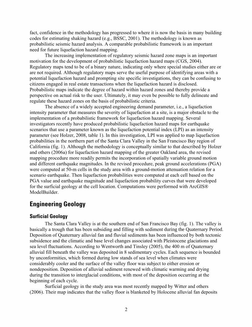
Surficial Geology The Santa Clara Valley is at the southern end of San Francisco Bay (fig. 1). The valley is

basically a trough that has been subsiding and filling with sediment during the Quaternary Period. Deposition of Quaternary alluvial fan and fluvial sediments has been influenced by both tectonic subsidence and the climatic and base level changes associated with Pleistocene glaciations and sea level fluctuations. According to Wentworth and Tinsley (2005), the 400 m of Quaternary alluvial fill beneath the valley was deposited in 8 sedimentary cycles. Each sequence is bounded by unconformities, which formed during low stands of sea level when climates were considerably cooler and the surface of the valley floor was subject to either erosion or nondeposition. Deposition of alluvial sediment renewed with climatic warming and drying during the transition to interglacial conditions, with most of the deposition occurring at the beginning of each cycle.

Surficial geology in the study area was most recently mapped by Witter and others (2006). Their map indicates that the valley floor is blanketed by Holocene alluvial fan deposits

2

(fig. 2). On the basis of the subsurface exploration conducted for this investigation, these deposits have an average thickness in the central part of the study area of ~9 m. Their maximum thickness is ~18 m. They thin outward from the axis of the valley. These Holocene sediments were deposited after the last glacial epoch and are the most recent sedimentary cycle described by Wentworth and Tinsley (2005). Pleistocene alluvial fan deposits from earlier cycles underlie these Holocene sediments and crop out along the margins of the valley.

The surficial geology shown in figure 2 is simplified from the mapping by Witter and others (2006) to emphasize the major units that were considered in the liquefaction hazard mapping. The map also shows locations of cone penetration test (CPT) soundings that were used to characterize the liquefaction hazard. Penetration data for these soundings are available at the USGS Earthquake Program web site (http://earthquake.usgs.gov/regional/nca/cpt/index.php). Witter and others (2006) identified three major Holocene fan facies or units: Qhfy, a coarser grained facies around the margin of the valley associated with the heads of the alluvial fans; Qhff, a finer grained facies that is the distal end of the fans; and Qhly/Qhl, levee deposits along modern creeks. The areas mapped as levee deposits presumably also include buried older Holocene channel and point bar deposits. In addition, Witter and others (2006) mapped a large area around the margin of San Francisco Bay that is underlain by estuarine deposits, Qhbm. This area was not explored for hazard mapping purposes because it was mostly inaccessible to the CPT truck that was used for the subsurface exploration. Urban development is modest in this area. The simplified map in figure 2 also does not distinguish among Pleistocene alluvial fan deposits mapped by Witter and others (2006). These deposits are identified here simply as Qpf.

The original surficial geologic map identified 18 Holocene surficial units, including many on the valley floor that were of limited extent (Witter and others, 2006). It was not practical to explore systematically these minor units with the CPT because of site access limitations. To make the liquefaction hazard map, the minor units were grouped with the major unit with which we anticipated they would have the greatest similarity based on the geologic descriptions by Witter and others (2006). The impact on the appearance of the resulting hazard map is modest.

Earthquake Potential The Santa Clara Valley is bounded by two active strike-slip fault systems that are the

principal components of the transform boundary between the Pacific and North American tectonic plates in the Bay area (fig. 1). The San Andreas Fault lies to the west of the study area. It generated the 1906 M7.8 San Francisco earthquake, which ruptured 470 km of the fault. An earthquake like the 1906 event is the largest earthquake that is expected to shake the study area (WGCEP, 2003). The Hayward and Calaveras Faults lie to the east. The largest historical earthquake on these faults was the 1868 M~6.7 Hayward earthquake. Both the 1868 and 1906 earthquakes caused liquefaction in the study area (figs. 2 and 3). Reported liquefaction effects were confined to areas underlain by Latest Holocene alluvial fan levee deposits (Qhly) (fig. 2). The only other large historical earthquake, the 1989 M6.9 Loma Prieta earthquake which ruptured the southern segment of the 1906 San Andreas Fault rupture, did not cause liquefaction in the study area (Holzer, 1998).

Three earthquake scenarios were considered in this investigation, the two historical events described above, and a Calaveras Fault event. The likelihood of each of these events was evaluated by a USGS Working Group as part of an intensive investigation of potential earthquakes in the San Francisco Bay area (WGCEP, 2003). The group concluded that the 30-

3

year (2002-2031) probability is 0.05 for a repeat of the 1906 earthquake. The group also concluded that the 30-year probability is 0.11 for a repeat of the 1868 Hayward earthquake, which ruptured the southern segment of the fault. The southern segment is the closest portion of the Hayward Fault to the study area. The higher probability of the earthquake on the southern segment of the Hayward Fault relative to a 1906-like San Andreas Fault event is attributable to its smaller magnitude and the longer period of elapsed time, which has allowed tectonic strain to accumulate. The seismic potential of the Calaveras Fault is poorly known. The 1984 M6.2 Morgan Hill earthquake is the largest historical earthquake on the fault. The Working Group estimated that a rupture of the central and northern segments of the Calaveras Fault would produce an M6.9 earthquake, but the 30-year probability of the event is very low, 0.003. The study area is adjacent to the central segment of the Calaveras Fault.

Methodology

Liquefaction Prediction In this investigation, as in our earlier mapping efforts (Holzer and others, 2006a), LPI as

defined by Iwasaki and others (1978) was used to characterize the liquefaction hazard. Other definitions have been proposed, but redefining LPI can change the significance and interpretation of specific LPI values (Holzer, 2008). As proposed by Iwasaki and others (1978), LPI weighs liquefaction factors of safety and thickness of potentially liquefiable layers according to depth. It assumes that the severity of liquefaction is proportional to:

1. cumulative thickness of the liquefied layers; 2. proximity of liquefied layers to the surface; and 3. amount by which the liquefaction factor safety (FS) is less than 1.0, where FS is the

ratio of the soil capacity to resist liquefaction to seismic demand imposed by the earthquake.

Iwasaki and others (1978) defined LPI as:

∫=m

dzzwFLPI20

0

)( (1)

where F = 1 – FS for FS ≤ 1 (2a) F = 0 for FS > 1 (2b) w(z) = 10 – 0.5 z, where z is the depth in meters. (2c)

The weighting factor, w(z) ranges from ten at the surface to zero at 20 m (Iwasaki and others, 1978). F=0 above the water table. LPI values can theoretically range from 0 to 100.

FS in this investigation was computed with the Seed-Idriss simplified procedure (Seed and others, 1985) as modified for the CPT by Robertson and Wride (1998). This is the procedure recommended by Youd and others (2001). This methodology is consistent with the calibration of LPI by Toprak and Holzer (2003), which relied on Robertson and Wride (1998) to compute FS. Toprak and Holzer (2003) evaluated the significance of LPI values by correlating LPI with surface manifestations of liquefaction. They observed that the median values of LPI were 5 and

4

12, respectively, in areas with sand boils and lateral spreads. Lower and upper quartiles were 3 and 10 for sand boils and 5 and 17 for lateral spreads.

The advantage for hazard mapping of LPI over the simplified procedure is that it predicts the liquefaction hazard of the entire soil column at a specific location. The simplified procedure only predicts liquefaction potential of a soil element. By combining all of the factors of safety from a boring or sounding into a single value, LPI provides a spatially distributed parameter when multiple borings or soundings are conducted in a deposit.

The probability of surface manifestations of liquefaction for each surficial geologic unit was derived from complementary cumulative frequency distributions of LPI. Distributions were computed for a specific earthquake magnitude and water table condition. By computing distributions for different PGA values, probability as a function of PGA can be estimated for each unit based on the frequency at LPI ≥ 5. The procedure is illustrated in figure 4. Figure 4a shows LPI distributions of Latest Holocene alluvial fan levee deposits (Qhly) in the Santa Clara Valley assuming a 5-m-deep water table and a M7.0 earthquake. Each distribution is based on a specific PGA and the same 25 CPT soundings conducted in Qhly. The probability of liquefaction at each PGA is the frequency value at LPI≥ 5 for each distribution. Figure 4b shows the liquefaction probability as a function of PGA for an M7.0 earthquake. The probabilities were inferred from the frequency at LPI≥ 5 shown in figure 4a. This methodology is the same as that used to map liquefaction hazard in the greater Oakland area (Holzer and others, 2002; Holzer and others, 2006a; Holzer and others, 2006b). Although the complementary cumulative frequency at LPI≥ 5 is interpreted here as the conditional probability of liquefaction at a randomly selected location within the area underlain by the geologic unit given an earthquake magnitude and PGA, it also can be interpreted as the percent area with surface manifestations of liquefaction (Holzer and others, 2006a).

Predicting the probability of liquefaction with spatially variable ground motions can be computationally simplified by curve fitting the relation between probability and PGA. Holzer and others (2006b) recommended a 3-parameter logistic equation of the form shown in figure 4b. Rix and Romero-Hudock (2007) generalized the probability relation to other earthquake magnitudes by scaling the seismic demand (PGA) by the magnitude scaling factor (MSF) from the simplified procedure (fig. 4c). Data points in figure 4c are probabilities from complementary cumulative frequency distributions computed for 5.5≤M≤8.0 in 0.5 magnitude increments and 0≤PGA≤0.6g in 0.1g increments. In the simplified procedure as described in Youd and others (2001), MSF = 102.24/M2.56. Holzer (2008) recommended that the relation between liquefaction probability and magnitude-scaled PGA for a surficial geologic unit be referred to as the “liquefaction probability curve.”

The Robertson and Wride (1998) simplified procedure does not require soil samples for liquefaction evaluation. This is a convenient advantage when dealing with large numbers of CPT soundings as was the situation in this investigation. The procedure uses the soil behavior index, IC, to predict soil behavior. IC values are determined with the normalized and dimensionless cone tip resistance and friction ratio using equation (3).

IC = [(3.47 - log Q)2 + (1.22 + Log F)2]0.5 (3)

where Q = normalized tip resistance, dimensionless

5

F = normalized friction ratio, dimensionless. For details of the normalization and nondimensionalization, the reader is referred to

Robertson and Wride (1998). Values of IC range from 1.64 or less for clean sands to values greater than 2.6 for silt mixtures and finer grained soils. Soils with IC > 2.6 are not considered to be susceptible to liquefaction. In the procedure as implemented by Robertson and Wride (1998), an apparent fines correction based on IC value is applied for soils with 1.64 < IC < 2.6.

On the basis of both the geologic setting inferred from CPT profiles in the Santa Clara Valley and experience during hazard mapping of geologically similar deposits in greater Oakland (Holzer and others, 2006a), we were concerned that nonsusceptible fine-grained soils in the alluvial fan deposits soils with IC values near but slightly less than 2.6 were being incorrectly classified as susceptible to liquefaction. This concern was greatest at sites with thick accumulations of fine-grained Holocene flood overbank deposits where IC values varied around 2.6. Depth intervals with IC values just slightly less than 2.6 at some of these sites contributed significantly to LPI values. To evaluate the capability of IC to correctly classify the susceptibility of these fine-grained soils in the Santa Clara Valley, samples were collected adjacent to 6 soundings in geologic units Qhff, Qhf, and Qhl. Only a few sites were sampled because of challenges of permitting, but the selected sites were believed to be generally representative of surficial geologic units.

Soil samples collected at these sites indicated that the soil behavior index misclassified these fine-grained soils as susceptible to liquefaction. Geotechnical tests on these samples indicated the soil was not susceptible. This is illustrated in figure 5, which compares the penetration profile for CPT SCC008 with geotechnical properties of soil samples from an adjacent 5-m-deep boring. The sounding and adjacent boring were conducted in Qhff, the fine grained alluvial fan facies. The SCC008 CPT profile encountered an 8-m thick Holocene flood overbank deposit with an IC≈ 2.6. Although the Robertson-Wride procedure predicts FS<1 in the parts of the interval where IC values are slightly less than 2.6, soil from the sampled depth interval, 0 to 5 m, is not susceptible to liquefaction according to criteria published by Idriss and Boulanger (2006) and Bray and Sancio (2006). The plasticity indices of the soil samples are generally greater than 12 and clay (<5 μ) percentage ranges from 30 to 60 %. The soil in the 8-m interval is a lean to fat clay (CL-CH in the Unified Soil Classification System).

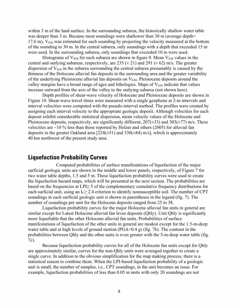
The manner in which Robertson and Wride (1998) automated their procedure is a significant cause of the misclassification problem for Santa Clara Valley soils. Figure 6 shows the original Robertson (1990) soil behavior type classification chart. The chart divides soil behavior types into 9 zones. Most of the F and Q values for the sampled intervals from SCC008 plot in zone 4 (see plus symbols in figure 6), which are nonsusceptible silt mixtures according to Robertson and Wride (1998). In order to automate the classification, Robertson and Wride (1998) approximated the zone boundaries on the original chart with circles of constant I defined by equation (3). They approximated the boundary between zones 4 (silt mixtures) and 5 (sand mixtures) on the original chart by a circle with an I = 2.6. As is seen in figure 6, equation (3) poorly approximates the boundary between zones 4 and 5 at normalized dimensionless friction ratios greater than 2, which is where most of the sampled depth intervals from SCC008 plot. Despite correctly plotting in zone 4, the I values for soils in the sampled interval are only

C

C

C slightly less than 2.6. Thus, most of the soil with IC < 2.6 is misclassified by the automated procedure as susceptible sand mixtures rather than nonsusceptible silt mixtures.

6

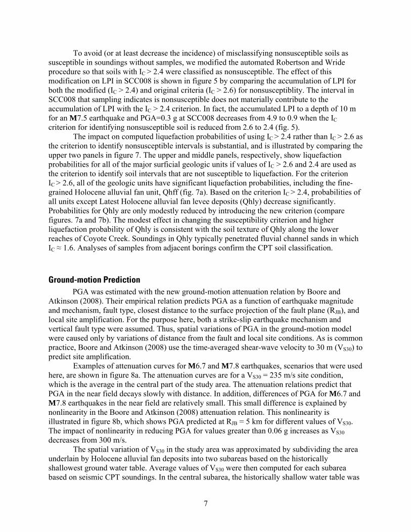
To avoid (or at least decrease the incidence) of misclassifying nonsusceptible soils as susceptible in soundings without samples, we modified the automated Robertson and Wride procedure so that soils with IC > 2.4 were classified as nonsusceptible. The effect of this modification on LPI in SCC008 is shown in figure 5 by comparing the accumulation of LPI for both the modified (IC > 2.4) and original criteria (IC > 2.6) for nonsusceptiblity. The interval in SCC008 that sampling indicates is nonsusceptible does not materially contribute to the accumulation of LPI with the IC > 2.4 criterion. In fact, the accumulated LPI to a depth of 10 m for an M7.5 earthquake and PGA=0.3 g at SCC008 decreases from 4.9 to 0.9 when the IC criterion for identifying nonsusceptible soil is reduced from 2.6 to 2.4 (fig. 5).

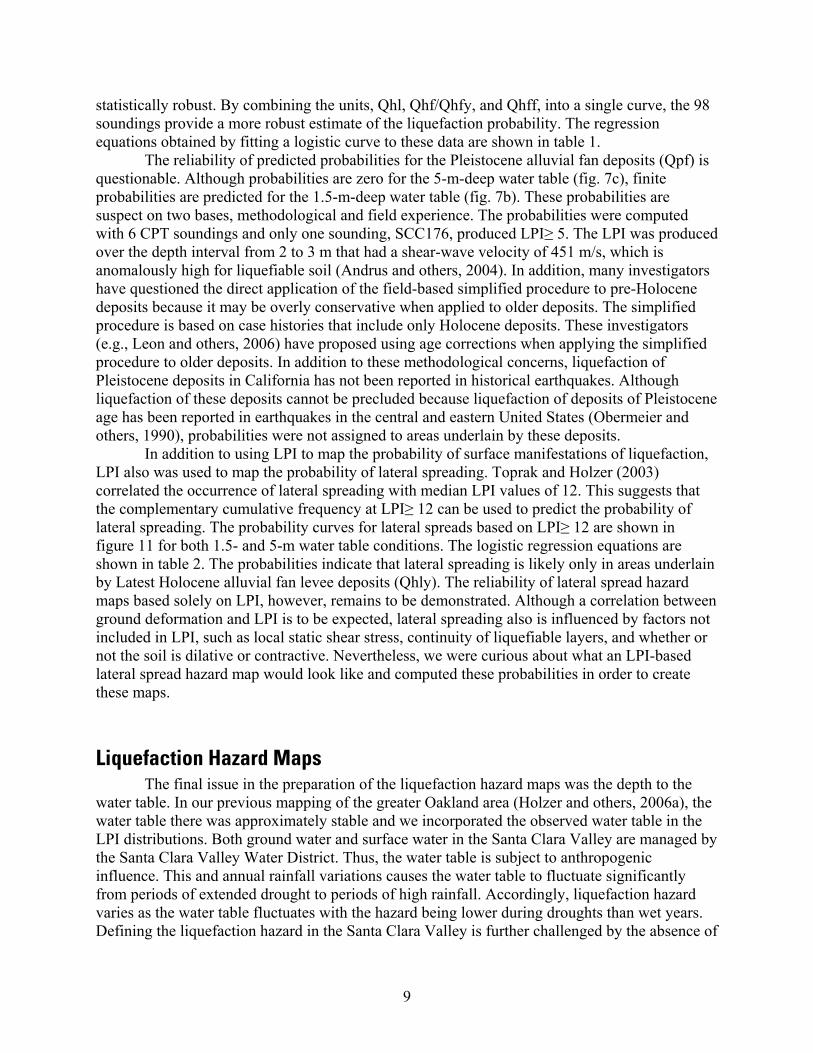
The impact on computed liquefaction probabilities of using IC > 2.4 rather than IC > 2.6 as the criterion to identify nonsusceptible intervals is substantial, and is illustrated by comparing the upper two panels in figure 7. The upper and middle panels, respectively, show liquefaction probabilities for all of the major surficial geologic units if values of IC > 2.6 and 2.4 are used as the criterion to identify soil intervals that are not susceptible to liquefaction. For the criterion IC > 2.6, all of the geologic units have significant liquefaction probabilities, including the fine-grained Holocene alluvial fan unit, Qhff (fig. 7a). Based on the criterion IC > 2.4, probabilities of all units except Latest Holocene alluvial fan levee deposits (Qhly) decrease significantly. Probabilities for Qhly are only modestly reduced by introducing the new criterion (compare figures. 7a and 7b). The modest effect in changing the susceptibility criterion and higher liquefaction probability of Qhly is consistent with the soil texture of Qhly along the lower reaches of Coyote Creek. Soundings in Qhly typically penetrated fluvial channel sands in which IC ≈ 1.6. Analyses of samples from adjacent borings confirm the CPT soil classification.

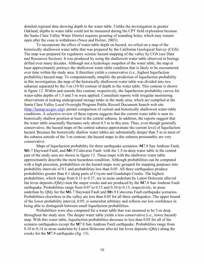
Ground-motion Prediction PGA was estimated with the new ground-motion attenuation relation by Boore and Atkinson (2008). Their empirical relation predicts PGA as a function of earthquake magnitude and mechanism, fault type, closest distance to the surface projection of the fault plane (R ), and local site amplification. For the purpose here, both a strike-slip earthquake mechanism and vertical fault type were assumed. Thus, spatial variations of PGA in the ground-motion model were caused only by variations of distance from the fault and local site conditions. As is common practice, Boore and Atkinson (2008) use the time-averaged shear-wave velocity to 30 m (V ) to predict site amplification

JB

S30.

Examples of attenuation curves for M6.7 and M7.8 earthquakes, scenarios that were used here, are shown in figure 8a. The attenuation curves are for a VS30 = 235 m/s site condition, which is the average in the central part of the study area. The attenuation relations predict that PGA in the near field decays slowly with distance. In addition, differences of PGA for M6.7 and M7.8 earthquakes in the near field are relatively small. This small difference is explained by nonlinearity in the Boore and Atkinson (2008) attenuation relation. This nonlinearity is illustrated in figure 8b, which shows PGA predicted at RJB = 5 km for different values of VS30. The impact of nonlinearity in reducing PGA for values greater than 0.06 g increases as VS30 decreases from 300 m/s.

The spatial variation of VS30 in the study area was approximated by subdividing the area underlain by Holocene alluvial fan deposits into two subareas based on the historically shallowest ground water table. Average values of VS30 were then computed for each subarea based on seismic CPT soundings. In the central subarea, the historically shallow water table was

7

within 3 m of the land surface. In the surrounding subarea, the historically shallow water table was deeper than 3 m. Because most soundings were shallower than 30 m (average depth= 17.6 m), VS30 was estimated for each sounding by projecting the velocity measured at the bottom of the sounding to 30 m. In the central subarea, only soundings with a depth that exceeded 15 m were used. In the surrounding subarea, only soundings that exceeded 10 m were used.

Histograms of VS30 for each subarea are shown in figure 9. Mean VS30 values in the central and outlying subareas, respectively, are 235 (± 21) and 291 (± 62) m/s. The greater dispersion of VS30 in the subarea surrounding the central subarea presumably is caused by the thinness of the Holocene alluvial fan deposits in the surrounding area and the greater variability of the underlying Pleistocene alluvial fan deposits on VS30. Pleistocene deposits around the valley margins have a broad range of ages and lithologies. Maps of VS30 indicate that values increase outward from the axis of the valley to the outlying subarea (not shown here).

Depth profiles of shear-wave velocity of Holocene and Pleistocene deposits are shown in Figure 10. Shear-wave travel times were measured with a single geophone at 2-m intervals and interval velocities were computed with the pseudo-interval method. The profiles were created by assigning each interval velocity to the appropriate geologic deposit. Although velocities for each deposit exhibit considerable statistical dispersion, mean velocity values of the Holocene and Pleistocene deposits, respectively, are significantly different, 207(±33) and 303(±77) m/s. These velocities are ~10 % less than those reported by Holzer and others (2005) for alluvial fan deposits in the greater Oakland area [224(±51) and 330(±84) m/s], which is approximately 40 km northwest of the present study area.

Liquefaction Probability Curves Computed probabilities of surface manifestations of liquefaction of the major

surficial geologic units are shown in the middle and lower panels, respectively, of Figure 7 for two water table depths, 1.5 and 5 m. These liquefaction probability curves were used to create the liquefaction hazard maps, which will be presented in the next section. The probabilities are based on the frequencies at LPI≥ 5 of the complementary cumulative frequency distributions for each surficial unit, using an IC≥ 2.4 criterion to identify nonsusceptible soil. The number of CPT soundings in each surficial geologic unit is shown in parentheses in the legend (fig. 7). The number of soundings per unit for the Holocene deposits ranged from 25 to 38.

Liquefaction probability curves for the major Holocene alluvial fan units in general are similar except for Latest Holocene alluvial fan levee deposits (Qhly). Unit Qhly is significantly more liquefiable that the other Holocene alluvial fan units. Probabilities of surface manifestations of liquefaction of the other units in general are modest except for the 1.5-m-deep water table and at high levels of ground motion (PGA>0.4 g) (fig. 7b). The contrast in the probabilities between Qhly and the other units is even greater with the 5-m-deep water table (fig. 7c).

Because liquefaction probability curves for all of the Holocene fan units except for Qhly are approximately similar, curves for the non-Qhly units were averaged together to create a single curve. In addition to the obvious simplification for the map making process, there is a statistical reason to combine them. When the LPI-based liquefaction probability of a geologic unit is small, the number of samples, i.e., CPT soundings, in the unit becomes an issue. For example, liquefaction probabilities of less than 0.05 in units with only 20 soundings are not

8

statistically robust. By combining the units, Qhl, Qhf/Qhfy, and Qhff, into a single curve, the 98 soundings provide a more robust estimate of the liquefaction probability. The regression equations obtained by fitting a logistic curve to these data are shown in table 1.

The reliability of predicted probabilities for the Pleistocene alluvial fan deposits (Qpf) is questionable. Although probabilities are zero for the 5-m-deep water table (fig. 7c), finite probabilities are predicted for the 1.5-m-deep water table (fig. 7b). These probabilities are suspect on two bases, methodological and field experience. The probabilities were computed with 6 CPT soundings and only one sounding, SCC176, produced LPI≥ 5. The LPI was produced over the depth interval from 2 to 3 m that had a shear-wave velocity of 451 m/s, which is anomalously high for liquefiable soil (Andrus and others, 2004). In addition, many investigators have questioned the direct application of the field-based simplified procedure to pre-Holocene deposits because it may be overly conservative when applied to older deposits. The simplified procedure is based on case histories that include only Holocene deposits. These investigators (e.g., Leon and others, 2006) have proposed using age corrections when applying the simplified procedure to older deposits. In addition to these methodological concerns, liquefaction of Pleistocene deposits in California has not been reported in historical earthquakes. Although liquefaction of these deposits cannot be precluded because liquefaction of deposits of Pleistocene age has been reported in earthquakes in the central and eastern United States (Obermeier and others, 1990), probabilities were not assigned to areas underlain by these deposits.

In addition to using LPI to map the probability of surface manifestations of liquefaction, LPI also was used to map the probability of lateral spreading. Toprak and Holzer (2003) correlated the occurrence of lateral spreading with median LPI values of 12. This suggests that the complementary cumulative frequency at LPI≥ 12 can be used to predict the probability of lateral spreading. The probability curves for lateral spreads based on LPI≥ 12 are shown in figure 11 for both 1.5- and 5-m water table conditions. The logistic regression equations are shown in table 2. The probabilities indicate that lateral spreading is likely only in areas underlain by Latest Holocene alluvial fan levee deposits (Qhly). The reliability of lateral spread hazard maps based solely on LPI, however, remains to be demonstrated. Although a correlation between ground deformation and LPI is to be expected, lateral spreading also is influenced by factors not included in LPI, such as local static shear stress, continuity of liquefiable layers, and whether or not the soil is dilative or contractive. Nevertheless, we were curious about what an LPI-based lateral spread hazard map would look like and computed these probabilities in order to create these maps.

Liquefaction Hazard Maps The final issue in the preparation of the liquefaction hazard maps was the depth to the

water table. In our previous mapping of the greater Oakland area (Holzer and others, 2006a), the water table there was approximately stable and we incorporated the observed water table in the LPI distributions. Both ground water and surface water in the Santa Clara Valley are managed by the Santa Clara Valley Water District. Thus, the water table is subject to anthropogenic influence. This and annual rainfall variations causes the water table to fluctuate significantly from periods of extended drought to periods of high rainfall. Accordingly, liquefaction hazard varies as the water table fluctuates with the hazard being lower during droughts than wet years. Defining the liquefaction hazard in the Santa Clara Valley is further challenged by the absence of

9

detailed regional data showing depth to the water table. Unlike the investigation in greater Oakland, depths to water table could not be measured during the CPT field exploration because the Santa Clara Valley Water District requires grouting of sounding holes, which may remain open after the cone is withdrawn (Noce and Holzer, 2003).

To incorporate the effect of water-table depth on hazard, we relied on a map of the historically shallowest water table that was prepared by the California Geological Survey (CGS). The map was prepared for regulatory seismic hazard mapping of the valley by CGS (see Data and Resources Section). It was produced by using the shallowest water table observed in borings drilled over many decades. Although not a hydrologic snapshot of the water table, the map at least approximately portrays the shallowest water table condition that is likely to be encountered over time within the study area. It therefore yields a conservative (i.e., highest liquefaction probability) hazard map. To computationally simplify the prediction of liquefaction probability in this investigation, the map of the historically shallowest water table was divided into two subareas separated by the 3-m (10-ft) contour of depth to the water table. This contour is shown in figure 12. Within and outside this contour, respectively, the liquefaction probability curves for water-table depths of 1.5 and 5 m were applied. Consultant reports with irregular monitoring observations at leaking underground storage tanks in the study area, which are compiled at the Santa Clara Valley Local Oversight Program Public Record Document Search web site (http://lustop.sccgov.org), permit comparison of current and historically shallowest water-table conditions. A selective review of these reports suggests that the current water table is near its historically shallow position at least in the central subarea. In addition, the reports suggest that the water table seasonally fluctuates only about 0.5 m in this area. Thus, even though generally conservative, the hazard maps of the central subarea approximate the current level of liquefaction hazard. Because the historically shallow water tables are substantially deeper than 5 m in most of the subarea outside of the 3-m contour, the hazard maps in this subarea presumably are very conservative.

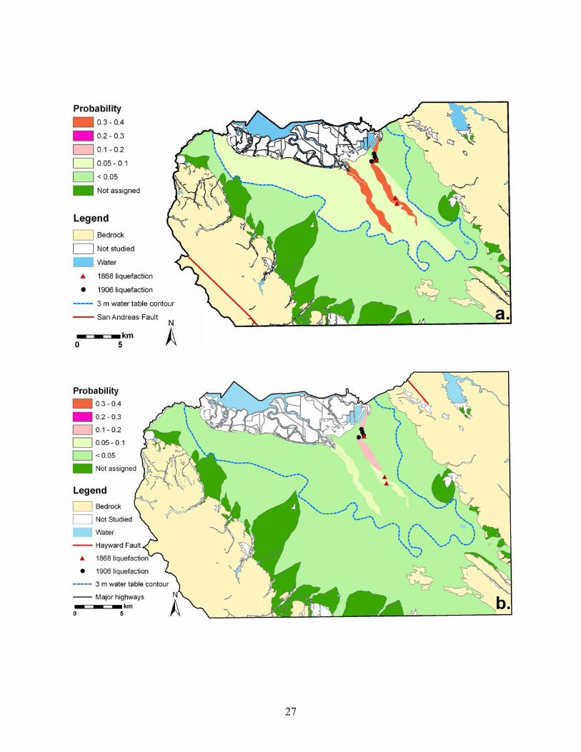
Maps of liquefaction probability for three earthquake scenarios–M7.8 San Andreas Fault, M6.7 Hayward Fault, and M6.9 Calaveras Fault–with the 1.5-m-deep water table in the central part of the study area are shown in figure 12. These maps with the shallower water table approximately describe the most hazardous condition. Although probabilities can be computed with a high precision, probabilities on the hazard maps were grouped for mapping purposes into probability intervals of 0.1 and probabilities less than 0.05. All three earthquakes produce probabilities greater than 0.1 along parts of Coyote and Guadalupe Creeks. The highest probabilities, which range from 0.33 to 0.37, are in areas underlain by Latest Holocene alluvial fan levee deposits (Qhly) near the major creeks and are produced by the M7.8 San Andreas Fault earthquake. Probabilities range from 0.07 to 0.15 and 0.10 to 0.13, respectively, in areas underlain by Qhly for the M6.7 Hayward Fault and M6.9 Calaveras Fault earthquake scenarios. Probabilities elsewhere in the valley are less than 0.05 for all three earthquakes. The upper bound of the lower probability interval, 0.05, is somewhat arbitrary and reflects our low confidence in being able to distinguish between small liquefaction probabilities.

Probabilities were also computed for a water table that was assumed to be 5-m deep throughout the study area. The deeper water table yields a less conservative (i.e., lower hazard) map. With this water table, liquefaction probabilities decrease to less than 0.05 for all of the scenario earthquakes except the M7.8 San Andreas Fault earthquake. Probabilities range from 0.10 to 0.14 in areas underlain by Latest Holocene alluvial fan levee deposits (Qhly) along the creeks for the M7.8 earthquake (fig. 13).

10

Figure 14 illustrates a lateral spread hazard map based on LPI. The probability of lateral spreading is based on the LPI≥ 12 criterion (fig. 11). The probability of lateral spreading is locally greater than 0.05 for only the M7.8 San Andreas Fault earthquake scenario with the shallow 1.5-m-deep water table (fig. 14). Probabilities range from 0.06 to 0.09 in areas underlain by Latest Holocene alluvial fan levee deposits (Qhly) along the creeks for this earthquake and the shallow water table. Probabilities of lateral spreading are less than 0.01 for all of the other earthquake scenarios as well as the M7.8 San Andreas Fault earthquake scenario when the water table is assumed to be 5-m deep.

Discussion Although a rigorous test of the mapped predictions in the study area with observations of

liquefaction in historical earthquakes is not possible, a qualitative comparison with observations during the 1868 Hayward Fault and 1906 San Francisco earthquakes is possible. In addition, the absence of liquefaction during the 1989 M6.9 Loma Prieta earthquake can be used to evaluate the methodology.

Both Lawson (1908) and Youd and Hoose (1978) reported extensive ground failure along Coyote Creek that indicates liquefaction was widespread in both the 1868 and 1906 earthquakes. Descriptions include sand boils, settlements, and lateral spreading. Some of the descriptions are confirmed with photographs (e.g., fig. 3), which leaves little doubt about the nature of the mechanism of ground failure. Although Lawson (1908) did not map these occurrences, descriptions of landmarks and references to property ownership where effects were observed permit fairly accurate locations of many observations (Youd and Hoose, 1978). In addition to these descriptions, Youd and Hoose (1978) added accounts from newspapers. We reviewed these locations and plotted them on the geologic map (fig. 2) and the liquefaction hazard maps. All of the liquefaction reports are located in the area underlain by Latest Holocene alluvial fan levee deposits (Qhly), the unit with the highest liquefaction probability. No liquefaction appears to be associated with the other Holocene units. This is consistent with the observation by Youd and Hoose (1978, p. 23) that “no significant failures were reported on late Pleistocene and most Holocene alluvial fan deposits at points well removed from active stream channels.”

Although it would be helpful for assessing the reliability of the hazard maps if the percent of the area underlain by Latest Holocene alluvial fan levee deposits (Qhly) that liquefied in 1906 could be estimated, descriptions compiled by Lawson (1908) and Youd and Hoose (1978) do not permit this assessment. Nevertheless, their descriptions clearly indicate that liquefaction was extensive along and near Coyote Creek. These descriptions are generally consistent with the maps in figures 12 and 13. For the shallower water table condition, the percentage of area underlain by Qhly that is predicted to exhibit surface manifestations of liquefaction in 1868 and 1906, respectively, ranged from 7 to 15 % and 33 to 37 %. For the deeper water table, only the 1906 earthquake yielded areal estimates greater than 5, ranging from 10 to 14 %. Depths to the water table are unknown during both of these historical earthquakes, although the water table was probably shallower during the 1906 earthquake than during the 1868 earthquake. The former earthquake occurred in April near the end of the rainy season, and the latter earthquake occurred in October near the end of dry season.

Liquefaction probabilities (not shown) were also computed for the 1989 M6.9 Loma Prieta earthquake, which ruptured a segment of the San Andreas Fault south of the study area. As

11

noted previously, surface effects of liquefaction were not observed in 1989 (Holzer, 1998). Computed liquefaction probabilities in Latest Holocene alluvial fan levee deposits (Qhly) for the 1989 earthquake were less than 0.02 for the 5-m-deep water-table condition. The Loma Prieta earthquake occurred on October 17 near the end of the dry season when water tables typically are deepest.

The liquefaction hazard maps for the northern Santa Clara Valley highlight the need for meaningful observations of depth to the water table. Without such information, the accuracy of the hazard map is compromised. This issue of water table depth is further complicated in the Santa Clara Valley because of the conjunctive management of ground and surface water. This causes the hazard to vary secularly depending on climatic conditions. The impact of the position of the water table on liquefaction probability is illustrated in figure 15, which shows liquefaction probability curves for Latest Holocene alluvial fan levee deposits (Qhly) for different water table depths. Probabilities decay approximately monotonically to zero when the water table reaches a depth of ~9 m. This corresponds to the average thickness of Qhly in the central subarea, which implies that the saturated thickness of Qhly is critical in determining the liquefaction hazard.

The adoption in this investigation of IC > 2.4 as the criterion to identify soils that are not susceptible to liquefaction significantly reduced the probabilities of liquefaction for all of the surficial geologic units but Latest Holocene alluvial fan levee deposits (Qhly). Although we are not prepared to recommend a basic change in the Robertson and Wride (1998) procedure to incorporate this criterion, three considerations justified its adoption in the present investigation. First, sampled nonsusceptible soils in the Santa Clara Valley plot in zone 4 on Roberton’s (1990) original soil behavior type chart. This zone includes nonsusceptible silt mixtures. An IC equal to 2.4 rather 2.6 better approximates the soil behavior type boundary between zones 4 and 5 where F > 2, and thereby properly classifies these soils. Second, the modified criterion is consistent with the synthesis of CPT observations at 78 sites in Japan where liquefaction is known either to have or not to have occurred during earthquakes (Suzuki and others, 2003). They reported no liquefaction where IC > 2.4. And third, the probability curves based on an IC>2.4 criterion reasonably predict the observed patterns of liquefaction in this investigation. If the original IC > 2.6 criterion had been applied, significant liquefaction would have been predicted in the alluvial fan areas where no historical liquefaction has been reported.

Liquefaction probabilities predicted for Qpf, although not statistically robust because of the small number of soundings, highlight an ongoing issue with the application of the simplified procedure to soils that predate the Holocene Epoch. As previously noted, the straightforward application of the procedure to these older soils has been challenged by multiple investigators because it appears to underestimate their liquefaction resistance. This shortcoming and the absence of reports of liquefaction associated with Pleistocene deposits in historical California earthquakes prompted us not to assign probabilities predicted with the simplified procedure to areas underlain by these older deposits. Liquefaction of Pleistocene deposits, however, has been reported in several non-California earthquakes in the United States. It was observed in both late Pleistocene valley train deposits during the 1811-12 New Madrid, Missouri, earthquakes and Pleistocene beach ridges during the 1886 Charleston, South Carolina, earthquake (Obermeier and others, 1990). Improving the reliability of the simplified procedure for predicting the liquefaction potential of Pleistocene deposits is an important research need for liquefaction hazard mapping.

12

Acknowledgments Reviews by Ronald D. Andrus and John C. Tinsley, III, of an early draft of this

manuscript are appreciated. Raymond C. Wilson and Thomas M. Brocher read the final draft. We also thank George Cook for alerting us to the consulting reports with repeated water table observations.

13

References Cited Andrus, R.D., Stokoe, K.H., and Juang, C.H., 2004, Guide for shear-wave-based liquefaction

potential evaluation: Earthquake Spectra, v. 20, no. 2, p. 285-308. Boore, D.M., and Atkinson, G.M., 2008, Ground-motion prediction equations for the average

horizontal component of PGA, PGV, and 5 %-damped PSA at spectral periods between 0.01 s and 10.0 s: Earthquake Spectra, v. 24, no. 1, p. 99-138.

Bray, J.D., and Sancio, R.B., 2006, Assessment of the liquefaction susceptibility of fine-grained soils: Journal of Geotechnical and Geoenvironmental Engineering, v. 132, no. 9, p. 1165-1177.

BSSC, 2001, 2000 Edition NEHRP recommended provisions for seismic regulations for new buildings and other structures, FEMA 368, Part 1 (provisions): Federal Emergency Management Agency, 374 p.

CGS, 2004, Recommended criteria for delineating seismic hazard zones in California: California Division of Mines and Geology Special Publication 118, 12 p.

Cornell, C.A., 1968, Engineering seismic risk analysis: Seismological Society of America Bulletin, v. 58, no. 5, p. 1583-1606.

Holzer, T.L., ed., 1998, The Loma Prieta, California, earthquake of October 17, 1989 - Liquefaction, U. S. Geological Survey Professional Paper 1551-B, 314 p.

Holzer, T.L., 2008, Probabilistic liquefaction hazard mapping, in 4th Geotechnical Earthquake Engineering and Soil Dynamics, Sacramento, CA, May 18-22, 2008, American Society of Civil Engineers Geotechnical Special Publication 181, p.1-32.

Holzer, T.L., Bennett, M.J., Noce, T.E., Padovani, A.C., and Tinsley, J.C., III, 2002, Liquefaction hazard and shaking amplification maps of Alameda, Berkeley, Emeryville, Oakland, and Piedmont: A digital database: U.S. Geological Survey 02-296, http://pubs.usgs.gov/of/2002/02-296.

Holzer, T.L., Bennett, M.J., Noce, T.E., Padovani, A.C., and Tinsley, J.C., III, 2006a, Liquefaction hazard mapping with LPI in the greater Oakland, California, area: Earthquake Spectra, v. 22, no. 3, p. 693-708.

Holzer, T.L., Bennett, M.J., Noce, T.E., and Tinsley, J.C., III, 2005, Shear-wave velocity of surficial geologic sediments in Northern California: Statistical distributions and depth dependence: Earthquake Spectra, v. 21, no. 1, p. 161-177.

Holzer, T.L., Blair, J.L., Noce, T.E., and Bennett, M.J., 2006b, Predicted liquefaction of East Bay fills during a repeat of the 1906 San Francisco earthquake: Earthquake Spectra, v. 22, no. S2, p. S261-S278.

Idriss, I.M., and Boulanger, R.W., 2006, Semi-empirical procedures for evaluating liquefaction potential during earthquakes: Soil Dynamics and Earthquake Engineering, v. 26, no. 2-4, p. 115-130.

Iwasaki, T., Tatsuoka, F., Tokida, K.-i., and Yasuda, S., 1978, A practical method for assessing soil liquefaction potential based on case studies at various sites in Japan, in 2nd International conference on microzonation, San Francisco, p. 885-896.

Lawson, A.C., ed., 1908, The California Earthquake of April 18, 1906: Report of the State Earthquake Investigation Commission: Washington, D.C., Carnegie Institution of Washington, Publication no. 87, v. 1, 451 p.

14

Leon, E., Gassman, S.L., and Talwani, P., 2006, Accounting for soil aging when assessing liquefaction potential: Journal of Geotechnical and Geoenvironmental Engineering, v. 132, no. 3, p. 363-377.

McGuire, R.K., 2004, Seismic hazard and risk analysis, Earthquake Engineering Research Institute, Monograph no. 10, 221 p.

Noce, T.E., and Holzer, T.L., 2003, CPT-hole closure: Ground water monitoring & remediation, v. 23, no. 1, p. 93-96.

Obermeier, S.F., Jacobson, R., Smoot, J., Weems, R.E., Gohn, G.S., Monroe, J.E., and Powars, D.S., 1990, Earthquake-induced liquefaction features in the coastal setting of South Carolina and in the fluvial setting of the New Madrid seismic zone: U.S. Geological Survey Professional Paper 1504, 44 p.

Rix, G.J., and Romero-Hudock. S., 2007, Liquefaction potential mapping in Memphis and Shel-by County, Tennessee, Unpublished Report to the U.S. Geological Survey, Denver, CO, 27 p., http://earthquake.usgs.gov/regional/ceus/products/download/Memphis_LPI.pdf.

Robertson, P.K., 1990, Soil classification using the CPT: Canadian Geotechnical Journal, v. 27, no. 1, p.151-158.

Robertson, P.K., and Wride (Fear), C.E., 1998, Evaluating cyclic liquefaction potential using the cone penetration test: Canadian Geotechnical Journal, v. 35, no. 3, p. 442-459.

Seed, H.B., and Idriss, I.M., 1982, Ground motions and soil liquefaction during earthquakes, Earthquake Engineering Research Institute, Monograph no. 5, 134 p.

Seed, H.B., Tokimatsu, K., Harder, L.F., and Chung, R.M., 1985, Influence of SPT procedures in soil liquefaction resistance evaluations: Journal of Geotechnical Engineering, v. 111, no. 12, p. 1425-1445.

Toprak, S., and Holzer, T.L., 2003, Liquefaction potential index: Field assessment: Journal of Geotechnical and Geoenvironmental Engineering, v. 129, no. 4, p. 315-322.

Toprak, S., Holzer, T.L., Bennett, M.J., and Tinsley, J.C., III, , 1999, CPT- and SPT-based probabilistic assessments of liquefaction potential, in Seventh U.S.-Japan workshop on earthquake resistant design of lifeline facilities and countermeasures against liquefaction, Seattle, Multidisciplinary Center for Earthquake Engineering Technical Report MCEER-99-0019, p. 69-86.

Wentworth, C.M., and Tinsley, J.C., 2005, Tectonic subsidence and cyclic Quaternary deposition controlled by climate variation, Santa Clara Valley, California [abs.]: Geological Society of America, Abstracts with Programs, v. 37, no. 4, p. 59.

WGCEP, 2003, Earthquake probabilities in the San Francisco Bay region 2002-2032: U.S. Geological Survey Open-file Report 03-214, http://pubs.usgs.gov/of/2003/of03-214/.

Witter, R.C., Knudsen, K.L., Sowers, J.M., Wentworth, C.M., Koehler, R.D., and Randolph, C.E., 2006, Maps of Quaternary deposits and liquefaction susceptibility in the central San Francisco Bay region, California: U.S. Geological Survey Open-file Report 06-1037, http://pubs.usgs.gov/of/2006/1037/of06-1037_1c.pdf.

Youd, T.L., and Hoose, S.N., 1978, Historic ground failures in Northern California triggered by earthquakes, U.S. Geological Survey Professional Paper 993, 177 p.

Youd, T.L., Idriss, I.M., Andrus, R.D., Arango, I., Castro, G., Christian, J.T., Dobry, R., Finn, W.D.L., Harder, L.F., Jr., Hynes, M.E., Ishihara, K., Koester, J.P., Liao, S.S.C., Marcuson, W.F., III, Martin, G.R., Mitchell, J.K., Moriwaki, Y., Power, M.S., Robertson, P.K., Seed, R.B., and Stokoe, K.H., II, 2001, Liquefaction resistance of soils: Summary report from the 1996 NCEER and 1998 NCEER/NSF workshops on evaluation of

15

liquefaction resistance of soils: Journal of Geotechnical and Geoenvironmental Engineering, v. 127, no. 10, p. 817-833.

16

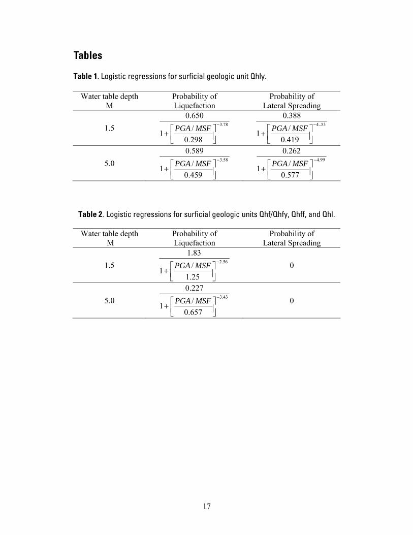
Tables Table 1. Logistic regressions for surficial geologic unit Qhly.

Water table depth M

Probability of Liquefaction

Probability of Lateral Spreading

1.5 78.3

298.0/1

650.0−

⎥⎦⎤

⎢⎣⎡+

MSFPGA 53..4

419.0/1

388.0−

⎥⎦⎤

⎢⎣⎡+

MSFPGA

5.0 58.3

459.0/1

589.0−

⎥⎦⎤

⎢⎣⎡+

MSFPGA 99.4

577.0/1

262.0−

⎥⎦⎤

⎢⎣⎡+

MSFPGA

Table 2. Logistic regressions for surficial geologic units Qhf/Qhfy, Qhff, and Qhl.

Water table depth M

Probability of Liquefaction

Probability of Lateral Spreading

1.5 56.2

25.1/1

83.1−

⎥⎦⎤

⎢⎣⎡+

MSFPGA

0

5.0 43.3

657.0/1

227.0−

⎥⎦⎤

⎢⎣⎡+

MSFPGA

0

17

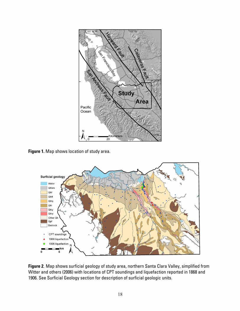
Figure 1. Map shows location of study area.

Figure 2. Map shows surficial geology of study area, northern Santa Clara Valley, simplified from Witter and others (2006) with locations of CPT soundings and liquefaction reported in 1868 and 1906. See Surficial Geology section for description of surficial geologic units.

18

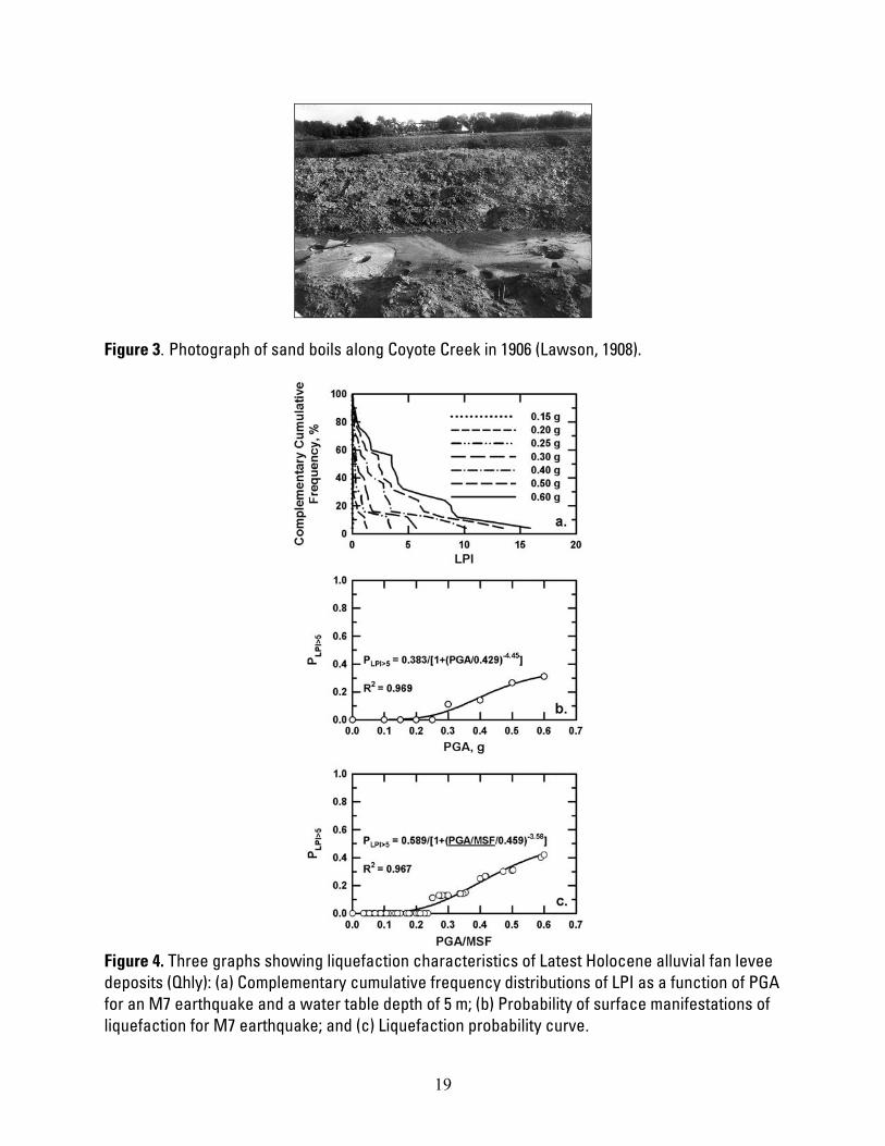
Figure 3. Photograph of sand boils along Coyote Creek in 1906 (Lawson, 1908).

Figure 4. Three graphs showing liquefaction characteristics of Latest Holocene alluvial fan levee deposits (Qhly): (a) Complementary cumulative frequency distributions of LPI as a function of PGA for an M7 earthquake and a water table depth of 5 m; (b) Probability of surface manifestations of liquefaction for M7 earthquake; and (c) Liquefaction probability curve.

19

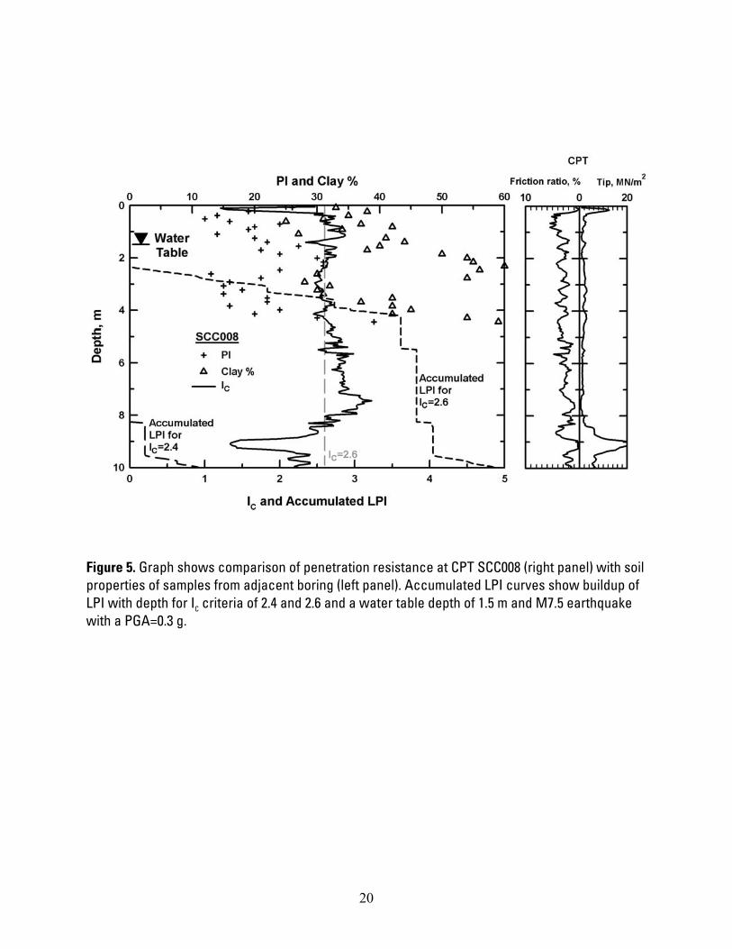
Figure 5. Graph shows comparison of penetration resistance at CPT SCC008 (right panel) with soil properties of samples from adjacent boring (left panel). Accumulated LPI curves show buildup of LPI with depth for I criteria of 2.4 and 2.6 and a water table depth of 1.5 m and M7.5 earthquake with a PGA=0.3 g.

C

20

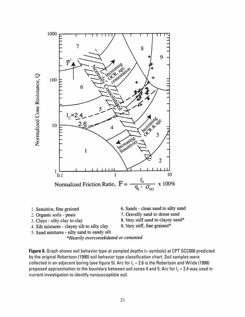
Figure 6. Graph shows soil behavior type at sampled depths (+ symbols) at CPT SCC008 predicted by the original Robertson (1990) soil behavior type classification chart. Soil samples were collected in an adjacent boring (see figure 5). Arc for I = 2.6 is the Robertson and Wride (1998) proposed approximation to the boundary between soil zones 4 and 5. Arc for I = 2.4 was used in current investigation to identify nonsusceptible soil.

C

C

21

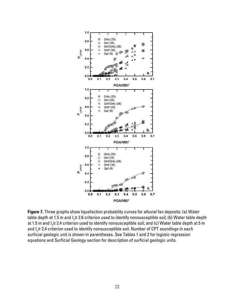
Figure 7. Three graphs show liquefaction probability curves for alluvial fan deposits: (a) Water table depth at 1.5 m and I ≥ 2.6 criterion used to identify nonsusceptible soil; (b) Water table depth at 1.5 m and I ≥ 2.4 criterion used to identify nonsusceptible soil; and (c) Water table depth at 5 m and I ≥ 2.4 criterion used to identify nonsusceptible soil. Number of CPT soundings in each surficial geologic unit is shown in parentheses. See Tables 1 and 2 for logistic regression equations and Surficial Geology section for description of surficial geologic units.

C

C

C

22

Figure 8. Two graphs show median ground motion predictions by Boore and Atkinson (2008): (a) PGA as a function of distance from fault (R ) for sites with V =235 m/s, and (b) PGA at 5 km as a function of V

JB S30

S30.

23

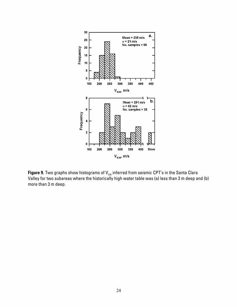
Figure 9. Two graphs show histograms of V inferred from seismic CPT’s in the Santa Clara Valley for two subareas where the historically high water table was (a) less than 3 m deep and (b) more than 3 m deep

S30

.

24

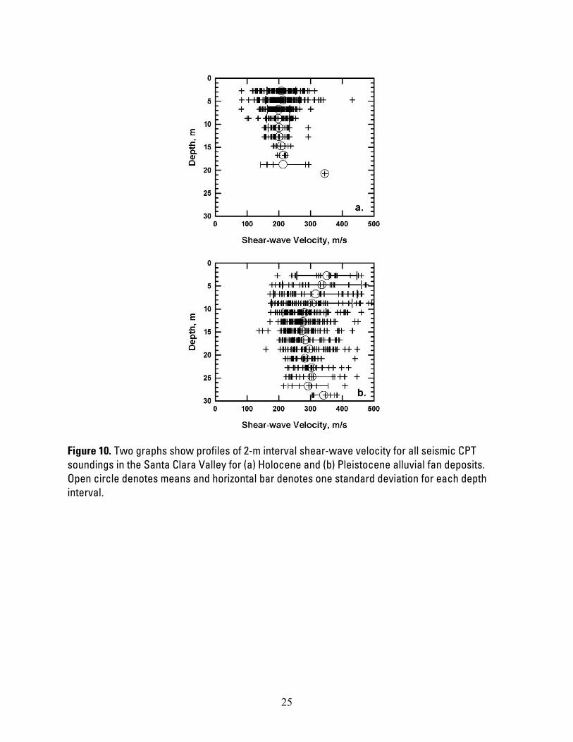
Figure 10. Two graphs show profiles of 2-m interval shear-wave velocity for all seismic CPT soundings in the Santa Clara Valley for (a) Holocene and (b) Pleistocene alluvial fan deposits. Open circle denotes means and horizontal bar denotes one standard deviation for each depth interval.

25

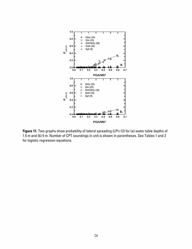
Figure 11. Two graphs show probability of lateral spreading (LPI>12) for (a) water table depths of 1.5 m and (b) 5 m. Number of CPT soundings in unit is shown in parentheses. See Tables 1 and 2 for logistic regression equations.

26

27

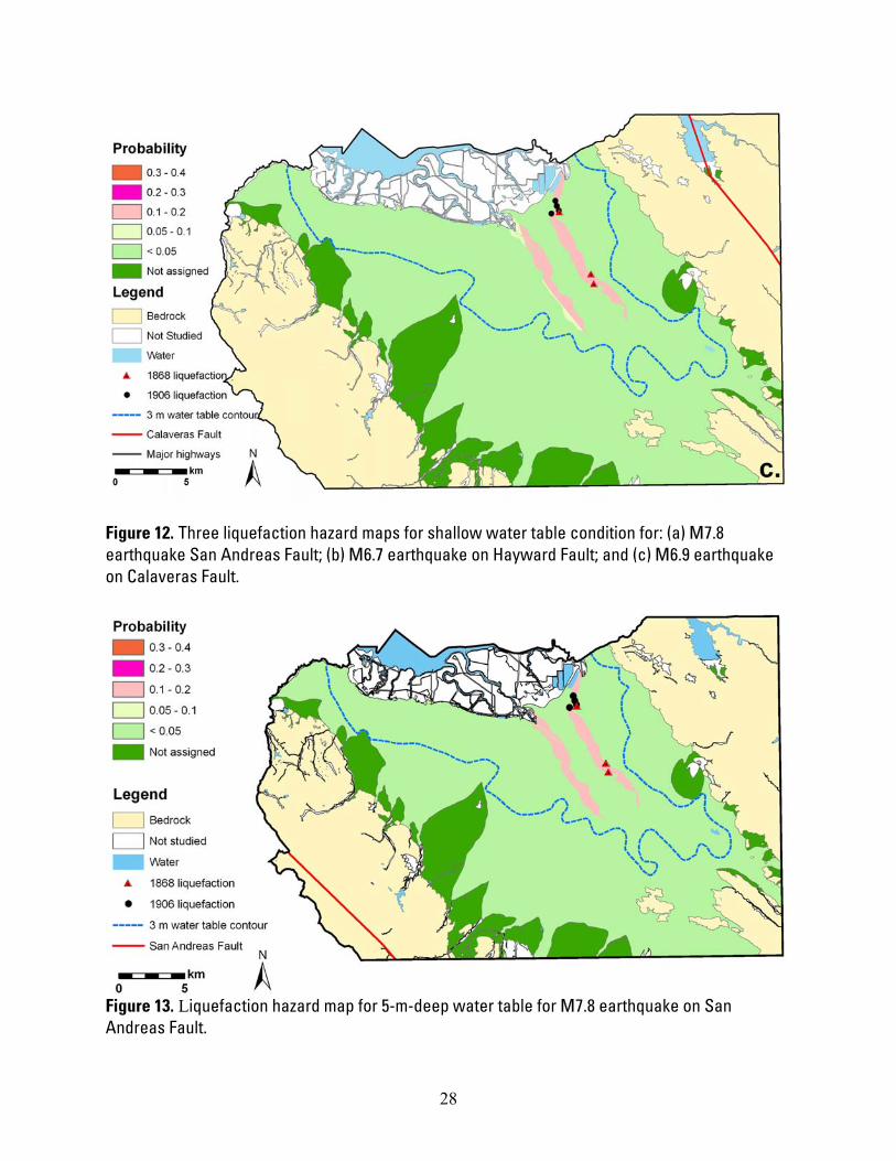
Figure 12. Three liquefaction hazard maps for shallow water table condition for: (a) M7.8 earthquake San Andreas Fault; (b) M6.7 earthquake on Hayward Fault; and (c) M6.9 earthquake on Calaveras Fault.

Figure 13. Liquefaction hazard map for 5-m-deep water table for M7.8 earthquake on San Andreas Fault.

28

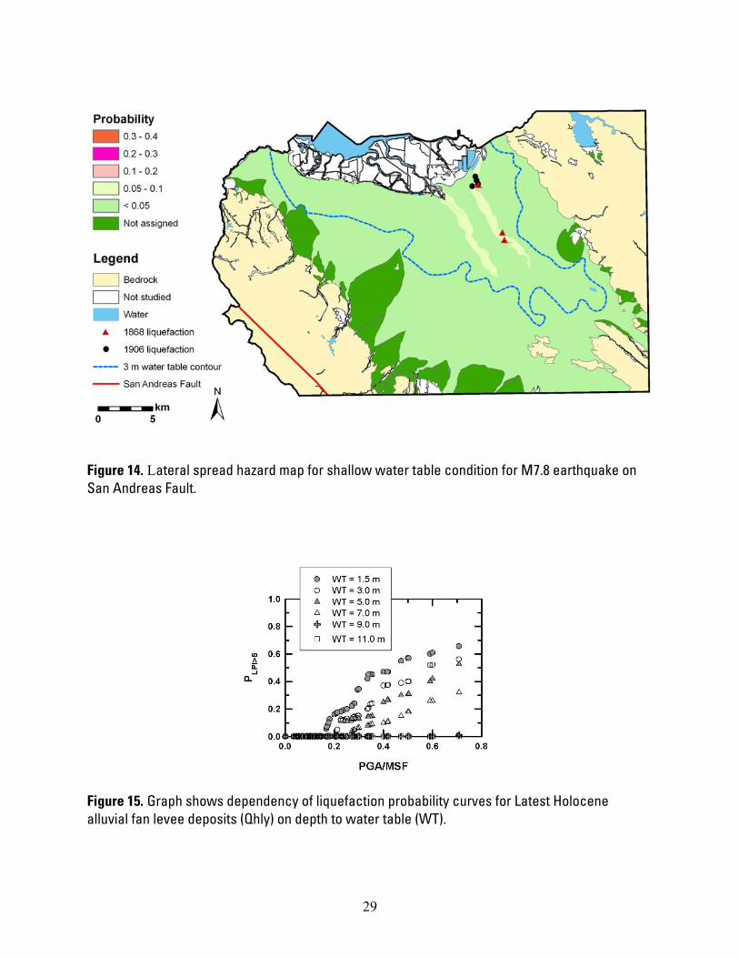
Figure 14. Lateral spread hazard map for shallow water table condition for M7.8 earthquake on San Andreas Fault.

Figure 15. Graph shows dependency of liquefaction probability curves for Latest Holocene alluvial fan levee deposits (Qhly) on depth to water table (WT).

29