A global Constraint for mining Sequential Patterns withGAP constraint

Amina Kemmar1, Samir Loudni2, Yahia Lebbah1

Patrice Boizumault2, and Thierry Charnois3

1LITIO – University of Oran 1 – Algeria, EPSECG of Oran – Algeria2 GREYC (CNRS UMR 6072) – University of Caen – France3LIPN (CNRS UMR 7030) – University PARIS 13 – France

Abstract. Sequential pattern mining (SPM) under gap constraint is a challeng-ing task. Many efficient specialized methods have been developed but they areall suffering from a lack of genericity. The Constraint Programming (CP) ap-proaches are not so effective because of the size of their encodings. In [7], wehave proposed the global constraint PREFIX-PROJECTION for SPM which reme-dies to this drawback. However, this global constraint cannot be directly extendedto support gap constraint. In this paper, we propose the global constraint GAP-SEQ enabling to handle SPM with or without gap constraint. GAP-SEQ relieson the principle of right pattern extensions. Experiments show that our approachclearly outperforms both CP approaches and the state-of-the-art cSpade methodon large datasets.

1 Introduction

Mining sequential patterns (SPM) is an important task in data mining. There are manyuseful applications, including discovering changes in customer behaviors, detecting in-trusion from web logs and finding relevant genes from DNA sequences. In recent yearsmany studies have focused on SPM with gap constraints [16,18]. Limited gaps allow amining process to bear a certain degree of flexibility among correlated pattern elementsin the original sequences. For example, [6] analyses purchase behaviors to reflect prod-ucts usually bought by customers at regular time intervals according to time gaps. Incomputational biology, the gap constraint helps discover periodic patterns with signifi-cant biological and medical values [14].

Mining sequential patterns under gap constraint (GSPM) is a challenging task,since the apriori property does not hold for this problem: a subsequence of a frequentsequence is not necessarily frequent. Several specialized approaches have been pro-posed [6,10,18] but they have a lack of genericity to handle simultaneously varioustypes of constraints. Recently, a few proposals [4,8,11,12] have investigated relation-ships between GSPM and constraint programming (CP) in order to provide a declara-tive approach, while exploiting efficient and generic solving methods. But, due to thesize of the proposed encodings, these CP methods are not as efficient as specializedones. More recently, we have proposed the global constraint PREFIX-PROJECTION forSPM which remedies to this drawback [7]. However, as this global constraint uses theprojected databases principle, it cannot be directly extended to support gap constraint.

arX

iv:1

511.

0835

0v1

[cs

.AI]

26

Nov

201

5

In this paper, we introduce the global constraint GAP-SEQ enabling to handle SPMwith or without gap constraint. GAP-SEQ relies on the principle of right pattern exten-sion and its filtering exploits the prefix anti-monotonicity property of the gap constraintto provide an efficient pruning of the search space. GAP-SEQ enables to handle si-multaneously different types of constraints and its encoding does not require any reifiedconstraints nor any extra variables. Finally, experiments show that our approach clearlyoutperforms CP approaches as well as specialized methods for GSPM and achievesscalability while it is a major issue for CP approaches.

The paper is organized as follows. Section 2 introduces the prefix anti-monotonicityof the gap constraint as well as right pattern extensions that will enable an efficient fil-tering. Section 3 provides a critical review of specialized methods and CP approachesfor sequential pattern mining under gap constraint. Section 4 presents the global con-straint GAP-SEQ. Section 5 reports experiments we performed. Finally, we concludeand draw some perspectives.

2 PreliminariesFirst, we provide the basic definitions for GSPM. Then, we show that the anti-monotonicityproperty of frequency of SPM does not hold for GSPM. Finally, we introduce right pat-tern extensions that will enable an efficient filtering for GSPM.

2.1 Definitions

Let I be a finite set of distinct items. The language of sequences corresponds to LI =In where n ∈ N+.

Definition 1 (sequence, sequence database). A sequence s over LI is an ordered list〈s1s2 . . . sn〉, where si, 1 ≤ i ≤ n, is an item. n is called the length of the sequence s.A sequence database SDB is a set of tuples (sid, s), where sid is a sequence identifierand s a sequence denoted by SDB[sid].

We now define the subsequence relation�[M,N ] under gap[M,N ] constraint whichrestricts the allowed distance between items of subsequences in sequences.

Definition 2 (subsequence relation �[M,N ] under gap[M,N ]). α = 〈α1 . . . αm〉 is asubsequence of s = 〈s1 . . . sn〉, under gap[M,N ], denoted by (α�[M,N ]s), if m ≤ nand, for all 1 ≤ i ≤ m, there exist integers 1 ≤ j1 ≤ . . . ≤ jm ≤ n, such that αi = sji ,and ∀k ∈ {1, ...,m−1},M ≤ jk+1−jk−1 ≤ N . In this context, the pair (s, [j1, jm])denotes an occurrence of α in s, where j1 and jm represent the positions of the firstand last items of α in s. We say that α is contained in s or s is a super-sequence of αunder gap[M,N ]. We also say that α is a gap[M,N ] constrained pattern in s.

– Let AllOcc(α, s) = {[j1, jm] | (s, [j1, jm]) is an occurrence of α in s} be the set ofall the occurrences of some sequence α under gap[M,N ] in s.

– LetAllOcc(α, SDB) = {(sid,AllOcc(α, SDB[sid])) | (sid, SDB[sid]) ∈ SDB}be the set of all the occurrences of some sequence α under gap[M,N ] in SDB.

– Let gap[M,∞] and gap[0, N ] the minimum and the maximum gap constraintsrespectively.

– The relation � stands for �[0,∞] where the gap constraint is inactive.

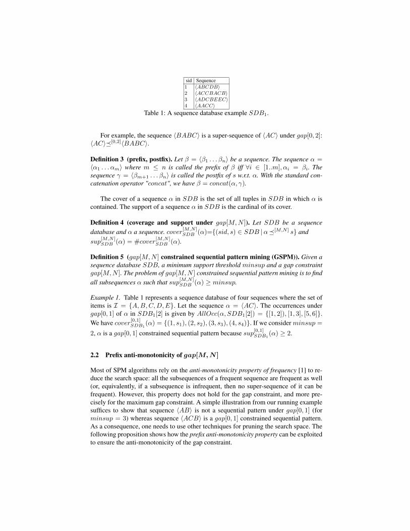
sid Sequence1 〈ABCDB〉2 〈ACCBACB〉3 〈ADCBEEC〉4 〈AACC〉

Table 1: A sequence database example SDB1.

For example, the sequence 〈BABC〉 is a super-sequence of 〈AC〉 under gap[0, 2]:〈AC〉�[0,2]〈BABC〉.

Definition 3 (prefix, postfix). Let β = 〈β1 . . . βn〉 be a sequence. The sequence α =〈α1 . . . αm〉 where m ≤ n is called the prefix of β iff ∀i ∈ [1..m], αi = βi. Thesequence γ = 〈βm+1 . . . βn〉 is called the postfix of s w.r.t. α. With the standard con-catenation operator "concat", we have β = concat(α, γ).

The cover of a sequence α in SDB is the set of all tuples in SDB in which α iscontained. The support of a sequence α in SDB is the cardinal of its cover.

Definition 4 (coverage and support under gap[M,N ]). Let SDB be a sequencedatabase and α a sequence. cover[M,N ]

SDB (α)={(sid, s) ∈ SDB |α�[M,N ] s} andsup

[M,N ]SDB (α) = #cover

[M,N ]SDB (α).

Definition 5 (gap[M,N ] constrained sequential pattern mining (GSPM)). Given asequence database SDB, a minimum support threshold minsup and a gap constraintgap[M,N ]. The problem of gap[M,N ] constrained sequential pattern mining is to findall subsequences α such that sup[M,N ]

SDB (α) ≥ minsup.

Example 1. Table 1 represents a sequence database of four sequences where the set ofitems is I = {A,B,C,D,E}. Let the sequence α = 〈AC〉. The occurrences undergap[0, 1] of α in SDB1[2] is given by AllOcc(α, SDB1[2]) = {[1, 2]), [1, 3], [5, 6]}.We have cover[0,1]SDB1

(α) = {(1, s1), (2, s2), (3, s3), (4, s4)}. If we consider minsup =

2, α is a gap[0, 1] constrained sequential pattern because sup[0,1]SDB1(α) ≥ 2.

2.2 Prefix anti-monotonicity of gap[M,N ]

Most of SPM algorithms rely on the anti-monotonicity property of frequency [1] to re-duce the search space: all the subsequences of a frequent sequence are frequent as well(or, equivalently, if a subsequence is infrequent, then no super-sequence of it can befrequent). However, this property does not hold for the gap constraint, and more pre-cisely for the maximum gap constraint. A simple illustration from our running examplesuffices to show that sequence 〈AB〉 is not a sequential pattern under gap[0, 1] (forminsup = 3) whereas sequence 〈ACB〉 is a gap[0, 1] constrained sequential pattern.As a consequence, one needs to use other techniques for pruning the search space. Thefollowing proposition shows how the prefix anti-monotonicity property can be exploitedto ensure the anti-monotonicity of the gap constraint.

Definition 6 (prefix anti-monotone property). A constraint c is called prefix anti-monotone if for every sequence α satisfying c, every prefix of α also satisfies the con-straint.

Proposition 1. gap[M,N ] is prefix anti-monotone.

Proof. Let α = 〈α1 . . . αm〉 and s = 〈s1 . . . sn〉 be two sequences s.t. α�[M,N ]s andm ≤ n. By definition, there exist integers 1 ≤ j1 ≤ . . . ≤ jm ≤ n, such that αi = sji ,and ∀k ∈ {1, ...,m − 1},M ≤ jk+1 − jk − 1 ≤ N . As a consequence, the propertyalso holds for every prefix of α. 2

Hence, if a sequence α does not satisfy gap[M,N ], then all sequences that haveα as prefix will not satisfy this constraint. Sect. 4.2 shows how this property can beexploited to provide an efficient filtering.

2.3 Right pattern extensions

Right pattern extensions of some pattern p gives all the possible subsequences whichcan be appended at right of p to form a gap[M,N ] constrained pattern. According toproposition 1, the set of all items locally frequent within the right pattern extensions ofp in SDB can be used to extend p. In the following, we introduce an operator allowingto compute all the right pattern extensions of a pattern w.r.t. gap[M,N ].

Definition 7 (Right pattern extensions). Given some sequence (sid, s) and a patternp s.t. p�[M,N ]s. The right pattern extensions of p in s, denoted by Ext[M,N ]

R (p, s),is the collection of legal subsequences of s located at the right of p and satisfyinggap[M,N ]. To define Ext[M,N ]

R (p, s), we need to define BE[M,N ](p, s) basic rightextensions :

BE[M,N ](p, s) =⋃

[j1,jm]∈AllOcc(p,s)

{(jm, SubSeq(s, jm +M + 1,min(jm +N + 1,#s)))}

where SubSeq(s, i1, i2) ={〈s[i1], ..., s[i2]〉 if i1 ≤ i2 ≤ #s〈〉 otherwise

Right pattern extensions Ext[M,N ]R (p, s) is defined as follows:

Ext[M,N ]R (p, s) =

{Sb | (j′m, Sb) ∈ BE[M,N ](p, s)∧ if N ≥ #s

j′m = min(jm,Sb)∈BE[M,N](p,s){jm}}⋃(jm,Sb)∈BE[M,N](p,s){Sb} otherwise

(1)

Formula (1) states exactly the set of all possible extensions of pattern p within s. Incase where (N ≥ #s), since that any extension fromBE[M,N ](p, s) always reaches theend of the sequence s, thus all possible extensions can be aggregated within one uniqueextension going from the lowest starting position j′m = min(jm,Sb)∈BE[M,N](p,s){jm}.We point out that these cases (N ≥ #s) cover the special case of no gap gap[0,∞].

The right pattern extensions of p in SDB is the collection of all its right patternextensions in all sequences of SDB:

Ext[M,N ]R (p, SDB) =

⋃(sid,s)∈SDB

{(sid, Ext[M,N ]R (p, s))} (2)

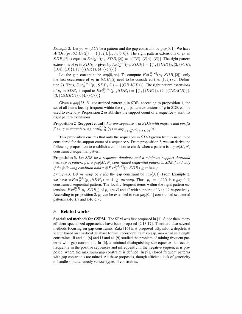
Example 2. Let p1 = 〈AC〉 be a pattern and the gap constraint be gap[0, 1]. We haveAllOcc(p1, SDB1[2]) = {[1, 2]), [1, 3], [5, 6]}. The right pattern extensions of p1 inSDB1[2] is equal to Ext[0,1]R (p1, SDB1[2]) = {〈CB〉, 〈BA〉, 〈B〉}. The right patternextensions of p1 in SDB1 is given byExt[0,1]R (p1, SDB1) = {(1, {〈DB〉}), (2, {〈CB〉,〈BA〉, 〈B〉}), (3, {〈BE〉}), (4, {〈C〉})}.

Let the gap constraint be gap[0,∞]. To compute Ext[0,∞]R (p1, SDB1[2]), only

the first occurrence of p1 in SDB1[2] need to be considered (i.e. [1, 2]) (cf. Defini-tion 7). Thus, Ext[0,∞]

R (p1, SDB1[2]) = {〈CBACB〉}). The right pattern extensionsof p1 in SDB1 is equal to Ext[0,∞]

R (p1, SDB1) = {(1, {〈DB〉}), (2, {〈CBACB〉}),(3, {〈BEEC〉}), (4, {〈C〉})}.

Given a gap[M,N ] constrained pattern p in SDB, according to proposition 1, theset of all items locally frequent within the right pattern extensions of p in SDB can beused to extend p. Proposition 2 establishes the support count of a sequence γ w.r.t. itsright pattern extensions.

Proposition 2 (Support count). For any sequence γ in SDB with prefix α and postfixβ s.t. γ = concat(α, β), sup[M,N ]

SDB (γ) = supExt

[M,N]R (α,SDB)

(β).

This proposition ensures that only the sequences in SDB grown from α need to beconsidered for the support count of a sequence γ. From proposition 2, we can derive thefollowing proposition to establish a condition to check when a pattern is a gap[M,N ]constrained sequential pattern.

Proposition 3. Let SDB be a sequence database and a minimum support thresholdminsup. A pattern p is a gap[M,N ] constrained sequential pattern in SDB if and onlyif the following condition holds: #Ext[M,N ]

R (p, SDB) ≥ minsupExample 3. Let minsup be 2 and the gap constraint be gap[0, 1]. From Example 2,we have #Ext

[0,1]R (p1, SDB1) = 4 ≥ minsup. Thus, p1 = 〈AC〉 is a gap[0, 1]

constrained sequential pattern. The locally frequent items within the right pattern ex-tensions Ext[0,1]R (p1, SDB1) of p1 are B and C with supports of 3 and 2 respectively.According to proposition 2, p1 can be extended to two gap[0, 1] constrained sequentialpatterns 〈ACB〉 and 〈ACC〉 .

3 Related worksSpecialized methods for GSPM. The SPM was first proposed in [1]. Since then, manyefficient specialized approaches have been proposed [2,13,17]. There are also severalmethods focusing on gap constraints. Zaki [16] first proposed cSpade, a depth-firstsearch based on a vertical database format, incorporating max-gap, max-span and lengthconstraints. Ji and al. [6] and Li and al. [9] studied the problem of mining frequent pat-terns with gap constraints. In [6], a minimal distinguishing subsequence that occursfrequently in the positive sequences and infrequently in the negative sequences is pro-posed, where the maximum gap constraint is defined. In [9], closed frequent patternswith gap constraints are mined. All these proposals, though efficient, lack of genericityto handle simultaneously various types of constraints.

CP Methods for GSPM. There are few methods for SPM with gap constraints usingCP. [11] have proposed to model a sequence using an automaton capturing all sub-sequences that can occur in it. The gap constraint is encoded by removing from theautomaton all transitions that does not respect the gap constraint. [8] have proposeda CSP model for SPM with explicit wildcards1. The gap constraints is enforced us-ing the regular global constraint. [12] have proposed two CP encodings for the SPM.The first one uses a global constraint to encode the subsequence relation (denotedglobal-p.f), while the second one (denoted decomposed-p.f) encodes explic-itly this relation using additional variables and constraints in order to support constraintslike gap. However, all these proposals usually lead to constraints network of huge size.Space complexity is clearly identified as the main bottleneck behind the competitive-ness of these declarative approaches. In [7], we have proposed the global constraintPREFIX-PROJECTION for sequential pattern mining which remedies to this drawback.However, this constraint cannot be directly extended to handle gap constraints. Thisrequires changing the way the subsequence relation is encoded.

The next section introduces the global constraint GAP-SEQ enabling to handleSPM with or without gap constraints. GAP-SEQ relies on the prefix anti-monotonicityof the gap constraint and on the right pattern extensions to provide an efficient filtering.This global constraint does not require any reified constraints nor any extra variables toencode the subsequence relation.

4 GAP-SEQ global constraintThis section is devoted to the GAP-SEQ global constraint. Section 4.1 defines theGAP-SEQ global constraint and presents the CSP modeling. Section 4.2 shows how thefiltering can take advantage of the prefix anti-monotonicity property of the gap[M,N ]constraint (see Proposition 6) and of the right pattern extensions (see Proposition 5) toremove inconsistent values from the domain of a future variable. Section 4.3 details thefiltering algorithm and Section 4.4 provides its temporal and spatial complexities.

4.1 CSP modeling for GSPM

A Constraint Satisfaction Problem (CSP) consists of a setX of n variables, a domainDmapping each variable Xi ∈ X to a finite set of values D(Xi), and a set of constraintsC. An assignment σ is a mapping from variables in X to values in their domains. Aconstraint c ∈ C is a subset of the cartesian product of the domains of the variables thatoccur in c. The goal is to find an assignment such that all constraints are satisfied.(a) Variables and domains. Let P be the unknown pattern of size ` we are lookingfor. The symbol 2 stands for an empty item and denotes the end of a sequence. Weencode the unknown pattern P of maximum length ` with a sequence of ` variables〈P1, P2, . . . , P`〉. Each variable Pj represents the item in the jth position of the se-quence. The size ` of P is determined by the length of the longest sequence of SDB.The domains of variables are defined as follows: (i) D(P1) = I to avoid the emptysequence, and (ii) ∀i ∈ [2 . . . `], D(Pi) = I ∪ {2}. To allow patterns with less than `items, we impose that ∀i ∈ [2..(`−1)], (Pi = 2)→ (Pi+1 = 2).

1 A wildcard is a special symbol that matches any item of I including itself.

(b) Definition of GAP-SEQ. The global constraint GAP-SEQ encodes both subse-quence relation �[M,N ] under gap constraint gap[M,N ] and minimum frequency con-straint directly on the data.

Definition 8 (GAP-SEQ global constraint). Let P = 〈P1, P2, . . . , P`〉 be a patternof size ` and gap[M,N ] be the gap constraint. 〈d1, ..., d`〉 ∈ D(P1)× . . .×D(P`) is asolution of GAP-SEQ(P, SDB,minsup,M,N) iff sup[M,N ]

SDB (〈d1, ..., d`〉) ≥ minsup.

Proposition 4. GAP-SEQ(P, SDB,minsup,M,N) has a solution iff there exists anassignment σ = 〈d1, ..., d`〉 of variables of P s.t. #Ext[M,N ]

R (σ, SDB) ≥ minsup.

Proof: This is a direct consequence of proposition 3. 2(c) Other SPM constraints can be directly modeled as follows:- Minimum Size constraint restricts the number of items of a pattern to be at least `min:minSize(P, `min) ≡

∧i=`min

i=1 (Pi 6= �)- Maximum Size constraint restricts the number of items of a pattern to be at most `max:maxSize(P, `max) ≡

∧i=`i=`max+1(Pi = �)

- Membership constraint states that a subset of items V must belong (or not) to theextracted patterns. item(P, V ) ≡

∧t∈V Among(P, {t}, l, u) enforces that items of V

should occur at least l times and at most u times in P . To forbid items of V to occur inP , l and u must be set to 0.

4.2 Principles of filtering

(a) Maintaining a local consistency. SPM is a challenging task due to the exponen-tial number of candidates that should be parsed to find the frequent patterns. For in-stance, with k items there are O(nk) potentially candidate patterns of length at most kin a sequence of size n. With gap constraints, the problem is even much harder sincethe complexity of checking for subsequences taking a gap constraint into account ishigher than the complexity of the standard subsequence relation. Furthermore, the NP-hardness of mining maximal2 frequent sequences was established in [15] by provingthe #P-completeness of the problem of counting the number of maximal frequent se-quences. Hence, ensuring Domain Consistency (DC) for GAP-SEQ i.e., finding, forevery variable Pj , a value dj ∈ D(Pj), satisfying the constraint is NP-hard.

So, the filtering of GAP-SEQ constraint maintains a consistency lower than DC.This consistency is based on specific properties of the gap[M,N ] constraint and resem-bles forward-checking (regarding Proposition 5). GAP-SEQ is considered as a globalconstraint, since all variables share the same internal data structures that awake anddrive the filtering. The prefix anti-monotonicity property of the gap[M,N ] constraint(see Proposition 6) and of the right pattern extensions (see Proposition 5) will enable toremove inconsistent values from the domain of a future variable.(b) Detecting inconsistent values. Let RF [M,N ](σ, SDB) be the set of locally fre-quent items within the right pattern extensions, defined by {v ∈ I |#{sid | (sid, E) ∈Ext

[M,N ]R (σ, SDB) ∧ (∃α ∈ E ∧ 〈v〉�α)} ≥ minsup}. The following proposition

2 A sequential pattern p is maximal if there is no sequential pattern q such that p�q.

characterizes values, of a future (unassigned) variable Pj+1, that are consistent with thecurrent assignment of variables 〈P1, . . . , Pj〉.

Proposition 5. Let 3 σ= 〈d1, . . . , dj〉 be a current assignment of variables 〈P1, . . . , Pj〉,Pj+1 be a future variable. A value d ∈ D(Pj+1) occurs in a solution for the global con-straint GAP-SEQ(P, SDB,minsup,M,N) iff d ∈ RF [M,N ](σ, SDB).

Proof: Assume that σ = 〈d1, . . . , dj〉 is gap[M,N ] constrained sequential patternin SDB. Suppose that value d ∈ D(Pj+1) appears in RF [M,N ](σ, SDB). As thelocal support of d within the right extensions is equal to sup

Ext[M,N]R (σ,SDB)

(〈d〉),

from proposition 2 we have sup[M,N ]SDB (concat(σ, 〈d〉)) = sup

Ext[M,N]R (σ,SDB)

(〈d〉).Hence, we can get a new assignment σ ∪ 〈d〉 that satisfies the constraint. Therefore,d ∈ D(Pj+1) participates in a solution. 2

From proposition 5 and according to the prefix anti-monotonicity property of thegap constraint, we can derive the following pruning rule:

Proposition 6. Let σ = 〈d1, . . . , dj〉 be a current assignment of variables 〈P1, . . . ,

Pj〉. All values d ∈ D(Pj+1) that are not in RF [M,N ](σ, SDB) can be removed fromthe domain of variable Pj+1.

Example 4. Consider the running example of Table 1, let minsup be 2 and the gapconstraint be gap[1, 2]. Let P = 〈P1, P2, P3, P4〉 with D(P1) = I and D(P2) =

D(P3) = D(P4) = I ∪{2}. Suppose that σ(P1) = A. We have Ext[1,2]R (〈A〉, SDB1)= {(1, {〈CD〉}), (2, {〈CB〉, 〈B〉}), (3, {〈CB〉}), (4, {〈CC〉, 〈C〉})}. As B and C arethe only locally frequent items inExt[1,2]R (〈A〉, SDB1), GAP-SEQ will remove valuesA, D and E from D(P2).

The filtering of GAP-SEQ relies on Proposition 6 and is detailed in the next section.

4.3 Filtering algorithm

Algorithm 1 describes the pseudo-code of GAP-SEQ filtering algorithm. It takes asinput: the index j of the last assigned variable in P , the current partial assignmentσ = 〈σ(P1), . . . , σ(Pj)〉, the minimum support threshold minsup, the minimum andthe maximum gaps. The internal data-structureALLOCC stores all the intermediate oc-currences of patterns in SDB, whereALLOCCj = AllOcc(σ, SDB), for j ∈ [1 . . . `].If σ = 〈〉, then ALLOCC0 = {(sid, [1,#s]) | (sid, s) ∈ SDB}. ALLOCCj is com-puted incrementally from ALLOCCj−1 in order to enhance the efficiency.

Algorithm 1 starts by computing the right pattern extensions ExtR of σ in SDB(line 1) by calling function GETRIGHTEXT (see Algorithm 2). Then, it checks whetherthe current assignment σ satisfies the constraint (see Proposition 4) (line 2). If not,we stop growing σ and return False. Otherwise, the algorithm checks if the last as-signed variable Pj is instantiated to 2 (line 4). If so, the end of the sequence is reached(since value 2 can only appear at the end) and the sequence 〈σ(P1), . . . , σ(Pj)〉 is a

3 We indifferently denote σ by 〈d1, . . . , dj〉 or by 〈σ(P1), . . . , σ(Pj)〉.

Algorithm 1: FILTER-GAP-SEQ(SDB, σ, j, P , minsup, M , N )Data: SDB: initial database; σ: current assignment 〈σ(P1), . . . , σ(Pj)〉;minsup: the minimum support

threshold;ALLOCC: internal data structure for storing occurrences of patterns in SDB;ExtR: internaldata structure for storing right pattern extensions of σ in SDB.

begin1 ExtR ← GETRIGHTEXT(SDB,ALLOCCj−1, σ,M,N) ;2 if (#ExtR < minsup) then3 return False ;

4 if (j ≥ 2 ∧ σ(Pj) = 2) then5 for k ← j + 1 to ` do6 Pk ← 2 ;

else7 RF ← GETFREQITEMS(SDB,ExtR,minsup) ;8 foreach a ∈ D(Pj+1) s.t.(a 6= 2 ∧ a /∈ RF) do9 D(Pj+1)← D(Pj+1)− {a} ;

10 return True ;

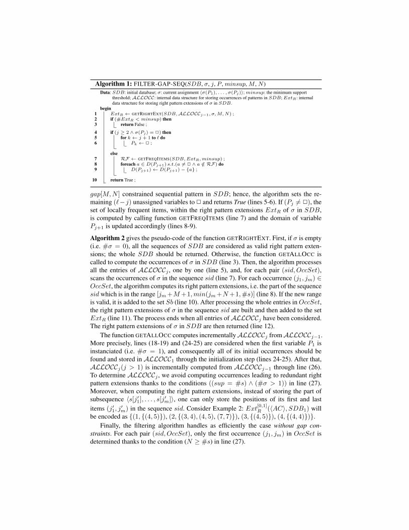
gap[M,N ] constrained sequential pattern in SDB; hence, the algorithm sets the re-maining (`− j) unassigned variables to 2 and returns True (lines 5-6). If (Pj 6= 2), theset of locally frequent items, within the right pattern extensions ExtR of σ in SDB,is computed by calling function GETFREQITEMS (line 7) and the domain of variablePj+1 is updated accordingly (lines 8-9).

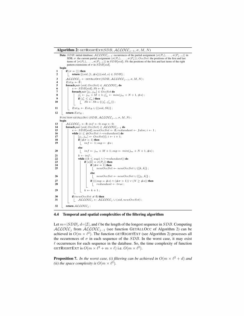
Algorithm 2 gives the pseudo-code of the function GETRIGHTEXT. First, if σ is empty(i.e. #σ = 0), all the sequences of SDB are considered as valid right pattern exten-sions; the whole SDB should be returned. Otherwise, the function GETALLOCC iscalled to compute the occurrences of σ in SDB (line 3). Then, the algorithm processesall the entries of ALLOCCj , one by one (line 5), and, for each pair (sid,OccSet),scans the occurrences of σ in the sequence sid (line 7). For each occurrence (j1, jm) ∈OccSet, the algorithm computes its right pattern extensions, i.e. the part of the sequencesid which is in the range [jm+M+1,min(jm+N+1,#s)] (line 8). If the new rangeis valid, it is added to the set Sb (line 10). After processing the whole entries inOccSet,the right pattern extensions of σ in the sequence sid are built and then added to the setExtR (line 11). The process ends when all entries ofALLOCCj have been considered.The right pattern extensions of σ in SDB are then returned (line 12).

The function GETALLOCC computes incrementallyALLOCCj fromALLOCCj−1.More precisely, lines (18-19) and (24-25) are considered when the first variable P1 isinstanciated (i.e. #σ = 1), and consequently all of its initial occurrences should befound and stored in ALLOCC1 through the initialization step (lines 24-25). After that,ALLOCCj(j > 1) is incrementally computed from ALLOCCj−1 through line (26).To determine ALLOCCj , we avoid computing occurrences leading to redundant rightpattern extensions thanks to the conditions ((sup = #s) ∧ (#σ > 1)) in line (27).Moreover, when computing the right pattern extensions, instead of storing the part ofsubsequence 〈s[j′1], . . . , s[j′m]〉, one can only store the positions of its first and lastitems (j′1, j

′m) in the sequence sid. Consider Example 2: Ext[0,1]R (〈AC〉, SDB1) will

be encoded as {(1, {(4, 5)}), (2, {(3, 4), (4, 5), (7, 7)}), (3, {(4, 5)}), (4, {(4, 4)})}.Finally, the filtering algorithm handles as efficiently the case without gap con-

straints. For each pair (sid,OccSet), only the first occurrence (j1, jm) in OccSet isdetermined thanks to the condition (N ≥ #s) in line (27).

Algorithm 2: GETRIGHTEXT(SDB, ALLOCCj−1, σ, M , N )Data: SDB: initial database;ALLOCCj−1: occurrences of the partial assignment 〈σ(P1), . . . , σ(Pj−1)〉 in

SDB; σ: the current partial assignment 〈σ(P1), . . . , σ(Pj)〉;OccSet: the positions of the first and lastitems of 〈σ(P1), . . . , σ(Pj−1)〉 in SDB[sid]; Sb: the positions of the first and last items of the rightpattern extensions of σ in SDB[sid].

begin1 if (σ = 〈〉) then2 return {(sid, [1,#s])|(sid, s) ∈ SDB} ;

3 ALLOCCj ← GETALLOCC(SDB,ALLOCCj−1, σ,M,N) ;4 ExtR ← ∅ ;5 foreach pair (sid,OccSet) ∈ ALLOCCj do6 s← SDB[sid]; Sb← ∅ ;7 foreach pair [j1, jm] ∈ OccSet do8 j′1 ← jm +M + 1; j′m ← min(jm +N + 1,#s) ;9 if (j′1 ≤ j

′m) then

10 Sb← Sb ∪ {(j′1, j′m)} ;

11 ExtR ← ExtR ∪ {(sid, Sb)} ;

12 returnExtR ;

FUNCTION GETALLOCC (SDB,ALLOCCj−1, σ,M ,N ) ;begin

13 ALLOCCj ← ∅; inf ← 0; sup← 0;14 foreach pair (sid,OccSet) ∈ ALLOCCj−1 do15 s← SDB[sid]; newOccSet← ∅; redundant← false; i← 1 ;16 while (i ≤ #OccSet ∧¬redundant) do17 [j1, jm]← OccSet[i]; i← i+ 1;18 if (#σ = 1) then19 inf ← 1; sup← #s ;

else20 inf ← jm +M + 1; sup← min(jm +N + 1,#s) ;

21 k ← inf ;22 while ((k ≤ sup) ∧ (¬redundant)) do23 if (s[k] = σ(Pj)) then24 if (#σ = 1) then25 newOccSet← newOccSet ∪ {[k, k]} ;

else26 newOccSet← newOccSet ∪ {[j1, k]} ;

27 if (((sup = #s) ∧ (#σ > 1)) ∨ (N ≥ #s)) then28 redundant← true ;

29 k ← k + 1 ;

30 if (newOccSet 6= ∅) then31 ALLOCCj ← ALLOCCj ∪ (sid, newOccSet) ;

32 returnALLOCCj ;

4.4 Temporal and spatial complexities of the filtering algorithm

Letm=|SDB|, d=|I|, and ` be the length of the longest sequence in SDB. ComputingALLOCCj from ALLOCCj−1 (see function GETALLOCC of Algorithm 2) can beachieved in O(m × `2). The function GETRIGHTEXT (see Algorithm 2) processes allthe occurrences of σ in each sequence of the SDB. In the worst case, it may exist` occurrences for each sequence in the database. So, the time complexity of functionGETRIGHTEXT is O(m× `2 +m× `) i.e. O(m× `2).

Proposition 7. In the worst case, (i) filtering can be achieved in O(m × `2 + d) and(ii) the space complexity is O(m× `2).

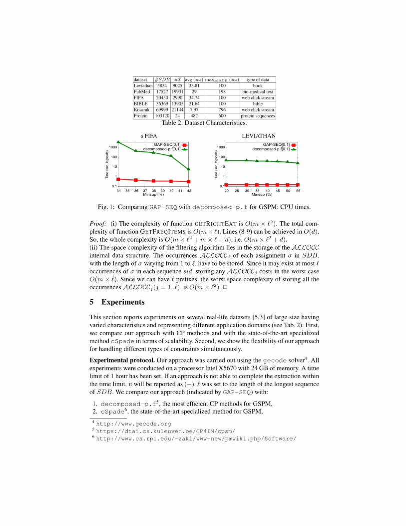
dataset #SDB #I avg (#s) maxs∈SDB (#s) type of dataLeviathan 5834 9025 33.81 100 bookPubMed 17527 19931 29 198 bio-medical textFIFA 20450 2990 34.74 100 web click streamBIBLE 36369 13905 21.64 100 bibleKosarak 69999 21144 7.97 796 web click streamProtein 103120 24 482 600 protein sequences

Table 2: Dataset Characteristics.

s FIFA LEVIATHAN

0.1

1

10

100

1000

34 35 36 37 38 39 40 41 42

Tim

e (

sec,

logsc

ale

)

Minsup (%)

GAP-SEQ[0,1]decomposed-p.f[0,1]

0.1

1

10

100

1000

20 25 30 35 40 45 50 55

Tim

e (

sec,

logsc

ale

)

Minsup (%)

GAP-SEQ[0,1]decomposed-p.f[0,1]

Fig. 1: Comparing GAP-SEQ with decomposed-p.f for GSPM: CPU times.

Proof: (i) The complexity of function GETRIGHTEXT is O(m × `2). The total com-plexity of function GETFREQITEMS is O(m× `). Lines (8-9) can be achieved in O(d).So, the whole complexity is O(m× `2 +m× `+ d), i.e. O(m× `2 + d).(ii) The space complexity of the filtering algorithm lies in the storage of the ALLOCCinternal data structure. The occurrences ALLOCCj of each assignment σ in SDB,with the length of σ varying from 1 to `, have to be stored. Since it may exist at most `occurrences of σ in each sequence sid, storing any ALLOCCj costs in the worst caseO(m × `). Since we can have ` prefixes, the worst space complexity of storing all theoccurrences ALLOCCj(j = 1..`), is O(m× `2). 2

5 Experiments

This section reports experiments on several real-life datasets [5,3] of large size havingvaried characteristics and representing different application domains (see Tab. 2). First,we compare our approach with CP methods and with the state-of-the-art specializedmethod cSpade in terms of scalability. Second, we show the flexibility of our approachfor handling different types of constraints simultaneously.

Experimental protocol. Our approach was carried out using the gecode solver4. Allexperiments were conducted on a processor Intel X5670 with 24 GB of memory. A timelimit of 1 hour has been set. If an approach is not able to complete the extraction withinthe time limit, it will be reported as (−). ` was set to the length of the longest sequenceof SDB. We compare our approach (indicated by GAP-SEQ) with:

1. decomposed-p.f5, the most efficient CP methods for GSPM,2. cSpade6, the state-of-the-art specialized method for GSPM,4 http://www.gecode.org5 https://dtai.cs.kuleuven.be/CP4IM/cpsm/6 http://www.cs.rpi.edu/~zaki/www-new/pmwiki.php/Software/

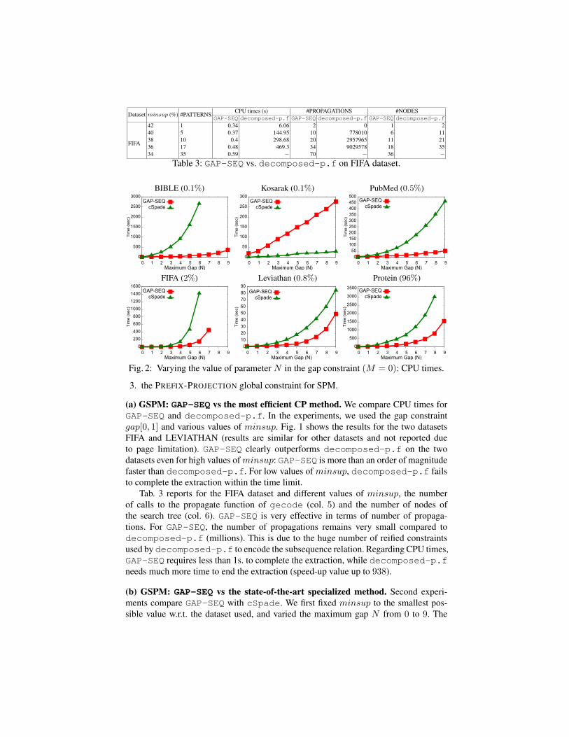
Dataset minsup (%) #PATTERNSCPU times (s) #PROPAGATIONS #NODES

GAP-SEQ decomposed-p.f GAP-SEQ decomposed-p.f GAP-SEQ decomposed-p.f

FIFA

42 1 0.34 6.06 2 0 1 240 5 0.37 144.95 10 778010 6 1138 10 0.4 298.68 20 2957965 11 2136 17 0.48 469.3 34 9029578 18 3534 35 0.59 − 70 − 36 −

Table 3: GAP-SEQ vs. decomposed-p.f on FIFA dataset.

BIBLE (0.1%) Kosarak (0.1%) PubMed (0.5%)

0

500

1000

1500

2000

2500

3000

0 1 2 3 4 5 6 7 8 9

Tim

e (

se

c)

Maximum Gap (N)

GAP-SEQcSpade

0

50

100

150

200

250

300

0 1 2 3 4 5 6 7 8 9

Tim

e (

se

c)

Maximum Gap (N)

GAP-SEQcSpade

0

50

100

150

200

250

300

350

400

450

500

0 1 2 3 4 5 6 7 8 9

Tim

e (

se

c)

Maximum Gap (N)

GAP-SEQcSpade

FIFA (2%) Leviathan (0.8%) Protein (96%)

0

200

400

600

800

1000

1200

1400

1600

0 1 2 3 4 5 6 7 8 9

Tim

e (

se

c)

Maximum Gap (N)

GAP-SEQcSpade

0

10

20

30

40

50

60

70

80

90

0 1 2 3 4 5 6 7 8 9

Tim

e (

se

c)

Maximum Gap (N)

GAP-SEQcSpade

0

500

1000

1500

2000

2500

3000

3500

0 1 2 3 4 5 6 7 8 9

Tim

e (

se

c)

Maximum Gap (N)

GAP-SEQcSpade

Fig. 2: Varying the value of parameter N in the gap constraint (M = 0): CPU times.

3. the PREFIX-PROJECTION global constraint for SPM.

(a) GSPM: GAP-SEQ vs the most efficient CP method. We compare CPU times forGAP-SEQ and decomposed-p.f. In the experiments, we used the gap constraintgap[0, 1] and various values of minsup. Fig. 1 shows the results for the two datasetsFIFA and LEVIATHAN (results are similar for other datasets and not reported dueto page limitation). GAP-SEQ clearly outperforms decomposed-p.f on the twodatasets even for high values ofminsup: GAP-SEQ is more than an order of magnitudefaster than decomposed-p.f. For low values of minsup, decomposed-p.f failsto complete the extraction within the time limit.

Tab. 3 reports for the FIFA dataset and different values of minsup, the numberof calls to the propagate function of gecode (col. 5) and the number of nodes ofthe search tree (col. 6). GAP-SEQ is very effective in terms of number of propaga-tions. For GAP-SEQ, the number of propagations remains very small compared todecomposed-p.f (millions). This is due to the huge number of reified constraintsused by decomposed-p.f to encode the subsequence relation. Regarding CPU times,GAP-SEQ requires less than 1s. to complete the extraction, while decomposed-p.fneeds much more time to end the extraction (speed-up value up to 938).

(b) GSPM: GAP-SEQ vs the state-of-the-art specialized method. Second experi-ments compare GAP-SEQ with cSpade. We first fixed minsup to the smallest pos-sible value w.r.t. the dataset used, and varied the maximum gap N from 0 to 9. The

BIBLE Kosarak PubMed

0

50

100

150

200

250

300

350

0.5 0.6 0.7 0.8 0.9 1

Tim

e (

se

c)

Minsup (%)

GAP-SEQcSpade

0

100

200

300

400

500

600

700

0.06 0.1 0.15 0.2 0.25 0.3

Tim

e (

se

c)

Minsup (%)

GAP-SEQcSpade

0

500

1000

1500

2000

2500

3000

3500

4000

0.1 0.2 0.3 0.4 0.5 0.6 0.7 0.8 0.9 1

Tim

e (

se

c)

Minsup (%)

GAP-SEQcSpade

FIFA Leviathan Protein

0

500

1000

1500

2000

2500

3000

3 4 5 6 7 8 9 10

Tim

e (

se

c)

Minsup (%)

GAP-SEQcSpade

0

50

100

150

200

250

0.5 1 1.5 2 2.5 3 3.5 4 4.5 5

Tim

e (

se

c)

Minsup (%)

GAP-SEQcSpade

0

500

1000

1500

2000

2500

3000

3500

96 97 98 99 99.99

Tim

e (

se

c)

Minsup (%)

GAP-SEQcSpade

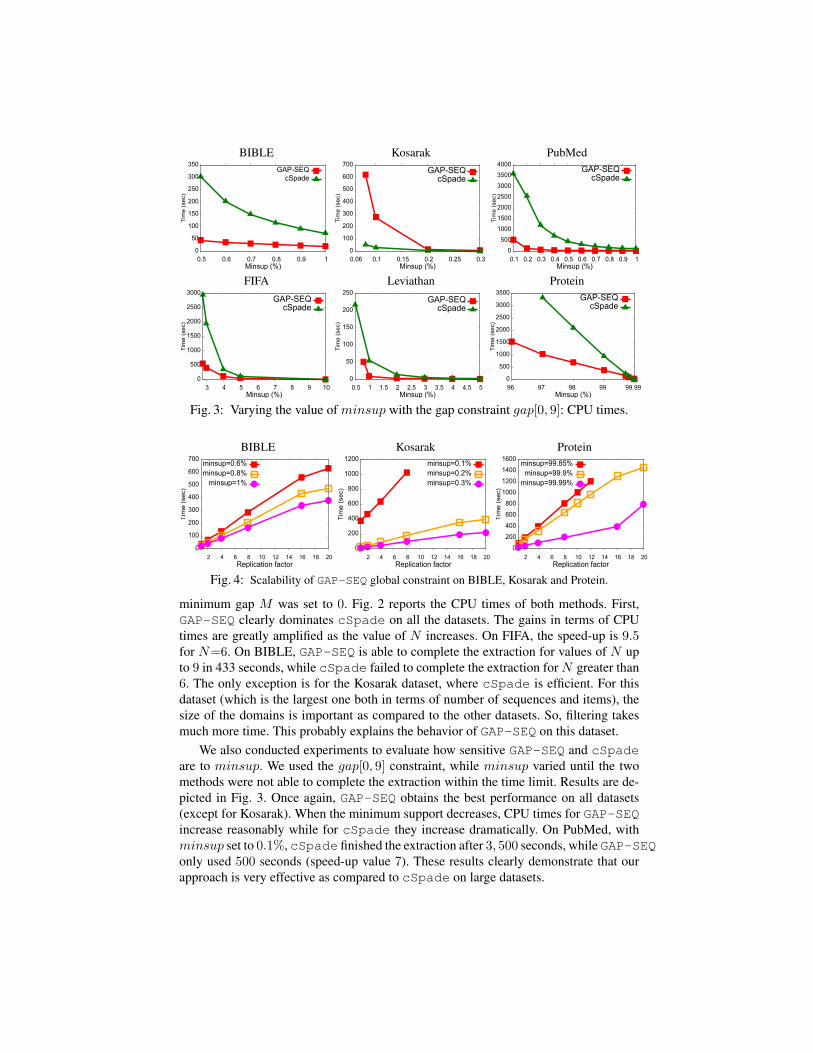
Fig. 3: Varying the value of minsup with the gap constraint gap[0, 9]: CPU times.

BIBLE Kosarak Protein

0

100

200

300

400

500

600

700

2 4 6 8 10 12 14 16 18 20

Tim

e (

se

c)

Replication factor

minsup=0.6%

minsup=0.8%

minsup=1%

0

200

400

600

800

1000

1200

2 4 6 8 10 12 14 16 18 20

Tim

e (

se

c)

Replication factor

minsup=0.1%

minsup=0.2%

minsup=0.3%

0

200

400

600

800

1000

1200

1400

1600

2 4 6 8 10 12 14 16 18 20

Tim

e (

se

c)

Replication factor

minsup=99.85%

minsup=99.9%

minsup=99.99%

Fig. 4: Scalability of GAP-SEQ global constraint on BIBLE, Kosarak and Protein.

minimum gap M was set to 0. Fig. 2 reports the CPU times of both methods. First,GAP-SEQ clearly dominates cSpade on all the datasets. The gains in terms of CPUtimes are greatly amplified as the value of N increases. On FIFA, the speed-up is 9.5for N=6. On BIBLE, GAP-SEQ is able to complete the extraction for values of N upto 9 in 433 seconds, while cSpade failed to complete the extraction for N greater than6. The only exception is for the Kosarak dataset, where cSpade is efficient. For thisdataset (which is the largest one both in terms of number of sequences and items), thesize of the domains is important as compared to the other datasets. So, filtering takesmuch more time. This probably explains the behavior of GAP-SEQ on this dataset.

We also conducted experiments to evaluate how sensitive GAP-SEQ and cSpadeare to minsup. We used the gap[0, 9] constraint, while minsup varied until the twomethods were not able to complete the extraction within the time limit. Results are de-picted in Fig. 3. Once again, GAP-SEQ obtains the best performance on all datasets(except for Kosarak). When the minimum support decreases, CPU times for GAP-SEQincrease reasonably while for cSpade they increase dramatically. On PubMed, withminsup set to 0.1%, cSpade finished the extraction after 3, 500 seconds, while GAP-SEQonly used 500 seconds (speed-up value 7). These results clearly demonstrate that ourapproach is very effective as compared to cSpade on large datasets.

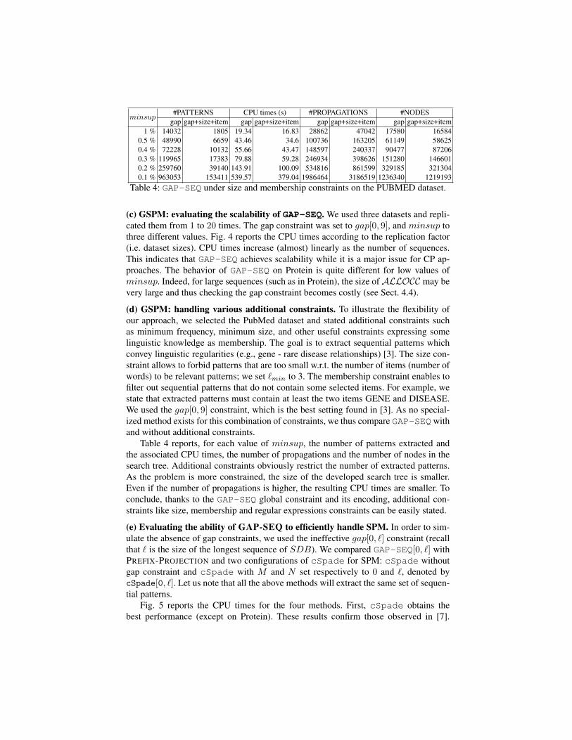
minsup#PATTERNS CPU times (s) #PROPAGATIONS #NODES

gap gap+size+item gap gap+size+item gap gap+size+item gap gap+size+item1 % 14032 1805 19.34 16.83 28862 47042 17580 16584

0.5 % 48990 6659 43.46 34.6 100736 163205 61149 586250.4 % 72228 10132 55.66 43.47 148597 240337 90477 872060.3 % 119965 17383 79.88 59.28 246934 398626 151280 1466010.2 % 259760 39140 143.91 100.09 534816 861599 329185 3213040.1 % 963053 153411 539.57 379.04 1986464 3186519 1236340 1219193

Table 4: GAP-SEQ under size and membership constraints on the PUBMED dataset.

(c) GSPM: evaluating the scalability of GAP-SEQ. We used three datasets and repli-cated them from 1 to 20 times. The gap constraint was set to gap[0, 9], and minsup tothree different values. Fig. 4 reports the CPU times according to the replication factor(i.e. dataset sizes). CPU times increase (almost) linearly as the number of sequences.This indicates that GAP-SEQ achieves scalability while it is a major issue for CP ap-proaches. The behavior of GAP-SEQ on Protein is quite different for low values ofminsup. Indeed, for large sequences (such as in Protein), the size ofALLOCC may bevery large and thus checking the gap constraint becomes costly (see Sect. 4.4).

(d) GSPM: handling various additional constraints. To illustrate the flexibility ofour approach, we selected the PubMed dataset and stated additional constraints suchas minimum frequency, minimum size, and other useful constraints expressing somelinguistic knowledge as membership. The goal is to extract sequential patterns whichconvey linguistic regularities (e.g., gene - rare disease relationships) [3]. The size con-straint allows to forbid patterns that are too small w.r.t. the number of items (number ofwords) to be relevant patterns; we set `min to 3. The membership constraint enables tofilter out sequential patterns that do not contain some selected items. For example, westate that extracted patterns must contain at least the two items GENE and DISEASE.We used the gap[0, 9] constraint, which is the best setting found in [3]. As no special-ized method exists for this combination of constraints, we thus compare GAP-SEQwithand without additional constraints.

Table 4 reports, for each value of minsup, the number of patterns extracted andthe associated CPU times, the number of propagations and the number of nodes in thesearch tree. Additional constraints obviously restrict the number of extracted patterns.As the problem is more constrained, the size of the developed search tree is smaller.Even if the number of propagations is higher, the resulting CPU times are smaller. Toconclude, thanks to the GAP-SEQ global constraint and its encoding, additional con-straints like size, membership and regular expressions constraints can be easily stated.

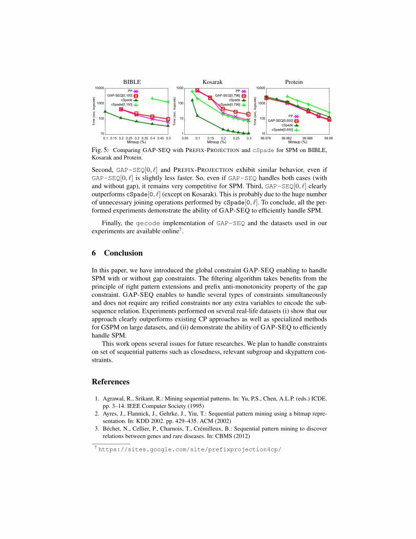
(e) Evaluating the ability of GAP-SEQ to efficiently handle SPM. In order to sim-ulate the absence of gap constraints, we used the ineffective gap[0, `] constraint (recallthat ` is the size of the longest sequence of SDB). We compared GAP-SEQ[0, `] withPREFIX-PROJECTION and two configurations of cSpade for SPM: cSpade withoutgap constraint and cSpade with M and N set respectively to 0 and `, denoted bycSpade[0, `]. Let us note that all the above methods will extract the same set of sequen-tial patterns.

Fig. 5 reports the CPU times for the four methods. First, cSpade obtains thebest performance (except on Protein). These results confirm those observed in [7].

BIBLE Kosarak Protein

10

100

1000

10000

0.1 0.15 0.2 0.25 0.3 0.35 0.4 0.45 0.5

Tim

e (

sec, lo

gscale

)

Minsup (%)

PP

GAP-SEQ[0,100]

cSpade

cSpade[0,100]

1

10

100

1000

0.05 0.1 0.15 0.2 0.25 0.3

Tim

e (

sec, lo

gscale

)

Minsup (%)

PP

GAP-SEQ[0,796]

cSpade

cSpade[0,796]

10

100

1000

10000

99.978 99.982 99.986 99.99

Tim

e (

sec, lo

gscale

)

Minsup (%)

PP

GAP-SEQ[0,600]

cSpade

cSpade[0,600]

Fig. 5: Comparing GAP-SEQ with PREFIX-PROJECTION and cSpade for SPM on BIBLE,Kosarak and Protein.

Second, GAP-SEQ[0, `] and PREFIX-PROJECTION exhibit similar behavior, even ifGAP-SEQ[0, `] is slightly less faster. So, even if GAP-SEQ handles both cases (withand without gap), it remains very competitive for SPM. Third, GAP-SEQ[0, `] clearlyoutperforms cSpade[0, `] (except on Kosarak). This is probably due to the huge numberof unnecessary joining operations performed by cSpade[0, `]. To conclude, all the per-formed experiments demonstrate the ability of GAP-SEQ to efficiently handle SPM.

Finally, the gecode implementation of GAP-SEQ and the datasets used in ourexperiments are available online7.

6 Conclusion

In this paper, we have introduced the global constraint GAP-SEQ enabling to handleSPM with or without gap constraints. The filtering algorithm takes benefits from theprinciple of right pattern extensions and prefix anti-monotonicity property of the gapconstraint. GAP-SEQ enables to handle several types of constraints simultaneouslyand does not require any reified constraints nor any extra variables to encode the sub-sequence relation. Experiments performed on several real-life datasets (i) show that ourapproach clearly outperforms existing CP approaches as well as specialized methodsfor GSPM on large datasets, and (ii) demonstrate the ability of GAP-SEQ to efficientlyhandle SPM.

This work opens several issues for future researches. We plan to handle constraintson set of sequential patterns such as closedness, relevant subgroup and skypattern con-straints.

References

1. Agrawal, R., Srikant, R.: Mining sequential patterns. In: Yu, P.S., Chen, A.L.P. (eds.) ICDE.pp. 3–14. IEEE Computer Society (1995)

2. Ayres, J., Flannick, J., Gehrke, J., Yiu, T.: Sequential pattern mining using a bitmap repre-sentation. In: KDD 2002. pp. 429–435. ACM (2002)

3. Béchet, N., Cellier, P., Charnois, T., Crémilleux, B.: Sequential pattern mining to discoverrelations between genes and rare diseases. In: CBMS (2012)

7 https://sites.google.com/site/prefixprojection4cp/

4. Coquery, E., Jabbour, S., Saïs, L., Salhi, Y.: A SAT-based approach for discovering frequent,closed and maximal patterns in a sequence. In: ECAI. pp. 258–263 (2012)

5. Fournier-Viger, P., Gomariz, A., Gueniche, T., Soltani, A., Wu, C., Tseng, V.: SPMF: A JavaOpen-Source Pattern Mining Library. J. of Machine Learning Resea. 15, 3389–3393 (2014),http://jmlr.org/papers/v15/fournierviger14a.html

6. Ji, X., Bailey, J., Dong, G.: Mining minimal distinguishing subsequence patterns with gapconstraints. In: (ICDM’05. pp. 194–201 (2005)

7. Kemmar, A., Loudni, S., Lebbah, Y., Boizumault, P., Charnois, T.: PREFIX-PROJECTIONglobal constraint for sequential pattern mining. In: Principles and Practice of Constraint Pro-gramming - 21st International Conference, CP 2015, Cork, Ireland, August 31 - September4, 2015, Proceedings. pp. 226–243 (2015)

8. Kemmar, A., Ugarte, W., Loudni, S., Charnois, T., Lebbah, Y., Boizumault, P., Crémilleux,B.: Mining relevant sequence patterns with cp-based framework. In: ICTAI. pp. 552–559(2014)

9. Li, C., Wang, J.: Efficiently mining closed subsequences with gap constraints. In: SIAM2008 on Data Mining. pp. 313–322 (2008)

10. Li, C., Yang, Q., Wang, J., Li, M.: Efficient mining of gap-constrained subsequences and itsvarious applications. Trans. Knowl. Discov. Data 6(1), 2:1–2:39 (Mar 2012)

11. Métivier, J.P., Loudni, S., Charnois, T.: A constraint programming approach for mining se-quential patterns in a sequence database. In: ECML/PKDD Workshop on Languages for DataMining and Machine Learning (2013)

12. Négrevergne, B., Guns, T.: Constraint-based sequence mining using constraint programming.In: CPAIOR’15. pp. 288–305 (2015)

13. Pei, J., Han, J., Mortazavi-Asl, B., Pinto, H., Chen, Q., Dayal, U., Hsu, M.: PrefixSpan: Min-ing sequential patterns by prefix-projected growth. In: ICDE. pp. 215–224. IEEE ComputerSociety (2001)

14. Wu, X., Zhu, X., He, Y., Arslan, A.N.: PMBC: pattern mining from biological sequenceswith wildcard constraints. Comp. in Bio. and Med. 43(5), 481–492 (2013)

15. Yang, G.: Computational aspects of mining maximal frequent patterns. Theor. Comput. Sci.362(1-3), 63–85 (2006)

16. Zaki, M.J.: Sequence mining in categorical domains: Incorporating constraints. In:CIKM’00. pp. 422–429 (2000)

17. Zaki, M.J.: SPADE: An efficient algorithm for mining frequent sequences. Machine Learning42(1/2), 31–60 (2001)

18. Zhang, M., Kao, B., Cheung, D.W., Yip, K.Y.: Mining periodic patterns with gap requirementfrom sequences. TKDD 1(2) (2007)