FACOLTA DI SCIENZE E TECNOLOGIE

Corso di Laurea Triennale in Fisica

L’integrale di Feynmanper particelle in campo elettromagnetico

CODICE PACS: 03.65.-w

Candidato:

Francesco BORRA794134

Relatore:

Prof. Luca Guido MOLINARI

Anno Accademico 2013-2014

Contents

I Formulation of the Path Integral 4

1 Motivation 4

2 Propagator 5

3 Position representation and Trotter Product 6

4 The Wiener measure and the nature of Feynman paths 10

5 Vector potential 14

6 Phase Space 17

7 Coherent states representation 18

II Applications and examples 24

8 Hamiltonian spectrum 24

9 Free Particle 24

10 Quadratic Lagrangians and classical trajectories 26

11 Uniform electric field 28

12 Harmonic Oscillator 29

13 Uniform magnetic field 30

III The Aharonov Bohm e↵ect - a topological approach 34

14 Motivation 34

15 Path Integral on multiply connected spaces 36

16 Aharonov-Bohm e↵ect on the circle 40

17 Aharonov-Bohm e↵ect on the plane 42

18 Experimental evidence 45

19 Interpretation 50

2

A Appendix: minimal homotopy theory 51

3

Part I

Formulation of the Path Integral

1 Motivation

Feynman proposed a formulation of quantum mechanics which is alternativeto the familiar Hilbert space one. In this section, the main ideas will beroughly outlined.

The starting point is the attempt to determine the probability to find aparticle at some point B, assuming that it was localized at some other pointA before. As it is known from the double slit experiment and its variants,in quantum mechanics exclusive alternatives can interfere. The “exclusivealternatives” in this case are all the possible trajectories connecting the twopoints. Yet, a proper definition of trajectory is troublesome in quantummechanics as it is not possible to define the position of a particle at anygiven time. Nevertheless, it is possible to proceed as follows.

An impenetrable surface can be interposed between the two points. Thesurface has some holes with detectors or other devices that can perform ameasure process. Anytime the particle passes through a hole, the alterna-tives collapse and the particle proceeds beyond the surface from the hole,so that the position of the particle can be specified in one point. If severalsimilar surfaces are interposed, then the position is well defined at someinstants and at some points which form a sort of path. In the limit of manysurfaces and many holes - which means no surfaces and no holes - the par-ticle moves along a sort of trajectory which can be regarded as one of themutually exclusive alternatives.

In classical mechanics, the probability that the particle reaches B wouldbe the sum of the probabilities of the independent trajectories. In quantummechanics, according to the previous picture, there are paths and they areallowed to interfere if all the detectors are turned o↵. The quantity thataccounts for the interference is the phase. No path is more important thanthe others but each one carries a di↵erent phase. The square modulus of theirsum can be interpreted as a probability. The phase will be some functionof the trajectory and the correct choice is exp [(i/~)S(x(t))] where S is theclassical action associated with the trajectory.

The sum of the phases is then:

g(xf , tf ;xi, ti) =Xpaths

exp [(i/~)S(x(t))]

The quantity |g(B, t;A, 0)|2 is the probability that the particle reaches Bafter a time t. Yet, as in quantum mechanics the position is never free ofuncertainty, a better definition of probability should involve a proper initial

4

physical state and not just an initial position. Since trajectories are expectedto be a continuous set rather than a countable one, it would be interestingto be able to write an integral instead of a sum.

A more rigorous approach to the problem will follow. A quantity calledpropagator will be introduced and it will be shown to yield the function gwhich has just been investigated. In addition, the propagator, as a moreabstract object, will allow the extension the previous path approach to tra-jectories which belong to di↵erent spaces and not just the configurationspace.

2 Propagator

Given a linear di↵erential operator L, the Green function g(x) has the fol-lowing property: Lg(x) = �(x)

Similarily, the propagator G can be defined for the Schrodinger equation(S.E.) as a sort of Green function, with the only di↵erence that G is anoperator.

(H � i~@t)G(t, t0

) = �i~�(t� t0

) (1)

Given a state-vector at a certain time t0

, the propagator yields its evolutionthrough time for t > t

0

:

| (t)i = G(t, t0

) | (t0

)i

Indeed, G(t, t0

) | (t0

)i is a solution of S.E. for t 6= t0

, since

(H � i~@t)G(t, t0

) | (t0

)i = �i~�(t� t0

) | (t0

)i

Therefore, G(t, t0

) is “almost” the time-evolution operator U(t, t0

) and pre-cisely ✓(t� t

0

)U(t, t0

) which can be directly verified, considering the Leibnizproperty and that d

dt✓(t� t0

) = �(t� t0

).If the Hamiltonian is time-independent, then:

G(t, t0

) = ✓(t� t0

)e�iH~ (t�t0) (2)

The ✓ function will be omitted when not explicitly needed.The propagators form a semi-group with the following properties:

• G(t, t0

) = 0 if t < 0

• G(t2

, t1

)G(t1

, t0

) = G(t2

, t0

)

• G(t, t) = I

5

If H is time-independent, the propagator only depends on the di↵erenceof times t and t

0

and, consequently, it is invariant under time translation.With an abuse of notation, one can write G(t, t

0

) = G(t � t0

). Thus, fromnow on, t

0

will be set to zero. It must be remarked that in literature theterm “Green function” is often referred to the Fourier transform of G, i.e.the energy-dependent propagator.

3 Position representation and Trotter Product

The position representation is the kernel of G(t, t0

):

(y, t) = hy|G(t, t0

) | (t0

)i=

Zdx hy|G(t, t

0

) |xi hx| (t0

)i

=

ZdxG(y, t;x, t

0

) (x, t0

)

The goal is to find an explicit expression for the kernel G(y, t;x, t0

).

Let us consider the simple case of a potential which only depends onthe position. The Hamiltonian reads H = p2/2m + V (x). Since, in theend, time evolution will appear as a succession of events, we can split thetime interval t := t � t

0

into N sub-intervals and, recalling the semi-groupproperties, re-write G as a product (the ✓ function will be omitted):

e�it~ H =

he�

itN~H

iNThe next step is to separate the momentum from the position i.e. thepotential from the kinetic part. This is a delicate passage since V and p2 donot commute. If two operators, say A and B, commute then eAeB = eA+B

according to the Baker-Campbell-Hausdor↵ formula. In the present case,according to the same formula, the best we can obtain is:

e�itN~ (T+V ) = e�

itN~V e�

itN~T + o(N�1)

where by definition an operatorR(h) = o(h) if 8 | i 2 H limh!0

||R(h) | i ||/h !0. Hence, the product of N propagators reads:

e�it~ H = [e�

itN~V e�

itN~T + o(N�1)]N

If N is big enough, one can hope to neglect the terms o(N�1) in the previousexpression. This possibility is o↵ered by the Trotter formula, which will bepresented in the following simplified version:

8 | i 2 H limN!1

(eA/NeB/N )N | i = eA+B | i (3)

6

with some operators A and B. Obviously the formula is true only under somerestrictive hypotheses on A and B and there are domain issues too. Thedetails will not be discussed here, but the main result1 is that if A ⇠ p2/2m,B ⇠ V (x) (a “well-behaved” potential) and p2/2m+ V = H is self-adjoint,then the Trotter product is valid. Consequently, an operator which is welldefined as an Hamiltonian for ordinary quantum mechanics, should also befine in the current description. Finally:

G(y, t;x) = limN!1

hy| [e� itN~T e�

itN~V ]N |xi

Since the potential V only depends on the position V=V(x), V itself and

its exponential are diagonal in the position basis, such as T = ~2k22m and

its exponential are diagonal in the impulse basis. It is useful to insert theidentity operator

Rdx |xi hx| between every couple of consecutive terms in

the previous equation.

G(y, t;x) = limN!1

Zdx

1

...dxN�1

N�1Yj=0

hxj+1

| e� itN~T e�

itN~V |xji (4)

Each term of the product can be rewritten this way:

hxj+1

| e� itN~T e�

itN~V |xji = hxj+1

| e� itN~T |xji e� it

N~V (xj)

= hxj+1

| e� itN~T

Zdk |ki hk|

�|xji e� it

N~V (xj)

= e�itN~V (xj)

Zdk hxj+1

|ki hk|xji e� itN~

~2k2m

=1

2⇡~e� it

N~V (xj)

Zdk e�

itN~

~2k22m +

ik~ (xj+1�xj) (5)

Now one can either integrate over k or just rearrange the new expression.The latter procedure will be discussed in the section about the phase-space,whereas the former approach will follow here. The integral above is Gaussianand its value is r

mN

2i⇡t~e�mN(xj+1�xj)

2/it~

Hence, each factor in equation (4) is the product of two exponentials. Theproduct is conveniently rewritten as the exponential of a sum. With a smallrearrangement, one gets the following meaningful result:

limN!1

m

2i⇡~(t/N)

�N/2 Zdx

1

...dxN�1

⇥

⇥ exp

24 i(t/N)

~

N�1Xj=0

"m

2

(xj+1

� xj)

t/N

�2

� V (xj)

#35 (6)

1There exist more than one su�cient condition for the Trotter product

7

The sum in the exponent resembles the definition of a Riemann integral asN goes to infinity and t/N goes to zero.

t

N

N�1Xj=0

m

2

(xj+1

� xj)2

t/N� V (xj)

�⇡Z t

0

dt0"m

2

dx(t0)

dt0

�2

� V (x(t0))

#(7)

Nevertheless, the sum is not a genuine Riemann integral since the limit istaken after the integration and, in general, it is not even true that xj �xj�1

should go to zero as t/N ! 0. This issue will be one of the main topics ofthe next section.

The integrand in (7) is what in classical mechanics is called Lagrangian;therefore its integral with respect to time is an analogue of the classicalaction.

S(t) =

Z t

0

dt0L(t0)

The discrete version of S is sometimes called “sliced action” since Ssliced =PS(xj , xj+1

). If N is fixed, the N integrals may be thought of as a “sum”

of ei~S(x(·)) over any possible broken line path connecting N points, while

keeping the first and the last points fixed, as well as the time interval t.As N increases, seemingly-continuous successions of points appear and thesum-over-paths interpretation becomes even more reasonable. Finally, if Cis the normalization constant, the following formula can be written:

G(xf , t;xi) = CXx(·)

x(0)=xi

x(t)=xf

ei~S(x(·)) (8)

This “sum” over paths can be interpreted as an integral on the “set of allpaths” satisfying the conditions above: a path integral. It is importantto underline that, in order to define an actual integral, a proper measure isnecessary and that in the present section no “bona fide measure” is presented[27]. Thus, however simple the previous and the next expressions might be,they make sense according to (6).

G(xf , t;xi) =

Z xf

xi

Dx(t) exp

it

~ S(x(t))�

(9)

The previous formalism has been derived in one dimension but it canalso apply to systems with several degrees of freedom. Let us consider, forexample, a particle moving in R3. We write

G(xf

, t;xi

) =

Z xf

xi

Dx(t)Dy(t)Dz(t) exp

it

~ S(x(t), y(t), z(t))�

(10)

as a formal expression for a multi-dimensional generalization of (6). If theaction can be split in a sum in which each addend depends on di↵erent set

8

of variables, the system is separable. The integrations over the independentcoordinates can be divided and it is straightforward that:

S(x1

,x2

) = S1

(x1

) + S2

(x2

)

) G(x1,f ,x1,f , t;x2,i,x1,i) = G(x

1,f , t;x1,i)G(x2,f , t;x2,i).

Let us note that | h�| (t)i |2 = | h�|G | i |2 is the transition probabilityfrom | i to |�i after the former has evolved for a time t. If now the twostates are :

| i 7! |xii |�i 7! |xf iit follows that

|G(xf , t;xi)|2 (11)

is precisely the probability that a particle localized at xi is detected at xf attime t: the search of such probability has been the introductory argumentfor the path integral. It must be remarked that if | i is exactly |xii theprobability distribution is quite strange (38) and, in order to get a morephysical result, it is better to consider an appropriate initial state (e.g. acoherent state) which is localized but which is not a position eigenvalue. Ifsuch state is |

xii then:

P (xf

, t;xi

) =

����Z d3xG(xf , t;xi) xi(x)

����2Finally, the composition property of propagators (as elements in a semi-

group) can be rewritten in the position representation. Let us fix an inter-mediate time tm such that 0 < tm < t.

G(xf , t;xi) = hxf |G(t, tm)G(tm, 0) |xii= hXf |G(t, tm)

Zdxm |xmi hxm|G(tm, 0) |xii

=

ZdxmG(xf , t;xm, tm)G(xm, tm;xi, 0).

The previous integral is interpreted as a sum over all possible intermediatepositions a time tm and this means that the amplitude of “events occurringin succession” multiply.

With an abuse of terminology, from now on, the kernel will be simplyreferred to as the “propagator”.

9

4 The Wiener measure and the nature of Feynmanpaths

The trajectories appearing in the path integral can in principle assume anypossible shape. Even in the N ! 1 limit, there can be arbitrarily bigdistances between two successive vertices on the broken lines. Nevertheless,some paths are expected to be more meaningful then others (i.e. give themost significant contribution to the sum). Therefore, it is useful to studywhat the typical quantum path “looks like”.

In order to reach this goal, it is worth considering the classical analogueof the path integral i.e. the Brownian motion, or “random walk” along withthe Wiener measure. This insight sheds some light on some points.

First, it clarifies what the path integral is not: an integral in strictlymathematical terms, or at least not in a straightforward way, whereas theclassical Wiener integral is. Therefore, it becomes clearer which propertiesare lost (or gained) after the quantization.

Second, the analogy with Brownian motion is a possible way to guesssome physical properties of the path. In particular, the knowledge of therelationship between the typical length of a “jump” and its timespan willallow to compare infinitesimal quantities in the short-time limit and thus torecover Schrodinger equation from the path integral which is the ultimateway of checking its consistency.

Let us consider a particle at some point x

0

in space, moving to a newposition at a fixed distance ` but in a random direction at regular timeintervals ✏. After the first step, the probability of the particle being in aninfinitesimal neighbourhood d3x of certain position x is:

P (x|x0

)d3x =1

4⇡`2�(|x� x

0

|� `)d3x

Since P (x0|x) is only a function of x0 �x, the probability distribution afterN steps can be expressed as a convolution product, i.e. as a conditionalprobability. Given the N � 1 step distribution and a fixed x

0

:⇢P (x

1

, 1) = 1

4⇡`2�(|x

1

� x

0

|� `)P (x, N) =

Rd3x0P (x|x0)P (x0, N � 1)

By applying the Fourier transform FP (k, N) = (FP (k, 1))N and consider-ing that FP (k, 1) = sin k`

k` , then:

FP (k, N) =

sin k`

k`

�N⇡1� (k`)2

6

�N⇡ exp

�N(`k)2

6

�The previous approximation is justified under the hypothesis that N ! 1and `! 0 while the exponential remains finite, i.e. `2N is finite. Let x

0

= 0;

10

after taking the anti-transform, the final result is:

P (x, N) =

2⇡N`2

3

�� 32

exp

� 3x2

2N`2

�Time can be explicitly introduced in the previous formula by calling ✏N =t� t

0

. Few additional substitutions yield

⇢(x, t;x0

, t0

) := P (x, t;x0

, t0

) =

1

4⇡D(t� t0

)

� 32

exp

� (x� x

0

)2

4D(t� t0

)

�(12)

The previous probability distribution describes a di↵usion process governedby a parameter D = `2/6✏, which in the case of classical Brownian motiondepends on the medium. Before moving to the next passage it is useful tonotice that ⇢ satisfies the heat equation:✓

@

@t�Dr2

◆⇢(x, t;x

0

, t0

) = 0 (13)

where for simplicity we consider t > t0

and x 6= x

0

Incidentally, let usobserve that limt!t0 ⇢(x, t;x0

, t0

) = �3(x� x

0

).Now that the probability of a particle moving from one region of space

to another has been determined, a measure for the space of paths can bedefined. Let us consider a partition of the time interval t � t

0

, namely{t

0

, t1

, ...tN}, and an equal number of Borel sets Ik ⇢ R3. The probabilitythat a particle travelling from x

0

to x

N

passes through the region Ik attime tk (i.e. x(tk) 2 Ik) is almost :

m(x, t;x0

, 0) =

ZI1

d3x1

ZI2

d3x2

...

ZIN�1

d3xN�1

⇥

⇥ ⇢(x1

, t1

;x0

, t0

)⇢(x2

, t2

;x1

, t1

)...⇢(xN

, tN ;xN�1

, tN�1

) (14)

It is “almost” a probability because the conditioned probability is P (A|B) =P (A ^ B)/P (B). As a consequence, to recover a proper probability oneshould divide the previous formula by ⇢(x, t;x

0

, t0

). Alternatively, if theend-point is not fixed, i.e. if one integrates over the last variable, one gets anon-conditional probability.

As N ! 1 the motion of the particle is described by a broken linetrajectory just as those appearing in the path integral. The chance of bigjumps drops exponentially and the big-N limit suggests that the successionof the vertices should appear as a continuous curve if the tj � tj�1

! 0accordingly. Yet, there is no guarantee of di↵erentiability.

The previous description makes it possible to define the Wiener measurein the space of paths for a Brownian particle. The basic results will be listedbelow.

11

• W(x, t;x0

, t0

) is the set of continuous curves connecting x

0

and x ina time interval t� t

0

.

• “Cylindrical sets” are defined as the sets of paths

K(t0

,x0

; t1

, I1

; ...; tN�1

, IN�1

; tN ,xN

),

i.e. the set of trajectories passing through Ik at tk as described above.All Ks, their complements, their countable unions and finite intersec-tions constitute the �-algebra.

• A positive measure for K can be defined as the conditional-probabilityof the particle moving along one of the paths in K. Then µ(K) can bedefined as (14) either normalized or not.

The properties above identify a proper positive measure: the conditionalWiener measure. By choosing a set IN for the last step instead of fixing thefinal point, the non-conditional Wiener measure can be found.

A functional is a function Q : W(x, t;x0

, 0) 7! R. Q can be integrated:

hQi =Z

dµ(x(⌧))Q(x(⌧)) (15)

In practice, hQi can be evaluated like the path integral: one integrates Qover broken lines with N vertices after setting tj � tj�1

= (t � t0

)/N = ✏,and finally lets N ! 1. Hence, in the discrete form, one gets:

dµ(x(t)) 7!Y d3x

j

(4⇡D✏)3/2exp

✓�(xj+1

� xj)2

4D(✏/N)

◆(16)

andQ(x(t)) 7! Q(x

0

,x1

, ...,xN )

The integral (15) is almost an average of the quantity Q over all possiblepaths. Again, it is almost an average because it is not normalized. This factis clearer if one considers the functional 1 : x(t) 7! 1 i.e. if one evaluatesthe “volume” of the space of all paths.

h1i = µ(W(x, t;x0

, 0)) =

Zdµ(x(⌧)) = ⇢(x, t;x

0

, 0) 6= 1

The previous formulas highlights certain similarities between the Wienerintegral and the position representation of the propagator. Keeping this inmind, let us observe that expression (16) introduces a sort of kinetic termin the exponent; therefore, in order to make a connection with Feynmanintegral, it is natural to consider a functional that somehow accounts for thepotential:

F = exp

ZdtU(x(t))

�12

for some U(x). The average of F has a familiar form:

J =

Zdµ(x(t)) exp

�Z

d⌧U(x(⌧))

�(17)

or, even more explicitly:

J = limN!1

1

4⇡D✏

� 3N2Z N�1Y

j=1

d3xj exp

"N�1Xk=0

✓�(xk+1

� xk)2

4D✏� U(xk)

◆#(18)

It can be shown that the new quantity J satisfies a modified heat equation:

@

@tJ = Dr2J � U(x)J (19)

This equation resembles that of the quantum propagator (1), just like theexpression for J is quite similar to G. There is indeed a correspondence:

D $ i~m

U $ i

~V ) J $ G

(19) corresponds to S.E. up to a delta which arises immediately from allowingt� t

0

to be negative (J = 0 if t < t0

). Therefore, the path integral looks likean analytic continuation of the Wiener integral. One may want to regardthe path integral as more than a sort of complex average of the functionalexp

⇥i~RdtL⇤. The idea would be to define a complex measure for Feynman

paths as

dµ(x(t)) = Dx(t) exp

i

~

Zd⌧

m

2x

2

�maybe in its discrete form. Unfortunately, as the complexification takesplace, a well-defined measure is lost: while in general it is possible to definecomplex measures, the complexified Wiener measure is not countably addi-tive [17].

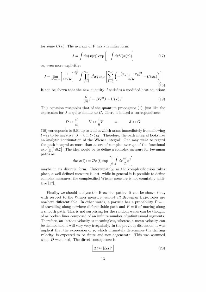
Finally, we should analyse the Brownian paths. It can be shown that,with respect to the Wiener measure, almost all Brownian trajectories arenowhere di↵erentiable. In other words, a particle has a probability P = 1of travelling along nowhere di↵erentiable path and P = 0 of moving alonga smooth path. This is not surprising for the random walks can be thoughtof as broken lines composed of an infinite number of infinitesimal segments.Therefore, an instant velocity is meaningless, whereas a mean velocity canbe defined and it will vary very irregularly. In the previous discussion, it wasimplicit that the expression of ⇢, which ultimately determines the driftingvelocity, is expected to be finite and non-degenerate. This was assumedwhen D was fixed. The direct consequence is:

�t ⇡ |�x|2 (20)

13

In other words, finite displacements cannot occur in an infinitesimal times-pan and “big jumps” are forbidden. The close resemblance to Feynmanintegral suggests that quantum paths should be alike. It should be said thata naive extension of (20) to quantum path may be questionable and thereare other methods and approximations that yield (20) for Feynman pathsunder more general hypotheses and that do not involve Brownian motion.This last relation (20) is especially important and it will be used again. Inparticular, (20) implies that, in the path integral, the velocity is not welldefined as a limit, since �x/�t ! 1, or, equivalently, given two vertices jand j + 1 in (6), then (xj+1

� xj)/(t/N) ! 1 (as anticipated, the nowheredi↵erentiability already accounts for this).

5 Vector potential

The path integral has been obtained from the Trotter formula under the hy-pothesis that the potential is only dependent on the position. This excludesmagnetic fields from the description. In order to introduce them, it is rea-sonable to simply introduce an electromagnetic potential in the Lagrangianin (8). The classical electromagnetic Lagrangian is:

L =m

2

dx

dt

�2

� V (x) +e

c

dx

dtA(x)

In the path integral formalism, its integral (the Sliced action) should beevaluated according to (7), as followsZ t

0

dt0e

c

dx

dt0A(x(t0)) =

e

c

Zx(·)

dxA(x) =:e

c

N�1Xj=0

(xj+1

� xj)A(x(j, j + 1))

x(j, j + 1) is the point in which the vector potential is evaluated in eachstep and it should be some point on the segment connecting xj and xj+1

.This choice would be of no concern if Riemann integration theory could beapplied: any choice, e.g. xj or xj+1

, would be appropriate. But this is astochastic integral (Ito’s theory [28]), not a Riemann integral, and the onlycorrect choice will be xj+1+xj

2

as will be shown later.The correctness of the previous guess can be verified by checking that, in

an infinitesimal time interval, the propagator yields the same time evolutionas the Schrodinger equation. Since the path integration describes the evolu-tion as a succession of steps, only the first step will be kept and its timespanwill be assumed infinitesimal. According to (20), also �x is infinitesimaland its relation with �t is fixed. Let us evaluate the vector potential at

14

some point xf + ↵(xi � xf ), ↵ 2 [0, 1].

(xf , t) =⇣ m

2i⇡~t

⌘3/2Z

d3xi (xi, 0)⇥

⇥ exp

it

~

"m

2

xf � xi

t

�2

� V (x) +e

c(xf � xi)A(xf + ↵(xi � xf ))

#!(21)

The purpose of the following passages is to get a first-order (in t) approxi-mation of the previous expression. Let xi � xf = ⇠, then

(xf , t) =

Zd3⇠

⇣ m

2i⇡~t

⌘3/2

exp

✓im⇠2

2~t

◆⇥

⇥ exp

✓� it

~ [V (xf )�rnV (xf )⇠n] + o(t)

◆⇥

⇥ exp

✓� ie

~c⇠n [An(xf ) + ↵(⇠krk)An(xf )] + o(t)

◆⇥

⇥ (xf , 0) + ⇠nrn (xf , 0) +

1

2⇠m⇠k

@2

@xm@xk(xf , 0) + o(t)

�The exponentials can expanded in series. Since all quantities in the followingequation are evaluated in xf , the spatial dependence will be omitted.

(t) =⇣ m

2i⇡~t

⌘3/2✓1� it

~ V◆Z

d3⇠ exp

✓im⇠2

2~t

◆⇥

1� ie

~c⇠nAn � ↵ie

~c⇠n⇠mrmAn � e2

2~2c2 ⇠n⇠kAnAk

�⇥

⇥ (xi, 0) + ⇠nrn (xi, 0) +

1

2⇠m⇠k

@2

@xm@xk

�+ o(t) (22)

In the previous integral, all odd terms (i.e. those that are linear at least inone ⇠k) vanish and the only integrals that are left have the following forms:Rx2e�ix2

orRe�ix2

. After some rearrangements, one gets:

i~ =

✓� ~22m

r2 +e2

2mc2A2 + ↵

ie~mc

(r ·A) +ie~mc

(A ·r) + V

◆

= � ~22m

r2 +e2

2mc2A2 + (↵� 1/2)

ie~mc

(r ·A) +

+ie~2mc

(A ·r) +ie~2mc

r · (A ) + V

where @ @t = ( (t)� (0))/t which is true for t ! 0. If we want the previous

equation to be the Schrodinger equation, the only possible choice of ↵ is↵ = 1/2 and this fact is called “mid-point” rule.

15

There is no mid-point rule for the scalar potential V and any pointx(j, j + 1) on the segment [xj ,xj+1

] would yield the correct result. Thereason is that, in the series expansion of V (x) about some x(j, j + 1), theonly term which remains is V (x(j, j+1)) since it is zero order in ✏ = t/N : inthe sliced action, V is multiplied by ✏ and, consequently, the error derivingfrom changing the evaluation point (order ✏1/2) is always neglectable. Onthe other hand, the vector potential is multiplied by xj+1

� xj which is oforder ✏1/2 and thus the error introduced by the change of evaluation point(✏1/2 again) cannot be neglected since the overall error goes as ✏. Physicallyspeaking, the vector potential is coupled to the “velocity” which is a highlyoscillating quantity in Brownian-like paths and therefore the situation ismore delicate.

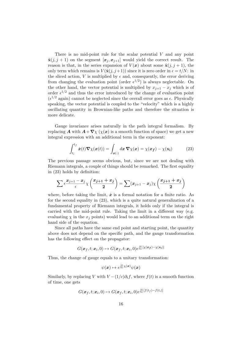
Gauge invariance arises naturally in the path integral formalism. Byreplacing A with A+r� (�(x) is a smooth function of space) we get a newintegral expression with an additional term in the exponent:Z tf

ti

x(t)r�(x(t)) =

Zx(·)

dxr�(x) = �(xf

)� �(xi

) (23)

The previous passage seems obvious, but, since we are not dealing withRiemann integrals, a couple of things should be remarked. The first equalityin (23) holds by definition:X

✏xj+1

� xj

✏�

✓x

j+1

+ x

j

2

◆=X

(xj+1

� xj)�

✓x

j+1

+ x

j

2

◆where, before taking the limit, x is a formal notation for a finite ratio. Asfor the second equality in (23), which is a quite natural generalization of afundamental property of Riemann integrals, it holds only if the integral iscarried with the mid-point rule. Taking the limit in a di↵erent way (e.g.evaluating � in the xj points) would lead to an additional term on the righthand side of the equation.

Since all paths have the same end point and starting point, the quantityabove does not depend on the specific path, and the gauge transformationhas the following e↵ect on the propagator:

G(xf , t;xi, 0) 7! G(xf , t;xi, 0)eie~c [�(xf )��(xi)]

Thus, the change of gauge equals to a unitary transformation:

(x) 7! eie~c�(x) (x)

Similarly, by replacing V with V �(1/c)@tf , where f(t) is a smooth functionof time, one gets

G(xf , t;xi, 0) 7! G(xf , t;xi, 0)eie~c [f(tf )�f(ti)]

16

since Z tf

ti

dt @tf(t) = f(tf )� f(ti)

reasonably holds for the sliced integral. Again, f(tf ) and f(ti) are the samefor all paths. In the general case, let ⇤(x, t) be a function of both space andtime. The gauge transformation becomes

A 7! A+r⇤ V 7! V � 1

c@t⇤

Thus, sinceZdt [@t⇤(x(t), t) + x(t)r⇤(x(t), t)] =

Zdt

d

dt⇤(x(t), t) = ⇤(xf , tf )�⇤(xi, ti)

one gets again

G(xf , t;xi, 0) 7! G(xf , t;xi, 0)eie~c [⇤(xf ,tf )�⇤(xi,ti)].

6 Phase Space

As anticipated during the derivation of the position representation, if theintegrals over impulses are not performed, additional N variables are kept.

G(xf , t;xi, 0) = limN!1

Z NYj=1

dkj2⇡~

N�1Yl=1

dxl

exp

24 i

~

NXq=1

"t

N

k2q2m

+ V (xq)

!+ kq(xq � xq�1

)

#35 (24)

The exponential in the previous integral can be formally written as:

exp

i

~

Zdt (px�H(x, p))

�The previous expression recalls the Hamiltonian formalism in classical me-chanics which allows defining a class of canonical variables and a way to passfrom one to the other. Yet, in general, classical results cannot be extendedto the path integral formalism [28].Quantum trajectories in phase space are not smooth and not even Brownian-like. Furthermore, a classical trajectory in the phase space is completelyidentified by the law of motion x(t) which fixes p(t). However, if, beforetaking the limit, (24) is interpreted as a sum of broken-lines paths withN steps, between each couple of vertices xi�1

and xi the momentum is re-dundantly specified by ki. Thus the motion is not classical and p(t) hasdiscontinuities at each vertex. Another interpretation is possible: the timet is divided into 2N intervals. The motion is classical and at each vertexeither the position or the momentum are alternatively specified.

17

7 Coherent states representation

Coherent states can be defined in a rather general fashion as a set of vectorsin the Hilbert space H satisfying certain conditions. Namely, they mustbe both the images of elements from some “label-set” L under a stronglycontinuous map and they must yield a resolution of unity

RL dl |li hl| with dl

being an appropriate measure. From now on, canonical coherent states willbe examined and they will be referred to simply as coherent states.

Canonical coherent states can be either defined as eigenstates of the low-ering operator a = q+ipp

2~ or as minimum uncertainty states. Some definitions

are needed. The eigenstates of the harmonic oscillator can be labelled withintegers |ni. Then:

a |ni = pn |n� 1i

a† |ni = pn+ 1 |n+ 1i

[a, a†] = 1

a |0i = 0

Let now |zi be a vector such that

a |zi = z |zi

and let us expand it on the |ni basis.

zXn

µn |ni = z |zi = a |zi = aXn

µn |ni

=X

µn

pn |n� 1i =

Xµn+1

pn+ 1 |ni

zµn =pn+ 1µn+1

implies that µn = znpn!µ0

. µ0

can be determined by

imposing 1 = hz|zi. The result is:

|zi = exp

� |z|2

2

�Xn

znpn!

|ni

It follows that

hw|zi = exp

� |w|2 + |z|2

2+ w⇤z

�An equivalent form will be used later:

hw|zi = exp⇥�1

2

[w⇤(w � z)� z(w⇤ � z⇤)]⇤

(25)

There is another characterization of coherent states. They are harmonicoscillator ground states displaced both in space and momentum. Let T⇠1

18

and D⇠2 be the corresponding displacement operators. It will be shown that

z = ⇠1+i⇠2p2~ :

aT⇠1D⇠2 |0i = T⇠1D⇠2T†⇠1D†⇠2aT⇠1D⇠2 |0i

= T⇠1D⇠2

✓⇠1

+ i⇠2p

2~+ a

◆|0i

=

⇠1

+ i⇠2p

2~

�T⇠1D⇠2 |0i

If we define |zi = T⇠1D⇠2 |0i, some properties follow directly from the obser-vations above:

hz| q |zi = <(z)p2~

hz| p |zi = =(z)p2~

�p�q = h0| q2 |0i h0| p2 |0i = ~2

Hence, the minimum uncertainty property has been proved. It is also truethat any minimum uncertainty state is a coherent state.

The wavefunction associated with |zi can be evaluated as T⇠1D⇠2 |0i.The Schrodinger representation for |0i is ⇡1/4 exp(�x2/2). Then:

z(x) = ⇡�1/4 exp

✓i⇠

2

x

~

◆exp

✓�(x� ⇠

1

)2

2~

◆Then, up to the irrelevant constant phase factor exp(i⇠

1

⇠2

/~), the wavefunc-tion can be written as:

z(x) = ⇡�14 exp

� |z|2

2� x2 + z2

2+

p2zx

�The coherent states allow to define a basis of vectors. Yet, their set C ={|zi : z 2 C} is overcomplete and, consequently, the resolution is not unique.The subset B ⇢ C, defined as B = {|wi 2 C : w = m + in;m,n 2 Z} is apossible nontrivial complete set [3]. More in general, for any complete orovercomplete set (characteristic set) S, it is true that 8 |zi 2 S, hz| i =0, 8 | i 2 H ) | i = 0. The identity operator can be expanded on thisbasis

I =ZC

d2z

⇡|zi hz|

with d2z = d<(z)d=(z). It can be shown as follows:ZC

d2z

⇡|zi hz| =

ZC

d2z

⇡

Xn,m

e�|z|2 z⇤n

pn!

zmpm!

|ni hm|

=Xn,m

1

⇡pn!m!

(⇡�n,mn!) |ni hm|

=Xn

|ni hn| = I

19

Just like the position improper eigenvectors allow the definition of arepresentation for H on L2, the coherent states allow to represent H on theBargmann space. Bargmann space I is the Hilbert space of entire functions.

• I = {f : C ! C, f entire andRC d2z/⇡e�|z|2 |f(z)|2 < 1}

• The isomorphism can be defined as follows:

H ! I

| i 7! (z) = e|z|22 hz⇤| i

• The inner product is:

h�| i 7!Z

d2z

⇡e�|z|2�(z)⇤ (z)

or, alternatively

h�| i 7!Z

dzdz⇤

2⇡ie�|z|2�(z)⇤ (z)

• An orthonormal basis for this space is {zn/pn!}. Since hz⇤| a† | i =z hz⇤| i, then

a†f(z) = zf(z)

and, in order to preserve the commutation rule [a, a†] = 1, then itmust be true that

af(z) =d

dzf(z)

Any operator which is a function of q and p is also a function ofa and a† and if it can be expanded is series, it can be written asA =

Pi,j ai,ja

†iaj after using the commutation rules. Finally A =Pi,j ai,jz

i�

ddz

�j.

The introduction of the entire representation yields a class of characteristicsets for the resolution of unity. An analytic function that vanishes on aninfinite set containing an accumulation point is null: any set of this kind (e.g.any curve in C) is a characteristic set and the overcompleteness becomesevident.

Now it is possible to proceed as it was done for the position representa-tion. By defining ✏ = t/N

G(zf , t; zi) = hzf | e�it~ H |zii = lim

N!1

Z N�1Yk=1

d2zk⇡

NYj=1

hzj | e� i✏~ H |zj�1

i

20

Since N ! 1 and ✏! 0, the exponential can be expanded to the first orderin ✏. Let us first define the velocity, in a discrete form, as

dzjdt

:=zj � zj�1

✏

In addition, it is convenient to write

H(z⇤j , zj�1

) :=hzj |H |zj�1

ihzj |zj�1

iand to evaluate hzj |zj�1

i according to (25). Hence, before taking the limit:

GN (zf , t; zi) =

Z N�1Yk=1

d2zk⇡

NYj=1

hzj |zj�1

i1� i✏

~H(z⇤j , zj�1

) +O(✏2)

�(26)

=

Z N�1Yk=1

d2zk⇡

NYj=1

exp

�1

2

⇥z⇤j (zj � zj�1

)� zj�1

(z⇤j � z⇤j�1

)⇤�⇥

⇥ exp

� i✏

~H(z⇤j , zj�1

) +O(✏2)

�

=

Z N�1Yk=1

d2zk⇡

exp

24✏ i~NXj=1

� 1

2i

z⇤j

dzjdt

� zj�1

dz⇤jdt

��H(z⇤j , zj�1

) +O(✏2)

35The final approximation consists in replacing the zj�1

terms with zj , mean-ing that terms of order ✏(zj � zj�1

) will be neglected. This can be question-able. Terms of this kind in the position representation can indeed be consid-ered “small” with respect to those of the first order because of what it wassaid about Brownian paths. Here, instead, no Brownian-like path is avail-able, and this can be seen as follows. As t ! 0, surely hx0|G |xi ! g �(x�x0)but it is not true hz|G |z0i ! g0�(z � z0) and, consequently, the paths maynot even be continuous. The final formula is:

G(zf , t; zi) = limN!1

Z N�1Yk=1

d2zk⇡

exp

i

Zdt

i

2

✓z⇤

dz

dt� z

dz⇤dt

◆� 1

~H(z⇤, z)

��(27)

Another slightly di↵erent approach is possible in order to get a somehowmeaningful expression for the path integral in the coherent representationwithout writing the explicit form of the product hzj |zj�1

i. Therefore, thisapproach can be applied to more general definitions of coherent states. Thefollowing approximation will be used:

hzj |zj�1

i = 1� hzj | (|zji � |zj�1

i) = 1� hzj |zji ✏ ⇡ exp [�✏ hzj |zji]

21

where the “derivative” of |zji has been defined, only in a loose sense, as:

|zji := lim✏!0

|zji � |zj�1

i✏

It is possible to proceed further just as it was done to go from (26) to (27).

Let us set Dz(t) :=QN

k=1

d2zk⇡ , then:

G(zf , t; zi) = limN!1

ZDnz(t) exp

i

~

Zdt [i~ hz|zi � hz|H |zi]

�(28)

The interesting fact is that the action in the exponent looks like the followinggenuine quantum action:Z

dthi~h | i � h |H | i

i=

Zdt h | i~@t �H | i

By setting to zero the first variation of the quantity above, the Schrodingerequation is immediately recovered (the independent variations of | i andh | yield the same result).

It has been shown for the position representation that the classical ac-tion and the classical trajectories play an important role in determining thepropagator. In some simple cases they actually determine it completely.It is possible to wonder if anything similar happens in the coherent statesrepresentation. Let us consider the actions appearing in both of the formu-lations above (27) and (28) as if they were classical, i.e. functionals of somepaths z(t). They depend both on z(t) and on its first derivative z(t) but noton higher derivatives. In particular, the absence of the second derivativesimplies that the di↵erential equations of motion for z(t), obtained with thestationary action principle, will be of the first order. This fact suggests thatthe coherent states representation may lead to a Hamiltonian formalism,rather than to a Lagrangian formalism. Thus, z(t) can be thought of asa motion in the phase space. This is not surprising since, as it has beenshown for the canonical states, the real and the imaginary parts of z areproportional to the average position and momentum respectively.

Some problems arise. As mentioned before, classical trajectories are notwell defined in the phase space, as far as the quantum propagator is con-cerned. It can be even shown that phase space paths are not even continuous.Coherent trajectories are expected to be alike, as it has been shown above.In addition, the fact that the equations of motion are of the first order meansthat fixing the “position” z at a certain time unambiguously determines aunique trajectory. Yet, when calculating the propagator, two “positions”(zi and zf ) at two di↵erent times seem to be specified. Nevertheless, thereis in general no classical path connecting them.

However, since it is not forbidden to find a well behaved path, the station-ary phase method is still possible. The boundary conditions problem can be

22

overcome by looking back at the path integral. One notices that the motionis formally described by two di↵erent paths, z(t) and z⇤(t), which are inde-pendent. Hence, the boundary conditions read z(ti) = zi and z⇤(tf ) = z⇤fand are associated with first order di↵erential equations as it should be.

23

Part II

Applications and examples

8 Hamiltonian spectrum

The propagator yields useful information about the spectrum. Let H bethe Hamiltonian of the system under exam and let {|ni} be the completeset of its eigenvectors, so that H |ni = En |ni. In addition, let us defineun(x) := hx|ni. For t > 0

G(y, t;x, 0) = hy| ✓(t)e� it~ H |xi (29)

= ✓(t)Xn

hy| e� it~ H |ni hn|xi (30)

= ✓(t)Xn

u⇤n(x)un(y)e� it

~ En (31)

In order to obtain information about the spectrum, one may want toreplace the time dependence with an energy dependence via Fourier trans-form. Yet, the ✓ function will limit the integration interval to [0,+1] and,for some reasons (convergence and the positions of the poles), it is conve-nient to give the energy a small imaginary i⌘ part so that the physical resultwill hold as ⌘ ! 0. This means that one may use the Laplace transforminstead of the Fourier transform. Formally, in the operator notation, onefinds the resolvent:

G(E) = lim⌘!0

Z 1

0

dt eit~ (E�H+i⌘) = lim

⌘!0

i~(E �H + i⌘)�1 (32)

In the position representation:

G(xf , E;xi) = lim⌘!0

Z 1

�1dt e

i(E+i⌘)t~ G(xf , t;xi) = lim

⌘!0

i~Xn

u⇤n(xi)un(xf )

E � En + i⌘

(33)The poles of G(xf , E;x) are the eigenvalues of H. It should be remarkedthat, before taking the ⌘ ! 0 limit, the poles lie below the real axis.

9 Free Particle

The position representation for the free propagator

G(t) = exp

� it

2m~p2

�can be evaluated both directly from the propagator and from (6).

24

The former method is the following. As was done while deriving theposition representation for the general propagator, the completeness of themomentum basis can be used.

G(xf , t;xi) =

Zdk hxf |G |ki hk|xii

Then rm

2i⇡~t expim

2~t(xf � xi)2

�The latter method makes use of (6) with V=0. The following identity is

needed:Zdu

pab

⇡exp

h�a (x� u)2 � b (u� y)2

i=

sab

⇡(a+ b)exp

� ab

a+ b(x� y)2

�It can be applied to the first and the second terms in the product, getting anew similar product with N �2 terms. The procedure can be repeated untilonly one term remains. After the N integrations, both the exponential andthe normalization constant become N -independent since only (t/N)N = tis left. Therefore, the limit is not even necessary.

G(xf , t;xi) = limN!1

m

2i⇡~(t/N)

�N2

Z N�1Yk=1

dxk⇥

⇥ exp

24 i(t/N)

~

N�1Xj=0

m

2

(xj+1

� xj)2

t/N

�35becomes

G(xf , t;xi) =

rm

2i⇡~t expim

2~t(xf � xi)2

�It should be remarked that the classical action for the free particle is:

Sclassic =m

2v2t =

m

2

(y � x)2

t

Hence:G(y, t;x) ⇠ e

ihSclassic

The importance of classical trajectories in path integration will be clearerin the next section.

25

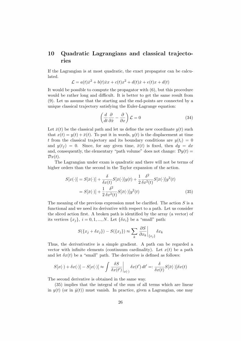
10 Quadratic Lagrangians and classical trajecto-ries

If the Lagrangian is at most quadratic, the exact propagator can be calcu-lated.

L = a(t)x2 + b(t)xx+ c(t)x2 + d(t)x+ e(t)x+ d(t)

It would be possible to compute the propagator with (6), but this procedurewould be rather long and di�cult. It is better to get the same result from(9). Let us assume that the starting and the end-points are connected by aunique classical trajectory satisfying the Euler-Lagrange equation:✓

d

dt

@

@x� @

@x

◆L = 0 (34)

Let x(t) be the classical path and let us define the new coordinate y(t) suchthat x(t) = y(t) + x(t). To put it in words, y(t) is the displacement at timet from the classical trajectory and its boundary conditions are y(ti) = 0and y(tf ) = 0. Since, for any given time, x(t) is fixed, then dy = dxand, consequently, the elementary “path volume” does not change: Dy(t) =Dx(t).

The Lagrangian under exam is quadratic and there will not be terms ofhigher orders than the second in the Taylor expansion of the action.

S[x(·)] = S[x(·)] + �

�x(t)S[x(·)]y(t) + 1

2

�2

�x2(t)S[x(·)]y2(t)

= S[x(·)] + 1

2

�2

�x2(t)S[x(·)]y2(t) (35)

The meaning of the previous expression must be clarified. The action S is afunctional and we need its derivative with respect to a path. Let us considerthe sliced action first. A broken path is identified by the array (a vector) ofits vertices {xj}, i = 0, 1, ..., N . Let {�xi} be a “small” path:

S({xj + �xj})� S({xj}) ⇡Xk

@S

@xk

����{xj}

�xk

Thus, the derivativative is a simple gradient. A path can be regarded avector with infinite elements (continuum cardinality). Let x(t) be a pathand let �x(t) be a “small” path. The derivative is defined as follows:

S[x(·) + �x(·)]� S[x(·)] ⇡Z

�S

�x(t0)

����x(·)

�x(t0) dt0 =:�

�x(t)S[x(·)]�x(t)

The second derivative is obtained in the same way.(35) implies that the integral of the sum of all terms which are linear

in y(t) (or in y(t)) must vanish. In practice, given a Lagrangian, one may

26

collect all terms containing only x and its derivatives, and then calculate Sc

after solving the Euler-Lagrange equation. Then, one gathers all quadraticterms containing only y and its derivatives. The result is:

G(xf , tf ;xi, ti) = exp

i

~Scl(xf , xi)

� Z0

0

Dy(t) exp

i

~

Z tf

ti

dt[ay2 + byy + cy2]

�Consequently, the propagator is the product of a term only depending onthe classical action and a second function F (tf , ti).

G(xf , tf ;xi, ti) = exp [(i/~)Sclassic(xf , xi)]F (tf , ti) (36)

The function F (tf , ti) is the result of a Gaussian integration since the timesliced Lagrangian has only quadratic and linear terms and can be calculatedexactly. It is worth noticing that the propagators under exam only dependon the classical action and trajectory. This is of course a special case, yet,since classical mechanics must be a limit case of the quantum description, itis not unexpected that, under certain conditions, classical quantities appear.The previous result suggests the following approach.

The classic limit can be obtained as ~ ! 0. Then, if ~ is small comparedto S =

RdtL, even small variations of S will result in large variations

of iS/~ in the exponent. Therefore, these rapid phase shifts will producea sort of sum over random numbers on the unitary circumference in thecomplex plane. The mean contribution is expected to be very small. On theother hand, an important contribution should come from those groups ofpaths whose small variations will not a↵ect S significantly. From a classicalpoint of view, such paths must belong to a neighbourhood of the stationarytrajectories for the action-functional, i.e. of those paths satisfying the Euler-Lagrange equation. If the action is expanded in series about the stationarytrajectory and then truncated after the second order (the action will look like(35)), then the approximated propagator can be solved exactly by followingthe foregoing procedure. It can be demonstrated that the semi-classicalpropagator is (in 3 dimensions):

G(xf

, t;xi

) =1

(2⇡i~)3/2

det

✓� @2Sc

@xf@xi

◆� 12

exp

i

~Sc

�(37)

This is called the van Vleck propagator. This approximation is exact forquadratic Hamiltonians. A full description must account for the phase shiftthat occurs any time an eigenvalue of @2Sc

@xf@xichanges sign. Furthermore, if

there are many classical trajectories, G will be a sum of addends like (37).

Let us point out that, despite its appearance, @2Sc@xf@xi

is only a function of

time since both xf and Sc only depend on time once the classical trajectoryis fixed.

27

Finally, let us observe that, if the classical trajectory is unique for everyxi and xf (e.g. the free particle), then (36) implies:

|G(xf , tf ;xi, ti)|2 = |F (tf , ti)|2 (38)

Hence, (11) implies that that if the initial state is a position eigenvalue, say|xii, then it the particle is equally likely to be found anywhere in space ata given instant, since the distribution |G|2 does not depend on position butit only depends on time. This “probability distribution” is not normalized,and not even normalizable. This is not surprising: as a wavefunction is“squeezed” in space, it spreads in momentum space and, consequently, itis more likely to detect the particle farther. |xii is the limit case with aninfinite momentum uncertainty. Nevertheless, this is not troublesome, for|xii is not a legitimate physical state.

11 Uniform electric field

The propagator of a particle in a uniform electric field belongs to the previouscategory with a(t) = m/2 and e(t) = qE. Indeed:

L = T + qEx

Here

F (tf , ti) =

Z0

0

Dy(t) exp

im

2~

Z tf

ti

dty2�

is the free particle path integral with xf = xi = 0 i.e.p

m2i⇡~t .

The classical action can be obtained by integrating the Lagrangian alongthe classical path xcl(t) = xi + v

0

t + (qE/2m)t2, which is a solution of theEuler-Lagrange equation.

Scl =

Z t

0

(m/2)xcl2(t0) + qExcl(t

0)dt0

Scl =(qE)2

3m+ Et2v

0

+mtv2

0

2+ Etx

0

Finally, by inserting the expression of v0

(xf , t;xi) in the previous equationand by combining all the previous results, it is possible to write the propa-gator:

G(xf , t, xi) =

rm

2i⇡~t exp✓i

~

m(xf � xi)2

2t+

qEt(xf + xi)

2� qEt3

24

�◆

28

12 Harmonic Oscillator

Just like the position representation of the propagator for the free particlewas obtained without explicitly performing the sum over paths, the coher-ent states representation for the harmonic oscillator can be evaluated in asimple way. Let us first observe that the harmonic Hamiltonian induces a“phase rotation” on coherent states.

Hh.o. =1

2mp2 +

m!2

2x2 = ~!(a†a+ 1/2)

withHh.o. |ni = (~! + 1/2) |ni

Then (let ~ = 1):

Uh.o. |zi = Uh.o.

Xn

znpn!

|ni = e�i!t2

Xn

znpn!e�i!nt |ni = e�

i!t2��ze�i!t

↵Thus, the propagator is:

G(zf , t; zi) = hzf |G(t) |zii = ei2!t⌦zf |zie�i!t

↵= exp

� |zf |2 + |zi|2

2+ z⇤fzie

�i!t � i!t

2

�One can verify that (33) yields the correct spectrum:

G(zf , E + i⌘; zi) = lim⌘!0

Z 1

0

dt ei(E+i⌘)tG(zf , t; zi)

= lim⌘!0

e�|zf |2+|zi|

2

2

Z 1

0

dt1Xn=0

eiEt(z⇤fzi)

n

n!e�i!tn�i!t/2

= lim⌘!0

e�|zf |2+|zi|

2

2

1Xn=0

(ziz⇤f )n

n!

1

E � !(n� 1/2) + i⌘.

Hence, the eigenvalues are En = !(n+ 1/2).The propagator in the position representation can be obtained by inte-

grating the previous result four times:

G(xf , t;xi) = hxf |G |xii =Z dz2f

⇡

dz2i⇡

hxf |zf i hzf |G |zii hzi|xii

=

Z dz2f⇡

dz2i⇡ zf (xf )

⇤zi(xi)G(zf , t; zi)

Here we will only report the result which will be necessary for studying themagnetic field.

G(xf , t;xi) =

rm!

2⇡i~ sin(!t) exp

im!

2~ sin(!t)((x2

f + x2i ) cos(!t)� 2xixf )

�(39)

29

13 Uniform magnetic field

The classical trajectory of a charged particle in a uniform magnetic field ais cylindrical helix, coaxial to the direction of the field. Similarly, it canbe shown, in the Schrodinger picture, that in quantum mechanics the eigen-states of such a particle can be factorized in those of a free Hamiltonian and abidimensional harmonic oscillator. Here, the corresponding propagator willbe found with the phase space formalism. Since the Lagrangian dependsexplicitly on the vector potential, the gauge must be fixed. If B = |B| isthe norm of the magnetic field, then A can be written as follows (Landau’sgauge):

A =

24 0Bx0

35The phase space Lagrangian is

L = px� 1

2m

hp� e

cA(x)

i2

= px� 1

2m

p2x + p2z +

⇣py � e

cBx⌘2

�The sliced action SN =

RdtL is, according to (24):

Sn =NXj=1

pn(xn � xn�1

)� 1

2m

p2xn + p2zn +

⇣pyn � e

cBxn

⌘2

��The vector potential has been evaluated in xn since in the Hamiltonian for-malism, the magnetic field can be introduced with the following substitutionpn 7! pn � e

cA(xn). The propagator is then:

G(xf , t;xi) = limN!1

Z NYj=1

d3pj

(2⇡~)3N�1Yl=1

d3xl exp

i

~SN

�

The variables yj and zj only appear in SN asPN

j=1

[pyj(yj �yj�1

)+pzj(zj �zj�1

)] =PN�1

j=0

[yj(py,j�py,j+1

)�zj(pz,j�pz,j+1

)]. SinceRdk exp[(i/~)px] =

(2⇡~)�(x), by integrating over all yj and zj variables, the following termappears in the integral:

N�1Yj=0

(2⇡~)2 �(py,j � py,j+1

)�(pz,j � pz,j+1

)

Hence

G(xf , t;xi) =

Zdpzdpy(2⇡~)2

N�1Yj=1

dxj

NYl=1

dpx,l2⇡~ exp

i

~ (Sy,z + Sx)

�

30

with

Sy,z = py(yf � yi) + pz(zf � zi)� tp2z2m

Sx =NXj=1

pxj(xj � xj�1

)� 1

2m

p2xn +

⇣py � e

cBxj

⌘2

��Sx is the phase space Lagrangian of a one-dimensional harmonic oscillatortranslated of x

0

= (c/Be)py from the origin and with frequency ! = Be/mc(Landau frequency). The integration of exp[(i/~)Sx] is then (39):

Gh.o.(xf , t;xi) =

rm!

2⇡~ sin(!t)⇥

⇥exp

i

~m!

2 sin(!t)

⇥((xf � x

0

)2 + (xi � x0

)2) cos(!t)� 2(xf � x0

)(xi � x0

)⇤�

The integration over pz of exp[pz(zf � zi)� t p2z2m ] yields

Gz(zf , t; zi) =

rm

2⇡i~t expi

~m

2

(zf � zi)2

t

�Then, finally:

G(xf , t;xi) =

Zdpy2⇡~ exp [py(yf � yi)]Gh.o.(py)Gz

py is quadratic in the exponent of the integral and, consequently, the previ-ous integral is then a Gaussian one. The terms containing py or, equivalently,x0

can be written and integrated as follows:Zdx

0

exp

"� i

~m! tan

✓!t

2

◆✓x0

� xf � xi2

� yf + yi2 tan(!t

2

)

◆2

#=

s⇡~

im! tan(!t2

)

Consequently, the propagator is:

G(xf , t;xi) =h m

2⇡i~t

i3/2 !t

2 sin !t2

exp

i

~Sc

�exp

i

~B�

Where Sc is

Sc =m

2

(zf � zi)2

t+!

2cot

✓!t

2

◆⇥(xf � xi)

2 + (yf � yi)2

⇤+ !(xiyf � xfyi)

�which is the classical action. The other term, B, is

B =m!

2(xfyf � xiyi)

31

and it is a boundary term which can be eliminated with a gauge transforma-tion. The previous formula has the following form G = N exp[(i/~)Sclassic].This is not surprising, since the Lagrangian, though not one-dimensional, isquadratic and, as a consequence, all the conclusions about classical pathsand the propagator hold.The way to check that Sc is actually the classical action will be sketched. Thegauge does not need to be changed. In addition, since it is already knownthat the motion along the z axis is a free motion, it is enough to evaluatethe action for the motion on the xy plane. The resulting Lagrangian is:

L =m

2x2 +

m

2y2 +

eB

cxy

The equations of motion are the following:

y + !x = 0 x� !y = 0 ) ...x + x = 0

...y + y = 0

The general solution is:

x =1

sin(!(tf � ti))[(xf � x

0

) sin(!(t� ti))� (xa � x0

) sin(!(t� tf ))] + x0

and the analogue for y (x ! y;xi ! yi;xf ! yf ;x0 ! y0

). x0

and y0

aredetermined by the equations of motion:

x0

=1

2[(xf + xi) + (yf � yi) cos(!(tf � ti))]

x0

=1

2[(yf + yi)� (xf � xi) cos(!(tf � ti))]

This is enough to obtain the classical action Sc by integrating the La-grangian.

It is known that the spectrum for a particle in a magnetic field is discreteif the free motion along z is not taken into account. In order to obtain thisdiscrete spectrum, equation (33) can be used. The poles of the transformedpropagator do not depend on the choice of the starting and the end points.Thus, we set (xi, yi) = 0 and r = (xf , yf ).

G(r, t;0) =m!

4⇡i~ sin !t2

exp

im!

4~ r2 cot(!t

2)

�By defining x := m!r2/~ and z := exp(i!t) the propagator can be rewrittenas (we use sin(↵) = (ei↵ � e�i↵)/(2i)):

G(r, t;0) =m!

4⇡~1

1� zexp

xz

z � 1

�exp

� i!t

2

�exp

�m!r2

4~

�

32

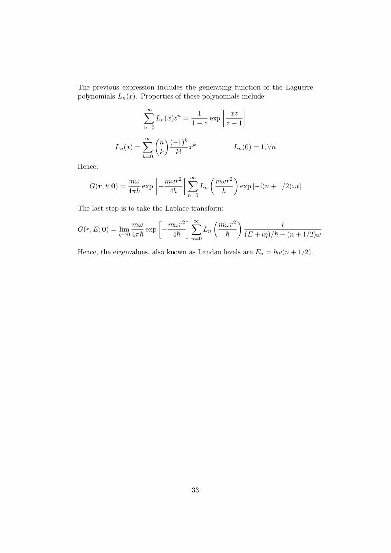
The previous expression includes the generating function of the Laguerrepolynomials Ln(x). Properties of these polynomials include:

1Xn=0

Ln(x)zn =

1

1� zexp

xz

z � 1

�

Ln(x) =1Xk=0

✓n

k

◆(�1)k

k!xk Ln(0) = 1, 8n

Hence:

G(r, t;0) =m!

4⇡~ exp

�m!r2

4~

� 1Xn=0

Ln

✓m!r2

~

◆exp [�i(n+ 1/2)!t]

The last step is to take the Laplace transform:

G(r, E;0) = lim⌘!0

m!

4⇡~ exp

�m!r2

4~

� 1Xn=0

Ln

✓m!r2

~

◆i

(E + i⌘)/~� (n+ 1/2)!

Hence, the eigenvalues, also known as Landau levels are En = ~!(n+ 1/2).

33

Part III

The Aharonov Bohm e↵ect - atopological approach

14 Motivation

The Aharonov-Bohm e↵ect (AB e↵ect from now on) is a well known quantumphenomenon.

Let us consider a charged particle at some point xi and its amplitudeof being, under the quantum dynamics, at some other point xf , where itcan be detected, after a certain amount of time. No force or field is appliedto the particle, so that it can move freely. A solenoid producing a constantmagnetic field is placed somewhere in the experimental set. Two hypothesesare needed: 1) the solenoid is infinitely long and 2) its surface is impenetrablefor the particle. Hence, the magnetic field is confined in an inaccessibleand finite region of space. From the classical point of view, no e↵ect onthe particle trajectory should be observed, since the field has only a locale↵ect (Lorentz force) and it vanishes in the outer region. The quantumcase is di↵erent. In the Schrodinger equation, the quantity accounting forthe electromagnetic interaction is the vector potential and not the Lorentzforce; therefore, a description in terms of vector potential is needed.

There are di↵erent kinds of continuous paths connecting xi and xf andthey can be classified in terms of homotopy classes.

Paths that can be deformed into each other with continuity withoutletting them through the solenoid (and without “cutting” them) belong tothe same homotopy class (see appendix). The need for this classification willbe seen as follows. Let us consider, for example, three di↵erent paths A, Band C as shown in figure (1). These paths cannot be deformed one into theother. Let us first choose the paths A and B. Their amplitudes appearingin the path integral are exp((i/~)(SA + (e/c)

RAA)) and exp((i/~)(SB +

(e/c)RB A)) respectively, with SBand SA being free actions. The di↵erence

in phase is proportional to SB � SA +HA. While SB � SA clearly depends

on the particular paths A and B, the quantityZBAdx�

ZAAdx =

IA,B

Adx =

ZSurface(A,B)

Bds = �

is only determined by the homotopy classes of A and B. This is due tothe Stokes theorem. The only relevant quantity is now manifestly the fluxof the magnetic field. The path C winds clockwise around the solenoid.Thus, if we consider B and C, we will find that the di↵erence in phase isproportional to 2�; As for A and C, it is proportional to � again. Therefore,there is a di↵erence in phase between trajectories from di↵erent classes and

34

Figure 1: Path A, B and C cannot be deformed one into the other

this depends on the di↵erence of numbers of windings around the solenoid.This di↵erence is proportional to integer multiples of �. The foregoingobservations imply that the total propagator should be like:

G ⇡X

windings(n)

eiec~n�

Xe

i~S (40)

The amplitudes of paths sharing the same number (and direction) ofwindings have been summed up, yielding the propagator for a single homo-topy class. Afterwards the class propagators have been summed up withan appropriate phase factor determined by the rule presented above. Obvi-ously, since only relative phases are relevant, the phase of an arbitrary classof trajectories has been set to zero and the other “winding numbers” havebeen fixed accordingly.

The expression (40) di↵ers from the free propagator, meaning that themagnetic field, though confined, has a measureable e↵ect on the particle dy-namics. This can be verified experimentally with a double slit experiment asshown in picture (2). The presence of the solenoid will shift the interferencefigure on the screen.

35

Figure 2: Double slit experiment and the AB apparatus

The foregoing discussion leads to concepts like homotopy classes and“winding numbers”, suggesting a topological approach to the problem. Con-sequently, the following sections will deal with path integrals in multiply-connected spaces. The discussion will be more detailed than technicallyneeded for the AB e↵ect since the topic is interesting by itself and has arange of applications including polymer physics, path integral for spinorsand systems of identical particles.

15 Path Integral on multiply connected spaces

The bidimensional physical space in which the AB e↵ect takes place is clearlysimply connected (R2). Instead, the insertion of an impenetrable solenoidis a mathematical idealization and introduces a “hole” in the plane. Thismeans that the physical space can be approximated by a multiply-connectedspace [27]. The new topology can be used to provide a good description ofthe system but, wherever the formalism will lead, no ambiguity due to themultiple-connectiveness should appear in the final result. The forthcomingideas were proposed and, in large part, developed by Schulman [27] [28].

Let us assume, from now on, that the configuration space is arcwiseconnected. In addition, since the space can be regarded as a di↵erentiablemanifold, it is locally isomorphic to R2 and is required to have every rea-

36

sonable local property of regularity. Thus, the space should be consideredlocally simply connected, locally arcwise connected and semi-locally simplyconnected. These local concepts will not be developed since almost no ex-plicit use will be made of them. The required topology is summarized in theappendix.

The first observation is that the Hamiltonian alone does not provide acomplete dynamics as long as the configuration space is not simply con-nected. This can be seen with the following simple example.

Let us consider quantum mechanics on a segment I = [a, b] in which thepoints a and b are identified. The free Hamiltonian is proportional to ��.Given two functions f(x), g(x) 2 L2(I),Z

Idxf⇤(x)(��g)(x) =

=

ZIdx(��f⇤)(x)g(x)� (g0(b)f(b)� g0(a)f(a))+ (f 0(b)g(b)� f 0(a)g(a)).

(41)

Hence, unless proper boundary conditions are imposed, the free Hamilto-nian is not even symmetric. At a more subtle level, even though f ang gvanish at the boundary, �� is essentially self-adjoint only under appropri-ate boundary conditions. Therefore, it is not surprising that path integralsin a multiply-connected spaces su↵er from an additional ambiguity.

Paths connecting the couple of points xi and xf 2 M can be dividedin homotopy classes, say {↵}. Let us first define the “partial amplitude”G↵(xf , t, xi) for a single class ↵ as the sum over all paths in ↵. If nowthe partial amplitudes are summed up, the old sum over all trajectories isrecovered. The core idea is that, in principle, the partial amplitudes canenter the sum with class-dependent factors c↵.

G(xf , t;xi) =X↵

c↵G↵(xf , t;xi) (42)

All the partial amplitudes (class propagators) satisfy Schrodinger equationindividually. Let us consider the universal covering space M⇤ (it must beassumed that there exists one) and a covering projection p. All paths can belifted via p�1 to M⇤ in a non-ambiguous way according to theorem (3)(seeappendix) once a starting point x⇤i,↵ 2 p�1(xi) is fixed. Let us choose thesame starting point x⇤i for all paths of all classes. On the other hand, if alsothe end-points x⇤f↵ 2 p�1(xf ) were the same for paths in di↵erent classes,these paths could be deformed one into the other (M⇤ is simply connected)and p would map them down in M into the same class (see appendix). Thisis, of course, impossible. In other words, di↵erent homotopy classes in Mare characterized by di↵erent end-points x⇤f↵ in M⇤.

37

Now, let us suppose that everything is well behaved so that the Hamil-tonian, the Schrodinger equation and the Lagrangian can be lifted with p�1

to M⇤. Since M⇤ is simply connected, there is no possible ambiguity whencalculating the propagator G↵ from x⇤i to x⇤f for a given class. Yet, whengoing back to M, there is no dynamical prescription for not summing thepartial amplitudes with nontrivial coe�cients. Then:

GM(xf , t;xi) =X↵

c↵GM↵ (xf , t;xi) =

X↵

c↵GM⇤

(x⇤f↵, t;x⇤i )

The partial propagators are linear independent functions. This willroughly justified. Suppose thatX

�

K�G�(xf , t;xi) = 0.

Thanks to the regularity hypothesis (semi-local simply-connectiveness), therealways exists an open neighbourhood V of xi which is simply connected, andall paths entirely contained in it must belong to the same homotopy class,say ↵. ↵ partial propagator becomes �-like as t ! 0. Other partial ampli-tudes are sums over paths which must, roughly speaking, reach out distantholes outside V : consequently, they give no contribution if t ! 0. Thisyields K↵ = 0. Now let us choose a new class �. xf can be moved back-wards along a representative b of � (� = [b]) until b ⇢ V and xf 2 V . Theprevious argument implies K� = 0 8� 2 C(xi, xf ).

The numbers c↵ must satisfy certain conditions. In particular, c↵ mustbe a commutative representation of the fundamental group ⇡

1

. There are atleast three di↵erent ways to prove this fact according to DeWitt and Laidlaw[22], Dowker [10] and Schulman [28]. Schulman’s is the most intuitive andgoes as follows.

Let us attach a closed path h (⇠ := [h] 2 ⇡1

(xf )) at xf and let us move xfalong it. While xf moves along ⇠ away and then back to the same positionin M , all the points x⇤f,↵ in M⇤ move to new ⇠-dependent locations x⇤f,↵[h].

Rigorously, this means that each path a ([a] = ↵ 2 C(xi, xf )) undergoes thetransformation ↵! ↵[h], which is clearly a 1:1 map of C(xi, xf ) onto itself.While partial amplitudes change, no physical change has been made on Mand the total propagator must equal the old one up to a [h]-dependent phasefactor.X↵

c↵G↵(xf , t;xi) = ei�⇠X↵

c↵G↵⇠(xf , t;xi) =X↵⇠�1

(ei�⇠)(c↵⇠�1)G↵(xf , t;xi)

Linear independence implies exp(i�⇠)c↵[⇠�1]

= c↵. Now one can choose anew path z (⇣ = [z] 2 ⇡

1

(xf )). If the previous procedure is repeated for [h]and [z] in succession and then for [h z] and it is imposed that the results areequal, finally:

�⇠⇣ = �⇠ + �⇣ .

38

This is the expected commutative representation. It can be shown that|c↵| = 18↵. Let a particular c↵ be 1. Then, a small rearrangement yields:

G(xf , t;xi) =X�2⇡1

ei�↵�1�G�(xf , t;xi)

Dowker’s approach, while less intuitive, may be more general. Let usassume that M can be written as M = M⇤/G with G being a properlydiscontinuous group of homeomorphisms (or, even better, a group of isome-tries). In other words, we have identified the points in M⇤ which belong tothe same orbit of some g 2 G, meaning that M = M⇤/ ⇠ with x⇤

1

⇠ x⇤2

ifx⇤2

= g(x⇤1

) for some g 2 G. This identification determines a covering pro-jection p : M⇤ ! M⇤/G = M; x⇤ 7! [x⇤] =: x. Hence, the points in a singleorbit are nothing but the discrete set p�1(x), x 2 M. Let us fix a represen-tative x⇤

0

in M⇤ for each orbit. The set corresponding to a particular choiceof representatives can be called F and it is, of course, not unique.

A multi-valued wavefunction (x) can be defined on M, by associatingwith every x 2 M a di↵erent value for each preimage of x in M⇤. Thesevalues can be regarded as images of a single-valued wavefunction on M⇤ =[x2M p�1(x), say M⇤ :

(x) 7! { M⇤(g(x⇤0

)); 8g 2 G for some given representative x⇤0

2 p�1(x)}

= { M⇤(x⇤0

) 8x⇤0

2 p�1(x)} (43)

If now g is fixed in the first definition of (x) (or, equivalently, a specificpreimage of x is chosen in the second), then is single-valued at a certainx 2 M. This procedure should be repeated for all x 2 M in order to definea domain F in M⇤. Therefore, the single-valued wavefunction on M isidentified as follows: $ M⇤ |

¯F . However, once a point in F is fixed, allthe other points are. This is a direct consequence of the requirement thatboth M⇤ and are continuous, which suggests that F and M should belocally homeomorphic (x

1

! x2

) x⇤1

! x⇤2

), apart from some unimportantissues at the boundarty of F . There are di↵erent possible choices for Fwhich are all “copies” of M in M⇤ and can be mapped one into the otherby elements in G. In particular, by fixing F =: Fe, all other domains areFg = g(Fe), meaning that they are in 1:1 correspondence with elements ofG.

Physics imposes that the domains Fg are equivalent.

M⇤(g(x⇤)) = ei�g M⇤(x⇤) ) ei�g0g = ei(�g+�g0 )

Thus, {ei�g} is an abelian representation of G. The path integral is readily

39

obtained:

M⇤(x⇤f , t) =

ZM⇤

G(x⇤f , t;x⇤i ) M⇤(x⇤i )dx

⇤i

=Xg2G

Z¯Fg⇠=

MG(x⇤f , t; g(x

⇤i )) M⇤(g(x⇤i ))dx

⇤i .

A small rearrangement of the previous result is needed. One ought to extractthe exp(i�g) from the wavefunction and the propagator and remember thatthe conjugate of exp(i�g) is exp(i�g�1)).

M⇤(x⇤f , t) =Xg2G

ei�gZM⇤

G(g�1(x⇤f ), t;x⇤i ) M⇤(x⇤i )dx

⇤i

=Xg02G

e�i�g0

ZM⇤

G(g0(x⇤f ), t;x⇤i ) M⇤(x⇤i )dx

⇤i

The isomorphism between G and ⇡1

is the final step to recover Schulman’sform. Let us remark that the previous discussion implies that the homotopyclasses are in a 1:1 correspondence with elements of G or ⇡

1

.A trivial but important conclusion is that c↵ = 18↵ 2 C(xi, xf ) is always

a legitimate choice since {1} is a commutative representation of any group.

16 Aharonov-Bohm e↵ect on the circle

A possible model for an ideal AB apparatus is the following. The solenoidcan be regarded as an infinitesimally thin cylinder which confines a finiteflux. The solenoid is set in the origin of the xy plane. The appropriatemagnetic field is thus B = ��2(x)z with � being the flux. The correspond-ing vector potential can be derived from an analogy between the presentcase and an infinite wire with a current density J = I�2(x)z generating amagnetic field (Biot-Savart). The correspondence is A $ B, B $ J and� $ I:

A(x) =�

2⇡

�yi+ xj

x2 + y2=

�

2⇡

1

re✓ (44)

The vector potential appears in the Lagrangian as (e/c)Ar. In polar coor-dinates it becomes (e�/c)✓ so that the Lagrangian can be written:

L =m

2(r2 + r2✓2) +

e

c

�

2⇡✓ (45)

From a classical standpoint, the last term, which accounts for the presence ofthe solenoid, is not physical since the Lagrangian is defined up to the totalderivative of a function. The reason is that it only produces a boundaryterm.

40

Now let us consider a quantum system with the same Lagrangian (morecorrectly, the corresponding Hamiltonian should be considered) in a simplyconnected space (one should cut o↵ some part of M or re-interpret the an-gular coordinate to get rid of multiply connectiveness). The addition of themagnetic term to the free Lagrangian as in (45) corresponds to the unitarytransformation (r, ✓) 7! e(e�/c)✓ (r, ✓), which cannot influence observablequantities and, consequently the magnetic term itself can be transformedaway. In other words, the vector potential produces a gauge-dependentboundary term.

If the space is not simply connected, we cannot get rid of the magneticterm. Indeed

R✓dt = ✓f � ✓i + 2⇡n is manifestly dependent on the number

of windings (n) of a specific path and is not an actual boundary term.

Let us now consider the simple case of a particle confined on a circum-ference centred in the origin. The space under exam is SO(2) (or S1) andits covering space is R. The projection map p is defined as

p : ✓ 7! ✓ � 2⇡

✓

2⇡

�.

The square bracket is the integer part function. The fundamental group⇡1

⇠= (Z,+) is the infinite cyclic group generated by one element (+1 or�1). One can consider a single loop either clockwise or counterclocwise. Byattaching together many loops, one gets closed paths with every possiblenumber or windings in both directions. The elements in G are clearly thetranslations of integer multiples of 2⇡, meaning that G = {Tn such that Tn :✓) 7! ✓ + 2n⇡} ⇠= ⇡

1

⇠= (Z,+).The preimages of ✓f are p�1(✓f ) = {✓f (n) = ✓f + 2⇡n with n 2 Z} and

can be obtained one from the others by applying Tn. The points ✓f (n) arethe end-points for lifted paths of di↵erent homotopy classes of SO(2). Then,these classes are indeed identified by these “winding numbers” n.

According to what was said in the previous section, the whole problemwill be lifted in R. For the homotopy class represented by n, the propagatorreads (I = R2m):

Gn(✓f , t; ✓i) = GR(✓f + 2⇡n, t; ✓i)

=

ZD✓(t) exp

i

~

Zdt

✓I

2✓2 +

e�

2⇡c✓

◆�= GR

free(✓f + 2⇡n, t; ✓i) exp

i

~e�

2⇡c(✓f � ✓i + 2⇡n)

�=

rI

2i⇡~t expi

~

✓(✓f � ✓i + 2⇡n)2

t+

e�

2⇡c(✓f � ✓i + 2⇡n)

◆�Since all information has been used (and the propagator must be uniquelydefined) all coe�cients c↵ can be set to 1. Finally, it should be observed

41

that each addend brings the same multiplicative phase exp((e�/c)(✓f � ✓i))which is a genuine boundary term that can be transformed away with aunitary map. The propagator is then:

G(✓f , t; ✓i) =

rm

2i⇡~tXn2Z

exp

i

~e�

cn

�exp

i

~(✓f � ✓i + 2⇡n)2

t

�(46)

The previous derivation is based on the choice of a mathematical modeldescribing the vector potential (and the magnetic field) which yields thecorrect dynamical description and the topological freedom on coe�cients c↵has been disregarded. However, if one looks back at (46), the propagatorappears as the sum of a free partial propagator multiplied by a phase. Thus,it is possible to consider the phases exp

⇥i~e�c 2⇡n

⇤as the topological coef-

ficients a posteriori. In this more topological interpretation, a coe�cient(which in our case has the form ei�n) represents the phase acquired by a freeparticle after winding n times around the singularity.

17 Aharonov-Bohm e↵ect on the plane

If the radial dimension is restored, the configuration space M becomesR2 � {0}. Its universal covering space M⇤ is R ⇥ (0,1] (or it could beR2 itself). The introduction of the radial coordinate does not a↵ect the rel-evant topology, since the multiple-connectiveness is still due to the angularcoordinate in the very same way as before. The fundamental group is thesame as for SO(2), and so the propagator should be formally alike. Clearly,it is best to use polar coordinates. The covering projection is

p : (r, ✓) 7!✓r, ✓ � 2⇡

✓

2⇡

�◆and is particularly appropriate since it is a local isometry. The direct cal-culation of the propagator is rather lengthy, and then we will just give theformula instead and justify it later. Three references for the direct demon-stration are [18] [5] [16].

G(xf , t;xi) =h m

2⇡i~t

iexp

im

2~t(r2

f + r2i )

� 1Xn=�1

exp

ie�

2⇡~c2⇡n�⇥

⇥Z 1

�1d� exp [i�(✓f � ✓i + 2⇡n)] I|�|

✓� imrfri

~t

◆(47)

Functions I�(y) are the modified Bessel functions which are often associatedwith cylindrical coordinates. The first observation is that if e�/2⇡~c isan integer, then any reference to the magnetic field disappears as if � = 0.

42

Therefore, the propagator should be the free propagator in polar coordinates.The fact that winding numbers do not immediately disappear is only due tothe usual coordinate singularity in polar parameterization which should nota↵ect physics. It is possible to eliminate the winding numbers as follows. Byexpanding Dirac’s comb function D(↵) =

P1n=�1 �(n + ↵) on the Fourier

basis (period 1), one gets:

1Xn=�1

e2⇡in↵ =1X

n=�1�(n+ ↵)

We apply this to (47) and we make use of the even parity of the modifiedBessel functions with integer subscript I(z)n = I�n(z):

G(xf , t;xi) =h m

2⇡i~t

iexp

im

2~t(r2

f + r2i )

� 1Xn=�1

ein(✓f�✓i)In

✓� imrfri

~t

◆Let us call Jn(z) the ordinary Bessel functions. The identities

1Xn=�1

ein✓Jn(z) = eiz cos(✓) Jn(iz) = inIn(z)

allow to rewrite the propagator as

G(xf , t;xi) =h m

2⇡i~t

iexp

im

2~t(r2

f + r2i � 2rirf cos(✓i � ✓f ))

�(48)

which is precisely the free propagator and keeps no track of the windings.The ease with which winding numbers have been dismissed as a coordinate-dependent complication, makes us wonder how the multiply connectivenessappears in (47) instead. Had the mathematical model introduced a solenoidwith a finite radius, it would have been obvious, while in (47) such informa-tion is carried by coe�cients exp

⇥i e�2⇡~c2⇡n

⇤and not by the n dependence

of the “free” partial amplitudes (the integral part). If the coe�cients areinterpreted as a consequence of the introduction of the potential (44) andthe c↵ are set to 1, then those points in which the vector potential is notdefined (the origin) must be excluded from the physical configuration space.On the other hand, if one interprets c↵ = exp

⇥i e�2⇡~c2⇡n

⇤, then the sum over

paths is irreparably split into homotopy classes.Keeping the foregoing observation in mind, since to obtain (48) we have

only made use of a chain of identities, all the passages can be read backwardsand one can redundantly introduce winding numbers in the polar propagatorof the free particle. If we trust the topological formalism enough, each termof the sum can be interpreted as a partial amplitude (as seen before, the par-ticle can be thought of as moving freely in M). Then, in order to introducemultiple-connectiveness, it is enough to add the class-dependent coe�cients

43

which must have the form exp(i�n). If now we impose the appropriate phasechange under a 2⇡ rotation, (47) is justified.

Finally, the interference pattern is given by

|G|2 = 1

2

Xj,l

G⇤jGl +GjG

⇤l

In order to evaluate the pattern, it is convenient to assume that rirfm � ~t,so that the asymptotical form of the Bessel function can be used:

I|�|(z) ⇡1p2⇡z

exp

✓z � �2 � 1/4

2z

◆For convergence’s sake, a small imaginary part can be implicitly added tothe mass m 7! m + iµ, and then one can take the limit µ ! 0. After asubstitution and the evaluation of a Gaussian integral, one gets:

G(xf , t;xi) =1X

n=�1

h m

2⇡i~t

iexp

im

2~t(rf � ri)2

�⇥

⇥ exp

ie�

2⇡~c2⇡n+imrfri2~t (✓f � ✓i + 2⇡n)2

�(49)

The most important partial amplitudes are those which involve the straight-est paths. The corresponding winding numbers are n = 0,�1 and they arereferred to those the paths which do not wind at all. Thus, the probabilitybecomes

P (xf , t;xi

) = G⇤0

G�1

+G⇤�1

G0

= 2⇣ m

2⇡~t

⌘2

cos2✓⇡

✓e�

2⇡~c +rfri(✓f � ✓i � ⇡)

~t

◆◆(50)

Then this is the approximate observable quantity for an idealized experi-mental set.

Finally, let us remark that (47) and (50) show a clear 2⇡~c/e flux period-icity. Consequently, all the quantities of the system that depend on � musthave the same periodicity. Thus, it is convenient to define the fundamentalfrequency

�0

=2⇡~ce

(51)

which is very important in experimental observations.

44

18 Experimental evidence

It was 1960, only a year after Aharonov and Bohm had published theirarticle, when Chambers [8] came up with the results of his experiment aboutthe AB e↵ect. The experimental apparatus closely resembles the ideal oneand it will be briefly described, without indulging in technical details.

A source of electrons S produces two coherent beams which are redi-rected towards an observing plane O by an “electrostatic biprism”. Theelectrostatic biprism (efe) (which is actually unnecessary) is composed ofthree elements: f is a positively charged object and the two objects e aretwo earthed metal plates. The electrostatic field which is produced clearlybends the beams in the correct way.

On the plane O the beams meet and an interference pattern appears(4:a). It should be remarked that this picture is in interesting itself as itshows quantum interference at work. If an extended magnetic field is appliedto the region a0, the interference pattern is displaced on the screen but notdeformed (4:b). This is not surprising since in a semiclassical picture thetrajectories are curved by the Lorentz force.

Let us now introduce a localised magnetic field in the region a, instead.This is achieved by inserting a vertical whisker, i.e. a very thin piece ofmagnetized metal (diameter: 1µm, length: 0.5mm), which plays the role ofthe solenoid. In addition, the whisker is placed “in the shadow” of f , sothat the electrons should not meet it on their way.

Let us apply (51) to the present case: it means that consecutive maximaare expected to occur at a “distance” �

0

. The presence of the electric fielddoes not indeed change the topology of the configuration space, while it willchange the dynamics in some way which is not relevant.

The size of the whisker is not constant and it tapers along the z di-rection. Thus d�/dz is not neglectable. If we imagine electrons movingon di↵erent planes, we must conclude that the enclosed magnetic flux varieswith height and that the single interference fringe should change accordinglywithout a displacement of the pattern as a whole. The interference fringesare consequently expected to tilt as it is evident in (4:c).

The main issue - as remarked by Chambers himself and by his colleaguePryce - is that since the flux varies in the whisker, a compensating radial fieldH = (d�/dz)/2⇡r must be produced in the outer region. In a semiclassicalpicture then the two beams move almost horizontally in a radial magneticfield. As a result, the Lorentz force should bend one beam downwards andthe other upwards, thus creating a tilted interference pattern at a rate whichis consistent with the observation. Nevertheless, Chambers pointed out thatif the classical forces explanation was correct, there should be no fringe shiftat all where the size of the whisker is constant.

The attempt to dismiss the AB e↵ect as the result of some hidden forceis still been carried out and will be quoted later.

45

Figure 3: Chambers’ experimental apparatus. From [8]

Figure 4: a) only biprism b) stray field c) magnetized whisker. From [8]

46

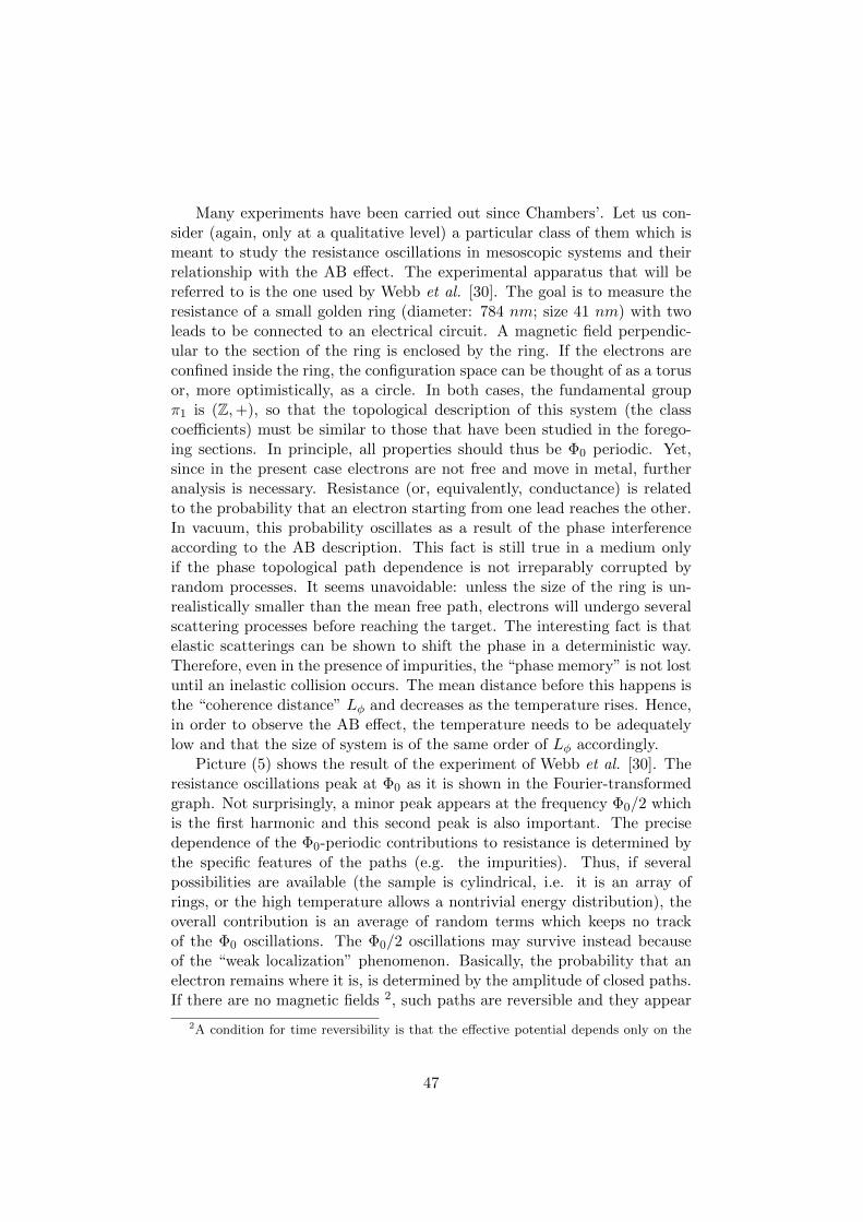
Many experiments have been carried out since Chambers’. Let us con-sider (again, only at a qualitative level) a particular class of them which ismeant to study the resistance oscillations in mesoscopic systems and theirrelationship with the AB e↵ect. The experimental apparatus that will bereferred to is the one used by Webb et al. [30]. The goal is to measure theresistance of a small golden ring (diameter: 784 nm; size 41 nm) with twoleads to be connected to an electrical circuit. A magnetic field perpendic-ular to the section of the ring is enclosed by the ring. If the electrons areconfined inside the ring, the configuration space can be thought of as a torusor, more optimistically, as a circle. In both cases, the fundamental group⇡1

is (Z,+), so that the topological description of this system (the classcoe�cients) must be similar to those that have been studied in the forego-ing sections. In principle, all properties should thus be �

0

periodic. Yet,since in the present case electrons are not free and move in metal, furtheranalysis is necessary. Resistance (or, equivalently, conductance) is relatedto the probability that an electron starting from one lead reaches the other.In vacuum, this probability oscillates as a result of the phase interferenceaccording to the AB description. This fact is still true in a medium onlyif the phase topological path dependence is not irreparably corrupted byrandom processes. It seems unavoidable: unless the size of the ring is un-realistically smaller than the mean free path, electrons will undergo severalscattering processes before reaching the target. The interesting fact is thatelastic scatterings can be shown to shift the phase in a deterministic way.Therefore, even in the presence of impurities, the “phase memory” is not lostuntil an inelastic collision occurs. The mean distance before this happens isthe “coherence distance” L� and decreases as the temperature rises. Hence,in order to observe the AB e↵ect, the temperature needs to be adequatelylow and that the size of system is of the same order of L� accordingly.

Picture (5) shows the result of the experiment of Webb et al. [30]. Theresistance oscillations peak at �

0

as it is shown in the Fourier-transformedgraph. Not surprisingly, a minor peak appears at the frequency �

0

/2 whichis the first harmonic and this second peak is also important. The precisedependence of the �

0

-periodic contributions to resistance is determined bythe specific features of the paths (e.g. the impurities). Thus, if severalpossibilities are available (the sample is cylindrical, i.e. it is an array ofrings, or the high temperature allows a nontrivial energy distribution), theoverall contribution is an average of random terms which keeps no trackof the �

0

oscillations. The �0

/2 oscillations may survive instead becauseof the “weak localization” phenomenon. Basically, the probability that anelectron remains where it is, is determined by the amplitude of closed paths.If there are no magnetic fields 2, such paths are reversible and they appear

2A condition for time reversibility is that the e↵ective potential depends only on the

47

Figure 5: Magnetoresistance at 0,01 K. From [30]

48

in pairs (one the inverse of the other with the same phase) they produceconstructive interference when � = 0 and give a positive contribution toresistance. If the magnetic field is turned on, resistance decreases as thepairs acquire a phase factor. Let us consider those paths that wind once(if they don’t wind they are not influenced by � and, if they wind manytimes, they are too long): since they enclose the flux twice as a pair, thefundamental oscillations acquire a �

0

/2 frequency. Since now the resistancedependence on � is completely determined (e.g. it is maximal at �=0 andmultiple integer of �

0

/2) there is no room for statistics. Two necessaryconditions for the weak localizations to occur are that the magnetic fielddoes not strongly interact with the ring and that L� is long enough.

It must be remarked that these resistance experiments, while interestingon a phenomenological standpoint, give in general little contribution to theunderstanding of the true nature of the AB e↵ect, since the magnetic fieldis not prevented from reaching the ring. Thus, the puzzle of the no-fieldinteraction is not so evident.

It is worth mentioning another two more of experiments whose purposewas to further investigate whether any force is actually involved in the ABe↵ect. The first was similar in purpose to Chambers’. Instead of attemptingto create a long impenetrable solenoid, a toroidal magnet clad with a super-conducting shield was placed between the source of electrons and the targetsurface. The toroidal shape has the advantage of limiting the field leakage.The experiment (Tonomura et al) successfully showed the AB e↵ect as anappropriate displacement of the interference pattern.

In 2007 [7] further evidence was produced against a classical force-basedexplanation of the AB e↵ect. Let us consider the solenoid formulation. Pre-vious theoretical works had hinted that the two beams passing on the leftand on the right could be subject to two opposite forces, one pushing for-ward the electrons and the other pulling them back. Hence, the relativedisplacement of the left and right wave packets could quantitatively accountfor the shift of the interference pattern and no phase shift would be needed.But, if this was the case, there would be a � dependence of the time of flightof the electron which was not observed when a beam was sent through thehole of a square toroidal electromagnet. However, the magnet was macro-scopic whereas the AB e↵ect is usually recorded at a considerably smallerscale. The relevance of the size might be related to the interaction time and,consequently, to the response of the solenoid to the passage of the electrons.

position. It must be remarked that this is a time reversal in a loose sense: it only applies

to the particle motion and not to the whole system. In particular, it does not apply to the

magnetic field. Thus, the trajectory of non-relativistic particle in a fixed magnetic field

is not reversible and, in this case, it can be checked in the path integral formalism that

G(x1, t;x2) 6= G(x2, t;x1).

49

19 Interpretation

In the prevuois section a possible approach to the AB e↵ect has been de-scribed, but there are of course other possibilities. While there seems to begeneral agreement on the result, its interpretation is a pretty subtle matterand is still controversial. Here is an idea of the debate.

It has been originally [1] suggested that either the particle is non-locallyinteracting with the confined magnetic field or that the dynamics of particleis locally influenced by the vector potential alone. Thus, the vector potentialand not the magnetic field would be the fundamental quantity. This seemsto be the commonly accepted explanation, consistent with the fact thatit is the vector potential and not the magnetic field (Lorentz force) whichappears in the Schrodinger equation. However, this may sound troublesomesince the vector potential is only defined up to a gauge transformation.

It is also possible to take seriously the topological approach and re-gard it not just as a good tool. In this case, the fundamental quantityfor the AB e↵ect may be the flux � or even just the topological phaseexp [i(e/c~)�]. Bernido and Inomata [5] argued that the AB e↵ect could beobtained from topological arguments alone since, if it was the case, topolog-ical e↵ects should be observed in simple double slit experiments too. Thesetopological concepts have been refined and they have also been related togauge fields. The topological nature of the AB phase seems to be generallyaccepted too.

Of course much of the interpretation process relies on how much we trustthe approximation, since of course infinitely long solenoids cannot be builtand the magnetic field cannot be completely prevented from “leaking” inthe outer region. But, much more important, the solenoid cannot be trulyimpenetrable and the particle cannot be prevented from tunnelling insidethe solenoid at all or simply from interacting with the solenoid carriers.

It should be remarked that the AB e↵ect does not describe a situation inwhich there is a potential which is not associated to a magnetic field. Morerecent papers (Magni, Valz-Gris) [23] suggested that the AB e↵ect can betreated with ordinary quantum mechanics as a limit case by considering asuccession of Hamiltonians Hn which converge, in a nontrivial way, towardsan HamiltonianH1 describing both a localized magnetic field and an infinitepotential wall confining it into a forbidden region.

Finally, the classical force explanation has still supporters such as Boyer[6]. He claims that the AB e↵ect arises from electrodynamics of pointwiseobjects as a relativistic e↵ect, but he argues that this is not evident since itinvolves little known classical phenomena.

50

A Appendix: minimal homotopy theory

This brief appendix is meant to introduce the terminology and operativedefinitions rather than to explain the subject in a complete and consistentway.Let X be a topological space and I=[0,1]

Definition 1. A path is a continuous map ↵ : I ! XThe set of all paths such that ↵(0) = x

1

and ↵(1) = x2

will be denotedas C(x

1

, x2

). There exists an associative product between paths

⇤ : C(x1

, x2

)⇥ C(x2

, x3

) ! C(x1

, x3

) ⇤ : (a, b) 7! ab

which simply means that if the starting point of b is the end-point of a thetwo paths can be attached to form a new one. The parameter t is rescaledso that ab(0) = x

1

, ab(1/2) = x2

and ab(1) = x3

. Given a path a(t) theinverse path is defined as a�1 := a(�t). A path e is said to be null ife(t) = x 8t 2 I. For any other path a, ae = ea = a whenever the product iswell defined.

Definition 2. X is arcwise connected if C(x, x0) is non-empty 8x, x0 2 XDefinition 3. Two paths a and b 2 C(x

1

, x2

) are said to be homotopic ifthere exists a continuous function

h : I ⇥ I ! X such that h(0, t) = a(t) and h(1, t) = b(t)

Given C(x1

, x2

), homotopy defines an equivalence relationship betweenpaths: a ⇠ b ) [a] = [b]. Homotopy classes will be labelled with greekletters. Let us call ⇡(x

1

, x2

) = C(x1

, x2

)/ ⇠. Given a point x, let us denote⇡1

(x) = ⇡(x, x) the quotient set of all closed paths starting and ending atx.

Homotopy is compatible with the product: composition, associativityand inversion do not depend of the choice of the representative. Therefore,the product can be defined for homotopy classes by using representativeelements [a][b] = [ab].

Theorem 1. Given a point x 2 X , ⇡1

(x) is a group with the multiplica-tion between homotopy classes and it is called the fundamental group atbasepoint x.

If X is arcwise connected, fundamental groups at all basepoints are iso-morphic and can be simply called ⇡

1

. Given x and x0, f : ↵ 2 ⇡1

(x) 7![c�1]↵[c] 2 ⇡(x0) is an isomorphism if c 2 ⇡(x, x0).

Definition 4. X is simply connected if it is arcwise connected and ⇡1

= {e}.

51

Now let X ⇤ be another topological space

Definition 5. Let X be connected. p : X ⇤ ! X is a covering projection

if, 8x 2 X , there exists an open set V ⇢ X such that x 2 V and p�1(V ) =Si Ui. Ui are open and disjoint sets in X ⇤ and the restriction of p to Ui is

a homeomorphism.If X⇤ is connected and simply connected, p is a universal covering.

Not all topological spaces have a universal covering, but, when they do,it is unique up to a homeorphism.

Theorem 2. If p is a covering projection, it is also a local homoemorfism.In addition, #p�1(x) = #p�1(x0)8x, x0 2 X

Now we will use p to lift paths from X to X ⇤

Theorem 3. Let a 2 C(x, x0) be a path in X . The path p�1a : X ! X ⇤ isuniquely defined if p�1a(0) is fixed.

This follows from the fact that p is a local homeomorphism. Once oneof the preimages of a(0) is chosen in one of the Ui (p(Ui) = V which is aneighbourhood of a(0)) then the homeomorphism grants injectivity so thatthe part of the path in V is lifted unambigously. One chooses a new point,say a(t0) 2 V , and fixes a new open set V 0. Since p�1a must be continuous inX⇤ and U 0

is are disjoint, there is only one possible preimage U 0i of V

0 whichcan be chosen. One proceeds this way until a(1) is lifted.

On the other hand, the projection function clearly allows sending pathsfrom X ⇤ to X in a non ambigous way p : C⇤(x⇤i , x

⇤f ) ! C(p(x⇤i ), p(x

⇤f )); a 7!

pa. There is a relationship between omotopy classes in X ⇤ and those in X .Given a, b 2 C⇤(x⇤i , x

⇤f ) if a ⇠ b in X ⇤, then pa ⇠ pb in X . The converse is

not true and this fact is one of the keys to path integral in multiply connectedspaces. If the paths are closed, the following theorem, which clearly appliesto the covering projection, holds.

Theorem 4. Let f : X ⇤ ! X be a continuos map. Then there exist anhomomorphism f : ⇡

1

(x⇤) ! ⇡1

(f(x⇤)) 8x⇤ 2 X ⇤. If f is a homeomorphism,f is an isomorphism.

There is another important object.

Definition 6. Let G be a group of homoeomorfism from X ⇤ to itself. Itsaction on X ⇤ is properly discontinuos if 8x⇤ 2 X has a neighbourhood Usuch that 8g 2 G, g 6= e, g(U) \ U = ;

To our practical purpose, pictorially, elements in G make single points“jump” without dragging them continuously along paths. Then an appro-priate subset (somehow to be called X ) can be chosen and its images underelemnts g cover X ⇤ completely without overlapping. The following theoremdescribes this correctly.

52

Theorem 5. If G acts properly discontinuosly on X ⇤ and X ⇤/G is connected,then p : X ⇤ ! X ⇤/G(=: X ) is a covering projection.

Theorem 6. Let X ⇤ be simply connected and let G acts properly discontin-uosly on it, then X ⇤/G is isomorphic to ⇡

1

.

53

References

[1] Y. Aharonov, D. Bohm, Significance of Electromagnetic Potentials inQuantum Theory, The Physical Review, 115 (1959) 485

[2] Y. Aharonov, D. Rohrlich, Quantum Paradoxes. Quantum Theory forthe Perplexed, Weinheim, Wiley-VCH, 2005

[3] V. Bargmann, P. Butera, L. Giraldello, J. Klauder, textitOn the com-pleteness of coeherent states, Reports on mathematical physics, 2(1971) 221

[4] H. Batelaan, A. Tonomura, The Aharonov-Bohm e↵ects: Variations ona subltle theme, Physics Today, 62 (2009) 38

[5] C.C. Bernido, A. Inomata, Path integrals with a periodic constraint:the Aharonov Bohm e↵ect, Journal of Mathematical physics, 22 (1981)715

[6] T. H. Boyer, Classical Interaction of a Magnet and a Point Charge: TheClassical Electromagnetic Forces Responsible for the Aharonov-BohmPhase Shift, ARXIV (eprint arXiv:1408.3745), 2014

[7] A. Caprez, B. Barwick, H. Batelaan, Macroscopic Test of the Aharonov-Bohm E↵ect, Physical Review Letters, 99 (2007) 210401

[8] R.G. Chambers, Shift of an electron interference pattern by enclosedmagnetic flux, Physical Review Letters, 5 (1960) 3

[9] E. D’Emilio, L.E. Picasso, Problemi di Meccanica Quantistica consoluzioni, Pisa, Edizioni ETS, 2011 [2nd ed.]

[10] J. S. Dowker, Quntum mechanics on multiply connected spaces and onhomogeneous spaces, Journal of General Physics A, 5 (1972) 936

[11] R.P. Feynman, Space-Time Approach to Non-Relativistic Quantum Me-chanics, Reviews of Modern Physics, 20 (1948) 367

[12] R.P. Feynman, A.R. Hibbs, Quantum Mechanics and Path Integrals,New York, McGraw-Hill Book Company, 1965

[13] J. Glimm, A. Ja↵e, Quantum Physics. A Functional Integral Point ofView, New York, Springer-Verlag, 1981

[14] C. Grosche, F. Steiner, Handbook of Feynman Path Integrals, Berlin,Springer-Verlag, 1998

[15] Y. Imry, Introduction to mesoscopic phyisics. Second edition Oxford,Oxford University Press, 2002

54

[16] C. C. Jerry, V. A. Sing, Feynman path integral approach to theAharonov-Bohm e↵ect, Physical Review, 20 (1979) 2550

[17] G. W. Johnson, M. L. Lapidus, The Feynman Integral and Feynman’sOperaltional Calculus, Oxford, Oxford University Press, 2000

[18] D.C. Khandekar, S.V. Lawande, K.V. Bhagwat,Path-Integral Methodsand their Applications, Singapore, World Scientific, 1993

[19] J.R. Klauder, B. Skangerstam, Coherent States, Applications in Physicsand Mathematical Physics, Singapore, World Scientific, 1985

[20] H. Kleinert, Path Integrals in Quantum Mechanics, Statistics, PolymerPhysics and Financial Markets, Singapore, World Scientific, 2004 [3rded.]

[21] T. Kramer, C. Bracher, Propagation in crossed electric and mag-netic fields: The quantum source approach arXiv:cond-mat/0309424 v1(2003)

[22] M. Laidlaw, C.DeWitt, Feynman Functional Integrals for Systems ofIndistinguishable Particles, Physical Review D, 3 (1971) 13765

[23] C. Magni, F Valz-Gris, Can elementary quantum mechanics explain theAharonov-Bohm e↵ect?, Journal of Mathematical Physics, 37 (1995)177

[24] M. Manetti, Topologia. Seconda Edizione, Milano, Springer-Verlagh,2014

[25] F. Oliver et al, NIST Handbook of Mathematical Functions, Cambridge,Cambridge University Press, 2010.

[26] J. Sakurai, Meccanica quantistica moderna. Ristampa ampliata,Bologna, Zanichelli,1996 [1st ed. 1985]

[27] L.S. Schulman, Approximate Topologies, Journal of MathematicalPhysics, 12 (1971) 304

[28] L.S. Schulman, Techniques and Application of Path Integration, Mine-ola, New York, Dover Publications, Inc., 2005 [1st ed. 1981]

[29] S. Washburn, R. Webb, Ahahronv-Bohm e↵ect in normal metal. Quan-tum coherence and transport, Advances in Physics, 35 (1986) 412

[30] R. A. Webb, S. Washburn, C.P. Umbach, R.B. Laibowitz, Observationof h/e Ahahronov-Bohm Oscillations in Normal-Metal Rings, PhysicalReview Letters, 54 (1985) 2696 .

55

[31] J. Zinn-Justin, Paths Integrals in Quantum Mechanics, Oxford, OxfordUniversity Press, 2005

56