Link¶ping Studies in Science and Technology Dissertation No. 1419
172
Linköping Studies in Science and Technology Dissertation No. 1419 Department of Computer and Information Science Linköping University SE-581 83 Linköping, Sweden Linköping 2012
Transcript of Link¶ping Studies in Science and Technology Dissertation No. 1419

Linköping Studies in Science and Technology
Dissertation No. 1419
� � � � � � � � � � � � � � � � � � � � � � � � � � � � � � � � �� � � � � � � � � � � � � � � � � �� � � � ! " # $ % & ' ( ) * + � $ & ' , * - � ( * � %. � � � / � � � � �
Department of Computer and Information Science Linköping University
SE-581 83 Linköping, Sweden
Linköping 2012

ii
Copyright © 2012 Erik Kuiper
Cover designed by Liana Pop
UAV images on cover copyright © Saab AB
ISBN 978-91-7519-981-8
ISSN 0345-7524
Electronic version available at: http://urn.kb.se/resolve?urn=urn:nbn:se:liu:diva-72792
Printed by LiU-Tryck 2012

iii
� � � � � � �Communication is a key enabler for cooperation. Thus to support efficient communication humanity has continuously strived to improve the communication infrastructure. This infrastructure has evolved from heralds and ridden couriers to a digital telecommunication infrastructures based on electrical wires, optical fibers and radio links. While the telecommunication infrastructure efficiently transports information all over the world, there are situations when it is not available or operational. In many military operations, and disaster areas, one cannot rely on the telecommunication infrastructure to support communication since it is either broken, or does not exist. To provide communication capability in its absence, ad hoc networking technology can be used to provide a dynamic peer-based communication mechanism. In this thesis we study geographic routing in intermittently connected mobile ad hoc networks (IC-MANETs).
For routing in IC-MANETs we have developed a beacon-less delay-tolerant geographic routing protocol named LAROD (location aware routing for delay-tolerant networks) and the delay-tolerant location service LoDiS (location dissemination service). To be able to evaluate these protocols in a realistic environment we have used a military reconnaissance mission where unmanned aerial vehicles employ distributed coordination of their monitoring using pheromones. To be able to predict routing performance more efficiently than by the use of simulation, we have developed a mathematical framework that efficiently can predict the routing performance of LAROD-LoDiS. This framework, the forward-wait framework, provides a relationship between delivery probability, distance, and delivery time. Provided with scenario specific data the forward-wait framework can predict the expected scenario packet delivery ratio.
LAROD-LoDiS has been evaluated in the network simulator ns-2 against Spray and Wait, a leading delay-tolerant routing protocol, and shown to have a competitive edge, both in terms of delivery ratio and overhead. Our evaluations also confirm that the routing performance is heavily influenced by the mobility pattern. This fact stresses the need for representative mobility models when routing protocols are evaluated.
This work has been supported by LinkLab, a research center for future aviation
systems, established by Saab and Linköping University, and the KK foundation
through the industrial graduate school SAVE-IT.

iv

v
� � � � 0 1 � � � � � 2 � � � � � � � � � � �� 3 � � � � � � � � 3 � � �4 5 6 7 6 8 9 : ; < = > = 5 ? @ A 6 9 B C B 5 > ; 7 D 8 @ > B 7 5 > B 9 9 A < E A 5 D 9 B 5 C = 5Idag förväntar vi oss att vi kan komma ut på Internet nästan var som helst och omedelbart få kontakt med vänner och bekanta. Skälet att denna möjlighet finns är att vi har byggt upp en omfattande infrastruktur som hjälper oss att skicka datapaket fram och tillbaka. Låt oss anta att denna infrastruktur inte längre finns och att det enda som finns tillgängligt är de elektroniska apparater vi bär på oss med trådlösa anslutningsmöjligheter som Wi-Fi. Genom att samarbeta och skapa ett ad hoc-nätverk med hjälp av dessa apparater är det möjligt, men långt från trivialt, att skicka information mellan personer som inte kan kommunicera direkt med varandra.
I ett ad hoc-nätverk ansvarar ett routing-protokoll för att hitta en väg i nätverket för datapaket så de kommer fram till rätt mottagare. Routing-protokollet skickar ett paket trådlöst från apparat till apparat tills det kommer fram till mottagaren. Det har dock visat sig svårt att designa routing-protokoll som fungerar bra då de personer som bär på apparaterna rör på sig. Ett annat problem är att det ibland inte finns någon väg för ett paket att nå mottagaren. Skälet är oftast att det saknas personer på strategiska platser som gör att nätverket delas upp i öar där snabb kommunikation bara fungerar inom dessa öar. Man säger då att nätverket är partitionerat. Om vi däremot kan tänka oss att vara lite tålmodiga så kan vi tillåta att tillfälligt lagra vårt paket hos en person som kommer att röra på sig och komma till ”ön” där mottagaren finns. När detta sker så kan paketet levereras, dock med en större fördröjning. Den fördröjning vi pratar om här är lite för lång för att fungera med ett chatt-program, men för e-post fungerar det bra.
Ett sätt att göra jobbet enklare för routingprotokollet är om vi kan skicka paketet till den geografiska position där mottagaren befinner sig. Detta kräver att alla elektroniska apparater vet var de befinner sig, men med GPS-mottagare i nästan varje apparat är detta oftast inget hinder. För att veta var mottagaren befinner sig behöver routingprotokollet ta hjälp av en lokalisationstjänst som kan förmedla denna information.

vi
Vi har tagit fram ett routingptotokoll, LAROD, för geografisk routing i system med mobila noder där mobiliteten måste utnyttjas för att leverera paketen då systemet är partitionerat. För att kunna leverera information om var en mottagare befinner sig har vi tagit fram en lokaliseringstjänst, LoDiS. Då vi inte tror att det främst är du och jag som har behov av denna typ av routing (vi har ju tillgång till en infrastruktur), så har vi utvärderat dessa protokoll i ett militärt spaningsscenario. I spaningsscenariot har vi antagit att ett antal obemannade flygfarkoster (UAVer) samarbetar för att spana av ett visst område. När en UAV upptäcker något av intresse rapporterar den denna information till en annan UAV som kan agera på informationen. I våra utvärderingar av protokollen har vi sett att de fungerar väl och att informationen kommer dit den skall (även om det tar lite tid).

vii
� � � � � � � � � � � � �First I want to thank Saab Aeronautics, and then especially Anders Pettersson and Gunnar Holmberg, for giving me this opportunity to pursue a PhD. Without the connection to a practically applicable problem domain I would probably not have chosen doctoral studies. Tomas Jansson, my manager when this journey started, was also important since he helped me find this challenge when I needed it. I also want to thank my industrial advisor Mats Ekman. I might not have sought your advice that extensively, but the discussions we had gave me some things to think about. I also owe gratitude to Magnus Svensson and Anders Bodin, my project leader and manager respectively, for accepting that I could not spend all my time on the project I was part of at Saab.
To my academic advisor and supervisor Simin Nadjm-Tehrani I would like to extend a thank for guiding me to this point. You especially taught me how to write for an academic audience and not only to report my findings. I might not entirely agree with the anatomy of academic articles, but hopefully I now understand it reasonably well. To Di Yuan, my assisting academic advisor, I give my thanks for helping me with the formal definition of the forward-wait framework.
I also want to thank the other members of RTSlab for your friendship and valuable comments. You helped me to become aware of some of the assumptions I hade made and you pushed me to clarify and further investigate some issues.
I am grateful to SAVE-IT and the KK foundation for partially funding my research. You might not be in my thoughts every day, but without you this research might never have been done.
Finally I want to thank my friend C. Without you I might never have selected to work for Saab, and then this would never have happened.
Erik Kuiper
Linköping, January 2012

viii

ix
F � � � � �1 Introduction ............................................................................................... 1
1.1 IC-MANETs............................................................................................ 31.2 Node Mobility ........................................................................................ 41.3 Problem Description.............................................................................. 51.4 Contributions ......................................................................................... 61.5 Thesis Outline......................................................................................... 9
2 Related Work ........................................................................................... 11
2.1 Routing ................................................................................................. 112.1.1 Delay-tolerant Routing............................................................... 132.1.2 Geographic Delay-tolerant Routing .......................................... 152.1.3 Opportunistic Routing................................................................ 172.1.4 Beacons-less Routing .................................................................. 18
2.2 Location Services ................................................................................. 202.3 Routing Modeling ................................................................................ 23
2.3.1 The ICT Model ............................................................................ 252.3.2 Other Routing Models................................................................ 26
2.4 Mobility Models................................................................................... 272.4.1 Real-World Mobility Models ..................................................... 282.4.2 Synthetic Mobility Models ......................................................... 31
2.5 Node Density and Connectivity ......................................................... 37
3 Reconnaissance Mobility ....................................................................... 41
3.1 Scenario................................................................................................. 413.2 The Three Way Random Mobility Model .......................................... 433.3 The Pheromone Reconnaissance Mobility Model ............................. 433.4 Evaluation............................................................................................. 48
3.4.1 Scan Coverage............................................................................. 503.4.2 Scan Characteristic...................................................................... 543.4.3 Communication potential........................................................... 56
4 Routing in IC-MANETs.......................................................................... 59
4.1 LAROD ................................................................................................. 594.2 LoDiS .................................................................................................... 66
4.2.1 The LoDiS Protocol..................................................................... 674.2.2 The Requirements on Clock Synchronization .......................... 69
4.3 Evaluation............................................................................................. 704.3.1 Scenario Parameters and Set Up................................................ 704.3.2 LAROD Parameters.................................................................... 724.3.3 LoDiS Parameters and Performance ......................................... 73

x
4.3.4 The Impact of the Mobility Model............................................. 754.3.5 LAROD-LoDiS Compared to Spray and Wait ......................... 77
4.4 Concluding Remarks ........................................................................... 82
5 A Framework for Performance Analysis .............................................. 83
5.1 The Forward-Wait Framework........................................................... 835.2 Characterizing Forwarding and Waiting........................................... 89
5.2.1 Abstract Mobility and Routing Model ...................................... 905.2.2 Framework Inputs Based on Models ........................................ 925.2.3 Distributions from ns-2 Data ..................................................... 98
5.3 Characterizing Distance to Destination ............................................1025.4 Validation of the Framework.............................................................103
5.4.1 Delivery Ratio Predictions ........................................................1045.4.2 Distance and Time Predictions .................................................105
5.5 The Validity of the Framework Assumptions ..................................1075.6 Practical Application of the Framework ...........................................109
5.6.1 Delivery Ratio Predictions ........................................................1095.6.2 Source Node Parameter Adjustment .......................................111
5.7 Concluding remarks ...........................................................................113
6 Where We are and Where We Can Go.................................................115
6.1 Summary and Conclusions ................................................................1156.2 Future Work ........................................................................................117
7 Acronyms.................................................................................................119
8 References ...............................................................................................121
Appendix 1 Percolation Theory Metrics ................................................ 133
Appendix 2 Implementing Spray and Wait in ns-2.............................. 135
Appendix 3 Complexity of Deriving the Distribution of Forwarding
Distance ................................................................................ 141
Appendix 4 Random Variables ............................................................... 143
Appendix 5 Distance Distributions Between Pairs of Nodes ............. 145

xi
G � � � � 3 H � � � � � �Figure 1. Network type related to node density........................................... 2Figure 2. OR forwarding example ................................................................17Figure 3. Forwarding areas. ..........................................................................19Figure 4. A taxonomy of location services ...................................................21Figure 5. Change of average direction near the edges. ...............................34Figure 6. UAV line scanning. ........................................................................35Figure 7. Three way random state diagram.................................................43Figure 8. Local pheromone map after 3600 simulated seconds. ................45Figure 9. Global pheromone view after 3600 simulated seconds...............45Figure 10. Local pheromone map after 7200 simulated seconds. ................46Figure 11. Global pheromone view after 7200 simulated seconds...............46Figure 12. Pheromone search pattern.............................................................47Figure 13. Coverage for pheromone mobility with different transfer
probabilities. ...................................................................................51Figure 14. Coverage comparison for pheromone mobility with global map.
.........................................................................................................51Figure 15. Coverage for pheromone mobility with different coverage
factors..............................................................................................52Figure 16. Coverage for different mobility models. ......................................53Figure 17. Pheromone mobility. Coverage variability. .................................53Figure 18. Next scan pdf for different mobility models................................55Figure 19. Next scan pdf for pheromone mobility with different node
degrees. ...........................................................................................55Figure 20. Average number of clusters. Pheromone mobility with different
node degrees...................................................................................57Figure 21. Pheromone mobility. Cluster variability. .....................................58Figure 22. Comparison of different mobility models....................................58Figure 23. Forwarding area examples ............................................................61Figure 24. Delay curve examples....................................................................62Figure 25. Delay time parameters illustration ...............................................63Figure 26. LAROD pseudo code. ....................................................................65Figure 27. LAROD-LoDiS path visualization example. ................................66Figure 28. LoDiS pseudo code. .......................................................................69Figure 29. Delivery ratio with parameterized LoDiS and Pheromone
mobility. ..........................................................................................73Figure 30. Overhead with parameterized LoDiS and Pheromone mobility.74

xii
Figure 31. Average direction error at source node. ......................................75Figure 32. LADOD-LoDiS delivery ratio for different scenarios. ................76Figure 33. LADOD-LoDiS overhead for different scenarios. .......................76Figure 34. Spray and Wait delivery ratio for different scenarios.................77Figure 35. Spray and Wait overhead for different scenarios........................77Figure 36. Delivery ratio for different packet life times under pheromone
mobility. ..........................................................................................78Figure 37. Overhead for different packet life times under pheromone
mobility. ..........................................................................................79Figure 38. Delivery ratio for different transmission loads under pheromone
mobility. ..........................................................................................80Figure 39. Overhead for different transmission loads under pheromone
mobility. ..........................................................................................80Figure 40. Delivery ratio for different node densities under pheromone
mobility. ..........................................................................................81Figure 41. Overhead for different node densities under pheromone
mobility. ..........................................................................................82Figure 42. Time-distance forward illustration. ..............................................84Figure 43. An illustration of minimum progress forwarding area ..............91Figure 44. Probability of being forwarded by at least a given distance from
the source with no initial wait (ccdf), for four node density values. .............................................................................................93
Figure 45. Probability of being forwarded by at least a given distance from the source after a wait (ccdf), for four node density values. ......95
Figure 46. Probability of waiting for at most a given time, for four node density values. ................................................................................98
Figure 47. Probability of being forwarded by at least a given distance from the source with no initial wait (ccdf). .........................................100
Figure 48. Probability of being forwarded by at least a given distance after an initial wait (ccdf). ....................................................................100
Figure 49. Probability of waiting for at most a given time before forwarding (cdf). ..............................................................................................101
Figure 50. Cdf of source-destination distance. ............................................103Figure 51. Predicted and simulated delivery ratio for different TTLs.......105Figure 52. Probability of reaching at least 4 radio radii with respect to time.
.......................................................................................................106Figure 53. Probability of requiring at least 200 seconds with respect to
distance. ........................................................................................107

xiii
Figure 54. Delivery ratio for different sizes of the any-to-any scenario with a constant average node degree. .................................................109
Figure 55. Delivery ratio for different sizes of the any-to-C&C scenario with a constant average node degree. .................................................110
Figure 56. Delivery ratio for different node densities of the any-to-any scenario with a constant area size...............................................111
Figure 57. Delivery ratio for different node densities of the any-to-C&C scenario with a constant area size...............................................111
Figure 58. TLL required for achieving 95% delivery guarantee for various density levels. ...............................................................................112
Figure 59. Delivery probability in distance and TTL. .................................112Figure 60. Packet exchange ...........................................................................136Figure 61. An illustration of the custodian location after first hop............141

xiv

xv
G � � � � 3 I � � � � �Table 1. Random waypoint parameters......................................................32Table 2. Gauss-Markov parameters. ...........................................................33Table 3. Connectivity properties .................................................................39Table 4. Average node degree in different routing studies. .....................40Table 5. Scenario parameters.......................................................................42Table 6. Pheromone map parameters. ........................................................44Table 7. Pheromone parameter definition. .................................................47Table 8. UAV pheromone action table........................................................48Table 9. Never scanned area........................................................................56Table 10. LAROD parameters .......................................................................63Table 11. Basic simulation parameters .........................................................71Table 12. Delivery ratio for different LAROD parameters. ........................72Table 13. Overhead for different LAROD parameters (transmissions per
data packet). ...................................................................................72Table 14. Key notation and terms .................................................................85Table 15. Terms in custodian selection. ........................................................91Table 16. Probability of having an initially empty forwarding area ..........93Table 17. Average probability of forwarding after a retry interval............96Table 18. Notation and terms in deriving distributions for the waiting
phase. ..............................................................................................97Table 19. Average wait times and forward distances. ..............................108Table 20. Percolation theory and ad hoc network parameters, and their
relationships. ................................................................................133Table 21. Spray and Wait implementation choices and rationale. ...........136Table 22. Impact of lost packets on Spray and Wait..................................138Table 23. Scenario parameters.....................................................................139Table 24. Spray and Wait parameters.........................................................139

xvi

1
1 Introduction The sharing of information is vital for many tasks, and the faster information can be disseminated the sooner or better a task can be completed. With the prevalence of wireless technologies like GSM, 3G and Wi-Fi, information is often available anytime and anywhere. The limitation of these technologies is that they require an infrastructure of base stations or access points to function. In environments such as disaster areas, or in certain war zones, this type of infrastructure is generally not available, but information exchange is still desired. In these environments you commonly use long range radios that enable point-to-point communication. The problems with these systems are that they are often expensive, bulky and only provide low bandwidth communication.
At the other end of the spectrum there are cheap, small, low power, high bandwidth, but short range radio technologies. If a lot of actors are equipped with this type of radios then they could automatically form a network and cooperate to forward messages for each other. These types of networks that are cooperatively formed and do not rely on any infrastructure are often called ad hoc networks. To create local ad hoc networks there exist technologies like Bluetooth [93] and ZigBee [112], but the creation of larger and highly dynamic ad hoc networks is still in the research domain.
The study of routing in dynamic and infrastructure-free networks started in the field of mobile ad hoc networks (MANETs). A key assumption made in MANET routing is that any two nodes can always find a connected path to reach each other. Many MANET studies found that this assumption was not always valid and that a significant number of packets were lost in the network due to network partitions. About the same time other researchers were studying how information could be transferred in interplanetary networks (IPN) [39]. In these networks some of the communication links are only available during certain periods and in many cases a contemporaneous end-to-end path is never available. To cope with this they developed the concept of custodians where the responsibility of a data packet is transferred

2 CHAPTER 1
between custodians. The problems addressed by the IPN research were also found in other challenged networks and the field of delay-tolerant networks (DTNs) was defined. The main characteristic of a DTN is that it generally takes a long time for information to reach its intended destination. The reasons for the delays may be long transfer latencies or infrequent communication contacts. This means such disparate networks as IPNs, wildlife tracking systems [52][90] and networking in rural communities [22][76] are all DTNs. In DTN routing research it is common to study systems where the nodes most of the time have no contact with other nodes, and where they only occasionally meet [94]. We call this type of DTN a solitary DTN.
In this thesis we study networks that lie in the region between solitary DTNs and MANETS. We call this type of network intermittently connected MANET (IC-MANET). The characteristic of this network type is that nodes form connected clusters, within which MANET style routing is possible. To reach nodes that are located outside a cluster, DTN style routing is required. Due to the node mobility, the nodes that are part of a cluster constantly change. Figure 1 provides an illustration of how the node density affects the network type. This is a very simplified picture and it assumes that connectivity is improved with increased node density. Due to node aggregation at popular locations a network might never be fully connected, even if the average node density is very high.
Figure 1. Network type related to node density.
The communication performance in an IC-MANET is greatly affected by how the nodes move, which in turn determines the communication opportunities that exist in the system. For this reason it is important to use a relevant scenario when a routing protocol is evaluated. The main evaluation scenario in this thesis is a military reconnaissance mission where a group of unmanned aerial vehicles (UAVs) cooperate to fulfill the reconnaissance requirement. We have also used synthetic random mobility models as comparative references.
Density
Solitary DTN IC-MANET MANET

INTRODUCTION 3
J K J L M N - � O P Q %
MANET research studies how to route data packets in a network of mobile nodes with wireless radios. A key assumption made by all MANET routing protocols is that there exists a contemporaneous end-to-end multi-hop path between any sender and receiver, and when such a path does not exist, they will fail to deliver messages. This does not mean that it is impossible to route messages in the absence of contemporaneous paths, only that other principles need to be used.
In an IC-MANET the system is so sparse, or the nodes are moving in such a way, that there exists at least two clusters of nodes for which there is no contemporaneous path between the nodes in different clusters. Due to node mobility these clusters are not stable, but instead they constantly split and merge. To enable communication between nodes in different clusters messages alternate between multi-hop forwarding within a cluster, and storage until the clusters reform, and further forwarding becomes possible. A consequence of the relatively slower forwarding by node mobility compared to wireless forwards is that delivery times will be longer than if a contemporaneous end-to-end path existed.
In most networks the responsibility for reliable transfer is placed on the source-destination pair, and network failures result in time-outs and resending of data from the source. In a DTN or an IC-MANET this end-to-end reliability mechanism is not a suitable design choice since it relies on status exchanges between the source and destination, exchanges that take significant time in these environments. Instead, the network should guarantee that a message is reliably transferred to the destination. In DTNs this is normally done by transferring the messages between custodians where the custodians guarantee that messages are reliably moved between custodians until the destination is reached. Depending on the system either some or all of the nodes can act as custodians.
When a packet is transmitted from the source the network might not know, and might not be able to determine, where the destination is located due to the disconnected nature of the system. The most straightforward method to send a packet to a node whose location is unknown, and where the best path to reach it is unknown, is to send it to all nodes in the network. This is done by Epidemic Routing [102]. The problem with this method is that it requires significant bandwidth and storage resources. The other extreme is to keep

4 CHAPTER 1
the packet in the source node until the source node meets the destination node due to mobility as is done by Direct Transmission (no relaying) [94]. To be able to better guide a packet to the destination several routing protocols have been proposed that use historical encounter data to decide how to forward a packet. Examples are PRoPHET (v2) [31], SimBetTS [20], and BUBBLE [45].
Another alternative is to send a packet towards the position of the destination. This requires that all nodes are position-aware and that there exists a location service that can provide the position of the destination to the source. Two examples of protocols that perform geographical routing in intermittently connected MANETs are GeoSpray [91] and GeoDTN+Nav [16]. Neither of these two protocols provide any details on a suitable location service for IC-MANETs. Since the nodes in our scenario are location-aware, we have chosen to study the feasibility of geographic routing with a location service in IC-MANETs. J K R
O � ( * - � S ! � ! " T
A key element affecting the performance of MANET and IC-MANET routing is how nodes move. Several MANET studies have shown that the node mobility affects the routing results [47][63][68][82][111]. A property we also have found to be true in the IC-MANETs we have studied. This means that a routing protocol should be evaluated in an environment that as close as possible resembles the environment it will be deployed in. If a routing protocol is intended for general use then it should be tested in several reasonable, but characteristically different, environments.
Most routing protocols have been evaluated using abstract mobility models such as the random waypoint mobility model [50] or the random direction mobility model [84]. This class of mobility models has the benefit of a relatively simple description of the mobility logic. Additionally, some of the mobility models have attractive node distribution properties. The problem is of course that they are not particularly realistic.
A method that can be used to obtain realistic mobility patterns is to use traces from actual node movements. The problem with real-world traces is that they are costly and difficult to obtain, and that many traces are required to achieve good statistical confidence in the evaluation of a routing protocol. Another limitation of real-world traces is that they are unable to provide

INTRODUCTION 5
information on new types of mobility patterns. A practically more attractive option is to use a synthetic mobility model that models a real scenario. A synthetic mobility model can generate as many mobility traces as is required for the evaluations. Examples are the Dispatched Ambulance model by Schwamborn et al. [89], the traffic simulator TRANSIMS provided by the travel model improvement program [101], and trace based campus model by Kim et al. [56]. In this thesis we will mainly study a mobility model that describes the movement of UAVs in a reconnaissance mission. J K U
) � S � * $ V * % , ! W " ! � '
At the time of writing several aerospace companies and universities are working on developing autonomous aerial vehicles. While they currently concentrate on autonomous control of a single or at most a few aircraft at a time, it is expected that the concept of swarming UAVs will be addressed in the future when autonomous control of a single UAV is solved. In the Unmanned Aircraft Systems Flight Plan 2009-2047 for the US Air Force [23] they envision swarming UAVs communicating with MANET technology.
In this thesis we address some of the communication needs in a system of swarming UAVs. While our proposed routing algorithm can be used in other environments, it is the requirements of swarming UAVs that drives the design. As the main evaluation scenario we have chosen a reconnaissance mission in which a group of UAVs shall detect units on the ground by regularly scanning all parts of a specified area. Since it is probable that the units on the ground do not want to be detected by the UAVs there ought to be no apparent pattern to when a UAV scans a particular area. The same type of requirements can be found on the searching behavior in the FOPEN (Foliage Penetration) scenario reported in the work by Parunak et al. [74]. Since most mobility models used in MANET research are either synthetic [11] or based on human mobility [44][56][82][99] we have had to develop a mobility model for this scenario.
Under a reasonable selection of node density and communication range the nodes moving under our mobility model will form an intermittently connected network. The challenge is then to route messages in a reliable manner while observing system resource limits, such as storage, power and wireless bandwidth, in the realistic mobility scenarios envisioned. Since UAVs are location-aware due to navigational requirements the positional knowledge can be used to perform geographic routing. For geographic

6 CHAPTER 1
routing to work two elements are required, a routing protocol that routes a packet to the destination’s position, and a location service that keeps track of where the destination is. For the routing protocol we will explore the viability of beacon-less geographic routing. Beacons are regularly transmitted special messages that are used by many routing algorithms to determine a node’s neighbors. The reason to evaluate beacon-less routing is that beacons, as commonly used by routing protocols, have the following problems [36]:
• They consume a lot of bandwidth.
• The consume energy from nodes even if they are not performing any routing.
• Beacon information may not accurately represent actual communication possibilities due to node mobility after beacon reception and due to fading.
For the location service we need to find a system that can cope with the network disconnections and the limits this brings with regard to information spreading and the limited availability of low latency communication to other nodes. J K X
M � ' " ! S Y " ! � ' %The main contributions in this thesis are as follows.
• A mobility model with distributed control for area reconnaissance applications.
• A novel geographic routing algorithm for IC-MANETs.
• A distributed location service for IC-MANETs.
• A mathematical framework that efficiently estimates the routing performance of geographic routing algorithms in IC-MANETs.
A distributed pheromone mobility model for reconnaissance applications
To evaluate our proposed routing protocol we have used a military reconnaissance scenario. The objective in the scenario is for a group of UAVs to cooperatively and regularly scan an area to detect units on the ground. Since it is probable that the units on the ground do not want to be detected the UAVs should not move in a deterministic pattern.

INTRODUCTION 7
To coordinate the UAVs we have designed a swarming inspired mobility model based on distributed pheromones. By using pheromones and localized search the UAVs are guided to areas not recently visited by other UAVs. When a UAV moves around it places pheromones on the areas it has scanned. Since it is not possible to place these pheromones in the environment, as it would be done in a natural system, the UAV places them in a local pheromone map. To share this pheromone information with the other UAVs each UAV regularly broadcasts a local area pheromone map. All UAVs that receive the broadcast merge this information into their own pheromone map.
The distributed pheromone mobility results presented in this thesis extends the results presented in the following paper:
Erik Kuiper, Simin Nadjm-Tehrani. Mobility Models for UAV Group
Reconnaissance Applications. Proceedings of International Conference on Wireless
and Mobile Communications. July 2006. IEEE
A beacon-less geographic routing protocol for intermittently connected
networks
Most MANET and IC-MANET routing protocols use beacons to know who their neighbors are. While it is a quite simple and effective method, it has the problem of creating significant overhead. Additionally, the information gathered by beacons is always out of date to some extent.
In this thesis we present location-aware routing for delay-tolerant networks (LAROD). LAROD forwards messages using greedy geographic routing without the use of beacons and employs the store-carry-forward principle when a message cannot be forwarded due to network partitions.
LAROD was originally presented in:
Erik Kuiper, Simin Nadjm-Tehrani, Geographical Routing in Intermittently
Connected Ad Hoc Networks. The First IEEE International Workshop on
Opportunistic Networking. March 2008. IEEE
A location service for intermittently connected networks
While there exists some other proposals regarding geographic routing in IC-MANETs, we have not found any proposed location services. The problems with a location service in an IC-MANET are twofold. First, there is an issue with the fact that large parts of the system cannot get up-to-date information due to network partitioning. Secondly, one needs to deal with the fact that,

8 CHAPTER 1
in the worst case, a source node is isolated in a cluster that only consists of the node itself.
In this thesis we present the Location Dissemination Service (LoDiS). In LoDiS all nodes act as location servers and the location data is updated by data exchanges as nodes encounter each other.
LoDiS is presented with an integrated version of LAROD in the following paper where the complete routing system is evaluated:
Erik Kuiper, Simin Nadjm-Tehrani. Geographical Routing With Location Service in
Intermittently Connected MANETs. IEEE Transactions on Vehicular Technology.
Volume 60, Number 2, February 2011. IEEE
A mathematical framework for geographic routing in IC-MANETs
Simulation is a useful, but time consuming, tool to estimate routing performance. Moreover, packet level simulators with physical layer implementations close to reality, such as ns-2, commonly limit the network size to a couple of hundred nodes. To be able to determine the routing performance more efficiently in a new or large scenario a mathematical framework can be very useful.
In this thesis we present a general mathematical framework, the forward-wait framework, for the analysis of geographic routing protocols in IC-MANETs. Within the framework the movement of a packet is characterized by a sequence of alternating forwarding and waiting phases.
The mathematical model of geographic routing in IC-MANETs is previously presented in:
Erik Kuiper, Simin Nadjm-Tehrani. Predicting the Performance of Geographic
Delay-Tolerant Routing. Military Communications Conference (MILCOM). 2011.
IEEE
Erik Kuiper, Simin Nadjm-Tehrani, Di Yuan. A Framework for Performance
Analysis of Geographic Delay-Tolerant Routing. Submitted for journal publication

INTRODUCTION 9
J K Z Q # * % ! % [ Y " � ! ' *
This thesis is organized as follows. Chapter 2 presents other work relating to mobility models and routing in IC-MANETs. In Chapter 3 our distributed pheromone model is described and evaluated. In Chapter 4 the routing algorithm LAROD and the distributed location service LoDiS are described and evaluated. In Chapter 5 we present the forward-wait framework used to predict LAROD routing performance. Finally Chapter 6 presents our conclusions and ideas for future work.


11
2 Related Work This chapter gives an overview of the body of work the results in this thesis build upon, or is related to. We start by a presentation of routing in IC-MANETs in Section 2.1 which is followed by location services in Section 2.2. We then continue with a presentation of routing models in Section 2.3. Finally we address node mobility and the impact of node density on connectivity in Sections 2.4 and 2.5. R K J
\ � Y " ! ' �Routing is about deciding which path a data packet shall use in a network in order to transport it from source to destination. In a fully connected MANET this means that the routing protocol shall select a set of nodes that can relay a packet from source to destination. Examples of well known MANET routing protocols are AODV [77], DSR [51] and GPSR [54]. In an IC-MANET environment the problem becomes more challenging since the availability of a contemporaneous end-to-end path cannot be assumed.
Daly and Haahr have presented a list of routing challenges in IC-MANETs [19] (they call them disconnected delay-tolerant MANETs). They have grouped the main challenges into three groups; wireless communication, mobility and portability. The wireless communication challenge addresses issues such as the absence of a central management infrastructure, the problem of adjusting to variable node density, the limited bandwidth available, the high packet loss rate during transfers, and the possible presence of asymmetric links. The mobility challenge is concerned with the problems associated with node mobility, and then especially that the future mobility is unknown or difficult to predict. Issues the routing protocol has to handle regarding node mobility is the constant changing node topology, the variability of link durations, and the fact that all nodes will not be in the same connected component. The portability challenge discusses issues regarding the power and processing limits for small portable devices. In addition to the main challenges they also present some second tier challenges. Here they have placed the problem of low delivery probability,

12 CHAPTER 2
the high end-to-end latency and poor quality of service support. All the challenges presented, except the portability challenges, are present in our system of UAVs, and will need to be addresses by our proposed routing protocol LAROD.
To cope with the disconnections in DTNs and IC-MANETs Cerf et al. propose in RFC 4838 [13] an architecture for DTNs based on asynchronous messaging, where they use postal mail as a model of service classes and delivery semantics. The architecture is designed for heterogeneous networks that are subject to long delays and/or discontinuous end-to-end connectivity. The architecture is based on the following three assumptions:
• That storage is available and well distributed throughout the network.
• That storage is sufficiently persistent and robust to store data until forwarding can occur.
• That the “store-and-forward” model is a better choice than attempting to effect continuous connectivity or other alternatives.
Due to the long and unpredictable forwarding times in DTNs, end-to-end reliability methods like acknowledgements and timed out retransmissions are not suitable. To be able to offer reliable transfers in DTNs, RFC 4838 presents the notion of custody transfer. In custody transfer a message is moved between custodians that take responsibility for reliable delivery of the message. In essence, the network guarantees that a message is not lost.
Node mobility means that the network topology will constantly change and that nodes constantly come in contact with new nodes, and leave the communication range of others. In RFC 4838 Cerf et al. classify the contacts based on their predictability into scheduled, predicted, and opportunistic contacts. With scheduled contacts the nodes know when they will be able to communicate with a specific peer. If nodes can estimate likely meeting times or meeting frequencies you have a network with predicted contacts. If no information is available on node contacts then the contacts are opportunistic. In this thesis we will study routing in networks with opportunistic contacts.
The architecture in RFC 4838 proposes that messages shall be transported in bundles between custodians where bundle management is assumed to be located above the transport layer. To address nodes in the system they propose to use Uniform Resource Identifier (URI) based endpoint

RELATED WORK 13
identifiers. This makes the architecture independent of networking addressing schemes, such as IP, used by the networks traversed by a bundle.
Most IC-MANET routing protocols, including LAROD, assume IP style addressing, and not a large bundle management system over the transport layer. A proposal on how to practically use the ubiquitous IP in a delay-tolerant setting is made by Krishnan in REDTIP [57]. REDTIP introduces a new differentiated services codepoint (DSCP) that identifies that a packet may be cached for extended periods. By this, routers can identify the packets that can be routed using DTN principles, and the applications can continue to use the well known IP mechanisms.
An overview of different routing strategies in delay-tolerant networks can be found in Zhang’s survey [108]. ] ^ _ ^ _
` = 9 A a b > 7 9 = ; A 5 > c 7 8 > B 5 CRouting in IC-MANETs with opportunistic contacts is challenging since contact times and durations are not known in advance. The challenge for the routing protocol is to determine if a packet shall be handed over to a peer or not when they meet. Factors that influence this decision are probability that the peer can move the packet closer to the destination, available buffer spaces in the two nodes, the perceived length of the contact window, and relative priority to forward this packet compared to other packets the node holds. If nodes are location aware then the relative position and direction of the nodes can be used to influence the forwarding decision. In this section we will present some location unaware delay-tolerant routing protocols starting with very simple designs, and the moving up to protocols that leverage the nodes encounter patterns.
The most simple delay-tolerant routing protocol is Direct Transmission (no relaying) [94]. In this routing protocol the source keeps the packet until it encounters the destination. The direct opposite, but still very basic, is Epidemic Routing (ER) [102]. In ER all packets are distributed to all nodes in the network (or at least to a large subset of the nodes) giving a high cost in both transfer and storage overhead. When two nodes meet they exchange information on the messages stored in the nodes. Each node then decides on the messages it wants to receive and request these from the other node. If a node’s buffer space becomes full, it drops the oldest messages first to make place for new messages. A major problem with ER is that some messages

14 CHAPTER 2
might not be transmitted in an overload situation since there is no prioritization regarding transmission, or drop order. Due to the epidemic spread of messages in ER the network will be overloaded even at relatively low data generation rates. To better handle transmission in an overload situation Ramanathan et al. have proposed prioritized epidemic routing (PREP) [79]. The addition PREP does to ER is that it prioritizes packets when it comes to transmission and deletion. By this it ensures that the packet that has the most to gain on being transferred gets transmitted first, and when a packet needs to be dropped the packet expected to suffer the least from being removed is dropped first. By these simple mechanisms PREP manages a good delivery ratio even when the network is overloaded.
To limit the distribution cost of pure epidemic routing protocol, but still everage the mobility of several nodes, several limited epidemic protocols have been proposed. An example of such a protocol is Spray and Wait [97]. In Spray and Wait a packet is distributed to a limited number of nodes who hold on to the packet until they meet the destination. The recommended initial distribution method is to use binary spraying. When a node with more than one copy of the packet meets a node that has not seen the packet half of the copies are handed over to the new node. With Spray and Wait, a destination close to the source will probably receive the packet during the spraying phase. Destinations further away will have to wait until node mobility moves a node that has a copy of the packet within communication distance of the destination. For this reason the effectiveness of Spray and Wait heavily relies on the movement pattern of the nodes. If the nodes that carry the packet cover a large part of the network with their mobility, then it should be an effective protocol. To improve Spray and Wait Spyropoulos et al. [98] have suggested to only spray to nodes that are more likely to encounter the destination. Each node has then a utility value and only nodes with a good enough utility value will be selected for spraying.
A major selling point for Spray and Wait is that it limits the number of times a data packet can be transmitted over the wireless medium, reducing the overhead. While this is true we have found in our evaluation in Section 4.3.5 that there are other elements that affect the protocol performance. For this reason we do not agree with Spyropoulos et al. that Spray and Wait has a constant per packet overhead. As a leading non-geographic delay-tolerant routing scheme we have chosen Spray and Wait as a comparative baseline.
RELATED WORK 15
The above protocols have not leveraged the fact that an IC-MANET consist of clusters, where connected paths exists within a cluster. That these partial paths should be used by the routing protocol has been proven by Heimlisher et al. [34]. An example of such a hybrid MANET-DTN routing protocol is HYMAD [105]. HYMAD uses a DTN routing protocol between disjoint groups of nodes, and a MANET distance-vector protocol within a group. From a DTN routing perspective HYMAD treats groups as distributed nodes. In the current version of HYMAD Spray and Wait is chosen as the DTN routing protocol. What HYMAD shows is that by recognizing the locally connected components the routing performance can be improved.
The previous protocols have essentially not made any assumptions regarding patterns in the node mobility. A routing protocol that uses the history of node encounters to influence the routing decisions is PRoPHET (v2) [31]. In PRoPHET each node maintains a delivery predictability metric to all other nodes. The metric is based on actual node encounters and also takes transitivity into account. When two nodes encounter each other, a copy of a message is handed over to the other node if its delivery predictability to the destination is better than that of the node holding the packet.
If the nodes in the network exhibit social behaviors, then the routing protocol could leverage these social contact patterns. Two social DTN routing protocols are SimBetTS [20] and BUBBLE [45]. These protocols establish knowledge on groups (nodes that often interact) and highly social nodes (nodes that interact with many other nodes). Based on this information packets can be handed over to nodes that are more likely able to forward a packet towards the destination. Due to the unpredictable nature of opportunistic DTNs, both these protocols independently route a limited number of copies of each packet. ] ^ _ ^ ]
d = 7 C ; A 6 E B e ` = 9 A a b > 7 9 = ; A 5 > c 7 8 > B 5 CIf the nodes are location aware and the (approximate) location of the destination is known then the packets can be forwarded by geographic routing. For road-based scenarios there have been some proposals on geographic delay-tolerant routing protocols. One of the most basic of these protocols is motion vector (MoVe) [60]. In MoVe a message is handed over to a peer if, given their current directions, the peer is expected to come closer to the destination than the current custodian of the packet. To limit

16 CHAPTER 2
the overhead MoVe uses a request-response mechanism. This means that only nodes holding a data message transmit HELLO messages. When another node hears a HELLO message it responds with a RESPONSE message. When a link is established using this exchange the nodes start to exchange information to determine if the message shall be handed over or not.
If information exits regarding the probable route of a node, then this can be exploited by the routing protocol. A road-based system where the nodes (vehicles) use navigation aids is an example where this type of information is available. The path predicted by the navigation aid, and the knowledge of the road network, can be leveraged by the routing protocol. Examples of protocols that use this type of information are GeOpps [61], Predictive Graph Relay (PGR) [58], and GeoSpray [91]. All these evaluate the predicted routes of the vehicles and choose to hand over packets to a vehicle if it is predicted to come closer to the destination than the vehicle holding the packet. To further increase the possibilities of success, GeoSpray uses limited replication to explore different paths to the destination.
A protocol that is designed for road-based IC-MANETs is GeoDTN+Nav [16]. To leverage the multi-hop paths in clusters, and also be able to route between clusters, GeoDTN+Nav has three forwarding modes. The main mode routes packets along roads between junctions. At a junction a packet is forwarded on the road whose direction leads towards the destination (greedy forwarding). When greedy forwarding is no longer possible, it uses perimeter forwarding. In the perimeter mode a switch score is calculated, and if it is beyond a certain threshold the protocol switches over to DTN mode. In DTN mode GeoDTN+Nav uses the route knowledge in different types of vehicles. Commuter busses have scheduled routes and taxis have known destinations where they will deliver their passengers.
LAROD differs from the above protocols by not targeting road-based scenarios. Also, it does also not make any assumptions that information on future node movement is available. LAROD relies on greedy forwarding, and when that is not possible, it waits until node movement makes continued forwarding possible.

RELATED WORK 17
] ^ _ ^ f g 6 6 7 ; > 8 5 B ? > B e c 7 8 > B 5 C
Opportunistic routing1 (OR) is about managing the impact of unreliable wireless transfers by utilizing the broadcast nature of wireless transmissions. In a traditional MANET routing protocol packets are sent using unicast transfers. If the delivery probability is low, then several attempts may be required before the next forwarder receives the packet. OR proposes that the broadcast nature of a wireless transmission shall be used by having multiple eligible forwards at each hop. At each wireless packet forward a set of nodes are selected as eligible forwarders, and the most suitable node from this set that received the packet shall continue to forward it.
To illustrate the concept let us study a simple example. In Figure 2 the custodian could forward a packet to three other nodes. It would like to select node 3 since that would provide the most progress, but to increase the probability of progress node 1 should be chosen instead. If the routing protocol could accept that the selection of forwarding node was done after the packet transmission, the probability of moving a packet towards the destination would be much higher, in our example 93%2. If multiple forwarders receive a packet then an arbitration logic in the OR protocol selects the node to be the next forwarder.
Figure 2. OR forwarding example
OR protocols can be divided into two categories, link-state protocols and geographic protocols. In link-state protocols the nodes have some kind of information about their neighbors and the probability of reaching them, and often also information on the complete network layout. For this reason the
1 Note that opportunistic routing is not related to opportunistic DTN node contacts.
2 The probability to take one of the paths is the inverse of the probability that no forward is
successful, or 1 – (1-0.8)·(1-0.5)·(1-0.7) = 0.93
C
1
2
3
80% 50%
70%

18 CHAPTER 2
link-state protocols are most suitable for networks with static nodes, sometimes called mesh networks. A good survey and description of link-state OR protocols can be found in the survey by Bruno and Nurchis [9]. Gazoni et al. [30] provide an analysis of how to select forwarders based on the link forwarding probability.
Geographic OR protocols were generally developed before the term OR was coined and one of their goals was to remove the costs and problems surrounding beaconing. Since LAROD builds on this protocol class they are more thoroughly described in the next section. ] ^ _ ^ h
i = A e 7 5 ? b 9 = ? ? c 7 8 > B 5 CMost routing protocols require knowledge of a node’s neighbors to make their routing decisions, a knowledge that is difficult and costly to maintain in a dynamic environment. Neighbor information is generally gathered by the use of beacons, messages broadcast regularly that will be heard by all nodes within communication range. Heissenbüttel et al. [36] describe the problems with beacons, and the main issues are as follows.
• Energy is consumed to transmit, receive and process the beacons.
• The beacons interfere with data transmissions.
• Neighbor information can be inaccurate due to node mobility.
The main problem with inaccurate neighbor information is that transmissions are attempted to nodes that have moved out of range, which cost a lot of energy and bandwidth. To overcome the problems with beacons several beacon-less routing protocols have been proposed in the context of MANETs. Examples are:
• Beacon-less routing (BLR) [35]
• Implicit geographical forwarding (IGF) [6]
• Geographic random forwarding (GeRaF) [113][114]
• Contention-based forwarding (CBF) [27]
• Priority-based stateless geographical routing (PSGR) [107]
• Guaranteed delivery beacon-less forwarding (GDBF) [15]
• Blind geographic routing (BGR) [106]
All these protocols are geographic OR protocols that select the next forwarder using timers that are set based on relative node positions. When a data packet shall be forwarded the data packet, or a RTS packet, is sent

RELATED WORK 19
(protocol dependent). Nodes within a defined forwarding area are eligible forwarders. When an eligible forwarder receives the packet they set a timer based on how good they are as forwarders, where the best forwarder gets the shortest time. When a timer expires the node either broadcasts the data packet or a clear to send (CTS). The other eligible forwarders that overhear such a transmission generally abort their timer.
The protocols use one of two transfer principles. They either use a RTS/CTS exchange followed by an acknowledged point-to-point data message transfer (IGF, PSGR, GDBF), or the data message is broadcast, and successful transfer is acknowledged upon previous holder overhearing the forwarder rebroadcast the message (BLR, CBF, BGR). GeRaF does not model the transmission layer and can use both principles. The rationale for choosing either method is not discussed in any of the papers. An argument for using the RTS/CTS is that the RTS and CTS messages are relatively short, making it possible to transmit the (long) data message using a point-to-point transfer with reliability mechanisms such as acknowledgements and resending. An argument for directly sending the data message is that the RTS/CTS sequence consumes relatively much bandwidth compared to the data packet due to message spacing times in the MAC protocol.
The forwarding area used is often of limited size so that all nodes in the area can hear the transmissions of all other nodes in the area assuming a constant radio range. Commonly used shapes of the forwarding area are a 60º circle sector, a Reuleaux triangle or a circle (see Figure 3a-c). The longest distance for all the shapes is normally the assumed communication distance. BLR, IGF, CBF and BGR use these types of forwarding areas.
Custodian
Sector(a)
Custodian
Reuleaux(b)
Custodian
Circle(c)
Custodian
Progress(d)
Figure 3. Forwarding areas.
In GeRaF, PSGR and GDBF all nodes that provide progress are eligible forwarders (see Figure 3d). The fact that overhearing between all nodes is not possible is treated differently by the protocols. GeRaF has not dealt with the issue since it is only simulated using a high level simulator. GDBF assumes that overhearing the CTS sent by the forwarder and data packet

20 CHAPTER 2
sent by the holder is enough. PSGR treats collisions between CTS packets in great detail and tries to ensure that no collisions between CTS packets occur.
The different protocols use different criteria for the characteristics of a good forwarding node. CBF, GeRaF, PSGR, GDBF and BGR all prioritize long steps, that is the forwarder should be as close to the destination as possible. BLR on the other hand prioritizes short steps. The reason for this is that BLR alternates between finding a path (and transmitting the first packet) using a geographic beacon-less strategy, and sending packets through the found path using point-to-point transfers. If the nodes can adjust their transmission power to the minimum required to make a reliable transfer then short hops consume less system bandwidth than long hops. IGF considers both the power available in the nodes and the progress made. With equal energy nodes closer to the destination are selected, but as energy is depleted the timer is increased which means that nodes with low energy are less likely to be selected as forwarders.
All protocols acknowledge that the forwarding area can be empty and that a recovery mechanism is required. Proposed solutions are face routing (BLR, PSGR), moving the forwarding area (IGF, BGR), and wait and try later (PSGR).
When LAROD is presented in Section 4.1 we will see that it builds upon the foundations laid by this class of routing protocols R K R
j � , & " ! � ' k * l ! , * %For a geographic routing protocol to be successful it must be able to acquire the position of the destination. This information is provided to the routing protocol by a location service. There is a substantial body of research treating location services for MANETs (see the survey by Das et al. [21]), but as indicated by the lack of location services used by the geographic delay-tolerant routing protocols presented in Section 2.1.2, this is not the case for IC-MANETs. In this section we will provide an overview of the principles used for location services in MANETs and discuss why most of them are not directly transferrable to an IC-MANET.
For connected MANETs there have been several suggestions for location services ranging from simple flooding based services to hierarchical

RELATED WORK 21
services. These location services can be classified according to a taxonomy based on how location servers are selected and queried by Das et al. [21]3 (see Figure 4). A major difference between the flooding-based location services and the mapping-based services are the number of nodes acting as location servers. In the mapping-based services a subset of the nodes in the system act as location servers, and location information requests have to be routed to one of these nodes. In the flooding-based services all nodes act as location servers.
Figure 4. A taxonomy of location services
If we study the architectural concepts used by the location services from a delay-tolerant perspective we will see that most concepts will have significant problems when full network connectivity is not available. For a mapping-based service the problem is that the node requesting location information needs to access at least one node in the set of nodes acting as location servers for the destination node. Since we cannot assume that at least one of the location servers is in the same cluster as the source node, the location request will take a significant amount of time to be answered. This delay will directly impact the delivery time of the packet since it cannot be forwarded until the location request is answered. An additional problem with the mapping-based location services is that they define an area or point where the location server for a specific node shall be located. If the current location server moves away from this area then it shall hand over the
3 Das et al. [21] called the mapping-based group rendezvous-based, but since rendezvous
indicates that two tasks meet in time, which is not the case here, we have renamed the group to mapping-based.
Location Services
Flooding-based Mapping-based
Proactive Reactive Quorum-based
Hierarchical Flat
Hashing-based

22 CHAPTER 2
information to another node within the area. Due to the low node density of an IC-MANET, it might not be possible to find a node that can take over the responsibility as location server.
In the flooding-based services there is no delay for reaching the location service since it is located in the source node, but the time to acquire the location information differs significantly between proactive and reactive services. A reactive location service first tries to obtain the position of the destination when it is requested. If the information is not available in the local cache, then the location server broadcasts an information request over the network. Due to the disconnected nature of the network there will be similar problems with delays as for the mapping-based location services. A proactive location service, on the other hand, continuously distributes the position of all nodes in the network which means that location information will be available immediately when needed in the source node. The problem with this system-wide distribution of location information is that it can consume large amounts of system resources if not properly designed. Two location services with very different proactive elements are the DREAM Location Service (DLS) [5][12] and the Simple Location Service (SLS) [12]. In DLS a node broadcasts its position to nearby nodes at a given rate, and to nodes further away at a lower rate. The rates depend on a node’s speed, but a minimum rate is guaranteed if a node moves very slowly or not at all. In SLS, on the other hand, location data is only exchanged between neighbors. By exchanging location tables between neighbors communication is kept local while permitting the location data to be globally distributed in the system. To not retain inaccurate location data in their location tables both DLS and SLS have a time out after which the location data on a node is removed. To be able to provide a location for nodes not present in their location table both DLS and SLS have a reactive component that inquires a node location by broadcasting a request if the required location data is not available in the source node. As discussed earlier these system wide broadcasts are problematic in an IC-MANET.
A flooding-based location service with elements similar to parts of LAROD-LoDiS is Brownian Gossip [17]. As for SLS, location information is only exchanged between neighbors, but contrary to SLS the location data is not directly used to serve location requests from the routing protocol. Instead, when a location is requested from the Brownian Gossip location server, the stored location data is used to guide location queries used to establish the precise position of the requested node. The reason it does this is that

RELATED WORK 23
Brownian Gossip acknowledges that the stored location data is generally inaccurate, but that it can be used by a query process to find the current location of the requested node. When the Brownian Gossip location service receives a location information request is sends out a context dependent number of location queries in different directions to establish the position of the destination node. These requests are guided towards the requested node using the (more or less stale) location data stored in the nodes that route the location request packets. As nodes closer to the destination should have fresher and more accurate information on the requested destination’s location, a location request is gradually routed towards the current position of the destination. When it is reached, the reply is sent to the requester using geographic routing. While Brownian Gossip requires a fully connected network to function, we have used the principle of how location requests are routed by continuous refinement of the destination’s position when routing data packets with LAROD-LoDiS.
We believe that to minimize routing delays in an IC-MANET, all nodes need to have a location service that has data about the location of all other nodes in the system. Due to the disconnected nature of IC-MANETs this information might be old for some nodes, but as we will show in the evaluations, even inaccurate data can be used successfully with a proper design of the routing protocol. We will base LoDiS on the proactive element of SLS and Brownian Gossip, and modify the concept as required to meet the demands of an IC-MANET environment. R K U
\ � Y " ! ' � - � ( * � ! ' �The most common method to model and evaluate ad hoc routing is to use packet level simulators. While quite straightforward and easy to implement, the simulators often require significant computing resources to provide the routing results. Additionally the packet level simulators cannot easily provide all the answers we are looking for. To overcome these two limitations, it is highly desirable to have a mathematically grounded model describing a routing protocol and the environment in which it shall operate.
Models are by their nature an abstraction of the items they describe, and for this reason the purpose of a model will affect its design. Also, in most cases a single model will not be able to provide insights into all interesting system properties. Routing properties that we might want to explore using models are packet delivery ratio, routing overhead, impact of node mobility on

24 CHAPTER 2
routing, network hotspots and buffer occupancy. One aspect that influences the model design is the network connectivity. Let us illustrate this by three typical connectivity scenarios; full connectivity, solitary nodes and aa IC-MANET.
In a network with full connectivity, a typical MANET assumption, there always exists a path between any two nodes, and a delivery ratio of 100% should be possible unless an overload situation exists. Simulation studies of routing protocols in fully connected networks do not generally yield a 100% delivery ratio, and the question is then why. Aspects that a model could describe are packet losses and why they occur. Due to the complex nature of MANETs there are no proposed models that try to describe every aspect of the system behavior, but there are models describing some aspects of the system. Examples of aspects modeled are route duration modeling by Pascone-Chalke et al. [75], and routing overhead and route optimality by Saleem et al. [85]. Since this thesis discusses routing in IC-MANETs these MANET results are not relevant to our modeling goals for IC-MANETs.
In a system of solitary nodes, that is where a node most of the time does not have a neighbor, the routing opportunities are to a large extent determined by the encounter pattern of the nodes. In this type of system a model could describe the encounter properties, and based on these properties the routing in the system can be analyzed. These encounter properties are often described by an inter-contact time (ICT), which it is a common model used in DTN research [32][90][94][95]. Later in this section we will discuss the ICT in more detail.
In an IC-MANET, where contemporaneous paths only can be established within clusters, a model both needs to describe the routing within the clusters, and the node movement that enables routing of packets between nodes in different clusters. The ICT model can be used to describe the forwarding delay when a custodian stores a packet until node movement presents it with a suitable new forwarder. The ICT model on the other hand, is not designed to describe the routing opportunities within a cluster. In Chapter 1 we will propose the forward-wait framework for modeling geographic routing in IC-MANETs.

RELATED WORK 25
] ^ f ^ _ m E = n o m p 7 D = 9
The ICT model describes the time between node encounters using various ICT metrics. The two most commonly used metrics are inter-meeting time, and next encounter time. The inter-meeting time is the time between encounters of two specified nodes, and the next encounter time specifies when a node next encounters any other node. It is very common to characterize these encounter times using exponentially distributed random variables. It has been shown that assuming exponential distributions is indeed a reasonable choice for several popular synthetic mobility models [48][96]. Examples of analyses using exponential distributions are those by Spyropolous et al. [94], Small and Haas [90], Groenevelt et al. [32], and Resta and Santi [81].
The exponential distribution has been contended by Chantreau et al. [14] in a study of actual encounter data from humans carrying mobile devices. They have found that the encounter distributions exhibit a power law distribution with a coefficient less than one. The work has been continued by Karagiannis et al. [53]. They showed that the power law distribution is only valid up to a certain time, after which the distribution decays exponentially. The power law distribution with exponentially decaying tail can also be found in some synthetic mobility models [10][40][53]. Another perspective on the ICT distributions comes from Zhang et al. [109] who have studied encounter properties in a network of scheduled buses. One important observation they made was that the delivery delays between bus pairs can differ quite significantly. The forward-wait framework presented in Section 5.1 has a waiting component similar to the delay distributions used in ICT analyses, and for our illustrative scenario we have found that the waiting distribution has an exponentially decaying tail.
An extension of the ICT model has been presented by Resta and Santi [81]. In their framework they compute the distribution of the packet delivery delay, not only the expected mean. While this is a result similar to the one we present, their analysis is limited to very sparse systems where the ICT model assumptions hold. An additional characteristic of their framework is that they analyze monotone relaying schemes. That is, once a node has received a copy of the packet it will keep a copy, until a copy of the packet reaches the destination.

26 CHAPTER 2
] ^ f ^ ] g > E = ; c 7 8 > B 5 C p 7 D = 9 ?
Due to the discrete nature of the ICT model, its application in large systems is computationally complex. To overcome this problem Zhang et al. [110] have proposed to model the routing using ordinary differential equations, and Altman et al. [2] have proposed to describe packet spreading among nodes using a fluid model. Both approaches study epidemic and limited epidemic schemes. This means that, for a single-copy routing protocol, such as the one we consider, these models are not suitable. Additionally, our approach is to provide the option to use a detailed analysis of small-scale scenarios as a foundation to enable the analysis of large systems.
The previously presented modeling approaches have answered the question of how long time it takes until a packet reaches a randomly chosen destination, not how far it has travelled from its original position, which is essentially a geographic attribute. For the latter, Jacquet et al. [46] have presented an upper bound on the information propagation speed in very sparse networks. In the environment we study the network density is significantly higher, which means that we cannot use their analysis approach.
The assumption of a sparse network is, in fact, a major limitation of the previously described models. By the assumption, connected groups of nodes do not need to be taken into account. If the node movements and node density are such that nodes normally do have neighbors, then these models are not appropriate. A concept that accounts for node clustering and non-uniform node mobility is delay expansion, introduced by Asplund [4]. Delay expansion enables us to determine bounds on worst-case latency for a wide class of broadcast protocols. The key idea is to describe the least number of uninformed nodes that will meet an informed node during the time period of interest. By having the number of informed nodes as a function parameter, non-uniform mobility can be handled. However, the results in [4] are not directly applicable to unicast routing.

RELATED WORK 27
R K X
- � S ! � ! " T - � ( * � %In the best of worlds the evaluation of routing protocols can be done in a real environment that is representative of the environment the routing protocol shall be used in. Due to the prohibitively high costs associated with real-world tests most evaluations are instead done using simulations. When evaluating a routing protocol in a simulator it is important to accurately describe the environment of the system. For many simulators a key component in this description is a model describing how the nodes move. Based on the node positions and environmental factors the simulator can determine the nodes that will receive a transmitted packet. Results from MANET research have shown that the node mobility greatly influences the routing performance [47][63][68][82][111]. These conclusions will be corroborated by this thesis.
The creation of a realistic mobility model is not a simple task. For this reason MANET routing research has generally used simple synthetic models describing the node movement. Instead of using a model to describe the mobility, trace data from real applications can be used in the evaluations. The problems we have with this solution is that the trace only represents one possible movement pattern and that trace data for the scenario we would like to study (like a catastrophe or military maneuver) might be hard or impossible to collect. To be able to statistically verify a routing protocol, more data is generally needed than traces can give. To provide this, a mobility model is needed that can generate traces with the same properties as real collected traces would have. Such a model can then generate as many traces as needed, providing statistical diversity while still maintaining realistic properties. Any mobility model claiming to model real-world mobility should be verified against real-world traces as done by Kim et al. [56] and Zhang et al. [109].
Another aspect of mobility models is if they are intended to be descriptive or prescriptive. A descriptive mobility model tries to describe how nodes move in some kind of environment. A prescriptive mobility model on the other hand describes how a node shall move. The main difference between the two types is how they are verified. A descriptive model needs to be verified against the real mobility it tries to describe. A prescriptive model on the other hand needs to be verified against what the nodes try to achieve with their mobility.

28 CHAPTER 2
] ^ h ^ _
c = A 9 b q 7 ; 9 D p 7 r B 9 B > a p 7 D = 9 ?To resemble real-world behavior, mobility models can be designed based on observed real-world movement. Researchers have essentially used three types of mobility information to create mobility models based on real-world data.
• Actual node movement
• Node connections
• Node connections to a base station
To be able to create a mobility model based on observed behavior the system to be described must actually exist. If that is not the case, then synthetic modeling is the only option. All the mobility models used in our evaluations are synthetic since the application of large swarms of UAVs performing a reconnaissance mission does not exist. This section, describing real-world mobility models, is present in this thesis to give the reader an appreciation of the difficulty of gathering, and using, real-world data.
Due to the cost and difficulty of collecting traces, the available trace data will generally not be enough to with good confidence evaluate a routing protocol. For this reason it is generally recommended to build a synthetic model based on trace data. The model can then generate an infinite number of traces with the same statistical mobility properties as the real-world system. A survey on trace-based mobility modeling is provided by Aschenbruck at al. [3]. ] ^ h ^ _ ^ _
s 7 ? B > B 7 5 i A ? = D m ; A e = ?The best traces are those that collect actual node mobility. Unfortunately these are very difficult and expensive to collect since a large number of nodes need to be equipped with position tracing equipment. Practically position-based data collection is limited to using satellite positioning service, such as GPS, and these services are limited to outdoor use only. In addition to the collection problems there are privacy issues. Many persons are concerned that data collected on their whereabouts will expose information on their activities that they do not want to make publically available. These are reasons why the large scale traces available for research is not from human mobility, but instead from transport systems and animal movement [3].

RELATED WORK 29
] ^ h ^ _ ^ ] t 7 D = o 7 5 5 = e > B 7 5 i A ? = D m ; A e = ?
Instead of collecting node positions it is generally easier to collect node contact information. As with collecting position based traces all nodes need to be equipped with measuring devices, but instead of measuring where a node is, the times at which nodes are in communication range are measured. From these traces it is generally not possible to create a mobility model in the Euclidian space, but instead an inter-contact model is created. The limitation of such a model is that radio interference is generally difficult to represent in simulations using inter-contact models.
Examples of collected contact traces are the studies by Su et al. [99], Hui et al. [44][14] and Galati and Greenhalgh [28]. All groups recorded the inter-contact times (ICTs) of humans carrying specially prepared Bluetooth devices. The traces were collected from ten to fifty persons. A consequence of the small populations in the traces is that the routing options are much more limited than if a larger population would have been used. Su et al. performed some routing experiments on the collected traces. They got a median latency of just under three days with a delivery ratio of 86% with epidemic routing. For most practical applications these results are not good enough, but the authors expect that the results would be vastly improved with a larger population, that is a denser network.
Hui et al. found that the inter-contact times exhibited a power law distribution with a coefficient of less than one. Analyzing what a power law distribution meant for routing they found that with a coefficient of less than one all naive routing algorithms (including epidemic routing) had an infinite expected delay. Since normally used mobility models like random waypoint do not exhibit this type of ICTs, there is a need to investigate routing performance under this type of mobility.
Galati and Greenhalgh made their study in a shopping mall environment where employees carried the Bluetooth devices. A main observation in their study is the different ICT data between pairs of employees and between employees and customers. As employees work in a limited area during the day they tend to regularly meet other employees during working days producing relatively short ICTs. Customers on the other hand produce longer ICTs since they only visit the shopping mall for about one hour each time and there might be days between their visits. While the data cannot show longer term ICTs than the 6 day experiment period it clearly illustrates that different classes of nodes have different ICT properties.

30 CHAPTER 2
An interesting comment on the impact of using Bluetooth to measure node contacts can be found in a paper by Helgason et al. [37]. They used a commercial pedestrian simulator to provide node contact information. When they added a simulated Bluetooth radio model, and only recorded the Bluetooth contacts, the number of discovered contacts was reduced by several orders of magnitude. This shows that the measurement technology impacts the captured data, and that care should be taken when connection based traces are used in routing evaluations.
Since position-based traces are preferable over contact-based traces when a routing protocol shall be evaluated, Withbeck et al. [104] have proposed a methodology to infer a plausible node mobility description from contact traces. By defining a set of forces that affect a node, node mobility can be obtained. Provided that the positions of some nodes are known the model can reasonably accurately predict the location of the other nodes.
A proposal on how to create a model that shall reflect the properties of a trace is provided by Scherrer et al. [88]. Their model does not provide node locations, it only provides node connectivity data. They model the probability that a link between two nodes shall change state (from up to down, or down to up). ] ^ h ^ _ ^ f
i A ? = u > A > B 7 5 i A ? = D m ; A e = ?In networks with base stations the connection and disconnections of nodes to the base stations can be measured. The advantage compared to the two previously presented methods is that the nodes do not need any instrumentation and the connection information is normally collected by the base stations by default. The disadvantage is that only approximate node location and no node inter-contact information is available. Two publicly available data sets from Wi-Fi base stations are from UCSD [64] and Dartmouth College [38].
Song et al. [92] have used the Dartmouth traces to create a connection trace with the assumption that all nodes connected to a base station can communicate with each other, but with no other nodes. This is a very rough model since it does not take interference into account and it makes very simplifying assumption regarding the nodes that can communicate with each other. Two nodes connected to the same base station might not be able to communicate if they are located at opposite ends, and two nodes

RELATED WORK 31
connected to different base stations should be able to communicate if the nodes are located close to each other.
If the locations of the base stations are known and if some node movement properties are known then a mobility model from the base station traces can be created. Kim et al. [56] have used traces from Wi-Fi phone users at the Dartmouth College to create a mobility model for these users. Combining syslog data from the base stations and with the knowledge of the locations of the base stations they created a mobility model for Wi-Fi phone users. The model was validated against walks from users holding both a phone and a GPS receiver. ] ^ h ^ ]
u a 5 > E = > B e p 7 r B 9 B > a p 7 D = 9 ?
Since it is difficult, costly, and not always possible to obtain real-world mobility traces from which mobility models can be created, researchers have developed synthetic mobility models. These models range from the very abstract random waypoint mobility model [50] to more realistic node movement like the obstacle mobility model [72] and vehicular mobility [101]. Many of the used mobility models are entity mobility models which mean that the nodes move independently. In reality the decision by a node about how to move is often influenced by other nodes. This fact has made people design mobility models like the reference point group mobility model [41] and pheromone based models like the ones suggested by Sauter et al. [87].
An extensive description of mobility models for MANET research can be found in the book “Handbook of Mobile Ad Hoc Networks for Mobility Models” by Roy [83]. In the following subsection some synthetic mobility models are described that have been used in the evaluations, or influenced the mobility models used in this thesis. ] ^ h ^ ] ^ _
c A 5 D 7 v w A a 6 7 B 5 >
The most widely used mobility model is MANET research is the random waypoint mobility model [50]. In the random waypoint mobility model a node randomly selects a destination and speed, and then moves in a straight line towards the selected destination. When the destination is reached the node optionally pauses for some random time until the process is restarted. The random values used are normally drawn from rectangular distributions.

32 CHAPTER 2
The simplicity of the model, and its widespread use, are reasons it has maintained its popularity, but there are some issues a user of the model needs to be aware of. These are that the node distribution and mode speeds are not uniformly distributed. Navidi and Camp [69] have shown that the stationary distribution is according to Equation (2.1) with terms according to Table 1, assuming a rectangular simulation area of unit size, no pause times and rectangular distributions in selecting speed and destination. The node speeds are not uniform either, but instead distributed according to Equation (2.2) with the same assumptions.
( ) ( )[ ]9179.1
2)(0
1 1
0
1
0
212112
2/1212
212
≈−
−+−= x x x xk
dxdxdydyxx
yyxxkxg
x
x (2.1)
yzy{| <<=otherwise0
)/log(
1)( 10
01
vsvvvssf (2.2)
Table 1. Random waypoint parameters
Parameter Description
x1, x2 ,y1 ,y2 Path end points. k Constant to get a total density of 1. s Node speed. v0 Node minimum speed. v1 Node maximum speed.
The use of a distribution, other than the stationary distribution, to initialize the system means that the statistical mobility properties will continuously change until the steady state distribution is reached. The consequence is then that simulation results obtained from the beginning of a simulation will be different compared to results obtained late in the simulation. Navidi and Camp [69] have also derived expressions for the speed and x- and y-coordinates with pausing. Due to its common use we have used the random waypoint mobility model as a comparative reference. } ~ � ~ } ~ }
� � � � � � � � � � � � � � �To address some of the weaknesses of the random waypoint mobility model Royer et al. developed the random direction mobility model [84]. In the random direction mobility model nodes move in straight lines until they hit the edge of the simulation area. When at an edge the nodes optionally pause

RELATED WORK 33
for some random time until a new random direction and speed is chosen, and the node starts to move until it hits an edge again. We have used the random direction as a comparative baseline to our proposed pheromone reconnaissance mobility model. } ~ � ~ } ~ �
� � � � � � � � � � � �The most commonly used synthetic mobility models are memory less, that is current speed and direction and historical information on node movement is not used when node movement is changed at a movement update point. The Gauss-Markov mobility model [11][100] updates the node speed and direction at a fixed interval where the current speed and direction is an input. The controlling equations for a two-dimensional Gauss-Markov mobility model where speed and direction is set independently is provided in Equations (2.3) and (2.4). Table 2 defines the parameters used in the equations. The next speed and direction is a combination of the previous value, a mean, and a stochastic element. The relative influence of the different components is controlled by � , the memory level.
( ) ( )1
21 11
−−+−+= − nxnn ssss ααα (2.3)
( ) ( )1
21 11
−−+−+= − nxnn dddd ααα (2.4)
Table 2. Gauss-Markov parameters.
Parameter Description
ns Speed at step n.
s Average speed.
xs Random variable from a Gaussian distribution with a mean of zero.
nd Direction at step n.
d Average direction.
xd Random variable from a Gaussian distribution with a mean of zero.
α Memory level. 10 ≤≤ α
There is nothing in the basic controlling equations that enforces a node to stay within a bounded area. The mechanism described by Camp et al. [11] is to update the mean direction according to Figure 5 when a node approaches the edge of the bounded area. The principle of regular updates influenced by

34 CHAPTER 2
previous actions is used in our proposed pheromone reconnaissance mobility model.
Figure 5. Change of average direction near the edges. � � � � � � � � � � � � � � � � � � � � � � ¡ � ¢ � £ ¤
The objective of military reconnaissance is to gather information on the enemy forces and the environment. In this thesis we limit ourselves to aerial reconnaissance where multiple aircraft cooperate to gather intelligence on enemy positions and movement in a specified area. The question we ask ourselves is then how to cooperate efficiently.
In his report on UAV swarming [18] Clough states that “stupid things swarm, smart things team”. While we have the capability to codify relatively complex behaviors in autonomous computer controlled vehicles, it might be a stretch to call them smart. In addition to the relatively simple task of describing the actions of swarming vehicles, swarms are generally robust to attrition. On the downside, the behavior of the swarm is non-deterministic, and swarms are less efficient than teams. Due to the simplicity of describing node actions, and the robustness to attrition, we have chosen a swarming approach to solve the reconnaissance task.
One approach of using multiple UAVs for reconnaissance in a systematic search is proposed by Vincent and Rubin [103]. They propose that the UAVs form a line formation and systematically sweep the surveyed area (see Figure 6). In order to avoid missing the moving targets the successive
270º
90º 45º
0º
315º 225º
135º
180º

RELATED WORK 35
sweeps will need to overlap. While their proposed solution is easy to comprehend and analyze they make some assumptions that might limit its usefulness.
• When a UAV passes over a target detection probability is 100%
• The scan overlap should be modest compared to the line length
• The target only moves within the scanned area
Figure 6. UAV line scanning.
Pack et al. [71] present a scenario where a group of UAVs shall locate mobile targets by detecting their intermittent radio transmissions. This means that a target can be missed when a UAV scans the area it is in, if it is not transmitting during the scan. For this reason revisits to previously scanned areas are required. The data used to guide the UAVs is a local history map, the distance to search area boundaries, the distance to other UAVs and the cost of maneuvering. This data structure is similar to the history map used by our proposed reconnaissance mobility model. � � � � � � ¥
¦ § � ¨ � © � � � ª � � � « � ¡ � ¢ � £ ¤ � « � ¢ �Some swarming insects like ants use pheromones to coordinate the actions of the individuals in the swarm. This simple communication mechanism, coupled with some simple behavioral rules can produce rather complex
First scan
Second scan
36 CHAPTER 2
emergent behaviors. The viability of using pheromone logic for mechanical systems has been shown by simulation and practical tests [29][74][87], and we will base our proposed reconnaissance mobility model on coordination using pheromones.
Sauter et al. [87] show by simulation that pheromone logic can be used for several types of surveillance, target acquisition, and tracking scenarios. In addition to the simulations, they have also shown that the algorithms work in a practical environment. To guide the vehicles several types of pheromones are used, both repulsive and attractive. Repulsive pheromones will make a vehicle avoid an area, whereas attractive pheromones will encourage vehicles to come to an area. For the basic surveillance scenario two types of pheromones are used, one repulsive and one attractive. In their scenario the area to be surveyed generates attractive pheromones. When an area is visited the attractive pheromones are removed and no new pheromones are generated for some set time. To avoid that two vehicles try to survey the same area a vehicle places repulsive pheromones in the next place it will visit. The pheromones placed diffuse, that is spread in the local environment. This creates pheromone gradients that the vehicles use to guide their movement. To enable repeated surveillance of an area the placed pheromones evaporate over time.
There are two main issues with their model. The first is that there seems to be a global pheromone map that all agents can access. This might closely simulate the real-life insect pheromone systems, but in a mechanical system where pheromones need to be placed in a virtual map this means that there is a central node managing the map. This design makes the system sensitive to the failure of that node, and all vehicles require good communication to this node. Another issue is that they do not discuss how a vehicle determines where to go. That it is based on the pheromone map is clear, but the areas evaluated in order to select where to go are not described.
Parunak et al. [74] propose two approaches to perform target localization and imaging. In the entity (individualistic) approach the UAVs use offline determined paths to guide their movement. In the group (team) approach visitation pheromones are used to deter UAVs from approaching areas recently visited. To produce a distributed and robust solution each vehicle maintains its own pheromone map. When a UAV passes through an area it updates its internal map and broadcasts its position, which makes it possible for all UAVs within communication range to update their maps. When a

RELATED WORK 37
UAV shall decide on its movement, it randomly selects a location, where the probability is inversely proportional to the distance to the location and the pheromone concentration in the location. Unfortunately the paper does not provide any evidence of the performance of the localization and imaging approaches, which makes them difficult to evaluate.
Gaudiano et al. [29] test several control principles for an area-coverage mission. From the tested approaches the pheromone one was the best. The problem with their pheromone strategy is that is seems to rely on a global pheromone map, giving the same problem as with the solution proposed by Sauter et al. Additionally, the pheromones do not fade (dissipate) with time in the simple reconnaissance scenario, a property that they do use in a suppression mission scenario also presented in the paper. In the suppression mission the UAVs search for mobile targets, and when found they try to destroy them. ¬ ®
¯ ° ± ² ³ ² ´ µ ¶ · ¸ ¹ ´ ± º ° ´ ´ ² » · ¶ ¼ ¶ · ¸The node density impacts routing evaluations since it, together with the mobility model and radio range, determines how many neighbors a node has. Below some threshold the network becomes so sparse that it is no longer possible to assume that the majority of the nodes are connected. MANET protocols, like AODV [77], DSR [51] and GPSR [54], require a fully connected network, while other routing protocols like, Spray and Wait [95] and LAROD-LoDiS, are designed to work even if the network is not fully connected. Depending on the level of (dis)connectedness different protocols may come up as the preferred choice. In this section we will discuss the node density and its implication on how well connected an ad hoc network is.
To be able to compare different reported results we have chosen to use the average node degree, ½ ¾ r² where ½ is the node density and r is the nominal radio range. The average node degree (abbreviated node degree) is a dimensionless number and it enables us to compare the relative densities for evaluations using different radio ranges. For Poisson distributed nodes in an infinite system the average node degree equals the average expected number of neighbors of a node.
Let us start our connectivity discussion by looking at the continuum percolation theory [65]. If we assume that nodes are distributed over an

38 CHAPTER 2
infinite area according to a Poisson point process in two dimensions (see [65] section 1.3), and the nodes have a constant transmission radius, then there exists a density, the percolation threshold, above which it is almost surely guaranteed that there will be one component (cluster) of infinite size. Below this density it is almost surely guaranteed that all components (clusters) are of finite size (see [65] Theorems 3.3, 3.4, 3.5, 3.6). Translating this to MANETs with randomly distributed nodes and finite spaces, this means that to have a high probability of a well connected network the density should be above the percolation density, and we will soon show that it needs to be substantially higher. Anything below the percolation threshold will probably be a disconnected network. An introduction to MANETs and percolation theory can be found elsewhere [24]. For a presentation of the relationships between percolation theory metrics and the metrics used in this thesis the reader is referred to Appendix 1.
Results from percolation theory state that for very large systems with randomly placed nodes we will never have a fully connected network. However, neither in real systems nor in simulated systems we typically have a very large or infinite system. What is then the probability to have a fully connected network in a reasonably sized finite system? In percolation theory they have not found an explicit expression on the percolation probability ¿ [25], that is the probability that a randomly selected node is in the infinite cluster. This means that we have to resort to simulation to answer our question. In Table 3 we show the results of randomly placing a given number of nodes using a set node degree in a square area. For each combination we have made 100 simulation runs. In the table we present the probability of getting a fully connected network, the average number of clusters, and the average number of neighbors a node has.
Percolation theory tells us that in an infinite network there are always isolated nodes. For finite networks with a constant average node degree this means that the probability of a fully connected network decreases as the number of nodes increases. This effect is clearly seen for a node degree of 10 in Table 3. The average number of clusters gives an idea of how far we are from a connected network. From the results in the table we note that the average number of neighbors is lower than the average node degree. The reason for this is the existence of edge effects in a finite system.

RELATED WORK 39
Table 3. Connectivity properties
Number of nodes Avg. Node
Degree 50 100 250 1000
1 0%, 30.9, 0.9 0%, 61.0, 0.9 0%, 150.1, 1.0 0%, 592.4, 1.0
2 0%, 18.9, 1.8 0%, 36.2, 1.8 0%, 85.8, 1.9 0%, 331.1, 1.9
4 0%, 6.6, 3.4 0%, 10.8, 3.6 0%, 23.0, 3.7 0%, 71.8, 3.9
10 80%, 1.2, 7.8 70%, 1.4, 8.4 48%, 1.6, 9.1 18%, 2.1, 9.5
20 100%, 1.0, 13.8 100%, 1.0, 16.0 100%, 1.0, 17.2 99%, 1.0, 18.7
Legend: Probability of connected network, number of clusters, number of neighbors
Having studied the node degree required in order to, with a high probability, have a connected network let us now look at the densities used by different MANET and DTN studies. The node degree used in different studies show a very wide span of chosen node degrees as presented in Table
4. From the table we see that most MANET studies have a node degree of at least 20 which should produce connected networks. DTN studies on the other hand use node degrees between 0.1 and 4. Another interesting observation is that to have high probability of a fully connected network in a finite setting requires a density of at least 4 times the percolation threshold. Something to be observant about when comparing Table 4 to Table 3 is that the mobility models used in Table 4 results generally do not produce the even node distribution used in the connectivity simulation presented in Table 3. The random waypoint mobility model for example will produce a higher density in the central part of the simulation area [69], providing better coverage there, but nodes that are close to an edge have a higher risk of becoming disconnected.
With these illustration and examples we want to show the impact the node density has on the connectivity. Knowledge of the node degree and node mobility, and the impact they have on system connectivity, can help us select the best routing protocol for the situation at hand.

40 CHAPTER 2
Table 4. Average node degree in different routing studies.
Algorithm(s)
and Paper
Type Area size Number
of nodes
Radio
range
Avg. node
degree (À Á r²)
DSDV, TORA, DSR, AODV [8]
Connected topological
1500x300m 50 250m 21.8
DSDV, AODV, DSR [49]
Connected topological
1000x1000 50 250m 9.82
GPSR [54] Connected geographical
1500x300m 2250x450m 3000x600m
50 112 200
250m 21.8 21.8 21.8
BLR [7] Connected geographical
6000x1200m 250 1000
250m 6.82 27.3
Single copy routing [94]
Delay tolerant topological
500x500 100 30 80
1.13 32.1
PRoPHET [62] Delay tolerant topological
1500x300m 50 50m 100m
0.87 3.49
Spray and Wait [95]
Delay tolerant topological
500x500 50 100
20 10
0.25 0.126
GeoDTN+Nav [16]
Delay tolerant geographical
1500x4000m 55-90 300m 2.59-4.24
LAROD-LoDiS Delay tolerant geographical
2000x2000m 80 250m 3.93
Percolation threshold [78] 4.51-4.52
Square mesh with node distance equal to radio range 3.14

41
3 Reconnaissance Mobility
In Section 2.4 we already mentioned that it is important to evaluate routing algorithms in an environment that closely resembles the target environment. The main reason for this is to obtain results that are representative to what can be expected in a real environment. Changes in the mobility pattern that affect the node distribution can have significant impact on the routing performance as shown by Marfia et al. in their evaluation of a vehicular ad hoc network [63]. We will see similar results when we compare our proposed and scenario tailored mobility model to the commonly used random waypoint mobility model. The main scenario that we will use in this thesis is a military reconnaissance operation where a group of UAVs shall monitor a defined area. For this scenario we have created a mobility model, the pheromone reconnaissance model, that could represent how UAVs move when performing reconnaissance of an area. Â Ã Ä
Å Æ Ç È É Ê Ë ÌThe objective of a military reconnaissance scan is to monitor the activity in a defined area, and to report when some specified activities occur. In our case, the monitoring is done by a group of UAVs regularly scans all parts of the area. In addition to the requirement that all parts of the area need to be regularly scanned, the scanning may not have an apparent pattern. The reason for this requirement is that in many cases the UAVs shall detect activities by enemy units, and if the scanning has no pattern, then the enemy units do not know when to conceal themselves to avoid detection. The same type of requirements can be found on the searching behavior in the FOPEN (Foliage Penetration) scenario reported in the work by Parunak et al. [74].
To collect the reconnaissance data we have assumed that the UAVs have a camera directed downwards covering a rectangular area centered at the UAV. The images captured are then processed by the UAV, and if

42 CHAPTER 3
something of interest is detected then this information needs to be sent to a unit that can act on the information. How information can be sent to an arbitrary destination is addressed in Chapter 1.
For the reconnaissance we have assumed that fixed wing UAVs are used. A fixed wing aircraft is limited in its movement in that it has a minimum and maximum air speed, and that an instantaneous change of direction is not possible. As we are mainly interested in the behavior of the system of UAVs a coarse description of the movements of the individual UAVs (as opposed to a detailed kinematic model) has been used. The UAVs’ movements are described using a 2D model with fixed speed, constant radius turns, and no collisions. The reason to use a 2D model is that all UAVs are flying at about the same altitude, and there is no need to model start and landing. A fixed speed is relatively realistic in a reconnaissance scenario. There should be a speed drop during turns, but the benefit of modeling this is expected to be minor. The reason to use constant radius turns is that it is much easier to model, and a more realistic progressive turn model is not expected to add any major value to the simulation. The reason that collisions do not have to be modeled is that it is assumed that the UAVs can make altitude adjustments to avoid collisions. For the scenario we envision the real-world parameters according to Table 5. The values are based on reasonable assumptions made by domain experts.
Table 5. Scenario parameters
Radio range 8000 m UAV flight speed 160 km/h (87 knots) UAV flight altitude 3500 m (11 000 feet) UAV turn radius 540 m Camera coverage area 2100x1050 m
In the next two sections we present two mobility models that are designed for the reconnaissance scenario. The first model, the three way random mobility model, has the same movement options as the pheromone reconnaissance mobility model, but instead of selecting action based on pheromones, a state-based random selection is made. The pheromone reconnaissance mobility model is then described in Section 3.3.

RECONNAISSANCE MOBILITY 43
Â Ã Í Î Ï Ç Î Ï Ê Ç Ç Ð É Ñ Ò É È Ó Ì Ô Õ Ì Ö Ë × Ë Ø Ñ Õ Ì Ó Ç ×
In the three way random mobility model a UAV make a random state-based selection on whether to turn left, turn right, or go straight ahead. The mobility model is a Markov process [73] where each UAV make an independent random selection. For our simulations this decision is taken every other second according to the state diagram in Figure 7. If a UAV moves closer than the turn radius to an edge then it turns towards the centre of the search area until it has reached a randomly chosen direction -45° to 45° related to the normal of the edge of the search area. Compared to the Gauss-Markov model [11][100] this model has no mean direction and the directional change is given as three discrete values, not a continuous distribution.
Figure 7. Three way random state diagram. Â Ã Â Î Ï Ç Ù Ï Ç Ê Ì Ô Ì È Ç Ò Ç Æ Ì È È É Ë Ú Ú É È Æ ÇÕ Ì Ö Ë × Ë Ø Ñ Õ Ì Ó Ç ×
To produce a mobility control algorithm that is robust and random we have designed a distributed pheromone repel model. By using pheromones and localized search, the UAVs are guided to areas not recently visited by other UAVs.
In the pheromone reconnaissance mobility model, a UAV places pheromones on the areas it has scanned. Since it is not possible to place these pheromones in the environment, as would be done in a natural system, the UAVs place them in a local pheromone map. The pheromone map is a grid where each element contains a timestamp representing the last time the element was scanned. Since timestamps are used, the pheromones placed will slowly fade away. To share the pheromone information, the
Straight Ahead
Left Right
70% 10%
30%
80% 10%
30%
70%

44 CHAPTER 3
UAVs regularly broadcast the pheromone information they have of their current neighborhood. All UAVs that receive a broadcast merge the received pheromone data into their local pheromone map. By these exchanges the UAVs learn where other UAVs in their neighborhood have recently scanned. These exchanges will not guarantee that all UAVs have a complete picture of when different areas were last scanned, but as we will show in the evaluations in Section 3.4 there is no real benefit for a UAV to have access to the complete pheromone information. What is important, is to have a reasonably accurate pheromone map in a UAV’s vicinity. The broadcast frequency, and area of the pheromone data broadcast, needs to be adjusted to limit the bandwidth required for the transfer of the pheromone information. The actual parameters used in the evaluations can be found in Table 6.
Table 6. Pheromone map parameters.
Grid element size 160 m Transfer map size 9600x9600 m Transfer interval 10 seconds
Figure 8 to Figure 11 illustrate the difference between the local pheromone map held by a UAV, and the total pheromone data present in the system. In the figures black represents fresh pheromones and white represents no pheromone information or pheromones older than the timeout of one hour. Also drawn on the maps is the path of the UAVs whose local pheromone map is shown. In these illustrations all UAVs started from the center of the south edge. The current position of the illustrated UAV is at the end of the white trail, where it is surrounded by freshly scanned area (black). Figure 8 shows the data in the selected UAVs local pheromone map after 3600 simulated seconds. Figure 9 illustrates the complete pheromone information in the system at the same time. These two figures illustrate the significant difference between a local pheromone map and the complete pheromone data in the system. This global picture is not available to any UAV, and it has been extracted from the simulation to illustrate the limited data the UAVs operate on. Figure 10and Figure 11 shows the pheromone information from the same simulation and UAV after 7200 simulated seconds. The pheromone maps are taken from simulations where the probability of a successful transfer of pheromone data was set to 50%.

RECONNAISSANCE MOBILITY 45
Figure 8. Local pheromone map after 3600 simulated seconds.
Figure 9. Global pheromone view after 3600 simulated seconds.

46 CHAPTER 3
Figure 10. Local pheromone map after 7200 simulated seconds.
Figure 11. Global pheromone view after 7200 simulated seconds.

RECONNAISSANCE MOBILITY 47
As for the three way random mobility model the UAVs regularly decide to turn left, turn right, or go straight ahead. The action to take is based on the pheromone smell in three evaluation areas in front of a UAV. The areas, left, center, and right, are illustrated in Figure 12 where the axis show the distance in meters from the UAV. In the figure we also see that the evaluation areas are placed in the unknown area just in front of the area just scanned by the UAV. To get the pheromone smell from the timestamps stored in the pheromone map the times are scaled so that the current time gives maximum intensity and the smell is then linearly reduced to zero at the fade away time. The computation is done according to Equation (3.1) with parameters as defined in Table 7. The smell zero at time zero is needed to handle elements that have never been scanned since the elements in the pheromone map are initialized to zero.
−1000 −500 0 500 1000
−500
0
500
1000
1500
2000
Scan area
CenterRightLeft
UAV
Figure 12. Pheromone search pattern.
Table 7. Pheromone parameter definition.
Parameter Description
sa Total smell in an evaluation area (left, center, right).
sl Total smell in the left evaluation area. sc Total smell in the center evaluation area. sr Total smell in the right evaluation area. st sl + sc + sr
se Smell in a pheromone map element te Timestamp in a pheromone map element t Current time tx Pheromone fade away time

48 CHAPTER 3
ÛÜÛÝÞ+−
−≤=
=
= ßotherwise
0
00
xe
xe
e
e
areaea
ttt
ttt
t
s
ss
(3.1)
From the pheromone information in the three evaluation areas a UAV need to decide which action to take. Since a UAV should go to places not recently visited it should prefer areas with low pheromone intensity. For this reason the UAV randomly chooses its action (left, right, straight ahead) as specified in Table 8. This gives a higher probability to move towards the area that has been least recently visited. If no pheromone smell is reported for any direction then a random direction is chosen as in the three way random mobility model. If the center and either the left or right has no smell then a random direction is chosen between these two.
The area outside the search area is given a high pheromone smell (higher than the ordinary full intensity) for the UAVs to avoid it. A special rule has been added to handle the case when a UAV flies directly into a corner of the search area. If only guided by the pheromones then a UAV flying into a corner would get very high smells in the left and right areas and a low smell in the center area. This would mean that the UAV would be guided straight into the corner. To counter this problem a UAV turns right if both the right and left areas have a smell intensity that indicate that parts of the evaluation area is outside the search area.
Table 8. UAV pheromone action table.
Probability of action
Turn left Straight ahead Turn right
(st – sl)/(2 * st) (st – sc)/(2 * st) (st – sr)/(2 * st) Â Ã à á â É × ã É Ø Ë Ì È
As described in Section 3.1, the main objective of the reconnaissance scenario is to scan all parts of an area regularly, and if the area to monitor is large, then several UAVs have to cooperate to perform the scanning. For the evaluations we have set the requirement that each part of the reconnaissance area should be scanned at least once every hour. To reflect this the pheromone fade time was set to one hour for the pheromone reconnaissance mobility model.

RECONNAISSANCE MOBILITY 49
The reconnaissance mission has been evaluated over an area of 63.4 x 63.4 km, which closely matches the area used for the LAROD-LoDiS routing evaluations later in this thesis. For most evaluations we have used a node degree of 2. With the chosen size of the evaluation area and the radio range it means that 40 UAVs take part in the mission. To enable us to determine how well the mobility model manages to get the UAVs to rapidly spread out over the entire reconnaissance area, all UAVs start from the center of the south edge moving north.
In addition to the two mobility models presented in Sections 3.2 and 3.3, the scenario was also run with the random waypoint mobility and the random direction models with no wait times. The reason to include the random waypoint mobility model is that it is the most commonly used mobility model in ad hoc networking research. The random direction mobility model was included since it is a very simple model, but it makes the nodes cover the area better than the random waypoint mobility model. The mobility models were tested by performing 50 independent runs per model where each run simulates 3 hours.
To evaluate the robustness of the pheromone logic the distributed pheromone mobility model was tested with several data transfer probabilities, and compared to an ideal case where a global pheromone map was accessible to all UAVs. The transfer probabilities used were 100%, 50%, 10% and 0% for successful transfer of a message to a node within range. This simulates a range of cases from perfect transmission capability (100%) to the absence of radio communication (0%). A transfer probability of 0% will mean that a UAV is only guided by its own pheromones.
To evaluate the main scanning objective we have looked at the scan coverage, that is the percentage of the area scanned the last hour. A secondary requirement was to scan in an unpredictable pattern. To evaluate this property we have studied the probability distribution of the time between scans. Finally we also looked at the wireless connectivity to determine the viability for ad hoc routing in the evaluated setting.

50 CHAPTER 3
ä å æ å ç è é ê ë ì í î ï ð ê ñ ï
Initially the UAVs shall scan the area as fast as possible. When the initial scan is completed, the UAVs need to continuously monitor the area by rescanning every part at least once per hour. The coverage data from the different runs are presented in Figure 13 to Figure 17. The figures show the average coverage from 50 runs.
The absolute maximum scan speed is 336 km²/hour/UAV according to Equation (3.2) and the data from Section 3.1. Given a node degree of 2 the fastest time to cover the whole area (which in practice is impossible) is 18 minutes. Adding the overhead of turning and additional requirements like randomness a coverage time of 40 minutes should be feasible. Extrapolating the steepest part of the coverage curve of the pheromone and random waypoint mobility models the coverage time is about 35 minutes.
Scan speed = UAV speed * scan area width (3.2)
The pheromone reconnaissance mobility model requires nodes to exchange the pheromone information they hold. The question is then how sensitive the scanning performance is to loss of information. In Figure 13 the scan coverage is shown for a node degree of 2 for different probabilities that a pheromone data exchange is successful. The coverage is the part of the monitored area that has been scanned within a set time-out interval, in our case one hour. In the figure we see that a 50% loss of data provide the same scan performance as when all data is exchanged. When we have a 90% data loss then there is a significant delay before the steady state is reached, but the steady state is the same as when all pheromone data is exchanged as designed. When no pheromone data is exchanged, and the UAVs only rely on their own history (the curve with 0% success of data exchange), then the performance drops even more, but it is still better than using a history less method as we will see later. These results show that the pheromone reconnaissance mobility model is robust regarding data availability.

RECONNAISSANCE MOBILITY 51
0 1000 2000 3000 4000 5000 6000 7000 8000 9000 100000
0.1
0.2
0.3
0.4
0.5
0.6
0.7
0.8
0.9
1
Time (seconds)
Cov
erag
e
p=100%p=50%p=10%p=0%
Figure 13. Coverage for pheromone mobility with different transfer
probabilities.
In Figure 14 we see that there is little benefit of using a global pheromone map compared to distributed incomplete maps. The reason for this is that since the UAVs only use neighborhood data to determine their actions, there is no benefit of having global data available. From these results, and the results presented in Figure 13, we can conclude that the pheromone reconnaissance mobility model is not that sensitive to having completely accurate data.
0 1000 2000 3000 4000 5000 6000 7000 8000 9000 100000
0.1
0.2
0.3
0.4
0.5
0.6
0.7
0.8
0.9
1
Time (seconds)
Cov
erag
e
Global mapp=50%
Figure 14. Coverage comparison for pheromone mobility with global map.
The more UAVs you use to monitor an area the easier it should be to monitor all parts of it within the given timeout. In Figure 15 the scan

52 CHAPTER 3
coverage for node degrees from 1 to 4 for a transfer probability of 50% is presented. As expected, the more UAVs you use for scanning, the more efficient it becomes. For the remainder of this chapter we will mainly concentrate our comparisons on a node degree of 2, since this is the point where we do not trivially get a very good coverage. In the next chapter when the routing in this environment is studied we will mainly use a node degree of 3.93, this since lower node densities will not enable acceptable routing performance.
0 1000 2000 3000 4000 5000 6000 7000 8000 9000 100000
0.1
0.2
0.3
0.4
0.5
0.6
0.7
0.8
0.9
1
Time (seconds)
Cov
erag
e
c=4c=3c=2c=1
Figure 15. Coverage for pheromone mobility with different coverage
factors.
Comparing the pheromone reconnaissance mobility model to the three way random model, the random waypoint and random direction mobility models we find that it is superior to all of them. The coverage is presented in Figure 16, and in the figure we see that the three way random mobility model does not manage to distribute the nodes over the entire area in an efficient way. The random waypoint mobility model efficiently distributes nodes over the entire area, but due to the nature of the model the nodes are concentrated to the center of the area, and the edges of the area are not scanned often enough. The random direction mobility model is almost as good as the pheromone reconnaissance model, and it is an alternative when the nodes may not communicate. Before the random direction mobility model can be used in practice it must be updated to incorporate the limitation that fixed wing UAVs cannot turn on the spot.

RECONNAISSANCE MOBILITY 53
0 1000 2000 3000 4000 5000 6000 7000 8000 9000 100000
0.1
0.2
0.3
0.4
0.5
0.6
0.7
0.8
0.9
1
Time (seconds)
Cov
erag
e
Pheromone p=50%Random directionRandom waypointThree way random
Figure 16. Coverage for different mobility models.
Something the average does not show is the variability in the scanning performance. In Figure 17 the coverage performance of the pheromone reconnaissance mobility model with 50% transfer probability and a node degree of 2 is shown with a 95% confidence interval. From the graph we see that the variability is relatively low and that the performance under steady state should be relatively consistent.
0 1000 2000 3000 4000 5000 6000 7000 8000 9000 100000
0.1
0.2
0.3
0.4
0.5
0.6
0.7
0.8
0.9
1
Time (seconds)
Cov
erag
e
Figure 17. Pheromone mobility. Coverage variability.

54 CHAPTER 3
ä å æ å ò è é ê ë ì ó ê ð ê é ô ï ð õ ö ô õ é
The pheromone reconnaissance and three way random mobility models have been designed to produce unpredictable scanning patterns. The randomness of the scanning can be investigated by looking at the probability distribution of the time between scans. The question is then: what is the desired distribution? To this question there is no definite answer, but a uniform distribution should be an attractive result. This would mean that the probability of the next scan is evenly distributed over some time period. The only firm requirement on the distribution function is that it shall be zero after one hour to meet the one hour rescan requirement.
Figure 18 presents the probability density function (pdf) for the three mobility models, pheromone reconnaissance, three way random and random direction mobility, together with the ideal pdf. All results are for a node degree of 2. The area under the curve between two time points is the probability that the next scan will occur during this time period after the current scan. The pheromone reconnaissance mobility model manages best to avoid frequent rescanning of a recently scanned area (does not peak for low time between scans), but the random direction mobility model is not far behind. Even if the next scan coverage properties of the random direction mobility model are relatively attractive, the movement pattern of the UAVs is predictable if they can be observed. If the movement of an UAV can be observed then we know that it will continue in the same direction until it reaches the edge of the area under observation. This predictability might not be attractive. As we saw in the scan coverage graph no model manages to achieve 100% coverage. This is here seen by the fact that none of the functions reach zero after one hour.

RECONNAISSANCE MOBILITY 55
0 500 1000 1500 2000 2500 3000 3500 4000 4500 50000
0.5
1
1.5x 10
−3
Time until next scan (seconds)
Pro
babi
lity
dens
ity
Pheromone p=50%Random directionThree way randomIdeal
Figure 18. Next scan pdf for different mobility models.
Figure 19 shows the next scan data for the pheromone reconnaissance mobility model with 50% transfer probability for different node densities. Not unexpectedly, we see that with increased node density areas are scanned more frequently, and fewer parts of the monitored area have a time between scans of longer than 1 hour.
0 500 1000 1500 2000 2500 3000 3500 4000 4500 50000
0.5
1
1.5x 10
−3
Time until next scan (seconds)
Pro
babi
lity
dens
ity
c=4c=3c=2c=1
Figure 19. Next scan pdf for pheromone mobility with different node
degrees.
The limitation of the probability distribution graphs is that they do not include the areas never scanned or only scanned once. To see the capability of the models to scan the complete area at least once during a three hour simulation, the maximum, median and minimum uncovered area for a node

56 CHAPTER 3
degree of 2 are shown in Table 9. These numbers clearly show the ability of the pheromone model to cover the complete area. The unguided and local movement of the three way random mobility model results in a large variability in the never scanned area. This is a very unattractive result if the mobility model should be used in a reconnaissance scenario. Due to the concentration of the nodes to the central parts of the area by the random waypoint mobility model significant areas close to the edges are never scanned. As indicated by the good coverage properties of the random direction mobility model the area never scanned is very small.
Table 9. Never scanned area
Max Median Min
Pheromone global 0.03% 0.00% 0.00% Pheromone 100% 0.04% 0.00% 0.00% Pheromone 50% 0.02% 0.00% 0.00% Pheromone 10% 0.10% 0.01% 0.00% Pheromone 0% 3.28% 0.20% 0.01% Three way random 14.03% 3.42% 1.00% Random waypoint 7.43% 4.48% 2.43% Random direction 0.17% 0.02% 0.00% ä å æ å ä
ì í ÷ ÷ ø ë õ é ê ô õ í ë ù í ô ï ë ô õ ê úReconnaissance data has no value if it cannot be transmitted to where it is needed, and nodes can only exchange data if they are within radio range. The question is now how well our system can support communication between two arbitrary nodes. If nodes are placed in a regular grid with a node distance of their radio range then the node degree is û . With node degrees of 1 to 4, where the nodes move at best in a semi coordinated way, we cannot expect that we can trace communication paths between all pairs of nodes. In this section we will see that the system is partitioned, and at any point in time only subsets of the nodes (the nodes within the same cluster) can establish communication paths to each other.
The main influencing factor affecting the number of clusters is the node density. The higher the node density the fewer the number of clusters since more communication options exist. For very low node densities the number of clusters is limited by the number of nodes. These effects are clearly seen in Figure 20 where the average number of clusters is shown for the pheromone reconnaissance mobility model with a transfer probability of 50%. For a node degree of 1 there are 20 nodes in our evaluation area, and

RECONNAISSANCE MOBILITY 57
since it is probable that some of them are within communication range of each other, the increase in number of clusters due to low node density is broken.
0 1000 2000 3000 4000 5000 6000 7000 8000 9000 100000
2
4
6
8
10
12
14
16
18
Time (seconds)
Clu
ster
s
c=4c=3c=2c=1
Figure 20. Average number of clusters. Pheromone mobility with different
node degrees.
The average number of clusters give us an impression of how disconnected the system is. Due to node movements the clusters are constantly reforming, and the number of clusters changes significantly over time. Figure 21 shows the 95% confidence interval for the number of clusters for the pheromone reconnaissance mobility model with a node degree of 2, and a transfer probability of 50%. The figure clearly illustrates that we should expect the number of clusters to vary significantly.
A comparison of the different mobility models for a node degree of 2 is presented in Figure 22. Both the pheromone reconnaissance and random direction mobility models have essentially the same number of clusters. The three way random essentially arrives at the same number of clusters as these to models, but after a much longer time. The reason it takes a long time to reach that level is due to the time it takes for the UAVs to spread evenly over the entire area. The random waypoint mobility model has a significantly lower number of clusters due to the high concentration of nodes in the central part of the area. This means that the central area will consist of one or a few large clusters. Nodes that are close to the edges shall expect to be solitary, or part of a small cluster.
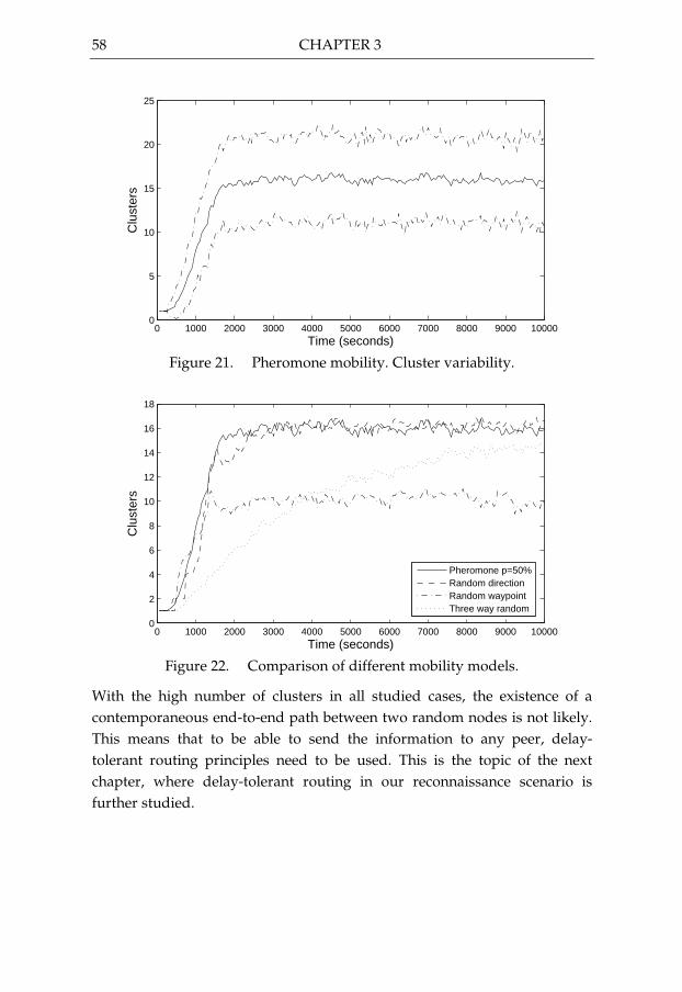
58 CHAPTER 3
0 1000 2000 3000 4000 5000 6000 7000 8000 9000 100000
5
10
15
20
25
Time (seconds)
Clu
ster
s
Figure 21. Pheromone mobility. Cluster variability.
0 1000 2000 3000 4000 5000 6000 7000 8000 9000 100000
2
4
6
8
10
12
14
16
18
Time (seconds)
Clu
ster
s
Pheromone p=50%Random directionRandom waypointThree way random
Figure 22. Comparison of different mobility models.
With the high number of clusters in all studied cases, the existence of a contemporaneous end-to-end path between two random nodes is not likely. This means that to be able to send the information to any peer, delay-tolerant routing principles need to be used. This is the topic of the next chapter, where delay-tolerant routing in our reconnaissance scenario is further studied.

59
4 Routing in IC-MANETs Routing, that is selecting a path for a packet from source to destination, is a challenging task when the network topology is partially unknown to the nodes performing the routing. The disconnected nature of an IC-MANET prevents changes of the network topology from propagating outside the cluster where the change occurred. This means that routing decisions have to be made with imperfect knowledge using heuristic methods. In this chapter we describe and evaluate our proposed geographic routing algorithm Location Aware Routing for Opportunistic Delay-tolerant networks (LAROD) and the Location Dissemination Service (LoDiS), a location service for IC-MANETs. In the evaluations we compare LAROD-LoDiS to Spray and Wait [95][97], a leading delay-tolerant routing algorithm. à Ã Ä
ü ý Ò þ ÿLAROD is a geographic routing protocol for IC-MANETs that combines geographic beacon-less routing, used by MANET routing protocols such as BLR [35] and CBF [27], with the store-carry-forward principle [13]. In its essence LAROD uses greedy packet forwarding when possible, and when greedy forwarding is not possible, the node holding the packet (the custodian) waits until node mobility makes it possible to resume greedy forwarding. To obtain the location of the destination LAROD inquires a location service. Due to the known difficulty of distributing location information in IC-MANETs, LAROD assumes that the provided location data is an approximation of the destination’s current position. To improve the location information LAROD continuously updates the destination’s location data during routing by inquiring the location services in the nodes that route the packet.
For the same reasons as presented in RFC 4838 [13] (see Section 2.1), LAROD uses custody transfer to guarantee reliable delivery of packets. When a packet is generated the LAROD agent in the source node takes custody of the packet, and it only relinquishes this responsibility when it

60 CHAPTER 4
knows that the LAROD agent in another node has taken over custody of the packet. Due to the uncertain signaling in wireless networks it is possible that the current custodian is not informed that a new node has taken custody of the packet. To minimize the impact of these events, LAROD contains logic that purges duplicate copies when their paths cross.
Being a beacon-less routing protocol, LAROD cannot explicitly select the next custodian. Instead of explicit selection LAROD selects the next custodian using timer-based bids. To forward a message towards the destination a custodian simply broadcasts the message. All nodes within a predefined forwarding area (see Figure 23 for examples) are eligible to take over custody of the packet, and are called potential custodians. The potential custodians that actually receive a transmitted packet are called tentative custodians. All tentative custodians set a delay timer (td), specific for each node, and the node whose delay timer expires first is the selected new custodian. Upon becoming a custodian the node forwards the message in the same manner as the previous custodian. The old custodian that sent the message and most other tentative custodians will overhear this transmission and conclude that a new node has taken over custody of the packet. If no such transmission is heard the current custodian regularly (every tr) broadcasts the message until a new custodian becomes available due to node mobility. It is possible that not all nodes in the forwarding area will overhear the broadcast made by the new custodian thereby producing packet duplicates. This will increase the load in the system, but also enable exploration of multiple paths to the destination. When the paths of two copies cross, only one copy will continue to be forwarded. To prevent a packet from indefinitely trying to find a path to its destination all packets have a time to live (tTTL) expressed as a duration. When the TTL expires a packet is deleted by its custodian.
The forwarding area can have many shapes, but it should be designed in such a way that progress towards the destination is guaranteed. All of the space covered by the forwarding area must also provide a positive solution to the selected delay timer function (details will be provided later in this section). An attractive property is the potential for all nodes within the forwarding area to hear each other’s transmissions. This will reduce the risk of tentative custodians failing to receive the packet transmitted by the new custodian. Examples of shapes that meet these criteria are a 60° circle sector, a Reuleaux triangle, or a circle (see Figure 23a-c). The longest distance between two points within these shapes must be the assumed radio range. If

ROUTING IN IC-MANETS 61
overhearing is not a critical property, and we want to maximize the probability of finding a new custodian, then the forwarding area should include all nodes that guarantee progress towards the destination (see Figure 23d. To avoid too small hops and to cater for inaccuracies in the positioning service, e.g the Global Positioning System (GPS), a minimum forward distance may be prudent (the small gap between the custodian and the forwarding area in Figure 23d. All the illustrated forwarding areas can be used in LAROD as a parameterized input and they are compatible with the delay time functions proposed below. For the evaluations we have chosen to use the progress forwarding area. The rationale for this choice will be provided in Section 4.3.2.
Custodian
Sector(a)
Custodian
Reuleaux(b)
Custodian
Circle(c)
Custodian
Progress(d)
Figure 23. Forwarding area examples
While the forwarding area determines the nodes that can become a new custodian, the function that selects the node within the set to be the next custodian is the delay timer function. All potential custodians that receive a packet from a custodian (and thus becomes tentative custodians) set a delay timer (td). The tentative custodian whose timer expires first is the selected new custodian. The delay timer (td) for each node can be set based on many principles, where two natural ones are to favor short hops or long hops towards the destination. Short hops are advantageous if much data is to be exchanged between the nodes since the transfer probability is higher with a shorter distance. The downside is that more hops create higher overhead. Long hops will reduce the number of hops, but the downside is that the transfer reliability between distant nodes is lower which means that the current custodian might not overhear the new custodian’s transmission. As a middle ground one can consider a delay timer that prioritizes nodes at some set distance from the custodian. Implementations of these thee principles are provided in Equations (4.1) – short hops, (4.2) – medium and (4.3) – long hops. Graphical illustrations of these delay functions are provided in Figure 24 (r is the nominal radio range). The gray area for the long hops indicates that the delay is randomized for these distances. For a definition of the terms and default values in the equations see Table 10 and Figure 25. In LAROD any delay timer function that produce positive delays

62 CHAPTER 4
within the forwarding area can be used as it is a configuration parameter. For the evaluations we have chosen to use long hops. The rationale for this choice will be provided in Section 4.3.2.
0 r0
Distance
Del
ay ti
mer
Short hops
0 r0
DistanceD
elay
tim
er
Medium hops
0 r0
Distance
Del
ay ti
mer
Long hops
Figure 24. Delay curve examples
The delay equations are quite straight forward, but the long hops (4.3) warrants some additional comments. It is generally undesirable that several nodes have exactly the same delay time. The reason for this is that, depending on MAC protocol, it increases the risk for garbled transmissions due to nodes transmitting simultaneously. This is normally not a problem since the probability that two tentative custodians are at a similar distance from the custodian is low. For the long hops this becomes a problem if a linear function is used since this means that all nodes beyond a certain point would get a delay time of 0. In a real setting it is an issue since the actual maximum transmission distance varies. To cope with this we have used a linear delay until an end point (l). Tentative custodians beyond the linear end point randomize their delay in such a way that it is guaranteed to be smaller than the linear delay. For these tentative custodians no priority is given based on distance to destination. The linear end point (l) should be set close to the nominal or expected radio range. Another issue that has to be addressed is when a custodian is close to the destination since the normal delay function then gives unsuitable delays. For this reason when the custodian is within l of the destination the tentative custodians use the actual distance to the destination to compute the td. The three parts of equation (4.3) are then as follows.
1. The tentative custodian is within communication range of the destination. Use a linear delay based on distance to the destination.
2. The tentative custodian is beyond the linear end point. Use a random delay.
3. The tentative custodian is within the linear end point. Use a linear delay based on progress towards the destination.

ROUTING IN IC-MANETS 63
Table 10. LAROD parameters
Parameter Description Default value
d Distance between custodian and the destination
-
f Distance between tentative custodian and the destination
-
l Linear end point 240 meters p Minimum progress 10 meters r Nominal radio range 250 meters tl Maximum linear delay 0.8 seconds tm Maximum delay within nominal radio
range 1.0 second
tn Maximum random delay 0.2 seconds z Zero delay distance for medium hops 125 meters X Uniform random variable in range [0,1] -
Custodian
TentativeCustodian
Destination
p
lr
d
f
Figure 25. Delay time parameters illustration
( ) rtfdt md ⋅−= (4.1)
( ) ( )
( ) ( )����� >−
−⋅−
−⋅−
≤−+−⋅−=
zfdzr
zt
zr
tfd
zfdtz
tfd
tmm
mm
d (4.2)
( )( )��������
�+⋅−−
≥−⋅Χ
≤⋅
=
otherwisenl
n
l
d
ttl
fdl
lfdt
ldtl
f
t (4.3)

64 CHAPTER 4
One could argue that the delay timer function should prioritize nodes that move towards the destination. The reason for this selection priority would be that packets are handed over to nodes that will carry it towards the destination. The reason that we have not taken the direction of travel into account when selecting the next custodian is that even if the new custodian might move in the wrong direction, the hope is that it can forward the packet to a node closer to the destination. Another reason is that node directions are not stable and a node might turn and move towards the destination. For these reasons a packet is always forwarded towards the destination as far as possible, even if it in some cases might mean that the packet is returned to a previous custodian due to node movement.
If a custodian could not find a new custodian closer to the destination, it will make a new attempt after some time. This time, the LAROD rebroadcast time (tr), can be set in many ways but the following two guidelines should be used. The time should be short enough that forwarding opportunities are not missed, but it should also be as long as possible to limit bandwidth waste. Currently there is one rebroadcast time function implemented for LAROD and that is a random selection between two configurable times. The reason to use a random selection is that it prevents repeated interference between nodes that are custodians for different packets. For the evaluation of LAROD tr is selected between the valued 8 and 12 seconds. This corresponds to a node moving between 4.5% and 6.7% of the nominal radio range. If LAROD is used in an inhomogeneous system then a more dynamic setting of the LAROD rebroadcast time can be considered. Factors that could influence tr are node speed, number of neighbors and amount of traffic.
To stop further transmission of a packet when it has been delivered to the destination, an acknowledgement packet is sent by the destination at packet reception. An acknowledgement packet is not intended as a delivery receipt to the source, it is only used to prevent further forwarding attempts by nodes holding the acknowledged packet. Upon receipt of an acknowledgement packet a node discards the corresponding data packet, if it has one, and it stores the acknowledgement information for the remaining portion of the packet TTL. Further forwarding of an acknowledgement packet is only done when a node receives a packet for which it previously has received an acknowledgement. It then broadcasts the acknowledgement to stop the transmission of the packet.
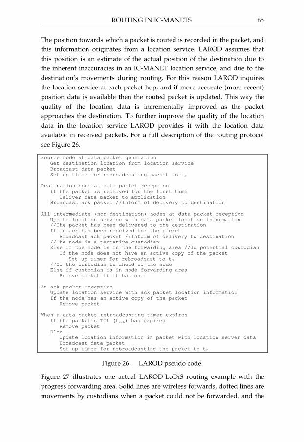
ROUTING IN IC-MANETS 65
The position towards which a packet is routed is recorded in the packet, and this information originates from a location service. LAROD assumes that this position is an estimate of the actual position of the destination due to the inherent inaccuracies in an IC-MANET location service, and due to the destination’s movements during routing. For this reason LAROD inquires the location service at each packet hop, and if more accurate (more recent) position data is available then the routed packet is updated. This way the quality of the location data is incrementally improved as the packet approaches the destination. To further improve the quality of the location data in the location service LAROD provides it with the location data available in received packets. For a full description of the routing protocol see Figure 26.
Source node at data packet generation Get destination location from location service Broadcast data packet Set up timer for rebroadcasting packet to t r Destination node at data packet reception If the packet is received for the first time Deliver data packet to application Broadcast ack packet //Inform of delivery to destin ation All intermediate (non-destination) nodes at data pac ket reception Update location service with data packet location i nformation //The packet has been delivered to the destination If an ack has been received for the packet Broadcast ack packet //Inform of delivery to desti nation //The node is a tentative custodian Else if the node is in the forwarding area //Is pot ential custodian If the node does not have an active copy of the pa cket Set up timer for rebroadcast to t d //If the custodian is ahead of the node Else if custodian is in node forwarding area Remove packet if it has one At ack packet reception Update location service with ack packet location in formation If the node has an active copy of the packet Remove packet When a data packet rebroadcasting timer expires If the packet’s TTL (t TTL) has expired Remove packet Else Update location information in packet with locatio n server data Broadcast data packet Set up timer for rebroadcasting the packet to t r
Figure 26. LAROD pseudo code.
Figure 27 illustrates one actual LAROD-LoDiS routing example with the progress forwarding area. Solid lines are wireless forwards, dotted lines are movements by custodians when a packet could not be forwarded, and the
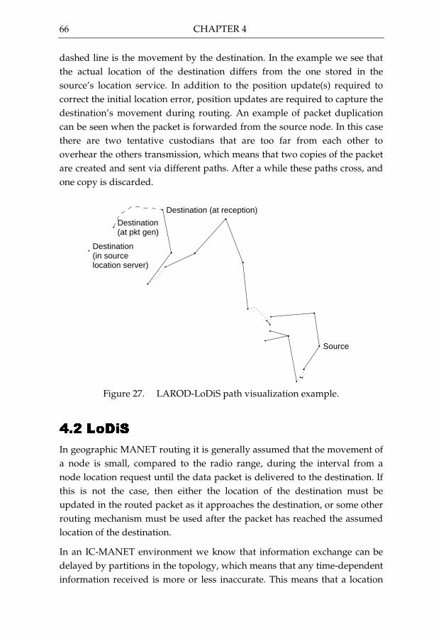
66 CHAPTER 4
dashed line is the movement by the destination. In the example we see that the actual location of the destination differs from the one stored in the source’s location service. In addition to the position update(s) required to correct the initial location error, position updates are required to capture the destination’s movement during routing. An example of packet duplication can be seen when the packet is forwarded from the source node. In this case there are two tentative custodians that are too far from each other to overhear the others transmission, which means that two copies of the packet are created and sent via different paths. After a while these paths cross, and one copy is discarded.
Source
Destination (at reception)
Destination(at pkt gen)
Destination(in sourcelocation server)
Figure 27. LAROD-LoDiS path visualization example. à Ã Í
ü Ì ÿ Ë ÅIn geographic MANET routing it is generally assumed that the movement of a node is small, compared to the radio range, during the interval from a node location request until the data packet is delivered to the destination. If this is not the case, then either the location of the destination must be updated in the routed packet as it approaches the destination, or some other routing mechanism must be used after the packet has reached the assumed location of the destination.
In an IC-MANET environment we know that information exchange can be delayed by partitions in the topology, which means that any time-dependent information received is more or less inaccurate. This means that a location

ROUTING IN IC-MANETS 67
service in an IC-MANET will generally only provide inaccurate location information due to the time taken for a location update to reach the server and/or the time taken for a location request to be answered by a location service. These issues force a designer of a location service in an IC-MANET to decide on how to manage the location errors that the system will inevitably have. æ å ò å ç
� ó ï í õ è � ð í ô í é í úLoDiS is a fully distributed location service, i.e. every node is a location server and location data is updated by data exchanges as nodes encounter each other. The reason that all nodes are location servers is to avoid delaying the packet at the source node. If only a limited set of nodes were location servers then the transmission of a data packet would be delayed by the time it takes for a location server to respond to the location request. Due to the disconnected nature of IC-MANETs this delay could be long. With the low cost of memory, maintaining location tables that contain data on all nodes in the system should not be a problem in a UAV even for fairly large systems (thousands of nodes). If we assume that each location entry requires 30 bytes then 1000 nodes would require 30 kbytes, a very small requirement by modern standards.
Due to the difficulty of distributing timely information in IC-MANETs, LoDiS does not guarantee that the location information it provides is fresh. This limitation has to be taken into account by the routing protocol using LoDiS. When LoDiS provides location data for a node, it also provides the time when the data was accurate. One way a routing protocol can use this information (and this is what LAROD does) is to initially route the packet towards the provided position. During the routing, the routing protocol can inquire the LoDiS service in each node that the packet passes, and if a more accurate (recent) information is available, then the destinations position is updated in the routed packet. Since the nodes that are closer to the destination should have better information on the destination’s location, the accuracy of the destination’s position is incrementally increased. This position update approach does to some extent, resemble the query routing in Brownian Gossip [17]. While Brownian Gossip uses the distributed location information to guide location queries towards the destination, LAROD-LoDiS uses the location information to route the actual data packets due to the disconnected nature of IC-MANETs.

68 CHAPTER 4
LoDiS builds on the conceptual solution used by SLS [12] and employs the principle of MANET broadcast gossip [26] to distribute the continuously changing location data. A LoDiS location server regularly broadcasts the information it has in its location table. Any node receiving this broadcast merges the information with the one it has itself, and the most recent information will be propagated when that node makes its LoDiS broadcast. Thus, location information spreads like rings on water. In addition to the broadcasts, LoDiS also accepts location updates from the routing protocol. The routing protocol will have some location information in the packets that it routes, which could further improve the data in the location service. The pseudo code for LoDiS is shown in Figure 28.
To limit the overhead generated by LoDiS each node is only allowed to generate one packet worth of location data from its location table at a set rate. If we assume a packet size of 1000 bytes and that 10 bytes are required for each node (which includes some compression) then an update can transfer information on 100 nodes. If all location information stored in the node can fit in one packet, then all is well. If that is not the case then a selection has to be made. The selection could range from simple round-robin algorithms, to a selection based on distance and information age. In the results presented in this thesis the number of nodes has been less than the data limit in a packet, and the use of different selection techniques has not been explored. The reason to have a fixed broadcast interval is that it will limit the per node overhead. If a dynamic interval would be used then it should be influenced by factors such as, how often the neighbors change, the number of neighbors, and the amount of new data to be distributed. As an example, Brownian Gossip approximates these factors with the speed of the node. In Section 4.3.3 we will show that the overhead introduced by LoDiS is small compared to the routing overhead from LAROD.
There are several reasons why we have chosen to regularly broadcast the location data instead of using an exchange each time two nodes meet. If an encounter exchange scheme is chosen then the nodes need to broadcast regular beacon messages instead of location data broadcasts. When a beacon message is received a node needs to determine whether it is a new encounter or not, and if it is, initiate an information exchange. This is a more complicated scheme, and it also has the drawback that the exchange may not be finished properly due to node movement, or changed transmission conditions [36]. With the broadcast technique, if the data is received by a node then all is fine and well, and if it is not, then the information will be
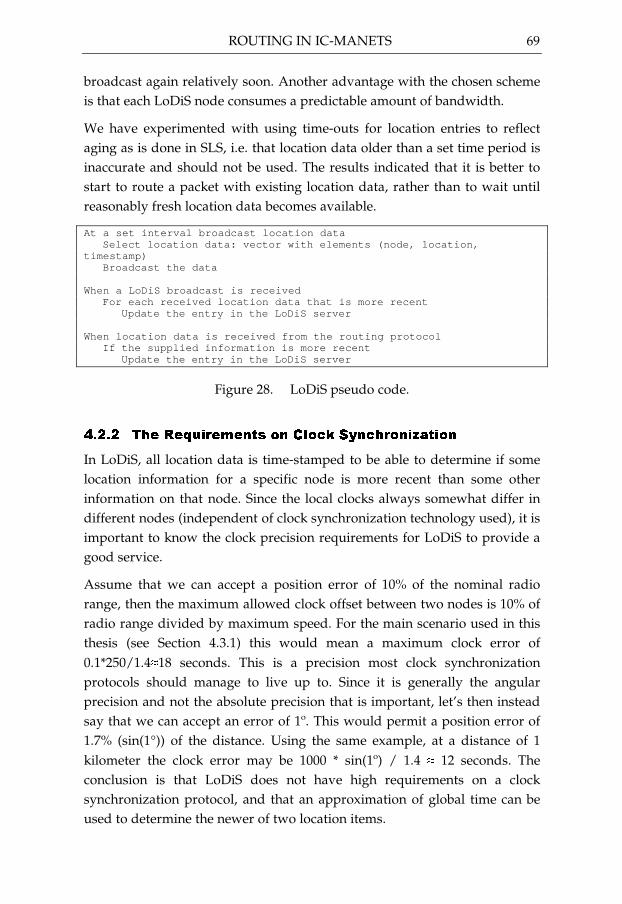
ROUTING IN IC-MANETS 69
broadcast again relatively soon. Another advantage with the chosen scheme is that each LoDiS node consumes a predictable amount of bandwidth.
We have experimented with using time-outs for location entries to reflect aging as is done in SLS, i.e. that location data older than a set time period is inaccurate and should not be used. The results indicated that it is better to start to route a packet with existing location data, rather than to wait until reasonably fresh location data becomes available.
At a set interval broadcast location data Select location data: vector with elements (node, l ocation, timestamp) Broadcast the data When a LoDiS broadcast is received For each received location data that is more recent Update the entry in the LoDiS server When location data is received from the routing prot ocol If the supplied information is more recent Update the entry in the LoDiS server
Figure 28. LoDiS pseudo code. æ å ò å ò � ó ï � ï ø õ ð ï ÷ ï ë ô ö í ë ì ú í é � è � ë é ó ð í ë õ � ê ô õ í ë
In LoDiS, all location data is time-stamped to be able to determine if some location information for a specific node is more recent than some other information on that node. Since the local clocks always somewhat differ in different nodes (independent of clock synchronization technology used), it is important to know the clock precision requirements for LoDiS to provide a good service.
Assume that we can accept a position error of 10% of the nominal radio range, then the maximum allowed clock offset between two nodes is 10% of radio range divided by maximum speed. For the main scenario used in this thesis (see Section 4.3.1) this would mean a maximum clock error of 0.1*250/1.4� 18 seconds. This is a precision most clock synchronization protocols should manage to live up to. Since it is generally the angular precision and not the absolute precision that is important, let’s then instead say that we can accept an error of 1º. This would permit a position error of 1.7% (sin(1°)) of the distance. Using the same example, at a distance of 1 kilometer the clock error may be 1000 * sin(1º) / 1.4 � 12 seconds. The conclusion is that LoDiS does not have high requirements on a clock synchronization protocol, and that an approximation of global time can be used to determine the newer of two location items.

70 CHAPTER 4
à Ã Â á â É × ã É Ø Ë Ì È
In this section, we present the results from our evaluations of LAROD-LoDiS. The routing protocols have been evaluated in the network simulator ns-2 using both the pheromone reconnaissance mobility model and the random waypoint mobility model (for comparative purposes). The setup of the simulator for the evaluations is detailed in Section 4.3.1. In Section 4.3.2 the LAROD parameter options are studied and in Section 4.3.3 the properties of LoDiS are studied and compared to a perfect location service. This is followed in Section 4.3.4 by an evaluation of how the choice of mobility model impacts LAROD-LoDiS. Finally, in Section 4.3.5 we compare the performance of LAROD-LoDiS to Spray and Wait.
The two main evaluation metrics used are delivery ratio and effort required for each generated data packet (overhead). The delivery ratio is the most important evaluation criteria since it determines the quality of service as perceived by the user or application. The effort used to transfer a packet is also important since lean protocols will allow either a higher throughput or lower power consumption by the nodes. This will be measured as the number of transmissions performed per generated data packet. æ å ä å ç
è é ï ë ê ð õ í � ê ð ê ÷ ï ô ï ð ö ê ë � è ï ô � ùThe basic simulation parameters are given in Table 11. The real-world parameters are based on reasonable assumptions made by UAV domain experts. For our simulations in ns-2 we have chosen to keep the default ns-2 radio range and scale the other parameters accordingly to ease comparisons with other work. For the random waypoint mobility model we have used two speed settings; slow and fast. We have used both a constant speed of 1.4 m/s (slow) to match the pheromone reconnaissance mobility model and a variable speed between 1.0 and 10.0 m/s (fast). The variable speed setting is similar to what is used in many MANET simulations.

ROUTING IN IC-MANETS 71
Table 11. Basic simulation parameters
Parameter Real-world ns-2
Reconnaissance area 64x64 kilometers 2000x2000 meters Node density 0.020 nodes/km²,
node degree 3.93 20 nodes/km², node degree 3.93
Node speed 161 km/h 1.4 m/s Radio range 8000 meters 250 meters Data generation rate 36 pkt/hour/node 36 pkt/hour/node Packet life time (TTL) 1000 seconds 1000 seconds
The node density is a very important parameter since, together with the mobility model, it determines how well connected the system is. There is no right or wrong when it comes to node densities and as detailed in Table 4 in Section 2.5, a wide range of relative densities have been used by various researchers. The default node density at which LAROD-LoDiS is evaluated produces small groups of connected nodes (clusters). The chosen node density is below the percolation threshold, meaning that it is very likely that no large dominating clusters exist at any point in time. In particular, we are still at a degree of connectedness that is comparable to some literature in the DTN area (see Table 4 in Section 2.5).
For data generation we have chosen that all nodes generate data packets at a set average rate, and send each of them to a randomly chosen destination. The reason for this abstract communication setup is that it challenges the routing protocol to provide communication paths between all pairs of nodes.
To get as relevant results as possible from the simulations, data should only be collected during system steady state unless initiation and startup phenomena shall be studied. To come as close as possible to this ideal state the data presented in the results below are collected during 3600 seconds at full network activity and with the mobility models at steady state. To guarantee full network activity during the measurement period, the simulation was run at least 1400 seconds (maximum packet life time) before and after the measurement period. When evaluating LAROD-LoDiS the simulation was run for 3600 seconds before the data collection interval to populate the LoDiS location data.
For simulations with the random waypoint mobility model, node position, speed, and initial destination have been initiated according to the procedures and equations proposed by Navidi and Camp [69]. For the pheromone mobility model the nodes have initially been uniformly

72 CHAPTER 4
randomly distributed and then the simulation was run for 3600 seconds before the data collection interval to populate the pheromone maps. For all data points 10 runs have been recorded and the average value is presented. For most curves the 95% confidence interval is also plotted. æ å ä å ò
� � � � ê ð ê ÷ ï ô ï ð öThe performance of LAROD is influenced by the forwarding area and the delay timer. To evaluate the impact of these parameters we evaluated LAROD with two different forwarding areas and two different delay timer functions. In Table 12 we show the delivery ratio for the different settings. We note that while the delivery ratio is greatly impacted by the forwarding area, it is only marginally impacted by the delay timer function. The reason for this is the low node density dictated by our application. The larger area used by the progress area (see Figure 23) means that the probability of finding a node that can forward a packet is larger than for the smaller circle area.
Table 13 shows the overhead of LAROD for the forwarding areas and timers as the average number of transmitted packets per generated data packet. Here, we see that the choice of the timer indeed matters. In the progress area the difference between selecting the closest and the furthest node is seen with the increased overhead for the short hops compared to the long hops. For the circle area both delay functions give similar overhead. The reason for this is that the low node density gives a low probability to have more than one node within the circle forwarding area, which means that irrespective of delay function the same node will be selected. For the rest of the evaluations we have used the progress forwarding area and the long hop delay timer.
Table 12. Delivery ratio for different LAROD parameters.
Forwarding area Short hops Long hops
Circle 86.1%±4.3% 86.8%±6.0% Progress 98.1%±1.7% 97.5%±1.8%
Table 13. Overhead for different LAROD parameters (transmissions per data packet).
Forwarding area Short hops Long hops
Circle 64.6±5.7 61.5±7.8 Progress 53.4±4.9 45.3±5.8

ROUTING IN IC-MANETS 73
æ å ä å ä í õ è � ê ð ê ÷ ï ô ï ð ö ê ë � � ï ð � í ð ÷ ê ë é ï
The major configuration parameter for LoDiS is the broadcast interval. Figure 29 shows the delivery rate of LAROD using LoDiS with four different broadcast intervals from 5 to 100 seconds, and LAROD using an oracle location service. The oracle location service is a perfect baseline since it simulates the case where the location service information is always correct. It is very interesting to note that delivery ratio is essentially identical for all configurations. In simulations with the random waypoint mobility model we got the same type of results. This somewhat surprising result can be explained by the fact that geographic routing can cope with positional errors as long as the angular error is low.
200 400 600 800 1000 1200 14000.5
0.6
0.7
0.8
0.9
1
Packet life time (s)
Del
iver
y ra
tio
LAROD−LoDiS 5LAROD−LoDiS 15LAROD−LoDiS 40LAROD−LoDiS 100LAROD−Oracle
Figure 29. Delivery ratio with parameterized LoDiS and Pheromone
mobility.
Figure 30 plots the overhead of LAROD-LoDiS under the pheromone mobility with different packet life times and broadcast intervals. Not unexpectedly we find that having a longer broadcast interval decreases the transmissions generated by a packet. Each curve shows the overhead with a given broadcast interval (5 seconds, 15 seconds, etc). The variance analysis (not shown here) shows that there is no statistically significant difference between the overheads at the broadcast intervals 15, 40 and 100 seconds. At some point the error introduced by having long broadcast intervals means that the routing will require more transmissions since the packet is routed for too long in the wrong direction. This has been confirmed in evaluations with a broadcast interval of 300 seconds and where location service updates

74 CHAPTER 4
from the routing protocol were not used. For these reasons we have chosen to use a LoDiS broadcast interval of 40 seconds for the rest of the presented results. This is the same interval we use for the Spray and Wait beaconing (see Appendix 2). We have also evaluated LoDiS in a sparser network, and the relative performance results for a node degree of 1.96 were the same as for a node degree of 3.93 (graphs not shown).
200 400 600 800 1000 1200 14000
10
20
30
40
50
60
Packet life time (s)
Tra
nsm
issi
ons
per
data
pac
ket
LAROD−LoDiS 5LAROD−LoDiS 15LAROD−LoDiS 40LAROD−LoDiS 100LAROD−Oracle
Figure 30. Overhead with parameterized LoDiS and Pheromone mobility.
In a geographic routing protocol, is not always important to know exactly where the destination is, but to know approximately the direction to the destination. As a packet moves closer to the destination the position information can be updated by intermediate routers to a more accurate position for the final routing steps. In Figure 31 the average direction error at the source node for different LoDiS broadcast intervals is plotted. Not unexpectedly the error increases with longer broadcast intervals, but for all scenarios except for the fast random waypoint the error is small (below 11°), which means that the packets will be sent in the right direction. With a very long broadcast interval of 300 seconds, and with no location service updates from the routing protocol, an average direction error of 29° was measured together with a significant drop in the delivery ratio. Due to the more disconnected nature of the pheromone mobility compared to random waypoint mobility, location distribution takes more time, and for this reason the direction error is larger for pheromone mobility with a comparable speed profile. This indicates the challenging nature of the pheromone reconnaissance mobility model which is induced by the application scenario.

ROUTING IN IC-MANETS 75
Analysis of the distribution data for all runs shows that for the pheromone mobility scenario 94% of the packets are sent with an angle error of less than ±20º. For the slow random waypoint scenario the value is 98% and for the fast 86%.
These results show that the overhead (cost) of LoDiS is low compared to an oracle location service, and that the impact on delivery ratio due to location errors is insignificant. We have also shown that the directional error when a packet is sent from its source is low, which partially explains the good overall results.
0 10 20 30 40 50 60 70 80 90 1000
5
10
15
LoDiS broadcast interval (s)
Ang
le e
rror
(de
gree
s)
PheromoneRwp fastRwp slow
Figure 31. Average direction error at source node. æ å ä å æ
� ó ï � ÷ ù ê é ô í � ô ó ï � í � õ ú õ ô � � í � ï úEvaluating the routing protocols under three different mobility scenarios reveals the importance of selecting a relevant scenario when studying a routing protocol. In Figure 32 we see the impact of the delivery ratio for LAROD-LoDiS for the pheromone reconnaissance mobility model, and the random waypoint mobility model with two speed profiles. All scenarios have the same average node density as defined in Table 11, but the difference in node distribution, movement pattern and movement speed greatly impacts the results. The overhead for the same setup is shown in Figure 33. Not unexpectedly the overhead increases for the scenarios with a lower delivery ratio. The reason is that more packets live longer before they either reach their destination, or time out.

76 CHAPTER 4
200 400 600 800 1000 1200 14000.5
0.6
0.7
0.8
0.9
1
Packet life time (s)
Del
iver
y ra
tio
Rwp fastRwp slowPheromone
Figure 32. LADOD-LoDiS delivery ratio for different scenarios.
200 400 600 800 1000 1200 14000
5
10
15
20
25
30
35
40
45
50
55
Packet life time (s)
Tra
nsm
issi
ons
per
data
pac
ket
Rwp fastRwp slowPheromone
Figure 33. LADOD-LoDiS overhead for different scenarios.
The corresponding results for Spray and Wait with a spray factor of 10 are presented in Figure 34 and Figure 35. What is noteworthy in these graphs is how strongly the result is impacted by the mobility model. As stated by Spyropoulos in [95], Spray and Wait requires that enough nodes that can carry packets roam the entire network. With the random waypoint mobility model nodes more consistently roam the entire area compared to the pheromone reconnaissance mobility model. These results confirm earlier reports [47][63] that the choice of relevant mobility model is important when evaluating routing protocols.

ROUTING IN IC-MANETS 77
200 400 600 800 1000 1200 14000
0.1
0.2
0.3
0.4
0.5
0.6
0.7
0.8
0.9
1
Packet life time (s)
Del
iver
y ra
tio
Rwp fastRwp slowPheromone
Figure 34. Spray and Wait delivery ratio for different scenarios.
200 400 600 800 1000 1200 14000
20
40
60
80
100
120
140
160
180
200
Packet life time (s)
Tra
nsm
issi
ons
per
data
pac
ket
Rwp fastRwp slowPheromone
Figure 35. Spray and Wait overhead for different scenarios. æ å ä å �
� � � � í õ è ì í ÷ ù ê ð ï � ô í è ù ð ê � ê ë � � ê õ ôIn order to show the merit of LAROD-LoDiS compared to other routing schemes we have compared it to Spray and Wait [95][97]. Spray and Wait is reportedly an efficient routing protocol with good delivery properties. It would also be interesting to compare LAROD-LoDiS to another geographic IC-MANET routing protocol. However, since most geographic delay-tolerant routing protocols are designed for road based scenarios, and we have not found any that implement a location service, we have not found it worth the effort to re-implement any of them in ns-2. As Spray and Wait

78 CHAPTER 4
originally was implemented for a custom simulator we have re-implemented it in ns-2. Implementation details are provided in Appendix 2.
Comparing the delivery ratio and overhead of LAROD-LoDiS to Spray and Wait we see that the benefit of using geographic information and active forwarding is very high (see Figure 36 to Figure 39). Under the pheromone reconnaissance mobility model Spray and Wait does not provide an acceptable delivery ratio. In Figure 36 we see the impact of the packet life time on the delivery ratio. As expected both routing protocols benefit from having more time to find a path from source to destination. The relative performance of the two protocols is not surprising since Spray and Wait mainly uses node mobility to forward packets while LAROD actively forwards the packet via peers towards the destination. As long as node encounters are frequent then protocols that actively forward should outperform protocols relying on node mobility as the main delivery mechanism. What is also interesting to note is that the overhead for Spray and Wait is about double that of LAROD-LoDiS for a spray factor of 10 and almost four times higher with a spray factor of 20 (see Figure 37). A large factor in the Spray and Wait overhead are the beacons and the query and response packets, packets not present in LAROD-LoDiS.
200 400 600 800 1000 1200 14000
0.1
0.2
0.3
0.4
0.5
0.6
0.7
0.8
0.9
1
Packet life time (s)
Del
iver
y ra
tio
LAROD−LoDiSSpray and Wait L=20Spray and Wait L=10
Figure 36. Delivery ratio for different packet life times under pheromone
mobility.

ROUTING IN IC-MANETS 79
200 400 600 800 1000 1200 14000
20
40
60
80
100
120
140
160
Packet life time (s)
Tra
nsm
issi
ons
per
data
pac
ket
LAROD−LoDiSSpray and Wait L=20Spray and Wait L=10
Figure 37. Overhead for different packet life times under pheromone
mobility.
Comparing the two routing protocols with respect to varying load we see that both LAROD-LoDiS and Spray and Wait with 10 copies maintain a constant delivery ratio meaning that neither routing protocol overloads the network over a wide load spectrum (see Figure 38). However, increasing the Spray and Wait spray factor to 20 packets, we see that the system becomes overloaded and the delivery ratio drops.
Looking at the overhead in Figure 39 we observe that the overhead for LAROD-LoDiS is essentially constant for varying load. The reason is that the transmissions from LAROD are proportional to the number of generated packets. Also, the node-linear overhead from LoDiS is so low that amortizing it is hardly noticeable. For Spray and Wait the overhead per generated packet is reduced with increased load as the query exchanges are amortized over more data packets.

80 CHAPTER 4
20 40 60 80 100 1200.4
0.5
0.6
0.7
0.8
0.9
1
Load (pkt/hour/UAV)
Del
iver
y ra
tio
LAROD−LoDiSSpray and Wait L=20Spray and Wait L=10
Figure 38. Delivery ratio for different transmission loads under
pheromone mobility.
20 40 60 80 100 1200
50
100
150
200
Load (pkt/hour/UAV)
Tra
nsm
issi
ons
per
data
pac
ket
LAROD−LoDiSSpray and Wait L=20Spray and Wait L=10
Figure 39. Overhead for different transmission loads under pheromone
mobility.
If we study the performance of the two routing protocols under varying node densities we can make some interesting observations. For both routing protocols the delivery ratio improves with increased node density (see Figure 40), but the change is more pronounced for LAROD-LoDiS than for Spray and Wait. The reason that the delivery ratio for Spray and Wait is only marginally improved with increased node density is that its main routing mechanism, waiting until a node holding the packet meets the destination, is not affected by the node density. The improvement with
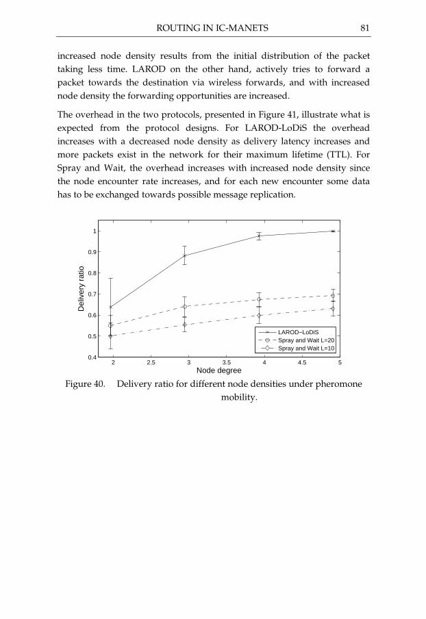
ROUTING IN IC-MANETS 81
increased node density results from the initial distribution of the packet taking less time. LAROD on the other hand, actively tries to forward a packet towards the destination via wireless forwards, and with increased node density the forwarding opportunities are increased.
The overhead in the two protocols, presented in Figure 41, illustrate what is expected from the protocol designs. For LAROD-LoDiS the overhead increases with a decreased node density as delivery latency increases and more packets exist in the network for their maximum lifetime (TTL). For Spray and Wait, the overhead increases with increased node density since the node encounter rate increases, and for each new encounter some data has to be exchanged towards possible message replication.
2 2.5 3 3.5 4 4.5 50.4
0.5
0.6
0.7
0.8
0.9
1
Node degree
Del
iver
y ra
tio
LAROD−LoDiSSpray and Wait L=20Spray and Wait L=10
Figure 40. Delivery ratio for different node densities under pheromone
mobility.

82 CHAPTER 4
2 2.5 3 3.5 4 4.5 50
50
100
150
200
Node degree
Tra
nsm
issi
ons
per
data
pac
ket
LAROD−LoDiSSpray and Wait L=20Spray and Wait L=10
Figure 41. Overhead for different node densities under pheromone
mobility. à Ã à � Ì È Æ × ã Ó Ë È � Ò Ç Ô É Ê � Ú
The selection of an IC-MANET routing protocol is not as simple as selecting the one best protocol, simply because such a protocol does not exist. Instead the properties and mobility of the nodes that provide the routing infrastructure determine the suitability of a routing protocol. Spray and Wait works best when the routing nodes roam around in the network and LAROD-LoDiS requires that the network consists of clusters of at least a handful of nodes to use the geographic forwarding with the best effect. The general advice is that a routing protocol shall first be selected after the properties of the routing infrastructure is known and understood, and when the application requirements are known.

83
5 A Framework for Performance Analysis
Simulators, such as ns-2, provide one way to model routing. While intuitive, this type of model most often requires significant computing resources to provide the routing results. More abstract mathematical models generally provide results with less computing effort. Unfortunately, the abstractions used often mean that the results are less valid compared to those from high fidelity simulations.
In this chapter we present and validate our mathematical forward-wait framework. The framework models geographic routing in IC-MANETs as a sequence of alternating forwarding and waiting phases. As an input, the framework requires the statistical properties of these phases. These characteristics can be derived from multiple sources: models, simulations, or practical data. The quality of the prediction made by the forward-wait framework depends heavily on how accurate these descriptions are. Ã Ä
Î Ï Ç ! Ì Ê " É Ê Ó # Ð É Ë Ø ! Ê É Ô Ç " Ì Ê �In the forward-wait framework, the movement of a packet towards the destination is modeled by two phases, forwarding and waiting. The forwarding phase is used to characterize how much closer a packet gets to the destination when it can be forwarded within a cluster in the network. Once forwarding is not possible, the waiting phase accounts for how long time a packet has to wait until it can be forwarded again. While the model is developed for geographic routing, it is agnostic to the routing mechanism used to forward the packet. However, the model does make the following assumptions.
1. Only one copy of a packet is routed at any time.
2. The delivery latency is dominated by the waiting time, and thus the forwarding time can be neglected.

84 CHAPTER 5
3. The packet travel distance is dominated by the forwarding, and thus in the waiting phase, packet movement due to node mobility can be neglected.
In Section 5.5 we will discuss the validity of these assumptions. There we will show the impact of violations of these assumptions, and that the impact can be compensated for to some extent. The reason to defer the discussion until then is the need for data in order to determine the impact of the assumptions.
Figure 42 visualizes assumptions 2 and 3 with two packets moving from source to destination. In a forwarding phase, a packet travels some distance until it has to wait. While forwarding, the elapsed time is ignored by the second assumption above, which is depicted by the horizontal lines in the figure. The waiting phases, on the other hand, ignore node movements, as indicated by the vertical lines. The two cases in the figure illustrate that, when a packet is generated by the source, it either has to wait if the source node is at the edge of a cluster (upper track), or it can be forwarded immediately, within the current cluster, until it reaches the edge (lower track). Thus, a packet will travel in time and space in a manner similar to one of the two tracks depicted in Figure 42.
0 1 2 3 4 5 6 7
0
50
100
150
200
250
300
350
Distance (radio radii)
Tim
e (s
econ
ds)
Forwarding, after no initital waitWaiting, after no initital waitForwarding, after initital waitWaiting, after initital wait
Figure 42. Time-distance forward illustration.
The forwarding and waiting components of the framework are described by independent random variables. In the forwarding phase, the corresponding random variable describes how far a packet can be forwarded until it reaches the edge of its current cluster. In the waiting phase, we use a

A FRAMEWORK FOR PERFORMANCE ANALYSIS 85
random variable to describe how long time it takes until node movements have restructured the topology in such a way that the packet can be forwarded again. The reason that independence between the random variables can be assumed is that, as a packet is forwarded, it is handled by new nodes whose movements are independent of the nodes previously holding the packet. Examples of how the properties of the random variables can be derived for a specific scenario are provided in Section 5.2. In the same section, we show why it is important to separate two cases, depending on whether or not a packet had to wait at the source or not before it could be forwarded.
The mathematical description of the framework will now be presented in a bottom-up fashion. As a final outcome, we will have the probability of reaching the destination at a distance d within time t, Pd(t,d), the delivery ratio for a specific scenario, PTTL(t), and random variables describing the distance a packet has travelled at a specific time, X(t), and the time it took to travel a specific distance T(d). All results are derived based on the random variables describing the forwarding and waiting phases. In Table 14, we summarize the key notation and terms.
Table 14. Key notation and terms
Notation Description
d Distance t Time L Random variable describing the distance forwarded from the
source during the first forwarding phase, if the packet could be forwarded immediately when it was generated
Ln Random variable describing the distance forwarded during the nth forwarding phase after waiting, if the packet could be forwarded immediately when it was generated
L'n Random variable describing the distance forwarded during the nth forwarding phase after waiting, if the packet had to wait at the source before forwarding
I Random variable that with 100% probability takes the value 0 Dn Random variable describing the distance forwarded from the
source after n forwarding phases, if the packet could be forwarded immediately when it was generated
D'n Random variable describing the distance forwarded from the source after n forwarding phases, if the packet had to wait at the source before forwarding
Vn Random variable describing the time that a packet is in the nth waiting phase until it can be forwarded
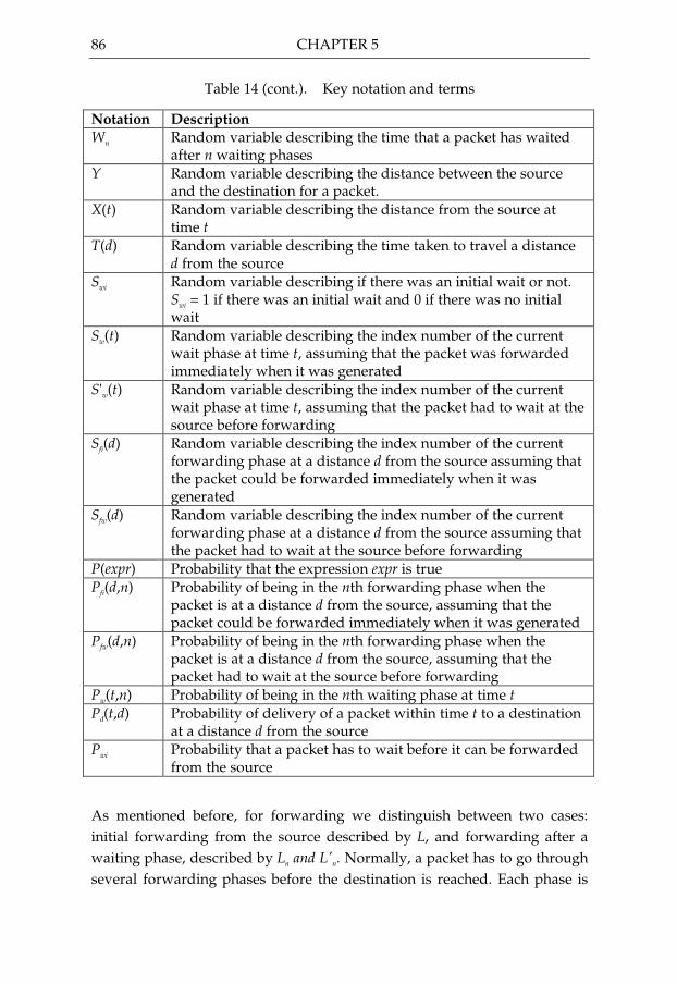
86 CHAPTER 5
Table 14 (cont.). Key notation and terms
Notation Description
Wn Random variable describing the time that a packet has waited after n waiting phases
Y Random variable describing the distance between the source and the destination for a packet.
X(t) Random variable describing the distance from the source at time t
T(d) Random variable describing the time taken to travel a distance d from the source
Swi Random variable describing if there was an initial wait or not. Swi = 1 if there was an initial wait and 0 if there was no initial wait
Sw(t) Random variable describing the index number of the current wait phase at time t, assuming that the packet was forwarded immediately when it was generated
S'w(t) Random variable describing the index number of the current wait phase at time t, assuming that the packet had to wait at the source before forwarding
Sfi(d) Random variable describing the index number of the current forwarding phase at a distance d from the source assuming that the packet could be forwarded immediately when it was generated
Sfw(d) Random variable describing the index number of the current forwarding phase at a distance d from the source assuming that the packet had to wait at the source before forwarding
P(expr) Probability that the expression expr is true Pfi(d,n) Probability of being in the nth forwarding phase when the
packet is at a distance d from the source, assuming that the packet could be forwarded immediately when it was generated
Pfw(d,n) Probability of being in the nth forwarding phase when the packet is at a distance d from the source, assuming that the packet had to wait at the source before forwarding
Pw(t,n) Probability of being in the nth waiting phase at time t Pd(t,d) Probability of delivery of a packet within time t to a destination
at a distance d from the source Pwi Probability that a packet has to wait before it can be forwarded
from the source
As mentioned before, for forwarding we distinguish between two cases: initial forwarding from the source described by L, and forwarding after a waiting phase, described by Ln and L'n. Normally, a packet has to go through several forwarding phases before the destination is reached. Each phase is

A FRAMEWORK FOR PERFORMANCE ANALYSIS 87
described by an independent random variable. The total distance travelled after n forwarding phases is the sum of the random variables. For computing D'n, we also describe the case where no forwarding has taken place. Defining this case is helpful in the description of the final outcome. The resulting random variables Dn and D'n are easily computed by Equations (5.1) and (5.2). $%&
>+=
=− 1
1
1 nLD
nLD
nnn (5.1) '(')*
>′+′=′=
=′
− 1
1
0
1 nLD
nL
nI
D
nn
nn (5.2)
The probability that a packet is in its nth forwarding phase at a distance of d from the source is then given by Equation (5.3). Probability Pfw(d,n) is defined in the same way using D'n. It is important to note that while P(Dn+ d) is the probability of having reached at least a distance d using exactly n forwarding phases, Pfi(d, n) is the probability of being in the nth forwarding phase at distance d. ,-,./ >≥−≥=−≥
=≥=
−
−
=
01)()(),()(
1)(),(
1
1
1
1
ndDPdDPmdPdDP
ndDPndP
nn
n
mfin
fi (5.3)
Similar to the derivation of the random variables for the forwarding phase, Equation (5.4) computes the random variable describing the time of waiting after exactly n waiting phases. Analogous to the definition of D'n, Wn is defined also for the case where no waiting has occurred. In Equation (5.5) we give the probability of being in the nth waiting phase at time t. 12134
>+==
=
− 1
1
0
1 nVW
nV
nI
W
nn
nn (5.4)
56578 >≥−≥=−≥
=≥= 9−
=− 1)()(),()(
1)(),( 1
11
1
ntWPtWPmtPtWP
ntWPntP n
mnnwn
w (5.5)
Using the above results, we can now define expressions predicting routing performance. The main result is presented in Equation (5.6) where we compute the probability that a packet has, within time t, been delivered to a

88 CHAPTER 5
node that is a distance d from the source. The two terms in the equation consider the cases where a packet initially waits before being forwarded, and the case where it is immediately forwarded from the source, respectively. These two cases correspond to the two tracks in Figure 42. Each term is a sum of the probabilities of the possible sequences of forwarding and waiting at the evaluation point. This equation will be used to compute the packet delivery ratio.
( ) ( ) ( ):: ∞
=−
∞
=≤⋅⋅−+≤⋅⋅=
11
1
)(),(1)(),(),(n
nfiwin
nfwwid tWPndPPtWPndPPdtP (5.6)
The probabilistic answer provided by (5.6) might not be enough if a more detailed analysis of the routing performance is to be conducted. To complement Pd(t,d), we define the distance travelled at time t by stochastic variable X(t) in (5.7), and the time required to travel a distance d by stochastic variable T(d) in (5.8). To describe these two properties, we use stochastic variables defining the indices of the forwarding or waiting phase that the packet is in. For the selection of distribution for a particular case we use the Kronecker delta defined as follows. ;<=
≠=
=00
01)(
n
nnδ
Equations (5.7) and (5.8) have the same structure as (5.6), but instead of probabilities, we operate on random variables. Equation (5.7) describes the distance from the source at time t. The first term describes the case when the packet was forwarded after an initial wait, and the second term describes the case for a sequence of forwards without an initial wait. The equation uses selection elements (Swi, Sw(t) and S'w(t)) defined by the following probabilities described earlier.
wiwi PSP == )1(
),())(())(( ' ntPntSPntSP www ====
( ) ( )( )( ) ( ) ( )( )>> ∞
=
∞
=⋅−⋅+⋅−−⋅−=
11
'' )(1)(1)(n
nwwin
nwwi DtSnSDtSnStX δδδδ (5.7)
Equation (5.8) has the same structure as (5.7), but instead computes the time taken to travel a distance d. In addition to Swi the equation uses the selection elements Sfw(d) and Sfi(d) defined by the following probabilities described earlier.

A FRAMEWORK FOR PERFORMANCE ANALYSIS 89
),())(( ndPndSP fwfw ==
),())(())(( ' ntPntSPntSP www ====
( ) ( )( )( ) ( ) ( )( )?? ∞
=
∞
=⋅−⋅+⋅−−⋅−=
11
'' )(1)(1)(n
nwwin
nwwi DtSnSDtSnStX δδδδ (5.8)
To be able to compute the packet delivery ratio, the most commonly used routing metric, we need the source destination distance, Y. With this defined the delivery ratio, PTTL(t), is computed according to Equation (5.9). The equation models the fact that, when a packet is within the radio range of the destination, the last hop is a guaranteed success. @@ ∞
−⋅+=r
d
r
TTL dxrxtPxYpdfdxxYpdftP ),(),(),()(0
(5.9)
The forthcoming sections will be devoted to deriving the properties of the forwarding and waiting random variables in a given context, and validating the model using simulation data. In addition, we will show how Pd(t,d) can be used in a practical application of the framework. A B C
D E F G F H I J G K L K M N O P G Q F G R K M N F M R S F K I K M NIn order to use the framework presented in Section 5.1 for estimating the routing performance with a given mobility model and routing protocol, we need a description of the properties of the random variables for forwarding and waiting. We explore two alternatives: 1) using abstract models for mobility and routing in Section 5.2.2, and 2) using data from a protocol simulation, i.e. LAROD ns-2 simulations presented in Section 4.3, in Section 5.2.3.
The first alternative is useful if the properties of a mobile scenario and routing protocol are well known and can be modeled. The second alternative can capture the distributions of any routing protocol and mobility scenario, including protocols for which the characteristics are not well known. For illustration of the process of creating the abstract model based on a known mobility and routing algorithm we use our knowledge of the LAROD routing protocol, the characteristics of which will be briefly described in Section 5.2.1.

90 CHAPTER 5
In ad hoc wireless networks, distances have little meaning, unless the range capabilities of the chosen radio technology are also specified. For this reason, we have chosen to represent the distance in terms of the multiples of the nominal radio range. Moreover, we will treat node densities by the node degree. T U V U W
X Y Z [ \ ] ^ [ _ ` Y a b a [ c ] d e f ` g [ a d h _ ` e i bIn this section we detail the mobility and routing models used in Section 5.2.2 to derive the model-based forwarding and waiting properties. The model is intended to capture the mobility and routing in the LAROD ns-2 simulations used in Section 5.2.3, but still be manageable so that using the model is significantly simpler than using simulations. T U V U W U W
j ` a Z Z ` d k ] Z i e _ ` Y a b a [ cFor the abstract mobility model we choose the Poisson distribution [33] to describe the statistical distribution of the nodes. The Poisson distribution describes the statistical location properties of independent nodes that are equally likely to be in all locations in an infinite space. The choice of using Poisson distribution is justified by three reasons. First, it is a commonly used abstraction and mathematically attractive. Second, it is a reasonable simplification of the pheromone mobility model that we have used in the ns-2 simulations. Third, it describes the location properties of nodes in some commonly used synthetic mobility models [59][66].
The Poisson distribution only describes how the nodes are statistically distributed, not how they move. To derive the properties of the waiting phase, we need to characterize how the nodes move during a limited time period. To this end, we assume that the nodes move independently at a common constant speed, and that for short time periods the movements can be regarded rectilinear. The common constant speed reflects the speed used in the LAROD ns-2 simulations. T U V U W U V
_ ` e i b a d h l i ` h \ ] m n a ^ f ` g [ a d hMany geographic opportunistic forwarding algorithms are based on forwarding areas, a notion that we use in the model. Since our target is predicting the performance of LAROD, we will use its parameters when modeling routing behavior. To match the configuration choices made in the ns-2 simulations presented in Section 4.3, we model the geographic routing

A FRAMEWORK FOR PERFORMANCE ANALYSIS 91
using the progress forwarding area, see Figure 43, and the retry interval (tr) is uniformly selected between 8 and 12 seconds.
Custodian ForwardingArea
Destination
Figure 43. An illustration of minimum progress forwarding area
Modeling custodian selection in the geographic routing protocol with a minimum progress requirement leads to Equations (5.10) and (5.11), for which the terms are defined in Table 15. Equation (5.10) defines the forwarding area, and (5.11) describes the position of the next custodian. The forwarding operation is characterized by the distance a packet approaches the destination from the current custodian. When a forwarding phase starts, the packet is routed without delay, until forwarding is no longer possible, because the current custodian’s forwarding area is empty. In the waiting phase, the protocol regularly attempts to start a new forwarding.
rXXpXXXXXXfaX cdcddc ≤−+−≤−→∈ ,|)( (5.10)
( ))(|min| dcndnnx XXfaXXXXX →∈−= (5.11)
Table 15. Terms in custodian selection.
Notation Description
r Nominal radio range p Minimum-required progress. The parameter is set to 0.04r. X Two-dimensional Euclidian position Xc Position of the current custodian. Xd Position of the destination. Xn Position of node n. Xx Position of the next custodian. fa(Xco Xd) Forwarding area for a custodian at Xc and destination at Xd.

92 CHAPTER 5
T U V U V p \ ] q i r ` \ s t d m g [ Z k ] Z i e ` d _ ` e i b Z
In this section we will derive the properties for the forwarding and waiting random variables based on the models described in Section 5.2.1. The random variables will be described using distributions (for details see Appendix 4). To see the impact of node density, we will evaluate four different node densities within a relevant range. T U V U V U W
p ` \ r ] \ e a d h u a Z [ \ a Y g [ a ` d k ] Z i e ` d _ ` e i b ZEven for the ideal disc-based transmission model, determining the forwarding distribution analytically for Poisson distributed nodes is unfortunately too complex to be practically tractable. For details, please see Appendix 3. For this reason, we have derived the forwarding cdfs using Monte Carlo simulation.
For determining the distance forwarded from the source (L) the Monte Carlo simulation is set up as follows. A number of nodes drawn from a Poisson distribution are placed in a rectangular area. The area is large enough so that at most 0.1% of the packets will reach the area boundary. Each node’s coordinate is set randomly following a rectangular distribution. A packet is sent towards a destination located infinitely far away, and the forwarding progress, measured along the line connecting the source and destination, is determined. Custodian selection is performed according to (5.10), until an empty forwarding area is encountered.
The result is shown in Figure 3 using the complementary cdf (ccdf) for four different values of node density (where c denotes the node degree defined in Section 2.5). The ccdf in the figure is (1-cdf(L,d))·(1-Pwi), as the Monte Carlo simulations also record the occasions when no node is present in the forwarding area and the packet has to wait. In order to derive a well-behaved density function, the distribution from the Monte Carlo simulation has been fitted to a curve described by (5.12), where G is a gamma-distributed random variable with shape parameter r and scale parameter v . The transition points in (5.12) are selected to achieve an optimal match between the measured distribution and the fitted curve.
Using the assumption of Poisson distributed nodes, the measured probability that a packet could not be forwarded from the source, Pwi, from the Monte Carlo simulations can be theoretically verified. Knowing the node density and forwarding area size the theoretical probability for not

A FRAMEWORK FOR PERFORMANCE ANALYSIS 93
forwarding is trivial to determine (this is the probability that there are no nodes in the forwarding area). For our definition of the forwarding area the results are presented in Table 16. These values are closely matched by the Monte Carlo simulations.
0 5 10 150
0.1
0.2
0.3
0.4
0.5
0.6
0.7
0.8
0.9
1
Forward distance (radio radii)
Dec
umul
ated
pro
babi
lity
c = 5c = 4c = 3c = 2
Figure 44. Probability of being forwarded by at least a given distance from
the source with no initial wait (ccdf), for four node density values.
( )wxwyz >
≤≤⋅+⋅+⋅+<
=3.1),,(
3.104.0
04.00
),( 33
2210
ddrGcdf
ddkdkdkk
d
dLcdf
λ (5.12)
Table 16. Probability of having an initially empty forwarding area
Avg. node degree c
Pwi
2 38.7% 3 24.1% 4 15.0% 5 9.3%
When the packet is forwarded to the edge of a cluster, it has to wait until further forwarding can take place. When at least one node enters the forwarding area this wait ends, and forwarding can continue. The property of this forwarding will not be the same as the forwarding experienced by the source node when the packet was generated. The reason is that a custodian candidate in the forwarding area after a wait will be found close to the edge

94 CHAPTER 5
of the current custodian’s forwarding area. This is due to the fact that the node movements are small during a retry interval compared to the size of the forwarding area. We will see that this will have significant implications for the forwarding distribution.
The Monte Carlo simulations used to determine the distance forwarded after a wait (Ln, L'n) are set up similar to the ones used for analyzing packet forwarding from the source (L). A simulation run starts by placing a number of nodes, drawn from a Poisson distribution, in a rectangular area. Searching through the nodes, the first node having an empty forwarding area is selected to be the custodian of a packet. If no node with an empty forwarding area exists, the simulation run is aborted. Provided that a custodian is found, the next step is to move all the nodes (including the custodian) in random directions for a distance randomly selected to correspond to the retry interval employed between forward attempts (in the abstract model we have used the same interval, 8-12s, as in LAROD ns-2 simulations). If a node has entered the forwarding area after the retry interval, the forwarded distance of the packet is recorded, otherwise the simulation run is discarded.
The resulting distribution is shown in Figure 45 using its ccdf. The figure leads to several interesting observations. The steep drop at the beginning of the curves corresponds to the case that a node enters the forwarding area from the rear. In this case, the forwarding areas of the initial and new custodians have a large overlap. As a result, the probability of making another hop is low. Similar to the cdfs for initial forwarding at the source, the cdfs in Figure 45 have been curve-fitted to derive well-behaved pdfs. The curve fitting is done according to Equation (5.13), where the transition points are selected based on maximum match between the measured distribution and the fitted curve. In the equation, parameters d4 and d5 are density dependent, and selected to achieve an optimal fit.

A FRAMEWORK FOR PERFORMANCE ANALYSIS 95
0 5 10 150
0.1
0.2
0.3
0.4
0.5
0.6
0.7
0.8
0.9
1
Forward distance (radio radii)
Dec
umul
ated
pro
babi
lity
c = 5c = 4c = 3c = 2
Figure 45. Probability of being forwarded by at least a given distance from
the source after a wait (ccdf), for four node density values.
( ){{{{|{{{{}~
>≤<⋅+⋅+⋅+
≤<⋅+⋅+⋅+≤<⋅+⋅+⋅+≤<⋅+⋅+⋅+
≤
==
5
543
332
323130
43
232
222120
313
2121110
33
2210
),,(
85.0
85.016.0
16.004.0
04.00
),'(),(
dddrGcdf
ddddkdkdkk
dddkdkdkk
ddkdkdkk
ddkdkdkk
d
dLcdfdLcdf nn
λ
(5.13)
� � � � � � � � � � � � � � � � � � � � � � � � � � � � � � � � � � � � � � � �
A wait period starts when a packet reaches the edge of a partition where it has to wait until mobility makes further forwarding possible. To determine the distributions for the waiting phase based on the modeled mobility and routing, we consider the periodic forward attempts employed by LAROD. After waiting a time t the probability of successful forwarding is described by Pf(t). With knowledge of when a forward attempt is made, described by R, the waiting distribution can be established. For the LAROD simulations, pdf(R,t) is a rectangular distribution as specified in (5.14). ��� ≤≤
=otherwise
ttRpdf
0
12825.0),( (5.14)
For Pf(t), we note that it is zero at t=0 and equals Pwi as t approaches infinity. Therefore, Pf(t) is expected to have an exponential-type shape. Since we are only interested in Pf(t) when pdf(R,t) is non-zero, a linear approximation is

96 CHAPTER 5
considered. An analysis of the data points used to establish Pf(t) has shown that this is a reasonable approximation over the relevant interval.
The probability of forwarding after a given waiting time (Pf(t)) is not trivial to determine analytically, and for this reason we have used Monte Carlo simulations. In each simulation run, a number of nodes are placed in a rectangular area, following a Poisson distribution. The size of the area is selected such that the expected number of nodes with an empty forwarding area is 100. All nodes are then randomly moved. Whether or not nodes have entered the forwarding areas that were initially empty is then recorded. The simulation has been run for 100 times for each of the time values 8, 9, 10, 11 and 12 seconds, giving approximately 10,000 samples per point. The collected data is then fitted to a linear function to represent Pf(t). The coefficients in the linear function and two sample values are provided in Table 17, and the linear function itself is given in (5.15).
Table 17. Average probability of forwarding after a retry interval.
Avg. node degree c
k o t=8 t=12
2 0.0059 0.013 6.0% 8.3% 3 0.0080 0.023 8.7% 11.9% 4 0.0127 0.008 11.0% 16.1% 5 0.0167 -0.002 13.2% 19,9%
otktPf +⋅=)( (5.15)
What remains is to compute the waiting time Vn based on R and (5.15). To this end, we first determine the probability that a forward attempt is a success or a failure; see Equations (5.16) and (5.17). Next, we use two random variables, En and An, to describe the waiting times for a successful or a failed forward attempt, respectively. The density functions of En and An are defined in (5.18) and (5.19). Based on these and the failed wait time described by (5.20), a random variable describing the time when a successful forward attempt is made after n-1 failed attempts is defined in (5.21). The random variable Vn is then defined by (5.23) using the selection element Sf (5.22) and the Kronecker delta. The notation is summarized in Table 18. In Figure 46, cdf(Vn,t) is illustrated.
( ) okdtotkdttPtRpdfP ff +⋅=+⋅⋅=⋅= ��∞ 1025.0)(),(12
80
(5.16)

A FRAMEWORK FOR PERFORMANCE ANALYSIS 97
( ) okPdttPtRpdfP ffa −⋅−=−=−⋅= �∞ 1011)(1),(0
(5.17)
f
fn
P
tPtRpdftEpdf
)(),(),(
⋅= (5.18)
( )a
fn P
tPtRpdftApdf
)(1),(),(
−⋅= (5.19) ���
>+=
=− 1
1
1 nAB
nAB
nn
nn (5.20) ���
>+=
=− 1
1
1 nEF
nEF
nn
nn (5.21)
1)( −⋅== naff PPnSP (5.22)
( )�∞
=
⋅−=1
)(n
nfn FSnV δ (5.23)
Table 18. Notation and terms in deriving distributions for the waiting phase.
Notation Description
Pf Probability that a forward attempt is successful. Pf(t) Probability that a forward attempt at time t is successful. Pa Probability that a forward attempt fails. An Random variable describing the waiting time of the nth failed
forward attempt Bn Random variable describing the waiting time of n failed
forward attempts En Random variable describing the waiting time for a successful
forward attempt after n-1 failed attempts Fn Random variable describing the waiting time if the nth forward
attempt is successful R Random variable describing when a transmission attempt
occurs. Sf Random variable describing the index number of the wait
attempt when a packet was successfully forwarded

98 CHAPTER 5
0 50 100 150 200 250 3000
0.1
0.2
0.3
0.4
0.5
0.6
0.7
0.8
0.9
1
Wait time (seconds)
Acc
umul
ated
pro
babl
itity
c = 5c = 4c = 3c = 2
Figure 46. Probability of waiting for at most a given time, for four node
density values. � ¡ ¢ £ ¤ ¥ ¦ § ¤ ¨ © ¦ ¤ ª « ¥ ¬ § ª « ¥ ® ¡ £ ¯ ¦ ¯
In this section, we present an approach to deriving probability distributions for the framework for an arbitrary protocol and mobility model, provided that some detailed simulation traces are available. As an example, we compute numerically the forwarding and waiting distributions from ns-2 simulations of LAROD under the pheromone reconnaissance mobility model. The idea is to compare these results to the distributions derived in the previous section, in which mobility and routing are modeled more abstractly. We do not expect that the results will match each other perfectly due to the following reasons. First, the ns-2 simulator has a more realistic radio model. Second, the pheromone reconnaissance mobility model does not produce Poisson distributed nodes. Third, the location of a destination is assumed to be known in the abstract model, i.e., a perfect location service is assumed in our derivation of the distributions. This is however not the case in the ns-2 simulations. � ¡ ¢ °
± ª § ² ¯ § ³ ¤ « ´ £ ¤ ¥ ¦ § ¤ ¨ © ¦ ¤ ª « ¥ µ ¯ ¥ ¶ ³ ª « · ¤ © ¸ ¯ ¦ ¤ ª « ¥Extracting forwarding distributions from simulation traces calls for some methodological considerations, because the distances in the simulations are finite. The consequence of a finite distance is that a packet might reach its destination during a forwarding operation, and in this case it is impossible to tell how much further the forwarding could have continued. Consider a

A FRAMEWORK FOR PERFORMANCE ANALYSIS 99
packet transmitted by its custodian. If the packet reaches the edge of the partition before reaching its destination, the simulation data gives relevance distance information for deriving the distributions. On the other hand, if the packet reaches the destination, then one cannot tell how much further it could have been forwarded. To limit the impact of this issue when establishing the simulation-based cdf(L,d), cdf(Ln,d) and cdf(L'n,d), we only consider simulation data where forwarding takes place to destinations at a distance to the custodian which is above a pre-defined threshold. Thus, the computed forwarding distribution will be representative for the true distribution up to the distance threshold. A problem with setting a high distance threshold is that the number of data points available for establishing the distribution becomes very low. For the LAROD ns-2 simulations, a distance threshold of 5 radio radii is used. In order to obtain a smooth distribution over this value, we apply an extrapolation technique.
A second issue in deriving forwarding distributions via simulations is packet duplication. This can happen due to LAROD routing logic, e.g., when a custodian forwards the same packet to two nodes that are not within the radio range of each other. To deal with the issue, the consideration is limited to the copy that has reached furthest in distance. In the LAROD simulations, the average node degree equals 3.93. Throughout the thesis, the data extracted from simulations are based on a time to live (TTL) value of 1,000 seconds.
In Figure 47 and Figure 48, we provide the ccdfs of forwarding, obtained by trace data from the LAROD simulations. The modeled (dashed) curve is based on the equations in Section 5.2.2.1. For the solid black curve representing the LAROD ns-2 data, we see a drop after 5 radio radii. After this value, some packets have reached their destinations, and hence they do not provide relevant information about the potential forwarding distance. The LAROD ns-2 curves have been extrapolated and curve-fitted using the functions given in Section 5.2.2.1. The modeled curve uses the same node density level (3.93) to ease the comparison. From the simulation results, the probability of having an initial waiting phase, Pwi, is 19% for an average node degree of 3.93. This is considerably higher than the value of 15% derived for the similar node degree level under Poisson distribution (see Table 16). From these results we see that the model we use does not exactly describe the forwarding properties experienced in the simulations. Some probable causes were discussed at the beginning of Section 5.2.3.

100 CHAPTER 5
The lower ccdf curves from LAROD ns-2 compared to those derived for Poisson distributed nodes reveals a lower average forwarding distance. Consequently, more waiting phases are required before the destination is reached. Whether or not this means a longer delivery time depends on the characteristics of waiting – an aspect that we will study in the next section.
0 5 10 150
0.1
0.2
0.3
0.4
0.5
0.6
0.7
0.8
0.9
1
Forward distance (radio radii)
Dec
umul
ated
pro
babi
lity
LAROD ns2 initial fittedLAROD ns2 initialModeled initial
Figure 47. Probability of being forwarded by at least a given distance from
the source with no initial wait (ccdf).
0 5 10 150
0.1
0.2
0.3
0.4
0.5
0.6
0.7
0.8
0.9
1
Forward distance (radio radii)
Dec
umul
ated
pro
babi
lity
LAROD ns2 after wait fittedLAROD ns2 after waitModeled after wait
Figure 48. Probability of being forwarded by at least a given distance after
an initial wait (ccdf).

A FRAMEWORK FOR PERFORMANCE ANALYSIS 101
� ¡ ¢ ¡ ¹ ¯ ¤ ¦ ¤ « ´ £ ¤ ¥ ¦ § ¤ ¨ © ¦ ¤ ª « ¥ µ ¯ ¥ ¶ ³ ª « · ¤ © ¸ ¯ ¦ ¤ ª « ¥
We now turn our attention to characterizing waiting time using LAROD ns-2 simulations. Processing waiting data is less problematic compared to the case of forwarding data. Yet some caution is necessary, because some packets may time out while waiting to be forwarded. In data processing, such packets are discarded. Hence only packets for which forwarding does occur after waiting are considered. Consequently, information associated with very long waiting times is not available, meaning that the distribution derived from simulations is slightly optimistic. The results are presented in Figure 49, and compared to the curve computed by the modeling approach (Section 5.2.2.2) under the same node density level. From the figure, it is apparent that the distribution derived from the Poisson distributed nodes yields a very good approximation; the waiting time obtained from the LAROD simulations is only slightly longer than the one derived in Section 5.2.2.2. The study in Section 5.2 has thus demonstrated that with carefully constructed models the model-based and simulation-based distributions can be fairly close to each other. The challenge is to know when the models are good enough.
0 50 100 150 200 250 3000
0.1
0.2
0.3
0.4
0.5
0.6
0.7
0.8
0.9
1
Wait time (seconds)
Acc
umul
ated
pro
babl
itity
ModeledLAROD ns2
Figure 49. Probability of waiting for at most a given time before
forwarding (cdf).

102 CHAPTER 5
º » ¼ ½ ¾ ¿ À ¿ Á Â Ã À Ä Å Ä Æ Ç È Ä É Â ¿ Æ Á Ã Â Ê È Ã É Â Ä Æ ¿ Â Ä Ê Æ
In a typical scenario the source-destination distance for a packet is not predictable, and for this reason a probabilistic description of the distance is often appropriate. We will describe the source-destination distance by the random variable Y. We will determine the properties of Y along two lines, one based on a mathematical description of the source and destination locations, and the other based on LAROD ns-2 simulations.
In the LAROD ns-2 simulations the destination of a packet was randomly selected from all other nodes in the system. We call this source-destination pairing any-to-any. Assuming that the nodes are evenly and independently distributed over the simulation area, this equals to the distance between two randomly placed points within a square. The density function of the source-destination distance, denoted Ye, for a square with side length k, is according to Equation (5.24) For the derivation of the equation, the reader is referred to Appendix 4.1.
In many applications of IC-MANETs the fully distributed, peer-to-peer scenario, represented by the any-to-any communication pattern is probably not reasonable. Instead there might be one, or a few, central points that originates, or receives, most of the data traffic. In a military context we would call such a node a command and control center (C&C). Let us assume that the mobile nodes are moving in a square area, that they are evenly and independently distributed, and that all communication is between the mobile nodes and a C&C located at the center of one of the square edges. The density function of the source-destination distance, denoted YCC, for a square with side length k, is then according to Equation (5.25). For the derivation of the equation, the reader is referred to Appendix 4.2.
The analytically derived source-destination distances, and the source-destination distances obtained from the LAROD ns-2 simulations are illustrated Figure 50 in for the 8x8 radio radii square. Comparing the LAROD ns-2 distribution data to the analytical any-to-any distribution, we see that the distance reachable in the ns-2 simulation is somewhat higher than that from the mathematical description. We conjecture that non-uniform node placement, movement of the destination during packet routing, and location service inaccuracies have all contributed to the difference between the curves. If we compare the any-to-any distances to the any-to-C&C we clearly see that the communication distances are longer in

A FRAMEWORK FOR PERFORMANCE ANALYSIS 103
the any-to-C&C scenario compared to the any-to-any scenario. This is not unexpected since the middle of an edge should be further away than a randomly chosen point within the square.
ËËËËÌËËËËÍÎ
<<ÏÏÐÑÒÒÓÔ −−+−ÏÏÐÑÒÒÓÔ−
−⋅
≤≤ÏÏÐÑÒÒÓÔ +−⋅
= −
otherwise0
242
2
2tan
22
04
2
),( 4
2
3
22
222
221
2
4
2
32
kdkk
d
k
kd
kkdk
dk
kd
kdk
d
k
d
kd
dYpdf e
π
(5.24)
ÕÕÕÕÕÕÕÖÕÕÕÕÕÕÕ×Ø
<<ÙÙÚÛÜÜÝÞ ÙÙÚÛÜÜÝÞ −−ÙÙÚÛÜÜÝÞ−
≤<ÙÙÚÛÜÜÝÞ−
≤≤
=−−
−
otherwise0
2
5tan
4tan
4
2/4
tan4
2/02
),(22
1
22
12
22
12
2
kdkk
kd
kd
k
k
d
kdkkd
k
k
d
kdk
d
dYpdf CC
π
(5.25)
0 2 4 6 8 10 120
0.1
0.2
0.3
0.4
0.5
0.6
0.7
0.8
0.9
1
Distance to destination (radio radii)
Acc
umul
ated
pro
babi
lity
Analytical any−to−anyAnalytical any−to−C&CLAROD ns−2
Figure 50. Cdf of source-destination distance. ß à á
â ã ä å æ ã ç å è é è ê ç ë ì í î ã ï ì ð è î ñHaving presented the forward-wait framework in Section 5.1, and its parameters in terms of random variables in Sections 5.2 and 5.3, we are now in a position to evaluate the validity of the framework. We compare the

104 CHAPTER 5
predictions by the framework to those given by LAROD ns-2 simulations, and if they are reasonably similar we conclude that the framework accurately can predict the routing performance. While this only proves that the framework can predict the routing performance for this specific case, it strengthens our belief that its use can be extended to previously unexplored scenario configurations.
For the framework, we consider both the model-based input from Section 5.2.2 and the simulation-based input from Section 5.2.3. Due to the difference between the two sources of input, the routing performance predictions should somewhat differ. What we hope, however, is that when simulation-based input is used, the predictions by the framework come close to the simulation results. Differences in the results, if any, should originate from the assumptions made in the framework and data extraction issues. ò ó ô ó õ
ö ÷ ø ù ú ÷ û ü ý þ ÿ ù � � û ÷ � ù � ÿ ù � � �With the tools and data previously presented, we can now estimate the delivery ratio using the forward-wait framework, and compare the prediction to the delivery ratio obtained by LAROD ns-2 simulations. The delivery ratio predicted by the forward-wait framework, using input from both the modeling approach, and the LAROD ns-2 simulations, are presented in Figure 51. The figure also shows the delivery ratio from the LAROD ns-2 simulations with a 95% confidence interval.
Two major observations follows from the figure: 1) the predicted delivery ratio can differ significantly, depending on the type of input, and 2) providing the framework with key input parameters from simulations leads to highly accurate predictions of the delivery performance. The remaining gap can be attributed to simplifications made in the framework, and the fact that it is difficult to estimate long forwarding chains and delays from the simulation data, as described earlier in Section 5.2.3.
The first observation illustrates the importance of using a relevant data source when predicting routing performance. Assuming idealistic conditions, predictions become too optimistic in comparison to the simulation results, even though the latter may not necessarily represent real-world performance.

A FRAMEWORK FOR PERFORMANCE ANALYSIS 105
200 400 600 800 1000 1200 14000.5
0.55
0.6
0.65
0.7
0.75
0.8
0.85
0.9
0.95
1
Packet life time (seconds)
Del
iver
y ra
tio
Framework, ModeledFramework, LAROD sim.LAROD ns−2 simulations
Figure 51. Predicted and simulated delivery ratio for different TTLs ò ó ô ó �
ö ù � ÿ þ � � ÷ þ � � � ù � ÷ � û ÷ � ù � ÿ ù � � �In addition to validating the model in terms of the final delivery ratio, it is also of interest to validate the distance and time distributions predicted by Equations (5.7) and (5.8) against data from the LAROD ns-2 simulations. From the simulations, it is easy to extract how far a packet has travelled at some specific time, as well as at the time taken for a packet to travel a given distance. The measurements are however performed only for packets that have not yet been delivered to their destinations. For the time for reaching a certain distance (Equation (5.8)), the data from the simulations can be directly compared to the predictions made by the forward-wait framework. The reason for this is that while we cannot extract data for packets having reached their destinations before the measurement point, all packets have the same distribution regarding time of passing the measurement point.
For the time to reach a certain point analysis, we have chosen a measurement point 4 radio radii from the source. In Figure 52, the distribution function from the ns-2 simulations is compared to the one computed by the forward-wait framework using the ns-2 based distributions. As can be seen from the figure, the two distributions are very close to each other. The distribution from the framework is slightly more optimistic on how fast a packet travels, an effect also reflected in the slightly optimistic results from the framework in the previous section.

106 CHAPTER 5
0 100 200 300 400 500 600 700 800 900 10000
0.1
0.2
0.3
0.4
0.5
0.6
0.7
0.8
0.9
1
Time from packet generation (seconds)
Acc
umul
ated
pro
babi
lity
T(d)LAROD ns−2 simulations
Figure 52. Probability of reaching at least 4 radio radii with respect to
time.
The direct validation of Equation (5.7) is not possible due to the following reason. In practical simulations packets are delivered to their destinations, and if a packet reaches its destination before the time used for measurement, data for that packet can not be gathered. Thus, we only measure packets for which the following is true, X(t) < Y – r, where Y is the distance to destination, and r is the radio range. As in the previous section, we assume that when a packet is within radio range of the destination, the last hop is a guaranteed success.
In Figure 53 we have plotted the distributions of X(t) < Y – r and the data from the ns-2 simulations at time t = 200 seconds. We observe a visible difference between the framework prediction and the ns-2 data. The main reason for the difference is that the forward-wait framework assumes that the node holding the packet does not move while it waits. The ns-2 data on the other hand, includes node movements during waiting. Obviously node movements can be in any direction, both towards and away from the source, but since we measure the absolute distance from the source we cannot tell if the packet has advanced towards the destination or not. What we clearly see is that the impact on node mobility while waiting cannot be ignored. A further discussion regarding the validity of the forward-wait framework due to this effect is provided in the next section.

A FRAMEWORK FOR PERFORMANCE ANALYSIS 107
0 1 2 3 4 5 6 7 8 9 100
0.1
0.2
0.3
0.4
0.5
0.6
0.7
0.8
0.9
1
Distance from source (radio radii)
Acc
umul
ated
pro
babi
lity
X(t)<Y−rLAROD ns−2 simulations
Figure 53. Probability of requiring at least 200 seconds with respect to
distance.
From the results in this and the previous section, we conclude that the forward-wait framework can reasonably accurately predict the routing performance for LAROD, provided that representative forward, wait, and distance to destination distributions are used. We believe that these results extend to other geographic routing protocols in IC-MANETs. ß à ß
ë ì â ã ä å æ å ç è ê ç ë ì í î ã ï ì ð è î ñ� � � ï � ç å è é �
In the previous section we have shown that the forward-wait framework can successfully predict simulation results. Let us now examine how well the assumptions used for building up the framework (see Section 5.1) are met. We consider first the assumption that forwarding takes no time and that packet movement is minimal in the waiting phase. Table 19 shows, respectively, the mean values of waiting times and forwarding distances, obtained from the mobility model in Section 5.2.1.1 and the LAROD ns-2 evaluations, respectively.
It is striking to observe the significant distance travelled during waiting in relation to the forwarding distance. An immediate question is how much this result influences the validity of the model. The answer is that the impact is in fact not significant – whereas some nodes move closer to the destination of a packet waiting to be forwarded, other nodes will move
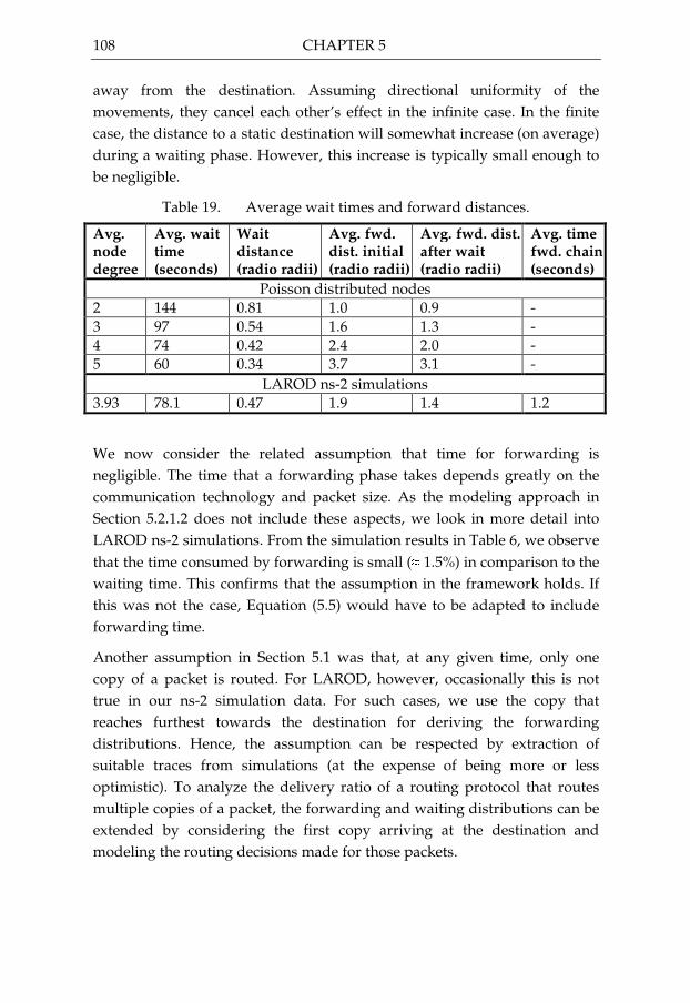
108 CHAPTER 5
away from the destination. Assuming directional uniformity of the movements, they cancel each other’s effect in the infinite case. In the finite case, the distance to a static destination will somewhat increase (on average) during a waiting phase. However, this increase is typically small enough to be negligible.
Table 19. Average wait times and forward distances.
Avg. node degree
Avg. wait time (seconds)
Wait distance (radio radii)
Avg. fwd. dist. initial (radio radii)
Avg. fwd. dist. after wait (radio radii)
Avg. time fwd. chain (seconds)
Poisson distributed nodes 2 144 0.81 1.0 0.9 - 3 97 0.54 1.6 1.3 - 4 74 0.42 2.4 2.0 - 5 60 0.34 3.7 3.1 -
LAROD ns-2 simulations 3.93 78.1 0.47 1.9 1.4 1.2
We now consider the related assumption that time for forwarding is negligible. The time that a forwarding phase takes depends greatly on the communication technology and packet size. As the modeling approach in Section 5.2.1.2 does not include these aspects, we look in more detail into LAROD ns-2 simulations. From the simulation results in Table 6, we observe that the time consumed by forwarding is small (� 1.5%) in comparison to the waiting time. This confirms that the assumption in the framework holds. If this was not the case, Equation (5.5) would have to be adapted to include forwarding time.
Another assumption in Section 5.1 was that, at any given time, only one copy of a packet is routed. For LAROD, however, occasionally this is not true in our ns-2 simulation data. For such cases, we use the copy that reaches furthest towards the destination for deriving the forwarding distributions. Hence, the assumption can be respected by extraction of suitable traces from simulations (at the expense of being more or less optimistic). To analyze the delivery ratio of a routing protocol that routes multiple copies of a packet, the forwarding and waiting distributions can be extended by considering the first copy arriving at the destination and modeling the routing decisions made for those packets.

A FRAMEWORK FOR PERFORMANCE ANALYSIS 109
ß à � � î ã � ç å � ã ä � � � ä å � ã ç å è é è ê ç ë ì í î ã ï ì ð è î ñ
In Section 5.4 we showed that the forward-wait framework can accurately match the results by simulations. This establishes some trust in the capability of the framework in predicting routing performance. In this section we illustrate how the framework can be used in connection with a large scale deployment. For the illustrations we require data for multiple node densities. Since this data is only available for the model of routing and mobility from Section 5.2.1, we will in this section use the distributions derived in Section 5.2.2. ò ó � ó õ
ö ÷ ø ù ú ÷ û ü ý þ ÿ ù � � û ÷ � ù � ÿ ù � � �A first natural use of the framework is to predict the packet delivery ratio for large scenarios. This capability is illustrated in Figure 54 and Figure 55 for the two scenarios presented in Section 5.3. The two figures show the delivery ratio for the two scenarios at a fixed node density of 4 (average node degree) for different number of nodes (100, 1000 and 10000 respectively). The impact of the increased number of nodes at a constant node density is that transmission distances increase, which is seen in the figures by the need for a longer delivery time to achieve the same delivery ratio. Due to the slightly longer distance to destination the any-to-C&C scenario has a slightly lower delivery ratio compared to the any-to-any scenario at the same packet life time.
500 1000 1500 2000 2500 3000 3500 4000 4500 50000
0.1
0.2
0.3
0.4
0.5
0.6
0.7
0.8
0.9
1
Packet life time (s)
Del
iver
y ra
tio
n=100n=1000n=10000
Figure 54. Delivery ratio for different sizes of the any-to-any scenario with
a constant average node degree.

110 CHAPTER 5
500 1000 1500 2000 2500 3000 3500 4000 4500 50000
0.1
0.2
0.3
0.4
0.5
0.6
0.7
0.8
0.9
1
Packet life time (s)
Del
iver
y ra
tio
n=100n=1000n=10000
Figure 55. Delivery ratio for different sizes of the any-to-C&C scenario
with a constant average node degree.
In a practical setting the scenario area is probably fixed, and the question that needs to be answered is the packet TTL and/or the number of radio equipped units (nodes) required to provide an acceptable delivery ratio. In Figure 56 and Figure 57 we provide the delivery ratio provided by the Forward-Wait framework for the two scenarios for different node densities at a constant area size. The area was set to 20 by 20 radio radii which means that an average node degree of 2 corresponds to an average of 255 nodes, and a node degree of 5 leads to 637 nodes. As indicated by the distributions in Section 5.2.2 a higher density means longer forwarding distances and shorter delays, which is here seen by a higher delivery ratio at a set packet time to live (TTL).

A FRAMEWORK FOR PERFORMANCE ANALYSIS 111
500 1000 1500 2000 2500 3000 3500 4000 4500 50000
0.1
0.2
0.3
0.4
0.5
0.6
0.7
0.8
0.9
1
Packet life time (s)
Del
iver
y ra
tio
c=5c=4c=3c=2
Figure 56. Delivery ratio for different node densities of the any-to-any
scenario with a constant area size.
500 1000 1500 2000 2500 3000 3500 4000 4500 50000
0.1
0.2
0.3
0.4
0.5
0.6
0.7
0.8
0.9
1
Packet life time (s)
Del
iver
y ra
tio
c=5c=4c=3c=2
Figure 57. Delivery ratio for different node densities of the any-to-C&C
scenario with a constant area size. ò ó � ó � � � � û � ÷ � � � ÷ � þ û þ � ÷ ÿ ÷ û � � � � � ÿ � ÷ � ÿ
In addition to being predictive, the framework can be used to enable a source node to dynamically set the packet TTL to achieve a desired delivery probability. To illustrate this, in Figure 58 we plot the relationship between distance to destination and TTL for various density levels with a 95% delivery probability Pd(t,d).

112 CHAPTER 5
If the TTL is fixed, Pd(t,d) can be used to determine whether a packet shall be transmitted or if a required delivery probability is set. Figure 59 shows Pd(t,d) for the mobility and routing models for an average node degree of 4. For example, if the requirement of delivery probability is 95% or higher, then the packets to destinations that are over 6.5 radio radii away can be discarded if the TTL is set to 600 seconds.
0 5 10 150
100
200
300
400
500
600
700
800
900
1000
Distance to destination (radio radii)
TT
L (s
econ
ds)
c = 2c = 3c = 4c = 5
Figure 58. TLL required for achieving 95% delivery guarantee for various
density levels.
0 5 10 150
0.1
0.2
0.3
0.4
0.5
0.6
0.7
0.8
0.9
1
Distance to destination (radio radii)
Del
iver
y pr
obab
litity
1000 s600 s400 s
Figure 59. Delivery probability in distance and TTL.

A FRAMEWORK FOR PERFORMANCE ANALYSIS 113
ß à � � è é � ä æ å é � î ì ï ã î ñ �
We have presented and validated the forward-wait mathematical framework for geographic routing. The framework describes the probability of delivery as a function of the maximum allowed delivery time and the distance to the destination. As input, the framework uses scenario- and protocol-specific random variables characterizing the forwarding and waiting phases. Combined with a description of the distance to destination, the delivery ratio can be computed for any scenario size. The framework can also be used to dynamically assess delivery probabilities based on different packet life time settings.
A major challenge in modeling routing performance is that the routing performance is scenario- and protocol-dependant. For the proposed forward-wait framework, the scenario and protocol specific elements are captured by the properties of the forwarding and waiting phases, and the distance to destination. For a specific scenario evaluated in ns-2 we determined these properties using two methods: (1) an abstract mobility model with Poisson distributed node placement and a routing protocol model, and (2) basic routing data from the ns-2 simulations. Comparing the two approaches, we observed that only with the latter input the forward-wait framework could accurately predict the routing results from the ns-2 simulations. This illustrates the difficulty of accurately describing node mobility and routing protocol using simple abstractions, and that if simplistic models are used, then the performance results are generally not reliable.
While the proposed framework is believed to be general enough to apply to other geographic routing algorithms, further work is needed to provide the evidence for this. In addition to the validation of the framework to broaden its usefulness, the prediction accuracy could be improved by explicitly considering both time and motion in the models describing forwarding and waiting.


115
6 Where We are and Where We Can Go
This chapter sums up the results of our work and reflects on future research directions. � à �
� ï ï ã î ã é æ � è é � ä � å è é �Routing in mobile ad hoc networks is challenging due to the difficulty of maintaining accurate network state in a highly dynamic environment. If complete network connectivity cannot be provided, then it becomes impossible for the nodes to maintain an up-to-date view of the network state. One way to reduce the need for system state maintenance is to use geographic routing, that is sending packets towards the destination’s position. The routing protocol is then generally state-less, but it needs to be supported by a location service that can provide the position of a destination.
In this thesis we have proposed LAROD-LoDiS, a geographic routing protocol and a location service for IC-MANETs. LAROD is a beacon-less geographic routing protocol that utilizes the store-carry-forward principle when greedy forwarding is not possible. To reduce routing delays, LAROD will start to route a packet towards the position indicated by the location service at the source node, even if this information has not been updated for a long time and is potentially incorrect. At each intermediate hop LAROD inquires the local location server if better information on the destination’s position is available, and if there is, it updates the position data in the routed packet.
To always be able to provide location data to the routing protocol in a partitioned environment the location service LoDiS uses all nodes as location servers. By using a MANET gossip technique LoDiS can distribute location data to all location servers in the system at a low overhead. The

116 CHAPTER 6
partitioned nature of the system will mean that some of the location data in a location server is somewhat inaccurate since it has not been possible to update it recently due to the absence of a contemporaneous path between location server and the destination. This information deficiency has to be addressed by the routing protocol (and it is done by LAROD). The LAROD-LoDiS combination has been shown to have a high delivery ratio with moderate delays (up to 15 minutes) in the evaluated scenarios. It is first when the clusters consist of only a couple of nodes that LAROD-LoDiS fails to provide an acceptable delivery ratio.
When studying the routing in IC-MANETs we found that how the nodes move greatly influences the routing, and for this reason we have developed a reasonably realistic mobility model that we used in our evaluations. As our main evaluation scenario, we have used a military reconnaissance mission that uses UAVs to detect enemy activities. To meet the mission objectives we have proposed the pheromone reconnaissance mobility model. By using distributed virtual pheromones the UAVs are in a robust and non-deterministic way guided to areas not recently scanned. The model has been shown to provide good search coverage, even when the communication between UAVs is poor. While we have concentrated our efforts on a UAV reconnaissance scenario, the routing results presented should be applicable to many other types of environments.
To be able to efficiently predict the routing performance of LAROD-LoDiS, and other geographic delay-tolerant routing protocols, we have created the forward-wait framework. The framework models routing as a sequence of forwarding and waiting phases. Each phase is described by a random variable that is scenario and routing protocol specific. Properties of these random variables have been established for the LAROD-LoDiS ns-2 simulations and from simpler models that intend to describe the same setting as used for the ns-2 simulations. We have shown that the forward-wait framework can accurately predict the results of simulations with properly selected random variables. The framework can be used to efficiently determine a suitable TTL and node density to achieve a minimum required delivery ratio.

WHERE WE ARE AND WHERE WE CAN GO 117
� à � í ç î ì � è î ñ
This thesis has provided a first insight into geographic routing in IC-MANETs. While we have obtained some interesting results, there are still many aspects to be explored. In this section we present some of the topics that we think warrant further study.
We have shown that LAROD-LoDiS works well in a simulated environment, but how well these results transfer to a real environment is unknown. The problems with practical tests are their costs, difficulty to repeat a test with the same conditions, and the question whether the test conditions mimic real conditions well enough. Even given these obstacles we believe that practical tests can contribute with valuable insights.
Some of the issues addressed by real-world tests could be met using high fidelity models. The model we think most important to study is the radio model. The main objective would be to determine to what extent an improved, and more computational intensive radio model impacts the routing results. Examples of radio models that could be explored are the Nakagami model [67] and log-normal shadowing [80].
As we have seen in the evaluations the node mobility greatly influences the routing result. This means that the choice of routing technology used in a specific system should be based on system connectivity properties. When developing a routing protocol it is then very important to know and describe how it is impacted by the system connectivity properties to provide systems designers with data to support their choice of routing technology. A routing protocol that is intended for general use should be evaluated in as many different system settings and environments as possible to show that it can maintain a good performance in a wide range of environments. The proposal and acceptance of a standardized test suite for ad hoc routing research would be very welcome.
LAROD builds on the principle of greedy forwarding combined with the store-carry-forward principle when forwarding is not possible. This works well as long as there are no local minima (dead ends). If there are areas where nodes never travel, then packets should be routed around these areas. Many algorithms developed to negotiate local minima for geographic routing in MANETs require that the network is fully connected. One example is the perimeter forwarding employed by GPSR [54]. We know of

118 CHAPTER 6
no attempt to solve the local minima problem for geographic routing in a DTN or an IC-MANET environment. The concept of greedily routable areas, such as in GRR [55], could be a viable approach.
In the current evaluations of LoDiS we have assumed that location information on all nodes in the system can be put into one packet. If the system grows, then at some point this assumption is no longer valid and strategies for selecting the data to transmit needs designed and evaluated. If very large systems are expected (thousands of nodes) then location information distribution will become a very interesting and delicate problem.
In this thesis we have not addressed security issues related to routing. We have assumed that all nodes in the system are benign and cooperative. This is a reasonable assumption in a closed system such as the military and in emergency services. A security mechanism that ensures that the nodes only accept data from trusted parties should be relatively simple to add provided that security credentials can be provided by a trusted element in advance of deployment. This of course assumes that the keys cannot be compromised. If keys can be compromised then we need to add a key revocation mechanism, a challenge in a disconnected system. Additional security challenges can be added depending on the assumptions regarding the system environment.
While the forward-wait framework is believed to be general enough to apply to other geographic routing algorithms, further work is needed to provide the evidence for this. In addition to an extended validation of the framework, the benefit of explicitly considering both time and motion in the models describing forwarding and waiting should be studied.
While the forward-wait framework models location service by an increased delivery distance, a more detailed description of the LoDiS location errors would be welcome. In its essence it would describe how fast information can be disseminated in an IC-MANET.
In our reconnaissance scenario we have not addressed the issue of determining a reasonable receiver of reconnaissance data. Information on nodes interested in reconnaissance data could be distributed by some kind of publish-subscribe scheme. This scheme would need to address the problems inherent in an IC-MANET, that is the delay before a subscription request is received by a information publisher or broker.

119
7 Acronyms Acronym Description
ACM Association for computing machinery AODV Ad hoc on-demand distance vector routing BGR Blind geographic routing BLR Beacon-less routing CBF Contention-based forwarding C&C Command and control cdf Cumulative distribution function CTS Clear to send DLS DREAM location service DSCP Differentiated services codepoint DSR Dynamic source routing DTN Delay-tolerant network, Disruption-tolerant network ER Epidemic routing FOPEN Foliage penetration GDBF Guaranteed delivery beacon-less forwarding GeRaF Geographic random forwarding GPS Global positioning system GPSR Greedy perimeter stateless routing GSM Global system for mobile communications HYMAD Hybrid DTN-MANET IC-MANET Intermittently connected MANET ICT Inter-contact time IEEE Institute of electrical and electronics engineers IGF Implicit geographical forwarding IP Internet protocol IPN Interplanetary network LAROD Location aware routing for delay-tolerant networks LoDiS Location dissemination service MAC Medium access MANET Mobile ad hoc network MoVe Motion vector ns-2 Network simulator version 2 OR Opportunistic routing pdf Probability density function PGR Predictive graph relay PREP Prioritized epidemic routing

120 CHAPTER 7
Acronym Description
PRoPHET Probabilistic routing protocol using history of encounters and transitivity
PSGR Priority-based geographical forwarding RFC Request for comment RTS Ready/request to send Rwp Random waypoint SLS Simple location service TRANSIMS Transportation analysis and simulation system TTL Time to live UAV Unmanned aerial vehicle UCSD University of California, San Diego URI Uniform Resource Identifier US United States
121
8 References [1] M. Abdulla, R. Simon. The Impact of the Mobility Model on Delay
Tolerant Networking Performance Analysis. Annual Simulation Symposium (ANSS). 2007. IEEE
[2] E. Altman, T. Basar, F. De Pellegrini. Optimal monotone forwarding policies in delay tolerant mobile ad-hoc networks. Performance Evaluation. Volume 67, Issue 4, 2010. Elsevier
[3] N. Aschenbruck, A. Munjal, T. Camp. Trace-based mobility modeling for multi-hop wireless networks. Computer Communications. Volume 34, Issue 6, 2011. Elsevier
[4] M. Asplund. Disconnected Discoveries: Availability Studies in Partitioned Networks. PhD Thesis. 2010. Linköping University Electronic Press. http://urn.kb.se/resolve?urn=urn:nbn:se:liu:diva-60553
[5] S. Basagni, I. Chlamtac, V. R. Syrotiuk, B. A. Woodward. A distance routing effect algorithm for mobility (DREAM). Proceedings of the ACM/IEEE International Conference on Mobile Computing and Networking (Mobicom). 1998. ACM
[6] B. Blum, T. He, S. Son, J. Stankovic. IGF: A State-Free Robust Communication Protocol for Wireless Sensor Networks. Technical Report CS-2003-11, University of Virginia. 2003
[7] T. Braun, M. Heissenbüttel, T. Roth. Performance of the Beacon-Less Routing Protocol in Realistic Scenarios. Ad Hoc Networks. Volume 8, Issue 1, 2010. Elsevier
[8] J. Broch, D. A. Maltz, D. B. Johnson, Y.-C. Hu, J. Jetcheva. A Performance Comparison of Multi-Hop wireless Ad Hoc Network Routing Protocols. Proceedings of the 4th annual ACM/IEEE international conference on Mobile computing and networking (MOBICOM). 1998. ACM
[9] R. Bruno, M. Nurchis. Survey on diversity-based routing in wireless mesh networks: Challenges and solutions. Computer Communi-cations. Volume 33, Issue 3, 2010. Elsevier

122 CHAPTER 8
[10] H. Cai, D. Y. Eun. Toward Stochastic Anatomy of Inter-meeting Time Distribution under General Mobility Models. Proceedings of the 9th ACM international symposium on Mobile ad hoc networking and computing (MobiHoc). 2008. ACM
[11] T. Camp, J. Boleng, V. Davies. A survey of mobility models for ad hoc network research. Wireless Communications and Mobile Computing. Volume 2, Issue 5, 2002. John Wiley & Son
[12] T. Camp, J. Boleng, L. Wilcox. Location Information Services in Mobile Ad Hoc Networks. Proceedings of IEEE International Conference on Communications (ICC). 2002. IEEE
[13] V. Cerf, S. Burleigh, A. Hooke, L. Torgerson, R. Durst, K. Scott, K. Fall, H. Weiss. Delay-tolerant networking architecture. RFC 4838. April 2007. RFC Editor (ftp://ftp.rfc-editor.org/in-notes/rfc4838.txt)
[14] A. Chaintreau, P. Hui, J. Crowcroft, C. Diot, R. Gass, J. Scott. Impact of Human Mobility on the Design of Opportunistic Forwarding Algorithms. Proceedings 25th IEEE International Conference on Computer Communications (INFOCOM). 2006. IEEE
[15] M. Chawala, N. Goel, K. Kalaichelvan, A. Nayak, I. Stojmenovic. Beaconless Position-based Routing with Guaranteed Delivery for Wireless Ad hoc and Sensor Networks. Acta Automatica Sinica. Volume 32, Number 6, 2006. Elsevier
[16] P.-C. Cheng, K. C. Lee, M. Gerla, J. Härri. GeoDTN+Nav: Geographic DTN Routing with Navigator Prediction for Urban Vehicular Environments. Mobile Networks and Applications. Volume 15, Number 1, 2010. Springer
[17] R. R. Choudhury. Brownian Gossip: Exploiting Node Mobility to Diffuse Information in Ad Hoc Networks. Proceedings of International Conference on Collaborative Computing: Networking, Applications and Worksharing. 2005. IEEE
[18] B. Clough. UAV Swarming? So What are Those Swarms, What are the Implications, and How do We Handle Them?. Technical report. 2004 (http://www.dtic.mil)
[19] E. M. Daly, M. Haahr. The challenges of disconnected delay-tolerant MANETs. Ad Hoc Networks. Volume 8, Issue 2, 2010. Elsevier
[20] E. M. Daly, M. Haahr. Social Network Analysis for Information Flow in Disconnected Delay-Tolerant MANETs. IEEE Transcation on Mobile Computing. Volume 8, Number 5, 2009. IEEE

REFERENCES 123
[21] S.M. Das, H. Pucha, Y.C. Hu. Performance Comparison of Scalable Location Services for Geographic Ad Hoc Routing. Proceedings IEEE 24th Annual Joint Conference of the IEEE Computer and Communications Societies (INFOCOM). 2005. IEEE
[22] M. Demmer, K. Fall. DTLSR: delay tolerant routing for developing regions. Proceedings of the 2007 workshop on Networked systems for developing regions (NSDR). 2007. ACM
[23] M. B. Donley, N. A. Schwartz. United States Air Force Unmanned Aircraft Systems Flight Plan 2009-2047. 2009. http://handle.dtic.mil/100.2/ADA505168
[24] O. Dousse, M. Franceschetti, P. Thiran. The Costly Path from Percolation to Full Connectivity. Proceedings of 42nd Annual Allerton Conference on Communication, Control and Computing. 2004. (http://www.csl.uiuc.edu/allerton/archives/allerton04/PDFs/Papers/III_A_2.pdf)
[25] O. Dousse, P.Thiran, M. Hasler. Connectivity in ad-hoc and hybrid networks. Proceedings of IEEE Twenty-First Annual Joint Conference of the IEEE Computer and Communications Societies (INFOCOM). 2002. IEEE
[26] R. Friedman, D. Gavida, L. Rodrigues, A. C. Viana, S.Voulgaris. Gossiping on MANETs: the Beauty and the Beast. Operating Systems Review. Volume 41, Issue 5, 2007. ACM
[27] H. Füßler, J. Widmer, M. Käsemann, M. Mauve, H. Hartenstein. Contention-based forwarding for mobile ad hoc networks. Ad Hoc Networks. Volume 1, Issue 4, 2003. Elsevier
[28] A. Galati, C. Greenhalgh. Human Mobility in Shopping Mall Environments. Proceedings of the Second International Workshop on Mobile Opportunistic Networking (MobiOpp). 2010. ACM
[29] P. Gaudiano, B. Shargel, E. Bonabeu, B. T. Clough. Swarm Intelligence: a New C2 Paradigm with an Application to Control of Swarms of UAVs. Proceedings of 8th ICCRTS Command and Control Research and Technology Symposium. 2003. Office of the Assistant Secretary of Defense for Networks and Information Integration
[30] N. Gazoni, V. Angelakis, V. A. Siris, R. Bruno. A Framework for Opportunistic Routing in Multi-hop Wireless Networks. Proceedings of the 7th ACM workshop on Performance evaluation of wireless ad hoc, sensor, and ubiquitous networks (PE-WASUN). 2010. ACM

124 CHAPTER 8
[31] S. Grasic, E. Davies, A. Lindgren, A. Doria. The Evolution of a DTN Routing Protocol – PRoPHETv2. In Proceedings of the 6th ACM workshop on Challenged networks (CHANTS). 2011. ACM
[32] R. Groenevelt, P. Nain, G. Koole. The message delay in mobile ad hoc networks. Performance Evaluation. Volume 62, Issues 1-4, 2005. Elsevier
[33] A. Gut. An Intermediate Course in Probability, Second Edition. ISBN 978-1-4419-0161-3. 2009. Springer
[34] S. Heimlicher, K. Salamatian. Globs in the Primordial Soup. In Proceedings of the eleventh ACM international symposium on Mobile ad hoc networking and computing (MobiHoc). 2010. ACM
[35] M. Heissenbüttel, T. Braun, T. Bernoulli, M. Wälchi. BLR: beacon-less routing algorithm for mobile ad hoc networks. Computer Communications. Volume 27, Issue 11, 2004. Elsevier
[36] M. Heissenbüttel, T. Braun, M. Wälchi, T. Bernoulli. Evaluating the Limitations of and Alternatives in Beaconing. Ad Hoc Networks. Volume 5, Issue 5, 2007. Elsevier
[37] Ó. Helgasson, S. T. Kouyoumdjieva, G. Karlsson. Does Mobility Matter? The Seventh International Conference on Wireless On-demand Network Systems and Services (WONS). 2011. IEEE
[38] T. Henderson, D. Kotz, I. Abyzov. The changing usage of mature campus-wide wireless network. Proceedings of the 10th annual international conference on Mobile computing and networking (MobiCom), 2004, ACM
[39] A. J. Hooke. Towards an Interplanetary Internet: A Proposed Strategy for Standardization. SpaceOps. 2002. SpaceOps (http://www.aiaa.org/Spaceops2002Archive/papers.html)
[40] S. Hong, I. Rhee, S. J. Kim, K. Lee, S. Chong. Routing Performance Analysis of Human-Driven Delay Tolerant Networks using the Truncated Levy Walk Model. Proceeding of the 1st ACM SIGMOBILE workshop on Mobility models (MobilityModels). 2008. ACM
[41] X. Hong, M. Gerla, G. Pei, c. Chiang. A group mobility model for as hoc wireless networks. Proceedings of the 2nd ACM international workshop on Modeling, analysis and simulation of wireless and mobile systems (MSWiM). 1999. ACM
[42] W.-J. Hsu, K. Merchant, H.-W. Shu, C.-H. Hsu, A. Helmy. Weighted Waypoint Mobility Model and its Impact on Ad Hoc Networks.
REFERENCES 125
Mobile Computing and Communications Review. Volume 9, Number 1, 2005. ACM
[43] J.-P. Hubaux, T. Gross, J.-Y. Le Boudec, M. Vetterli. Towards self-organized mobile ad hoc networks: the Terminodes project. IEEE Communications Magazine. January 2001. IEEE
[44] P. Hui, A. Chaintreau, J. Scott, R. Gass, J. Crowcroft, C. Diot. Pocket Switched Networks and Human Mobility in Conference Environments. Proceedings of the 2005 ACM SIGCOMM workshop on Delay-tolerant networking (WDTN). 2005. ACM
[45] P. Hui, J. Crowcroft, E. Yoneki. BUBBLE Rap: Social-Based Forwarding in Delay-Tolerant Networks. IEEE Transactions on Mobile Computing. Volume 10, Number 11, 2011. IEEE
[46] P. Jacquet, B. Mans, G. Rodolakis. Information Propagation Speed in Mobile and Delay Tolerant Networks. IEEE Transactions on Information Theory. 2010, Volume 56, Number 10. IEEE
[47] A. Jardosh, E. M. Belding-Royer, K. C. Almeroth, S. Suri. Towards Realistic Mobility Models for Mobile Ad Hoc Networks. Proceedings of the 9th annual international conference on Mobile computing and networking (MobiCom). 2003. ACM
[48] A. Jindal, K. Psounis. Fundamental mobility properties for realistic performance analysis of intermittently connected mobile networks. Proceedings of the Fifth Annual IEEE International Conference on Pervasive Computing and Communications Workshops (PerComW). 2007. IEEE
[49] P. Johansson, T. Larsson, N. Hedman, B. Mielczarek, M. Degermark. Scenario-based Performance Analysis of Routing Protocols for Mobile Ad-hoc Networks. Proceedings of the 5th annual ACM/IEEE international conference on Mobile computing and networking (MOBICOM). 1999. ACM
[50] D. Johnson, D. Maltz. Dynamic source routing in ad hoc wireless networks. Mobile Computing, The Springer International Series in Engineering and Computer Science, Volume 353. 1996. Springer
[51] D. Johnson, Y. Hu, D. Maltz. The Dynamic Source Routing Protocol (DSR) for Mobile Ad Hoc Networks for IPv4. RFC 4728. February 2007. RFC Editor (ftp://ftp.rfc-editor.org/in-notes/rfc4728.txt)
[52] P. Juang, H. Oki, Y. Wang, M. Martonosi, L.S. Peh, D. Rubenstein. Energy-efficient computing for wildlife tracking: design tradeoffs and early experiences with ZebraNet. Proceedings of the 10th international

126 CHAPTER 8
conference on Architectural support for programming languages and operating systems (ASPLOS-X). 2002. ACM
[53] T. Karagiannis, J.-Y. Le Boudec, M. Vojnovic. Power Law and Exponential Decay of Inter Contact Times between Mobile Devices. Proceedings of the 13th annual ACM international conference on Mobile computing and networking (MobiCom). 2007. ACM
[54] B. Karp, H.T. Kung. GPSR: Greedy perimeter stateless routing for wireless networks. Proceedings of the 6th annual international conference on Mobile computing and networking (MobiCom). 2000. ACM
[55] A-M. Kermarrec, G. Tan. Greedy Geographic Routing in Large-Scale Sensor Networks: A Minimum Network Decomposition Approach. Proceedings of the eleventh ACM international symposium on Mobile ad hoc networking and computing (MobiHoc). 2010. ACM
[56] M. Kim, D. Kotz, S. Kim. Extracting a mobility model from real user traces. Proceedings of 25th IEEE International Conference on Computer Communications (INFOCOM). 2006. IEEE
[57] R. Krishnan. REDTIP: Retrofitting Disruption-Tolernace into the Internet Protocol. Military Communications Conference (MILCOM). 2009. IEEE
[58] J. Kurhinen, J. Janatuinen. Delay Tolerant Routing in Sparse Vehicular Ad Hoc Networks. Acta Electrotechnica et Informatica. Volume 8, Number 3, 2008, Versita
[59] J.-Y. Le Boudec, M. Vojnovi . Perfect Simulation and Stationarity of a Class of Mobility Models. Proceedings of 24th Annual Joint Conference of the IEEE Computer and Communications Societies (INFOCOM). 2005. IEEE
[60] J. LeBrun, C. Chuah, D. Ghosal, M. Zhang. Knowledge-Based Opportunistic Forwarding in Vehicular Wireless Ad Hoc Networks. Proceedings of IEEE 61st Vehicular Technology Conference (VTC). 2005. IEEE
[61] I. Leontiadis, C. Mascolo. GeOpps: Geographical Opportunistic Routing for Vehicular Networks. Proceedings of IEEE International Symposium on a World of Wireless, Mobile and Multimedia Networks (WoWMoM). 2007. IEEE
[62] A. Lindgren, A. Doria, O. Schelén. Probabilistic Routing in Intermittently Connected Networks. Lecture notes in computer science, volume 3126. 2004. Springer

REFERENCES 127
[63] G. Marfia, G. Pau, E. De Sena, E. Giordano, M. Gerla. Evaluating Vehicle Network Strategies for Downtown Portland: Opportunistic Infrastructure and the Importance of Realistic Mobility Models. Proceedings of the 1st international MobiSys workshop on Mobile opportunistic networking (MobiOpp). 2007. ACM
[64] M. McNett, G.M. Voelker. Access and mobility of wireless PDA users. Technical report, Computer Scinece and Engineering, UC San Diego. 2004
[65] R. Meester, R. Roy. Continuum percolation. 1996. Cambridge University Press
[66] P. Nain, D. Towsley, B. Liu, Z. Liu. Properties of Random Direction Models. Proceedings of 24th Annual Joint Conference of the IEEE Computer and Communications Societies (INFOCOM). 2005. IEEE
[67] M. Nakagami. The m-distribution, a General Formula of Intensity Distribution of the Rapid Fading. Statistical Methods in Radio Wave Propagation (editor W. G. Hoffman). 1960. Pergamon Press
[68] V. Naumov, R. Baumann, T. Gross. An Evaluation of Inter-Vehicle Ad Hoc Networks Based on Realistic Vehicular Traces. Proceedings of the 7th ACM international symposium on Mobile ad hoc networking and computing (MobiHoc). 2006. ACM
[69] W. Navidi, T. Camp. Stationary Distributions for the Random Waypoint Mobility Model. IEEE Transactions on Mobile Computing. Volume 3, Number 1, 2004. IEEE
[70] http://nsnam.isi.edu/nsnam/index.php/Main_Page [71] D. Pack, G. Dudevoir, P. Lima, S. Gruber. Negotiating between
Communication and Cooperation for Multiple Unmanned Aerial Vehicles. Military Communications Conference (MILCOM). 2009. IEEE
[72] C. Papageorgiou, K. Birkos, T. Dagiuklas, S. Kotsopoulos. Modeling human mobility in obstacle-constrained ad hoc networks. Ad Hoc networks. Volume 10, Issue 3, 2012. Elsevier
[73] A. Papoulis. Probability, Random Variables, and Stochastic Processes. 1991. McGraw-Hill
[74] H. V. D. Parunak, S. A. Brueckner, J. J. Odell. Swarming Coordination of Multiple UAV’s for Collaborative Sensing. Proceedings of 2nd AIAA Unmanned Unlimited Systems Technologies and Operations Aerospace land and Sea Conference and Workshop & Exhibit. 2003. American Institute of Aeronautics and Astronautics

128 CHAPTER 8
[75] M. Pascoe-Chalke, J. Gomez, V. Rangel, M. Lopez-Guerrero. Route duration modeling for mobile ad-hoc networks. Wireless Networks. Volume 16, Number 3, 2010. Springer
[76] A. Pentland, R. Fletcher, A. Hasson. DakNet: rethinking connectivity in developing nations. Computer. Volume 37 , Issue 1, 2004. IEEE
[77] C. Perkins, E. Belding-Royer, S. Das. Ad hoc On-Demand Distance Vector (AODV) Routing. RFC 3561. July 2003. RFC Editor (ftp://ftp.rfc-editor.org/in-notes/rfc3561.txt)
[78] J. Quintanilla, S. Torquato, R. M. Ziff. Efficient measurement of the percolation threshold for fully penetrable discs. Journal of Physics A: Mathematical and General. Volume 22, Number 4, 2000. IOPscience
[79] R. Ramanathan, R. Hansen, P. Basu, R. Rosales-Hain, R. Krishnan. Prioritized Epidemic Routing for Opportunistic Networks. Proceedings of the 1st international MobiSys workshop on Mobile opportunistic networking (MobiOpp). 2007. ACM
[80] T.S. Rappaport. Wireless Communications, 2nd edition. 2002. Prentice Hall
[81] G. Resta, P. Santi. A Framework for Routing Performance Analysis in Delay Tolerant Networks with Application to Noncooperative Networks. IEEE Transactions on Parallel and Distributed Systems. Volume 23, Issue 1, 2012. IEEE
[82] I. Rhee, M. Shin, S. Hong, K. Lee, S. Chong. On the Levy-walk Nature of Human Mobility. Proceedings of the 27th Conference on Computer Communications (INFOCOM). 2008. IEEE
[83] R.R. Roy. Handbook of Mobile Ad Hoc Networks for Mobility Models. 2011. Springer
[84] E.M. Royer, P.M. Melliar-Smith, L. E. Moser. An analysis of the optimum node density for ad hoc mobile networks. Proceedings of IEEE International Conference on Communications (ICC). 2001. IEEE
[85] M. Saleem, S.A. Khayam, M. Farooq. On Performance Modeling of Ad Hoc Routing Protocols. EURASIP Journal on Wireless Communications and Networking. 2010. Hindawi
[86] G. Sandulescu, S. Nadjm-Tehrani. Adding Redundancy to Replication in Window-aware Delay-tolerant Routing. Journal of Communications. Volume 5, Number 2, 2010. Academy Publisher
[87] J. A. Sauter, R. Matthews, H. V. D. Parunak, S. A. Brueckner. Performance of Digital Pheromones for Swarming Vehicle Control.

REFERENCES 129
Proceedings of the fourth international joint conference on Autonomous agents and multiagent systems (AAMAS). 2005. ACM
[88] A. Scherrer, P. Borgnat, E. Fleury, J.-L. Guillaume, C. Robardet. Description and simulation of dynamic mobility networks. Computer Networks. Volume 52, Issue 15, 2008, Elsevier
[89] M. Schwamborn, N. Aschenbruck, P. Martini. A Realistic Trace-based Mobility Model for First Responder Scenarios. Proceedings of the ACM-IEEE International Symposium on Modeling, Analysis and Simulation of Wireless and Mobile Systems (MSWIM). 2010. ACM
[90] T. Small, Z. J. Haas. The Shared Wireless Infostation Model - A New Ad Hoc Networking Paradigm (or Where there is a Whale, there is a Way). Proceedings of the 4th ACM international symposium on Mobile ad hoc networking & computing (MobiHoc). 2003. ACM
[91] V.N.G.J. Soares, J.J.P.C. Rodriges, F. Farahmand. GeoSpray: A geographic routing protocol for vehicular delay-tolerant networks. Information Fusion. Article in press. Elsevier
[92] L. Song, D.F. Kotz. Evaluating Opportunistic Routing Protocols with large Realistic Contact Traces. Proceedings of the second workshop on Challenged networks (CHANTS). 2007. ACM
[93] Specification of the Bluetooth system Version 2.1 + EDR, 26 July 2007, Bluetooth SIG, available from http://bluetooth.com/Bluetooth/Learn/Technology/Specifications/
[94] T. Spyropoulos, K. Psounis, C.S. Raghavendra. Efficient Routing in Intermittently Connected Mobile Networks: The Single-Copy Case. IEEE/ACM Transactions on Networking. Volume 16, Number 1, 2008. IEEE/ACM
[95] T. Spyropoulos, K. Psounis, C.S. Raghavendra. Efficient Routing in Intermittently Connected Mobile Networks: The Multiple-Copy Case. IEEE/ACM Transactions on Networking. Volume 16, Number 1, 2008. IEEE/ACM
[96] T. Spyropoulos, K. Psounis, C.S. Raghavendra. Performance Analysis of Mobility-assisted Routing. Proceedings of the 7th ACM international symposium on Mobile ad hoc networking and computing (MobiHoc). 2006. ACM
[97] T. Spyropoulos, K. Psounis, C.S. Raghavendra. Spray and wait: an efficient routing scheme for intermittently connected mobile networks. Proceedings of the 2005 ACM SIGCOMM workshop on Delay-tolerant networking (WDTN). 2005. ACM

130 CHAPTER 8
[98] T. Spyropoulos, T. Turletti, K. Obraczka. Utility-based Message Replication for Intermittently Connected Heterogeneous Networks. Proceedings of IEEE International Symposium on a World of Wireless, Mobile and Multimedia Networks (WoWMoM). 2007. IEEE
[99] J. Su, A. Goel, E. de Lara. An Empirical Evaluation of the Student-Net Delay Tolerant Network. Proceedings of Third Annual International Conference on Mobile and Ubiquitous Systems: Networking & Services (MobiQuitous). 2006. IEEE
[100] V. Tolety. Load Reduction in Ad Hoc Networks Using Mobile Servers. Master’s thesis. 1999. Colorado School of Mines
[101] TRANSIMS. The Travel Model Improvement Program. http://tmip.fhwa.dot.gov/community/user_groups/transims
[102] A. Vahdat, D. Becker. Epidemic Routing for Partially-Connected Ad Hoc Networks. Tech. Rep. CS-2000-06, Duke University. 2000
[103] P. Vincent, I. Rubin. A framework and analysis for cooperative search using UAV swarms. Proceedings of the 2004 ACM symposium on Applied computing. 2004. ACM
[104] J. Whitbeck, M.D. de Amorim, V. Conan, M. Ammar, E. Zegura. From encounters to plausible mobility. Pervasive and Mobile Computing. Volume 7, Issue 2, 2011. Elsevier
[105] J. Whitbeck, V. Conan. HYMAD: Hybrid DTN-MANET routing for dense and highly dynamic wireless networks. Computer Communications. Volume 33, Issue 13, 2010. Elsevier
[106] M. Witt, V. Turau. Robust and low-communication geographic routing for wireless ad hoc networks. Wireless Communications and Mobile Computing. Volume 10, Issue 4, 2010. Wiley
[107] Y. Xu, W.-C. Lee, J. Xu, G. Mitchell. PSGR: Priority-based Stateless Geo-Routing in Wireless Sensor Networks. Proceedings of IEEE International Conference on Mobile Adhoc and Sensor Systems (MASS). 2005. IEEE
[108] C. Zhang. Routing in Intermittently Connected Mobile Ad Hoc Networks and Delay tolerant networks: Overview and Challenges. IEEE Communications Surveys & Tutorials. Volume 8, Issue 1, 2006. IEEE
[109] X. Zhang, J. Kurose, N. Levine, D. Towsley, H. Zhang. Study of a Bus-based Distruption-Tolerant Network: Mobility Modeling and Impact on Routing. Proceedings of the 13th annual ACM international

REFERENCES 131
conference on Mobile computing and networking (MobiCom). 2007. ACM
[110] X. Zhang, G. Neglia, J. Kurose, D. Towsley. Performance modeling of epidemic routing. Computer Networks. Volume 51, Issue 10, 2007. Elsevier
[111] B. Zhou, K. Xu, M. Gerla. Group and Swarm Mobility Models for Ad Hoc Network Scenarios Using Virtual Tracks. Military Communications Conference (MILCOM). 2004. IEEE
[112] ZigBee Specification, 1 December 2006, ZigBee Standards Organization
[113] M. Zorzi, R.R. Rao. Geographic Random Forwarding (GeRaF) for Ad Hoc and Sensor Networks: Energy and Latency Performance. IEEE Transactions on Mobile Computing. Volume 2, Number 4, 2003. IEEE
[114] M. Zorzi, R.R. Rao. Geographic Random Forwarding (GeRaF) for Ad Hoc and Sensor Networks: Multihop Performance. IEEE Transactions on Mobile Computing. Volume 2, Number 4, 2003. IEEE


133
! " " # $ % & ' () # * + , - . / & , $ 0 1 # , * 2 3 # / * & + 4In percolation theory there are some different ways to describe the critical density at which the system percolates. In this appendix we will give an overview of how these densities relate to each other for the two-dimensional case with a constant radius.
Percolation theory normally studies when areas intersects, which for circular areas means when the center points are within two radii of each other. In ad hoc networks we are instead interested in when two nodes are within each others radio range. This difference means that the natural way to describe the percolation threshold differs somewhat in these two research fields. For example, the average node degree is four times greater than the filling factor used in continuum percolation theory since the filling factor is computed based on when the circles of two nodes intersect and the node degree is based on when nodes are within communication range of each other.
The table below summarizes the most common parameters in percolation and ad hoc network research, and how they relate to each other. From these relationships we can derive the average node degree, c, from the volume fraction, 5 , assuming that 5 has been derived using the unit disc radius for intersection analysis (R=1) to )1ln(4 ϕ−−=c .
Table 20. Percolation theory and ad hoc network parameters, and their relationships.
Parameter Description Relationship
R Radius of discs for intersection analysis.
r Nominal radio range. r = 2R 6 Poisson process density. 7 Node density. Equals to the Poisson process
density for Poisson distributed nodes. 5 Volume fraction. Fraction of
the area covered by discs. For Poisson distributed nodes: 1-e-
8 9R ([65], Definition 5.1)
c Average node degree. : ; r²


135
! " " # $ % & ' <= > ? @ A > A B C D B E F ? G H I H B J K H D C D B B L M NTo be able to use Spray and Wait [95][97] as a comparative baseline to LAROD we needed a Spray and Wait implementation in ns-2. Spray and Wait was originally evaluated using a custom event-driven simulator with a slotted MAC protocol. An existing implementation of Spray and Wait for ns-2 by Abdulla and Simon [1] has been consulted and found to have some deficiencies (reliable transfers are assumed, a node only uses local knowledge in the sending node to determine if a packet shall be sprayed at an encounter, and when receiving a sprayed packet for a second time a node silently drops it and the total number of sprayed copies is reduced). We have therefore implemented a move faithful implementation of the algorithm in ns-2. To clarify some implementation details we have been in contact with the first author of Spray and Wait, and we have received the following clarifications.
• In the original simulations it was assumed that the MAC layer performed beaconing to advertise a node’s presence.
• At each encounter the nodes exchange information on held messages in order to know which packets to exchange.
When implementing Spray and Wait in ns-2 with IEEE 802.11 as MAC layer a number of implementation choices had to be made for issues that were abstracted away in the original implementation. We have generally preferred a simpler solution over a complex one when possible, without sacrificing the protocol’s performance. This has led us to keep as little state in the nodes as possible, and let events initiate actions. An example is the decision not to maintain a neighborhood list. The main design choices and their rationale are presented in Table 21.

136 APPENDIX 2
Table 21. Spray and Wait implementation choices and rationale.
Choice Motivation
Each node regularly sends a beacon. Needed to determine when a node is in the neighborhood.
Message transfers are initiated when a node hears a beacon.
Simplifies protocol design, and improves the probability that the node will still be in the neighborhood when a message is transmitted.
After receiving a beacon there is a reserved time (the Query phase) for exchanging information on data messages to transfer.
Needed to increase the probability that the queries and responses are not delayed due to congestion.
Messages are only transferred to the node sending the beacon.
Simplifies protocol design. A node receiving the beacon will soon emit its own beacon and then messages will be transmitted to it.
Each node maintains information regarding the nodes that it knows currently hold copies of messages that it holds.
Needed to reduce the amount of data exchanged in the Query phase.
Figure 60. Packet exchange
beaconing node
querying node
beacon
query
response
message 1
ack 1
message 2
ack 2
Query phase
Message transmission
phase

IMPLEMENTING SPRAY AND WAIT IN NS-2 137
The overall scheme for the implementation of Spray and Wait in ns-2 is illustrated in Figure 60, which describes the packet and message exchange sequence. A node receiving a beacon packet responds with a query packet if it has some data messages the beaconing node might be interested in. A query can contain up to 100 message ids. As a response to a query packet the beaconing node replies with a query response packet detailing the data messages it is interested in. For the other data messages the beaconing node details why it did not request it. The reply can either be that it already has the message or that the message has been received by the destination.
To limit contention that might delay the transfer of a query packet, and its response packet, no data messages may be sent to the beaconing node for some set time after a beacon was received (in our simulations we have used 0.15 seconds). Additionally the query is randomly delayed for some time after the beacon is received (we have used up to 0.10 seconds). Except for this, the MAC layer is responsible for handling contention and the routing agent sends messages to the MAC layer whenever it has something to send.
After the query phase, the nodes having data messages to send to the beaconing node start to transmit these. When the beaconing node has received a message it responds with an acknowledgement to tell the querying node that the message was received.
On a wireless medium transmissions can fail due to interference or other factors and even with relatively reliable MAC layers such as IEEE 802.11 packets might be lost. The impact of lost messages for our implementation of Spray and Wait is detailed in Table 22. The only loss whose impact is worse than a delay in the spreading of messages is the loss of an ack packet. When an ack packet is lost then more copies of a packet will be distributed in the network than what was intended, which results in higher (and unnecessary) resource utilization.

138 APPENDIX 2
Table 22. Impact of lost packets on Spray and Wait.
Packet type Impact
Beacon, Query or Response packet
No messages can be exchanged. New message exchange possibility when the next beacon is transmitted.
Message packet The message was not exchanged. New message exchange possibility when the next beacon is transmitted.
Ack packet The querying node does not know that the message was received by the beaconing node, and it will keep the copies that are now taken by the beaconing node. This means that extra copies of messages are injected into the network unnecessarily.
We believe that the proposed realization of Spray and Wait is a fair realization of the original design in a full packet level implementation. We have put considerable effort into making the design as efficient as reasonably possible to keep the previously presented attractive properties of Spray and Wait. O P Q R S T U V W V X Y Z V [ \ ] V U V ^ _ \ _ U `For an implementation of Spray and Wait the two parameters L (number of spray copies), and beacon interval, have to be determined. Intuitively the higher L is set the better the delivery ratio should become, but at a higher overhead. A shorter beacon interval will definitely increase the overhead, and a too long beacon interval will probably reduce the delivery ratio due to missed communication opportunities. There is probably some beacon rate where the delivery ratio will no longer go up with an increased beacon rate.
The optimal Spray and Wait parameters depend on the network properties. For the determination of the parameters in this section we have used the evaluation scenario for LAROD-LoDiS. The main parameters are summarized in Table 23.

IMPLEMENTING SPRAY AND WAIT IN NS-2 139
Table 23. Scenario parameters
Scenario name Parameter Reconnaissance Slow Rwp Fast Rwp
Mobility model Pheromone reconnaissance
Random waypoint
Random waypoint
Simulation area 2000x2000 meters
2000x2000 meters
2000x2000 meters
Number of nodes 80 80 80 Radio range 250 meters 250 meters 250 meters Node speed 1.4 m/s 1.4 m/s 1.0-10.0 m/s Node pause time - 0.0 seconds 0.0 seconds
Establishing the best number of spray copies (L) has not been trivial. For the slow random waypoint and the reconnaissance scenario, the packet delivery ratio clearly increases with an increased L. The cost of increasing L for the overhead is also noticeable. When different values of L were examined with the fast random waypoint scenario, then the overhead was substantially higher compared to the slow random waypoint scenario. The reason that we get an increase in effort for higher speeds is that during a transfer of a set of data messages the nodes move out of each other’s transmission range, and the sending node tries to transfer messages to a node that cannot receive them. Avoiding such partial transmissions needs a specific mechanism to take account of the contact window, which is not available in Spray and Wait [86]. The studies we made clearly indicate that L is a scenario dependant parameter. We have chosen to use L = 10 and 20 as described in Table 24. These choices are not far from the choice of L (10 and 16) in the original evaluation of Spray and Wait.
The delivery ratio does go down with an increased beacon interval, but the relationship is not that strong. The relationship is somewhat stronger for the fast random waypoint scenario. The overhead is definitely impacted by the beacon interval, and an interval shorter than 20 seconds is not recommended. To improve comparability with LAROD-LoDiS we have chosen the LoDiS broadcast interval of 40 seconds for the Spray and Wait beacon interval, see Table 24.
Table 24. Spray and Wait parameters.
Reconnaissance Slow Rwp Fast Rwp
L 10, 20 20 10 Beacon interval 40 seconds 40 seconds 40 seconds


141
a ? ? A B J D b cd e > ? @ A b D C I e f g A G D h D B E C i Aj k l m n k o p m k q r q s t q n u v n w k r x j k l m v r y zIn illustrating the complexity of determining forwarding distance analytically, it is instructive to make a couple of major simplifications. First, we assume that the nodes are Poisson distributed, and secondly, that the destination is infinitely far away. With these assumptions, the progress forwarding area has a constant shape. Yet, an analytical derivation of the forwarding distance is still practically unfeasible. For the first hop from the source, it is trivial to establish whether or not a packet can be forwarded, and the probability distribution of the progress if forwarding takes place. For the possible second hop, the distribution becomes harder to derive. Depending on the location of the custodian after the first hop, there are three different cases, as illustrated in Figure 61. Under the assumption of perfect custodian selection, the intersection of the two forwarding areas does not contain any other node. Although the process is cumbersome, it is feasible to derive analytical expressions on a case-by-case basis. However, with a chain of forwarding operations, the derivation becomes overwhelmingly complex and practically unfeasible. This justifies the use of Monte Carlo simulations to determine the distributions of the forwarding phase.
(a) (b) (c)
Figure 61. An illustration of the custodian location after first hop.


143
{ | | z r w k } ~� v r w q � � v n k v o � z lIn this appendix we will provide a short introduction to continuous random variables and their properties. A more full and rigid description of random variables can be found in a standard probability theory text book such as An Intermediate Course in Probability by Allan Gut [33].
A random variable describes an event with an unknown outcome. While the outcome is unknown, the probability of a specific outcome might be known. We use the notation P(expression) to describe the probability that the expression is true. A commonly used, and convenient, description of a random variable is the cumulative distribution function (cdf). The cdf of the random variable X is the probability that it will have the value x or lower, and it is defined in Equation (2.5). A related property is the probability density function (pdf) which is the derivative of the cdf for all points where the cdf is continuous, and it is defined in Equation (2.6)4. From their definitions the cdf is an increasing function that goes from 0 to 1, and the pdf is always positive or zero.
)(),( xXPxXcdf ≤= -� <x<� (2.5) �∞−
=x
dyyXpdfxXcdf ),(),( -� <x<� (2.6)
Random variables can be used in mathematical expressions where the result is a new random variable. The pdf of a sum of two independent random variables is according to Equation (2.7), and if a random variable is transformed by a strictly monotone function y=g(x) where its inverse exists, x=g-1(y), then the resulting pdf is according to Equation (2.8). � �∞
∞−
∞
∞−
−+⋅⋅=+ dxdyzyxyYpdfxXpdfzYXpdf ))((),(),(),( δ (2.7)
( ) )())(,(),( 11 ygdy
dygXpdfyXgpdf −− ⋅= (2.8)
4 In statistics cdf(X, x) is often denoted FX(x) and pdf(X, x) fX(x).


145
{ | | z r w k } �j k l m v r y z j k l m n k o p m k q r l � z m u z z r � v k n lq s � q w z lIn this appendix we derive the distance distribution for the two scenarios described in section 5.3. In the derivation of the density function we make use of the relationships below. � �
−+⋅⋅=+ dxdytyxyBpdfxApdftBApdf ))((),(),(),( δ � �−−⋅⋅=− dxdytyxyBpdfxApdftBApdf ))((),(),(),( δ
dy
dxxXpdfyXfpdf ⋅= ),()),(( , where f(x) is a continuous and strictly
increasing or decreasing function of x in the range where pdf(X,x) > 0. � � � � � � � � � � � � � � � � � � � � � � � � � � � � � � � � � � � �� � � � � � � ¡ ¢ £ � � � � � � � � � � ¤ ¥ � ¤ � �In this section we derive the source-destination distance density function for two uniformly distributed nodes within a square area. Let the positions of the two nodes A and B be represented by random variables defined below, where k is the side length of the square.
A = (XA, YA)
B = (XB, YB) ¦§¨ ≤≤====
otherwise0
0/1),(),(),(),(
kxkxYpdfxXpdfxYpdfxXpdf BBAA
The random variable representing the distance between the two nodes has then the following expression.
( ) ( )22BABA YYXXBAD −+−=−=
The density function of D, pdf(D,d), can then be derived as follows.

146 APPENDIX 5
©ª©«¬ ≤<−≤≤+
=
=©©©©©©©©®¯©©©©ª©©
©©«¬≤<⋅
≤≤⋅
=
=−−⋅⋅=−=−° ° ° °+
otherwise0
0//1
0//1
otherwise0
011
011
))((),(),(),(),(
2
2
0
kdkdk
d-kkdk
kddxkk
d-kdxkk
dxdydyxyXpdfxXpdfdYYpdfdXXpdf
k
d
dk
BABABA δ
±²³ ≤≤−=−otherwise0
0/2/2),(
2 kdkdkdXXpdf BA
( ) ( ) ( )
´́µ́́¶· ≤≤−=
=⋅−=−=−
otherwise0
011
2
1,,,)(
22
22
kdkdk
ddXXpdfdXXpdfdXXpdf BABABA

DISTANCE DISTRIBUTIONS BETWEEN PAIRS OF NODES 147
( ) ( )( ) ( )( ) ( )( )
¸̧̧̧¹̧̧¸̧º»
<<−−+−¼¼½¾¿¿ÀÁ−
−
≤≤+−
=
=ÂÂÂÂÂÃÂÂÂÂÂÄÅÂÂÂÂÂÆ
ÂÂÂÂÂÇÈ<<ÉÉÊËÌÌÍÎ +−−+ÏÏÐÑÒÒÓÁ
−
≤≤ÉÉÊËÌÌÍÎ +−−
+ÏÏÐÑÒÒÓÁ−
=
=ÂÂÂÂÃÂÂÂÂÄÅÂÂÂÂÆÂÂ
ÂÂÇÈ<<ÏÏÐÑÒÒÓÁ −ÏÏÐÑÒÒÓÁ −
≤≤ÏÏÐÑÒÒÓÁ −ÏÏÐÑÒÒÓÁ −
=
=−+⋅−⋅−=−+−
−
−
−
−
−
ÔÔ Ô Ô
otherwise0
242
2
2tan
2
04
otherwise0
222
tan2
022
tan2
otherwise0
21111
01111
))((,,,
2243
2
22
21
2
2432
22433
12
2
0
4331
2
2222
2
022
2222
2
2
2
2
kdkk
d
k
kd
kkdk
dk
k
kdk
d
k
d
k
kdkk
x
k
x
k
xd
xd
x
k
kdk
x
k
x
k
xd
xd
x
k
kdkdxkd-xkkxk
kddxkd-xkkxk
dxdydyxyYYpdfxXXpdfdYYXXpdf
k
kd
d
k
kd
d
BABABABA
π
δ
( ) ( )( )
ÕÕÕÕÖÕÕÕÕ×Ø
<<ÙÙÚÛÜÜÝÞ −−+−ÙÙÚÛÜÜÝÞ−
−⋅
≤≤ÙÙÚÛÜÜÝÞ +−⋅
=
=⋅−+−=
−
otherwise0
242
2
2tan
22
04
2
2,),(
4
2
3
22
222
221
2
4
2
32
222
kdkk
d
k
kd
kkdk
dk
kd
kdk
d
k
d
kd
ddYYXXpdfdDpdf BABA
π
ß à á â ã ä å æ ç è é ê ã ä å æ ë ä ì í æ ä î è ï ê æ ð ê ê è çñ è ä ò î ë ó ô õ ã ä å æ ë ä ì í æ ê ö ÷ î ö ê ç è ö ç ø æ ç æ ä é÷ î ö êIn this section we derive the source-destination distance density function between a uniformly distributed node within a square area and a node

148 APPENDIX 5
located at the center of one of the square edges. Let the positions of the two nodes A and B be represented as defined below, where k is the side length of the square.
A = (XA, YA)
B = (k/2, 0) ùúû ≤≤==
otherwise0
0/1),(),(
kxkxYpdfxXpdf AA
The random variable representing the distance between the two nodes has then the following expression.
( ) ( )222/ AA YkXBAD +−=−=
The density function of D, pdf(D,d), can then be derived as follows. üýþ ≤≤−=−
otherwise
kdkkdkXpdf A 0
2/2//1),2/( ÿ�� ≤≤
=−otherwise
kdkdkXpdf A 0
2/0/2),2/(
( )( ) ( )
( ) ������� ≤≤=⋅−=
=−=−
otherwise
kddk
ddkXpdf
dkXpdfdkXpdf
A
AA
0
4/01
2
1,2/
,2/,2/
2
22
),(),( dYpdfdYpdf AA =
( )( ) ( ) ������ ≤≤=⋅=
otherwise
kddk
ddYpdfdYpdf AA
0
02
1
2
1,,
2
2

DISTANCE DISTRIBUTIONS BETWEEN PAIRS OF NODES 149
( ) ( )( ) ( )( ) ( )( ) ( )( )
��
<<�������� �������� −⋅−��������−
⋅
≤<��������−
⋅
≤≤
=
=
���
��
<<�������� ��������−
⋅
≤<�������� ��������−
⋅
≤≤�������� ��������−
⋅
=
=���
��
<<−
≤<−
≤≤−
=
=−+⋅⋅−=+−
−−
−
−
−
−
−
−
��� � �
otherwise
kdkk
k
kd
kd
k
kdk
kkd
k
kd
k
otherwise
kdkk
xd
x
kdk
kxd
x
kdk
xd
x
otherwise
kdkdx
xdkxk
kdk
dxxdkxk
kddx
xdkxk
dxdydyxyYpdfxkXpdfdYkXpdf
k
kd
k
d
k
kd
k
d
AAAA
0
4
5tan2
4/
2/tan2
44/
2/tan2
40
0
4
5tan2
4tan2
40tan2
0
4
5
2
11
42
11
40
2
11
,,2/,2/
222
21
2
1
22
2
2
1
2
2
22
4/
21
22
4/
0
21
2
0
21
22
4/
224/
0
2
0
2222
2
2
2
2
2
2
π
δ

150 APPENDIX 5
( ) ( )( )
��������������� !
<<""#$%%&' ""#$%%&' −⋅−""#$%%&'−
⋅
≤<""#$%%&'−
⋅
≤≤
=
=⋅+−=
−−
−
otherwise
kdk
k
kd
kd
k
k
d
kdk
kd
k
k
d
kd
k
d
ddYkXpdfdDpdf AA
0
4
5tan2
4tan
4
44tan
4
20
2
2,2/),(
22
221
22
1
2
22
22
1
2
2
222
π

Department of Computer and Information Science
Linköpings universitet
Dissertations
Linköping Studies in Science and Technology
Linköping Studies in Arts and Science Linköping Studies in Statistics
Linköpings Studies in Informatics
Linköping Studies in Science and Technology
No 14 Anders Haraldsson: A Program Manipulation
System Based on Partial Evaluation, 1977, ISBN 91-
7372-144-1.
No 17 Bengt Magnhagen: Probability Based Verification
of Time Margins in Digital Designs, 1977, ISBN 91-
7372-157-3.
No 18 Mats Cedwall: Semantisk analys av process-
beskrivningar i naturligt språk, 1977, ISBN 91- 7372-
168-9.
No 22 Jaak Urmi: A Machine Independent LISP Compiler
and its Implications for Ideal Hardware, 1978, ISBN
91-7372-188-3.
No 33 Tore Risch: Compilation of Multiple File Queries in
a Meta-Database System 1978, ISBN 91- 7372-232-4.
No 51 Erland Jungert: Synthesizing Database Structures
from a User Oriented Data Model, 1980, ISBN 91-
7372-387-8.
No 54 Sture Hägglund: Contributions to the Development
of Methods and Tools for Interactive Design of
Applications Software, 1980, ISBN 91-7372-404-1.
No 55 Pär Emanuelson: Performance Enhancement in a
Well-Structured Pattern Matcher through Partial
Evaluation, 1980, ISBN 91-7372-403-3.
No 58 Bengt Johnsson, Bertil Andersson: The Human-
Computer Interface in Commercial Systems, 1981,
ISBN 91-7372-414-9.
No 69 H. Jan Komorowski: A Specification of an Abstract
Prolog Machine and its Application to Partial
Evaluation, 1981, ISBN 91-7372-479-3.
No 71 René Reboh: Knowledge Engineering Techniques
and Tools for Expert Systems, 1981, ISBN 91-7372-
489-0.
No 77 Östen Oskarsson: Mechanisms of Modifiability in
large Software Systems, 1982, ISBN 91- 7372-527-7.
No 94 Hans Lunell: Code Generator Writing Systems, 1983,
ISBN 91-7372-652-4.
No 97 Andrzej Lingas: Ad vances in Minimum Weight
Triangulation, 1983, ISBN 91-7372-660-5.
No 109 Peter Fritzson: Towards a Distributed Programming
Environment based on Incremental Compilation,
1984, ISBN 91-7372-801-2.
No 111 Erik Tengvald: The Design of Expert Planning
Systems. An Experimental Operations Planning
System for Turning, 1984, ISBN 91-7372- 805-5.
No 155 Christos Levcopoulos: Heuristics for Minimum
Decompositions of Polygons, 1987, ISBN 91-7870-
133-3.
No 165 James W. Goodwin: A Theory and System for Non-
Monotonic Reasoning, 1987, ISBN 91-7870-183-X.
No 170 Zebo Peng: A Formal Methodology for Automated
Synthesis of VLSI Systems, 1987, ISBN 91-7870-225-9.
No 174 Johan Fagerström: A Parad igm and System for
Design of Distributed Systems, 1988, ISBN 91-7870-
301-8.
No 192 Dimiter Driankov: Towards a Many Valued Logic of
Quantified Belief, 1988, ISBN 91-7870-374-3.
No 213 Lin Padgham: Non-Monotonic Inheritance for an
Object Oriented Knowledge Base, 1989, ISBN 91-
7870-485-5.
No 214 Tony Larsson: A Formal Hardware Description and
Verification Method , 1989, ISBN 91-7870-517-7.
No 221 Michael Reinfrank: Fundamentals and Logical
Foundations of Truth Maintenance, 1989, ISBN 91-
7870-546-0.
No 239 Jonas Löwgren: Knowledge-Based Design Support
and Discourse Management in User Interface
Management Systems, 1991, ISBN 91-7870-720-X.
No 244 Henrik Eriksson: Meta-Tool Support for Knowledge
Acquisition, 1991, ISBN 91-7870-746-3.
No 252 Peter Eklund: An Epistemic Approach to Interactive
Design in Multiple Inheritance Hierarchies, 1991,
ISBN 91-7870-784-6.
No 258 Patrick Doherty: NML3 - A Non-Monotonic
Formalism with Explicit Defaults, 1991, ISBN 91-
7870-816-8.
No 260 Nahid Shahmehri: Generalized Algorithmic
Debugging, 1991, ISBN 91-7870-828-1.
No 264 Nils Dahlbäck: Representation of Discourse-
Cognitive and Computational Aspects, 1992, ISBN
91-7870-850-8.
No 265 Ulf Nilsson: Abstract Interpretations and Abstract
Machines: Contributions to a Methodology for the
Implementation of Logic Programs, 1992, ISBN 91-
7870-858-3.
No 270 Ralph Rönnquist: Theory and Practice of Tense-
bound Object References, 1992, ISBN 91-7870-873-7.
No 273 Björn Fjellborg: Pipeline Extraction for VLSI Data
Path Synthesis, 1992, ISBN 91-7870-880-X.
No 276 Staffan Bonnier: A Formal Basis for Horn Clause
Logic with External Polymorphic Functions, 1992,
ISBN 91-7870-896-6.
No 277 Kristian Sandahl: Developing Knowledge Manage-
ment Systems with an Active Expert Methodology,
1992, ISBN 91-7870-897-4.
No 281 Christer Bäckström: Computational Complexity of
Reasoning about Plans, 1992, ISBN 91-7870-979-2.
No 292 Mats Wirén: Stud ies in Incremental Natural
Language Analysis, 1992, ISBN 91-7871-027-8.
No 297 Mariam Kamkar: Interprocedural Dynamic Slicing
with Applications to Debugging and Testing, 1993,
ISBN 91-7871-065-0.
No 302 Tingting Zhang: A Study in Diagnosis Using
Classification and Defaults, 1993, ISBN 91-7871-078-2
No 312 Arne Jönsson: Dialogue Management for Natural
Language Interfaces - An Empirical Approach, 1993,
ISBN 91-7871-110-X.
No 338 Simin Nadjm-Tehrani: Reactive Systems in Physical
Environments: Compositional Modelling and Frame-
work for Verification, 1994, ISBN 91-7871-237-8.
No 371 Bengt Savén: Business Models for Decision Support
and Learning. A Study of Discrete-Event
Manufacturing Simulation at Asea/ ABB 1968-1993,
1995, ISBN 91-7871-494-X.

No 375 Ulf Söderman: Conceptual Modelling of Mode
Switching Physical Systems, 1995, ISBN 91-7871-516-
4.
No 383 Andreas Kågedal: Exploiting Groundness in Logic
Programs, 1995, ISBN 91-7871-538-5.
No 396 George Fodor: Ontological Control, Description,
Identification and Recovery from Problematic
Control Situations, 1995, ISBN 91-7871-603-9.
No 413 Mikael Pettersson: Compiling Natural Semantics,
1995, ISBN 91-7871-641-1.
No 414 Xinli Gu: RT Level Testability Improvement by
Testability Analysis and Transformations, 1996, ISBN
91-7871-654-3.
No 416 Hua Shu: Distribu ted Default Reasoning, 1996, ISBN
91-7871-665-9.
No 429 Jaime Villegas: Simulation Supported Industrial
Training from an Organisational Learning
Perspective - Development and Evaluation of the
SSIT Method , 1996, ISBN 91-7871-700-0.
No 431 Peter Jonsson: Stud ies in Action Planning:
Algorithms and Complexity, 1996, ISBN 91-7871-704-
3.
No 437 Johan Boye: Directional Types in Logic
Programming, 1996, ISBN 91-7871-725-6.
No 439 Cecilia Sjöberg: Activities, Voices and Arenas:
Participatory Design in Practice, 1996, ISBN 91-7871-
728-0.
No 448 Patrick Lambrix: Part-Whole Reasoning in
Description Logics, 1996, ISBN 91-7871-820-1.
No 452 Kjell Orsborn: On Extensible and Object-Relational
Database Technology for Finite Element Analysis
Applications, 1996, ISBN 91-7871-827-9.
No 459 Olof Johansson: Development Environments for
Complex Product Models, 1996, ISBN 91-7871-855-4.
No 461 Lena Strömbäck: User-Defined Constructions in
Unification-Based Formalisms, 1997, ISBN 91-7871-
857-0.
No 462 Lars Degerstedt: Tabulation-based Logic Program-
ming: A Multi-Level View of Query Answering,
1996, ISBN 91-7871-858-9.
No 475 Fredrik Nilsson: Strategi och ekonomisk styrning -
En stud ie av hur ekonomiska styrsystem utformas
och används efter företagsförvärv, 1997, ISBN 91-
7871-914-3.
No 480 Mikael Lindvall: An Empirical Study of Require-
ments-Driven Impact Analysis in Object-Oriented
Software Evolution, 1997, ISBN 91-7871-927-5.
No 485 Göran Forslund: Opinion-Based Systems: The Coop-
erative Perspective on Knowledge-Based Decision
Support, 1997, ISBN 91-7871-938-0.
No 494 Martin Sköld: Active Database Management
Systems for Monitoring and Control, 1997, ISBN 91-
7219-002-7.
No 495 Hans Olsén: Automatic Verification of Petri Nets in
a CLP framework, 1997, ISBN 91-7219-011-6.
No 498 Thomas Drakengren: Algorithms and Complexity
for Temporal and Spatial Formalisms, 1997, ISBN 91-
7219-019-1.
No 502 Jakob Axelsson: Analysis and Synthesis of Heteroge-
neous Real-Time Systems, 1997, ISBN 91-7219-035-3.
No 503 Johan Ringström: Compiler Generation for Data-
Parallel Programming Languages from Two-Level
Semantics Specifications, 1997, ISBN 91-7219-045-0.
No 512 Anna Moberg: Närhet och d istans - Stud ier av kom-
munikationsmönster i satellitkontor och flexibla
kontor, 1997, ISBN 91-7219-119-8.
No 520 Mikael Ronström: Design and Modelling of a
Parallel Data Server for Telecom Applications, 1998,
ISBN 91-7219-169-4.
No 522 Niclas Ohlsson: Towards Effective Fault Prevention
- An Empirical Study in Software Engineering, 1998,
ISBN 91-7219-176-7.
No 526 Joachim Karlsson: A Systematic Approach for
Prioritizing Software Requirements, 1998, ISBN 91-
7219-184-8.
No 530 Henrik Nilsson: Declarative Debugging for Lazy
Functional Languages, 1998, ISBN 91-7219-197-x.
No 555 Jonas Hallberg: Timing Issues in High-Level Synthe-
sis, 1998, ISBN 91-7219-369-7.
No 561 Ling Lin: Management of 1-D Sequence Data - From
Discrete to Continuous, 1999, ISBN 91-7219-402-2.
No 563 Eva L Ragnemalm: Student Modelling based on Col-
laborative Dialogue with a Learning Companion,
1999, ISBN 91-7219-412-X.
No 567 Jörgen Lindström: Does Distance matter? On geo-
graphical d ispersion in organisations, 1999, ISBN 91-
7219-439-1.
No 582 Vanja Josifovski: Design, Implementation and
Evaluation of a Distribu ted Mediator System for
Data Integration, 1999, ISBN 91-7219-482-0.
No 589 Rita Kovordányi: Modeling and Simulating
Inhibitory Mechanisms in Mental Image
Reinterpretation - Towards Cooperative Human-
Computer Creativity, 1999, ISBN 91-7219-506-1.
No 592 Mikael Ericsson: Supporting the Use of Design
Knowledge - An Assessment of Commenting
Agents, 1999, ISBN 91-7219-532-0.
No 593 Lars Karlsson: Actions, Interactions and Narratives,
1999, ISBN 91-7219-534-7.
No 594 C. G. Mikael Johansson: Social and Organizational
Aspects of Requirements Engineering Methods - A
practice-oriented approach, 1999, ISBN 91-7219-541-
X.
No 595 Jörgen Hansson: Value-Driven Multi-Class Overload
Management in Real-Time Database Systems, 1999,
ISBN 91-7219-542-8.
No 596 Niklas Hallberg: Incorporating User Values in the
Design of Information Systems and Services in the
Public Sector: A Methods Approach, 1999, ISBN 91-
7219-543-6.
No 597 Vivian Vimarlund: An Economic Perspective on the
Analysis of Impacts of Information Technology:
From Case Stud ies in Health -Care towards General
Models and Theories, 1999, ISBN 91-7219-544-4.
No 598 Johan Jenvald: Methods and Tools in Computer-
Supported Taskforce Training, 1999, ISBN 91-7219-
547-9.
No 607 Magnus Merkel: Understanding and enhancing
translation by parallel text processing, 1999, ISBN 91-
7219-614-9.
No 611 Silvia Coradeschi: Anchoring symbols to sensory
data, 1999, ISBN 91-7219-623-8.
No 613 Man Lin: Analysis and Synthesis of Reactive
Systems: A Generic Layered Architecture
Perspective, 1999, ISBN 91-7219-630-0.
No 618 Jimmy Tjäder: Systemimplementering i praktiken -
En stud ie av logiker i fyra projekt, 1999, ISBN 91-
7219-657-2.
No 627 Vadim Engelson: Tools for Design, Interactive
Simulation, and Visualization of Object-Oriented
Models in Scientific Computing, 2000, ISBN 91-7219-
709-9.

No 637 Esa Falkenroth: Database Technology for Control
and Simulation, 2000, ISBN 91-7219-766-8.
No 639 Per-Arne Persson: Bringing Power and Knowledge
Together: Information Systems Design for Autonomy
and Control in Command Work, 2000, ISBN 91-7219-
796-X.
No 660 Erik Larsson: An Integrated System-Level Design for
Testability Methodology, 2000, ISBN 91-7219-890-7.
No 688 Marcus Bjäreland: Model-based Execution
Monitoring, 2001, ISBN 91-7373-016-5.
No 689 Joakim Gustafsson: Extending Temporal Action
Logic, 2001, ISBN 91-7373-017-3.
No 720 Carl-Johan Petri: Organizational Information Provi-
sion - Managing Mandatory and Discretionary Use
of Information Technology, 2001, ISBN -91-7373-126-
9.
No 724 Paul Scerri: Designing Agents for Systems with Ad -
justable Autonomy, 2001, ISBN 91 7373 207 9.
No 725 Tim Heyer: Semantic Inspection of Software
Artifacts: From Theory to Practice, 2001, ISBN 91
7373 208 7.
No 726 Pär Carlshamre: A Usability Perspective on Require-
ments Engineering - From Methodology to Product
Development, 2001, ISBN 91 7373 212 5.
No 732 Juha Takkinen: From Information Management to
Task Management in Electronic Mail, 2002, ISBN 91
7373 258 3.
No 745 Johan Åberg: Live Help Systems: An Approach to
Intelligent Help for Web Information Systems, 2002,
ISBN 91-7373-311-3.
No 746 Rego Granlund: Monitoring Distributed Teamwork
Training, 2002, ISBN 91-7373-312-1.
No 757 Henrik André-Jönsson: Indexing Strategies for Time
Series Data, 2002, ISBN 917373-346-6.
No 747 Anneli Hagdahl: Development of IT-supported
Interorganisational Collaboration - A Case Study in
the Swedish Public Sector, 2002, ISBN 91-7373-314-8.
No 749 Sofie Pilemalm: Information Technology for Non-
Profit Organisations - Extended Participatory Design
of an Information System for Trade Union Shop
Stewards, 2002, ISBN 91-7373-318-0.
No 765 Stefan Holmlid: Adapting users: Towards a theory
of use quality, 2002, ISBN 91-7373-397-0.
No 771 Magnus Morin: Multimedia Representations of Dis-
tributed Tactical Operations, 2002, ISBN 91-7373-421-
7.
No 772 Pawel Pietrzak: A Type-Based Framework for Locat-
ing Errors in Constraint Logic Programs, 2002, ISBN
91-7373-422-5.
No 758 Erik Berglund: Library Communication Among Pro-
grammers Worldwide, 2002, ISBN 91-7373-349-0.
No 774 Choong-ho Yi: Modelling Object-Oriented Dynamic
Systems Using a Logic-Based Framework, 2002, ISBN
91-7373-424-1.
No 779 Mathias Broxvall: A Study in the Computational
Complexity of Temporal Reasoning, 2002, ISBN 91-
7373-440-3.
No 793 Asmus Pandikow: A Generic Principle for Enabling
Interoperability of Structured and Object-Oriented
Analysis and Design Tools, 2002, ISBN 91-7373-479-9.
No 785 Lars Hult: Publika Informationstjänster. En stud ie av
den Internetbaserade encyklopedins bruksegenska-
per, 2003, ISBN 91-7373-461-6.
No 800 Lars Taxén: A Framework for the Coord ination of
Complex Systems´ Development, 2003, ISBN 91-
7373-604-X
No 808 Klas Gäre: Tre perspektiv på förväntningar och
förändringar i samband med införande av
informationssystem, 2003, ISBN 91-7373-618-X.
No 821 Mikael Kindborg: Concurrent Comics -
programming of social agents by child ren, 2003,
ISBN 91-7373-651-1.
No 823 Christina Ölvingson: On Development of
Information Systems with GIS Functionality in
Public Health Informatics: A Requirements
Engineering Approach, 2003, ISBN 91-7373-656-2.
No 828 Tobias Ritzau: Memory Efficient Hard Real-Time
Garbage Collection, 2003, ISBN 91-7373-666-X.
No 833 Paul Pop: Analysis and Synthesis of
Communication-Intensive Heterogeneous Real-Time
Systems, 2003, ISBN 91-7373-683-X.
No 852 Johan Moe: Observing the Dynamic Behaviour of
Large Distributed Systems to Improve Development
and Testing – An Empirical Study in Software
Engineering, 2003, ISBN 91-7373-779-8.
No 867 Erik Herzog: An Approach to Systems Engineering
Tool Data Representation and Exchange, 2004, ISBN
91-7373-929-4.
No 872 Aseel Berglund: Augmenting the Remote Control:
Stud ies in Complex Information Navigation for
Digital TV, 2004, ISBN 91-7373-940-5.
No 869 Jo Skåmedal: Telecommuting’s Implications on
Travel and Travel Patterns, 2004, ISBN 91-7373-935-9.
No 870 Linda Askenäs: The Roles of IT - Stud ies of
Organising when Implementing and Using
Enterprise Systems, 2004, ISBN 91-7373-936-7.
No 874 Annika Flycht-Eriksson: Design and Use of Ontolo-
gies in Information-Provid ing Dialogue Systems,
2004, ISBN 91-7373-947-2.
No 873 Peter Bunus: Debugging Techniques for Equation-
Based Languages, 2004, ISBN 91-7373-941-3.
No 876 Jonas Mellin: Resource-Pred ictable and Efficient
Monitoring of Events, 2004, ISBN 91-7373-956-1.
No 883 Magnus Bång: Computing at the Speed of Paper:
Ubiquitous Computing Environments for Healthcare
Professionals, 2004, ISBN 91-7373-971-5
No 882 Robert Eklund: Disfluency in Swedish human-
human and human-machine travel booking d i-
alogues, 2004, ISBN 91-7373-966-9.
No 887 Anders Lindström: English and other Foreign
Linguistic Elements in Spoken Swedish. Stud ies of
Productive Processes and their Mod elling using
Finite-State Tools, 2004, ISBN 91-7373-981-2.
No 889 Zhiping Wang: Capacity-Constrained Production-in-
ventory systems - Modelling and Analysis in both a
trad itional and an e-business context, 2004, ISBN 91-
85295-08-6.
No 893 Pernilla Qvarfordt: Eyes on Multimodal Interaction,
2004, ISBN 91-85295-30-2.
No 910 Magnus Kald: In the Borderland between Strategy
and Management Control - Theoretical Framework
and Empirical Evidence, 2004, ISBN 91-85295-82-5.
No 918 Jonas Lundberg: Shaping Electronic News: Genre
Perspectives on Interaction Design, 2004, ISBN 91-
85297-14-3.
No 900 Mattias Arvola: Shades of use: The dynamics of
interaction design for sociable use, 2004, ISBN 91-
85295-42-6.
No 920 Luis Alejandro Cortés: Verification and Scheduling
Techniques for Real-Time Embedded Systems, 2004,
ISBN 91-85297-21-6.
No 929 Diana Szentivanyi: Performance Stud ies of Fault-
Tolerant Middleware, 2005, ISBN 91-85297-58-5.

No 933 Mikael Cäker: Management Accounting as
Constructing and Opposing Customer Focus: Three
Case Stud ies on Management Accounting and
Customer Relations, 2005, ISBN 91-85297-64-X.
No 937 Jonas Kvarnström: TALplanner and Other
Extensions to Temporal Action Logic, 2005, ISBN 91-
85297-75-5.
No 938 Bourhane Kadmiry: Fuzzy Gain-Scheduled Visual
Servoing for Unmanned Helicopter, 2005, ISBN 91-
85297-76-3.
No 945 Gert Jervan: Hybrid Built-In Self-Test and Test
Generation Techniques for Digital Systems, 2005,
ISBN: 91-85297-97-6.
No 946 Anders Arpteg: Intelligent Semi-Structured Informa-
tion Extraction, 2005, ISBN 91-85297-98-4.
No 947 Ola Angelsmark: Constructing Algorithms for Con-
straint Satisfaction and Related Problems - Methods
and Applications, 2005, ISBN 91-85297-99-2.
No 963 Calin Curescu: Utility-based Optimisation of
Resource Allocation for Wireless Networks, 2005,
ISBN 91-85457-07-8.
No 972 Björn Johansson: Joint Control in Dynamic
Situations, 2005, ISBN 91-85457-31-0.
No 974 Dan Lawesson: An Approach to Diagnosability
Analysis for Interacting Finite State Systems, 2005,
ISBN 91-85457-39-6.
No 979 Claudiu Duma: Security and Trust Mechanisms for
Groups in Distributed Services, 2005, ISBN 91-85457-
54-X.
No 983 Sorin Manolache: Analysis and Optimisation of
Real-Time Systems with Stochastic Behaviour, 2005,
ISBN 91-85457-60-4.
No 986 Yuxiao Zhao: Standard s-Based Application
Integration for Business-to-Business
Communications, 2005, ISBN 91-85457-66-3.
No 1004 Patrik Haslum: Admissible Heuristics for
Automated Planning, 2006, ISBN 91-85497-28-2.
No 1005 Aleksandra Tešanovic: Developing Reusable and
Reconfigurable Real-Time Software using Aspects
and Components, 2006, ISBN 91-85497-29-0.
No 1008 David Dinka: Role, Identity and Work: Extending
the design and development agenda, 2006, ISBN 91-
85497-42-8.
No 1009 Iakov Nakhimovski: Contributions to the Modeling
and Simulation of Mechanical Systems with Detailed
Contact Analysis, 2006, ISBN 91-85497-43-X.
No 1013 Wilhelm Dahllöf: Exact Algorithms for Exact
Satisfiability Problems, 2006, ISBN 91-85523-97-6.
No 1016 Levon Saldamli: PDEModelica - A High-Level Lan-
guage for Modeling with Partial Differential Equa-
tions, 2006, ISBN 91-85523-84-4.
No 1017 Daniel Karlsson: Verification of Component-based
Embedded System Designs, 2006, ISBN 91-85523-79-8
No 1018 Ioan Chisalita: Communication and Networking
Techniques for Traffic Safety Systems, 2006, ISBN 91-
85523-77-1.
No 1019 Tarja Susi: The Puzzle of Social Activity - The
Significance of Tools in Cognition and Cooperation,
2006, ISBN 91-85523-71-2.
No 1021 Andrzej Bednarski: Integrated Optimal Code Gener-
ation for Digital Signal Processors, 2006, ISBN 91-
85523-69-0.
No 1022 Peter Aronsson: Automatic Parallelization of Equa-
tion-Based Simulation Programs, 2006, ISBN 91-
85523-68-2.
No 1030 Robert Nilsson: A Mutation-based Framework for
Automated Testing of Timeliness, 2006, ISBN 91-
85523-35-6.
No 1034 Jon Edvardsson: Techniques for Automatic
Generation of Tests from Programs and
Specifications, 2006, ISBN 91-85523-31-3.
No 1035 Vaida Jakoniene: Integration of Biological Data,
2006, ISBN 91-85523-28-3.
No 1045 Genevieve Gorrell: Generalized Hebbian
Algorithms for Dimensionality Reduction in Natural
Language Processing, 2006, ISBN 91-85643-88-2.
No 1051 Yu-Hsing Huang: Having a New Pair of Glasses -
Applying Systemic Accident Models on Road Safety,
2006, ISBN 91-85643-64-5.
No 1054 Åsa Hedenskog: Perceive those things which cannot
be seen - A Cognitive Systems Engineering
perspective on requirements management, 2006,
ISBN 91-85643-57-2.
No 1061 Cécile Åberg: An Evaluation Platform for Semantic
Web Technology, 2007, ISBN 91-85643-31-9.
No 1073 Mats Grindal: Handling Combinatorial Explosion in
Software Testing, 2007, ISBN 978-91-85715-74-9.
No 1075 Almut Herzog: Usable Security Policies for Runtime
Environments, 2007, ISBN 978-91-85715-65-7.
No 1079 Magnus Wahlström: Algorithms, measures, and
upper bounds for Satisfiability and related problems,
2007, ISBN 978-91-85715-55-8.
No 1083 Jesper Andersson: Dynamic Software Architectures,
2007, ISBN 978-91-85715-46-6.
No 1086 Ulf Johansson: Obtaining Accurate and Compre-
hensible Data Mining Models - An Evolu tionary
Approach, 2007, ISBN 978-91-85715-34-3.
No 1089 Traian Pop: Analysis and Optimisation of
Distributed Embedded Systems with Heterogeneous
Scheduling Policies, 2007, ISBN 978-91-85715-27-5.
No 1091 Gustav Nordh: Complexity Dichotomies for CSP-
related Problems, 2007, ISBN 978-91-85715-20-6.
No 1106 Per Ola Kristensson: Discrete and Continuous Shape
Writing for Text Entry and Control, 2007, ISBN 978-
91-85831-77-7.
No 1110 He Tan: Aligning Biomedical Ontologies, 2007, ISBN
978-91-85831-56-2.
No 1112 Jessica Lindblom: Minding the body - Interacting so-
cially through embodied action, 2007, ISBN 978-91-
85831-48-7.
No 1113 Pontus Wärnestål: Dialogue Behavior Management
in Conversational Recommender Systems, 2007,
ISBN 978-91-85831-47-0.
No 1120 Thomas Gustafsson: Management of Real-Time
Data Consistency and Transient Overloads in
Embedded Systems, 2007, ISBN 978-91-85831-33-3.
No 1127 Alexandru Andrei: Energy Efficient and Pred ictable
Design of Real-time Embedded Systems, 2007, ISBN
978-91-85831-06-7.
No 1139 Per Wikberg: Eliciting Knowledge from Experts in
Modeling of Complex Systems: Managing Variation
and Interactions, 2007, ISBN 978-91-85895-66-3.
No 1143 Mehdi Amirijoo: QoS Control of Real-Time Data
Services under Uncertain Workload , 2007, ISBN 978-
91-85895-49-6.
No 1150 Sanny Syberfeldt: Optimistic Replication with For-
ward Conflict Resolution in Distributed Real-Time
Databases, 2007, ISBN 978-91-85895-27-4.
No 1155 Beatrice Alenljung: Envisioning a Future Decision
Support System for Requirements Engineering - A
Holistic and Human-centred Perspective, 2008, ISBN
978-91-85895-11-3.

No 1156 Artur Wilk: Types for XML with Application to
Xcerpt, 2008, ISBN 978-91-85895-08-3.
No 1183 Adrian Pop: Integrated Model-Driven Development
Environments for Equation-Based Object-Oriented
Languages, 2008, ISBN 978-91-7393-895-2.
No 1185 Jörgen Skågeby: Gifting Technologies -
Ethnographic Stud ies of End -users and Social Media
Sharing, 2008, ISBN 978-91-7393-892-1.
No 1187 Imad-Eldin Ali Abugessaisa: Analytical tools and
information-sharing methods supporting road safety
organizations, 2008, ISBN 978-91-7393-887-7.
No 1204 H. Joe Steinhauer: A Representation Scheme for De-
scription and Reconstruction of Object
Configurations Based on Qualitative Relations, 2008,
ISBN 978-91-7393-823-5.
No 1222 Anders Larsson: Test Optimization for Core-based
System-on-Chip, 2008, ISBN 978-91-7393-768-9.
No 1238 Andreas Borg: Processes and Models for Capacity
Requirements in Telecommunication Systems, 2009,
ISBN 978-91-7393-700-9.
No 1240 Fredrik Heintz: DyKnow: A Stream-Based Know-
ledge Processing Middleware Framework, 2009,
ISBN 978-91-7393-696-5.
No 1241 Birgitta Lindström: Testability of Dynamic Real-
Time Systems, 2009, ISBN 978-91-7393-695-8.
No 1244 Eva Blomqvist: Semi-automatic Ontology Construc-
tion based on Patterns, 2009, ISBN 978-91-7393-683-5.
No 1249 Rogier Woltjer: Functional Modeling of Constraint
Management in Aviation Safety and Command and
Control, 2009, ISBN 978-91-7393-659-0.
No 1260 Gianpaolo Conte: Vision-Based Localization and
Guidance for Unmanned Aerial Vehicles, 2009, ISBN
978-91-7393-603-3.
No 1262 AnnMarie Ericsson: Enabling Tool Support for For-
mal Analysis of ECA Rules, 2009, ISBN 978-91-7393-
598-2.
No 1266 Jiri Trnka: Exploring Tactical Command and
Control: A Role-Playing Simulation Approach, 2009,
ISBN 978-91-7393-571-5.
No 1268 Bahlol Rahimi: Supporting Collaborative Work
through ICT - How End-users Think of and Adopt
Integrated Health Information Systems, 2009, ISBN
978-91-7393-550-0.
No 1274 Fredrik Kuivinen: Algorithms and Hardness Results
for Some Valued CSPs, 2009, ISBN 978-91-7393-525-8.
No 1281 Gunnar Mathiason: Virtual Full Replication for
Scalable Distributed Real-Time Databases, 2009,
ISBN 978-91-7393-503-6.
No 1290 Viacheslav Izosimov: Scheduling and Optimization
of Fault-Tolerant Distribu ted Embedded Systems,
2009, ISBN 978-91-7393-482-4.
No 1294 Johan Thapper: Aspects of a Constraint
Optimisation Problem, 2010, ISBN 978-91-7393-464-0.
No 1306 Susanna Nilsson: Augmentation in the Wild : User
Centered Development and Evaluation of
Augmented Reality Applications, 2010, ISBN 978-91-
7393-416-9.
No 1313 Christer Thörn: On the Quality of Feature Models,
2010, ISBN 978-91-7393-394-0.
No 1321 Zhiyuan He: Temperature Aware and Defect-
Probability Driven Test Scheduling for System-on-
Chip, 2010, ISBN 978-91-7393-378-0.
No 1333 David Broman: Meta-Languages and Semantics for
Equation-Based Modeling and Simulation, 2010,
ISBN 978-91-7393-335-3.
No 1337 Alexander Siemers: Contributions to Modelling and
Visualisation of Multibody Systems Simulations with
Detailed Contact Analysis, 2010, ISBN 978-91-7393-
317-9.
No 1354 Mikael Asplund: Disconnected Discoveries:
Availability Stud ies in Partitioned Networks, 2010,
ISBN 978-91-7393-278-3.
No 1359 Jana Rambusch: Mind Games Extended:
Understanding Gameplay as Situated Activity, 2010,
ISBN 978-91-7393-252-3.
No 1373 Sonia Sangari: Head Movement Correlates to Focus
Assignment in Swedish,2011,ISBN 978-91-7393-154-0.
No 1374 Jan-Erik Källhammer: Using False Alarms when
Developing Automotive Active Safety Systems, 2011,
ISBN 978-91-7393-153-3.
No 1375 Mattias Eriksson: Integrated Code Generation, 2011,
ISBN 978-91-7393-147-2.
No 1381 Ola Leifler: Affordances and Constraints of
Intelligent Decision Support for Military Command
and Control – Three Case Stud ies of Support
Systems, 2011, ISBN 978-91-7393-133-5.
No 1386 Soheil Samii: Quality-Driven Synthesis and
Optimization of Embedded Control Systems, 2011,
ISBN 978-91-7393-102-1.
No 1419 Erik Kuiper: Geographic Routing in Intermittently-
connected Mobile Ad Hoc Networks: Algorithms
and Performance Models, 2012, ISBN 978-91-7519-
981-8.
Linköping Studies in Arts and Science
No 504 Ing-Marie Jonsson: Social and Emotional
Characteristics of Speech-based In-Vehicle
Information Systems: Impact on Attitude and
Driving Behaviour, 2009, ISBN 978-91-7393-478-7.
Linköping Studies in Stat ist ics
No 9 Davood Shahsavani: Computer Experiments De-
signed to Explore and Approximate Complex Deter -
ministic Models, 2008, ISBN 978-91-7393-976-8.
No 10 Karl Wahlin: Roadmap for Trend Detection and As-
sessment of Data Quality, 2008, ISBN 978-91-7393-
792-4.
No 11 Oleg Sysoev: Monotonic regression for large
multivariate datasets, 2010, ISBN 978-91-7393-412-1.
No 13 Agné Burauskaite-Harju: Characterizing Temporal
Change and Inter-Site Correlations in Daily and Sub-
daily Precipitation Extremes, 2011, ISBN 978-91-7393-
110-6.
Linköping Studies in Informat ion Science
No 1 Karin Axelsson: Metodisk systemstrukturering- att
skapa samstämmighet mellan informationssystem-
arkitektur och verksamhet, 1998. ISBN-9172-19-296-8.
No 2 Stefan Cronholm: Metodverktyg och användbarhet -
en stud ie av datorstödd metod baserad
systemutveckling, 1998, ISBN-9172-19-299-2.
No 3 Anders Avdic: Användare och utvecklare - om
anveckling med kalkylprogram, 1999. ISBN-91-7219-
606-8.
No 4 Owen Eriksson: Kommunikationskvalitet hos infor-
mationssystem och affärsprocesser, 2000, ISBN 91-
7219-811-7.
No 5 Mikael Lind: Från system till process - kriterier för
processbestämning vid verksamhetsanalys, 2001,
ISBN 91-7373-067-X.
No 6 Ulf Melin: Koord ination och informationssystem i
företag och nätverk, 2002, ISBN 91-7373-278-8.

No 7 Pär J. Ågerfalk: Information Systems Actability - Un-
derstanding Information Technology as a Tool for
Business Action and Communication, 2003, ISBN 91-
7373-628-7.
No 8 Ulf Seigerroth: Att förstå och förändra system-
utvecklingsverksamheter - en taxonomi för
metau tveckling, 2003, ISBN91-7373-736-4.
No 9 Karin Hedström: Spår av datoriseringens värden –
Effekter av IT i äld reomsorg, 2004, ISBN 91-7373-963-
4.
No 10 Ewa Braf: Knowledge Demanded for Action -
Stud ies on Knowledge Mediation in Organisations,
2004, ISBN 91-85295-47-7.
No 11 Fredrik Karlsson: Method Configuration method
and computerized tool sup port, 2005, ISBN 91-85297-
48-8.
No 12 Malin Nordström: Styrbar systemförvaltning - Att
organisera systemförvaltningsverksamhet med hjälp
av effektiva förvaltningsobjekt, 2005, ISBN 91-85297-
60-7.
No 13 Stefan Holgersson: Yrke: POLIS - Yrkeskunskap,
motivation, IT-system och andra förutsättningar för
polisarbete, 2005, ISBN 91-85299-43-X.
No 14 Benneth Christiansson, Marie-Therese
Christiansson: Mötet mellan process och komponent
- mot ett ramverk för en verksamhetsnära
kravspecifikation vid anskaffning av komponent-
baserade informationssystem, 2006, ISBN 91-85643-
22-X.