LinearDifferentialTransformationsoftheSecondOrder · 7.1 Unique determination of a phase from the...

Linear Differential Transformations of the Second Order

7 Local and boundary properties of phases

In: Otakar Borůvka (author); Felix M. Arscott (translator): Linear DifferentialTransformations of the Second Order. (English). London: The English Universities Press,Ltd., 1971. pp. [65]–86.

Persistent URL: http://dml.cz/dmlcz/401676

Terms of use:© The English Universities Press, Ltd.

Institute of Mathematics of the Czech Academy of Sciences provides access to digitizeddocuments strictly for personal use. Each copy of any part of this document must containthese Terms of use.

This document has been digitized, optimized for electronic delivery andstamped with digital signature within the project DML-CZ: The CzechDigital Mathematics Library http://dml.cz

http://dml.cz/dmlcz/401676

http://dml.cz

7 Local and boundary properties of phases

In this paragraph we discuss some further properties of phases of a differential equation (q). Mainly we shall be concerned with first phases, and consequently we shall refer to these simply as phases; when a second phase is being considered, this will be explicitly stated and in such a case we shall assume that the function q does not vanish in the interval/

7.1 Unique determination of a phase from the Cauehy initial conditions

Let us consider a differential equation (q). We have the following result.

Theorem. Let t0 ej; X0, XQ ^ 0, X0 be arbitrary numbers. Then there exists precisely one phase a of the differential equation (q) which satisfies at the point t0 the Cauehy initial conditions:

a(t0) = X0, oe'(to) = X'o* **('o) = K- C7-1)

This phase oc is included in the phase system of the basis (u, v) of the differential equation (q):

(7.2) ( 1 X" \

X0 cos X0 - - —2 sin X01 u0(t) + sin X0 • v0(t),

( 1 X" \

X0 sin J 0 + - p cos Xo) u0(t) + cos X0 • v0(t), in which u0, v0 are those integrals of(q) determined by the initial values

u0(t0) = 0, u0(t0) = 1; v0(t0) = 1, v0(t0) =» 0.

Proof It is sufficiently general to carry out the proof for the case X0 = 0 and then transform the basis found by means of the orthogonal substitution of (5.41), taking the value X = X0.

We therefore assume that there is a phase a of the differential equation (q) with the initial values 0, X0 (-£ 0), X0 and let

u(t) = clxu0(t) + c12v0(t),

v(t) = c21u0(t) + c22v0(t)

be the first and second elements of a corresponding basis; w0, v0 have the significance given in the statement of the theorem, while naturally cll9 c129 c2U c22 represent

66 Linear differential transformations of the second order

appropriate constants. By an easy calculation, the following formulae are seen to hold at the point t0:

r = c12 + c22: rr = c11c12 + c2iC22i — w = CnC22 — c12c21

(r2 = u2 + v2; w = uv' — u'v).

Now, on our assumptions, the functions a, a\ af take the values 0, X0, X0 at the point t0. It follows, on making use of (5.14), that

£12 ~ 0, X0 = —, X0 = —2 — — c22 ^22 c22

Obviously C22 ¥" 0. We can take C22 = 1 because if we were to multiply the integrals u, v by l/c22 we would merely obtain a basis proportional to (u, v) and consequently derive the same phase system (§ 5.17). Then we have

«(0 = X'0u0(t), v(t) = - \ ^ u0(t) + v0(t). (7.3)

There is therefore at most one phase a with the initial values 0, X0, X0 and this must be included in the phase system determined by the formula (3). Now it is easy to calculate that that phase a which is included in this phase system and vanishes at the point to does indeed satisfy the given initial conditions. This completes the proof.

It should be noticed that the above theorem implies the following formula

( \ X" \ Xo cos X0 — - --7 sin X01 tan a0(t)

tan aKt) = ———^ —±±l^^ _ ( 7 .4) COS X0 ( 1 Xn \

X0 sin I 0 + - ^ cos X0 i tan a0(0 In this a0(t) represents an arbitrary phase of the basis (u0, v0). This formula is valid for all values t ej, with the exception of zeros of cot a0(t), cot a(t), at which points it has no meaning.

7.2 Boundary values of phases

Let a be a phase of the differential equation (q). Since we know that a is an increasing or decreasing function in the intervalj ( = (a, b)), there exist finite or infinite limits

c = lim a(t), d == lim a(t), (7.5) t-*a+ t-*b~

We call these numbers c and d (which may possibly be infinite) the left and right boundary values of the phase a. Obviously the boundary value c (d) is finite if the phase a is bounded in a right (left) neighbourhood of the left (right) end point a (b) of j ; moreover (§ 5.4) the left (right) boundary value c (d) of a is finite if the differential equation (q) is of finite type or right (left) oscillatory; it is infinite if (q) is left (right) oscillatory or oscillatory. From § 3.4 we conclude also that if the differential equation (q) possesses 1-conjugate numbers, then the boundary value c (d) of a is finite if and

Local and boundary properties of phases 67

only if the left (right) 1-fundamental number r1(s1) of (q) is proper. Obviously c < d or c > d according as the phase a is increasing or decreasing; sgn (d — c) = sgn a'.

For any constant A, obviously the phase a + X of (q) has the boundary values c + A, d + A. In particular, the left (right) boundary values of the phases of the phase system of every basis of (q) differ from each other by an integral multiple of TT.

The number \c — d\ we call the oscillation of the phase a in the interval/ Our notation is: 0(a\j) or more briefly 0(a). The oscillation 0(a) is finite and positive, or is infinite, according as a is bounded or unbounded i n / All phases of the complete phase system [a] clearly have the same oscillation 0(a) (§ 5.17).

Two phases a, a of the differential equation (q) are linked, as we know, by the formula (5.39). Consequently if the boundary values c, d of the phase a differ by an integral multiple of TT, then the same is true for the boundary values c, d of a. If the oscillation O(a) of a is an integral multiple of TT, then the same is true for the oscillation of every phase of the differential equation (q). Such a value of 0(a) can naturally only occur when the differential equation (q) is of finite type (m), m > 1. In the case m > 2 it will be shown (§7.16) that the differential equation (q) is general or special according as

(m — \)TT < 0(a) < mn or O(a) = mtr

where 0(a) is the oscillation of every phase a. This result prompts the following definition: we call a differential equation (q) of

type (1) general or special according as, for the oscillation 0(a) of each of its phases a, we have 0 < 0(a) < TT or 0(a) = TT.

Then we have the following theorem.

Theorem. The differential equation (q) of finite type (m), m > 1, is general or special according as, for the oscillation of each of its phases, we have: (m — \)TT < 0(a) < mw or 0(a) = mw.

13 Normalized boundary values of phases

We shall continue in this paragraph to make use of the above notation. Let a, b denote the numbers a, b or b, a according as sgn a' > 0 or < 0. Corre

spondingly, let c, ddenote the numbers c, d or d, c. Explicitly:

a = \ (1 + e) a + \ (1 - e)b; b = \ (1 - e)a + \ (1 + e)b; 2 2 2 I ) ( ? 6 )

c = I ( l + e)c+l(\ ^£)d; d=l-{\-e)c+1-(\+e)d

(e = sgn a').

We call c, d normalized boundary values of the phase a. Clearly

lim a(t) = c; lim a(t) = d, (7.7) e-*« t-*H


in which naturally we are considering the corresponding right or left limit, and moreover

c < d. (7.8)

It is convenient to call the numbers d3 b the normalized ends of the interval j with respect to the phase a.

7.4 Singular phases

In this and the following §§7.5-7.16 we are concerned, as noted above, withfrst phases and with conjugate numbers, fundamental numbers, fundamental integrals, fundamental sequences and singular bases, always of the first kind.

By a singular phase of the differential equation (q) we mean a phase of a singular basis of (q), that is to say a basis (u, v) whose first term u is a left or right fundamental integral of (q)(§ 3.9).

In the transformation theory which we are going to consider, the phase concept is of fundamental importance. Consequently, it is convenient to utilize those phases which are most closely associated with the differential equation (q) under consideration. A particular claim to this position is possessed by the singular phases, since the corresponding (singular) bases are largely determined by the type and kind of a given differential equation (q).

Let (q) be a differential equation with conjugate numbers and proper fundamental numbers, and let the corresponding left (right) fundamental number rx(st) be proper. The differential equation (q) consequently admits of left (right) fundamental integrals, the left (right) fundamental sequence rx = ax < a2 < as < . . . (st = b^x > b^2 > 6_3 > . . .) and naturally also left (right) principal bases.

The fundamental theorem is the following.

Theorem. The left (right) boundary values of the phases included in the phase system (a) of a basis (u9 v) of the differential equation (q) are integral multiples of IT if and only if(u, v) is a left (right) principal basis.

Proof (a) Let us assume that the left (right) boundary values of phases of the basis (u, v) are integral multiples of ir. Then precisely one phase a of (u, v) has zero as its left (right) boundary value. For brevity, we call this phase the left (right) null phase of (u, v).

We now assert that a takes, at the point r^sx), the value en (—err); that is, u(r±) = £TT (OL(SX) = — STT), where e = sgn a'. If this is so, then rx(s±) is a zero of u (§ 5.3) and consequently (u, v) represents a left (right) principal basis of (q).

For simplicity, we shall assume for definiteness that a is the left null phase of (u, v). We know, (§5.13) that the function

sin (a(t) + k2) y(t) = kt - rr—— -

V|a'(OI constructed with arbitrary constants kl9 k2 represents the general integral of (q). Since the differential equation (q) admits of conjugate numbers, 0(a) > TT; moreover, c = 0 by hypothesis; It follows that a takes the value STT at some point x ej. We thus


have to show that every number t0 ej such that t0> x possesses left conjugate numbers, while no number t0 e (a, x) has left conjugate numbers.

Let to Ej be arbitrary and n > 0 the integer determined by the inequalities

new § a(t0) § (n + 1)£TT.

The symbol ^ denotes < or > according ase = l o r e = — 1 . We associate with the number t0 the integral y ( = y0) constructed with the constants

kx = 1, k2 = (n + l)£7T — a(l0);

we then have 0 ^ k2 § err, and the integral y0 vanishes at the point t0.

Now let to > x. If k2 = 0, then by the relationship a(x) = err, y0(x) = 0, so x is a left conjugate number of t0. In the case 0 § k2 § £TT we have a(x) + k2 ^ err and also, since c = 0, a(t) + k2 ^ e-n for appropriate numbers t e (a, x). The function a + k2 — err has therefore a zero in the interval (a, x) which is obviously a zero of y0

and consequently a left conjugate number of t0. Now let to < x. Then we have a(t0) + k2 = STT. It follows that for t e (a, t0), we

have 0 § a(t) + k2 ^ en andy0(0 ^ 0. There is therefore no left conjugate number of t0.

(b) Now let (u, v) be a left (right) principal basis of (q). Consider a phase a of (u, v) and put e = sgn a', and let c (d) be the left (right) boundary value of a. Since u is a left (right) fundamental integral of (q), we have (§ 5.3) a(r2) = new (a(s±) = —mir); n integral, n > 0.

But a(t) = a(t) — c (a(t) = a(t) — d) is the left (right) null phase of a basis (u, v) of (q). So, from (a),

(-—err = a(s±) = a(sx) — d = —nerr — d),

(d = — (n — 1)£77"),

7.5 Properties of singular phases

We now examine more closely the properties of singular phases. Let (u, v) be a left (right) principal basis of the differential equation (q) and (a) its first phase system. u is therefore a left (right) fundamental integral, and consequently one which vanishes at the points ax < a2 < . . . (b„x > b„2 > . . . ) , while v is an integral of the differential equation (q) independent of u. In every interval (a^, a^ + 1) ((b-M~i, b^J) this integral has precisely one zero x^ ( x ^ ) ; /u = 0, 1 , . . . ; a0 = a(b0 = b):

(a = ) a0 < x0 < a± < xx < a2 < • • • ((b =)b0> x0> b_i > x_x > b_2 > • • • ) •

(7.9)

The phases a e (a) increase or decrease according as the Wronskian w of (u, v) is negative or positive; sgn a' = sgn (—w). (5.14). We set s = sgn (—w).

Є7T = Öč(Гi) = a(ri) - c = = nєтт — c

hence c = (n- l)й- s

and the > proof is complete.

70 Linear differential traшformatioш of the second order

7.6 Boundary values of null phases

From the theorem of § 7.4, the phase system (a) contains precisely one left (right) null phase a0; this takes the value £77 (—£77) at the point a± ( = rx) (bml ( = sj) and consequently at the points (9) it takes the values

0, - £77, £77, - £77, 2£77, . . . ( 0, — - £77, —£77, — - £77, — 2E77, . . . I J

(7.10)

<*o(flu) = / ^ ^ <x>o(x») = I ft + -J sw I oc0(b^) = —^CTT, « 0 ( X ^ ) = — I fi + - 1 £77 J;

[i = 0, 1 , . . .; naturally, oe0(a0) (a0(60)) denotes the left (right) boundary value. We now determine the right (left) boundary value d0 (c0) of the null phase oc0. This

boundary value depends upon the type and kind of the differential equation (q). I. First, let the differential equation (q) be of finite type (m)9 m > 2. In this case, both fundamental numbers rl9 s\ are proper, both fundamental

sequences

(rx ^)a1<a2<-- <am^l9 (s± = )fe_i > 6_2 > • • - > b ^ m + 1

contain precisely m — 1 terms, and relationships hold such as those of (3.2). From (10) we obtain

(m — \)ew £ d0 § mew (—mew § c0 § — (w — l)e77). (7.11)

Now the equality sign holds if and only if the differential equation (q) is special, for if d0 = mew (c0 = —mew) then the theorem of § 7.4 shows that u is a right (left) fundamental integral of (q), and consequently vanishes at both the points rl9 s± (sl9 ri). The fundamental numbers rl9 st are therefore conjugate, which implies that the differential equation (q) is special.

Conversely, if the differential equation (q) is special, then the fundamental numbers ri, 8! are conjugate, and consequently the left (right) fundamental integral u is also a right (left) fundamental integral. From the theorem of § 7.4 we deduce that d0(c0) is an integral multiple of rr, and from (11) we obtain

d0 = m£77 (c0 = —mew).

(a) Let (q) be general In this case the conditions (11) hold, but equality is not possible. The right (left) boundary value d0 (c0) of a0 depends upon the second element v of the left (right) principal basis (u9 v). Now we show that if v is a right (left) fundamental integral, so that (u9 v) is a principal basis of the differential equation (q), then we have

d0 ím--\sTT í c 0 = - \m- - j STTJ. (7.12)

For in this case we have xw = b„m+^ + 1 (x-^ = am-u-i)9 /i = 0 , . . . , m - 2 and from (10) the phase a0 takes the value (m — f)£7r (—(m — i)ew) at the point b^%(aj.


The function a 0 = a 0 — d0 (a0 = a 0 — c0) is obviously a right (left) null phase of (q) and so (from (10)) takes the value — BTT (BTT) at the point b-ife). Hence

"E7Г = í m - A STT - do í en = — lm - - jen - c0j9

and the relation (12) follows immediately, (b) Let (q) be special. In this case we have, as was shown above,

do = men (c0 = —mew), (7.13)

so that do is independent of the choice of the second element v of the corresponding left principal (and also right principal) basis (u, v).

II. Secondly, let the differential equation (q) be of infinite type. If (q) is right (left) oscillatory, then it admits only of left (right) infinite fundamental sequences #i < a2 < • . • (b-i > 6_2 > . . •); then (9) is an infinite sequence.

In this case, obviously,

d0 = £00 (Co = — eco). (7.14)

7.7 Boundary values of other phases

We now turn back to the phase system (a) of the left (right) principal basis (u, v) of (q), considered in § 7.5.

The system (a) is obviously formed from the phases

av(t) = a0(t) — vsn (av(t) = a0(t) + ven)

(v = 0, ± 1 , ± 2 , . . . ) .

At the points a^ xu (b^.ll9 x^u) the phase av takes the following values

av(tf„) = (/i - v)en9 av(x^) = lp — v + -J

I av(b^^ = —(ji — v)en, af(x_tf) = — ifi — v + ™| en\

(JI = 0, 1, . . .).

The left (right) boundary value Cv (dv) of the phase av is

Cv = —VETT (dv = VETT). (7.16)

єтт

7.15)

The right (left) boundary value dv (Cv) of the phase av according to the type and kind of the differential equation (q) is as follows,

I. Finite type (m), m > 2.

(a) General (q):

(m — v — \)ETT § dv § (m — v)en (—(m — V)ETT § cv § — (m — v — l)E7r).

(7.17)

ãv = Eoo. (7.20)

Cv = —£0O. (7.21)


If, in particular, v is a right (left) fundamental integral and consequently (u, v) a principal basis of the differential equation (q) then we have, independently of our choice of the fundamental integral v9

dv = lm - v — A en icv = - Im - v - -J en J. (7.18)

(b) Special (q):

dv = (w — v)e7r (CV = —(m — V)STT). (7.19)

II. Infinite type.

(a) Right oscillatory (q):

(b) Left oscillatory (q):

7.8 Normal phases

The null phases of a differential equation (q) are characterized by the fact that they are always non-zero in the interval j . We now consider, instead, phases which have one (and naturally only one) zero inj. A phase of the differential equation (q) which vanishes at a point ofj will in what follows be called a normal phase.

We consider a differential equation (q). Let (u, v) be a basis of (q) and (a) the phase system of this basis (w, v).

We observe first, that the phase system (a) contains normal phases if and only if the integral u has zeros in the interval j . In this case every zero of the integral u is a zero of a normal phase of (oc); conversely, the zero of every normal phase of (oc) coincides with one of the zeros of the integral u. It follows that:

If the differential equation (q) is of finite type (m) (m > 1) then the phase system (a) contains m — 1 or m normal phases, while if (q) is of infinite type then it contains a countable infinity of normal phases; the zeros of these phases coincide with those of the integral u. If, in particular, the differential equation (q) is oscillatory, then the system (a) has only normal phases.

7.9 Structure of the set of singular normal phases of a differential equation (q)

By a singular normal phase of a differential equation (q) we naturally mean (§ 7.4) a normal phase of a singular basis of (q). Singular normal phases thus occur in differential equations (q) of finite type (m), m > 2, and in left or right oscillatory differential equations (q) but only in these cases. Let (q) be a differential equation with conjugate numbers and the corresponding left (right) proper fundamental number fi(si).


We start from the situation considered in § 7.5, letting (u9 v) be a left (right) principal basis of the differential equation (q) and (a) its first phase system.

The zeros of the integrals u coincide with the singular numbers ax < a2 < . . , 6 _ 1 > 6 _ 2 > . . . of the differential equation (q); hence to every number ar(b-r) (r = 1,2, . . . ) there corresponds precisely one normal phase in the phase system (a) with the zero ar (b„r). From (15) we see that this is the phase given by

ar(t) = a0(t) — rar (ocr(t) = «o(0 + r£7T)- (122)

Conversely, every normal phase included in the phase system (oc) is one of these phases al9 oc2, . . .

By SL phase bundle with the apex ar (fe_r) or more briefly, an ar-bundle (b~r~bwidle) of the differential equation (q) we mean the subset comprising all normal phases of all left (right) principal bases of (q) which vanish at the point ar(b-r)9 r = 1,2, . . . , Obviously the set of all singular normal phases of the differential equation (q) is the union of the phase bundles with the apices al9 a29. . . (b-l9 b-2> • • .)•

7.10 Structure of a phase bundle

We now examine the structure of the phase bundles; for brevity we shall confine ourselves to left principal bases. These occur, as we know, only in differential equations (q) of finite type (m)9 m > 2, and in right oscillatory differential equations (q). (The study of right principal bases is entirely analogous).

Let (u9 v) be a left principal basis of (q) and ar a term of the left fundamental sequence of (q). We know (§ 3.9) that the left principal bases of (q) form the three-parameter system (pu9 av + au)9 pa ^ 0. Now for every choice of values given to the

parameters p9 a9 a the bases (pu9 av + au) and I - u9 v + - u) are proportional, and \a a J

therefore have the same phase system and consequently the same normal phase vanishing at the point ar. So the phase bundle of the differential equation (q) with the apex ar obviously comprises precisely those normal phases of the two parameter basis system (pu9 v + au)9 p =£ 0, which vanish at the point ar. Naturally, for every basis of this two-parameter system there exists precisely one normal phase of (q) with the zero ar.

The basis system (pu9 v + au) now separates into one-parameter systems each of which is determined by a fixed value a0 of a. Such a one-parameter system thus comprises the left principal bases (pu9 v + a0u)9 p i=- 0. Those normal phases of the left principal bases of this one-parameter system which are included in the ^-bundle-form a one-parameter sub-system P(ar\a0) of the ar-bundle. We call P(ar|cr0) the phase bunch with the apex ar or more briefly the ar-bunch of the differential equation (q).

The phase bundle of the differential equation (q) with apex ar consequently consists of a one-parameter system of ar-bunches P(ar\a)9 each of which is formed from those normal phases of the left principal bases (pu9 v + au)9 0 # p, arbitrary, a fixed, which vanish at the point ar. Thus the study of the structure of the phase bundles is reduced to that of the phase bunches.


7*11 Structure of a phase bunch

Now we wish to study the structure of the phase bunches. We consider a phase bunch P(ar\a)9 with the apex ar9 of the differential equation (q). Without loss of generality we can take a = 0 and also assume that w ( = uvf — ufv) < 0 For brevity we shall write P(ar) instead of P(ar|0) The phase bunch P(ar) consists of the normal phases of the left principal bases (pu9 v)9 p ^ 0 which vanish at the point ar.

For every value p (^ 0), pu is a left fundamental integral, consequently vanishing at the points a± < a2 < . . ., while-v represents an integral of the differential equation (q) independent of u. This integral v has precisely one zero xU9 /i = 0, 1,. . . in each interval (au.9 au + 1)9 and we have ordering relationships similar to (9). For brevity we shall denote the intervals (aU9 x j , (xU9 au + 1) byjM andj^ respectively, i.e.j, = (aw, xu)9

f^= (x^a^ + x); if the differential equation (q) is of finite type (m) (m > 2), then naturally we only have to consider the intervals j 0 , j'Q9 j l 9 f19. . *9jm^l9 where xm™i stands for the upper end point b of j .

For every number p (=£ 0) we write aTtP or more briefly ap for the normal phase of the basis (pu9 v) contained in the phase bunch P(ar), and cftP or dr%p9 more briefly cp

or dp9 for its left or right boundary value. Obviously we have tan ap = pu\v and consequently

tan ap = p tan ax. (7,23)

The Wronskian of the basis (pu9 v) is obviously pw. We deduce, using our assumption w < 0, that the phase ap increases for positive values of p and decreases for negative values of p, i.e. sgn (ap) = sgnp ( = e).

At the points

xo? "I, xi,..., x r_i, ar9 xr9...

the phase ap takes the following values, which are independent of \p\:

- K - 2/ €7r* ^ r "" ^ "" V "" 2/ ' * * " """ 2 OT' ° ' 2 ^ * * *

and consequently

a ^ + i) = - ( r - /* - 1)CTT, a^fo) = - (r - ^ - -J en (7.24)

0* = 0 , 1 , . . . ) .

From (16) we have

cp - - r « r . (7.25)

For the right boundary value dp of ap we obtain from (17), (18), (19), (20) the following inequalities, according to the type and kind of the differential equation (q):

I. Finite type (m)9 (m > 2):

(a) General differential equation (q):

(m _ r _ i )C T £ 4> £ (m - r)en. (7.26)


If in particular v is a right fundamental integral and consequently (pu, v) a principal basis of the differential equation (q) then jc/4==_»_m + ,£ + i (/i = 0 , . . . , m — 2) and moreover

dp= I m — r — - i 87T. (7.27)

(b) Special differential equation (q):

dp = (m — r)E7r. (7.28)

II. Infinite type. Right oscillatory differential equation (q):

dp = £oo. (7.29)

The phase bunch P(ar) separates into two sub-bunches, of which one, P3(«r), (say) comprises the increasing and the other, P^^a,), the decreasing phases. The individual phases in the respective sub-bunches Pi(ar) and P^x(ar) take the same values at the points all + i,xll(^ = 0, 1,,,.), namely —(r —- fi •— l)7r, —(r — /i — \)TT and (r — ^ —. i)7T? ( r — ^ — i)--. respectively and have the same left boundary value —-rw or r7r. Their right boundary values are generally dependent on the individual phases, but not in the following cases:

When the differential equation (q) is of:

I. Finite type (m), m > 2,

(a) General, and v is a right fundamental integral of (q) (b) Special

II. Infinite type, right oscillatory.

In these cases the individual phases of Px(ar) and P-i(ar) also have the same right boundary value; in case 1(a) they are (m — r — \)TT, -~(m — r — |)TT, respectively; in case 1(b) they are (m — r)ir, ~-(m — r)7r, and in case II they are — oo, oo.

Clearly this situation can be described as follows: All the curves [t, ocp(t)], t ej, determined by the phases ap of the sub-bunch Pe(ar)

(e = ±1) go through the points

lx„ - (r - [i - - j en), (au + 1, - ( r - /i - 1)_TT) (ji = 0, 1, . . .)

(7.30)

and tend on the left to the point (a, —rsn). In the cases 1(a), 1(b), II they also tend on the right to a common point, in fact towards (b, (m — r — 1)STT), (b, (m — r)Eir), (b, £GO) respectively. Moreover all these curves lie in the region Bs formed by the union of the open rectangular regions

h x ( - ( ' • - l*)eiT' - ( r ~ A* - 2) 87T)

j'r X ( - y - /* - 2) £7T ' ~(r -/J, - \)ETT\ fj) = 0, 1,. . .)•

(7.31)


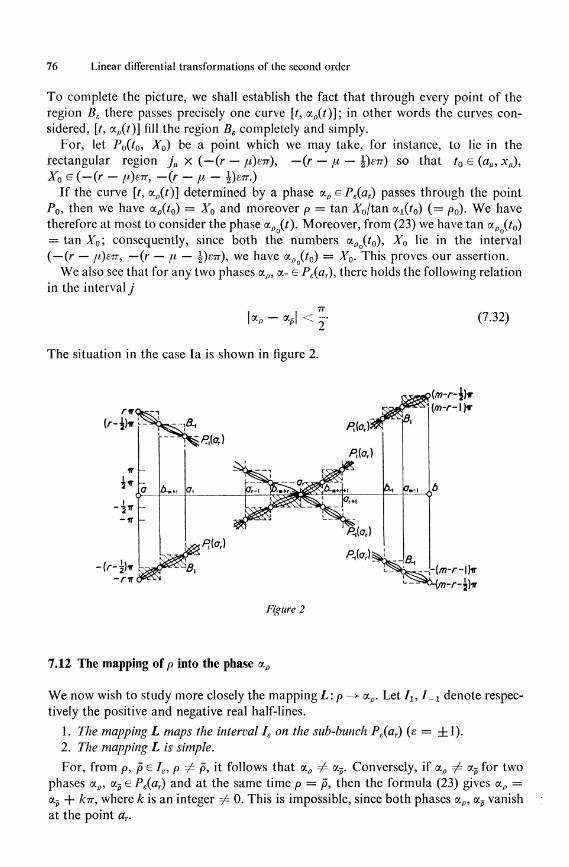
To complete the picture, we shall establish the fact that through every point of the region Be there passes precisely one curve [t, a^ t ) ] ; in other words the curves considered, [t, o:p(t)] fill the region Be completely and simply.

For, let P0(t0, X0) be a point which we may take, for instance, to lie in the rectangular region j u x (—(r — /U)S7T), — (r — fi — 1)STT) so that t0 e (au, xlt), X0 e (—(r — fi)en9 — (r — fi — \)err.)

If the curve [t, ap(t)] determined by a phase OLP ePe(ar) passes through the point P0, then we have ap(t0) = X0 and moreover p = tan X0/tan cc^to) ( = p0). We have therefore at most to consider the phase ocPo(t). Moreover, from (23) we have tan OLP (t0) = tan X0; consequently, since both the numbers ap (t0), X0 lie in the interval (—(r — fi)BTr, — (r — ft — \)STT), we have oLPo(t0) = X0. This proves our assertion.

We also see that for any two phases OLP, OL- E Pe(ar), there holds the following relation in the interval j

Ҝ - apl < 2 (7.32)

The situation in the case la is shown in figure 2.

-lr-łW

(m-r~{)v [m-r-\)w

Ľ ^ ^ - _ : - ( / 7 , - Г - І ) I Г

[m-r-{)if

Figure 2

M2 The mapping of p into the phase OLP

We now wish to study more closely the mappingL: p -> <xp. Let h.I^i denote respectively the positive and negative real half-lines.

1. The mapping L maps the interval Ie on the sub-bunch Pe(ar) (e = ±1). 2. The mapping L is simple.

For, from p, p e Ie, p ^ p, it follows that OLP ^ a-. Conversely, if OLP # a- for two phases onp9 OLP G Pe(ar) and at the same time p = p, then the formula (23) gives OLP = OL~P + kir, where k is an integer ^ 0. This is impossible, since both phases OLP, a-- vanish at the point ar.


3. For p, pe Iejp < p in every interval j u orj'fl (/i = 0, 1, . . .) there holds the relation ap < a? or ap > a~ respectively.

For, obviously tan ax > 0 or tan a± < 0 in every intervalj, orj^ respectively; then, taking account of (23), our assertion follows.

The sub-bunch Pe(ar) admits of the following ordering relation, denoted by ~<: for a, a e Pe(aT) we have a -< a if and only if the inequality a < a or a > a holds in every interval^ orj^? respectively.

The mapping L is order-preserving with respect to this ordering.

4. We define a metric in the set Ps(ar), by means of the formula

dfap. ap) = SUP K ( 0 ~ a/5(/)|.

In the interval Ie we adopt the usual Euclidean metric. We now show that:

The mapping L is homeomorphic.

Proof, (a) Let p, pele be arbitrary numbers. At every point tej other than

<*u + i> xu if1 = 0, 1 , . . .) we have the relation

tan (ap — aP)

whence, taking account of (32),

K — a?\ < t a n K — a? I =

From these relations it follows that

tan ap — tan a-

1 + tan aß tan aP

P - P

- + pp-u v

p — p\ V

u + pp u

V

\p - p\

Vppt \ + 2y/pp

A( \ - l IP - R 2 Vpp

(7.33)

so that the mapping L is continuous at every point p e Ie. (b) Let ap, a~pePe(ar) be arbitrary phases. Obviously, there exists a number t0 ej

such that tan OC IQ) = d ( = ±1). At this point t0 we have, from (23),

and further

ô(p — p) = tan aд — tan a- = (1 + pp) tan (a„ — aß)

= tan |ap — a-зl < tan d(ap, aҙ). i + pp

From these relationships it follows that

\P-P\

1+PP < tan d(aй, a?); (7.34)


hence the mapping L"1 is continuous at every point o^ePe(ar). This completes the proof.

7.13 Relations between zeros and boundary values of normal phases

In the course of our study of singular normal phases we encountered certain relations between the zeros and boundary values of these phases. For instance, Figure 2 shows that in the case we have considered every increasing or decreasing normal phase with the zero ar possesses the boundary values — m, (m — r — |)TT or m, —(m —• r — |)TT. We now study in greater generality the relations between zeros and boundary values of normal phases.

Consider a differential equation (q) of finite type (m), m > 1, or a left or right oscillatory differential equation, The left and right 1-fundamental sequences of (q), if they exist, we denote by

(a < ) rx = ax < a2 < * •# and (h > ) sx = b-x > b„2 > * •' •

Let a be a normal phase of (q), t0 ej its zero, and c, d its left and right boundary values. For simplicity, we put e = sgn oc' and use the symbol ^ to mean < when e = + 1 , > when s = —-1; similarly ^ means > when e = + 1 , and < when e = — 1.

(a) First we assume that the differential equation (q) is of finite type or is right oscillatory. In these cases the boundary value c is finite.

If the differential equation (q) is of type (1), and so without conjugate numbers of the first kind, then obviously we have the relations

s* $ c $ 0.

COП-

We now assume that the differential equation (q) admits of 1-conjugate numbers Let r > 0 be the integer defined by the stipulation t0 e (ar, ar + 1]; a0 = a. We c

sider the left null phase a0 included in the system [a]:

a 0 (0 = a(f) — c.

We clearly have the relations

a0(ar) £ oto(lo) £ a0(ar + i),

in which equality holds if and only if t0 = ar + 1. It follows, when we take account of the monotonicity of a0 and formula (10), that the two following relations hold simultaneously

ar < t0 < ar + 1; —(r + \)TTS § c § —me.

(b) Secondly, we assume that the differential equation (q) is of finite type or left oscillatory. In these cases the boundary value d is finite.

As above, we find that if the differential equation (q) is of type (1) then we have

0 § d $ rre.


If the differential equation (q) admits of 1-conjugate numbers, then there hold simultaneously the formulae

Z?_s_i < t0 § b^.s; sire ^ d § (s + 1)TT£ (S > 0; b0 = b),

in which both equality signs must be taken at the same time! These results may be summed up:

Theorem. Between the zero t0 ej and the boundary values c, d of a normal phase a of the differential equation (q), there hold the relations set out below, corresponding to the following table of type and kind of the differential equation (q):

I. finite type (m), m > l ; (a) general (b) special; II. infinite type; (a) right oscillatory (b) left oscillatory (c) oscillatory;

I. The boundary values c, d are finite.

(a) There hold the relations (m — \)TTS ^ d — c § mne, and when

m = 1: t0 ej, — TTS ^ C ^ 0 § d § TTB;

m > 2: ar < t0 < b-m+r + 1; —(r + \)TTS § c $ — we; (m — r __ i)^^ ^ / ^ (m — r)--£

or

b-m + r + l < tO^^r + i ; ~ ( r + -)™5 | C ^ — r7T_;

(m __. r —. 2)7rE $ d ^ (m — r — 1)TT£.

(b) JVe Aave d — e = mTre at/d

ar < to ^ #r + iJ ~~(r + I)77"6 :$ c >• —rTre; d = c + m7r£.

II. ^4t /easl orle of the boundary values c, d is infinite.

(a) ar < to < ar + 1; — (r + 1)TT£ ^ c ^ —rTre; d = Eoo.

(b) b_r^i < to < b^r; me ^ d § (r + \)TTE; C = — £oo,

(c) t0ej; c = -goo , r / = £oo.

7.14 Boundary characteristics of normal phases

Let a be a normal phase of the differential equation (q), t0 e j its zero and c, d its left and right boundary values. The ordered triad (t0; c, d) we shall call the boundary characteristic of the normal phase a; we shall use for it the notation ^(a), or more briefly %. The elements c, d are the essential terms of %((£). It is convenient also to speak of the values c, d when they denote the symbols + oo or — oo.

From the above results, we see that there exist certain relationships between the terms of ^(a), according to the type of the differential equation (q). In particular, for all types of the differential equation (q), we have a(f0) = 0, sgn a' = — sgn c = sgnd.


We now wish to study how far the normal phase a is determined by these relations. By a characteristic triple of the differential equation (q) we mean an ordered triad

(i0; c9 d) whose terms satisfy the appropriate conditions I(a)-II(c) of § 7.13, according to the type and kind of the differential equation (q). Naturally, t0 e j and c, J may denote the symbols ± oo; also e = sgn ( d— c).

Obviously, the boundary characteristic %(ci) represents a characteristic triple of (q). The question which we now examine is: given any characteristic triple % of the differential equation (q), do there correspond normal phases with the boundary characteristic #? If so, how may these normal phases be determined?

7.15 Determination of normal phases with given characteristic triple

Let x = (hi c? d) be a characteristic triple of the differential equation (q). We assume that there does indeed exist a normal phase a of (q) with the boundary characteristic X. Let (i/0, v0) be the basis of the differential equation (q) determined by the initial values

w0(t0) == 0, u0(t0) = - s g n c; v0(t0) = 1, v0(t0) = 0

and a0 be the phase of (u0, v0) which vanishes at the point t0: a0(t0) = 0. Obviously, a0 is a normal phase of (q) and we have sgn a0 = —sgn c. We denote by ^(a0) = (to» co> d0) the boundary characteristic of a0. We have —sgn c0 = sgn a0 = —sgn c and consequently sgn c0 = sgn c, sgn d0 = sgn d.

The functions a, a0 are, however, phases of the same differential equation (q); it follows that if one of the numbers C, c0 or d, d0 is finite, so is the other. Further, the following formula holds in the interval j , except at the singular points of tan a(t), tana0( t) ;

c±1 tan a0(t) + c12

tan a(t) = ~~——., c21 tan a0(t) + c22

with appropriate constants cll9 c129 c2l9 c22. (See § 5.17, corollary 4). Now c12 = 0, since both phases a, a0 vanish at the point t0. Obviously c22 ^ 0,

and we can assume that c22 = 1, because the numerator and denominator may be divided by c22- So we have

,,v Cu tan a0( t) tan a(t) c21 tan a0(t) + 1

This formula can be put into the following form, valid for all t ej

sin a0(t) • [Cn cos a(t) — c21 sin a(t)] = cos a0(t) sin a(t).

If the numbers c9 c0 or d, d0 are finite then this relation gives, respectively,

sin C0 • [Cn cos c — c21 sin c] = cos C0 • sin cA

sin d0 • [ctl cos d — c21 sin d] == cos d0 • sin d./

We observe that the constants cll9 c2l9 satisfy one or both of the linear equations (35) according to the type and kind of the differential equation (q) and are more or


less determined by the boundary values c, cQ or d9 dQ. We now wish to study this situation in the various cases.

We use the notation of §7.13. In particular, we put e = sgn a0 = sgn a and denote the 1-fundamental sequences, if they exist, by (a <) r± = ax < a2 < • • % (b>)s1 = b-1>b-2> •••. .

I. Finite type (m)9 m > 1

c, d nite, (m — 1)TTS § d — C ^ m7rE.

(a) General case: (w — 1)7TE § d — c ^ niTTS. (136)

1. m = 1: sin c sin d =£ 0, l0 ej, sin r0 sin d0 .^ 0.

2. m > 2 :

a) sin c sin d ^ 0, _»_m + r + 1 -^ 10 ^ ar + 1, sin c"0 sin dQ ^ 0,

/?) sin c 7 0, sin d = 0; l0 = b~~m + r + i < ar + 1; sin C0 -^ 0, sin dQ = 0,

y) sin C = 0, sin d =£ 0; b_m+r + 1 < 10 = ar + 1 ; sin cQ = 0, sin d0 # 0.

In cases 1 and 2a) the equations (35) can be written as follows

clx cot c — c21 = cot Co,) 7 . (737)

Cu cot a — c21 = cot a0.j From (36) we have cot c — cot d -?- 0. It is clear that the constants cll9 c21 are uniquely determined.

In the respective cases 2(1) (2y)) the first (second) equation (35) can be replaced by the first (second) equation (37) while the second (first) equation (35) is satisfied identically. Clearly, of the two constants cll9 c2l9 one is undetermined.

(b) Special case: d — c = mire = d0 — c0.

1. m = 1: sin c sin d =£ 0, t0 ej, sin cQ sin dQ -^ 0.

2. #w > 2 :

a) sin c sin rf^O; ar < f0 < ar + 1, sin cQ sin d0 ^ 0.

ft) sin C = sin d = 0; 10 = ar + 1, sin c0 = sin d0 = 0.

In the cases 1 and 2a) the equations (35) are linearly dependent and can be replaced by one of the equations (37). Clearly, of the constants cll9 c2l9 one is undetermined. In the case 2/5) the equations (35) are satisfied identically: the constants cll9 c21 are arbitrary.

II. Infinite type

At least one of the boundary values c9 d is infinite,

(a) Right oscillatory differential equation:

-—(r + \)TTB ^ c § —rTrs; d = eoo.

1. sin c ^=- 0, ar < t0 < ar + 1; sin c0 ^ 0.

2, sin c = 0, t0 = ar + 1; sin cQ = 0.


Clearly, in case 1 one of the constants cll9 c2l is undetermined, in case 2 both are arbitrary.

(b) Left oscillatory differential equation:

sirs ^ d ^ (s + 1)TTE; C = —ECO.

L sin d ^ 0, b^s^t < t0 < b^s; sin d0 i=- 0.

2. sin d = 0, to = 6 - s - i ; $m d0 = 0.

Clearly, in case 1 one of the constants cll9 c21 is undetermined, in case 2 both are arbitrary.

(c) Oscillatory differential equation:

to ej; c = —-coo, d = £co.

In this case both the constants cll9 c21 are arbitrary.

These results may be collected together as follows:

Theorem. For every characteristic triple % = (t0; c9 d) of the differential equation (q) there exist corresponding normal phases of (q) with the boundary characteristic %. According to the type and kind of the differential equation (q) and according as to whether t0 is singular or not9 there is precisely one normal phase or there is precisely one system of normal phases (containing one or two parameters) of the differential equation (q) with the boundary characteristic %. More precisely:

There is precisely one normal phase of the differential equation (q) with boundary characteristic %9 if(q) is a general differential equation either of type (1), or of type (m)9

m > 2, t0 not being singular. There are precisely GO1 normal phases of the differential equation (q) with the boundary

characteristic %9 if(q) is a differential equation of type (m)9 m > 2, and t0 is singular, or if the differential equation (q) is special of type (1) or of type (m)9 m > 2, t0 not being singular; this is also true if the differential (q) is left or right oscillatory and t0 is not singular.

There are precisely oo2 normal phases of the differential equation (q) with boundary characteristic %9 if(q) is special of type (m)9 m > 2, and t0 is singular; this is also true if the differential equation (q) is left or right oscillatory and the number t0 is singular; finally this is also true if the differential equation (q) is osciUatory.

7.16 Determination of the type and kind of the differential equation (q) by means of the boundary values of a phase of (q)

We now show that, given the boundary values of a phase of the differential equation (q) the type and kind of (q) is uniquely determined.

Let (q) be a differential equation, a a phase of (q) and e, dthe left and right boundary values of a.


Theorem. Let the numbers c, d be finite z then the differential equation (q) is of finite type (m), m > 1, and is general with\ m = f|d — C\\TT] + 1 or special with m = |d — C\\TT according as \d — c\ cannot or can be divided by TT. If C is finite and d infinite, then the differential equation (q) is right oscillatory; ifc is infinite and dfinite then (q) is left oscillatory, If c, d are both infinite then (q) is oscillatory.

Proof We first assume the numbers C, d are finite. Then, from the theorem of § 7.13, the differential equation (q) is of finite type (m), m > 1.

We choose A so that C* = c + A, d* = d + A have different signs. Then c*, d* are the boundary values of the normal phase a* = a + A of (q); let t0 be the zero of a*.

If the differential equation (q) is general, then from the theorem of § 7.13 we have

(m — 1)TTS § d* — c* ^ mire (e = sgn (d* — c*));

from which it follows that |d — c\ is not divisible by TT and m has the value [\d-c\l<n]+\.

If the differential equation is special, then from the same theorem we have

d* — c* = mire;

in this case |d — c\ is divisible by TT and m has the value \d — c|/V. Secondly we assume that at least one of the numbers c, d is infinite. In this case

our assertion follows immediately from the theorem of § 7.13. In particular we have: a differential equation (q) of finite type (m), m > 2, is

general or special according as the oscillation 0(a) of each of its phases a satisfies the relations

(m — \)TT < 0(a) < m7r or 0(a) = mir.

From the definition of § 7.2, this statement is also true for m = 1.

7.17 Properties of second phases

In the study of local and boundary properties of second phases of the differential equation (q), we make use of similar ideas and methods to those employed with respect to the first phases. We shall therefore abbreviate the discussion and bring out only a few of the relevant concepts and results. We assume from now on that the carrier q of the differential equation (q) is always non-zero in the interval j , and satisfies further properties according to circumstances. In particular, we shall recall that in the case q e C2 the associated differential equation (qx) of (q) exists and the first phases of this differential equation (qx) represent the second phases of (q) (§ 5.11).

(a) Theorem on the unique determination of a second phase from the Cauchy initial conditions.

Let t0 ej; Z0, Z0 ^ 0, Z'0 be arbitrary numbers. We assume the existence ofq'(t0). There exists precisely one second phase ft of the differential equation (q) which satisfies

at the point t0 the Cauchy initial conditions:

/?(t0) = Z0, /3'(to)=Z0, nto)^K (738)

f [x] denotes here, of course, the greatest integer not exceeding x. (Trans.)


This phase p is included in the second phase system of the basis (w, v) of the differential equation (q):

u(t) = sin Z0 • u0(t) +

v(t) = cos Z0 • u0(t) +

qi.t0)

1

qUÕ)

Z'0 cos Z, i M t o ) z ; \ . •

° + 2te-žlJSmZ° z ° s i n Z o + 2l^)-ž;)cosZo .

»o(0,

v0(t),

(7.39)

1/2 which w0> Vo are integrals of(q) determined by the initial values

u0(t0) = 0, u'0(t0) = 1; v0(t0) = 1, v'0(t0) = 0,

(b) Let /? be a second phase of the differential equation (q).

Assuming, as above, that q(t) =£ 0, t ej\ p is an increasing or decreasing function in the interval j ( = (a, b)). The finite or infinite limiting values

c' = lim p(t) and d' = lim 0(t)

are called respectively the left and r/g/it boundary values of (3. The circumstances under which these boundary values are finite or infinite are

analogous to those for the first phases. In particular, we have the following fact: let the differential equation (q) possess 2-conjugate numbers; then the boundary value c' (d') of p is finite if and only if the left (right) 2-fundamental number r2(s2) of (q) is proper.

The number \c' — d'\ is known as the oscillation of the phase /? in the interval/ The notation used is 0(fi\j)9 more briefly O(jS).

(c) The left (right) boundary values of the second phases of a left (right) principal basis of the second kind of the differential equation (q) are integral multiples of the number TT.

The right (left) boundary values of the second phases of a 2-principal basis, whose first term is a left (right) 2-fundamental integral, are odd multiples of |7r.

(d) We define second normal phases of the differential equation (q) and their boundary characteristics in a similar manner to those of first phases. With regard to the structure of the set of singular second normal phases, and the determination of second normal phases by their boundary characteristics, there are analogous results to those for first phases (§§ 7.9-7.15).

7,18 Relations between the boundary values of a first and second phase of the same basis

Let (u, v) be a basis of the differential equation (q) and a, /J be first and second phases of (u, v). We choose the phases so that in the interval j the relations

0 < p(t) - a (0 < TT (7.40)

hold; that is to say, we are dealing with two neighbouring phases of the mixed phase system of (w, v) (§ 5.14).


We know that the functions y{t), y'{t) constructed with arbitrary constants kl9 k2

sin [a{t) + k2] У(t) = kл

У'(t) = ±ki V\q(t)

VW(T)\ ' ' (7.41)

sin [0(0 + k2] '

V\p'(t)\

represent the general integral of (q) and its derivative. We now assume that the function q is negative throughout the intervalj Then the

phases a, /? either both increase or both decrease, i.e. sgn a' sgn /?' = 1. Let c9 cf and d, df be the left and right boundary values of a, /?. We know that the

two numbers c, cf and also d, d' are simultaneously finite or infinite. We consider the first case and assume from here onwards that the boundary values

c9 c or d, df are finite. It then follows from (40) that

0 ^ c' - c ^ IT, or 0 ^ d' - d ^ n.

We now show that: The relation c' = c {df = d) holds if and only if the left (right) 3-fundamental number

r3 {s3) o/(q) /8 improper. In this case, we have therefore the situation described in § 3.8. a = r3j r± = r2< r± (b = s3, s4 = s2 > sx).

The relation c' = c + TX {d' = d + rr) holds if and only if the left (right) 4-fundamental number r4 (s4) o/(q) l*8 improper. In this case, we have a = r4, r3 = rx < r2 (b = 84, S3 = 8! > S2).

Proof We restrict ourselves to proving the statements regarding the left boundary values c, cf.

First we note that each of the relations c = c, cf = c + -n is invariant with respect to a transformation a{t) = a{t) + A, @{t) = /3(r) + A of the phases a, (I, where A is arbitrary. One can, in particular, take I = —C, so without loss of generality we may assume c = 0. We shall also assume, for definiteness, that sgn a' = sgn j$f = 1.

(a) Let c' = c = 0. Let us select a number x ej; we thus have to show that there exists a number which is left 3-conjugate with x.

From the fact that c = 0 and sgn a' = 1 we have a{x) > 0. In the formulae (41) let us choose the constants k1? k2 as kx = 1, k2 = —a(x). Then we have an integral y of (q) which vanishes at the point x, and its derivative y'.

From (40), we have the inequality

P(x) - a(x) > 0. (7.42)

Since c' = 0 and sgn ft' = 1, the inequality ^(t) < ia(x) holds for every t ej in a right neighbourhood of a, and consequently

P(t) - a(x) < 0. (7.43)

From (42) and (43) we conclude that the left side of (43), regarded as a function of t, takes the value 0 at some point t0 e {a, x). The number t0 is obviously a zero of y' and consequently is a left 3-eonjugate number of x.

(b) Let a = r3. Then every number x ej possesses a left 3-conjugate number. We have to show that c' = 0.


We assume that c' > 0 and choose a number xej satisfying the inequality a(x) < \c'\ this is possible since c = 0 and sgn a' = 1. Next, in the formulae (41), we choose the constants kl9 k2 as kx = 1, k2 = — a(x). Then we have an integral y of (q) which vanishes at the point x, and its derivative y',

Now from the definition of c' and the fact that sgn (3' = 1 it follows that at every point t e (a9 x)

0 < - cf = c' — - c' < fi(t) - a(x) < P(x) - a(x) < TT,

and therefore 0 < p(t) — a(x) < TT. Obviously, the derivativey of y has no zero to the left of x; consequently x has no

left 3»conjugate number, which is a contradiction. (c) Let c' = TT. Let us choose a number x ej; we then have to show that x has a

left 4-conjugate number. Since c' = TT and sgn /?' = 1 we have /3(x) > 7r. In the formulae (41) we choose the constants kl9 k2 as kx = 1, k2 = — f}(x). Then

we have an integral y of (q) whose derivative yr vanishes at the point x. From (40) we have the inequality

a(x) - fi(x) > -TT. (7.44)

Since c = 0 and sgn a = 1 the inequality a(t) < \(P(x) — TT) holds for all t in a left neighbourhood of a, and consequently we also have

a(t) - P(x) < -TT. (7.45)

From (44) and (45) we conclude that: the left side of (45), regarded as a function of /, takes the value — TT at a point t0 e (a, x). This number t0 is obviously a zero of y and so represents a left 4-conjugate number of x.

(d) Let a = r4. Then to every number x ej there corresponds a left 4-conjugate number of x. We have to show that c* = TT.

We assume that c' < TT and choose a number x e j satisfying the inequality c' < P(x) < TT; since c' < TT and sgn /?' = 1, such a choice is possible.

Next, in the formulae (41) we choose the constants kl9 k2 as kx = 1, k2 = —/3(x). Then we have an integral j of (q) whose derivative y' vanishes at the point x.

Now, since c = 0 and sgn a' = 1, at every point t e (a9 x) we have

—TT < a(t) — TT < a(0 — j8(x) < a(x) — j3(x) < 0,

hence —TT < a(t) — /5(x) < 0. The integral y has therefore no zero to the left of x. Consequently there is no left

4-conjugate number of x9 which is a contradiction.

LinearDifferentialTransformationsoftheSecondOrder · 7.1 Unique determination of a phase from the...

Documents

Transcript of LinearDifferentialTransformationsoftheSecondOrder · 7.1 Unique determination of a phase from the...