Linear transformations and determinants Matrix multiplication as a
8
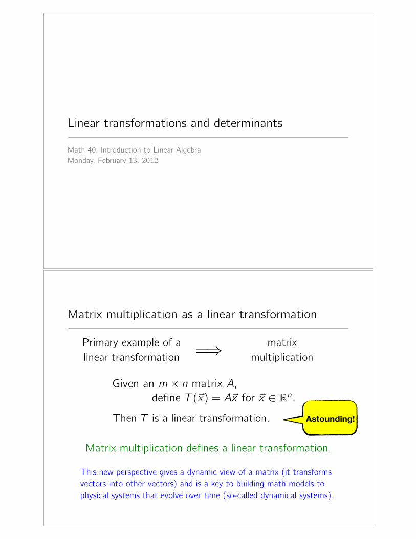
Linear transformations and determinants Math 40, Introduction to Linear Algebra Monday, February 13, 2012 Matrix multiplication as a linear transformation Primary example of a linear transformation = ⇒ matrix multiplication Then T is a linear transformation. Matrix multiplication defines a linear transformation. This new perspective gives a dynamic view of a matrix (it transforms vectors into other vectors) and is a key to building math models to physical systems that evolve over time (so-called dynamical systems). Astounding! Given an m × n matrix A, define T ( x )= A x for x ∈ R n .
Transcript of Linear transformations and determinants Matrix multiplication as a
Linear transformations and determinantsMath 40, Introduction to Linear AlgebraMonday, February 13, 2012
Matrix multiplication as a linear transformation
Primary example of a linear transformation =⇒
matrix multiplication
Then T is a linear transformation.
Matrix multiplication defines a linear transformation.
This new perspective gives a dynamic view of a matrix (it transforms vectors into other vectors) and is a key to building math models to physical systems that evolve over time (so-called dynamical systems).
Astounding!
Given an m × n matrix A,define T (�x) = A�x for �x ∈ Rn.
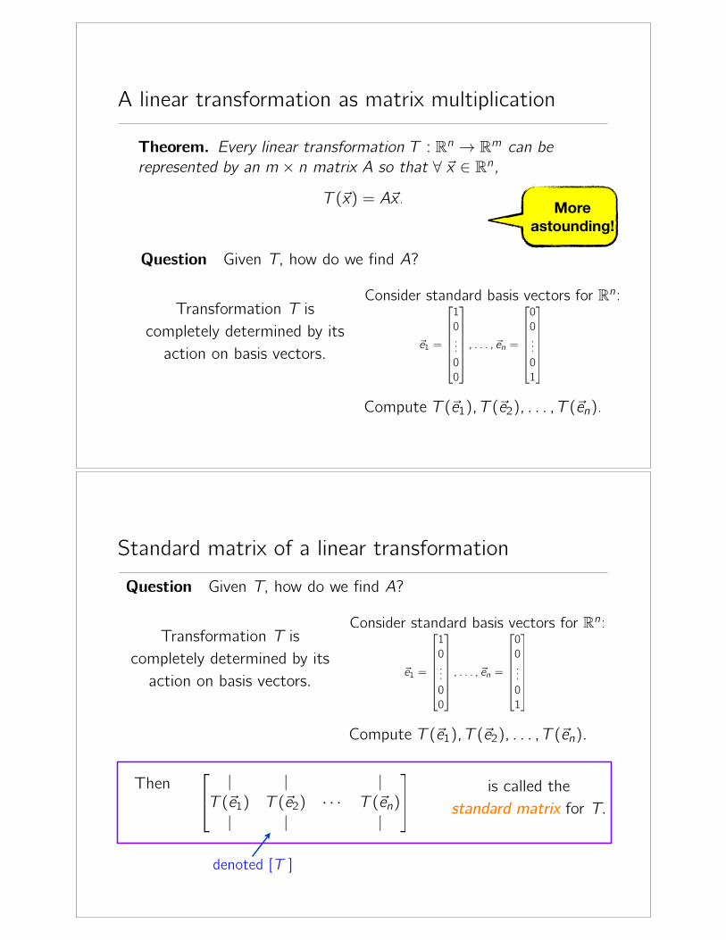
A linear transformation as matrix multiplication
More astounding!
Question Given T, how do we find A?
Transformation T is completely determined by its
action on basis vectors.
Consider standard basis vectors for Rn:
�e1 =
10...00
, . . . , �en =
00...01
Compute T (�e1), T (�e2), . . . , T (�en).
T (�x) = A�x.
Theorem. Every linear transformation T : Rn → Rm can berepresented by an m × n matrix A so that ∀ �x ∈ Rn,
Standard matrix of a linear transformation
Then is called the standard matrix for T.
Question Given T, how do we find A?
Transformation T is completely determined by its
action on basis vectors.
Consider standard basis vectors for Rn:
�e1 =
10...00
, . . . , �en =
00...01
Compute T (�e1), T (�e2), . . . , T (�en).
denoted [T ]
| | |
T (�e1) T (�e2) · · · T (�en)| | |
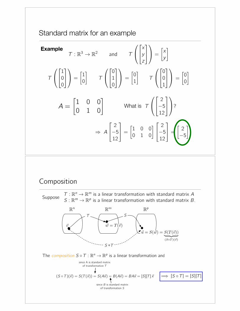
Standard matrix for an example
ExampleT : R3 → R2 and T
xyz
=�xy
�
T
100
T
010
T
001
=�00
�=
�01
�=
�10
�
A =
�1 0 00 1 0
�T
2−512
?What is
⇒ A
2−512
=�1 0 00 1 0
�
2−512
=�2−5
�
Composition
�v
Rn Rm Rp
T
�w = T (�v)
S
�u = S(�w) = S(T (�v))� �� �(S◦T )(�v)
S ⸰T
SupposeT : Rn → Rm is a linear transformation with standard matrix AS : Rm → Rp is a linear transformation with standard matrix B.
since A is standard matrixof transformation T
since B is standard matrixof transformation S
(S ◦ T )(�x) = S(T (�x)) = S(A�x) = B(A�x) = BA�x = [S][T ]�x
The composition S ◦ T : Rn → Rp is a linear transformation and
=⇒ [S ◦ T ] = [S][T ]
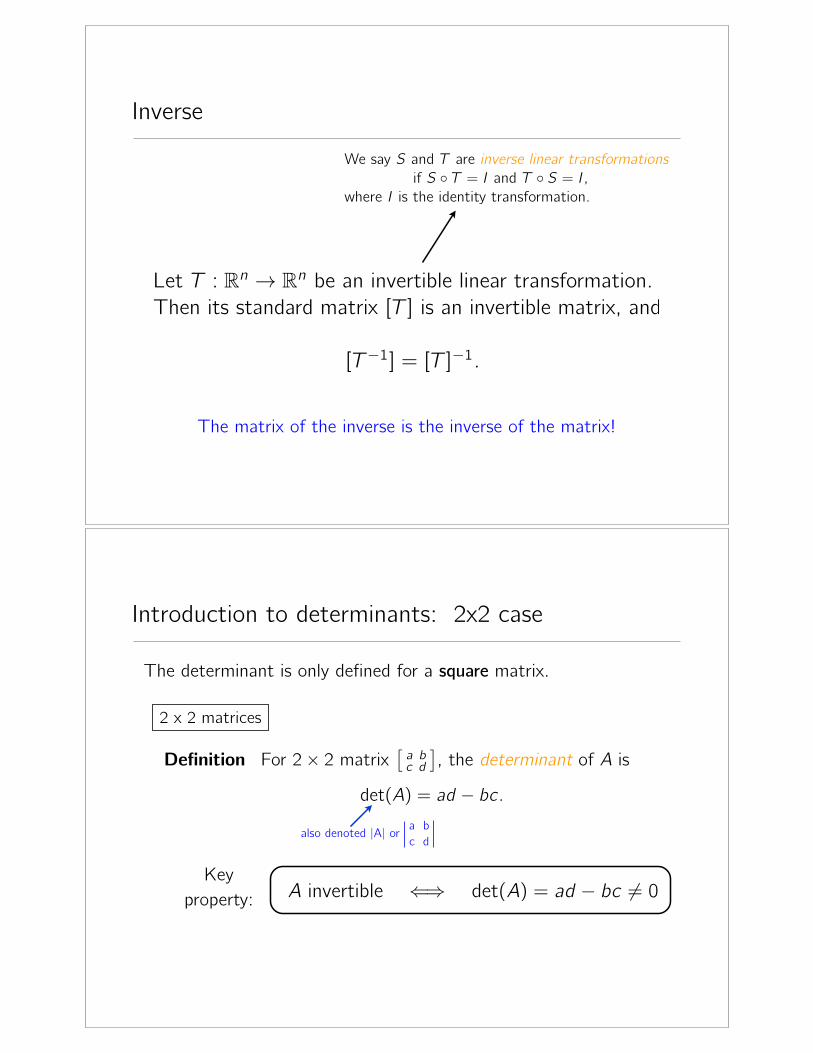
InverseWe say S and T are inverse linear transformations
if S ◦ T = I and T ◦ S = I,where I is the identity transformation.
The matrix of the inverse is the inverse of the matrix!
Let T : Rn → Rn be an invertible linear transformation.Then its standard matrix [T ] is an invertible matrix, and
[T−1] = [T ]−1.
Introduction to determinants: 2x2 case
The determinant is only defined for a square matrix.
2 x 2 matrices
det(A) = ad − bc.
also denoted |A| or a b c d
Key property: A invertible ⇐⇒ det(A) = ad − bc �= 0
Definition For 2× 2 matrix�a bc d
�, the determinant of A is
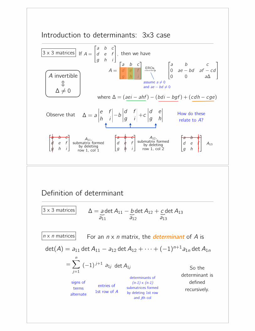
Introduction to determinants: 3x3 case
3 x 3 matrices A =
a b cd e fg h i
,If then we have
A =
a b cd e fg h i
EROs−−−→ A =
a b c0 ae − bd af − cd0 0 a∆
assume a �= 0and ae − bd �= 0
where ∆ = (aei − ahf )− (bdi − bgf ) + (cdh − cge)
A invertible�∆ �= 0
Observe that ∆ = a
����e fh i
���� How do these relate to A?
a b cd e fg h i
a b cd e fg h i
A11,submatrix formedby deletingrow 1, col 1
A12,submatrix formedby deletingrow 1, col 2
a b cd e fg h i
A13
−b����d fg i
����+c����d eg h
����
Definition of determinant
3 x 3 matrices{a11
{a12
{a13
n x n matrices For an n x n matrix, the determinant of A is det(A) = a11 detA11 − a12 detA12 + · · ·+ (−1)n+1a1n detA1n
∆ = a detA11 − b detA12 + c detA13
=n�
j=1
(−1) j+1 a1j detA1j
signs of terms
alternateentries of
1st row of A
determinants of (n-1) x (n-1)
submatrices formed by deleting 1st row
and jth col
So the determinant is
defined recursively.
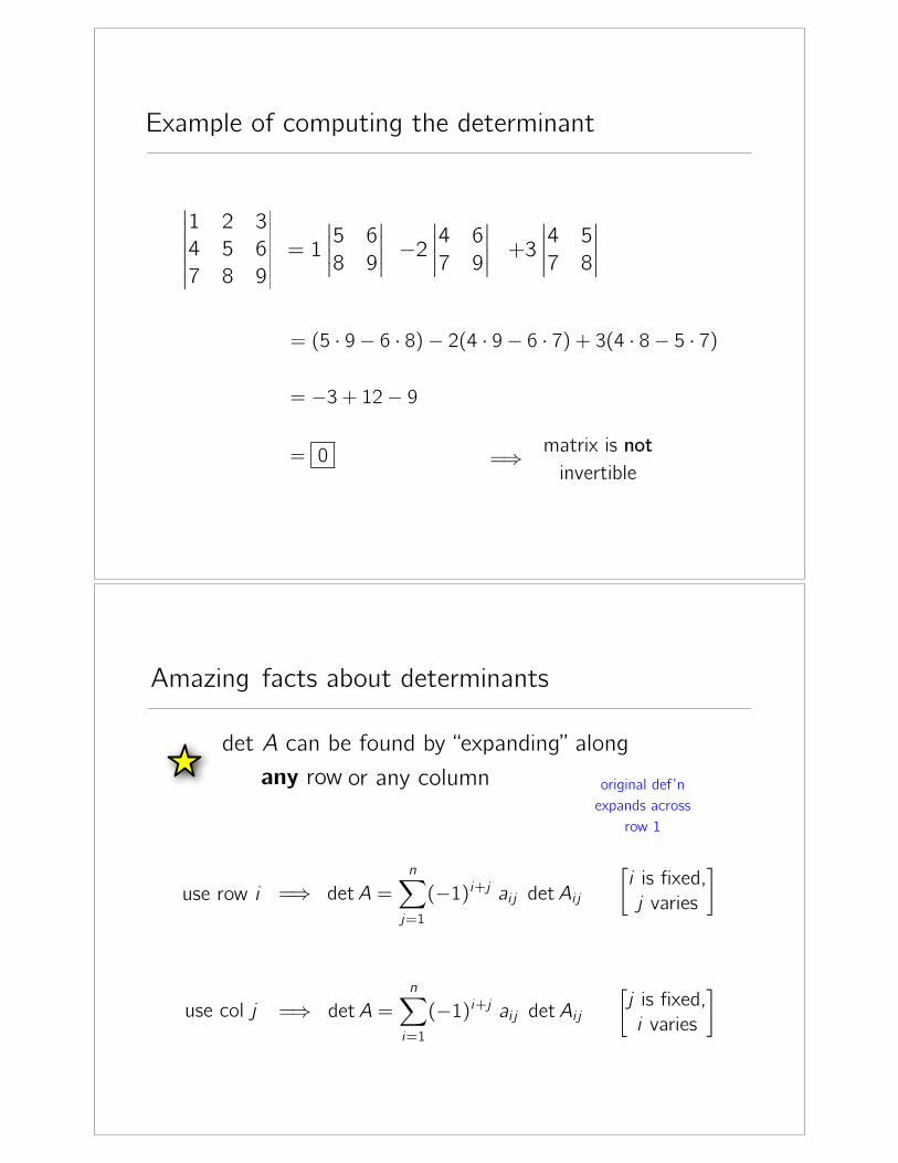
Example of computing the determinant
������
1 2 34 5 67 8 9
������= 1
����5 68 9
���� −2����4 67 9
���� +3����4 57 8
����
= (5 · 9− 6 · 8)− 2(4 · 9− 6 · 7) + 3(4 · 8− 5 · 7)
= −3 + 12− 9
= 0 =⇒ matrix is not invertible
facts about determinantsAmazing
det A can be found by “expanding” along any row or any column original def’n
expands across row 1
detA =n�
j=1
(−1)i+j ai j detAi j
detA =n�
i=1
(−1)i+j ai j detAi j
�i is fixed,j varies
�
�j is fixed,i varies
�
use row i =⇒
use col j =⇒
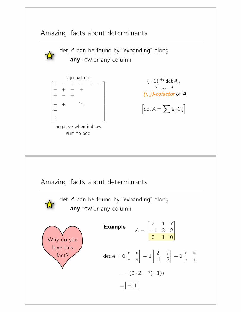
+ − + − + · · ·− + − ++ − +
− +.. .
+...
sign pattern
negative when indices sum to odd
(−1)i+j detAi j
�detA =
�ai jCi j
�
{(i, j)-cofactor of A
facts about determinantsAmazing
det A can be found by “expanding” along any row or any column
Why do you love this
fact?
Example A =
2 1 7−1 3 20 1 0
detA = 0
����∗ ∗∗ ∗
���� − 1����2 7−1 2
���� + 0����∗ ∗∗ ∗
����
= −(2 · 2− 7(−1))
= −11
facts about determinantsAmazing
det A can be found by “expanding” along any row or any column
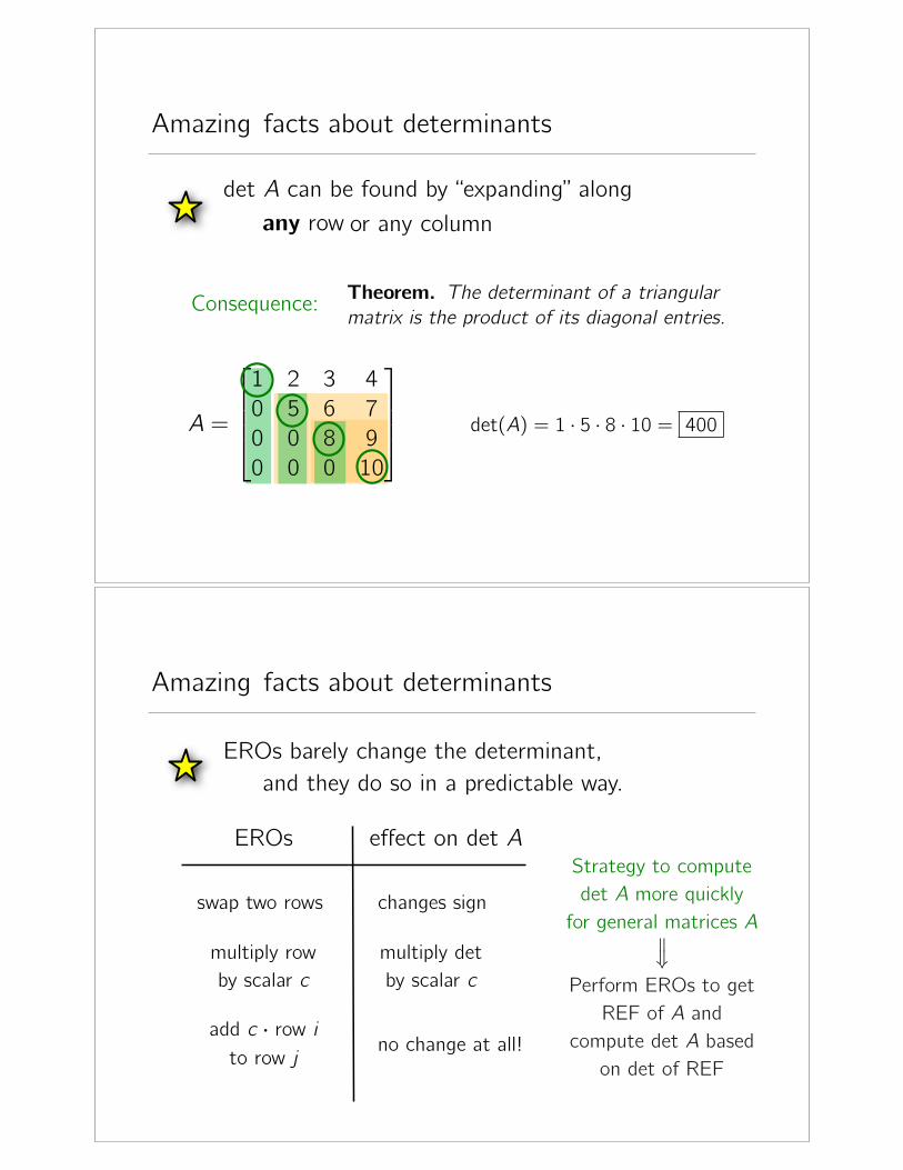
Consequence: Theorem. The determinant of a triangularmatrix is the product of its diagonal entries.
A =
1 2 3 40 5 6 70 0 8 90 0 0 10
det(A) = 1 · 5 · 8 · 10 = 400
facts about determinantsAmazing
det A can be found by “expanding” along any row or any column
EROs barely change the determinant, and they do so in a predictable way.
swap two rows changes sign
multiply row by scalar c
add c row i to row j
multiply det by scalar c
no change at all!
EROs effect on det AStrategy to compute det A more quickly
for general matrices A
Perform EROs to get REF of A and
compute det A based on det of REF
=⇒
facts about determinantsAmazing