
Linear Systems Control and Vibrations for Mechanical Engineers
90
Linear Systems Control and Vibrations for Mechanical Engineers Dr. Robert L. Williams II Mechanical Engineering, Ohio University NotesBook Supplement for ME 3012 Linear System Analysis, Control, and Vibrations © 2015 Dr. Bob Productions [email protected] people.ohio.edu/williar4 These notes supplement the ME 3012 NotesBook by Dr. Bob This document presents supplemental notes to accompany the ME 3012 NotesBook. The outline given in the Table of Contents on the next page dovetails with and augments the ME 3012 NotesBook outline and hence is incomplete here.
Transcript of Linear Systems Control and Vibrations for Mechanical Engineers

Linear Systems Control and Vibrations for Mechanical Engineers
Dr. Robert L. Williams II
Mechanical Engineering, Ohio University
NotesBook Supplement for ME 3012 Linear System Analysis, Control, and Vibrations
© 2015 Dr. Bob Productions
[email protected] people.ohio.edu/williar4
These notes supplement the ME 3012 NotesBook by Dr. Bob This document presents supplemental notes to accompany the ME 3012 NotesBook. The outline given in the Table of Contents on the next page dovetails with and augments the ME 3012 NotesBook outline and hence is incomplete here.
2
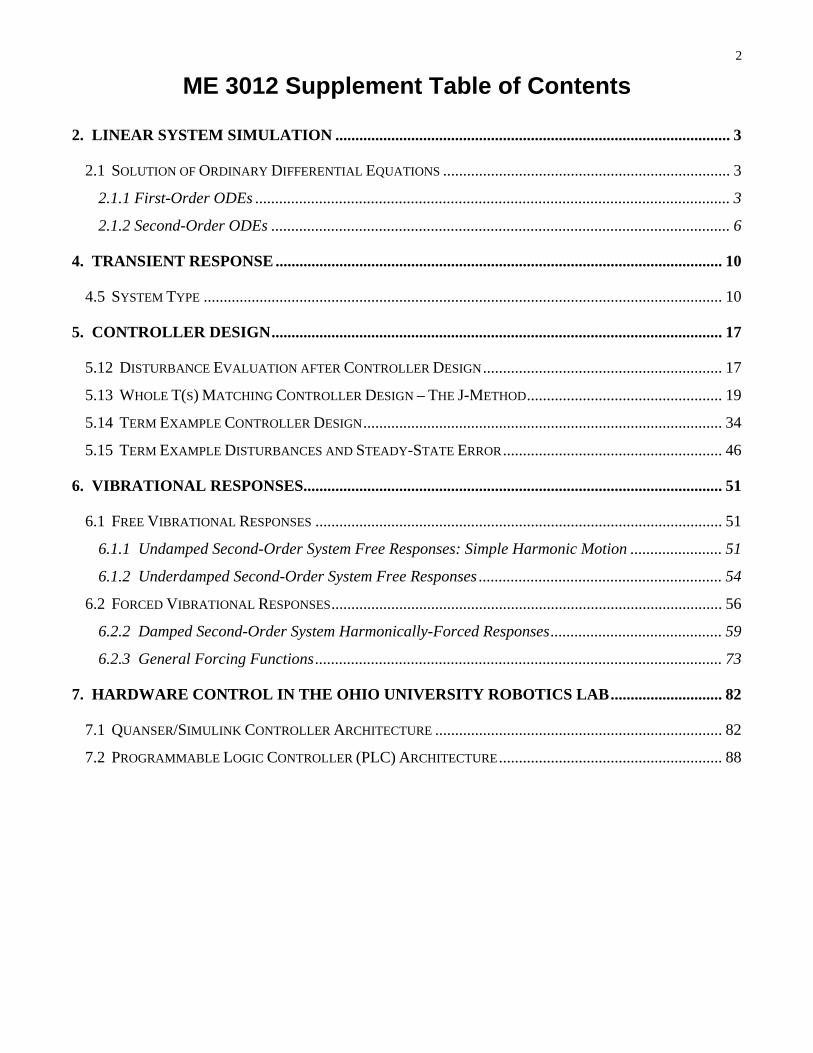
ME 3012 Supplement Table of Contents
2. LINEAR SYSTEM SIMULATION ................................................................................................... 3
2.1 SOLUTION OF ORDINARY DIFFERENTIAL EQUATIONS ........................................................................ 3
2.1.1 First-Order ODEs ....................................................................................................................... 3
2.1.2 Second-Order ODEs ................................................................................................................... 6
4. TRANSIENT RESPONSE ................................................................................................................ 10
4.5 SYSTEM TYPE .................................................................................................................................. 10
5. CONTROLLER DESIGN ................................................................................................................. 17
5.12 DISTURBANCE EVALUATION AFTER CONTROLLER DESIGN ............................................................ 17
5.13 WHOLE T(S) MATCHING CONTROLLER DESIGN – THE J-METHOD ................................................. 19
5.14 TERM EXAMPLE CONTROLLER DESIGN .......................................................................................... 34
5.15 TERM EXAMPLE DISTURBANCES AND STEADY-STATE ERROR ....................................................... 46
6. VIBRATIONAL RESPONSES......................................................................................................... 51
6.1 FREE VIBRATIONAL RESPONSES ...................................................................................................... 51
6.1.1 Undamped Second-Order System Free Responses: Simple Harmonic Motion ....................... 51
6.1.2 Underdamped Second-Order System Free Responses ............................................................. 54
6.2 FORCED VIBRATIONAL RESPONSES .................................................................................................. 56
6.2.2 Damped Second-Order System Harmonically-Forced Responses ........................................... 59
6.2.3 General Forcing Functions ...................................................................................................... 73
7. HARDWARE CONTROL IN THE OHIO UNIVERSITY ROBOTICS LAB ............................ 82
7.1 QUANSER/SIMULINK CONTROLLER ARCHITECTURE ........................................................................ 82
7.2 PROGRAMMABLE LOGIC CONTROLLER (PLC) ARCHITECTURE ........................................................ 88

3
2. Linear System Simulation 2.1 Solution of Ordinary Differential Equations 2.1.1 First-Order ODEs First-Order System Example 2 Same ck system and initial condition, but ( ) 5sin2f t t
Solve ( ) 50 ( ) 5sin2x t x t t subject to x(0) = 0
Solution
505( ) 25sin 2 cos 2
1252tx t e t t
Equivalent alternate solution form
505( ) 25.02sin 2 0.04
1252tx t e t using sin( ) sin cos cos sina b a b a b
The response x(t) starts at zero as specified by the initial condition. The transient solution goes to zero by about t = 0.10 sec. Steady-state solution is ( ) 25.02 sin 2 0.04ssx t t m.
= 2 rad/s = 2f f = 1/ = 1/T T = sec
0 1 2 3 4 5 6 7 8-0.1
-0.08
-0.06
-0.04
-0.02
0
0.02
0.04
0.06
0.08
0.1
t (sec)
-5/1252 cos(2 t)+125/1252 sin(2 t)+5/1252 exp(-50 t)
x(t)
(m
)

4
Alternate form for particular solution (Example 2)
Sum-of-angles formulae cos( ) cos cos sin sin
sin( ) sin cos cos sin
a b a b a b
a b a b c a b
25sin 2 cos 2 sin(2 )
sin 2 cos cos 2 sin
t t C t
C t t
sin 2 25 cos
cos 2 1 sin
t C
t C
2 2 2 2 2cos sin 25 1C 626 25.02C
sin 1
cos 25
1 1
tan 0.0425
rad
25sin 2 cos 2 25.02 sin 2 0.04t t t
In general: 2 21 2C B B 1 2
1
tanB
B
when
1 2( ) sin 2 cos2
sin 2Px t B t B t
C t

5
A Final First-Order ODE example R, C series electrical circuit (voltage v(t) input, current i(t) output)
Model (from KVL and electrical circuit element table) 1
( ) ( ) ( )Ri t i t dt v tC
substitute charge q(t) ( ) ( )
( ) ( )
i t dt q t
i t q t
1( ) ( ) ( )Rq t q t v t
C
Given R = 50 and C = 0.2 mF, solve 50 ( ) 5000 ( ) 1q t q t subject to (0) 0q and a unit step voltage input v(t). Solution
1001( ) 1
5000tq t e 1001
( ) ( )50
ti t q t e
As expected from the circuit dynamics, the charge q(t) in the capacitor builds up to a constant given a constant voltage input.
Also as expected, the capacitor current i(t) goes to zero at steady-state. The steady state charge value is qSS = 1/5000. The time constant is = RC = 0.01, so at 3 time constants (t = 0.03 sec) both the q(t) and i(t)
values have approached 95% of their respective final values.
v(t)
R
+-
i(t) C
0 0.01 0.02 0.03 0.04 0.05 0.060
0.5
1
1.5
2x 10
-4
q(t
)
0 0.01 0.02 0.03 0.04 0.05 0.060
0.005
0.01
0.015
0.02
i(t)
t (sec)

6
2.1.2 Second-Order ODEs Second-Order System Example 1 m = 1 kg, c = 7 Ns/m, k = 12 N/m
Solve ( ) 7 ( ) 12 ( ) ( ) 3 ( )x t x t x t f t u t subject to (0) 0.10
(0) 0.05 /
x m
x m s
This system is overdamped
Real distinct roots, relatively slower response, no overshoot
This solution is left to the interested reader.

7
Second-Order System Example 2 m = 1 kg, c = 6 Ns/m, k = 9 N/m
Solve ( ) 6 ( ) 9 ( ) ( ) 3 ( )x t x t x t f t u t
Subject to (0) 0.10
(0) 0.05 /
x m
x m s
1. Homogeneous Solution ( ) 6 ( ) 9 ( ) 0H H Hx t x t x t
Assume ( ) st
Hx t Ae 2( 6 9) 0sts s Ae
Characteristic polynomial 2 26 9 ( 3) 0s s s
1,2 3, 3s Real, repeated roots
Homogeneous solution form 3 3
1 2( ) t tHx t A e A te
2. Particular Solution ( ) 6 ( ) 9 ( ) 3P P Px t x t x t
( )Px t B 0 6(0) 9 3B so ( ) 1/ 3Px t B
3. Total Solution
3 31 2
3 3 31 2 2
( ) ( ) ( ) 1/ 3
( ) 3 3
t tH P
t t t
x t x t x t Ae A te
x t Ae A e A te
Now apply initial conditions
1 2
1 2
(0) 0.10 (0) 0.33
(0) 0.05 3
x A A
x A A
1
2
0.233
0.65
A
A
3( ) (0.233 0.65 ) 0.33tx t t e
This system is critically-damped
Real, repeated roots – fastest response without overshoot Check solution
Plug answer x(t) plus its two derivatives into the original ODE. Also check the initial conditions. Plot – check transient and steady state solutions, plus total solution.

8
Second-Order System Example 2 – Forced m-c-k System
Model ( ) ( ) ( ) ( )mx t cx t kx t f t
( ) 6 ( ) 9 ( ) 3 ( )x t x t x t u t (0) 0.10
(0) 0.05 /
x m
x m s
2 26 9 ( 3) 0s s s
Solution 3 1( ) (0.233 0.65 )
3tx t t e
Plot of x(t) vs. t
The total solution x(t) starts at 0.1 m, ( )x t is non-zero, as specified by the initial conditions.
Transient approaches zero after t = 2.5 sec Critically damped; –3 root goes to zero slightly faster alone than with t Steady-state value is xSS = 1/3 m.
0 1 2 3 4
-0.2
-0.1
0
0.1
0.2
0.3
0.4
t (sec)
x(t)

9
Second-Order System Example 4: Forced m-k System
Model ( ) ( ) ( )mx t kx t f t (no damping)
( ) 9 ( ) 3 ( )x t x t u t (0) 0.10
(0) 0.05 /
x m
x m s
2 9 ( 3 )( 3 ) 0s s i s i
Solution ( ) (7 30)cos3 (1 60)sin3 1 3x t t t
Plot of x(t) vs. t
x(t) starts at 0.1 m, ( )x t is non-zero, as specified by the initial conditions.
Simple harmonic motion Undamped; zero viscous damping coefficient Transient solution oscillates forever about the particular solution 1/3 = 3 rad/s = 2f f = 3/2 = 1/T T = 2/3 = 2.09 sec
This system is undamped
Complex-conjugate roots with 0 real part, simple harmonic motion, no damping, theoretically never stops vibrating.
10
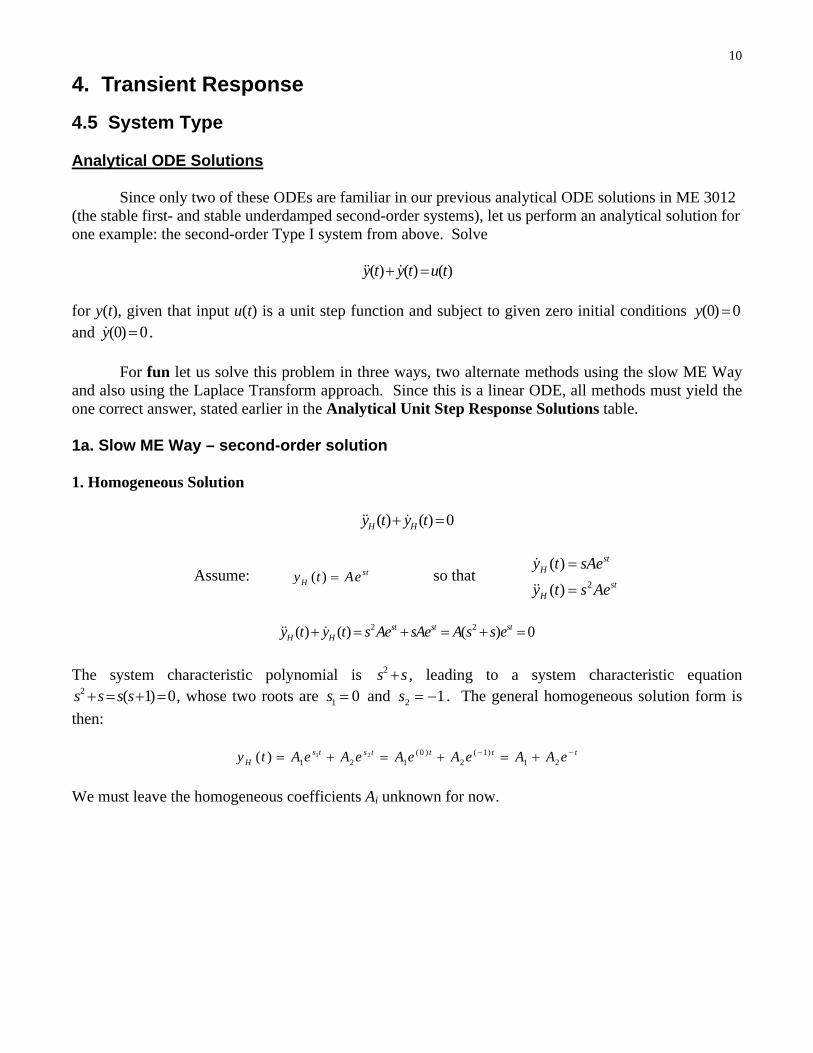
4. Transient Response
4.5 System Type Analytical ODE Solutions Since only two of these ODEs are familiar in our previous analytical ODE solutions in ME 3012 (the stable first- and stable underdamped second-order systems), let us perform an analytical solution for one example: the second-order Type I system from above. Solve
( ) ( ) ( )y t y t u t for y(t), given that input u(t) is a unit step function and subject to given zero initial conditions (0) 0y and (0) 0y . For fun let us solve this problem in three ways, two alternate methods using the slow ME Way and also using the Laplace Transform approach. Since this is a linear ODE, all methods must yield the one correct answer, stated earlier in the Analytical Unit Step Response Solutions table. 1a. Slow ME Way – second-order solution 1. Homogeneous Solution
( ) ( ) 0H Hy t y t
Assume: ( ) stHy t Ae so that
2
( )
( )
stH
stH
y t sAe
y t s Ae
2 2( ) ( ) ( ) 0st st st
H Hy t y t s Ae sAe A s s e
The system characteristic polynomial is 2s s , leading to a system characteristic equation
2 ( 1) 0s s s s , whose two roots are 1 0s and 2 1s . The general homogeneous solution form is
then:
1 2 ( 0 ) ( 1)1 2 1 2 1 2( ) s t s t t t t
Hy t A e A e A e A e A A e
We must leave the homogeneous coefficients Ai unknown for now.

11
2. Particular Solution
( ) ( ) ( ) 1P Py t y t u t
Our standard particular solution assumption of ( )Py t B will not work in this case so we immediately
try:
( )Py t B
where B is an unknown constant, which must be determined in this step. Clearly ( ) 0Py t and so:
( ) ( ) 0 1P Py t y t B
And so the particular solution for velocity is ( ) 1Py t B . However, we need the particular solution for
y(t), not its first derivative, and so we must integrate:
0 0( ) ( )
t t
P Py t y t dt dt t c
where c is a constant of integration, in this case left unknown until Step 3. 3. Total Solution
1 2( ) ( ) ( ) tH Py t y t y t A A e t c
An alert student may ask, how can we solve for three constants A1, A2, and c with only two initial conditions? The solution to this little dilemma is quite easy, recognizing that 1A c is simply a single
constant, call it 3 1A A c . Then the total solution is expressed by:
3 2( ) ty t A A e t
to which we apply the two given initial conditions (0) 0y and (0) 0y in order to solve for the unknown constants A1 and A3.
(0)3 2
2 3
(0) 0
0 (0)
0
y
A A e
A A
2( ) 1ty t A e (0)
2
2
2
(0) 0
0 1
1 0
1
y
A e
A
A
And since 2 3 0A A , we then have
3 2 1A A

12
and the total solution is: ( ) 1ty t e t
The transient part of this solution is te and the steady-state part of this solution is 1t . To demonstrate the transient and steady-state components of this solution better, it is instructive to plot this response, both its components and the total solution (which was shown previously, the center Type I case).
Detailed Plot for Center Type I System Example Unit Step Response Transient, Steady-State, and Total Responses

13
In order to check this solution, we can first check the resulting initial conditions. From the solution ( ) 1ty t e t we clearly see that 0(0) 0 1 1 0 1 0y e as required. Also, for the
first derivative of the solution ( ) 1ty t e , we have 0(0) 1 1 1 0y e as required.
A more complete solution check involves substituting the solution y(t) and its two time derivatives into the original ODE and prove than an equality results.
( ) 1
( ) 1
( )
t
t
t
y t e t
y t e
y t e
?( ) ( ) ( ) 1
1 1t t
y t y t u t
e e
Since an equality results, 1 = 1, this proves that the solution is the correct one.
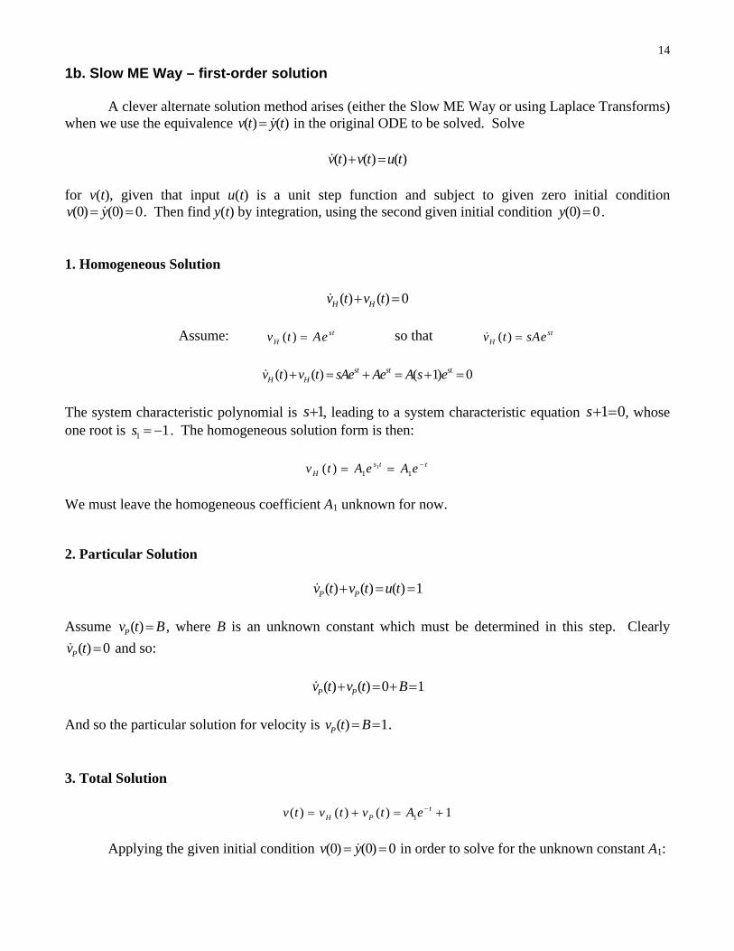
14
1b. Slow ME Way – first-order solution A clever alternate solution method arises (either the Slow ME Way or using Laplace Transforms) when we use the equivalence ( ) ( )v t y t in the original ODE to be solved. Solve
( ) ( ) ( )v t v t u t for v(t), given that input u(t) is a unit step function and subject to given zero initial condition
(0) (0) 0v y . Then find y(t) by integration, using the second given initial condition (0) 0y . 1. Homogeneous Solution
( ) ( ) 0H Hv t v t
Assume: ( ) st
Hv t Ae so that ( ) stHv t sAe
( ) ( ) ( 1) 0st st st
H Hv t v t sAe Ae A s e
The system characteristic polynomial is 1s , leading to a system characteristic equation 1 0s , whose one root is 1 1s . The homogeneous solution form is then:
1
1 1( ) s t tHv t A e A e
We must leave the homogeneous coefficient A1 unknown for now. 2. Particular Solution
( ) ( ) ( ) 1P Pv t v t u t
Assume ( )Pv t B , where B is an unknown constant which must be determined in this step. Clearly
( ) 0Pv t and so:
( ) ( ) 0 1P Pv t v t B
And so the particular solution for velocity is ( ) 1Pv t B .
3. Total Solution
1( ) ( ) ( ) 1tH Pv t v t v t A e
Applying the given initial condition (0) (0) 0v y in order to solve for the unknown constant A1:
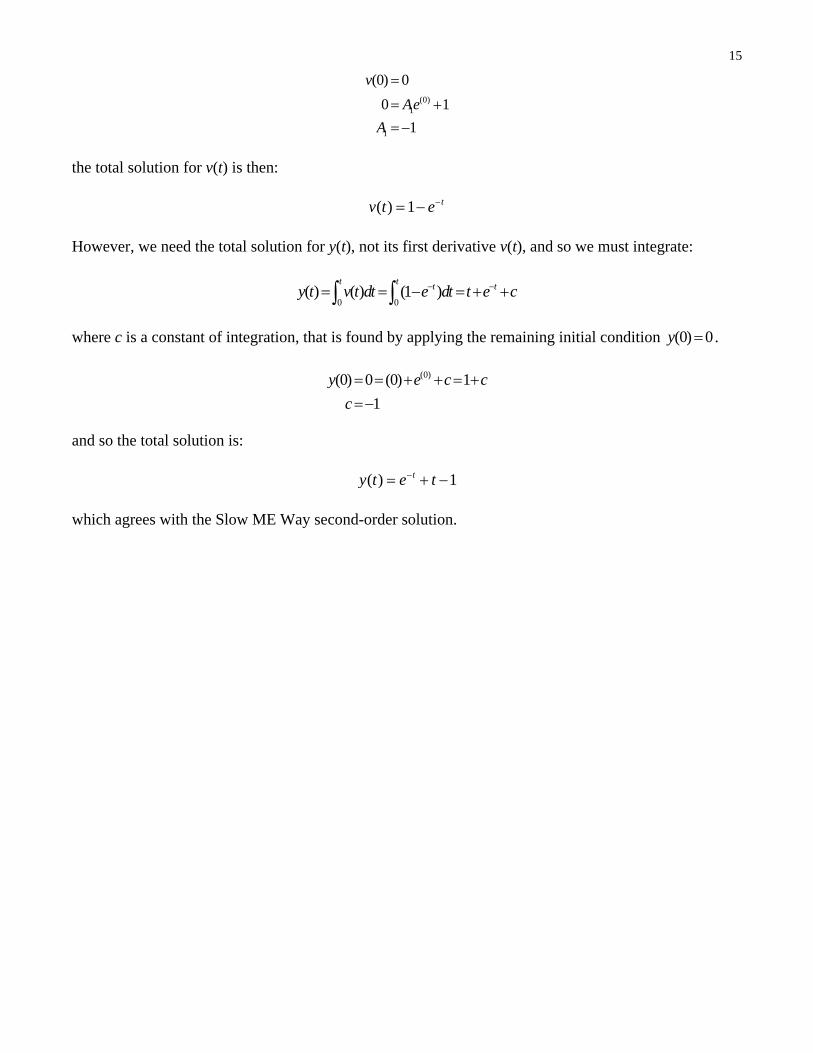
15
(0)1
1
(0) 0
0 1
1
v
Ae
A
the total solution for v(t) is then:
( ) 1 tv t e However, we need the total solution for y(t), not its first derivative v(t), and so we must integrate:
0 0( ) ( ) (1 )
t t t ty t v t dt e dt t e c
where c is a constant of integration, that is found by applying the remaining initial condition (0) 0y .
(0)(0) 0 (0) 1
1
y e c c
c
and so the total solution is:
( ) 1ty t e t which agrees with the Slow ME Way second-order solution.

16
2. Laplace Transforms solution Take the Laplace transform of both sides, with initial conditions.
2
( ) ( ) ( )
1( ) (0) (0) ( ) (0)
y t y t u t
s Y s s sY ss
Combine Y(s) terms on the left.
2 1( ) ( ) ( 1) ( )s s Y s s s Y s
s
Solve for the variable of interest, Y(s) – the Laplace transform of the answer, y(t).
2
1( )
( 1)Y s
s s
The partial fraction expansion for this Y(s) is given below, where the constants C1,2,3 are the residues.
31 22 2
1( )
( 1) 1
CC s CY s
s s s s
Express the partial fraction form over a common denominator.
2 23 1 2 3 1 3 1 2 21 2
2 2 2 2
( )( 1) ( ) ( )1( )
( 1) 1 ( 1) ( 1)
C C s C s C s C C s C C s CC s CY s
s s s s s s s s
Equate like powers of s in the numerator to get 3 equations to solve for the residues C1,2,3.
21 3
11 2
02
0
0
1
s C C
s C C
s C
1
2
3
1
1
1
C
C
C
Solution by inverse Laplace transform
1 1 1 1 131 22 2
1 1 1( ) ( )
1 1
CC s Cy t Y s
s s s s s
( ) 1 ty t t e
which agrees with the solutions we previously derived, but as expected is a more-direct one-stage process and faster to obtain.

17
5. Controller Design 5.12 Disturbance Evaluation after Controller Design General disturbance diagrams (open- and closed-loop)
Disturbance diagram with zero reference input This is called a regulator, where the desired output (reference input) is R(s) = 0.
Change this into a diagram that looks more similar to the standard closed-loop feedback diagram.
G(s)Y(s)U (s)U(s)
D(s)
D
-G(s)
H(s)
G (s)R(s) E(s) Y(s)U (s)
Y (s)
C
SENS Y(s)
U(s)
D(s)
D
G(s)
H(s)
G (s)E(s) Y(s)U (s)
Y (s)
C
SENS Y(s)
U(s)
D(s)
D
-1
G(s)
H(s)G (s)E(s)
Y(s)U (s)
Y (s)C
SENS Y(s)
U(s)
D(s) D
-1
+
+

18
The closed loop transfer function between the disturbance input D(s) and Y(s) output is:
( ) ( )( )
( ) 1 ( ) ( ) ( )DC
Y s G sT s
D s G s G s H s
This is for MATLAB implementation, to simulate the effects of the disturbance input separately. Then use linear superposition in MATLAB to find the total solution as the sum of the reference input response (with zero disturbance) plus the disturbance input (with zero reference input).

19
5.13 Whole T(s) Matching Controller Design – The J-Method Standard negative feedback closed-loop block diagram
Summary of controller design via parameter matching
Step 1. Analyze the as-given open-loop system behavior. Step 2. Specify and evaluate the desired behavior for the closed-loop system. This step
yields a numerical desired characteristic polynomial for the T(s) denominator, called DES(s). Step 3. Specify the form for the controller transfer function. Assume a standard form for
your controller GC(s). Step 4. State the controller design problem to be solved. Step 5. Solve for the unknown gains to achieve the desired behavior for the closed-loop
system. Derive closed-loop transfer function as a function of controller gains and parameters: ( ) ( )
( )1 ( ) ( ) ( )
C
C
G s G sT s
G s G s H s
Match the symbolic parameters in the denominator of T(s) with your numerical desired characteristic polynomial – term-by-term according to s powers (make sure both polynomials have the same leading coefficient for the highest s power).
Solve for the controller unknowns, determine the correction factor (if necessary), determine the pre-filter transfer function GP(s) (if necessary), and simulate the resulting performance.
Step 6. Evaluate the controller performance in simulation. Step 7. Include an output attenuation correction factor if necessary. Step 8. Include a pre-filter transfer function GP(s) if necessary. Repeat Step 6. Step 9. Re-design and re-evaluate the controller if necessary, if the performance specs are
not met. There are possible drawbacks with this method, the biggest being: the order of the closed-loop system must match the number of controller unknowns. If the number of unknowns is less, there is no solution (overconstrained) and if the number of unknowns is greater, there are infinite solutions (underconstrained). In either of the mismatch cases we can use trial-and-error controller design. This
can be frustrating and ineffective since there are n solutions, where n is the number of controller unknowns. See Section 5.10 in this ME 3012 NotesBook. Further drawbacks include the need for most standard controllers to add a correction factor for output attenuation and a pre-filter transfer function GP(s) to cancel the unwanted introduced zero(s). There is a potentially better method, here called the whole T(s) Matching Controller Design, or simply the J-Method. This is named after ME student Jason Denhart who, in Spring 2008, posed the question “Why can’t we just specify the entire numerical T(s) and solve for the exact GC(s) necessary to provide that T(s)?”
-G(s)
H(s)
G (s)R(s) E(s) Y(s)U(s)
Y (s)
C
SENS Y(s)

20
The J-Method Step 1. Analyze the as-given open-loop system behavior. Step 2. Specify and evaluate the desired behavior for the closed-loop system. This step
yields a numerical desired characteristic polynomial for the T(s) denominator (see Note 1 below), plus the desired T(s) numerator.
Step 3. State the controller design problem to be solved. The former Step 3 is skipped, i.e. the J-Method determines the controller form in the solution procedure so there is no need to assume a standard controller form for GC(s).
Given The plant and sensor transfer functions G(s) and H(s) in the context of our
standard closed-loop negative feedback diagram. The desired closed-loop behavior, expressed by a whole numerical T(s) (as
opposed to the desired closed-loop characteristic polynomial only as before). Find The form and the unknowns (gains) of the controller transfer function GC(s).
Step 4. Solve for the unknown controller form including the unknown gains. Use the standard equation
( ) ( )( )
1 ( ) ( ) ( )C
C
G s G sT s
G s G s H s
Substitute your whole numerical desired T(s), plus the known numerical plant and sensor transfer functions G(s) and H(s), and solve for the unknown controller transfer function GC(s), without the need to assume a certain controller form.
( )( )
( )(1 ( ) ( ))C
T sG s
G s H s T s
Step 5. Simulate the resulting closed-loop system performance. Step 6. Re-design and re-evaluate if necessary, if the performance specs are not met.
Notes 1. The order of the denominator of your desired T(s) must be equal or greater than the order of the denominator of G(s). If the G(s) denominator is of higher order than the T(s) denominator, your resulting GC(s) will have a higher order in the numerator than the denominator, which is impossible to implement in MATLAB or Simulink, unless it happens to boil down to a PID form. 2. You do not need a correction factor – this is loaded into your desired T(s). 3. You do not need a pre-filter transfer function GP(s) since we are matching the entire desired T(s). 4. The resulting controller GC(s) will not necessarily be of any recognizable classical controller form. 5. MATLAB was used to help with the algebra (either symbolically or numerically). This should work; however, problems were encountered with large integers and excessive controller numerator and denominator orders. 6. If you follow the requirement for T(s) denominator order and make no algebra mistakes, the performance you obtain will be theoretically identical to a good classical controller with appropriate pre-filter and correction factor. 7. There are three major drawbacks of the J-Method
The J-Method does not handle disturbances well, as most other controllers do (presented later). The J-Method requires perfect knowledge of the open-loop plant, which is impossible. Thus, it
is less robust to modeling uncertainties than other controllers. The J-Method cannot handle unstable open-loop plants (this is no problem for other controllers).

21
Controller Design Example 1 – The J-Method Step 1. Analyze the as-given open-loop system behavior.
This step is the same as in Controller Example 1, with 2
10( )
10G s
s s
.
Step 2. Specify and evaluate the desired behavior for the closed-loop system, to achieve 5% overshoot and 1.5 sec settling time. We have used these performance specifications before; the associated desired whole closed-loop transfer function is (assuming a final value of 1 is desired from a unit step input):
2
14.93( )
5.33 14.93T s
s s
Step 3. State the controller design problem to be solved.
Given 2
10( )
10G s
s s
, H(s) = 1, and
2
14.93( )
5.33 14.93T s
s s
Solve for GC(s) via whole T(s) matching. Step 4. Solve for the unknown controller form including the unknown gains.
The result is 21.493( 10)
( )( 5.33)C
s sG s
s s
What type of controller is this? How does the J-Method controller work?

22
Step 5. Simulate the resulting closed-loop system performance. Simulink Evaluation for the J-Method Controller Design Example 1
Simulink simulation results
Open-Loop Closed-Loop J-Method
There is no need for a correction factor or pre-filter.
Step1
Step
Scope
10
s +s+102
Plant2
10
s +s+102
Plant1
s +5.33s21.493*[1 1 10]
Gc

23
Examples To rigorously test the J-Method, the following three open-loop transfer functions G(s) and the following three desired whole closed-loop transfer functions T(s) were chosen, to be mixed-and-matched for a total of 9 examples.
G(s) T(s)
1. 1
1s a.
2
2s
2. 2
10
10s s b.
2
15
6 15s s
3. 2
10
( 1)( 10)s s s c.
3 2
450
36 195 450s s s
The whole desired T(s) in a. is based on a time constant of = 0.5 sec. The whole desired T(s) in b. started from our familiar specification of 5% overshoot and 1.5 sec
settling time (leading to a dominant second-order desired denominator of 2 5.33 14.93s s ). But I wanted nice integers for the multiple example combinations, so this one corresponds to 2.13% overshoot and 1.38 sec settling time ( = 0.78, n = 3.87 rad/s, and
1,2 3 2.45s i ).
The whole desired T(s) in c. started from b., augmenting the denominator with a third pole
3 30s , so approximately the same dominant second-order behavior will result (2.13%
overshoot and 1.38 sec settling time). All whole desired T(s) in a., b., and c. artificially obtain a steady state value of 1 give a unit step
input function, with selection of the numerator constant to match the denominator ‘spring’. Let’s do a few of these examples now. Assume unity negative feedback for all examples. Example 1a
Given open-loop plant 1
( )1
G ss
, ideal sensor transfer function H(s) = 1, and desired whole
2( )
2T s
s
, determine GC(s) via whole T(s) matching:
Answer 2( 1)
( )C
sG s
s
(what kind of controller is this?)

24
Simulink simulation results
Open-Loop Closed-Loop J-Method
The open-loop time constant of = 1 sec is halved to the closed-loop time constant of = 0.5 sec, which doubles the speed of the closed-loop system to reach 95% of the final value of 1.

25
Example 1b
Given open-loop plant 1
( )1
G ss
, ideal sensor transfer function H(s) = 1, and desired whole
2
15( )
6 15T s
s s
, determine GC(s) via whole T(s) matching:
Answer 15( 1)
( )( 6)C
sG s
s s
(what kind of controller is this?)

26
Simulink simulation results
Open-Loop Closed-Loop J-Method
The open-loop time constant was = 1 sec and the desired closed-loop performance specs of 2.13% overshoot and 1.38 sec settling time are met in simulation.

27
Example 2a
Given open-loop plant 2
10( )
10G s
s s
, ideal sensor transfer function H(s) = 1, and desired whole
2( )
2T s
s
, determine GC(s) via whole T(s) matching.
Answer 2 10
( )5C
s sG s
s
(what kind of controller is this?)
This is an exception to the rule that the T(s) denominator must of order equal or greater than the order of the G(s) denominator, since it is a PID controller.
28
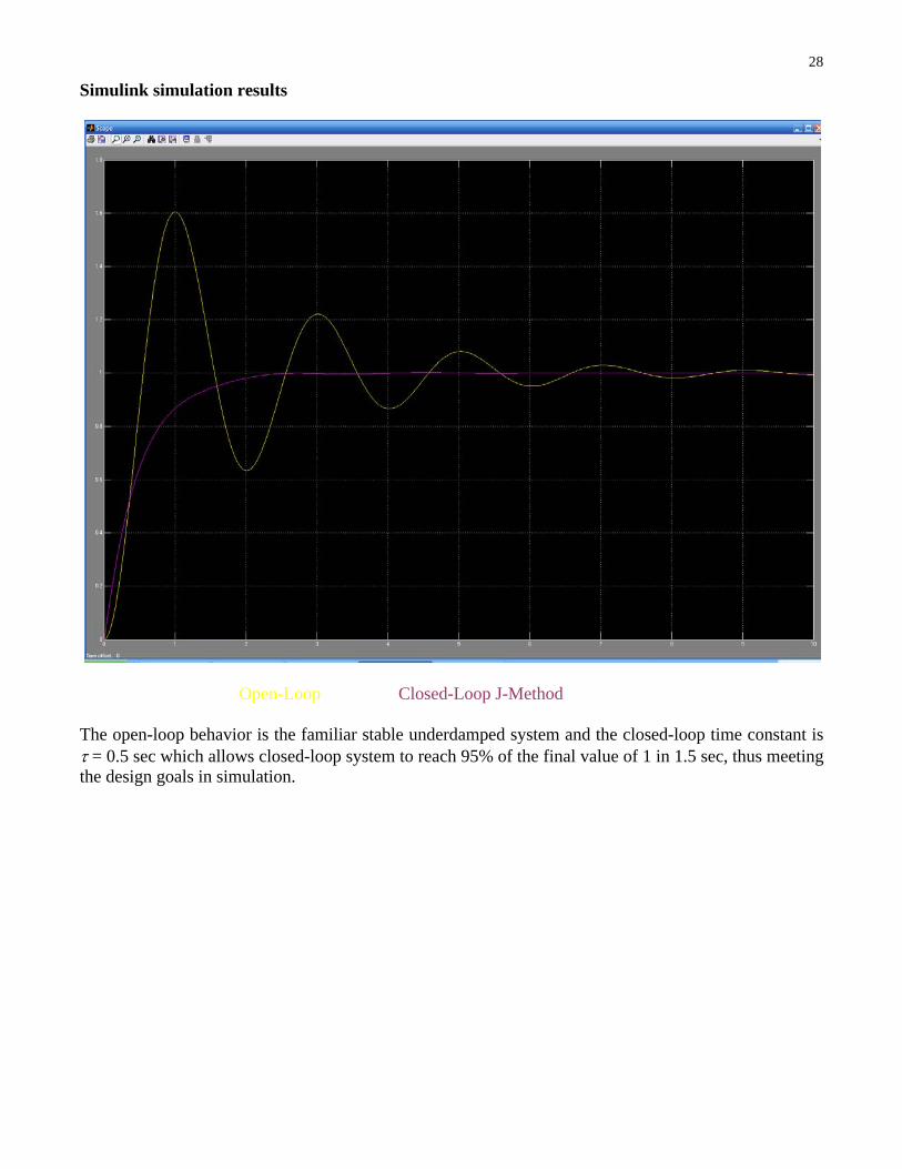
Simulink simulation results
Open-Loop Closed-Loop J-Method
The open-loop behavior is the familiar stable underdamped system and the closed-loop time constant is = 0.5 sec which allows closed-loop system to reach 95% of the final value of 1 in 1.5 sec, thus meeting the design goals in simulation.

29
Examples Summary Table For the combinations of examples considered, the table below summarizes the numerator and denominator orders using the J-Method. Also given is the resulting form of the controller transfer function GC(s) (n.r.f. stands for ‘no recognizable form’).
T(s) a. 1st-order b. 2nd-order c. 3rd-order G(s)
1st
st
st
1
1, PI
st
nd
1
2, Lead/I
st
rd
1
3, n.r.f.
2nd
nd
st
2
1, PID 1
nd
nd
2
2, n.r.f.
nd
rd
2
3, n.r.f.
3rd
rd
st
3
1, n.r.f. 2
rd
nd
3
2, n.r.f. 2
rd
rd
3
3, n.r.f.
Examples GC(s) Summary For the nine example combinations considered, the table below summarizes the resulting controller transfer functions GC(s) using the J-Method.
T(s) a. 1st-order b. 2nd-order c. 3rd-order G(s)
1st
2( 1)s
s
15( 1)
( 6)
s
s s
2
450( 1)
( 36 195)
s
s s s
2nd
2 10
5
s s
s
1
21.5( 10)
( 6)
s s
s s
2
2
45( 10)
( 36 195)
s s
s s s
3rd
3 22 11 10
5
s s s
s
2
3 21.5( 2 11 10)
( 6)
s s s
s s
2
3 2
2
45( 2 11 10)
( 36 195)
s s s
s s s
1Exception to the rule that the order of the denominator of your desired T(s) must be equal or greater than the order of the denominator of G(s). 2Impossible to implement.

30
In addition to this set of nine examples, the J-Method has been successfully tested with the following (where the a-c cases represent the same desired closed-loop transfer functions as above).
Integrating open-loop transfer function G(s) (an s can be factored out in the denominator, i.e. there is no ‘spring’). This is called a Type I system since there is one integrator in the denominator of G(s), as explained in Section 4.5 of the ME 3012 NotesBook.
2
10 10( )
( 1)G s
s s s s
a. 1
( )5C
sG s
b.
1.5( 1)( )
( 6)C
sG s
s
c.
2
45( 1)( )
36 195C
sG s
s s
PD Lead n.r.f.
Non-ideal sensor transfer function ( ) 1H s 1
( )4
H ss
for 1
( )1
G ss
a. 2
2
2( 5 4)( )
6 6C
s sG s
s s
b.
2
3 2
15( 5 4)( )
10 39 45C
s sG s
s s s
c.
2
4 3 2
450( 5 4)( )
40 339 1230 1350C
s sG s
s s s s
Open-loop transfer function G(s) with a zero
2
10( 1)( )
10
sG s
s s
a. 2 10
( )5 ( 1)C
s sG s
s s
b.
2
2
1.5( 10)( )
( 7 6)C
s sG s
s s s
c.
2
3 2
45( 10)( )
( 37 231 195)C
s sG s
s s s s
Unstable open-loop transfer function G(s), e.g. Controller Design Example 2
2
10( )
10G s
s s
a. 2 10
( )5C
s sG s
s
b.
21.5( 10)( )
( 6)C
s sG s
s s
c.
2
2
45( 10)( )
( 36 195)C
s sG s
s s s
Try all of these in Simulink simulation to evaluate their performance.
All examples work as desired – except for the unstable cases which all have numerical instability problems, with the negative KP gains – the unstable poles cannot be cancelled perfectly. So we CANNOT use the J-Method for unstable open-loop systems.

31
Note that the full-T(s)-matching J-Method does not experience any problems with handling open-loop G(s) models with zeroes or higher-order systems. The J-Method controller includes its own internal pre-filter, identical to the one presented in Section 5.9.
Also, problems of denominator parameter matching with higher-order and lower-order systems as exposed in Section 5.10 of the ME 3012 NotesBook are not a problem for the J-Method. J-Method Controller Input Effort For Controller Design Example 1, we first present the output unit step response, followed by the input effort plot, both in comparison to the open-loop case.
Output Unit Step Responses
Open-loop, J-Method Controller

32
J-Controller Input Effort
Open-loop (1), J-Method Controller (1.5)
The J-Method requires no pre-filter – its maximum input effort requirement is 1.5 actuator input units. The J-Method controller does not require a steep rate of change for the actuator input effort.

33
J-Method Controller Disturbance Evaluation Again for Controller Design Example 1, we now present how well the J-Method rejects disturbances.
J-Method, disturbed J-Method A unit step disturbance was turned on at t = 1 sec. Clearly the J-Method controller is very poor at rejecting the disturbance in this example. The disturbed J-Method controller overshoots relatively high, with poor transient dynamics. This disturbed response is heading towards zero steady-state error, however, given enough time.
The PID controller disturbance rejection presented in Section 5.12 of the ME 3012 NotesBook is much better than that of the Lead or J-Method controllers in this example. The PID controller was not designed for disturbance rejection, it just handles the disturbances better.

34
5.14 Term Example Controller Design Open-loop system physical diagram
We will design a controller to control the load angular velocity L(t). Assume a perfect tachometer sensor, H(s) = Kt = 1, so there is negative unity feedback. Note that G2(s) = KT, the motor torque constant, is different from H(s) = Kt, the feedback sensor (tachometer) constant. Here are the open- and closed-loop feedback control system diagrams.
Term Example Open-Loop Diagram
Term Example Closed-Loop Diagram
where 1
1( )G s
Ls R
2 ( ) TG s K
3
1( )
E E
G sJ s c
H(s) = Kt = 1
J M
cM
J (t)L
cL
n
v (t)A
i (t)A
v (t)B
+
-
+
-
L R
L
L
L
(t)
(t)(t)
M
M
M
(t)
(t)(t)
-G (s)1 G (s)3 1/nG (s)2
K B
V (s)A I (s)A T (s)M(s)M (s)L
-G (s)1 G (s)3 1/nG (s)2
K B
V (s)A I (s)A T (s)M(s)M (s)L
-
(s)LDES
K t

35
Step 1. Analyze the as-given open-loop system behavior. Earlier the open-loop transfer function was derived and the real-world parameters for the NASA ARMII robot shoulder joint were substituted.
2
( ) 5( )
( ) 11 1010
T
L
A E E T B
Ks nG s
V s Ls R J s c K K s s
2 2 22 11 1010OL n ns s s s s
1010 31.8n rad/sec 11 110.173
2 2 1010n
1,2 5.5 31.3s i
tR = 0.04 sec tP = 0.10 sec PO = 57.6% tS = 0.71 sec
This open-loop system has a different time scale than Controller Design Example 1; its output
L(t) rises much faster in response to a unit step input vA(t). Also, the steady-state value is 5/1010, whereas it was 1.0 for Controller Design Example 1.

36
First, take a look at the root-locus plots and unit step responses, for the proportional controller GC(s) = K, first for angular velocity output.
Term Example, L(t) control, unit step responses as K increases from 0.
K values legend 0 52 96
179 334 622
-50 0 50-50
-40
-30
-20
-10
0
10
20
30
40
50
Re
Im
L Root Locus
0 0.1 0.2 0.3 0.4 0.5 0.6 0.7 0.8 0.9 10
0.2
0.4
0.6
0.8
1
1.2
1.4
1.6Step Response
Time (sec)
Am
plitu
de
0 0.1 0.2 0.3 0.4 0.5 0.6 0.7 0.8 0.9 10
0.2
0.4
0.6
0.8
1
1.2
1.4
1.6Step Response
Time (sec)
Am
plitu
de
0 0.1 0.2 0.3 0.4 0.5 0.6 0.7 0.8 0.9 10
0.2
0.4
0.6
0.8
1
1.2
1.4
1.6Step Response
Time (sec)
Am
plitu
de
0 0.1 0.2 0.3 0.4 0.5 0.6 0.7 0.8 0.9 10
0.2
0.4
0.6
0.8
1
1.2
1.4
1.6Step Response
Time (sec)
Am
plitu
de
0 0.1 0.2 0.3 0.4 0.5 0.6 0.7 0.8 0.9 10
0.2
0.4
0.6
0.8
1
1.2
1.4
1.6Step Response
Time (sec)
Am
plitu
de
0 0.1 0.2 0.3 0.4 0.5 0.6 0.7 0.8 0.9 10
0.2
0.4
0.6
0.8
1
1.2
1.4
1.6Step Response
Time (sec)
Am
plitu
de

37
Here are the root-locus plot and unit step responses, for the proportional controller GC(s) = K, for angle.
Term Example, L(t) control, unit step responses as K increases from 0.
K values legend 0 20 117
681 2220 3955
9529 55309 220190
The closed-loop system becomes unstable for 2222K ! Clearly the simple proportional controller will not work, since the angular velocity root-locus plot shows that the closed-loop dimensionless damping ratio must decrease as K increases.
-50 0 50-50
-40
-30
-20
-10
0
10
20
30
40
50
Re
Im
L Root Locus
0 0.2 0.4 0.6 0.8 1-1
-0.5
0
0.5
1Step Response
Time (sec)
Am
plitu
de
0 0.2 0.4 0.6 0.8 10
0.02
0.04
0.06
0.08
0.1Step Response
Time (sec)
Am
plitu
de
0 0.2 0.4 0.6 0.8 10
0.1
0.2
0.3
0.4
0.5Step Response
Time (sec)A
mpl
itude
0 0.2 0.4 0.6 0.8 10
0.2
0.4
0.6
0.8
1Step Response
Time (sec)
Am
plitu
de
0 0.2 0.4 0.6 0.8 10
0.5
1
1.5
2Step Response
Time (sec)
Am
plitu
de
0 0.2 0.4 0.6 0.8 1-10
-5
0
5
10Step Response
Time (sec)
Am
plitu
de
0 0.2 0.4 0.6 0.8 1-1
-0.5
0
0.5
1x 10
4 Step Response
Time (sec)
Am
plitu
de
0 0.2 0.4 0.6 0.8 1-2
-1.5
-1
-0.5
0
0.5
1
1.5
2x 10
11 Step Response
Time (sec)
Am
plitu
de
0 0.2 0.4 0.6 0.8 1-1
-0.5
0
0.5
1x 10
20 Step Response
Time (sec)
Am
plitu
de
38
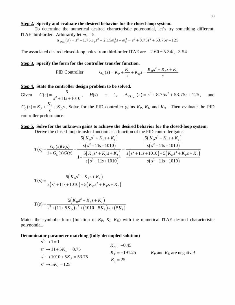
Step 2. Specify and evaluate the desired behavior for the closed-loop system. To determine the numerical desired characteristic polynomial, let’s try something different: ITAE third-order. Arbitrarily let n = 5.
3 2 2 3 3 2( ) 1.75 2.15 8.75 53.75 125DES n n ns s s s s s s
The associated desired closed-loop poles from third-order ITAE are 2.60 5.34 , 3.54i . Step 3. Specify the form for the controller transfer function.
PID Controller 2
( ) I D P IC P D
K K s K s KG s K K s
s s
Step 4. State the controller design problem to be solved.
Given 2
5( )
11 1010G s
s s
, H(s) = 1, 3 2( ) 8.75 53.75 125
DESCL s s s s , and
( ) IC P D
KG s K K s
s , Solve for the PID controller gains KP, KI, and KD. Then evaluate the PID
controller performance. Step 5. Solve for the unknown gains to achieve the desired behavior for the closed-loop system.
Derive the closed-loop transfer function as a function of the PID controller gains.
2 2
2 2
2 2 2
2 2
2
2 2
2
3
5 5
11 1010 11 1010( ) ( )( )
1 ( ) ( ) 5 11 1010 51
11 1010 11 1010
5( )
11 1010 5
5( )
D P I D P I
C
C D P I D P I
D P I
D P I
D P I
K s K s K K s K s K
s s s s s sG s G sT s
G s G s K s K s K s s s K s K s K
s s s s s s
K s K s KT s
s s s K s K s K
K s K s KT s
s
211 5 1010 5 5D P IK s K s K
Match the symbolic form (function of KP, KI, KD) with the numerical ITAE desired characteristic polynomial. Denominator parameter matching (fully-decoupled solution)
3
2
1
0
1 1
11 5 8.75
1010 5 53.75
5 125
D
P
I
s
s K
s K
s K
0.45
191.25
25
D
P
I
K
K
K
KP and KD are negative!

39
Step 6. Evaluate the PID controller performance in simulation. Open- vs. Closed-Loop unit step responses
Open-Loop Open-Loop Closed-Loop PID Closed-Loop PID, corrected
Step 7. Include an output attenuation correction factor if necessary. Here the KI term forces the steady-state output to 1.0 (zero steady-state error for unit step input); however, the original system output was not 1.0 (it was 5/1010, we can’t even see it on the graph), so we need a correction factor to drive the closed-loop system to the same steady-state value (right plot).
5 1010( ) ( )( ) ( ) ( ) 0.00495 ( )
1sso
corrssc
yR s R s corr R s R s R s
y
Corrected closed-loop PID transfer function 2
3 2
5 2.25 956.25 125( )
1010 8.75 53.75 125
s sT s
s s s
Again: Controller design can easily make matters worse, if not done properly! With negative KP, the closed-loop step response initially goes down while open-loop goes up. The is a huge (negative) overshoot, and the transient response is slower than the open-loop case. Step 9. Re-design and re-evaluate the controller.
Perform design iteration until the closed-loop performance specifications are met in simulation. We have no pre-filter yet (Step 8), but we have a bigger problem in the negative KP and KD. Step 2. Specify and evaluate the desired behavior for the closed-loop system. So let’s choose a higher n in the third-order ITAE desired closed-loop numerical characteristic polynomial for faster response and positive KP, KD. KP is the limiting case, i.e. if we force it to be positive, KD will be positive also.
11 5 1.75D nK
@ KD = 0, n = 6.29, but then KP will still be negative (KP = –185); therefore let us instead set n so that KP will be positive.
21010 5 2.15P nK @ KP = 0, n = 21.7
So try n = 30 3 2( ) 52.5 1935 27000DES s s s s
0 0.5 1 1.5 2 2.5 3-16
-14
-12
-10
-8
-6
-4
-2
0
2
4
L(t
)
t (sec)0 0.5 1 1.5 2 2.5 3
-0.08
-0.07
-0.06
-0.05
-0.04
-0.03
-0.02
-0.01
0
0.01
0.02
L(t
)
t (sec)
40
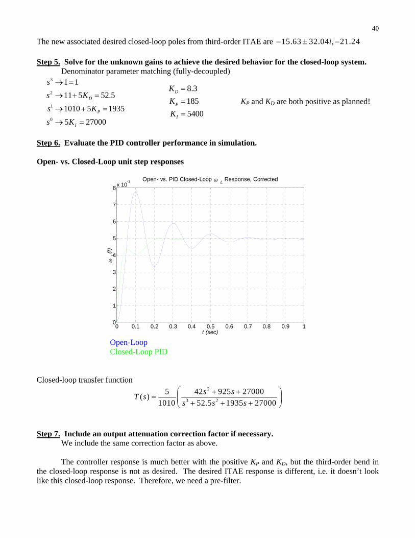
The new associated desired closed-loop poles from third-order ITAE are 15.63 32.04 , 21.24i
Step 5. Solve for the unknown gains to achieve the desired behavior for the closed-loop system. Denominator parameter matching (fully-decoupled)
3
2
1
0
1 1
11 5 52.5
1010 5 1935
5 27000
D
P
I
s
s K
s K
s K
8.3
185
5400
D
P
I
K
K
K
KP and KD are both positive as planned!
Step 6. Evaluate the PID controller performance in simulation. Open- vs. Closed-Loop unit step responses
Open-Loop Closed-Loop PID
Closed-loop transfer function
2
3 2
5 42 925 27000( )
1010 52.5 1935 27000
s sT s
s s s
Step 7. Include an output attenuation correction factor if necessary.
We include the same correction factor as above. The controller response is much better with the positive KP and KD, but the third-order bend in the closed-loop response is not as desired. The desired ITAE response is different, i.e. it doesn’t look like this closed-loop response. Therefore, we need a pre-filter.
0 0.1 0.2 0.3 0.4 0.5 0.6 0.7 0.8 0.9 10
1
2
3
4
5
6
7
8x 10
-3
L(t
)
t (sec)
Open- vs. PID Closed-Loop L Response, Corrected

41
Step 8. Include a pre-filter transfer function if necessary.
Two unwanted zeroes were introduced by the PID controller; these can be cancelled by a pre-filter.
Pre-filter transfer function 2
27000( )
42 925 27000PG ss s
Note we specify the 27000 pre-filter transfer function numerator since the pre-filter shouldn’t attenuate the output. When we plot the resulting unit step responses we see in the left plot below that the controller design is now successful.
Open-Loop Closed-Loop PID Closed-Loop PID with Pre-Filter
The pre-filtered closed-loop transfer function is:
3 2
5 27000( )
1010 52.5 1935 27000T s
s s s
The final closed-loop unit step response is now theoretically identical to the specified third-order
ITAE behavior. Note with the ITAE specification we didn’t need to specify percent overshoot, settling time, or peak time.
For this controller, the angle L(t) unit step response in time is given in the right plot above (note the steady-state error since the closed-loop PID lags the open-loop and the closed-loop PID with pre-filter lags even further). We just integrated the L(t) response to get these results, i.e. we included another s factor in the closed-loop system denominator.
0 0.1 0.2 0.3 0.4 0.5 0.6 0.7 0.8 0.9 10
1
2
3
4
5
6
7
8x 10
-3
L(t
)
t (sec)
Open-, PID Closed-, and Pre-filtered L Response
0 0.1 0.2 0.3 0.4 0.5 0.6 0.7 0.8 0.9 10
0.5
1
1.5
2
2.5
3
3.5
4
4.5
5x 10
-3
L(t
)
t (sec)
Open-, PID Closed-, and Pre-filtered L Response

42
Step 6. Evaluate the PID controller performance in simulation. Simulink Model
The Plant blocks above are Simulink masks for the (identical) open-loop plant shown below.
V
ThetaL
ReferenceOmegaL
27000
42s +925s+270002
Pre-fi lter Plant
Plant
PID
PID Controller
OmegaL
1s
Integrator2
1s
Integrator
-K-
Corr
1
out_1
tau dist
1
s+10
RL Circuit
100
Km
1
Kb
1
0.1s+0.1
Jc rotational dynamics
-K-
1/n
1
in_1

43
J-Method Controller Alternate design method for Term Example L(t) controller design. Step 2. Specify the desired behavior for the closed-loop system We specify the entire desired closed-loop T(s), not just the denominator. To determine the numerical desired entire closed-loop T(s) transfer function, let’s try something different: ITAE second-order.
2 2
2
( ) 1.4
( ) 42 900
DES n n
DES
s s s
s s s
n = 30 (from successful PID controller design)
The associated desired closed-loop poles from third-order ITAE are 2 1 2 1 .4 i .
2
5(900)1010( )42 900
T ss s
Step 4. Solve for the unknown controller form including the unknown gains. J-Method
( )
( )( ) 1 ( ) ( )C
T sG s
G s H s T s
with 2
5( )
11 1010G s
s s
and H(s) = 1
2
2 2
2
2
2
2
2
2
5(900)101042 900( )
5(900)5 10101 (1)
11 1010 42 900
45011 1010101
42 900 5
( )450
42 900101
42 900
9011 1010
101( )42 450 2
C
C
C
s sG s
s s s s
s ss s
G ss s
s s
s sG s
s s
1
101

44
Step 5. Simulate the resulting closed-loop system performance. Simulink Evaluation for the J-Method Term Example Controller Design, Angular Velocity
Open-Loop Closed-Loop J-Method
StepScope
5
s +11s+10102
Plant
5
s +11s+10102
Plant
s +42s+450*(2-1/101)2
90/101*[1 11 1010]
Gc

45
Open-Loop Closed-Loop J-Method Disturbed Closed-Loop J-Method There is no need for a correction factor or a pre-filter transfer function. This J-Method controller for the Term Example load shaft angular velocity L(t) control was successful as shown in the left plot above. But how does this controller handle disturbances?
As we have seen before, the J-Method controller is very poor at handling disturbances, in this case a unit step disturbance in voltage, subtracted at t = 1 sec. The disturbed J-Method controller output response, shown in the right figure above, has unacceptable transient response and unacceptable steady-state error.

46
5.15 Term Example Disturbances and Steady-State Error
Though we have not presented it, it is possible to design controllers specifically to reject disturbances. This last example, the conclusion of the Term Example, discusses controller design to reject disturbances, specifically for achieving lower steady-state error. Term Example open-loop diagram with disturbance
where VA(s) is the armature voltage input, L(s) is the load shaft angular velocity output, and D(s) is the disturbance modeled at the actuator input level (disturbance in torque, Nm).
where 1
1( )G s
Ls R
2 ( ) TG s K 3
1( )
E E
G sJ s c
Let VA(s) = 0 and monitor changes in L(s) given a disturbance input. Since VA(s) = 0, any L(s) is the steady-state error, that is, we wish as low an output as possible for the open-loop system.
Derive the open-loop disturbance transfer function ( )
( )( )
LD
sG s
D s
.
( ) 1
( ) ( )M
M E E
s
T s D s J s c
J M
cM
J (t)L
cL
n
v (t)A
i (t)A
v (t)B
+
-
+
-
L R
L
L
L
(t)
(t)(t)
M
M
M
(t)
(t)(t)
-G (s)1 G (s)3 1/nG (s)2
K B
V (s)A I (s)A T (s)M(s)M (s)L
D(s)

47
Since V(s) = 0 ( )
( )M T
B M
T s K
K s Ls R
( ) ( )M Ls n s
( ) 1( )
( )
L
T B L E E
n sK K n s J s cD s
Ls R
( ) ( )( ) T B L
L E E
K K n s Ls R D sn s J s c
Ls R
( ) ( )E E T B Ln J s c Ls R nK K s Ls R D s
( )( )
( )L
DE E T B
Ls RsG s
D s n J s c Ls R K K
Open-loop steady-state error for a step disturbance of magnitude D, ( )D
D ss
( ) ( ) ( ) ( ) ( )OL LDES L L
E E T B
Ls RE s s s s D s
n J s c Ls R K K
lim ( ) lim ( ) lim0 0ssOL OL OL
E E T B
ssOLE T B
Ls R De e t sE s s
t s s sn J s c Ls R K K
RDe
n RC K K
Closed-loop diagram with disturbance, tachometer, and P controller
where LDES(s) is the desired load shaft angular velocity output, and the other terms have been previously defined.
-G (s)1 G (s)3 1/nG (s)2
K B
V (s)A I (s)A T (s)M(s)M (s)L
D(s)
-
(s)LDES
K t

48
Let LDES(s) = 0 and check changes in L(s) given a disturbance input. Since LDES(s) = 0, any L(s) is the steady-state error, that is, we wish as low an output as possible for the closed-loop system.
Derive the closed-loop disturbance transfer function ( )
( )( )
LD
LDES
sT s
s
.
( ) 1
( ) ( )M
M D E E
s
T s T s J s c
( )
( )M TT s K
A s Ls R
( ) ( )M Ls n s
( ) ( ) ( )
( ) ( ) ( ) ( ) ( )
( ) ( ) ( ) ( )
A B M
A CL LDES t L t L
t L B L t B L
A s V s K s
V s KE s K s K s KK s
A s KK s nK s KK nK s
( )
( ) T t B LM
K KK nK sT s
Ls R
( ) 1
( )( )
L
T t B L E E
n sK KK nK s J s c
D sLs R
( ) ( )( ) T t B L
L E E
K KK nK s Ls R D sn s J s c
Ls R
( ) ( )E E T t B Ln J s c Ls R K KK nK s Ls R D s
( )
( )( )
LD
LDES E E T t B
Ls RsT s
s n J s c Ls R K KK nK
Closed-loop steady-state error for a step disturbance of magnitude D, ( )D
D ss
( ) ( ) ( ) ( )CL LDES L LE s s s s
( ) ( )CL
E E T t B
Ls RE s D s
n J s c Ls R K KK nK
lim ( ) lim ( )
0ssCL CL CLe e t sE st s
lim
0ssCL
E E T t B
Ls R De s
s sn J s c Ls R K KK nK

49
ssCLE T t B
RDe
nRc K KK nK
For disturbance-rejecting controller design, ensure the closed-loop steady-state error is less than the open-loop steady-state error.
E T BssCL
ssOL E T t B
E T BssCL
ssOL E T t B
n Rc K Ke RD
e nRc K KK nK RD
n Rc K Ke
e nRc K KK nK
Design so 1ssCL
ssOL
e
e

50
Numerical example from Term Example
10
200 1 100
10
20200
ssOLE T B
RDe
n Rc K K
D
D
10
200 100 200
10
20200 100
ssCLE T t B
t
t
RDe
nRc K KK nK
D
KK
D
KK
10 20200
20200 100 10
20200
20200 100
ssCL
ssOL t
t
e D
e KK D
KK
20200
120200 100
ssCL
ssOL t
e
e KK
20200 100 20200
100 0
0
t
t
t
KK
KK
KK
Kt tachometer selection K proportional controller gain Assume the tachometer gain is fixed. Then the only way to reduce the closed-loop steady-state error is to increase proportional controller gain K as much as possible. Now, this proportional controller for disturbance rejection is not very satisfying – we know from the root-locus plot that the higher we make K, the worse the transient response will be (stable but more highly underdamped as K increases). So this demonstrates another tradeoff in controller design – to ensure lower steady-state errors due to unknown, unwanted disturbances, we must accept worse transient response performance.

51
6. Vibrational Responses
6.1 Free Vibrational Responses 6.1.1 Undamped Second-Order System Free Responses: Simple Harmonic Motion 6.1.1.1 Analytical Undamped Second-Order System Free ODE Solutions Analytical Solution via the Laplace Transform Method Let us solve the same general unforced Harmonic Oscillator second-order IVP ODE using an alternative method: Laplace Transforms. Since we are solving a linear ODE, there is a unique solution, which we have found using the Slow ME Way and validated by direct substitution. The Problem Statement is the same:
Solve 2 0( ) ( ) 0a x t a x t for x(t) given a2, a0, and values for the initial conditions:
0
0
(0)
(0)
x x
x v
In contrast to the Slow ME Way, ODE solution via Laplace Transforms is accomplished algebraically in the Laplace frequency domain, in a single step, including the initial conditions. The first step is to take the Laplace Transform of both sides of the ODE, including the initial conditions, and solving algebraically for the unknown in the Laplace domain, ( ) { ( )}X s L x t .
2 0
22 0
22 0 2 0 0
2 0 02
2 0
( ) ( ) 0
( ( ) (0) (0)) ( ) 0
( ) ( ) ( )
( )( )
L a x t a x t
a s X s sx x a X s
a s a X s a x s v
a x s vX s
a s a
Note that the system characteristic polynomial 2
2 0a s a appears when using the Laplace
Transform method. To find the solution in the time domain, x(t), we must take the inverse Laplace Transform of X(s).
52
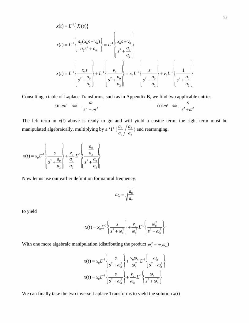
1
1 12 0 0 0 02
2 02 0
2
1 1 1 10 00 0
2 2 2 20 0 0 0
2 2 2 2
( ) ( )
( )( )
1( )
x t L X s
a x s v x s vx t L L
aa s a sa
x s v sx t L L x L v L
a a a as s s s
a a a a
Consulting a table of Laplace Transforms, such as in Appendix B, we find two applicable entries.
2 2sin t
s
2 2
coss
ts
The left term in x(t) above is ready to go and will yield a cosine term; the right term must be
manipulated algebraically, multiplying by a ‘1’ ( 0 0
2 2
a a
a a) and rearranging.
0
1 10 20
2 20 0 0
2 2 2
( )
av as
x t x L La a a
s sa a a
Now let us use our earlier definition for natural frequency:
0
2n
a
a
to yield
21 10
0 2 2 2 2 2( ) n
n n n
vsx t x L L
s s
With one more algebraic manipulation (distributing the product 2
n n n )
1 100 2 2 2 2 2
1 100 2 2 2 2
( )
( )
n n
n n n
n
n n n
vsx t x L L
s s
vsx t x L L
s s
We can finally take the two inverse Laplace Transforms to yield the solution x(t)

53
00( ) cos sinn n
n
vx t x t t
As predicted, this solution agrees with the solution derived via the Slow ME Way – we have validated this solution, presented some equivalent alternative solution forms, and presented a numerical example so we needn’t repeat this work since it is the same.

54
6.1.2 Underdamped Second-Order System Free Responses 6.1.2.4 Damped Second-Order System Free Response Numerical ODE Solutions Numerical Plots with All Three Derivatives For a more complete graphical result in this numerical example, we next separately plot on the next four graphs, the same displacements x(t) as above, along with two derivatives. The first one, for undamped free SHM using MATLAB file SHM.m, has been presented previously.
( ) 0.0100cos 0.0095sin
( ) 0.0314sin 0.0300cos
( ) 0.0987 cos 0.0942sin
x t t t
x t t t
x t t t
Undamped SHM Numerical Example x(t) and Time Derivatives Time Response

55
Underdamped SHM Numerical Example x(t) and Time Derivatives Time Response
Critically-damped SHM Numerical Example x(t) and Time Derivatives Time Response
Overdamped SHM Numerical Example x(t) and Time Derivatives Time Response
Note that if n > 1 then the magnitude of the acceleration is greater than the magnitude of the velocity, which is greater than the magnitude of the position, in all four cases. The previous three plots were generated by MATLAB file DO.m.

56
6.2 Forced Vibrational Responses Analytical Solution via the Laplace Transform Method Let us solve the same general harmonically-forced undamped second-order IVP ODE using an alternative method: Laplace Transforms. Since we are solving a linear ODE, there is a unique solution, which we have found using the Slow ME Way and validated by direct substitution. The Problem Statement is the same:
Solve 2 0( ) ( ) ( )a x t a x t u t for x(t) given a2, a0, ( ) sinu t U t , and zero initial conditions
0
0
(0) 0
(0) 0
x x
x v
In contrast to the Slow ME Way, ODE solution via Laplace Transforms is accomplished algebraically in the Laplace frequency domain, in a single step, including the forcing function and initial conditions. The first step is to take the Laplace Transform of both sides of the ODE, including the initial conditions and forcing function, and solving algebraically for the unknown in the Laplace domain,
( ) { ( )}X s L x t .
2 0
22 0 2 2
22 0 2 2
2 2 22 0
( ) ( ) sin
( ( ) (0) (0)) ( )
( ) ( )
( )( )( )
L a x t a x t U t
a s X s sx x a X s Us
a s a X s Us
UX s
a s a s
Note that the system characteristic polynomial 2
2 0a s a appears when using the Laplace
Transform method. To find the solution in the time domain, x(t), we must take the inverse Laplace Transform of X(s).
1
12 2 2
2 0
( ) ( )
( )( )( )
x t L X s
Ux t L
a s a s
We find no Laplace Transform entries matching this X(s), so we must first perform the Heaviside Partial Fraction Expansion on X(s) to break it into manageable pieces that are found in the Laplace Transform Table.
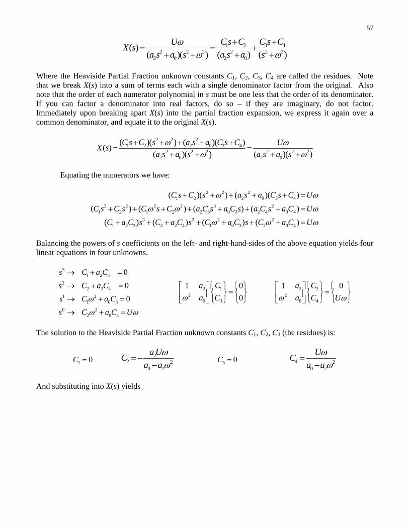
57
3 41 22 2 2 2 2 2
2 0 2 0
( )( )( ) ( ) ( )
C s CCs CUX s
a s a s a s a s
Where the Heaviside Partial Fraction unknown constants C1, C2, C3, C4 are called the residues. Note that we break X(s) into a sum of terms each with a single denominator factor from the original. Also note that the order of each numerator polynomial in s must be one less that the order of its denominator. If you can factor a denominator into real factors, do so – if they are imaginary, do not factor. Immediately upon breaking apart X(s) into the partial fraction expansion, we express it again over a common denominator, and equate it to the original X(s).
2 2 21 2 2 0 3 4
2 2 2 2 2 22 0 2 0
( )( ) ( )( )( )
( )( ) ( )( )
C s C s a s a C s C UX s
a s a s a s a s
Equating the numerators we have:
2 2 2
1 2 2 0 3 4
3 2 2 2 3 21 2 1 2 2 3 0 3 2 4 0 4
3 2 2 21 2 3 2 2 4 1 0 3 2 0 4
( )( ) ( )( )
( ) ( ) ( ) ( )
( ) ( ) ( ) ( )
C s C s a s a C s C U
C s C s C s C a C s a C s a C s a C U
C a C s C a C s C a C s C a C U
Balancing the powers of s coefficients on the left- and right-hand-sides of the above equation yields four linear equations in four unknowns.
31 2 3
22 2 4
1 21 0 3
0 22 0 4
0
0
0
s C a C
s C a C
s C a C
s C a C U
2 12
0 3
1 0
0
a C
a C
2 22
0 4
1 0a C
a C U
The solution to the Heaviside Partial Fraction unknown constants C1, C2, C3 (the residues) is:
1 0C
22 2
0 2
a UC
a a
3 0C
4 20 2
UC
a a
And substituting into X(s) yields

58
3 41 22 2 2
2 0
2 4 22 2 2 2 2 2 2 2
2 0 0 2 2 0 0 2
0
22 2 2 2 2 2
2 20 2 0 20 00
2 22
( )( ) ( )
1 1( )
( ) ( ) ( ) ( )
1( )
( ) ( )
C s CC s CX s
a s a s
C C a U UX s
a s a s a a a s a a a s
a
aU UX s
a a s a a sa aas s
a aa
Consulting a table of Laplace Transforms, such as in Appendix B, we find an applicable entry.
2 2sin t
s
0
21 12 2 2
20 2 00
22
20 2
( ) ( )( )
( ) sin sinnn
a
aUx t L X s L
a a saas
aa
Ux t t t
a a
where 0
2n
a
a
As predicted, this solution agrees with the solution derived via the Slow ME Way – we have validated this solution and presented a numerical example so we needn’t repeat this work since it is the same.

59
6.2.2 Damped Second-Order System Harmonically-Forced Responses
6.2.2.2 Damped Second-Order System Harmonically-Forced Numerical Examples
a. Critically-damped Solution 1
characteristic polynomial 2 22s s
roots ,
2
62.831
2 2 100
c
km
( ) (0.0000192 0.002 ) 0.0000779sin(8 2.89)tx t t e t
2 2 1
sec8 4
T
As seen in the time response plot below for the total x(t), one steady-state mode of vibration is superimposed onto the non-oscillatory critically-damped transient response. We see that the transient response disappears (the total solution approaches the steady-state solution) by around 3 sec. The particular solution remains for as long as the input harmonic forcing function is applied. At t = 0, the initial value is 0 m and the slope is also zero, as specified by the zero initial conditions.
Harmonically-Forced Critically-Damped Numerical Example x(t) Time Response

60
Below we plot the same x(t) response for the same example as the above plot, along with its first and second derivatives. These three are arranged separately on a subplot since their magnitudes are greatly different; the acceleration is the largest, then the velocity, and the position magnitudes are the smallest. We see that the acceleration reaches steady-state before the velocity, which reaches steady-state before the position. We see both initial conditions, i.e. zero initial position and velocity. It also turns out that the initial acceleration is zero, though this is not specified since it is only a second-order problem. What are the relationships amongst these plots, from Calculus?
Same Critically-Damped Numerical Example with Position Velocity, and Acceleration

61
Now we plot the same response for the same example as the above two plots, this time showing the ( )x t vs. x(t) phase plot. To emphasize the steady-state behavior (vibratory response to the harmonic forcing function), the plot below includes time up to 20 sec, instead of 6 sec as before. How do we interpret this complicated graph? Where is time on this graph?
Same Critically-Damped Numerical Example, Phase Plot

62
Let us repeat the above critically-damped numerical example, only changing the driving frequency , with associated driven time period T 16x longer.
( ) sin 0.5sin2
f t F t t
2 24 sec
2
T
The new time response is plotted below.
Harmonically-Forced Critically-Damped Example x(t) Time Response with Lower The natural frequency n is unchanged and the new second-order response x(t) is:
210 rad
10 secn
( ) (0.0032 0.0064 ) 0.0041sin( 0.93)2
tx t t e t
Again in the total time response x(t), one steady-state mode of vibration is superimposed onto the non-oscillatory critically-damped transient response. We see that the transient response again disappears (the total solution approaches the steady-state solution) by around 3 sec. The particular solution remains for as long as the input harmonic forcing function is applied. At t = 0, the initial value is 0 m and the slope is also zero, as specified by the zero initial conditions. The two plots below show the same second critically-damped system harmonically-forced example, first the position, velocity, and acceleration and second the phase plot.

63
Second Critically-Damped Numerical Example with Position Velocity, and Acceleration
Second Critically-Damped Numerical Example, Phase Plot (t = 40 sec)

64
b. Overdamped Solution 1
characteristic polynomial 2 212.57s s
roots –0.84, –11.73
2
125.662
2 2 100
c
km
0.84 11.72( ) 0.000183 0.000150 0.000072sin(8 2.67)t tx t e e t
2 2 1
sec8 4
T
As seen in the time response plot below for the total x(t), one steady-state mode of vibration is superimposed onto the non-oscillatory overdamped transient response. We see that the transient response disappears (the total solution approaches the steady-state solution) by around 6 sec, slower than the critically-damped case. The particular solution remains for as long as the input harmonic forcing function is applied. At t = 0, the initial value is 0 m and the slope is also zero, as specified by the zero initial conditions.
Harmonically-Forced Overdamped Numerical Example x(t) Time Response
65
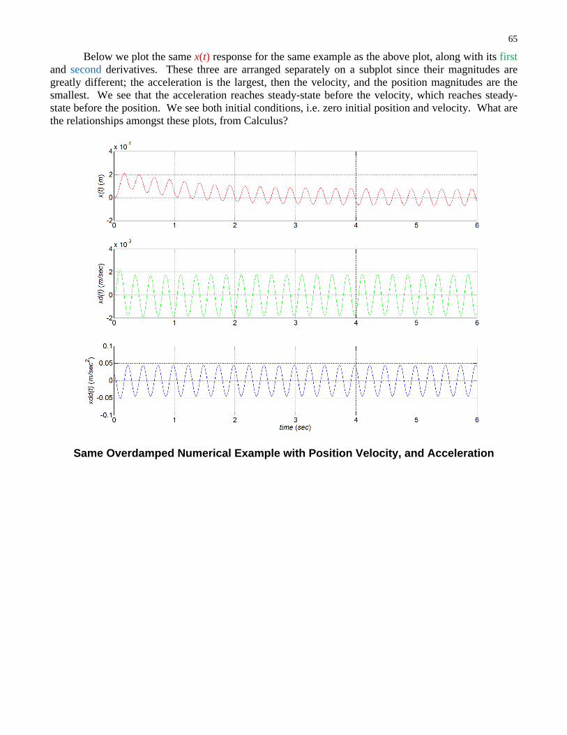
Below we plot the same x(t) response for the same example as the above plot, along with its first and second derivatives. These three are arranged separately on a subplot since their magnitudes are greatly different; the acceleration is the largest, then the velocity, and the position magnitudes are the smallest. We see that the acceleration reaches steady-state before the velocity, which reaches steady-state before the position. We see both initial conditions, i.e. zero initial position and velocity. What are the relationships amongst these plots, from Calculus?
Same Overdamped Numerical Example with Position Velocity, and Acceleration

66
Now we plot the same response for the same example as the above two plots, this time showing the ( )x t vs. x(t) phase plot. To emphasize the steady-state behavior (vibratory response to the harmonic forcing function), the plot below includes time up to 20 sec, instead of 6 sec as before. How do we interpret this complicated graph? Where is time on this graph?
Same Overdamped Numerical Example, Phase Plot
67
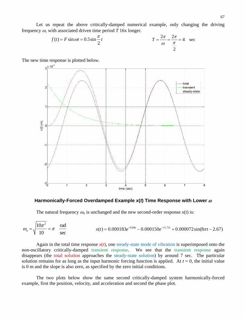
Let us repeat the above critically-damped numerical example, only changing the driving frequency , with associated driven time period T 16x longer.
( ) sin 0.5sin2
f t F t t
2 24 sec
2
T
The new time response is plotted below.
Harmonically-Forced Overdamped Example x(t) Time Response with Lower The natural frequency n is unchanged and the new second-order response x(t) is:
210 rad
10 secn
0.84 11.72( ) 0.000183 0.000150 0.000072sin(8 2.67)t tx t e e t
Again in the total time response x(t), one steady-state mode of vibration is superimposed onto the non-oscillatory critically-damped transient response. We see that the transient response again disappears (the total solution approaches the steady-state solution) by around 7 sec. The particular solution remains for as long as the input harmonic forcing function is applied. At t = 0, the initial value is 0 m and the slope is also zero, as specified by the zero initial conditions. The two plots below show the same second critically-damped system harmonically-forced example, first the position, velocity, and acceleration and second the phase plot.

68
Second Overdamped Numerical Example with Position Velocity, and Acceleration
Second Overdamped Numerical Example, Phase Plot (t = 40 sec)

69
6.2.2.5 Transmissibility An important topic in vibrations and machine design is vibration isolation. For a given machine, designers specify the mountings (combinations of springs and dashpots) to reduce the shaking forces and moments on the ground as much as possible. Passive vibration isolation indicates using fixed components for isolation. Active vibration isolation requires sensors, a processor, actuation, and control theory, which is much more complicated, but with potential improvements in vibration isolation compared to the passive case. Transmissibility is defined as the ratio of the maximum force transmitted to the base over the maximum input force magnitude and is thus unitless or can be expressed as a percentage. In a good vibration isolation system, the transmissibility should be low, much less than 1. Consider the standard forced m-c-k system. Recall from the ME 3012 NotesBook section on resonance that the maximum normalized amplitude M is:
2 2 2
1
(1 ) (2 )
AM
F k r r
n
r
where A is the amplitude of vibration, F is the input sinusoidal force magnitude, and k is the spring constant. In this system the ground force is transmitted through the spring and dashpot elements. Recall that the spring and dashpot forces are ( )Sf kx t and ( )Df cx t . Further recall that the velocity ( )x t always leads the position x(t) by 90 . Therefore the total maximum transmitted force Ft is:
22
22 2 2( ) ( ) 1 1 1 2t
n
cF kA cA kA kA kA r
k
And the transmissibility TR is the ratio of Ft over F.
2
2 2 2
2
2 2 2
1 2
(1 ) (2 )
1 (2 )
(1 ) (2 )
tkA rF
TRF kA r r
rTR
r r
Note that this TR result has the same denominator as the M ratio from the resonance discussion, but a different numerator. Below we plot TR vs. frequency ratio r, for various values.

70
Transmissibility vs. r
We see all curves pass through the same ratio point of 1 at r = 0 and 2r . From these graphical results we see that the designer must keep the frequency ratio r as large as possible and the damping as small as possible to achieve low transmissibility 1TR . MATLAB file Transmiss.m was used to generate the above curves. The vibrational model for a second-order m-c-k system with input displacement u(t) instead of input external force f(t) is:
( ) ( ) ( ) ( ) ( )mx t cx t kx t cu t ku t
Due to the similarity of these models, the transmissibility X
TRU
is identical to the transmissibility
tFTR
F and so the above plot covers the displacement input case also, with the same design
conclusions.

71
6.2.2.6 Rotating Imbalance The model for a machine with a rotating imbalance is shown below.
22 1( ) ( ) ( ) sinm x t cx t kx t m e t
where the unbalanced mass is m1, the total machine mass is m2, e is the effective offset length of the imbalance, and the equivalent spring and damping coefficients connecting the machine to ground are k and c, respectively. Following the same method we used for deriving the resonance plots we obtain the dimensionless ratio E expressing the machine motion relative to the unbalanced motion.
22
2 2 21 (1 ) (2 )
m A rE
m e r r
This E relationship is plotted below vs. frequency ratio r, for various values.
Unbalanced motion ratio vs. r
m1
m2
k c
x(t)
e
t

72
At first this series of plots resembles the resonance plots from before. Two main differences are that the peaks in E ratios for the various values are to the right of r = 1, rather than to the left, and the final value asymptote is 1 rather than 0. This means that the machine vibration approaches that of the rotating imbalance as r increases. Again, r values near resonance are to be avoided due to high output motion. The transmissibility results for this rotating imbalance case are different than for the two cases presented previously in the last section. The transmissibility in this case is defined as the force transmitted to ground through the springs and dashpots, relative to the normalized unbalanced mass.
2 2
2 2 21 2
1 (2 )
(1 ) (2 )t
U
r rF kTR
m e m r r
This TRU relationship is plotted below vs. frequency ratio r, for various values.
Unbalanced transmissibility TRU vs. r
We see all curves pass through the same transmissibility point of 2 at 2r . Again, we desire very low values of transmissibility in the rotating unbalance case, that is we want 1UTR . In
the TRU plots above we see that all cases will yield 1UTR , some even yield 1UTR . For all r
values greater than 1, (and for many r values less than 1), higher damping causes higher transmissibility, which is undesirable. The best way to limit transmissibility in this case is to minimize the rotating imbalance 1m e by balancing the rotating shaft.
MATLAB file Transmiss.m was used to generate the above two plots.

73
6.2.3 General Forcing Functions In forced vibrations analysis we considered only periodic harmonic input forcing of the form
( ) sinf t F t We could have equally considered periodic harmonic input forcing of the form ( ) cosf t F t . All derived results would be very similar so we needn’t repeat our derivations for the cosine input function. This section discusses more general input functions for forced vibrations of dynamic systems. We consider both periodic and non-periodic general input forcing functions. These topics used to be central in learning classical vibrations, but, with the advent of MATLAB/Simulink, these types of general input functions are easy to represent using computer simulation. These simulations are much more accurate and far easier to perform than earlier in history. 6.2.3.1 Periodic Forcing Functions
Periodic forcing functions used as external inputs to vibratory systems have classically been represented by the Fourier series. Any periodic forcing function f(t) with a time period of 2T can be represented by an infinite Fourier series.
0
1 1
( ) cos sin2 p p
p p
af t a p t b p t
where
0
2( )cos
T
pa f t p tdtT
0,1,2,p
0
2( )sin
T
pb f t p tdtT
1,2,p
It is up to the engineer to decide how many p terms to include in the series to obtain the desired fidelity and accuracy. An alternate form for the Fourier series, suitable for the frequency response, is obtained by using a familiar transformation (sine sum-of-angles formula); the result is:
01
( ) sinp pp
f t A A p t
where
00 2
aA
2 2p p pA a b
1tan pp
p
a
b

74
Fourier Series Examples
1. Square Wave. Represent the f(t) square wave below by using a Fourier series. The time period in this example is 2T sec (thus 2 1T rad/sec) and this input repeats periodically as long as desired. The discontinuous square wave function f(t) is:
( ) 1f t
0 t
( ) 1f t
2t
Solution.
Evaluating the Fourier series coefficients for this given square-wave and given time period T, we find the following coefficients.
0pa 0,1,2,p
4pb
p 1,3,5,p
0pb 2,4,6,p
Therefore, the square-wave solution is:
4 sin sin 3 sin 5( )
1 3 5
t t tf t
The fundamental frequency of a periodic function such as this result is:
2 2 rad1
2 secT
and the harmonic frequencies of a periodic function, the components contributing to the Fourier series, are:
2 2 rad
2 secp
p pp
T
1,3,5,p
Any guitar player knows that harmonic frequencies are integer multiples of the fundamental frequency for each string.
As shown above, only the odd sine terms are non-zero in the Fourier series for the square wave. The subplots below show the Fourier series approximation for the given square wave, for p = 1, 7, 13, 19.

75
Fourier Series Approximation of a Square Wave
We see that higher p values represent the discontinuous square wave more faithfully. However,
the harmonic frequencies increase, though with relatively low amplitude, as p increases. Also, the amount of overshoot shown for p = 19 is no longer decreasing for higher p. It is pretty cool to animate this in MATLAB – demonstrate this using MATLAB file FourierSeries.m.
2. Saw-Tooth Wave. Represent the f(t) saw-tooth wave below by using a Fourier series. The time period in this example is again 2T sec (thus 2 1T rad/sec) and this input repeats periodically as long as desired. The discontinuous saw-tooth wave function f(t) is:
( )f t t
0 t
( ) 2f t t
2t
Solution
Evaluating the Fourier series coefficients for this given saw-tooth wave and given time period T, we find the following coefficients.

76
0pa 0,1,2,p
12( 1) p
pbp
1,2,3,4,p
Therefore, the saw-tooth wave solution is:
sin sin 2 sin 3 sin 4( ) 2
1 2 3 4
t t t tf t
The fundamental and harmonic frequencies for this example are:
2 2 rad1
2 secT
2 2 rad
2 secp
p pp
T
1,2,3,4,p
As shown above, only the sine terms are non-zero in the Fourier series for the saw-tooth wave, in
this case, all p terms (not just the odds as in the square wave). The subplots below show the Fourier series approximation for the given saw-tooth wave, for p = 1, 4, 7, 10.
Fourier Series Approximation of a Saw-Tooth Wave

77
We see again that higher p values represent the discontinuous saw-tooth wave more faithfully. However, the harmonic frequencies increase as p increases. Also, the amount of overshoot increases for increasing p. These plots were generated using MATLAB file FourierSeriesSaw.m. Fourier Series Frequency Spectrum We can also represent Fourier Series example results using a frequency spectrum. That is, we can plot the amplitude A of each Fourier Series component vs. p, the frequency counter for each term. Remember p = 1 is associated with the fundamental frequency , and p > 1 are the harmonic frequencies, where p is always an integer. The frequency spectrum plots are given below for the square- and saw-tooth wave examples from before.
Amplitude A(p) vs. Frequency Counter p for the Square Wave
Remember for the square wave that only the odd sine terms were active. The plot above shows the Fourier Series amplitude for each component in the square wave approximation, up to p = 19. The curve gives the amplitude formula, 4 p , but it is only in effect for the odd integer p values.

78
Amplitude A(p) vs. Frequency Counter p for the Saw-Tooth Wave
Remember for the saw-tooth wave that only the sine terms were active, this time odds and evens for p. The plot above shows the Fourier Series amplitude for each component in the saw-tooth wave approximation, up to p = 10. The curve gives the amplitude formula, 2 p , but it is only in effect for the integer p values. Note that the amplitudes A(p) above are shown to be positive only; in the saw-tooth Fourier Series approximation, all the even terms are negative.
These two plots were generated using MATLAB files FourierSeries.m. and FourierSeriesSaw.m, respectively. The 3D plot below shows a diagram to better explain the relationships amongst amplitude, time, and frequency in sinusoidal functions.
Amplitude A vs. time t vs. frequency diagram

79
Fourier Series Forcing Function The model for a standard m-c-k system with a general input periodic forcing function is:
0
1 1
( ) ( ) ( ) ( ) cos sin2 p p
p p
amx t cx t kx t f t a p t b p t
Classically, this problem can be solved by utilizing linear superposition, i.e. solving this linear second-order ODE separately for each of the three forcing terms above, and then adding the three solutions to obtain the overall solution. In this section, instead, we will use MATLAB/Simulink to solve some example numerical problems with periodic forcing functions. Example 1 Solve the following ODEs given that u(t) is a periodic square pulse wave of time period 4 sec, with a value of 1 for half the cycle and a value of zero for the second half of the cycle (see the yellow curve below).
a. ( ) 5 ( ) 5 ( )x t x t u t
b. ( ) ( ) ( )x t x t u t As presented earlier, to communicate a system to MATLAB’s Simulink, we must use state space matrices. For a first order system, all state-space matrices are scalars:
a. 5 5 1 0 A B C D
b. 1 1 1 0 A B C D
The Simulink model SquareInput.mdl to simulate the time responses of these two systems to the given square wave pulse is shown below. The Simulink time response plots are shown next.
Simulink model for first-order systems square pulse time responses
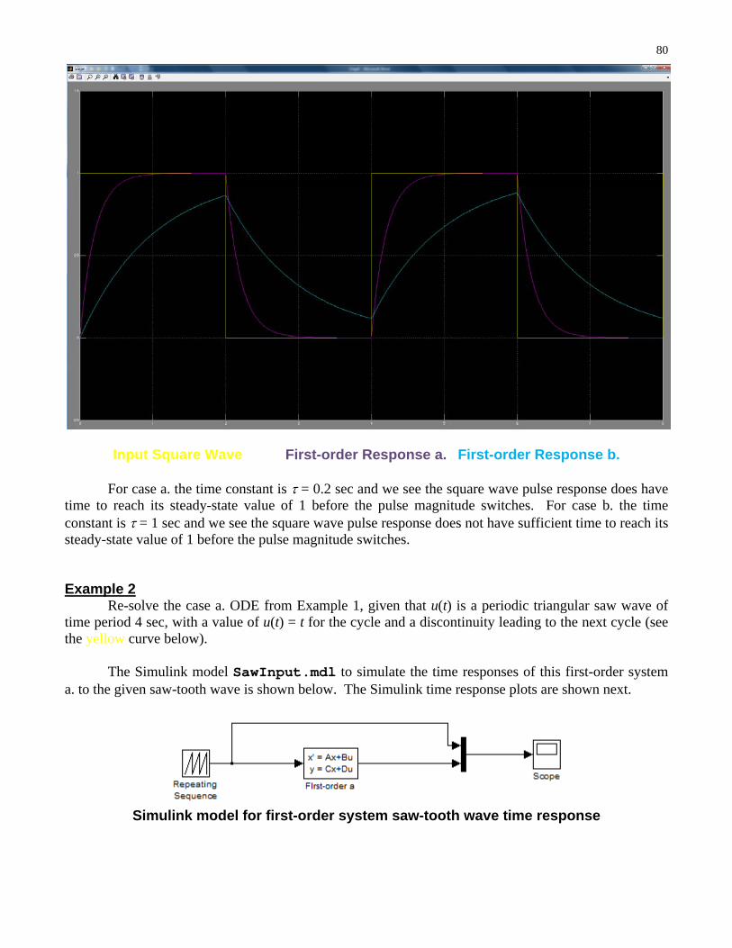
80
Input Square Wave First-order Response a. First-order Response b. For case a. the time constant is = 0.2 sec and we see the square wave pulse response does have time to reach its steady-state value of 1 before the pulse magnitude switches. For case b. the time constant is = 1 sec and we see the square wave pulse response does not have sufficient time to reach its steady-state value of 1 before the pulse magnitude switches. Example 2 Re-solve the case a. ODE from Example 1, given that u(t) is a periodic triangular saw wave of time period 4 sec, with a value of u(t) = t for the cycle and a discontinuity leading to the next cycle (see the yellow curve below).
The Simulink model SawInput.mdl to simulate the time responses of this first-order system a. to the given saw-tooth wave is shown below. The Simulink time response plots are shown next.
Simulink model for first-order system saw-tooth wave time response
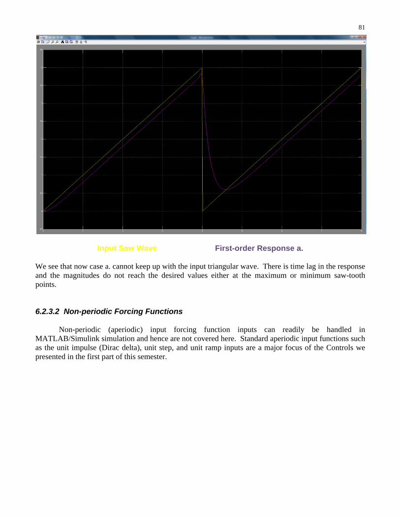
81
Input Saw Wave First-order Response a. We see that now case a. cannot keep up with the input triangular wave. There is time lag in the response and the magnitudes do not reach the desired values either at the maximum or minimum saw-tooth points. 6.2.3.2 Non-periodic Forcing Functions
Non-periodic (aperiodic) input forcing function inputs can readily be handled in MATLAB/Simulink simulation and hence are not covered here. Standard aperiodic input functions such as the unit impulse (Dirac delta), unit step, and unit ramp inputs are a major focus of the Controls we presented in the first part of this semester.

82
7. Hardware Control in the Ohio University Robotics Lab
7.1 Quanser/Simulink Controller Architecture Quanser/Simulink Controller Diagram
Quanser/Simulink Controller Hardware
External I/O Board Power Supply

83
Controlled via Quanser/Simulink
Inverted Pendulum

84
Controlled via Quanser/Simulink (continued)
8-axis NASA ARMII (Advanced Research Manipulator II)
SPAM (SPherically-Actuated platform Manipulator)

85
Controlled via Quanser/Simulink (continued)
4-dof GPS/IMU Calibration Platform
3-dof Planar 3-RPR Parallel Robot

86
Controlled via Quanser/Simulink (continued)
6-dof Spatial 6-PSU Platform
RoboCup Player Cable-Suspended Haptic Interface
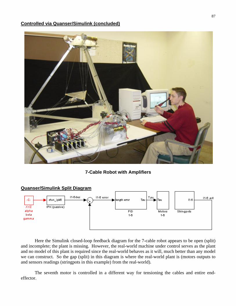
87
Controlled via Quanser/Simulink (concluded)
7-Cable Robot with Amplifiers
Quanser/Simulink Split Diagram
Here the Simulink closed-loop feedback diagram for the 7-cable robot appears to be open (split) and incomplete; the plant is missing. However, the real-world machine under control serves as the plant and no model of this plant is required since the real-world behaves as it will, much better than any model we can construct. So the gap (split) in this diagram is where the real-world plant is (motors outputs to and sensors readings (stringpots in this example) from the real-world). The seventh motor is controlled in a different way for tensioning the cables and entire end-effector.
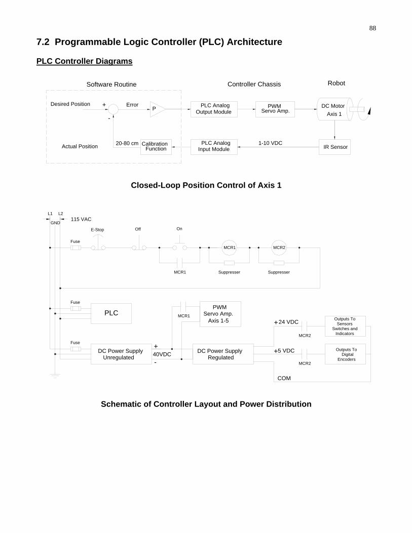
88
7.2 Programmable Logic Controller (PLC) Architecture PLC Controller Diagrams
+
-
Desired PositionP
Error
Actual Position IR SensorCalibration
Function
PLC AnalogOutput Module
1-10 VDC20-80 cm PLC AnalogInput Module
PWMServo Amp.
DC Motor
Axis 1
Software Routine Controller Chassis Robot
Closed-Loop Position Control of Axis 1
DC Power Supply
Fuse
Fuse
+DC Power Supply
Unregulated-40VDC
PLC MCR1
115 VAC
E-Stop
Fuse
GND
L1 L2
MCR1
Off On
MCR2
MCR2
+5 VDCRegulated
COM
Axis 1-5
PWMServo Amp.
24 VDC+
Outputs To
EncodersDigital
SensorsSwitches and
Indicators
Outputs To
Suppresser
MCR1
Suppresser
MCR2
Schematic of Controller Layout and Power Distribution

89
(+/- 10 VDC)
Encoder Feedback
Encoder Feedback
ServoAmp.
PWM
PWM
Amp.Servo
Amp.ServoPWM
PC Programming Terminal
5
(+/- 10 VDC)
(+/- 10 VDC)
InterfaceSerial Port
SupplyPowerPLC
(Slot) Module Type
(1) Servo Card Axis 2 & 3(2) Servo Card Axis 4 & 5
(0) Processor
(3) Analog Output(4) Analog Input(5) Digital Output(6) Digital Input
PLC 0 1 2 3 4
Ultrasonic
DC Motor
DC Motor& Encoder
& Encoder
Axis 5
Axis 2
Sensors
DC Motor
Sensor
(1-10 V)
(0-10 V)
Axis 1
IR
IndicatorsLED
SwitchesControlLimit &
Space
Expansion6 For
Power Supply
5 VDC24 VDC-
+
+ - + -
PLC Control System Hardware: Ladder Logic
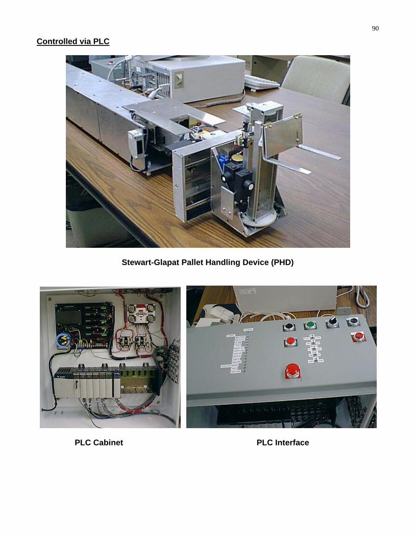
90
Controlled via PLC
Stewart-Glapat Pallet Handling Device (PHD)
PLC Cabinet PLC Interface


![FLOW-INDUCED VIBRATIONS OF A LIGHT … · FLOW-INDUCED VIBRATIONS OF A ... non-linear oscillator for self-limiting its vibration amplitude are ... [13],OngorenandRockwell[14,15],Blevins[16],MittalandTezduyar](https://static.fdocuments.us/doc/165x107/5b83b77d7f8b9a31608def45/flow-induced-vibrations-of-a-light-flow-induced-vibrations-of-a-non-linear.jpg)
