Linear Solution Techniques for Reservoir Simulation · PDF filelinear solution techniques for...

LINEAR SOLUTION TECHNIQUES FOR RESERVOIR

SIMULATION WITH FULLY COUPLED GEOMECHANICS

A REPORT

SUBMITTED TO THE DEPARTMENT OF ENERGY

RESOURCES ENGINEERING

OF STANFORD UNIVERSITY

IN PARTIAL FULFILLMENT OF THE REQUIREMENTS

FOR THE DEGREE OF

MASTER OF SCIENCE

Sergey Klevtsov

March 2017

© Copyright by Sergey Klevtsov 2017

All Rights Reserved

ii

I certify that I have read this thesis and that, in my opinion, it is fully

adequate in scope and quality as partial fulfillment of the degree of

Master of Science in Energy Resources Engineering.

(Hamdi Tchelepi) Principal Adviser

iii

Abstract

Direct modeling of geomechanics in reservoir simulation has gained a massive amount

of interest in the last decade, due both to the increase in the available computing

power and advances in numerical modeling, and to the importance of accurate repre-

sentation of mechanical effects in many unconventional reservoirs. Both fully implicit

and sequential implicit modeling approaches have been developed, with the latter

being more popular due to easier coupling of existing simulation codes. Fully im-

plicit simulation of coupled multiphase flow and poromechanics presents a challenge

to the linear solver, that must be capable of handling and efficiently solving a large

sparse linear system characterized by block structure resulting from discretizing and

linearizing the system of governing equations of mass and momentum conservation.

In this work a linear solver framework subject to the above requirements is de-

veloped, building on and extending the existing techniques, and implemented in Au-

tomatic Differentiation General Purpose Research Simulator (AD–GPRS). First, ex-

isting data structures for sparse Jacobian storage, previously specialized to flow and

transport problems with wells, are extended to handle an unlimited number of phys-

ical problems, in particular, geomechanics. Second, a generalized block–partitioned

preconditioning operator is implemented, to provide the baseline (though possibly in-

efficient) technique for handling coupled systems of equations of any kind. Finally, an

efficient preconditioning operator for multiphase flow and geomechanics is presented

based on a combination of Constrained Pressure Residual (CPR) approach and the

Fixed–stress preconditioning operator recently developed for single–phase flow. The

proposed methods are tested on several models and a clear advantage of the Fixed–

stress CPR algorithm with respect to iteration count and CPU time is shown.

iv

Acknowledgments

First of all, I am indebted to my adviser, Prof. Hamdi Tchelepi, for the opportunity

to become a part of Stanford and the reservoir simulation research group. His un-

derstanding, encouragement and guidance were invaluable during my years here, and

I’m happy to be continuing as a PhD student with his ongoing support. It is a true

honor and a privilege to be learning from Prof. Tchelepi.

I am thankful to all current and former ERE staff, faculty and researchers I’ve had

a chance to work with. Special gratitude goes to Denis Voskov for enabling my journey

to Stanford, as well as his mentorship and positive attitude. My work would not have

been possible without the help and advice from Nicola Castelletto, Timur Garipov,

Pavel Tomin and Abdulrahman Manea, to whom I am sincerely grateful. I would

also like to acknowledge Joshua White of Lawrence Livermore National Laboratory

for his collaboration.

I would like to thank all my friends, colleagues and office mates, who made this

journey a lot more fun and supported me both in and outside of study, in partic-

ular Ruslan Rin, Karine Levonyan, Christine Maier, Youssef Elkady, Jose Eduardo

Ramirez, Jamal Cherry, Vinay Tripathi and many others. I appreciate all the laughs

and meals we’ve shared over the years.

Financial support from the Department of Energy Resources Engineering and the

SUPRI-B research group and industrial affiliates consortium is kindly acknowledged.

Additional thanks are due to to TOTAL S.A. for both funding my research through

STEMS project and providing me with invaluable internship opportunities.

Finally, I am deeply grateful to my family and my wife Yulia for their unconditional

love and support.

v

Contents

Abstract iv

Acknowledgments v

1 Introduction 1

1.1 Geomechanics in Reservoir Simulation . . . . . . . . . . . . . . . . . 1

1.2 Linear Solvers . . . . . . . . . . . . . . . . . . . . . . . . . . . . . . . 3

1.3 Previous work . . . . . . . . . . . . . . . . . . . . . . . . . . . . . . . 4

1.3.1 Data Structures . . . . . . . . . . . . . . . . . . . . . . . . . . 4

1.3.2 Algorithms . . . . . . . . . . . . . . . . . . . . . . . . . . . . 5

2 Linear Solver Developments 12

2.1 Mathematical Framework for Coupled Flow and Mechanics . . . . . . 13

2.2 Data Structures Support for Mechanics . . . . . . . . . . . . . . . . . 20

2.3 Block-Partitioned Preconditioning . . . . . . . . . . . . . . . . . . . . 23

2.4 Fixed–stress CPR Preconditioning . . . . . . . . . . . . . . . . . . . . 27

3 Numerical Examples 34

3.1 Synthetic Flooding Problem . . . . . . . . . . . . . . . . . . . . . . . 35

3.2 SPE10–Based Reservoir . . . . . . . . . . . . . . . . . . . . . . . . . 41

3.2.1 Convergence . . . . . . . . . . . . . . . . . . . . . . . . . . . . 43

3.2.2 Effect of capillarity . . . . . . . . . . . . . . . . . . . . . . . . 44

vi

4 Concluding Remarks 49

4.1 Conclusions . . . . . . . . . . . . . . . . . . . . . . . . . . . . . . . . 49

4.2 Future Work . . . . . . . . . . . . . . . . . . . . . . . . . . . . . . . . 50

Bibliography 52

vii

List of Tables

3.1 Synthetic flooding test, model parameters. . . . . . . . . . . . . . . . 36

3.2 Synthetic flooding test, grid dimensions and problem size. . . . . . . . 37

3.3 Synthetic flooding test: average number of GMRES iterations per New-

ton step. . . . . . . . . . . . . . . . . . . . . . . . . . . . . . . . . . . 38

3.4 Synthetic flooding test, linear solver time in seconds. . . . . . . . . . 40

3.5 SPE10–based test, grid dimensions and problem size. . . . . . . . . . 42

3.6 SPE10-based reservoir: model parameters. . . . . . . . . . . . . . . . 43

viii

List of Figures

1.1 Multi Level Sparse Block matrix format schematics. . . . . . . . . . . 6

1.2 Illustration of CPR reduction process. . . . . . . . . . . . . . . . . . . 9

2.1 Example of Jacobian structure with geomechanics. . . . . . . . . . . . 20

2.2 Extended Multi Level Sparse Block matrix format grid layout. . . . . 21

2.3 Example of a preconditioning tree structure. . . . . . . . . . . . . . . 26

3.1 Synthetic flooding test, model setup. . . . . . . . . . . . . . . . . . . 36

3.2 Synthetic flooding test, convergence results. . . . . . . . . . . . . . . 39

3.3 Synthetic flooding test, scaling. . . . . . . . . . . . . . . . . . . . . . 41

3.4 Permeability fields for SPE10-based test case: kx, ky (top row), kz

(bottom row). . . . . . . . . . . . . . . . . . . . . . . . . . . . . . . . 42

3.5 SPE10–based test, convergence on fine and upscaled grids. . . . . . . 44

3.6 SPE10–based test, influence of capillarity on convergence. . . . . . . . 46

3.7 SPE10–based test without mechanics, influence of capillarity on con-

vergence. . . . . . . . . . . . . . . . . . . . . . . . . . . . . . . . . . . 47

3.8 SPE10–based test, ratio of convergence of CPR–FS vs. CPR scheme. 48

ix

Chapter 1

Introduction

1.1 Geomechanics in Reservoir Simulation

Conventional reservoir simulation deals with solving partial differential equations gov-

erning multiphase multicomponent flow in a porous medium over the domain of in-

terest. As time goes on and simulation techniques get more mature, more and more

complex models and interacting physical phenomena are being introduced in simula-

tors, which turns it into a coupled multi-physics problem. Examples include extending

simulator capabilities to deal with heat flow, chemical reactions and geomechanics.

The latter is of particular interest, because accurate modeling of subsurface mechan-

ical effects plays a critical role in predicting reservoir performance and behavior and

assessing the safety of oil field and CO2 sequestration operations. Many physical

phenomena, such as compaction, subsidence, wellbore failure and change in matrix

and fracture permeability can be modeled and explained with geomechanics.

Traditionally, reservoir simulators have simplified the mechanical rock response by

reducing it to a single uniaxial compressibility coefficient (usually assumed constant).

However, in particular due to the increased interest in unconventional resources, such

as shales, multiple efforts have been made to integrate proper geomechanical modeling

1

CHAPTER 1. INTRODUCTION 2

in reservoir simulators, efforts required because of the tight coupling and complex

dynamics taking place between the flow and mechanical problems. A number of

solution strategies have been proposed, including [7]:

• Loosely coupled, where the coupling between the two problems is resolved only

at certain time intervals. This approach is the least computationally expensive

as it involves far fewer mechanics solves, but its accuracy cannot be reliably

estimated a priori.

• Iteratively coupled, where one of the two problems (either flow and transport or

mechanics) is solved first to obtain an intermediate solution estimate, and then

the other problem is solved using this solution; the process is iterated until the

desired convergence tolerance is achieved. Like the loosely coupled approach,

this approach allows to use separate simulation codes for flow and mechanics,

but this scheme is accurate, resulting in the same solution as the fully coupled

one. Based on the manner in which the variables of each problem are fixed, a

number of schemes have been devised, some of which are unconditionally stable.

Still, a number of sequential iterations (between flow and mechanical parts) may

be required.

• Fully coupled, where the equations governing flow, transport and geomechan-

ics are discretized and solved simultaneously at every time step. This scheme

is always accurate and unconditionally stable. However, it requires investing

additional effort in developing a unified simulator capable of handling multi-

ple physical problems, both on the nonlinear (discretization schemes, nonlinear

loop and Newton-Raphson linearization) and linear (solving a large fully cou-

pled linear system) levels.

For the reasons mentioned above, most activity in this area has been directed

towards the iterative coupling schemes ([11]), and relatively few efforts have been


invested in fully coupled simulators. Difficulties associated with generating fully cou-

pled Jacobian matrices can be overcome with automatic differentiation (AD) tech-

niques. Recently, an AD library, ADETL [26], has been developed by R. Younis

targeting reservoir simulation applications. It became the basis for AD-GPRS [23],

Stanford’s in-house simulator, with capabilities for solving flow, transport, thermal

and geomechanical problems using different coupling strategies (both sequential and

fully implicit schemes).

Fully implicit simulation poses additional challenges for the linear solver, which

must be capable to efficiently handle large linear systems with multiple sets of un-

knowns and a distinct block structure in the matrix arising from discretizing multiple

types of governing equations. Therefore moving to fully coupled multiphysics simu-

lation encourages development of specialized linear solution techniques.

1.2 Linear Solvers

The linear solver is one of the most crucial and performance-critical components of

a reservoir simulator. In a typical simulation it can take anywhere between 40% and

80% of the total runtime. Due to the size of problems to be solved, use of direct

solvers is computationally infeasible, and iterative solvers are preferred. Typically

used algorithms include Krylov subspace methods, such as Orthomin, GMRES and

BiCGStab [18], which are known to be the most efficient. However, they rely on

preconditioning of the linear system to accelerate convergence, that is, improving

the condition number of the matrix by pre– or post–multiplying the matrix by a

preconditioning operator P :

P−1Ax = P−1b AP−1Px = b


Note that in the context of iterative linear solvers, the only operation required is

application of P−1 to vectors. A preconditioner can therefore be viewed as a black

box operator, acting on a vector v and producing another vector w = P−1v, which

is the approximate solution of Aw = v, since the operator is chosen such that P−1

resembles A−1 in some sense, while being much cheaper to construct than the actual

inverse. Any solver, including a Jacobi-type smoother, a nested Krylov iteration, a

multigrid method, an incomplete factorization, or a block-partitioned scheme, can be

used as a preconditioner.

1.3 Previous work

The linear solver framework in AD-GPRS is largely based on the work of Y. Jiang

[10], who developed both the data structures and the solver code, which has been

later extended by Y. Zhou [28]. Here the main features of the linear solver framework

are described.

1.3.1 Data Structures

Efficient sparse data structures are required to store and manipulate the linear sys-

tem during the solution. The Multi Level Sparse Block (MLSB) data structure is

a hierarchical matrix storage format that highlights the separation of the original

system into individual blocks (or subproblems) and facilitates the development of

specialized preconditioning strategy. On the top level, and MLSB matrix is just a

storage container for nested reservoir (JRR) and facilities (JFF matrices, together

with coupling blocks (JRF and JFR). In this notation the first subscript index is used

to denote the type of equation (reservoir of facilities) and the second index is the

type of variables the derivative is taken with respect to. Individual submatrices are

allowed to have any internal representation. For instance, the reservoir matrix JRR


is stored in a customized block CSR (Compressed Sparse Row) format that empha-

sizes the block ordering of independent simulation variables and is particularly well

suited for Adaptive Implicit Method (AIM) Jacobians. The facilities matrix JFF in

turn is another storage container for individual facility submatrices, whose storage

format depends on the facility models used and can include more nested submatrix

levels. The reservoir-facility coupling blocks JRF and JFR are also containers for

individual facility coupling blocks, which are typically stored in coordinate (COO)

format. The key feature of this approach is that all matrices and matrix blocks share

a common interface, that includes operations like extraction from AD residuals, var-

ious forms of algebraic reduction (for example, from full system to primary and from

primary to implicit system), matrix-vector operations required by iterative solvers

and output in human– and machine–readable formats. These operations are defined

recursively, with upper–level matrices calling submatrices to execute operations. At

the same time, implementation details are completely hidden from the upper level

matrices. Thus the MLSB format was designed to provide convenient abstraction

and organization of systems with several coupled physical models. Existing imple-

mentation, however, has been limited to reservoir-well systems only, despite initially

flexible high-level design. The fact that each physical model is stored in a separate

container allows for easy extraction of individual blocks and implementing efficient

specialized linear and nonlinear solution strategies. The high-level representation of

the format is shown in Figure 1.1.

1.3.2 Algorithms

The second important part of the framework is a collection of solution algorithms.

AD-GPRS linear solver framework provides interfaces to a number of external solver

libraries (such as SuperLU [8, 15], PARDISO [20] and SAMG [21]), as well as it’s own

set of iterative solvers. The latter is of primary interest, since it allows to perform


JRR

JFF

JRF

JFR JWW1JWW

2JWW

3

JRW1JRW

2JRW

3

JWR1

JWR2

JWR3

Figure 1.1: Multi Level Sparse Block matrix format [10] schematics.

research on efficient specialized solution strategies; however, external libraries are

often used as building blocks for more complex solution algorithms. Despite the fact

that matrix size is reduced after full to primary and primary to implicit linear system

reductions, it still remains significant (often on the order of 106 and larger), especially

in fully implicit simulations.

Krylov subspace iterative solvers are perhaps the most robust and widely used

family of solvers. A nice common feature of them is independence of the details of

matrix structure, that is, only the typical BLAS operations (matrix–vector product,

axpy, dot products) need to be defined. This makes Krylov solvers perfectly suited

to working with MLSB hierarchical matrices. In particular, GMRES [19] is known

for its superior performance when used in conjunction with a good preconditioner.

It guarantees monotone convergence of residual norm ||b − Ax||2 to zero within N

(size of the system) iterations, however in practice the actual number of iterations


required to converge to the desired tolerance is much smaller than N . In addition,

the algorithm is typically restarted every m iterations (with m anywhere between 20

and 100) in order to keep memory requirements and numerical round-off error under

control.

CPR Preconditioning

Convergence properties of Krylov subspace methods depend strongly on the avail-

ability of a high quality preconditioner. It is well-known that some generic families

of preconditioners, such as, for instance, the Incomplete LU factorizations (ILU) [18],

can be easily applied to any type of matrix, but their effectiveness varies from problem

to problem and in general is suboptimal. On the other hand, specialized precondition-

ing strategies for reservoir simulation equations have been developed, among them

the Constrained Pressure Residual [24] is perhaps the most efficient and well known.

Here we briefly describe the idea and existing implementation of CPR.

Reservoir simulation equations are those of mass conservation (secondary ther-

modynamic and linear constraint equations are local and are taken care of during

the first step of the algebraic reduction process mentioned previously). They implic-

itly include a near–elliptic diffusion part (through the pressure primary unknown)

and near–hyperbolic advection part (through saturation, phase composition or other

choices of primary unknowns), and as such, exhibit a mixed nature. The CPR pre-

conditioning is a two-stage strategy based on the idea of isolating the near-elliptic

part by constructing a pressure equation algebraically on the linear level and solving

for an approximate pressure solution using an efficient elliptic solver (such as a few

steps of a multigrid or multiscale method), which resolves global long-range error

modes in the residual. The remaining degrees of freedom are treated in the second

stage by a local smoother, such as ILU(k) (or its block counterpart, BILU(k)), which

removes the high frequency local errors. The overall preconditioning scheme Pcpr can


be represented as follows:

P−1cpr = P−1

sm(I − JP−1p ) + P−1

p (1.1)

where Pp is the first–stage pressure preconditioner, Psm is the second–stage smoother,

J is the Jacobian matrix and I is an identity operator.

A detailed description of CPR implementation can be found in [28]. Here a high-

level view of the preconditioning operator is presented. We begin with a fully implicit

linear system that has a distinct block structure:

Jδx = r or

Jss Jsp

Jps Jpp

δxsδxp

=

rs

rp

(1.2)

Here we use subscript p to denote pressure and s for all other implicit variables.

Since there is no dedicated pressure equation in a FIM system, we choose the first

equation in each block as the pressure equation (corresponding to the pressure un-

known, which is also first in each block). Note that in the actual implementation

the degrees of freedom are not split into global blocks, but rather are interleaved and

arranged on a block–by–block basis. Here, for the simplicity of algebraic formulation

of the method, we rearrange them equivalently to separate the pressure block. An

example structure of such Jacobian on a 3D structured grid is shown in Figure 1.2a.

All four blocks have the same block nonzero sparsity structure defined by the grid

connectivity, with only the size of the blocks being different.

Construction of the pressure system is carried out through a process called True-

IMPES reduction, which begins by applying simplifying assumptions to the Jaco-

bian, namely, explicit treatment of all non–pressure unknowns in flux terms. This is

achieved purely on the linear level by applying a column summation operator C, which

adds off-diagonal elements in each block column into the corresponding diagonal block


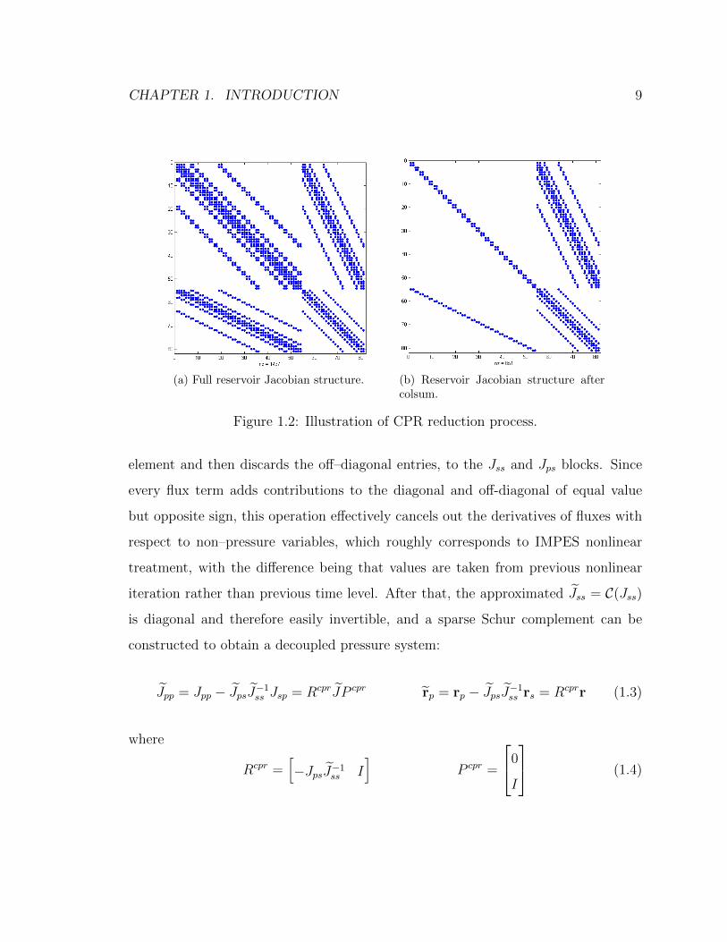
(a) Full reservoir Jacobian structure. (b) Reservoir Jacobian structure aftercolsum.

Figure 1.2: Illustration of CPR reduction process.

element and then discards the off–diagonal entries, to the Jss and Jps blocks. Since

every flux term adds contributions to the diagonal and off-diagonal of equal value

but opposite sign, this operation effectively cancels out the derivatives of fluxes with

respect to non–pressure variables, which roughly corresponds to IMPES nonlinear

treatment, with the difference being that values are taken from previous nonlinear

iteration rather than previous time level. After that, the approximated Jss = C(Jss)

is diagonal and therefore easily invertible, and a sparse Schur complement can be

constructed to obtain a decoupled pressure system:

Jpp = Jpp − JpsJ−1ss Jsp = RcprJP cpr rp = rp − JpsJ−1

ss rs = Rcprr (1.3)

where

Rcpr =[−JpsJ−1

ss I]

P cpr =

0

I

(1.4)


The resulting pressure matrix structure is that of the Jpp block; the Schur comple-

ment changes its entries but does not affect sparsity pattern. After the approximate

pressure solution is obtained, it is prolongated to the full solution vector and the

right–hand side is updated accordingly:

r2 = r− Jδx1 = r− JP−1p r = [I − JP−1

p ]r (1.5)

Finally, applying a second-stage smoother to the full system with an adjusted

residual yields an update to both pressure and non–pressure unknowns, which is

combined with the first stage pressure solution for the final result:

δx = δx1 + δx2 = P−1p r + P−1

smr2 = P−1p r + P−1

sm[I − JP−1p ]r =

= [P−1p + P−1

sm[I − JP−1p ]]r = Pcprr

(1.6)

Wells are naturally incorporated within the CPR strategy. Standard well models

have only a single unknown, the bottom hole pressure pw, which is simply kept in

the first-stage pressure system and solved for together with reservoir block pressures.

Multisegment wells are first reduced to a single pressure unknown and then treated

similarly [27], [28]. Note that construction of the restriction and prolongation opera-

tors, as well as setup of the pressure solver and smoother (all expensive operations)

in CPR need to be performed only once per nonlinear iteration (when the matrix

changes), while application these operators (relatively cheap) occurs on every lin-

ear iteration (since they need to be applied to each newly constructed vector of the

Krylov subspace). Overall, CPR with highly optimized kernels has been shown to be

a very robust and powerful preconditioner for reservoir simulation with standard and

multisegment wells ([2], [10], [28], [3]).


Concluding Remarks

CPR is an example of a multi-stage preconditioning scheme. In general form, such

schemes can be expressed as follows [3]:

P−1 =n∑i=1

P−1i

i−1∏j=1

[I − JP−1

j

](1.7)

where Pi is the preconditioner used at i–th stage, and for i = 1 the product term is

defined to be equal to identity. This notation describes the consecutive application

of stages, with and adjustment of the residual between stages. Note that each stage

Pi may have a reduction and prolongation operators implicitly built-in.

Multistage/block–partitioned preconditioning is a powerful idea that can be ex-

ploited to implement strategies for any number of coupled problems, including but

not limited to flow, mass transport, geomechanics and heat flow and transport. In

the next chapter we develop the idea of a multistage preconditioner for coupled mul-

tiphase flow and transport with geomechanics.

Chapter 2

Linear Solver Developments

Advancements in geomechanical modeling and ongoing incorporation of mechanical

models in reservoir simulators necessitates the development of efficient linear solution

and preconditioning techniques for systems arising from fully implicit discretization.

The size of these systems is much larger than those in conventional reservoir simula-

tion. For example, on a structured 3D grid with a large number of grid blocks the

total number of nodes in the limit is approximately equal to the number of blocks.

With 3 additional mechanical unknowns per node (components of displacement vector

u, the size of the systems is twice as large as a regular simulation with 3 unknowns

per cell (e.g. a Black–Oil model). In addition, the mechanical domain is typically

taken much larger than that of fluid flow, in order to specify boundary conditions

properly for the domain of interest, which could result in an even larger system. All

of this indicates an efficient and scalable preconditioner is required to handle such

systems.

In this chapter first the mathematical and numerical framework used for mod-

eling is described to provide a foundation for discussion of linear systems arising

during simulation. Then the necessary extensions to the linear solver framework of

AD-GPRS are discussed, including both data structures and algorithms, and a new

12

CHAPTER 2. LINEAR SOLVER DEVELOPMENTS 13

efficient preconditioning scheme is detailed.

2.1 Mathematical Framework for Coupled Flow and

Mechanics

The principal equations governing multiphase multicomponent flow and mechan-

ics in porous medium are those of mass and momentum conservation. The multi-

phase poromechanics problem is formulated after [6] in terms of displacement and

fluid pressure unknowns and natural variables [2] (saturation/phase composition) for

transport. We are considering an arbitrary porous domain Ω ∈ R3 with bound-

ary Γ with a normal vector n that is partitioned into non–overlapping regions as

Γ = Γu ∪ Γσσσ = Γp ∪ Γq for the purpose of specifying boundary conditions.

Assuming isothermal conditions and infinitesimal displacements, and neglecting

capillary pressure effects (thus, pp = p for each phase p) the strong form of the

initial/boundary value problem can be stated as: find u, p, Sp and xcp, p = 1..Np, c =

1..Nc, over the domain Ω and time interval T = [0, T ] such that

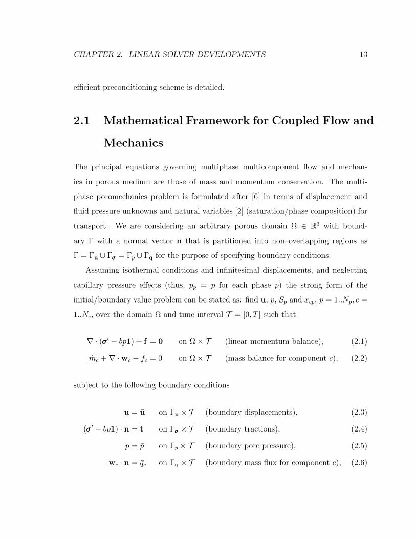
∇ · (σσσ′ − bp1) + f = 0 on Ω× T (linear momentum balance), (2.1)

mc +∇ ·wc − fc = 0 on Ω× T (mass balance for component c), (2.2)

subject to the following boundary conditions

u = u on Γu × T (boundary displacements), (2.3)

(σσσ′ − bp1) · n = t on Γσσσ × T (boundary tractions), (2.4)

p = p on Γp × T (boundary pore pressure), (2.5)

−wc · n = qc on Γq × T (boundary mass flux for component c), (2.6)


and initial conditions for ξ ∈ Ω

u(ξ, 0) = u0(ξ) (initial displacements), (2.7)

p(ξ, 0) = p0(ξ) (initial pore pressure), (2.8)

Sp(ξ, 0) = S0p(ξ) (initial saturation for fluid phase p), (2.9)

xcp(ξ, 0) = x0cp(ξ) (initial mole fraction of component c in phase p). (2.10)

Here, σσσ′ is effective stress tensor; b is the Biot coefficient; 111 is the second-order unit ten-

sor; f is the body force vector, which is assumed constant here; mc =

(Np∑p=1

φρpSpxcp

),

wc and fc denote mass, mass flux and source/sink term for component c = 1..Nc,

with φ and ρp porosity and fluid phase density, respectively; ξ is the position vector in

R3; ∇· and ∇ are the divergence and gradient operator, respectively. The superposed

dot, (), denotes a derivative with respect to time.

The formulation is completed by the addition of appropriate constitutive relation-

ships. In particular, a fourth-order tensor of drained tangential moduli, Cdr, relates

σσσ′ to u via the the linearized second-order strain tensor, εεε. In general incremental

form such relationships reads:

∆σσσ′ = Cdr : ∆εεε, (2.11)

εεε = ∇su =1

2

(∇u +∇Tu

), (2.12)

where ∇s is the symmetric gradient operator, and (:) denotes a tensor product con-

tracted on two indices. Following [6], porosity is modeled as:

∆φ = b∆εv +(b− φ0)

Ks

∆p, (2.13)

where εv = trace(εεε) is the volumetric strain, and Ks = K/(1 − b) is the solid phase


bulk modulus, with K the skeleton bulk modulus. Note that Biot’s coefficient is

restricted to the interval φ < b ≤ 1, with b = 1 representative of the incompressible

solid phase limit case [9]. Mass flux for each component is given by wc =Np∑p=1

ρpvpxcp,

which makes use of the classic multiphase flow generalization of Darcy’s law [1]:

vp = −krpµpkkk · (∇p− ρpg) , (2.14)

where kkk is the absolute permeability tensor; µp and krp are the viscosity and relative

permeability factor for fluid phase p, respectively; and g is the gravity vector.

The source/sink terms fc =Np∑p=1

qpρpxcp in Equation (2.2) represent the effects of

well production/injection and are typically line sources. These are governed by a

suitable well model with certain assumptions—typically radial flow in the vicinity of

the wellbore, that relates well control parameters, such as bottom hole pressure, to

phase volumetric flow rates qp through the wellbore.

The system of equations is closed by adding local thermodynamic equilibrium

constraints in the form of fugacity equality relations:

fcp1(P,xp1) = fcp2(P,xp2), ∀p1, p2 = 1..Np, ∀c = 1..Nc, (2.15)

and linear saturation/composition constraints

Np∑p=1

Sp = 1, (2.16)

Nc∑c=1

xcp = 1, ∀p = 1..Np. (2.17)

The initial/boundary value problem (2.1)–(2.10) is discretized in space by a mixed


finite–element (FE)/finite–volume (FV) approach. A single conforming computa-

tional grid that partitions Ω in nelem non–overlapping elements Ωe (control volumes

in the finite-volume terminology) is used. The balance of linear momentum is solved

based on the following variational formulation:

Rmom. = −∫

Ω

∇sηηη : σσσ′ dV +

∫Ω

bp∇ · ηηη dV +

∫Ω

ηηη · f dV +

∫Γσσσ

ηηη · tσ dA = 0 ∀ηηη,

(2.18)

with η appropriate weighting functions. In particular, η varies over the spaces

(H1(Ω))3, and satisfies homogeneous boundary conditions on the essential bound-

aries Γu. Here, H1 is a Sobolev space of degree one. The derivation of the discrete

form of the mass balance equations consists of writing Equation (2.2) for a generic

Ωe in integral form. Making use of divergence theorem leads to the following set of

balance equations for each fluid component c = 1..Nc:

Rmassc,e =

∫Ωe

mc dV +∑j∈Je

wc,ej −∫

Ωe

fc dV = 0 e = 1, . . . , nelem (2.19)

where Je denotes the set of indices j of elements Ωj sharing a face with Ωe, and wc,ej

are the inter-element integral fluxes

wc,ej =

∫Γej

wc · nej dA, (2.20)

with nej the unit normal vector to Γej oriented from Ωe to Ωj.

The final discrete form is obtained based on a suitable time and space discretiza-

tion of the set of residual equations (2.18)–(2.19). Time integration relies on the

first–order accurate, unconditionally stable backward Euler scheme. The displace-

ment field, u, is approximated with trilinear (Q1) finite elements while a piecewise


constant interpolation (P0) is used for both the pressure field p, and the fluid phase sat-

uration, Sp, and composition, xcp, fields. As far as the approximation of fluxes (2.20)

is concerned, either a two–point flux (TPFA) or a multi–point flux (MPFA) approxi-

mation can be used, depending on the grid. Let xn = [Sn,xn,un,pn]T be the discrete

solution at time tn. The solution xn+1 at time tn+1 = (tn+ ∆t) is obtained by solving

the following discrete system of equations

r(xn+1,xn

)=

rmass

rmom.

= 0, (2.21)

with the residual vector r being assembled as sum of element contributions. Specif-

ically, the element–wise contributions to the discrete residual vector for the generic

Ωe read:

[rmom.]i =−∫

Ωe

∇sηηηi : σσσ′,n+1 dV +

∫Ωe

bpn+1∇ · ηηηi dV +

∫Ωe

ηηηi · fn+1 dV

+

∫Γσσσ,e

ηηηi · tn+1dV, i = 1, 2, . . . , nu (2.22)

[rmassc ]e =

1

∆t

∫Ωe

(mn+1c −mn

c

)dV −

∑j∈Je

Tejλn+1p,ej

(Φn+1p,j − Φn+1

p,e

)−∫

Ωe

fn+1c dV

(2.23)

where vector functions ηi are the finite element bases for the displacement, with nu

the number of displacement degrees of freedom; Tej is the geometric transmissibility of

interface Γej; Φp,k = (pp,k − ρp,k |g| dk) is the p-th fluid phase flow potential evaluated

at the k–th cell centroid depth, dk; and λp,ej is the p–th fluid phase mobility computed


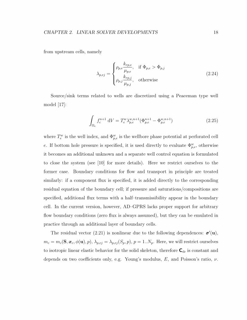
from upstream cells, namely

λp,ej =

ρp,e

krp,eµp,e

, if Φp,e > Φp,j

ρp,jkrp,jµp,j

, otherwise

(2.24)

Source/sink terms related to wells are discretized using a Peaceman type well

model [17]:

∫Ωe

fn+1c dV = Twe λ

w,n+1p,e (Φn+1

p,e − Φw,n+1p,e ) (2.25)

where Twe is the well index, and Φwp,e is the wellbore phase potential at perforated cell

e. If bottom hole pressure is specified, it is used directly to evaluate Φwp,e, otherwise

it becomes an additional unknown and a separate well control equation is formulated

to close the system (see [10] for more details). Here we restrict ourselves to the

former case. Boundary conditions for flow and transport in principle are treated

similarly: if a component flux is specified, it is added directly to the corresponding

residual equation of the boundary cell; if pressure and saturations/compositions are

specified, additional flux terms with a half–transmissibility appear in the boundary

cell. In the current version, however, AD–GPRS lacks proper support for arbitrary

flow boundary conditions (zero flux is always assumed), but they can be emulated in

practice through an additional layer of boundary cells.

The residual vector (2.21) is nonlinear due to the following dependences: σσσ′(u),

mc = mc(S,xc, φ(u), p), λp,ej = λp,ej(Sp, p), p = 1..Np. Here, we will restrict ourselves

to isotropic linear elastic behavior for the solid skeleton, therefore Cdr is constant and

depends on two coefficients only, e.g. Young’s modulus, E, and Poisson’s ratio, ν.


Newton’s method is used to drive r to zero:

J(xn+1,k

)δx = −r

(xn+1,k,xn

), (2.26)

xn+1,k+1 = xn+1,k + δx, (2.27)

with J the Jacobian matrix evaluated at Newton step k. In the rest of this work,

for the sake of convenience, we label both saturation and composition unknowns

with a lowercase s; additionally, even though all component mass balance equations

are similar, we arbitrarily choose the first one in each cell and label it as ’pressure’

(p) equation, to correspond to the pressure unknown, which is always first in each

cell. Finally, although equations are written cell–by–cell (or node–by–node), we can

rearrange all equations and unknowns based on the unknown type (saturation/com-

position, displacement or pressure), for convenience of algebraic notation. With this,

the Jacobian matrix of the system can be written as:

J(xn+1,k

)=

∂rmass2..Nc

∂s

(xn+1,k

) ∂rmass2..Nc

∂u

(xn+1,k

) ∂rmass2..Nc

∂p

(xn+1,k

)∂rmom.

∂s

(xn+1,k

) ∂rmom.

∂u

(xn+1,k

) ∂rmom.

∂p

(xn+1,k

)∂rmass

1

∂S

(xn+1,k

) ∂rmass1

∂u

(xn+1,k

) ∂rmass1

∂p

(xn+1,k

)

=

Jss Jsu Jsp

Jus Juu Jup

Jps Jpu Jpp

(2.28)

An example structure of such Jacobian matrix is shown in Figure 2.1, except that

flow/transport unknowns are not rearranged into separate blocks. Note that all local

equations, including fugacity and linear constraints (2.15)–(2.17), are reduced during

linearization process (either at AD level or algebraically) and do not appear in the final

Jacobian. Additionally, as noted before, for simplicity we ignore well equations and

unknowns in this discussions, restricting ourselves to bottom hole pressure controls,

but they are naturally handled both by data structures and algorithms ([10, 28]).


0 200 400 600 800 1000 1200 1400

nz = 50590

0

200

400

600

800

1000

1200

1400

Figure 2.1: Example of Jacobian structure with reservoir, wells and geomechanics.

2.2 Data Structures Support for Mechanics

In order to store and manipulate systems with flow and geomechanical parts, the

data structures used on the linear level must be made mechanics–aware. Luckily, the

design of MLSB matrix format used in AD-GPRS is flexible enough to allow for such

an extension. Previously, the system matrix has been implemented as a container

with a fixed number of inner blocks (reservoir, facilities and couplings), templated on

the type of those blocks so that implementation could be switched easily. Foreseeing

future extensions to heat flow and other problems, instead of adding another inner


JRR

JFF

JGG

JXX

JRF

JFR

JRG

JGR

JXR

JRX

JGX

JXGJXF

JFX

JRR*

JFF*

JRF*

JFR*

extractBlocks

([RESERVOR_BLOCK,

FACILITIES_BLOCK]

Figure 2.2: Extended Multi Level Sparse Block matrix format grid layout and sub-matrix extraction. X represents an arbitrary coupled subproblem.

block (together with relevant coupling blocks) into the fixed-size container, we reim-

plemented it as a dynamic container called BlockMatrixWrapper capable of holding

a potentially unlimited (subject to memory considerations) number of blocks (see

Figure 2.2 for a high-level representation of the extended MLSB matrix). Thus, a

static polymorphism based implementation had to be switched with a dynamic one

(with dynamic overhead being minimal, since these are high-level objects). It should

be noted that not all coupling blocks may be present in the system, for example there

may be no direct coupling between geomechanical problem and facilities (wells). The

container, visually represented as a two-dimensional grid of submatrices, must there-

fore allow some of them to be missing (null).

In order to properly adhere to the requirements of MLSB matrix interface, the


necessary operations have been implemented in BlockMatrixWrapper, such as, ex-

traction from AD residual, calculation of size, sparse matrix–vector product, alge-

braic reductions, output and other. Most of them delegate work to submatrices and

then accumulate the results, if necessary. Care has to be taken to call submatrices in

appropriate order, for instance, the coupling blocks depend on their respective diag-

onal master blocks for size calculations. Moreover, while most operations are easily

parallelizable across the submatrices (using OpenMP shared–memory parallelization

directives), one must watch out for potential data races and dependencies, and load

balancing between threads is likely to be far from perfect, since the amount of work

to be done per submatrix varies significantly.

An additional operation has been added to the MLSB interface and implemented

for all matrix types — extraction into CSR format, which is required for better

interoperability with external solver libraries. The top level block matrix wrapper

performs this by extracting each submatrix into CSR and then recursively merging

them, first within each block row (horizontally) and then merging together block rows

(vertically). It should be noted that, due to row orientation of CSR, while a vertical

merge is relatively cheap (just a concatenation of the three storage arrays and trivial

update of row pointers), a horizontal merge is quite a bit more expensive, requiring

interleaving data from multiple matrices, and a more optimal implementation of this

process may be sought.

In addition to standard MLSB interface, the block matrix wrapper features addi-

tional methods for access to individual blocks, as well as extraction groups of blocks

into a new block matrix wrapper object. In order to identify blocks by their con-

tents rather than their position in the grid (which can change if the clients of linear

solver framework decide to change the relative order of subproblems in AD residual),

each subproblem is assigned a meaningful tag during matrix initialization, such as


RESERVOIR BLOCK, GEOMECHANICS BLOCK and so on. The user then pro-

vides a tag or set of tags for blocks they would like to access or extract. During

extraction, a new block wrapper is created that contains pointers to original matrix

blocks, but the blocks themselves are not copied; the new object is thus a shallow copy

and operates in reference mode. If desired, a deep copy may be created as well, but

this is usually not required, since all algorithm implementations leave the matrices

untouched and create their own copies of data whenever an in–place modification is

required. The shallow copy matrix wrapper represents a convenient object for per-

forming matrix-vector operations with and forms the basis for our implementation of

block-partitioned preconditioning.

2.3 Block-Partitioned Preconditioning

The Constrained Pressure Residual preconditioner considered in section 1.3.2 is a

highly specialized preconditioner tailored to a particular set of equations. However,

the basic idea of multistage preconditioning utilized in CPR can in principle be gen-

eralized to any given problem. Stages can be used to separate (decouple on the linear

level) and tackle different physical phenomena or different spatial subdomains. In

particular, in domain decomposition methods a well-known family of preconditioners

are additive and multiplicative Schwartz, which have a direct correspondence to block

versions of Jacobi and Gauss–Seidel iterations [18]. Similar ideas can be applied to

the case where virtual ’subdomains’ correspond to different mathematical equations.

Based on these observations, a generic sequential preconditioning scheme for cou-

pled problems was implemented in AD-GPRS as a baseline approach, against which

other, more advanced schemes can be compared. We refer to it as block–partitioned

preconditioning.

The design objective was to create a flexible implementation, that can be easily


configured for any set of coupled equations at hand, provided that solvers for individ-

ual equations are available. To that end, the implementation is based on a recursive

tree structure (see Figure 2.3). Each leaf node corresponds to a particular subprob-

lem associated with a solver, and each internal node represents a set of subproblems

(its child nodes) that are solved together to desired criteria (residual norm or a given

number of iterations) via an iterative scheme — either Jacobi–like or Gauss–Seidel–

like. The difference between the two block-partitioned schemes is the same as in

their pointwise counterparts: in Jacobi all blocks are solved independently and then

the right-hand side is updated with solutions before proceeding to the next iteration;

while in Gauss–Seidel the right–hand side is updated after each block solve. Due to

less lag in the right–hand side, Gauss–Seidel typically converges faster, at the cost of

not being able to parallelize simultaneous solution of multiple bocks. The latter is

much less of an drawback in large models, where each block is already large enough

so that parallelization of individual block solvers yields significant benefits.

Listing 2.1 shows a simplified example declaration of a preconditioning tree node.

In addition to control parameters such as iteration type, tolerance and number of

iterations, each nodes also contains a list of associated block tags (leaf nodes have

only one, while intermediate have multiple), that are used to extract the submatrix

from the master block matrix, and a shallow copy block matrix with block pointers

(described in Section 2.2). Intermediate nodes also keep a set of right–hand side and

solution vectors for each block, as those will change during the iteration, and leaf

nodes maintain a pointer to the solver (preconditioner) to be used for current block.

During both setup and solve phases, block–partitioned preconditioner performs a

depth–first traverse of the tree. At setup, the blocks are extracted from the given

matrix (again, this operation is cheap as it is nothing more than creating pointers to

blocks) and leaf preconditioner setup is performed. During solve, child branches may

be traversed multiple times until the intermediate node convergence criteria are met.


Listing 2.1: Example of a preconditioning tree node declaration.

struct PrecondNode

enum IterType GAUSSSEIDEL = 0, JACOBI = 1 ;

bool isLeaf;

BlockMatrixWrapper* matrix;

std::vector <BlockType > block_types;

// for intermediate nodes

std::vector <PrecondNode*> child_nodes;

std::vector <Vector > rhs_ectors;

std::vector <Vector > sol_vectors;

IterType iter_type;

int num_iter;

double tolerance;

// for leaf nodes

SolverBase* precond;

;


Figure 2.3: Example of a preconditioning tree structure. Top level is one Gauss-Seideliteration between reservoir flow with wells and geomechanics, which amounts to justsolving them in turn. Middle level includes a Jacobi iteration between reservoir andwells until a tolerance of ε = 10−3, which means solving them independently, updatingthe right–hand side and iterating until convergence.

Thus, a solution strategy is defined recursively and may have multiple levels. For

instance, we may wish to solve reservoir flow and facilities to a certain tolerance, and

then combine with geomechanical solution in an outer iteration. As more and more

subproblems are being added, more complicated strategies with many levels may be

devised. Presently, however, the only problems considered are reservoir flow and

transport with wells, and geomechanics. The design of CPR preconditioning scheme

is monolithic, such that it handles the coupling between wells and reservoir internally

(recall that well bottom hole pressure becomes a part of first–stage pressure system).

Therefore, the scheme we use involves iterating between a CPR solution of reservoir

with wells and a geomechanical solution (a multigrid solver is used). Gauss–Seidel


iteration is used to better account for the strong coupling that exists between the

flow and mechanical unknowns. Algebraically, this scheme can be represented as:

P−1GS =

P−1u B

P−1cpr

where B = P−1u

[Jup Jus

]P−1cpr

where Pu is a mechanics solver and Pcpr is the CPR preconditioner previously de-

scribed.

The major disadvantage of the above schemes in their default version is that con-

vergence may be far from optimal (and is not guaranteed in general case), unless

special steps are taken to more properly account for the coupling between subprob-

lems. The latter can be achieved through modifying the matrix blocks by introducing

special kinds of relaxation matrices or approximate Schur complements. Next such

an adjustment is derived, and its advantage over the Gauss–Seidel baseline approach

is demonstrated in Chapter 3.

2.4 Fixed–stress CPR Preconditioning

In the previously described approach the geomechanical solution is completely isolated

from the CPR strategy. This can be convenient because external black–box CPR

and mechanics solvers can be used without any modification. However, in case of

strong pressure-displacement coupling, this iterative procedure may take very long to

converge due to oscillations in the residual introduced when one (or both) coupling

blocks are ignored. In fact, it can be shown that Gauss-Seidel iteration on the linear

level is analogous to the fixed–strain or drained sequential solution schemes, which

are known to be only conditionally stable [11, 13, 12], meaning certain time step size

restriction must be observed. A fully implicit solution is unconditionally stable, but

linear convergence may be severely affected, as will be shown later in Chapter 3. On


the other hand, the fixed–stress and undrained are unconditionally stable [11, 13, 12],

which indicates they might also be good candidates for a linear solution strategy.

In [4, 25] a unified framework is introduced in the context of single-phase flow,

in which sequential splitting schemes are re–interpreted as preconditioned Richard-

son iteration with particular choices of block–triangular preconditioning operators,

and then compared with preconditioned Krylov iterations within the fully–implicit

(monolithic) approach. Based on both theoretical argument and numerical experi-

ments, the authors conclude that fixed–stress splitting is the best approach in terms

of stability and efficiency, and propose a fixes–stress preconditioning scheme for fully

or sequentially coupled single–phase flow and geomechanics. Extending their results,

a flexible and robust preconditioner for fully coupled multiphase flow and mechanics

has been proposed and implemented, building on a combination of CPR approach

and single–phase fixed–stress scheme.

We begin by the observation that both pressure and displacement unknowns ex-

hibit elliptic behavior with long-range coupling and produce corresponding low fre-

quency error modes. Therefore it is advisable to isolate both of them from hyperbolic

unknowns (advected saturations/compositions) through an algebraic reduction pro-

cess similar to CPR True–IMPES. Essentially the same column summation operator

C is applied to the Jss and Jps blocks yielding an approximated Jacobian:

J =

Jss Jsu Jsp

Jus Juu Jup

Jps Jpu Jpp

=

C(Jss) Jsu Jsp

Jus Juu Jup

C(Jps) Jpu Jpp

, (2.29)

after which two Schur complements may be formed with respect to the pressure and


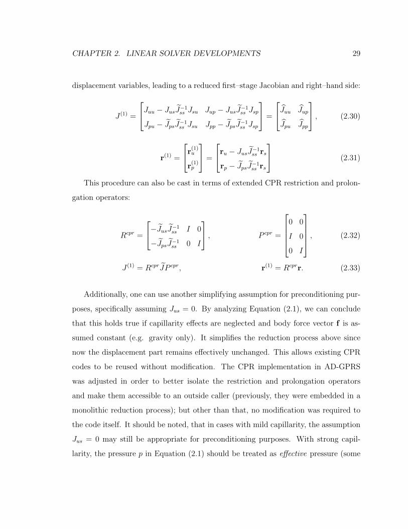
displacement variables, leading to a reduced first–stage Jacobian and right–hand side:

J (1) =

Juu − JusJ−1ss Jsu Jup − JusJ−1

ss Jsp

Jpu − JpsJ−1ss Jsu Jpp − JpsJ−1

ss Jsp

=

Juu Jup

Jpu Jpp

, (2.30)

r(1) =

r(1)u

r(1)p

=

ru − JusJ−1ss rs

rp − JpsJ−1ss rs

(2.31)

This procedure can also be cast in terms of extended CPR restriction and prolon-

gation operators:

Rcpr =

−JusJ−1ss I 0

−JpsJ−1ss 0 I

, P cpr =

0 0

I 0

0 I

, (2.32)

J (1) = RcprJP cpr, r(1) = Rcprr. (2.33)

Additionally, one can use another simplifying assumption for preconditioning pur-

poses, specifically assuming Jus = 0. By analyzing Equation (2.1), we can conclude

that this holds true if capillarity effects are neglected and body force vector f is as-

sumed constant (e.g. gravity only). It simplifies the reduction process above since

now the displacement part remains effectively unchanged. This allows existing CPR

codes to be reused without modification. The CPR implementation in AD-GPRS

was adjusted in order to better isolate the restriction and prolongation operators

and make them accessible to an outside caller (previously, they were embedded in a

monolithic reduction process); but other than that, no modification was required to

the code itself. It should be noted, that in cases with mild capillarity, the assumption

Jus = 0 may still be appropriate for preconditioning purposes. With strong capil-

larity, the pressure p in Equation (2.1) should be treated as effective pressure (some


form of average of phase pressures), and therefore a nonlinear saturation term would

enter the equation, giving rise to a non–trivial Jus.

In order to further decouple the system, an efficient preconditioner described by

[25] in the context of single–phase flow is employed, based on the fixed–stress concept.

The LDU decomposition of the first stage Jacobian reads:

J (1) = LDU =

I 0

JpuJ−1uu I

Juu 0

0 Spp

I J−1uu Jup

0 I

(2.34)

where Spp = Jpp − JpuJ−1uu Jup is a Schur complement with respect to Juu.

A variety of preconditioning operators can be constructed based on this decom-

position by preserving different factors. One particular choice is the upper triangular

operator:

P−1FS ≈ U−1D−1 =

J−1uu −J−1

uu JupS−1pp

0 S−1pp

(2.35)

where S−1pp ≈ P−1

p and J−1uu ≈ P−1

u are approximated using two nested preconditioners

for elliptic systems, such as multigrid methods. The algorithm for applying P−1FS to

a residual vector takes advantage of its block–triangular nature by first computing

the pressure components increment, δx(1)p , followed by the displacement components

increment, δx(1)u , as follows

δx(1)p = P−1

p r(1)p , δx(1)

u = P−1u (r(1)

u − Jupδx(1)p ). (2.36)


After that, the solution vectors are combined to arrive at the first stage solution:

δx(1) = P cpr

δx(1)u

δx(1)p

=

0

δx(1)u

δx(1)p

. (2.37)

Finally, following the CPR approach, a local second stage preconditioner P−1sm is

applied to the original system with an updated right-hand side, smoothing out the

high-frequency local error modes from the residual:

δx(2) = P−1sm(r− Jδx(1)), δx = δx(1) + δx(2). (2.38)

Different smoothing techniques can be applied in this stage. One approach is to

simply apply ILU or BILU family smoothers to the whole system, however, they are

not likely to be effective due to the block structure and high bandwidth of the matrix.

Based on the generalized block–partitioned preconditioner developed in the previous

section, another approach would be to employ a block Gauss-Seidel iteration with

separate BILU(0) or BILU(k) preconditioners on the flow/transport and mechanics

parts. This, however, can be expensive, as matrix of the mechanical part can be quite

large. One can note that the primary purpose of second stage is to smooth out the

errors caused by saturation advection, and in cases without a direct dependence of

displacement on saturation (such as when Jus = 0), second–stage updates to satura-

tion will not cause the displacement solution to change drastically. It can therefore

be beneficial to avoid the cost of constructing a factorization of geomechanical Ja-

cobian and simply apply smoothing to pressure and saturation/composition, bearing

the slight increase in iteration count.

Thus the overall scheme is a two–stage scheme with the first stage given by

the fixed–stress block algorithm, and second–stage given by either block–partitioned


Gauss-Seidel smoother, or a simple ILU smoother on the flow and transport part

only:

P−1CPR−FS = P−1

sm(I − JP−1FS) + P−1

FS (2.39)

Finally, a feasible way of constructing the Schur complement in Equation (2.34)

must be devised. Clearly, explicit construction of the full operator is infeasible due

to the size of matrices involved and high order of fill generated. Therefore, a cheap

and sparse approximation is sought. One possibility is implicit approximation by

evaluating the effect of triple product JpuJ−1uu Jup on vectors whenever required by the

outer Krylov solver. Here J−1uu can be approximated by the same preconditioning

operator P−1u used in the solution stage, or a different one. This, however, can

become prohibitively expensive with the cost of one extra invocation of P−1u per

Krylov iteration.

We consider a sparse approximation Spp that is constructed making use of the

fixed–stress split concept [13]. Following [25], Spp is explicitly computed from element–

wise contributions as a pressure space mass matrix scaled by a weighting factor de-

pending element–wise on the inverse of a suitable bulk modulus and Biot’s coefficient.

Note that this leads to a diagonal approximation Spp for a piecewise constant inter-

polation of the pressure field. As opposed to the original implementation [25], the

construction of Spp is here kept purely algebraic through the probing technique [18].

Denoting by e the probing vector, the diagonal approximation Spp is computed as:

Spp = Jpp − diag(JpuP−1u Jup · e), e = [1, 1, . . . , 1]T (2.40)

where diag() is a diagonal matrix created from elements of the argument vector. This

choice of approximation preserves row sums of the full operator by lumping elements

within a row into the diagonal. Note that here the Schur complement assembly is

only performed once per nonlinear iteration — or possibly per several, if the matrix


does not change significantly. In addition, the constructed P−1u is reused later in the

solution phase. Thus the extra cost of this approach, compared to, for instance, a

Gauss-Seidel type scheme, is equal to one application of P−1u and two matrix-vector

products. This cost is typically amortized across 10-30 Krylov iterations, and, as

indicated by numerical results, the convergence benefits outweigh the extra cost.

This completes the description of the preconditioner developed in this work. It’s

worth noting that the implementation of the strategy, including generating the Schur

approximation, is fairly straightforward in a framework with proper abstraction level,

i.e. where matrix–vector operations are well-defined and all preconditioning operators

have the same interface and can be treated as plug–in black–box solvers. The only

time where low–level access to matrix storage is required is update of the pressure

matrix diagonal elements while applying Schur complement.

Chapter 3

Numerical Examples

In order to assess the robustness and convergence of implemented preconditioners,

a number of test cases have been set up, including completely synthetic as well as

some derived from a well-known reservoir simulation benchmark SPE10 [5]. Here we

discuss the results.

The general setup of the linear solver used in this chapter is as follows. The outer

Krylov solver operating with a global coupled matrix is right–preconditioned GMRES

[18]. While other iterations, including Richardson, BiCGStab and left–preconditioned

GMRES, have been implemented, the focus here is on preconditioner efficiency; and

Richardson iteration is too slow or fails to converge in a reasonable amount of time in

some cases. The outer iteration runs with a convergence criteria of relative residual

reduction of τ = 10−10 and true, rather than preconditioned, residual norm is used

and reported. Additionally, GMRES is restarted every 100 iterations, and an overall

limit of 1500 iterations is set.

First–stage pressure preconditioner P−1p is one V–cycle of algebraic multigrid [22],

which is in practice enough to deal with long–range pressure error components for

preconditioning purposes. First–stage mechanics solver is another flavor of algebraic

34

CHAPTER 3. NUMERICAL EXAMPLES 35

multigrid, namely SAMG [21], well suited to non–scalar unknowns such as displace-

ment vectors. Here we use multigrid cycling in conjunction with a built-in BiCGStab

accelerator set to a loose tolerance of τu = 10−2, a value that provides a good balance

between quality of approximation of J−1uu and performance — experiments show that

using stricter tolerance does not provide enough overall convergence improvement

to offset the higher computational cost. The second stage employs a block version

of ILU(0) preconditioning, which is applied to the pressure–saturation system only.

Note that in the actual implementation the pressure and saturation unknowns are

not separated into δxp and δxs, but interleaved and ordered cell-wise. Thus the flow

and transport part of the Jacobian matrix is block-sparse with 2×2 dense blocks and

is naturally suited to Block-ILU smoothing.

All tests were performed on a system with a single quad-core Intel Core i7–4790

CPU and 16 GB of RAM. A single–threaded version of AD–GPRS, 2016 release, was

used for running simulations, linked with serial SAMG library.

3.1 Synthetic Flooding Problem

The first example is a poroelastic vertical slab of porous material initially saturated

with oil (with water at residual saturation) shown in Figure 3.1. The slab is flooded

with water from bottom to the top by subjecting its lower face to a fixed pressure

and saturation boundary condition. The upper face is kept at the initial pressure and

allowed to drain freely, while left and right faces are no-flow. Mechanically, the slab

is assigned a linear elastic behavior, with right, left and bottom faces prescribed zero

normal displacement, and top face allowed to deform. Both phases are slightly com-

pressible fluids with contrasting properties (namely, viscosity). Gravity and capillary

effects are neglected. Parameters of the system are summarized in Table 3.1.


Figure 3.1: Synthetic flooding test, model setup: (a) homogeneous permeability, (b)with low–permeability barriers, and (c) simulation coarse grid (h = 1 m).

Table 3.1: Synthetic flooding test, model parameters.

Domain size L×W ×H 10× 1× 10 m3

Young’s Modulus E 109 PaPoisson Ratio ν 0.25Biot Coefficient b 1.0Permeability k1 1 mDPermeability k2 0.001 mDTop Pressure p0 106 PaBottom Pressure p1 3× 106 PaFluid Compressibility cf 2× 10−10 Pa−1

Oil Viscosity µo 3 cPWater Viscosity µw 0.3 cP

We consider two cases: one with homogeneous permeability, and one with em-

bedded low-permeability barriers. Mechanical rock properties are kept homogeneous

in all cases. Geometry of the models and boundary conditions are displayed in Fig-

ure 3.1. A Cartesian grid with characteristic mesh size h is used to discretize the

domain. Table 3.2 reports problem space dimension for each of the grid sizes con-

sidered. Even though the problem is essentially 2–D (constant along y–axis), the

grid is refined in all 3 dimensions. For both cases the convergence behavior is ex-

amined for time step sizes ranging from 10−5 days to 1 day and a variety of grid


refinement levels. Convergence is compared between the combined Fixed–stress CPR

preconditioner (denoted as PFS) developed in Section 2.4 and a similar, but simpler

scheme, namely, a block Gauss-Seidel preconditioner (denoted by P−1GS) described in

Section 2.3.

Table 3.2: Synthetic flooding test, grid dimensions and problem size.

h [m] nx × ny × nz # cells # nodes # DOFs

1.0 10× 1× 10 120 286 1,0980.5 20× 2× 20 880 1,449 6,1070.25 40× 4× 40 6,720 8,815 39,8850.166 60× 6× 60 22,320 26,901 125,3430.125 80× 8× 80 52,480 60,507 286,4810.1 100× 10× 100 102,000 114,433 547,299

For each grid refinement level of both homogeneous and heterogeneous models,

and each time step size, 5 time steps were run, and the number of linear iterations

per Newton step was averaged across all nonlinear iterations of all time steps. Of

primary interest here is in the convergence behavior as a function of time step size

and grid block size. The expectation is that GMRES convergence with a good pre-

conditioning scheme should not degrade significantly with mesh refinement. Results

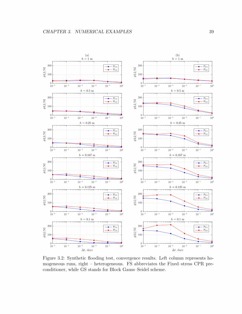
are summarized on Table 3.3 and presented visually in Figure 3.2.

These convergence results let us make the following observations. Using the Fixed–

stress CPR preconditioner has a clear advantage over a simpler block Gauss–Seidel

scheme, as it improves the iteration count by a factor of 1.5–3x over a wide range of

parameters. Time step size is an important factor here, since it affects the relative

scaling of flow/transport problem versus mechanics, and therefore the importance of

the Schur complement. Specifically, we observe that iteration count peaks at time

step sizes of 10−2–10−3 days; note that this is a fully synthetically scaled problem, so

the small time steps used in this test should not be dismissed as impractical. Grid


Table 3.3: Synthetic flooding test, average number of GMRES iterations per Newtonstep for the homogeneous permeability (a) and the low-permeability barriers case (b).

∆t [days] h [m] (a) (b)P−1FS P−1

GS P−1FS P−1

GS

1× 10−5 1.0 28 32.17 51.17 58.50.5 50 47 135.5 140.830.25 54.17 50.33 154.57 158.430.167 56 55.67 155.14 167.860.125 57.17 58 153.5 177.50.1 56 61.57 150.7 172.8

1× 10−4 1.0 28.6 33.6 54.17 61.50.5 49.8 47.8 133.5 143.50.25 50.5 51 144.75 1520.167 47.83 63 146.38 168.630.125 46 63.33 147.29 189.570.1 43.71 61.86 146.14 211.29

1× 10−3 1.0 32.67 37 56.71 600.5 42.83 46.5 117.57 139.570.25 37 48.75 136.83 1600.167 31.38 49.75 129.83 173.670.125 27.29 50.86 118 190.560.1 23.71 51.29 115.67 216.56

1× 10−2 1.0 33 35.14 46.67 48.50.5 28.43 38.43 82.71 105.140.25 18.67 38.67 99.4 132.10.167 14.67 37.5 78.64 1230.125 12 37.67 66.64 119.550.1 10.9 38.3 57.18 116.27

1× 10−1 1.0 20 22.14 35 38.290.5 13 22.29 49.9 58.20.25 9.4 23.2 41.09 55.820.167 8.27 21.82 32.18 53.820.125 7.82 22 26.64 53.180.1 7.73 21.55 24.08 54.08

1× 100 1.0 11 13.43 26.38 28.630.5 7.38 13.38 24.13 26.630.25 6.63 13 18.67 26.670.167 7 12.89 16 25.330.125 8.1 12.89 12.75 25.890.1 8.6 12.44 12.92 26.63


10−5 10−4 10−3 10−2 10−1 1000

100

200

#LI/NI

(a)h = 1 m

PFS

PGS

10−5 10−4 10−3 10−2 10−1 1000

100

200

#LI/NI

(b)h = 1 m

PFS

PGS

10−5 10−4 10−3 10−2 10−1 1000

100

200

#LI/NI

h = 0.5 m

PFS

PGS

10−5 10−4 10−3 10−2 10−1 1000

100

200

#LI/NI

h = 0.5 m

PFS

PGS

10−5 10−4 10−3 10−2 10−1 1000

100

200

#LI/NI

h = 0.25 m

PFS

PGS

10−5 10−4 10−3 10−2 10−1 1000

100

200

#LI/NI

h = 0.25 m

PFS

PGS

10−5 10−4 10−3 10−2 10−1 1000

100

200

#LI/NI

h = 0.167 m

PFS

PGS

10−5 10−4 10−3 10−2 10−1 1000

100

200

#LI/NI

h = 0.167 m

PFS

PGS

10−5 10−4 10−3 10−2 10−1 1000

100

200

#LI/NI

h = 0.125 m

PFS

PGS

10−5 10−4 10−3 10−2 10−1 1000

100

200

#LI/NI

h = 0.125 m

PFS

PGS

10−5 10−4 10−3 10−2 10−1 100

∆t, days

0

100

200

#LI/NI

h = 0.1 m

PFS

PGS

10−5 10−4 10−3 10−2 10−1 100

∆t, days

0

100

200

#LI/NI

h = 0.1 m

PFS

PGS

Figure 3.2: Synthetic flooding test, convergence results. Left column represents ho-mogeneous runs, right – heterogeneous. FS abbreviates the Fixed–stress CPR pre-conditioner, while GS stands for Block Gauss–Seidel scheme.


refinement amplifies the effect, with the difference being barely noticeable on smaller

grids and growing with the number of cells. Note that both solution algorithms suffer

an initial increase in iteration count as the grid is refined 2 and 4 times; however, after

that point the convergence of PFS stabilizes, while for PGS it continues to degrade all

the way until the finest 100k cell grid (and is expected to continue to degrade with

more refinement), making this approach infeasible on large grids.

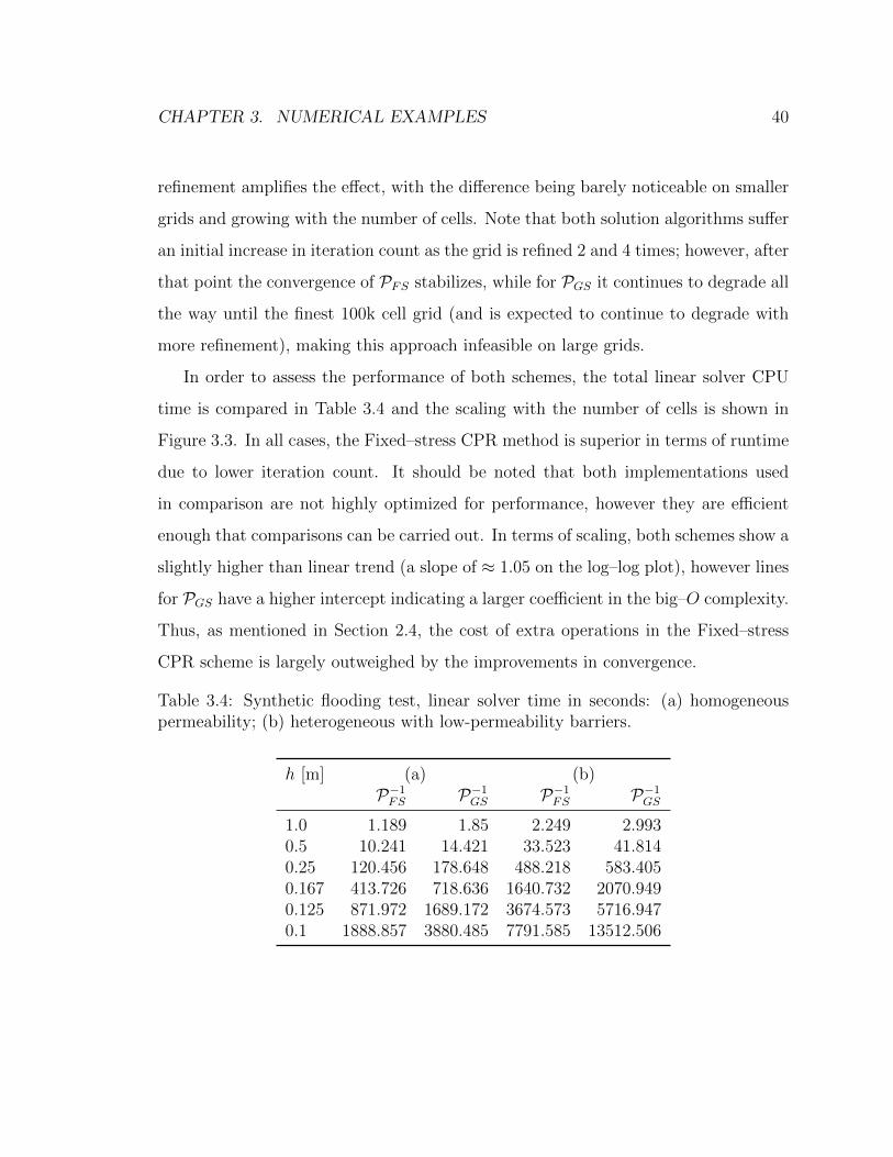
In order to assess the performance of both schemes, the total linear solver CPU

time is compared in Table 3.4 and the scaling with the number of cells is shown in

Figure 3.3. In all cases, the Fixed–stress CPR method is superior in terms of runtime

due to lower iteration count. It should be noted that both implementations used

in comparison are not highly optimized for performance, however they are efficient

enough that comparisons can be carried out. In terms of scaling, both schemes show a

slightly higher than linear trend (a slope of ≈ 1.05 on the log–log plot), however lines

for PGS have a higher intercept indicating a larger coefficient in the big–O complexity.

Thus, as mentioned in Section 2.4, the cost of extra operations in the Fixed–stress

CPR scheme is largely outweighed by the improvements in convergence.

Table 3.4: Synthetic flooding test, linear solver time in seconds: (a) homogeneouspermeability; (b) heterogeneous with low-permeability barriers.

h [m] (a) (b)P−1FS P−1

GS P−1FS P−1

GS

1.0 1.189 1.85 2.249 2.9930.5 10.241 14.421 33.523 41.8140.25 120.456 178.648 488.218 583.4050.167 413.726 718.636 1640.732 2070.9490.125 871.972 1689.172 3674.573 5716.9470.1 1888.857 3880.485 7791.585 13512.506


102 103 104 105

# cells

100

101

102

103

104

105

Totallinearsolver

time,

s

Homogeneous, PFS

Homogeneous, PGS

Heterogeneous, PFS

Heterogeneous, PGS

Figure 3.3: Synthetic flooding test, scaling results.

3.2 SPE10–Based Reservoir

Here we consider a more realistic problem setup and demonstrate that the proposed

approach can be applied robustly to modeling multiphase reservoir flow with geome-

chanical effects. The test case is based on the SPE10 porosity and permeability fields,

from which the top 32 layers have been extracted and additionally upscaled 2 and 4

times in each direction. Upscaling has been performed using the open–source MAT-

LAB Reservoir Simulation Toolbox [16]. The sizes of each model are summarized in

Table 3.5, displayed in Figure 3.4. The permeability field is characterized by high

degrees of heterogeneity and anisotropy — although to a lesser degree in upscaled

versions — and is generally considered to present a challenge for solvers.

The model is additionally equipped with poroelastic mechanical behavior with

homogeneous properties. All boundaries are constrained to have zero normal dis-

placement, except for the top one which is allowed to deform freely. The relevant


Table 3.5: SPE10–based test, grid dimensions and problem size.

nx × ny × nz # cells # nodes # DOFs

15× 55× 8 6,600 8,064 37,39230× 110× 16 52,800 58,497 281,09160× 220× 32 422,400 444,873 2,179,419

Figure 3.4: Permeability fields for SPE10-based test case: kx, ky (top row), kz (bottomrow).

physical parameters are summarized in Table 3.6. Multiphase dynamics is intro-

duced by a pair of producing and water-injecting wells located in opposite corners

of the domain (mimicking a quarter 5-spot) and penetrating all layers. Both wells

are operating at constant bottom hole pressure, creating a pressure gradient across

the reservoir that drives the flow and leads to formation compaction in some parts of

the reservoir and formation expansion in others. This reservoir behavior cannot be

correctly captured by using a simple uniaxial rock compressibility parameter due to

boundary condition effects, however it can have a significant impact on production

at early times. Thus having an efficient and robust coupled solver can be beneficial.


Table 3.6: SPE10-based reservoir: model parameters.

Domain size L×W ×H 120× 220× 6.4 m3

Young’s Modulus E 3.1 GPaPoisson Ratio ν 0.2Biot Coefficient b 0.8Injection Pressure pinj 50 MPaInitial Pressure pinit 30 MPaProduction Pressure pprod 10 MPaFluid Compressibility cf 4.35× 10−10 Pa−1

Oil Viscosity µo 3 cPWater Viscosity µw 0.3 cP

3.2.1 Convergence

Figure 3.5 shows convergence of FS–CPR preconditioned GMRES on the fine and

upscaled grids for a variety of time step sizes. Convergence history was collected

from the second Newton iteration of the first repetition of each time step size (the

first Newton iteration is skipped as the matrix does not include an accumulation term

and thus is not representative of most matrices the solver has to deal with during the

course of the simulation). Generally it can be observed that for all except the largest

(100 and 1000 days) time step sizes the linear solver reduces the residual by 10 orders

of magnitude within 20-25 iterations; for large time step sizes this number is between

40 and 50 for large grids. It might seem like convergence deteriorates with increasing

grid size, however, this is more likely to be the effect of upscaling, which tends to

make the upscaled grids less heterogeneous and anisotropic, and thus less challenging

for the solver. Thus we conclude that the proposed FS–CPR scheme can be reliably

applied to more realistic reservoir modeling problems with a range of time step sizes.

Note that even though pressure-displacement coupling strength is quite mild in this

example and a simpler preconditioner might be sufficient, as mentioned previously,

the FS–CPR scheme comes at only a small extra computational cost and therefore


can be viewed as a universally applicable preconditioner for problems with coupled

multiphase flow and mechanics.

0 10 20 30 40 50

GMRES iteration

10−10

10−8

10−6

10−4

10−2

100

||r k||2/||r

0||2

15× 55× 8

∆t = 10−3

∆t = 10−2

∆t = 10−1

∆t = 100

∆t = 101

∆t = 102

∆t = 103

0 10 20 30 40 50

GMRES iteration

10−10

10−8

10−6

10−4

10−2

100

||r k||2/||r

0||2

30× 110× 16

∆t = 10−3

∆t = 10−2

∆t = 10−1

∆t = 100

∆t = 101

∆t = 102

∆t = 103

0 10 20 30 40 50

GMRES iteration

10−10

10−8

10−6

10−4

10−2

100

||r k||2/||r

0||2

60× 220× 32

∆t = 10−3

∆t = 10−2

∆t = 10−1

∆t = 100

∆t = 101

∆t = 102

∆t = 103

Figure 3.5: SPE10–based test, convergence on fine and upscaled grids. Time stepsizes are in days.

3.2.2 Effect of capillarity

Additionally, we investigate the effect of capillary pressure on linear convergence. As

was explained in Section 2.4, in the current implementation the block Jus is ignored,

even though it can be present in presence of capillarity, since the effective pressure


p in Equation (2.1) is usually computed as volume (saturation) averaged fluid phase

pressure:

peff =

Np∑p=1

Sppp (3.1)

where

pp = pw + pc(Sp) (3.2)

with w being the wetting phase. Thus the derivatives of Equation (2.1) with respect to

saturation unknowns, which make up Jus, are generally nonzero, and it is desirable to

both better understand the limitations of current implementation and justify investing

additional effort in the proper treatment of Jus. We use the smallest 15× 55× 8 grid

to investigate this, and the imbibition capillary pressure is modeled after [14] as:

pc = pmaxc (1− S∗w)m (3.3)

where m = 4 is chosen and pmaxc is varied to derive models with different capillarity

pressure curves. Figure 3.6 shows the GMRES convergence plots for different time

step sizes and capillarity strength. It is immediately clear that for large enough

time step sizes increasing capillary pressure severely affects convergence of the FS–

CPR scheme. In order to assess whether this happens due to neglecting the Jus

Jacobian contributions in the CPR–FS implementation or simply by the virtue of

CPR stagnation with capillarity (due to the appearance of a diffusion–like saturation

term that is not handled efficiently by the scheme), the same simulations were run

with mechanics disabled, using the default CPR preconditioner. The results of these

runs are shown in Figure 3.7, in the same format as Figure 3.6. The fact that

convergence curves look almost exactly identical to the CPR–FS ones hints that the

effect of capillarity on CPR completely dominates any convergence losses stemming

from approximate Jacobian treatment in CPR–FS. In addition, Figure 3.8 shows


the ratio of linear iteration count required by the two operators in their respective

simulation runs. For smaller time step sizes CPR–FS takes a lot more iterations as

it has to resolve the errors in mechanical solution (these time steps are taken in the

beginning of simulation, when mechanical deformation is still ongoing), but for larger

time steps the two operators very similar convergence. However, these results are not

conclusive enough and a more in–depth investigation of this issue is in order.

0 10 20 30 40 50

GMRES iteration

10−10

10−8

10−6

10−4

10−2

100

||r k||2/||r

0||2

∆t = 100 days

pmaxc = 0 bar

pmaxc = 2 bar

pmaxc = 5 bar

0 10 20 30 40 50

GMRES iteration

10−10

10−8

10−6

10−4

10−2

100

||r k||2/||r

0||2

∆t = 101 days

pmaxc = 0 bar

pmaxc = 2 bar

pmaxc = 5 bar

0 10 20 30 40 50

GMRES iteration

10−10

10−8

10−6

10−4

10−2

100

||r k||2/||r

0||2

∆t = 102 days

pmaxc = 0 bar

pmaxc = 2 bar

pmaxc = 5 bar

0 10 20 30 40 50

GMRES iteration

10−10

10−8

10−6

10−4

10−2

100

||r k||2/||r

0||2

∆t = 103 days

pmaxc = 0 bar

pmaxc = 2 bar

pmaxc = 5 bar

Figure 3.6: SPE10–based test, influence of capillarity on convergence. The linesoverlap on top left plot (∆t = 1 day).


0 10 20 30 40 50

GMRES iteration

10−10

10−8

10−6

10−4

10−2

100

||r k||2/||r

0||2

∆t = 100 days, no mechanics

pmaxc = 0 bar

pmaxc = 2 bar

pmaxc = 5 bar

0 10 20 30 40 50

GMRES iteration

10−10

10−8

10−6

10−4

10−2

100

||r k||2/||r

0||2


pmaxc = 0 bar

pmaxc = 2 bar

pmaxc = 5 bar

0 10 20 30 40 50

GMRES iteration

10−10

10−8

10−6

10−4

10−2

100

||r k||2/||r

0||2


pmaxc = 0 bar

pmaxc = 2 bar

pmaxc = 5 bar

0 10 20 30 40 50

GMRES iteration

10−10

10−8

10−6

10−4

10−2

100

||r k||2/||r

0||2


pmaxc = 0 bar

pmaxc = 2 bar

pmaxc = 5 bar

Figure 3.7: SPE10–based test without mechanics, influence of capillarity on conver-gence. The lines overlap on top left plot (∆t = 1 day).


10−3 10−2 10−1 100 101 102 103

∆t, days

0.5

1

1.5

2

2.5

3

3.5

4

#LICPR-FS/#LICPR

Linear convergence of CPR-FS vs. CPR

pmaxc = 0 bar

pmaxc = 2 bar

pmaxc = 5 bar

Figure 3.8: SPE10–based test, ratio of the number of linear iterations taken by CPR–FS vs. CPR scheme for a range of time steps and varying capillarity strength.

Chapter 4

Concluding Remarks

4.1 Conclusions

In present work the problem of achieving an efficient fully implicit solution of coupled

multiphase flow and poromechanics has been tackled. A well implemented fully im-

plicit simulator for a certain range of parameters may outperform sequential implicit

schemes, since solution is achieved via an efficient Krylov subspace solver, rather than

a fixed–point iteration that in the linear limit is equivalent to a Richardson scheme

[25]. The linear systems arising during solution naturally possess a block structure

and the major difficulty is the construction of a robust preconditioning operator, since

simple preconditioners, such as ILU, are not sufficient. Such an operator has been

constructed through an effective combination of the Constrained Pressure Residual

preconditioner with the fixed–stress block-partitioned scheme. In order to deliver an

efficient implementation within the research reservoir simulator AD–GPRS, existing

data structures have been adapted and extended to handle fully implicit Jacobians

with mechanics, while also laying the groundwork for a fully flexible linear solver plat-

form in which specialized multiphysics preconditioners can be built and experimented

with. In addition to the FS–CPR scheme for mechanics, a generic block–partitioned

49

CHAPTER 4. CONCLUDING REMARKS 50

preconditioner that works via a Jacobi or Gauss-Seidel iteration has been implemented

as a base building block for more complex schemes involving additional physics. The

performance of both has been evaluated using a synthetically constructed and refined

waterflooding problem, which revealed that the FS–CPR scheme outperforms simpler

block–partitioned approaches and scales well by retaining constant iteration count as

the number of grid elements is increased. Additionally, it has been applied to a more

realistic waterflooding production scenario involving an SPE10–based permeability

and porosity fields with added mechanical behavior. The preconditioner works reli-

ably in absence of strong capillarity, however more effort is required to adapt it to

capillarity by augmenting both the CPR and CPR–FS strategies with proper treat-

ment of the capillary pressure terms and respective Jacobian blocks.

4.2 Future Work

While these initial results are very promising, a lot more needs to be done to achieve

a fully robust linear solver. An obvious continuation of this work is to implement

proper treatment of capillarity. Aside from that, it is quite important to investi-

gate the relative impact of different kernels (pressure and mechanics solvers, second

stage smoother) and tune their parameters (multigrid cycles, tolerances and other) to

achieve maximum performance. More rigorous testing is required as well, including

unstructured grids and heterogeneous mechanical properties, as well as performing

3–phase and/or compositional simulations to better assess the impact of multiphase

physics on solver performance. Finally, building on the framework that is being devel-

oped for scalable multistage multiphysics preconditioning, advanced solution schemes

for multiple fully coupled problems, such as thermo–hydro–mechanics, can be devel-

oped, incorporating ideas from sequential implicit operator splitting schemes. With

CHAPTER 4. CONCLUDING REMARKS 51

additional effort invested in building specialized linear solvers, the fully implicit ap-

proach may become the method of choice for many multiphysics problems, especially

ones that exhibit strong coupling.

Bibliography

[1] J. Bear. Dynamics of Fluids in Porous Media. Dover, 1972.

[2] H. Cao. Development of Techniques for General Purpose Simulators. PhD thesis,

Stanford University, 2002.

[3] H. Cao, H.A. Tchelepi, J.R. Wallis, and H.E. Yardumian. Parallel scalable un-

structured cpr-type linear solver for reservoir simulation. In Proceedings - SPE

Annual Technical Conference and Exhibition, Dallas, TX, 2005.

[4] N. Castelletto, J.A. White, and Tchelepi H.A. A unified framework for fully-

implicit and sequential-implicit schemes for coupled poroelasticity. In Proceed-

ings, ECMOR XIV - 14th European conference on the mathematics of oil recov-

ery. Catania, Italy, 2014.

[5] M. A. Christie and M. J. Blunt. Tenth spe comparative solution project: A

comparison of upscaling techniques. SPE Reservoir Evaluation and Engineering,

4(04):308–317, 2001.

[6] O. Coussy. Poromechanics. John Wiley & Sons Ltd, Chichester, UK, 2004.

[7] R. H. Dean, X. Gai, C. M. Stone, and S. E. Minkoff. A Comparison of Techniques

for Coupling Porous Flow and Geomechanics. SPE Journal, 11(01):132–140,

2006.

52

BIBLIOGRAPHY 53

[8] James W. Demmel, Stanley C. Eisenstat, John R. Gilbert, Xiaoye S. Li, and

Joseph W. H. Liu. A supernodal approach to sparse partial pivoting. SIAM J.

Matrix Analysis and Applications, 20(3):720–755, 1999.

[9] E. Fjaer, R.M. Holt, P. Horsrud., A.M. Raaen, and Risnes R. Petroleum Related

Rock Mechanics. Elsevier, Amsterdam and Oxford, 2nd edition, 2008.

[10] Y. Jiang. Techniques for Modeling Complex Reservoirs and Advanced Wells.

PhD thesis, Stanford University, 2007.

[11] J. Kim. Sequential Methods for Coupled Geomechanics and Multiphase Flow.

PhD thesis, Stanford University, 2010.

[12] Jihoon Kim, Hamdi A. Tchelepi, and Ruben Juanes. Stability, accuracy and

efficiency of sequential methods for coupled flow and geomechanics. SPE Journal,

16(2):249–262, 2011.

[13] Jihoon Kim, Hamdi A. Tchelepi, and Ruben Juanes. Stability and convergence

of sequential methods for coupled flow and geomechanics: Fixed-stress and fixed-

strain splits. Computer Methods in Applied Mechanics and Engineering, 200(13-

16):1591–1606, 2011.

[14] K. Li and R. N. Horne. An experimental and analytical study of steam/water

capillary pressure. SPE Reservoir Evaluation and Engineering, 4(06):477–482,

2001.

[15] X.S. Li, J.W. Demmel, J.R. Gilbert, iL. Grigori, M. Shao, and I. Yamazaki.

SuperLU Users’ Guide. Technical Report LBNL–44289, Lawrence Berkeley Na-

tional Laboratory, September 1999. http://crd.lbl.gov/~xiaoye/SuperLU/.

Last update: August 2011.

http://crd.lbl.gov/~xiaoye/SuperLU/

BIBLIOGRAPHY 54

[16] Knut-Andreas Lie, Stein Krogstad, Ingeborg Skjelkvale Ligaarden, Jostein Roald

Natvig, Halvor Møll Nilsen, and Bard Skaflestad. Open-source matlab implemen-

tation of consistent discretisations on complex grids. Computational Geosciences,

16(2):297–322, 2012.

[17] D. W. Peaceman. Interpretation of well–block pressures in numerical reservoir

simulation. SPE Journal, 18(03):183–194, 1978.

[18] Y. Saad. Iterative Methods for Sparse Linear Systems. SIAM, Philadelphia,

USA, 2003.

[19] Youcef Saad and Martin H Schultz. Gmres: A generalized minimal residual

algorithm for solving nonsymmetric linear systems. SIAM J. Sci. Stat. Comput.,

7(3):856–869, July 1986.

[20] O. Schenk and K. Gartner. Solving unsymmetric sparse systems of linear equa-

tions with paradiso. Future Generation Computer Systems, 20(3):475–487, apr

2004.

[21] K. Stuben. SAMG User’s Manual. Fraunhofer SCAI, 2012.

[22] Klaus Stuben. Algebraic multigrid (amg): experiences and comparisons. Applied

mathematics and computation, 13(3):419–451, 1983.

[23] D. Voskov and Y. Zhou. Technical description of AD-GPRS. Energy Resources

Engineering, Stanford University, 2012.

[24] John Wallis. Incomplete gaussian elimination as a preconditioning for general-

ized conjugate gradient acceleration. In Proceedings of the 7th SPE Reservoir

Simulation Symposium, San Francisco, CA, 1983.

BIBLIOGRAPHY 55

[25] J. A. White, N. Castelletto, and H. A. Tchelepi. Block-partitioned solvers for

coupled poromechanics: A unified framework. Comput. Meth. Appl. Mech. Eng.,

303:55–74, 2016.

[26] R.M. Younis. Modern advances in software and solution algorithms for reservoir

simulation. PhD thesis, Stanford University, 2011.

[27] Y. Zhou. Multistage preconditioner for well groups and automatic differentiation

for next generation gprs. Master’s thesis, Stanford University, 2009.

[28] Y. Zhou. Parallel General-Purpose Reservoir Simulation with Coupled Reservoir

Models and Multisegment Wells. PhD thesis, Stanford University, 2012.

Linear Solution Techniques for Reservoir Simulation · PDF filelinear solution techniques for...

Documents

Transcript of Linear Solution Techniques for Reservoir Simulation · PDF filelinear solution techniques for...