Linear Regression Example Data House Price in $1000s (Y) Square Feet (X) 2451400 3121600 2791700...
43
Linear Regression Example Data House Price in $1000s (Y) Square Feet (X) 245 1400 312 1600 279 1700 308 1875 199 1100 219 1550 405 2350 324 2450 319 1425 255 1700 Statistics for Managers Using Microsoft Excel, 5e © 2008 Prentice-Hall, Inc. Chap 13-1
-
Upload
laurel-little -
Category
Documents
-
view
213 -
download
0
Transcript of Linear Regression Example Data House Price in $1000s (Y) Square Feet (X) 2451400 3121600 2791700...
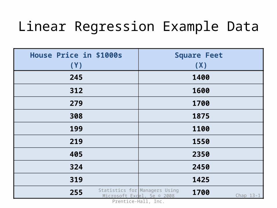
Linear Regression Example DataHouse Price in $1000s
(Y)Square Feet
(X)
245 1400
312 1600
279 1700
308 1875
199 1100
219 1550
405 2350
324 2450
319 1425
255 1700
Statistics for Managers Using Microsoft Excel, 5e © 2008 Prentice-Hall, Inc. Chap 13-1
Statistics for Managers Using Microsoft Excel, 5e © 2008 Prentice-Hall, Inc. Chap 13-2
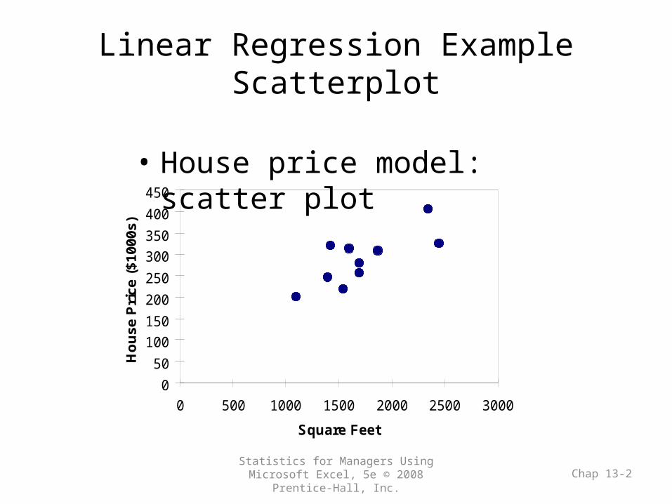
Linear Regression ExampleScatterplot
0
50
100
150
200
250
300
350
400
450
0 500 1000 1500 2000 2500 3000
Square Feet
Ho
use
Pri
ce (
$100
0s)
• House price model: scatter plot
Statistics for Managers Using Microsoft Excel, 5e © 2008 Prentice-Hall, Inc. Chap 13-3
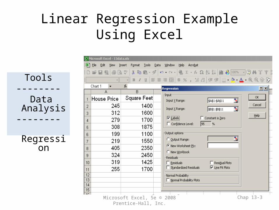
Linear Regression ExampleUsing Excel
Tools--------
Data Analysis--------
Regression

Statistics for Managers Using Microsoft Excel, 5e © 2008 Prentice-Hall, Inc. Chap 13-4
Linear Regression ExampleExcel Output
Regression Statistics
Multiple R 0.76211
R Square 0.58082
Adjusted R Square 0.52842
Standard Error 41.33032
Observations 10
ANOVA df SS MS F Significance F
Regression 1 18934.9348 18934.9348 11.0848 0.01039
Residual 8 13665.5652 1708.1957
Total 9 32600.5000
Coefficients Standard Error t Stat P-value Lower 95% Upper 95%
Intercept 98.24833 58.03348 1.69296 0.12892 -35.57720 232.07386
Square Feet 0.10977 0.03297 3.32938 0.01039 0.03374 0.18580
The regression equation is:feet) (square 0.10977 98.24833 price house
Statistics for Managers Using Microsoft Excel, 5e © 2008 Prentice-Hall, Inc. Chap 13-5
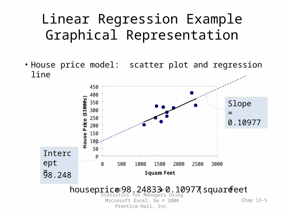
Linear Regression ExampleGraphical Representation
0
50
100
150
200
250
300
350
400
450
0 500 1000 1500 2000 2500 3000
Square Feet
Ho
use
Pri
ce (
$100
0s)
• House price model: scatter plot and regression line
feet) (square 0.10977 98.24833 price house
Slope = 0.10977
Intercept = 98.248

Statistics for Managers Using Microsoft Excel, 5e © 2008 Prentice-Hall, Inc. Chap 13-6
Linear Regression ExampleInterpretation of b0
• b0 is the estimated mean value of Y when the value of X is zero (if X = 0 is in the range of observed X values)
• Because the square footage of the house cannot be 0, the Y intercept has no practical application.
feet) (square 0.10977 98.24833 price house

Statistics for Managers Using Microsoft Excel, 5e © 2008 Prentice-Hall, Inc. Chap 13-7
Linear Regression ExampleInterpretation of b1
• b1 measures the mean change in the average value of Y as a result of a one-unit change in X
• Here, b1 = .10977 tells us that the mean value of a house increases by .10977($1000) = $109.77, on average, for each additional one square foot of size
feet) (square 0.10977 98.24833 price house
Statistics for Managers Using Microsoft Excel, 5e © 2008 Prentice-Hall, Inc. Chap 13-8
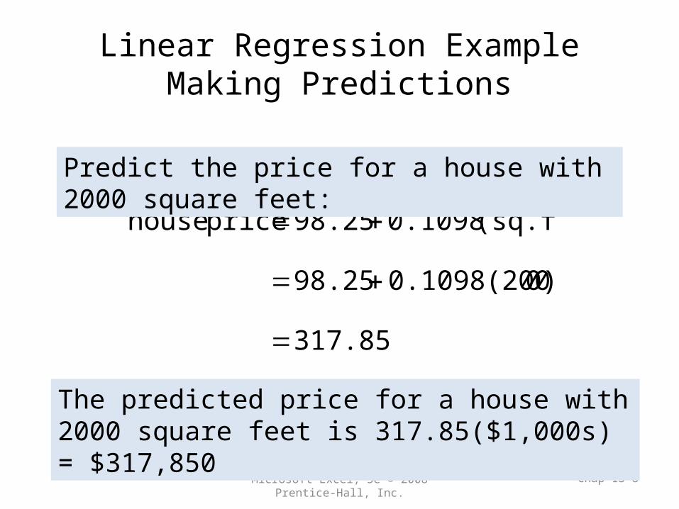
Linear Regression ExampleMaking Predictions
317.85
0)0.1098(200 98.25
(sq.ft.) 0.1098 98.25 price house
Predict the price for a house with 2000 square feet:
The predicted price for a house with 2000 square feet is 317.85($1,000s) = $317,850

Statistics for Managers Using Microsoft Excel, 5e © 2008 Prentice-Hall, Inc. Chap 13-9
Linear Regression ExampleMaking Predictions
0
50
100
150
200
250
300
350
400
450
0 500 1000 1500 2000 2500 3000
Square Feet
Ho
use
Pri
ce (
$100
0s)
• When using a regression model for prediction, only predict within the relevant range of data
Relevant range for interpolation
Do not try to extrapolate beyond
the range of observed X’s

Statistics for Managers Using Microsoft Excel, 5e © 2008 Prentice-Hall, Inc. Chap 13-10
Measures of Variation
Total variation is made up of two parts:
SSE SSR SST Total Sum of Squares
Regression Sum of Squares
Error Sum of Squares
2i )YY(SST 2
ii )YY(SSE 2i )YY(SSR
where:
= Mean value of the dependent variable
Yi = Observed values of the dependent variable
i = Predicted value of Y for the given Xi valueY
Y

Statistics for Managers Using Microsoft Excel, 5e © 2008 Prentice-Hall, Inc. Chap 13-11
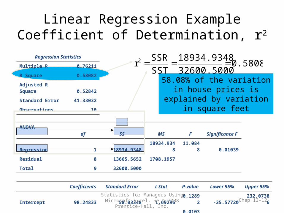
Coefficient of Determination, r2
• The coefficient of determination is the portion of the total variation in the dependent variable that is explained by variation in the independent variable
• The coefficient of determination is also called r-squared and is denoted as r2
1r0 2
squares of sum total
squares of sum regression
SST
SSRr2
Regression Statistics
Multiple R 0.76211
R Square 0.58082
Adjusted R Square 0.52842
Standard Error 41.33032
Observations 10
ANOVA df SS MS F Significance F
Regression 1 18934.9348 18934.9348 11.0848 0.01039
Residual 8 13665.5652 1708.1957
Total 9 32600.5000
Coefficients Standard Error t Stat P-value Lower 95% Upper 95%
Intercept 98.24833 58.03348 1.69296 0.12892 -35.57720 232.07386
Square Feet 0.10977 0.03297 3.32938 0.01039 0.03374 0.18580
Statistics for Managers Using Microsoft Excel, 5e © 2008 Prentice-Hall, Inc. Chap 13-12
Linear Regression ExampleCoefficient of Determination, r2
58.08% of the variation in house prices is explained by variation in
square feet
0.5808232600.5000
18934.9348
SST
SSRr2

Statistics for Managers Using Microsoft Excel, 5e © 2008 Prentice-Hall, Inc. Chap 13-13
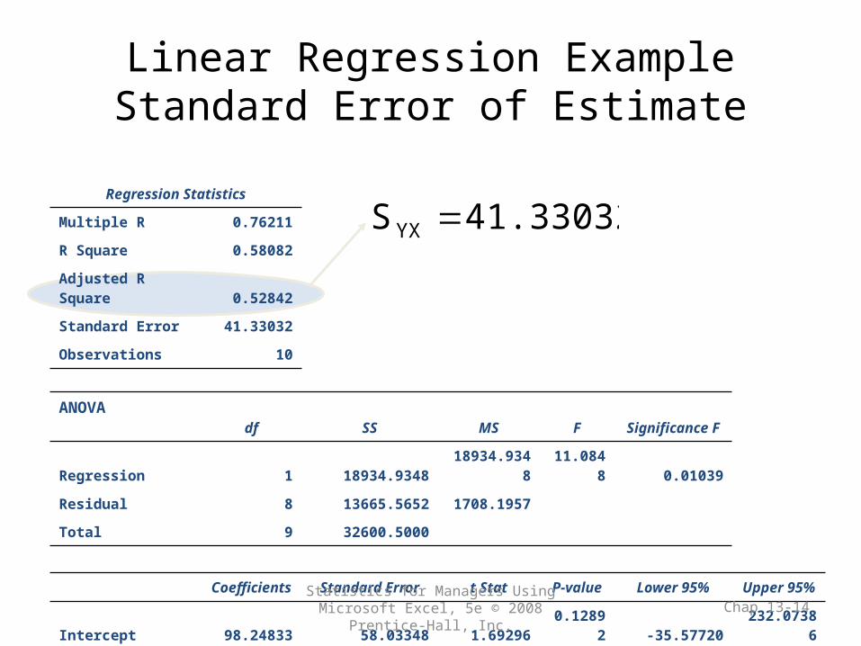
Standard Error of Estimate
• The standard deviation of the variation of observations around the regression line is estimated by
2
)ˆ(
21
2
n
YY
n
SSES
n
iii
YX
WhereSSE = error sum of squares n = sample size
Regression Statistics
Multiple R 0.76211
R Square 0.58082
Adjusted R Square 0.52842
Standard Error 41.33032
Observations 10
ANOVA df SS MS F Significance F
Regression 1 18934.9348 18934.9348 11.0848 0.01039
Residual 8 13665.5652 1708.1957
Total 9 32600.5000
Coefficients Standard Error t Stat P-value Lower 95% Upper 95%
Intercept 98.24833 58.03348 1.69296 0.12892 -35.57720 232.07386
Square Feet 0.10977 0.03297 3.32938 0.01039 0.03374 0.18580
Statistics for Managers Using Microsoft Excel, 5e © 2008 Prentice-Hall, Inc. Chap 13-14
Linear Regression ExampleStandard Error of Estimate
41.33032SYX
Statistics for Managers Using Microsoft Excel, 5e © 2008 Prentice-Hall, Inc. Chap 13-15
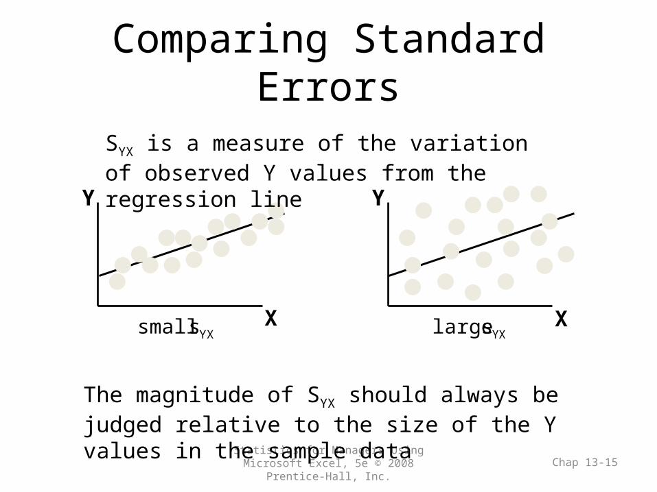
Comparing Standard Errors
YY
X XYXs small YXs large
SYX is a measure of the variation of observed Y values from the regression line
The magnitude of SYX should always be judged relative to the size of the Y values in the sample data
Statistics for Managers Using Microsoft Excel, 5e © 2008 Prentice-Hall, Inc. Chap 13-16
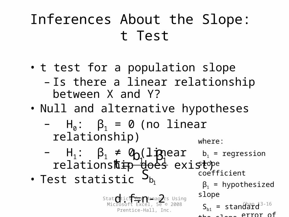
Inferences About the Slope: t Test
• t test for a population slope– Is there a linear relationship between X and Y?
• Null and alternative hypotheses– H0: β1 = 0 (no linear relationship)– H1: β1 ≠ 0 (linear relationship does exist)
• Test statistic
1b
11
S
βbt
2nd.f.
where:
b1 = regression slope coefficient
β1 = hypothesized slope
Sb1 = standard error of the slope

Statistics for Managers Using Microsoft Excel, 5e © 2008 Prentice-Hall, Inc. Chap 13-17
Inferences About the Slope: t Test Example
House Price in $1000s
(y)
Square Feet (x)
245 1400
312 1600
279 1700
308 1875
199 1100
219 1550
405 2350
324 2450
319 1425
255 1700
(sq.ft.) 0.1098 98.25 price house
Estimated Regression Equation:
The slope of this model is 0.1098
Is there a relationship between the square footage of the house and its sales price?

Statistics for Managers Using Microsoft Excel, 5e © 2008 Prentice-Hall, Inc. Chap 13-18
Inferences About the Slope: t Test Example
• H0: β1 = 0
• H1: β1 ≠ 0
From Excel output: Coefficients Standard Error t Stat P-value
Intercept 98.24833 58.03348 1.69296 0.12892
Square Feet 0.10977 0.03297 3.32938 0.01039
1bS
t
b1
32938.303297.0
010977.0
S
βbt
1b
11

Statistics for Managers Using Microsoft Excel, 5e © 2008 Prentice-Hall, Inc. Chap 13-19
Inferences About the Slope: t Test Example
Test Statistic: t = 3.329
There is sufficient evidence that square footage affects house price
Decision: Reject H0
Reject H0Reject H0
a/2=.025
-tα/2Do not reject H0
0 tα/2
a/2=.025
-2.3060 2.3060 3.329
d.f. = 10- 2 = 8
• H0: β1 = 0
• H1: β1 ≠ 0

Statistics for Managers Using Microsoft Excel, 5e © 2008 Prentice-Hall, Inc. Chap 13-20
Inferences About the Slope: t Test Example
• H0: β1 = 0
• H1: β1 ≠ 0
From Excel output: Coefficients Standard Error t Stat P-value
Intercept 98.24833 58.03348 1.69296 0.12892
Square Feet 0.10977 0.03297 3.32938 0.01039
P-Value
There is sufficient evidence that square footage affects house price.
Decision: Reject H0, since p-value < α

Statistics for Managers Using Microsoft Excel, 5e © 2008 Prentice-Hall, Inc. Chap 13-21
F-Test for Significance
• F Test statistic:
where
MSE
MSRF
1kn
SSEMSE
k
SSRMSR
where F follows an F distribution with k numerator degrees of freedom and (n - k - 1) denominator degrees of freedom
(k = the number of independent variables in the regression model)
Statistics for Managers Using Microsoft Excel, 5e © 2008 Prentice-Hall, Inc. Chap 13-22
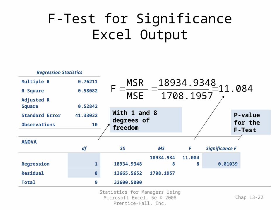
F-Test for SignificanceExcel Output
Regression Statistics
Multiple R 0.76211
R Square 0.58082
Adjusted R Square 0.52842
Standard Error 41.33032
Observations 10
ANOVA df SS MS F Significance F
Regression 1 18934.9348 18934.9348 11.0848 0.01039
Residual 8 13665.5652 1708.1957
Total 9 32600.5000
11.08481708.1957
18934.9348
MSE
MSRF
With 1 and 8 degrees of freedom
P-value for the F-Test

Statistics for Managers Using Microsoft Excel, 5e © 2008 Prentice-Hall, Inc. Chap 13-23
F-Test for Significance
• H0: β1 = 0
• H1: β1 ≠ 0• = .05• df1= 1 df2 = 8
Test Statistic:
Decision:
Conclusion:
Reject H0 at = 0.05
There is sufficient evidence that house size affects selling price0
= .05
F.05 = 5.32Reject H0Do not
reject H0
11.08MSE
MSRF
Critical Value:
F = 5.32
F
Statistics for Managers Using Microsoft Excel, 5e © 2008 Prentice-Hall, Inc. Chap 13-24
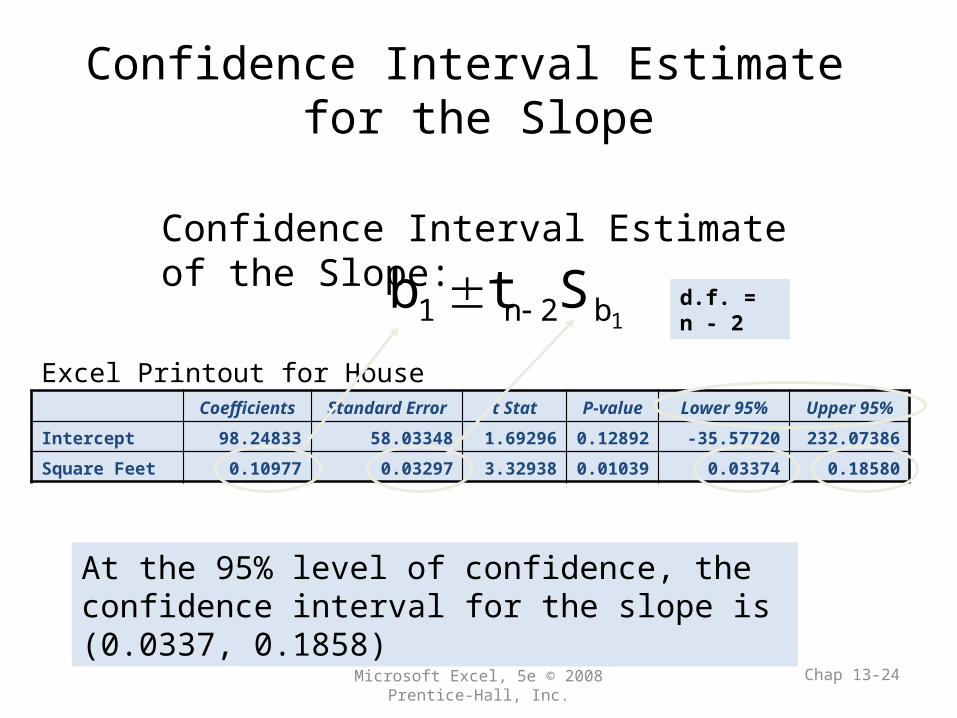
Confidence Interval Estimate for the Slope
Confidence Interval Estimate of the Slope:
Excel Printout for House Prices:
At the 95% level of confidence, the confidence interval for the slope is (0.0337, 0.1858)
1b2n1 Stb
Coefficients Standard Error t Stat P-value Lower 95% Upper 95%
Intercept 98.24833 58.03348 1.69296 0.12892 -35.57720 232.07386
Square Feet 0.10977 0.03297 3.32938 0.01039 0.03374 0.18580
d.f. = n - 2
Statistics for Managers Using Microsoft Excel, 5e © 2008 Prentice-Hall, Inc. Chap 13-25
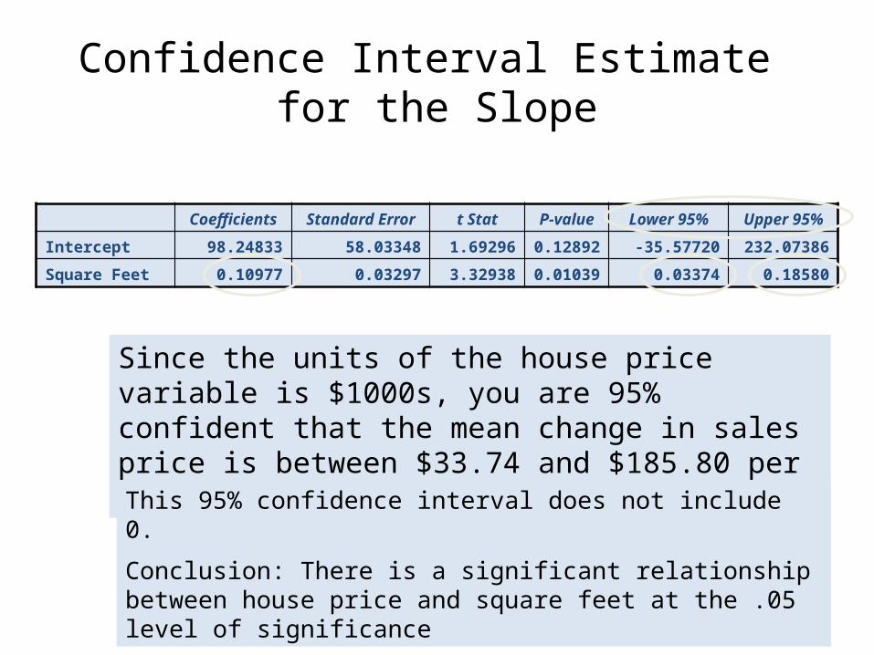
Confidence Interval Estimate for the Slope
Since the units of the house price variable is $1000s, you are 95% confident that the mean change in sales price is between $33.74 and $185.80 per square foot of house size
Coefficients Standard Error t Stat P-value Lower 95% Upper 95%
Intercept 98.24833 58.03348 1.69296 0.12892 -35.57720 232.07386
Square Feet 0.10977 0.03297 3.32938 0.01039 0.03374 0.18580
This 95% confidence interval does not include 0.
Conclusion: There is a significant relationship between house price and square feet at the .05 level of significance
Statistics for Managers Using Microsoft Excel, 5e © 2008 Prentice-Hall, Inc. Chap 13-26
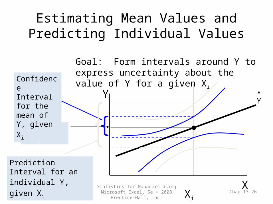
Estimating Mean Values and Predicting Individual Values
X
Y = b0+b1Xi
Confidence Interval for the mean of
Y, given Xi
Prediction Interval for an
individual Y, given Xi
Goal: Form intervals around Y to express uncertainty about the value of Y for a given Xi
Y
Xi
Y
Statistics for Managers Using Microsoft Excel, 5e © 2008 Prentice-Hall, Inc. Chap 13-27
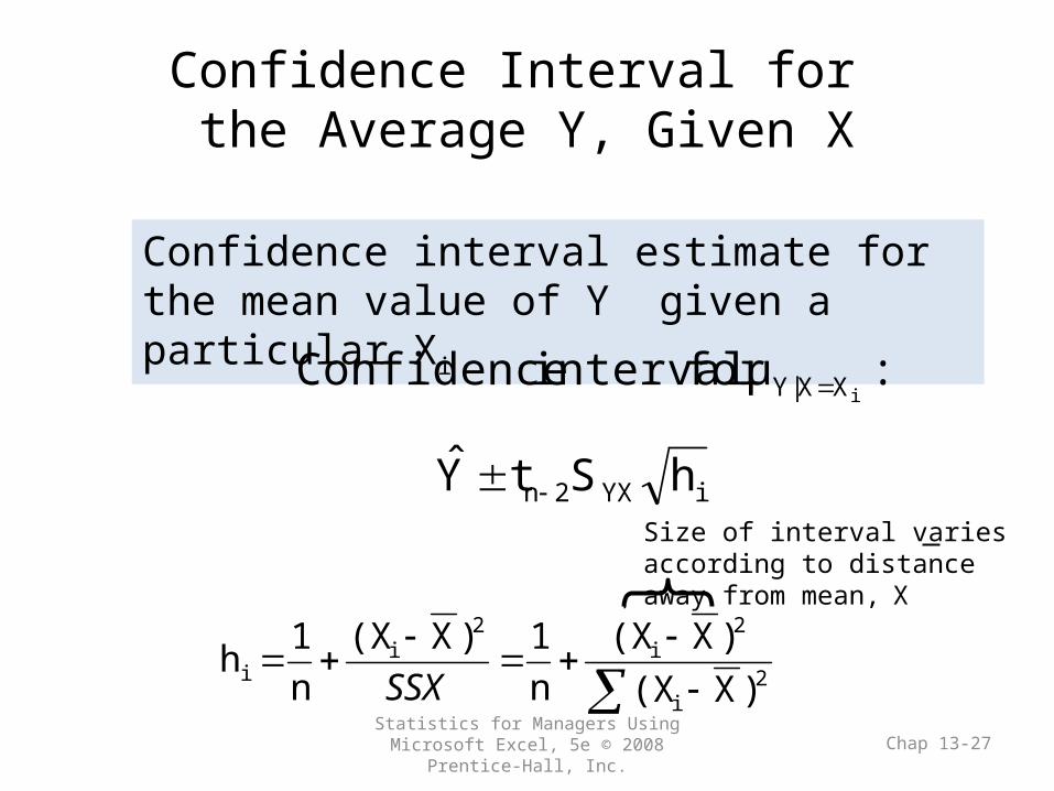
Confidence Interval for the Average Y, Given X
Confidence interval estimate for the mean value of Y given a particular Xi
Size of interval varies according to distance away from mean, X
iYX2n
XX|Y
hStY
:μ for interval Confidencei
2
i
2i
2i
i)X(X
)X(X
n
1)X(X
n
1h
SSX
Statistics for Managers Using Microsoft Excel, 5e © 2008 Prentice-Hall, Inc. Chap 13-28
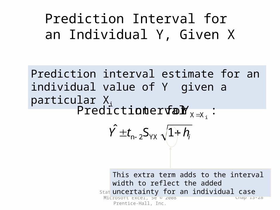
Prediction Interval for an Individual Y, Given X
Prediction interval estimate for an individual value of Y given a particular Xi
This extra term adds to the interval width to reflect the added uncertainty for an individual case
ihtY
1Sˆ
:Yfor interval Prediction
YX2n
XX i
Statistics for Managers Using Microsoft Excel, 5e © 2008 Prentice-Hall, Inc. Chap 13-29
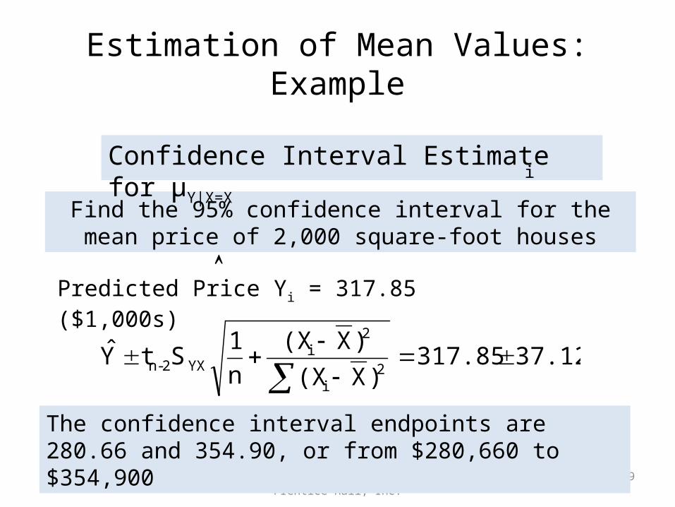
Estimation of Mean Values: Example
Find the 95% confidence interval for the mean price of 2,000 square-foot houses
Predicted Price Yi = 317.85 ($1,000s)
Confidence Interval Estimate for μY|X=X
37.12317.85)X(X
)X(X
n
1StY
2i
2i
YX2-n
The confidence interval endpoints are 280.66 and 354.90, or from $280,660 to $354,900
i

Statistics for Managers Using Microsoft Excel, 5e © 2008 Prentice-Hall, Inc. Chap 13-30
Estimation of Individual Values: Example
Find the 95% prediction interval for an individual house with 2,000 square feet
Predicted Price Yi = 317.85 ($1,000s)
Prediction Interval Estimate for YX=X
102.28317.85)X(X
)X(X
n
11StY
2i
2i
YX1-n
The prediction interval endpoints are 215.50 and 420.07, or from $215,500 to $420,070
i

• Hypotheses – H0: ρ = 0 (no correlation between X and Y)
– H1: ρ ≠ 0 (correlation exists)
• Test statistic (with n – 2 degrees of
freedom)
Statistics for Managers Using Microsoft Excel, 5e © 2008 Prentice-Hall, Inc. Chap 13-31
t Test for a Correlation Coefficient
2nr1
ρ-rt
2
0 b if rr
0 b if rr
where
12
12
Statistics for Managers Using Microsoft Excel, 5e © 2008 Prentice-Hall, Inc. Chap 13-32
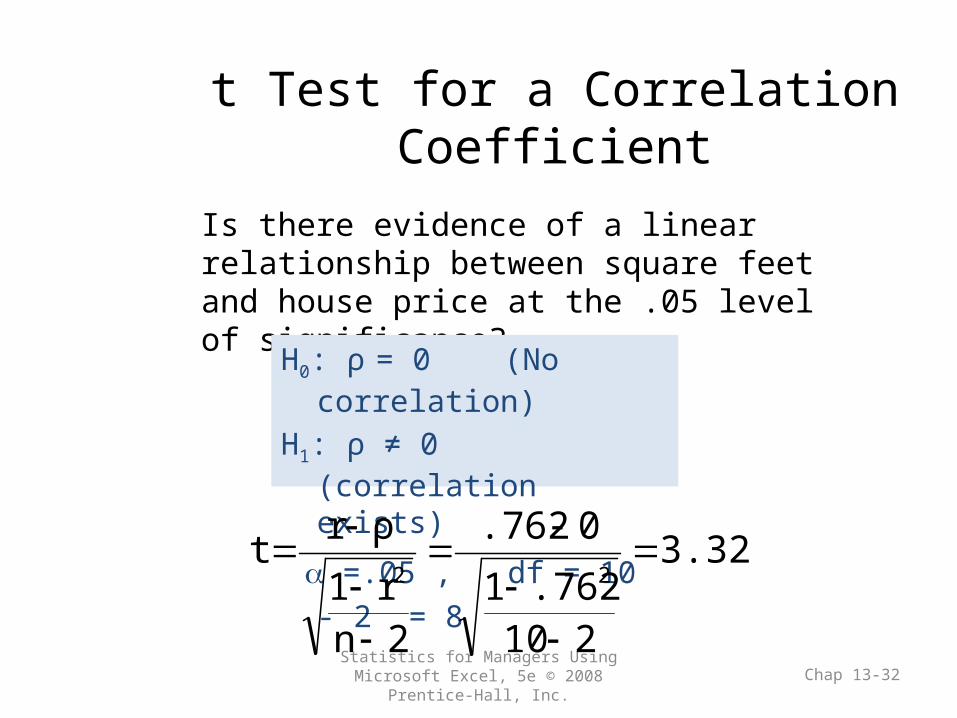
t Test for a Correlation Coefficient
Is there evidence of a linear relationship between square feet and house price at the .05 level of significance?
H0: ρ = 0 (No correlation)
H1: ρ ≠ 0 (correlation exists)
=.05 , df = 10 - 2 = 8
3.329
210.7621
0.762
2nr1
ρrt
22
Statistics for Managers Using Microsoft Excel, 5e © 2008 Prentice-Hall, Inc. Chap 13-33
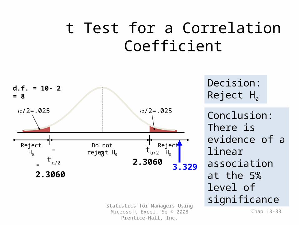
t Test for a Correlation Coefficient
Reject H0Reject H0
a/2=.025
-tα/2Do not reject H0
0 tα/2
a/2=.025
-2.3060 2.3060 3.329
d.f. = 10- 2 = 8
Conclusion:There is evidence of a linear association at the 5% level of significance
Decision:Reject H0

Statistics for Managers Using Microsoft Excel, 5e © 2008 Prentice-Hall, Inc. Chap 13-34
Residual Analysis
• The residual for observation i, ei, is the difference between its observed and predicted value
• Check the assumptions of regression by examining the residuals– Examine for Linearity assumption– Evaluate Independence assumption – Evaluate Normal distribution assumption– Examine Equal variance for all levels of X
• Graphical Analysis of Residuals– Can plot residuals vs. X
iii YYe ˆ

Statistics for Managers Using Microsoft Excel, 5e © 2008 Prentice-Hall, Inc. Chap 13-35
Residual Analysis for Linearity
Not Linear Linear
x
resi
dual
s
x
Y
x
Y
x
resi
dual
s

Statistics for Managers Using Microsoft Excel, 5e © 2008 Prentice-Hall, Inc. Chap 13-36
Residual Analysis for Independence
Not Independent Independent
X
Xresi
dual
s
resi
dual
s
X
resi
dual
s

Statistics for Managers Using Microsoft Excel, 5e © 2008 Prentice-Hall, Inc. Chap 13-37
Checking for Normality
• Examine the Stem-and-Leaf Display of the Residuals
• Examine the Box-and-Whisker Plot of the Residuals
• Examine the Histogram of the Residuals• Construct a Normal Probability Plot of
the Residuals
Statistics for Managers Using Microsoft Excel, 5e © 2008 Prentice-Hall, Inc. Chap 13-38
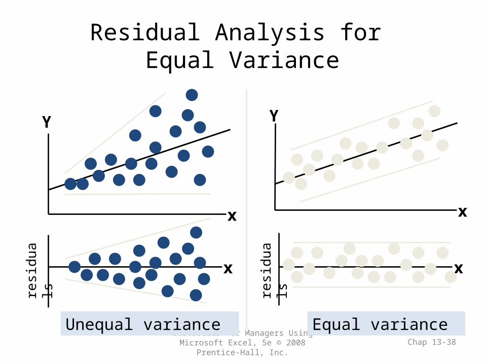
Residual Analysis for Equal Variance
Unequal variance Equal variance
x x
Y
x x
Y
resi
dual
s
resi
dual
s
Statistics for Managers Using Microsoft Excel, 5e © 2008 Prentice-Hall, Inc. Chap 13-39
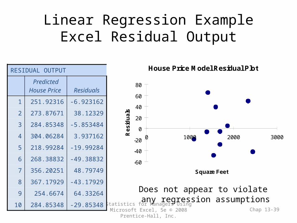
Linear Regression ExampleExcel Residual Output
House Price Model Residual Plot
-60
-40
-20
0
20
40
60
80
0 1000 2000 3000
Square Feet
Re
sid
ua
ls
RESIDUAL OUTPUT
Predicted House Price Residuals
1 251.92316 -6.923162
2 273.87671 38.12329
3 284.85348 -5.853484
4 304.06284 3.937162
5 218.99284 -19.99284
6 268.38832 -49.38832
7 356.20251 48.79749
8 367.17929 -43.17929
9 254.6674 64.33264
10 284.85348 -29.85348Does not appear to violate any regression assumptions
Statistics for Managers Using Microsoft Excel, 5e © 2008 Prentice-Hall, Inc. Chap 13-40
Measuring Autocorrelation:The Durbin-Watson Statistic
• Used when data are collected over time to detect if autocorrelation is present
• Autocorrelation exists if residuals in one time period are related to residuals in another period

Statistics for Managers Using Microsoft Excel, 5e © 2008 Prentice-Hall, Inc. Chap 13-41
Autocorrelation
• Autocorrelation is correlation of the errors (residuals) over time
Violates the regression assumption that residuals are statistically independent
Time (t) Residual Plot
-15
-10
-5
0
5
10
15
0 2 4 6 8
Time (t)
Res
idu
als Here, residuals suggest a
cyclic pattern, not random
Statistics for Managers Using Microsoft Excel, 5e © 2008 Prentice-Hall, Inc. Chap 13-42
Strategies for Avoiding the Pitfalls of Regression
• Start with a scatter plot of X on Y to observe possible relationship
• Perform residual analysis to check the assumptions– Plot the residuals vs. X to check for violations of
assumptions such as equal variance– Use a histogram, stem-and-leaf display, box-and-
whisker plot, or normal probability plot of the residuals to uncover possible non-normality

Statistics for Managers Using Microsoft Excel, 5e © 2008 Prentice-Hall, Inc. Chap 13-43
Strategies for Avoiding the Pitfalls of Regression
• If there is violation of any assumption, use alternative methods or models
• If there is no evidence of assumption violation, then test for the significance of the regression coefficients and construct confidence intervals and prediction intervals
• Avoid making predictions or forecasts outside the relevant range