Linear Regression and Regression Trees Avinash Kak Purdue ... · The Regression Tree Tutorial by...

Linear Regression and Regression Trees

Avinash Kak

Purdue University

April 28, 2019

4:04pm

An RVL Tutorial Presentation

Originally presented on April 29, 2016

Minor edits made in April 2019

c©2019 Avinash Kak, Purdue University

The Regression Tree Tutorial by Avi Kak

CONTENTS

Page

1 Regression In General 3

2 Introduction to Linear Regression 6

3 Linear Regression Through 9Equations

4 A Compact Representation for 15All Observed Data

5 Estimating the p+1 Regression 18Coefficients

6 Refining the Estimates for the 23Regression Coefficients

7 Regression Trees 39

8 The RegressionTree Class in My 41Python and Perl DecisionTreeModules

9 API of the RegressionTree Class 53

10 The ExamplesRegression Directory 60

11 Acknowledgment 63

2


1. Regression In General

• Regression, in general, helps us understand

relationships between variables that are not

amenable to analysis through causal phe-

nomena. This is the case with many vari-

ables about us as human beings and about

many socioeconomic aspects of our soci-

eties.

• As a case in point, we know intuitively that

our heights and weights are correlated —

in the colloquial sense that the taller one

becomes, the more likely that one’s weight

will go up. [If we were to sample, say, 1000 individuals

and make a plot of the height versus weight values, we are

likely to see a scatter plot in which for each height you will

see several different weights. But, overall, the scatter plot will

show a trend indicating that, on the average, we can expect

the weight to go up with the height.]

3


• Central to the language of regression are

the notions of one designated dependent

variable and one or more predictor vari-

ables. In the height-vs.-weight example,

we can think of the weight as the depen-

dent variable and the height as the predic-

tor variable. For that example, the goal

of a regression algorithm would be to re-

turn the best (best in some average sense)

value for the weight for a given height.

• Of all the different regression algorithms —

and there are virtually hundreds of them

out there now — linear regression is ar-

guably the most commonly used. What

adds to the “versatility” of linear regres-

sion is the fact that it includes polynomial

regression in which you are allowed to use

powers of the predictor variables for esti-

mating the likely values for the dependent

variable.

4


• While linear regression has sufficed for many

applications, there are many others where

it fails to perform adequately. Just to il-

lustrate this point with a simple example,

shown below is some noisy data for which

linear regression yields the line shown in

red.

• The blue line is the output of the tree re-

gression algorithm that is presented in the

second half of this tutorial.

5


2. Introduction to Linear Regression

• The goal of linear regression is to make

a “best” possible estimate of the general

trend regarding the relationship between

the predictor variables and the dependent

variable with the help of a curve that most

commonly is a straight line, but that is al-

lowed to be a polynomial also.

• The fact that the relationship between the

predictor variables and the dependent vari-

able can be nonlinear adds to the power

of linear regression — for obvious reasons.

[As to why the name of the algorithm has “Linear” in it con-

sidering that it allows for polynomial relationships between

the predictor and the dependent variables, the linearity in the

name refers to the relationship between the dependent vari-

able and the regression coefficients.]

6


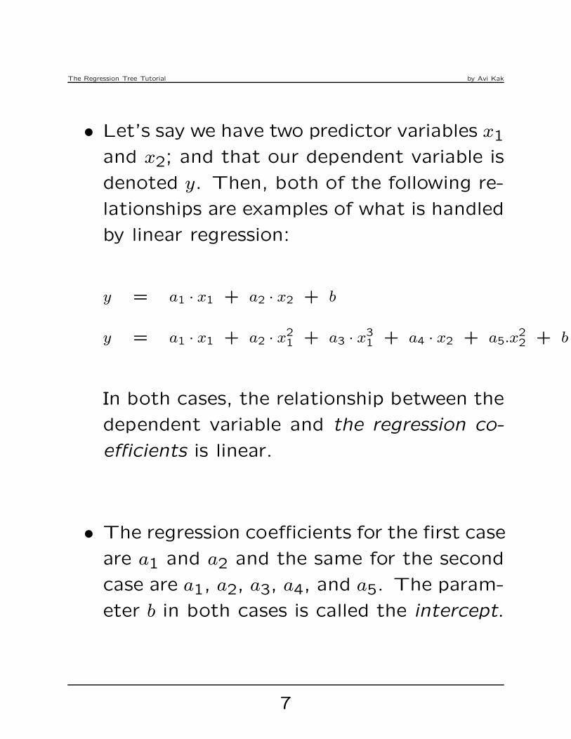
• Let’s say we have two predictor variables x1

and x2; and that our dependent variable is

denoted y. Then, both of the following re-

lationships are examples of what is handled

by linear regression:

y = a1 · x1 + a2 · x2 + b

y = a1 · x1 + a2 · x21 + a3 · x3

1 + a4 · x2 + a5.x22 + b

In both cases, the relationship between the

dependent variable and the regression co-

efficients is linear.

• The regression coefficients for the first case

are a1 and a2 and the same for the second

case are a1, a2, a3, a4, and a5. The param-

eter b in both cases is called the intercept.

7


• The fact that linear regression allows for

the powers of the predictor variables to

appear in the relationship between the de-

pendent and the predictor variables is com-

monly referred to by saying that it includes

polynomial regression.

8


3. Linear Regression Through Equations

• In this tutorial, we will always use y to rep-

resent the dependent variable. A depen-

dent variable is the same thing as the pre-

dicted variable. And we use the vector ~x

to represent a p-dimensional predictor.

• In other words, we have p predictor vari-

ables, each corresponding to a different di-

mension of ~x.

• Linear regression is based on assuming that

the relationship between the dependent and

the predictor variables can be expressed as:

y = ~xT ~β + b (1)

9


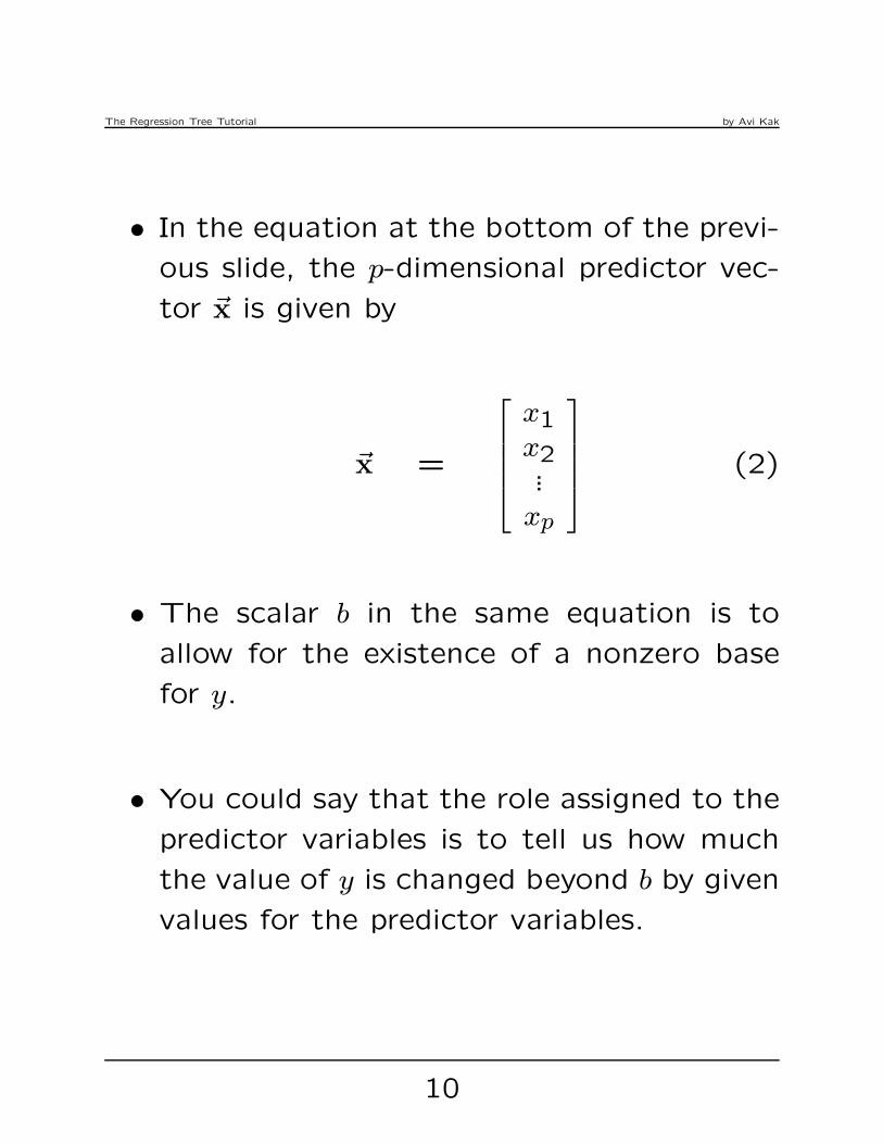
• In the equation at the bottom of the previ-

ous slide, the p-dimensional predictor vec-

tor ~x is given by

~x =

x1x2...xp

(2)

• The scalar b in the same equation is to

allow for the existence of a nonzero base

for y.

• You could say that the role assigned to the

predictor variables is to tell us how much

the value of y is changed beyond b by given

values for the predictor variables.

10


• In Eq. (1), the vector ~β consists of p co-

efficients as shown below:

~β =

β1β2...βp

(3)

that reflect the weights to be given to the

different predictor variables in ~x with regard

to their predictive power.

• The very first thought that pops up in one’s

head when one looks at Eq. (1) is that the

scalar y depends linearly on the predictor

variables {x1, x2, · · · , xp}. It is NOT this

linearity that the linear regression refers to

through its name. As mentioned earlier,

the predictor variables are allowed to be

powers of what it is that is doing the pre-

diction.

11


• Let’s say that in reality we have only two

predictor variables x1 and x2 and that the

relationship between y and these two pre-

dictors is given be y = β1x1+β2x2+β3x21+

β4x31 + b where we have now included the

second and the third powers of the vari-

able x1. For linear regression based com-

putations, we express such a relationship

as y = β1x1+β2x2+β3x3+β4x4+ b where

x3 = x21 and x4 = x31. The linearity that

linear regression refers to is related to lin-

earity with respect to the regression coef-

ficients {β1, β2, · · · , βp, b}.

• For the reasons state above, linear regres-

sion includes polynomial regression in which

the prediction is made from the actual pre-

dictor variables and their various powers.

12


• For a more efficient notation and for posi-

tioning ourselves for certain algebraic ma-

nipulations later on, instead of using pre-

dictor vector ~x as shown in Eq. (2), we

will use its augmented form shown below:

~x =

x1x2...xp1

(4)

• Additionally, we will now denote the base-

value scalar b by the notation:

βp+1 = b (5)

• Denoting b in this manner will allow us to

make b a part of the vector of regression

coefficients as shown on the next slide.

13


• The notation ~β will now stand for:

~β =

β1β2...βpb

(6)

• Using the forms in Eqs. (4) and (6), the re-

lationship in Eq. (1) can now be expressed

more compactly as

y = ~xT ~β (7)

When using this more compact representa-

tion of the relationship between the depen-

dent variable and the predictor variables,

we must not forget that the last element

of the ~x is set to 1 and the last element of

the coefficient vector ~β is supposed to be

the base value b.

14


4. A Compact Representation for All

Observed Data

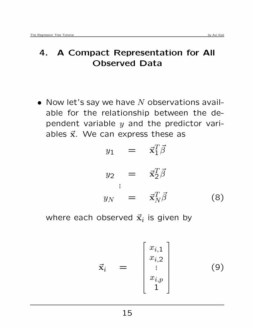
• Now let’s say we have N observations avail-

able for the relationship between the de-

pendent variable y and the predictor vari-

ables ~x. We can express these as

y1 = ~xT1~β

y2 = ~xT2~β

...

yN = ~xTN~β (8)

where each observed ~xi is given by

~xi =

xi,1xi,2...

xi,p1

(9)

15


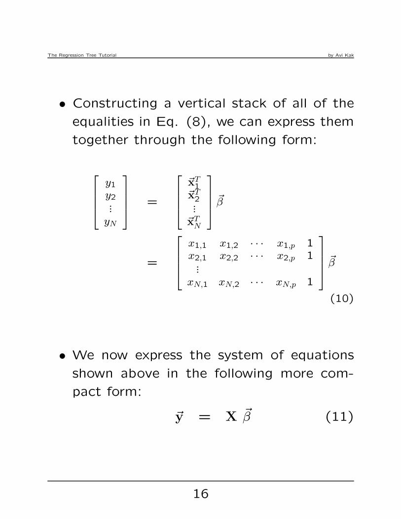
• Constructing a vertical stack of all of the

equalities in Eq. (8), we can express them

together through the following form:

y1y2...yN

=

~xT1

~xT2...

~xTN

~β

=

x1,1 x1,2 · · · x1,p 1x2,1 x2,2 · · · x2,p 1...

xN,1 xN,2 · · · xN,p 1

~β

(10)

• We now express the system of equations

shown above in the following more com-

pact form:

~y = X ~β (11)

16


• In the last equation on the previous slide,

the N × p matrix X is given by

X =

x1,1 x1,2 · · · x1,p 1

x2,1 x2,2 · · · x2,p 1...

xN,1 xN,2 · · · xN,p 1

(12)

• The matrix X is sometimes called the “de-

sign matrix”. Note that, apart from the

number 1 for its last element, each row of

the design matrix X corresponds to one

observation for all p predictor variables. In

total, we have N observations.

• The goal of linear regression is to esti-

mate the p+1 regression coefficients in

the vector ~β from the system of equa-

tions in Eq. (11). Recall the form of the~β vector as provided in Eq. (6).

17


5. Estimating the p+1 Regression

Coefficients

• To account for noise in the measurement

of the dependent variable y (and assuming

that the values for the predictor variables

are known exactly for each of the N obser-

vations), we may prefer to write Eq. (11)

as

~y = X ~β + ~ǫ (13)

• Assuming that N > p+1 and that the dif-

ferent observations for the dependent vari-

able are more or less independent, the rank

of X is p+1. Our goal now is to estimate

the p + 1 dimensional vector ~β from the

overdetermined system of equations through

the minimization of the cost function

C(~β) = ‖~y − X ~β‖2 (14)

18


• Ignoring for now the error term ~ǫ in Eq.

(13), note that what we are solving is an

inhomogeneous system of equations given

by ~y = X ~β. This system of equations is

inhomogeneous since the vector ~y cannot

be all zeros.

• The optimum solution for ~β that minimizes

the cost function C(~β) in Eq. (14) pos-

sesses the following geometrical interpre-

tation: Focusing on the equation ~y = X~β, the measured

vector ~y on the left resides in a large N dimensional space.

On the other hand, as we vary ~β in our search for the best

possible solution, the space spanned by the product X~β will

be a (p+1)-dimensional subspace (a hyperplane, really) in the

N dimensional space in which ~y resides. The question now

is: which point in the hyperplane spanned by X~β is the best

approximation to the point ~y which is outside the hyperplane.

For any selected value for ~β, the “error” vector ~y − X~β will

go from the tip of the vector X~β to the tip of the ~y vector.

Minimization of the cost function C in Eq. (14) amounts to

minimizing the norm of this difference vector.

19


• The norm in question is minimized when

we choose for ~β a vector so that X~β is

the perpendicular projection of ~y into the

(p + 1)-dimensional row space of the ma-

trix X. The difference vector ~y − X~β at

the point in the row space of X where this

perpendicular projection of ~y falls satisfies

the following constraint:

XT · (~y − X ~β) = 0 (15)

• This implies the following solution for ~β:

~β = (XTX)−1XT~y (16)

• If we denote the pseudoinverse of X by X+,

we can write for the solution:

~β = X+~y (17)

where the pseudoinverse is given by X+ = (XTX)−1XT .

20


• Note that XTX is a square (p+1)×(p+1)

matrix whose rank is exactly p+1. That is

a consequence of the fact that rank(X) =

p+1. XTX being of full rank implies that

the inverse (XTX)−1 is guaranteed to exist.

• In general, for real valued matrices, XTX

will always be symmetric and positive semidef-

inite. The eigenvalues for a such a product

matrix will always be real and nonnegative.

• At this point, it is good to reflect on the

composition of the matrix X shown in Eq.

(12). Each row of X consists of one ob-

servation for all the p predictor variables

following by the number 1.

21


• We say that the solution shown in Eq. (16)

is a a result of linear least squares mini-

mization from a system of inhomogeneous

equations. The characterization “linear” in

“linear least squares minimization” refers

to the fact that we developed our solution

from a system of linear equations.

22


6. Refining the Estimates for the

Regression Coefficients

• The solution that is obtained with linear

least-squares minimization can be further

refined with nonlinear least-squares min-

imization.

• An informed reader would say: Where

is the need for such refinement? Such

a reader would go on to say that since

the linear least-squares estimate for the re-

gression coefficients in the previous section

was obtained by minimizing a convex cost

function (implying that this function has a

unique global minimum and no other local

minima), we can be reasonably certain that

the minimum yielded by the solution in the

previous section is as good as it can get.

23


• Nonetheless, in order to allow for the fact

that real data can be complex and a linear

regression model is at best an approxima-

tion to whatever true relationship there ex-

ists between the predictor variables and the

dependent variable, I am going to go ahead

and develop a nonlinear least-squares based

estimation refinement method in this sec-

tion.

• Before going ahead, though, I wish to say

at the very outset that for all the synthetic

examples I will be presenting in a later sec-

tion, you do not need any refinement at

all. If you do try to refine them with the formulas

shown in this section, yes, you do get an answer

that looks slightly different (in some cases, per-

haps visually more appropriate) — but with an MSE

(mean-squared error) that is very slightly greater

than what you get with just plain least-squares. I

attribute this increase in MSE to issues related

to how you terminate a gradient-descent path

to the minimum.

24


• With all the caveats out of the way, let me

now focus on how we may go about “refin-

ing” the estimates of the previous section.

• With nonlinear least-squares minimization,

we now think of a cost function in the

space spanned by the the p + 1 elements

of the ~β vector. (Recall, in linear least-

squares minimization, we were focused on

how to best project the N-dimensional mea-

surement vector ~y into the (p+1)-dimensional

space spanned by the row vectors of the

matrix X.)

• Think now of the hyperplane as spanned

by the elements of ~β and a cost function

C(~β) as the height of a surface above the

hyperplane.

25


• Our goal is find that point in the hyper-

plane where the height of the surface is the

least. In other words, our goal is the find

that point ~β that gives us the global min-

imum for the height of the surface. Such

a global minimum is generally found by an

iterative algorithm that starts somewhere

in the hyperplane, looks straight up at the

surface, and then takes small incremental

steps along those directions in the hyper-

plane that yield descents on the surface to-

wards the global minimum. This, as you

surely know already, is the essence of the

gradient descent algorithms.

• In general, though, the surface above the

hyperplane may possess both a global mini-

mum and an arbitrary number of local min-

ima. (Cost functions must be convex for

there to exist just a single global minimum.

In our case, there is no guarantee that C(~β)

is convex.)

26


• Considering that, in general, a cost func-

tion surface may possess local minima, our

only hope is to start the search for the

global minimum from somewhere that is

in its vicinity. The consequences of start-

ing the search from an arbitrary point in

the hyperplane are obvious — we could get

trapped in a local minimum.

• Experience has shown that if we start the

search at that point in the hyperplane spanned

the unknown vector ~β that corresponds to

somewhere in the vicinity of the linear least-

squares solution, we are likely to not get

trapped in a local minimum. If ~β0 denotes

this point in the hyperplane, we set

~β0 = α · (XTX)−1XT~y (18)

for some value of the multiplier α between

0 and 1.

27


• Subsequently, in the gradient descent ap-

proach, we calculate the next point in the

hyperplane through the following calcula-

tion:

~βk+1 = ~βk − γ · ∇C∣

∣

∣~β=~βk(19)

where γ is called the step size controller

and ∇C is the gradient of the surface at

point ~β = ~βk in the supporting hyperplane

for the cost function surface.

• We stop the iterations either after a certain

fixed number of them or when the step size

‖~βk+1 − ~βk‖ falls below some threshold.

• Before the iterative formula dictated by Eq.

(19) can be used, the issue of how to com-

pute the gradient ∇C(~β) remains.

28


• In order to compute this gradient, we ex-

press our cost function C(~β) in the follow-

ing form:

C(~β) = ‖~y − ~g(~β)‖2 (20)

where ~g(~β) is a function that relates the

parameters to be estimated, ~β, and the ac-

tual measurements ~y. For the linear least-

squares solution in the previous section,

we assumed that ~g(~β) = X · ~β. But now

we want to allow for the possibility that

while, nominally, the relationship between

the measurements ~y and ~β is linear, ac-

tual data may demand nonlinear degrees

of freedom with regard to how the param-

eters ~β relate to the measurements. [The

parameter βi reflects the weight to be given to the

predictor xi for making a y prediction. What if this

weight does not remain exactly the same over the

entire scale over which xi can vary?]

29


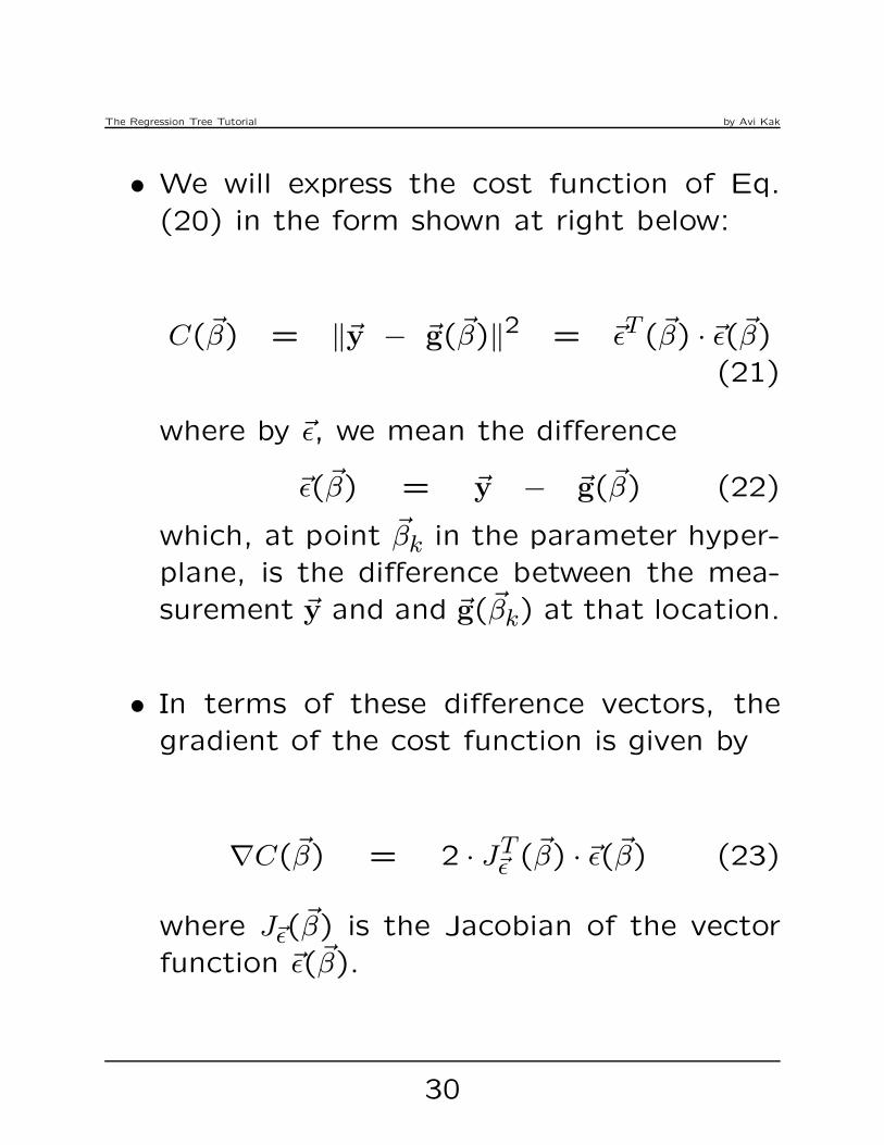
• We will express the cost function of Eq.

(20) in the form shown at right below:

C(~β) = ‖~y − ~g(~β)‖2 = ~ǫT (~β) · ~ǫ(~β)

(21)

where by ~ǫ, we mean the difference

~ǫ(~β) = ~y − ~g(~β) (22)

which, at point ~βk in the parameter hyper-

plane, is the difference between the mea-

surement ~y and and ~g(~βk) at that location.

• In terms of these difference vectors, the

gradient of the cost function is given by

∇C(~β) = 2 · JT~ǫ (~β) · ~ǫ(~β) (23)

where J~ǫ(~β) is the Jacobian of the vector

function ~ǫ(~β).

30


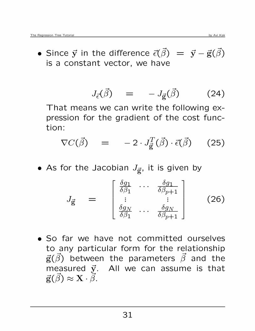
• Since ~y in the difference ~ǫ(~β) = ~y − ~g(~β)is a constant vector, we have

J~ǫ(~β) = − J~g(

~β) (24)

That means we can write the following ex-pression for the gradient of the cost func-tion:

∇C(~β) = − 2 · JT~g (~β) · ~ǫ(~β) (25)

• As for the Jacobian J~g, it is given by

J~g =

δg1δβ1

· · · δg1δβp+1

... ...δgNδβ1

· · · δgNδβp+1

(26)

• So far we have not committed ourselvesto any particular form for the relationship~g(~β) between the parameters ~β and themeasured ~y. All we can assume is that~g(~β) ≈ X · ~β.

31


• Keeping in mind the approximation shown

in the previous bullet, one can argue that

we may approximate the Jacobian shown in

Eq. (26) by first calculating the difference

between the vectors X·(~β+δ~β) and X~β, di-

viding each element of the difference vector

by the β increment, and finally distributing

the elements of the vector thus obtained

according to the matrix shown in Eq. (26).

[We will refer to this as the “jacobian choice=2” op-

tion in the next section.]

• As a counterpoint to the arguments made

so far for specifying the Jacobian, it is in-

teresting to think that if one yielded to the

temptation of creating an analytical form

for the Jacobian using the ~y = X · ~β rela-

tionship, one would end up (at least the-

oretically) with the same solution as the

linear least-squares solution of Eq. (17).

A brief derivation on the next slide establishes this

point.

32


• From the first element of the first row of

the matrix in Eq. (26), we know from Eq.

(10) that

(X~β)i = xi,1β1+· · ·+xi,pβp+βp+1 i = 1, · · · , N(27)

Therefore,

δ(X~β)i

δβj

= xi,j i = 1, · · · , N and j = 1, · · · , p

δ(X~β)i

δβp+1

= 1 i = 1, · · · , N (28)

• Substituting these partial derivatives in Eq.

(26), we can write for the N × (p+1) Ja-

cobian:

JX~β

=

x1,1 · · · x1,p 1... ...

xN,1 · · · xN,p 1

= X

(29)

33


• Substituting this result in Eq. (25), we can

write for the gradient of the cost function

surface at a point ~β in the ~β-hyperplane:

∇C(~β) = − 2 ·XT · ~ǫ(~β) (30)

• The goal of a gradient-descent algorithm

is to find that point in the space spanned

by the p+1 dimensional β vector where the

gradient given by Eq. (30) is zero. When

you set this gradient to zero while using

~ǫ(~β) = ~y −X · ~β, you get exactly the same

solution as given by Eq. (17).

• Despite the conclusion drawn above, it’s

interesting nonetheless to experiment with

the refinement formulas when the Jaco-

bian is to the matrix X as dictated by Eq.

(29). [We will refer to this as the option

“jacobian choice=1” in the next section.]

34


• Shown below is a summary of the Gradi-

ent Descent Algorithm for refining the es-

timate produced by the linear least-squares

algorithm of the previous section.

Step 1: Given the N observations of the de-

pendent variable, while knowing at the same

time the corresponding p predictor variables,

we set up an algebraic system of equations

as shown in Eq. (8). Note that in these

equations, we have already augmented the

predictor vector ~x by the number 1 for its

last element and the ~β vector by the inter-

cept b (as argued in Section 3).

Step 2: We stack all the equations together

into the form shown in Eq. (11) and (12):

~y = X ~β (31)

35


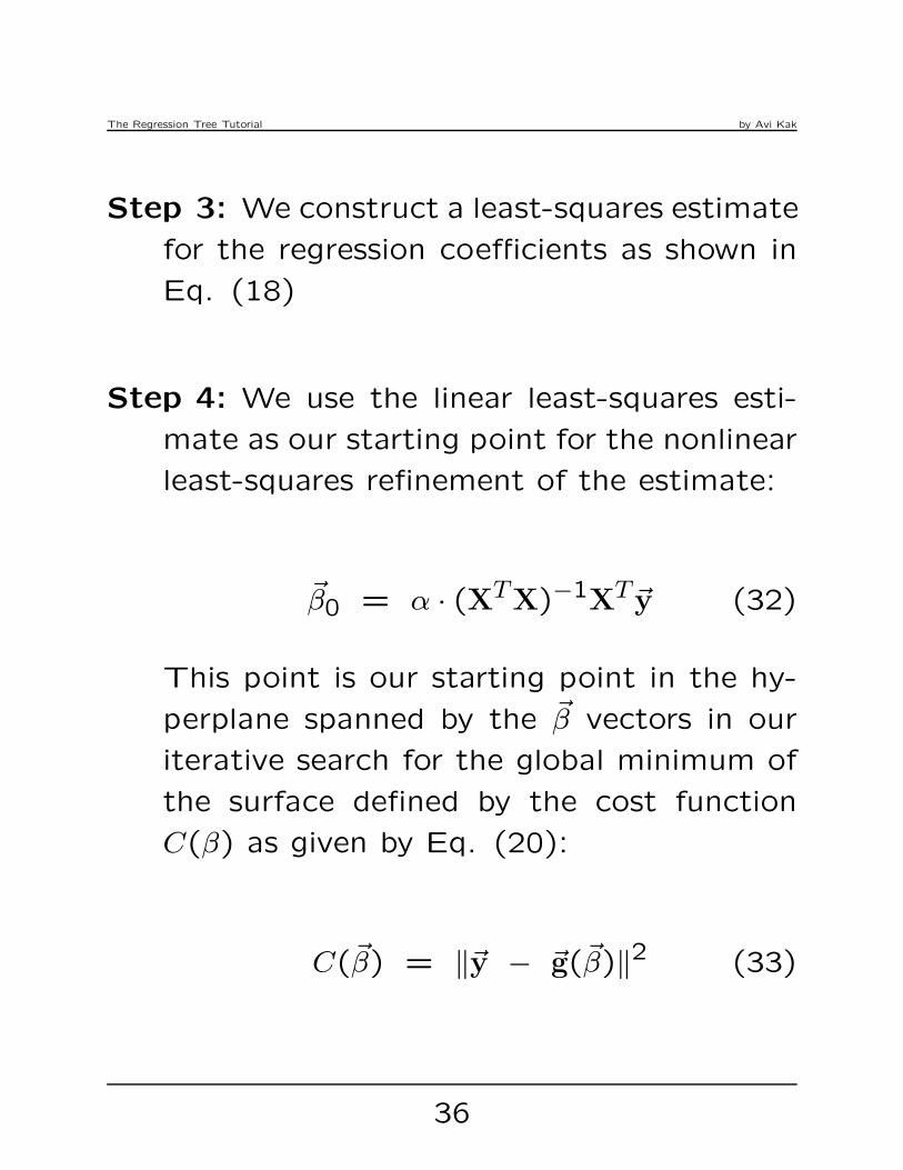
Step 3: We construct a least-squares estimate

for the regression coefficients as shown in

Eq. (18)

Step 4: We use the linear least-squares esti-

mate as our starting point for the nonlinear

least-squares refinement of the estimate:

~β0 = α · (XTX)−1XT~y (32)

This point is our starting point in the hy-

perplane spanned by the ~β vectors in our

iterative search for the global minimum of

the surface defined by the cost function

C(β) as given by Eq. (20):

C(~β) = ‖~y − ~g(~β)‖2 (33)

36


Step 5: We next estimate the Jacobian at the

current solution point by using the matrix

in Eq. (26).

Step 6: We now carry out the iterative march

toward the global minimum using the for-

mulas shown in Eqs. (19) and (25):

~βk+1 = ~βk + γ ·JT~g (~β) ·(~y−X~β) (34)

where we use for the Jacobian either of the

two options “jacobian choice=1” or “jacobian choice=2”

described earlier in this section. To these

two options, we will add the “jacobian choice=0”

option to indicate the case when we do not

want any refinement.

37


Step 7: We stop the iterations either after a

prespecified number of them have been ex-

ecuted or when the step size ‖~βk+1 − ~βk‖

falls below a prespecified threshold.

38


7. Regression Trees

• You can think of regression with a regres-

sion tree as a powerful generalization of

the linear regression algorithm we have pre-

sented so far in this tutorial.

• Although you can certainly carry out poly-

nomial regression with run-of-the-mill lin-

ear regression algorithms for modeling non-

linearities between the predictor variables

and the dependent variable, specifying the

degree of the polynomial is often a tricky

business.

• Additionally, a polynomial can inject conti-

nuities between the predictor and the pre-

dicted variables that may not actually exist

in the real data.

39


• Regression trees, on the other hand, give

you a piecewise linear relationship between

the predictor and the predicted variables

that is freed from the constraints of super-

imposed continuities at the joins between

the different segments.

40


8. The RegressionTree Class in My

Python and Perl DecisionTree Modules

• The rest of this tutorial is about the RegressionTree

class that is a part of my Python and Perl

DecisionTree modules. More precisely speak-

ing, RegressionTree is a subclass of the main

DecisionTree class in both cases. Here are

the links to the download pages for the

DecisionTree modules:

https://pypi.python.org/pypi/DecisionTree/3.4.3

http://search.cpan.org/~avikak/Algorithm-DecisionTree-3.43/lib/Algorithm/DecisionTree.pm

Just clicking on the links should take you

directly to the relevant webpages at the

Python and Perl repositories from where

you can get access to the module files.

41

https://pypi.python.org/pypi/DecisionTree/3.4.3

http://search.cpan.org/~avikak/Algorithm-DecisionTree-3.43/lib/Algorithm/DecisionTree.pm


• By making RegressionTree a subclass of

DecisionTree, the former is able to call upon

the latter’s functionality for computations

needed for growing a tree. [These compu-

tations refer to keeping track of the feature names

and their associated values, figuring the data sam-

ples relevant to a node in the tree taking into ac-

count the threshold inequalities on the branches

from the root to the node, etc.]

• The current version of the RegressionTree class

can only deal with purely numerical data.

This is unlike what the DecisionTree module

is capable of. The DecisionTree module al-

lows for arbitrary mixtures of symbolic and

numerical features in your training dataset.

• My goal is that a future version of RegressionTree

will call upon some of the additional func-

tionality already built into the DecisionTree

class to allow for a mixture of symbolic and

numerical features to be used for creating

a predictor for numeric variable.

42


• The basic idea involved in using formulas

derived in the previous section in order to

grow a regression tree is simple. The cal-

culations we carry out at each step are

listed in the next several bullets.

• As illustrated by the figure shown below,

you start out with all of your data at the

root node and you apply the linear regres-

sion formulas there for every bipartition of

every feature.

jθmse(f < )

jmse(f >= θ)

Feature Tested at Root

f j

• For each feature, you calculate the MSE

(Mean Squared Error) per sample for every

possible partition along the feature axis.

43


• For each possible bipartition threshold θ,

you associate it with the larger of the MSE

for the two partitions. [To be precise, this

search for the best possible partitioning point along

each feature is from the 10th point to the 90th

point in rank order of all the sampling points along

the feature axis. This is done in order to keep the

calculations numerically stable. If the number of

points retained for a partition is too few, the ma-

trices you saw earlier in the least-squares formulas

may become singular.]

• And, with each feature overall, you retain

the minimum of the MSE value calculated

in the previous step. We refer to retaining

this minimum for all threshold-based maxi-

mum values as the minmax operation applied

to a features.

• You select that feature at a node that yields

the smallest value for the MSE values as-

sociated with the feature in the previous

step.

44


• At each node below the root, you only deal

with the data samples that are relevant to

that node. You find these samples by ap-

plying the branch thresholds along the path

from the root to the node to all of the

training data.

• You use the following criteria for the ter-

mination condition in growing a tree:

– A node is not expanded into child nodes

if the minmax value at that node is less

than the user-specified mse threshold.

– If the number of data samples relevant

to a node falls below 30, you treat that

node as a leaf node.

• I’ll now show the sort of results you can

obtain with the RegressionTree class.

45


• Shown below is the result returned by thescript whose basename is regression4 in theExamplesRegression subdirectory of the DecisionTree

module. In this case, we have a single pre-dictor variable and, as you’d expect, onedependent variable. [The predictor variable is

plotted along the horizontal axis and the dependent

variable along the vertical.]

• The blue line shows the result returned bytree regression and the red line the resultof linear regression.

46


• The result shown in the previous slide was

obtained with the “jacobian choice=0” option

for the Jacobian. As the reader will re-

call from the previous section, this option

means that we did not use the refinement.

When we turn on the option “jacobian choice=1”

for refining the coefficients, we get the re-

sult shown below:

47


• And with the option “jacobian choice=2”, we

get the result shown below:

• To me, all three results shown above look

comparable. So it doesn’t look like that

we again anything by refining the regres-

sion coefficients through gradient descent.

This observation is in agreement with the

statements made at the beginning of Sec-

tion 6 of this tutorial.

48


• The next example, shown below, also in-

volves only a single predictor variable. How-

ever, in this case, we have a slightly more

complex relationship between the predic-

tor variable and the dependent variable.

Shown below is the result obtained with

the “jacobian choice=0” option.

• The red line again is the linear regression

fit to the data, and the blue line the output

of tree regression.

49


• The result shown on the previous slide was

calculated by the script whose basename is

regression5 in the ExamplesRegression directory.

• If we use the “jacobian choice=1” option for

the same data, we get the following result:

• And, shown on the next slide is the result

with the “jacobian choice=2” option.

50


• Based on the results shown in the last three

figures, we have the same overall conclu-

sion as presented earlier: the refinement

process, while altering the shape of the re-

gression function, does not play that no-

ticeable role in improving the results.

51


• Shown below is the result for the case when

we have two predictor variables. [Think of the

two variables as defining a plane and the dependent variable

as representing the height above the plane.]

• The red scatter plot shows the fit created

by linear regression. The tree based regres-

sion fits two separate planes to the data

that are shown as the blue scatter plot.

The original noisy data is shown as the

black dots.

52


9. API of the RegressionTree Class

• Here’s how you’d call the RegressionTree

constructor in Python:

import RegressionTreetraining_datafile = "gendata6.csv"rt = RegressionTree.RegressionTree(

training_datafile = training_datafile,dependent_variable_column = 3,predictor_columns = [1,2],mse_threshold = 0.01,max_depth_desired = 2,jacobian_choice = 0,

)

and here’s you would call it in Perl:

use Algorithm::RegressionTree;my $training_datafile = "gendata6.csv";my $rt = Algorithm::RegressionTree->new(

training_datafile => $training_datafile,dependent_variable_column => 3,predictor_columns => [1,2],mse_threshold => 0.01,max_depth_desired => 2,jacobian_choice => 0,

);

53


• Note in particular the constructor parame-

ters:

dependent_variable

predictor_columns

mse_threshold

jacobian_choice

• The first of these constructor parameters,

dependent variable, is set to the column in-

dex in the CSV file for the dependent vari-

able. The second constructor parameter,

predictor columns, tells the system as to which

columns contain values for the predictor

variables. The third parameter, mse threshold,

is for deciding when to partition the data at

a node into two child nodes as a regression

tree is being constructed. Regarding the

parameter jacobian choice, we have already

explained what that stands for in Section

6.

54


• If the minmax of MSE (Mean Squared Er-

ror) that can be achieved by partitioning

any of the features at a node is smaller

than mse threshold, that node becomes a

leaf node of the regression tree.

• What follows is a list of the methods de-

fined for the RegressionTree class that you

can call in your own scripts:

get training data for regression()

Only CSV training datafiles are allowed.

Additionally, the first record in the file must

list the names of the fields, and the first

column must contain an integer ID for each

record.

construct regression tree()

As the name implies, this method actually

construct a regression tree.

55


display regression tree(” ”)

Displays the regression tree, as the name

implies. The white-space string argument

specifies the offset to use in displaying the

child nodes in relation to a parent node.

prediction for single data point( root node, test sample )

You call this method after you have con-

structed a regression tree if you want to

calculate the prediction for one sample.

The parameter root node is what is returned

by the call construct regression tree(). The

formatting of the argument bound to the

test sample parameter is important. To

elaborate, let’s say you are using two vari-

ables named xvar1 and xvar2 as your pre-

dictor variables. In this case, the test sample

parameter will be bound to a list that will

look like

[’xvar1 = 23.4’, ’xvar2 = 12.9’]

56


Arbitrary amount of white space, includ-

ing none, on the two sides of the equality

symbol is allowed in the construct shown

above.

A call to this method returns a dictionary

with two <key,value> pairs. One of the

keys is called solution path and the other

is called prediction. The value associated with

key solution path is the path in the regression tree

to the leaf node that yielded the prediction. And

the value associated with the key prediction is the

answer you are looking for.

predictions for all data used for regression estimation( root node )

This call calculates the predictions for all of

the predictor variables data in your training

file. The parameter root node is what is re-

turned by the call to construct regression tree().

The values for the dependent variable thus

predicted can be seen by calling display all plots(),

which is the method mentioned below.

57


display all plots()

This method displays the results obtained

by calling the prediction method of the pre-

vious entry. This method also creates a

hardcopy of the plots and saves it as a

’.png’ disk file. The name of this output

file is always “regression plots.png”.

mse for tree regression for all training samples( root node )

This method carries out an error analysis

of the predictions for the samples in your

training datafile. It shows you the over-

all MSE (Mean Squared Error) with tree-

based regression, the MSE for the data

samples at each of the leaf nodes of the

regression tree, and the MSE for the plain

old linear regression as applied to all of the

data. The parameter root node in the call

syntax is what is returned by the call to

construct regression tree().

58


bulk predictions for data in a csv file(root node, filename, columns)

Call this method if you want to apply the

regression tree to all your test data in a

disk file. The predictions for all of the test

samples in the disk file are written out to

another file whose name is the same as

that of the test file except for the addition

of ’ output’ in the name of the file. The

parameter filename is the name of the disk

file that contains the test data. And the

parameter columns is a list of the column

indices for the predictor variables.

59


10. THE ExamplesRegression

DIRECTORY

• The ExamplesRegression subdirectory in the

main installation directory shows example

scripts that you can use to become fa-

miliar with the regression trees and how

they can be used for nonlinear regression.

If you are new to the concept of regres-

sion trees, start by executing the follow-

ing Python scripts without changing them

and see what sort of output is produced by

them (I show the Python examples on the

left and the Perl examples on the right):

regression4.py regression4.pl




60


• The regression4 script involves just one pre-

dictor variable and one dependent variable.

The training data for this exercise is drawn

from the gendata4.csv file.

• Th data file gendata4.csv contains strongly

nonlinear data. When you run the script

regression4, you will see how much better

the result from tree regression is compared

to what you can get with linear regression.

• The regression5 script is essentially the same

as the previous script except for the fact

that the training datafile in this case, gendata5.csv,

consists of three noisy segments, as op-

posed to just two in the previous case.

61


• The script regression6 deals with the case

when we have two predictor variables and

one dependent variable. You can think of

the data as consisting of noisy height val-

ues over an (x1, x2) plane. The data used

in this script is drawn from the gen3Ddata1.csv

file.

• Finally, the script regression8 shows how you

can carry out bulk prediction for all your

test data records in a disk file. The script

writes all the calculated predictions into

another disk file whose name is derived

from the name of the test datafile.

62


11. ACKNOWLEDGMENT

The presentation in Section 6 of nonlinear least-

squares for the refinement of the regression co-

efficients was greatly influenced by the com-

ments received from Tanmay Prakash during

my presentation of this tutorial. Tanmay has

the uncanny ability to spot the minutest of

flaws in any explanation.

63

Linear Regression and Regression Trees Avinash Kak Purdue ... · The Regression Tree Tutorial by...

Documents

Transcript of Linear Regression and Regression Trees Avinash Kak Purdue ... · The Regression Tree Tutorial by...