Norwegian University of Science and TechnologyFaculty of Information Technology, Mathematics and

Electrical EngineeringDepartment of Computer and Information Science

Master Thesis

Linear programming on Cell/BE

by

Asmund Eldhuset

Supervisor: Dr.Ing. Lasse NatvigCo-supervisor: Dr. Anne C. Elster

Trondheim, June 1, 2009

iii

Abstract

(TODO)

Acknowledgements

(TODO)

v

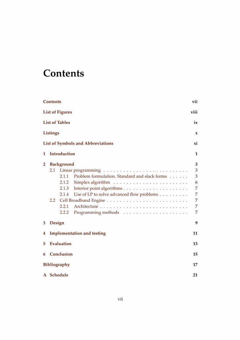
Contents

Contents vii

List of Figures viii

List of Tables ix

Listings x

List of Symbols and Abbreviations xi

1 Introduction 1

2 Background 32.1 Linear programming . . . . . . . . . . . . . . . . . . . . . . . . . . 3

2.1.1 Problem formulation. Standard and slack forms . . . . . . 32.1.2 Simplex algorithm . . . . . . . . . . . . . . . . . . . . . . . 62.1.3 Interior point algorithms . . . . . . . . . . . . . . . . . . . . 72.1.4 Use of LP to solve advanced flow problems . . . . . . . . . 7

2.2 Cell Broadband Engine . . . . . . . . . . . . . . . . . . . . . . . . . 72.2.1 Architecture . . . . . . . . . . . . . . . . . . . . . . . . . . . 72.2.2 Programming methods . . . . . . . . . . . . . . . . . . . . 7

3 Design 9

4 Implementation and testing 11

5 Evaluation 13

6 Conclusion 15

Bibliography 17

A Schedule 21

vii

List of Figures

viii

List of Tables

ix

Listings

x

List of Symbolsand Abbreviations

Abbreviation Description Definition

LP Linear programming page 3

xi

Chapter 1Introduction

(TODO)

1

Chapter 2Background

(TODO) Chapter introduc-tion

2.1 Linear programming

(Natvig) Do we need sectionintroductions too?This section is primarily based on [?] and [?].

2.1.1 Problem formulation. Standard and slack forms

The term linear programming (LP) refers to a type of optimisation problems inwhich one seeks to maximise or minimise the value of a linear function of aset of variables1. The values of the variables are constrained by a set of linearequations and/or inequalities. Linear programming is a fairly general problemtype, and many important problems (TODO) can be cast as LP problems — for (other than those

problems that areinitially formulatedas an LP problem)

instance, network flow problems and shortest path problems (see [?]).An example of a simple linear programming problem would be a factory that

makes two kinds of products based on two different raw materials. The profitthe company makes per unit of product A is $10.00, and the profit of productB is $12.50. Producing one unit of A requires 2 units of raw material R and 3units of raw material S; one unit of B requires 3 units of R and 1.5 units of S. Thecompany possesses 100 units of raw material R and 50 units of raw material S.We make the simplifying assumptions that all prices are constant and cannot beaffected by the company, and that the company is capable of selling everything itproduces. The company’s goal is to maximise the profit, which can be describedas 10.00x1 + 12.50x2 where x1 is the number of units of product A and x2 is thenumber of units of product B. The following constraints are in effect:

1Hence, LP is not (as the name would seem to suggest) a programming technique.

3

4 CHAPTER 2. BACKGROUND

• 2x1 + 3x2 ≤ 100 (the production of A and B cannot consume more units ofraw material R than the company possesses)

• 3x1 + 1.5x2 ≤ 50 (same for raw material S)

• x1, x2 ≥ 0 (the company cannot produce negative amounts of its products)

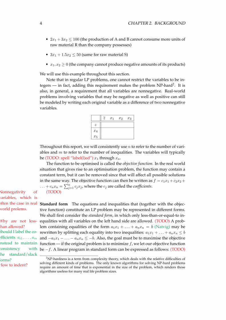
We will use this example throughout this section.Note that in regular LP problems, one cannot restrict the variables to be in-

tegers — in fact, adding this requirement makes the problem NP-hard2. It isalso, in general, a requirement that all variables are nonnegative. Real-worldproblems involving variables that may be negative as well as positive can stillbe modeled by writing each original variable as a difference of two nonnegativevariables.

z x1 x2 x3

z

x4

x5

Throughout this report, we will consistently use n to refer to the number of vari-ables and m to refer to the number of inequalities. The variables will typicallybe (TODO: spell “label(l)ed”) x1 through xn.

The function to be optimised is called the objective function. In the real worldsituation that gives rise to an optimisation problem, the function may contain aconstant term, but it can be removed since that will affect all possible solutionsin the same way. The objective function can then be written as f = c1x1 + c2x2 +. . . + cnxn =

∑nj=1 cjxj , where the cj are called the coefficients.

(TODO)Nonnegativity ofvariables, which isoften the case in realworld prolems.

Standard form The equations and inequalities that (together with the objec-tive function) constitute an LP problem may be represented in different forms.We shall first consider the standard form, in which only less-than-or-equal-to in-equalities with all variables on the left hand side are allowed. (TODO) A prob-Why are not less-

than allowed? lem containing equalities of the form a1x1 + . . . + anxn = b (Natvig) may beShould I label the co-efficients ai1, . . . , ain

instead to maintainconsistency withthe standard/slackforms?

rewritten by splitting each equality into two inequalities: a1x1 + . . . + anxn ≤ b

and −a1x1 − . . .− anxn ≤ −b. Also, the goal must be to maximise the objectivefunction — if the original problem is to minimize f , we let our objective functionbe −f . A linear program in standard form can be expressed as follows: (TODO)

How to indent?

2NP-hardness is a term from complexity theory, which deals with the relative difficulties ofsolving different kinds of problems. The only known algorithms for solving NP-hard problemsrequire an amount of time that is exponential in the size of the problem, which renders thosealgorithms useless for many real life problem sizes.

2.1. LINEAR PROGRAMMING 5

Maximise

f =n∑

j=1

cjxj

with respect to

n∑j=1

aijxj ≤ bi, for i = 1, . . . ,m.

x1, . . . , xn ≤ 0

Slack form The other common representation is slack form, which only allowsa set of equations (and a nonnegativity constraint for each variable). An in-equality of the form a1x1 + . . . + anxn ≤ b is converted to an equation byadding a slack variable w. Together with the condition that w ≥ 0, the equa-tion a1x1 + . . . + anxn + w = b is equivalent to the original inequality (whosedifference, or “slack”, between the left and right hand sides is represented byw). A linear program in slack form can be expressed as follows:

Maximise

f =n∑

j=1

cjxj

with respect to

wi = bi −n∑

j=1

aijxj , for i = 1, . . . ,m.

x1, . . . , xn ≤ 0

A proposed solution of a linear program (that is, a specification of a valuefor each variable) is called:

Feasible if it does not violate any of the constraints

Infeasible if it violates any constraint

Basic (TODO)

Optimal if it is feasible and no other feasible solutions yield a higher value forthe objective function

(TODO) The ??? theorem((TODO: citation))states that the op-timal solution of alinear program, if itexists, occurs whenm variables are setto zero and the n

others are nonzero.CHECK

6 CHAPTER 2. BACKGROUND

2.1.2 Simplex algorithm

The simplex algorithm, developed by (TODO)[?], was the (TODO) systematic al-

??? Dantzigfirst?

gorithm developed for solving linear programs. It requires the program to be inslack form. (TODO) The nonnegativity constraints are not represented explicitlyanywhere. (TODO)

Tableaux The variables in the leftmost column are referred to as the basic vari-ables, and the variables inside the tableau are called nonbasic variables. At anystage of the algorithm, the set of the indices of the basic variables is denotedB, and the set of nonbasic indices is denoted N . It should be noted that theslack form must have been created from a standard form, because this ensuresthat there are m slack variables, where each slack variable occurs in excactly oneequation. Initially, the set of basic variables is the set of slack variables, and thesizes of the basic and nonbasic sets are constant, with |B| = m and |N | = n.

For now, let us assume that the solution that is obtained by setting all non-basic variables to zero is feasible (which is the case only if none of the bi arenegative); we will remove this restriction later. This trivial solution will pro-vide a lower bound for the value of the objective function (namely, the constantterm). We will now select one nonbasic variable xj and consider what happensif we increase its value (since all nonbasic variables are currently zero, we can-not decrease any of them). Since our goal is to maximise the objective function,we should select a variable whose coefficient cj in the objective function is pos-itive. If no such variables exist, we cannot increase the objective function valuefurther, and the current solution (the one obtained by setting all nonbasic vari-ables to zero, so that f = c0) is optimal — we can be certain of this since linearfunctions do not have local maxima.

It seems reasonable to select the variable with the greatest coefficient, say,xl. How far can we increase this variable? Recall that each line in the tableauexpresses one basic variable as a function of all the nonbasic variables; hence wecan increase xl until one of the basic variables becomes zero. Let us look at rowi. If aij is negative, the value of wi will decrease as xl increases, so the largestallowable increase is limited by the current value of wi — which is bi, since allnonbasic variables were set to zero. Thus, by setting xl = − bi

aij, wi becomes

zero. However, other equations may impose stricter conditions. By looking atall rows where aij is negative, we can determine min

(− bi

ail

)and set xj equal

to it. If all ail are nonnegative, we can increase xl indefinitely without any wi

ever becoming negative, and in that case, we have determined the program tobe unbounded; the algorithm should report this to the user and terminate.

The next step, called pivoting, is an operation that exchanges a nonbasic vari-able and a basic variable. The purpose of pivoting is to produce a new situationin which no bi is negative, so that we can repeat the previous steps all over again.

2.2. CELL BROADBAND ENGINE 7

The nonbasic variable that was selected to be increased, xj , is called the enteringvariable, since it is about to enter the collection of basic variables. The leavingvariable to be removed from said collection. (TODO) We can eliminate the en- how to find it?tering variable from (and introduce the leaving variable into) the set of nonbasicvariables (the “main” part of the tableau) by rewriting the selected equation andadding appropriate multiples of it to each of the other equations:

Initialisation

The algorithm presented so far is capable of solving linear programs whose ini-tial basic solution (the one obtained by setting all nonbasic variables to 0) isfeasible. (TODO) This may not always be the case. We get around this by intro- Phase I and Phase IIducing an auxiliary problem which based on the initial problem that is guaranteed

Degeneracy

Example

We will now demonstrate one iteration of the simplex algorithm, on the follow-ing problem: (TODO)

2.1.3 Interior point algorithms

2.1.4 Use of LP to solve advanced flow problems

(TODO) Consult Miriam onthis

2.2 Cell Broadband Engine

2.2.1 Architecture

2.2.2 Programming methods

Chapter 3Design

(TODO)

9

Chapter 4Implementation and testing

(TODO)

11

Chapter 5Evaluation

(TODO)

13

Chapter 6Conclusion

(TODO)

Future work

15

Bibliography

17

Appendices

19

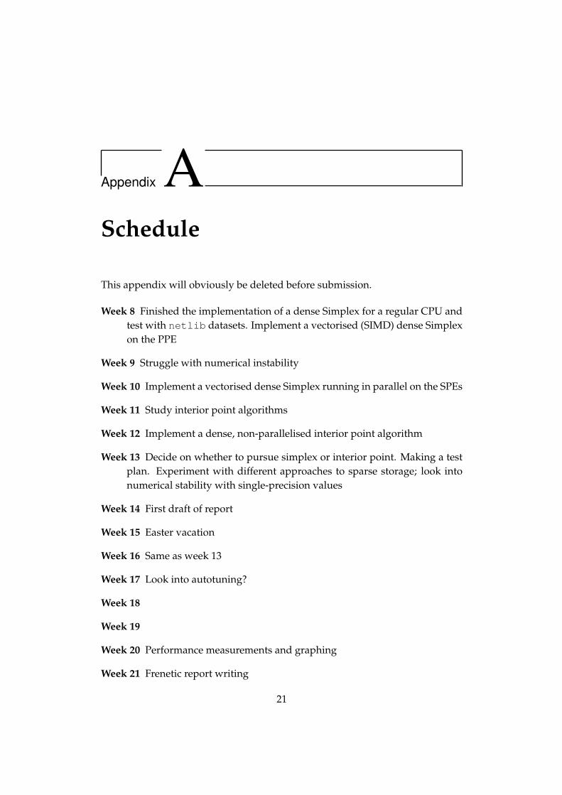
Appendix ASchedule

This appendix will obviously be deleted before submission.

Week 8 Finished the implementation of a dense Simplex for a regular CPU andtest with netlib datasets. Implement a vectorised (SIMD) dense Simplexon the PPE

Week 9 Struggle with numerical instability

Week 10 Implement a vectorised dense Simplex running in parallel on the SPEs

Week 11 Study interior point algorithms

Week 12 Implement a dense, non-parallelised interior point algorithm

Week 13 Decide on whether to pursue simplex or interior point. Making a testplan. Experiment with different approaches to sparse storage; look intonumerical stability with single-precision values

Week 14 First draft of report

Week 15 Easter vacation

Week 16 Same as week 13

Week 17 Look into autotuning?

Week 18

Week 19

Week 20 Performance measurements and graphing

Week 21 Frenetic report writing

21

22 APPENDIX A. SCHEDULE

Week 22 — “ —

Week 23 Ordinary submission deadline. Will try to submit as close to this dateas possible

Week 24

Week 25

Week 26

Week 27 Natvig goes on vacation

Week 28

Week 29 Final deadline: July 19