Linear Programming Fundamentals - Georgia State …dscthw/8140/LP1-2010.pdf · Linear Programming...

Linear Programming FundamentalsBy Thomas Whalen and Jeff Churchill

Spring 2010

A chicken farmer near Gainsville, Georgia would like to feed his flock properly, but as economically as possible. Ifhe had 50, or even 5,000 chickens, he would undoubtedly go down to the local feed and seed emporium. With500,000 chickens, a few cents per pound of feed adds up to serious money over a year's time. Nutritional require-ments are well known (and don't include marigold petals). A wide variety of types and grades of grains and mealsare capable of contributing important parts of these nutritional requirements. To complicate things further, most ofthese are commodity items whose market prices change daily and even hourly. What mix of various grades of corn,wheat, oat, millet, other grains, and supplements can he put through his feed mill to give him fat, healthy birds atleast cost?

A major distributor of consumer electronics has 8 warehouses serving 325 retail outlets scattered around thecontiguous United States. With the normal order/reorder cycle, supplies of the various products the company stocksin these warehouses can vary fairly dramatically. Similarly, the retail outlets experience their own fluctuations. Inthe fiercely competitive consumer electronics business, no stock equates to no sale. Any warehouse can ship to theBoise retail store to meet that store's need for six 19" SoSory modular color TV's if that warehouse has that many instock. Some can do it a lot more cheaply than others. Bozeman might need 4 sets too. Reno, the nearest warehouseto both stores, has 8. Repeat this scenario across 7 more warehouses and 323 more stores. Take into account (atleast), motor freight, UPS and its competitors, and air freight, all with differing rate structures among all pairs ofpoints. Is there a way to work out a least cost shipping schedule each week in time for it to matter?

MacroSoft Software is preparing to "roll out" its new killer application, a work processing package namedDRUDGE. It has identified the demographic characteristics of people who should be in the core market forDRUDGE, and has estimates of how many of these people live in each of the 17 major market areas they havetargeted. They have also identified a long list of print and broadcast media in which they might advertise DRUDGEduring the introduction. For each medium, they have information on the demographic "reach" in each of thesemarket areas, and a list of advertising rates. No matter how powerful any one medium may be, they have set somecriteria for maintaining a balance among them. With a $25,000,000 advertising budget for the rollout, how can theymaximize their total exposure to targeted potential customers?

All of these situations, and many many more, have some things in common. In each case, there is a well definedgoal; something that the decision maker wants to maximize (e.g., exposures to qualified buyers) or to minimize(e.g., the cost of shipping consumer electronics products). In each case, there are limitations that the decision makeris constrained to obey. The chicken farmer needs to meet nutritional requirements with an appropriate volume of amix that the chickens won't refuse to eat. The more #2 red winter wheat he includes in his mix, the less he can useof other potential ingredients. The distributor must meet its retailers' orders, and can't ship the same stereo system to2 different stores or leave a warehouse with a negative supply of Boogie Boxes. MacroSoft can't spend it all on TV(some "influentials" never watch), and a dollar they spend in InfoWorld isn't available to spend in PlayGirl. In allof these cases, there are tradeoffs. In all of these cases the relationships are really fairly simple, but there are somany to keep track of that it might seem mind boggling to the decision maker.

Linear Programming (LP) is a modeling approach for what is termed constrained optimization. As the term mightseem to imply, constrained optimization involves selecting a provably best solution in a situation where you areconstrained in some specific ways. There are a number of constrained optimization techniques, most of which fallunder the heading Mathematical Programming. Mathematical programming encompasses Linear Programming,Integer Programming, Quadratic Programming, and more. Of all of these, the least complex and most widelyapplied modeling approach is Linear Programming.

1

Programming in this context does not imply computer programming, despite the fact that the first digital computeractually put into use was constructed so that George Dantzig, the "father" of Linear Programming, could solve largelinear programming problems. The term "programming" is used here to imply developing a program of action in adecision situation.

The word linear is critical here. Linear programming solution methods depend on all relationships in the modelbeing linear. "Linear" means that all variables appear in every equation or inequality with a coefficient that is (orrepresents) a numeric constant and with an exponent of 1. The coefficient may be positive, negative, 0, or 1. If yougraph a linear equation or inequality, it is always a straight line (or, beyond 2 dimensions, a flat plane). Terms

involving the equivalent of X2, XY, , or are all examples of forms that you never see in a properlyXY

X12X25X3

4Yset up linear programming problem. If the real world problem requires non - linear relationships in order todescribe the situation correctly, it calls for a model other than linear programming to solve the problem.

The basic form of a linear programming problem involves maximizing or minimizing a linear objective functionsubject to a set of linear constraints. The classic mathematical form for such a problem is:

0 >all Xi

bm<amnXn . ..

am2X2+am1X1 +

. .

. ..

. . .. ..

. . . . . .

b2<a2nXn . ..

a22X2+a21X1 +

b1<a1nXn . ..

a12X2+a11X1 +

Subject to:

CnXn . ..

C2X2+C1 X1 +Maximize Z=

This is only symbolic of a linear programming problem so that we can identify its components. It is not literally anLP problem as we will deal with them. Normally, our problems will not appear so starkly mathematical. Youprobably find that to be a relief.

This format symbolizes a typical Maximization problem with n activity variables (the Xi values) and with mconstraints (the inequalities). The function Z is the objective function, and the Ci values are the objective functioncoefficients. When the problem has been solved, Z will be the total value of the objective function. We want Z tohave the largest value possible.

The Xi values represent the activity variables. Usually, these days, we use meaningful variable names like TV orWHEAT instead of Xi. when we set up the problem. An activity variable is a measure of the quantity of some activ-ity we will undertake as a result of our LP solution. Shipping a TV or buying a carload of wheat is an activity inthis sense. The other name we often use for these variables is decision variables. When we solve an LP problem,our principal result is values for all of the Xi's. That set of values is, if we formulated and solved our linearprogramming problem correctly, the optimal decision or optimal solution. All variables (we will later see otherkinds) are restricted to being zero or positive. This is very helpful in creating a way to solve these problems. It alsousually makes good physical sense. You can't make, e.g., negative stereos. You might think of disassembling oneto make its parts available for another product as making a "negative" stereo, but I challenge you to find a way toget the assembly labor back out of the stereo and use it in another product!

2

Assumptions behind linear programmingThere are some very important assumptions underlying our use of linear programming. As with all models, weassume that our model is a close enough analogy to the real situation that we can let it help guide our decisionmaking. We also have some assumptions that are specific to LP.

Linearity We assume that the underlying relationships we describe are linear. This means for examplethat there are no increasing or decreasing returns to scale. If we purchase parts or materials, we are not ignor-ing discounts that change with volume. This is simply the assumption that the relationships we describe aslinear are in fact linear.

Additivity This assumption requires internal consistency in our units of measure. Translated intoEnglish, if we add apples to walnuts to marshmallows we may have Waldorf Salad but we do not have aviable LP objective function or constraint. For example, if one objective function coefficient is in $, anotherin Y--, another in F, another in £, and yet another in DM, well, it's all money isn't it? But how much is $100 +Y--1500 + 850F + £144 + 1900DM??? Or on the left hand side of a constraint if we have 2 hours/Widget 4hours + 3 Fidgets/hour 6 Fidgets, just what does the resulting 26 mean?

Non Negativity We saw an implication of this assumption when we looked at the basic format for an LPproblem. All variables are restricted to values greater than or equal to zero. This seldom poses a problem. Inthe rare case where we might have a legitimate need for a variable to take on a negative value, there is a trickfor evading this requirement. You might see it if you take a more advanced course, but we won't consider ithere.

Certainty Our solution methods become meaningless if we are uncertain of the values of the coeffi-cients. The certainty assumption simply assumes that they aren't random variables. As we get deeper into LP,we will learn how we can avoid being overly restricted by this requirement.

Divisibility We must be willing to accept and implement solutions that are not whole numbers. 142.25tons of wheat seldom bothers anybody, but 76.180375 trombones don't seem to lead very many students'parades, 12345.6789 table lamps seems a real curiosity, and of a nuclear submarine seems a chilling way to

34

spend one's hard earned tax dollars. For wheat, we have no problem. The trombones are easier to cope withif we see this number as a rate, not a quantity. Another way of really saying about the same thing is to saythat the .180375 trombone isn't scrap brass, but work in process that will be completed in the next operatingperiod. If LP tells us to make 12345.6789 table lamps next year, there is no point in worrying. By the end ofthe year, many things will have happened to revise that, so it is really only a fairly approximate target to worktoward. .6789 of a table lamp represents a very small amount of the total value involved anyway. In the caseof the fractional submarine, we probably need to drop LP and try Integer Programming. It's hard to justifyrounding to the nearest $10,000,000,000.

3

A Very Simple Linear Maximization Problem

Case 1: Widgets and Gadgets (Unpainted)A widget takes 4 hours to assembleA gadget takes 8 hours to assemble

If W is the number of widgets produced and G is the number of gadgets produced, the number of hours of assemblytime required is 4W + 8G

A maximum of 720 assembly hours are available per eight hour day since your factory can only accommodate 90workers in the assembly area.

4W + 8G < 720

Each widget earns $50 contribution to profit and overhead. The contribution of gadgets varies from month tomonth; some months it is as low as $20 per gadget while other months it is as high as $110.

All widgets and gadgets are sold immediately at the going rate; none are kept in inventory.

In the following graph, the horizontal axis represents the number of widgets produced, and the vertical line repre-sents the number of gadgets produced. Every point in the graph represents a "production schedule" calling forproducing a number of widgets equal to the horizontal coordinate of the point, and a number of gadgets equal to thevertical coordinate of the same point. Points outside the shaded triangular area are "infeasable" in the sense thatthere are not enough assembly hours available to produce that many widgets and gadgets. The shaded area is calledthe "feasible region" because every point in its interior or its boundary represents a sensible production schedule inthe sense that there are enough assembly hours available to actually produce that many widgets and gadgets.

0 50 100 150 2000

50

100

150

200

Widgets

Gad

gets

QUESTION:how many widgets and gadgets should you produce per day?

ANSWER: if the contribution per gadget is more than $100, produce 90 gadgets and no widgets. If the contributionper gadget is less than $100, produce 180 widgets and no gadgets.

(This problem is so simple that there's really no need for anything a powerful as linear programming, but it illus-trates the barest essentials of an LP problem.)

4

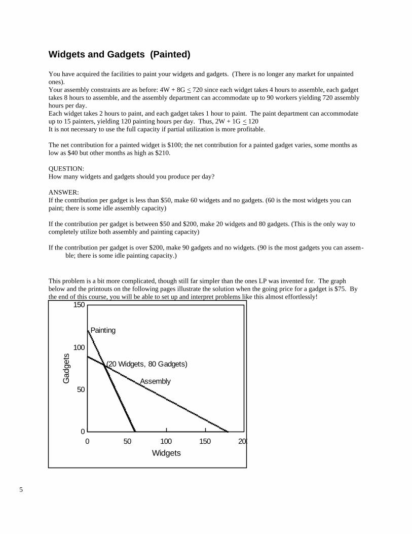
Widgets and Gadgets (Painted)

You have acquired the facilities to paint your widgets and gadgets. (There is no longer any market for unpaintedones).Your assembly constraints are as before: 4W + 8G < 720 since each widget takes 4 hours to assemble, each gadgettakes 8 hours to assemble, and the assembly department can accommodate up to 90 workers yielding 720 assemblyhours per day.Each widget takes 2 hours to paint, and each gadget takes 1 hour to paint. The paint department can accommodateup to 15 painters, yielding 120 painting hours per day. Thus, 2W + 1G < 120It is not necessary to use the full capacity if partial utilization is more profitable.

The net contribution for a painted widget is $100; the net contribution for a painted gadget varies, some months aslow as $40 but other months as high as $210.

QUESTION:How many widgets and gadgets should you produce per day?

ANSWER:If the contribution per gadget is less than $50, make 60 widgets and no gadgets. (60 is the most widgets you canpaint; there is some idle assembly capacity)

If the contribution per gadget is between $50 and $200, make 20 widgets and 80 gadgets. (This is the only way tocompletely utilize both assembly and painting capacity)

If the contribution per gadget is over $200, make 90 gadgets and no widgets. (90 is the most gadgets you can assem-ble; there is some idle painting capacity.)

This problem is a bit more complicated, though still far simpler than the ones LP was invented for. The graphbelow and the printouts on the following pages illustrate the solution when the going price for a gadget is $75. Bythe end of this course, you will be able to set up and interpret problems like this almost effortlessly!

0 50 100 150 2000

50

100

150

Painting

Assembly

(20 Widgets, 80 Gadgets)

Widgets

Gad

gets

5

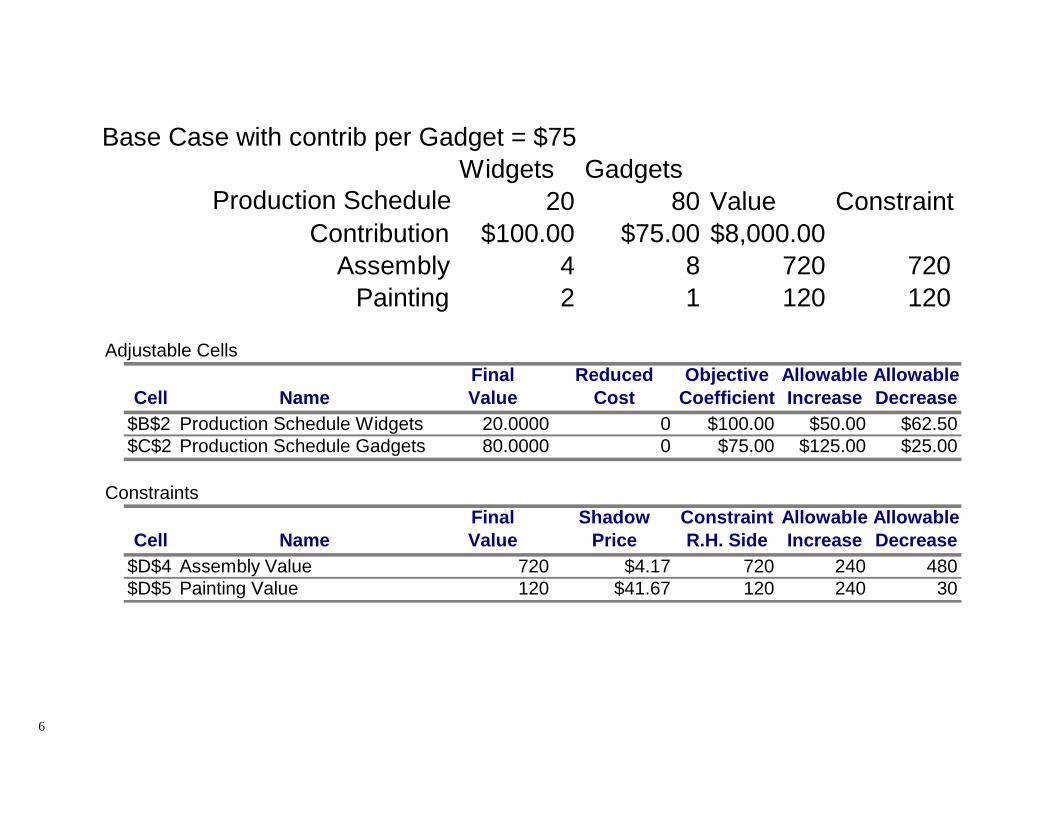
Base Case with contrib per Gadget = $75Widgets Gadgets

Production Schedule 20 80 Value ConstraintContribution $100.00 $75.00 $8,000.00

Assembly 4 8 720 720Painting 2 1 120 120

6

Adjustable CellsFinal Reduced Objective Allowable Allowable

Cell Name Value Cost Coefficient Increase Decrease

$B$2 Production Schedule Widgets 20.0000 0 $100.00 $50.00 $62.50$C$2 Production Schedule Gadgets 80.0000 0 $75.00 $125.00 $25.00

ConstraintsFinal Shadow Constraint Allowable Allowable

Cell Name Value Price R.H. Side Increase Decrease

$D$4 Assembly Value 720 $4.17 720 240 480$D$5 Painting Value 120 $41.67 120 240 30

Effect of One Additional Assembly HourWidgets Gadgets

Production Schedule 19.91667 80.16667 Value ConstraintContribution $100.00 $75.00 $8,004.17


7

Effect of One Additional Assembly WorkstationWidgets Gadgets





$D$3 Production Schedule Widgets 19.3333 0 $100.00 $50.00 $62.50$E$3 Production Schedule Gadgets 81.3333 0 $75.00 $125.00 $25.00



$F$5 Assembly Value 728 $4.17 728 232 488$F$6 Painting Value 120 $41.67 120 244 29

8

Effect of One Additional Painting WorkstationWidgets Gadgets





$D$3 Production Schedule Widgets 25.3333 0 $100.00 $50.00 $62.50$E$3 Production Schedule Gadgets 77.3333 0 $75.00 $125.00 $25.00



$F$5 Assembly Value 720 $4.17 720 304 464$F$6 Painting Value 128 $41.67 128 232 38

9

Effect of a Redundant Constraint

MAX 100 WIDGETS + 75 GADGETS SUBJECT TO 2) 4 WIDGETS + 8 GADGETS <= 720 3) 2 WIDGETS + GADGETS <= 120 4) WIDGETS + GADGETS <= 101

OBJECTIVE FUNCTION VALUE 1) 8000.00000

$25.00$125.00$75.00$0.0080Gadgets$62.50$50.00$100.00$0.0020WidgetsDereaseIncrease

AllowableCurrentCoeff

ReducedCost

ValueVari-able

1Infinity101$0.0014303120$41.670348012720$4.1702

DereaseIncreaseAllowableCurrent

RHSDualPrice

Slack orSurplus

Row

Effect of a "Small" Increase in Gadget Contribution MAX 100 WIDGETS + 195 GADGETSSUBJECT TO 2) 4 WIDGETS + 8 GADGETS <= 720 3) 2 WIDGETS + GADGETS <= 120

OBJECTIVE FUNCTION VALUE 1) $17,600.00



ReducedCost

ValueVari-able

30240120$1.6703480240720$24.1702


RHSDualPrice

Slack orSurplus

Row

Effect of a Degenerate Constraint

MAX 100 WIDGETS + 75 GADGETS SUBJECT TO 2) 4 WIDGETS + 8 GADGETS <= 720 3) 2 WIDGETS + GADGETS <= 120 4) WIDGETS + GADGETS <= 100

OBJECTIVE FUNCTION VALUE 1) 8000.00000



ReducedCost

ValueVari-able

400100$50.0004080120$25.00030Infinity720$0.0002


RHSDualPrice

Slack orSurplus

Row

Effect of a "Large" Increase in Gadget Contribution MAX 100 WIDGETS + 205 GADGETSSUBJECT TO 2) 4 WIDGETS + 8 GADGETS <= 720 3) 2 WIDGETS + GADGETS <= 120

OBJECTIVE FUNCTION VALUE 1) $18,450

$5.00Infinity$205.00$0.0090GadgetsInfinity$2.50$100.00($2.50)0WidgetsDereaseIncrease


ReducedCost

ValueVari-able

30Infinity120$0.00303720240720$25.62502


RHSDualPrice

Slack orSurplus

Row

10

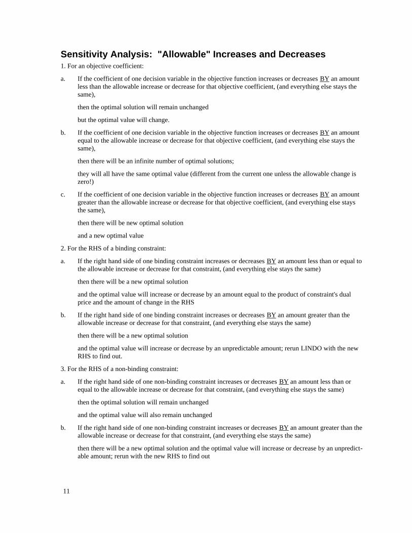
Sensitivity Analysis: "Allowable" Increases and Decreases1. For an objective coefficient:

a. If the coefficient of one decision variable in the objective function increases or decreases BY an amountless than the allowable increase or decrease for that objective coefficient, (and everything else stays thesame),

then the optimal solution will remain unchanged

but the optimal value will change.

b. If the coefficient of one decision variable in the objective function increases or decreases BY an amountequal to the allowable increase or decrease for that objective coefficient, (and everything else stays thesame),

then there will be an infinite number of optimal solutions;

they will all have the same optimal value (different from the current one unless the allowable change iszero!)

c. If the coefficient of one decision variable in the objective function increases or decreases BY an amountgreater than the allowable increase or decrease for that objective coefficient, (and everything else staysthe same),

then there will be new optimal solution

and a new optimal value

2. For the RHS of a binding constraint:

a. If the right hand side of one binding constraint increases or decreases BY an amount less than or equal tothe allowable increase or decrease for that constraint, (and everything else stays the same)

then there will be a new optimal solution

and the optimal value will increase or decrease by an amount equal to the product of constraint's dualprice and the amount of change in the RHS

b. If the right hand side of one binding constraint increases or decreases BY an amount greater than theallowable increase or decrease for that constraint, (and everything else stays the same)

then there will be a new optimal solution

and the optimal value will increase or decrease by an unpredictable amount; rerun LINDO with the newRHS to find out.

3. For the RHS of a non-binding constraint:

a. If the right hand side of one non-binding constraint increases or decreases BY an amount less than orequal to the allowable increase or decrease for that constraint, (and everything else stays the same)

then the optimal solution will remain unchanged

and the optimal value will also remain unchanged

b. If the right hand side of one non-binding constraint increases or decreases BY an amount greater than theallowable increase or decrease for that constraint, (and everything else stays the same)

then there will be a new optimal solution and the optimal value will increase or decrease by an unpredict-able amount; rerun with the new RHS to find out

11

"Allowable" Increases and Decreases

Changed (Rerun to find thenew )Optimal Payoff)

ChangedMore than“Allowable”

UnchangedUnchangedEqual to“Allowable”

UnchangedUnchangedLess then“Allowable”Right-Hand-Side

of Non-BindingConstraint(Shadow Price =0)

Changed (Rerun to find thenew Optimal Payoff)


Shadow Price of theconstraint times thechange in its RHS

ChangedEqual to“Allowable”

Sadow Price of theconstraint times thechange in its RHS

ChangedLess then“Allowable”

Right-Hand-Sideof BindingConstraint(Shadow PriceNot = 0)

Changed (Rerun to find thenew Optimal Payoff)


Quantity of X times the changein its objective coefficient

An infinite number of solutions(including the old one)

Equal to“Allowable”

Quantity of X times the changein its objective coefficient

UnchangedLess then“Allowable”Objective Coeffi-

cient of DecisionVariable “X”

Change in Optimal PayoffOptimal DecisionAmount itIncreases orDecreases BY

Quantity

12

Case 2: Beau Jarble's Maximization ProblemBeau Jarble has a small plant in which he makes a very limited line of inexpensive "mag" wheels for cars in theSecret Car Club of America (SCCA) Impound Touring category. All his wheels are 7" wide, and are drilledfor either 4 or 5 wheel studs (for attaching the wheels). He purchases "blank" wheels cast to his design by alocal foundry and finishes them in his little plant on weekends off from his regular job, using part time workersfor labor. His part timers are all first rate machinists who earn $30 an hour.

The ITA model is made from a 13" diameter by 7" wide "A" casting and sells for $125. The ITS model, forheavier and more powerful cars, is made from the 14" by 7" "S" casting and sells for $145. His present stock ofcastings cost him $50 each for the A units and $57.50 each for the S units, but due to a drop in the price ofaluminum he can get his next batch at $45 and $50. He has a good stock of castings on hand and considers thefoundry to be utterly reliable. He does not anticipate being limited by the casting supply.

His wheels are highly regarded by both real racers and "cafe racers". While demand is certainly not unlimited,he figures he could sell all the ITA wheels he could possibly make. He does not think that he could sell morethan 25 sets of ITS wheels per week. On the other hand, to maintain the prestige of his product, he never wantsto sell more ITA than ITS.

The first operation in making a casting into a wheel is to use a milling machine to put a properly aligned flatsurface on the back of the wheel where it mounts to the car. He has 3 milling machines and 3 operators whoeach work up to 10 hours per weekend. They are each able to "backface" 5 wheels per hour.

The next step is to drill the wheel mounting holes on a special drill press. An ITA wheel requires 4 holes, andan ITS wheel needs 5. His drill press operator can drill 60 holes/hour and is willing to work as many as 10hours in a weekend. Once the wheels have their mounting holes drilled, they can go on a lathe to be trued andsurface finished. Beau has 3 lathes and operators who each can work 10 hours on a weekend. It takes 18minutes to perform all needed operations on an ITA, and 12 minutes on an ITS.

The last major operation is drilling the valve stem hole in each wheel. Beau does this himself on another drillpress. It takes very little time, but requires a special stepped bit that costs $125 and is worn out after drilling120 to 130 wheels. This weekend he has one new bit on hand, his old one is worn out, and he's ordered anotherthat won't arrive before next Wednesday.

Beau does some final finishing and packaging himself. The materials for this work cost $12 for an ITA wheeland $ 19.50 for an ITS. His accountant takes $1/wheel depreciation on each of his machines, and figures otheroverhead at $10/wheel.

Beau would like to put together a practical production schedule for this weekend that would maximize profit forhim. His friend Willy Wonky claims to know all about LP, and has offered to find Beau's best mix of wheelsthat way. Before you turn the page, why not get out a piece of paper and see if you can formulate this problem.I bet you can do better than Willy!

13

Willy went to work, and came back to see Beau after a couple of hours. First he showed Beau how he figuredwhat to minimize:

$103.50$91.00AccountingCost

$10.00$10.00Overhead$1.00$1.00Depreciation$19.50$12.00Final$1.00$1.00Stem$6.00$9.00Lathe$2.50$2.00Drilling$6.00$6.00Backfacing$57.50$50.00CastingITSITA

This, he said, set him up for this formulation of the problem:

Stem100<25 ITS ITA -

Lathe30< 12 ITS18 ITA +

Holes60< 5 ITS 4 ITA +

Backface30< 5 ITS 5 ITA + Prestige0= ITS - ITA +

Demand25< ITSSubject to:

103.5 ITS91 ITA +Minimize Z=

Beau knows better than this! Willy's formulation is wonky 9 ways from Sunday. There are a few mistakes thatWilly didn't make, but most of the ones he missed, he only missed because Beau's problem didn't provide himthe opportunity to commit the particular error.

We don't want to be as wonky as Willie, so let's interrupt this problem to look at a few basic principles forformulating LP problems. We won't hit everything, but what we will look at will be important.

14

Objective function In linear programming problems, our activity variables must always be things on which the decision maker canact directly and which affect achievement of his or her goal. Willie at least got this right. It appears that hisvariable ITA was intended to represent the number of ITA wheels to make this weekend, and ITS representedthe number of ITS wheels to make this weekend.

Correspondingly, the objective function should represent the effect on the variable that he or she wants tooptimize from acting on those things. Willie apparently thought that variable was cost. That is seldom, if everthe case when we can directly identify a revenue with the activity variable. If Beau wants to minimize cost, it iseasy. He can just go out of business. Voila! No cost! But, of course, also no revenue.

Generally, we minimize when there is a set of performance limitations we must stay within and wish to do so ascheaply or easily as possible. If Beau had a contract requiring him to deliver at least 100 wheels consisting ofany mix of ITA and/or ITS models for $13,000, then it would be in his interest to find the least costly mix thatwas feasible for him to make this weekend. His decision would not affect revenue as long as he met therequirements of the contract. But here, every wheel is going to bring in either $125 or $145. It is not in Beau'sbest interests to ignore those revenues.

Beau wants to maximize his profit. More specifically, he wants to maximize the total positive increment to hiseconomic well-being. He can seriously mislead himself if he takes into account in his objective functionanything that his decision cannot actually change. There is a rule we always try to apply when we attempt tomeasure the impact of a potential decision. We do not apply it only in linear programming, but we certainly dotry always to use the rule in formulating LP problems. It defines Decision Costs and Decision Revenues.

{ Include a cost or revenue if it represents a future cash flow that arises as a directconsequence of the decision being made.

The selling price of a wheel is a future cash flow that Beau will collect only if he makes and sells that wheel. Itqualifies.

Willie included some things that do not qualify. Accountants have some convenient fictions that may be usefulfor financial accounting purposes, but that have a strong barnyard odor when used for decision makingpurposes. These fictions are not wrong, but they are highly inappropriate (and therefore wrong) in mostdecision models. The fictions are:

1. The correct cost to use is some form of historical cost. For financial accounting this providesauditability and keeps the accountants from needing additional variance accounts. That is fine if itis your intent to measure past cash flow. From a decision making viewpoint, the value of an itemis what it will cost to replace it so as to remain a going concern. If you do not intend to remain agoing concern, estimated liquidation value, if any, is best.

2. Buildings and equipment must be depreciated. For financial accounting purposes, this allocatesthe cost of major items to the operating periods that they benefit. From a decision makingviewpoint, if we use it this period and it will still be there to use next period, it costs us nothing.What we paid for the item in the past is a sunk cost, even if the accountant chooses to allocate iton a per item manufactured basis. Beau's accountant allocated $1.00 per wheel. He or she couldhave just as logically allocated 25¢ per hole!

3. Overhead costs of manufacturing must be assigned to products. Some consider this rule to be alittle weird even for financial accounting purposes. These are period costs that will be incurred ifthe business is operating. Some are cash expenditures (the water bill, for example). Others areallocations like building depreciation. Even financial accountants know that, if a cost is directlytraceable to increments of product, it should be a line item charge against that product. Overheadcosts, by definition, do not arise from product mix decisions.

15

Good 'ol Willie managed to fall into all three of these traps. Let's get him out.

1. The wheel castings now on hand are a sunk cost. The only reason we want to treat them ascosting something is that when Beau has used them up, he will need to buy more in order to stayin business. When he buys more, he'll pay the new price. So that's what they're worth.

2. Willie charged the accountant's equipment depreciation figure to the wheels. To whom shouldBeau write the depreciation check? This is not a decision cost. We exclude it.

3. What are we going to do with Willie? He even charged overhead. WE know better. Out it goes.We're making decisions, not keeping books.

When we're done, here's what we've got:

$80$50ContributionMrgin

$85$75Marginal Cost$1$1Depreciation$20$12Final$1$1Stem$6$9Lathe$3$2Drilling$6$6Backfacing$58$50Casting

$145$125PriceITSITA

You should trace this through - each item we included is a direct future cash consequence of making and sellinga wheel.

16

ConstraintsLet's take another look at the constraints for Beau's problem as Willie formulated them:

Stem100< ITA -25 ITS6

Lathe30<+18 ITA 12 ITS5

Holes60<+ 4 ITA 5 ITS4

Backface30< + 5 ITA 5 ITS3 Prestige0= - ITA ITS2

Demand25< ITS1

I'm going to try to translate this into its units of measure; in other words, attempt a dimensional analysis. It mayreveal some problems.

100 Stem Holes< ITA+25 Sets ofITS ITS6

30 hours Lathe time<18( munitesPer ITA ) ITA+12( munites

Per ITS ) ITS5

60 holes on drill press<4( holesPer ITA ) ITA+5( holes

Per ITS ) ITS4

30 hours Backface on Mill<5( ITAPer Hour ) ITA+5( ITS

ITSPer Hour ) ITS3

0 Prestige=1prestigePer ITA ITA+1

prestigePer ITS ITS2

25 Sets of ITS<ITAITS1

I've numbered the constraints to make them easier to refer to. The problems are now much easier to see andthen to deal with. Taking each constraint in turn,

1. Incongruity arises here from comparing wheels and sets. Converting the RHS (Right Hand Side)to wheels will cure the problem.

2. Willie got this one correct dimensionally, but he fell into the common trap of over-constrainingthe solution. Beau didn't want to sell more ITA than ITS. Selling more ITS than ITA is just asgood as selling the same number.

3. The left hand side evaluates to , a nonsense quantity. It's pretty obvious that theITA2

hour ITS2

hourcoefficients should have been inverted.

4. The left hand side should be fine; it evaluates to holes drilled. The problem is in the RHS, whereWillie forgot to multiply by the available number of hours of drill press time.

5. The left hand side evaluates to minutes, while the RHS is in hours. Either will work, but mixingthem won't work worth a hoot.

6. Willie suffered from a couple of confusions here. He's back to mixing wheels and sets. Worse,for some reason he tried to combine 2 constraints into 1, causing both the ITS term and the RHSto be nonsense. He took one of Beau's simplest constraints and made it complicated.

Now that we know what the problems are, we can fix it pretty easily. Let's write the constraints the way wethink they should be, then test them with dimensional analysis. If you got them right to start with, congratula-tions! If you are unsure, use dimensional analysis to test them before you continue reading. Write theconstraints now, do the dimensional analysis check, then look at the rest of the page.

17

Stem125<+ ITA ITS

Lathe30<+ .3 ITA .2 ITS

Holes600<+ 4 ITA 5 ITS

Backface30<+ .2 ITA .2 ITS

Prestige0> - ITA ITS

Demand100< ITS

(I've written ITS before ITA here because I'm planning to graph ITS as the horizontal ("x") coordinate.)Before we examine this version of the constraints dimensionally, let's note a few things. If a decision variabledoes not affect a constraint, as in the first one, we may either omit it as you see here, or we may include it witha coefficient of 0. In both the first and the last constraint, no coefficients are visible. That does not mean thatthey aren't there. When we don't write a coefficient, a coefficient of 1 is implied. Some students whose mathbackground is not as strong as it should be seem to think that a coefficient of 0 is implied. Not so. Finally, thesecond and fourth constraints are in hours. If you (correctly) formulated them in minutes, you aren't wrong butjust made a different choice. You could, with difficulty, use seconds, fortnights, or decades.

Dimensionally, this is:

Stemholes<holes

Per ITA ITA+holes

Per ITS ITS

Lathehours<hours

per ITA ITA+hours

per ITS ITS

Holesholes<holes

Per ITA ITA+holes

Per ITS ITS

Backfacehours<hours

per ITA ITA+hours

per ITS ITS

PrestigePoints>points

per ITA ITA-pointsper ITS ITS

DemandITS< ITS

which resolves to

Stemholes<holes

Lathehours<hours

Holesholes<holes

Backfacehours<hours

Prestigepoints>points

DemandITS<ITS

which isn't all that exciting, but it is at least clear that we don't have constraints that are obvious nonsense.

18

The corrected maximization problemWhen we put together the corrections we have made, Beau's product mix problem is:

Stemstemholes125<+ ITA ITS

Lathehours30<+ .3 ITA .2 ITS

Holesholes600<+ 4 ITA 5 ITS

Backfacehours30<+ .2 ITA .2 ITS

Prestige"points"0> - ITA ITS

DemandITS100< ITSsubject to:

+50 ITA 60 ITSMaximize Z =

Willie didn't mention the non-negativity restriction that we saw when we looked at the mathematical form foran LP problem, and it isn't included here. Some people think that you should always write it. Maybe. On theother hand, it is inherent in the very fact that this is an LP problem, so we'll assume that while it is necessary toobey it, it is unnecessary to write it.To find Beau a usable solution, our first responsibility is to see to it that any proposed solution is feasible.

{ A feasible solution is one that does not violate any constraints, including non negativity.

In this case, a feasible solution is a number of ITA and ITS wheels that

ˆ includes either some or none of each product (Beau won't make wheels of antimatter!)

ˆ includes no more than 100 ITS

ˆ has at least as many ITS as ITA

ˆ requires no more than 30 hours of milling machine time to backface the wheels

ˆ requires the drill press operator to drill no more than 600 mounting holes in wheels

ˆ needs no more than 30 lathe hours for truing and surface finishing wheels

ˆ has Beau drilling valve stem holes in no more than a total of 125 wheels.

If you're sharp, you have already noticed that we are violating one of the assumptions of LP. Since the specialstepped drill bit can drill 120 to 130 holes, but we split the middle and said 125, we are violating the certaintyassumption. The possible risk here is that either at the end of the weekend he finds he could have made morewheels (with a different mix), or that he is stuck with up to 5 wheels that still need valve stem holes drilled. Amore conservative approach would have used 120 on the RHS, but given up some profit potential. Later, wewill see how to evaluate this. For now, let's just note that we sometimes knowingly violate this assumption, butshould always examine the possible consequences.

19

FEASIBLE SOLUTIONSIn effect, our inequalities (including the implied ITA > 0 and ITS > 0 ) define a "space", which we call thefeasible solution space. We must select a point in that space for Beau, and to do that we'll have to know whatpoints are members of that space. We're going to do that graphically. The graphical representation will help usto understand what LP does and how it works.

0 50 100 1500

50

100

150

Y N Demand

N YPresteige

Y N Backface

Y NHoles

Y NLathe

Y NStems

Feasible Region

itS Wheels

itA W

heel

s

Beau Jarble's Constraints

I used Y(es) and N(o) to show which side of each constraint line was infeasable. The open space at the bottom(labeled Feasible Region) contains all combinations of ITA and ITS wheels Beau can make this weekend. Anypoint inside this space, or on a boundary, represents a combination that will not violate any constraint. Anypoint that is not in this region violates at least one constraint.

Beau's problem presents us with some offbeat situations that we sometimes see. First, we have a redundantconstraint. Looking at the graph, we can see that the valve stem drilling constraint dominates the backfaceconstraint. The backface constraint lies entirely outside the feasible region that we would have if the special

20

valve stem drill were the only other constraint. In the olden days, when college students walked barefoot toclass through raging blizzards, we suggested that people try to spot and eliminate such constraints beforesolving LP problems. Now that we have high speed electronic confusers to do the drudge work, we leave themin. If Beau's valve stem drill turned out to be the special titanium version that can drill 1000 holes, we canconceive of the possibility that backfacing might become a binding constraint.

The other offbeat situation that we have is that this turns out to be a degenerate problem. This says nothingabout Beau's morals; that's a separate issue. Degeneracy can become a more complex issue when you havemore than 2 activity variables, but it is a simple one here. In a 2 dimensional space, the intersection of 2 linesdefines a point. But here, we have 3 constraint lines intersecting at ITA = 25, ITS = 100. This is one more linethan is needed to define a point in 2 dimensions.

No big deal, you say. We really have that point nailed. Yes, but . . . At one time, the mathematicians couldnot prove that the Simplex Method (we'll see it later) would always find a solution to a degenerate problem.Even today, when someone designs a computer program to solve LP problems with the Simplex Method, he orshe must take special precautions to deal with degeneracy.

Perhaps worse, we will see that an intersection on the boundary of the feasible region is a candidate to becomethe optimal solution. If this turns out to be the optimal solution (it will, though you have no way to know thatyet without peeking), then that complicates something we do after the problem is solved. After we solve an LPproblem, we usually have some interest in what is often called post-optimality analysis or sensitivity analysis.Sensitivity analysis is just a formalized way of playing "what if?". It is often the most important reason forsolving an LP problem, and sometimes is even the whole reason.

The most important (usually) kind of sensitivity analysis one might do on an LP solution is to ask "what wouldhappen if I could change the RHS of this constraint?". Degeneracy greatly complicates answering thisquestion. We must return to this issue after we have completed our solution.

Optimal solutionSomewhere in or on the edge of the feasible region is the very best combination of ITA and ITS wheels forBeau to make. Let's consider the point ITA = 40 and ITS = 60 (look for a little + near the top of the feasibleregion). Beau could make that combination, no sweat. He did just last weekend. Could it possibly be a candi-date for best combination?

He could make 10 more ITA wheels, gaining $50 for each, without giving up a single ITS wheel. He couldmake 10 more ITS wheels, gaining $60 for each, without giving up a single ITA wheel. In fact, he could moveto the point ITA = 50, ITS = 70 (10 more of each) and earn $1,100 more. If Beau were trying to minimize thecost of making wheels, he could make fewer of both kinds, thus reducing his total cost. This should lead us tothe realization that whether you want to maximize or minimize,

{ at an interior point in the feasible space, you can always find another point thatis better.

For this reason, we can eliminate the entire inside of the feasible space and restrict our search to its boundaries.That means that somewhere along some constraint line (remembering that non-negativity constrains us) theremust be the optimal point for which we are looking. That eliminates a whole lot of fruitless possibilities thatwe need not examine!

One way we might search is to set a target value for total contribution to overhead and profit and see whatcombinations of ITA and ITS might yield that contribution. That will generate a line that looks just like aconstraint line, except that we'll make it a dashed line so we can tell it from a constraint line. If it is so far fromthe origin that it doesn't touch the feasible space, then we'll try a smaller number. If it is so close to the originthat it runs right through the middle of the feasible solution space, we'll try a larger number.

21

We call these lines isoprofit lines. If we were minimizing cost, they would be isocost lines. The generic termfor isoprofit and isocost is isoquant. (The prefix iso comes from a Greek word meaning equal or same.) If weare maximizing, as we are now, we want the highest total contribution isoprofit line that has at least one feasi-ble point somewhere along it. If we are minimizing, then we would want the lowest total cost isocost line thathas at least one feasible point. As we try different levels of profit or cost, we will see that the lines are allparallel to each other. That makes things easier for us.

We draw an isoprofit line very much like we do a constraint, except that we must invent the number on theright side of the equation. We find 2 intercepts, and join them with a straight line. For a first try, I usually startwith the product of the objective function coefficients, because I know that will give me easy arithmetic infinding the intercepts. This time, I will start with a $50×$60 = $3000 isoprofit line.

50 ITA + 60 ITS = 3000ITA = 0, ITS = 50ITS = 0, ITA =60

If you look at the graph (next page), this is obviously too low. Let's triple it and see what we get.The process is the same; only the numbers change.

50 ITA + 60 ITS = 9000ITA = 0, ITS = 150ITS = 0, ITA = 180

This time I overshot and got no feasible points. Let's split the difference.

50 ITA + 60 ITS = 6000ITA = 0, ITS = 100ITS = 0, ITA = 120

That was a little too low, but it got me close enough that I could see that the highest isoprofit line had to passright through the intersection at ITS=100, ITA = 25. I just moved my straightedge parallel to the $6000isoprofit line and drew a partial final isoprofit line through that point. The total profit contribution at that pointis

50 ITA + 60 ITS = profit50 × 25 + 60 × 100 = 7250

We have found Beau's optimal solution. He should make 25 ITA wheels and 100 ITS wheels, for a total contri-bution of $7,250. Not bad for a weekend's work, but let's don't forget he has both overhead and a substantialinvestment. It is very rare that we can legitimately call the final objective function value "profit". Profit is anaccounting term, and we disdain financial accounting principles for decision purposes.

You will note that we found Beau's best product mix at an intersection of constraints. We call this a cornerpoint solution. The great breakthrough that made LP a practical problem solving tool instead of just an interest-ing mathematical structure was the proof of a theorem that permits us to focus on just the corner points. Whenyou demystify the theorem, the essence of what it says is that

{ In a feasible linear programming problem, there is no solution superior to thebest corner point solution.

In Beau's feasible region, there are only 5 corner points. What this theorem says is that one of them must be theoptimal solution. This is the cornerstone on which the Simplex method, which permits us to solve problemswith many variables, is built.

22

0 50 100 1500

50

100

150

Y N Demand

N Y

Presteige

Y N Backface

Y N

Holes

Y NLathe

Y N

Stems

Feasible Region$3,000

$6,000

$7,250

Optimal Solution

$9,000

itS Wheels

itA W

heel

s

Beau Jarble's Optimal Solution

23

Simplex MethodThere are many versions of the Simplex Method, much as there are many dialects of the English language. They areall based on a more efficient search process than trial and error, thanks to the corner point theorem. In a typicalversion, it begins at the origin (all activity variables = 0). It then selects a constraint line to move along (remembernow, an axis also acts as a > 0 constraint), often by selecting the one with the most rapid rate of increase of theobjective function. It moves out until another constraint prevents it from going any farther. This completes an"iteration".

It now looks for a feasible direction to move along another constraint line that will improve the objective functionvalue. In larger problems, there may be many to choose from. It applies the same decision rule as before (e.g. mostrapid increase of the objective). If two lines provide equal rates of improvement it will select between them atrandom. It follows this newly chosen constraint line until it again encounters an intersection. This completesanother iteration. The Simplex Method continues to "iterate" until it encounters an intersection from which leavingalong any constraint line worsens the value of the objective function. This intersection is always the optimal one.

In Beau's problem, such a typical Simplex Method would start at the origin, ITA = 0, ITS = 0. The objectivefunction increases more rapidly along the ITS axis (in other words, the ITA > 0 constraint line) than along the ITAaxis (ITS > 0 constraint line), so the next intersection considered will be ITA = 0, ITS = 100. This completes aniteration. From here, the most rapid rate of improvement is along the Demand constraint. The Simplex method willcontinue up the Demand constraint until it encounters another constraint. In this peculiar case, it encounters boththe Hole Drilling and Stem Drilling constraints at ITA = 25, ITS = 100. Looking at the graph, you can see that anyfeasible direction away from this intersection carries the solution farther from the $7,250 isoprofit line. Since bothavailable directions involve reducing the objective function, the Simplex Method identifies this as the optimalsolution and stops.

This is as deep as we will probe into the inner workings of the Simplex Method. We will rely on Excel Solver tocarry out the Simplex manipulations. Without going this far, we would lack even the foggiest idea of what washappening.

DegeneracyA few pages back, we pointed out that degeneracy greatly complicates sensitivity analysis, and we promised toreturn to that issue later. It is now later. Sensitivity analysis is simply the process of examining the shadow pricesand the ranges over which they apply. It also includes objective function coefficient ranging. In the Widgets andGadgets problem, which is not degenerate, the sensitivity analysis gave us no trouble beyond the fact that it was anew concept we had to wrestle with. Beau's problem, it greatly reduces the power of the sensitivity analysis.

The easiest way to spot degeneracy is to look for a constraint whose allowable increase or allowable decrease iszero. This can be seen in Beau's EXCEL printout for the constraints labeled Demand, Lathe, and Stem. Because ofthe problem's degeneracy, the shadow price is only good in one direction (the one whose allowable change isnonzero).

The point of all this? When we conduct sensitivity analysis, it is because we want or need to know the impact of asimple change in the problem situation. What is the effect of an increase or decrease in the available amount of oneresource? What is the impact of a specific change in the value of one objective coefficient? In the absence of adegenerate solution, we can use the output to answer these questions as we did in the Widgets and Gadgets problem. If the solution is degenerate, the only 100% reliable way to answer such questions is to change the quantity inwhich we are interested and rerun the problem.

We have 3 questions that Beau might ask.

1. What would be the effect of more or less demand for ITS?

2. What would be the effect of more or less drill press time?

3. What would be the effect of long or short life of the special stem hole bit?

He could also ask about the other constraints, but they did not turn out to be binding constraints, so we can confi-dently tell him that only large changes would have any effect.

24

Normally, a change in a right hand side value for a binding constraint has essentially the same effect, over a range,whether you decrease it or increase it. Because of degeneracy, that is not true here. With care and close attention, itis not too hard to pick out of a graph what will happen. When we reach the point of interpreting the results ofsolving with the Simplex Method, it is certainly far from a trivial problem. Since we do have a graph, let's see whathappens when we change the right hand sides of Beau's active constraints.

More Stem Drilling:

In this degenerate situation, the hole drilling constraintwould prevent Beau from being able to takeadvantage of a longer lasting stepped bit forvalve stems. As this constraint moves fartherfrom the origin, parallel to itself, the hole drillingconstraint prevents the optimal solution fromadapting.

Less Stem Drilling:

As with the mounting hole drilling constraint, theoptimal solution would creep down the demandconstraint, reducing the total contribution. Weexpect this effect from having less of an activelyconstraining resource.

More Hole Drilling:

If Beau had more hole drilling capacity available, thevalve stem drilling constraint would prevent itfrom being used. The constraint would moveparallel to itself away from the origin, but wouldno longer be binding. This comes from thedegeneracy.

Less Hole Drilling:

The hole drilling constraint moves toward the origin,with the optimal intersection following down thedemand constraint, with total contribution gradu-ally decreasing. This is completely normal.

More Demand:

The demand constraint moves to the right, parallel toitself. Since there is still an intersection at 100,25 and the isoprofit line bisects it, the optimalsolution does not change at all. The only effectis that demand is no longer a binding constraint.This results from the degeneracy.

Less Demand

If demand for ITS wheels decreases, the demandconstraint moves to the left, parallel to thecurrent constraint. The optimal intersectionwould follow along the stem drilling constraint,with total contribution gradually decreasing, This is a normal response.

Solving Beau Jarble's Problem by ComputerOn the next 2 pages you will find the EXCEL results and a summary similar to those for Widgets and Gadgets forthis problem, giving (no surprise) the same solution we found graphically. In practice, the graphical method is onlyuseful for introducing the basic concepts of linear programming; when we want to analyze a real problem, or evenany but the simplest textbook problems, we use a computer, probably running the simplex algorithm or one of itsvariants.

25

Excel Output for Beau Jarble

0NNItS100100NNItA25010Prestige751-1

125Stems1251130Lathe27.50.20.3600Holes6005430Backface250.20.2100Demand10010

Contribution7,250605010025ItSItA

100Not Binding$C$12>=$E$12100NNItS$C$1225Not Binding$C$11>=$E$1125NNItA$C$1175Not Binding$C$10>=$E$1075Prestige$C$100Binding$C$9<=$E$9125Stems$C$9

2.5Not Binding$C$8<=$E$827.5Lathe$C$80Binding$C$7<=$E$7600Holes$C$75Not Binding$C$6<=$E$625Backface$C$60Binding$C$5<=$E$5100Demand$C$5

SlackStatusFormulaCell ValueNameCellConstraints

1000ItS$B$2250ItA$A$2

Final ValueOriginalNameCellAdjustable Cells

7,2500Contributio$C$3Final ValueOriginalNameCell

Target Cell (Max)Microsoft Excel 5.0 Answer Report

1E+3010000100NNItS$C$121E+30250025NNItA$C$111E+30750075Prestige$C$10

03.5712510125Stems$C$92.51E+3030027.5Lathe$C$825060010600Holes$C$751E+3030025Backface$C$601E+301000100Demand$C$5

DecreaseIncreaseNameCellAllowableConstraint

R.H. SideShadowPrice

FinalValue

Constraints102.5600100ItS$B$221050025ItA$A$2

DecreaseIncreaseNameCellAllowableObjective

CoefficientReducedCost

FinalValue

Changing CellsMicrosoft Excel 5.0 Sensitivity Report

26

102Allowable Decrease2.510Allowable Increase6050Current Coeff.00Reduced Cost10025Value

Infinity750750>itS+- itAPrestige03.57100125<itS+itAStems2.5Infinity02.530<.2 itS+.3 itALathe250100600<5 itS+4 itAHoles5Infinity0530<.2 itS+.2 itABackface0Infinity00100<itSSu

bject to

DemandDecreaseIncrease60itS+50 itAMax

AllowablweDualPrice

Slack orSurplus

CurrentRHS

Summary of Output for Beau Jarble

27

Linear Programming Fundamentals - Georgia State …dscthw/8140/LP1-2010.pdf · Linear Programming...

Documents

Transcript of Linear Programming Fundamentals - Georgia State …dscthw/8140/LP1-2010.pdf · Linear Programming...