LINEAR PROGRAMMING - Corelab said to be a feasible solution 18/5/2010 Linear Programming ... the...

LINEAR PROGRAMMING

Vazirani Chapter 12 – Introduction to LP-Duality

George Alexandridis (NTUA)

[email protected]

18/5/2010 1Linear Programming (George Alexandridis)

LINEAR PROGRAMMING

• What is it?– A tool for optimal allocation of scarce resources, among a number of competing activities.

– Powerful and general problem-solving method that encompasses:• shortest path, network flow, MST, matching

• Ax = b, 2-person zero sum games

• Definition– Linear Programming is the problem of optimizing (i.e minimizing or maximizing) a linear

function subject to linear inequality constraints. The function being optimized is called the objective functionobjective function

• Example– minimize 7x1 + x2 + 5x3 (the objective function)

– subject to (the constraints)• x1 - x2 + 3x3 ≥ 10

• 5x1 + 2x2 - 5x3 ≥ 6

• x1, x2, x3 ≥ 0

• Any setting for the variables in this linear program that satisfies all the constraints is said to be a feasible solution


History• 1939, Leonid Vitaliyevich Kantorovich

– Soviet Mathematician and Economist

– He came up with the technique of Linear Programming after having been assigned to the task of optimizing production in a plywood industry

– He was awarded with the Nobel Prize in Economics in 1975 for contributions to the theory of the optimum allocation of resources

• 1947, George Bernard Dantzig– American Mathematician

– He developed the simplex algorithm for solving linear programming problems

– One of the first LPs to be solved by hand using the simplex method was the “Berlin Airlift” – One of the first LPs to be solved by hand using the simplex method was the “Berlin Airlift” linear program

• 1947, John von Neumann– Developed the theory of Linear Programming Duality

• 1979, Leonid Genrikhovich Khachiyan– Armenian Mathematician

– Developed the Ellipsoid Algorithm, which was the first to solve LP in polynomial time

• 1984, Narendra K. Karmarkar– Indian Mathematician

– Developed the Karmarkar Algorithm, which also solves LP in polynomial time


Applications

• Telecommunication– Network design, Internet routing

• Computer science– Compiler register allocation, data mining.

• Electrical engineering– VLSI design, optimal clocking.– VLSI design, optimal clocking.

• Energy– Blending petroleum products.

• Economics.– Equilibrium theory, two-person zero-sum games.

• Logistics– Supply-chain management.


Example: Profit maximization

• Dasgupta-Papadimitriou-Vazirani: “Algorithms”, Chapter 7

• A boutique chocolatier produces two types of chocolate: Pyramide ($1 profit apiece) and Pyramide Nuit ($6 profit apiece).

• How much of each should it produce to maximize profit, given the fact thatgiven the fact that– The daily demand for these chocolates is limited to at most 200

boxes of Pyramide and 300 boxes of Pyramide Nuit

– The current workforce can produce a total of at most 400 boxes of chocolate

• Let’s assume that the current daily production is– x1 boxes of Pyramide

– x2 boxes of Pyramide Nuit


Profit Maximization as a Linear

Program

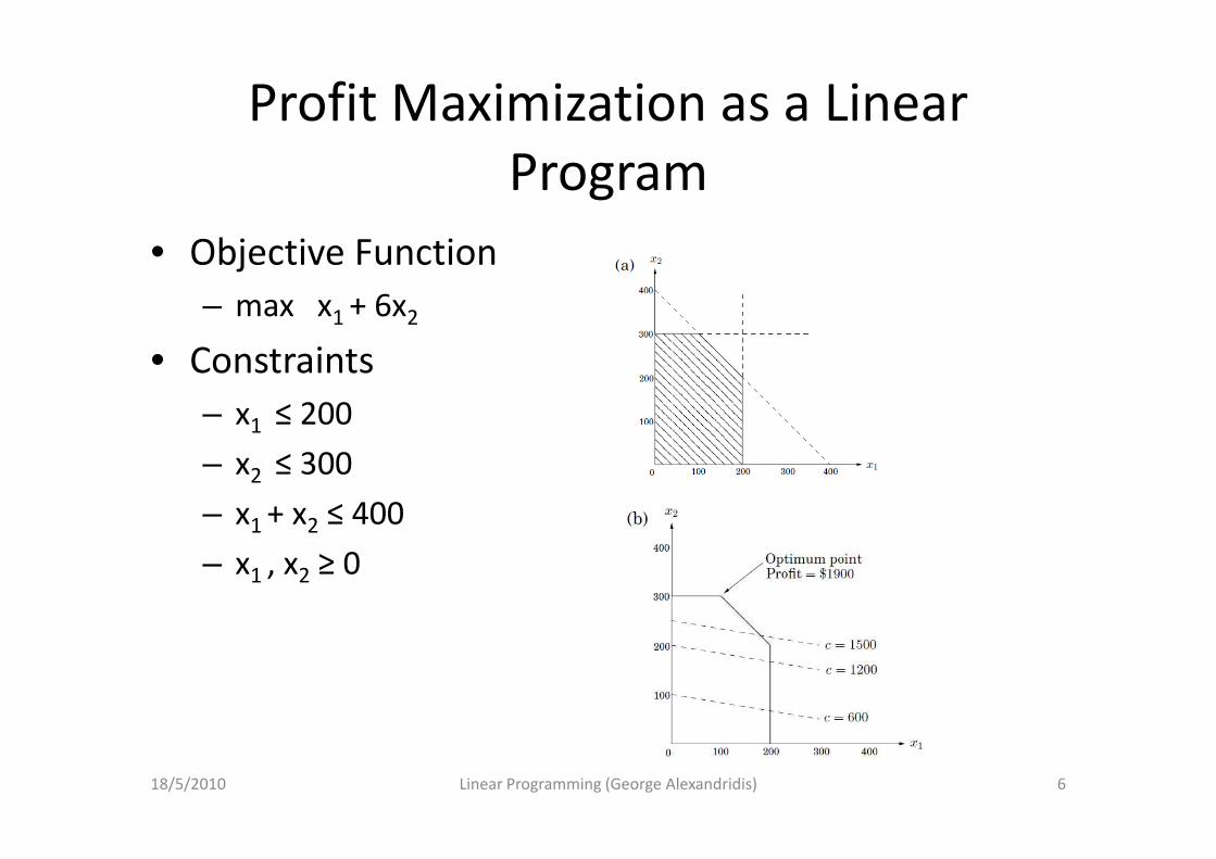
• Objective Function

– max x1 + 6x2

• Constraints

– x1 ≤ 200– x1 ≤ 200

– x2 ≤ 300

– x1 + x2 ≤ 400

– x1 , x2 ≥ 0


The simplex algorithm

• Let v be any vertex of

the feasible region

• While there is a

neighbor v’ of v with neighbor v’ of v with

better objective value:

– Set v = v’

• This local test implies

global optimality


Introduction to Duality

• Simplex outputs (x1, x2) = (100, 300) as the optimum solution, with an objective value of 1900. Can this answer be verified?– Multiply the second inequality by six and add it to the first

inequality• x1 + 6x2 ≤ 2000• x1 + 6x2 ≤ 2000

• The objective function cannot have a value of more than 2000!

– An even lower bound can be achieved if the second inequality is multiplied by 5 and then added to the third

• x1 + 6x2 ≤ 1900

– Therefore, the multipliers (0, 5, 1) constitute a certificate of optimality for our solution!

• Do such certificates exist for other LP programs as well?– If they do, is there any systematic way of obtaining them?


The Dual• Let’s define the multipliers y1, y2, y3 for the three constraints of our

problem– They must be non-negative in order to maintain the direction of the

inequalities

– After the multiplication and the addition steps, the following bound is obtained

• (y1 + y3)x1 + (y2 + y3)x2 ≤ 200y1 + 300y2 + 400y3

– The left hand-side of the inequality must resemble the objective function. Thereforefunction. Therefore

• x1 + 6x2 ≤ 200y1 + 300y2 + 400y3, if– y1, y2, y3 ≥ 0

– y1 + y3 ≥ 1

– y2 + y3 ≥ 6

• Finding the set of multipliers that give the best upper bound on the original LP is equivalent to solving a new LP!– min 200y1 + 300y2 + 400y3, subject to

– y1, y2, y3 ≥ 0

– y1 + y3 ≥ 1

– y2 + y3 ≥ 6


Primal – Dual

• Any feasible value of this dual LP is an upper

bound on the original primal LP (the reverse

also holds)

– If a pair of primal and dual feasible values are – If a pair of primal and dual feasible values are

equal, then they are both optimal

– In our example both (x1, x2) = (100, 300) and (y1,

y2, y3) = (0, 5, 1) have value 1900 and therefore

certify each other’s optimality


Formal Definition of the Primal and

Dual Problem

Here, the primal problem is a minimization problem.


LP Duality Theorem

• The LP-duality is a min-max relation

• Corollary 1 – LP is well – characterized

• Corollary 2– LP is in NP ∩ co-NP

– Feasible solutions to the primal (dual) provide Yes (No) certificates to the question:

• “Is the optimum value less than or equal to α?”


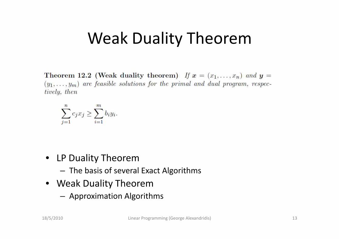
Weak Duality Theorem

• LP Duality Theorem

– The basis of several Exact Algorithms

• Weak Duality Theorem

– Approximation Algorithms


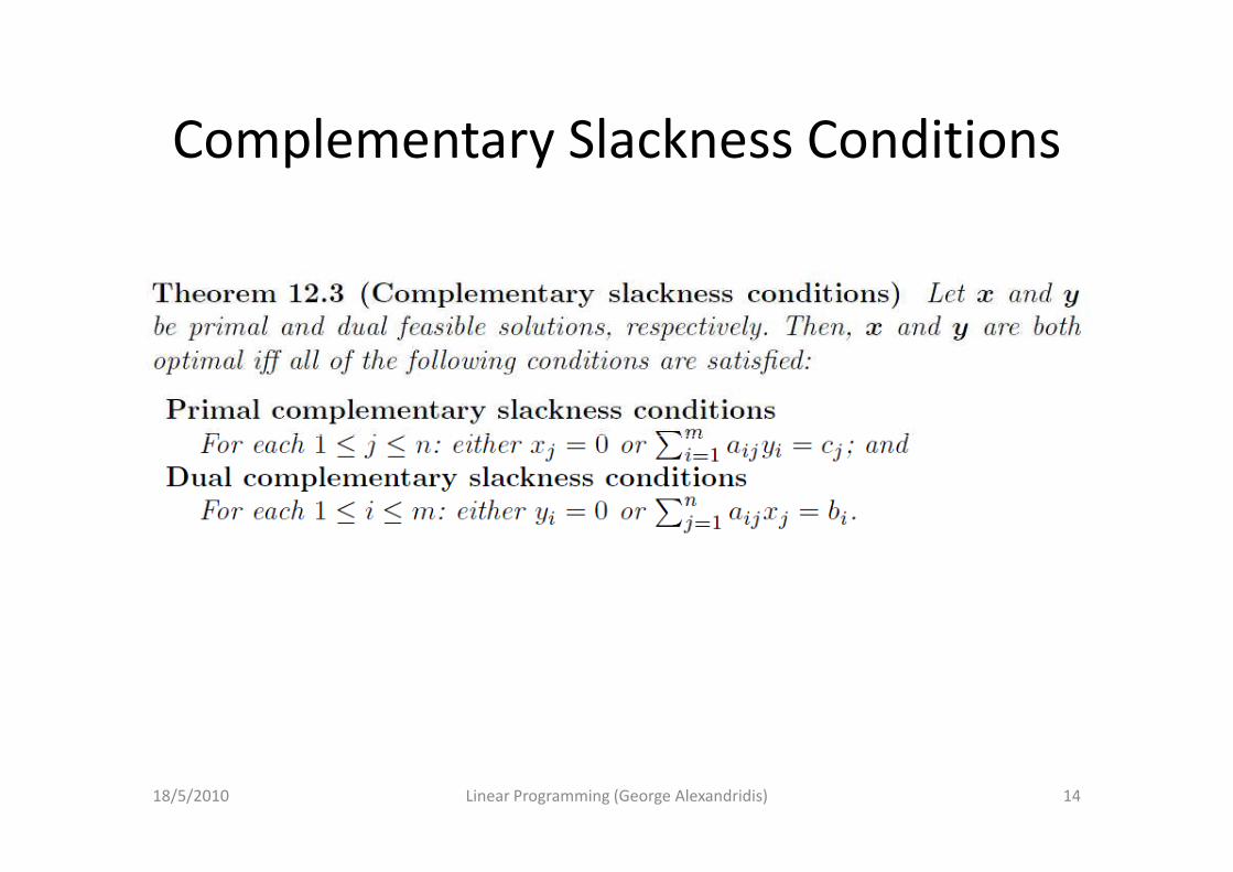
Complementary Slackness Conditions


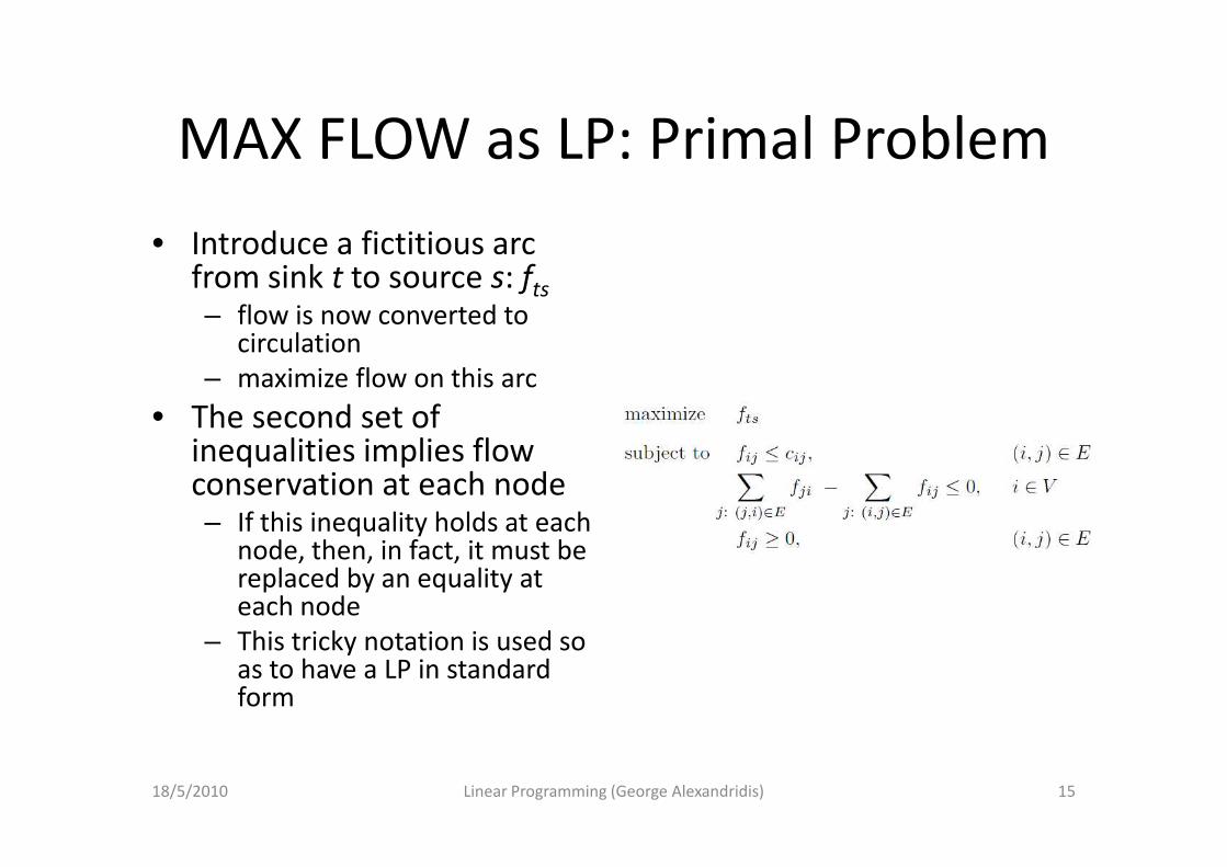
MAX FLOW as LP: Primal Problem

• Introduce a fictitious arc from sink t to source s: fts

– flow is now converted to circulation

– maximize flow on this arc

• The second set of inequalities implies flow

• The second set of inequalities implies flow conservation at each node– If this inequality holds at each

node, then, in fact, it must be replaced by an equality at each node

– This tricky notation is used so as to have a LP in standard form


MAX FLOW as LP: Dual Problem

• The variables dij and pi

correspond to the two

types of inequalities in

the primal

d : distance labels on – dij: distance labels on

arcs

– pi: potentials on nodes


MAX FLOW as LP: Transformation of

the Dual to an Integer Program• The integer program seeks 0/1

solutions

• If (d*,p*) is an optimal solution to IP, then the 2nd inequality is satisfied only if ps

* = 1 and pt* = 0, thus

defining an s-t cut– S is the set of potential 1 nodes and V /

S the set of potential 0 nodesS the set of potential 0 nodes

• If the nodes of an arc belong to the different sets ( ), then by the first inequality dij

* = 1

• The distance label for each of the remaining arcs may be set to 0 or 1 without violation of the constraint

– it will be set to 0 in order to minimize the objective function

• Therefore the objective function will be equal to the capacity of the cut, thus defining a minimum s-t cut


MAX FLOW as LP: LP-relaxation

• The previous IP is a formulation of the minimum s-t cut problem!

• The dual program may be seen as a relaxation of the IP– the integrality constraint is dropped

– 1 ≥ dij ≥ 0, for every arc of the graph

– 1 ≥ pi ≥ 0, for every node of the graph

– the upper bound constraints on the variables are redundant– the upper bound constraints on the variables are redundant• Their omission cannot give a better solution

• The dual program is said to be an LP-Relaxation of the IP

• Any feasible solution to the dual problem is considered to be a fractional s-t cut– Indeed, the distance labels on any s-t path add up to at least 1

• The capacity of the fractional s-t cut is then defined to be the dual objective function value achieved by it


The max-flow min-cut theorem as a

special case of LP-Duality• A polyhedron defines the set of feasible solutions to the

dual program– A feasible solution is set to be an extreme point solution if it is a

vertex of the polyhedron• It cannot be expressed as a convex combination of two feasible

solutions

– LP theory: there is an extreme point solution that is optimal– LP theory: there is an extreme point solution that is optimal

• It can be further proven that each extreme point solution of the polyhedron is integral with each coordinate being 0 or 1

• The dual problem has always an integral optimal solution

• By the LP duality theory, maximum flow in G must equal the capacity of a minimum fractional s-t cut– Since the latter equals the capacity of a minimum s-t cut, we get

the max-flow min-cut theorem


Another consequence of the LP-

Duality Theorem: The Farkas’ Lemma• Ax = b, x ≥ 0 has a solution iff there is no vector y ≠ 0 saTsfying ATy ≤ 0 and bTy > 0

• Primal: min 0Tx– Ax = b

– x ≥ 0

• Dual: max bTy– ATy ≤ 0

– y ≠ 0

• If the primal is feasible, it has an optimal point of cost 0• If the primal is feasible, it has an optimal point of cost 0– y = 0 is feasible in the dual and therefore it is either unbounded or has an optimal point

• First direction– If Ax = b has an non-negative solution, then the primal is feasible and its optimal cost is 0.

Therefore, the dual’s optimal cost is 0 and there can be no vector y satisfying the dual’s first constraint and bTy > 0

• Second direction– If there is no vector y satisfying ATy ≤ 0 and bTy > 0, then the dual is not unbounded. It has an

optimal point. As a consequence the primal has an optimal point and therefore it is feasible


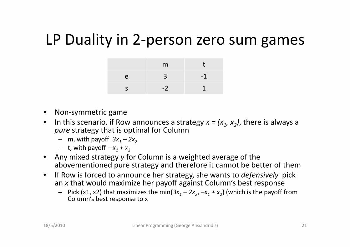
LP Duality in 2-person zero sum games

• Non-symmetric game

• In this scenario, if Row announces a strategy x = (x1, x2), there is always a

m t

e 3 -1

s -2 1

• In this scenario, if Row announces a strategy x = (x1, x2), there is always a pure strategy that is optimal for Column– m, with payoff 3x1 – 2x2

– t, with payoff –x1 + x2

• Any mixed strategy y for Column is a weighted average of the abovementioned pure strategy and therefore it cannot be better of them

• If Row is forced to announce her strategy, she wants to defensively pick an x that would maximize her payoff against Column’s best response– Pick (x1, x2) that maximizes the min{3x1 – 2x2, –x1 + x2} (which is the payoff from

Column’s best response to x

18/5/2010 Linear Programming (George Alexandridis) 21

LP of the 2-person zero sum game

• If Row, announces her strategy first, she needs to pick x1 and x2so that– z = min{3x1 – 2x2, –x1 + x2}

– max z• z ≤ 3x1 – 2x2

• z ≤ –x1 + x2

• In LP form

• If Column, announces his strategy first, he needs to pick y1 and y2 so that– w = max{3y1 – y2, –2y1 + y2}

– min w• w ≥ 3y1 – y2

• w ≥ –2y1 + y2

• In LP form• In LP form• max z

• x1 – 2x2 + z ≤ 0

• x1 – x2 + z ≤ 0

• x1 + x2 = 1

• x1, x2 ≥ 0

• In LP form• min w

• 3y1 – y2 + w ≥ 0

• -2y1 + y2 + w ≥ 0

• y1 + y2 = 1

• y1, y2 ≥ 0


These two LPs are dual to each other

They have the same optimum V

The min-max theorem of game theory

• By solving an LP, the maximizer (Row) can determine a strategy for herself that guarantees an expected outcome of at least V no matter what Column does– The minimizer, by solving the dual LP, can guarantee an

expected outcome of at most V, no matter what Row does

• This is the uniquely defined optimal play and V is the value• This is the uniquely defined optimal play and V is the valueof the game– It wasn’t a priori certain that such a play existed

• This example cat be generalized to arbitrary games– It proves the existence of mixed strategies that are optimal for

both players

– Both players achieve the same value V

– This is the min-max theorem of game theory


Linear Programming in Approximation

Algorithms• Many combinatorial optimization problems can be stated

as integer problems– The linear relaxation of this program then provides a lower

bound on the cost of the optimal solution

– In NP-hard problems, the polyhedron defining the optimal solution does not have integer verticessolution does not have integer vertices

• In that case a near-optimal solution is sought

– Two basic techniques for obtaining approximation algorithms using LP

• LP-rounding

• Primal-Dual Schema

– LP-duality theory has been used in combinatorially obtained approximation algorithms

• Method of dual fitting (Chapter 13)


LP-Rounding and Primal-Dual Schema

• LP-Rounding– Solve the LP

– Convert the fractional solution obtained into an integral solution• Ensuring in the process that the cost does not increase much

• Primal-Dual Schema– Use the dual of the LP-relaxation (in which case becomes the – Use the dual of the LP-relaxation (in which case becomes the

primal) in the design of the algorithm

– An integral solution to the primal and a feasible solution to the duela are constructed iteratively

– Any feasible solution to the dual provides a lower bound for OPT

• These techniques are illustrated in the case of SET COVER, in Chapter 14 and 15 of the book


The integrality gap of an LP-relaxation

• Given an LP-relaxation of a minimization problem Π, let OPTf(I) be the optimal fractional solution to instance I

• The integrality gap is then defined to be

– The supremum of the ratio of the optimal integral and fractional solutionsfractional solutions

– In case of a maximization problem, it would have been the infimum of this ratio

• If the cost of the solution found by the algorithm is compared directly with the cost of an optimal fractional solution, then the best approximation factor is the integrality gap of the relaxation


Running times of the two techniques

• LP-rounding needs to find an optimal solution to the linear programming relaxation– LP is in P and therefore this can be done in polynomial time if

the relaxation has polynomially many constraints.

– Even if the relaxation has exponentially many constraints, it may still be solved in polynomial time if a polynomial time separation oracle can be constructedstill be solved in polynomial time if a polynomial time separation oracle can be constructed

• A polynomial time algorithm that given a point in Rn (n: the number of variables in the relaxation) either confirms that it is a feasible solution or outputs a violated constraint.

• The primal-dual schema may exploit the special combinatorial structure of individual problems and is able to yield algorithms having good running times– Once a basic problem is solved, variants and generalizations of

the basic problem can be solved too


LINEAR PROGRAMMING - Corelab said to be a feasible solution 18/5/2010 Linear Programming ... the...

Documents

Transcript of LINEAR PROGRAMMING - Corelab said to be a feasible solution 18/5/2010 Linear Programming ... the...