
Linear Programming
18
Linear Programming Linear Programming Excel Solver
-
Upload
orlando-farrell -
Category
Documents
-
view
17 -
download
3
description
Linear Programming. Excel Solver. The Linear Programming Model. MAX8X 1 + 5X 2 s.t.2X 1 + 1X 2 ≤ 1000 (Plastic) 3X 1 + 4X 2 ≤ 2400 (Prod. Time) X 1 + X 2 ≤ 700 (Total Prod.) X 1 - X 2 ≤ 350 (Mix) All x’s ≥ 0. - PowerPoint PPT Presentation
Transcript of Linear Programming

Linear ProgrammingLinear Programming
Excel Solver
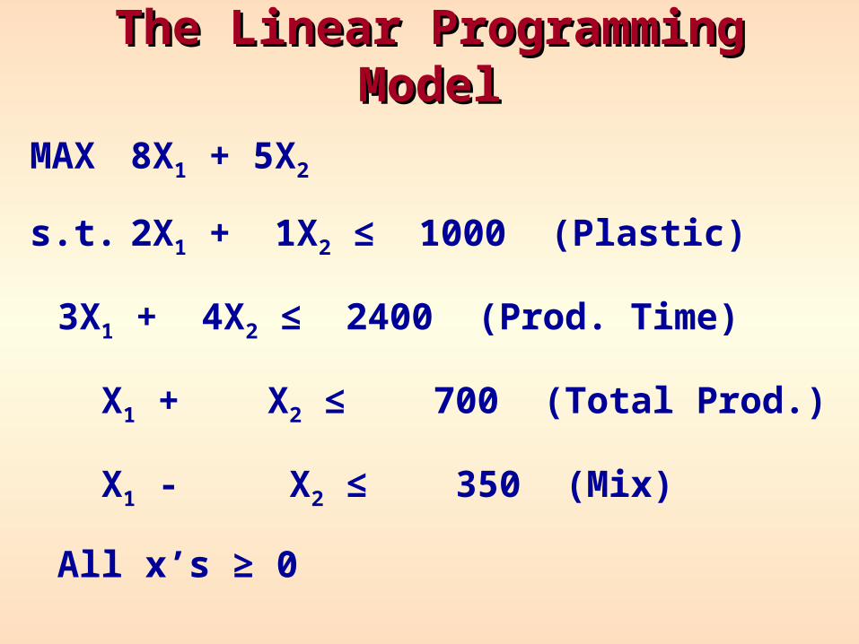
MAX 8X1 + 5X2
s.t. 2X1 + 1X2 ≤ 1000 (Plastic)
3X1 + 4X2 ≤ 2400 (Prod. Time)
X1 + X2 ≤ 700 (Total Prod.)
X1 - X2 ≤ 350 (Mix)
All x’s ≥ 0
The Linear Programming ModelThe Linear Programming Model
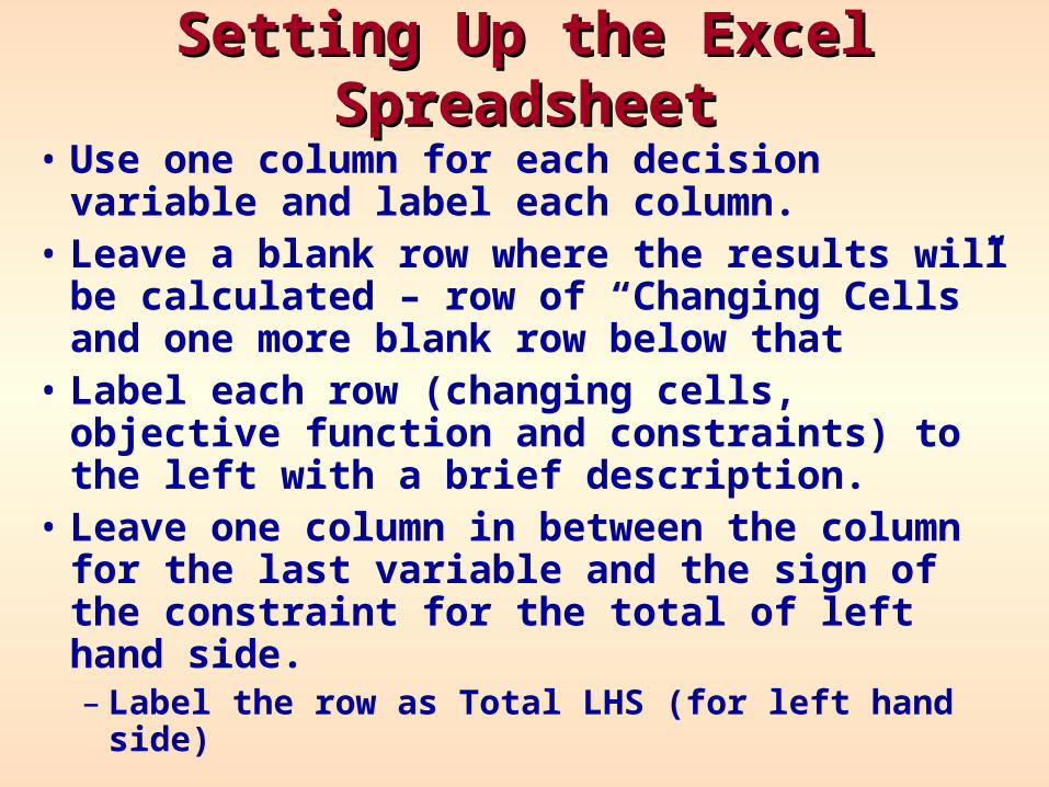
Setting Up the Excel SpreadsheetSetting Up the Excel Spreadsheet
• Use one column for each decision variable and label each column.
• Leave a blank row where the results will be calculated – row of “Changing Cells” and one more blank row below that
• Label each row (changing cells, objective function and constraints) to the left with a brief description.
• Leave one column in between the column for the last variable and the sign of the constraint for the total of left hand side.– Label the row as Total LHS (for left hand side)

Input Coefficients/ Label RowsInput Coefficients/ Label RowsChanging Cells Label Changing Cells
Where results will be given
ConstraintLabels
Label forLeft Hand Side Total
CoefficientsObjective FunctionLabel

Enter SUMPRODUCT Formula for Enter SUMPRODUCT Formula for the Total Proiftthe Total Proift
=SUMPRODUCT($C$4:$D$4,C6:D6)is equivalent to
=$C$4*C6+$D$4*D6
Highlight cells C4 and D4and press the F4 function
key to enter $ signs
Highlight cellsC6 and D6
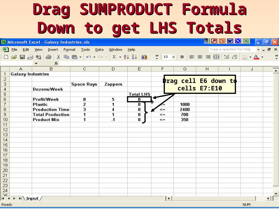
Drag SUMPRODUCT FormulaDrag SUMPRODUCT FormulaDown to get LHS TotalsDown to get LHS Totals
+
Drag cell E6 down tocells E7:E10
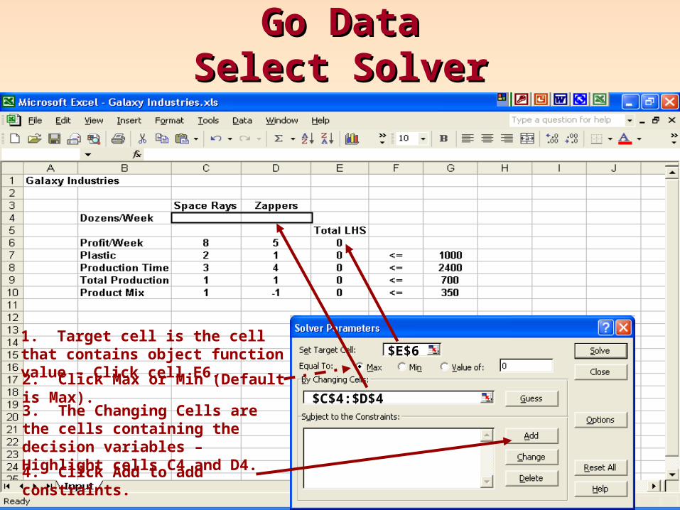
Go DataGo DataSelect SolverSelect Solver
$E$61. Target cell is the cell that contains object function value – Click cell E6.
2. Click Max or Min (Default is Max).
3. The Changing Cells are the cells containing the decision variables – Highlight cells C4 and D4.
$C$4:$D$4
4. Click Add to add constraints.
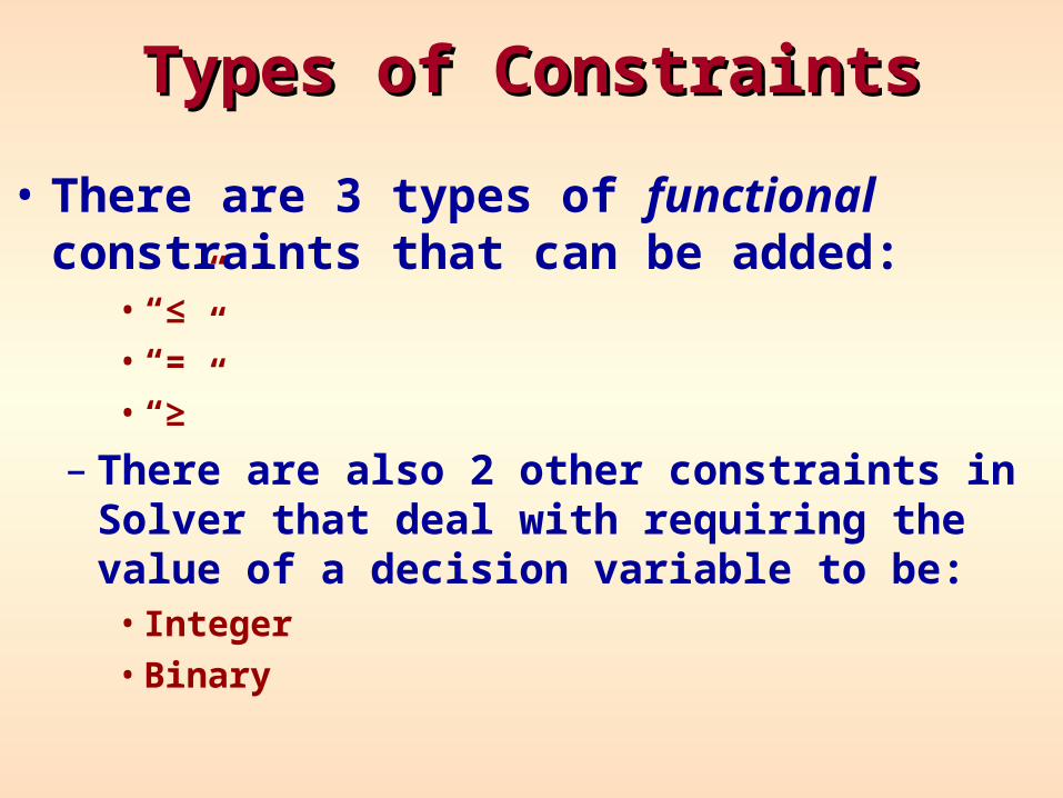
Types of ConstraintsTypes of Constraints
• There are 3 types of functional constraints that can be added:
• “≤”• “=”• “≥”
– There are also 2 other constraints in Solver that deal with requiring the value of a decision variable to be:
• Integer• Binary

Adding A Functional ConstraintAdding A Functional Constraint• The general approach is:
≤=≥
Click on a cell reference containing
a total LHS value
$E$7
Click on the cell reference containing the
corresponding RHS value
$G$7
Click Add if more constraints are to
be entered
Click OK if no more constraints are to be entered
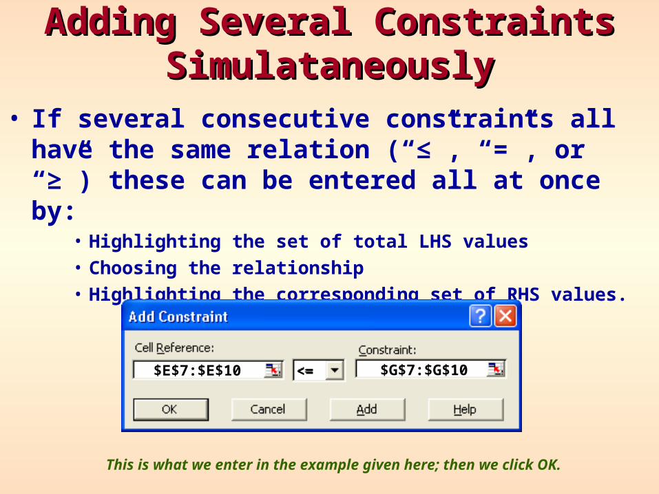
Adding Several Constraints Adding Several Constraints SimulataneouslySimulataneously
• If several consecutive constraints all have the same relation (“≤”, “=”, or “≥”) these can be entered all at once by:
• Highlighting the set of total LHS values• Choosing the relationship• Highlighting the corresponding set of RHS values.
$E$7:$E$10 $G$7:$G$10<=
This is what we enter in the example given here; then we click OK.
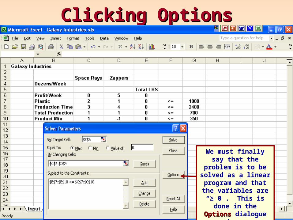
Clicking OptionsClicking Options
We must finally say that the problem is to be solved as a linear program and that the variables are “≥ 0”. This is done in the
OptionsOptions dialogue box.
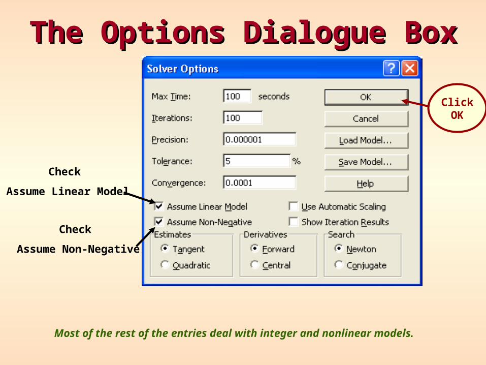
The Options Dialogue BoxThe Options Dialogue Box
Check
Assume Linear Model
Check
Assume Non-Negative
Most of the rest of the entries deal with integer and nonlinear models.
ClickOK

Click SolveClick Solve
ClickSolve
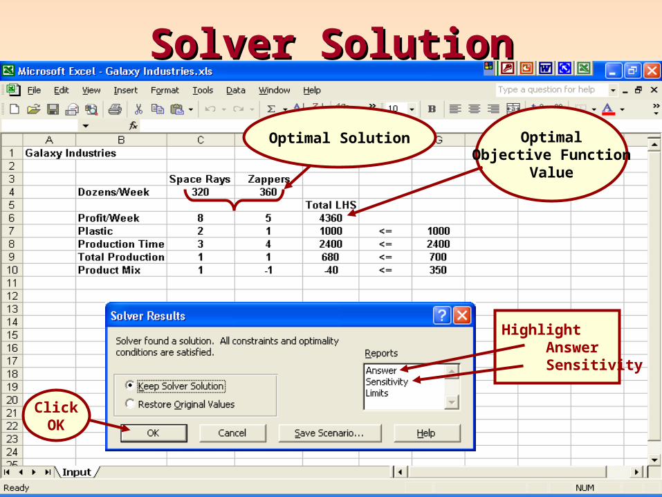
Solver SolutionSolver Solution
Optimal Solution OptimalObjective Function
Value
Highlight Answer Sensitivity
ClickOK
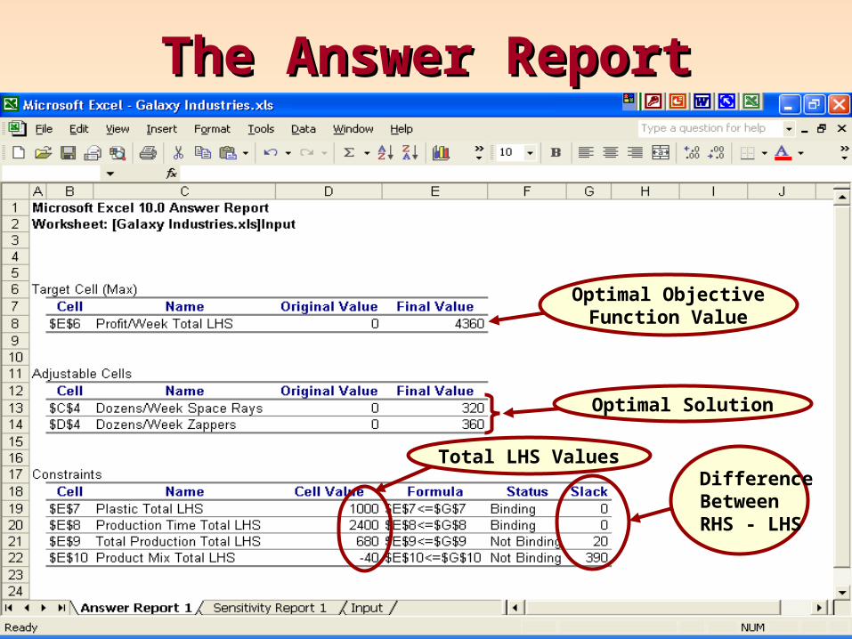
The Answer ReportThe Answer Report
Optimal ObjectiveFunction Value
Optimal Solution
Total LHS ValuesDifferenceBetweenRHS - LHS
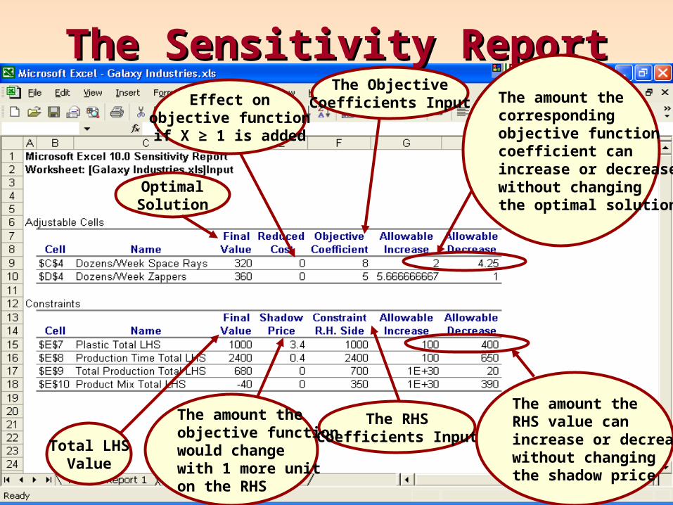
The Sensitivity ReportThe Sensitivity Report
OptimalSolution
The ObjectiveCoefficients Input
The RHSCoefficients Input
The amount thecorrespondingobjective functioncoefficient canincrease or decreasewithout changingthe optimal solution
The amount theRHS value canincrease or decreasewithout changingthe shadow price
Total LHSValue
The amount theobjective functionwould changewith 1 more uniton the RHS
Effect onobjective functionif X ≥ 1 is added
Notes on Sensitivity Report OutputNotes on Sensitivity Report Output• 1E+30 is Excel’s way of saying “infinity”
• Allowable Increases and Decreases apply to changing that one coefficient only – keeping all of the other coefficients the same.
• Reduced Cost has many meanings:– How would the objective function be affected if
the variable had to assume a value of at least 1– How much would the objective function
coefficient have to change before it is economically beneficial for the corresponding variable to be positive.
ReviewReview
• How to set up an Excel spreadsheet to solve a linear program
• Filling in the Solver dialogue box.
• How to “Add Constraints”
• Filling in the Options dialogue box
• Reading and interpreting:– Excel Output– The Answer Report– The Sensitivity Report


