Linear Parameter-Varying Modelling and Robust Control of ...
188
Linear Parameter-Varying Modelling and Robust Control of Variable Cam Timing Engines Ali Umut Gen¸c Wolfson College Cambridge A dissertation submitted to the University of Cambridge for the degree of Doctor of Philosophy November 2002
Transcript of Linear Parameter-Varying Modelling and Robust Control of ...

Linear Parameter-Varying Modelling
and Robust Control
of Variable Cam Timing Engines
Ali Umut Genc
Wolfson CollegeCambridge
A dissertation submitted to theUniversity of Cambridge for
the degree of Doctor of Philosophy
November 2002

In memory of my father
Ismail Hakkı Genc
c© 2002 Ali Umut Genc
Hopkinson LabDepartment of EngineeringTrumpington StreetCambridge CB2 1PZUnited Kingdom

Abstract
In this thesis the air-fuel ratio (AFR) control problem is investigated for a gasoline, portfuel injected, twin-independent variable cam timing engine. A complete parameter-varyingAFR path model is proposed and identified. In order to separate the effects of the fueland air on the measured AFR, gaseous fuel experiments are performed as well as gasolineones. It is shown that variable cam timing not only alters the air flow into the cylindersbut also the fuel flow. A reliable cylinder air charge model that can predict the transientbehaviour of the air charge entering the cylinder is identified with the help of the gaseousfuel experiments. Moreover, a global nonlinear identification scheme is proposed andsuccessfully implemented to identify the wall-wetting dynamics modelled as a slow and afast fuel puddle. The resulting parameter-varying model is able to predict the observedAFR transients induced by variable cam timing very accurately.
The second half of the thesis reviews the linear parameter-varying (LPV) controllerdesign techniques in the context of H∞ loop shaping controller design, which is the maincontroller synthesis paradigm in this thesis. The identified AFR model can be approxi-mated with a linear fractional transformation (LFT) model varying with manifold pressureand valve timings. The LFT AFR path model allows the use of any LPV controller designtechnique for AFR controller synthesis. Experimental evaluation of the designed LTI andLPV H∞ loop shaping AFR controllers reveals that the LPV controller offers up to 50 %improvements in AFR regulation performance without any feedforward action. Furtherimprovements in performance are obtained by introducing feedforward elements into thecontrollers. The testing of the final controllers under various conditions including rapidtransients has revealed that when coupled with a well designed feedforward controller boththe LPV and LTI controllers perform equally well.
Keywords: Variable cam timing engines, air-fuel ratio control, gaseous fuel, wall-wetting,
i

ii
H∞ loop shaping, LPV control, LFT systems, gain scheduling, nonlinear identification,robust control.

Preface
It has been four years and few months since I had been to Cambridge for the first timefor an interview with Keith and Nick on a sunny August day. My Ph.D. ”adventure” hasbeen a great experience and challenge. As with any adventure I have made many friendson the way and they all in one way or the other contributed to this piece. I would like totake this opportunity to acknowledge the help and support of the few.
Firstly, I would like to express my gratitude to my supervisor, Professor Keith Gloverwho not only guided me throughout this research but also provided reassurance duringdifficult times.
Professor Nick Collings has been an excellent adviser and a creative experimentalist;propane experiments wouldn’t have taken place without his lead. Special thanks should goto Dr. Richard Ford who had been an excellent R.A. and a friend. He helped me with bothengine testing and related control issues. Performing engine tests on a daily basis wouldn’tbe possible without the excellent support of technicians in the department. Particularthanks to Dave Gautrey, John Harvey, Trevor Parsons and Michael Underwood. Thecustom soft and hardware for engine control was developed at the Advanced PowertrainGroup Ford Motor Co. Special thanks to Julian Hodgson for the technical support duringthe commissioning of the VCT engine.
Thanks to Merten Jung, Christos Papageorgiou, George Biskos, Dr. Eric Kerrigan, Dr.Kelvin Halsey, and Dr. Rahmi Oklu who helped me proof read this thesis; the number oftypos and missing ”the”s have been significantly reduced. My co-workers and the facultyin the control and engines-emissions-control groups deserve a mention since they havealways been friendly and helpful: thank you all. Special thanks to Dr. Michael Cantoniand Dr. George Papageorgiou who were always willing to help me with any problem.
The area of this study was proposed by Mr. Derek Eade and Mr. Andy Scarisbrick ofFord Motor Co. whose generous funds financed my Ph.D. and together with the Engineer-
iii
iv
ing and Physical Sciences Research Council (EPSRC) financed the engine test facilities. Iam very grateful for their support.
I have had many good friends in Cambridge who made my stay richer and more fun.I will miss for sure never-ending discussions with Dr. Polykarpos Papadopoulos, damnfunny ”geyik”s with Abdulkadir Hallac, and the all-is-perfect attitude of Merten Jung. Ialso enjoyed and had great fun (and always lost) on each ”rgf” poker club night.
My mum does not speak English so, ”Bana hep destek ve sevgi veren anneme, aramızdanzamansız ayrılan babama ve cılgın kızkardesime beni hic bir zaman yalnız bırakmadıklarıicin minnettarım”. Finally, Dicle Kortantamer has been great company during the goodand bad times; without her support it would have been too difficult.
A. Umut GencCambridge, November 2002
As required by University Statute, I hereby declare that this dissertation is the resultof my own work and includes nothing which is the outcome of work done in collaborationexcept where specifically indicated in the text.
This dissertation contains no more than 65,000 words and 150 figures.
Contents
Abstract i
Preface iii
List of Figures ix
List of Tables xiii
Notation and Acronyms xv
1 Introduction 1
1.1 Gasoline Engines 21.2 Air-Fuel Ratio Control 31.3 Variable Cam Timing 6
1.3.1 Control Issues in VCT engines 91.4 Thesis Layout 11
2 Transient VCT Disturbances on AFR 13
2.1 Gasoline Experiments 132.2 Propane Experiments 162.3 Comments 20
3 Modelling and Identification of the AFR Path 21
3.1 Air Path Dynamics 233.1.1 Throttle Mass Air Flow 233.1.2 Cylinder Mass Air Flow 263.1.3 Intake Manifold Model 31
v
vi Table of Contents
3.2 Fuel Path Dynamics 343.2.1 Model Structure 36
3.2.2 Local Linear or Global Identification 413.2.3 Delay, Gas Mixing and Sensor Dynamics 43
3.2.4 Injector Calibration 473.2.5 Wall-Wetting Dynamics 48
3.3 Transient Validation of the AFR Model 60
3.4 Comments 63
4 LFT Representation of the AFR Path Model 67
4.1 Injection Delay 694.2 Wall-Wetting Dynamics 70
4.3 Transport Delay 714.4 Gas Mixing and Sensor Dynamics 73
4.5 Cylinder Mass Air Flow 74
4.6 Overall AFR Path 754.7 Comments 76
5 Robust Control System Design 77
5.1 Typical Closed-Loop Requirements 78
5.2 H∞ Control with Linear Matrix Inequalities 825.2.1 Synthesis LMIs 85
5.2.2 Example: LTI H∞ Loop Shaping Controller Design 89
5.3 Gain-scheduling and LPV Systems 915.3.1 General Parameter Dependence 94
5.3.2 Rational Parameter Dependence 955.3.3 LPV Controller Synthesis for General Parameter Dependence 98
5.3.4 LPV Controller Synthesis for Rational Parameter Dependence 1025.3.5 Example: LPV H∞ Loop Shaping Controller Design 110
5.4 Comments 112
6 AFR Control System Design 115
6.1 H∞ Loop Shaping Controller Design 116
6.1.1 LTI H∞ Loop Shaping Controller 1166.1.2 LPV H∞ Loop Shaping Controller 118
6.2 Controller Performance in Simulations 1226.3 Controller Performance in Experiments 124
6.3.1 Feedback Only 126

Table of Contents vii
6.3.2 Feedback-plus-Feedforward 1316.3.3 More Realistic Disturbance Scenarios 138
6.4 Comments 144
7 Conclusions 145
7.1 Main Contributions 1457.2 Further Work 146
A Facilities 149
A.1 Dynamometer 149A.2 Engine 149A.3 Software 150A.4 Actuators and Sensors 150
B Input Excitations for Linear Identification 153
B.1 PRBS 153B.2 Multi-Sine 154
C H∞ Loop Shaping 157
C.1 McFarlane and Glover’s Design Procedure 159C.2 ν-Gap Metric 160
Bibliography 161


List of Figures
1.1 Market share of diesel in Europe (Source: JD Power-LMC automotive) 21.2 Catalyst conversion efficiency for NOx, CO and HC [Hey88] 41.3 Closed-loop AFR control system 51.4 Toyota VCT Mechanism 7
2.1 Transient EVC disturbance on AFR (gasoline experiment) 142.2 Transient IVO disturbance on AFR (gasoline experiment) 152.3 Transient EVC disturbance on AFR signal (propane experiment) 172.4 Transient IVO disturbance on AFR signal (propane experiments) 18
2.5 Variations in the inlet port temperature at 40kPa under VCT excitation 19
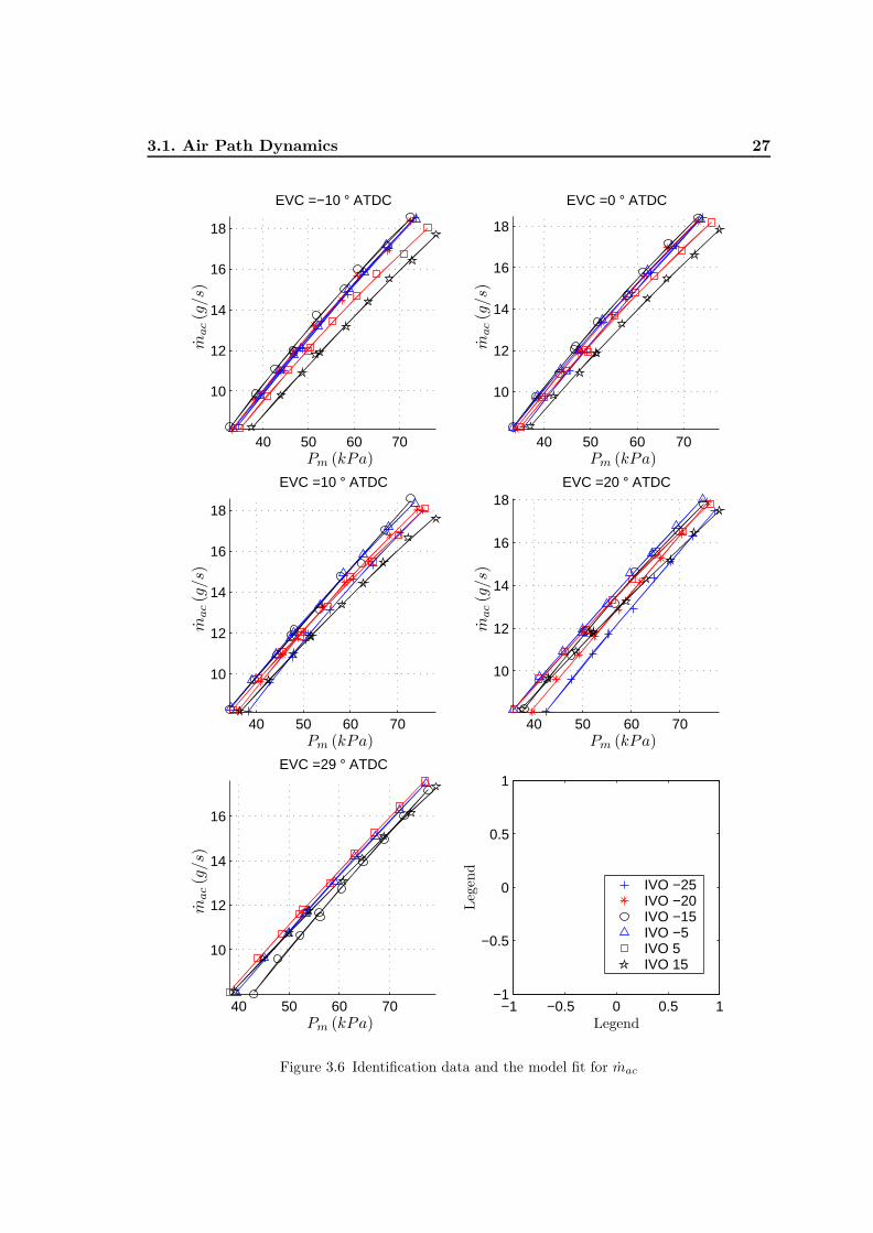
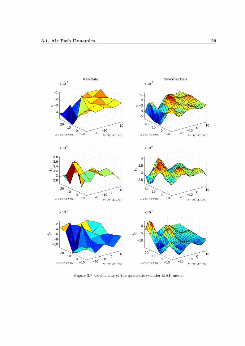
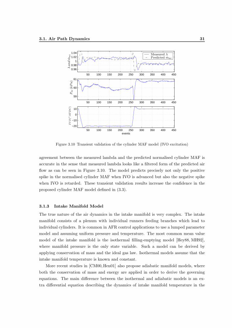
3.1 Main sensors used in the AFR path identification 223.2 A sample steady state engine test for IVO=5◦and EVC=29◦ 243.3 Steady state measurements of the throttle MAF and the model fit 253.4 Transient validation of the throttle MAF (EVC excitation) 253.5 Transient validation of the throttle MAF model (IVO excitation) 263.6 Identification data and the model fit for mac 273.7 Coefficients of the quadratic cylinder MAF model 293.8 Identified cylinder MAF surfaces 303.9 Transient validation of the cylinder MAF model (EVC excitation) 303.10 Transient validation of the cylinder MAF model (IVO excitation) 313.11 Transient validation of the intake MAP model (EVC excitation) 333.12 Transient validation of the intake MAP model (IVO excitation) 333.13 Transient validation of the intake MAP model (TP excitation) 343.14 Fuel path dynamics for one cylinder 353.15 Fuel path dynamics for a 4-cylinder engine 36
ix
x List of Figures
3.16 Normalised step responses of the fuel path 383.17 Identified frequency responses of the fuel path at different operating points 393.18 Measured lambda and predicted normalised cylinder MAF 403.19 Measured and predicted frequency responses at two different operating points 433.20 Measured and predicted time responses at two different operating points 443.21 Variation of the transport delay with valve overlap and manifold pressure 453.22 Variation of ξ1 with the valve overlap and manifold pressure 463.23 Variation of ξ2 with the valve overlap and manifold pressure 463.24 Injector calibration data 483.25 Global identification framework for wall-wetting dynamics 493.26 Global data for the identification of the wall-wetting dynamics 533.27 Measured and predicted trajectories of the dφ
dt and lambda 543.28 Identified trajectories of the fast fuel puddle parameters 553.29 Variation of Xf with the valve timings 573.30 Variation of τf with the valve timings 573.31 Variation of Xfτf during the identification experiment 583.32 Identified trajectories of the slow fuel puddle 583.33 Variation of Xs and τs with the manifold pressure 593.34 Zeros of Gww(z) 593.35 Transient validation of the AFR path model (EVC excitation) 613.36 Transient validation of the AFR path model (IVO excitation) 623.37 Transient validation of the AFR path model (FPW excitation) 64
4.1 Diagrammatic representations of Fl (P,Ql) and Fu (P,Qu) 684.2 Identified AFR path model 694.3 LFT representation of the wall-wetting dynamics 704.4 LFT representation of e−d
′s 734.5 LFT representation of the gas mixing and sensor dynamics 744.6 LFT approximation of m−1
acF 75
5.1 Interconnected system 795.2 Standard feedback configuration 805.3 Singular values of a typical loop shape 815.4 LFT control system synthesis framework 835.5 Singular values of nominal plant G0, weighted plant Gs and K∞Gs 905.6 H∞ loop shaping weights 915.7 Robust Stability margin for the frozen values of ρ 925.8 LFT control system synthesis framework 103

List of Figures xi
5.9 LTI robust stability margin for the frozen values of ρ 1135.10 Disturbance rejection performances of the H∞ loop shaping controllers 1135.11 Variation of the normalised scheduling parameter 114
6.1 Singular values of scaled nominal plant G0, weighted plant Gs and K∞Gs 1176.2 H∞ loop shaping weights 1186.3 Sample data for normalised Pm and Pm 1206.4 LTI robust stability margin for frozen values of Pm 1226.5 Performance of the controllers on the LFT model 1236.6 A realistic disturbance rejection test on the nonlinear model 1256.7 Aggressive TP disturbance rejection 1266.8 Moderate TP disturbance rejection 1286.9 EVC timing disturbance rejection 1296.10 IVO timing disturbance rejection 1306.11 Engine speed disturbance rejection 1326.12 Feedback-plus-Feedforward Control System Structure 1336.13 TP disturbance rejection (Feedback-plus-Feedforward) 1356.14 EVC disturbance rejection (Feedback-plus-Feedforward) 1366.15 IVO disturbance rejection (Feedback-plus-Feedforward) 1376.16 Engine speed disturbance rejection (Feedback-plus-Feedforward) 1396.17 A realistic disturbance rejection test (constant speed) 1416.18 A realistic disturbance rejection test (varying speed) 1426.19 Feedback and feedforward responses of the controllers 1436.20 Feedback responses of the controllers (zoomed) 143
A.1 Locations of the main sensors used in the AFR path identification 151
B.1 A PRBS signal with n = 7, 2n − 1 = 127, Tc = Ts = 4 154B.2 A multi-sine signal with Tmax = 684, Tmin = 9 and Ts = 1 155
C.1 The H∞ loop shaping typical block diagram 158C.2 Left coprime factor uncertain plant 158C.3 Interpretation of robust stability margin ε in the gap metric 160


List of Tables
3.1 Valve timings for the steady state identification experiments 233.2 Operating points of the fuel path identification experiments 373.3 Variation of the poles of Gx with the manifold pressure 473.4 Variation of the poles of Gx with the valve timings 47
5.1 Comparison of different LPV synthesis methods 111
6.1 Comparison of the LPV synthesis methods for AFR controller design 121
A.1 dSPACE boards 150A.2 Sensors in engine test cell 151
xiii


Notation and Acronyms
ENGINE
Acronyms
AFR Air-Fuel RatioATDC After Top Dead CentreBDC Bottom Dead CentreEGO Exhaust Gas OxygenEGR Exhaust Gas RecirculationEVC Exhaust Valve ClosingEVO Exhaust Valve OpeningFAR Fuel-Air RatioFPW Fuel Injection Pulse WidthIVC Inlet Valve ClosingIVO Inlet Valve OpeningMAF Mass Air FlowMAP Manifold Absolute PressureOCV Oil Control ValveOVL Valve OverlapPFI Port Fuel Injectionrpm Revolutions per MinuteSI Spark IgnitionTDC Top Dead CentreTI-VCT Twin Independent VCTTP Throttle PositionVCT Variable Cam Timing
xv
xvi Notation and Acronyms
VVT Variable Valve TimingWOT Wide Open Throttle
Symbols
mat Throttle MAFmac Cylinder MAFmfi Injected fuel massmfc Fuel mass sucked into cylindersmff Fuel film massτ Fuel film evaporation constantX Fuel film deposition constantPm MAPλ AFR relative to stoichiometricφ equivalence ratio, φ = λ−1
φc φ in cylinderφx φ in exhaustTs Sampling timeN Engine speed in rpm
CONTROL
Acronyms
LFT Linear Fractional TransformationLMI Linear Matrix InequalityLQG Linear Quadratic GaussianLTI Linear Time-InvariantLPV Linear Parameter-VaryingLTR Loop Transfer RecoveryMIMO Multiple Input Multiple OutputPI Proportional-IntegralPV Parameter-VaryingRHP Right Half PlaneSISO Single Input Single Output2DOF Two Degree-of-Fredoom
Fields of Numbers
R real numbers
Notation and Acronyms xvii
R+ strictly positive real numbersj the imaginary unit, i.e. j =
√−1
C complex numbersC+ open right-half plane
Relational Symbols
:= defined by≈ approximately equal to
Matrix Operations
0 zero matrix of compatible dimensionsI identity matrix of compatible dimensionsIn identity matrix of dimension n× n
A′ complex conjugate transpose of matrix AA−
′denotes
(A−1
)′ or equivalently (A′)−1
diag(A1, A2, . . . , An) block-diagonal matrix with matrices Ai on the main diagonalFl (P,Q) lower linear fractional transformation of matrices P and Q
Fu (P,Q) upper linear fractional transformation of matrices P and Q
A > 0 hermitian matrix A = A′ with strictly positive eigenvaluesA < 0 hermitian matrix A = A′ with strictly negative eigenvaluesA < B denotes (A−B) < 0
Function Spaces
L2 space of square integrable functions on jR including ∞H2 subspace of functions in L2 that are analytic in C+ and
uniformly square integrable along <(s) = α for all α ∈ R+
H∞ subspace of functions in L∞ that are analytic and bounded in C+
prefix R subspace of real-rational functions, e.g. RL2, RL∞
Measures of Size
σ(A) largest singular value of matrix Aσ(A) smallest singular value of matrix A|x| modulus (or magnitude) of x ∈ C‖x‖ Euclidean norm of x ∈ Cn
‖G‖2 two-norm of G ∈ RL2

xviii Notation and Acronyms
‖G‖∞ infinity-norm of G ∈ RL∞
Shorthand Notation(∗∗
)′(P + (∗) S
∗ R
)(T
V
)denotes the matrix
(T
V
)′(P + P ′ S
S′ R
)(T
V
)[A B
C D
]shorthand for state space realisation C (σI −A)−1 B +D,
σ = s, z
• do not care

1
Introduction
Automobile manufacturing is one of the biggest industries around the globe. Increas-ingly severe competition forces automobile manufacturers to reduce cost while at thesame time having to meet increasing tight, and therefore expensive emissions legislation.Coupled with this is a requirement, via pressures on CO2 reduction and customer needs,for improved quality in terms of fuel efficiency and vehicle safety. These objectives areinterrelated in fact usually conflicting. For example, lean-burn technology can improvefuel consumption significantly but at the same time it reduces the three-way catalystconversion efficiency. The opposing requirements of the modern automobiles can be metin different ways such as by improving the existing designs, by increased (mechanical)complexity or by introducing completely new designs. Hybrid engines, fuel cells, gasolinedirect injection and variable valve timing (VVT) are some of the new technologies avail-able today. However, since these innovations come with increased complexity they requiremore demanding control capability.
Variable cam timing (VCT) is one of these new technologies introduced recently inthe production engines. It offers the potential to achieve better fuel economy, emissionlevels and engine torque response. However, it can also cause a significant transient dis-turbance to the engine torque output adversely affecting driveability, and air-fuel ratio(AFR) degrading catalyst conversion efficiency. Thus, realising the full potential of theVCT engines requires a well-designed control system. This thesis investigates one par-ticular control problem in VCT engines: the so called AFR control problem. The mainobjectives of the thesis are threefold:
i. Propose and validate appropriate identification and modelling methods for the AFRpath in the VCT engines as an extension of the standard mean value engine models.
ii. Introduce and apply the recently developed linear parameter-varying controller de-
1
2 Introduction
sign methods to the AFR control problem in a unified and systematic framework.
iii. Encourage the use of the advanced robust control theory in real life control problems.
The AFR controller design problem investigated in this thesis focuses on the regulationof the AFR signal at the exhaust manifold i.e. before the catalyst under warm operatingconditions. Issues such as cold start emissions or regulation of the oxygen storage state ofthe catalyst in order to improve the emissions are not investigated in the thesis (althoughVCT has ability in this aspect). After a brief introduction to gasoline engines the rest ofthe chapter discusses the AFR control problem and VCT engines in detail.
1.1 Gasoline Engines
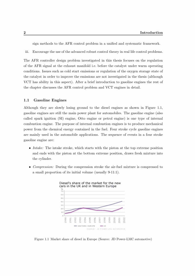
Although they are slowly losing ground to the diesel engines as shown in Figure 1.1,gasoline engines are still the main power plant for automobiles. The gasoline engine (alsocalled spark ignition (SI) engine, Otto engine or petrol engine) is one type of internalcombustion engine. The purpose of internal combustion engines is to produce mechanicalpower from the chemical energy contained in the fuel. Four stroke cycle gasoline enginesare mainly used in the automobile applications. The sequence of events in a four strokegasoline engine are:
• Intake: The intake stroke, which starts with the piston at the top extreme positionand ends with the piston at the bottom extreme position, draws fresh mixture intothe cylinder.
• Compression: During the compression stroke the air-fuel mixture is compressed toa small proportion of its initial volume (usually 9-11:1).
Figure 1.1 Market share of diesel in Europe (Source: JD Power-LMC automotive)

1.2. Air-Fuel Ratio Control 3
• Power (Expansion): During the power stroke, which starts with the piston near thetop (minimum volume) position and ends with the piston near the bottom (maximumvolume) position, the high pressure high temperature gases push down the pistonand do work on the rotating crank.
• Exhaust: Unburned and burned gases are expelled from the cylinder during theexhaust stroke.
In current gasoline engines fuel is injected into each inlet port near the inlet valve, whichis called port fuel injection (PFI), and the premixed charge is drawn into the cylindersand ignited. PFI gasoline engines have high power output, yet they suffer from lowercompression ratio, low thermal efficiency and high fuel consumption when compared withthe diesel or gasoline direct injection engines. The main causes of these drawbacks areknock and spontaneous ignition limits, high throttling and limited AFR operation range.The PFI gasoline engines run at stoichiometric AFR at most loads. A stoichiometric AFRdenotes a chemically correct proportion of air and fuel so that there is just enough oxygenfor conversion of all the fuel into completely oxidised products. For current gasoline fuel,the stoichiometric AFR by weight is approximately 14.6. A more useful measure is therelative AFR (or lambda),
λ =AFRactualAFRstoich
(1.1)
or its inverse the equivalence ratio (normalised fuel-air ratio (FAR))
φ = λ−1 =FARactualFARstoich
(1.2)
Then, a lean mixture gives λ > 1(φ < 1) and a rich mixture gives λ < 1(φ > 1).
1.2 Air-Fuel Ratio Control
In our ever-more-mobile society, reducing the vehicle pollution is an environmental im-perative. The tail pipe emissions contribute greatly to the air pollution and are alsothe primary cause of the air pollution in most urban areas. The main automotive airpollutants are carbon monoxide (CO), nitrogen oxides (NOx), hydrocarbons (HC), par-ticulates, and carbon dioxide (CO2). CO is a poisonous gas that displaces oxygen fromthe blood. At high concentrations it is fatal and at lower concentrations it can exacerbateheart problems. NOx react with HC in the sunlight to form ozone and photochemicalsmog. Moreover, it can increase respiratory illnesses and is a contributor to acid rain.Ozone causes breathing difficulties and damages plants due to its acidity. Diesel engines
4 Introduction
AFR window 14.4 14.5 14.6 14.7 14.8 14.9
20
40
60
80
Sto
ichi
omet
ric A
FR
Rich Lean
Cat
alys
t effi
cien
cy, %
Air−Fuel ratio
0.9863 0.9932 1.0068
100
1.01370.9795 1.02051
14.380% conversion
λ
NOx
HC
CO
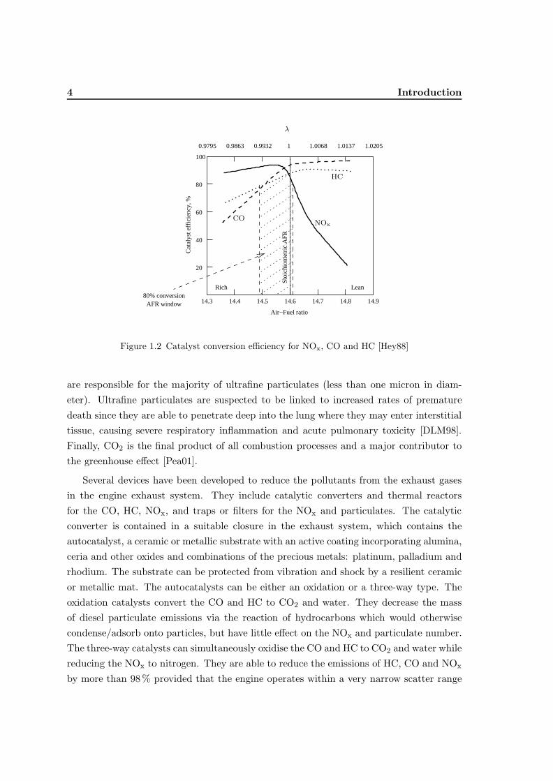
Figure 1.2 Catalyst conversion efficiency for NOx, CO and HC [Hey88]
are responsible for the majority of ultrafine particulates (less than one micron in diam-eter). Ultrafine particulates are suspected to be linked to increased rates of prematuredeath since they are able to penetrate deep into the lung where they may enter interstitialtissue, causing severe respiratory inflammation and acute pulmonary toxicity [DLM98].Finally, CO2 is the final product of all combustion processes and a major contributor tothe greenhouse effect [Pea01].
Several devices have been developed to reduce the pollutants from the exhaust gasesin the engine exhaust system. They include catalytic converters and thermal reactorsfor the CO, HC, NOx, and traps or filters for the NOx and particulates. The catalyticconverter is contained in a suitable closure in the exhaust system, which contains theautocatalyst, a ceramic or metallic substrate with an active coating incorporating alumina,ceria and other oxides and combinations of the precious metals: platinum, palladium andrhodium. The substrate can be protected from vibration and shock by a resilient ceramicor metallic mat. The autocatalysts can be either an oxidation or a three-way type. Theoxidation catalysts convert the CO and HC to CO2 and water. They decrease the massof diesel particulate emissions via the reaction of hydrocarbons which would otherwisecondense/adsorb onto particles, but have little effect on the NOx and particulate number.The three-way catalysts can simultaneously oxidise the CO and HC to CO2 and water whilereducing the NOx to nitrogen. They are able to reduce the emissions of HC, CO and NOx
by more than 98 % provided that the engine operates within a very narrow scatter range

1.2. Air-Fuel Ratio Control 5
controller
��������
air
fuel
catalyticconverter
tail−pipeemissions
fuel puddling
exhaust valve
throttlespark plug
intake valve
EGO sensor
Figure 1.3 Closed-loop AFR control system
(<1%) centred around the stoichiometric AFR (λ = 1) as depicted in Figure 1.2 [Bau99].Since maintaining the AFR in this restricted range under all operating conditions is avery difficult task for open loop fuel systems, closed-loop control of the AFR has beenintroduced. This system relies on a closed-loop control system to consistently maintainthe AFR mixture entering the engine within the optimal range known as the AFR window.An oxygen sensor (lambda sensor) in the exhaust system is used to monitor the AFR ofthe exhaust gas composition.
The AFR (lambda) closed-loop control systems incorporating a catalytic converter,such as the one depicted in Figure 1.3, are very effective in cleaning the exhaust gasesfrom the SI engines. The lambda sensor monitors the AFR composition in the exhaustand the amount of injected fuel is manipulated by the control system to maintain themeasured lambda at unity. The throttle is controlled by the driver in a conventional SIengine and constitutes the main disturbance on the AFR signal. The dynamic behaviourof the AFR system is also strongly affected by the fuel dynamics such as the fuel puddlein the inlet port. The fuel puddle dynamics describe the fact that even in a fully warmed-up engine a significant fraction of the fuel injected in each cycle impinges onto the inletport wall and valves, and enters the cylinder in subsequent cycles through evaporationand dribble. The delays in the AFR path such as the transport delay or injection delayput fundamental limitations on the achievable speed of response by a feedback controlsystem. This necessitates a feedforward element in the AFR control system in order toenhance the controller’s speed. Unfortunately, a feedforward controller has no robustnessagainst the uncertainty in the system and therefore requires high fidelity models to performsatisfactorily.
6 Introduction
Engine dynamics are nonlinear and operating point dependent. So-called mean valueengine models have been developed for the engine control system analysis and synthesispurposes [Dob80, Pow87, PC87, HS90, MH92, CM00]. These models are nonlinear in gen-eral. Usually linearised models are derived from the original nonlinear model at differentoperating points and linear control systems are designed for the linearised models. Al-though this approach has been shown to work in practice, further improvements in thefeedback controller performance can only be achieved if a nonlinear controller such as alinear parameter-varying controller is designed for the nonlinear engine model. A moredetailed discussion of the mean value engine models for the AFR control and the relatedliterature review will be presented in Chapter 3.
The classical approach to the AFR control is to design simple proportional-integral(PI) controllers at fixed operating points and to schedule the controller gains across theoperating envelope [Kie88]. Describing function analysis is used to analyse the limit cycleproperties caused by the sensor nonlinearities and time delays in the loop. The perfor-mance of this controller can be enhanced by introducing an open-loop control map (asimple feedforward element). Sliding mode feedback controllers have been developed asan alternative to the PI controllers [CH88]. The main advantage of these controllers isthat they have certain stability and robustness guarantees when state measurements areavailable. An LQG/LTR controller for combined AFR and engine speed control in a lim-ited speed range is published in [OG93]. Several other design methods are applied tothe AFR control problem such as feedback linearisation [BBC95,Guz95,XYM98] and H∞
loop shaping [Bra96].
However, engine control applications, including the AFR control, have been dominatedby observer based control systems. The main reason for using an observer/estimator isto improve the AFR regulation during transients by replacing the conventional empiricalfeedforward control with a model-based approach. The linear and nonlinear estimationtheories (such as Extended Kalman Filtering, adaptive observers) have applied to themean value models to get observers/estimators [PFC98, KRU98, CVH00]. Sliding modeobservers are developed in [CH98] as an extension of the sliding mode controllers.
The above short review of the AFR control is not exhaustive and a comprehensivereview can be found in [HL01].
1.3 Variable Cam Timing
Valves control the breathing of engines. The timing of the breathing, i.e. the timing of theair intake and exhaust, is controlled by the shape and phase angle of the cams. To optimisethe breathing whether from the point of view of volumetric efficiency, or emissions control,

1.3. Variable Cam Timing 7
Figure 1.4 Toyota VCT Mechanism
or combustion stability especially at cold start engines require different valve timings atdifferent conditions. In conventional SI engines the valve timing is, roughly speaking, atradeoff between the idle stability and wide-open-throttle (WOT) performance. Manyimprovements in engine operation in terms of idle quality, WOT performance, part-loademissions and fuel economy can be achieved, if the valve timings could be optimisedfor each engine speed and load. For example, the overlap between the intake strokeand exhaust stroke should be increased in order to improve performance as the manifoldpressure increases, i.e. wider throttle openings, and as the engine speed increases. Briefly,this is because the residual gases from the previous cycle will be more effectively removedwith increased overlap at these conditions.
VVT can be achieved in different ways [MWU+96]. The simplest mechanism calledVCT is depicted in Figure 1.4.1 The VCT alters the phase between the cam shaft and thecrankshaft. It consists of an oil control valve, a position sensor and the VCT pulley. Oilcontrol valve regulates the amount of oil pressure in the VCT pulley. This mechanism canmake the cam shaft retard/advance to any angle between the maximum limits. There are4 different types of VCT in double-over-head-cylinder engines:
• Intake Only (phasing only the intake cam);
• Exhaust Only (phasing only the exhaust cam);
• Twin Equal (phasing the intake and the exhaust cams equally);
1http://www.billzilla.org/vvtvtec.htm

8 Introduction
• Twin Independent (phasing the intake and the exhaust cams independently).
Twin independent (TI) VCT provides the most advantages among these at the cost ofincreased complexity. It can improve the part-load fuel consumption and emissions as wellas the idle quality, cold start emissions and WOT performance [LCS96]. In the followingsome advantages provided by TI-VCT are discussed in more detail.
Idle Quality
At idle the TI-VCT mechanism can be used to reduce or more correctly maintain a desiredquality of the residual gas fraction in the cylinder to maintain the idle stability. Toolittle residual gas has a detrimental effect on NOx production, and a limited amounthas virtually no effect on stability. In fact during warm-up, a certain quantity of hotresiduals is beneficial from the point view of encouraging fuel evaporation. As notedabove, in a fixed valve timing engine the amount of overlap at idle is a trade-off betweenthe idle quality and high speed power. The TI-VCT can reduce the valve overlap whenrequired without compromising high speed power. The improved idle quality from reducedoverlap could allow the engine to operate at lower idle speeds without losing stability. Forexample, [Ma88] shows that a 200 rpm reduction in idle speed from 800 rpm translates to6.1% improvement in the fuel consumption.
Part-load Emissions
Increasing the valve overlap at part-load increases the amount of residual gas trapped inthe cylinder. This functions as an internal exhaust gas recirculation (EGR) mechanismand reduces HC as well as the NOx emissions. The NOx reduction is due to the reducedcombustion temperatures but HC reduction mainly results from another opportunity toburn unburnt HC from the previous cycle. The same level of reduction of the HC emissionscannot be achieved with external EGR [MWU+96]. The reason for this is that most ofthe unburnt HC comes from the piston top land. This comes out last, so residuals left inthe cylinder are much richer in HC than the rest of the exhaust. Therefore trapping moreresiduals with valve timing is more effective as reacting the previous cycle HC. Moreover,when both cams are significantly retarded the NOx and HC emissions are determined bythe exhaust valve closing (EVC) timing, and are independent of the overlap [LCS96, p.678].
Part-Load Fuel Consumption
The intake valve closing (IVC) timing and the duration of valve overlap are the mainparameters governing the fuel efficiency at part-load. Retarding the IVC more into thecompression stroke reduces the intake stroke pumping losses due to the higher manifold

1.3. Variable Cam Timing 9
pressures for a given load. However, it also reduces the effective compression ratio andtemperature near the end of compression stroke, limiting the fuel consumption benefitof the late IVC. This can be offset by enlarging the valve overlap since it increases theamount of internal EGR [LCS96]. At high loads the late IVC allows unthrottled controlof the engine pumping, which reduces the intake stroke pumping work. Moreover, thelate IVC retards the valve overlap period more into the intake stroke and consequentlyincreases internal EGR.
WOT Performance
At low speeds the volumetric efficiency can be improved with the early IVC, which resultsin more charge being trapped in the cylinder. On the other hand, at high speeds andloads the late IVC increases the volumetric efficiency. This is because cylinder pressureat bottom dead centre (BDC) is lower than the manifold pressure at high speeds andloads due to the beneficial effects of ”suction” from the exhaust stream momentum, andtherefore more charge can be sucked into the cylinder with the late IVC after BDC [Asm82].Furthermore, the late EVC at high speed helps scavenging process and enhances volumetricefficiency even more. However, the late EVO also increases the pumping losses during thefirst part of the exhaust stroke. Note that the improvements at WOT performance can beconverted to a fuel economy advantage by lowering the axle ratio to maintain the sameperformance [Ma88].
1.3.1 Control Issues in VCT engines
In order to achieve the full potential benefits of the TI-VCT engine, the cam phasingmust be altered continuously across the operating envelope as discussed in the previoussection. While the TI-VCT improves the engine emissions and fuel efficiency, it also causesundesired transients in torque response and AFR. This is because the cam phasing affectsthe manifold pressure, which affects the amount of air sucked into the cylinders, the fuelfilm dynamics at the port walls (to be shown in this thesis) and the residual gas fractionin the cylinders. Therefore feedback control is necessary to reject the undesired transientsand maintain the smooth torque response and stoichiometric AFR.
There are three main control issues in VCT engines. The first one is the control ofthe VCT actuators. The response of the cam actuators must be fast enough to providegood transient torque response at high loads. In fact, the cams must ideally be movedto the standard valve timings as fast as the manifold filling dynamics (in the order of150 msec) [SGL95]. It is shown in [GGF01] that the VCT actuators have a static nonlin-earity and an integrator in their system dynamics. By identifying a nonlinear model ofthe actuators a nonlinear controller that inverts the static nonlinearity can be designed.
10 Introduction
Experimental results indicate that such a controller can achieve superior performance overits linear counterparts.
The second important control problem in a VCT engine is the control of engine torqueresponse. The VCT engines should have a torque response similar to the torque responseof a conventional engine. There have been few publications in the literature on torquemanagement of the Twin Equal VCT engines. In [JF97,JFSC98] a nonlinear feedforwardstrategy, in which the VCT disturbance on the torque response is rejected by an electronicthrottle or an air bypass valve, is proposed. Since there is no feedback element in theirdesign, the performance of the feedforward controller solely depends on the accuracy of themodels used. In [HSFB97,HFS99] the torque response is regulated together with the AFRand VCT actuators by a multivariable controller. The torque measurement and electronicthrottle are assumed available in these studies.
The third and most important one for this study is the AFR control problem ina VCT engine. Although the VCT mechanism reduces the engine emissions, a three-way catalyst is still needed in VCT engines to satisfy the stringent emission regulations.Minimising the effects of the VCT and throttle disturbances on the AFR is crucial in orderto maintain the high conversion efficiency of the catalyst. A predictive linear feedback-and-feedforward controller is designed in [GCFV99] to reject the VCT, throttle and enginespeed disturbances on the AFR in a Twin Equal VCT engine. The engine model isobtained by a black-box identification method. In another study the control Lyapunovfunction methodology is applied to regulate the AFR and torque response in a variableintake valve timing engine [KG00]. Other studies propose a linear MIMO LQG controllerfor the regulation of the VCT actuators, torque response and AFR around an operatingpoint [HSFB97,HFS99]. A review of the VCT control algorithms can be found in [JM02].In all of the aforementioned studies of the AFR control problem in VCT engines meanvalue engine models are used to analyse the problem and design controllers. These meanvalue models include only the air path dynamics and the effect of the VCT on the cylinderair charge. On the other hand it is known that the fuel path dynamics such as the fuelpuddle parameters vary with the manifold pressure, engine speed and inlet temperature.Therefore it is likely that the VCT mechanism affects the fuel path dynamics in the AFRproblem as well as the air path dynamics. The modelling and identification of the fuelpath dynamics for the AFR control problem is one of the main objectives of this thesisand will be presented in Chapter 3. It will be shown that the effect of the VCT on thefuel path dynamics must be modelled for tight regulation of the AFR in TI-VCT engines.
1.4. Thesis Layout 11
1.4 Thesis Layout
The layout of the thesis is as follows:
Chapter 2 Transient VCT Disturbances on AFR An experimental investigation ofthe variations in the AFR path caused by the VCT mechanism is presented. Both gasolinefuel and gaseous fuel experiments are performed in order to show that not only the cylinderair flow, but also the cylinder fuel flow varies under the transient VCT disturbances.
Chapter 3 Modelling and Identification of the AFR Path The standard meanvalue engine modelling and identification methods are extended to the TI-VCT engineswhile a critical review of the standard methods are given. A global identification frameworkfor the identification of the wall-wetting dynamics is proposed and a nonlinear parameter-varying AFR path model at a constant engine speed (1500rpm) is identified.
Chapter 4 LFT Representation of the AFR Path Model The LFT framework incontrol theory is described and an LFT approximation of the identified nonlinear AFRpath model is constructed for controller synthesis purposes.
Chapter 5 Robust Control System Design The necessary H∞ robust control theoryis introduced in the linear matrix inequality framework. The LTI H∞ robust controltechniques are extended to the LPV case and a review of the available LPV controllersynthesis methods is presented in a systematic and unified framework. Two illustrativeexamples are included to give a comparison of the synthesis methods discussed in thischapter.
Chapter 6 AFR Control System Design The design of the LTI and LPV H∞ loopshaping controllers for the AFR control problem in the TI-VCT engines is presented. Theperformance of the controllers are investigated both through simulations and extensiveengine tests across the entire operating envelope.
Chapter 7 Conclusions The main conclusions, contributions and future research pro-posals of this thesis are discussed in this chapter.
Appendices In three separate appendices details of the engine testing facilities, excita-tion signals used for linear identification and the H∞ loop shaping design framework arediscussed.


2
Transient VCT Disturbances on AFR
It is well known from the literature that varying the valve timings by VCT mechanismdisturbs the AFR signal and that even less surprisingly, varying the IVO and/or EVC tim-ing changes the amount of air entering the cylinders [HSFB97,JFSC98,HFS99]. However,it is unknown from the literature if and how variations in the valve timings perturb theamount of fuel entering the cylinders. In the following an answer to this questions will besought through experiments.
Engine tests are performed by exciting the AFR loop via either IVO or EVC timing.This allows the dissociation and assessment of independent transient effects of either theIVO or EVC on the AFR signal. One difficulty of this experiment is that it does notindicate the extent of AFR deviations arising from variations in cylinder air flow andcylinder fuel flow. It is difficult to separate the effects of air and fuel flows on AFRpartly because of the wall-wetting dynamics of the gasoline fuel in the inlet port of thecylinder. To attempt to circumvent the wall-wetting dynamics, gaseous fuel (propane)instead of gasoline fuel is also used in the same set of experiments. The comparison of thedata obtained from the gasoline and propane fuel experiments under the same operatingconditions helps separate the effects of the cylinder air flow and cylinder fuel flow on AFRdeviations during VCT transients. In the following terms AFR and lambda will be usedinterchangeably to refer the normalised AFR.
2.1 Gasoline Experiments
Effects of the IVO and EVC timing on the AFR signal are investigated in separate enginetests. The experiments are performed at 1500rpm with constant throttle angle and fuelinjection. A square wave reference is applied to the valve timings and measurements aresampled every event (180 crank angle degrees). Units of time axis can be converted from
13
14 Transient VCT Disturbances on AFR
100 200 300 400
0.96
0.98
1
1.02
1.04
100 200 300 400
14.6
14.8
15
100 200 300 400
0
10
20
100 200 300 400
58
59
60
61
62
EVC
IVO
λ
mat(g/s)
Pm
(kPa)
IVO
&E
VC
(◦A
TD
C)
events events
eventsevents
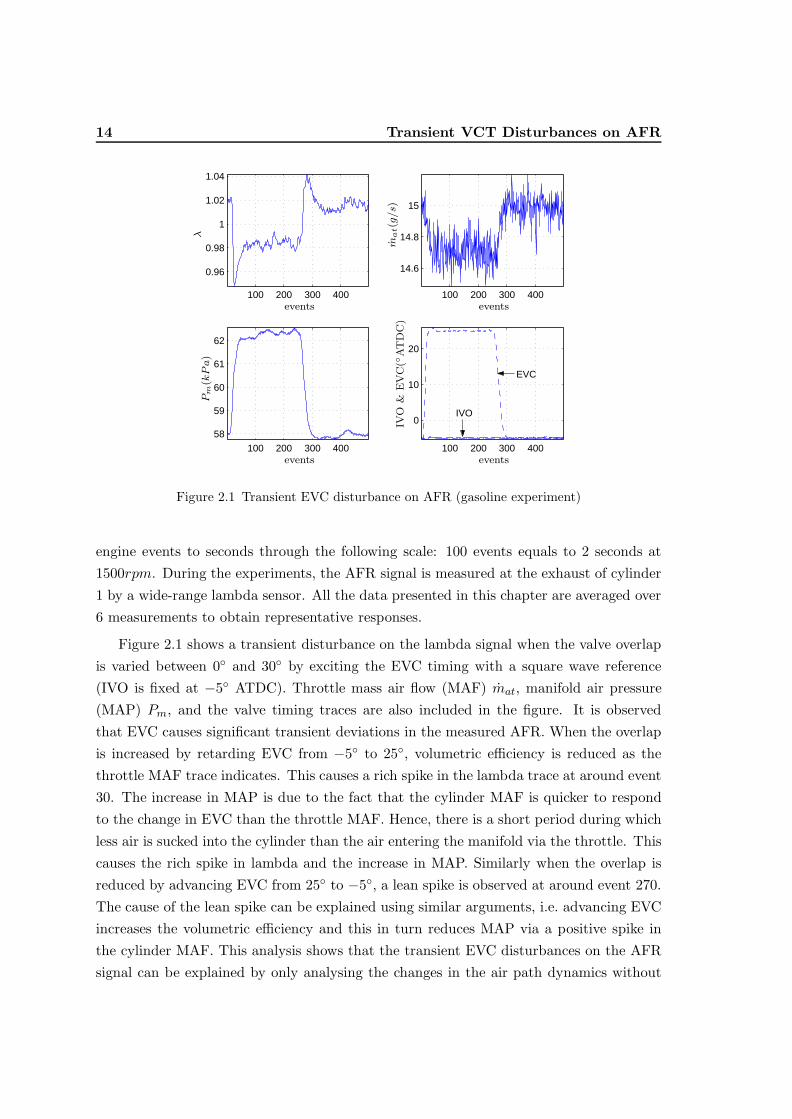
Figure 2.1 Transient EVC disturbance on AFR (gasoline experiment)
engine events to seconds through the following scale: 100 events equals to 2 seconds at1500rpm. During the experiments, the AFR signal is measured at the exhaust of cylinder1 by a wide-range lambda sensor. All the data presented in this chapter are averaged over6 measurements to obtain representative responses.
Figure 2.1 shows a transient disturbance on the lambda signal when the valve overlapis varied between 0◦ and 30◦ by exciting the EVC timing with a square wave reference(IVO is fixed at −5◦ ATDC). Throttle mass air flow (MAF) mat, manifold air pressure(MAP) Pm, and the valve timing traces are also included in the figure. It is observedthat EVC causes significant transient deviations in the measured AFR. When the overlapis increased by retarding EVC from −5◦ to 25◦, volumetric efficiency is reduced as thethrottle MAF trace indicates. This causes a rich spike in the lambda trace at around event30. The increase in MAP is due to the fact that the cylinder MAF is quicker to respondto the change in EVC than the throttle MAF. Hence, there is a short period during whichless air is sucked into the cylinder than the air entering the manifold via the throttle. Thiscauses the rich spike in lambda and the increase in MAP. Similarly when the overlap isreduced by advancing EVC from 25◦ to −5◦, a lean spike is observed at around event 270.The cause of the lean spike can be explained using similar arguments, i.e. advancing EVCincreases the volumetric efficiency and this in turn reduces MAP via a positive spike inthe cylinder MAF. This analysis shows that the transient EVC disturbances on the AFRsignal can be explained by only analysing the changes in the air path dynamics without

2.1. Gasoline Experiments 15
100 200 300 400
0.98
1
1.02
1.04
100 200 300 400
14.6
14.7
14.8
14.9
15
100 200 300 400
−20
−10
0
10
100 200 300 400
59.5
60
60.5
61
IVO
EVC
λ
mat(g/s)
Pm
(kPa)
IVO
&E
VC
(◦A
TD
C)
events events
eventsevents
Figure 2.2 Transient IVO disturbance on AFR (gasoline experiment)
considering any possible effects of the fuel flow dynamics.
A similar experiment is performed by exciting the IVO timing with a square wavereference and keeping the EVC timing fixed at 10◦ ATDC. Figure 2.2 shows that excitingIVO like EVC causes significant transient spikes in the AFR. Extending the overlap intothe exhaust stroke by advancing IVO timing from 10◦ to −20◦ increases the volumetricefficiency, as the slight increase in the throttle MAF trace hints. Thus it is expected thatthere should be a lean spike in the lambda trace at around event 30, if one uses similararguments to the previous EVC experiment case, yet there is a rich spike in the mea-surement instead. Another unexpected behaviour is observed when the overlap is reducedto zero by retarding IVO from −20◦ to 10◦, i.e. a lean spike in lambda at around event270. On the other hand, the MAP trace supports the throttle MAF behaviour, becausewhen the throttle MAF increases, MAP decreases as in the case of EVC disturbance. Yetthe lambda trace has its spikes in opposing directions to that which would be expectedfrom the air flow dynamics. This suggests that there is an extra dynamic effect in themeasurements that is related to neither throttle MAF nor MAP dynamics.
The gasoline experiments above show that not all the transient VCT disturbances onthe AFR signal can be explained by the changes in the air path dynamics. In particularthe transient IVO disturbance on AFR cannot be explained by changes in the air flowdynamics caused by IVO. If the variations in the cylinder MAF cannot explain the observedAFR behaviour, it must be the cylinder fuel flow dynamics that are governing the observed
16 Transient VCT Disturbances on AFR
behaviour. The next section will reveal the transient behaviour of the cylinder MAF underthe VCT excitation through gaseous fuel (propane) experiments in order to understandhow the fuel dynamics behave during the VCT transients.
2.2 Propane Experiments
The same experiments described above are performed with propane as the fuel rather thangasoline. A constant amount of propane is injected into the inlet port of cylinder 1 only.The rate of injection is independent of MAP as the propane injector consisted of a chokedorifice located very close to the injection point. The following assumptions are satisfiedfor the propane experiments,
• There is no wall-wetting dynamics for propane;
• The amount of propane fuel entering the cylinder 1 at each event is almost constantand independent of MAP.
The first assumption can be made since propane is a gaseous fuel. The second assump-tion requires a careful examination. During the propane fuel experiments the rest of thecylinders are run on gasoline through the fuel injectors. If the injected propane staysin the inlet port 1 the assumption would hold and the cylinder propane flow would beindependent of MAP. However, if some of the propane leaks back into the intake mani-fold, the assumption would not hold anymore. This is because the propane leaked intothe manifold would form a premixed air-fuel composition in the intake manifold and theoverall propane flow into the cylinder 1 would depend on MAP. Moreover, this premixedair-fuel composition would also disturb the AFR composition in other cylinders. Since nosuch abnormality in the AFR measurements of the other cylinders are observed duringthe tests, it is concluded that the second assumption holds as well. These two conditionsare required to ensure that the cylinder fuel flow is constant during the experiments. Thismeans that any variations in the observed lambda trace are due to the variations in thecylinder MAF in the following experiments.
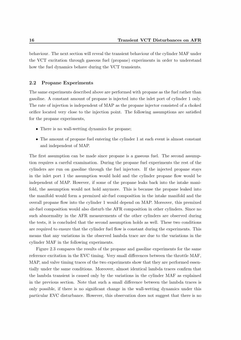
Figure 2.3 compares the results of the propane and gasoline experiments for the samereference excitation in the EVC timing. Very small differences between the throttle MAF,MAP, and valve timing traces of the two experiments show that they are performed essen-tially under the same conditions. Moreover, almost identical lambda traces confirm thatthe lambda transient is caused only by the variations in the cylinder MAF as explainedin the previous section. Note that such a small difference between the lambda traces isonly possible, if there is no significant change in the wall-wetting dynamics under thisparticular EVC disturbance. However, this observation does not suggest that there is no
2.2. Propane Experiments 17
100 200 300 400
0.96
0.98
1
1.02
1.04
100 200 300 400
14.6
14.8
15
100 200 300 400
0
10
20
100 200 300 400
58
59
60
61
62
GasolinePropane
EVC
IVO
λ
mat(g/s)
Pm
(kPa)
IVO
&E
VC
(◦A
TD
C)
events events
eventsevents
Figure 2.3 Transient EVC disturbance on AFR signal (propane experiment)
wall-wetting dynamics for gasoline fuel but only indicates that the wall-wetting dynamicsdo not change under the EVC excitation.
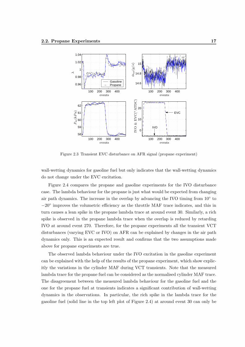
Figure 2.4 compares the propane and gasoline experiments for the IVO disturbancecase. The lambda behaviour for the propane is just what would be expected from changingair path dynamics. The increase in the overlap by advancing the IVO timing from 10◦ to−20◦ improves the volumetric efficiency as the throttle MAF trace indicates, and this inturn causes a lean spike in the propane lambda trace at around event 30. Similarly, a richspike is observed in the propane lambda trace when the overlap is reduced by retardingIVO at around event 270. Therefore, for the propane experiments all the transient VCTdisturbances (varying EVC or IVO) on AFR can be explained by changes in the air pathdynamics only. This is an expected result and confirms that the two assumptions madeabove for propane experiments are true.
The observed lambda behaviour under the IVO excitation in the gasoline experimentcan be explained with the help of the results of the propane experiment, which show explic-itly the variations in the cylinder MAF during VCT transients. Note that the measuredlambda trace for the propane fuel can be considered as the normalised cylinder MAF trace.The disagreement between the measured lambda behaviour for the gasoline fuel and theone for the propane fuel at transients indicates a significant contribution of wall-wettingdynamics in the observations. In particular, the rich spike in the lambda trace for thegasoline fuel (solid line in the top left plot of Figure 2.4) at around event 30 can only be

18 Transient VCT Disturbances on AFR
100 200 300 400
0.96
0.98
1
1.02
1.04
1.06
100 200 300 400
14.6
14.7
14.8
14.9
15
15.1
100 200 300 400
−20
−10
0
10
100 200 300 400
58
59
60
61
62
GasolinePropane
EVC
IVO
λ
mat(g/s)
Pm
(kPa)
IVO
&E
VC
(◦A
TD
C)
events events
eventsevents
Figure 2.4 Transient IVO disturbance on AFR signal (propane experiments)
explained with a big increase in the cylinder fuel flow when the normalised cylinder MAFis going through a positive transient as indicated by the measured lambda trace for thepropane fuel (dashed-dotted line in the top left plot of Figure 2.4). Since the injectedfuel is constant during the experiments, the extra fuel can only come from the fuel puddleitself. This implies a decrease in the fuel puddle size at around event 30. Similarly, a leanspike in the lambda trace for the gasoline fuel at around event 270 while the normalisedcylinder MAF is going through a negative transient shows a significant reduction in thecylinder fuel flow. This indicates an increase in the fuel puddle size at around event 270.
So far only the transient behaviour of the results shown in Figure 2.4 has been discussedsince it is the main focus of this work. However there is some steady state inconsistencyin the measurements. In particular throttle MAF readings are in disagreement with thegasoline lambda readings, i.e.when throttle MAF increases the gasoline lambda goes richat steady state and vice versa. Note that this is a very unexpected behaviour sincethe fuel injection timings were constant during the experiments. The data presented inFigures 2.3- 2.4 suggest that the propane lambda readings are reliable as they agree withall the other sensor measurements. This raises the question whether the injected fuel wasreally constant during the experiment shown in Figure2.4. One possibility is that therewas a hysteresis in the fuel pressure control valve which is referenced to manifold pressure.Thus pressure spikes in Figure 2.4 in MAP could cause slight changes in injected fuelamount. This discussion is not exhaustive and further work is definitely required in order

2.2. Propane Experiments 19
0 100 200 300 400 50040
45
50
55
60EVC excited, IVO=−5
0 100 200 300 400 50040
45
50
55
60IVO excited, EVC=10
100 200 300 400 500
0
10
20
100 200 300 400 500
−20
−10
0
10
Inle
tP
ort
Tem
per
atu
re(◦C
)
Inle
tP
ort
Tem
per
atu
re(◦C
)
eventsevents
EV
C(◦
AT
DC
)
IVO
(◦A
TD
C)
Figure 2.5 Variations in the inlet port temperature at 40kPa under VCT excitation
to determine the causes of this steady state mismatch in the measurements. However thisproblem will not be further pursued in this work due to strict time limitations.
It is evident from the above experiments that varying the valve overlap via the IVOtiming has a significant effect on the fuel puddle size, whereas varying it via the EVCtiming has a negligible one. This difference cannot be explained by variations in eitherthe throttle MAF or MAP dynamics. A possible explanation is given below. During theexperiments the gas temperature around the inlet port of the cylinder 1 is also measured bya thermocouple (K-type/insulated/0.5mm) as depicted in Figure 2.5. The measurementsshow that both the EVC and IVO timing change the inlet port temperature. In particularincreasing the valve overlap increases the inlet port temperature, since there is more backflow of residual gases into the inlet port and intake manifold. However, data also showthat early IVO causes a much bigger change in the port temperature than the late EVCfor the same overlap change, especially at low loads. With early IVO, the piston is movingupwards for the most of the overlap period and is pushing the residual gases into theintake manifold. On the other hand, with late EVC, the piston is moving downwardsfor most of the overlap, and therefore pulling the residual gases into the cylinder. Sucha difference in the amount of residual gas pushed back into the inlet port can explainthe smaller increase in the temperature by retarding EVC. Furthermore, the fact thatthe EVC excitation causes smaller variations in the port temperature can explain whyexciting EVC does not change the fuel puddle size as much. Note that it is expected that
20 Transient VCT Disturbances on AFR
the actual mean temperature variation of the gas around the intake valves would be largersince the measurements were taken 4-5cm upstream from the injectors. Also there mustbe a cyclic temperature variation which is not resolved with the thermocouple here due tothe time constant of the thermocouple (appeared to be around 0.3-0.4s). Higher frequencyresponse temperature measurements by a faster sensor might reveal other effects.
2.3 Comments
The propane experiments give a clear indication of the normalised cylinder MAF behaviourduring the VCT transients. This will give us confidence later on, when the validation of thecylinder MAF model will be performed against the traces from the propane experiments.The gasoline and propane experiments together not only show that the VCT mechanismcauses significant transient deviations in AFR but also indicate that the fuel puddle sizevaries significantly during the IVO timing transients. The empirical evidence showing thatthe fuel puddle size changes with the valve timings especially with the IVO timing is thefirst published result indicating significant changes in the wall-wetting dynamics underVCT transients to the author’s knowledge. Furthermore, the experiments indicate thateven a perfect cylinder MAF predictor alone cannot achieve a tight transient AFR controlin a TI-VCT engine due to significant variations in the cylinder fuel flow rate during thetransients. Such a change in fuel flow cannot be compensated for without an accuratewall-wetting model, which must predict the variations in the fuel puddle parameters withthe valve timings. Hence further investigation of the AFR path in TI-VCT engines isimperative, if a satisfactory transient AFR control is to be accomplished. The results ofthis chapter have recently been published in [GFGC02].

3
Modelling and Identification of the AFR Path
Empirical results of the previous chapter have shown that both air-and fuel dynamics playan important role in shaping the transient AFR behaviour under the VCT disturbances.These dynamics and their relationships with the valve timings must be captured by anAFR path model if good AFR regulation is desired. This chapter presents a mean valueAFR path model and proposes schemes for identification of its parameters, for which bothlocal (linear) and global identification methods are employed.
A mean value engine model describes the engine dynamics with limited bandwidth,equivalent to considering the mean behaviour of the state variables over engine events.So-called standard mean value engine models exist in the literature for PFI engines [HS90,MH92, CM00]. They usually include the models of the air flows, intake manifold, wall-wetting of the fuel, torque generation and engine speed. Early publications also includemodels for the carburetor and fuel flow in the intake manifold [Dob80,Pow87,PC87].
There are two types of relationships in a mean value engine model. The first type isthe very fast dynamics that achieve equilibrium in a few engine events. Such dynamicsare usually ignored and static mappings (look-up tables or polynomial regression fittings)are used to describe them. For example, the relationship from throttle position (TP)and MAP to throttle MAF is considered as instantaneous in the mean value model. Thesecond type of relationships are relatively slow processes with time constants around tensor hundreds of engine events. They are described by differential equations and constitutethe state variables of the engine model. In general most of the flows (apart from fuelflow), torque and emission generations are modelled as instantaneous relationships. Onthe other hand, the manifold pressure, fuel puddle (film) mass and engine speed (denotedas N) are the most common state (dynamic) variables in the mean value engine model.
Engine models can be constructed either in the time domain or crank angle domain. Itis possible to transform a differential equation in one domain to another with the knowledge
21

22 Modelling and Identification of the AFR Path
AFR
MAP
SensorAFR
3
4
2
1Temperature
Sensor
SensorMAF
Sensor
SensorsVCT
SensorTP
Sensor
ConverterCatalytic
Figure 3.1 Main sensors used in the AFR path identification
of engine speed
dθ
dt= 6N, (3.1)
where θ is in crank angle degrees, t is in seconds and N is in rpm. Since many engineprocesses are periodic in the crank angle domain, identification of the models in thisdomain has advantages over identification of models in the time domain. For example,most of the dynamics vary less in the crank angle domain than in the time domain [CC86];this is very desirable when identifying a parameter-varying model. Therefore, the AFRpath model for the TI-VCT engine will be constructed in the crank angle domain witha sampling angle of 180 crank angle degrees, i.e. an engine event. Such models are alsoknown as event based discrete-time mean value engine models.
Figure 3.1 shows a sketch of the positions of the main sensors used in the identificationof the AFR path. More detailed information about the engine and facilities can be foundin Appendix A. The next section will present the identification and partial validationof the air path dynamics, which are composed of the throttle MAF, cylinder MAF andMAP dynamics. Section 3.2 will expose the identification and partial validation of thefuel path dynamics, which are composed of the injection delay, wall-wetting dynamics,transport delay, gas mixing, and the lambda sensor dynamics. Local linear identificationmethods are used for identifying the parameters of the fuel path except for the wall-wettingparameters, which are identified by a global identification scheme. Finally, the completeAFR path model will be validated under transient VCT operation in Section 3.3. Notethat all the identification and validation experiments are performed at 1500rpm.
3.1. Air Path Dynamics 23
3.1 Air Path Dynamics
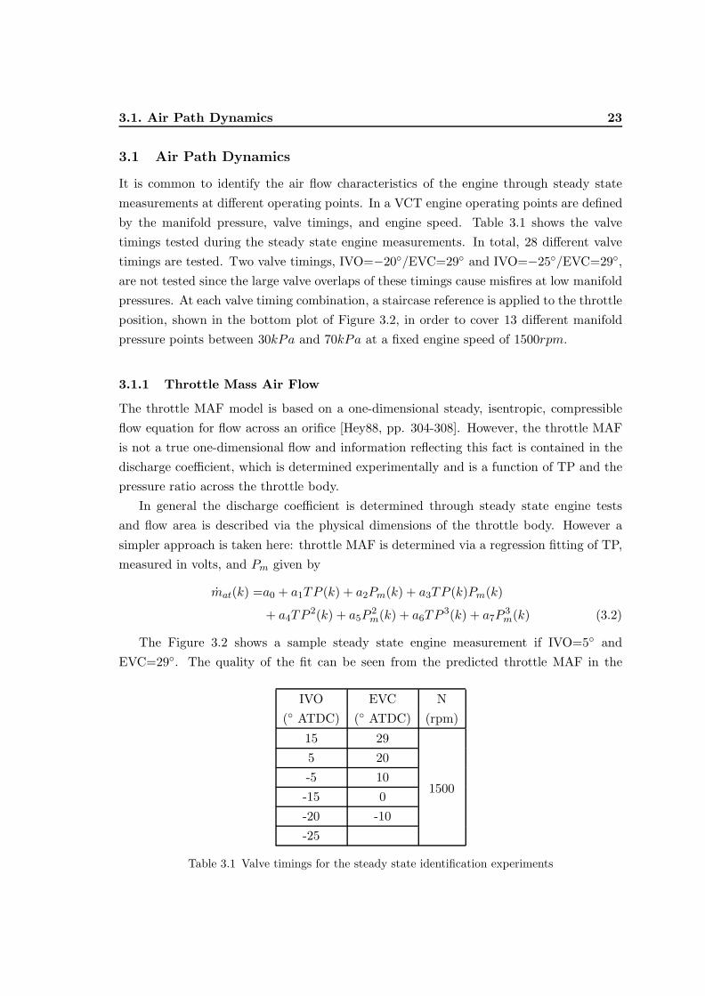
It is common to identify the air flow characteristics of the engine through steady statemeasurements at different operating points. In a VCT engine operating points are definedby the manifold pressure, valve timings, and engine speed. Table 3.1 shows the valvetimings tested during the steady state engine measurements. In total, 28 different valvetimings are tested. Two valve timings, IVO=−20◦/EVC=29◦ and IVO=−25◦/EVC=29◦,are not tested since the large valve overlaps of these timings cause misfires at low manifoldpressures. At each valve timing combination, a staircase reference is applied to the throttleposition, shown in the bottom plot of Figure 3.2, in order to cover 13 different manifoldpressure points between 30kPa and 70kPa at a fixed engine speed of 1500rpm.
3.1.1 Throttle Mass Air Flow
The throttle MAF model is based on a one-dimensional steady, isentropic, compressibleflow equation for flow across an orifice [Hey88, pp. 304-308]. However, the throttle MAFis not a true one-dimensional flow and information reflecting this fact is contained in thedischarge coefficient, which is determined experimentally and is a function of TP and thepressure ratio across the throttle body.
In general the discharge coefficient is determined through steady state engine testsand flow area is described via the physical dimensions of the throttle body. However asimpler approach is taken here: throttle MAF is determined via a regression fitting of TP,measured in volts, and Pm given by
mat(k) =a0 + a1TP (k) + a2Pm(k) + a3TP (k)Pm(k)
+ a4TP2(k) + a5P
2m(k) + a6TP
3(k) + a7P3m(k) (3.2)
The Figure 3.2 shows a sample steady state engine measurement if IVO=5◦ andEVC=29◦. The quality of the fit can be seen from the predicted throttle MAF in the
IVO EVC N(◦ ATDC) (◦ ATDC) (rpm)
15 295 20-5 10-15 0
1500
-20 -10-25
Table 3.1 Valve timings for the steady state identification experiments

24 Modelling and Identification of the AFR Path
1000 2000 3000 4000 5000 6000 70008
1012141618
1000 2000 3000 4000 5000 6000 7000
40
50
60
70
1000 2000 3000 4000 5000 6000 70001.1
1.2
1.3
1.4
events
Measured Predicted
mat(g/s)
Pm
(kPa)
TP
(V)
Figure 3.2 A sample steady state engine test for IVO=5◦and EVC=29◦
top plot. Although, the figure shows that the model has a good steady state fit, the tran-sient accuracy of the model needs to be checked against the independent validation datato make sure that the transient throttle MAF behaviour is captured correctly.
The overall measurements and the fitted surface are plotted in Figure 3.3, where thequality of the fit can be seen. In fact, the worst case error between the model and data isno larger than 2.6 %.
Transient Validation
It is an established assumption for mean value models that the throttle MAF is governedby the throttle position and manifold pressure. In a VCT engine variations in valve timingschange the manifold pressure and therefore the throttle MAF. It is important that theproposed model can predict the transient behaviour observed in the measured throttleMAF induced by the VCT mechanism through the manifold pressure correctly. In orderto confirm this, the throttle flow model is validated against independent transient data,which are averaged over 4 measurements to improve the signal-to-noise ratio. The firstvalidation data are shown in Figure 3.4, in which the EVC timing follows a square referencesignal while the IVO timing is fixed at −5◦ ATDC. Although there is some offset in theprediction, the transient behaviour of the actual data is captured in the model.
The final transient validation is performed for the IVO excitation, while EVC is fixedat 10◦ ATDC. The model again correctly predicts actual behaviour shown in Figure 3.5,which reveals that, at low loads, IVO excitation does not affect the throttle MAF.

3.1. Air Path Dynamics 25
1.151.2
1.251.3
1.351.4
40
50
60
70
5
10
15
20
Worst case error is 2.6%
ActualFit
mat(g/s)
Pm (kPa) TP (V )
Figure 3.3 Steady state measurements of the throttle MAF and the model fit
0 50 100 150 200 250 300 350 400 450 5008.5
9
9.5
50 100 150 200 250 300 350 400 45039
40
41
42
43
50 100 150 200 250 300 350 400 450
0
10
20
events
Measured Predicted
mat(g/s)
Pm
(kPa)
EVC
(◦ATDC
)
Figure 3.4 Transient validation of the throttle MAF (EVC excitation)

26 Modelling and Identification of the AFR Path
0 50 100 150 200 250 300 350 400 450 5009.6
9.8
10
10.2
50 100 150 200 250 300 350 400 450
41
42
43
50 100 150 200 250 300 350 400 450−20
−10
0
10
events
Measured Predicted
mat(g/s)
Pm
(kPa)
IVO
(◦ATDC
)
Figure 3.5 Transient validation of the throttle MAF model (IVO excitation)
3.1.2 Cylinder Mass Air Flow
For a conventional PFI engine the cylinder MAF is considered to be the main disturbancefor the AFR loop, hence its precise modelling is essential. Conventional steady state enginemeasurements are capable of describing the engine breathing performance with remarkableaccuracy even during fast transient operation, despite the complex nature of the pulsatingair flow out of the manifold. It is common to model cylinder MAF by the so-calledspeed-density formulation [MH92, CVH00], in which the volumetric efficiency is mappedas a function of the manifold pressure, ambient pressure and ambient temperature. For adual-equal VCT engine, the cylinder MAF is modelled as a polynomial in cam phasing,manifold pressure and engine speed in [SCGF98]. Here, a slightly different polynomialapproach is proposed. The data used for cylinder MAF identification are the same asthe steady state data used for the throttle MAF identification above (see Table 3.1 andFigure 3.2). Figure 3.6 shows that the manifold pressure is the main factor determiningthe amount of air sucked into cylinders when the engine speed is constant. On the otherhand, the valve timings seem to mainly vary the offset of this almost linear relationship.Each plot shows how the cylinder MAF characteristics varies with MAP and IVO timingat a fixed EVC timing. The solid lines, which change significantly with the valve timings,are the fitted quadratic polynomials for each valve timing. Thus, the cylinder MAF ismodelled as a quadratic in MAP, where the coefficients are functions of the valve timings
mac(k) = l0a(k) + l1a(k)Pm(k) + l2a(k)P 2m(k) (3.3)
3.1. Air Path Dynamics 27
40 50 60 70
10
12
14
16
18
EVC =−10 ° ATDC
40 50 60 70
10
12
14
16
18
EVC =0 ° ATDC
40 50 60 70
10
12
14
16
18
EVC =10 ° ATDC
40 50 60 70
10
12
14
16
18EVC =20 ° ATDC
40 50 60 70
10
12
14
16
EVC =29 ° ATDC
−1 −0.5 0 0.5 1−1
−0.5
0
0.5
1
IVO −25IVO −20IVO −15IVO −5 IVO 5 IVO 15
mac(g/s
)
mac(g/s
)
mac(g/s
)
mac(g/s
)
mac(g/s
)
Pm (kPa)
Pm (kPa)Pm (kPa)
Pm (kPa)Pm (kPa)
Legend
Leg
end
Figure 3.6 Identification data and the model fit for mac

28 Modelling and Identification of the AFR Path
andlia(k) = fi(IV O(k), EV C(k)), i = 0, 1, 2.
Note that a quadratic model is used to ensure that even the weak second order effectsare captured by the model. Each coefficient lia is a complicated nonlinear function of thevalve timings IVO and EVC. They are depicted in Figure 3.7. The plots on the left columnshow the identified raw surfaces of coefficients with respect to valve timings, whereas theones on the right show the same surfaces but smoothed. The identified coefficient surfaceshave multiple maxima, which make them difficult to model precisely without using highorder polynomials. The dominant term is l1 as expected and its value is fairly smoothacross the valve timing envelope. On the other hand, the values of the l0 and l2 termsseem to vary significantly with valve timings. In order to maximise the accuracy of themodel, the coefficients lia are stored in look-up tables.
Finally, the identified cylinder MAF surfaces are plotted in Figure 3.8, where eachsurface is given for a fixed EVC timing. The main trends in cylinder MAF model are:
i. MAP is the main factor in determining the cylinder MAF;
ii. Retarding EVC from −10◦ to 29◦ reduces the flow;
iii. IVO has a more complicated effect, almost quadratic, on the cylinder MAF andmoving IVO to both ends reduces the flow;
The identification is deemed to be successful with a worst case error of 2.3 % between themodel and data.
Transient Validation
The accurate modelling of the cylinder MAF is very crucial in building a reliable AFRpath model of the TI-VCT engine. The transient validation of the cylinder MAF modelis achieved by comparing the model predictions with the lambda traces of the propaneexperiments discussed in the previous chapter. Recall that the lambda traces from thepropane experiments represent the transient behaviour of the normalised cylinder MAF.The first validation data are given in Figure 3.9 for varying EVC and IVO=-5◦. For agood model the empirical lambda trace should be a delayed and low-pass filtered formof the predicted normalised cylinder MAF. This is due to the transport delay and extradynamics at the exhaust such as the lambda sensor dynamics which cause the low-passfiltering. Figure 3.9 shows that the prediction of the model is precise both during retardingand advancing of the EVC timing.
The second transient validation, where data is again taken from the previous propaneexperiments, is done against the IVO timing excitation with EVC=10◦. The transient
3.1. Air Path Dynamics 29
−20−10
010
−100
1020
−4
−3
−2
−1
x 10−3
Raw Data
−20−10
010
−100
1020
−5
−4
−3
−2
−1
x 10−3
Smoothed Data
−20−10
010
−100
1020
2.83
3.23.43.63.8
x 10−4
−20−10
010
−100
1020
2.5
3
3.5
4
x 10−4
−20−10
010
−100
1020
−10
−8
−6
−4
−2
x 10−7
−20−10
010
−100
1020
−10
−5
0
x 10−7
l 0l 0
l 1l 1
l 2l 2
IV O(◦ATDC)IV O(◦ATDC)
IV O(◦ATDC)IV O(◦ATDC)
IV O(◦ATDC)IV O(◦ATDC)
EVC(◦ATDC)EVC(◦ATDC)
EVC(◦ATDC)EVC(◦ATDC)
EVC(◦ATDC)EVC(◦ATDC)
Figure 3.7 Coefficients of the quadratic cylinder MAF model

30 Modelling and Identification of the AFR Path
3040
5060
70
−30−20
−100
1020
4
6
8
10
12
14
16
18
2920100
−10
Worst case error is 2.3%mac
(g/s)
Pm (kPa)IV O(◦ATDC)
EVC (◦ATDC)
Figure 3.8 Identified cylinder MAF surfaces
50 100 150 200 250 300 350 400 450
0.95
1
1.05
50 100 150 200 250 300 350 400 450
39
40
41
42
43
50 100 150 200 250 300 350 400 450
0
10
20
events
λandmac
Measured λPredicted mac
Pm
(kPa)
EVC
(◦ATDC
)
Figure 3.9 Transient validation of the cylinder MAF model (EVC excitation)
3.1. Air Path Dynamics 31
50 100 150 200 250 300 350 400 450
0.96
0.98
1
1.02
1.04
50 100 150 200 250 300 350 400 450
59
60
61
50 100 150 200 250 300 350 400 450−20
−10
0
10
events
λandmac Measured λ
Predicted mac
Pm
(kPa)
IVO
(◦ATDC
)
Figure 3.10 Transient validation of the cylinder MAF model (IVO excitation)
agreement between the measured lambda and the predicted normalised cylinder MAF isaccurate in the sense that measured lambda looks like a filtered form of the predicted airflow as can be seen in Figure 3.10. The model predicts precisely not only the positivespike in the normalised cylinder MAF when IVO is advanced but also the negative spikewhen IVO is retarded. These transient validation results increase the confidence in theproposed cylinder MAF model defined in (3.3).
3.1.3 Intake Manifold Model
The true nature of the air dynamics in the intake manifold is very complex. The intakemanifold consists of a plenum with individual runners feeding branches which lead toindividual cylinders. It is common in AFR control applications to use a lumped parametermodel and assuming uniform pressure and temperature. The most common mean valuemodel of the intake manifold is the isothermal filling-emptying model [Hey88, MH92],where manifold pressure is the only state variable. Such a model can be derived byapplying conservation of mass and the ideal gas law. Isothermal models assume that theintake manifold temperature is known and constant.
More recent studies in [CM00, Hen01] also propose adiabatic manifold models, whereboth the conservation of mass and energy are applied in order to derive the governingequations. The main difference between the isothermal and adiabatic models is an ex-tra differential equation describing the dynamics of intake manifold temperature in the
32 Modelling and Identification of the AFR Path
adiabatic models. Adiabatic models assume both the manifold pressure and manifoldtemperature as time-varying, but assume negligible heat transfer between the manifoldand its environment. On the other hand, isothermal models assume a constant manifoldtemperature throughout the inlet manifold. In [CM00] it is shown that better predictionsof the air flow dynamics can be achieved, if the adiabatic manifold models are employed.
Here the first approach is taken and the event based discrete-time filling-emptyingintake manifold model is used to describe the manifold dynamics as
Pm(k + 1) = Pm(k) +TsRTm6NVm
(mat(k)− mac(k)) , (3.4)
where Ts is sampling time in events, Vm is the manifold volume, and Tm is the manifoldtemperature in Kelvin. Since both the throttle MAF and cylinder MAF have alreadybeen modelled, the intake manifold model can be used without any further engine testsby substituting the appropriate values of the parameters in (3.4). However, the accuracyof the model should be validated.
Transient Validation
The manifold engine model is validated against three different transient excitations. Notethat all the presented validation data are averaged over 4 measurements. The first set ofvalidation data shown in Figure 3.11 is taken from an engine test where the EVC timingis excited by a square wave reference signal as before. Although there is some offset in thepredictions, the model captures both the MAP and throttle MAF transients accurately.The transient validation data for IVO excitation are depicted in Figure 3.12. Again somesteady state errors are present in the predictions but the transient characteristics of thedata are captured well by the model. In the final validation test it is investigated whetherthe model can predict the variations in MAP under TP excitation with constant valvetimings. Once again the model predictions of the MAP and throttle MAF agree with theobserved transient behaviour well in Figure 3.13.
The validation of the manifold model completes the mean value modelling of the airpath dynamics for the AFR control problem. The partial validation of the transientaccuracy of each model for different excitations gives promising results and increases theconfidence in the use of the model for designing a feedforward controller. Note thatneither of the MAF models take into account the ambient air temperature. Hence steadystate errors are expected in the models’ predictions when the ambient air temperature isdifferent from its value during the identification tests.
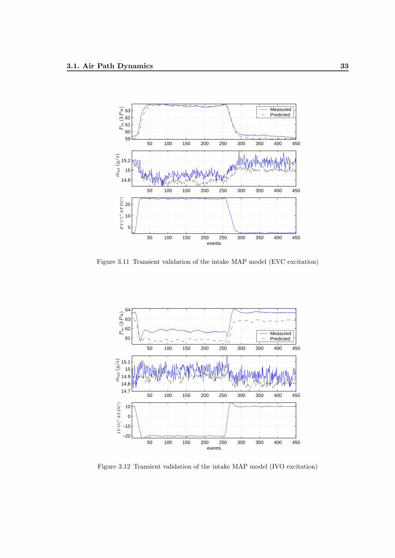
3.1. Air Path Dynamics 33
50 100 150 200 250 300 350 400 45059
60
61
62
63 Measured Predicted
50 100 150 200 250 300 350 400 450
14.8
15
15.2
50 100 150 200 250 300 350 400 450
0
10
20
events
mat
(g/s)
Pm
(kPa)
EVC
(◦ATDC
)
Figure 3.11 Transient validation of the intake MAP model (EVC excitation)
50 100 150 200 250 300 350 400 450
61
62
63
64
Measured Predicted
50 100 150 200 250 300 350 400 45014.7
14.8
14.9
15
15.1
50 100 150 200 250 300 350 400 450−20
−10
0
10
events
mat
(g/s)
Pm
(kPa)
IVO
(◦ATDC
)
Figure 3.12 Transient validation of the intake MAP model (IVO excitation)

34 Modelling and Identification of the AFR Path
50 100 150 200 250 300 350 400 450
54
56
58Measured Predicted
50 100 150 200 250 300 350 400 450
13
13.5
14
14.5
50 100 150 200 250 300 350 400 450
1.31
1.32
1.33
1.34
events
mat
(g/s)
Pm
(kPa)
TP
(V)
Figure 3.13 Transient validation of the intake MAP model (TP excitation)
3.2 Fuel Path Dynamics
The fuel path, depicted in Figure 3.14, is composed of the injection delay, wall-wettingdynamics, transport delay, gas mixing dynamics and lambda sensor dynamics. The injec-tion fuel pulse-width is denoted as FPW in the following. Note that the model output ischosen as φ rather than λ in order to have the controller input FPW entering the modellinearly. The injection delay is the time between the sampling of the lambda sensor byengine control unit (ECU) and the time at which the in-cylinder AFR builds up to its finalvalue. This delay is important, because any disturbance that may alter the AFR duringthis period cannot be compensated for by the controller. The injection delay depends onthree parameters [CVH00]:
• Computation duration: This is the time it takes for the ECU to compute one stepof the control strategy.
• Injection duration: The flow out of the injector is constant and it is the durationof the injection pulse that determines the quantity of fuel injected. This pulse isusually between 12 and 450 crank-angle degrees.
• Start of injection delay: In order to achieve low emissions, the quality of air-fuelmixture is also important, i.e. as much fuel as possible should enter into the cylindersin vapour form. As the heat from the intake air is negligible compared to the heatabsorbed from the walls, injecting most of the fuel on closed intake valves is a

3.2. Fuel Path Dynamics 35
Injection
Delay
Wall
DynamicsSensor
Dynamics DelayTransport Gas Mixing Wetting
Dynamics mfc
mac
φc φx
×÷
FPW
Figure 3.14 Fuel path dynamics for one cylinder
requirement.
The transport delay, which has constant and variable parts, is the main delay in theloop. The constant part is around two engine events long and is due to the compressionand expansion strokes. The variable part is the time it takes for the burned gases in thecylinders to have an impact on the lambda sensor once the exhaust valves are open. Thisdelay is inversely proportional to the MAF. Overall the transport delay varies from threeevents to several events depending on the engine speed and manifold pressure (also calledengine load).
The wall-wetting dynamics describe the fact that not all the injected fuel enters intothe cylinder immediately. Some of the fuel impinges onto the inlet port wall and en-ters the cylinder gradually through evaporation and dribble. The model proposed byAquino [Aqu81] is widely quoted in the literature [HO81, TG93, PD93], and can be de-scribed in discrete-time as:
mff (k + 1) = (1− τ)mff (k) + Xmfi(k) (3.5)
mfc(k) = τmff (k) + (1−X )mfi(k) (3.6)
The input to the model is the injected fuel mass mfi and the output is the fuel massentering into the cylinder mfc. A fraction X of the injected fuel is deposited on the wallsto increase the fuel puddle mass in the intake port together with a portion 1−τ of the fuelpuddle itself. At the same time, a fraction τ of the fuel puddle mass evaporates and entersinto the cylinder together with the remainder portion 1−X of the injected fuel. Note thatthis model satisfies conservation of mass and therefore makes no contribution at steadystate. A second order wall-wetting model with three parameters has been introducedby Turin et al. [TCG94]. Wall-wetting models with two fuel puddles have been publishedin [OG94,ORG97]. In a multi-cylinder PFI engine there are as many wall-wetting dynamicsas the number of the cylinders in the engine. Thus, a model with multiple parallel systemsshould be considered. A simplified multiplexing fuel path model for a 4-cylinder engineis shown in Figure 3.15. This model can predict the resonance modes in the frequencyresponse of the AFR path caused by the multiplexing nature of a multi-cylinder engine.
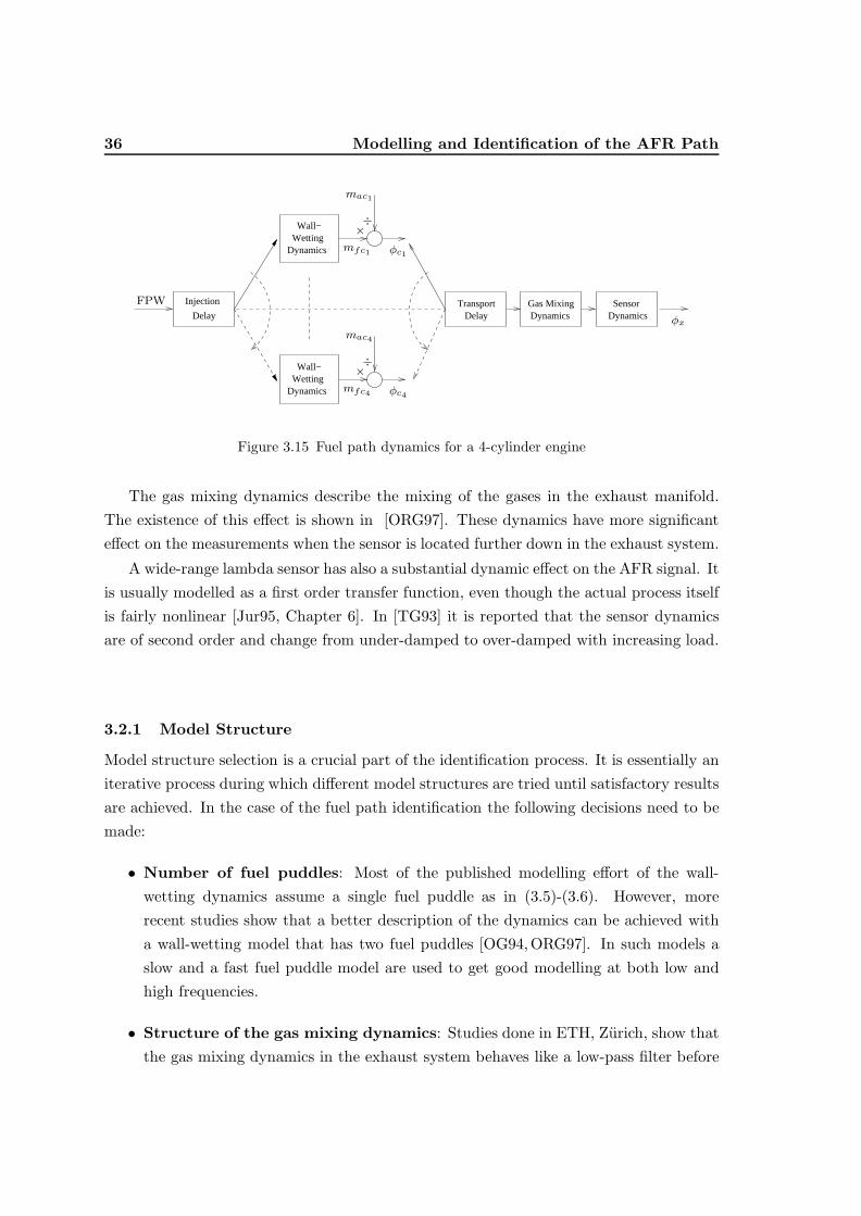
36 Modelling and Identification of the AFR Path
Injection
Delay DynamicsSensor
Dynamics DelayTransport Gas Mixing
WettingDynamics
WettingDynamics
Wall−
Wall−
mfc1
mac1
φc1
mfc4
mac4
φc4
φx
×
×
÷
÷
FPW
Figure 3.15 Fuel path dynamics for a 4-cylinder engine
The gas mixing dynamics describe the mixing of the gases in the exhaust manifold.The existence of this effect is shown in [ORG97]. These dynamics have more significanteffect on the measurements when the sensor is located further down in the exhaust system.
A wide-range lambda sensor has also a substantial dynamic effect on the AFR signal. Itis usually modelled as a first order transfer function, even though the actual process itselfis fairly nonlinear [Jur95, Chapter 6]. In [TG93] it is reported that the sensor dynamicsare of second order and change from under-damped to over-damped with increasing load.
3.2.1 Model Structure
Model structure selection is a crucial part of the identification process. It is essentially aniterative process during which different model structures are tried until satisfactory resultsare achieved. In the case of the fuel path identification the following decisions need to bemade:
• Number of fuel puddles: Most of the published modelling effort of the wall-wetting dynamics assume a single fuel puddle as in (3.5)-(3.6). However, morerecent studies show that a better description of the dynamics can be achieved witha wall-wetting model that has two fuel puddles [OG94, ORG97]. In such models aslow and a fast fuel puddle model are used to get good modelling at both low andhigh frequencies.
• Structure of the gas mixing dynamics: Studies done in ETH, Zurich, show thatthe gas mixing dynamics in the exhaust system behaves like a low-pass filter before

3.2. Fuel Path Dynamics 37
Test OVL IVO EVC Pm Nnumber (degrees) (◦ ATDC) (◦ ATDC) (kPa) (rpm)
1 15 -5 10 302 0 -5 -53 15 -5 104 30e -5 25 405 30i -20 106 35 -25 10 15007 0 -5 -58 15 -5 109 30e -5 25 6010 30i -20 1011 35 -25 10
Table 3.2 Operating points of the fuel path identification experiments
the lambda sensor [ORG97,ORSG98]. However, whether or not these dynamics varywith the operating point should be investigated together with the order of the filter.
• Structure of the lambda sensor dynamics: The order of the sensor transferfunction and whether or not the dynamics vary with the operating point should beinvestigated.
Answers to these questions are sought through performing different types of identificationexperiments and analysing the empirical data. The operating points, at which the exper-iments are performed, are given in Table 3.2. The valve overlap is denoted as OVL in thetable. At each operating point only the amount of fuel injection is varied in order to excitethe fuel path. The valve timings are varied from no overlap to increased overlap valueswith different valve timing combinations. For example 30◦ of overlap can be achieved byeither retarding EVC or advancing IVO. Both cases are included in the experiments andare labelled as 30e for retarded EVC and 30i for advanced IVO. Furthermore, the experi-ments are repeated at different manifold pressures to investigate the effect of the load inthe fuel path as well as the effect of the VCT. Only one overlap timing is tested at 30kPa,because it is not possible to increase the overlap further at very low loads without causingengine misfires.
Step responses of the fuel path dynamics are measured by exciting the fuel injectorswith a square wave FPW. The peak to peak magnitude of the FPW is kept around 8 % ofits nominal value to achieve local linearity in the input-output data. The AFR deviationsare measured by a wide-range lambda sensor at the exhaust of cylinder 1. Moreover,

38 Modelling and Identification of the AFR Path
10 20 30 40 50 60 700
0.1
0.2
0.3
0.4
0.5
0.6
0.7
0.8
0.9
1
cycles (4 events)
ovl=15 30kPa ovl=0 40kPa ovl=15 40kPa ovl=30
e 40kPa
ovl=30i 40kPa
ovl=35 40kPa ovl=0 60kPa ovl=15 60kPa ovl=30
e 60kPa
ovl=30i 60kPa
ovl=35 60kPa
Norm
ali
sedφ
Figure 3.16 Normalised step responses of the fuel path
the data are averaged over many measurements to get a representative response. Thenormalised φ step responses are plotted in Figure 3.16, where each step response is anaverage of 26 steps. All the responses have second order over-damped characteristics witha delay as expected. The data show variations in step responses with operating point. Itis observed that the speed of the response is dependent on both the manifold pressure andvalve timings. For example, as the load increases the responses get faster.
Although step responses are useful to observe the low frequency characteristics ofthe system such as time delay, dominant time constant, rise and settling times, they donot contain much information about the higher frequency dynamics. An ideal excitationfor a wide-range frequency identification is a sum of sinusoids [Lju99, p. 423]. Hence,further experiments are performed by exciting the fuel injectors with a sum of sinusoidsFPW. Details of how to construct such an excitation signal are given in Appendix B.The measurements are taken by a wide-range lambda sensor after the confluence pointof the exhaust runners, i.e. these measurements represent the mean behaviour of thefour cylinders rather than just one. The measured frequency response of the fuel path atdifferent operating points are given in Figure 3.17. The frequency responses are calculatedvia a Fourier analysis of the input-output data. It is seen that the magnitudes and phasesof the responses have substantial variations at high frequencies (> 0.1rad/event). As theMAP increases the response gets faster as evident from the decreasing phase, which isa direct result of the shorter transport delays at high manifold pressures. Moreover, the
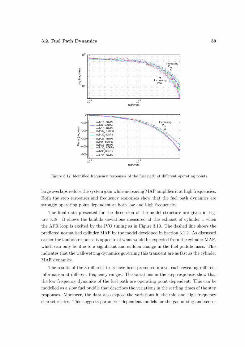
3.2. Fuel Path Dynamics 39
10−2
10−1
10−1
100
rad/event
Log
Mag
nitu
te
10−2
10−1
−500
−400
−300
−200
−100
0
rad/event
Pha
se (
degr
ees)
ovl=15 30kPa ovl=0 40kPa ovl=15 40kPa ovl=30
e 40kPa
ovl=30i 40kPa
ovl=35 40kPa ovl=0 60kPa ovl=15 60kPa ovl=30
e 60kPa
ovl=30i 60kPa
ovl=35 60kPa
Increasing P
m
Increasing P
m
Increasing OVL
Figure 3.17 Identified frequency responses of the fuel path at different operating points
large overlaps reduce the system gain while increasing MAP amplifies it at high frequencies.Both the step responses and frequency responses show that the fuel path dynamics arestrongly operating point dependent at both low and high frequencies.
The final data presented for the discussion of the model structure are given in Fig-ure 3.18. It shows the lambda deviations measured at the exhaust of cylinder 1 whenthe AFR loop is excited by the IVO timing as in Figure 3.10. The dashed line shows thepredicted normalised cylinder MAF by the model developed in Section 3.1.2. As discussedearlier the lambda response is opposite of what would be expected from the cylinder MAF,which can only be due to a significant and sudden change in the fuel puddle mass. Thisindicates that the wall-wetting dynamics governing this transient are as fast as the cylinderMAF dynamics.
The results of the 3 different tests have been presented above, each revealing differentinformation at different frequency ranges. The variations in the step responses show thatthe low frequency dynamics of the fuel path are operating point dependent. This can bemodelled as a slow fuel puddle that describes the variations in the settling times of the stepresponses. Moreover, the data also expose the variations in the mid and high frequencycharacteristics. This suggests parameter dependent models for the gas mixing and sensor

40 Modelling and Identification of the AFR Path
50 100 150 200 250 300 350 400 450
0.96
0.97
0.98
0.99
1
1.01
1.02
1.03
1.04
events
λand
norm
ali
sedmac
Measured λPredicted mac
Figure 3.18 Measured lambda and predicted normalised cylinder MAF
dynamics. Figure 3.18 further indicates that the wall-wetting dynamics can be as fast asthe cylinder MAF dynamics. This can be modelled with a fast fuel puddle model in thewall-wetting dynamics. Therefore, a model containing two fuel puddles is proposed fordescribing the wall-wetting dynamics in the event based discrete-time
Gww(z) =(
Xsτsz − (1− τs)
+Xfτf
z − (1− τf )+ 1−Xs −Xf
), (3.7)
where Xs and τs are the slow fuel puddle parameters, Xf and τf are the fast fuel puddleparameters and z is the shift operator in the event based discrete time. Note that thismodel satisfies the conservation of mass and has unity steady state gain.
Both the gas mixing and sensor dynamics are assumed to be parameter-varying first or-der transfer functions. Their combined dynamics are modelled as a single transfer functionof second order
Gx(z) =1 + ξ1 + ξ2
z2 + ξ1z + ξ2, (3.8)
where, ξ1 and ξ2 are operating point dependent coefficients. This can be interpreted as asecond order parameter-varying filter with unity steady state gain.
The transport delay in the loop is modelled as a delay in the event based continuous-time domain, due to the time-varying nature of the transport delay with MAP
e−jωdTs , (3.9)

3.2. Fuel Path Dynamics 41
where d is the delay in engine events and Ts is the sampling time in engine events. Theinjection delay at 1500rpm is assumed to be two engine events. The overall fuel pathdynamics can be written as
Gfp(z) = g0Gx(z)Gww(z)e−jωdTs , (3.10)
where g0 is a scalar constant, which allows for variations in the steady state gain of themodel if necessary. This transfer function describes the fuel path dynamics from injectorsto the measured equivalence ratio φ (not λ) when the cylinder MAF is constant and issuitable for linear identification. Moreover, this model describes the fuel path dynamicsof a single cylinder but is only an approximation for the fuel path dynamics of a multi-cylinder engine since Gww(·) does not include the multiplexing dynamics.
3.2.2 Local Linear or Global Identification
Since the dynamics of the fuel path are operating point dependent parameter-varyingmodels will be identified. There are two different approaches that can be taken for theidentification of the fuel path model.
• Local linear identification: The parameters of the model are identified at differentoperating points by exciting the injectors. The amplitude of the excitation is keptsmall to assure the linearity of the input-output data. Once the parameter setsare obtained for all of the operating range, each parameter set is described by aregression function of the some measurable parameters similar to what has beendone for the air path dynamics. The main advantage of this approach is that linearidentification methods are well-developed and easily applicable. However, there isno guarantee that the interpolation of the local identified dynamics will capture theglobal (nonlinear) behaviour of the real system.
• Global identification: This method requires assigning a structure to each param-eter in the model beforehand. Once the model and parameter structures are chosen,the model parameters are identified in one step for the whole operating envelope. Thequality of the identification data is crucial for the success of this method. Moreover,the data should also reflect the real operation of the system. Once good global dataare captured, a nonlinear optimisation routine can be used in order to get the modelparameters. The main difficulties of this approach are twofold. Firstly, one has toto guess the right structure for the parameter variations in the model. Secondly,one has to design the right experiment for collecting the appropriate identification

42 Modelling and Identification of the AFR Path
data. Both of these problems require a good knowledge of the process to be identi-fied, whereas most of the local identification methods can be applied without evenassigning a model structure (black/gray box methods).
In a standard PFI engine without VCT, the wall-wetting parameters are identified by locallinear identification methods [HVK+93, ST95, ORSG98]. In [HVK+93] the wall-wettingparameters are modelled as a function of the manifold temperature. In [ST95] the enginecooling temperature and engine speed are found to be the most important influences on Xand τ . The difference between identifying a local linear model and a global model for thewall-wetting dynamics is discussed in [SLOG00], where numerical integration of the localfuel puddle parameters is employed to get a global model of the wall-wetting dynamics(Interpolation of the local parameters is not suggested for recovering the global behaviourin this study).
A mixed approach is taken in this thesis: the dynamics of the gas mixing, lambdasensor and delay are identified through the local linear methods, since only the variationof linear dynamics are required. On the other hand, a global identification method ispreferred for identifying the wall-wetting dynamics for which not only linear dynamicsbut also nonlinear effects such as the variation of the fuel puddle mass with the valvetimings are required to be modelled. An Aquino type model capturing the variation inthe fuel puddle size when mfi is constant will be used. For simplicity consider the firstorder Aquino model (3.5)-(3.6) at steady state
mff = (1− τ)mff + Xmfi,
which implies that
mff =Xτmfi (3.11)
This means that when mfi is constant the fuel film mass mff will only change through Xand τ in the model. Although it is not expected that this model will predict the real valueof the fuel film mass, it can certainly simulate the behaviour of the fuel film under VCTdisturbances if the correct variations of X and τ with respect to the valve timings canbe identified. According to the author’s experience, this is a hard and tricky task if thelocal linear identification methods are used. However with the right global identificationscheme a satisfactory model describing the variations of the wall-wetting parameters withrespect to VCT can be obtained. This will be presented later on in Section 3.2.5.

3.2. Fuel Path Dynamics 43
3.2.3 Delay, Gas Mixing and Sensor Dynamics
The frequency response data of Figure 3.17 are used for the identification of the delay,gas mixing and sensor dynamics. Since the data describe the frequency response of thecomplete full path, the model (3.10) is used in the identification. A nonlinear least squaresoptimisation routine is employed to minimise the difference between the measured complexfrequency response and the one predicted by the model (3.10). The identification cost isdefined as
minΘ
π/Tm∑w=π/TM
[(D(ejwTs)−Gfp(ejwTs))F (ejwTs)
]2(3.12)
where Θ = [Xs, τs,Xf , τf , ξ1, ξ2, d, go]T is the parameter vector, TM and Tm are the longestand shortest period of the sinusoidal present in the input excitation signal, D(ejωTs) isthe measured frequency response data and F (z) is a frequency weighting function. F (z)is chosen such that the errors at frequencies larger than 0.1rad/event are penalised moreseverely in the cost. The parameter vector Θ is identified for the 11 different operatingpoints shown in Table 3.2. Figure 3.19 shows the predictions of the identified models attwo different operating points. In both cases the measured responses are predicted withgood accuracy especially at high frequencies as dictated by F (z). The corresponding timedomain responses are depicted in Figure 3.20, in which the difference between the actual
10−2
10−1
10−1
100
Log
Mag
nitu
te
rad/event
IVO=−5,EVC=25,Pm
=40
10−2
10−1
−400
−300
−200
−100
0
rad/event
Pha
se (
degr
ees)
MeasuredModel
10−2
10−1
10−1
100
Log
Mag
nitu
te
rad/event
IVO=−20,EVC=10,Pm
=60
10−2
10−1
−400
−300
−200
−100
0
rad/event
Pha
se (
degr
ees)
MeasuredModel
Figure 3.19 Measured and predicted frequency responses at two different operating points
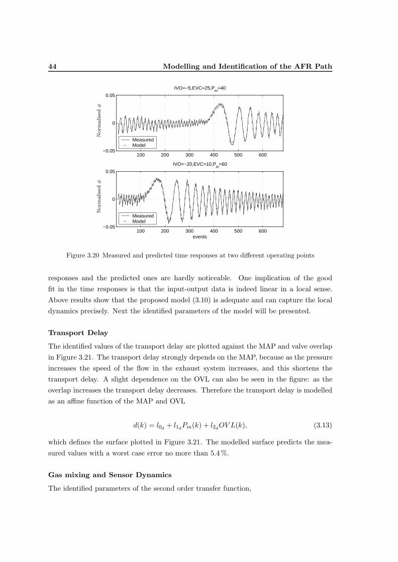
44 Modelling and Identification of the AFR Path
100 200 300 400 500 600−0.05
0
0.05
IVO=−5,EVC=25,Pm
=40
MeasuredModel
100 200 300 400 500 600−0.05
0
0.05
events
IVO=−20,EVC=10,Pm
=60
MeasuredModel
Norm
ali
sedφ
Norm
ali
sedφ
Figure 3.20 Measured and predicted time responses at two different operating points
responses and the predicted ones are hardly noticeable. One implication of the goodfit in the time responses is that the input-output data is indeed linear in a local sense.Above results show that the proposed model (3.10) is adequate and can capture the localdynamics precisely. Next the identified parameters of the model will be presented.
Transport Delay
The identified values of the transport delay are plotted against the MAP and valve overlapin Figure 3.21. The transport delay strongly depends on the MAP, because as the pressureincreases the speed of the flow in the exhaust system increases, and this shortens thetransport delay. A slight dependence on the OVL can also be seen in the figure: as theoverlap increases the transport delay decreases. Therefore the transport delay is modelledas an affine function of the MAP and OVL
d(k) = l0d + l1dPm(k) + l2dOV L(k), (3.13)
which defines the surface plotted in Figure 3.21. The modelled surface predicts the mea-sured values with a worst case error no more than 5.4 %.
Gas mixing and Sensor Dynamics
The identified parameters of the second order transfer function,

3.2. Fuel Path Dynamics 45
3035
4045
5055
600
10
20
30
404.5
5
5.5
6
6.5
Worst case error is 5.4%
ActualFit
Pm (kPa)
Del
ay(e
ven
ts)
OV L (degrees)
Figure 3.21 Variation of the transport delay with valve overlap and manifold pressure
Gx(z) =1 + ξ1 + ξ2
z2 + ξ1z + ξ2
describing the gas mixing and sensor dynamics are presented in Figure 3.22 and Fig-ure 3.23. The identified parameters ξ1 and ξ2 are modelled as affine functions of the MAPand OVL
ξ1 = l10x + l11xPm(k) + l12xOV L(k),
ξ2 = l20x + l21xPm(k) + l22xOV L(k). (3.14)
The significance of the variations in the parameters can be interpreted by analysing thechange in the pole locations of Gx(·) with respect to the MAP and OVL. The modelledsurfaces show that increasing the MAP increases ξ1 but decreases ξ2. Such a change in ξ1
and ξ2 moves the poles closer to the origin as shown in Table 3.3. This also increases thesystem gain at high frequencies because in a discrete-time system dynamics become fasteras the poles move closer to the origin. On the other hand, increasing the OVL, whichreduces the value of ξ1 but increases the value of ξ2, moves the poles closer to the unitcircle as shown in Table 3.4. This in turn reduces the system gain and increases the phaseof the system. All these predictions of the identified parameter varying model agree wellwith the highlighted trends presented in Figure 3.17.
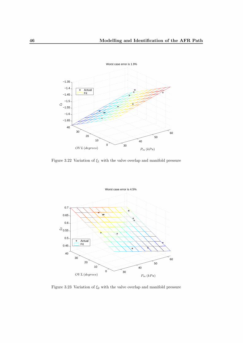
46 Modelling and Identification of the AFR Path
30
40
50
60
0
10
20
30
40
−1.65
−1.6
−1.55
−1.5
−1.45
−1.4
−1.35
Worst case error is 1.9%
ActualFit
Pm (kPa)
ξ 1
OV L (degrees)
Figure 3.22 Variation of ξ1 with the valve overlap and manifold pressure
30
40
50
60
0
10
20
30
40
0.45
0.5
0.55
0.6
0.65
0.7
Worst case error is 4.5%
ActualFit
Pm (kPa)
ξ 2
OV L (degrees)
Figure 3.23 Variation of ξ2 with the valve overlap and manifold pressure
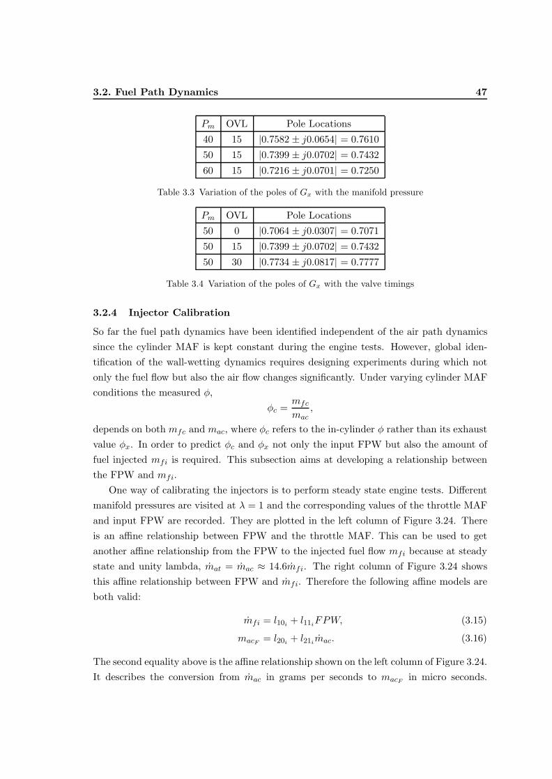
3.2. Fuel Path Dynamics 47
Pm OVL Pole Locations
40 15 |0.7582 ± j0.0654| = 0.7610
50 15 |0.7399 ± j0.0702| = 0.7432
60 15 |0.7216 ± j0.0701| = 0.7250
Table 3.3 Variation of the poles of Gx with the manifold pressure
Pm OVL Pole Locations
50 0 |0.7064 ± j0.0307| = 0.7071
50 15 |0.7399 ± j0.0702| = 0.7432
50 30 |0.7734 ± j0.0817| = 0.7777
Table 3.4 Variation of the poles of Gx with the valve timings
3.2.4 Injector Calibration
So far the fuel path dynamics have been identified independent of the air path dynamicssince the cylinder MAF is kept constant during the engine tests. However, global iden-tification of the wall-wetting dynamics requires designing experiments during which notonly the fuel flow but also the air flow changes significantly. Under varying cylinder MAFconditions the measured φ,
φc =mfc
mac,
depends on both mfc and mac, where φc refers to the in-cylinder φ rather than its exhaustvalue φx. In order to predict φc and φx not only the input FPW but also the amount offuel injected mfi is required. This subsection aims at developing a relationship betweenthe FPW and mfi.
One way of calibrating the injectors is to perform steady state engine tests. Differentmanifold pressures are visited at λ = 1 and the corresponding values of the throttle MAFand input FPW are recorded. They are plotted in the left column of Figure 3.24. Thereis an affine relationship between FPW and the throttle MAF. This can be used to getanother affine relationship from the FPW to the injected fuel flow mfi because at steadystate and unity lambda, mat = mac ≈ 14.6mfi. The right column of Figure 3.24 showsthis affine relationship between FPW and mfi. Therefore the following affine models areboth valid:
mfi = l10i + l11iFPW, (3.15)
macF = l20i + l21imac. (3.16)
The second equality above is the affine relationship shown on the left column of Figure 3.24.It describes the conversion from mac in grams per seconds to macF in micro seconds.

48 Modelling and Identification of the AFR Path
10 12 14 16 18
3500
4000
4500
5000
5500
6000
6500ActualFit
4000 5000 6000
0.6
0.7
0.8
0.9
1
1.1
1.2
ActualFit
FPW (µs)
FPW
(µs)
mat (g/s)
mfi(g/s)
Figure 3.24 Injector calibration data
Both of these conversions are valid for the calibration of the injectors since AFR is adimensionless number. In the rest of this thesis macF will be used in order to calculateestimates of φ or λ.
3.2.5 Wall-Wetting Dynamics
The calibration of the injectors completes the identification of the AFR path model apartfrom the wall-wetting dynamics. It has already been shown in (3.11) that the variation ofthe fuel puddle mass with VCT can be modelled if the relative variation of X and τ withrespect to each other can be identified during the VCT transients.
Recall that X and τ parameters of the slow and fast fuel puddles have already beenidentified for different valve timings in Section 3.2.3 as they are part of the parameter vectorΘ in optimisation (3.12). Unfortunately, the interpolation of the wall-wetting parametersobtained by the local linear identification method fails to predict the variations in thefuel film mass, even though the models predict the local linear behaviour very well, asshown in Figures 3.19 and 3.20. Therefore, a global identification scheme is proposed inthe following to model the wall-wetting dynamics and variations in the fuel film mass.
The proposed framework for the global identification scheme is depicted in Figure 3.25,in which the complete AFR path model is used. The inputs to the model are the FPW,IVO, EVC and MAP, and the output is the equivalence ratio at the exhaust measured bythe lambda sensor. Once the appropriate input-output data are collected, the nonlinear

3.2. Fuel Path Dynamics 49
ddt
Cylinder
MAF
Injection
Delay Wall Wetting
Transport Delay
Gas Mixingand Sensor
OPTIMISATION
ROUTINE
AFR PATH MODEL
mfc
macF
φc φx
φx
×÷
+
−
Θ
Pm
FPW
EV C
IV O
Figure 3.25 Global identification framework for wall-wetting dynamics
optimisation routine calculates the parameters of the wall-wetting model to minimise theidentification cost (recall that the rest of the model have already been identified). Theparameterisation of the wall-wetting transfer function
Gww(z) =(
Xsτsz − (1− τs)
+Xf τf
z − (1− τf )+ 1−Xs −Xf
)has to be determined in order to proceed with the identification process. After a few trialsthe following parameterisation, which is inspired by the empirical data, is found to besatisfactory
τs = l10s + l11sPm
Xs = l20s + l21sPm
τf = l10f + l12fEV C + l13f IV O
Xf = l20f + l22fEV C + l23f IV O (3.17)
Since it has been observed that there is a fast variation in the fuel film mass with the valvetimings not with the manifold pressure, the fast fuel puddle parameters are modelled asfunctions of EVC and IVO. On the other hand, since no such variations are observed forthe slow fuel puddle under VCT transients, its parameters are modelled as functions ofthe manifold pressure instead. This is because the manifold pressure is an indicator of theengine load and known to affect the fuel film evaporation rate.
The global identification framework is implemented in MATLAB/Simulink environ-ment, which requires realisation of the parameter-varying transfer functions Gww(z) and
50 Modelling and Identification of the AFR Path
Gx(z) in the state-space form. The next subsection discusses the details of how a reali-sation of a parameter-varying transfer function may affect the input-output behaviour ofthe system.
State-Space Realisation of the Parameter-Varying Transfer Functions
There are two parameter-varying (PV) transfer functions in the AFR path model. ThePV wall-wetting model is to be identified and the PV gas mixing and sensor model hasalready been identified. During this study it is noticed that a PV system has an interestingproperty due its time-varying nature, i.e. the ability to change its output even if the inputexcitation is constant. This property is useful and desirable in the case of modelling thewall-wetting dynamics, for which the fuel flow out of the film changes even if the injectedfuel is constant due to the varying valve timings. However, such a change of the outputvalue when the input signal is constant is not desirable for the gas mixing and sensordynamics. The underlying principles of the system and observations show that the sensoroutput signal should only change when the input signal changes, or at least this is thedesired operation of the sensor. Therefore care has to be taken when obtaining a state-space realisation of the gas mixing and sensor model. The following realisation of Gx(z)satisfy the desired properties, i.e. its output only changes when the input changes.
Gx(z) =1 + ξ1 + ξ2
z2 + ξ1z + ξ2
=
[Ax(ξ) Bx(ξ)
Cx 0
]
=
0 1 0−ξ2 −ξ1 1 + ξ1 + ξ2
1 0 0
. (3.18)
This can be seen by the fact that the matrix product (I −Ax(ξ))−1Bx(ξ) and the steadystate output Yss
Yss = Cx(I −Ax(ξ))−1Bx(ξ)Uss
are independent of ξ.On the other hand, the wall-wetting transfer function can be realised as
Gww(z) =
1− τs 0 Xs0 1− τf Xfτs τf 1−Xs −Xf
, (3.19)
where the states of the realisation represent the fuel film masses. Furthermore, for a4-cylinder engine with identical wall-wetting dynamics at each port, the state-space reali-sation with the multiplexing effect takes the form
3.2. Fuel Path Dynamics 51
Gww(z) =
0 1− τs 0 0 XsI3 0 0 0 00 0 0 1− τf Xf0 0 I3 0 0
0 τs 0 τf 1−Xs −Xf
. (3.20)
In this realisation the states 1 through 4 represent the four slow fuel puddle masses and thestates 5 through 8 represent the four fast fuel puddle masses. Both the single or 4-cylinderstate-space realisations have their outputs mfc changing under the parameter variationseven if the input fuel flow is constant.
Identification Algorithm
The natural error for the identification scheme may be the difference between the actualequivalence ratio and the predicted equivalence ratio, yet such a choice tries to optimisethe steady state accuracy as well as the transient accuracy. Since the transient accuracyis what is required to model the fast fuel film variations under rapid VCT disturbances,the error is defined as the derivative of the difference between the actual equivalence ratioand the predicted equivalence ratio. Hence the identification cost can be written as
εT ε =[d
dt(φx− φ
x)]T [ d
dt(φx− φ
x)]
(3.21)
where φx
is the measured equivalence ratio vector, φx
is the predicted equivalence ratiovector and d
dt is the derivative operator in the event based discrete-time domain.It is important that the identified dynamics are stable. This can be assured by putting
simple constraints on the poles of Gww(z) such as
|1− τs| < 1 and |1− τf | < 1.
However, the locations of the zeros of the wall-wetting model are also very important. Theidentified PV wall-wetting model must be invertible, i.e. all of its zeros must be inside theunit circle in z-domain, since the feedforward controller design for the AFR control usuallyinvolves inverting the wall-wetting transfer function. The zeros of Gww(z) are given bythe roots of the following quadratic in z
Nww(z) =(1−Xs −Xf )z2 + [−2(1−Xs −Xf ) + τs(1−Xf ) + τf (1−Xs)] z+ [(1−Xs −Xf )− τs(1−Xf )− τf (1−Xs) + τsτf ] (3.22)
The root locations of this quadratic in z-domain can be checked by Jury’s stabilitytest [Oga87], which states that for a quadratic of the form
N(z) = n0z2 + n1z + n2
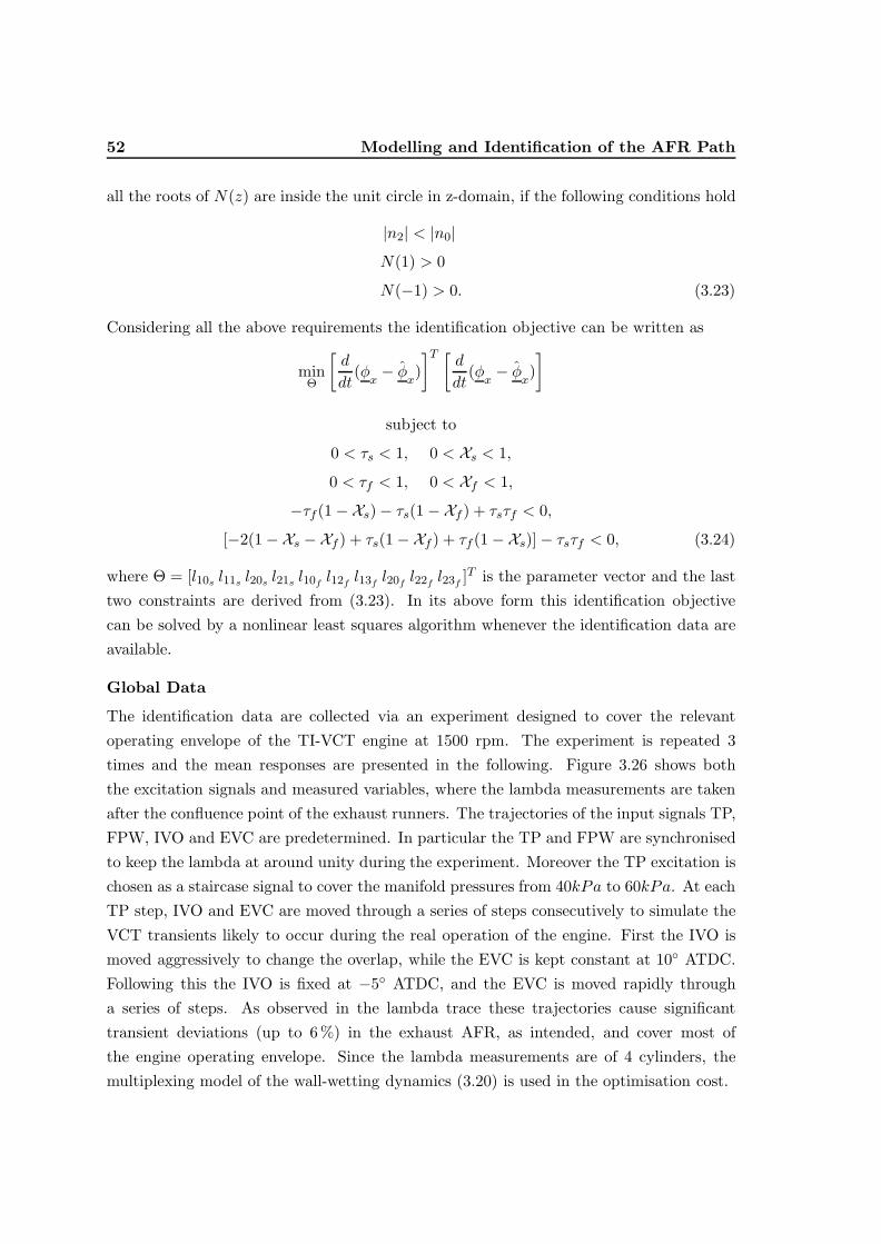
52 Modelling and Identification of the AFR Path
all the roots of N(z) are inside the unit circle in z-domain, if the following conditions hold
|n2| < |n0|N(1) > 0
N(−1) > 0. (3.23)
Considering all the above requirements the identification objective can be written as
minΘ
[d
dt(φx− φ
x)]T [ d
dt(φx− φ
x)]
subject to
0 < τs < 1, 0 < Xs < 1,
0 < τf < 1, 0 < Xf < 1,
−τf (1−Xs)− τs(1−Xf ) + τsτf < 0,
[−2(1−Xs −Xf ) + τs(1−Xf ) + τf (1−Xs)]− τsτf < 0, (3.24)
where Θ = [l10s l11s l20s l21s l10f l12f l13f l20f l22f l23f ]T is the parameter vector and the lasttwo constraints are derived from (3.23). In its above form this identification objectivecan be solved by a nonlinear least squares algorithm whenever the identification data areavailable.
Global Data
The identification data are collected via an experiment designed to cover the relevantoperating envelope of the TI-VCT engine at 1500 rpm. The experiment is repeated 3times and the mean responses are presented in the following. Figure 3.26 shows boththe excitation signals and measured variables, where the lambda measurements are takenafter the confluence point of the exhaust runners. The trajectories of the input signals TP,FPW, IVO and EVC are predetermined. In particular the TP and FPW are synchronisedto keep the lambda at around unity during the experiment. Moreover the TP excitation ischosen as a staircase signal to cover the manifold pressures from 40kPa to 60kPa. At eachTP step, IVO and EVC are moved through a series of steps consecutively to simulate theVCT transients likely to occur during the real operation of the engine. First the IVO ismoved aggressively to change the overlap, while the EVC is kept constant at 10◦ ATDC.Following this the IVO is fixed at −5◦ ATDC, and the EVC is moved rapidly througha series of steps. As observed in the lambda trace these trajectories cause significanttransient deviations (up to 6 %) in the exhaust AFR, as intended, and cover most ofthe engine operating envelope. Since the lambda measurements are of 4 cylinders, themultiplexing model of the wall-wetting dynamics (3.20) is used in the optimisation cost.
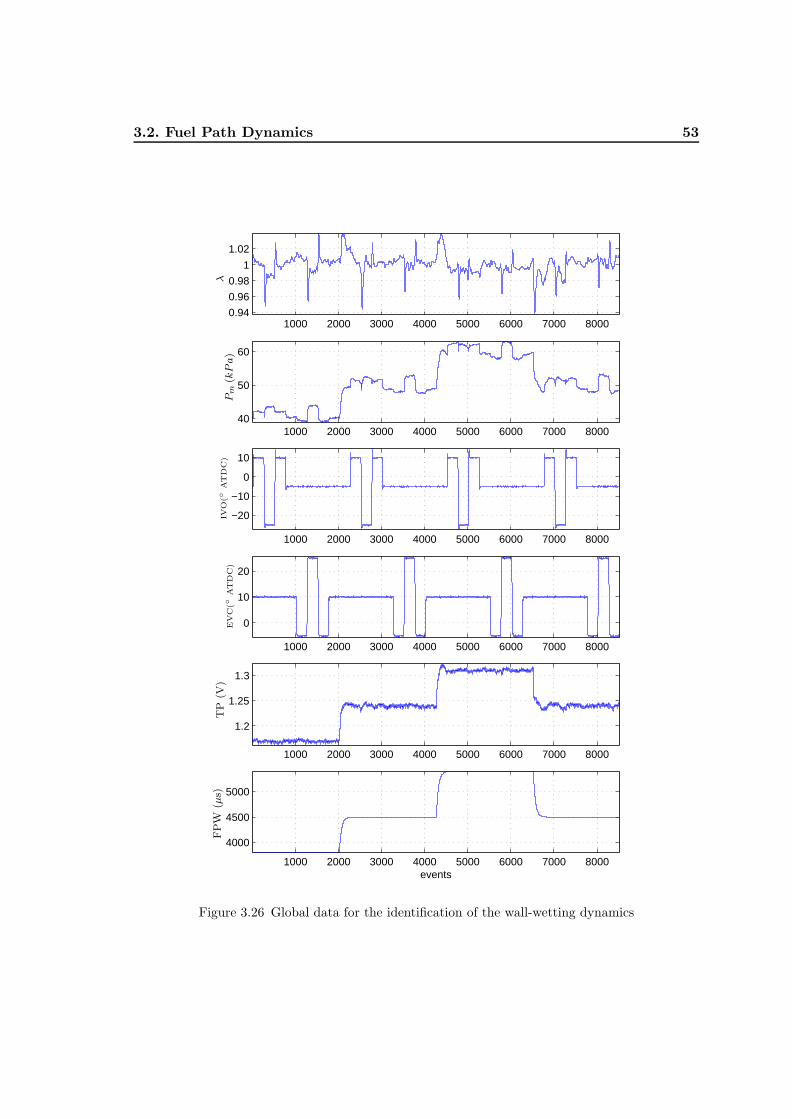
3.2. Fuel Path Dynamics 53
1000 2000 3000 4000 5000 6000 7000 80000.94
0.96
0.98
1
1.02
1000 2000 3000 4000 5000 6000 7000 800040
50
60
1000 2000 3000 4000 5000 6000 7000 8000
−20
−10
0
10
1000 2000 3000 4000 5000 6000 7000 8000
0
10
20
1000 2000 3000 4000 5000 6000 7000 8000
1.2
1.25
1.3
1000 2000 3000 4000 5000 6000 7000 8000
4000
4500
5000
events
Pm
(kPa)
λF
PW
(µs)
IVO
(◦A
TD
C)
EV
C(◦
AT
DC
)T
P(V
)
Figure 3.26 Global data for the identification of the wall-wetting dynamics
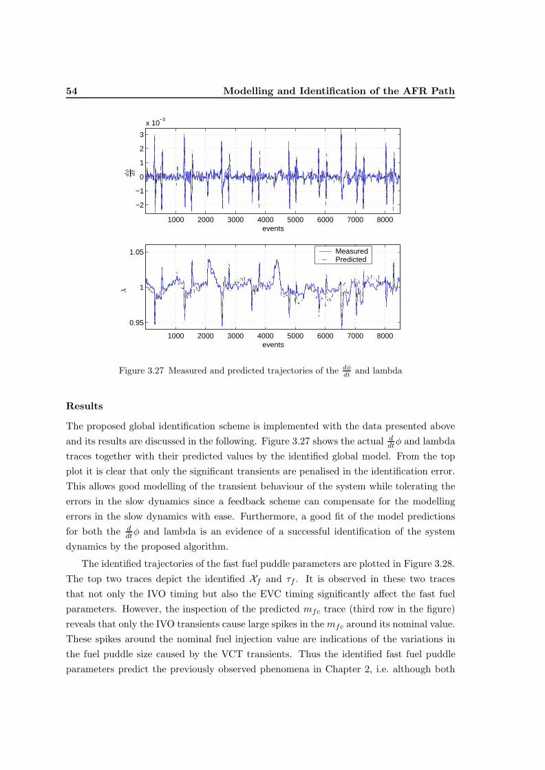
54 Modelling and Identification of the AFR Path
1000 2000 3000 4000 5000 6000 7000 8000
−2
−1
0
1
2
3
x 10−3
events
1000 2000 3000 4000 5000 6000 7000 8000
0.95
1
1.05
events
Measured Predicted
λdφdt
Figure 3.27 Measured and predicted trajectories of the dφdt and lambda
Results
The proposed global identification scheme is implemented with the data presented aboveand its results are discussed in the following. Figure 3.27 shows the actual d
dtφ and lambdatraces together with their predicted values by the identified global model. From the topplot it is clear that only the significant transients are penalised in the identification error.This allows good modelling of the transient behaviour of the system while tolerating theerrors in the slow dynamics since a feedback scheme can compensate for the modellingerrors in the slow dynamics with ease. Furthermore, a good fit of the model predictionsfor both the d
dtφ and lambda is an evidence of a successful identification of the systemdynamics by the proposed algorithm.
The identified trajectories of the fast fuel puddle parameters are plotted in Figure 3.28.The top two traces depict the identified Xf and τf . It is observed in these two tracesthat not only the IVO timing but also the EVC timing significantly affect the fast fuelparameters. However, the inspection of the predicted mfc trace (third row in the figure)reveals that only the IVO transients cause large spikes in the mfc around its nominal value.These spikes around the nominal fuel injection value are indications of the variations inthe fuel puddle size caused by the VCT transients. Thus the identified fast fuel puddleparameters predict the previously observed phenomena in Chapter 2, i.e. although both

3.2. Fuel Path Dynamics 55
1000 2000 3000 4000 5000 6000 7000 8000
0.3
0.35
0.4
0.45
1000 2000 3000 4000 5000 6000 7000 8000
0.4
0.5
0.6
0.7
1000 2000 3000 4000 5000 6000 7000 8000
4000
4500
5000
5500
1000 2000 3000 4000 5000 6000 7000 8000
−20
−10
0
10
1000 2000 3000 4000 5000 6000 7000 8000
0
10
20
events
τ fXf
mfc
(µs)
IVO
(◦ATDC
)EVC
(◦ATDC
)
Figure 3.28 Identified trajectories of the fast fuel puddle parameters

56 Modelling and Identification of the AFR Path
IVO and EVC transients cause AFR deviations, only the IVO transients have a significanteffect on the fuel film size. Note that there are also some tiny spikes caused by the EVCin the mfc trace, yet they are almost negligible compare to the IVO induced spikes.
The identified parameter surfaces of the fast fuel puddle are given in Figures 3.29and 3.30, which expose the variations in Xf and τf with respect to the valve timings.Both parameter surfaces have the same trends: retarding the EVC makes the parameterssmaller, whereas advancing the IVO makes the parameters larger.
The above results are very convincing in the sense that the identified model can capturethe observed fast fuel puddle dynamics, but it is not yet clear why only the parametervariations caused by IVO change the mfc in the model. The answer to this question ishidden in (3.11), which suggests that the fuel puddle mass is proportional to Xfτf at steadystate. This ratio is plotted in Figure 3.31 for further investigation. The large variations inthe Xfτf are seen under the IVO excitation but the variations under the EVC excitation aremuch smaller. This explains why the IVO excitation causes significant transients in thepredicted mfc trace. Moreover, Figure 3.31 hints that the identified model captures thevariations in the fuel film size by shaping the Xfτf ratio rather than the individual values
of Xf and τf . The relationship between the Xfτf and fuel film size is further evident when
the mfc trace in Figure 3.28 is compared with the Xfτf trace in Figure 3.31. It shows that
any positive (negative) step in the Xfτf cause a negative (positive) spike in the mfc traceas expected.
The identified trajectories of the slow fuel puddle parameters are shown in Figure 3.32.It shows that the parameter variations in the slow fuel puddle model are much smaller thanthe parameter variations in the fast fuel puddle model. Although the slow fuel parametersare inversely proportional with the manifold pressure, they do not affect the mfc, but tinydeviations in mfc can be seen at high loads around event 6000.
The identified values of the Xs and τs with respect to the manifold pressure are plottedin Figure 3.33. It shows that both parameters are inversely proportional with MAP. Theinverse proportionality of the evaporation constant with the MAP agrees with the physicalfact that the evaporation is helped by lower pressures [SLOG00].
Finally, the zeros of the identified PV wall-wetting transfer function (of a single cylin-der) are plotted in Figure 3.34. The zeros of the PV transfer function always stay in theunit circle as constrained by the optimisation scheme. This ensures that the PV transferfunction remains invertible over all of the operating envelope. Therefore a feedforwardcontrol scheme can easily be designed by inverting the identified PV wall-wetting model.
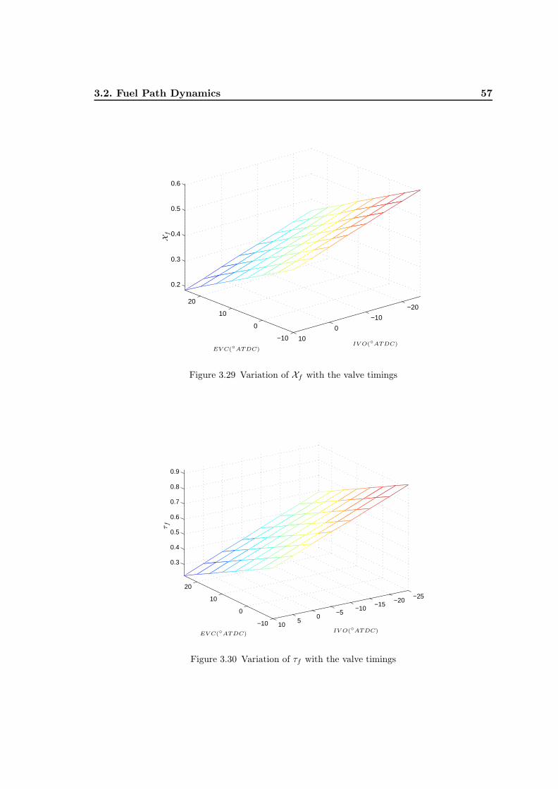
3.2. Fuel Path Dynamics 57
−10
0
10
20−20
−10
0
10
0.2
0.3
0.4
0.5
0.6
Xf
IV O(◦ATDC)EVC(◦ATDC)
Figure 3.29 Variation of Xf with the valve timings
−10
0
10
20
−25−20
−15−10
−50
510
0.3
0.4
0.5
0.6
0.7
0.8
0.9
τ f
IV O(◦ATDC)EVC(◦ATDC)
Figure 3.30 Variation of τf with the valve timings
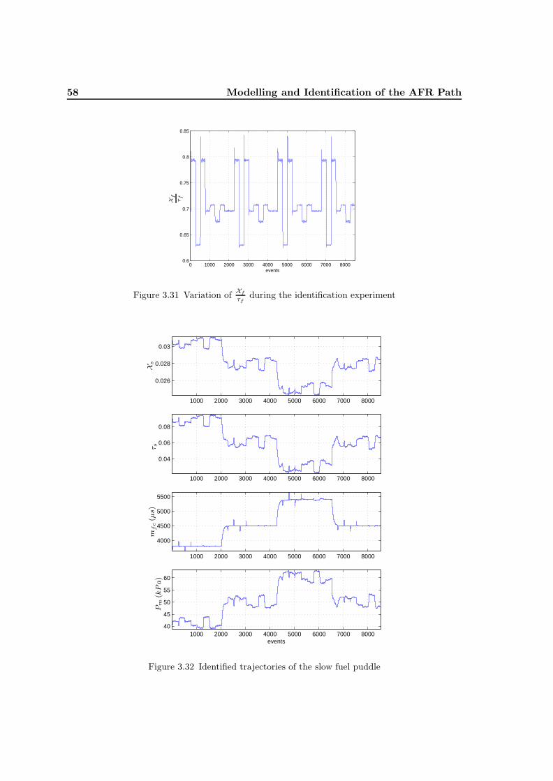
58 Modelling and Identification of the AFR Path
0 1000 2000 3000 4000 5000 6000 7000 80000.6
0.65
0.7
0.75
0.8
0.85
events
Xf
τf
Figure 3.31 Variation of Xfτf during the identification experiment
1000 2000 3000 4000 5000 6000 7000 8000
0.026
0.028
0.03
1000 2000 3000 4000 5000 6000 7000 8000
0.04
0.06
0.08
1000 2000 3000 4000 5000 6000 7000 8000
4000
4500
5000
5500
1000 2000 3000 4000 5000 6000 7000 800040
45
50
55
60
events
τ sXs
Pm
(kPa)
mfc
(µs)
Figure 3.32 Identified trajectories of the slow fuel puddle

3.2. Fuel Path Dynamics 59
35 40 45 50 55 60 650.024
0.026
0.028
0.03
0.032
35 40 45 50 55 60 650.02
0.04
0.06
0.08
0.1
τ sXs
Pm (kPa)
Pm (kPa)
Figure 3.33 Variation of Xs and τs with the manifold pressure
−1 −0.8 −0.6 −0.4 −0.2 0 0.2 0.4 0.6 0.8 1−1
−0.8
−0.6
−0.4
−0.2
0
0.2
0.4
0.6
0.8
1
Imag
Real
Zeros
Figure 3.34 Zeros of Gww(z)
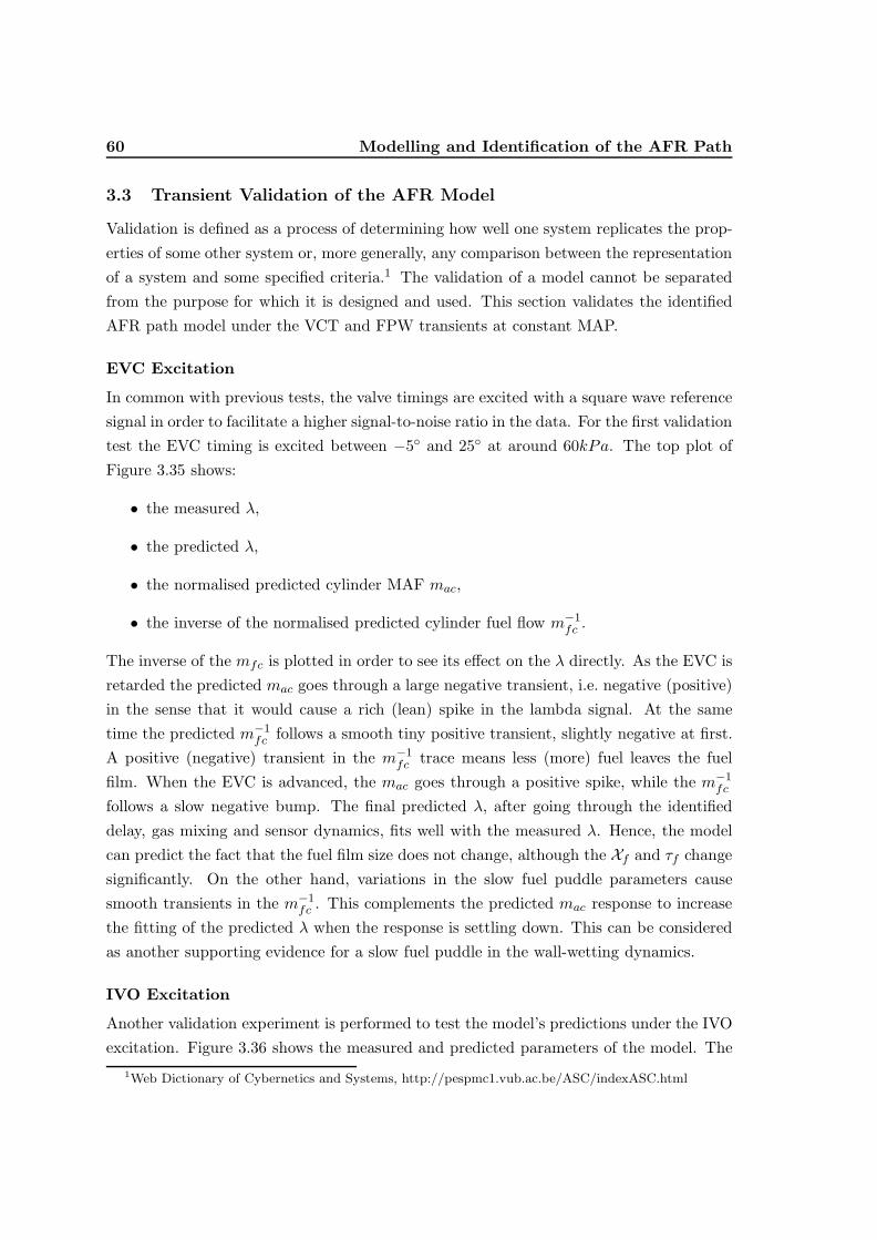
60 Modelling and Identification of the AFR Path
3.3 Transient Validation of the AFR Model
Validation is defined as a process of determining how well one system replicates the prop-erties of some other system or, more generally, any comparison between the representationof a system and some specified criteria.1 The validation of a model cannot be separatedfrom the purpose for which it is designed and used. This section validates the identifiedAFR path model under the VCT and FPW transients at constant MAP.
EVC Excitation
In common with previous tests, the valve timings are excited with a square wave referencesignal in order to facilitate a higher signal-to-noise ratio in the data. For the first validationtest the EVC timing is excited between −5◦ and 25◦ at around 60kPa. The top plot ofFigure 3.35 shows:
• the measured λ,
• the predicted λ,
• the normalised predicted cylinder MAF mac,
• the inverse of the normalised predicted cylinder fuel flow m−1fc .
The inverse of the mfc is plotted in order to see its effect on the λ directly. As the EVC isretarded the predicted mac goes through a large negative transient, i.e. negative (positive)in the sense that it would cause a rich (lean) spike in the lambda signal. At the sametime the predicted m−1
fc follows a smooth tiny positive transient, slightly negative at first.A positive (negative) transient in the m−1
fc trace means less (more) fuel leaves the fuelfilm. When the EVC is advanced, the mac goes through a positive spike, while the m−1
fc
follows a slow negative bump. The final predicted λ, after going through the identifieddelay, gas mixing and sensor dynamics, fits well with the measured λ. Hence, the modelcan predict the fact that the fuel film size does not change, although the Xf and τf changesignificantly. On the other hand, variations in the slow fuel puddle parameters causesmooth transients in the m−1
fc . This complements the predicted mac response to increasethe fitting of the predicted λ when the response is settling down. This can be consideredas another supporting evidence for a slow fuel puddle in the wall-wetting dynamics.
IVO Excitation
Another validation experiment is performed to test the model’s predictions under the IVOexcitation. Figure 3.36 shows the measured and predicted parameters of the model. The
1Web Dictionary of Cybernetics and Systems, http://pespmc1.vub.ac.be/ASC/indexASC.html

3.3. Transient Validation of the AFR Model 61
50 100 150 200 250 300 350 400 450
0.96
0.97
0.98
0.99
1
1.01
1.02
1.03
1.04
events
100 200 300 400
60
61
62
63
100 200 300 400
0
10
20
100 200 300 400
0.3
0.35
0.4
0.45
100 200 300 400
0.4
0.5
0.6
100 200 300 4000.024
0.0245
0.025
events100 200 300 400
0.02
0.025
0.03
events
τ sXs
Pm
(kPa)
τ fXf
EVC
(◦ATDC
)λ
Measured λPredicted λPredicted macPredicted m−1
fc
Figure 3.35 Transient validation of the AFR path model (EVC excitation)
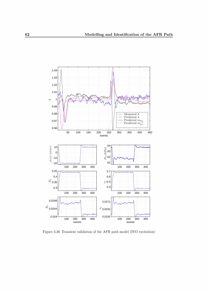
62 Modelling and Identification of the AFR Path
50 100 150 200 250 300 350 400 450
0.96
0.97
0.98
0.99
1
1.01
1.02
1.03
1.04
events
100 200 300 400
61
62
63
64
100 200 300 400−20
−10
0
10
100 200 300 400
0.3
0.35
0.4
0.45
100 200 300 400
0.4
0.5
0.6
0.7
100 200 300 4000.024
0.0244
0.0248
events100 200 300 400
0.0191
0.0231
0.0271
events
τ sXs
Pm
(kPa)
τ fXf
IVO
(◦ATDC
)λ
Measured λPredicted λPredicted macPredicted m−1
fc
Figure 3.36 Transient validation of the AFR path model (IVO excitation)

3.4. Comments 63
IVO timing is changed between 10◦ and −20◦ in a square wave manner. This causesfirst a positive and then a negative (positive-negative) spike in the mac, while the m−1
fc
goes through a large single negative transient. The combined effect is that the negativem−1fc spike cancels the positive mac spike and causes a rich λ transient. This matches
the measured λ accurately. When the IVO is retarded the mac goes through a positive-negative transient, while the m−1
fc follows a single lean spike. It can be seen that the finalpredicted λ accurately models the actual λ. All the fuel transients in the model are due tothe changes in the fast fuel puddle parameters. Moreover, the slow fuel puddle parametersdo not change much since the variations in the MAP are small under the IVO excitation.
FPW Excitation
The final validation test is performed under a FPW excitation, where the injected fuel ischanged in a square wave form. The average responses and model predictions are plottedin Figure 3.37. Since during this test all the input excitations apart from the FPW areconstant, the wall-wetting dynamics are almost frozen as the predicted values of the fuelpuddle parameters indicate. The high frequency engine induced noise can be seen in themeasurements. The slow oscillation present in the normalised predicted mac around itsnominal value is due to the oscillation in the MAP trace. The measured λ is predictedwell by the model during the FPW excitation and this confirms that the model can alsosatisfactorily capture the frozen (linear) dynamics of the AFR path.
3.4 Comments
The AFR path of a TI-VCT engine is modelled and identified in this chapter by mostlyfollowing conventional methods. The two main contributions of the chapter are:
i. A new formulation for the cylinder MAF in a TI-VCT engine is proposed and val-idated in Section 3.1.2. The new formulation has a more intuitive form than thestandard regression form.
ii. A global identification scheme that can capture the nonlinear behaviour of the systemis proposed for the identification of the wall-wetting dynamics. Furthermore, aparameter-varying wall-wetting model for a TI-VCT engine has been identified usingthe proposed scheme and partially validated in Section 3.2.5 and Section 3.3 for thefirst time to author’s knowledge as far as the published literature is concerned. Thisis an improvement on the widely accepted local linear identification methods.
Since the identified model is a parameter-varying one, it might be interesting to see howwell the recently developed linear parameter-varying identification methods would per-form on the TI-VCT engine [LP96, MMP99]. In addition to the AFR path dynamics,

64 Modelling and Identification of the AFR Path
50 100 150 200 250 300 350 400 450
0.98
0.99
1
1.01
1.02
1.03
1.04
events
100 200 300 40060
61
62
100 200 300 4005400
5500
5600
5700
100 200 300 4000.455
0.46
0.465
0.47
100 200 300 4000.725
0.73
0.735
0.74
0.745
100 200 300 4000.0247
0.0248
0.0249
0.025
events100 200 300 400
0.026
0.027
0.028
0.029
events
τ sXs
Pm
(kPa)
τ fXf
FP
W(µ
s)λ
Measured λPredicted λPredicted macPredicted m−1
fc
Figure 3.37 Transient validation of the AFR path model (FPW excitation)

3.4. Comments 65
VCT actuators’ dynamics also play an important role in the AFR control problem. Themodelling and identification of the TI-VCT actuators has been published in [GGF01].

4
LFT Representation of the AFR Path Model
Linear fractional transformations play an important role in the control theory by providinga framework that unifies many interesting and challenging control problems. SupposeP ∈ C(p1+p2)×(q1+q2) is a complex matrix partitioned as
P =
[P11 P12
P21 P22
], (4.1)
with P11 ∈ Cp1×q1 and P22 ∈ Cp2×q2 . Then, given Ql ∈ Cq2×p2 and Qu ∈ Cq1×p1,
• the lower linear fractional transformation (LFT) is defined by
Fl (P,Ql) := P11 + P12Ql(I − P22Ql)−1P21, (4.2)
• the upper LFT is defined by
Fu (P,Qu) := P22 + P21Qu(I − P11Qu)−1P12, (4.3)
provided that the required inverses exist. The motivation for the terminologies “lower”and “upper” LFTs should be clear from the diagram representations of Fl (P,Ql) andFu (P,Qu) given in Figure 4.1. Interconnections of LFTs are again LFTs. This is afundamental property of LFTs and is one reason why they are so important in the controltheory. Details of the algebraic properties of LFTs can be found in [DPZ91] and [ZDG96].
General affine state space uncertainty is a special class of state space modelswith unknown coefficients. In the following we will show how this type of uncertainty canbe represented via the LFT formulae with respect to an uncertain parameter matrix sothat perturbations enter the system in a feedback form. Consider a linear system that is
67
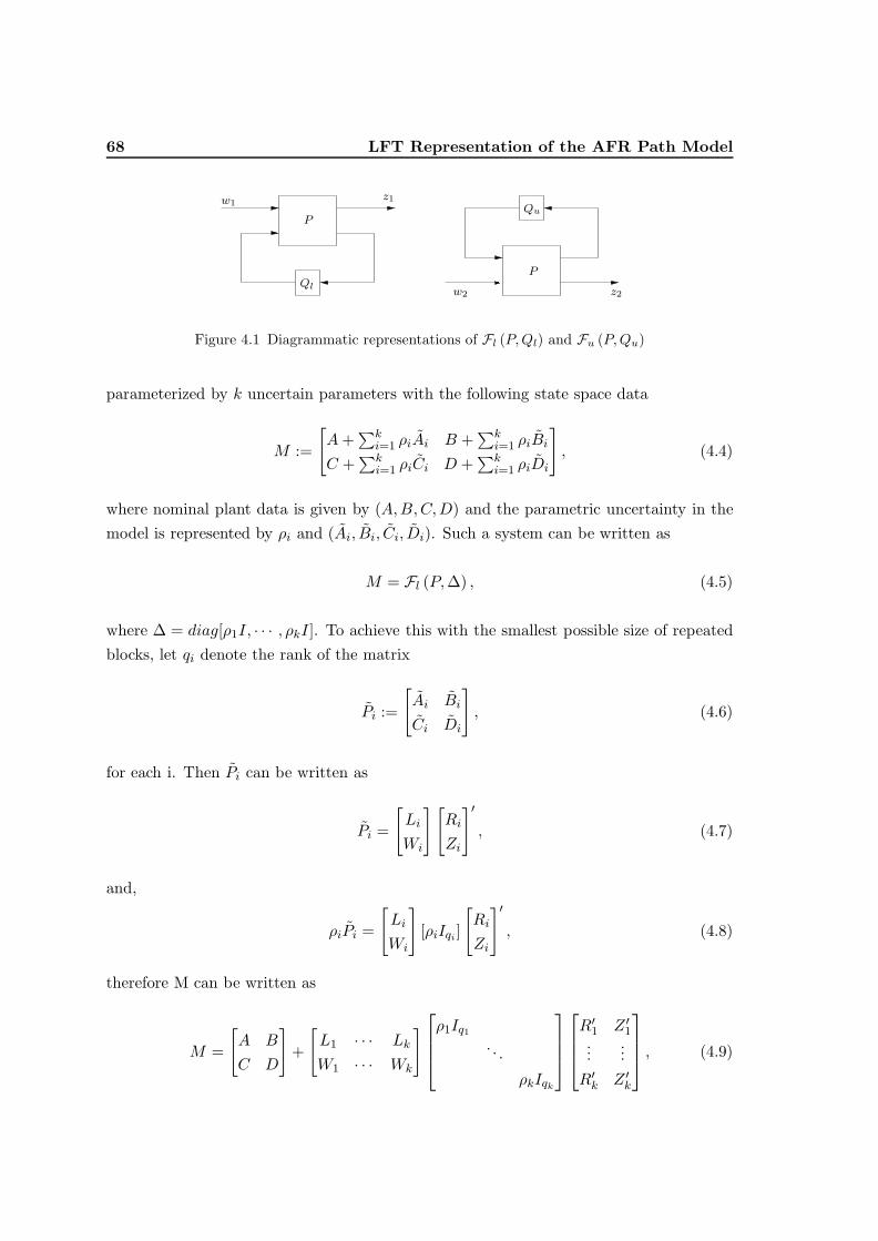
68 LFT Representation of the AFR Path Model
P
P
Ql
Quz1w1
z2w2
Figure 4.1 Diagrammatic representations of Fl (P,Ql) and Fu (P,Qu)
parameterized by k uncertain parameters with the following state space data
M :=
[A+
∑ki=1 ρiAi B +
∑ki=1 ρiBi
C +∑k
i=1 ρiCi D +∑k
i=1 ρiDi
], (4.4)
where nominal plant data is given by (A,B,C,D) and the parametric uncertainty in themodel is represented by ρi and (Ai, Bi, Ci, Di). Such a system can be written as
M = Fl (P,∆) , (4.5)
where ∆ = diag[ρ1I, · · · , ρkI]. To achieve this with the smallest possible size of repeatedblocks, let qi denote the rank of the matrix
Pi :=
[Ai Bi
Ci Di
], (4.6)
for each i. Then Pi can be written as
Pi =
[Li
Wi
] [Ri
Zi
]′, (4.7)
and,
ρiPi =
[Li
Wi
][ρiIqi ]
[Ri
Zi
]′, (4.8)
therefore M can be written as
M =
[A B
C D
]+
[L1 · · · Lk
W1 · · · Wk
]ρ1Iq1
. . .
ρkIqk
R′1 Z ′1...
...R′k Z ′k
, (4.9)
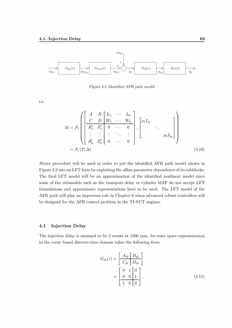
4.1. Injection Delay 69
Gdi(z) Gww(z) Gd(z) Gx(z)mfi mfid mfc
mac
φc φcd φx
×÷
Figure 4.2 Identified AFR path model
i.e.
M = Fl
A B L1 · · · Lk
C D W1 · · · Wk
R′1 Z ′1 0 · · · 0...
......
. . ....
R′k Z ′k 0 · · · 0
,
ρ1Iq1
. . .
ρkIqk
= Fl (P,∆) (4.10)
Above procedure will be used in order to put the identified AFR path model shown inFigure 4.2 into an LFT form by exploiting the affine parameter dependence of its subblocks.The final LFT model will be an approximation of the identified nonlinear model sincesome of the submodels such as the transport delay or cylinder MAF do not accept LFTformulations and approximate representations have to be used. The LFT model of theAFR path will play an important role in Chapter 6 when advanced robust controllers willbe designed for the AFR control problem in the TI-VCT engines.
4.1 Injection Delay
The injection delay is assumed to be 2 events at 1500 rpm. Its state space representationin the event based discrete-time domain takes the following form
Gdi(z) =
[Adi Bdi
Cdi Ddi
]
=
0 1 00 0 1
1 0 0
. (4.11)
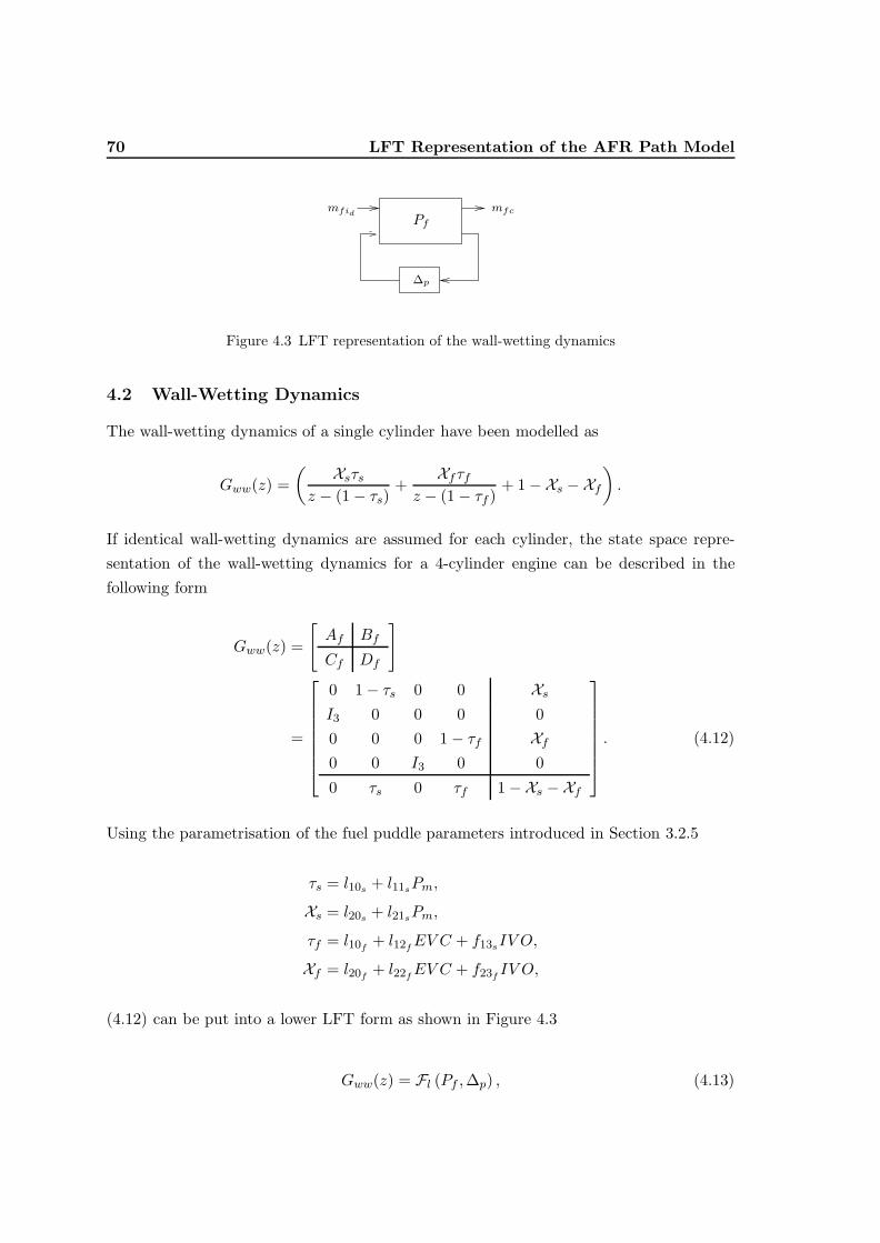
70 LFT Representation of the AFR Path Model
mfid mfcPf
∆p
Figure 4.3 LFT representation of the wall-wetting dynamics
4.2 Wall-Wetting Dynamics
The wall-wetting dynamics of a single cylinder have been modelled as
Gww(z) =(
Xsτsz − (1− τs)
+Xfτf
z − (1− τf )+ 1−Xs −Xf
).
If identical wall-wetting dynamics are assumed for each cylinder, the state space repre-sentation of the wall-wetting dynamics for a 4-cylinder engine can be described in thefollowing form
Gww(z) =
[Af Bf
Cf Df
]
=
0 1− τs 0 0 XsI3 0 0 0 00 0 0 1− τf Xf0 0 I3 0 0
0 τs 0 τf 1−Xs −Xf
. (4.12)
Using the parametrisation of the fuel puddle parameters introduced in Section 3.2.5
τs = l10s + l11sPm,
Xs = l20s + l21sPm,
τf = l10f + l12fEV C + f13sIV O,
Xf = l20f + l22fEV C + f23f IV O,
(4.12) can be put into a lower LFT form as shown in Figure 4.3
Gww(z) = Fl (Pf ,∆p) , (4.13)
4.3. Transport Delay 71
where
Pf =
0 1− l10s 0 0 l20s 1 0 0I3 0 0 0 0 0 0 00 0 0 1− l10f l20f 0 1 10 0 I3 0 0 0 0 0
0 l10s 0 l10f 1− l20s − l20f −1 −1 −10 −l11s 0 0 l21s 0 0 00 0 0 −l12f l22f 0 0 00 0 0 −l13f l23f 0 0 0
,
∆p =
Pm 0 00 EV C 00 0 IV O
.
4.3 Transport Delay
Recall that the transport delay is modelled as a delay in the event based continuous-timedomain. A time delay in the continuous-time is an infinite-dimensional system and notrepresentable by a rational transfer function. An n’th order approximation of a time delayd may be obtained by putting n first-order Pade approximations in series
e−ds ≈(1− d
2ns)n(
1 + d2ns)n . (4.14)
An equivalent approximation in the event based discrete-time domain can be calculatedvia a bilinear transformation of the form (Tustin’s transformation)
s =2Ts
1− z−1
1 + z−1. (4.15)
Substituting (4.15) into (4.14) yields the n’th order delay approximation in the discrete-time domain
e−ds ≈(nTs − d+ (nTs + d)z−1
)n(nTs + d+ (nTs − d)z−1)n
. (4.16)
Consider the case with Ts = 1 and n = 2
e−ds ≈(
2− d+ (2 + d)z−1
2 + d+ (2− d)z−1
)2
=
(2− d2 + d
z + 2+d2−d
z + 2−d2+d
).
(2− d2 + d
z + 2+d2−d
z + 2−d2+d
)(4.17)

72 LFT Representation of the AFR Path Model
If one of the terms above can be put into an LFT form, then overall expression can bewritten as an LFT since multiplication of LFTs are still LFTs. Define each term in (4.17)as
e−d′s :=
(2− d2 + d
z + 2+d2−d
z + 2−d2+d
)
= θz + θ−1
z + θ
=
[−θ 1 + θ
1− θ θ
]
= Fl
0 1 1
1 0 1−1 1 0
, θ , (4.18)
where
θ =2− d2 + d
. (4.19)
Moreover, θ also can be expressed as an LFT in d
θ = Fl
([1 − 11 − 1/2
], d
). (4.20)
Recall that the transport delay d is parameterised as
d = l0d + l1dPm + l2dOV L.
Substituting OVL=EVC−IVO, the above affine relationship also takes an LFT represen-tation
d = Fl
l0d l1d l2d −l2d1 0 0 01 0 0 01 0 0 0
,∆p
, (4.21)
Finally, LFTs (4.18), (4.20) and (4.21) can be combined to get an LFT representation ofe−d
′s in terms of Pm, EVC and IVO as depicted in Figure 4.4
e−d′s = Fl (Pd,∆p) . (4.22)

4.4. Gas Mixing and Sensor Dynamics 73
φcd′φc0 1 1
1 0 1
−1 1 0
[1 −1
1 −1/2
]
l0d l1d l2d −l2d1 0 0 0
1 0 0 0
1 0 0 0
Pd
∆p
Figure 4.4 LFT representation of e−d′s
Hence, the second order approximation of the transport delay can be written as
e−ds ≈ e−d′s.e−d′s
= Gd(z)
= Fl (Pd,∆p)Fl (Pd,∆p) (4.23)
Note that the higher order LFT approximations of the transport model can be obtainedby applying the above procedure for n > 2.
4.4 Gas Mixing and Sensor Dynamics
The identified gas mixing and sensor dynamics are modelled as a parameter-varying trans-fer function
Gx(z) =1 + ξ1 + ξ2
z2 + ξ1z + ξ2
=
[Ax Bx
Cx Dx
]
=
0 1 0−ξ2 −ξ1 1 + ξ1 + ξ2
1 0 0
, (4.24)
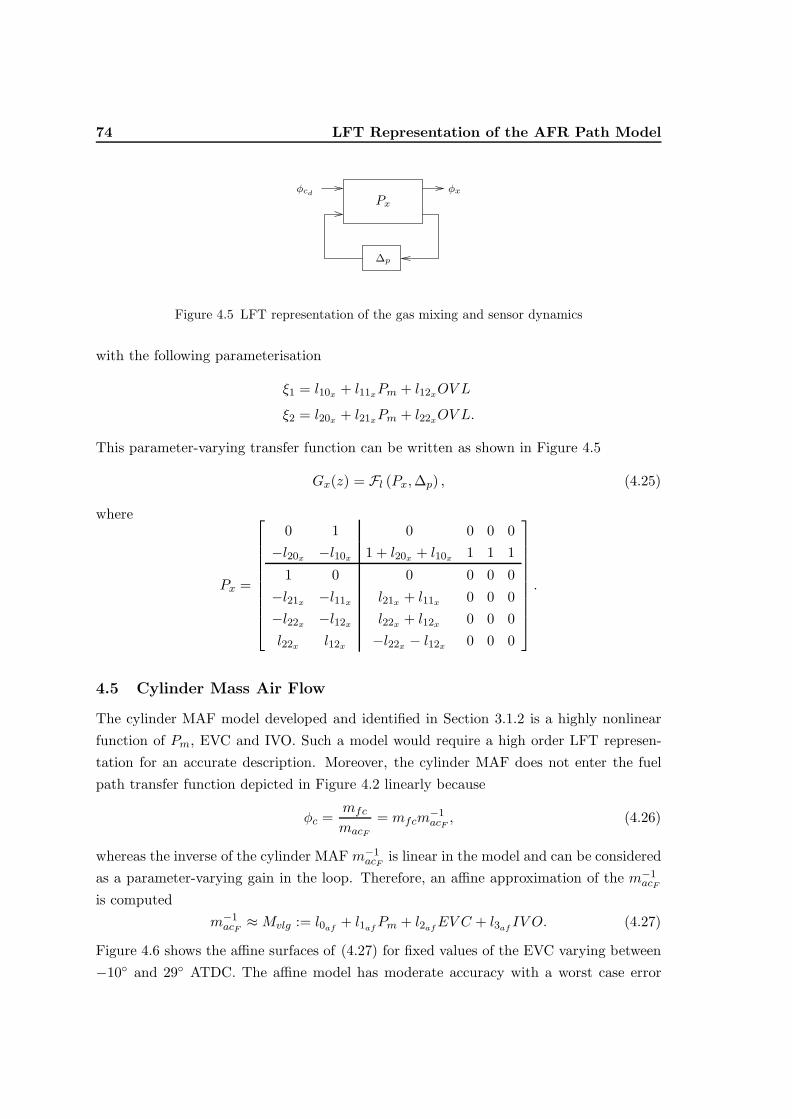
74 LFT Representation of the AFR Path Model
φcd φxPx
∆p
Figure 4.5 LFT representation of the gas mixing and sensor dynamics
with the following parameterisation
ξ1 = l10x + l11xPm + l12xOV L
ξ2 = l20x + l21xPm + l22xOV L.
This parameter-varying transfer function can be written as shown in Figure 4.5
Gx(z) = Fl (Px,∆p) , (4.25)
where
Px =
0 1 0 0 0 0−l20x −l10x 1 + l20x + l10x 1 1 1
1 0 0 0 0 0−l21x −l11x l21x + l11x 0 0 0−l22x −l12x l22x + l12x 0 0 0l22x l12x −l22x − l12x 0 0 0
.
4.5 Cylinder Mass Air Flow
The cylinder MAF model developed and identified in Section 3.1.2 is a highly nonlinearfunction of Pm, EVC and IVO. Such a model would require a high order LFT represen-tation for an accurate description. Moreover, the cylinder MAF does not enter the fuelpath transfer function depicted in Figure 4.2 linearly because
φc =mfc
macF
= mfcm−1acF
, (4.26)
whereas the inverse of the cylinder MAF m−1acF
is linear in the model and can be consideredas a parameter-varying gain in the loop. Therefore, an affine approximation of the m−1
acF
is computedm−1acF≈Mvlg := l0af + l1afPm + l2afEV C + l3af IV O. (4.27)
Figure 4.6 shows the affine surfaces of (4.27) for fixed values of the EVC varying between−10◦ and 29◦ ATDC. The affine model has moderate accuracy with a worst case error

4.6. Overall AFR Path 75
3040
5060
70
−40
−20
0
201.5
2
2.5
3
3.5
x 10−4
2920100
−10
Worst case error is 19%
m−
1acF
(µs−
1)
Pm (kPa)IV O(◦ATDC)
EVC (◦ATDC)
Figure 4.6 LFT approximation of m−1acF
no more than 19%. Note that the injector calibration data identified in Section 3.2.4 isused in order to convert the cylinder MAF output mac from ”gram per seconds” to ”microseconds” before computing the affine approximation of m−1
acF. This makes the units of the
mfc and m−1acF
compatible before the calculation of the φc in the AFR path model. Theaffine approximation of m−1
acFcan also be written in LFT form
Mvlg = Fl
l0af l1af l2af l3af1 0 0 01 0 0 01 0 0 0
,∆p
. (4.28)
Note that the LFT approximation of the cylinder air charge will be only used for feedbackcontroller synthesis, for estimation purposes and feedforward controller design the originalfull nonlinear air charge model will be used.
4.6 Overall AFR Path
Since the interconnections of the LFTs are again LFTs, the nonlinear AFR path modelcan be approximated in an LFT form by combining the individual LFT representations

76 LFT Representation of the AFR Path Model
of the transfer functions in Figure 4.2
Gφ(z) = Gx(z)Gd(z)MvlgGww(z)Gdi(z)
= Fl (Px,∆p)Fl (Pd,∆p)Fl (Pd,∆p)Fl (PM ,∆p)Fl (Pf ,∆p)Gdi
= Fl (Pφ,∆φ) , (4.29)
where Pφ ∈ R30×30 has 14 states, 16 inputs and 16 outputs, ∆φ =diag[PmI5,EVCI5,IVOI5]∈ R15×15 and Gφ is a transfer function with 14 states, 1 input and 1 output.
4.7 Comments
The identified nonlinear AFR path model has been approximated with an LFT model inthis chapter. Apart from the transport delay and inverse of the cylinder MAF, all of thesubmodels in the AFR path model identified in Chapter 3 have been exactly described inthe LFT framework. The LFT AFR path model will allow us to analyse and synthesisefeedback controllers for the AFR control problem using the powerful tools of the advancedrobust control theory introduced in Chapter 6. The loss of accuracy in the model will becompensated by designing controllers that have appropriate robustness properties. Fur-thermore, the full nonlinear AFR path model will be used in the design of a feedforwardcontroller in order to improve the performance further.
5
Robust Control System Design
This chapter introduces some concepts of the robust control theory that are necessary todesign the final AFR controller of this thesis. Preceding chapters have revealed an AFRpath model that is both uncertain and highly operating point dependent. Uncertaintyin a model is inherent and cannot be diminished. This can be seen from the validationdata provided in Section 3.3. Even though the identified model predicts the system re-sponse accurately, it cannot match it exactly. The uncertainty in a model gets even largerwhen it is used at operating points different than the operating points the identificationexperiments were performed. The inherent mismatch between a system and its model isone of the main motivations for using feedback since feedback can reduce the effect of theuncertainty on the closed-loop system. In addition to the uncertainty in the model, thedisturbances acting on the AFR signal such as the valve timings or throttle position canonly be rejected by a feedback controller. The ability to reject disturbances is anothermain motivation for using feedback control systems. The sensible design requirements fora basic feedback system are discussed in Section 5.1 in terms of stability and disturbancerejection performance. Design guidelines for the classical loop shaping framework are alsopresented in this section.
Even though mere use of the feedback improves the robustness of the closed-loopsystem, only in the robust control theory the uncertainty in the model is explicitly takeninto account during the design process. Section 5.2 introduces H∞ robust control theorytogether with the H∞ loop shaping design paradigm1. The H∞ loop shaping controllerdesign is chosen as the main controller synthesis tool in this thesis since it combines theessential ideas of the classical loop shaping with the modern ideas of robust control theoryin a convenient way. The H∞ control theory is exposed in a linear matrix inequalities(LMIs) framework as LMI techniques apply not only to standard H∞ control problems
1Details of the H∞ loop shaping design paradigm is presented in Appendix C
77

78 Robust Control System Design
but also to more difficult control problems such as the robust gain-scheduling controllerdesign.
Inherent uncertainty and multiple disturbances are not the only difficulties in theAFR control problem in TI-VCT engines. The AFR path dynamics vary significantlywith the operating point and an AFR controller has to cope with these variations withoutmuch degradation of its performance and robustness. Such variations in dynamics maybe handled in two ways. The first approach is to treat the variations as uncertainties andtechniques developed in Section 5.2 can be used. The second approach is to treat them asmeasurable parameter variations in the model and recently developed linear parameter-varying (LPV) controller design ideas can be used. Although the first option producessimple controllers, superior robustness and performance can only be achieved through thesecond option. The wide variety of techniques in LPV H∞ controller design are presentedin Section 5.3 as an extension of the LMI framework exposed in Section 5.2 in a unifiedand systematic manner as much as possible. The presentation of the LMI techniques inthis chapter closely follows the lines of [SW99,Det01].
Remark 5.1 The H∞ control theory and LPV methods introduced in this chapter are forcontinuous-time systems. They can be applied to the discrete-time systems by convertingthe discrete-time parameters to continuous-time parameters through a mapping such asthe Tustin’s (bilinear) transformation. Once the controller design is completed in thecontinuous-time domain, the controller parameters in the discrete-time are obtained byapplying the inverse transformation. The Tustin’s (bilinear) transformation is used in thisthesis as the mapping tecnique since it can be shown that L2 gain for an LPV system ispreserved under the Tustin’s transformation whenever the LPV system accepts an LFTformulation (see Section 5.3.2 for further details).
5.1 Typical Closed-Loop Requirements
The first requirement of a feedback system is well-posedness and stability of the intercon-nected system of plant G and controller K. A feedback system is said to be well-posedif all closed-loop transfer matrices are well-defined and proper. If a transfer matrix isbounded at infinite frequency, it is called a proper transfer matrix.
Lemma 5.1 (Well-Posedness) The feedback system in Figure 5.1 is well-posed if and onlyif
I +K(∞)G(∞) (5.1)
is invertible [ZDG96, Lemma 5.1].
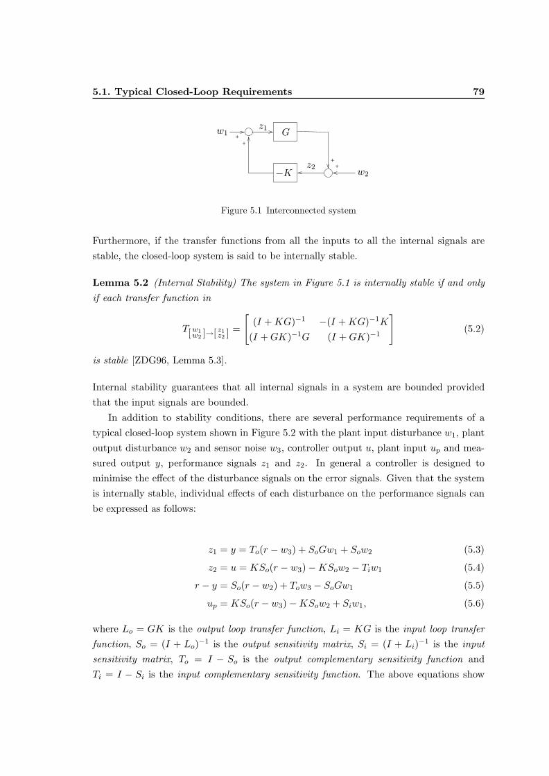
5.1. Typical Closed-Loop Requirements 79
+
+
+
+
z2w2
z1w1
−K
G
Figure 5.1 Interconnected system
Furthermore, if the transfer functions from all the inputs to all the internal signals arestable, the closed-loop system is said to be internally stable.
Lemma 5.2 (Internal Stability) The system in Figure 5.1 is internally stable if and onlyif each transfer function in
T[w1w2 ]→[ z1z2 ] =
[(I +KG)−1 −(I +KG)−1K
(I +GK)−1G (I +GK)−1
](5.2)
is stable [ZDG96, Lemma 5.3].
Internal stability guarantees that all internal signals in a system are bounded providedthat the input signals are bounded.
In addition to stability conditions, there are several performance requirements of atypical closed-loop system shown in Figure 5.2 with the plant input disturbance w1, plantoutput disturbance w2 and sensor noise w3, controller output u, plant input up and mea-sured output y, performance signals z1 and z2. In general a controller is designed tominimise the effect of the disturbance signals on the error signals. Given that the systemis internally stable, individual effects of each disturbance on the performance signals canbe expressed as follows:
z1 = y = To(r − w3) + SoGw1 + Sow2 (5.3)
z2 = u = KSo(r − w3)−KSow2 − Tiw1 (5.4)
r − y = So(r − w2) + Tow3 − SoGw1 (5.5)
up = KSo(r − w3)−KSow2 + Siw1, (5.6)
where Lo = GK is the output loop transfer function, Li = KG is the input loop transferfunction, So = (I + Lo)−1 is the output sensitivity matrix, Si = (I + Li)−1 is the inputsensitivity matrix, To = I − So is the output complementary sensitivity function andTi = I − Si is the input complementary sensitivity function. The above equations show

80 Robust Control System Design
−r
u
z1z2 w1
up
w2
y
w3
K G
Figure 5.2 Standard feedback configuration
the fundamental relationships between the input and output signals in a feedback systemand reveal some important insights for the controller design such as:
σ(So)� 1, for w2 rejection at y
σ(SoG) = σ(GSi)� 1, for w1 rejection at y
σ(Si)� 1, for w1 rejection at up
σ(SiK) = σ(KSo)� 1, for w2 rejection at up.
Furthermore, it can be shown that for rejecting w2 at y, and w1 at up following implicationshold,
σ(So)� 1⇐⇒σ(GK)� 1,
σ(Si)� 1⇐⇒σ(KG)� 1.
Finally, the following approximations hold, when σ(GK)� 1 or σ(KG)� 1, and G andK are square and invertible:
• σ(SoG) ≈ 1σ(K) . Hence, for disturbance rejection at y the output loop gain, σ(GK),
should be large in the frequency range where w2 is significant and the singular valuesof the controller K and σ(GK) should be large in the frequency range where w1 issignificant.
• σ(KSo) ≈ 1σ(G) . Good performance at plant input up requires large input loop gain,
σ(KG), in the frequency range where w1 is significant, and large plant singularvalues and large σ(GK) in the frequency range where w2 is significant. However, wecannot affect the singular values of the plant, thus they impose a limitation on thedesign.
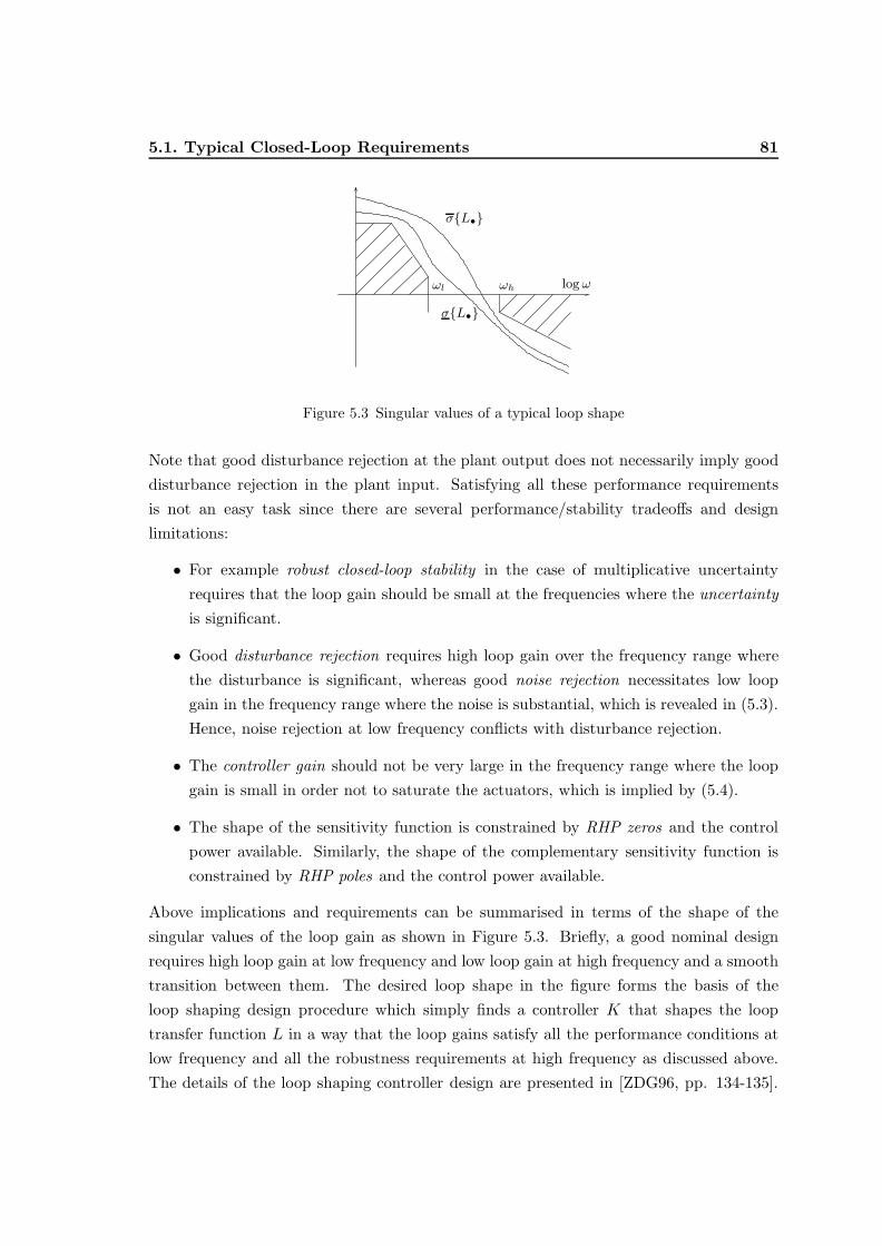
5.1. Typical Closed-Loop Requirements 81
σ{L•}
σ{L•}
log ωωhωl
Figure 5.3 Singular values of a typical loop shape
Note that good disturbance rejection at the plant output does not necessarily imply gooddisturbance rejection in the plant input. Satisfying all these performance requirementsis not an easy task since there are several performance/stability tradeoffs and designlimitations:
• For example robust closed-loop stability in the case of multiplicative uncertaintyrequires that the loop gain should be small at the frequencies where the uncertaintyis significant.
• Good disturbance rejection requires high loop gain over the frequency range wherethe disturbance is significant, whereas good noise rejection necessitates low loopgain in the frequency range where the noise is substantial, which is revealed in (5.3).Hence, noise rejection at low frequency conflicts with disturbance rejection.
• The controller gain should not be very large in the frequency range where the loopgain is small in order not to saturate the actuators, which is implied by (5.4).
• The shape of the sensitivity function is constrained by RHP zeros and the controlpower available. Similarly, the shape of the complementary sensitivity function isconstrained by RHP poles and the control power available.
Above implications and requirements can be summarised in terms of the shape of thesingular values of the loop gain as shown in Figure 5.3. Briefly, a good nominal designrequires high loop gain at low frequency and low loop gain at high frequency and a smoothtransition between them. The desired loop shape in the figure forms the basis of theloop shaping design procedure which simply finds a controller K that shapes the looptransfer function L in a way that the loop gains satisfy all the performance conditions atlow frequency and all the robustness requirements at high frequency as discussed above.The details of the loop shaping controller design are presented in [ZDG96, pp. 134-135].

82 Robust Control System Design
Unfortunately, the designer must shape not only the magnitude but also the phase ofthe loop for achieving stability and performance requirements in the classical loop shaping(but not in the H∞ loop shaping). This makes the classical loop shaping design procedurearduous to apply for difficult systems such as non-minimum phase plants, unstable plantsor MIMO systems.
5.2 H∞ Control with Linear Matrix Inequalities
A linear matrix inequality is a matrix inequality of the form
F (x) := F0 +m∑i=1
xiFi > 0 (or ≥ 0),
where x := [x1 x2 · · · xm]′ ∈ Rm is the vector of decision variables and the matricesFi = F ′i are given. Thus LMIs as given above are convex constraints on the variablex. Multiple LMIs F 1(x) > 0, · · · , F p(x) > 0 may be combined into a single LMI to givediag[F 1(x), · · · , F p(x)] > 0. A wide variety of problems in systems and control theorycan be written as optimisation problems with LMI constraints such as the matrix scalingsproblems or multi-objective control problems [PZPB91, BBFE93, SGC97, AT00]. An his-torical account of the LMIs in control is presented in [BF94]. Analytic solutions to theseLMIs generally do not exist, but efficient numerical methods are available to find a feasiblesolution [GNLC95]. Some nonlinear convex inequalities can be converted into LMI formusing Schur Complements. The following lemma states such an equivalence.
Lemma 5.3 (Schur Complement) Suppose that P = P ′ ∈ Cn×n, R = R′ ∈ Cm×m andS ∈ Cn×m. Then
R < 0 and P − SR−1S′ < 0 ⇔[P S
S′ R
]< 0.
[GA94, Lemma 3.2]
The generic framework for synthesis of optimal H∞ control problems is depicted inFigure 5.4. The standard closed-loop system as given in Figure 5.2 can be always put intothis generic framework.
The plant P represents the generalised plant and takes the following state space form, x
z
y
=
A Bw Bu
Cz Dzw Dzu
Cy Dyw 0
x
w
u
(5.7)

5.2. H∞ Control with Linear Matrix Inequalities 83
u
z1
zn
w1
wn
y
K
P
Figure 5.4 LFT control system synthesis framework
where w = [w1 · · ·wm]′ and z = [z1 · · · zm]′. In this framework the controller K is designedto achieve some bound on the closed-loop transfer function T = Fl (P,K) in some measure.Various measures are available for bounding T such as H2 and H∞ norms. The H2
performance bound is useful to handle stochastic aspects such as the measurement noiseand random disturbances. On the other hand the H∞ performance bound, which isused for the robust controller analysis and synthesis, is convenient to enforce robustnessto model uncertainty and to express frequency-domain specifications such as bandwidth,low-frequency gain, and roll-off. For a more complete discussion of various measures forperformance specifications refer to [SGC97].
The analysis results are presented for the closed-loop system T with the following statespace form,
z = Tw
=
[A BC D
]w. (5.8)
Definition 5.1 (Quadratic Performance) The system (5.8) is said to have quadratic per-formance with respect to the performance index
Pp =
(Qp Sp
S′p Rp
), and Rp ≥ 0 (5.9)
if it is asymptotically stable and if there exists an β > 0 such that:
∫ ∞0
(w(t)z(t)
)′Pp
(w(t)z(t)
)dt ≤ −β ‖w‖2 , for every w ∈ L2 (5.10)
[Sch00, Section 3.2].
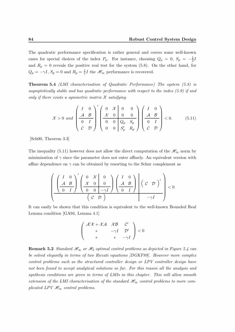
84 Robust Control System Design
The quadratic performance specification is rather general and covers some well-knowncases for special choices of the index Pp. For instance, choosing Qp = 0, Sp = −1
2I
and Rp = 0 reveals the positive real test for the system (5.8). On the other hand, forQp = −γI, Sp = 0 and Rp = 1
γ I the H∞ performance is recovered.
Theorem 5.4 (LMI characterisation of Quadratic Performance) The system (5.8) isasymptotically stable and has quadratic performance with respect to the index (5.9) if andonly if there exists a symmetric matrix X satisfying
X > 0 and
I 0A B0 I
C D
′
0 X 0 0X 0 0 0
0 0 Qp Sp
0 0 S′p Rp
I 0A B0 I
C D
< 0. (5.11)
[Sch00, Theorem 3.3]
The inequality (5.11) however does not allow the direct computation of the H∞ norm byminimisation of γ since the parameter does not enter affinely. An equivalent version withaffine dependence on γ can be obtained by resorting to the Schur complement as
I 0A B0 I
′ 0 X 0X 0 0
0 0 −γI
I 0A B0 I
(C D
)′(C D
)−γI
< 0
It can easily be shown that this condition is equivalent to the well-known Bounded RealLemma condition [GA94, Lemma 4.1] A
′X + XA XB C′
∗ −γI D′
∗ ∗ −γI
< 0
Remark 5.2 Standard H∞ or H2 optimal control problems as depicted in Figure 5.4 canbe solved elegantly in terms of two Riccati equations [DGKF89]. However more complexcontrol problems such as the structured controller design or LPV controller design havenot been found to accept analytical solutions so far. For this reason all the analysis andsynthesis conditions are given in terms of LMIs in this chapter. This will allow smoothextension of the LMI characterisation of the standard H∞ control problems to more com-plicated LPV H∞ control problems.
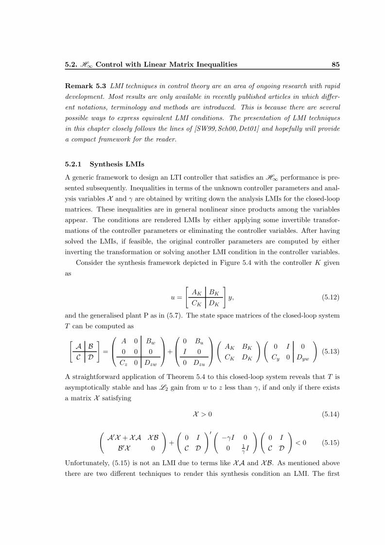
5.2. H∞ Control with Linear Matrix Inequalities 85
Remark 5.3 LMI techniques in control theory are an area of ongoing research with rapiddevelopment. Most results are only available in recently published articles in which differ-ent notations, terminology and methods are introduced. This is because there are severalpossible ways to express equivalent LMI conditions. The presentation of LMI techniquesin this chapter closely follows the lines of [SW99,Sch00,Det01] and hopefully will providea compact framework for the reader.
5.2.1 Synthesis LMIs
A generic framework to design an LTI controller that satisfies an H∞ performance is pre-sented subsequently. Inequalities in terms of the unknown controller parameters and anal-ysis variables X and γ are obtained by writing down the analysis LMIs for the closed-loopmatrices. These inequalities are in general nonlinear since products among the variablesappear. The conditions are rendered LMIs by either applying some invertible transfor-mations of the controller parameters or eliminating the controller variables. After havingsolved the LMIs, if feasible, the original controller parameters are computed by eitherinverting the transformation or solving another LMI condition in the controller variables.
Consider the synthesis framework depicted in Figure 5.4 with the controller K givenas
u =
[AK BK
CK DK
]y, (5.12)
and the generalised plant P as in (5.7). The state space matrices of the closed-loop systemT can be computed as
[A BC D
]=
A 0 Bw
0 0 0
Cz 0 Dzw
+
0 Bu
I 0
0 Dzu
( AK BK
CK DK
)(0 I 0Cy 0 Dyw
)(5.13)
A straightforward application of Theorem 5.4 to this closed-loop system reveals that T isasymptotically stable and has L2 gain from w to z less than γ, if and only if there existsa matrix X satisfying
X > 0 (5.14)
(A′X + XA XBB′X 0
)+
(0 I
C D
)′(−γI 0
0 1γ I
)(0 I
C D
)< 0 (5.15)
Unfortunately, (5.15) is not an LMI due to terms like XA and XB. As mentioned abovethere are two different techniques to render this synthesis condition an LMI. The first

86 Robust Control System Design
technique, also first historically, uses the elimination lemma [GA94, Lemma 3.1] to re-cover the convexity. We will call this method “synthesis via elimination of variables”hereafter. The second technique uses some congruence transformations to obtain LMIs insome transformed controller variables [CG96,SGC97]. We will call this method “synthesisvia change of variables” hereafter. In the following both techniques are presented for H∞
controller design. The synthesis via change of variables method is presented first.
Controller Synthesis via Change of Variables
As a first step towards rendering the problem convex , partition X and X−1 as,
X =
(X U
U ′ •
), X−1 =
(Y V
V ′ •
), (5.16)
where X, Y , U , V have same dimensions as A and • indicates entries that are not relevantfor what follows. Consider
Y =
(Y I
V ′ 0
)(5.17)
with
Y ′X =
(Y V
I 0
)(X U
U ′ •
)=
(I 0X U
)(5.18)
Using Y and
(Y 00 I
)to perform a congruence transformation on (5.14) and on (5.15)
respectively, the following theorem is obtained.
Theorem 5.5 (Synthesis via Change of Variables) There exist a controller
(AK BK
CK DK
)and a matrix X which satisfy (5.14) and (5.15) if and only if the following LMIs in X,Y , K, L, M , N admit a feasible solution,(
Y I
I X
)> 0 (5.19)
(
A′ + A B
B′ 0
)+
(0 I
C D
)′(−γI 0
0 0
)(0 I
C D
) (C D
)′T ′p
Tp
(C D
)−I
< 0
(5.20)where 1
γ I = T ′pTp and
(A B
C D
)=
AY +BuM A+BuNCy Bw +BuNDyw
K XA+ LCy XBw + LDyw
CzY +DzuM Cz +DzuNCy Dzw +DzuNDyw
(5.21)

5.2. H∞ Control with Linear Matrix Inequalities 87
If a feasible solution exists, a controller and a matrix X that solve (5.14) and (5.15) canbe computed as
i. Compute two full-column rank matrices U and V such that I −XY = UV ′.
ii. Construct controller matrices as(AK BK
CK DK
)=
(U XB
0 I
)−1(K −XAY L
M N
)(V ′ 0CY I
)−1
. (5.22)
iii. Determine the Lyapunov matrix X as
X =
(Y V
I 0
)−1(I 0X U
)(5.23)
[Det01, Theorem 18]
Matrix inequality (5.20) does not allow direct minimisation of the L2 gain, since γ doesnot appear in an affine manner. An equivalent LMI condition, which is more user friendly,can be obtained through elementary matrix operations and Schur complement argumentsas [SGC97]
XA+ (∗) + LCy + (∗) ∗ ∗ ∗K ′ +A+BuNCy AY + (∗) +BuM + (∗) ∗ ∗(XBw + LDyw)′ (Bw +BuNDyw)′ −γI ∗Cz +DzuNCy CzY +DzuM Dzw +DzuNDyw −γI
< 0
(5.24)The parameter transformation (5.21) plays a crucial role in several difficult synthesis prob-lems such as the H∞ control with pole placement constraints [CG96] or multi-objectiveoutput feedback control [SGC97].
Controller Synthesis via Elimination of Variables
The synthesis procedure via variable elimination is not as general as the synthesis viatransformation of variables since the possibility of eliminating variables depends on thenumber and on the structure of the underlying LMIs. In problems in which the controllerparameters appear in one LMI only it is possible to eliminate all the controller parameters.In the following controller synthesis by elimination of variables for the H∞ performanceis described.

88 Robust Control System Design
Theorem 5.6 (Synthesis via Elimination of Variables) There exists a stabilising con-troller that achieves ‖T‖∞ < γ0 if and only if there exists X and Y that solve the followinginequalities for γ = γ0, (
Y I
I X
)> 0 (5.25)
(φ1
φ2
)′I 00 I
XA XBw
Cz Dzw
′
0 0 I 00 −γI 0 0
I 0 0 00 0 0 1
γ I
I 00 I
XA XBw
Cz Dzw
(φ1
φ2
)< 0 (5.26)
(ψ1
ψ2
)′−Y A′ −Y C ′z−B′w −D′zwI 00 I
′
0 0 I 00 − 1
γ I 0 0
I 0 0 00 0 0 γI
−Y A′ −Y C ′z−B′w −D′zwI 00 I
(ψ1
ψ2
)> 0
(5.27)
where
(φ1
φ2
)and
(ψ1
ψ2
)denote bases of the null spaces of (Cy,Dyw) and (B′u,D
′zu)
respectively [Det01, Theorem 22].
In the present form the inequalities in Theorem 5.6 do not allow a direct minimisation ofγ in order to determine the optimal H∞ performance, since they do not depend affinelyon this parameter. As usual, equivalent LMI conditions can be obtained via Schur com-plement arguments. In fact inequalities (5.26) and (5.27) can be rewritten in their morefamiliar form as [GA94]
(φ 0
0 I
)′ XA+A′X XBw C ′z∗ −γI D′zw∗ ∗ −γI
( φ 0
0 I
)< 0 (5.28)
(ψ 0
0 I
)′ Y A′ +AY Y C ′z Bw
∗ −γI Dzw
∗ ∗ −γI
( ψ 0
0 I
)< 0 (5.29)
with φ =
(φ1
φ2
)and ψ =
(ψ1
ψ2
).
Theorem 5.6 guarantees only the existence of a γ-suboptimal H∞ controller, but itdoes not directly offer a way to compute it. There are several ways of computing the

5.2. H∞ Control with Linear Matrix Inequalities 89
controller after having solved the above LMIs for X, Y and γ. One way is to compute Xvia the factorisation I−XY = UV ′ and (5.23). Once X has been calculated, the controllerparameters AK , BK , CK , DK can be obtained by directly solving (5.15). Another way isto use the explicit controller formulae given in [IS94,Gah96]
Remark 5.4 The synthesis via elimination of variables requires the solution of two se-quential systems of LMIs: one for computing X and Y , and one for computing the con-troller parameters. On the other hand the synthesis via transformation of variables requiresthe solution of only one system of LMIs, but with a larger number of decision variables.This makes the synthesis via elimination of variables the only method to obtain numericallytractable solutions for problems of large size.
5.2.2 Example: LTI H∞ Loop Shaping Controller Design
This example will demonstrate some features of the robust control system design in theH∞ loop shaping paradigm which is described briefly in Appendix C for completenessand convenience of the reader. The plant considered is a simplified AFR path model withtwo sub-blocks. The LTI part of the model, denoted Gx, is the identified gas mixing andsensor dynamics at Pm = 40kPa, IVO=−5◦, EVC=10◦ ATDC,
Gx(z) =0.06273
z2 − 1.516z + 0.5792(5.30)
The time-varying part is an output delay that varies from 8 events at 30kPa to 2 eventsat 60kPa linearly. A second order approximation in LFT form is used to approximate thedelay as suggested in Section 4.3. The overall plant G can be expressed as an upper LFTof the normalised manifold pressure ρ in the event based discrete-time as G = Fu (P,∆),where
P =
0 1 0 0 0 0 0−0.5792 1.5165 0 0 0 0 0.0627280.57143 0 0.42857 0 0.85714 0 0−0.2449 0 0.81633 0.42857 0.4898 0.85714 0
0.28571 0 −0.28571 0 0.42857 0 0−0.12245 0 0.40816 −0.28571 0.2449 0.42857 00.18367 0 −0.61224 1.4286 −0.36735 0.85714 0
(5.31)
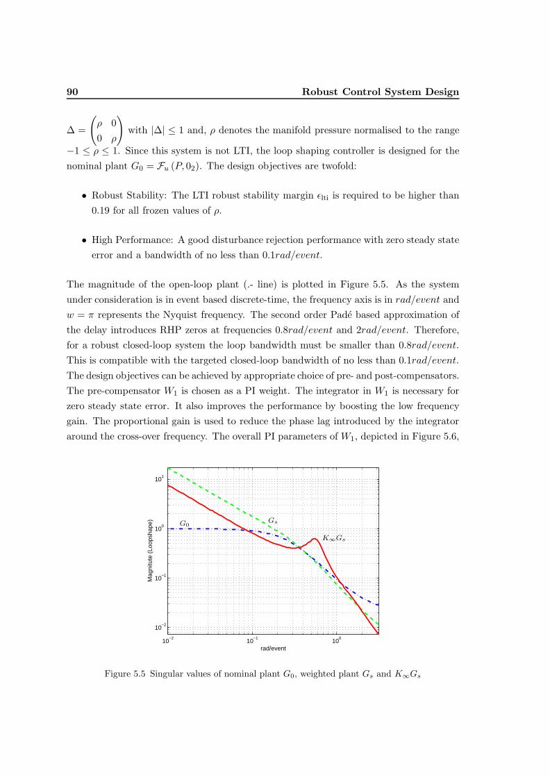
90 Robust Control System Design
∆ =
(ρ 00 ρ
)with |∆| ≤ 1 and, ρ denotes the manifold pressure normalised to the range
−1 ≤ ρ ≤ 1. Since this system is not LTI, the loop shaping controller is designed for thenominal plant G0 = Fu (P, 02). The design objectives are twofold:
• Robust Stability: The LTI robust stability margin εlti is required to be higher than0.19 for all frozen values of ρ.
• High Performance: A good disturbance rejection performance with zero steady stateerror and a bandwidth of no less than 0.1rad/event.
The magnitude of the open-loop plant (.- line) is plotted in Figure 5.5. As the systemunder consideration is in event based discrete-time, the frequency axis is in rad/event andw = π represents the Nyquist frequency. The second order Pade based approximation ofthe delay introduces RHP zeros at frequencies 0.8rad/event and 2rad/event. Therefore,for a robust closed-loop system the loop bandwidth must be smaller than 0.8rad/event.This is compatible with the targeted closed-loop bandwidth of no less than 0.1rad/event.The design objectives can be achieved by appropriate choice of pre- and post-compensators.The pre-compensator W1 is chosen as a PI weight. The integrator in W1 is necessary forzero steady state error. It also improves the performance by boosting the low frequencygain. The proportional gain is used to reduce the phase lag introduced by the integratoraround the cross-over frequency. The overall PI parameters of W1, depicted in Figure 5.6,
10−2
10−1
100
10−2
10−1
100
101
rad/event
Mag
nitu
te (
Loop
shap
e) GsG0
K∞Gs
Figure 5.5 Singular values of nominal plant G0, weighted plant Gs and K∞Gs
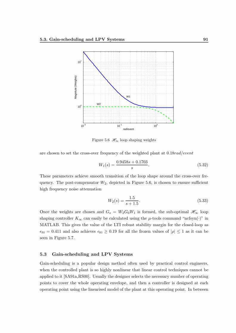
5.3. Gain-scheduling and LPV Systems 91
10−2
10−1
100
100
101
rad/event
Mag
nitu
te (
Wei
ghts
)
W1
W2
Figure 5.6 H∞ loop shaping weights
are chosen to set the cross-over frequency of the weighted plant at 0.18rad/event
W1(s) =0.9458s + 0.1703
s. (5.32)
These parameters achieve smooth transition of the loop shape around the cross-over fre-quency. The post-compensator W2, depicted in Figure 5.6, is chosen to ensure sufficienthigh frequency noise attenuation
W2(s) =1.5
s+ 1.5. (5.33)
Once the weights are chosen and Gs = W2G0W1 is formed, the sub-optimal H∞ loopshaping controller K∞ can easily be calculated using the µ-tools command “ncfsyn(·)” inMATLAB. This gives the value of the LTI robust stability margin for the closed-loop asεlti = 0.411 and also achieves εlti ≥ 0.19 for all the frozen values of |ρ| ≤ 1 as it can beseen in Figure 5.7.
5.3 Gain-scheduling and LPV Systems
Gain-scheduling is a popular design method often used by practical control engineers,when the controlled plant is so highly nonlinear that linear control techniques cannot beapplied to it [SA91a,RS00]. Usually the designer selects the necessary number of operatingpoints to cover the whole operating envelope, and then a controller is designed at eachoperating point using the linearised model of the plant at this operating point. In between

92 Robust Control System Design
−1 −0.8 −0.6 −0.4 −0.2 0 0.2 0.4 0.6 0.8 10.15
0.2
0.25
0.3
0.35
0.4
0.45
0.5
ρ
Robust
Sta
bil
ity
Marg
inεlt
i
Figure 5.7 Robust Stability margin for the frozen values of ρ
the operating points, the parameters (gains) of the controllers are interpolated to cover thewhole operating envelope. The result is a global feedback law obtained by gain-scheduling.The main drawback is the lack of guarantees that show that the interpolation of the LTIcontrollers will stabilise the nonlinear plant. This is because the global feedback lawresulted from the gain-scheduling is a nonlinear controller and the guarantees of the linearsynthesis methods do not hold anymore even though the gain scheduled controllers areknown to work in practise. Hence, the designer spends most of his/her time to show thatthe gain-scheduling controller performs well by extensive computer simulations, as onecannot assess a priori the guaranteed stability, robustness, and performance propertiesof the gain-scheduled control law. Two prominent gain-scheduling guidelines are [SA90,SA91b]
• The scheduling variables should capture the plant’s nonlinearities;
• The scheduling variables should vary slowly;
These guidelines also reveal the fundamental limitations on the achievable performanceby the gain-scheduling design.
In contrast to the classical gain-scheduling techniques discussed above, the recentlydeveloped robust gain-scheduling methods [RS00] in the LPV framework provide system-atic ways to design controllers that are scheduled on the operating point of the system.An LPV system is a linear system whose describing matrices depend on a time-varying
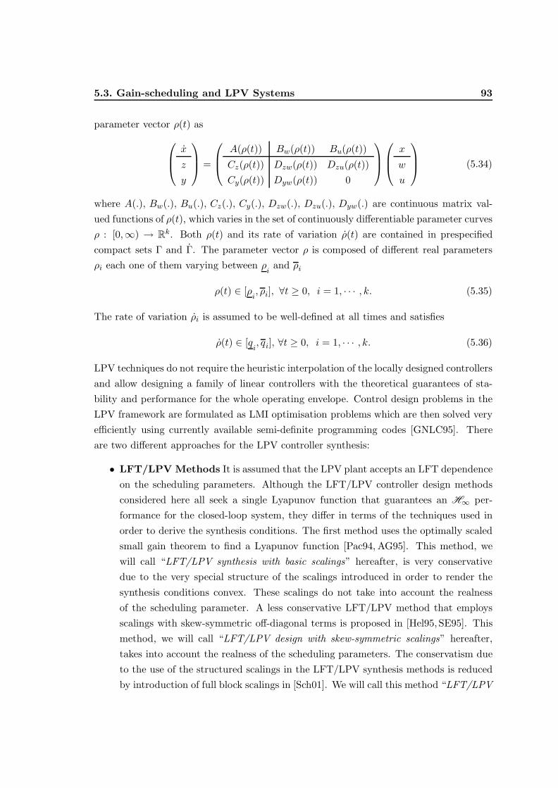
5.3. Gain-scheduling and LPV Systems 93
parameter vector ρ(t) as x
z
y
=
A(ρ(t)) Bw(ρ(t)) Bu(ρ(t))
Cz(ρ(t)) Dzw(ρ(t)) Dzu(ρ(t))Cy(ρ(t)) Dyw(ρ(t)) 0
x
w
u
(5.34)
where A(.), Bw(.), Bu(.), Cz(.), Cy(.), Dzw(.), Dzu(.), Dyw(.) are continuous matrix val-ued functions of ρ(t), which varies in the set of continuously differentiable parameter curvesρ : [0,∞) → Rk. Both ρ(t) and its rate of variation ρ(t) are contained in prespecifiedcompact sets Γ and Γ. The parameter vector ρ is composed of different real parametersρi each one of them varying between ρ
iand ρi
ρ(t) ∈ [ρi, ρi], ∀t ≥ 0, i = 1, · · · , k. (5.35)
The rate of variation ρi is assumed to be well-defined at all times and satisfies
ρ(t) ∈ [qi, qi], ∀t ≥ 0, i = 1, · · · , k. (5.36)
LPV techniques do not require the heuristic interpolation of the locally designed controllersand allow designing a family of linear controllers with the theoretical guarantees of sta-bility and performance for the whole operating envelope. Control design problems in theLPV framework are formulated as LMI optimisation problems which are then solved veryefficiently using currently available semi-definite programming codes [GNLC95]. Thereare two different approaches for the LPV controller synthesis:
• LFT/LPV Methods It is assumed that the LPV plant accepts an LFT dependenceon the scheduling parameters. Although the LFT/LPV controller design methodsconsidered here all seek a single Lyapunov function that guarantees an H∞ per-formance for the closed-loop system, they differ in terms of the techniques used inorder to derive the synthesis conditions. The first method uses the optimally scaledsmall gain theorem to find a Lyapunov function [Pac94, AG95]. This method, wewill call “LFT/LPV synthesis with basic scalings” hereafter, is very conservativedue to the very special structure of the scalings introduced in order to render thesynthesis conditions convex. These scalings do not take into account the realnessof the scheduling parameter. A less conservative LFT/LPV method that employsscalings with skew-symmetric off-diagonal terms is proposed in [Hel95, SE95]. Thismethod, we will call “LFT/LPV design with skew-symmetric scalings” hereafter,takes into account the realness of the scheduling parameters. The conservatism dueto the use of the structured scalings in the LFT/LPV synthesis methods is reducedby introduction of full block scalings in [Sch01]. We will call this method “LFT/LPV
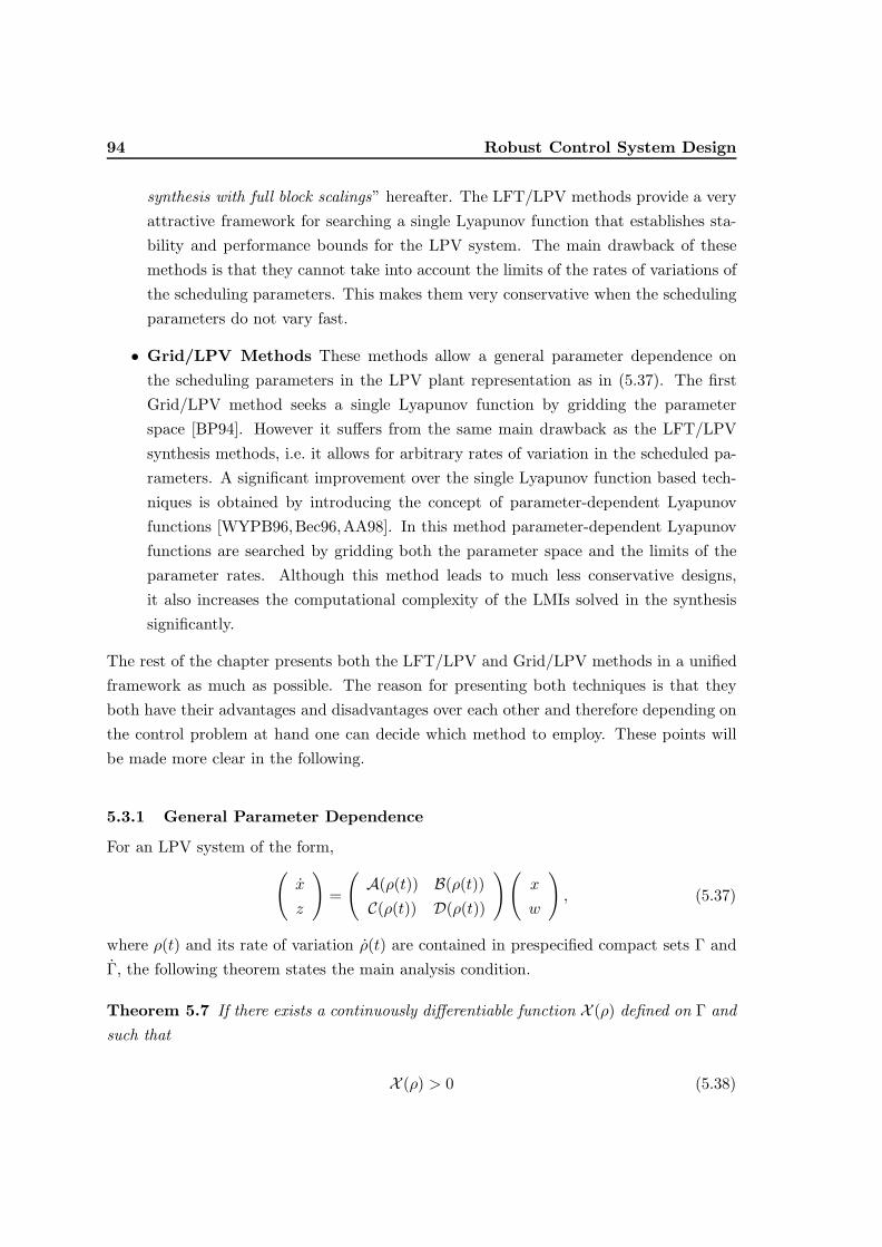
94 Robust Control System Design
synthesis with full block scalings” hereafter. The LFT/LPV methods provide a veryattractive framework for searching a single Lyapunov function that establishes sta-bility and performance bounds for the LPV system. The main drawback of thesemethods is that they cannot take into account the limits of the rates of variations ofthe scheduling parameters. This makes them very conservative when the schedulingparameters do not vary fast.
• Grid/LPV Methods These methods allow a general parameter dependence onthe scheduling parameters in the LPV plant representation as in (5.37). The firstGrid/LPV method seeks a single Lyapunov function by gridding the parameterspace [BP94]. However it suffers from the same main drawback as the LFT/LPVsynthesis methods, i.e. it allows for arbitrary rates of variation in the scheduled pa-rameters. A significant improvement over the single Lyapunov function based tech-niques is obtained by introducing the concept of parameter-dependent Lyapunovfunctions [WYPB96,Bec96,AA98]. In this method parameter-dependent Lyapunovfunctions are searched by gridding both the parameter space and the limits of theparameter rates. Although this method leads to much less conservative designs,it also increases the computational complexity of the LMIs solved in the synthesissignificantly.
The rest of the chapter presents both the LFT/LPV and Grid/LPV methods in a unifiedframework as much as possible. The reason for presenting both techniques is that theyboth have their advantages and disadvantages over each other and therefore depending onthe control problem at hand one can decide which method to employ. These points willbe made more clear in the following.
5.3.1 General Parameter Dependence
For an LPV system of the form,(x
z
)=
(A(ρ(t)) B(ρ(t))C(ρ(t)) D(ρ(t))
)(x
w
), (5.37)
where ρ(t) and its rate of variation ρ(t) are contained in prespecified compact sets Γ andΓ, the following theorem states the main analysis condition.
Theorem 5.7 If there exists a continuously differentiable function X (ρ) defined on Γ andsuch that
X (ρ) > 0 (5.38)
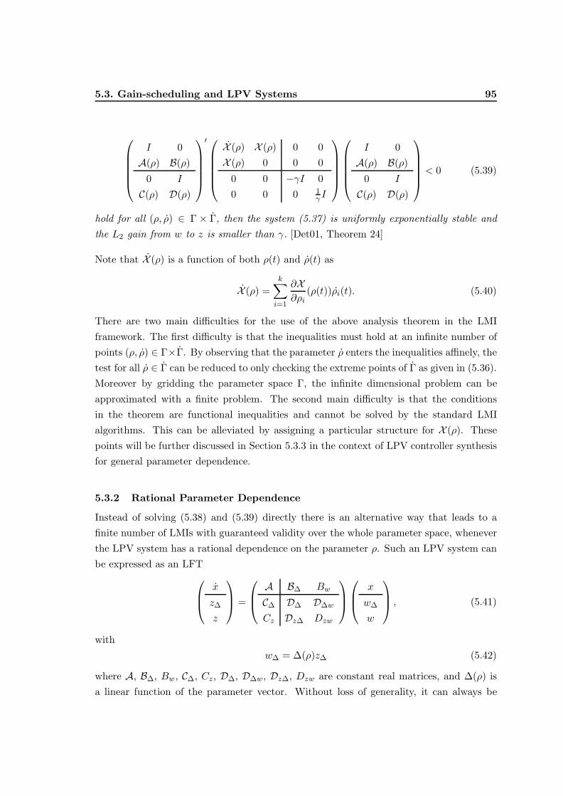
5.3. Gain-scheduling and LPV Systems 95
I 0A(ρ) B(ρ)
0 I
C(ρ) D(ρ)
′X (ρ) X (ρ) 0 0X (ρ) 0 0 0
0 0 −γI 00 0 0 1
γ I
I 0A(ρ) B(ρ)
0 I
C(ρ) D(ρ)
< 0 (5.39)
hold for all (ρ, ρ) ∈ Γ × Γ, then the system (5.37) is uniformly exponentially stable andthe L2 gain from w to z is smaller than γ. [Det01, Theorem 24]
Note that X (ρ) is a function of both ρ(t) and ρ(t) as
X (ρ) =k∑i=1
∂X∂ρi
(ρ(t))ρi(t). (5.40)
There are two main difficulties for the use of the above analysis theorem in the LMIframework. The first difficulty is that the inequalities must hold at an infinite number ofpoints (ρ, ρ) ∈ Γ×Γ. By observing that the parameter ρ enters the inequalities affinely, thetest for all ρ ∈ Γ can be reduced to only checking the extreme points of Γ as given in (5.36).Moreover by gridding the parameter space Γ, the infinite dimensional problem can beapproximated with a finite problem. The second main difficulty is that the conditionsin the theorem are functional inequalities and cannot be solved by the standard LMIalgorithms. This can be alleviated by assigning a particular structure for X (ρ). Thesepoints will be further discussed in Section 5.3.3 in the context of LPV controller synthesisfor general parameter dependence.
5.3.2 Rational Parameter Dependence
Instead of solving (5.38) and (5.39) directly there is an alternative way that leads to afinite number of LMIs with guaranteed validity over the whole parameter space, wheneverthe LPV system has a rational dependence on the parameter ρ. Such an LPV system canbe expressed as an LFT x
z∆
z
=
A B∆ Bw
C∆ D∆ D∆w
Cz Dz∆ Dzw
x
w∆
w
, (5.41)
withw∆ = ∆(ρ)z∆ (5.42)
where A, B∆, Bw, C∆, Cz, D∆, D∆w, Dz∆, Dzw are constant real matrices, and ∆(ρ) isa linear function of the parameter vector. Without loss of generality, it can always be

96 Robust Control System Design
chosen as ∆(ρ) = diag(ρ1I1, ..., ρkIk). A straightforward application of the full block S-procedure [Sch01] to (5.39) with the LPV system given by the LFT representation (5.41)leads to the following analysis characterisation for the LFT/LPV synthesis methods.
Theorem 5.8 If there exists a symmetric matrix X and scalings Q = Q′, S, and R = R′
such thatX > 0 (5.43)
and
I 0 0A Bw B∆
0 I 0Cz Dzw Dz∆0 0 I
C∆ D∆w D∆
′
0 X 0 0 0 0X 0 0 0 0 0
0 0 −γI 0 0 00 0 0 1
γ I 0 0
0 0 0 0 Q S
0 0 0 0 S′ R
I 0 0A Bw B∆
0 I 0Cz Dzw Dz∆0 0 I
C∆ D∆w D∆
< 0 (5.44)
and (∆(ρ)I
)′(Q S
S′ R
)(∆(ρ)I
)> 0 for all ρ ∈ Γ (5.45)
then the system in (5.41) is uniformly exponentially stable and L2 gain from w to z issmaller than γ for all ρ(t) which is continuously differentiable and satisfies ρ(t) ∈ Γ forall t [Det01, Theorem 26].
Note that the above theorem does not put any bounds on ρ and allows arbitrarly fastvariations in the parameter vector ρ. Computationally tractable conditions for (5.45)are obtained through the choice of suitable sets of scalings. This will be discussed in Sec-tion 5.3.4 when the LMI synthesis conditions for the LFT/LPV methods will be presented.
Next we will show that L2 gain is preserved under the Tustin’s transformation for anLFT/LPV system. Consider the matrix inequality (5.44), which can be rewritten as
I 0 0A Bw B∆
0 I 00 0 I
Cz Dzw Dz∆C∆ D∆w D∆
′
︸ ︷︷ ︸
I 0A B
0 I
C D
′
0 X 0 0 0 0X 0 0 0 0 0
0 0 −γI 0 0 00 0 0 Q 0 S
0 0 0 0 1γ I 0
0 0 0 S′ 0 R
︸ ︷︷ ︸
0 X 0 0X 0 0 0
0 0 Q S
0 0 S′ R
I 0 0A Bw B∆
0 I 00 0 I
Cz Dzw Dz∆C∆ D∆w D∆
︸ ︷︷ ︸
I 0A B
0 I
C D
< 0 (5.46)

5.3. Gain-scheduling and LPV Systems 97
Matrix inequalities (5.43), (5.46) represent the L2 γ-gain condition for a continuous-timeLFT system described by (A,B,C,D). If the state space data (A,B,C,D) are actuallyobtained from a discrete-time state space data (A, B, C, D, Ts) via Tustin’s transformation,i.e. [
A B
C D
]=
[2Ts
(A+ I)−1(A− I) 2√Ts
(A+ I)−1B2√TsC(A+ I)−1 D − C(A+ I)−1B
], (5.47)
then, it can be shown after some simple matrix algebra that applying the following simi-larity and congruence transformations, M and L, on (5.46) as suggested below
(M 0
0 I
)I 0A B
0 I
C D
L =
I 0A B
0 I
C D
, (5.48)
(M 0
0 I
)′−1
0 X 0 0X 0 0 0
0 0 Q S
0 0 S′ R
(M 0
0 I
)−1
=
−X 0 0 0
0 X 0 0
0 0 Q S
0 0 S′ R
, (5.49)
with
L =
[√Ts2 (A+ I)
√Ts2 B
0 I
](5.50)
M =
[I√Ts−√Ts2 I
I√Ts
√Ts2 I
](5.51)
transforms (5.46) to the equivalent L2 γ-gain condition for the discrete-time system(A, B, C, D, Ts) as
X > 0, (5.52)I 0A B
0 I
C D
′−X 0 0 0
0 X 0 0
0 0 Q S
0 0 S′ R
I 0A B
0 I
C D
< 0 (5.53)
where X = X , Q = Q, S = S, R = R. This concludes that analysing the L2 gain of adiscrete-time LFT/LPV system (A, B, C, D, Ts) is equivalent to first taking the Tustin’stransform of the discrete-time system and then applying Theorem 5.8 on the transformedsystem state space data (A,B,C,D).

98 Robust Control System Design
5.3.3 LPV Controller Synthesis for General Parameter Dependence
Consider the generalised LPV plant described in (5.34) with the state space realisation x
z
y
=
A(ρ(t)) Bw(ρ(t)) Bu(ρ(t))
Cz(ρ(t)) Dzw(ρ(t)) Dzu(ρ(t))Cy(ρ(t)) Dyw(ρ(t)) 0
x
w
u
(5.54)
The analysis theorem 5.7 can be applied to the closed-loop LPV system to synthesise acontroller of the form,(
xK
u
)=
(AK(ρ(t), ρ(t)) BK(ρ(t), ρ(t))CK(ρ(t), ρ(t)) DK(ρ(t), ρ(t))
)(xK
y
), (5.55)
to ensure the internal stability and a guaranteed L2 gain bound γ from the disturbancesignal w to the error signal z. The derivation of the LMI conditions for the LPV controllersynthesis follows similar lines as in the case of the LTI controller synthesis in Section 5.2.1.Both the change of variables and elimination of variables techniques can be used to derivethe LPV synthesis conditions. The synthesis via change of variables method is presentedfirst. The dependence of the plant and controller parameters on ρ and ρ has been droppedfor simplicity.
Theorem 5.9 (Synthesis via Change of Variables) Consider the LPV plant governedby (5.54), with the parameter trajectories constrained by (5.35) ,(5.36). There exist a con-troller (5.55) enforcing internal stability and a bound γ on the L2 gain of the closed-loopsystem (5.54) and (5.55), whenever there exist parameter dependent symmetric matricesY and X, and a parameter-dependent quadruple of state space data (K,L,M,N) such thatfor all (ρ, ρ) ∈ Γ× Γ the following infinite dimensional LMI problem holds(
X I
I Y
)> 0 (5.56)
X +XA+ (∗) + · · ·LCy + (∗)
∗ ∗ ∗
K ′ +A+BuNCy−Y +AY + (∗) + · · ·· · ·BuM + (∗)
∗ ∗
(XBw + LDyw)′ (Bw +BuNDyw)′ −γI ∗
Cz +DzuNCy CzY +DzuMDzw + · · ·· · ·DzuNDyw
−γI
< 0
(5.57)If a solution exists, an LPV controller is readily obtained with the following two-step
scheme
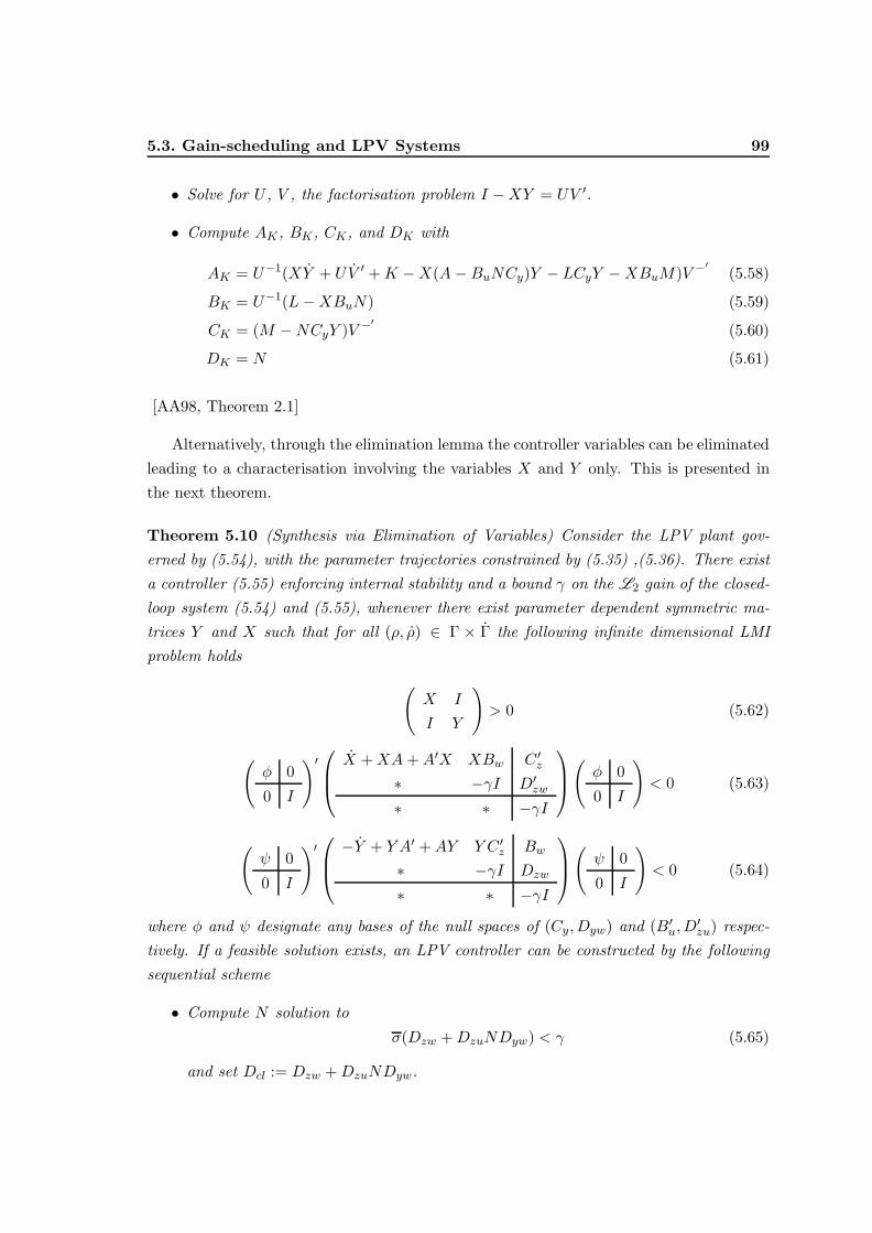
5.3. Gain-scheduling and LPV Systems 99
• Solve for U , V , the factorisation problem I −XY = UV ′.
• Compute AK , BK , CK , and DK with
AK = U−1(XY + UV ′ +K −X(A−BuNCy)Y − LCyY −XBuM)V −′
(5.58)
BK = U−1(L−XBuN) (5.59)
CK = (M −NCyY )V −′
(5.60)
DK = N (5.61)
[AA98, Theorem 2.1]
Alternatively, through the elimination lemma the controller variables can be eliminatedleading to a characterisation involving the variables X and Y only. This is presented inthe next theorem.
Theorem 5.10 (Synthesis via Elimination of Variables) Consider the LPV plant gov-erned by (5.54), with the parameter trajectories constrained by (5.35) ,(5.36). There exista controller (5.55) enforcing internal stability and a bound γ on the L2 gain of the closed-loop system (5.54) and (5.55), whenever there exist parameter dependent symmetric ma-trices Y and X such that for all (ρ, ρ) ∈ Γ × Γ the following infinite dimensional LMIproblem holds (
X I
I Y
)> 0 (5.62)
(φ 0
0 I
)′ X +XA+A′X XBw C ′z∗ −γI D′zw∗ ∗ −γI
( φ 0
0 I
)< 0 (5.63)
(ψ 0
0 I
)′ −Y + Y A′ +AY Y C ′z Bw
∗ −γI Dzw
∗ ∗ −γI
( ψ 0
0 I
)< 0 (5.64)
where φ and ψ designate any bases of the null spaces of (Cy,Dyw) and (B′u,D′zu) respec-
tively. If a feasible solution exists, an LPV controller can be constructed by the followingsequential scheme
• Compute N solution to
σ(Dzw +DzuNDyw) < γ (5.65)
and set Dcl := Dzw +DzuNDyw.

100 Robust Control System Design
• Compute L and M 0 Dyw 0∗ −γI D′cl∗ ∗ −γI
( L′
•
)=
Cy
B′wX
Cz +DzuNCy
(5.66)
0 D′zu 0∗ −γI Dcl
∗ ∗ −γI
( M
•
)=
Bu
CzY
Bw +BuNDyw
(5.67)
• Compute
K = −(A+BuNCy)′ +(XBw + LDyw (Cz +DzuNCy)′
).
(−γI D′cl∗ −γI
)−1((Bw +BuNDyw)′
CzY +DzuM
)(5.68)
• Solve U , V as I −XY = UV ′.
• Compute AK , BK , CK , DK with the help of (5.58)- (5.61).
[AA98, Theorems 2.2 and 2.3]
Note that in spite of their different structures the characterisations given in Theorems 5.9-5.10, are equivalent and can be virtually used interchangeably for controller synthesis.However, in terms of the computational complexity or practical implementation thesetechniques exhibit significant differences. The first method, synthesis via change of vari-ables, allows the incorporation of multiple specifications into the design problem such asmixed H∞-H2 optimisation, pole clustering, or control effort constraints. However, itis computationally very intensive due to a much larger number of decision variables inthe LMI constraints. The second method, synthesis via elimination of variables, althoughmore restrictive, is computationally very attractive due to a much smaller number of de-cision variables. In terms of the practical implementation, controller equations resultingfrom the synthesis via change of variables method are significantly less complex than thoseresulting from the synthesis via elimination of variables method. At each sampling timethe synthesis via change of variables method only requires one matrix inversion, whereasthe synthesis via elimination of variables method requires two QR decompositions, threematrix inversions for (5.65) and two matrix inversions for the computation of AK , BK ,CK , DK . Hence controllers resulting from the first technique are more easily implementedin real-time.
5.3. Gain-scheduling and LPV Systems 101
In the controller implementation, I −XY should be well-conditioned to avoid the ill-conditioned inversions of the matrices U and V . Unfortunately, I − XY will be nearlysingular if the constraint (5.56) or ( 5.62) is saturated at the optimum. This can beprevented by choosing a suboptimal value of γ and including the following LMI(
X tI
tI Y
)> 0 (5.69)
with the additional variable t in the synthesis LMIs and maximising t. This proceduremaximises the minimal eigenvalue of XY and improves the conditioning of I −XY .
The LPV controllers derived from Theorems 5.9-5.10 are not gain-scheduled in theusual sense since they require not only the measurement of the parameters ρ but alsoof their time derivatives ρ. As this is restrictive in many control problems, a simplebut conservative approach is proposed in [Bec96, AA98]. Assuming either X or Y asparameter independent constant matrix variables drop the time derivative dependencein the above theorems. This can be seen by differentiating I −XY = UV ′ and showingXY +UV ′ = XY −UV ′. This equality can be used in (5.58) to show that AK is indepedentof ρ whenever either X = 0 or Y = 0. Due to loss of duality in the variables X and Y ,such choices are not equivalent. Therefore, the usual practice is to try both of the casesand use the less conservative one as the final controller.
The LMI conditions presented above cannot be solved due to two main difficulties.First, the functional dependence of X and Y on ρ has to be decided in order to render theconditions to standard LMIs. A useful guideline is to mimic the parameter dependenceof the plant in the Lyapunov function variables X and Y . In the case of the synthesisvia change of variables method, structures for the parameters K, L, M , N should also beassigned in a similar manner. Second, the synthesis LMIs, which have to be satisfied atan infinite number of points due to their dependence on (ρ, ρ) ranging over Γ× Γ, have tobe approximated with a finite problem. A simple remedy is to grid the parameter spaceρ ∈ Γ. Since the derivative term ρ appears affinely in the LMIs there is only need to checkthe extreme points of the set Γ for all the admissible values of ρ. The overall procedurecan be described as
i. Define a grid Γgrid for the parameter space Γ and the extreme points of Γ as Γext
ii. Minimise γ subject to the LMI constraints associated with Γgrid × Γext
iii. Check the constraints with a denser Γgrid
iv. If step 3 fails, increase the grid density and return to step 2
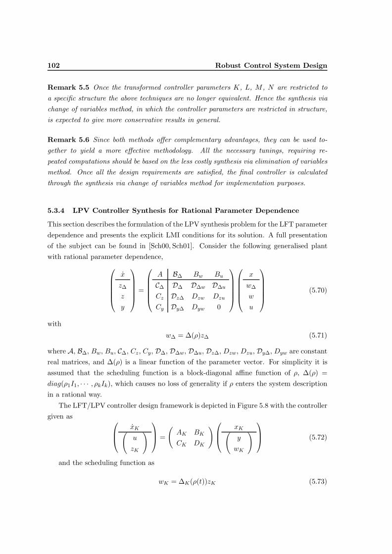
102 Robust Control System Design
Remark 5.5 Once the transformed controller parameters K, L, M , N are restricted toa specific structure the above techniques are no longer equivalent. Hence the synthesis viachange of variables method, in which the controller parameters are restricted in structure,is expected to give more conservative results in general.
Remark 5.6 Since both methods offer complementary advantages, they can be used to-gether to yield a more effective methodology. All the necessary tunings, requiring re-peated computations should be based on the less costly synthesis via elimination of variablesmethod. Once all the design requirements are satisfied, the final controller is calculatedthrough the synthesis via change of variables method for implementation purposes.
5.3.4 LPV Controller Synthesis for Rational Parameter Dependence
This section describes the formulation of the LPV synthesis problem for the LFT parameterdependence and presents the explicit LMI conditions for its solution. A full presentationof the subject can be found in [Sch00, Sch01]. Consider the following generalised plantwith rational parameter dependence,
x
z∆
z
y
=
A B∆ Bw Bu
C∆ D∆ D∆w D∆u
Cz Dz∆ Dzw Dzu
Cy Dy∆ Dyw 0
x
w∆
w
u
(5.70)
with
w∆ = ∆(ρ)z∆ (5.71)
where A, B∆, Bw, Bu, C∆, Cz, Cy, D∆, D∆w, D∆u, Dz∆, Dzw, Dzu, Dy∆, Dyw are constantreal matrices, and ∆(ρ) is a linear function of the parameter vector. For simplicity it isassumed that the scheduling function is a block-diagonal affine function of ρ, ∆(ρ) =diag(ρ1I1, · · · , ρkIk), which causes no loss of generality if ρ enters the system descriptionin a rational way.
The LFT/LPV controller design framework is depicted in Figure 5.8 with the controllergiven as xK(
u
zK
) =
(AK BK
CK DK
) xK(y
wK
) (5.72)
and the scheduling function as
wK = ∆K(ρ(t))zK (5.73)
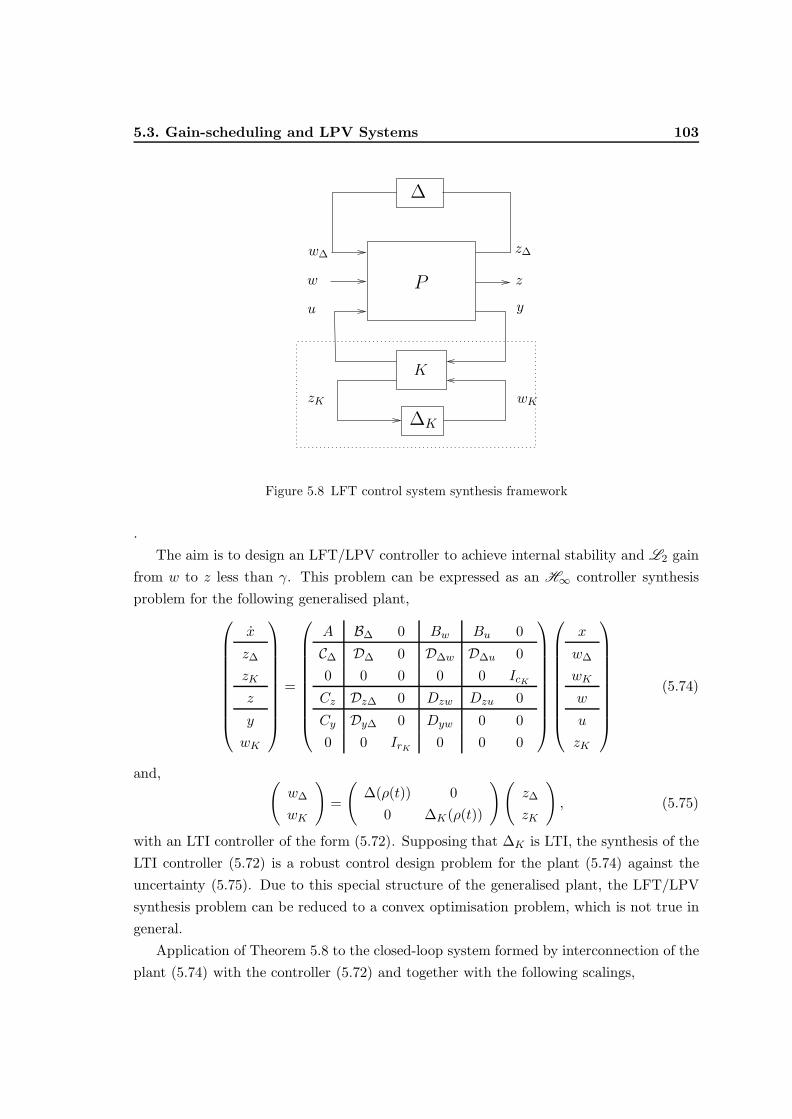
5.3. Gain-scheduling and LPV Systems 103
u
z∆
z
wK
w∆
w
zK
y
K
P
∆
∆K
Figure 5.8 LFT control system synthesis framework
.The aim is to design an LFT/LPV controller to achieve internal stability and L2 gain
from w to z less than γ. This problem can be expressed as an H∞ controller synthesisproblem for the following generalised plant,
x
z∆
zK
z
y
wK
=
A B∆ 0 Bw Bu 0
C∆ D∆ 0 D∆w D∆u 00 0 0 0 0 IcK
Cz Dz∆ 0 Dzw Dzu 0
Cy Dy∆ 0 Dyw 0 00 0 IrK 0 0 0
x
w∆
wK
w
u
zK
(5.74)
and, (w∆
wK
)=
(∆(ρ(t)) 0
0 ∆K(ρ(t))
)(z∆
zK
), (5.75)
with an LTI controller of the form (5.72). Supposing that ∆K is LTI, the synthesis of theLTI controller (5.72) is a robust control design problem for the plant (5.74) against theuncertainty (5.75). Due to this special structure of the generalised plant, the LFT/LPVsynthesis problem can be reduced to a convex optimisation problem, which is not true ingeneral.
Application of Theorem 5.8 to the closed-loop system formed by interconnection of theplant (5.74) with the controller (5.72) and together with the following scalings,

104 Robust Control System Design
P =
(Q S
S′ R
)=
Q1 Q12 S1 S12
Q′12 Q2 S21 S2
S′1 S′21 R1 R12
S′12 S′2 R′12 R2
, (5.76)
P =
(Q S
S′ R
)=
Q1 Q12 S1 S12
Q′12 Q2 S21 S2
S′1 S′21 R1 R12
S′12 S′2 R′12 R2
, (5.77)
where P−1 := P , reveals the main synthesis theorem for the LFT/LPV synthesis.
Theorem 5.11 (LFT/LPV Synthesis) There exists a controller (5.72), a scheduling func-tion (5.73), a symmetric matrix X and a scaling P partitioned as in (5.76) satisfy-ing (5.43), (5.44), (5.45), if and only if there exist partial scalings
P1 =
(Q1 S1
S′1 R1
), withQ1 < 0,
(∆(ρ)I
)′P1
(∆(ρ)I
)> 0, ∀ρ ∈ Γ (5.78)
P1 =
(Q1 S1
S′1 R1
), with R1 > 0,
(I
−∆(ρ)′
)′P1
(I
−∆(ρ)′
)< 0, ∀ρ ∈ Γ (5.79)
and matrices X and Y that satisfy the following conditions(Y I
I X
)> 0 (5.80)
φ′
∗∗∗∗∗∗
′
0 0 0 I 0 00 −γI 0 0 0 00 0 Q1 0 0 S1
I 0 0 0 0 00 0 0 0 1
γ I 0
0 0 S′1 0 0 R1
I 0 00 I 00 0 I
XA XBw XB∆
Cy Dzw Dz∆C∆ D∆w D∆
φ < 0 (5.81)
ψ′
∗∗∗∗∗∗
′
0 0 0 I 0 00 − 1
γ I 0 0 0 0
0 0 Q1 0 0 S1
I 0 0 0 0 00 0 0 0 γI 00 0 S′1 0 0 R1
−Y A′ −Y C ′z −Y C∆
−Bw −D′zw −D′∆w−B′∆ −Dz∆ −D′∆I 0 00 I 00 0 I
ψ < 0 (5.82)
[Det01, Theorem 28], [Sch01, Theorem 4]

5.3. Gain-scheduling and LPV Systems 105
Details of the derivation of the above theorem can be found in [Sch01,Det01]. In the lightof this theorem the general design procedure for the LFT/LPV controller synthesis canbe given as:
i. Find the partial scalings P1, P1 and matrices X and Y that minimise γ under theconstraints (5.78)-(5.82)
ii. Extend the given P1 to the full multiplier P as in (5.76) such that it satisfies∆(ρ) 0
0 ∆K(ρ)
I 00 I
′
P
∆(ρ) 0
0 ∆K(ρ)
I 00 I
> 0 ∀ρ ∈ Γ (5.83)
and such that in its inverse P := P−1 the relevant submatrix is given by P1 asin (5.77) and (5.79)
iii. Then compute the scheduling function ∆K(.) from the constructed full multiplier P .
iv. Compute the controller matrices AK , BK , CK and DK by solving an LMI system.
It has been shown in [Sch01] that the use of the full block scalings P in the above construc-tion leads to a less conservative design in general if compared to the LFT/LPV synthesismethods with the basic or skew-symmetric scalings. However, the controller reconstructionalgorithm for the full block scalings necessitates that ∆K 6= ∆. This leads to a schedulingfunction ∆K that requires the inversion of a large matrix dependent on ρ. It is reportedin [DS01] that this represents a problem in the real-time controller implementation. Forthis reason only the LFT/LPV synthesis methods with basic and skew-symmetric scalingswill be discussed further in the rest of the chapter. Both of these LFT/LPV synthesismethods allow a linear scheduling function ∆K(ρ) = ∆(ρ) = diag(ρ1I1, · · · , ρkIk) for thecontroller, whose implementation requires only simple multiplications. The LFT/LPVsynthesis with basic scalings was first proposed in [Pac94, AG95] and shown to be quiteconservative since it does not take into account the realness of the scheduling parame-ters. The LFT/LPV synthesis with skew-symmetric scalings employs both symmetric andskew-symmetric scalings that take into account the realness of the scheduling parameters.This method was first proposed in [Hel95,SE95]. Although in general the LFT/LPV syn-thesis with skew-symmetric scalings gives more conservative results than the LFT/LPVsynthesis with full block scalings, it is shown in [DS01] that in the case of a one schedulingvariable they are equally conservative.
The following matrices will be used in the exposition of the LMI conditions of bothLFT/LPV synthesis methods

106 Robust Control System Design
ΛX =
XA+A′X + · · ·· · · C′∆R1C∆
XB∆ + C′∆R1D∆ + C′∆S1XBw + · · ·· · · C′∆R1D∆w
C ′z
∗ D′∆R1D∆ −R1 + · · ·· · · D′∆S1 + S′1D∆
D′∆R1D∆w + · · ·· · ·S′1D∆w
D′z∆
∗ ∗ −γI + · · ·· · · D′∆wR1D∆w
D′zw
∗ ∗ ∗ −γI
ΛY =
AY + Y A′ + · · ·· · · B∆R1B′∆
Y C′∆ + B∆R1D′∆ + B∆S1Y C ′z + · · ·· · · B∆R1D′z∆
Bw
∗ D∆R1D′∆ − R1 + · · ·· · · D∆S1 + S′1D′∆
D∆R1D′z∆ + · · ·· · · S′1D′z∆
D∆w
∗ ∗ −γI + · · ·· · · Dz∆R1D′z∆
Dzw
∗ ∗ ∗ −γI
LFT/LPV Synthesis with Basic Scalings
Theorem 5.12 Consider the LPV plant governed by (5.70)-(5.71). There exist a con-troller (5.72), and scheduling function ∆K = ∆ enforcing internal stability and a bound γon the L2 gain of the closed-loop system, whenever there exist symmetric matrices Y andX, and symmetric block-diagonal partial scalings R1, R1 satisfying the following conditions(
Φ 00 I
)′ΛX
(Φ 00 I
)< 0, S1 = 0 (5.84)
(Ψ 00 I
)′ΛY
(Ψ 00 I
)< 0, S1 = 0 (5.85)
(X I
I Y
)> 0,
(R1 I
I R1
)> 0, (5.86)
where Φ, Ψ are any bases of the null spaces of (Cy,Dy∆,Dyw) and (B′u,D′∆u,D′zu) re-spectively. If a solution exists, the LTI part of the LFT/LPV controller can be obtainedas
• Complete X ,
X =
(X U
U ′ E
)=
(Y •• •
)−1
(5.87)

5.3. Gain-scheduling and LPV Systems 107
and scalings as
R =
(R3 R2
R′2 R1
)=
(R3 R2
R′2 R1
)−1
(5.88)
• Solve the following LMI for K =
(AK BK
CK DK
),
ΛK + P ′XclKQcl +Q′clK′PXcl < 0 (5.89)
where
ΛK =
XA+ (∗) A′U 0 XB∆ XBw 0 C′∆ C ′w∗ 0 0 U ′B∆ U ′Bw 0 0 0∗ ∗ −R3 −R2 0 0 0 0∗ ∗ ∗ −R1 0 0 D′∆ D′z∆∗ ∗ ∗ ∗ −γI 0 D′∆w D′zw∗ ∗ ∗ ∗ ∗ −R3 −R2 0∗ ∗ ∗ ∗ ∗ ∗ −R1 0∗ ∗ ∗ ∗ ∗ ∗ ∗ −γI
(5.90)
PXcl =
U ′ E 0 0 0 0 0 0B′uX B′uU 0 0 0 0 D′∆u D′zu
0 0 0 0 0 I 0 0
(5.91)
Qcl =
0 I 0 0 0 0 0 0Cy 0 0 Dy∆ Dyw 0 0 00 0 I 0 0 0 0 0
(5.92)
LFT/LPV Synthesis with Skew-Symmetric Scalings
Theorem 5.13 Consider the LPV plant governed by (5.70)-(5.71). There exist a con-troller (5.72), and a scheduling function ∆K = ∆ enforcing internal stability and a boundγ on the L2 gain of the closed-loop system, whenever there exist symmetric matrices Y andX, symmetric block-diagonal partial scalings R1, R1, and skew-symmetric block-diagonalpartial scalings S1, S1 satisfying the following conditions(
Φ 00 I
)′ΛX
(Φ 00 I
)< 0 (5.93)
(Ψ 00 I
)′ΛY
(Ψ 00 I
)< 0 (5.94)

108 Robust Control System Design
(X I
I Y
)> 0, R1 > 0, R1 > 0, (5.95)
where Φ, Ψ are any bases of the null spaces of (Cy,Dy∆,Dyw) and (B′u,D′∆u,D′zu) re-spectively. If a solution exists, the LTI part of the LFT/LPV controller can be obtainedas
• Construction of the full scalings [DS01]: Choose Q1 = −R1, Q1 = −R1 and form
P1, P1. Define NP := (P1 − P−11 )−1, and Z =
(0I
). Calculate T ,
T :=
(−T2 T12
−T12 T2
), (5.96)
such that (T ′12
T2
)′(NP − Z(Z ′P1Z)−1Z ′)
(T ′12
T2
)> 0. (5.97)
In geometric terms this means that (T ′12 T′2) should be chosen such that its columns
span a positive subspace of (NP −Z(Z ′P1Z)−1Z ′) of half of the dimension of the sizeNP . Obtain PP as,
PP :=
(P1 T
T ′ T ′NPT
)=
(P1 •• •
)−1
(5.98)
Finally form P according to the following partition of PP
PP =
Q1 S1 Q12 S12
S′1 R1 S′12 R12
Q′12 S21 Q2 S2
S′21 R′12 S′2 R2
(5.99)
• Calculate the transformed controller parameters,
K =
K L1 L2
M1 N11 N12
M2 N21 N22
(5.100)
as a solution of the following LMI condition,[ΓK123 ΓK4 ΓK5 ΓK6 ΓK78
]< 0 (5.101)
where R =
(R1 R12
R′12 R2
)= T ′pTp with Tp =
(T1 T12
T ′21 T2
)and matrices ΓKi defined as
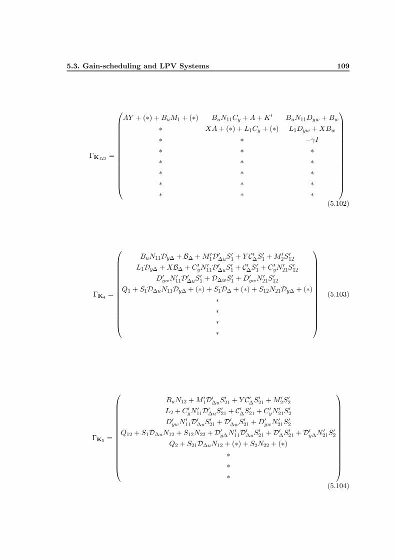
5.3. Gain-scheduling and LPV Systems 109
ΓK123 =
AY + (∗) +BuM1 + (∗) BuN11Cy +A+K ′ BuN11Dyw +Bw
∗ XA+ (∗) + L1Cy + (∗) L1Dyw +XBw
∗ ∗ −γI∗ ∗ ∗∗ ∗ ∗∗ ∗ ∗∗ ∗ ∗∗ ∗ ∗
(5.102)
ΓK4 =
BuN11Dy∆ + B∆ +M ′1D′∆uS′1 + Y C′∆S′1 +M ′2S′12
L1Dy∆ +XB∆ + C ′yN′11D′∆uS′1 + C′∆S′1 + C ′yN
′21S′12
D′ywN′11D′∆uS′1 +D∆wS
′1 +D′ywN
′21S′12
Q1 + S1D∆uN11Dy∆ + (∗) + S1D∆ + (∗) + S12N21Dy∆ + (∗)∗∗∗∗
(5.103)
ΓK5 =
BuN12 +M ′1D′∆uS′21 + Y C′∆S′21 +M ′2S′2
L2 + C ′yN′11D′∆uS′21 + C′∆S′21 + C ′yN
′21S′2
D′ywN′11D′∆uS′21 +D′∆wS′21 +D′ywN
′21S′2
Q12 + S1D∆uN12 + S12N22 +D′y∆N′11D′∆uS′21 +D′∆S′21 +D′y∆N
′21S′2
Q2 + S21D∆uN12 + (∗) + S2N22 + (∗)∗∗∗
(5.104)
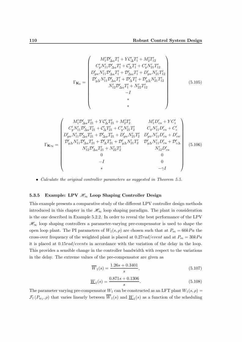
110 Robust Control System Design
ΓK6 =
M ′1D′∆uT ′1 + Y C′∆T ′1 +M ′2T′12
C ′yN′11D′∆uT ′1 + C′∆T ′1 + C ′yN
′21T′12
D′ywN′11D′∆uT ′1 +D′∆wT ′1 +D′ywN
′21T′12
D′y∆N′11D′∆uT ′1 +D′∆T ′1 +D′y∆N
′21T′12
N ′12D′∆uT ′1 +N ′22T′12
−I∗∗
(5.105)
ΓK78 =
M ′1D′∆uT ′21 + Y C′∆T ′21 +M ′2T′2 M ′1D
′zu + Y C ′z
C ′yN′11D′∆uT ′21 + C′∆T ′21 + C ′yN
′21T′2 CyN
′11D
′zu + C ′z
D′ywN′11D′∆uT ′21 +D′∆wT ′21 +D′ywN
′21T′2 D′ywN
′11D
′zu +D′zw
D′y∆N′11D′∆uT ′21 +D′∆T ′21 +D′y∆N
′21T′2 D′y∆N
′11D
′zu +D′z∆
N ′12D′∆uT ′21 +N ′22T′2 N ′12D
′zu
0 0−I 0∗ −γI
(5.106)
• Calculate the original controller parameters as suggested in Theorem 5.5.
5.3.5 Example: LPV H∞ Loop Shaping Controller Design
This example presents a comparative study of the different LPV controller design methodsintroduced in this chapter in the H∞ loop shaping paradigm. The plant in considerationis the one described in Example 5.2.2. In order to reveal the best performance of the LPVH∞ loop shaping controllers a parameter-varying pre-compensator is used to shape theopen loop plant. The PI parameters of W1(s, ρ) are chosen such that at Pm = 60kPa thecross-over frequency of the weighted plant is placed at 0.27rad/event and at Pm = 30kPait is placed at 0.15rad/events in accordance with the variation of the delay in the loop.This provides a sensible change in the controller bandwidth with respect to the variationsin the delay. The extreme values of the pre-compensator are given as
W 1(s) =1.26s + 0.3401
s, (5.107)
W 1(s) =0.871s + 0.1306
s. (5.108)
The parameter varying pre-compensatorW1 can be constructed as an LFT plantW1(s, ρ) =Fl (Pw1 , ρ) that varies linearly between W 1(s) and W 1(s) as a function of the scheduling
5.3. Gain-scheduling and LPV Systems 111
Number ofMethod
LinearisationDecision ρ εlpv
Time1
TechniqueVariables
LMIs (s)
LFT1 - 55 4 0.2056 0.48LFT2 - 61 5 0.2506 0.61
elimi. of var. 43 123˙|ρ| ≤ ∞
0.2506 19.3LPV1
chang. of var. 92 42 0.2394 34.8
elimi. of var.X = X(ρ), Y = Y (ρ) 85 205 0.2657 77.7X = X0, Y = Y (ρ) 64 205 0.2558 55.4
LPV2X = X(ρ), Y = Y0 64 205
˙|ρ| ≤ 0.60.2597 54.2
chang. of var.X = X(ρ), Y = Y0 162 123 0.2593 355.4
Table 5.1 Properties of the different LPV controller synthesis methods applied to a simplified AFRpath model. LFT1 denotes the LFT/LPV synthesis method with basic scalings; LFT2 denotesLFT/LPV synthesis method with skew-symmetric scalings; LPV1 denotes the Grid/LPV methodwith a single Lyapunov function; LPV2 denotes the Grid/LPV method with a parameter-dependentLyapunov function. For the Grid/LPV methods the grid length is chosen as 0.05 for |δ| ≤ 1
parameter (normalised manifold pressure). The post-compensator is chosen as before,
W2(s) =1.5
s+ 1.5. (5.109)
The overall weighted plant can be expressed as,
Gs = W2GW1
= W2Fl (P, ρI2)Fl (Pw1 , ρ)
= Fu (Ps,∆) , (5.110)
with ∆ = ρI3 and four states. Note that the LTI robust stability margin of the weightedplant at its extreme values is εlti = 0.379 and εlti = 0.405 for Pm = 60kPa and Pm = 30kParespectively.
Table 5.1 reveals many important properties of the different LPV controller synthesismethods. The number of decision variables, number of LMIs and computation times areonly given for the LMI conditions that need to be solved in order to compute the L2
gain γ (= ε−1lpv) of the closed-loop system without considering the extra LMIs required for
controller construction. Some important implications are:
• Among the methods that search for a single Lyapunov function (LFT1, LFT2,LPV1), the LFT/LPV synthesis with skew-symmetric scalings (LFT2) is the most

112 Robust Control System Design
attractive one since it is much less conservative than the LFT1 method and alsosignificantly more computationally attractive than the LPV1 method.
• Both the LFT2 and LPV1 method with the elimination of variables technique givethe same value of εlpv without any conservatism. However, when the LPV1 methodwith change of variables technique is employed, the achieved value of εlpv smaller,i.e. conservative as expected.
• The LPV2 method which searches for a parameter-dependent Lyapunov function,gives the best value of the εlpv. The price paid for this is the high computationalcost as the number of decision variables and LMIs are significantly higher for thismethod.
As far as the computation time is concerned it can be seen that the number of decisionvariables is much more costly than the number of LMIs (number of decision variables andLMIs are defined according to the notation of [GNLC95]). For example, in the LPV1method computing the achievable εlpv with the change of variables technique takes moretime than computing it with the elimination of variables technique even though the latterhas a larger number of LMIs.
Figure 5.9 shows the achieved εlti plots by each LPV H∞ controllers together withthe εlti plot achieved by the LTI H∞ controller of Example 5.2.2 for the frozen values of|ρ| ≤ 1. It can be seen that the value of the LPV robust stability margin εlpv is a lowerbound for the εlti plot of an LPV controller, i.e. for a given LPV controller the εlti achievedfor a frozen value of ρ is always greater or equal to the εlpv value of the LPV system.
Figure 5.10 shows the step disturbance rejection performance of the controllers whenthe scheduling parameter varies sinusoidally as depicted in Figure 5.11. An output stepdisturbance at event 5 and an input step disturbance at event 45 are applied to theclosed-loop system. Although all of the controllers perform satisfactorily, the Erms values(root-mean-square (RMS) regulation error at the output) reveal that the ones with betterεlpv values perform better. Note that the LPV2 and LFT2 controllers are the best andsecond-best performers in terms of the Erms performance respectively.
5.4 Comments
The H∞ loop shaping design paradigm and a review of the LPV controller design methodshave been presented in this chapter. The H∞ loop shaping design has been applied toa variety of practical problems, such as flight control [Hyd91,Pap98] and automotive idle
1on an Athlon 1800+ PC with 1GB memory

5.4. Comments 113
−1 −0.8 −0.6 −0.4 −0.2 0 0.2 0.4 0.6 0.8 10.15
0.2
0.25
0.3
0.35
0.4
0.45
0.5LTI LFT1LFT2LPV1LPV2
ρ
Robust
Sta
bil
ity
Marg
inε l
ti
Figure 5.9 LTI robust stability margin for the frozen values of ρ
0 10 20 30 40 50 60 70 80−1
−0.5
0
0.5
1
1.5
Pla
nt O
utpu
t y
events
Erms=4.4154Erms=4.4276Erms=4.1026Erms=4.2004Erms=3.9711
0 10 20 30 40 50 60 70 80−2
−1.5
−1
−0.5
0
0.5
Con
trol
ler
Out
put u
events
LTI LFT1LFT2LPV1LPV2
Figure 5.10 Disturbance rejection performances of the H∞ loop shaping controllers

114 Robust Control System Design
0 10 20 30 40 50 60 70 80−1
−0.8
−0.6
−0.4
−0.2
0
0.2
0.4
0.6
0.8
1
Nor
mal
ised
Sch
edul
ing
Par
amet
er ρ
events
Figure 5.11 Variation of the normalised scheduling parameter
speed control [For00], and found to be performing well. The LPV controller design methodshave been developed recently and are still an area of ongoing research. Although the reviewof the LPV methods in this chapter is not exhaustive, it is rather comprehensive. Moreover,a detailed comparison of the LFT/LPV and Grid/LPV controller design methods havebeen given through the design study presented in Example 5.3.5.
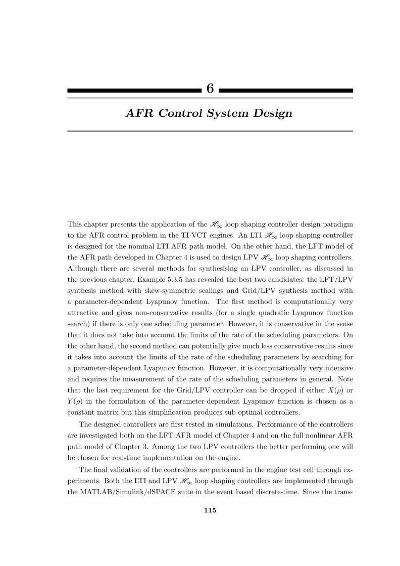
6
AFR Control System Design
This chapter presents the application of the H∞ loop shaping controller design paradigmto the AFR control problem in the TI-VCT engines. An LTI H∞ loop shaping controlleris designed for the nominal LTI AFR path model. On the other hand, the LFT model ofthe AFR path developed in Chapter 4 is used to design LPV H∞ loop shaping controllers.Although there are several methods for synthesising an LPV controller, as discussed inthe previous chapter, Example 5.3.5 has revealed the best two candidates: the LFT/LPVsynthesis method with skew-symmetric scalings and Grid/LPV synthesis method witha parameter-dependent Lyapunov function. The first method is computationally veryattractive and gives non-conservative results (for a single quadratic Lyapunov functionsearch) if there is only one scheduling parameter. However, it is conservative in the sensethat it does not take into account the limits of the rate of the scheduling parameters. Onthe other hand, the second method can potentially give much less conservative results sinceit takes into account the limits of the rate of the scheduling parameters by searching fora parameter-dependent Lyapunov function. However, it is computationally very intensiveand requires the measurement of the rate of the scheduling parameters in general. Notethat the last requirement for the Grid/LPV controller can be dropped if either X(ρ) orY (ρ) in the formulation of the parameter-dependent Lyapunov function is chosen as aconstant matrix but this simplification produces sub-optimal controllers.
The designed controllers are first tested in simulations. Performance of the controllersare investigated both on the LFT AFR model of Chapter 4 and on the full nonlinear AFRpath model of Chapter 3. Among the two LPV controllers the better performing one willbe chosen for real-time implementation on the engine.
The final validation of the controllers are performed in the engine test cell through ex-periments. Both the LTI and LPV H∞ loop shaping controllers are implemented throughthe MATLAB/Simulink/dSPACE suite in the event based discrete-time. Since the trans-
115

116 AFR Control System Design
port delays in the loop limit the achievable AFR regulation performance by feedback,further performance improvements are accomplished by including a feedforward elementinto the control systems. The engine tests are repeated for the feedback-plus-feedforwardcontrollers and a comparison between the feedback and feedback-plus-feedforward con-trollers is presented at the end.
6.1 H∞ Loop Shaping Controller Design
The H∞ loop shaping controller design paradigm is an effective method for designingrobust controllers and has been successfully used in a wide variety of applications. AnAFR controller should have good robustness against system uncertainties and also goodperformance against the disturbances. These are usually conflicting requirements and acompromise has to be achieved. In the sequel an LTI H∞ loop shaping controller withgood robustness and performance properties (εlti > 0.3) is designed for the AFR controlproblem. This LTI controller is required to be robust to parameter variations in the AFRpath. Further robustness and performance improvements are achieved by designing LPVcontrollers. The controller designs in this section follow the lines of Example 5.2.2 andExample 5.3.5.
6.1.1 LTI H∞ Loop Shaping Controller
In order to design an LTI H∞ loop shaping controller an LTI system model is required.Such a linear representation of the AFR path is obtained from the LFT model Gφ =Fl (Pφ,∆φ) developed in Chapter 4 by substituting Pm = 50kPa, EVC=10◦ and IVO=−5◦
in ∆φ. This linear model is called the nominal representation of the system. The nominalmodel G0 is a SISO transfer function with 14 states. Since the input to the model is theFPW in micro seconds and the output of the model is the normalised FAR the steadystate gain of the system is much smaller than one. Therefore, as a common practice inloop shaping design , the nominal plant is scaled to have a unity steady state gain with ascaling factor Sg = 4.2573 × 10³. The scaled nominal plant is denoted as
G0 = G0Sg.
The frequency response of the scaled nominal plant is plotted in Figure 6.1. As the systemunder consideration is in the event based discrete-time, the frequency axis is in rad/eventand w = π represents the Nyquist Frequency. The second order Pade based approxi-mation of the delay introduces RHP zeros at frequencies 0.94rad/event and 2rad/event.Therefore, for a robust closed-loop system the loop bandwidth must be smaller than0.94rad/event. Good robustness and performance can be achieved by appropriate choices
6.1. H∞ Loop Shaping Controller Design 117
10−2
10−1
100
10−2
10−1
100
101
rad/event
Mag
nitu
te (
Loop
shap
e)
GsG0
K∞Gs
Figure 6.1 Singular values of scaled nominal plant G0, weighted plant Gs and K∞Gs
of the pre- and post-compensators. The pre-compensator W1(s) is chosen as a PI weightas before. The integrator in the W1(s) is necessary to achieve zero steady state error andalso improves the performance by boosting the low frequency gain. The proportional gainis used to reduce the phase lag introduced by the integrator around the cross-over fre-quency. The PI parameters of W1(s), shown in Figure 6.2, are chosen to set the cross-overfrequency of the weighted plant at 0.14rad/event,
W1(s) =1.008s + 0.1411
s. (6.1)
These parameters achieve smooth transition of the loop shape around the cross-over fre-quency. The post-compensator W2(s), depicted in Figure 6.2, is chosen to ensure sufficienthigh frequency noise attenuation,
W2(s) =1
s+ 1. (6.2)
Once the weights are chosen and weighted plant Gs = W2G0W1 is formed, the sub-optimalH∞ loop shaping controller, K∞ can be easily the calculated using the µ-tools command“ncfsyn(·)” in MATLAB. Note that the K∞ has 16 states, same as the the weighted plant.The K∞ produces a robust stability margin εlti = 0.4107 for the closed-loop and alsoachieves εlti ≥ 0.25 for all the frozen values of the normalised MAP |ρ| ≤ 1 as it will beshown in Figure 6.4. The final controller K, which has 18 states, can be implemented asK = W1K∞W2, where W1 = SgW1.

118 AFR Control System Design
10−2
10−1
100
100
101
rad/event
Mag
nitu
te (
Wei
ghts
)
W1
W2
Figure 6.2 H∞ loop shaping weights
6.1.2 LPV H∞ Loop Shaping Controller
The LFT approximation of the AFR path can be used to design LPV controllers. Recallthat the LFT model
Gφ = Fl (Pφ,∆φ) , (6.3)
where Pφ ∈ R30×30, ∆φ =diag[PmI5, EVCI5,IVOI5] ∈ R15×15 has 3 scheduling parameters.Designing an LPV controller with 3 scheduling parameters would be computationallyinfeasible with the available LMI solvers. For this reason the LPV controllers are onlydesigned for the MAP variations and the nominal values of the valve timings EVC=10◦
and IVO=−5◦ are substituted in ∆φ. Note that since MAP causes significant variationsin the transport delay and cylinder MAF in the AFR path, it is aimed that the controllerspeed can be varied with respect to the MAP. The resulting LFT model is denoted as
Gpφ = Fl(P pφ ,∆
pφ
)(6.4)
where P pφ ∈ R20×20 has 14 states, 6 inputs and 6 outputs, and ∆pφ = PmI5 ∈ R5×5. In
order to reveal the best performance of the LPV H∞ loop shaping controllers a parameter-varying pre-compensator is designed to shape the open-loop plant. The PI parameters ofW1(s, ρ) (ρ denotes the normalised MAP) is chosen such that at Pm = 70kPa the cross-over frequency of the weighted plant is placed at 0.18rad/event and at Pm = 30kPa itis placed at 0.13rad/events in accordance with the variation of the transport delay inthe loop. This provides sensible variation of the controller bandwidth with respect to thevariations in the delay. The extreme values of the pre-compensator and scaling are given

6.1. H∞ Loop Shaping Controller Design 119
asW 1(s) =
1.13s + 0.2033s
and Sg = 6.0736 × 10³ (6.5)
W 1(s) =1.035s + 0.1346
sand Sg = 3.2772 × 10³ (6.6)
The scaled parameter-varying pre-compensator W1 = W1Sg is constructed as an LFTmodel that varies linearly between W 1Sg and W 1Sg as a function of the normalised MAP
W1 = Fl (Pw, ρ) , Pw ∈ R3×3. (6.7)
The post-compensator is chosen as before,
W2(s) =1
s+ 1. (6.8)
The overall weighted plant can be expressed as an upper LFT,
Gs = Fu (Ps,∆s) , (6.9)
where Ps ∈ R23×23 has 16 states, 7 inputs and 7 outputs, and ∆s = ρI6 ∈ R6×6. Notethat the LTI robust stability margins of the closed-loop system at its extreme values areεlti = 0.38 and εlti = 0.39 for Pm = 70kPa and Pm = 30kPa respectively.
Two different LPV H∞ loop shaping controllers are synthesised for the weighted LFTplant in the following. The first LPV controller is designed via the LFT/LPV synthesismethod with skew-symmetric scalings. The second LPV controller is designed via theGrid/LPV method with a parameter-depending Lyapunov function. In the rest of thischapter ”the LFT controller” will denote the LPV controller designed via the LFT/LPVmethod with skew-symmetric scalings and ”the LPV controller” will denote the LPV con-troller designed via the Grid/LPV method with a parameter-dependent Lyapunov func-tion. Therefore, ”the LPV controller” will refer to the LPV controller designed via theGrid/LPV method but ”the LPV controllers” will refer to both the LFT controller andthe LPV controller. The main advantage of the Grid/LPV method over the LFT/LPVmethod is that it can take into account the rate of variation of the scheduling parameters.Hence, it is important to get realistic estimates of the limits of the rate of the parametervariations in order to compute less conservative LPV controllers.
The global data used for the identification of the wall-wetting dynamics in Section 3.2.5are investigated to obtain some realistic estimates for the limits of the rate of the MAPvariations. Figure 6.3 shows the normalised MAP together with its time derivative inthe event based discrete-time domain. The bottom plot gives an upper bound for thenormalised Pm as ˙|ρ| ≤ 0.065. However, since even more abrupt MAP variations are likelyto occur during engine operation, it is assumed that −0.1 ≤ ρ ≤ 0.1 in the synthesis ofthe LPV controller.
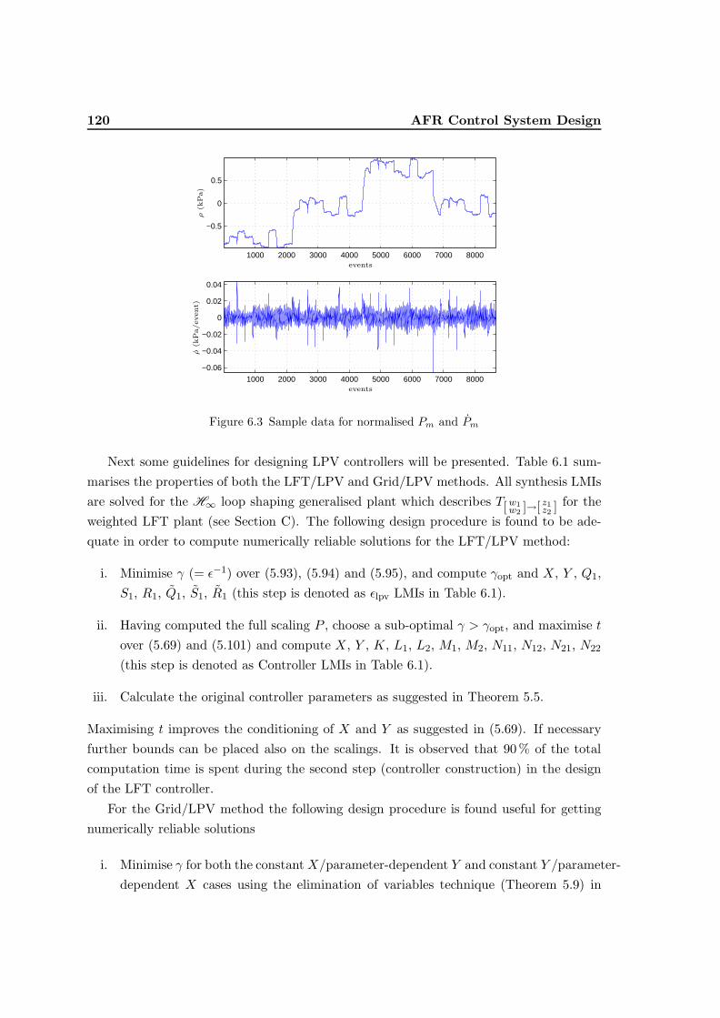
120 AFR Control System Design
1000 2000 3000 4000 5000 6000 7000 8000
−0.5
0
0.5
1000 2000 3000 4000 5000 6000 7000 8000
−0.06
−0.04
−0.02
0
0.02
0.04
ρ(k
Pa)
ρ(k
Pa/event)
events
events
Figure 6.3 Sample data for normalised Pm and Pm
Next some guidelines for designing LPV controllers will be presented. Table 6.1 sum-marises the properties of both the LFT/LPV and Grid/LPV methods. All synthesis LMIsare solved for the H∞ loop shaping generalised plant which describes T[w1
w2 ]→[ z1z2 ] for theweighted LFT plant (see Section C). The following design procedure is found to be ade-quate in order to compute numerically reliable solutions for the LFT/LPV method:
i. Minimise γ (= ε−1) over (5.93), (5.94) and (5.95), and compute γopt and X, Y , Q1,S1, R1, Q1, S1, R1 (this step is denoted as εlpv LMIs in Table 6.1).
ii. Having computed the full scaling P , choose a sub-optimal γ > γopt, and maximise tover (5.69) and (5.101) and compute X, Y , K, L1, L2, M1, M2, N11, N12, N21, N22
(this step is denoted as Controller LMIs in Table 6.1).
iii. Calculate the original controller parameters as suggested in Theorem 5.5.
Maximising t improves the conditioning of X and Y as suggested in (5.69). If necessaryfurther bounds can be placed also on the scalings. It is observed that 90 % of the totalcomputation time is spent during the second step (controller construction) in the designof the LFT controller.
For the Grid/LPV method the following design procedure is found useful for gettingnumerically reliable solutions
i. Minimise γ for both the constant X/parameter-dependent Y and constant Y /parameter-dependent X cases using the elimination of variables technique (Theorem 5.9) in

6.1. H∞ Loop Shaping Controller Design 121
Number ofMethod Notes Decision ρ εlpv Time1
VariablesLMIs (hr)
εlpv LMIs 345 5LFT
Cont. LMIs 802 2˙|ρ| ≤ ∞ 0.2094 0.5
elimi. of var.constant X 409 105 0.2236 8constant Y 409 105 0.2099 8
LPVchang. of var.
˙|ρ| ≤ 0.1
constant X 987 63 0.2236 29(solved twice)
Table 6.1 Comparison of the LPV synthesis methods for AFR controller design. For the Grid/LPVmethod the grid length is chosen as 0.1 for |ρ| ≤ 1
order to find out the less conservative way of dropping the ρ dependence in thecontroller.
ii. For the less conservative case, minimise γ using the change of variables technique(Theorem 5.10) and compute the γopt, K, L, M , N .
iii. (This step is required for improving the conditioning of I−XY ) Choose a sub-optimalγ > γopt, maximise t over (5.69) and the synthesis LMIs given in Theorem 5.10, andcompute K, L, M , N .
iv. Compute AK , BK , CK , DK with the help of (5.58)- (5.61).
Solving the Grid/LPV method via the change of variable technique is much more com-putationally intensive as it can be seen in Table 6.1. It takes around 14.5 hours to solvethe synthesis LMIs with this technique. Since they are solved twice to improve the con-ditioning of I − XY , the total computation time is around 29 hours. This is why mostof the design iterations for the Grid/LPV method should be performed via the elimina-tion of variables techniques which only takes 8 hours of computation time. However, thefinal controller should be computed via the the change of variable technique, since thiscomputes a controller that is more suitable for real-time implementation.
The results show that the use of the Grid/LPV method improves the value of the εlpv =from 0.2094, obtained by the LFT/LPV method, to 0.2236, however at a cost of greatincrease of the computational complexity. Figure 6.4 compares the LTI robust stability
1on an Athlon 1800+ PC with 1GB memory
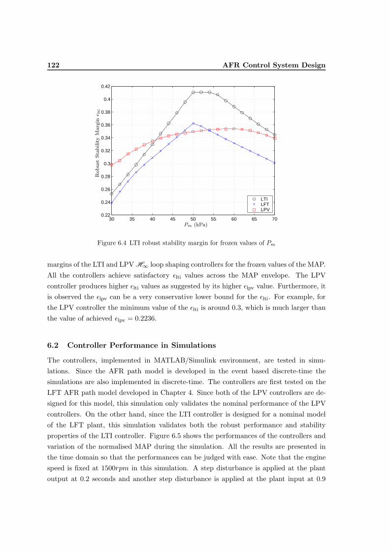
122 AFR Control System Design
30 35 40 45 50 55 60 65 700.22
0.24
0.26
0.28
0.3
0.32
0.34
0.36
0.38
0.4
0.42
LTILFTLPV
Robust
Sta
bil
ity
Marg
inε l
ti
Pm (kPa)
Figure 6.4 LTI robust stability margin for frozen values of Pm
margins of the LTI and LPV H∞ loop shaping controllers for the frozen values of the MAP.All the controllers achieve satisfactory εlti values across the MAP envelope. The LPVcontroller produces higher εlti values as suggested by its higher εlpv value. Furthermore, itis observed the εlpv can be a very conservative lower bound for the εlti. For example, forthe LPV controller the minimum value of the εlti is around 0.3, which is much larger thanthe value of achieved εlpv = 0.2236.
6.2 Controller Performance in Simulations
The controllers, implemented in MATLAB/Simulink environment, are tested in simu-lations. Since the AFR path model is developed in the event based discrete-time thesimulations are also implemented in discrete-time. The controllers are first tested on theLFT AFR path model developed in Chapter 4. Since both of the LPV controllers are de-signed for this model, this simulation only validates the nominal performance of the LPVcontrollers. On the other hand, since the LTI controller is designed for a nominal modelof the LFT plant, this simulation validates both the robust performance and stabilityproperties of the LTI controller. Figure 6.5 shows the performances of the controllers andvariation of the normalised MAP during the simulation. All the results are presented inthe time domain so that the performances can be judged with ease. Note that the enginespeed is fixed at 1500rpm in this simulation. A step disturbance is applied at the plantoutput at 0.2 seconds and another step disturbance is applied at the plant input at 0.9

6.2. Controller Performance in Simulations 123
0 0.5 1 1.5 2
−1
−0.5
0
0.5
1 Erms=5.793 Erms=5.312 Erms=5.3157
0 0.5 1 1.5 2−10000
−8000
−6000
−4000
−2000
0
2000
LTILFTLPV
0 0.5 1 1.5 270
60
50
40
30
Pm
(kP
a)
FP
Wλ
time (s)
time (s)
time (s)
Figure 6.5 Performance of the controllers on the LFT model
seconds. Recall that ”Erms” denotes the RMS regulation error at the plant output. Thesimulation results imply that the LTI controller is robust against the parameter variationsin the model up to ˙|ρ| ≤ 0.06. This also verifies the fact that εlti = 0.41 is a good indicationof the robust performance and stability. Furthermore, the LPV controllers perform betterunder the fast parameter variations as indicated by their εlpv ≥ 0.2. However, nothing canbe said about their robustness properties at this stage since the LFT model is the nominalmodel for the LPV controllers.
In the next simulation, the controllers are tested on the full nonlinear AFR path modelidentified in Chapter 3. Neither the Pade based approximations of the delay nor the affineapproximation of the cylinder MAF model are present in this simulation. Therefore, thefollowing simulation will validate, up to a degree, the robust performance and stability of

124 AFR Control System Design
the LPV controllers as well as those of the LTI controller. A more realistic disturbancetrajectory is designed for this simulation where all the disturbances for the AFR path, i.e.TP, EVC and IVO are excited. The engine speed is constant at 1500rpm for this simula-tion. Figure 6.6 shows the lambda regulation performances of the controllers together withthe FPW, MAP, IVO and EVC traces. As MAP varies between the low and high loads,the valve timings are moved accordingly in some predetermined trajectories. The overlapis reduced to zero at very low loads and increased at mid and high loads. Plots showthat all the H∞ loop shaping controllers perform well under this aggressive disturbancescenario. Moreover, the LPV controllers improve the RMS performance levels almost upto 50%. It is also observed that the LFT and LPV controllers achieve almost the sameRMS performances even though the LPV controller has a slightly higher εlpv value.
The simulations indicate that the designed controllers have the desired robustness andperformance properties not only against the parameter variations but also against theuncertainties in the model.
6.3 Controller Performance in Experiments
Although the simulations indicate good performance of the designed controllers, the finalvalidation of the controllers can only be performed on the real engine. Only one of theLPV controllers is tested on the engine for the following reasons:
Real-time implementation: The LFT controller has important advantages for the real-time implementation since 1) It requires only an LFT operation to get the state spacematrices of the LFT controller at each sampling time 2) Due to its LFT structure its statespace matrices can be discretised off-line. On the other hand, the LPV controller requires1) computation of (5.58), (5.59), (5.60) , (5.61) at each sampling time 2) discretisation ofthe state space matrices of the controller at each sampling time. Therefore, it requiresmuch less computing power to implement the LFT controller in real-time.
Performance: Although the LPV controller has a slightly better εlpv value than thatof the LFT controller, the simulations have not shown that this leads to a performanceimprovement for the LPV controller.
For the above reasons the LFT/LPV controller is chosen for the engine tests togetherwith the LTI controller.

6.3. Controller Performance in Experiments 125
0 5 10 15 20
0.8
1
1.2
Erms=0.39387Erms=0.22157Erms=0.2237
0 5 10 15 20
3000
4000
5000LTILFTLPV
0 5 10 15 20
40
50
60
0 5 10 15 20
05
10
1520
0 5 10 15 20
−20
−10
0
IVO
(◦ATDC
)EVC
(◦ATDC
)Pm
(kPa)
FP
W(µ
s)λ
time (s)
time (s)
time (s)
time (s)
time (s)
Figure 6.6 A realistic disturbance rejection test on the nonlinear model
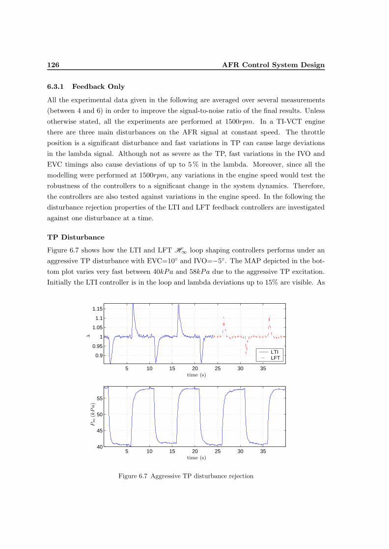
126 AFR Control System Design
6.3.1 Feedback Only
All the experimental data given in the following are averaged over several measurements(between 4 and 6) in order to improve the signal-to-noise ratio of the final results. Unlessotherwise stated, all the experiments are performed at 1500rpm. In a TI-VCT enginethere are three main disturbances on the AFR signal at constant speed. The throttleposition is a significant disturbance and fast variations in TP can cause large deviationsin the lambda signal. Although not as severe as the TP, fast variations in the IVO andEVC timings also cause deviations of up to 5 % in the lambda. Moreover, since all themodelling were performed at 1500rpm, any variations in the engine speed would test therobustness of the controllers to a significant change in the system dynamics. Therefore,the controllers are also tested against variations in the engine speed. In the following thedisturbance rejection properties of the LTI and LFT feedback controllers are investigatedagainst one disturbance at a time.
TP Disturbance
Figure 6.7 shows how the LTI and LFT H∞ loop shaping controllers performs under anaggressive TP disturbance with EVC=10◦ and IVO=−5◦. The MAP depicted in the bot-tom plot varies very fast between 40kPa and 58kPa due to the aggressive TP excitation.Initially the LTI controller is in the loop and lambda deviations up to 15% are visible. As
5 10 15 20 25 30 35
0.9
0.95
1
1.05
1.1
1.15
LTILFT
5 10 15 20 25 30 3540
45
50
55
Pm
(kPa)
λ
time (s)
time (s)
Figure 6.7 Aggressive TP disturbance rejection
6.3. Controller Performance in Experiments 127
soon as the LFT controller is switched on at around 24secs, the peak of the lambda devia-tions are almost cut by half. Note that such a significant improvement in the performanceis achieved without any feedforward action.
A more quantitative comparison of the controllers is given in Figure 6.8. It showsthe RMS performance levels as well as the FPW, MAP and TP traces. This time a lessaggressive but still significant TP disturbance is applied to the AFR loop. The MAPvaries between 38kPa and 49kPa in a square wave manner. The top plot shows that theRMS error is almost halved (50 % improvement) by the LFT controller compared withthat of the LTI controller. The faster response time of the LFT controller is visible in theFPW plot. This is because the LFT controller not only measures the lambda but also theMAP. Therefore, unlike the LTI controller it does not have to wait for the response of thelambda sensor in order to act against a significant variation in the MAP caused by theTP disturbance.
EVC Disturbance
This experiment is performed with constant TP and IVO=−10◦. Figure 6.9 shows the EVCdisturbance rejection performances of the LTI and LFT controllers. The valve overlap waschanged from 0◦ to 30◦ by exciting the EVC timing. Although both controllers performsimilarly, the LTI one has a slightly better performance. This can be analysed from thebehaviour of the MAP shown in the third plot. Consider the first transient, when theMAP increases the gains of the LFT controller are also increased since the increase in theMAP would indicate a shorter transport delay. However, when an increase in the MAPis caused due to an increase in the overlap this would increase the transport delay. Thus,under the EVC excitation the MAP does not capture the dynamics of the system andusing MAP as the scheduling variable misleads the LFT controller. Recall that for thesuccess of the gain-scheduling the scheduling parameter should capture the dynamics ofthe system. Note that the performance of the LFT controller can be further enhanced byscheduling on the EVC timing as well as MAP.
The high frequency noise on the FPW output of the LFT controller can be seen inFigure 6.9. This noise is same as the engine noise present in the MAP measurements.Since the parameters of the LFT controller vary with the MAP, any noise on the MAPsignal immediately affects the output of the LFT controller. This can be prevented byfiltering the MAP measurements before the LFT controller, however this would slow downthe controller response time.
IVO Disturbance
This experiment is performed with fixed TP and EVC=10◦. Figure 6.10 shows the IVOdisturbance rejection performance of the LTI and LFT controllers. The valve overlap was
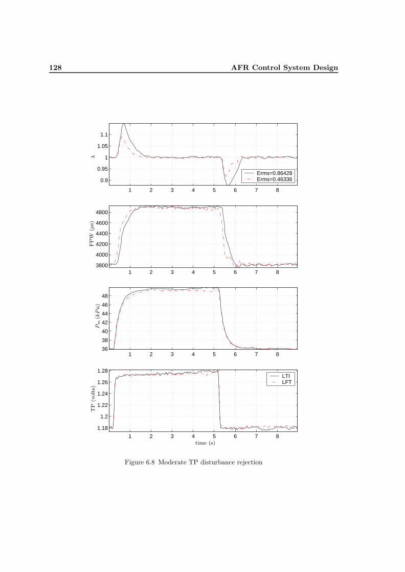
128 AFR Control System Design
1 2 3 4 5 6 7 8
0.9
0.95
1
1.05
1.1
Erms=0.86428Erms=0.46336
1 2 3 4 5 6 7 836
38
40
42
44
46
48
1 2 3 4 5 6 7 83800
4000
4200
4400
4600
4800
1 2 3 4 5 6 7 8
1.18
1.2
1.22
1.24
1.26
1.28LTILFT
Pm
(kPa)
FP
W(µ
s)λ
TP
(volt
s)
time (s)
Figure 6.8 Moderate TP disturbance rejection
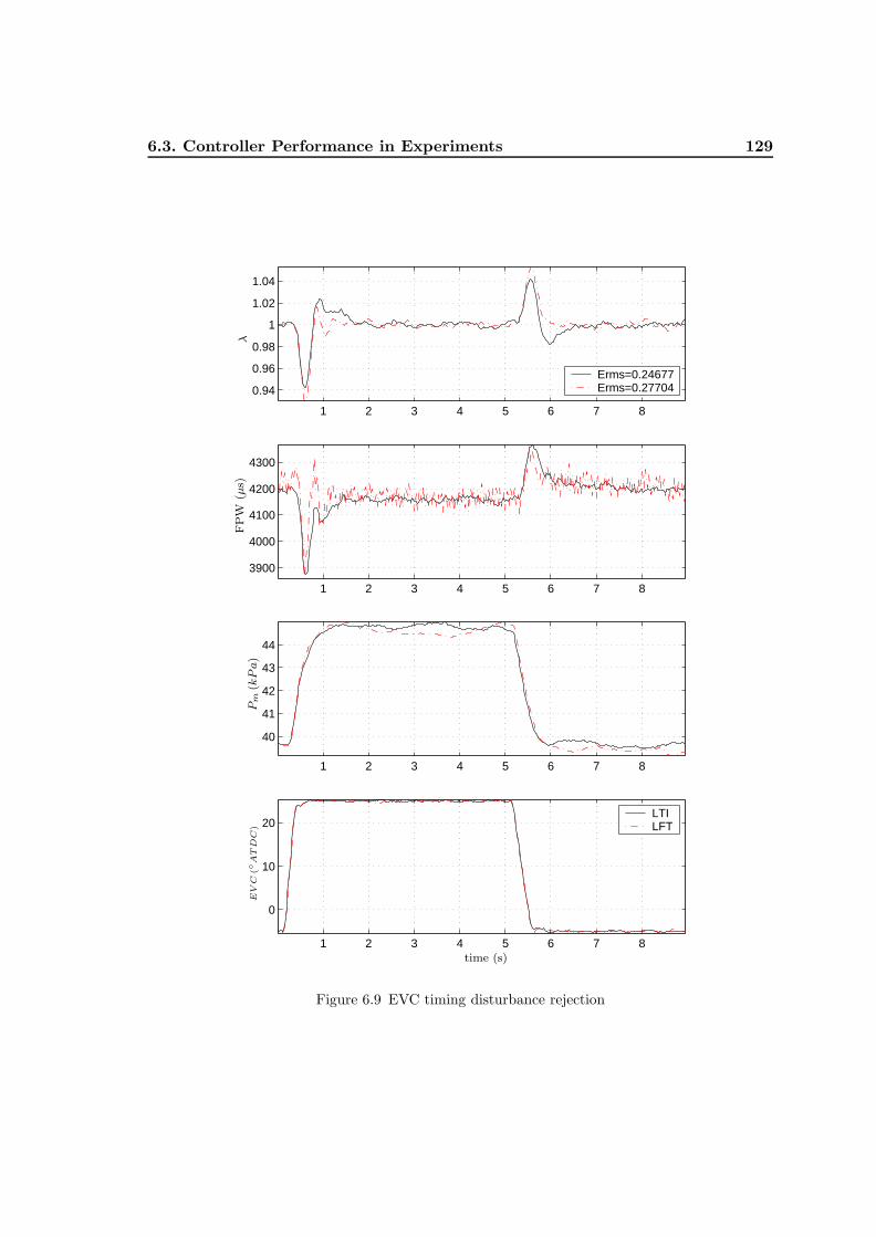
6.3. Controller Performance in Experiments 129
1 2 3 4 5 6 7 8
0.94
0.96
0.98
1
1.02
1.04
Erms=0.24677Erms=0.27704
1 2 3 4 5 6 7 8
40
41
42
43
44
1 2 3 4 5 6 7 8
3900
4000
4100
4200
4300
1 2 3 4 5 6 7 8
0
10
20LTILFT
EVC
(◦ATDC
)Pm
(kPa)
FP
W(µ
s)λ
time (s)
Figure 6.9 EVC timing disturbance rejection

130 AFR Control System Design
1 2 3 4 5 6 7 8
0.96
0.98
1
1.02
1.04
Erms=0.21824Erms=0.19428
1 2 3 4 5 6 7 841
41.5
42
42.5
43
43.5
1 2 3 4 5 6 7 8
4000
4100
4200
4300
4400
1 2 3 4 5 6 7 8
−20
−10
0
10 LTILFT
IVO
(◦ATDC
)Pm
(kPa)
FP
W(µ
s)λ
time (s)
Figure 6.10 IVO timing disturbance rejection

6.3. Controller Performance in Experiments 131
changed from 0◦ to 30◦ by exciting the IVO timing. The achieved RMS errors show thatthis time the LFT controller performs slightly better, although the overall responses ofthe controllers are almost the same. The reason for the better performance of the LFTcontroller is that, the IVO timing affects the MAP in a similar manner to that of the TPexcitation.
Speed Disturbance
This experiment is performed with constant TP, EVC=10◦ and IVO=−5◦. Figure 6.11shows the speed disturbance rejection properties of the LTI and LPV controllers. Theengine speed is varied between 1300 and 1700 rpm through the dynamometer speed controlloop. It is observed that although both controllers can handle the significant variationsin the engine speed with ease, the LFT controller performs 50 % better than the LTIcontroller in terms of the RMS performance. This is because under the speed variationsthe MAP behaves similar to its behaviour under the TP variations for which the LFTcontroller is designed for. Note that such a large improvement in performance is achievedwithout any feedforward action.
6.3.2 Feedback-plus-Feedforward
The above experiments show that both the LTI and LFT controllers have good robustnessproperties. Furthermore, whenever a disturbance affects the AFR path in similar wayto the TP disturbance (such as the engine speed) the LFT controller offers significantimprovements in the RMS performance. However, whenever a disturbance affects theMAP in a way that was not considered during the design of the LFT controller such asthe EVC timing, the LTI controller may perform slightly better. On the other hand,performances of the feedback controllers are limited due to the transport delays present inthe AFR path. Further improvements are possible by introducing a feedforward elementin the AFR control system. It is common practice in the AFR control applications to usethe cylinder MAF estimation in a feedforward sense in order to improve the disturbancerejection performance. However, the cylinder MAF is not the only disturbance acting onthe AFR signal in a TI-VCT engine. Variations in the valve timings also cause significantchanges in the fuel puddle size disturbing the cylinder fuel flow. Therefore, a feedforwardelement should employ not only the air path models but also the wall-wetting model inorder to achieve superior AFR regulation in a TI-VCT engine. The overall structure for afeedback-plus-feedforward controller (also called two degree-of-freedom (2DOF) controller)is depicted in Figure 6.12. Note that in the case of the LFT feedback controller, MAP isalso fed back into the feedback controller.
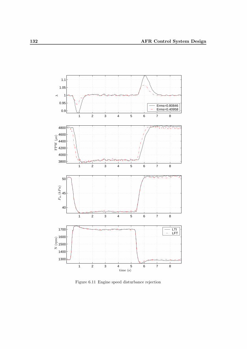
132 AFR Control System Design
1 2 3 4 5 6 7 8
0.9
0.95
1
1.05
1.1
Erms=0.80846Erms=0.40958
1 2 3 4 5 6 7 8
40
45
50
1 2 3 4 5 6 7 83800
4000
4200
4400
4600
4800
1 2 3 4 5 6 7 8
1300
1400
1500
1600
1700 LTILFT
Pm
(kPa)
FP
W(µ
s)λ
time (s)
N(r
pm
)
Figure 6.11 Engine speed disturbance rejection

6.3. Controller Performance in Experiments 133
Feedforward
Feedback
InverseWall−wetting
++
− +
CylinderMAF
Throttleand
Manifold
r
Pm(k) EV C(k) IV O(k)
FPW
TP (k)
Pm(k + 1)mac
λ
uff
ufb
Figure 6.12 Feedback-plus-Feedforward Control System Structure
The feedforward controller is a nonlinear parameter-varying function consisting of thethrottle MAF model (3.2), cylinder MAF model (3.3), manifold pressure model (3.4) andthe inverse of the 4-cylinder wall-wetting model (3.20). The measured values of TP , Pm,IV O and EV C are used to estimate the value of Pm in the next event
Pm(k + 1) = Pm(k) +Kman
(ˆmat(k)− ˆmac(k)
)(6.10)
where Kman = 300 is the manifold gain defined in (3.4). The estimated value Pm(k + 1)is used together with the valve timings to predict the cylinder MAF and fuel puddleparameters in the next event. Note that the feedforward controller does not have anyrobustness properties and its performance is only as good as the accuracy of the modelsused in its design. If the models used are poor, the feedforward action may even degradethe overall performance of the control system. The feedback-plus-feedforward controllersare constructed by combining the LTI and LFT feedback controllers with the feedfor-ward controller as suggested in Figure 6.12 without any modifications. Note that this isa very crude way of designing 2DOF controllers. A more proper way would be to inte-grate the feedforward controller into the H∞ loop shaping design framework and redesignthe feedback controllers to make sure that the feedback and feedforward controller worktogether seamlessly. A well-known guideline for assuring satisfactory performance of a2DOF controller is to make sure that the feedback and feedforward parts are active on dif-ferent frequency ranges. In general feedback controllers are active in the low frequenciesand provide robustness. The feedforward controllers are active at mid-high frequenciesand provide performance. Filtering can be used to decouple the frequency ranges of thecontrollers.
In the following the disturbance rejection tests of Section 6.3.1 are repeated in order

134 AFR Control System Design
to investigate and compare the properties of the 2DOF controllers with the feedback onlycontrollers. In the sequel ”LTI+FF” will denote the 2DOF controller consisting of the LTIH∞ loop shaping feedback controller and the feedforward controller, and ”LFT+FF” willdenote the 2DOF controller consisting of the LFT H∞ loop shaping feedback controllerand the feedforward controller. Note that the LTI+FF and LFT+FF controllers haveexactly the same feedforward controllers.
TP Disturbance
Introducing a well designed feedforward action improves the performance of the controllerssignificantly compared to the feedback only controllers as shown in Figure 6.13. The 2DOFcontrollers perform four times better relative to the LTI controller and two times betterrelative to the LFT controller in terms of the RMS performance. The LTI+FF performsslightly better than the LFT+FF controller. This is because the LTI controller and thefeedforward controller are almost decoupled due to the slow response time of the LTIcontroller. However, since the LFT controller has a much faster response time than theLTI controller, it interacts with the feedforward controller. This interaction reduces theperformance of the LFT+FF controller slightly. However, the robustness guarantees underthe fast parameter variations given by the LFT+FF controller are much greater than thoseof the LTI+FF controller. Superior robustness properties become crucial for the 2DOFcontrollers whenever the feedforward part of the controller produces poor predictions.
EVC Disturbance
This experiment is performed with constant TP and IVO=−10◦. Figure 6.14 shows theEVC disturbance rejection properties of the four controllers. The EVC disturbance rejec-tion capabilities of the feedback controllers are enhanced visibly by the introduction of thefeedforward controller. The peak deviations are reduced from 6 % to 2 % and the RMSerrors are more than halved. As before the LTI+FF controller performs slightly betterthan the LFT+FF controller due to the undesired interaction between the LFT controllerand the feedforward part in the 2DOF control system.
IVO Disturbance
This experiment is performed under constant TP and EVC=10◦. Figure 6.15 shows theIVO disturbance rejection properties of the designed controllers when the valve overlap ischanged from 0◦ to 30◦ via IVO. Significant improvements are achieved in the performanceby the feedforward scheme. Peak deviations are reduced from 4 % to 2 % and the RMSerrors are improved by almost 50 %. Recall that the rapid IVO variations cause changesin the fuel puddle size. The superior performances of the 2DOF controllers are anotherindication that the identified wall-wetting model can predict changes in the fuel puddle

6.3. Controller Performance in Experiments 135
1 2 3 4 5 6 7 8
0.9
0.95
1
1.05
1.1Erms=0.86428Erms=0.46336Erms=0.21961Erms=0.27906
1 2 3 4 5 6 7 8
4000
4500
5000
1 2 3 4 5 6 7 8
40
45
50
1 2 3 4 5 6 7 8
1.18
1.2
1.22
1.24
1.26
1.28 LTI LFT LTI+FFLFT+FF
Pm
(kPa)
FP
W(µ
s)λ
time (s)
TP
(volt
s)
Figure 6.13 TP disturbance rejection (Feedback-plus-Feedforward)
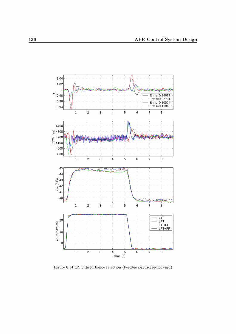
136 AFR Control System Design
1 2 3 4 5 6 7 8
0.94
0.96
0.98
1
1.02
1.04
Erms=0.24677Erms=0.27704Erms=0.10024Erms=0.11043
1 2 3 4 5 6 7 8
3900
4000
4100
4200
4300
4400
1 2 3 4 5 6 7 8
40
41
42
43
44
45
1 2 3 4 5 6 7 8
0
10
20LTI LFT LTI+FFLFT+FF
EVC
(◦ATDC
)Pm
(kPa)
FP
W(µ
s)λ
time (s)
Figure 6.14 EVC disturbance rejection (Feedback-plus-Feedforward)

6.3. Controller Performance in Experiments 137
1 2 3 4 5 6 7 8 9
0.96
0.98
1
1.02
1.04
Erms=0.21824Erms=0.19428Erms=0.0927 Erms=0.12067
1 2 3 4 5 6 7 8 9
4000
4200
4400
1 2 3 4 5 6 7 8 941
42
43
44
1 2 3 4 5 6 7 8 9
−20
−10
0
10 LTI LFT LTI+FFLFT+FF
IVO
(◦ATDC
)Pm
(kPa)
FP
W(µ
s)λ
time (s)
Figure 6.15 IVO disturbance rejection (Feedback-plus-Feedforward)
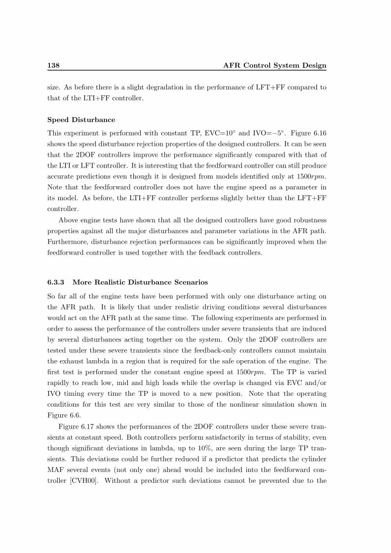
138 AFR Control System Design
size. As before there is a slight degradation in the performance of LFT+FF compared tothat of the LTI+FF controller.
Speed Disturbance
This experiment is performed with constant TP, EVC=10◦ and IVO=−5◦. Figure 6.16shows the speed disturbance rejection properties of the designed controllers. It can be seenthat the 2DOF controllers improve the performance significantly compared with that ofthe LTI or LFT controller. It is interesting that the feedforward controller can still produceaccurate predictions even though it is designed from models identified only at 1500rpm.Note that the feedforward controller does not have the engine speed as a parameter inits model. As before, the LTI+FF controller performs slightly better than the LFT+FFcontroller.
Above engine tests have shown that all the designed controllers have good robustnessproperties against all the major disturbances and parameter variations in the AFR path.Furthermore, disturbance rejection performances can be significantly improved when thefeedforward controller is used together with the feedback controllers.
6.3.3 More Realistic Disturbance Scenarios
So far all of the engine tests have been performed with only one disturbance acting onthe AFR path. It is likely that under realistic driving conditions several disturbanceswould act on the AFR path at the same time. The following experiments are performed inorder to assess the performance of the controllers under severe transients that are inducedby several disturbances acting together on the system. Only the 2DOF controllers aretested under these severe transients since the feedback-only controllers cannot maintainthe exhaust lambda in a region that is required for the safe operation of the engine. Thefirst test is performed under the constant engine speed at 1500rpm. The TP is variedrapidly to reach low, mid and high loads while the overlap is changed via EVC and/orIVO timing every time the TP is moved to a new position. Note that the operatingconditions for this test are very similar to those of the nonlinear simulation shown inFigure 6.6.
Figure 6.17 shows the performances of the 2DOF controllers under these severe tran-sients at constant speed. Both controllers perform satisfactorily in terms of stability, eventhough significant deviations in lambda, up to 10%, are seen during the large TP tran-sients. This deviations could be further reduced if a predictor that predicts the cylinderMAF several events (not only one) ahead would be included into the feedforward con-troller [CVH00]. Without a predictor such deviations cannot be prevented due to the
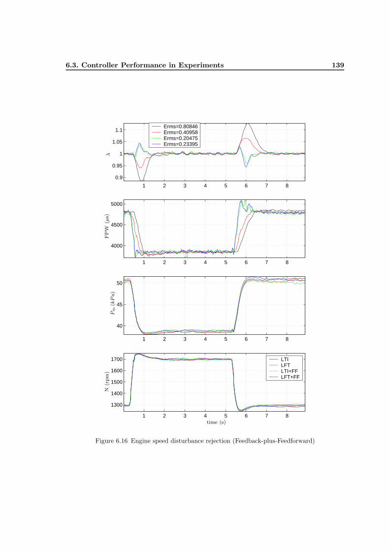
6.3. Controller Performance in Experiments 139
1 2 3 4 5 6 7 8
0.9
0.95
1
1.05
1.1Erms=0.80846Erms=0.40958Erms=0.20475Erms=0.23395
1 2 3 4 5 6 7 8
4000
4500
5000
1 2 3 4 5 6 7 8
40
45
50
1 2 3 4 5 6 7 8
1300
1400
1500
1600
1700 LTI LFT LTI+FFLFT+FF
Pm
(kPa)
FP
W(µ
s)λ
time (s)
N(r
pm
)
Figure 6.16 Engine speed disturbance rejection (Feedback-plus-Feedforward)

140 AFR Control System Design
injection delay in the AFR path. Note that the LTI+FF controller again slightly outper-forms the LFT+FF controller.
A more severe transient scenario is tested repeating the above transient under varyingengine speed conditions. The performances of the controllers are depicted in Figure 6.18.The engine speed takes values between 1300 and 2000rpm in accordance with the TPvariations, i.e. as the TP increases (decreases) the engine speed increases (decreases).Note that the engine speed is controlled by the dynamometer during this test accordingto a predetermined trajectory so this is not an engine test under constant load, i.e. enginespeed is independent of the engine operating conditions. Results are rather interesting:the LFT+FF controller can handle these quite severe transients better than the LTI+FFcontroller. Especially, LFT+FF controller performs better during an unusual transienttaking place around 6.5secs: when the TP moves from 1.21 to 1.27volts, the engine speedrises from 1500 to 2000rpm and the valve timings are advanced, an unusual transient MAPbehaviour occurs. This interesting observation deserves a closer look. Note that since bothcontrollers share exactly the same feedforward parts this difference in performance shouldbe due to a difference between the responses of the feedback parts of the controllers.
In order to check the repeatability of this unusual response the same experiment isrepeated twice. Figure 6.19 shows the controllers’ responses (feedback and feedforwardresponses) and the measured lambda for all of the three experiments. The first rowdisplays the measurements of the first experiment shown in Figure 6.18, second and thirdrow display the second and third experiment respectively. From the feedforward responsesand lambda measurements it can be seen that all three experiments are performed undervery similar conditions even though there is a slight difference between the first and the restof the experiments. This is because the TP is under open loop control only and applyingthe same reference does not lead to the same TP in general. What is certainly common inall of the experiments is that the LFT+FF controller outperforms the LTI+FF controllerin terms of AFR regulation. In order to see the difference in feedback responses of theLTI+FF and LFT+FF controllers, the first column of Figure 6.19 is zoomed in around6.5sec in Figure 6.20. All three measurements suggest that LFT feedback controller canrespond faster during this fast transient without degrading its performance (rapidness ofthe LFT response is more clear in experiments two and three). This supports the view thatthe superior robustness properties of the LFT+FF controller can give it a performancelead whenever there are very fast parameter variations in the system.

6.3. Controller Performance in Experiments 141
2 4 6 8 10 12 14
0.95
1
1.05
1.1 Erms=0.43736Erms=0.48882
2 4 6 8 10 12 14
30
40
50
2 4 6 8 10 12 14
−20
−10
02 4 6 8 10 12 14
0
10
20
2 4 6 8 10 12 143000
4000
5000
2 4 6 8 10 12 14
1.1
1.2
1.3
2 4 6 8 10 12 141400
1500
1600LTI+FFLFT+FF
IVO
(◦ATDC
)EVC
(◦ATDC
)Pm
(kPa)
FP
W(µ
s)λ
time (s)
TP
(volt
s)N
(rpm
)
Figure 6.17 A realistic disturbance rejection test (constant speed)
142 AFR Control System Design
2 4 6 8 10 12 14
0.95
1
1.05
1.1 Erms=0.46695Erms=0.31788
2 4 6 8 10 12 14
30
35
40
45
2 4 6 8 10 12 14
−20
−10
02 4 6 8 10 12 14
0
10
20
2 4 6 8 10 12 14
3000350040004500
2 4 6 8 10 12 141.05
1.11.15
1.21.25
2 4 6 8 10 12 14
1400
1600
1800
2000LTI+FFLFT+FF
IVO
(◦ATDC
)EVC
(◦ATDC
)Pm
(kPa)
FP
W(µ
s)λ
time (s)
TP
(volt
s)N
(rpm
)
Figure 6.18 A realistic disturbance rejection test (varying speed)

6.3. Controller Performance in Experiments 143
5 10 15
−100
0
100
200
300
400
500
600
FEEDBACK RESPONSE
5 10 15
−400
−200
0
200
400
600
5 10 15−500
0
500
5 10 152500
3000
3500
4000
FEEDFORWARD RESPONSE
5 10 15
3000
3500
4000
4500
5 10 15
3000
3500
4000
4500
5 10 15
0.95
1
1.05
1.1LAMBDA
5 10 15
0.9
0.95
1
1.05
1.1
1.15
5 10 15
0.9
0.95
1
1.05
1.1
1.15
FP
W(µ
s)F
PW
(µs)
FP
W(µ
s)
FP
W(µ
s)F
PW
(µs)
FP
W(µ
s)
λλ
λ
time (s)time (s)time (s)
I
I
I
II
II
II
III
III
III
Figure 6.19 Feedback and feedforward responses of the controllers
6 6.1 6.2 6.3 6.4 6.5 6.6 6.7 6.8 6.9 7
−200
0
200
400
FEEDBACK RESPONSE (Zoomed)
6 6.1 6.2 6.3 6.4 6.5 6.6 6.7 6.8 6.9 7−500
0
500
LTI+FFLFT+FF
6 6.1 6.2 6.3 6.4 6.5 6.6 6.7 6.8 6.9 7−500
0
500
FP
W(µ
s)F
PW
(µs)
FP
W(µ
s)
time (s)
I
II
III
Figure 6.20 Feedback responses of the controllers (zoomed)

144 AFR Control System Design
6.4 Comments
The LTI and LFT/LPV H∞ loop shaping controllers have been successfully designedand implemented on a TI-VCT engine for AFR control. The designed controllers haveundergone extensive engine tests under various conditions. The experiments show that theLFT/LPV controller offers significant improvements in the AFR regulation performanceas far as a feedback-only controller is concerned. When complemented with a well designedfeedforward controller both the LTI and LFT controllers (LTI+FF and LFT+FF) performalmost equally well, beating even the performance of the LFT feedback-only controllereasily. However, due to the undesired interactions between the LFT and feedforwardcontroller a slight degradation in the performance is observed for the LFT+FF controller.Although a possible remedy would be to incorporate the feedforward controller into theLFT/LPV controller design framework, this could not be done during this study due tolack of time. On the other hand, the LFT+FF controller is observed to handle an unusualfast transient better than the LTI+FF controller. This might be contributed to the LFTcontroller’s good robustness and performance properties against fast parameter changes.This is the first time an LFT/LPV AFR controller is designed and tested in real-timeon an automotive engine to the author’s knowledge as far as the published literature isconcerned.
Note that since a reduced LFT model (varying only with MAP) of the identifiedAFR path model has been used in this chapter to design the LPV feedback controllers,the feedback synthesis did not take the full advantage of the identification performed inChapter 3. Although it was desirable to use the full knowledge of the system, i.e. scheduleon at least two parameters (MAP, IVO and maybe even EVC), this was not accomplisheddue to lack of time and computation issues as discussed before.
7
Conclusions
Modelling, identification and control of the AFR path in a TI-VCT engine have beeninvestigated in this thesis. The TI-VCT mechanism induced variations in the wall-wettingdynamics have been verified and modelled with the help of gaseous fuel experiments. Boththe LTI and LPV AFR controllers have been designed in the H∞ loop shaping framework.Moreover, they have been implemented on the TI-VCT engine and tested successfully in avariety of different transient conditions. The experimental evaluation of the controllers hasrevealed that the LFT/LPV feedback controller offers up to 50 % improvements in AFRregulation performance compared to that of the LTI controller. Further improvements inthe controllers’ performances have been achieved by including a feedforward controller intothe AFR control systems. The success of the feedforward controller in disturbance rejectionis considered as another indication of the quality of the identified AFR path model. On theother hand it has been observed that when complemented with the feedforward controllerboth the LTI+FF and LFT+FF controllers perform almost equally well. Finally thegood performance of the controllers on the engine without any fine tuning shows that theH∞ loop shaping framework produces high performance robust controllers even for anenvironment as complex and uncertain as the TI-VCT engine as long as a reliable modelis available.
7.1 Main Contributions
A parameter-varying AFR path model. A parameter-varying mean value TI-VCTengine model has been identified for the AFR control problem. An alternative cylinderMAF model has been proposed and identified for VCT engines. Furthermore, it has beenobserved that some nonlinear dynamics such as the wall-wetting in the VCT engine cannotbe identified satisfactorily via linear (local) identification methods.
145

146 Conclusions
An LPV wall-wetting model. Variations in the wall-wetting dynamics under the TI-VCT excitations have been observed with the help of gaseous fuel experiments. A globalidentification framework is proposed for the identification of the wall-wetting dynamicswhich are modelled as a slow and a fast first order fuel puddles. The LPV wall-wettingmodel have been shown to predict the fuel film size variations accurately through validationand also through the good performance of the feedforward controller during the enginetests.
A comprehensive review of the LPV controller design methods. Several differentLPV controller design methods have been presented in a unified and systematic frame-work. Whenever possible coding friendly forms of the LMI conditions are provided forease of numerical implementation of the methods. A detailed comparison of the differentLPV methods is provided through the illustrative examples and design of the final AFRcontrollers.
Design and experimental implementation of the LPV H∞ loop shaping AFR
controllers. The LTI and LPV H∞ loop shaping AFR controllers have been designedand successfully implemented on the TI-VCT engine. It is shown that the LPV controlleroffers significant improvements in the feedback-only performance as long as the schedulingparameter captures the nonlinear dynamics of the system.
7.2 Further Work
Results of this thesis can be further developed and enhanced in several ways:
Expansion of the AFR path model to different engine speeds. The AFR pathmodel has been developed at 1500rpm. Even though the experiments have shown thatthe designed controllers are robust against the variations in the engine speed, furtherimprovements in performance can be realised if the model would also include the enginespeed as a parameter. It is believed that the proposed identification methods can easilybe extended to include the engine speed into the AFR path model.
Enhancement of the LPV controller performance and robustness by scheduling
on two or even three parameters The designed LPV controller is only scheduled onthe MAP. Further improvements in the performance can be achieved if the controller isgain-scheduled with the valve timings as well as the MAP. A second scheduling parameterwould be the IVO timing since it affects the wall-wetting dynamics significantly. If compu-tationally found feasible, the EVC timing can also be included as a scheduling parameter

7.2. Further Work 147
to realise an LPV controller with 3 scheduling parameters. Note that only the LFT/LPVmethods are suitable for design of the LPV controllers with several scheduling parametersdue to the intensive computational requirement of the Grid/LPV methods.
Integration of feedforward controllers into the LPV H∞ loop shaping design
framework. It has been observed that there are some undesired interactions betweenthe feedforward and LPV controller which cause slight degradations in the 2DOF LPVcontroller’s performance. This problem can be alleviated by incorporating the feedforwardcontroller into the LPV H∞ loop shaping design framework.
Designing a MIMO control system that controls not only the AFR but also
the valve timings. Only SISO controllers have been designed in this thesis. Since thereis high interaction between the valve timings and AFR path dynamics, the overall perfor-mance can be further improved if a MIMO control system that controls not only the AFRbut also the valve timings is designed for the TI-VCT engine.


A
Facilities
The Engineering Department at Cambridge University has two state of the art transientengine test cells. These facilities were jointly funded by the Engineering and PhysicalSciences Research Council (EPSRC) and the Ford Motor Company, with approximately65 % of the funding from the latter.
This appendix describes the facilities available in the first of the two cells where theAFR control investigation in a TI-VCT engine was carried out.
A.1 Dynamometer
The dynamometer used in the gasoline cell is a low inertia 103kW d.c. electric motor.The drive unit enables transient capabilities by controlling a fast thyristor bridge networkwhich controls the field and armature currents in the motor. The dynamometer is usedto absorb energy from, or to motor, the engine. Typically the dynamometer will be inspeed control mode. If the engine is generating net positive torque at the reference speedthe dynamometer will absorb energy from the shaft (and generate electricity which is fedback into the grid). Conversely if net negative torque is generated by the engine then thedynamometer will motor the engine to keep the speed at the desired value. The low systeminertia and fast control loop enable relatively fast transient response characteristics.
A.2 Engine
The engine is a prototype Ford TI-VCT 1.6l 16 valve gasoline engine. It is connectedto the dynamometer via a clutch which can be used to accurately duplicate gear changeevents, and also to allow the engine to idle disconnected from the dynamometer.
149
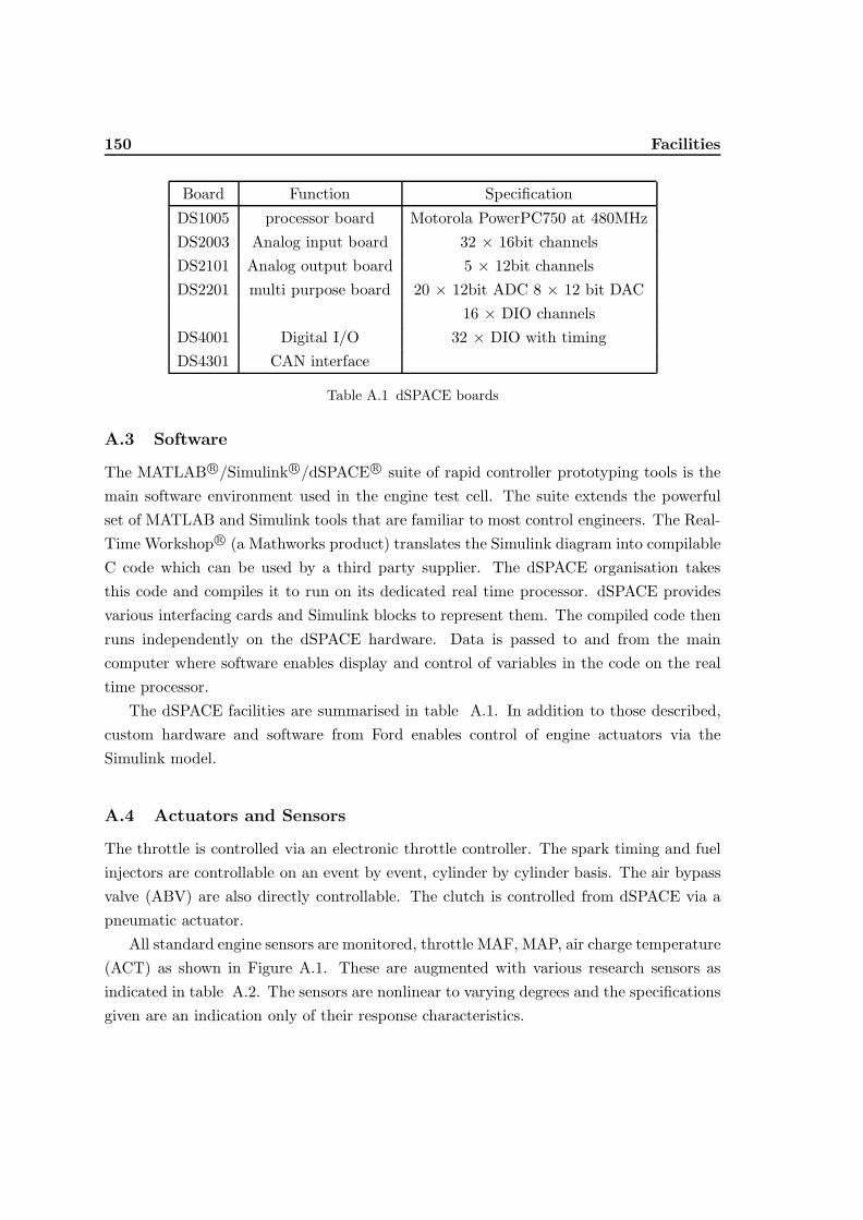
150 Facilities
Board Function Specification
DS1005 processor board Motorola PowerPC750 at 480MHzDS2003 Analog input board 32 × 16bit channelsDS2101 Analog output board 5 × 12bit channelsDS2201 multi purpose board 20 × 12bit ADC 8 × 12 bit DAC
16 × DIO channelsDS4001 Digital I/O 32 × DIO with timingDS4301 CAN interface
Table A.1 dSPACE boards
A.3 Software
The MATLAB r©/Simulink r©/dSPACE r© suite of rapid controller prototyping tools is themain software environment used in the engine test cell. The suite extends the powerfulset of MATLAB and Simulink tools that are familiar to most control engineers. The Real-Time Workshop r© (a Mathworks product) translates the Simulink diagram into compilableC code which can be used by a third party supplier. The dSPACE organisation takesthis code and compiles it to run on its dedicated real time processor. dSPACE providesvarious interfacing cards and Simulink blocks to represent them. The compiled code thenruns independently on the dSPACE hardware. Data is passed to and from the maincomputer where software enables display and control of variables in the code on the realtime processor.
The dSPACE facilities are summarised in table A.1. In addition to those described,custom hardware and software from Ford enables control of engine actuators via theSimulink model.
A.4 Actuators and Sensors
The throttle is controlled via an electronic throttle controller. The spark timing and fuelinjectors are controllable on an event by event, cylinder by cylinder basis. The air bypassvalve (ABV) are also directly controllable. The clutch is controlled from dSPACE via apneumatic actuator.
All standard engine sensors are monitored, throttle MAF, MAP, air charge temperature(ACT) as shown in Figure A.1. These are augmented with various research sensors asindicated in table A.2. The sensors are nonlinear to varying degrees and the specificationsgiven are an indication only of their response characteristics.
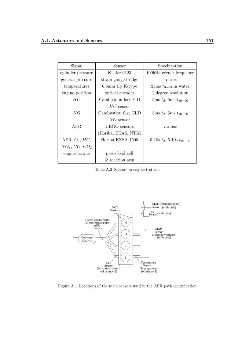
A.4. Actuators and Sensors 151
Signal Sensor Specification
cylinder pressure Kistler 6123 100kHz corner frequencygeneral pressure strain gauge bridge ≈ 1ms
temperatures 0.5mm tip K-type 25ms t0−63 in waterengine position optical encoder 1 degree resolution
HC Cambustion fast FID 5ms td, 5ms t10−90
HC sensorNO Cambustion fast CLD 5ms td, 5ms t10−90
NO sensorAFR UEGO sensors various
(Horiba, ETAS, NTK)AFR, O2, HC, Horiba EXSA 1500 5-10s td, 5-10s t10−90
NOx, CO, CO2
engine torque piezo load cell& reaction arm
Table A.2 Sensors in engine test cell
AFR
3
4
2
1
ConverterCatalytic
TemperatureSensor
SensorMAF
SensorTP
Sensor
SensorsVCT
AFRSensor
(30cm upstream)
(5cm upstream)(of injector1)
(11cm downstream)(of throttle)
(8cm downstream)(of cylinder1)
(of confluence point)(10cm downstream)
(of throttle)
SensorMAP
(at throttle)
Figure A.1 Locations of the main sensors used in the AFR path identification


B
Input Excitations for Linear Identification
In order to have an informative identification data the input should be persistently exciting,i.e. it should contain sufficiently many distinct frequencies. This remains enough freedomfor choice of the input excitation. The common input signals for linear identificationare filtered Gaussian white noise, random binary signals, pseudo-random binary signal(PRBS), multi-sines and chirp signal (swept sinusoids). Two of the above inputs will bedefined in the following.
B.1 PRBS
A PRBS is periodic, deterministic signal with white-noise-like properties. It is generatedby the difference equation
u(t) = rem(A(q)u(t), 2) = rem(a1u(t− 1) + ...+ anu(t− n), 2) (B.1)
Here rem(x,2) is the remainder as x is divided by 2. If the polynomial A(q) is chosensuch that Maximum length PRBS is obtained [Lju99, p. 419], the PRBS has the followingproperties:
• period of the sequence is Tprbs = (2n − 1)Tc where n is the number of registers andTc is period of the clock generating PRBS
• the mean of the PRBS is given by u2n−1 when is its magnitudes shifts between ±u
• Its frequency response has (2n−2)/2 frequency peaks for positive frequencies(excluding0 frequency).
Figure B.1 shows one period of a PRBS with it frequency response. The Nyquistfrequency is labelled as fn = π/Ts. This shows that maximum length PRBS with Ts = Tc
153
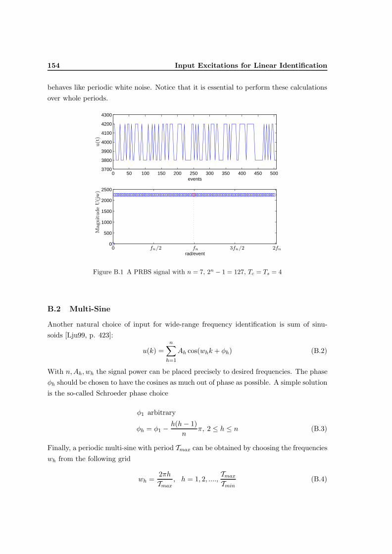
154 Input Excitations for Linear Identification
behaves like periodic white noise. Notice that it is essential to perform these calculationsover whole periods.
0 50 100 150 200 250 300 350 400 450 5003700
3800
3900
4000
4100
4200
4300
events
00
500
1000
1500
2000
2500
rad/eventfnfn/2 3fn/2 2fn
u(t
)M
agnit
ude
U(j
w)
Figure B.1 A PRBS signal with n = 7, 2n − 1 = 127, Tc = Ts = 4
B.2 Multi-Sine
Another natural choice of input for wide-range frequency identification is sum of sinu-soids [Lju99, p. 423]:
u(k) =n∑h=1
Ah cos(whk + φh) (B.2)
With n,Ah, wh the signal power can be placed precisely to desired frequencies. The phaseφh should be chosen to have the cosines as much out of phase as possible. A simple solutionis the so-called Schroeder phase choice
φ1 arbitrary
φh = φ1 −h(h− 1)
nπ, 2 ≤ h ≤ n (B.3)
Finally, a periodic multi-sine with period Tmax can be obtained by choosing the frequencieswh from the following grid
wh =2πhTmax
, h = 1, 2, ....,TmaxTmin
(B.4)

B.2. Multi-Sine 155
Such a periodic input excites Tmax/Tmin equally distanced frequencies between 2π/Tmaxand 2π/Tmin with increments of 2π/Tmax. The main advantage of having a periodic inputis that the signal-to-noise-ratio can be improved by averaging the measurement over theperiod. For the identification tests in this study Tmax = 684 and Tmin = 9 are chosen.
0 100 200 300 400 500 6003700
3800
3900
4000
4100
4200
events
00
2000
4000
6000
8000
rad/eventfn/4 fn/2 3fn/4 fn 5fn/4 3fn/2 7fn/4 2fn
u(t
)M
agnit
ude
U(j
w)
Figure B.2 A multi-sine signal with Tmax = 684, Tmin = 9 and Ts = 1

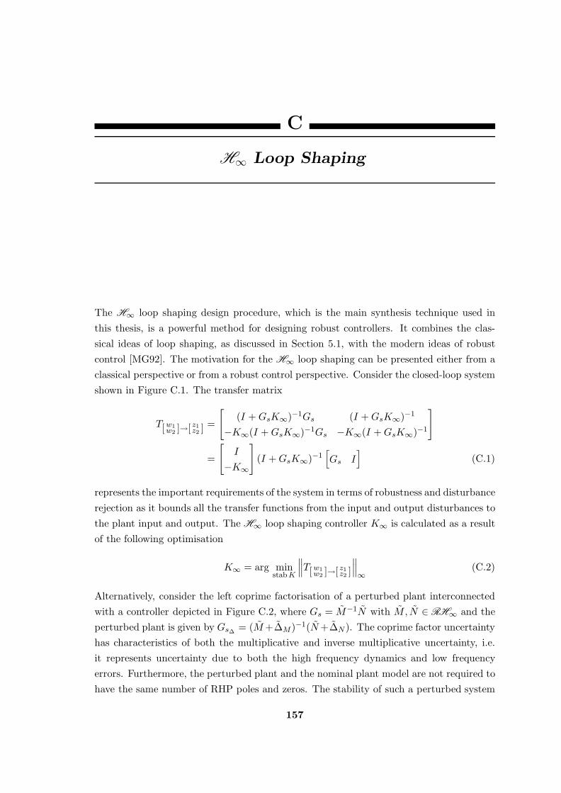
C
H∞ Loop Shaping
The H∞ loop shaping design procedure, which is the main synthesis technique used inthis thesis, is a powerful method for designing robust controllers. It combines the clas-sical ideas of loop shaping, as discussed in Section 5.1, with the modern ideas of robustcontrol [MG92]. The motivation for the H∞ loop shaping can be presented either from aclassical perspective or from a robust control perspective. Consider the closed-loop systemshown in Figure C.1. The transfer matrix
T[w1w2 ]→[ z1z2 ] =
[(I +GsK∞)−1Gs (I +GsK∞)−1
−K∞(I +GsK∞)−1Gs −K∞(I +GsK∞)−1
]
=
[I
−K∞
](I +GsK∞)−1
[Gs I
](C.1)
represents the important requirements of the system in terms of robustness and disturbancerejection as it bounds all the transfer functions from the input and output disturbances tothe plant input and output. The H∞ loop shaping controller K∞ is calculated as a resultof the following optimisation
K∞ = arg minstabK
∥∥∥T[w1w2 ]→[ z1z2 ]
∥∥∥∞
(C.2)
Alternatively, consider the left coprime factorisation of a perturbed plant interconnectedwith a controller depicted in Figure C.2, where Gs = M−1N with M, N ∈ RH∞ and theperturbed plant is given by Gs∆ = (M+∆M)−1(N+∆N ). The coprime factor uncertaintyhas characteristics of both the multiplicative and inverse multiplicative uncertainty, i.e.it represents uncertainty due to both the high frequency dynamics and low frequencyerrors. Furthermore, the perturbed plant and the nominal plant model are not required tohave the same number of RHP poles and zeros. The stability of such a perturbed system
157

158 H∞ Loop Shaping
−
z1z2 w1 w2
W1 W2
Gs
G
K∞
Figure C.1 The H∞ loop shaping typical block diagram
depends on the following transfer function,
Tw→[ z1z2 ] =
[−K∞I
](I +GsK∞)−1M−1. (C.3)
Using a small gain argument it can be shown that the perturbed system is internally stablewith a controller K∞ if and only if∥∥∥∥∥
[−K∞I
](I +GsK∞)−1M−1
∥∥∥∥∥∞< β, given
∥∥∥[∆N ∆M
]∥∥∥∞≤ 1β. (C.4)
The equivalence of these two different approaches can be shown by the following equal-ity [ZDG96, Lemma 18.4]∥∥∥∥∥
[−K∞I
](I +GsK∞)−1M−1
∥∥∥∥∥∞
=
∥∥∥∥∥[
I
−K∞
](I +GsK∞)−1
[Gs I
]∥∥∥∥∥∞
(C.5)
Thus, the H∞ loop shaping optimisation (C.2) produces a controller that has optimaldisturbance properties and is optimally robust to the coprime factor perturbations of theplant. The success of the optimisation can be judged by the value of the robust stabilitymargin ε
ε =∥∥∥T[w1
w2 ]→[ z1z2 ]
∥∥∥−1
∞(C.6)
−∆N ∆M
N M
K∞
z1 z2
w
Figure C.2 Left coprime factor uncertain plant

C.1. McFarlane and Glover’s Design Procedure 159
An H∞ loop shaping design which achieves a robust stability margin ε = ε0 will be robustlystable to coprime factor perturbations in the plant of size
∥∥∥[∆N ∆M
]∥∥∥∞< ε−1
0 . Thevalue of ε is always between 0 and 1, and a value closer to unity indicates a loop shapewhich has good robust stability properties.
C.1 McFarlane and Glover’s Design Procedure
i. For an appropriately scaled system, shape the singular values of the nominal plantG using a pre-compensator W1 and/or a post-compensator W2 to get the desiredloop shape as shown in Figure 5.3. The weighted plant is given by Gs = W2GW1.
ii. Calculate εmax, where
ε−1max = inf
stab K∞
∥∥∥T[w1w2 ]→[ z1z2 ]
∥∥∥∞
(C.7)
If εmax < 0.25 return to 1) and adjust W1 and W2. If εmax > 0.25 select ε ≤ εmax,then synthesise a controller K∞, which satisfies∥∥∥T[w1
w2 ]→[ z1z2 ]
∥∥∥∞≤ ε−1 (C.8)
iii. The final controller K is constructed by combining the H∞ controller K∞ with theweighting matrices W1 and W2 such that K = W1K∞W2.
The theoretical basis for the H∞ loop shaping is that K∞ does not modify the desired loopshape significantly at low and high frequencies, if εmax is not too small. Thus, shaping theopen loop plant G corresponds to shaping the loop gains GK and KG. In contrast withthe conventional loop shaping, the control engineer does not need to shape the phase of Gexplicitly. It can be shown that a value of εmax > 0.2−0.3 is satisfactory, in the same waythat a gain margin of ±6 dB, and phase margin of 45◦ are for a SISO system. If εmax issmall, then the desired loop shape is incompatible with the robust stability requirementsand should be adjusted accordingly (note that the calculation of εmax is routine). It isshown that all the closed-loop objectives are guaranteed to have bounded magnitudes.Moreover, the bounds depend only on εmax, W1, W2 and G (see [ZDG96, Section 18.3]for further discussion).
The most crucial part of the design procedure is to find the appropriate weightingmatrices. The shape of the weights is determined by the closed-loop design specifications.The general trends to be followed are high low frequency gain so that the disturbancerejection at both the input and the output of the plant, as well as output decoupling areachieved; low high frequency gain for noise rejection; and a smooth transition around theloop cross-over frequency, i.e. the loop gain should not decrease faster than 20dB/decade,

160 H∞ Loop Shaping
in order to achieve the desired robust stability and performance such as good gain andphase margins. A fast rise time can be achieved with a high loop cross-over frequencyand a good ε. High low frequency gain can be achieved with a PI weight. Low highfrequency gain can be realized with a low-pass filter. A lead-lag filter can provide thesmooth transition around the loop cross-over frequency.
C.2 ν-Gap Metric
The ν-gap metric indicates how close two systems are to each other in terms of theirclosed-loop behaviour. The distance between two plants as measured by the ν-gap metricis a measure of alikeness of their closed loop behaviour. The gap between two plants G0
and G1 is defined as the smallest value of ‖[∆N ,∆M ]‖∞, coprime factor perturbation, thatperturbs G0 into G1 and is denoted by δν(G0, G1). In this framework the robust stabilitymargin ε gives the radius, in terms of the distance in the gap metric, of the largest ball ofplants stabilised by K as shown in Figure C.3.
by KAll plants stabilised
Largest Ball
G0
εmax
Figure C.3 Interpretation of robust stability margin ε in the gap metric
Theorem C.1 Let G0 be a nominal plant and β ≤ α < εmax.
i. For a given controller K,
arcsinε > arcsinα− arcsin β
for all G satisfying δν(G0, G) ≤ β if and only if ε > α.
ii. For a given plant G,arcsinε > arcsinα− arcsin β
for all K satisfying ε > α if and only if δν(G0, G) ≤ β [Vin99, Theorem 3.10].
The preceding theorem shows that any plant at a distance less than β from the nominalwill be stabilised by any controller stabilising the nominal with a robust stability marginof at least β. Moreover, any plant at a distance greater than β from the nominal will bedestabilised by some controller that stabilises the nominal with a performance measure ofβ.

Bibliography
[AA98] P. Apkarian and R.J. Adams. Advanced Gain-Scheduling Techniques for Un-certain Systems. IEEE Transactions on Control Systems Technology, 6(1):21–32, January 1998.
[AG95] P. Apkarian and P. Gahinet. A Convex Chracterization of Gain-Scheduled H∞
Controllers. IEEE Transactions on Automatic Control, 40:853–864, 1995.
[Aqu81] C.F. Aquino. Transient A/F Control Characteristics of the 5 Liter CentralFuel Injection Engine. SAE, (810494), 1981.
[Asm82] T.W. Asmus. Valve Events and Engine operation. SAE, (820749), 1982.
[AT00] P. Apkarian and H.D.. Tuan. Parameterized LMIs in Control Theory. SIAMJournal of Control Optimization, 38(4):1241–1264, 2000.
[Bau99] H. Bauer, editor. Gasoline-Engine Management. Robert Bosch GmbH, SAEBooks, 1999.
[BBC95] P. Bidan, S. Boverie, and V. Chaumerliac. Nonlinear Control of a Spark-Ignition Engine. IEEE Transactions on Control Systems Technology, 3(1):4–13, 1995.
[BBFE93] S. Boyd, V. Balakrishnan, E. Feron, and L. El Ghaoui. Control System Anal-ysis and Synthesis via Linear Matrix Inequalities. In Proceedings of the Amer-ican Control Conference, pages 2147–2154, 1993.
[Bec96] B. Becker. Additional Results on Parameter-Dependent Controllers for LPVSystems. In IFAC, 13th Triennial World Congress, pages 351–356, 1996.
161

162 Bibliography
[BF94] S. Boyd and E. Feron. History of Linear Matrix Inequalities in Control Theory.In Proceedings of the American Control Conference, San Diego, California,June 1994.
[BP94] G. Becker and A. Packard. Robust Performance of Linear Parameter Vary-ing Systems Using Parametrically-Dependent Linear Feedback. Systems &Control Letters, 23:205–215, 1994.
[Bra96] M. Brandstetter. Robust Air-Fuel Ratio Control For Combustion Engines.PhD thesis, University of Cambridge, Department of Engineering, December1996.
[CC86] Y. Chin and F.E. Coats. Engine Dynamics:Time-Based Versus Crank-AngleBased. SAE, (860142), 1986.
[CG96] M. Chilali and P. Gahinet. H∞ Design with Pole Placement Constraints: AnLMI Approach. IEEE Transactions on Automatic Control, 41(3):358–367,March 1996.
[CH88] D. Cho and J.K. Hedrick. A Nonlinear Controller Design Method for Fuel-Injected Automotive Engines. Journal of Engineering for Gas Turbines andPower, 110:313–320, 1988.
[CH98] S.B. Choi and J.K. Hedrick. An Observed-Based Controller Design Methodfor Improving Air/Fuel Ratio Chracteristics of Spark Ignition Engines. IEEETransactions on Control Systems Technology, 6(3):325–334, 1998.
[CM00] A. Chevalier and M. Muller. On the Validity of Mean Value Engine Modelsduring Transient Operation. SAE, (2000-01-1261), 2000.
[CVH00] A. Chevalier, C.W. Vigild, and E. Hendricks. Predicting the Port Air MassFlow of SI Engines in Air/Fuel Ratio Control Applications. SAE, (2000-01-0260), 2000.
[Det01] M. Dettori. LMI Techniques for Control with Application to a Compact DiscPlayer Mechanism. PhD thesis, Delft University of Technology, MechanicalEngineering Systems and Control Group, Netherlands, February 2001.
[DGKF89] J. C. Doyle, K. Glover, P. P. Khargonekar, and B. A. Francis. State-spacesolutions to the standard H2 and H∞ control problems. IEEE Transactionson Automatic Control, 34(8):831–847, August 1989.

Bibliography 163
[DLM98] K. Donaldson, X.Y. Li, and W. MacNee. Ultrafine (Nanometer) ParticleMediated Lung Injury. Journal of Aerosol Science, 29(5/6):553–560, 1998.
[Dob80] D.J. Dobner. A Mathematical Engine Model for Development of DynamicEngine Control. SAE, (800054), 1980.
[DPZ91] J. C. Doyle, A. Packard, and K. Zhou. Review of LFTs, LMIs and µ. InProceedings of the 30th IEEE Conference on Decision and Control, pages1227–1232, England, 1991.
[DS01] M. Dettori and C.W. Scherer. LPV Design for a CD player: an experimentalevaluation of performance. Selected Topics in Signal, Systems and Control,12:15–22, September 2001.
[For00] R.G. Ford. Robust Automotive Idle Speed Control in a Novel Framework. PhDthesis, University of Cambridge, Department of Engineering, September 2000.
[GA94] P. Gahinet and P. Apkarian. A Linear Matrix Inequality Approach to H∞
Control. International Journal of Robust and Nonlinear Control, 4:421–448,1994.
[Gah96] P. Gahinet. Explicit Controller Formulas for LMI-based H∞ Synthesis. Au-tomatica, 32(7):1007–1014, 1996.
[GCFV99] D. Gorinevsky, J. Cook, L. Feldkamp, and G. Vukovich. Predictive Designof Linear Feedback/Feedforward Controller for Automotive VCT Engines. InACC, volume 1, pages 207–211, June 1999.
[GFGC02] A.U. Genc, R. Ford, K. Glover, and N. Collings. Experimental Investigationof Changing Fuel Path Dynamics in Twin-Independent Variable Cam TimingEngines. SAE, (2002-01-2752), 2002.
[GGF01] A.U. Genc, K. Glover, and R. Ford. Nonlinear Control of Hydraulic CamshaftActuators in Variable Cam Timing Engines. In MECA International Work-shop, pages 49–54, University of Salerno,Italy, September 2001.
[GNLC95] P. Gahinet, A. Nemirovski, A. J. Laub, and M. Chilali. LMI control toolbox.The MathWorks, Inc., 1995. For use with Matlab.
[Guz95] L. Guzzella. Models and Modelbased Control of IC-Engines A NonlinearApproach. SAE, (950844), 1995.
164 Bibliography
[Hel95] A. Helmersson. Methods for Robust Gain Scheduling. PhD thesis, LinkopingUniversity, Sweden, 1995.
[Hen01] E. Hendricks. Isothermal vs. Adiabatic Mean Value SI Engine Models. InAdvances in Automotive Control, Karlsruhe,Germany, March 2001. 3rd IFACWorkshop.
[Hey88] J.B. Heywood. Internal Combustion Engine Fundamentals. McGraw-Hill,1988.
[HFS99] C.S. Hsieh, S.J. Freudenberg, and A.G. Stefanopoulou. Multivariable Con-troller Structure in a Variable Cam Timing Engine with Electronic Throttleand Torque Feedback. In Conf. on Control Appl., pages 465–470, Hawai, 1999.
[HL01] E. Hendricks and J.B. Luther. Model and Observer Based Control of In-ternal Combustion Engines. In MECA International Workshop, pages 9–20,University of Salerno,Italy, September 2001.
[HO81] S.D. Hires and M.T. Overington. Transient Mixture Strength Excursions -An Investigation of Their Causes and the Development of a Constant MixtureStrength Fueling Strategy. SAE, (810495), 1981.
[HS90] E. Hendricks and S.C. Sorenson. Mean Value Modelling of Spark IgnitionEngines. SAE, (900616), 1990.
[HSFB97] S.C. Hsieh, A.G. Stefanopoulou, J.S. Freudenberg, and K.R. Butts. Emissionsand Drivability Tradeoffs in a Variable Cam Timing SI Engine with ElectronicThrottle. In ACC, pages 284–288, Albuquerque, New Mexico, June 1997.
[HVK+93] E. Hendricks, T. Vesterholm, P. Kaidantzis, P. Rasmussen, and M. Jensen.Nonlinear Transient Fuel Film Compensation (NTFC). SAE, (930767), 1993.
[Hyd91] R.A. Hyde. The Application of Robust Control to VSTOL Aircraft. PhDthesis, University of Cambridge, Department of Engineering, August 1991.
[IS94] T. Iwasaki and R.E. Skelton. All Controllers for the General H∞ ControlProblem: LMI Existence Conditions and State Space Formulas. Automatica,30(8):1307–1317, 1994.
[JF97] M. Jankovic and F. Frischmuth. Disturbance Rejection in SI Engines withVariable Cam Timing. In ACC, pages 289–293, Albuquerque, New Mexico,June 1997.
Bibliography 165
[JFSC98] M. Jankovic, F. Frischmuth, A.G. Stefanopoulou, and J.A. Cook. TorqueManagement of Engines with Variable Cam Timing. IEEE Control Systems,18(5):34, 1998.
[JM02] M. Jankovic and S.W. Magner. Variable Cam Timing: Consequences to Au-tomotive Engine Control Design. In IFAC, 15th Triennial World Congress,2002.
[Jur95] R. Jurgen. Automotive Electronics Handbook. McGraw-Hill, 1995.
[KG00] J.M. Kang and J.W. Grizzle. Dynamic Control of a SI Engine with VariableValve Timing. IEEE Transactions on Control Systems Technology, 2000.
[Kie88] U. Kiencke. A View of Automotive Control Systems. IEEE Control SystemsMagazine, pages 11–18, August 1988.
[KRU98] Y. Kim, G. Rizzoni, and V. Utkin. Automotive Engine Diagnosis and Con-trol via Nonlinear Estimation. IEEE Control Systems Magazine, 18(3):84–99,1998.
[LCS96] T.G. Leone, E.J. Christenson, and R.A. Stein. Comparison of VariableCamshaft Timing Strategies at Part Load. SAE, (960584), 1996.
[Lju99] L. Ljung. System Identification-Theory for the User, 2nd Edition. PrenticeHall, 1999.
[LP96] L. H. Lee and K. Poolla. Identification of linear parameter-varying systemsvia lfts. In Proceeding of the 35th IEEE Conference on Decision and Control,Kobe, Japan, December 1996.
[Ma88] T.H. Ma. Effect of Variable Engine Valve Timing on Fuel Economy. SAE,(880390), 1988.
[MG92] D. McFarlane and K. Glover. A Loop Shaping Design Procedure Using H∞
Synthesis. IEEE Transactions on Automatic Control, 37(6):759–769, June1992.
[MH92] J.J. Moskwa and J.K. Hedrick. Modeling and Validation of Automotive En-gines for Control Algorithm Development. Journal of Dynamic Systems, Mea-surement, and Control, 114:278–285, 1992.
[MMP99] M.C. Mazzaro, B.A. Movsichoff, and R.S.S. Pena. Robust Identification ofLinear Parameter-Varying Systems. In Proceedings of the American ControlConference, June 1999.

166 Bibliography
[MWU+96] Y. Moriya, A. Watanabe, H. Uda, H. Kawamura, M. Yoshioka, and M. Adachi.A Newly Developed Intelligent Variable Valve Timing System-ContinuouslyControlled Cam Phasing as Applied to a New 3 Liter Inline 6 Engine. SAE,(960579), 1996.
[OG93] C.H. Onder and H.P. Geering. Model-Based Multivariable Speed and Air-to-Fuel Ratio Control of an SI Engine. SAE, (930859):1142–1153, 1993.
[OG94] C.H. Onder and H.P. Geering. Measurement of the Wall-Wetting Dynamicsof a Sequential Injection Spark Ignition Engine. SAE, (940447), 1994.
[Oga87] K. Ogata. Discrete-time Control Systems. Prentice-Hall, 1987.
[ORG97] C.H. Onder, C.A. Roduner, and H.P. Geering. Model Identification for theA/F Path of an SI Engine. SAE, (970612), 1997.
[ORSG98] C.H. Onder, C.A. Roduner, M.R. Simons, and H.P. Geering. Wall-WettingParameters Over the Operating Region of a Sequential Fuel-Injected SI En-gine. SAE, (980792), 1998.
[Pac94] A. Packard. Gain scheduling via Linear Fractional Transformations. Systems& Control Letters, 22:79–92, 1994.
[Pap98] G. Papageorgiou. Robust Control System Design: H∞ Loop Shaping andAerospace Applications. PhD thesis, University of Cambridge, Department ofEngineering, July 1998.
[PC87] B.K. Powell and J.K. Cook. Nonlinear Low Frequency PhenomenologicalEngine Modeling and Analysis. In American Control Conference, pages 332–340, Minneapolis,USA, June 1987.
[PD93] G.R. Purdy and R. Douglas. Wall-Wetting Theories Applied to the TransientOperation of a Single Cylinder Four-Stroke Gasoline Engine. SAE, (932446),1993.
[Pea01] J.K. Pearson. Improving Air Quality: Progress and Challenges for the AutoIndustry. SAE Books, 2001.
[PFC98] J.D. Powell, N.P. Fekete, and C. Chang. Observer-Based Air-Fuel Ratio Con-trol. IEEE Control Systems Magazine, 18(3):72–83, 1998.
[Pow87] J.D. Powell. A Review of IC Engine Models for Control System Design.In 10th World Congress on Automatic Control, volume 3, pages 233–238,Munich,Germany, 1987. IFAC.

Bibliography 167
[PZPB91] A. Packard, K. Zhou, P. Pandey, and B. Becker. A Collection of RobustControl Problems Leading to LMI’s. In Proceedings of the 30th Conferenceon Decision and Control, pages 1245–1250, December 1991.
[RS00] W.J. Rugh and J.S. Shamma. Research on Gain Scheduling. Automatica,36:1401–1425, 2000.
[SA90] J.S. Shamma and M. Athans. Analysis of Gain Scheduled Control for Nonlin-ear Plants. IEEE Transactions on Automatic Control, 35(8):898–907, 1990.
[SA91a] J.S. Shamma and M. Athans. Gain Scheduling: Potential Hazards and Pos-sible Remedies. In Proceedings of the American Control Conference, pages516–521, June 1991.
[SA91b] J.S. Shamma and M. Athans. Guaranteed Properties of Gain Scheduled Con-trol for Linear Parameter-Varying Plants. Automatica, 27(3):559–564, 1991.
[SCGF98] A.G Stefanopoulou, J.A. Cook, J.W. Grizzle, and J.S. Freudenberg. Control-Oriented Model of a Dual Equal Variable Cam timing Spark Ignition Engine.Journal of Dynamic Systems, Measurement, and Control, 120:257–266, 1998.
[Sch00] C.W. Scherer. Robust Mixed Control and LPV Control with Full Block Scal-ings. Advances in Linear Matrix Inequality Methods in Control, pages 187–207, SIAM 2000.
[Sch01] C.W. Scherer. LPV Control and Full Block Multipliers. Automatica, 37:361–375, 2001.
[SE95] G. Scorletti and L. El Ghaoui. Improved Linear Matrix Inequality Conditionsfor Gain Scheduling. In Proceedings of the 34th Conference on Decision andControl, pages 3626–3631, December 1995.
[SGC97] C.W. Scherer, P. Gahinet, and M. Chilali. Multiobjective Output-FeedbackControl via LMI Optimization. IEEE Transactions on Automatic Control,42(7):896–911, 1997.
[SGL95] R.A. Stein, K.M. Galietti, and T.G. Leone. Dual Equal VCT - A VariableCamshaft Timing Strategy for Improved Fuel Economy and Emissions. SAE,(950975), 1995.
[SLOG00] M.R. Simons, M. Locatelli, C.H. Onder, and H.P. Geering. A NonlinearWall-Wetting Model for the Complete Operating Region of a Sequential FuelInjected SI Engine. SAE, (2000-01-1260), 2000.
168 Bibliography
[ST95] P.J. Shayler and Y.C. Teo. Fuel Transport Characteristics of Spark IgnitionEngines for Transient Fuel Compensation. SAE, (950067), 1995.
[SW99] C.W. Scherer and S. Weiland. Lecture Notes DISC Course on Linear Ma-trix Inequalities in Control. Dutch Instutite of Systems and Control, Delft,Netherlands, April 1999.
[TCG94] R.C. Turin, E.G.B. Casartelli, and H.P. Geering. A New Model for FuelSupply Dynamics in an SI Engine. SAE, (940208), 1994.
[TG93] R.C. Turin and H.P. Geering. On-Line Identification of Air-to-Fuel RatioDynamics in a Sequentially Injected SI Engine. SAE, (930857), 1993.
[Vin99] G. Vinnicombe. Uncertainty and Feedback:H∞ loop-shaping and the ν-gapmetric. Imperial College Press, London, 1999.
[WYPB96] F. Wu, X. H. Yang, A. Packard, and G. Becker. Induced L2-Norm Controlfor LPV Systems with Bounded Parameter Variation Rates. InternationalJournal of Robust and Nonlinear Control, 6:983–998, 1996.
[XYM98] W. Xu, V.W.K. Yuen, and J.K. Mills. Application of Nonlinear Transforma-tions to A/F Ratio and Speed Control in an IC Engine. SAE, (199-01-0858),1998.
[ZDG96] K. Zhou, J.C. Doyle, and K. Glover. Robust and Optimal Control. Prentice-Hall, 1996.