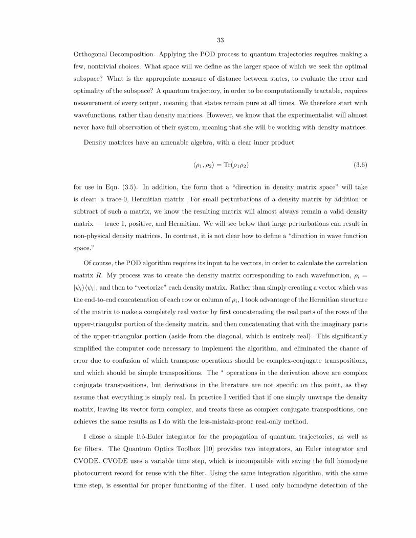
31

Chapter 3

Linear Models from ProperOrthogonal Decomposition

Proper Orthogonal Decomposition (POD), alternatively known as Principal Component Analysis

or the Karhunen-Loeve decomposition, is a model-reduction technique which generates the optimal

linear subspace of dimension D for a given set of higher-dimensional data. That is, if the data

are contained within an attractor, the POD process can produce the affine linear space that best

approximates the space containing that attractor. In this Chapter, I give a short derivation of the

POD algorithm, then show the results from applying it to two different bistable atom-cavity regimes.

For each regime, I show the performance of filters based on these POD results.

3.1 Background

The Proper Orthogonal Decomposition (POD) process has been derived in a variety of fields, which

has resulted in it having several names. In fluid dynamics, it is known as the Karhunen-Loeve

decomposition, and has its origins in the work of Lumley [28]. The method itself had its origins in

Pearson [29] and again in Hotelling [30].

The derivation which follows is based on those presented by Lall et al. [31] and Zhang and Zha

[32]. We start with an empirical set of data — an unordered collection of N points x(i) in Rm. In the

cases to be examined below, these will be vectorized forms of the density matrix ρ. We would like to

build the optimal d-dimensional affine subspace of Rm, which will be isomorphic to R

d. Zhang and

Zha take the approach of building the optimal map from the lower dimensional space to the higher,

while Lall et al. choose to find the optimal projector from the larger space to the smaller. Here I

choose the latter path, because it is more consistent with our goal of projecting the dynamics into

the lower-dimensional space.

We would like to find the optimal projection matrix, Q ∈ Rm×m, from R

m to a d-dimensional

subspace of Rm. We define the optimal Q as that which minimizes the total squared perpendicular

32

distance of the original set of points from the d-dimensional plane:

E(Q) =

N∑

i=1

‖x(i) − Qx(i)‖2. (3.1)

We wish to find the optimal affine subspace, which must go through the mean of the data, so

we subtract the mean of all the x(i)s, x, from each point before proceeding. We next construct the

correlation matrix

R =

N∑

i=1

(x(i) − x)(x(i) − x)∗, (3.2)

and calculate its eigenvalues, ordered λ1 ≥ λ2 ≥ · · ·λm. It is then a standard result that

minQ

E(Q) =

m∑

l=m−d+1

λl. (3.3)

The magnitude of each eigenvalue measures the relative contribution of the direction corresponding

to the paired eigenvector to the data distribution as a whole. By cutting off the space at d dimensions,

we measure the error, E, by summing the eigenvalues corresponding to the directions we have chosen

to discard.

Turning now to constructing the projector into this optimal subspace, we make use of the or-

thonormal eigenvectors φ1, φ2, . . . φd corresponding to the largest eigenvalues. The approximate x(i)

to x(i) is given by

x(i) =

d∑

j=1

aijφj + x (3.4)

where

aij =⟨

x(i) − x, φj

⟩

. (3.5)

Now denote by P the d × m matrix whose rows are φ1, φ2, . . . φd. Then the approximant to x is

P ∗P (x− x)+ x, and y = P (x− x) are the new coordinates for x in the new, d-dimensional subspace.

In this derivation, we have assumed an a priori known, fixed, d, but in practice one constructs R,

and then examines its eigenvalues, choosing d such that the error (3.3) is below whatever threshold

one decides.

3.2 Proper Orthogonal Decomposition of quantum trajecto-

ries

In attempting to better understand, and approximate, open quantum systems, we might like to

find lower-dimensional spaces in which the dynamics are confined, and for this we turn to Proper

33

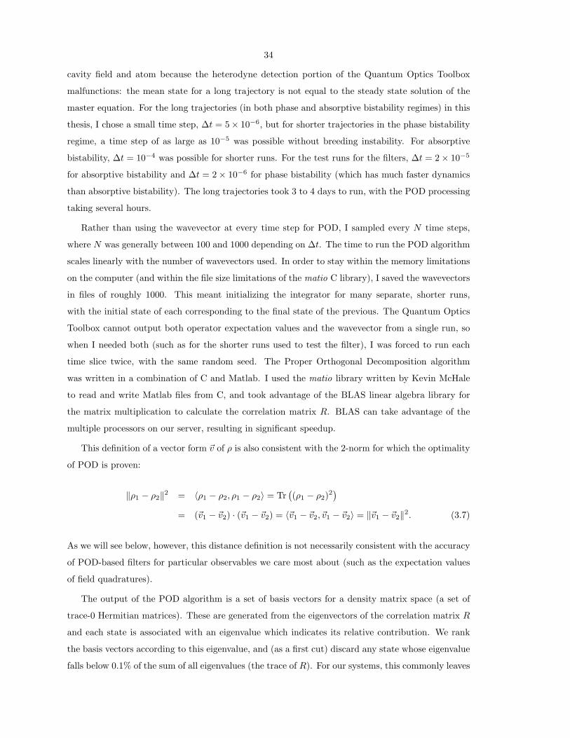
Orthogonal Decomposition. Applying the POD process to quantum trajectories requires making a

few, nontrivial choices. What space will we define as the larger space of which we seek the optimal

subspace? What is the appropriate measure of distance between states, to evaluate the error and

optimality of the subspace? A quantum trajectory, in order to be computationally tractable, requires

measurement of every output, meaning that states remain pure at all times. We therefore start with

wavefunctions, rather than density matrices. However, we know that the experimentalist will almost

never have full observation of their system, meaning that she will be working with density matrices.

Density matrices have an amenable algebra, with a clear inner product

〈ρ1, ρ2〉 = Tr(ρ1ρ2) (3.6)

for use in Eqn. (3.5). In addition, the form that a “direction in density matrix space” will take

is clear: a trace-0, Hermitian matrix. For small perturbations of a density matrix by addition or

subtract of such a matrix, we know the resulting matrix will almost always remain a valid density

matrix — trace 1, positive, and Hermitian. We will see below that large perturbations can result in

non-physical density matrices. In contrast, it is not clear how to define a “direction in wave function

space.”

Of course, the POD algorithm requires its input to be vectors, in order to calculate the correlation

matrix R. My process was to create the density matrix corresponding to each wavefunction, ρi =

|ψi〉〈ψi|, and then to “vectorize” each density matrix. Rather than simply creating a vector which was

the end-to-end concatenation of each row or column of ρi, I took advantage of the Hermitian structure

of the matrix to make a completely real vector by first concatenating the real parts of the rows of the

upper-triangular portion of the density matrix, and then concatenating that with the imaginary parts

of the upper-triangular portion (aside from the diagonal, which is entirely real). This significantly

simplified the computer code necessary to implement the algorithm, and eliminated the chance of

error due to confusion of which transpose operations should be complex-conjugate transpositions,

and which should be simple transpositions. The ∗ operations in the derivation above are complex

conjugate transpositions, but derivations in the literature are not specific on this point, as they

assume that everything is simply real. In practice I verified that if one simply unwraps the density

matrix, leaving its vector form complex, and treats these as complex-conjugate transpositions, one

achieves the same results as I do with the less-mistake-prone real-only method.

I chose a simple Ito-Euler integrator for the propagation of quantum trajectories, as well as

for filters. The Quantum Optics Toolbox [10] provides two integrators, an Euler integrator and

CVODE. CVODE uses a variable time step, which is incompatible with saving the full homodyne

photocurrent record for reuse with the filter. Using the same integration algorithm, with the same

time step, is essential for proper functioning of the filter. I used only homodyne detection of the

34

cavity field and atom because the heterodyne detection portion of the Quantum Optics Toolbox

malfunctions: the mean state for a long trajectory is not equal to the steady state solution of the

master equation. For the long trajectories (in both phase and absorptive bistability regimes) in this

thesis, I chose a small time step, ∆t = 5× 10−6, but for shorter trajectories in the phase bistability

regime, a time step of as large as 10−5 was possible without breeding instability. For absorptive

bistability, ∆t = 10−4 was possible for shorter runs. For the test runs for the filters, ∆t = 2 × 10−5

for absorptive bistability and ∆t = 2 × 10−6 for phase bistability (which has much faster dynamics

than absorptive bistability). The long trajectories took 3 to 4 days to run, with the POD processing

taking several hours.

Rather than using the wavevector at every time step for POD, I sampled every N time steps,

where N was generally between 100 and 1000 depending on ∆t. The time to run the POD algorithm

scales linearly with the number of wavevectors used. In order to stay within the memory limitations

on the computer (and within the file size limitations of the matio C library), I saved the wavevectors

in files of roughly 1000. This meant initializing the integrator for many separate, shorter runs,

with the initial state of each corresponding to the final state of the previous. The Quantum Optics

Toolbox cannot output both operator expectation values and the wavevector from a single run, so

when I needed both (such as for the shorter runs used to test the filter), I was forced to run each

time slice twice, with the same random seed. The Proper Orthogonal Decomposition algorithm

was written in a combination of C and Matlab. I used the matio library written by Kevin McHale

to read and write Matlab files from C, and took advantage of the BLAS linear algebra library for

the matrix multiplication to calculate the correlation matrix R. BLAS can take advantage of the

multiple processors on our server, resulting in significant speedup.

This definition of a vector form ~v of ρ is also consistent with the 2-norm for which the optimality

of POD is proven:

‖ρ1 − ρ2‖2 = 〈ρ1 − ρ2, ρ1 − ρ2〉 = Tr(

(ρ1 − ρ2)2)

= (~v1 − ~v2) · (~v1 − ~v2) = 〈~v1 − ~v2, ~v1 − ~v2〉 = ‖~v1 − ~v2‖2. (3.7)

As we will see below, however, this distance definition is not necessarily consistent with the accuracy

of POD-based filters for particular observables we care most about (such as the expectation values

of field quadratures).

The output of the POD algorithm is a set of basis vectors for a density matrix space (a set of

trace-0 Hermitian matrices). These are generated from the eigenvectors of the correlation matrix R

and each state is associated with an eigenvalue which indicates its relative contribution. We rank

the basis vectors according to this eigenvalue, and (as a first cut) discard any state whose eigenvalue

falls below 0.1% of the sum of all eigenvalues (the trace of R). For our systems, this commonly leaves

35

between 10 and 50 eigenstates. Further cuts are always done in the order of increasing eigenvalue,

but may be based on the performance of the projected filter or a more subjective sense that the states

below a certain eigenvalue look more like noise than states which would significantly contribute to

a more accurate approximation.

Proper Orthogonal Decomposition (and various modifications thereof) can produce subspaces

which look like they include the relevant parts of the system dynamics. However, we must evaluate

them quantitatively. To do this, we project the system dynamics onto several of these subspaces,

using the method derived in Section (2.2), and compare the dynamics indicated by the filter with the

trajectory dynamics. In this chapter, I use only the normalized dynamical system; the un-normalized

system performs slightly less well, and feels slightly less rigorous, due to the necessary renormalization

at each time step. The un-normalized projected system also requires re-orthogonalizing the set of

states to be used, because the mean state is not orthogonal to the other POD basis states. This in

turn means that we lose some of the clarity from the ordering of the states by eigenvalue.

3.3 Phase bistability

The density matrix (and associated Q function) for a phase bistable cavity QED system has a simple

structure — roughly, it is the superposition of two compact states with equal amplitude but opposite

phase. Q function dynamics consists largely of a compact, roughly Gaussian, peak located at one

stable point or the other, or in transition along the path between them. This superficially linear

form gives us hope that the linear approximations made in the POD algorithm will not significantly

impair performance, and a relatively low-dimensional, high fidelity approximation will be possible.

In fact, this hope is largely fulfilled.

Our canonical phase bistable system, used for all of the examples in this thesis, has the following

parameter values: Θ = 0, ∆ = 0, κ = 4, γ = 2, g0 = 12 and E = 23.57. This corresponds to the

set of parameters also used in [11]. (Van Handel and Mabuchi use superficially different values, but

the ratios determine behavior; in effect I have simply scaled time differently). Expectation values

from an excerpt of an example trajectory are shown in Figures 3.3 and 3.4. The trajectory I used

to generate the basis states for the subspace onto which we hope to project dynamics was run for

5000 units of time, with a time-step of ∆t = 5 × 10−6.

The Q functions of the mean (steady state) and the first 11 eigenstates (potential basis vectors)

are shown in Figure 3.1. While Q functions for valid quantum states are by definition always

positive, the potential basis vectors have Q functions which can swing wildly negative. Recall that

these are not quantum states, but rather directions; the Q function is simply an aid to the eye and

understanding. A projected state consists of some linear combination of these basis vectors, added

to the mean state; the Q functions roughly “add” as well. For example, a state which is composed

36

by adding the leading eigenstate to the mean would add probability density to one of the two states,

while removing it from the other; in effect this first basis direction alone can capture the switching

behavior (as we will see in the filter performance evaluation below). Notice that this switching

behavior will generally result in rather large components in the direction of this leading eigenstate,

threatening the “small perturbation” limit in the linearizing POD process. I get away with this

stretching of the POD approximations, I believe, only because the phase bistable system is so simple

and symmetric; if the two states were asymmetric I would be forced to undertake the additional

complicating procedures I discuss below in the context of (asymmetric) absorptive bistability.

The subsequent states capture behavior within the switching region, or dynamics within one

state. The transition basis states take a form similar to sinusoidal peaks and valleys between the

two stable states, and we may think of them as the basis states for a Fourier decomposition of a

single peak traveling between the two states (behavior which the leading eigenstate cannot capture).

Eigenstates beyond the 12th become hard to understand, and their eigenvalues are all less than 0.5%

of the sum of all eigenvalues. If we keep the first 12 states, we have kept eigenvalues which sum

to 97.3% of the total of all eigenvalues. See Figure 3.2 for a plot of the 60 largest eigenvalues in

descending order.

3.3.1 Projection filters

In order to evaluate the performance of the POD-produced approximations, I ran a long, high-

resolution (small time-step), quantum trajectory, separate from the trajectory on which the POD

algorithm was run. The homodyne photocurrent from the phase quadrature measurement, as well

as the expectation values of many system operators, were recorded for comparison with the filter.

In addition, I kept 5000 sampled wavefunctions in order to evaluate the fidelity of the approximate

states using a variety of measures of quantum fidelity.

Figure 3.3 shows the expectation values for the phase quadrature of the cavity field, 〈y〉, from

a short excerpt of this trajectory, with the quantum trajectory in blue. Comparable traces of 〈y〉from filters produced by projecting onto a subspace with 1, 4, 8, and 12 basis states are shown in

green, red, cyan, and magenta. Examining these in order, we first see that even a single-dimensional

subspace captures the switching behavior of the system (and it does it while stretching the definition

of a “small” difference from the mean implicit in our linearized system). However, the 1-D subspace

does not capture the transition dynamics between the two states — on the second transition in

Figure 3.3, it is closer to a square wave than the decaying exponential of the full trajectory. Adding

three basis states, which include some information about states between the two stable ones (see

Figure 3.1), allow this transition to exhibit some “decay,” while with 8 or 12 states the approximate

system can follow the exponential more closely.

Looking now at the first transition, the instabilities of the filter system become apparent. A

37

2 4 6 8-4

-2

0

2

4

2 4 6 8-4

-2

0

2

4

2 4 6 8-4

-2

0

2

4

2 4 6 8-4

-2

0

2

4

2 4 6 8-4

-2

0

2

4

2 4 6 8-4

-2

0

2

4

2 4 6 8-4

-2

0

2

4

2 4 6 8-4

-2

0

2

4

2 4 6 8-4

-2

0

2

4

2 4 6 8-4

-2

0

2

4

2 4 6 8-4

-2

0

2

4

Eigenstate 1

2 4 6 8-4

-2

0

2

4MEAN Eigenstate 2

Eigenstate 4

Eigenstate 3

Eigenstate 10 Eigenstate 11

Eigenstate 6

Eigenstate 9

Eigenstate 5

Eigenstate 8

Eigenstate 7

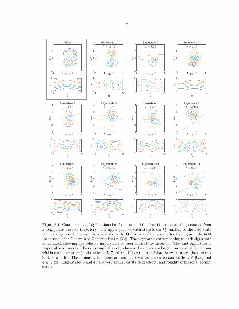
Figure 3.1: Contour plots of Q functions for the mean and the first 11 orthonormal eigenstates froma long phase bistable trajectory. The upper plot for each state is the Q function of the field stateafter tracing over the atom; the lower plot is the Q function of the atom after tracing over the field(produced using Generalized Coherent States [33]). The eigenvalue corresponding to each eigenstateis included, showing the relative importance of each basis state/direction. The first eigenstate isresponsible for most of the switching behavior, whereas the others are largely responsible for motionwithin each eigenstate (basis states 2, 5, 7, 10 and 11) or the transitions between states (basis states3, 4, 8, and 9). The atomic Q functions are parametrized on a sphere spanned by θ ∈ [0, π] andφ ∈ [0, 2π]. Eigenstates 3 and 4 have very similar cavity field effects, and roughly orthogonal atomicstates.

38

10 20 30 40 50

-5

-4

-3

-2

-1

0

Figure 3.2: Eigenvalues of the correlation matrix R for the canonical phase bistable case, shown asthe logarithm of the fraction of total eigenvalues, for the 60 eigenstates with largest eigenvalues.

segment of (noisy) photocurrent here apparently contains relatively little accurate information about

the state, the state is only very poorly approximated by the limited subspaces in these 12-or-fewer

dimensional approximations, or the photocurrent excites the use of basis states which are not helpful

for stability. Similar patches of instability occur with some regularity, and are worst with 12 basis

states. In these areas, the filtered state is no longer a valid quantum state (with a positive semi-

definite density matrix). Not surprisingly, the fidelity measured between the wavefunction from the

quantum trajectory and the projected filter is quite poor in these areas.

I used two fidelity measures to evaluate the performance of this filter: Probability of Error

and the Bhattacharyya Coefficient. See Fuchs and van de Graaf [34] for a derivation of these two

coefficients, as well as the Kolmogorov Distance (which is intimately related the Probability of Error

and doesn’t contain any more information). The Probability of Error is defined as

PE(ρ0, ρ1) =1

2− 1

4

N∑

j=1

|λj |, (3.8)

where λj are the eigenvalues of (ρ0 −ρ1). This value should vary between 0 (two states are perfectly

distinguishable) and 1/2 (perfectly indistinguishable) as long as ρ0 and ρ1 are valid density matrices.

39

0 1 2 3 4 5 6 7 8

-2

-1

0

1

2

3

4

5

6

7

8

Figure 3.3: A short excerpt from a single phase-bistable quantum trajectory, showing the expectationvalue of the phase quadrature of the cavity field, 〈y〉, and the trajectories of three filters using thesame homodyne detection photocurrent. The trajectory is in blue, and the projected filters using 1,4, 8, and 12 basis states are shown in green, red, cyan, and magenta, respectively. The filters with 8and 12 basis states are somewhat less stable (witness the first and fourth transitions here), but givea closer approximation during the “quiescent” times between transitions, and fit the exponentialdecay shape of the second transition better than the 1 or 4 basis-state approximations. Projectingonto even a one-dimensional subspace, however, successfully captures the switching behavior of thesystem.

0 1 2 3 4 5 6 7 8-3

-2

-1

0

1

2

3

(a)

0 1 2 3 4 5 6 7 8-3

-2.5

-2

-1.5

-1

-0.5

0

0.5

1

1.5

2

(b)

0 1 2 3 4 5 6 7 8-2

-1.5

-1

-0.5

0

0.5

1

1.5

2

(c)

Figure 3.4: Trajectories of the three simple atomic Hermitian observables for the same time span asFigure 3.3. (a) σx, (b) σy, and (c) σz. For each observable, the red trace is the quantum trajectory;the blue trace is the filter with 12 basis states (the same filter as shown in magenta in Figure 3.3).

40

The Bhattacharyya Coefficient is defined as

B(ρ0, ρ1) = Tr√√

ρ0ρ1√

ρ0. (3.9)

Its value varies between 0 (orthogonal states) and 1 (identical states).

The calculated values of these two fidelity measures over the course of an extended filtering

simulation offer some surprises, which indicate both the failures of the filter, and differences between

these two measures. The average Probability of Error decreases as we include more states in our

basis, from 0.2065 with one basis state, to 0.2059 with 4, 0.1057 with 8 and -0.0708 with 12. What

is happening is that the periods of instability are dominating the average. In these areas, the

approximate state is not a valid quantum state, and the value of the “probability” can fall below

zero. However, if we examine just the quiescent periods between state transitions and unstable

patches, the Probability of Error is almost identical for the four filters.

The Bhattacharyya Coefficient (BC) behaves somewhat differently. In particular, when the filter

state becomes unphysical, the BC becomes imaginary, rather than negative (I use only the real

part of the BC, as the mean of the imaginary parts is very close to zero). This allows the average

value over a filtering run to stay almost constant with the size of the basis state, because the 12-

dimensional basis does provide for a slightly higher BC than the 8 in the “normal” periods, which

in turn has a higher BC than the 4- and 1-state filters. The unstable zones have a BC of zero, so the

increased instability from added basis states results in a falling average. The 1 state BC is 0.4364,

4 state BC is 0.4485, 8 state is 0.4463, and 12 state is 0.4355.

Proper Orthogonal Decomposition appears to work quite well to define a subspace in which the

phase bistable dynamics take place. The basis states (in Figure 3.1) capture both stable states,

and allow for approximations of both the dynamics within each state and the transitions between.

When stable, the projected filter can do a good job of matching the behavior of 〈y〉 and 〈σy〉; other

observables fluctuate quickly, while the filter approximates their mean. The occasional instability of

the filter, however, raises doubts as to whether POD is a robust solution.

3.4 Absorptive bistability

Absorptive bistability occurs as part of a much more complicated system than phase bistability. In

particular, the upper “state” is extended for our set of parameters (very different from the close-

to-minimum-uncertainty states in phase bistability). Complicating the performance of the Proper

Orthogonal Decomposition algorithm, the system can be significantly asymmetric between the upper

and lower states, depending on the driving field strength (phase bistability is structurally exactly

symmetric). I have chosen a driving field for the examples in this thesis at which the fraction of time

41

Eigenstate 1MEAN Eigenstate 2

Eigenstate 4

Eigenstate 3

Eigenstate 6Eigenstate 5 Eigenstate 7

-5

0

5

-2 0 2 4 6 8-5

0

5

-2 0 2 4 6 8-5

0

5

-2 0 2 4 6 8-5

0

5

-2 0 2 4 6 8

-5

0

5

-2 0 2 4 6 8-5

0

5

-2 0 2 4 6 8-5

0

5

-2 0 2 4 6 8-5

0

5

-2 0 2 4 6 8

Figure 3.5: The mean and leading 7 eigenstates from the Proper Orthogonal Decomposition al-gorithm applied to a long absorptive bistable trajectory. The first eigenstate allows the filter toremove almost all traces of the lower state, while the remaining eigenstates finish that cancellationand allow for dynamics within the upper state. No combination of these states, however, allows forthe cancellation of the full upper state in order to accurately approximate the lower stable state.The model parameters are Θ = 0, ∆ = 0, κ = 0.1, γ = 2, g0 =

√2, and E = 0.56, and the simulation

was run for tfinal = 5000 (with time scaled by γ/2).

spent in each state is roughly equal; however, this may not be the experimentalist’s preferred (or

available) parameter value, resulting in lower POD performance unless the algorithm is extended,

as I will describe later in this subsection.

The parameters I have chosen to demonstrate the application of POD to an absorptively bistable

system are: Θ = 0, ∆ = 0, κ = 0.1, γ = 2, g0 =√

2, and E = 0.56. (This is clearly a “good cavity”

relative to our phase bistable system; we achieve similar cavity field amplitudes for almost 2 orders

of magnitude less driving field intensity.) Notice that this driving field strength is above the upper

semi-classical (Maxwell-Bloch) bifurcation point (E ≈ 0.553); that is, the semi-classical system has

only one stable point at this driving field value. These are similar to the parameters chosen by [22],

except I have chosen a slightly lower driving field in order to get closer to an even balance between

the lower and higher amplitude states.

Simply applying the POD algorithm to a long (tfinal = 5000) trajectory (with homodyne mea-

surement of field amplitude quadrature) results in the set of states shown in 3.5. Note that the

42

0 100 200 300 400 500 600 700 800 900 10000

0.5

1

1.5

2

2.5

3

3.5

4

4.5

5

Figure 3.6: Comparison in the absorptive bistability regime of simple POD filter with exact quantumtrajectory. The blue trace is the expected value of the amplitude quadrature for a POD filter witha 7-dimensional linear subspace; the red trace is from the quantum trajectory. The eigenvaluescorresponding to these leading 7 eigenstates sum to 99.85% of the sum of all eigenvalues; the largesteigenvalue left out is less that 0.08% of the total. Amplitude quadrature homodyne measurement;params.

states beyond the first generally relate to directions in the upper state, and none of these first 8

basis vectors allow for dynamics or fluctuations within the lower state. We know from observing

the trajectory that what dynamics there are within the lower state are smaller in amplitude than

those within the upper state. The first eigenstate is generally responsible for the switching behavior:

subtract this from the mean to move towards the upper state alone, and add it to move toward the

lower state alone. Note, however, that the shape of the upper portion of this basis state does not

match the shape of the upper portion of the mean, so that adding this state alone will not put us

exactly in the lower state. The shapes match much more clearly for the lower state, so if we subtract

the correct multiple of this basis state from the mean we can almost exactly cancel the lower state.

The second and higher basis states allow for some fluctuations within the upper state.

This asymmetry between the lower and upper states results in significantly impaired performance

as a filter. Using 7 eigenstates to make the basis of the subspace into which we project the dynamics,

we plot 〈x〉 from the projected dynamics in Figure 3.6. The eigenvalues corresponding to these

leading 7 eigenstates sum to 99.85% of the sum of all eigenvalues; the largest eigenvalue eliminated

43

is less that 0.08% of the total. The filter tries to match the field amplitude of the lower state, but

simply cannot, because the subspace does not include a good approximation to the lower state. The

mismatch in shapes results in a minimum achievable 〈x〉 which is above that of the lower state.

The filter does relatively much better with the upper state, although it cannot capture all of the

volatility. It is able to track some of the fluctuations down from the upper state, but cannot go

higher than a fixed value. It is also unable to track the volatility in 〈y〉 within the upper state (not

shown).

Needless to say, the fidelity of this filter is quite poor. The mean Probability of Error is negative

(−0.008), thanks to long periods (in the lower state) in which the filter state is not a valid density

matrix (negative eigenvalues, and the Q function not positive everywhere). The Probability of Error

measure is positive during the times when the system is in the upper state, averaging around 0.02,

with a maximum of 0.155. The mean Bhattacharyya Coefficient is 0.185, with an average of about

0.13 in the lower state, and 0.24 (but wildly varying between 0.012 and 0.6) in the upper state. The

resilience of the Bhattacharyya Coefficient to unphysical filter states makes it a somewhat preferred

measure.

Some trajectories randomly spend a larger fraction of their time in the lower state than the one

I used here, and these trajectories can exhibit the opposite problem as a filter: they capture the

lower state and its dynamics well, but badly miss the upper state. In order to address this problem,

I tried two different strategies: weighting the sum used to calculate distances in the density matrix

space, and dividing the data into three “zones”: lower, transition, and upper, and executing POD

separately in each zone.

3.4.1 Weighted POD

The observables we tend to care most about in evaluating the accuracy of our model reduction are the

5 observables whose dynamics can be approximated by the Maxwell-Bloch equations: 〈x〉, 〈y〉, 〈σx〉,〈σy〉, and 〈σz〉. In matrix form (to act on density matrices), the nonzero terms for these observables

lie on the diagonal or immediate off-diagonal. (For a tensor product system like an two-level-atom

and cavity system, let us define the “diagonal” to be the diagonal of each quadrant.) The values

of these observables (calculated as Tr(Oρ) for each operator O), then, depend only on the diagonal

and immediate off-diagonal terms in the density matrix. Proper Orthogonal Decomposition, on the

other hand, treats every entry in the density matrix identically. POD produces the optimal subspace

provided that we share its definition of distance, which treats the real and imaginary parts of each

entry in a completely even-handed fashion. The failure of POD to produce a single subspace which

includes both the upper and lower states can be partly attributed to this evenhandedness: dynamics

within the upper state win out over including an accurate approximation for the lower state.

To address this, I tested various re-definitions of distance by weighting the terms of the density

44

matrix. To do this, I defined the distance from the diagonal nd to be the the absolute value of the

difference between i and j labels for each entry in the matrix (modulo half the matrix size to allow

for the tensor product structure). I then divided each entry by nXd where X = 0.5, 1, or 2. This

process treats the diagonal differently from the immediate off-diagonal, so I also used a weighting

scheme which measured distance from the immediate off-diagonal, so that the weighting would follow

the pattern (B) 1, 1, 1/2, 1/3, 1/4, . . . instead of (A) 1, 1/2, 1/3, 1/4, . . . as we proceed away from

the diagonal. None of these six weighting schemes has any appreciable effect on the balance between

the upper and lower states, relative to basic POD (X = 0). All produce basis states similar to those

shown in Figure 3.5, with only dynamics of the upper state represented, and fail as filters because

they cannot come close to approximating the lower state.

There is another inequity between the distribution of density matrix entries and the distribution

of expectation values: the density of Fock states scales like the square of the amplitude of a coherent

state, so that a state further from the vacuum has large entries in many more locations in the

density matrix than one close to the vacuum. Imagine two pairs of states, one pair close to the

vacuum, and one with 〈x〉 ≈ 4. The distance within each pair, when measured in the way we defined

for Proper Orthogonal Decomposition, is the same. However, the pair close to the vacuum will

have substantially different expectation values, while the higher amplitude pair might be almost

indistinguishable by that measure. What skews POD is the reverse of this: small fluctuations

in expectation values at high amplitude look like large distances in the POD metric, while small

fluctuations near the vacuum are small in this metric. This is compounded by the behavior in the

absorptive bistability regime, which has larger fluctuations in the upper state, and the POD process

outputs states which focus on the upper state and do a very poor job in the lower.

To counteract this, I tried a weighting scheme which weights the vacuum state highest, and decays

away from there. We know a priori that the scaling should go like the square root of the Fock state

in order for the distance to be independent of the coherent amplitude. Applied to the POD process,

this weighting also has no appreciable effect on the fundamental problem: the lower state is not

accurately approximated by combinations of the dominant eigenstates. This makes sense because at

the same time that this weighting reduces the effective distance between density matrices within the

upper state, it also undercounts the remnants of the upper state which are left behind when using

the leading eigenstate (see Figure 3.5) to attempt to approximate the lower state. For weighted

POD to improve on the unweighted process, we would need a weighting scheme which somehow

simultaneously counts and discounts the higher-field-amplitude portions of the density matrix. One

possibility, unexplored in this thesis, would be to move the origin for the POD analysis to the space

between the lower and upper “states,” so that they both have similar amplitude and take up similar

“space” within the density matrix. They will still be asymmetric, however, in both shape and the

time the system spends in each (especially if the driving field is not selected for balance between

45

states). Fundamentally, Proper Orthogonal Decomposition with a single mean, and perturbations

around that mean, has difficultly handling dynamics around two separated, asymmetric states.

3.4.2 Zoned POD

Proper Orthogonal Decomposition implicitly makes “small perturbation” assumptions, which we

violate when we consider a system with multiple stable points, as the leading eigenstates end up with

quite large coefficients to push unto into one stable regime or another. In addition, the algorithm’s

emphasis on the dominant, most common states means that it tells us almost nothing about the

transitions between states when there are significant dynamics within states. The phase bistable

system considered in Section 3.3 is symmetric enough, and switches often enough, that the switching

dynamics and the transition periods are on a more level footing with fluctuations and dynamics

within each state. The absorptive bistability regime is not symmetric, and transitions are much

more rare. We can improve compliance with assumptions, capture some transition behavior, and

re-balance asymmetry by diving the data into zones surrounding each stable point, and in between

them.

For the driving field strength, cavity damping rate, and other parameters which define our

standard absorptive bistability regime, the lower state has a mean cavity field amplitude of about

0.5, and the upper state (while broader) has a mean of about 3.25. The fluctuations around these two

states rarely cross into the range of 1.5 to 2.5 unless the system is actually in transition between the

two stable regions. Therefore, I cut the data into three sets: “lower” for any point in the trajectory

which has 〈x〉 < 1.5, “upper” for points with 〈x〉 > 2.5, and “transition” for points in between. (I

include a short segment on either side of the exact transition zone to associate behavior leading to

or out of transitions with them, rather than with the lower or upper zones.) Note that the constant

measurement and decay of the system helps keep the field states compact. They are almost always

roughly Gaussian (with a Q function width similar to the width of a coherent state), so we can use

〈x〉 as a proxy for the full distribution.

Once we have divided the data into three subsets, we have two options for defining the mean state

for the POD algorithm: we could continue to use the overall mean, or find the mean of each zone.

In the former case, the leading eigenstate will be the direction from the overall mean to some part of

that zone, and subsequent basis states provide a direction within the zone. The latter case creates

the transition direction directly, without use of POD, simply by subtracting the zone’s mean from

the overall mean. All the POD basis states are then directions away from that local mean. I have

tried both definitions, but selected the latter because it is most consistent with the small-coefficient

assumptions built in to POD and because the means will be independent of small asymmetries which

might otherwise throw the leading eigenstate “off balance.” This is particularly a concern for the

transition zone, where the relatively small number of transitions means that if more transitions take

46

place with 〈y〉 > 0 than 〈y〉 < 0, the “one mean” algorithm would likely select the leading eigenstate

to reflect just the 〈y〉 > 0 transitions, biasing all the subsequent eigenstates as well.

The output of three separate POD processes (one for each zone) is three sets of Hermitian

matrices, from which we will build our subspace. (Implementation of the algorithm tends to produce

matrices which are almost but not exactly Hermitian, due to numerical errors; I added a simple step

which tweaks them to be exactly Hermitian.) There are four matrices with trace 1 (valid density

matrices): the overall mean and the mean of each zone. I turn the zone means into trace-0 (direction)

matrices by subtracting the overall mean. The remaining matrices are already directions in density

matrix space, but they are not all orthonormal. The directions within each zone are orthogonal

(although not orthogonal to the newly-created “mean direction” for that zone), but they are not

orthogonal between zones. We therefore run the set of all trace-0 direction matrices (including

the means) through a simple inner-product based orthonormaliztion process. Because they are all

Hermitian, their inner products are all real, and their linear combinations with real coefficients

produce new, orthonormal, direction matrices which remain Hermitian. The linear combinations

which result from filtering will therefore be valid density matrices as long as they remain positive

definite.

Figures 3.7 and 3.8 show the leading states from two different trajectories in the absorptive

bistability regime. Figure 3.7 results from a trajectory in which the cavity field was measured in the

amplitude quadrature; Figure 3.8 was measured in the phase quadrature. (Note that both show their

set of states before they have been orthonormalized.) Because the steady states and behavior of a

quantum system do not depend on the measurement, it’s not surprising that these two sets of states

are quite similar. They do provide an opportunity to examine the some of the kinds of differences

which result from different trajectories. For example, the lower zone eigenstates are arranged at

different angles, indicating that the noise in the lower state scattered more in one axis than another

during the trajectory.

In both cases, the transition zone is biased towards 〈y〉 > 0 behavior in its leading eigenstates.

Each of these trajectories include only a dozen or so transitions, meaning that the statistics are

quite poor. A much longer trajectory (which would require a more patient researcher and/or a

more powerful computer) ought to have more balanced eigenstates in the transition zone. These

higher-quality eigenstates might allow us to see whether transitions favor particular paths in phase

space. In particular, the semi-classical Maxwell-Bloch equations have an unstable point between the

two stable equilibria (see Figure 1.2), and these transition states might reveal whether the quantum

system avoids the 〈y〉 = 0, 〈x〉 ≈ 2 area, or not. I cannot draw conclusions on this point from the

limited trajectories I have been able to analyze.

To test the performance of these POD subspaces, I ran them as a filter on the same homodyne

photocurrent as in Figure 3.6 and the surrounding discussion. A disadvantage of the zoned approach

47

Lower MeanMEAN Low State 1

Low State 3

Low State 2

Upper State 2 Upper State 3

Transition State 1

Upper State 1

Transition Mean

Upper Mean

Transition State 2

-5

0

5

-2 0 2 4 6 8-5

0

5

-2 0 2 4 6 8-5

0

5

-2 0 2 4 6 8-5

0

5

-2 0 2 4 6 8

-5

0

5

-2 0 2 4 6 8-5

0

5

-2 0 2 4 6 8-5

0

5

-2 0 2 4 6 8-5

0

5

-2 0 2 4 6 8

-5

0

5

-2 0 2 4 6 8-5

0

5

-2 0 2 4 6 8-5

0

5

-2 0 2 4 6 8-5

0

5

-2 0 2 4 6 8

Figure 3.7: Contour plots of Q functions for states and basis vectors from “zoned” Proper Orthog-onal Decomposition of absorptive bistability regime, with homodyne measurement of cavity fieldamplitude quadrature. The upper plot for each state is the Q function of the field state after tracingover the atom; the lower plot is the Q function of the atom after tracing over the field (producedusing Generalized Coherent States [33]). Four states are generated separately from POD: the overallmeans state and the mean states in each of three zones. The leading 2 or 3 eigenstates from eachzone are shown, along with the eigenvalue corresponding to each, showing the relative importanceof each basis state/direction. The atomic Q functions are parametrized on a sphere spanned byθ ∈ [0, π] and φ ∈ [0, 2π].

48

Lower MeanMEAN Low State 1

Low State 3

Low State 2

Upper State 2 Upper State 3

Transition State 1

Upper State 1

Transition Mean

Upper Mean

Transition State 2

-5

0

5

-2 0 2 4 6 8-5

0

5

-2 0 2 4 6 8-5

0

5

-2 0 2 4 6 8-5

0

5

-2 0 2 4 6 8

-5

0

5

-2 0 2 4 6 8-5

0

5

-2 0 2 4 6 8-5

0

5

-2 0 2 4 6 8-5

0

5

-2 0 2 4 6 8

-5

0

5

-2 0 2 4 6 8-5

0

5

-2 0 2 4 6 8-5

0

5

-2 0 2 4 6 8-5

0

5

-2 0 2 4 6 8

Figure 3.8: Contour plots of Q functions for states and basis vectors from “zoned” Proper OrthogonalDecomposition of absorptive bistability regime, with homodyne measurement of cavity field phase

quadrature. The upper plot for each state is the Q function of the field state after tracing overthe atom; the lower plot is the Q function of the atom after tracing over the field (produced usingGeneralized Coherent States [33]). Four states are generated separately from POD: the overall meansstate and the mean states in each of three zones. The leading 2 or 3 eigenstates from each zone areshown, along with the eigenvalue corresponding to each, showing the relative importance of eachbasis state/direction. The atomic Q functions are parametrized on a sphere spanned by θ ∈ [0, π]and φ ∈ [0, 2π].

49

0 100 200 300 400 500 600 700 800 900 10000

0.5

1

1.5

2

2.5

3

3.5

4

4.5

5

(a)

-4

-3

-2

-1

0

1

2

3

4

0 100 200 300 400 500 600 700 800 900 1000

(b)

Figure 3.9: Comparison in the absorptive bistability regime of a “zoned” POD filter with exactquantum trajectory. The blue trace is the expected value of the amplitude quadrature for a PODfilter with a 12-dimensional linear subspace; the red trace is from the quantum trajectory. Thesubspace is constructed from the mean states within each zone and the leading 3, 2, and 4 eigenstatesfrom the lower, transition, and upper zones, respectively. Filter constructed and run on a systemwith a homodyne measurement on the amplitude quadrature.

is that we need to include more basis states, because we need the leading few from each zone. As

an example, I chose to run the filter using a 12-dimensional subspace: the “lower mean” and the

leading 3 eigenstates from the lower zone, “transition mean” and leading 2 eigenstates from the

transition zone, and “upper mean” and 4 states from the upper zone. This means I am including

98.9% of the eigenvalue sum in the lower zone, 91.2% in the transition, and 98.3% in the upper zone,

with 12 dimensions to consider (instead of 7 as in the basic POD filter above). As expected, this

filter significantly outperforms the basic POD filter, helped immensely by its ability to successfully

approximate both the lower and upper states. Figure 3.9 demonstrates the ability of the amplitude

quadrature zoned filter to successfully capture the lower and upper states, as well as some of the

dynamics within each. The large fluctuations within the upper state still prove to be too much for

the “small amplitude” approximation built into the POD formulation.

The Probability of Error fidelity measure is somewhat better for the “zoned” POD than for the

basic algorithm: at least the mean is positive (0.0134). The mean in the lower state is approximately

0.005, and it is somewhat better (0.027) in the upper state away from the few points where the filter

becomes unphysical. The maximum Probability of Error for this data set was 0.09. The Bhat-

tacharyya Coefficient similarly shows slight, but notable, improvement using the “zoned” algorithm

relative to the basic POD process. The mean value of BC for this data set is 0.199 (compared to

0.185). The average in the lower state is about 0.17, and 0.22 in the upper state. Note that this

reflects the markedly better performance for the zoned algorithm in the lower state and slightly

worse performance in the upper state (perhaps due to the inclusion of only 4 eigenstates related to

dynamics within that zone, compared with 6 in the simple POD algorithm).

50

If we discard the results of POD entirely, and use only the mean states for each zone, we end

up with a reasonable filter, at least for amplitude quadrature behavior (it has no flexibility to

capture the phase quadrature or atomic behavior). This 3-dimensional filter underperforms the 12-

dimensional one, but might suffice for some applications. The mean Probability of Error is 0.0086

(with a mean of 0.0058 in the lower state, 0.0192 in the upper state, and a maximum of almost

0.08). The Bhattacharyya Coefficient is almost unchanged in this case for the lower state (where

internal dynamics play a smaller role, so discarding them has a smaller effect), with a mean of 0.17.

It performs less well in the upper state, as expected, with a mean of 0.215. The overall mean BC

for this non-POD filter is 0.195.

The filter for homodyne measurement of the phase quadrature, using the same distribution of

eigenstates as the amplitude quadrature, utterly fails as a reasonable filter. It behaves somewhat

reasonably in the lower state, but fails in the upper state. To see why, look at the variation of

the phase quadrature, 〈y〉, in Figure 3.9b, and compare it with the y-extent of the eigenstates in

Figure 3.8. A filter based on the homodyne photocurrent from a phase quadrature measurement will

attempt to match the observed value of the phase, but to do so given the eigenstates even from zoned

POD requires unphysical states from combinations with large coefficients. In turn, these unphysical

states do not do a good job of reproducing the other observables (like 〈x〉), and the fidelity of the

filter to the actual dynamics is negligible (and the filter tends to be very unstable). This is not only

a product of this “zoned” POD process: the same thing happens with basic, un-zoned POD, and

with zoned basis states calculated using only the single overall mean (rather than the means for each

zone).

3.5 Discussion

As we have seen in this chapter, Proper Orthogonal Decomposition is capable, when used with care

and extended when necessary, of producing low-dimensional linear models which capture some of the

dominant dynamics of quantum systems. Basic POD, applied to the phase bistable case, produced

filters that are usually highly accurate at capturing the broad dynamics of the system, and might

serve as reasonable filters for a control application. When extended into “zones,” POD also works

quite well for absorptive bistability, as long as the basis states used include close to the full range

for the variable being measured (the amplitude quadrature for our example).

POD is not a universal tool, however, and its limitations in both the phase and absorptive

bistability regimes illustrate broader issues that would arise should the tool be extended to other

systems. The first of these is the algorithm’s tendency to deliver spaces which include only the

type of dynamics in which the system spends the largest fraction of the time. In the phase bistable

case, the particular trajectory used as an example in this thesis spends slightly more time in one

51

state than the other. As a result, the basis set returned by POD favors some dynamics within this

slightly-favored state over dimensions that inform us about state transitions; this may not match

the order in which the experimentalist would emphasize these two behaviors.

This sensitivity to asymmetry is also at play in the absorptive bistability example, and is exac-

erbated by shape asymmetry between the upper and lower states. The definition of distance in the

density-matrix space, which is the most obvious choice for that metric, also contributes significantly

to this behavior. Even drastic interventions in this definition of distance, however, were unable to

qualitatively change the POD algorithm’s behavior (and resulting failing filter) to match the physical

system’s behavior.

At the root of concerns about asymmetry and distance is the fundamental limitation of Proper

Orthogonal Decomposition: it only captures directions away from a mean state, defines a linear

space, and fundamentally relates only to small perturbations away from the mean. Large dynamics

away from the mean and nonlinear underlying structures of the dynamics (such as multiple stable

states) all challenge POD in precisely this weak spot. Unfortunately, it is often precisely this behavior

which we wish to capture or control.

52