Linear Models 1 - rikhtehgaran.iut.ac.ir · The PDF versions of references are available in the...
14
Linear Models 1 Isfahan University of Technology Fall Semester, 2014 References: [1] G. A. F., Seber and A. J. Lee (2003). Linear Regression Analysis (2nd ed.). Hoboken, NJ: Wiley. [2] A. C. Rencher and G. B. Schaalje (2008). Linear Models in Statistics (2nd ed.). John Wiley & Sons, Inc. [3] R. B., Bapat (2000), Linear Algebra and Linear Models, (2 nd ed.). Springer-Verlag. [4] S. R., Searle (1971). Linear Models. New York: Wiley. The PDF versions of references are available in the link http://rikhtehgaran.iut.ac.ir/ Prerequisites: . Linear Algebra Basic Statistical Inference. Grading Policy: Assignments & Quizes: 3-5 points. Midterm Exam: 5-7 points . Final Exam: 10 points.
Transcript of Linear Models 1 - rikhtehgaran.iut.ac.ir · The PDF versions of references are available in the...
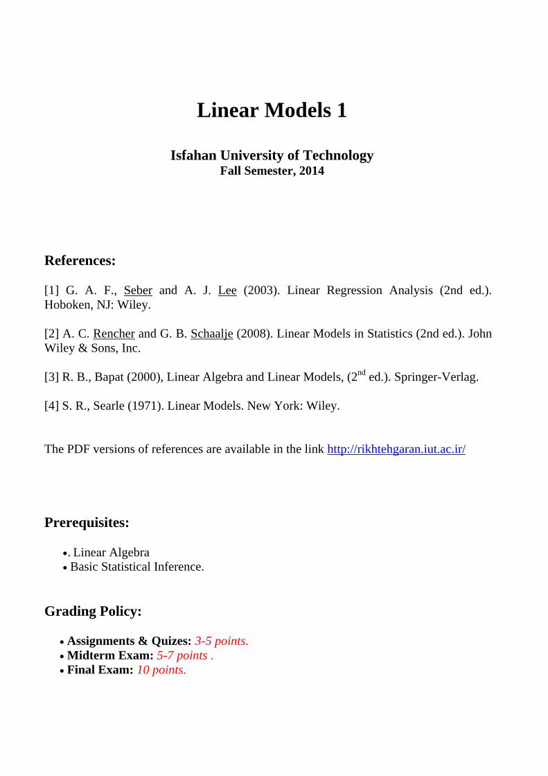
Linear Models 1
Isfahan University of Technology Fall Semester, 2014
References:
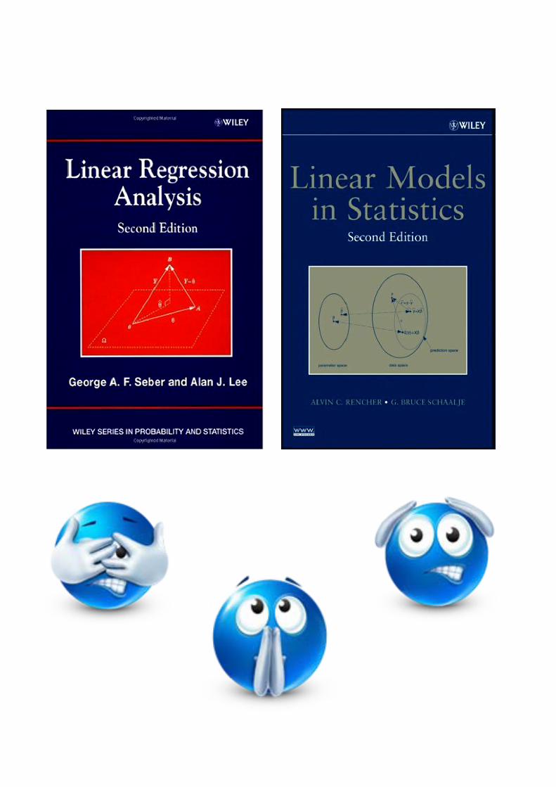
[1] G. A. F., Seber and A. J. Lee (2003). Linear Regression Analysis (2nd ed.). Hoboken, NJ: Wiley.
[2] A. C. Rencher and G. B. Schaalje (2008). Linear Models in Statistics (2nd ed.). John Wiley & Sons, Inc.
[3] R. B., Bapat (2000), Linear Algebra and Linear Models, (2nd ed.). Springer-Verlag.
[4] S. R., Searle (1971). Linear Models. New York: Wiley.
The PDF versions of references are available in the link http://rikhtehgaran.iut.ac.ir/
Prerequisites:
. Linear AlgebraBasic Statistical Inference.
Grading Policy:
Assignments & Quizes: 3-5 points.Midterm Exam: 5-7 points .Final Exam: 10 points.
R2
Accepted
R2
Accepted
R2
Rectangle
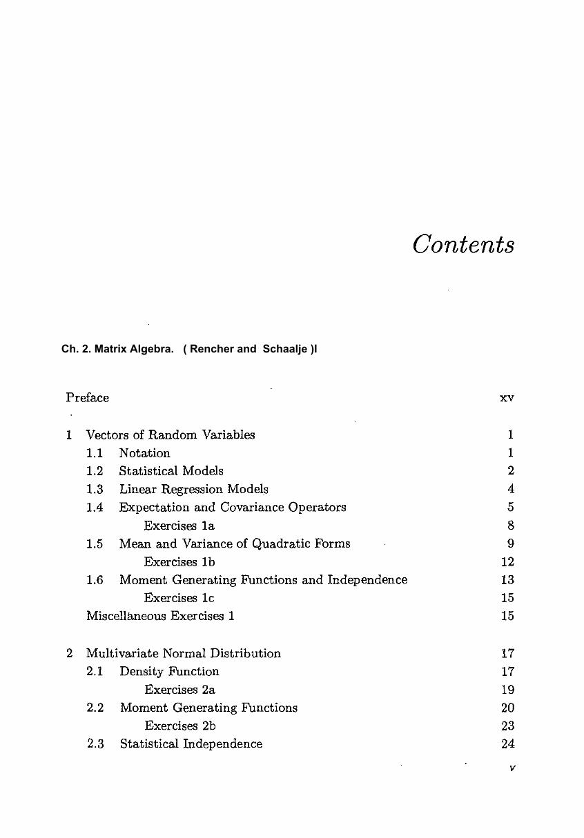
Contents
Preface xv
1 Vectors of Random Variables 1
1.1 Notation 1
1.2 Statistical Models 2
1.3 Linear Regression Models 4
1.4 Expectation and Covariance Operators 5 Exercises la 8
1.5 Mean and Variance of Quadratic Forms 9
Exercises 1 b 12
1.6 Moment Generating Functions and Independence 13 Exercises lc 15
Miscellaneous Exercises 1 15
2 Multivariate Normal Distribution 17 2.1 Density Function 17
Exercises 2a 19 2.2 Moment Generating Functions 20
Exercises 2b 23 2.3 Statistical Independence 24
v
Ch. 2. Matrix Algebra. ( Rencher and Schaalje )l
R2
Rectangle
R2
Rectangle
R2
Rectangle
R2
Pencil
R2
Line
R2
Line
R2
Line
R2
Text Box
y'Ay
VI CONTENTS
Exercises 2c 26
2.4 Distribution of Quadratic Forms 27
Exercises 2d 31
Miscellaneous Exercises 2 31
3 Linear Regression: Estimation and Distribution Theory 35
3.1 Least Squares Estimation 35
Exercises 3a 41
3.2 Properties of Least Squares Estimates 42
Exercises 3b 44
3.3 Unbiased Estimation of (72 44 Exercises 3c 47
3.4 Distribution Theory 47 Exercises 3d 49
3.5 Maximum Likelihood Estimation 49
3.6 Orthogonal Columns in the Regression Matrix 51 Exercises 3e 52
3.7 Introducing Further Explanatory Variables 54
3.7.1 General Theory 54 3.7.2 One Extra Variable 57
Exercises 3f 58
3.8 Estimation with Linear Restrictions 59 3.8.1 Method of Lagrange Multipliers 60
3.8.2 Method of Orthogonal Projections 61
Exercises 3g 62
3.9 Design Matrix of Less Than Full Rank 62 3.9.1 Least Squares Estimation 62
Exercises 3h 64
3.9.2 Estimable Functions 64 Exercises 3i 65
3.9.3 Introducing Further Explanatory Variables 65 3.9.4 Introducing Linear Restrictions 65
Exercises 3j 66 3.10 Generalized Least Squares 66
Exercises 3k 69
3.11 Centering and Scaling the Explanatory Variables 69 3.11.1 Centering 70 3.11.2 Scaling 71
R2
Rectangle
R2
Line
R2
Line
R2
Line
R2
Line
R2
Line
R2
Line
CONTENTS VII
Exercises 31 72 3.12 Bayesian Estimation 73
Exercises 3m 76 3.13 Robust Regression 77
3.13.1 M-Estimates 78 3.13.2 Estimates Based on Robust Location and Scale
Measures 3.13.3 Measuring Robustness 3.13.4 Other Robust Estimates
Exercises 3n Miscellaneous Exercises 3
4 Hypothesis Testing 4.1· Introduction 4.2 Likelihood Ratio Test 4.3 F-Test
4.3.1 Motivation 4.3.2 Derivation
Exercises 4a
4.3.3 Some Examples 4.3.4 The Straight Line
Exercises 4b 4.4 Multiple Correlation Coefficient
Exercises 4c 4.5 Canonical Form for H
Exercises 4d 4.6 Goodness-of-Fit Test 4.7 F-Test and Projection Matrices Miscellaneous Exercises 4
5 Confidence Intervals and Regions
5.1 Simultaneous Interval Estimation 5.1.1 Simultaneous Inferences 5.1.2 Comparison of Methods
5.1.3 Confidence Regions
5.1.4 Hypothesis Testing and Confidence Intervals 5.2 Confidence Bands for the Regression Surface
5.2.1 Confidence Intervals 5.2.2 Confidence Bands
80 82
88 93 93
97 97 98 99 99 99
102
103
107 109 110 113 113 114 115 116 117
119 119 119
124 125 127
129 129 129
R2
Cross-Out
R2
Cross-Out
R2
Rectangle
R2
Cross-Out
R2
Cross-Out
R2
Cross-Out
R2
Rectangle
R2
Line
R2
Line
VIII CONTENTS
5.3 Prediction Intervals and Bands for the Response
5.3.1 Prediction Intervals
5.3.2 Simultaneous Prediction Bands
5.4 Enlarging the Regression Matrix
Miscellaneous Exercises 5
131
131
133 135
136
6 Straight-Line Regression 139
6.1 The Straight Line 139
6.1.1 Confidence Intervals for the Slope and Intercept 139
6.1.2 Confidence Interval for the x-Intercept
6.1.3 Prediction Intervals and Bands 6.1.4 Prediction Intervals for the Response
6.1.5 Inverse Prediction (Calibration) Exercises 6a
6.2 Straight Line through the Origin
6.3 Weighted Least Squares for the Straight Line
6.3.1 Known Weights
6.3.2 Unknown Weights
Exercises 6b 6.4 Comparing Straight Lines
6.4.1 General Model 6.4.2 Use of Dummy Explanatory Variables
Exercises 6c
6.5 Two-Phase Linear Regression
6.6 Local Linear Regression
Miscellaneous Exercises 6
7 Polynomial Regression 7.1 Polynomials in One Variable
7.1.1 Problem of Ill-Conditioning 7.1.2 Using Orthogonal Polynomials 7.1.3 Controlled Calibration
7.2 Piecewise Polynomial Fitting
7.2.1 Unsatisfactory Fit
7.2.2 Spline Functions
7.2.3 Smoothing Splines
7.3 Polynomial Regression in Several Variables 7.3.1 Response Surfaces
140
141 145
145 148
149
150
150 151
153 154 154
156 157
159
162
163
165
165 165
166
172 172
172
173
176
180
180
R2
Rectangle
R2
Cross-Out
R2
Line
R2
Line
8
9
CONTENTS IX
7.3.2 Multidimensional Smoothing
Miscellaneous Exercises 7
Analysis of Variance
8.1 Introduction
8.2 One-Way Classification
8.2.1 General Theory
8.2.2 Confidence Intervals
8.2.3 Underlying Assumptions
Exercises 8a
8.3 Two-Way Classification (Unbalanced) 8.3.1 Representation as a Regression Model
8.3.2 Hypothesis Testing
8.3.3 Procedures for Testing the Hypotheses
8.3.4 Confidence Intervals
Exercises 8b
8.4 Two-Way Classification (Balanced)
Exercises 8c
8.5 Two-Way Classification (One Observation per Mean)
8.5.1 Underlying Assumptions 8.6 Higher-Way Classifications with Equal Numbers per Mean
8.6.1 Definition of Interactions
8.6.2 Hypothesis Testing
8.6.3 Missing Observations
Exercises 8d
8.7 Designs with Simple Block Structure
8.8 Analysis of Covariance
Exercises 8e
Miscellaneous Exercises 8
Departures from Underlying Assumptions
9.1 Introduction
9.2 Bias 9.2.1 Bias Due to Underfitting
9.2.2 Bias Due to Overfitting
Exercises 9a
9.3 Incorrect Variance Matrix Exercises 9b
184
185
187 187
188
188
192
195
196
197 197
197 201
204 205
206 209
211
212
216 216 217
220
221
221
222
224 225
227
227
228 228
230 231
231 232
R2
Rectangle
R2
Cross-Out
R2
Cross-Out
R2
Cross-Out
R2
Cross-Out
R2
Cross-Out
R2
Rectangle
R2
Line
R2
Line
x CONTENTS
9.4 Effect of Outliers 233 9.5 Robustness of the F-Test to Nonnormality 235
9.5.1 Effect of the Regressor Variables 235 9.5.2 Quadratically Balanced F-Tests 236
Exercises 9c 239
9.6 Effect of Random Explanatory Variables 240
9.6.1 Random Explanatory Variables Measured without Error 240
9.6.2 Fixed Explanatory Variables Measured with Error 241
9.6.3 Round-off Errors 245
9.6.4 Some Working Rules 245 9.6.5 Random Explanatory Variables Measured with Error 246 9.6.6 Controlled Variables Model 248
9.7 Collinearity 249 9.7.1 Effect on the Variances of the Estimated Coefficients 249 9.7.2 Variance Inflation Factors 254
9.7.3 Variances and Eigenvalues 255 9.7.4 Perturbation Theory 255 9.7.5 Collinearity and Prediction 261
Exercises 9d 261
Miscellaneous Exercises 9 262
10 Departures from Assumptions: Diagnosis and Remedies 265 10.1 Introduction 265
10.2 Residuals and Hat Matrix Diagonals 266
Exercises lOa 270
10.3 Dealing with Curvature 271
10.3.1 Visualizing Regression Surfaces 271 10.3.2 Transforming to Remove Curvature 275 10.3.3 Adding and Deleting Variables 277
Exercises lOb 279
10.4 Nonconstant Variance and Serial Correlation 281 10.4.1 Detecting Nonconstant Variance 281 10.4.2 Estimating Variance Functions 288 10.4.3 Transforming to Equalize Variances 291
10.4.4 Serial Correlation and the Durbin-Watson Test 292
Exercises 10c 294
10.5 Departures from Normality 295 10.5.1 Normal Plotting 295
R2
Rectangle
11
10.5.2 Transforming the Response
10.5.3 Transforming Both Sides Exercises 10d
10.6 Detecting and Dealing with Outliers
10.6.1 Types of Outliers
10.6.2 Identifying High-Leverage Points
10.6.3 Leave-One-Out Case Diagnostics
10.6.4 Test for Outliers
10.6.5 Other Methods
Exercises lOe
10.7 Diagnosing Collinearity 10.7.1 Drawbacks of Centering 10.7.2 Detection of Points Influencing Collinearity 10.7.3 Remedies for Collinearity
Exercises 10f
Miscellaneous Exercises 10
Computational Algorithms for Fitting a Regression
11.1 Introduction 11.1.1 Basic Methods
11.2 Direct Solution of the Normal Equations
11.2.1 Calculation of the Matrix XIX 11.2.2 Solving the Normal Equations
Exercises 11 a
11.3 QR Decomposition
11.3.1 Calculation of Regression Quantities
CONTENTS
11.3.2 Algorithms for the QR and WU Decompositions
Exercises 11 b
11.4 Singular Value Decomposition !l.4.1 Regression Calculations Using the SVD
11.4.2 Computing the SVD
11.5 Weighted Least Squares
11.6 Adding and Deleting Cases and Variables
11.6.1 Updating Formulas
11.6.2 Connection with the Sweep Operator
11.6.3 Adding and Deleting Cases and Variables Using QR
11.7 Centering the Data
11.8 Comparing Methods
XI
297 299 300
301
301
304 306
310
311
314
315 316
319 320 326
327
329
329
329
330
330 331
337
338 340
341
352
353
353
354
355
356
356
357
360
363
365
R2
Cross-Out
xii CONTENTS
11.8.1 Resources
11.8.2 Efficiency
11.8.3 Accuracy 11.8.4 Two Examples
11.8.5 Summary
Exercises 11c
11.9 Rank-Deficient Case
11.9.1 Modifying the QR Decomposition
365 366
369
372
373
374 376
376
11.9.2 Solving the Least Squares Problem 378
11.9.3 Calculating Rank in the Presence of Round-off Error 378
11.9.4 Using the Singular Value Decomposition 379
11.10 Computing the Hat Matrix Diagonals 379 11.10.1 Using the Cholesky Factorization 380
11.10.2Using the Thin QR Decomposition 380
11.11 Calculating Test Statistics 380 11.12 Robust Regression Calculations 382
11.12.1 Algorithms for L1 Regression 382
11.12.2Algorithms for M- and GM-Estimation 384
11.12.3 Elemental Regressions 385
11.12.4Algorithms for High-Breakdown Methods 385
Exercises 11d 388 Miscellaneous Exercises 11 389
12 Prediction and Model Selection 391
12.1 Introduction 391
12.2 Why Select? 393
Exercises 12a 399
12.3 Choosing the Best Subset 399
12.3.1 Goodness-of-Fit Criteria 400 12.3.2 Criteria Based on Prediction Error 401
12.3.3 Estimating Distributional Discrepancies 407
12.3.4 Approximating Posterior Probabilities 410
Exercises 12b 413
12.4 Stepwise Methods 413
12.4.1 Forward Selection 414
12.4.2 Backward Elimination 416
12.4.3 Stepwise Regression 418 Exercises 12c 420
R2
Cross-Out
CONTENTS xiii
12.5 Shrinkage Methods 420 12.5.1 Stein Shrinkage 420
12.5.2 Ridge Regression 423 12.5.3 Garrote and Lasso Estimates 425
Exercises 12d
12.6 Bayesian Methods 12.6.1 Predictive Densities
12.6.2 Bayesian Prediction
427
428 428
431
12.6.3 Bayesian Model Averaging 433
Exercises 12e 433
12.7 Effect of Model Selection on Inference 434
12.7.1 Conditional and Unconditional Distributions 434
12.7.2 Bias 436 12.7.3 Conditional Means and Variances 437
12.7.4 Estimating Coefficients Using Conditional Likelihood 437
12.7.5 Other Effects of Model Selection 438
Exercises 12f 438
12.8 Computational Considerations 439
12.8.1 Methods for All Possible Subsets 439
12.8.2 Generating the Best Regressions 442
12.8.3 All Possible Regressions Using QR Decompositions 446
Exercises 12g
12.9 Comparison of Methods
12.9.1 Identifying the Correct Subset
12.9.2 Using Prediction Error as a Criterion
Exercises 12h
Miscellaneous Exercises 12
Appendix A Some Matrix Algebra
A.l Trace and Eigenvalues
A.2 Rank
A.3 Positive-Semidefinite Matrices
A.4 Positive-Definite Matrices A.5 Permutation Matrices
A.6 Idempotent Matrices
A.7 Eigenvalue Applications
A.8 Vector Differentiation
A.9 Patterned Matrices
447 447
447
448
456
456
457
457
458
460 461
464
464
465
466 466
R2
Rectangle
xiv COIIJTENTS
A.lO Generalized bversc 469 A.l1 Some Useful Results 471
A.12 Singular Value Decomposition 471 A.13 Some Miscellaneous Statistical Results 472 A.14 Fisher Scoring 473
Appendix B Orthogonal Projections 475
B.1 Orthogonal Decomposition of Vectors 475 B.2 Orthogonal Complements 477
B.3 Projections on Subs paces 477
Appendix C Tables 479 C.1 Percentage Points of the Bonferroni t-Statistic 480 C.2 Distribution of the Largest Absolute Value of k Student t
Variables 482 C.3 Working-Hotelling Confidence Bands for Finite Intervals 489
Outline Solutions to Selected Exercises 491
References 531
Index 549
Why statistical models?
It is in human nature to try and understand the physical and natural phenomena that occur around us. When observations on a phenomenon can be quantified, such an attempt at understanding often takes the form of building a mathematical model, even if it is only a simplistic attempt to capture the essentials. Either because of our ignorance or in order to keep it simple, many relevant factors may be left out. Also models need to be validated through measurement, and such measurements often come with error. In order to account for the measurement or observational errors as well as the factors that may have been left out, one needs a statistical model which incorporates some amount of uncertainty. Why a linear model? Some of the reasons why we undertake a detailed study of the linear model are as follows. (a) Because of its simplicity, the linear model is better understood and easier to interpret than most of the other competing models, and the methods of analysis and inference are better developed Therefore, if there is no particular reason to presuppose another model, the linear model may be used at least as a first step. (b) The linear model formulation is useful even for certain nonlinear models which can be reduced to the linear form by means of a transformation. (c) Results obtained for the linear model serve as a stepping stone for the analysis of a much wider class of related models such as mixed effects model, state-space and other time series models. (d) Suppose that the response is modelled as a nonlinear function of the explanatory variables plus error. In many practical situations only a part of the domain of this function is of interest. For example, in a manufacturing process, one is interested in a narrow region centered around the operating point. If the above function is reasonably smooth in this region, a linear model serves as a good first order approximation to what is globally a nonlinear model.
R2
Line
R2
Line
R2
Line
R2
Line
R2
Line
R2
Line
R2
Line
R2
Line
R2
Line
R2
Line
Many statistical concepts can be viewed in the framework of linearmodels
suppose that we wish to compare the means of two populations, say, �i = E [Ui] (i = 1; 2). Then we can combine the data into the single model
E (Y ) = �1 + (�2 � �1)x= �0 + �1x;
where x = 0 when Y is a U1 observation and x = 1 when Y is a U2 observation. Here �1 = �0 and �2 = �0 + �1, the di¤erence being �1. We can extend this idea to the case of comparing m means using m -1 dummy variables.
In a similar fashion we can combine two straight lines,
Uj = �j + jx1 (j = 1; 2);
using a dummy x2 variable which takes the value 0 if the observation is from the �rst line,
2
and 1 otherwise. The combined model is
E (Y ) = �1 + 1x1 + (�2 � �1)x2 + ( 2 � 1)x1x2= �0 + �1x1 + �2x2 + �3x3;
R
Line
R
Line
R
Rectangle
R2
Rectangle
R2
Rectangle