Linear Coupling:

An Ultimate Unification of Gradient and Mirror Descent∗

Zeyuan Allen-Zhuzeyuan@csail.mit.edu

Institute for Advanced Study

Lorenzo Orecchiaorecchia@bu.edu

Boston University

November 7, 2016

Abstract

First-order methods play a central role in large-scale machine learning. Even though manyvariations exist, each suited to a particular problem, almost all such methods fundamentally relyon two types of algorithmic steps: gradient descent, which yields primal progress, and mirrordescent, which yields dual progress.

We observe that the performances of gradient and mirror descent are complementary, so thatfaster algorithms can be designed by linearly coupling the two. We show how to reconstructNesterov’s accelerated gradient methods using linear coupling, which gives a cleaner interpreta-tion than Nesterov’s original proofs. We also discuss the power of linear coupling by extendingit to many other settings that Nesterov’s methods cannot apply to.

1 Introduction

The study of fast iterative methods for approximately solving convex problems is a central researchfocus in Machine Learning, Combinatorial Optimizations and many other areas of Computer Scienceand Mathematics. For large-scale programs, first-order iterative methods are usually the methodsof choice due to their cheap and often highly parallelizable iterations.

First-order methods access the target optimization problem minx∈Q f(x) in a black-box fashion:the algorithm queries a point y ∈ Q at every iteration and receives the pair

(f(y),∇f(y)

). 1 The

complexity of a first-order method is usually measured in the number of queries necessary toproduce an additive ε-approximate minimizer. First-order methods have recently experienced arenaissance in the design of fast algorithms for fundamental computer science problems, varyingfrom discrete ones such as maximum flow problems [20], to continuous ones such as empirical riskminimization [39].

Despite the myriad of applications, first-order methods with provable convergence guaranteescan be mostly classified as instantiations of two fundamental algorithmic ideas: gradient descentand the mirror descent.2 We argue that gradient descent takes a fundamentally primal approach,while mirror descent follows a complementary dual approach. In our main result, we show how

∗The authors would like to thank Silvio Micali for listening to our work and suggesting the name “linear coupling”.1Here, variable x is constrained to lie in a convex set Q ⊆ Rn, which is known as the constraint set of the problem.2We emphasize here that these two terms are sometimes used ambiguosly in the literature; in this paper, we

attempt to stick as close as possible to the conventions of the optimization community and in particular in thetextbooks [9, 26] with one exception: we extend the definition of gradient descent to non-Euclidean norms in anatural way, following [18].

1

arX

iv:1

407.

1537

v5 [

cs.D

S] 7

Nov

201

6

these two approaches blend in a natural manner to yield a new and simple accelerated gradientmethod for smooth convex optimization problems, as well as lead to other applications where theclassical accelerated gradient methods do not apply.

1.1 Understanding First-Order Methods: Gradient Descent and Mirror Descent

We now provide high-level descriptions of gradient and mirror descent. While this material is clas-sical, our intuitive presentation of these ideas forms the basis for our main result in the subsequentsections. For a more detailed survey, we recommend the textbooks [9, 26].

Consider for simplicity the unconstrained minimization (i.e. Q = Rn), but, as we will see inSection 2, the same intuition and a similar analysis extend to the constrained or even the proximalcase. We use generic norms ‖ · ‖ and their duals ‖ · ‖∗. At a first reading, they can be both replacedwith the Euclidean norm ‖ · ‖2.

1.1.1 Primal Approach: Gradient Descent

A natural approach to iterative optimization is to decrease the objective function as much aspossible at every iteration. To formalize the effectiveness of this idea, one usually introduces asmoothness assumption on the objective f(x). Specifically, recall that an L-smooth function fsatisfies ‖∇f(x)−∇f(y)‖∗ ≤ L‖x− y‖ for every x, y. Such a smoothness condition yields a globalquadratic upper bound on the function around a query point x:

∀y, f(y) ≤ f(x) + 〈∇f(x), y − x〉+L

2‖y − x‖2 . (1.1)

Gradient-descent algorithms exploit this bound by taking a step that maximizes the guaranteedobjective decrease (i.e., the primal progress) f(xk)− f(xk+1) at every iteration k. More precisely,

xk+1 ← arg miny

L2‖y − xk‖2 + 〈∇f(x), y − xk〉

.

Notice that here ‖ · ‖ is a generic norm. When this is the Euclidean `2-norm, the step takes thefamiliar additive form xk+1 = xk − 1

L∇f(xk). However, in other cases, e.g., for the non-Euclidean`1 or `∞ norms, the update step will not follow the direction of the gradient ∇f(xk) (see forinstance [18, 27]).

Under the smoothness assumption above, the magnitude of this primal progress is at least

f(xk)− f(xk+1) ≥ 1

2L‖∇f(xk)‖2∗ . (1.2)

In general, this quantity will be larger when the gradient ∇f(xk) has large norm. Classical con-vergence analysis of gradient descent usually combines (1.2) with a basic convexity argument torelate f(xk)− f(x∗) and ‖∇f(xk)‖∗: that is, f(xk)− f(x∗) ≤ ‖∇f(xk)‖∗‖xk − x∗‖. For L-smoothobjectives, the final bound shows that gradient descent converges in O

(Lε

)iterations [26].

The limitation of gradient descent is that it does not make any attempt to construct a goodlower bound to the optimum value f(x∗). It essentially ignores the dual problem. In the nextsubsection, we review mirror descent, a method that focuses completely on the dual side.

2

1.1.2 Dual Approach: Mirror Descent

Mirror-descent methods (see for instance [9, 12, 24, 28, 44]) tackle the dual problem by constructinglower bounds to the optimum. Recall that each queried gradient ∇f(x) can be viewed as a hyper-plane lower bounding the objective f : that is, f(u) ≥ f(x)+〈∇f(x), u−x〉 for all u. Mirror-descentmethods attempt to carefully construct a convex combination of these hyperplanes in order to yieldeven a stronger lower bound. Formally, suppose one has queried points x0, . . . , xk−1, then we forma linear combination of the k hyperplanes and obtain3

∀u, f(u) ≥ 1

k

k−1∑

t=0

f(xt) +1

k

k−1∑

t=0

〈∇f(xt), u− xt〉 . (1.3)

On the upper bound side, we consider a simple choice x = 1k

∑k−1t=0 xt, i.e., the mean of the queried

points. By straightforward convexity argument, we have f(x) ≤ 1k

∑k−1t=0 f(xt). As a result, the

distance between f(x) and f(u) for any arbitrary u can be upper bounded using (1.3):

∀u, f(x)− f(u) ≤ 1

k

k−1∑

t=0

〈∇f(xt), xt − u〉 def= Rk(u) . (1.4)

Borrowing terminology from online learning, the right hand side Rk(u) is known as the regret of thesequence (xt)

k−1t=0 with respect to point u. Now, consider a regularized version Rk(u) of the regret

Rk(u)def=

1

k·(− w(u)

α+k−1∑

t=0

〈∇f(xt), xt − u〉),

where α > 0 is a trade-off parameter and w(·) is some regularizer that is usually strongly convex.Then, mirror-descent methods choose the next iterate xk by minimizing the maximum regularizedregret at the next iteration: that is, choose xk ← arg maxu Rk(u). This update rule can be shownto successfully drive maxu Rk(u) down as k increases, and thus the right hand side of (1.4) decreasesas k increases. This can be made into a rigorous analysis and show that mirror descent convergesin T = O(ρ2/ε2) iterations. Here, ρ2 is the average value of ‖∇f(xk)‖2∗ across the iterations.

To sum up, the smaller the queried gradients are (i.e. the smaller ‖∇f(xk)‖∗ is), the tighterthe lower bound (1.3) becomes, and therefore the fewer iterations are needed for mirror descentto converge. (Note that the above mirror-descent analysis can also be used to derive the 1/εconvergence rate on smooth objectives similar to that in gradient descent [11]; since this adaptionis not needed in our paper, we omit the details.)

Remarks. Mirror descent admits several different algorithmic implementations, such as Ne-mirovski’s mirror descent [24] and Nesterov’s dual averaging [28].4 Results based on one im-plementation can usually be transformed into another with some efforts. In this paper, we adoptNemirovski’s mirror descent as our choice of mirror descent, see Section 2.2.

One may occasionally find analyses that do not immediately fall into the above two categories.To name a few, solely using mirror descent and dual lower bounds, one can also obtain a convergencerate 1/ε for smooth objectives similar to that in gradient descent [11]. Conversely, one can deduce

3For simplicity, we choose uniform weights here. For the purpose of proving convergence results, the weights ofindividual hyperplanes are typically uniform or only dependent on k.

4Other update rules can be viewed as specializations or generalizations of the mentioned implementations. Forinstance, the follow-the-regularized-leader (FTRL) step is a generalization of Nesterov’s dual averaging step wherethe regularizers are can be adaptively selected (see [23]).

3

the mirror-descent guarantee by applying gradient descent on a dual objective (see Appendix A.3).Shamir and Zhang [40] obtained an algorithm that converges slightly slower than mirror descent,but has an error guarantee on the last iterate, rather than the average history.

1.2 Our Conceptual Question

Following this high level description of gradient and mirror descent, it is useful to pause and observethe complementary nature of the two procedures. Gradient descent relies on primal progress, useslocal steps and makes faster progress when the norms of the queried gradients ‖∇f(xk)‖ are large.In contrast, mirror descent works by ensuring dual progress, uses global steps and converges fasterwhen the norms of the queried gradients ‖∇f(xk)‖ are small.

This interpretation immediately leads to the question that inspires our work:

Can Gradient Descent and Mirror Descent be combined to obtain faster first-order methods?

In this paper, we initiate the formal study of this key conceptual question, and propose a linearcoupling framework. To properly discuss our framework, we choose to mostly focus in the context ofconvex smooth minimization, and show how to reconstruct Nesterov’s accelerated gradient methodsusing linear coupling. We also discuss the power of our framework by extending it to many othersettings beyond Nesterov’s original scope.

1.3 Accelerated Gradient Method Via Linear Coupling

In the seminal work [25, 26], Nesterov designed an accelerated gradient method for L-smoothfunctions with respect to `2 norms, and it performs quadratically faster than gradient descent —requiring Ω(L/ε)0.5 rather than Ω(L/ε) iterations. This is asymptotically tight [26]. Later in 2005,Nesterov generalizes his method to allow non-Euclidean norms in the definition of smoothness [27].All these versions of methods are referred to as accelerated gradient methods, or sometimes asNesterov’s accelerated methods.

Although accelerated gradient methods have been widely applied (to mention a few, see [38, 39]for regularized optimizations, [19, 30] for composite optimization, [29] for cubic regularization, [31]for universal method, and [20] for an application on maxflow), they are often regarded as “analyticaltricks” [17] because their convergence analyses are somewhat complicated and lack of intuitions.

In this paper, we provide a simple, alternative, but complete version of the accelerated gradientmethod. Here, by “complete” we mean our method works for any norm, and for both the constrainedand unconstrained case.5 Our key observation is to construct two sequences of updates: onesequence of gradient-descent updates and one sequence of mirror-descent updates.

Thought Experiment. Consider f(x) that is unconstrained and L-smooth. For sake of demon-strating the idea, suppose ‖∇f(x)‖2, the norm of the observed gradient, is either always ≥ K, oralways ≤ K, where the cut-off value K is determined later. Under such “wishful assumption”, wepropose the following algorithm: if ‖∇f(x)‖2 is always ≥ K, we perform T gradient-descent steps;otherwise we perform T mirror-descent steps.

To analyze such an algorithm, suppose without loss of generality we start with some pointx0 whose objective distance f(x0) − f(x∗) is at most 2ε, and we want to find some x so that

5Some authors have regarded the result in [26] as “momentum analysis” [32, 41] or “ball method” [10]. These anal-yses only apply to Euclidean spaces. We point out the importance of allowing non-Euclidean norms in Appendix A.1.In addition, our proof in this paper extends naturally to the proximal version of first-order methods, but for simplicity,we choose to include only the constrained version.

4

f(x) − f(x∗) ≤ ε.6 If T gradient-descent steps are performed, the objective decreases by at least‖∇f(·)‖22

2L ≥ K2

2L per step according to (1.2), and we only need T ≥ Ω( εLK2 ) steps to achieve an

ε accuracy. If T mirror-descent steps are performed, we need T ≥ Ω(K2

ε2) steps according to

the mirror-descent convergence. In sum, we need T ≥ Ω(

maxεLK2 ,

K2

ε2

)steps to converge to

an ε-minimizer. Setting K to be the “magic number” to balance the two terms, we only need

T ≥ Ω(Lε

)1/2iterations as desired.

Towards an Actual Proof. To turn our thought experiment into an actual proof, we face thefollowing obstacles. Although gradient-descent steps always decrease the objective, mirror-descentsteps may sometimes increase the objective, cancelling the effect of the gradient descent. On theother hand, the mirror-descent steps are only useful when a large number of iterations are performedin a row; if any gradient-descent step stands in the middle, the convergence is destroyed.

For this reason, it is natural to design an algorithm that, in every single iteration k, performsboth a gradient and a mirror descent step, and somehow ensure that the two steps are coupledtogether. However, the following additional difficulty arises: if from some starting point xk, thegradient-descent step instructs us to go to yk, while the mirror-descent step instructs us to go to zk,then how do we continue? Do we look at the gradient at ∇f(yk) or ∇f(zk) in the next iteration?

This problem is implicitly solved by Nesterov using the following simple idea7: in the k-thiteration, we choose a linear combination xk+1 ← τzk + (1 − τ)yk, and use this same gradient∇f(xk+1) to continue the gradient and mirror steps of the next iteration. Whenever τ is carefullychosen (just like the “magic number” K), the two descent sequences provide a coupled bound onthe error guarantee, and we recover the same convergence as [27].

Roadmap. We review the key lemmas of gradient and mirror descent in Section 2. We proposea simple method with fixed step length to recover Nesterov’s accelerated methods for the un-constrained case in Section 3, and generalize it to the full-setting in Section 4. We discuss severalimportant applications of linear coupling that Nesterov’s original methods do not solve in Section 5.

2 Key Lemmas of Gradient and Mirror Descent

2.1 Review of Gradient Descent

Consider a function f(x) that is convex and differentiable on a closed convex setQ ⊆ Rn, and assumethat f is L-smooth with respect to ‖ · ‖, that is, for every x, y ∈ Q, it satisfies ‖∇f(x)−∇f(y)‖∗ ≤L‖x− y‖. Here, ‖ · ‖∗ is the dual norm of ‖ · ‖.8

Definition 2.1. For any x ∈ Q, the gradient (descent) step (with step length 1L) is

x = Grad(x)def= arg min

y∈Q

L2‖y − x‖2 + 〈∇f(x), y − x〉

and we let Prog(x)def= −miny∈Q

L2 ‖y − x‖2 + 〈∇f(x), y − x〉

≥ 0.

In particular, when ‖ · ‖ = ‖ · ‖2 is the `2-norm and Q = Rn is unconstrained, the gradient stepcan be simplified as Grad(x) = x − 1

L∇f(x). Or, slightly more generally, when ‖ · ‖ = ‖ · ‖2 is the

6For all first-order methods, the heaviest computation always happens in this 2ε to ε process.7We wish to point out that Nesterov has phrased his method differently from ours, and little is known on why

this linear combination is needed from his proof, except for being used as an algebraic trick to cancel specific terms.8‖ξ‖∗ def

= max〈ξ, x〉 : ‖x‖ ≤ 1. For instance, `p norm is dual to `q norm if 1p

+ 1q

= 1.

5

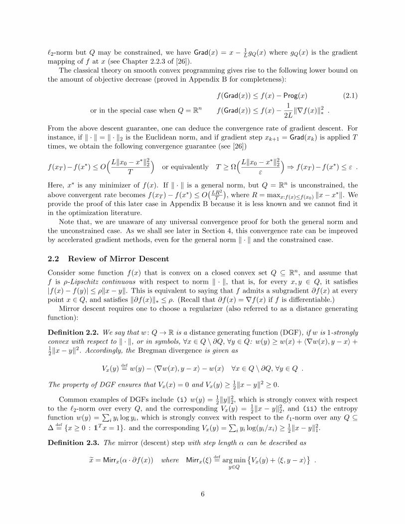
`2-norm but Q may be constrained, we have Grad(x) = x − 1LgQ(x) where gQ(x) is the gradient

mapping of f at x (see Chapter 2.2.3 of [26]).The classical theory on smooth convex programming gives rise to the following lower bound on

the amount of objective decrease (proved in Appendix B for completeness):

f(Grad(x)) ≤ f(x)− Prog(x) (2.1)

or in the special case when Q = Rn f(Grad(x)) ≤ f(x)− 1

2L‖∇f(x)‖2∗ .

From the above descent guarantee, one can deduce the convergence rate of gradient descent. Forinstance, if ‖ · ‖ = ‖ · ‖2 is the Euclidean norm, and if gradient step xk+1 = Grad(xk) is applied Ttimes, we obtain the following convergence guarantee (see [26])

f(xT )−f(x∗) ≤ O(L‖x0 − x∗‖22

T

)or equivalently T ≥ Ω

(L‖x0 − x∗‖22ε

)⇒ f(xT )−f(x∗) ≤ ε .

Here, x∗ is any minimizer of f(x). If ‖ · ‖ is a general norm, but Q = Rn is unconstrained, the

above convergent rate becomes f(xT )− f(x∗) ≤ O(LR2

T

), where R = maxx:f(x)≤f(x0) ‖x− x∗‖. We

provide the proof of this later case in Appendix B because it is less known and we cannot find itin the optimization literature.

Note that, we are unaware of any universal convergence proof for both the general norm andthe unconstrained case. As we shall see later in Section 4, this convergence rate can be improvedby accelerated gradient methods, even for the general norm ‖ · ‖ and the constrained case.

2.2 Review of Mirror Descent

Consider some function f(x) that is convex on a closed convex set Q ⊆ Rn, and assume thatf is ρ-Lipschitz continuous with respect to norm ‖ · ‖, that is, for every x, y ∈ Q, it satisfies|f(x)− f(y)| ≤ ρ‖x− y‖. This is equivalent to saying that f admits a subgradient ∂f(x) at everypoint x ∈ Q, and satisfies ‖∂f(x)‖∗ ≤ ρ. (Recall that ∂f(x) = ∇f(x) if f is differentiable.)

Mirror descent requires one to choose a regularizer (also referred to as a distance generatingfunction):

Definition 2.2. We say that w : Q→ R is a distance generating function (DGF), if w is 1-stronglyconvex with respect to ‖ · ‖, or in symbols, ∀x ∈ Q \ ∂Q, ∀y ∈ Q: w(y) ≥ w(x) + 〈∇w(x), y − x〉+12‖x− y‖2. Accordingly, the Bregman divergence is given as

Vx(y)def= w(y)− 〈∇w(x), y − x〉 − w(x) ∀x ∈ Q \ ∂Q, ∀y ∈ Q .

The property of DGF ensures that Vx(x) = 0 and Vx(y) ≥ 12‖x− y‖2 ≥ 0.

Common examples of DGFs include (i) w(y) = 12‖y‖22, which is strongly convex with respect

to the `2-norm over every Q, and the corresponding Vx(y) = 12‖x − y‖22, and (ii) the entropy

function w(y) =∑

i yi log yi, which is strongly convex with respect to the `1-norm over any Q ⊆∆

def= x ≥ 0 : 1Tx = 1. and the corresponding Vx(y) =

∑i yi log(yi/xi) ≥ 1

2‖x− y‖21.

Definition 2.3. The mirror (descent) step with step length α can be described as

x = Mirrx(α · ∂f(x)) where Mirrx(ξ)def= arg min

y∈Q

Vx(y) + 〈ξ, y − x〉

.

6

Mirror descent’s core lemma is the following inequality (proved in Appendix B for completeness):

If xk+1 = Mirrxk(α · ∂f(xk)

), then

∀u ∈ Q, α(f(xk)− f(u)) ≤ α〈∂f(xk), xk − u〉 ≤α2

2‖∂f(xk)‖2∗ + Vxk(u)− Vxk+1

(u) (2.2)

The term 〈∂f(xk), xk − u〉 features prominently in online optimization, and is known as the regretat iteration k with respect to u (see Appendix A.2 for the folklore relationship between mirrordescent and regret minimization). It is not hard to see that, telescoping (2.2) for k = 0, . . . , T − 1,

setting xdef= 1

T

∑T−1k=0 xk to be the average of the xk’s, and choosing u = x∗, we have

αT (f(x)− f(x∗)) ≤T−1∑

k=0

α〈∂f(xk), xk − x∗〉 ≤α2

2

T−1∑

k=0

‖∂f(xk)‖2∗ + Vx0(x∗)− VxT (x∗) . (2.3)

Finally, letting Θ be any upper bound on Vx0(x∗) (recall Θ = 12‖x0−x∗‖22 when ‖·‖ is the Euclidean

norm), and α =√

2Θρ·√T

be the step length, inequality (2.2) can be re-written as

f(x)− f(x∗) ≤√

2Θ · ρ√T

or equivalently T ≥ 2Θ · ρ2

ε2⇒ f(x)− f(x∗) ≤ ε . (2.4)

Remark. While their analyses share some similarities, mirror and gradient steps are often verydifferent. For example, if the optimization problem is over the simplex with `1 norm, then gradientstep gives x′ ← arg miny1

2‖y−x‖21+α〈∇f(x), y−x〉, while the mirror step with entropy regularizergives x′ ← arg miny

∑i yi log(yi/xi) + α〈∇f(x), y − x〉. We point out in Appendix A.1 that non-

Euclidean norms are very important for certain applications.In the special case of w(x) = 1

2‖x‖22 and ‖ · ‖ is `2-norm, gradient and mirror steps are indistin-guishable from each other. However, as we have discussed earlier, these two update rules are oftenequipped with very different convergence analyses, even if they ‘look the same’.

3 Warm-Up Method with Fixed Step Length

Consider the same setting as Section 2.1: that is, f(x) is convex and differentiable on its domain Q,and is L-smooth with respect to some norm ‖ · ‖. (Note that f(x) may not have a good Lipschitzcontinuity parameter ρ, but we do not need such a property.) In this section, we focus on theunconstrained case Q = Rn, and combine gradient and mirror descent to produce a very simpleaccelerated method. We explain this method first because it avoids the mysterious choices of steplengths as in the full setting, and carries our conceptual message in a very clean way.

Design an algorithm that, in every step k, performs both a gradient and a mirror step, andensures that the two steps are linearly coupled. More specifically, starting from x0 = y0 = z0, ineach iteration k = 0, 1, . . . , T − 1, we first define xk+1 ← τzk + (1− τ)yk and then• perform a gradient step yk+1 ← Grad(xk+1), and• perform a mirror step zk+1 ← Mirrzk

(α∇f(xk+1)

).9

Above, α is the (fixed) step length of the mirror step, while τ is the parameter controlling thecoupling rate. The choices of α and τ will become clear at the end of this section, but from a highlevel,• α will be determined from the mirror-descent analysis, similar to that in (2.3), and

9Here, the mirror step Mirr is defined by specifying any DGF w(·) that is 1-strongly convex over Q.

7

• τ will be determined as the best parameter to balance the gradient and mirror steps, similarto the “magic number” K in our thought experiment discussed in Section 1.3.

Classical gradient-descent and mirror-descent analyses immediately imply the following:

Lemma 3.1. For every u ∈ Q = Rn,

α〈∇f(xk+1), zk − u〉¬≤ α2

2‖∇f(xk+1)‖2∗ + Vzk(u)− Vzk+1

(u)

­≤ α2L

(f(xk+1)− f(yk+1)

)+ Vzk(u)− Vzk+1

(u) . (3.1)

Proof. To deduce ¬, we note that our mirror step zk+1 = Mirrzk(α∇f(xk+1)) is essentially identicalto that of xk+1 = Mirrxk(α∇f(xk)) in (2.2), with only changes of variable names. Therefore,inequality ¬ is a simple copy-and-paste from (2.2) after changing the variable names (see the proofof (2.2) for details). The second inequality ­ is from the gradient step guarantee f(xk+1)−f(yk+1) ≥1

2L‖∇f(xk+1)‖2∗ in (2.1). One can immediately see from Lemma 3.1 that, although the mirror step introduces an error

α2

2 ‖∇f(xk+1)‖2∗, this error is proportional to the amount of the gradient-step progress f(xk+1) −f(yk+1). This captures the observation we stated in the introduction: if ‖∇f(xk+1)‖∗ is large, wecan make a large gradient step, or if ‖∇f(xk+1)‖∗ is small, the mirror step suffers from a small loss.

If we choose τ = 1 or equivalently xk+1 = zk, the left hand side of inequality (3.1) becomes〈∇f(xk+1), xk+1 − u〉, the regret at iteration xk+1. In such a case we wish to telescope it for alliterations k in the spirit of mirror descent (see (2.3)). However, we face the problem that the termsf(xk+1) − f(yk+1) do not telescope. 10 On the other hand, if we choose τ = 0 or equivalentlyxk+1 = yk, then the terms f(xk+1)− f(yk+1) = f(yk)− f(yk+1) telescope, but the left hand side of(3.1) is no longer the regret. 11

To overcome this issue, we use linear coupling. We compute and upper bound the differencebetween the left hand side of (3.1) and the actual “regret”:

α〈∇f(xk+1), xk+1 − u〉 − α〈∇f(xk+1), zk − u〉

= α〈∇f(xk+1), xk+1 − zk〉 =(1− τ)α

τ〈∇f(xk+1), yk − xk+1〉 ≤

(1− τ)α

τ(f(yk)− f(xk+1)). (3.2)

Above, we used the fact that τ(xk+1− zk) = (1− τ)(yk − xk+1), as well as the convexity of f(·). Itis now immediate that by choosing 1−τ

τ = αL and combining (3.1) and (3.2), we have

Lemma 3.2 (Coupling). Letting τ ∈ (0, 1) satisfy that 1−ττ = αL, we have that

∀u ∈ Q = Rn, α〈∇f(xk+1), xk+1 − u〉 ≤ α2L(f(yk)− f(yk+1)

)+(Vzk(u)− Vzk+1

(u)).

It is clear from the above proof that τ is introduced to precisely balance the objective decreasef(xk+1) − f(yk+1), and the (possible) objective increase f(yk) − f(xk+1). This is similar to the“magic number” K discussed in the introduction.

Finally Convergence Rate. We telescope inequality Lemma 3.2 for k = 0, 1, . . . , T − 1. Settingx

def= 1

T

∑T−1k=0 xk and u = x∗, we have

αT (f(x)− f(x∗)) ≤T−1∑

k=0

α〈∂f(xk), xk − x∗〉 ≤ α2L(f(y0)− f(yT )

)+ Vx0(x∗)− VxT (x∗) . (3.3)

10In other words, although a gradient step may decrease the objective from f(xk+1) to f(yk+1), it may also getthe objective increased from f(yk) to f(xk+1).

11Indeed, our “thought experiment” in the introduction is conducted as if we both had xk+1 = zk and xk+1 = yk,and therefore we could arrive at the upcoming (3.3) directly.

8

Suppose our initial point is of error at most d, that is f(y0)− f(x∗) ≤ d, and suppose Vx0(x∗) ≤ Θ,then (3.3) gives f(x)−f(x∗) ≤ 1

T

(αLd+Θ/α

). Choosing α =

√Θ/Ld to be the value that balances

the above two terms,12 we obtain that f(x)− f(x∗) ≤ 2√LΘdT . In other words,

in T = 4√LΘ/d steps, we can obtain some x satisfying f(x)− f(x∗) ≤ d/2,

halving the distance to the optimum. If we restart this entire procedure a few number of times,halving the distance for every run, then we obtain an ε-approximate solution in

T = O(√

LΘ/ε+√LΘ/2ε+

√LΘ/4ε+ · · ·

)= O

(√LΘ/ε

)

iterations, matching the same running time of Nesterov’s accelerated methods [25–27]. It is im-portant to note here that α =

√Θ/Ld increases as time goes (i.e., as d goes down), and therefore

τ = 1αL+1 decreases as time goes. This lesson instructs us that gradient steps should be given more

weights than mirror steps, when it is closer to the optimum.13

Conclusion. Equipped with the basic knowledge of gradient descent and mirror descent, theabove proof is quite straightforward and gives intuition on how the two “magic numbers” α andτ are selected. However, this simple algorithm has several caveats. First, the value α dependson the knowledge of Θ; second, a good initial distance bound d has to be specified; and third,the algorithm has to be restarted. In the next section, we let α and τ change gradually acrossiterations. This overcomes the mentioned caveats, and also extends the above analysis to allow Qto be constrained.

4 Final Method with Variable Step Lengths

In this section, we recover the main result of [27] in the constrained case, that is

Theorem 4.1. If f(x) is L-smooth w.r.t. ‖ · ‖ on Q, and w(x) is 1-strongly convex w.r.t. ‖ · ‖on Q, then AGM outputs yT satisfying f

(yT)− f(x∗) ≤ 4ΘL/T 2, where Θ is any upper bound on

Vx0(x∗).

We remark here that it is very important to allow the norm ‖ · ‖ to be general, rather than focusingon the `2-norm as in [26]. See our discussion in Appendix A.1.

Our algorithm AGM (see Algorithm 1) starts from x0 = y0 = z0. In each step k = 0, 1, . . . , T − 1,it computes xk+1 ← τkzk + (1− τk)yk and then• performs gradient step yk+1 ← Grad(xk+1), and• performs mirror step zk+1 ← Mirrzk

(αk+1∇f(xk+1)

).

Here, αk+1 is the step length of mirror descent and will be chosen at the end of this section. Thevalue τk is 1

αk+1Lwhich is slightly different from 1

αL+1 used in the warm-up case. (This is necessary

to capture the constrained case.) Our choice of αk+1 will ensure that τk ∈ (0, 1] for each k.

Convergence Analysis. We state the analogue of Lemma 3.1 whose proof is in Appendix C:

12This is essentially the same way to choose α in mirror descent, see (2.3).13One may find this counter-intuitive because when it is closer to the optimum, the observed gradients will become

smaller, and therefore mirror steps should perform well due to our conceptual message in the introduction. Thisunderstanding is incorrect for two reasons. First, when it is closer to the optimum, the threshold between “large”and “small” gradients also become smaller, so one cannot rely only on mirror steps. Second, when it is closer tothe optimum, mirror steps are more ‘unstable’ and may increase the objective more (in comparison to the currentdistance to the optimum), and thus should be given less weight.

9

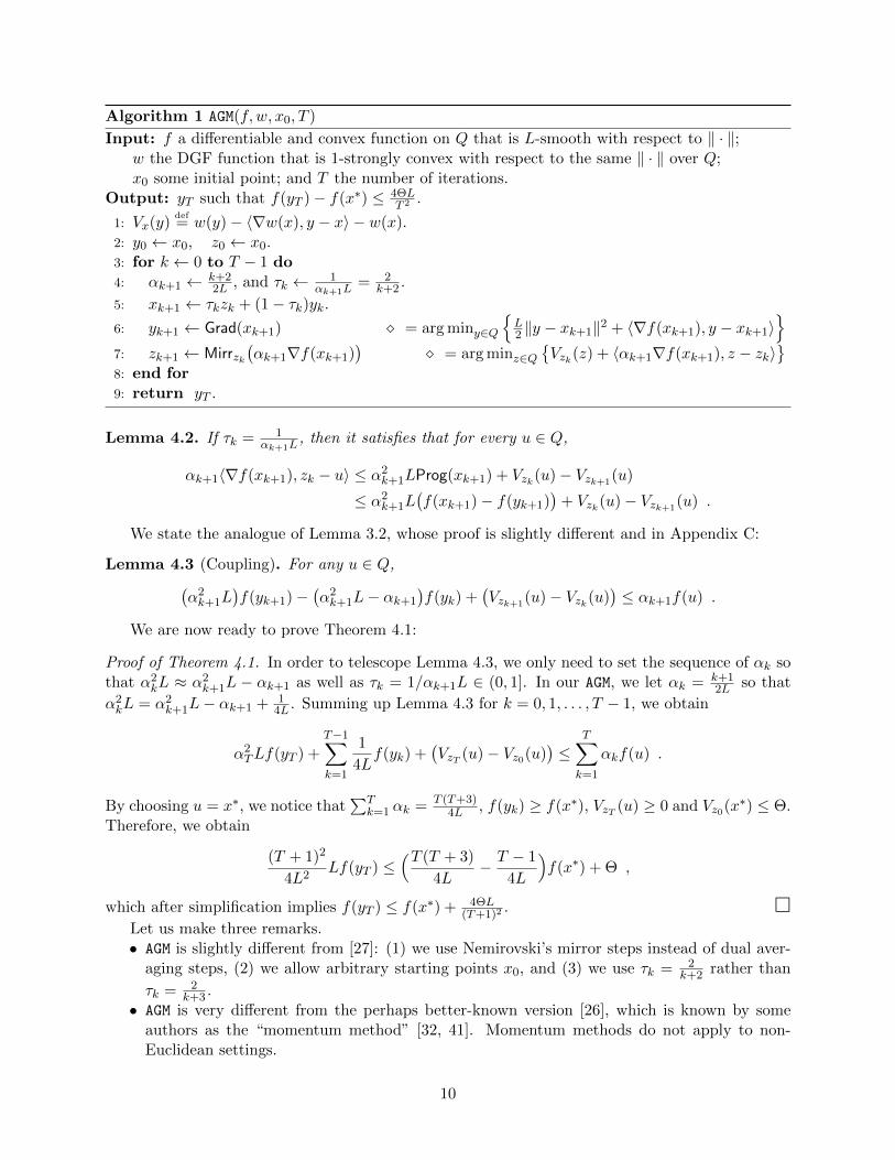
Algorithm 1 AGM(f, w, x0, T )

Input: f a differentiable and convex function on Q that is L-smooth with respect to ‖ · ‖;w the DGF function that is 1-strongly convex with respect to the same ‖ · ‖ over Q;x0 some initial point; and T the number of iterations.

Output: yT such that f(yT )− f(x∗) ≤ 4ΘLT 2 .

1: Vx(y)def= w(y)− 〈∇w(x), y − x〉 − w(x).

2: y0 ← x0, z0 ← x0.3: for k ← 0 to T − 1 do4: αk+1 ← k+2

2L , and τk ← 1αk+1L

= 2k+2 .

5: xk+1 ← τkzk + (1− τk)yk.6: yk+1 ← Grad(xk+1) = arg miny∈Q

L2 ‖y − xk+1‖2 + 〈∇f(xk+1), y − xk+1〉

7: zk+1 ← Mirrzk(αk+1∇f(xk+1)

) = arg minz∈Q

Vzk(z) + 〈αk+1∇f(xk+1), z − zk〉

8: end for9: return yT .

Lemma 4.2. If τk = 1αk+1L

, then it satisfies that for every u ∈ Q,

αk+1〈∇f(xk+1), zk − u〉 ≤ α2k+1LProg(xk+1) + Vzk(u)− Vzk+1

(u)

≤ α2k+1L

(f(xk+1)− f(yk+1)

)+ Vzk(u)− Vzk+1

(u) .

We state the analogue of Lemma 3.2, whose proof is slightly different and in Appendix C:

Lemma 4.3 (Coupling). For any u ∈ Q,(α2k+1L

)f(yk+1)−

(α2k+1L− αk+1

)f(yk) +

(Vzk+1

(u)− Vzk(u))≤ αk+1f(u) .

We are now ready to prove Theorem 4.1:

Proof of Theorem 4.1. In order to telescope Lemma 4.3, we only need to set the sequence of αk sothat α2

kL ≈ α2k+1L − αk+1 as well as τk = 1/αk+1L ∈ (0, 1]. In our AGM, we let αk = k+1

2L so that

α2kL = α2

k+1L− αk+1 + 14L . Summing up Lemma 4.3 for k = 0, 1, . . . , T − 1, we obtain

α2TLf(yT ) +

T−1∑

k=1

1

4Lf(yk) +

(VzT (u)− Vz0(u)

)≤

T∑

k=1

αkf(u) .

By choosing u = x∗, we notice that∑T

k=1 αk = T (T+3)4L , f(yk) ≥ f(x∗), VzT (u) ≥ 0 and Vz0(x∗) ≤ Θ.

Therefore, we obtain

(T + 1)2

4L2Lf(yT ) ≤

(T (T + 3)

4L− T − 1

4L

)f(x∗) + Θ ,

which after simplification implies f(yT ) ≤ f(x∗) + 4ΘL(T+1)2

. Let us make three remarks.• AGM is slightly different from [27]: (1) we use Nemirovski’s mirror steps instead of dual aver-

aging steps, (2) we allow arbitrary starting points x0, and (3) we use τk = 2k+2 rather than

τk = 2k+3 .

• AGM is very different from the perhaps better-known version [26], which is known by someauthors as the “momentum method” [32, 41]. Momentum methods do not apply to non-Euclidean settings.

10

• In Appendix D, we also recover the strong convexity version of accelerated gradient meth-ods [26], and thus linear coupling provides a complete proof of all existing accelerated gradientmethods.

5 Beyond Accelerated Gradient Methods

Providing an intuitive, yet complete interpretation of accelerated gradient methods is an openquestion in Optimization [17]. Our result in this paper is one important step towards this generalgoal. Linear coupling not only gives a reinterpretation of Nesterov’s accelerated methods, moreimportantly, it provides a framework for designing first-order methods in a bigger agenda. Sincethe original version of this paper appeared online, our linear-coupling framework has led to break-throughs for several problems in computer science. In all such problems, the original Nesterov’saccelerated methods do not apply. We illustrate a few examples in this line of research, in order todemonstrate the power and generality of linear coupling.

Recall the key lemmas of gradient and mirror descent in linear coupling (see (3.1)):

gradient descent: f(xk+1)− f(yk+1) ≥ 1

2L‖∇f(xk+1)‖2∗ (5.1)

mirror descent: α〈∇f(xk+1), zk − u〉 ≤α2

2‖∇f(xk+1)‖2∗ + Vzk(u)− Vzk+1

(u) (5.2)

Extension 1: Strengthening (5.2) and (5.1). If f satisfies good properties other than smooth-ness, one can also develop objective decrease lemma to replace (5.1). In addition, if necessary, anon-strongly convex regularizer can be used in mirror descent to replace (5.2). In either or bothsuch cases, linear coupling can still be used to combine the two methods and obtain faster runningtimes; in contrast, Nesterov’s original accelerated methods do not apply.

For example, recent breakthroughs on positive linear programming (positive LP) are all basedon the above extension of linear coupling [3–5, 22, 42, 43]. For such LPs, the correspondingobjective f is intrinsically non-smooth. Some authors including Nesterov himself have appliedsimple smoothing to turn f into a smooth variant f ′, and then minimized f ′ [27]; however, evenif Nesterov’s accelerated methods are used to minimize f ′, the resulting running time scales withthe problem’s width, a parameter that can be exponential in input size.14 In contrast, if linearcoupling is used, one can show that f(xk+1) − f(yk+1) is lower bounded by a constant times∑

j max|∇jf(xk+1)|, 12 for the original objective f (see [4]). This is a weaker version of (5.1).However, after linear coupling, it leads to a faster algorithm than naively applying Nesterov’saccelerated methods on f ′ in all parameter regimes.

Extension 2: Three-Point Coupling. One may naturally consider linearly coupling for morethan two vectors. While this is provably unnecessary for minimizing a smooth objective in thefull-gradient setting (because accelerated gradient methods are already optimal), it can be veryhelpful in the stochastic-gradient setting.

More specifically, it was a known obstacle in Nesterov’s accelerated methods (including ourAGM) that if the full gradient ∇f(xk+1) is replaced with a random estimator ∇ whose expectationE[∇] = ∇f(xk+1), then acceleration disappears in the worst case. Using linear coupling, we canfix this issue by providing the first direct accelerated stochastic gradient method. In [1], the author

14We recommend interested readers to find detailed discussions in [4] regarding the importance of designing width-independent solvers for positive LP. As an illustrative example, in the problem of maximum matching (which can bewritten as positive LP), the width of the problem is the number of edges in the graph.

11

replaced the coupling step xk+1 ← τzk + (1 − τ)yk with xk+1 ← τ1zk + τ2x + (1 − τ2 − τ1)yk,where x is a snapshot point whose full gradient is computed exactly but very infrequently. Such a“three-point” linear coupling provides an accelerated running time because one can combine (5.1),(5.2), together with a so-called variance-reduction inequality [16] all three at once.

Extension 3: Optimal Sampling Probability. Nesterov’s accelerated methods generalize tocoordinate-descent settings, that is, to minimize f that is Li-smooth for each coordinate i. Thebest known coordinate-descent method [21] samples each coordinate i with probability proportionalto Li, and is based on a randomized version of Nesterov’s original analysis. Using linear coupling,the authors of [6] discovered that one should select i with probability proportional to

√Li for an

even faster running time.To illustrate the reasoning behind this, let us revisit (5.1) and (5.2). In the coordinate-descent

setting, if we abbreviate xk+1 with x, the right hand side of (5.1) simply becomes 12Li

(∇if(x))2 ifcoordinate i is selected. As for (5.2), to ensure its left hand side stays the same in expectation, oneshould replace ∇f(x) with 1

pi∇if(x), where pi is the probability to select i. As a result, the first

term on the right hand side of (5.2) becomes α2

2p2i(∇if(x))2. By comparing these two new terms

12Li

(∇if(x))2 and α2

2p2i(∇if(x))2, we immediately notice that pi had better be proportional to

√Li

in order for the two terms to cancel. This simple idea, fully motivated from linear coupling, leadsto the fastest accelerated coordinate-descent method [6].

Extension 4: Supporting Non-Convexity. Consider objectives f that are not even convexbut still smooth. For instance, neural network training objectives fall into this class if smoothedactivation functions are used. In such a case, both (5.1) and (5.2) remain true. However, whencoupling the two steps, we cannot claim 〈∇f(xk+1), xk+1 − u〉 ≥ f(xk+1) − f(u) because thereis no convexity. In [2], the authors discovered that one can use the quadratic lower bound〈∇f(xk+1), xk+1 − u〉 ≥ f(xk+1) − f(u) − L

2 ‖xk+1 − u‖2 to replace convexity arguments, and stillperform a weaker version of linear coupling. This leads to a stochastic algorithm that converges toapproximate saddle-points,15 outperforming both gradient descent and stochastic gradient descent,the only two known first-order methods with provably convergence guarantees.

Acknowledgements

We thank Jon Kelner and Yin Tat Lee for helpful conversations, and Aaditya Ramdas for pointingout a typo in the previous version of this paper.

This material is based upon work partly supported by the National Science Foundation underGrant CCF-1319460 and by a Simons Graduate Student Award under grant no. 284059.

15Recall that in general non-convex optimization one can only hope for converging to saddle-points.

12

Appendix

A Several Remarks on First-Order Methods

A.1 Importance of Non-Euclidean Norms

Let us use a simple example to illustrate the importance of allowing arbitrary norms in studyingfirst-order methods.

Consider the saddle point problem of minx∈∆n maxy∈∆m yTAx, where A is an m × n matrix,

∆n = x ∈ Rn : x ≥ 0 ∧ 1Tx = 1 is the unit simplex in Rn, and ∆m = y ∈ Rm : y ≥ 0 ∧ 1T y =1. This problem is important to study because it captures packing and covering linear programsthat have wide applications in many areas of computer science (see the survey of [8]).

Letting µ = ε2 logm , Nesterov has shown that the following objective

fµ(x)def= µ log

( 1

m

m∑

j=1

exp1µ

(Ax)j),

when optimized over x ∈ ∆n, can yield an additive ε/2 solution to the original saddle pointproblem [27].

This fµ(x) is proven to be 1µ -smooth with respect to the `1-norm over ∆n, if all the entries

of A are between [−1, 1]. Instead, fµ(x) is 1µ -smooth with respect to the `2-norm over ∆n, only

if the sum of squares of every row of A is at most 1. This `2 condition is certainly stronger andless natural than the `1 condition, and the `1 condition one leads to the fastest (approximate)width-dependent positive LP solver [27].

Different norm conditions also yield different gradient and mirror descent steps. For instance,in the `1-norm case, the gradient step is x′ ← arg minx′∈∆n

12‖x′ − x‖21 + α〈∇fµ(x), x′ − x〉

, and

the mirror step is x′ ← arg minx′∈∆n

∑i∈[n] x

′i log

x′ixi

+ α〈∇fµ(x), x′ − x〉

. In the `2-norm case,

gradient and mirror steps are both of the form x′ ← arg minx′∈∆n

12‖x′−x‖22 +α〈∇fµ(x), x′−x〉

.

As another example, [35] has shown that the `1 norm, instead of the `2 one, is crucial whencomputing the minimum enclosing ball of points. One can find other applications as well in [27]for the use of non-Euclidean norms, and an interesting example of `∞-norm gradient descent fornearly-linear time maximum flow in [18].

It is now important to note that, the methods in [25, 26] work only for the `2-norm case, andit is not clear how the proof can be generalized to other norms until [27]. Some other proofs (suchas [13]) only work for the `2-norm because the mirror steps are described as (a scaled version of)gradient steps.

A.2 Folklore Relationship Between Multiplicative Weight Updates and MirrorDescent

The multiplicative weight update (MWU) method (see the survey of Arora, Hazan and Kale [8]) isa simple method that has been repeatedly discovered in theory of computation, machine learning,optimization, and game theory. The setting of this method is the following.

Let ∆n = x ∈ Rn : x ≥ 0 ∧ 1Tx = 1 be the unit simplex in Rn, and we call any vector in∆n an action. A player is going to play T actions x0, . . . , xT−1 ∈ ∆n in a row; only after playingxk, the player observes a loss vector `k ∈ Rn that may depend on xk, and suffers from a loss value

13

〈`k, xk〉. The MWU method ensures that, if ‖`k‖∞ ≤ ρ for all k ∈ [T ], then the player has an(adaptive) strategy to choose the actions such that the average regret is bounded:

1

T

( T−1∑

i=0

〈`k, xk〉 − minu∈∆n

T−1∑

i=0

〈`k, u〉)≤ O

(ρ√log n√T

). (A.1)

The left hand side is called the average regret because it is the (average) difference between thesuffered loss

∑T−1i=0 〈`k, xk〉, and the loss

∑T−1i=0 〈`k, u〉 of the best action u ∈ ∆n in hindsight. Another

way to interpret (A.1) is to state that we can obtain an average regret of ε using T = O(ρ2 lognε2

)rounds.

The above result can be proven directly using mirror descent. Letting w(x)def=∑

i xi log xi be

the entropy DGF over the simplex Q = ∆n, and its corresponding Bregman divergence Vx(x′) def=∑

i∈[n] x′i log

x′ixi

, we consider the following update rule.

Start from x0 = (1/n, . . . , 1/n), and update xk+1 = Mirrxk(α`k), or equivalently, xk+1,i =

xk,i · exp−α`k,i /Zk, where Zk > 0 is the normalization factor that equals to∑n

i=1 xk,i · exp−α`k,i .16

Then, the mirror-descent guarantee (2.2) implies that17

∀u ∈ ∆n, α〈`k, xk − u〉 ≤α2

2‖`k‖2∞ + Vxk(u)− Vxk+1

(u) .

After telescoping the above inequality for all k = 0, 1, . . . , T − 1, and using the upper bounds‖`(xk)‖∞ ≤ ρ and Vx0(u) ≤ log n, we obtain that for all u ∈ ∆n,

1

T

T−1∑

k=0

〈`k, xk − u〉 ≤αρ2

2+

log n

αT.

Setting α =√

logn

ρ√T

we arrive at the desired average regret bound (A.1).

In sum, we have re-deduced the MWU method from mirror descent, and the above proofis quite different from most of the classical analysis of MWU (e.g., [7, 8, 14, 34]). It can begeneralized to solve the matrix version of MWU [8, 33], as well as to incorporate the width-reduction technique [8, 34]. We ignore such extensions here because they are outside the scope ofthis paper.

A.3 Deducing the Mirror-Descent Guarantee via Gradient Descent

In this section, we re-deduce the convergence rate of mirror descent from gradient descent. Inparticular, we show that the dual averaging steps are equivalent to gradient steps on the Fencheldual of the regularized regret, and deduce the same convergence bound as (2.4). (Similar proof canalso be obtained for mirror steps but is notationally more involved.)

Given a sequence of points x0, . . . , xT−1 ∈ Q, the (scaled) regret with respect to any point

u ∈ Q is R(x0, . . . , xT−1, u)def=∑T−1

i=0 α〈∂f(xi), xi − u〉. Since it satisfies that αT · (f(x)− f(u)) ≤16This version of the MWU is often known as the Hedge rule [14]. Another commonly used version is to choose

xk+1,i =xk,i(1−α`k,i)

Zk. Since e−t ≈ 1 − t whenever |t| is small and our choice of α will make sure that |α`k,i| 1,

this is essentially identical to the Hedge rule.17To be precise, we have replaced ∂f(xk) with `k. It is easy to see from the proof of (2.2) that this loss vector `k

does not need to come from the subgradient of some objective f(·).

14

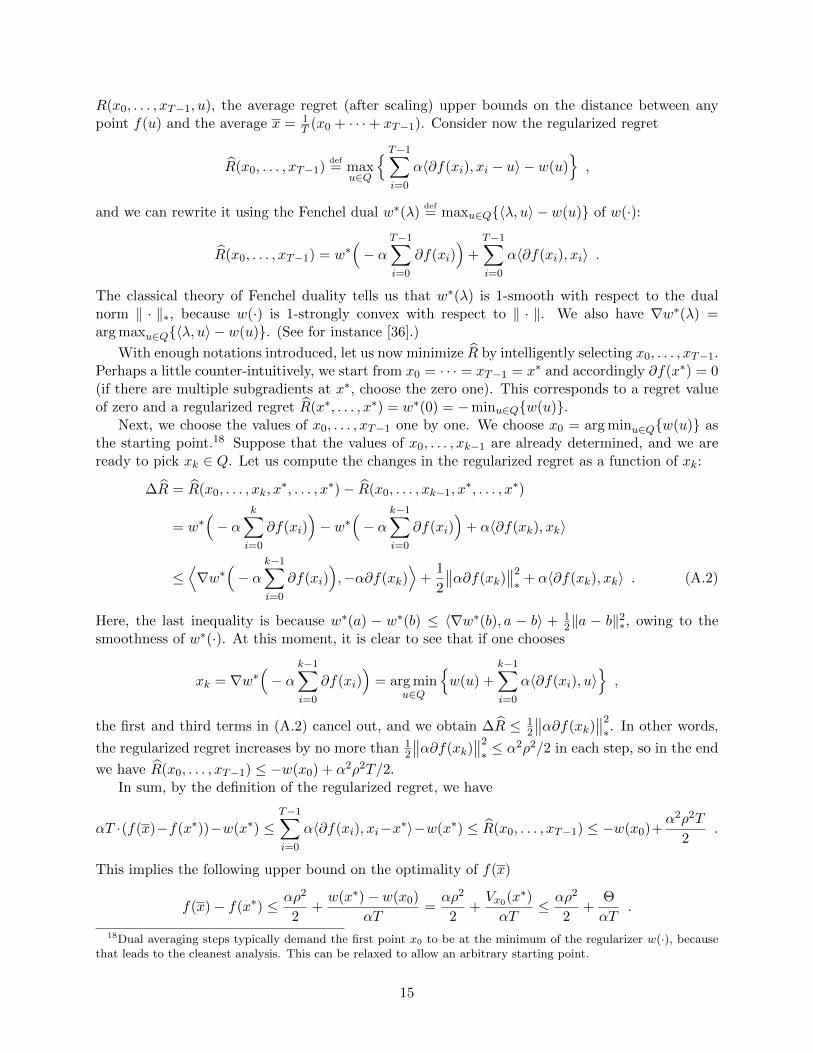
R(x0, . . . , xT−1, u), the average regret (after scaling) upper bounds on the distance between anypoint f(u) and the average x = 1

T (x0 + · · ·+ xT−1). Consider now the regularized regret

R(x0, . . . , xT−1)def= max

u∈Q

T−1∑

i=0

α〈∂f(xi), xi − u〉 − w(u),

and we can rewrite it using the Fenchel dual w∗(λ)def= maxu∈Q〈λ, u〉 − w(u) of w(·):

R(x0, . . . , xT−1) = w∗(− α

T−1∑

i=0

∂f(xi))

+T−1∑

i=0

α〈∂f(xi), xi〉 .

The classical theory of Fenchel duality tells us that w∗(λ) is 1-smooth with respect to the dualnorm ‖ · ‖∗, because w(·) is 1-strongly convex with respect to ‖ · ‖. We also have ∇w∗(λ) =arg maxu∈Q〈λ, u〉 − w(u). (See for instance [36].)

With enough notations introduced, let us now minimize R by intelligently selecting x0, . . . , xT−1.Perhaps a little counter-intuitively, we start from x0 = · · · = xT−1 = x∗ and accordingly ∂f(x∗) = 0(if there are multiple subgradients at x∗, choose the zero one). This corresponds to a regret valueof zero and a regularized regret R(x∗, . . . , x∗) = w∗(0) = −minu∈Qw(u).

Next, we choose the values of x0, . . . , xT−1 one by one. We choose x0 = arg minu∈Qw(u) asthe starting point.18 Suppose that the values of x0, . . . , xk−1 are already determined, and we areready to pick xk ∈ Q. Let us compute the changes in the regularized regret as a function of xk:

∆R = R(x0, . . . , xk, x∗, . . . , x∗)− R(x0, . . . , xk−1, x

∗, . . . , x∗)

= w∗(− α

k∑

i=0

∂f(xi))− w∗

(− α

k−1∑

i=0

∂f(xi))

+ α〈∂f(xk), xk〉

≤⟨∇w∗

(− α

k−1∑

i=0

∂f(xi)),−α∂f(xk)

⟩+

1

2

∥∥α∂f(xk)∥∥2

∗ + α〈∂f(xk), xk〉 . (A.2)

Here, the last inequality is because w∗(a) − w∗(b) ≤ 〈∇w∗(b), a − b〉 + 12‖a − b‖2∗, owing to the

smoothness of w∗(·). At this moment, it is clear to see that if one chooses

xk = ∇w∗(− α

k−1∑

i=0

∂f(xi))

= arg minu∈Q

w(u) +

k−1∑

i=0

α〈∂f(xi), u〉,

the first and third terms in (A.2) cancel out, and we obtain ∆R ≤ 12

∥∥α∂f(xk)∥∥2

∗. In other words,

the regularized regret increases by no more than 12

∥∥α∂f(xk)∥∥2

∗ ≤ α2ρ2/2 in each step, so in the end

we have R(x0, . . . , xT−1) ≤ −w(x0) + α2ρ2T/2.In sum, by the definition of the regularized regret, we have

αT ·(f(x)−f(x∗))−w(x∗) ≤T−1∑

i=0

α〈∂f(xi), xi−x∗〉−w(x∗) ≤ R(x0, . . . , xT−1) ≤ −w(x0)+α2ρ2T

2.

This implies the following upper bound on the optimality of f(x)

f(x)− f(x∗) ≤ αρ2

2+w(x∗)− w(x0)

αT=αρ2

2+Vx0(x∗)αT

≤ αρ2

2+

Θ

αT.

18Dual averaging steps typically demand the first point x0 to be at the minimum of the regularizer w(·), becausethat leads to the cleanest analysis. This can be relaxed to allow an arbitrary starting point.

15

Finally, choosing α =√

2Θρ·√T

to be the step length, we arrive at f(x) − f(x∗) ≤√

2Θ·ρ√T

, which is the

same convergence rate as (2.4).

B Missing Proof of Section 2

For the sake of completeness, we provide self-contained proofs of the mirror descent and mirrordescent guarantees in this section.

B.1 Missing Proof for Gradient Descent

Gradient Descent Guarantee

f(Grad(x)) ≤ f(x)− Prog(x) (2.1)

or in the special case when Q = Rn f(Grad(x)) ≤ f(x)− 1

2L‖∇f(x)‖2∗ .

Proof. 19 Letting x = Grad(x), we prove the first inequality by

Prog(x) = −miny∈Q

L2‖y − x‖2 + 〈∇f(x), y − x〉

= −

(L2‖x− x‖2 + 〈∇f(x), x− x〉

)

= f(x)−(L

2‖x− x‖2 + 〈∇f(x), x− x〉+ f(x)

)≤ f(x)− f(x) .

Here, the last inequality is a consequence of the smoothness assumption: for any x, y ∈ Q,

f(y)− f(x) =

∫ 1

τ=0〈∇f(x+ τ(y − x)), y − x〉dτ

= 〈∇f(x), y − x) +

∫ 1

τ=0〈∇f(x+ τ(y − x))−∇f(x), y − x〉dτ

≤ 〈∇f(x), y − x) +

∫ 1

τ=0‖∇f(x+ τ(y − x))−∇f(x)‖∗ · ‖y − x‖dτ

≤ 〈∇f(x), y − x) +

∫ 1

τ=0τL‖y − x‖ · ‖y − x‖dτ = 〈∇f(x), y − x〉+

L

2‖y − x‖2

The second inequality follows because in the special case of Q = Rn, we have

Prog(x) = −miny∈Q

L2‖y − x‖2 + 〈∇f(x), y − x〉

=

1

2L‖∇f(x)‖2∗ .

Fact B.1 (Gradient Descent Convergence). Let f(x) be a convex, differentiable function that isL-smooth with respect to ‖ · ‖ on Q = Rn, and x0 any initial point in Q. Consider the sequence ofT gradient steps xk+1 ← Grad(xk), then the last point xT satisfies that

f(xT )− f(x∗) ≤ O(LR2

T

),

where R = maxx:f(x)≤f(x0) ‖x− x∗‖, and x∗ is any minimizer of f .

19This proof can be found for instance in the textbook [26].

16

Proof. 20 Recall that we have f(xk+1) ≤ f(xk) − 12L‖∇f(xk)‖2∗ from (2.1). Furthermore, by the

convexity of f and Cauchy-Schwarz we have

f(xk)− f(x∗) ≤ 〈∇f(xk), xk − x∗〉 ≤ ‖∇f(xk)‖∗ · ‖xk − x∗‖ ≤ R · ‖∇f(xk)‖∗ .

Letting Dk = f(xk)− f(x∗) denote the distance to the optimum at iteration k, we now obtain tworelationships Dk −Dk+1 ≥ 1

2L‖∇f(xk)‖2∗ as well as Dk ≤ R · ‖∇f(xk)‖∗. Combining these two, weget

D2k ≤ 2LR2(Dk −Dk+1) =⇒ Dk

Dk+1≤ 2LR2

( 1

Dk+1− 1

Dk

).

Noticing that Dk ≥ Dk+1 because our objective only decreases at every round, we obtain that1

Dk+1− 1

Dk≥ 1

2LR2 . Finally, we conclude that at round T , we must have 1DT≥ T

2LR2 , finishing the

proof that f(xT )− f(x∗) ≤ 2LR2

T .

B.2 Missing Proof for Mirror Descent

Mirror Descent Guarantee

If xk+1 = Mirrxk(α · ∂f(xk)

), then

∀u ∈ Q, α(f(xk)− f(u)) ≤ α〈∂f(xk), xk − u〉 ≤α2

2‖∂f(xk)‖2∗ + Vxk(u)− Vxk+1

(u) . (2.2)

Proof. 21 we compute that

α〈∂f(xk), xk − u〉 = 〈α∂f(xk), xk − xk+1〉+ 〈α∂f(xk), xk+1 − u〉¬≤ 〈α∂f(xk), xk − xk+1〉+ 〈−∇Vxk(xk+1), xk+1 − u〉­= 〈α∂f(xk), xk − xk+1〉+ Vxk(u)− Vxk+1

(u)− Vxk(xk+1)

®≤(〈α∂f(xk), xk − xk+1〉 −

1

2‖xk − xk+1‖2

)+(Vxk(u)− Vxk+1

(u))

¯≤ α2

2‖∂f(xk)‖2∗ +

(Vxk(u)− Vxk+1

(u))

Here, ¬ is due to the minimality of xk+1 = arg minx∈QVxk(x) + 〈α∂f(xk), x〉, which implies that〈∇Vxk(xk+1) + α∂f(xk), u− xk+1〉 ≥ 0 for all u ∈ Q. ­ is due to the triangle equality of Bregmandivergence.22 ® is because Vx(y) ≥ 1

2‖x − y‖2 by the strong convexity of the DGF w(·). ¯ is byCauchy-Schwarz.

20Our proof follows almost directly from [26], but he only uses the Euclidean `2 norm.21This proof can be found for instance in the textbook [9].22 That is,

∀x, y ≥ 0, 〈−∇Vx(y), y − u〉 = 〈∇w(x)−∇w(y), y − u〉= (w(u)− w(x)− 〈∇w(x), u− x〉)− (w(u)− w(y)− 〈∇w(y), u− y)〉)− (w(y)− w(x)− 〈∇w(x), y − x〉)

= Vx(u)− Vy(u)− Vx(y) .

17

C Missing Proofs of Section 4

Lemma 4.2. If τk = 1αk+1L

, then it satisfies that for every u ∈ Q,

αk+1〈∇f(xk+1), zk − u〉¬≤ α2

k+1LProg(xk+1) + Vzk(u)− Vzk+1(u)

­≤ α2

k+1L(f(xk+1)− f(yk+1)

)+ Vzk(u)− Vzk+1

(u) .

Proof. The second inequality ­ is again from the gradient descent guarantee f(xk+1)− f(yk+1) ≥Prog(xk+1). To prove ¬, we first write down the key inequality of mirror-descent analysis (whoseproof is identical to that of (2.2))

αk+1〈∇f(xk+1), zk − u〉 = 〈αk+1∇f(xk+1), zk − zk+1〉+ 〈αk+1∇f(xk+1), zk+1 − u〉¬≤ 〈αk+1∇f(xk+1), zk − zk+1〉+ 〈−∇Vzk(zk+1), zk+1 − u〉­= 〈αk+1∇f(xk+1), zk − zk+1〉+ Vzk(u)− Vzk+1

(u)− Vzk(zk+1)

®≤(〈αk+1∇f(xk+1), zk − zk+1〉 −

1

2‖zk − zk+1‖2

)+(Vzk(u)− Vzk+1

(u))

Here, ¬ is due to the minimality of zk+1 = arg minz∈QVzk(z) + 〈αk+1∇f(xk+1), z〉, which impliesthat 〈∇Vzk(zk+1) + αk+1∇f(xk+1), u − zk+1〉 ≥ 0 for all u ∈ Q. ­ is due to the triangle equalityof Bregman divergence (see Footnote 22 in Appendix B). ® is because Vx(y) ≥ 1

2‖x − y‖2 by thestrong convexity of the w(·).

If one stops here and uses Cauchy-Shwartz 〈αk+1∇f(xk+1), zk − zk+1〉 − 12‖zk − zk+1‖2 ≤

α2k+1

2 ‖∇f(xk+1)‖2∗, he will get the desired inequality in the special case of Q = Rn, becauseProg(xk+1) = 1

2L‖∇f(xk+1)‖2∗ from (2.1).For the general unconstrained case, we need to use the special choice of τk = 1/αk+1L follows.

Letting vdef= τkzk+1 + (1− τk)yk ∈ Q so that xk+1− v = (τkzk + (1− τk)yk)− v = τk(zk − zk+1), we

have

〈αk+1∇f(xk+1), zk − zk+1〉 −1

2‖zk − zk+1‖2

= 〈αk+1

τk∇f(xk+1), xk+1 − v〉 −

1

2τ2k

‖xk+1 − v‖2

= α2k+1L

(〈∇f(xk+1), xk+1 − v〉 −

L

2‖xk+1 − v‖2

)≤ α2

k+1LProg(xk+1)

where the last inequality is from the definition of Prog(xk+1). Lemma 4.3 (Coupling). For any u ∈ Q,

(α2k+1L

)f(yk+1)−

(α2k+1L− αk+1

)f(yk) +

(Vzk+1

(u)− Vzk(u))≤ αk+1f(u) .

18

Proof. We deduce the following sequence of inequalities

αk+1

(f(xk+1)− f(u)

)

≤ αk+1〈∇f(xk+1), xk+1 − u〉= αk+1〈∇f(xk+1), xk+1 − zk〉+ αk+1〈∇f(xk+1), zk − u〉¬=

(1− τk)αk+1

τk〈∇f(xk+1), yk − xk+1〉+ αk+1〈∇f(xk+1), zk − u〉

­≤ (1− τk)αk+1

τk(f(yk)− f(xk+1)) + αk+1〈∇f(xk+1), zk − u〉

®≤ (1− τk)αk+1

τk(f(yk)− f(xk+1)) + α2

k+1L(f(xk+1)− f(yk+1)

)+ Vzk(u)− Vzk+1

(u)

¯=(α2k+1L− αk+1

)f(yk)−

(α2k+1L

)f(yk+1) + αk+1f(xk+1) +

(Vzk(u)− Vzk+1

(u))

Here, ¬ uses the choice of xk+1 that satisfies τk(xk+1 − zk) = (1 − τk)(yk − xk+1); ­ is by theconvexity of f(·) and 1− τk ≥ 0; ® uses Lemma 4.2; and ¯ uses the choice of τk = 1/αk+1L.

D Strong Convexity Version of Accelerated Gradient Method

When the objective f(·) is both σ-strongly convex and L-smooth with respect to the same norm‖ · ‖2, another version of accelerated gradient method exists and achieves a log(1/ε) convergencerate [26]. We show in this section that, our method AGM(f, w, x0, T ) can be used to recover thatstrong-convexity accelerated method in one of the two ways. Therefore, the gradient-mirror couplinginterpretation behind our paper still applies to the strong-convexity accelerated method.

One way to recover the strong-convexity accelerated method is to replace the use of the mirror-descent analysis on the regret term by its strong-convexity counterpart (also known as logarithmic-regret analysis, see for instance [15, 37]). This would incur some different parameter choices on αkand τk, and results in an algorithm similar to that of [26].

Another, but simpler way is to recursively apply Theorem 4.1. In light of the definition ofstrong convexity and Theorem 4.1, we have

σ

2‖yT − x∗‖22 ≤ f(yT )− f(x∗) ≤ 4 · 1

2‖x0 − x∗‖22 · LT 2

.

In particular, in every T = T0def=√

8L/σ iterations, we can halve the distance ‖yT − x∗‖22 ≤12‖x0 − x∗‖22. If we repeatedly invoke AGM(f, w, ·, T0) a sequence of ` times, each time feeding theinitial vector x0 with the previous output yT0 , then in the last run of the T0 iterations, we have

f(yT0)− f(x∗) ≤4 · 1

2`‖x0 − x∗‖22 · L

T 20

=1

2`+1‖x0 − x∗‖22 · σ .

By choosing ` = log(‖x0−x∗‖22·σ

ε

), we conclude that

Corollary D.1. If f(·) is both σ-strongly convex and L-smooth with respect to ‖ · ‖2, in a total

of T = O(√

Lσ · log

(‖x0−x∗‖22·σε

))iterations, we can obtain some x such that f(x)− f(x∗) ≤ ε.

This is slightly better than the result O(√

Lσ · log

(‖x0−x∗‖22·Lε

))in Theorem 2.2.2 of [26].

We remark here that O’Donoghue and Candes [32] have studied some heuristic adaptive restart-ing techniques which suggest that the above (and other) restarting version of the accelerated methodpractically outperforms the original method of Nesterov.

19

References

[1] Zeyuan Allen-Zhu. Katyusha: Accelerated Variance Reduction for Faster SGD. ArXiv e-prints,abs/1603.05953, March 2016.

[2] Zeyuan Allen-Zhu and Elad Hazan. Variance Reduction for Faster Non-Convex Optimization.In ICML, 2016.

[3] Zeyuan Allen-Zhu, Yin Tat Lee, and Lorenzo Orecchia. Using optimization to obtain a width-independent, parallel, simpler, and faster positive SDP solver. In SODA, 2016.

[4] Zeyuan Allen-Zhu and Lorenzo Orecchia. Nearly-Linear Time Positive LP Solver with FasterConvergence Rate. In STOC, 2015.

[5] Zeyuan Allen-Zhu and Lorenzo Orecchia. Using optimization to break the epsilon barrier: Afaster and simpler width-independent algorithm for solving positive linear programs in parallel.In SODA, 2015.

[6] Zeyuan Allen-Zhu, Peter Richtarik, Zheng Qu, and Yang Yuan. Even faster accelerated coor-dinate descent using non-uniform sampling. In ICML, 2016.

[7] Sanjeev Arora, Elad Hazan, and Satyen Kale. Fast Algorithms for Approximate SemidefiniteProgramming using the Multiplicative Weights Update Method. In FOCS, pages 339–348.IEEE, 2005.

[8] Sanjeev Arora, Elad Hazan, and Satyen Kale. The Multiplicative Weights Update Method: aMeta-Algorithm and Applications. Theory of Computing, 8:121–164, 2012.

[9] Aharon Ben-Tal and Arkadi Nemirovski. Lectures on Modern Convex Optimization. Societyfor Industrial and Applied Mathematics, January 2013.

[10] Sebastien Bubeck, Yin Tat Lee, and Mohit Singh. A geometric alternative to Nesterov’saccelerated gradient descent. ArXiv e-prints, abs/1506.08187, June 2015.

[11] Ofer Dekel, Ran Gilad-Bachrach, Ohad Shamir, and Lin Xiao. Optimal distributed onlineprediction using mini-batches. The Journal of Machine Learning Research, 13(1):165–202,2012.

[12] John Duchi, Shai Shalev-Shwartz, Yoram Singer, and Ambuj Tewari. Composite ObjectiveMirror Descent. In COLT, 2010.

[13] Olivier Fercoq and Peter Richtarik. Accelerated, parallel, and proximal coordinate descent.SIAM Journal on Optimization, 25(4):1997–2023, 2015. First appeared on ArXiv 1312.5799in 2013.

[14] Yoav Freund and Robert E Schapire. A desicion-theoretic generalization of on-line learningand an application to boosting. In Computational learning theory, pages 23–37. Springer, 1995.

[15] Elad Hazan, Amit Agarwal, and Satyen Kale. Logarithmic regret algorithms for online convexoptimization. Machine Learning, 69(2-3):169–192, August 2007.

[16] Rie Johnson and Tong Zhang. Accelerating stochastic gradient descent using predictive vari-ance reduction. In Advances in Neural Information Processing Systems, NIPS 2013, pages315–323, 2013.

[17] Anatoli Juditsky. Convex optimization ii: Algorithms. Lecture notes, November 2013.

[18] Jonathan A. Kelner, Yin Tat Lee, Lorenzo Orecchia, and Aaron Sidford. An Almost-Linear-Time Algorithm for Approximate Max Flow in Undirected Graphs, and its MulticommodityGeneralizations. In SODA, April 2014.

[19] Guanghui Lan. An optimal method for stochastic composite optimization. MathematicalProgramming, 133(1-2):365–397, January 2011.

20

[20] Yin Tat Lee, Satish Rao, and Nikhil Srivastava. A new approach to computing maximum flowsusing electrical flows. In STOC, page 755, New York, New York, USA, 2013.

[21] Yin Tat Lee and Aaron Sidford. Efficient accelerated coordinate descent methods and fasteralgorithms for solving linear systems. In FOCS, pages 147–156. IEEE, 2013.

[22] Michael W. Mahoney, Satish Rao, Di Wang, and Peng Zhang. Approximating the solution tomixed packing and covering lps in parallel O(ε−3) time. In ICALP, 2016.

[23] H. Brendan McMahan and Matthew Streeter. Adaptive Bound Optimization for Online ConvexOptimization. In COLT, 2010.

[24] Arkadi Nemirovsky and David Yudin. Problem complexity and method efficiency in optimiza-tion. Nauka Publishers, Moscow (in Russian), 1978. John Wiley, New York (in English)1983.

[25] Yurii Nesterov. A method of solving a convex programming problem with convergence rateO(1/k2). In Doklady AN SSSR (translated as Soviet Mathematics Doklady), volume 269, pages543–547, 1983.

[26] Yurii Nesterov. Introductory Lectures on Convex Programming Volume: A Basic course, vol-ume I. Kluwer Academic Publishers, 2004.

[27] Yurii Nesterov. Smooth minimization of non-smooth functions. Mathematical Programming,103(1):127–152, December 2005.

[28] Yurii Nesterov. Primal-dual subgradient methods for convex problems. Mathematical Pro-gramming, 120(1):221–259, June 2007.

[29] Yurii Nesterov. Accelerating the cubic regularization of newton’s method on convex problems.Mathematical Programming, 112(1):159–181, 2008.

[30] Yurii Nesterov. Gradient methods for minimizing composite functions. Mathematical Pro-gramming, 140(1):125–161, 2013.

[31] Yurii Nesterov. Universal gradient methods for convex optimization problems. MathematicalProgramming, May 2014.

[32] Brendan O’Donoghue and Emmanuel Candes. Adaptive Restart for Accelerated GradientSchemes. Foundations of Computational Mathematics, July 2013.

[33] Lorenzo Orecchia, Sushant Sachdeva, and Nisheeth K. Vishnoi. Approximating the exponen-tial, the lanczos method and an O(m)-time spectral algorithm for balanced separator. InSTOC ’12. ACM Press, November 2012.

[34] Serge A. Plotkin, David B. Shmoys, and Eva Tardos. Fast Approximation Algorithms forFractional Packing and Covering Problems. Mathematics of Operations Research, 20(2):257–301, May 1995.

[35] Ankan Saha, S. V. N. Vishwanathan, and Xinhua Zhang. New Approximation Algorithms forMinimum Enclosing Convex Shapes. In SODA, pages 1146–1160, September 2011.

[36] Shai Shalev-Shwartz. Online Learning and Online Convex Optimization. Foundations andTrends in Machine Learning, 4(2):107–194, 2012.

[37] Shai Shalev-Shwartz and Yoram Singer. Logarithmic regret algorithms for strongly convexrepeated games. Technical report, The Hebrew University, 2007.

[38] Shai Shalev-Shwartz and Tong Zhang. Accelerated Mini-Batch Stochastic Dual CoordinateAscent. In NIPS, pages 1–17, May 2013.

[39] Shai Shalev-Shwartz and Tong Zhang. Accelerated Proximal Stochastic Dual Coordinate As-cent for Regularized Loss Minimization. In ICML, pages 64–72, 2014.

[40] Ohad Shamir and Tong Zhang. Stochastic Gradient Descent for Non-smooth Optimization:

21

Convergence Results and Optimal Averaging Schemes. In Proceedings of the 30th InternationalConference on Machine Learning - ICML ’13, volume 28, 2013.

[41] Weijie Su, Stephen Boyd, and Emmanuel Candes. A differential equation for modeling nes-terovs accelerated gradient method: Theory and insights. In Advances in Neural InformationProcessing Systems, pages 2510–2518, 2014.

[42] Di Wang, Michael W. Mahoney, Nishanth Mohan, and Satish Rao. Faster parallel solver forpositive linear programs via dynamically-bucketed selective coordinate descent. ArXiv e-prints,abs/1511.06468, November 2015.

[43] Di Wang, Satish Rao, and Michael W. Mahoney. Unified acceleration method for packing andcovering problems via diameter reduction. In ICALP, 2016.

[44] Lin Xiao. Dual averaging method for regularized stochastic learning and online optimization.The Journal of Machine Learning Research, 11:2543–2596, 2010.

22