Linear Algebra for Economists (Springer Texts in Business ... · PDF filevi Preface more...
292
Transcript of Linear Algebra for Economists (Springer Texts in Business ... · PDF filevi Preface more...

Springer Texts in Business and Economics
For further volumes:http://www.springer.com/series/10099

•

Fuad Aleskerov • Hasan ErselDmitri Piontkovski
Linear Algebrafor Economists
123
Prof. Dr. Fuad AleskerovNational Research UniversityHigher School of EconomicsMathematics for EconomicsMyasnitskaya Street 20
Dr. Hasan ErselSabanci UniversityFaculty of Arts and Social SciencesOrhanli-Tuzla, [email protected]
Dr. Dmitri PiontkovskiNational Research UniversityHigher School of EconomicsMathematics for EconomicsMyasnitskaya Street 20101000 [email protected]
ISBN 978-3-642-20569-9 e-ISBN 978-3-642-20570-5DOI 10.1007/978-3-642-20570-5Springer Heidelberg Dordrecht London New York
Library of Congress Control Number: 2011934913
c� Springer-Verlag Berlin Heidelberg 2011This work is subject to copyright. All rights are reserved, whether the whole or part of the material isconcerned, specifically the rights of translation, reprinting, reuse of illustrations, recitation, broadcasting,reproduction on microfilm or in any other way, and storage in data banks. Duplication of this publicationor parts thereof is permitted only under the provisions of the German Copyright Law of September 9,1965, in its current version, and permission for use must always be obtained from Springer. Violationsare liable to prosecution under the German Copyright Law.The use of general descriptive names, registered names, trademarks, etc. in this publication does notimply, even in the absence of a specific statement, that such names are exempt from the relevant protectivelaws and regulations and therefore free for general use.
Cover design: eStudio Calamar S.L.
Printed on acid-free paper
Springer is part of Springer Science+Business Media (www.springer.com)
101000 Moscow

Preface
The structure of the book was proposed in the lectures given by Aleskerov in1998–2000 in Bogazici University (Istanbul, Turkey), however, different parts ofthe course were given by Ersel in 1975–1983 in the Ankara University (Turkey) andby Piontkovski in 2004–2010 in the National Research University Higher School ofEconomics (Moscow, Russia).
The main aim of the book is, naturally, to give students the fundamental notionsand instruments in linear algebra. Linearity is the main assumption used in all fieldsof science. It gives a first approximation to any problem under study and is widelyused in economics and other social sciences. One may wonder why we decidedto write a book in linear algebra despite the fact that there are many excellentbooks such as [10, 11, 19, 27, 34]? Our reasons can be summarized as follows.First, we try to fit the course to the needs of the students in economics and thestudents in mathematics and informatics who would like to get more knowledge ineconomics. Second, we constructed all expositions in the book in such a way tohelp economics students to learn mathematics and the proof making in mathematicsin a convenient and simple manner. Third, since the hours given to this coursein economics departments are rather limited, we propose a slightly different wayof teaching this course. Namely, we do not try to give all proofs of all theoremspresented in the course. Those theorems which are not proved are illustrated viafigures and examples, and we illustrated all notions appealing to geometric intuition.Those theorems which are proved are proved in a most accurate way as it is done forthe students in mathematics. The main notions are always supported with economicexamples. The book provides many exercises referring to pure mathematics andeconomics.
The book consists of eleven chapters and five appendices. Chapter 1 containsthe introduction to the course and basic concepts of vector and scalar. Chapter 2introduces the notions of vectors and matrices, and discusses some core economicexamples used throughout the book. Here we begin with the notion of scalar productof two vectors, define matrices and their ranks, consider elementary operationsover matrices. Chapter 3 deals with special important matrices – square matricesand their determinants. Chapter 4 introduces inverse matrices. In Chap. 5 weanalyze the systems of linear equations, give methods how to solve these systems.Chapter ends with the discussion of homogeneous equations. Chapter 6 discusses
v

vi Preface
more general type of algebraic objects – linear spaces. Here the notion of linearindependence of vectors is introduced, which is very important from economicpoint of view for it defines how diverse is the obtained information. We considerhere the isomorphism of linear spaces and the notion of subspace. Chapter 7deals with important case of linear spaces – the Euclidean ones. We considerthe notion of orthogonal bases and use it to construct the idea of projection and,particularly, the least square method widely used in social sciences. In Chapter 8we consider linear transformations, and all related notions such as an image andkernel of transformation. We also consider linear transformations with respect todifferent bases. Chapter 9 discusses eigenvalues and eigenvectors. Here we considerself-adjoint transformations, orthogonal transformations, quadratic forms and theirgeometric representation. Chapter 10 applies the concepts developed before to thelinear production model in economics. To this end we use, particularly, Perron–Frobenius Theorem. Chapter 11 deals with the notion of convexity, and so-calledseparation theorems. We use this instrument to analyse the linear programmingproblem.
We observe during the years of our teaching experience that induction argu-ment creates some difficulties among students. So, we explain this argument inAppendix A. In Appendix B we discuss how to evaluate the determinants. InAppendix C we give a brief introduction to complex numbers, which are importantfor better understanding the eigenvalues of linear operators. In Appendix D weconsider the notion of the pseudoinverse, or generalized inverse matrix, widely usedin different economic applications.
Each chapter ends with the number of problems which allow better understandingthe issues considered. In Appendix E the answers and hints to solutions to theproblems from previous chapters and appendices are given.
Fuad AleskerovHasan Ersel
Dmitri PiontkovskiMoscow–Istanbul
Acknowledgements
We are very thankful to our students for many helpful comments and suggestions.We specially thank Andrei Bodrov, Svetlana Suchkova and other students fromNational Research University Higher School of Economics (HSE) for their com-ments and solutions of exercises. Among them, we are particularly grateful to MariaLyovkina who, in addition, helped us a lot with computer graphics.
Fuad Aleskerov thanks the Laboratory DeCAn of HSE, Scientific Fund of HSE,the Russian Foundation for Basic Research (grant #09-01-91224-CT-a) for partialfinancial support.
He would like to thank colleagues from HSE and Institute of Control Sciences ofRussian Academy of Sciences for permanent help and support.
Fuad Aleskerov is grateful to the Magdalene College of the University ofCambridge where he could complete the final draft of this book. He very muchappreciates the hospitality and support of Dr. Patel, Fellow of Magdalene College.
Hasan Ersel would like to thank Tuncer Bulutay, his first mathematicaleconomics teacher, for creating an excellent research environment under quiteunfavourable conditions of 1970s at the Faculty of Political Sciences (FPS), AnkaraUniversity and for his continuous support and encouragement that span more than40 years. Hasan Ersel also thanks his colleagues Yilmaz Akyuz, Ercan Uygur andNuri Yildirim, all from the FPS during 1970s, for their kind help, comments andsuggestions.
Dmitri Piontkovski thanks Scientific Foundation of HSE (project 10-01-0037)for partial financial support.
We are very thankful to Bogazici University, Bilgi University, Sabanci Universityand Turkish colleagues, who organized visits of Fuad Aleskerov and DmitriPiontkovski to these universities. These visits were also helpful for us to work jointlyon the book.
Finally, we thank our families for their patience and support.
vii

•
Contents
1 Some Basic Concepts . . . . . . . . . . . . . . . . . . . . . . . . . . . . . . . . . . . . . . . . . . . . . . . . . . . . . . . 11.1 Introduction .. . . . . . . . . . . . . . . . . . . . . . . . . . . . . . . . . . . . . . . . . . . . . . . . . . . . . . . . . . 1
1.1.1 Linearity. . . . . . . . . . . . . . . . . . . . . . . . . . . . . . . . . . . . . . . . . . . . . . . . . . . . . 11.1.2 System of Coordinates on the Plane R2 . . . . . . . . . . . . . . . . . . . 2
1.2 Microeconomics: Market Equilibrium . . . . . . . . . . . . . . . . . . . . . . . . . . . . . . 71.2.1 Equilibrium in a Single Market . . . . . . . . . . . . . . . . . . . . . . . . . . . . 81.2.2 Multi-Market Equilibrium.. . . . . . . . . . . . . . . . . . . . . . . . . . . . . . . . . 9
1.3 Macroeconomic Policy Problem.. . . . . . . . . . . . . . . . . . . . . . . . . . . . . . . . . . . . 101.3.1 A Simple Macroeconomic Policy Model
with One Target . . . . . . . . . . . . . . . . . . . . . . . . . . . . . . . . . . . . . . . . . . . . . 111.3.2 A Macroeconomic Policy Model
with Multiple Targets and Multiple Instruments . . . . . . . . . . 131.4 Problems .. . . . . . . . . . . . . . . . . . . . . . . . . . . . . . . . . . . . . . . . . . . . . . . . . . . . . . . . . . . . . 15
2 Vectors and Matrices . . . . . . . . . . . . . . . . . . . . . . . . . . . . . . . . . . . . . . . . . . . . . . . . . . . . . . . 172.1 Vectors . . . . . . . . . . . . . . . . . . . . . . . . . . . . . . . . . . . . . . . . . . . . . . . . . . . . . . . . . . . . . . . . 17
2.1.1 Algebraic Properties of Vectors . . . . . . . . . . . . . . . . . . . . . . . . . . . . 182.1.2 Geometric Interpretation of Vectors
and Operations on Them . . . . . . . . . . . . . . . . . . . . . . . . . . . . . . . . . . . 192.1.3 Geometric Interpretation in R2 . . . . . . . . . . . . . . . . . . . . . . . . . . . . . 22
2.2 Dot Product of Two Vectors . . . . . . . . . . . . . . . . . . . . . . . . . . . . . . . . . . . . . . . . . 232.2.1 The Length of a Vector, and the Angle
Between Two Vectors . . . . . . . . . . . . . . . . . . . . . . . . . . . . . . . . . . . . . . 242.3 An Economic Example: Two Plants . . . . . . . . . . . . . . . . . . . . . . . . . . . . . . . . . 272.4 Another Economic Application: Index Numbers . . . . . . . . . . . . . . . . . . . 292.5 Matrices . . . . . . . . . . . . . . . . . . . . . . . . . . . . . . . . . . . . . . . . . . . . . . . . . . . . . . . . . . . . . . . 30
2.5.1 Operations on Matrices . . . . . . . . . . . . . . . . . . . . . . . . . . . . . . . . . . . . . 312.5.2 Matrix Multiplication. . . . . . . . . . . . . . . . . . . . . . . . . . . . . . . . . . . . . . . 322.5.3 Trace of a Matrix . . . . . . . . . . . . . . . . . . . . . . . . . . . . . . . . . . . . . . . . . . . 35
2.6 Transpose of a Matrix . . . . . . . . . . . . . . . . . . . . . . . . . . . . . . . . . . . . . . . . . . . . . . . . 352.7 Rank of a Matrix . . . . . . . . . . . . . . . . . . . . . . . . . . . . . . . . . . . . . . . . . . . . . . . . . . . . . 362.8 Elementary Operations and Elementary Matrices . . . . . . . . . . . . . . . . . . 382.9 Problems .. . . . . . . . . . . . . . . . . . . . . . . . . . . . . . . . . . . . . . . . . . . . . . . . . . . . . . . . . . . . . 44
ix
x Contents
3 Square Matrices and Determinants . . . . . . . . . . . . . . . . . . . . . . . . . . . . . . . . . . . . . . 493.1 Transformation of Coordinates . . . . . . . . . . . . . . . . . . . . . . . . . . . . . . . . . . . . . . 49
3.1.1 Translation . . . . . . . . . . . . . . . . . . . . . . . . . . . . . . . . . . . . . . . . . . . . . . . . . . 493.1.2 Rotation . . . . . . . . . . . . . . . . . . . . . . . . . . . . . . . . . . . . . . . . . . . . . . . . . . . . . 50
3.2 Square Matrices . . . . . . . . . . . . . . . . . . . . . . . . . . . . . . . . . . . . . . . . . . . . . . . . . . . . . . 513.2.1 Identity Matrix . . . . . . . . . . . . . . . . . . . . . . . . . . . . . . . . . . . . . . . . . . . . . . 513.2.2 Power of a Matrix and Polynomial of a Matrix . . . . . . . . . . . 52
3.3 Systems of Linear Equations: The Case of Two Variables . . . . . . . . . 523.4 Determinant of a Matrix . . . . . . . . . . . . . . . . . . . . . . . . . . . . . . . . . . . . . . . . . . . . . 53
3.4.1 The Basic Properties of Determinants . . . . . . . . . . . . . . . . . . . . . 573.4.2 Determinant and Elementary Operations .. . . . . . . . . . . . . . . . . 60
3.5 Problems .. . . . . . . . . . . . . . . . . . . . . . . . . . . . . . . . . . . . . . . . . . . . . . . . . . . . . . . . . . . . . 61
4 Inverse Matrix . . . . . . . . . . . . . . . . . . . . . . . . . . . . . . . . . . . . . . . . . . . . . . . . . . . . . . . . . . . . . . 654.1 Inverse Matrix and Matrix Division . . . . . . . . . . . . . . . . . . . . . . . . . . . . . . . . . 654.2 Rank and Determinants . . . . . . . . . . . . . . . . . . . . . . . . . . . . . . . . . . . . . . . . . . . . . . 704.3 Problems .. . . . . . . . . . . . . . . . . . . . . . . . . . . . . . . . . . . . . . . . . . . . . . . . . . . . . . . . . . . . . 71
5 Systems of Linear Equations . . . . . . . . . . . . . . . . . . . . . . . . . . . . . . . . . . . . . . . . . . . . . . 755.1 The Case of Unique Solution: Cramer’s Rule. . . . . . . . . . . . . . . . . . . . . . . 785.2 Gauss Method: Sequential Elimination of Unknown Variables . . . . 805.3 Homogeneous Equations.. . . . . . . . . . . . . . . . . . . . . . . . . . . . . . . . . . . . . . . . . . . . 855.4 Problems .. . . . . . . . . . . . . . . . . . . . . . . . . . . . . . . . . . . . . . . . . . . . . . . . . . . . . . . . . . . . . 87
5.4.1 Mathematical Problems . . . . . . . . . . . . . . . . . . . . . . . . . . . . . . . . . . . . 875.4.2 Economic Problems . . . . . . . . . . . . . . . . . . . . . . . . . . . . . . . . . . . . . . . . 89
6 Linear Spaces . . . . . . . . . . . . . . . . . . . . . . . . . . . . . . . . . . . . . . . . . . . . . . . . . . . . . . . . . . . . . . . 916.1 Linear Independence of Vectors . . . . . . . . . . . . . . . . . . . . . . . . . . . . . . . . . . . . . 92
6.1.1 Addition of Vectors and Multiplicationof a Vector by a Real Number.. . . . . . . . . . . . . . . . . . . . . . . . . . . . . 96
6.2 Isomorphism of Linear Spaces . . . . . . . . . . . . . . . . . . . . . . . . . . . . . . . . . . . . . . 976.3 Subspaces . . . . . . . . . . . . . . . . . . . . . . . . . . . . . . . . . . . . . . . . . . . . . . . . . . . . . . . . . . . . . 98
6.3.1 Examples of Subspaces. . . . . . . . . . . . . . . . . . . . . . . . . . . . . . . . . . . . . 986.3.2 A Method of Constructing Subspaces . . . . . . . . . . . . . . . . . . . . . 996.3.3 One-Dimensional Subspaces . . . . . . . . . . . . . . . . . . . . . . . . . . . . . . . 996.3.4 Hyperplane .. . . . . . . . . . . . . . . . . . . . . . . . . . . . . . . . . . . . . . . . . . . . . . . . . 99
6.4 Coordinate Change .. . . . . . . . . . . . . . . . . . . . . . . . . . . . . . . . . . . . . . . . . . . . . . . . . . 1006.5 Economic Example: Production Technology Set . . . . . . . . . . . . . . . . . . . 1016.6 Problems .. . . . . . . . . . . . . . . . . . . . . . . . . . . . . . . . . . . . . . . . . . . . . . . . . . . . . . . . . . . . . 104
7 Euclidean Spaces . . . . . . . . . . . . . . . . . . . . . . . . . . . . . . . . . . . . . . . . . . . . . . . . . . . . . . . . . . . 1077.1 General Definitions. . . . . . . . . . . . . . . . . . . . . . . . . . . . . . . . . . . . . . . . . . . . . . . . . . . 1077.2 Orthogonal Bases. . . . . . . . . . . . . . . . . . . . . . . . . . . . . . . . . . . . . . . . . . . . . . . . . . . . . 1097.3 Least Squares Method. . . . . . . . . . . . . . . . . . . . . . . . . . . . . . . . . . . . . . . . . . . . . . . . 1177.4 Isomorphism of Euclidean Spaces. . . . . . . . . . . . . . . . . . . . . . . . . . . . . . . . . . . 1197.5 Problems .. . . . . . . . . . . . . . . . . . . . . . . . . . . . . . . . . . . . . . . . . . . . . . . . . . . . . . . . . . . . . 120
Contents xi
8 Linear Transformations . . . . . . . . . . . . . . . . . . . . . . . . . . . . . . . . . . . . . . . . . . . . . . . . . . . . 1238.1 Addition and Multiplication of Linear Operators . . . . . . . . . . . . . . . . . . . 1308.2 Inverse Transformation, Image and Kernel
under a Transformation . . . . . . . . . . . . . . . . . . . . . . . . . . . . . . . . . . . . . . . . . . . . . . 1328.3 Linear Transformation Matrices with Respect
to Different Bases . . . . . . . . . . . . . . . . . . . . . . . . . . . . . . . . . . . . . . . . . . . . . . . . . . . . 1358.4 Problems .. . . . . . . . . . . . . . . . . . . . . . . . . . . . . . . . . . . . . . . . . . . . . . . . . . . . . . . . . . . . . 137
9 Eigenvectors and Eigenvalues . . . . . . . . . . . . . . . . . . . . . . . . . . . . . . . . . . . . . . . . . . . . . 1419.1 Macroeconomic Example: Growth and Consumption .. . . . . . . . . . . . . 148
9.1.1 The Model . . . . . . . . . . . . . . . . . . . . . . . . . . . . . . . . . . . . . . . . . . . . . . . . . . 1489.1.2 Numerical Example . . . . . . . . . . . . . . . . . . . . . . . . . . . . . . . . . . . . . . . . 149
9.2 Self-Adjoint Operators . . . . . . . . . . . . . . . . . . . . . . . . . . . . . . . . . . . . . . . . . . . . . . . 1509.3 Orthogonal Operators . . . . . . . . . . . . . . . . . . . . . . . . . . . . . . . . . . . . . . . . . . . . . . . . 1539.4 Quadratic Forms . . . . . . . . . . . . . . . . . . . . . . . . . . . . . . . . . . . . . . . . . . . . . . . . . . . . . . 1569.5 Problems .. . . . . . . . . . . . . . . . . . . . . . . . . . . . . . . . . . . . . . . . . . . . . . . . . . . . . . . . . . . . . 161
10 Linear Model of Production in a Classical Setting . . . . . . . . . . . . . . . . . . . . . 16510.1 Introduction .. . . . . . . . . . . . . . . . . . . . . . . . . . . . . . . . . . . . . . . . . . . . . . . . . . . . . . . . . . 16510.2 The Leontief Model . . . . . . . . . . . . . . . . . . . . . . . . . . . . . . . . . . . . . . . . . . . . . . . . . . 16910.3 Existence of a Unique Non-Negative Solution
to the Leontief System . . . . . . . . . . . . . . . . . . . . . . . . . . . . . . . . . . . . . . . . . . . . . . . 17210.4 Conditions for Getting a Positive (Economically
Meaningful) Solution to the Leontief Model. . . . . . . . . . . . . . . . . . . . . . . . 17610.5 Prices of Production in the Linear Production Model . . . . . . . . . . . . . . 17910.6 Perron–Frobenius Theorem .. . . . . . . . . . . . . . . . . . . . . . . . . . . . . . . . . . . . . . . . . 18410.7 Linear Production Model (continued) .. . . . . . . . . . . . . . . . . . . . . . . . . . . . . . 187
10.7.1 Sraffa System: The Case of Basic Commodities . . . . . . . . . . 18910.7.2 Sraffa System: Non-Basic Commodities Added . . . . . . . . . . 191
10.8 Problems .. . . . . . . . . . . . . . . . . . . . . . . . . . . . . . . . . . . . . . . . . . . . . . . . . . . . . . . . . . . . . 191
11 Linear Programming . . . . . . . . . . . . . . . . . . . . . . . . . . . . . . . . . . . . . . . . . . . . . . . . . . . . . . . 19511.1 Diet Problem.. . . . . . . . . . . . . . . . . . . . . . . . . . . . . . . . . . . . . . . . . . . . . . . . . . . . . . . . . 19511.2 Linear Production Model . . . . . . . . . . . . . . . . . . . . . . . . . . . . . . . . . . . . . . . . . . . . 19711.3 Convexity . . . . . . . . . . . . . . . . . . . . . . . . . . . . . . . . . . . . . . . . . . . . . . . . . . . . . . . . . . . . . 20011.4 Transportation Problem . . . . . . . . . . . . . . . . . . . . . . . . . . . . . . . . . . . . . . . . . . . . . . 20611.5 Dual Problem .. . . . . . . . . . . . . . . . . . . . . . . . . . . . . . . . . . . . . . . . . . . . . . . . . . . . . . . . 20711.6 Economic Interpretation of Dual Variables . . . . . . . . . . . . . . . . . . . . . . . . . 20911.7 A Generalization of the Leontief Model: Multiple
Production Techniques and Linear Programming . . . . . . . . . . . . . . . . . . 21111.8 Problems .. . . . . . . . . . . . . . . . . . . . . . . . . . . . . . . . . . . . . . . . . . . . . . . . . . . . . . . . . . . . . 212
A Natural Numbers and Induction . . . . . . . . . . . . . . . . . . . . . . . . . . . . . . . . . . . . . . . . . . 217A.1 Natural Numbers: Axiomatic Definition . . . . . . . . . . . . . . . . . . . . . . . . . . . . 217A.2 Induction Principle . . . . . . . . . . . . . . . . . . . . . . . . . . . . . . . . . . . . . . . . . . . . . . . . . . . 219A.3 Problems .. . . . . . . . . . . . . . . . . . . . . . . . . . . . . . . . . . . . . . . . . . . . . . . . . . . . . . . . . . . . . 223
xii Contents
B Methods of Evaluating Determinants . . . . . . . . . . . . . . . . . . . . . . . . . . . . . . . . . . . . 225B.1 Transformation of Determinants. . . . . . . . . . . . . . . . . . . . . . . . . . . . . . . . . . . . . 225B.2 Methods of Evaluating Determinants of High Order . . . . . . . . . . . . . . . 226
B.2.1 Reducing to Triangular Form . . . . . . . . . . . . . . . . . . . . . . . . . . . . . . 226B.2.2 Method of Multipliers . . . . . . . . . . . . . . . . . . . . . . . . . . . . . . . . . . . . . . 227B.2.3 Recursive Definition of Determinant . . . . . . . . . . . . . . . . . . . . . . 228B.2.4 Representation of a Determinant as a Sum
of Two Determinants . . . . . . . . . . . . . . . . . . . . . . . . . . . . . . . . . . . . . . . 230B.2.5 Changing the Elements of Determinant . . . . . . . . . . . . . . . . . . . 230B.2.6 Two Classical Determinants. . . . . . . . . . . . . . . . . . . . . . . . . . . . . . . . 232
B.3 Problems .. . . . . . . . . . . . . . . . . . . . . . . . . . . . . . . . . . . . . . . . . . . . . . . . . . . . . . . . . . . . . 233
C Complex Numbers . . . . . . . . . . . . . . . . . . . . . . . . . . . . . . . . . . . . . . . . . . . . . . . . . . . . . . . . . . 237C.1 Operations with Complex Numbers . . . . . . . . . . . . . . . . . . . . . . . . . . . . . . . . . 238
C.1.1 Conjugation . . . . . . . . . . . . . . . . . . . . . . . . . . . . . . . . . . . . . . . . . . . . . . . . . 238C.1.2 Modulus .. . . . . . . . . . . . . . . . . . . . . . . . . . . . . . . . . . . . . . . . . . . . . . . . . . . . 239C.1.3 Inverse and Division . . . . . . . . . . . . . . . . . . . . . . . . . . . . . . . . . . . . . . . . 239C.1.4 Argument . . . . . . . . . . . . . . . . . . . . . . . . . . . . . . . . . . . . . . . . . . . . . . . . . . . 239C.1.5 Exponent . . . . . . . . . . . . . . . . . . . . . . . . . . . . . . . . . . . . . . . . . . . . . . . . . . . . 241
C.2 Algebraic Equations .. . . . . . . . . . . . . . . . . . . . . . . . . . . . . . . . . . . . . . . . . . . . . . . . . 241C.3 Linear Spaces Over Complex Numbers . . . . . . . . . . . . . . . . . . . . . . . . . . . . . 244C.4 Problems .. . . . . . . . . . . . . . . . . . . . . . . . . . . . . . . . . . . . . . . . . . . . . . . . . . . . . . . . . . . . . 245
D Pseudoinverse . . . . . . . . . . . . . . . . . . . . . . . . . . . . . . . . . . . . . . . . . . . . . . . . . . . . . . . . . . . . . . . 249D.1 Definition and Basic Properties . . . . . . . . . . . . . . . . . . . . . . . . . . . . . . . . . . . . . . 250
D.1.1 The Basic Properties of Pseudoinverse . . . . . . . . . . . . . . . . . . . . 251D.2 Full Rank Factorization and a Formula for Pseudoinverse . . . . . . . . . 252D.3 Pseudoinverse and Approximations . . . . . . . . . . . . . . . . . . . . . . . . . . . . . . . . . 255D.4 Problems .. . . . . . . . . . . . . . . . . . . . . . . . . . . . . . . . . . . . . . . . . . . . . . . . . . . . . . . . . . . . . 259
E Answers and Solutions . . . . . . . . . . . . . . . . . . . . . . . . . . . . . . . . . . . . . . . . . . . . . . . . . . . . . 263
References . . . . . . . . . . . . . . . . . . . . . . . . . . . . . . . . . . . . . . . . . . . . . . . . . . . . . . . . . . . . . . . . . . . . . . . . . 275
Index . . . . . . . . . . . . . . . . . . . . . . . . . . . . . . . . . . . . . . . . . . . . . . . . . . . . . . . . . . . . . . . . . . . . . . . . . . . . . . . 277

1Some Basic Concepts
1.1 Introduction
Suppose we study a number of firms by analyzing the following parameters: a1 –number of workers, a2 – capital stock and a3 – annual profit. Then each firm can berepresented as a 3-tuple a D .a1; a2; a3/.
The set of all n-tuples .a1; : : : ; an/ of real numbers is denoted by Rn.For n D 1, we have the real line R. A point a is represented by its value xa on
the real line R.
Example 1.1. Let a; b; c denote three different automobiles with the respectiveprices pa > pb > pc > 0. One can order these three cars on the price axis, p,as shown in Fig. 1.1.
Note that since prices are non-negative, p-axis coincides with nonnegative realline RC in the above example.
1.1.1 Linearity
Price of the two cars a and b is equal to the sum of their prices:
p.a˚ b/ D pa C pb:
The addition is a linear operation.But it can also be the case that
p.a˚ b/ D p2a C p2
b:
This, however, is not a linear relation, and we will not study such nonlinear relationsin this book.
F. Aleskerov et al., Linear Algebra for Economists, Springer Texts in Businessand Economics, DOI 10.1007/978-3-642-20570-5 1,© Springer-Verlag Berlin Heidelberg 2011
1
2 1 Some Basic Concepts
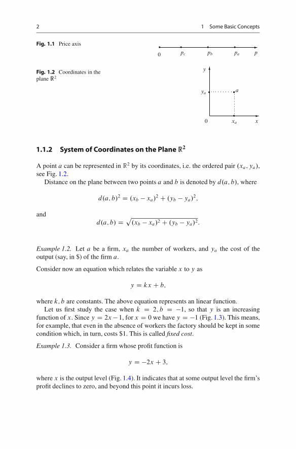
Fig. 1.1 Price axis �0 pc pb pa p� � � �
Fig. 1.2 Coordinates in theplane R2
�
�
0 xa x
ya
y
a
�
� �
1.1.2 System of Coordinates on the Plane R2
A point a can be represented in R2 by its coordinates, i.e. the ordered pair .xa; ya/,see Fig. 1.2.
Distance on the plane between two points a and b is denoted by d.a; b/, where
d.a; b/2 D .xb � xa/2 C .yb � ya/2;
andd.a; b/ D
p.xb � xa/2 C .yb � ya/2:
Example 1.2. Let a be a firm, xa the number of workers, and ya the cost of theoutput (say, in $) of the firm a.
Consider now an equation which relates the variable x to y as
y D kx C b;
where k; b are constants. The above equation represents an linear function.Let us first study the case when k D 2; b D �1, so that y is an increasing
function of x. Since y D 2x� 1, for x D 0 we have y D �1 (Fig. 1.3). This means,for example, that even in the absence of workers the factory should be kept in somecondition which, in turn, costs $1. This is called fixed cost.
Example 1.3. Consider a firm whose profit function is
y D �2x C 3;
where x is the output level (Fig. 1.4). It indicates that at some output level the firm’sprofit declines to zero, and beyond this point it incurs loss.

1.1 Introduction 3
Fig. 1.3 The linear costfunction: fixed cost case
�
�
�
�
x
y
y D 2x � 1
�
�����������
�����������
Fig. 1.4 The linear costfunction: the case of loss atsome output level
�
�
�
�
x
y
y D �2x C 3
�
����������
����������
Fig. 1.5 The linear demandfunction
�
�
p
qd
qd D a � bp
a
ab
��
��
�
��
��
�
Let us switch to a more realistic model. Consider a market with a single good,and assume that the quantity demanded qd is a decreasing function of the price p ofthe good, i.e.,
qd D a � bp;
where a; b > 0(Fig. 1.5).
4 1 Some Basic Concepts
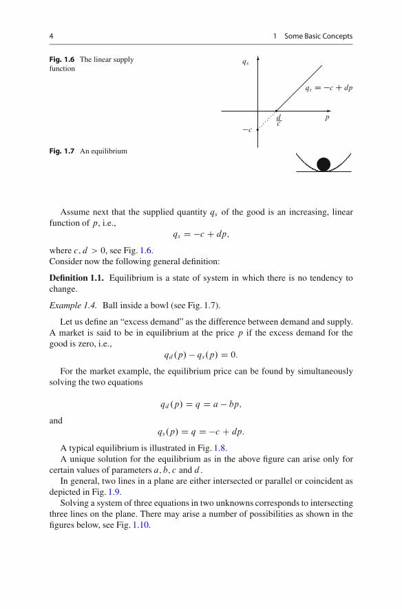
Fig. 1.6 The linear supplyfunction
�
�
p
qs
�c �
�
dc
qs D �c C dp
Fig. 1.7 An equilibrium
�
Assume next that the supplied quantity qs of the good is an increasing, linearfunction of p, i.e.,
qs D �c C dp;
where c; d > 0, see Fig. 1.6.Consider now the following general definition:
Definition 1.1. Equilibrium is a state of system in which there is no tendency tochange.
Example 1.4. Ball inside a bowl (see Fig. 1.7).
Let us define an “excess demand” as the difference between demand and supply.A market is said to be in equilibrium at the price p if the excess demand for thegood is zero, i.e.,
qd .p/� qs.p/ D 0:
For the market example, the equilibrium price can be found by simultaneouslysolving the two equations
qd .p/ D q D a � bp;
andqs.p/ D q D �c C dp:
A typical equilibrium is illustrated in Fig. 1.8.A unique solution for the equilibrium as in the above figure can arise only for
certain values of parameters a; b; c and d .In general, two lines in a plane are either intersected or parallel or coincident as
depicted in Fig. 1.9.Solving a system of three equations in two unknowns corresponds to intersecting
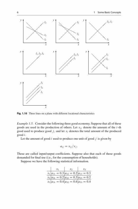
three lines on the plane. There may arise a number of possibilities as shown in thefigures below, see Fig. 1.10.

1.1 Introduction 5
�
�
�
�
qd ; qs
qd D a � bp
a
ab
��
��
�
��
��
�
�c
dc
q
p
�
qs D �c C dp
Fig. 1.8 The market equilibrium
�
�
x
y
��
��
�� l1
l2
�
�
x
y
l1
l2
�
�
x
y
l1; l2
Fig. 1.9 Two lines on a plane with different locational characteristics
In the first of the graphs in Fig. 1.10 three lines intersect at a unique point. In thesecond graph every pair of the three lines intersects at a unique point, giving threedistinct intersection points. In the third graph, the lines l2 and l3 coincide while theyintersect with l1 at a unique point. In the fourth graph all lines coincide. In the fifthgraph lines l2 and l3 coincide which are parallel to the separate line l1. In the nextgraph, the separate lines l2 and l3 are parallel to each other, intersecting with line l1at two distinct points. Finally, in the last graph the three separate lines are parallel.
Solving the system of three equations in three unknowns
8<
:
a11x1 C a12x2 C a13x3 D b1;
a21x1 C a22x2 C a23x3 D b2;
a31x1 C a32x2 C a33x3 D b3
is much more difficult than in the case of two equations with two unknowns.It is obvious that in the case of higher dimensions the number of possibilities is
enormously increasing, so that graphical tools then become almost inapplicable.Thus we need some analytical tools to solve and analyze arbitrarily large finitesystems of equations. To this end, in the following chapters we will deal with vectorsand matrices.
6 1 Some Basic Concepts
�
�
x
y
��
��
��
������
l1
l2
l3
�
�
x
y
��
��
��
������
l1
l2
l3
�
�
x
y
��
��
�� l1
l2; l3
�
�
x
y
l1; l2; l3
�
�
x
y
l2; l3
l1
�
�
x
y
�
��
��
l3
l2
l1
�
�
x
y
l3
l2
l1
Fig. 1.10 Three lines on a plane with different locational characteristics
Example 1.5. Consider the following three good economy. Suppose that all of thesegoods are used in the production of others. Let xij denote the amount of the i -thgood used to produce good j , and let xi denotes the total amount of the producedgood i .
Let the amount of good i used to produce one unit of good j is given by
aij D xij =xj :
These are called input/output coefficients. Suppose also that each of these goodsdemanded for final use (i.e., for the consumption of households).
Suppose we have the following statistical information.
x1 x2 x3
x1 a11 D 0:3 a12 D 0:2 a13 D 0:3
x2 a21 D 0:2 a22 D 0:3 a23 D 0:2
x3 a31 D 0:4 a32 D 0:6 a33 D 0:4
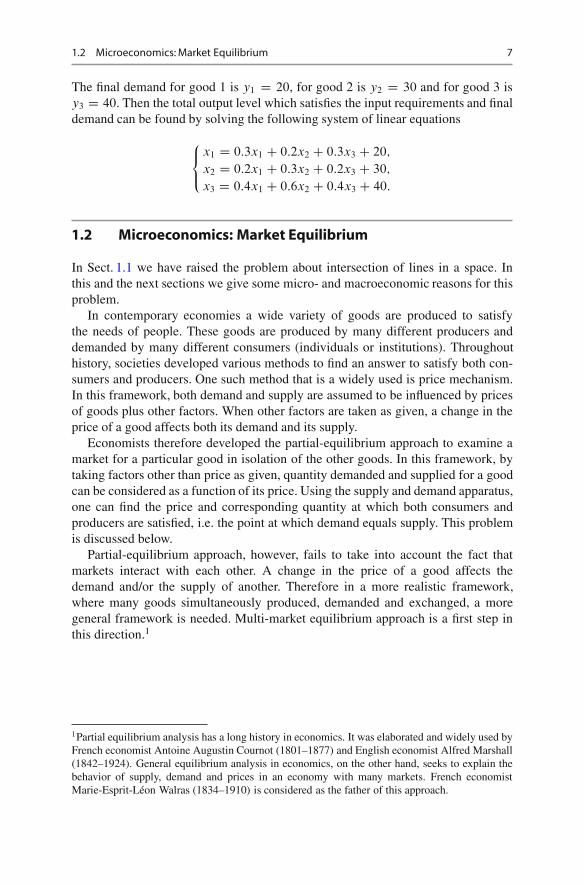
1.2 Microeconomics: Market Equilibrium 7
The final demand for good 1 is y1 D 20, for good 2 is y2 D 30 and for good 3 isy3 D 40. Then the total output level which satisfies the input requirements and finaldemand can be found by solving the following system of linear equations
8<
:
x1 D 0:3x1 C 0:2x2 C 0:3x3 C 20;
x2 D 0:2x1 C 0:3x2 C 0:2x3 C 30;
x3 D 0:4x1 C 0:6x2 C 0:4x3 C 40:
1.2 Microeconomics: Market Equilibrium
In Sect. 1.1 we have raised the problem about intersection of lines in a space. Inthis and the next sections we give some micro- and macroeconomic reasons for thisproblem.
In contemporary economies a wide variety of goods are produced to satisfythe needs of people. These goods are produced by many different producers anddemanded by many different consumers (individuals or institutions). Throughouthistory, societies developed various methods to find an answer to satisfy both con-sumers and producers. One such method that is a widely used is price mechanism.In this framework, both demand and supply are assumed to be influenced by pricesof goods plus other factors. When other factors are taken as given, a change in theprice of a good affects both its demand and its supply.
Economists therefore developed the partial-equilibrium approach to examine amarket for a particular good in isolation of the other goods. In this framework, bytaking factors other than price as given, quantity demanded and supplied for a goodcan be considered as a function of its price. Using the supply and demand apparatus,one can find the price and corresponding quantity at which both consumers andproducers are satisfied, i.e. the point at which demand equals supply. This problemis discussed below.
Partial-equilibrium approach, however, fails to take into account the fact thatmarkets interact with each other. A change in the price of a good affects thedemand and/or the supply of another. Therefore in a more realistic framework,where many goods simultaneously produced, demanded and exchanged, a moregeneral framework is needed. Multi-market equilibrium approach is a first step inthis direction.1
1Partial equilibrium analysis has a long history in economics. It was elaborated and widely used byFrench economist Antoine Augustin Cournot (1801–1877) and English economist Alfred Marshall(1842–1924). General equilibrium analysis in economics, on the other hand, seeks to explain thebehavior of supply, demand and prices in an economy with many markets. French economistMarie-Esprit-Leon Walras (1834–1910) is considered as the father of this approach.

8 1 Some Basic Concepts
1.2.1 Equilibrium in a Single Market
Let us consider an isolated market for good i . Suppose that both the demand (qdi )
and supply (qsi ) of this good is a function of its price (pi ), only.2
qdi D ˛0 � ˛1pi (1.1)
qsi D �ˇ0 C ˇ1pi (1.2)
These functions assume that there is a linear relation between the quantitydemanded (or supplied) and the price of the good i .
Remark 1.1. Although, in economics texts (1.1) and (1.2) are usually referred to aslinear demand and supply functions, from a strictly mathematical point of view, theyare not. They have an extra constant slope term. In mathematics linear functions witha constant slope are called affine functions. Notice that in the case of affine functions,when the explanatory variable (in this example price) in the equation is zero,explained variable (in this example quantity demanded or supplied, respectively)can take non-zero values. Linear function formulation, on the other hand, does notallow it.
Question 1.1. Why in economics affine functions are used in formulating demandand supply functions?
All of the coefficients in (1.1) and (1.2) are assumed to be positive. The negativesign in front of the slope coefficient in the demand function indicates that, as priceof the good increases, its demand declines. The reverse holds for the supply. Thenegative sign in front of the intercept term in the supply equation implies that supplywill become positive only after the price of the good in question is positive andsufficiently high.
The market for good i is said to be in ‘equilibrium’ when the demand for good iis equal to its supply, i.e.
qdi D qs
i (1.3)
Recall that the difference between demand and supply is called excess demand.Using this concept, market equilibrium can also be characterized as the point atwhich excess demand is zero, i.e.
E.pi/ D qdi � qs
i D 0 (1.4)
2This basic demand and supply model is, obviously, an oversimplification. In economics, bothdemand and supply of a good is treated as functions of many variables, including prices of othergoods, income etc. In the next section on multi-market equilibrium, prices of other goods will beallowed to influence supply and demand.

1.2 Microeconomics: Market Equilibrium 9
Suppose we want to find the equilibrium of the market described by (1.1), (1.3)or (1.1), (1.4). Such an equilibrium point can be characterized by two variables,equilibrium price and the quantity. An easy way to find this point, is to substi-tute (1.1) and (1.2) into (1.4), i.e.
E.pi / D .˛0 � ˛1pi / � .�ˇ0 C ˇ1pi / D 0;
from which the equilibrium price Op can be derived as
Opi D ˛0 C ˇ0
˛1 C ˇ1
(1.5)
Equilibrium quantity level, on the other hand, can be obtained by substitut-ing (1.5) either in (1.1) (or (1.2)), which gives
Oqi D ˛0ˇ1 � ˛1ˇ0
˛1 C ˇ1
(1.6)
Obviously, (1.6) gives an economically meaningful result, i.e. Oqi > 0 only if˛0ˇ1 � ˛1ˇ0 > 0.
Example 1.6. Letqd D 38� 2p
be the demand function andqs D �6C 9p
be the supply function for some good. Find the equilibrium price and correspondingquantity level.
Answer: Op D 4; Oq D 30.
1.2.2 Multi-Market Equilibrium
Consider an economy with two goods. Suppose that the supply and demand of eachgood are functions of its own price as well as the price of other good. Such a systemcan be represented by the following four equations:
qd1 D ˛01 C ˛11p1 C ˛12p2 (1.7)
qs1 D ˇ01 C ˇ11p1 C ˇ12p2 (1.8)
qd2 D ˛02 C ˛12p1 C ˛22p2 (1.9)
qs2 D ˇ02 C ˇ12p1 C ˇ22p2 (1.10)

10 1 Some Basic Concepts
For such economy, multi-market equilibrium is the quadruple . Op1; Op2; Oq1; Oq2/ atwhich
E1. Op1; Op2/ D qd1 . Op1; Op2/� qs
1. Op1; Op2/ D 0 (1.11)
andE2. Op1; Op2/ D qd
2 . Op1; Op2/� qs2. Op1; Op2/ D 0 (1.12)
are simultaneously satisfied.
Exercise 1.1. (i) Using (1.7)–(1.12) find the equilibrium prices for goods 1 and 2;(ii) what is the equilibrium quantity for good 1?
Hint. Use (1.11) and (1.12) to derive two equations with two unknowns (prices).Using one of the equations express one price in terms of the other. Substituting thisrelation in the other equation one gets an expression for one of the prices in termsof the parameters of the model. The expressions for other variables can be obtainedin a similar fashion through substitution.
Example 1.7. Consider an economy with two goods .q1; q2/. Let supply anddemand functions for these goods be as follows. For good 1:
qd1 D 3 � 2p1 C 2p2;
qs1 D �4C 3p1:
For good 2:qd
2 D 22C 2p1 � p2;
qs2 D 20C p2:
Find the equilibrium prices for goods 1 and 2.
Answer: p1 D 3; p2 D 4.
1.3 Macroeconomic Policy Problem
After the Second World War, governments’ role in management of the economywas widely accepted. The mode of government intervention varied from extensiveplanning both at macro and micro levels in socialist economies to the moremarket oriented monetary and fiscal policies adopted in advanced economies. Manydeveloping countries (such as India and Turkey) chose to implement developmentplanning which was less comprehensive than the socialist planning but still requiresmuch more intensive government intervention that the economic policies used inadvanced market economies.
As the commitment of the government became increasingly more extensive,it became necessary to have a framework to deal with them simultaneously andin a consistent manner. The seminal contribution in this field was made by Jan
1.3 Macroeconomic Policy Problem 11
Tinbergen3’s celebrated book, [31], which became the cornerstone of the theoryof economic policy since then.
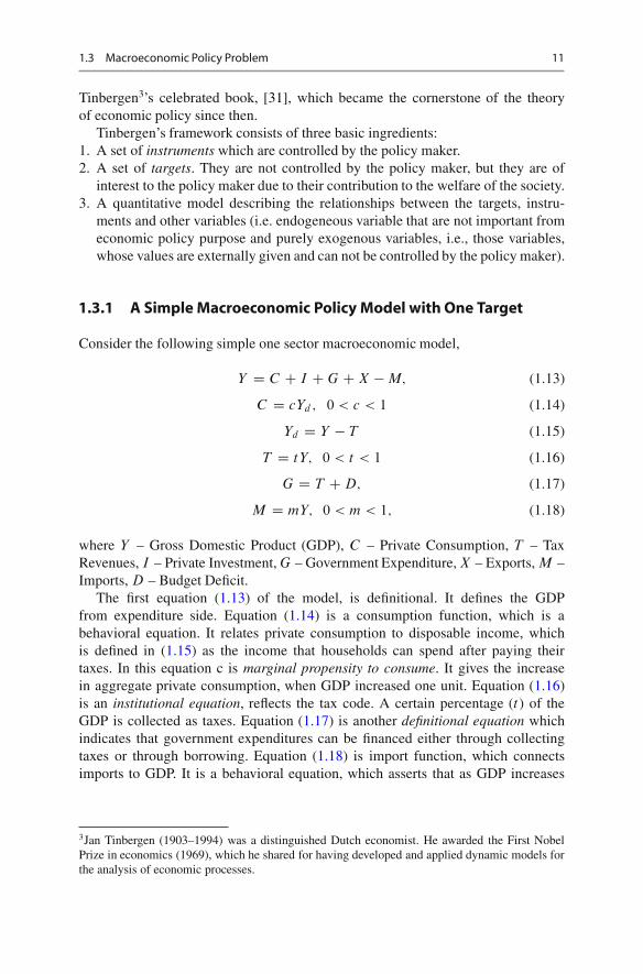
Tinbergen’s framework consists of three basic ingredients:1. A set of instruments which are controlled by the policy maker.2. A set of targets. They are not controlled by the policy maker, but they are of
interest to the policy maker due to their contribution to the welfare of the society.3. A quantitative model describing the relationships between the targets, instru-
ments and other variables (i.e. endogeneous variable that are not important fromeconomic policy purpose and purely exogenous variables, i.e., those variables,whose values are externally given and can not be controlled by the policy maker).
1.3.1 A Simple Macroeconomic Policy Model with One Target
Consider the following simple one sector macroeconomic model,
Y D C C I CG CX �M; (1.13)
C D cYd ; 0 < c < 1 (1.14)
Yd D Y � T (1.15)
T D tY; 0 < t < 1 (1.16)
G D T CD; (1.17)
M D mY; 0 < m < 1; (1.18)
where Y – Gross Domestic Product (GDP), C – Private Consumption, T – TaxRevenues, I – Private Investment, G – Government Expenditure, X – Exports, M –Imports, D – Budget Deficit.
The first equation (1.13) of the model, is definitional. It defines the GDPfrom expenditure side. Equation (1.14) is a consumption function, which is abehavioral equation. It relates private consumption to disposable income, whichis defined in (1.15) as the income that households can spend after paying theirtaxes. In this equation c is marginal propensity to consume. It gives the increasein aggregate private consumption, when GDP increased one unit. Equation (1.16)is an institutional equation, reflects the tax code. A certain percentage (t) of theGDP is collected as taxes. Equation (1.17) is another definitional equation whichindicates that government expenditures can be financed either through collectingtaxes or through borrowing. Equation (1.18) is import function, which connectsimports to GDP. It is a behavioral equation, which asserts that as GDP increases
3Jan Tinbergen (1903–1994) was a distinguished Dutch economist. He awarded the First NobelPrize in economics (1969), which he shared for having developed and applied dynamic models forthe analysis of economic processes.
12 1 Some Basic Concepts
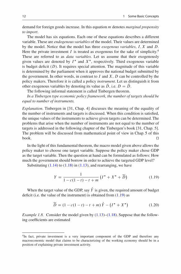
demand for foreign goods increase. In this equation m denotes marginal propensityto import.
The model has six equations. Each one of these equations describes a differentvariable. These are endogenous variables of the model. Their values are determinedby the model. Notice that the model has three exogenous variables, I; X and D.Here the private investment I is treated as exogenous for the sake of simplicity.4
These are referred to as data variables. Let us assume that their exogenouslygiven values are denoted by I � and X�, respectively. Third exogenous variableis budget deficit (D). It requires special attention. The magnitude of this variableis determined by the parliament when it approves the national budget submitted bythe government. In other words, in contrast to I and X , D can be controlled by thepolicy makers. Therefore it is called a policy instrument. Let us distinguish it fromother exogenous variables by denoting its value as QD, i.e. D D QD.
The following informal statement is called Tinbergen theorem.In a Tinbergen type economic policy framework, the number of targets should be
equal to number of instruments.
Explanation. Tinbergen in [31, Chap. 4] discusses the meaning of the equality ofthe number of instruments and targets is discussed. When this condition is satisfied,the unique values of the instruments to achieve given targets can be determined. Theproblems that arise when the number of instruments are not equal to the number oftargets is addressed in the following chapter of the Tinbergen’s book [31, Chap. 5].The problem will be discussed from mathematical point of view in Chap. 5 of thisbook. ut
In the light of this fundamental theorem, the macro model given above allows thepolicy maker to choose one target variable. Suppose the policy maker chose GDPas the target variable. Then the question at hand can be formulated as follows: Howmuch the government should borrow in order to achieve the targeted GDP level?
Substituting (1.14) to (1.18) in (1.13), and rearranging, we have
Y D 1
1� c.1 � t/ � t Cm
�I � CX� C eD
�(1.19)
When the target value of the GDP, say OY is given, the required amount of budgetdeficit (i.e. the value of the instrument) is obtained from (1.19) as
eD D .1 � c.1 � t/ � t Cm/ OY � �I � CX�� (1.20)
Example 1.8. Consider the model given by (1.13)–(1.18). Suppose that the follow-ing coefficients are estimated
4In fact, private investment is a very important component of the GDP and therefore anymacroeconomic model that claims to be characterizing of the working economy should be in aposition of explaining private investment activity.
1.3 Macroeconomic Policy Problem 13
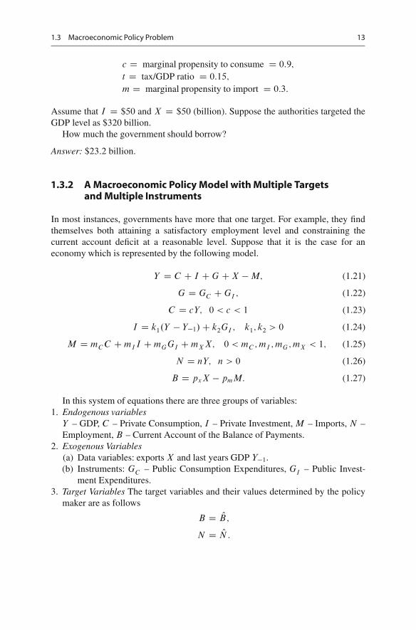
c D marginal propensity to consume D 0:9;
t D tax/GDP ratio D 0:15;
m D marginal propensity to import D 0:3:
Assume that I D $50 and X D $50 (billion). Suppose the authorities targeted theGDP level as $320 billion.
How much the government should borrow?
Answer: $23:2 billion.
1.3.2 A Macroeconomic Policy Model with Multiple Targetsand Multiple Instruments
In most instances, governments have more that one target. For example, they findthemselves both attaining a satisfactory employment level and constraining thecurrent account deficit at a reasonable level. Suppose that it is the case for aneconomy which is represented by the following model.
Y D C C I CG CX �M; (1.21)
G D GC CGI ; (1.22)
C D cY; 0 < c < 1 (1.23)
I D k1.Y � Y�1/C k2GI ; k1; k2 > 0 (1.24)
M D mC C CmI I CmGGI CmX X; 0 < mC ; mI ; mG; mX < 1; (1.25)
N D nY; n > 0 (1.26)
B D pxX � pmM: (1.27)
In this system of equations there are three groups of variables:1. Endogenous variables
Y – GDP, C – Private Consumption, I – Private Investment, M – Imports, N –Employment, B – Current Account of the Balance of Payments.
2. Exogenous Variables(a) Data variables: exports X and last years GDP Y�1.(b) Instruments: GC – Public Consumption Expenditures, GI – Public Invest-
ment Expenditures.3. Target Variables The target variables and their values determined by the policy
maker are as follows
B D OB;
N D ON :

14 1 Some Basic Concepts
The parameters are the following: c – share of consumption in income, t –average tax rate, m – import per unit of output, n – employment per unit of output(the reverse of productivity), px and pm – export and import prices, the coefficientk1 shows how much investment will be undertaken by the private agents in responseto an increase in GDP from its previous period level by unit, and k2 shows howmuch extra investment will be undertaken if government increases its investment byunit.
Example 1.9. Consider the model given by (1.21)–(1.27). Let
c D 0:8; k1 D 0:2; k2 D 0:05; mC D 0:1; mI D 0:4; mGD 0:3; mX D 0:2; n D 0:4:
SupposeY�1 D 100; X D 30:
Suppose also that the government wants to achieve the following targets
B D 0; N D 60:
Find the amounts of GC and GI .
Solution. We have the system of linear equations:
8ˆˆˆˆ<
ˆˆˆˆ:
Y D C C I CG C 30 �M;
G D GC CGI ;
C D 0:8Y;
I D 0:2.Y � 100/C 0:05GI ;
M D 0:1C C 0:4I C 0:3GI C 0:2 � 30;
60 D 0:4Y;
0 D px30 � pmM:
After the elimination of all variables but GI and GC , we obtain
GI D 93:75r � 68:75 and GC D 62:1875� 68:4375r;
where r D pX =pM .
Question 1.2. Explain and categorize equations (1.21)–(1.27) (definitional, techni-cal etc.)
Exercise 1.2. Find the values of the instruments that enable the system to achievethe targeted levels of current account balance and employment.

1.4 Problems 15
1.4 Problems
1. Plot each of the following pair of points on R2 and draw (and calculate thelength of) the line segment connecting them
(a) .4;�10/; .0; 1/; (b) .0; 0/; .�7;�8/; (c) .p
2;p
5/; .p
2;�p5/
2. Consider two points on x-axis. Show that the distance between them is equal tothe absolute value of the difference of their coordinates.
3. Draw the following lines in R2
(a) 3x � 4y D 12; (b) x C y D 10; (c) 2x � 5y D 10; (d) x D 5.
4. Write the equation of the lines determined by the two points in each part ofproblem 1.
5. Draw a line having (a) an x-intercept but no y-intercept, (b) a y-intercept butno x-intercept, (c) x-intercept and y-intercept as coincident.
6. Show that if a ¤ 0, b ¤ 0, then the intercepts of the line
ax C by C c D 0
are .0;�c=b/ and .�c=a; 0/.7. Show that
x
aC y
bD 1
is the equation of a straight line with the intercepts .0; b/ and .a; 0/.8. Solve 7x � 10 D 0 graphically by considering y D 7x � 10.9. Draw the lines for each of the following equations.
(a) jxj C jyj D 1; (b) jx C yj D 1.10. Solve the following systems of equations.
(a)
�3x � 5y D 15;
2x C y D 5I (b)
�3x � 5y D 15;
6x � 10y D 30I (c)
�6x � 10y D 30;
3x � 5y D 10:
11. Let �z1 D a11y1 C a12y2
z2 D a21y1 C a22y2
and �y1 D b11x1 C b12x2
y2 D b21x1 C b22x2:
Express z1 and z2 as functions of x1 and x2.

•

2Vectors and Matrices
2.1 Vectors
Ordered n-tuple of objects is called a vector
y D .y1; y2; : : : ; yn/:
Throughout the text we confine ourselves to vectors the elements yi of which arereal numbers.
In contrast, a variable the value of which is a single number, not a vector, is calledscalar.
Example 2.1. We can describe some economic unit EU by the vector
EU= (output, # of employees, capital stock, profit)
Given a vector y D .y1; : : : ; yn/, elements yi ; i D 1; : : : ; n are calledcomponents of the vector. We will usually denote vectors by bold letters.1 Thenumber n of components is called the dimension of the vector y. The set of alln–dimensional vectors is denoted by Rn and called n-dimensional real space2.
Two vectors x; y 2 Rn are equal if xi D yi for all i D 1; 2; : : : ; n.Let x D .x1; : : : ; xn/ and y D .y1; : : : ; yn/ be two vectors. We compare these
two vectors element by element and say that x is greater than y if for all i xi > yi ,and denote this statement by x > y. Analogously, we can define x � y.
Note that, unlike in the case of real numbers, for vectors when x > y does nothold, this does not imply y � x. Indeed, consider the vectors x D .1; 0/ and y D.0; 1/. It can be easily seen that neither x � y nor y � x is true.
1Some other notations for vectors are Ny and �!y .
2The terms arithmetic space, number space and coordinate space are also used.
F. Aleskerov et al., Linear Algebra for Economists, Springer Texts in Businessand Economics, DOI 10.1007/978-3-642-20570-5 2,© Springer-Verlag Berlin Heidelberg 2011
17

18 2 Vectors and Matrices
A vector 0 D .0; 0; : : : ; 0/ (also denoted by N0) is called a null vector.3
A vector x D .x1; x2; : : : ; xn/ is called non-negative (which is denoted by x � 0)if xi � 0 for all i .
A vector x is called positive if xi > 0 for all i . We denote this case by x > 0.
2.1.1 Algebraic Properties of Vectors
One can define the following natural arithmetic operations with vectors.Addition of two n-vectors
x C y D .x1 C y1; x2 C y2; : : : ; xn C yn/
Subtraction of two n-vectors
x � y D .x1 � y1; x2 � y2; : : : ; xn � yn/
Multiplication of a vector by a real number �
�y D .�y1; �y2; : : : ; �yn/
Example 2.2. Let EU1 D .Y1; L1; K1; P1/ be a vector representing an economicunit, say, a firm, see Example 2.1 (where, as usually, Y is its output, L is the numberof employees, K is the capital stock, and P is the profit). Let us assume that it ismerged with another firm represented by a vector EU2 D .Y2; L2; K2; P2/ (that is,we should consider two separate units as a single one). The resulting unit will berepresented by a sum of two vectors
EU3 D .Y1 C Y2; L1 C L2; K1 C K2; P1 C P2/ D EU1 C EU2:
In this situation, we have also EU2 D EU3 � EU1. Moreover, if the second firmis similar to the first one, we can assume that EU1 D EU2, hence the unit
EU3 D .2Y1; 2L1; 2K1; 2P1/ D 2 � EU1
gives also an example of the multiplication by a number 2.This example, as well as other ‘economic’ examples in this book has an
illustrative nature. Notice, however, that the profit of the merged firm might behigher or lower than the sum of two profits P1 C P2.
3The null vector is also called zero vector.

2.1 Vectors 19
The following properties of the vector operations above follow from the defini-tions:
1a. x C y D y C x (commutativity).1b. .x C y/ C z D x C .y C z/ (associativity).1c. x C 0 D x.1d. x C .�x/ D 0.2a. 1x D x.2b. �.�x/ D ��.x/.3a. .� C �/x D �x C �x.3b. �.x C y/ D �x C �y.
Exercise 2.1. Try to prove these properties yourself.
2.1.2 Geometric Interpretation of Vectors and Operationson Them
Consider R2 plane. Vector z D .˛1; ˛2/ is represented by a directed line segmentfrom the origin .0; 0/ to .˛1; ˛2/, see Fig. 2.1.
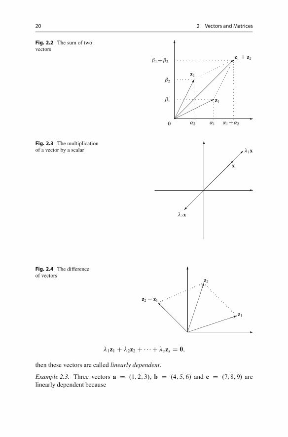
The sum of the two vectors z1 D .˛1; ˇ1/ and z2 D .˛2; ˇ2/ is obtained byadding up their coordinates, see Fig. 2.2.
In this figure, the sum z1 C z2 D .˛1 C˛2; ˇ1 Cˇ2/ is represented by a diagonalof a parallelogram sides of which being formed by the vectors z1 and z2.
Multiplication of a vector by a scalar has a contractionary (respectively, expan-sionary) effect if the scalar in absolute value is less (respectively, greater) than unity.The direction of the vector does not change if the scalar is positive, and it changesby 180 degrees if the scalar is negative. Figure 2.3 plots scalar multiplication for avector x, two scalars �1 > 1 and �1 < �2 < 0.
The difference of the two vectors z2 and z1 is shown on Fig. 2.4.The projection of the vector a on x�axis is denoted by prxa, and is shown in
Fig. 2.5 below.Let z1; : : : ; zs be a set of vectors in Rn. If there exist real numbers �1; : : : ; �s not
all being equal to 0 and
Fig. 2.1 A vector on theplane R2
�
�
�������
˛1
˛2 z D .˛1; ˛2/
0
20 2 Vectors and Matrices
Fig. 2.2 The sum of twovectors
�
�
�������
��
��
��
��
��
������
˛2 ˛1 ˛1 C˛2
ˇ1
ˇ2
ˇ1Cˇ2
z1
z2
z1 C z2
0
Fig. 2.3 The multiplicationof a vector by a scalar
�
�
��
��
���
��
����
��
�
�1x
x
�2x
Fig. 2.4 The differenceof vectors
�
�
���������
�
��
����
z2
z1
z2 � z1
�1z1 C �2z2 C � � � C �szs D 0;
then these vectors are called linearly dependent.
Example 2.3. Three vectors a D .1; 2; 3/, b D .4; 5; 6/ and c D .7; 8; 9/ arelinearly dependent because

2.1 Vectors 21
Fig. 2.5 The projectionof a vector a on the x-axis
�
�
��
���
�
a
prxa x
y
Fig. 2.6 Unit vectors in R3
x
y
z
e1=(1,0,0)e2=(0,1,0)
e3=(0,0,1)
1a � 2b C 1c D 0:
The vectors z1; : : : ; zs are called linearly independent if
�1z1 C � � � C �szs D 0
holds only whenever �1 D �2 D � � � D �s D 0.Note that the n vectors e1 D .1; 0; : : : ; 0/, e2 D .0; 1; : : : ; 0/, : : : , en D
.0; 0; : : : ; 1/ (see Fig. 2.6 for the case n D 3) are linearly independent in Rn.Assume that vectors z1; : : : ; zs are linearly dependent, i.e., there exists at least
one �i , where 1 � i � s, such that �i ¤ 0 and
�1z1 C �2z2 C � � � C �i zi C � � � C �szs D 0:
Then
�i zi D ��1z1 � �2z2 � � � � � �i�1zi�1 � �iC1ziC1 � � � � � �szs;
andzi D �1z1 C � � � C �i�1zi�1 C �iC1ziC1 C � � � C �szs; (2.1)
where �j D ��j =�i , for all j ¤ i and j 2 f1; : : : ; sg.
22 2 Vectors and Matrices
A vector a is called a linear combination of the vectors b1; : : : ; bn if it can berepresented as
a D ˛1b1 C � � � C ˛nbn;
where ˛1; : : : ; ˛n are real numbers. In particular, (2.1) shows that the vector zi is alinear combination of the vectors z1; : : : ; zi�1; ziC1; : : : ; zs .
These results can be formulated as
Theorem 2.1. If vectors z1; : : : ; zs are linearly dependent, then at least one ofthem is a linear combination of other vectors. Vectors one of which is a linearcombination of others are linearly dependent.
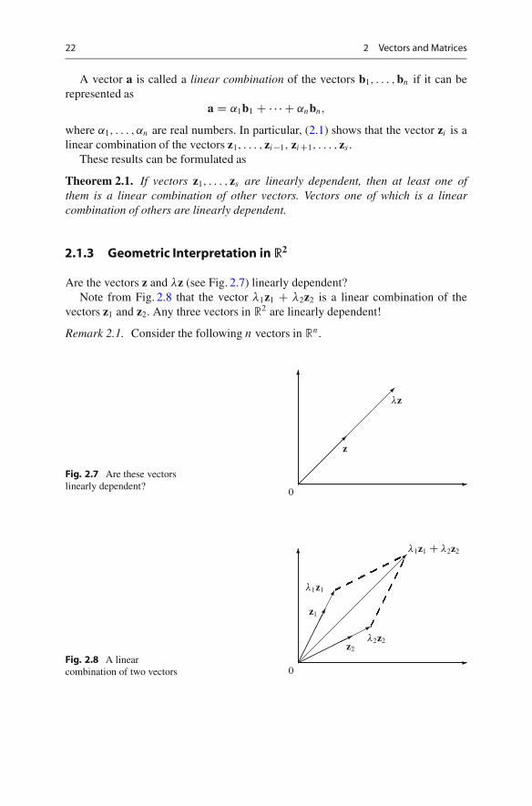
2.1.3 Geometric Interpretation in R2
Are the vectors z and �z (see Fig. 2.7) linearly dependent?Note from Fig. 2.8 that the vector �1z1 C �2z2 is a linear combination of the
vectors z1 and z2. Any three vectors in R2 are linearly dependent!
Remark 2.1. Consider the following n vectors in Rn.
Fig. 2.7 Are these vectorslinearly dependent? �
�
0�
��
��
��
��
��
���z
�z
Fig. 2.8 A linearcombination of two vectors
�
�
0������
�����
z1
�1z1
�������
������z2
�2z2
��
��
��
��
���1z1 C �2z2
2.2 Dot Product of Two Vectors 23
a1 D .1; �2; 0; 0; : : : ; 0/
a2 D .0; 1; �2; 0; : : : ; 0/
:: : ::: : ::: : :
an�1 D .0; 0; : : : ; 0; 1; �2/
an D .�2�.n�1/; 0; : : : ; 0; 0; 1/
These vectors are linearly dependent since
2�na1 C 2�.n�1/a2 C � � � C 2�1an D 0:
If n > 40 then 2�.n�1/ < 10�12, a very small number. Moreover, if n > 64, then2�n D 0 for computers. So, for n > 64, we can assume that in our system an isgiven by an D .0; : : : ; 0; 1/. Thus, the system is written as
8ˆˆˆˆ<
ˆˆˆˆ:
a1 D .1; �2; 0; 0; : : : ; 0/
a2 D .0; 1; �2; 0; : : : ; 0/
:: : :
:: : :
:: : :
an�1 D .0; 0; : : : ; 0; 1; �2/
an D .0; 0; : : : ; 0; 0; 1/
But this system is linearly independent. (Check it!)This example shows how sensitive might be linear dependency of vectors to
rounding.
Exercise 2.2. Check if the following three vectors are linearly dependent:(a) a D .1; 2; 1/; b D .�2; 3; �2/; c D .7; 4; 7/;(b) a D .1; 2; 3/; b D .0; �1; 3/; c D .2; �1; 2/.
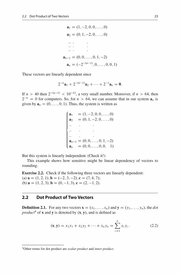
2.2 Dot Product of Two Vectors
Definition 2.1. For any two vectors x D .x1; : : : ; xn/ and y D .y1; : : : ; yn/, the dotproduct4 of x and y is denoted by .x; y/, and is defined as
.x; y/ D x1y1 C x2y2 C � � � C xnyn DnX
iD1
xi yi : (2.2)
4Other terms for dot product are scalar product and inner product.
24 2 Vectors and Matrices
Example 2.4. Let a1 D .1; �2; 0; : : : ; 0/ and a2 D .0; 1; �2; 0; : : : ; 0/. Then
.a1; a2/ D 1 � 0 C .�2/ � 1 C 0 � .�2/ C 0 � 0 C : : : C 0 � 0 D �2:
Example 2.5 (Household expenditures). Suppose the family consumes n goods. Letp be the vector of prices of these commodities (we assume competitive economy andtake them as given), and q be the vector of the amounts of commodities consumedby this household. Then the total expenditure of the household can be obtained bydot product of these two vectors
E D .p; q/:
Dot product .x; y/ of two vectors x and y is a real number and has the followingproperties, which can be checked directly:1. .x; y/ D .y; x/ (symmetry or commutativity)2. .�x; y/ D �.x; y/ for all � 2 R (associativity with respect to multiplication by a
scalar)3. .x1 C x2; y/ D .x1; y/ C .x2; y/ (distributivity)4. .x; x/ � 0 and .x; x/ D 0 iff x D 0 (non-negativity and non-degeneracy).
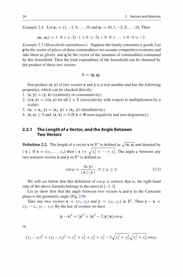
2.2.1 The Length of a Vector, and the Angle BetweenTwo Vectors
Definition 2.2. The length of a vector x in Rn is defined asp
.x; x/ and denoted by
j x j. If x D .x1; : : : ; xn/ then j x jDq
x21 C � � � C x2
n. The angle ' between anytwo nonzero vectors x and y in Rn is defined as
cos ' D .x; y/
j x j j y j ; 0 � ' � �: (2.3)
We will see below that this definition of cos ' is correct, that is, the right handside of the above formula belongs to the interval Œ�1; 1�.
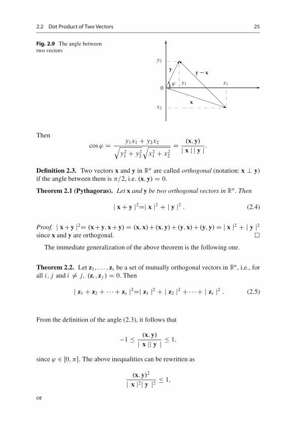
Let us show first that the angle between two vectors x and y in the Cartesianplane is the geometric angle (Fig. 2.9).
Take any two vectors x D .x1; x2/ and y D .y1; y2/ in R2. Then y � x D.y1 � x1; y2 � x2/. By the law of cosines we have
jy � xj2 D jyj2 C jxj2 � 2 jyj jxj cos ';
or
.y1 � x1/2 C .y2 � x2/2 D y21 C x2
1 C y22 C x2
2 � 2
qy2
1 C y22
qx2
1 C x22 cos ':
2.2 Dot Product of Two Vectors 25
Fig. 2.9 The angle betweentwo vectors
y2
y1
x2
x1 �
�
0 ����
������������
��
��
��
'
y
x
y � x
Then
cos ' D y1x1 C y2x2qy2
1 C y22
qx2
1 C x22
D .x; y/
j x j j y j :
Definition 2.3. Two vectors x and y in Rn are called orthogonal (notation: x ? y)if the angle between them is �=2, i.e. .x; y/ D 0.
Theorem 2.1 (Pythagoras). Let x and y be two orthogonal vectors in Rn. Then
j x C y j2Dj x j2 C j y j2 : (2.4)
Proof. j x Cy j2D .x Cy; x Cy/ D .x; x/C .x; y/C .y; x/C .y; y/ D j x j2 C j y j2since x and y are orthogonal. �
The immediate generalization of the above theorem is the following one.
Theorem 2.2. Let z1; : : : ; zs be a set of mutually orthogonal vectors in Rn, i.e., forall i; j and i ¤ j; .zi ; zj / D 0. Then
j z1 C z2 C � � � C zs j2Dj z1 j2 C j z2 j2 C � � � C j zs j2 : (2.5)
From the definition of the angle (2.3), it follows that
�1 � .x; y/
j x jj y j � 1;
since ' 2 Œ0; ��. The above inequalities can be rewritten as
.x; y/2
j x j2j y j2 � 1;
or
26 2 Vectors and Matrices
.x; y/2 � .x; x/ � .y; y/: (2.6)
The inequality (2.6) is called Cauchy5 inequality.Let us prove it so that we can better understand why the angle ' between two
vectors can take any value in the interval of Œ0; ��.
Proof. Given any two vectors x and y in Rn, consider the vector x � �y, where � isa real number. By axiom 4 of dot product we must have
.x � �y; x � �y/ � 0;
that is,�2.y; y/ � 2�.x; y/ C .x; x/ � 0:
But then the discriminant of the quadratic equation
�2.y; y/ � 2�.x; y/ C .x; x/ D 0
can not be positive. Therefore, it must be true that
.x; y/2 � .x; x/ � .y; y/ � 0:
�
Corollary 2.2. For all x and y in Rn,
j x C y j�j x j C j y j : (2.7)
Proof. Note that
j x C y j2D .x C y; x C y/ D .x; x/ C 2.x; y/ C .y; y/
Now using 2.x; y/ � 2 j .x; y/ j� 2 j x jj y j by Cauchy inequality, we obtain
j x C y j2 � .x; x/ C 2 j x j � j y j C .y; y/
D .j x j C j y j/2
implying the desired result. �
5Augustin Louis Cauchy (1789–1857) was a great French mathematician. In addition to his worksin algebra and determinants, he had created a modern approach to calculus, so-called epsilon–deltaformalism.
2.3 An Economic Example: Two Plants 27
Exercise 2.3. Plot the vectors u D .1; 2/, v D .�3; 1/ and their sum w D u C vand check visually the above inequality.
Exercise 2.4. Solve the system of equations
8<
:
.0; 0; 1; 1/ ? x;
.1; 2; 0; �1/ ? x;
hx; ai D jaj � jxj;
where a D .2; 1; 0; 0/ and x is an unknown vector from R4.
Exercise 2.5. Two vectors a and b are called parallel if they are linearly dependent(notation: akb). Solve the system of equations
�.0; 0; �3; 4/kx;
jxj D 15:
Exercise 2.6. Find the maximal angle of the triangle ABC , where A D .0; 1; 2; 0/,B D .0; 1; 0; �1/ and C D .1; 0; 0; 1/ are three points in R4.
Exercise 2.7. Given three points A.0; 1; 2; 3/, B.1; �1; 1; �1/ and C.1; 1; 0; 0/ inR4, find the length of the median AM of the triangle ABC .
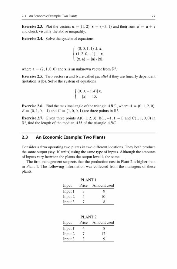
2.3 An Economic Example: Two Plants
Consider a firm operating two plants in two different locations. They both producethe same output (say, 10 units) using the same type of inputs. Although the amountsof inputs vary between the plants the output level is the same.
The firm management suspects that the production cost in Plant 2 is higher thanin Plant 1. The following information was collected from the managers of theseplants.
PLANT 1Input Price Amount used
Input 1 3 9Input 2 5 10Input 3 7 8
PLANT 2Input Price Amount used
Input 1 4 8Input 2 7 12Input 3 3 9

28 2 Vectors and Matrices
Question 1. Does this information confirm the suspicion of the firm management?
Answer. In order to answer this question one needs to calculate the cost function. Letwij denote the price of the i th input at the j th plant and xij denote the quantity of i thinput used in production j th plant (i D 1; 2; 3 and j D 1; 2). Suppose both of thesemagnitudes are perfectly divisible, therefore can be represented by real numbers.The cost of production can be calculated by multiplying the amount of each inputby its price and summing over all inputs.
This means price and quantity vectors (p and q) are defined on real space andinner product of these vectors are defined. In other words, both p and q are in thespace R3. The cost function in this case can be written as an inner product of priceand quantity vectors as
c D .w; q/; (2.8)
where c is the cost, a scalar. Using the data in the above tables cost of productioncan be calculated by using (2.8) as:
In Plant 1 the total cost is 133, which implies that unit cost is 13.3.In Plant 2, on the other hand, cost of production is 143, which gives unit cost as
14.3 which is higher than the first plant.That is, the suspicion is reasonable.
Question 2. The manager of the Plant 2 claims that the reason of the cost differencesis the higher input prices in her region than in the other. Is the available informationsupports her claim?
Answer. Let the input price vectors for Plant 1 and 2 be denoted as p1 and p2.Suppose that the latter is a multiple � of the former, i.e.,
p2 D �p1:
Since both vectors are in the space R3, length is defined for both. From the definitionof length one can obtain that
jp2j D �jp1j:In this case, however as can be seen from the tables this is not the case. Plant I enjoyslower prices for inputs 2 and 3, whereas Plant 2 enjoys lower price for input 3. Fora rough guess, one can still compare the lengths of the input price vectors which are
jp1j D 9:11; jp2j D 8:60;
which indicates that price data does not support the claim of the manager of thePlant 2. When examined more closely, one can see that the Plant 2 uses the mostexpensive input (input 2) intensely. In contrast, Plant 2 managed to save from usingthe most expensive input (in this case input 3). Therefore, the manager needs toexplain the reasons behind the choice mixture of inputs in her plant.
2.4 Another Economic Application: Index Numbers 29
2.4 Another Economic Application: Index Numbers
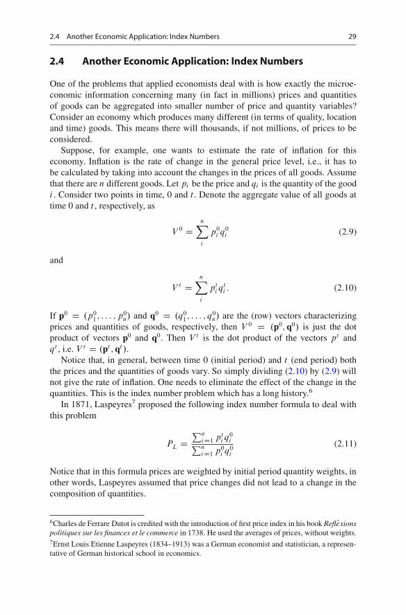
One of the problems that applied economists deal with is how exactly the microe-conomic information concerning many (in fact in millions) prices and quantitiesof goods can be aggregated into smaller number of price and quantity variables?Consider an economy which produces many different (in terms of quality, locationand time) goods. This means there will thousands, if not millions, of prices to beconsidered.
Suppose, for example, one wants to estimate the rate of inflation for thiseconomy. Inflation is the rate of change in the general price level, i.e., it has tobe calculated by taking into account the changes in the prices of all goods. Assumethat there are n different goods. Let pi be the price and qi is the quantity of the goodi . Consider two points in time, 0 and t . Denote the aggregate value of all goods attime 0 and t , respectively, as
V 0 DnX
i
p0i q0
i (2.9)
and
V t DnX
i
pti q
ti : (2.10)
If p0 D .p01; : : : ; p0
n/ and q0 D .q01 ; : : : ; q0
n/ are the (row) vectors characterizingprices and quantities of goods, respectively, then V 0 D .p0; q0/ is just the dotproduct of vectors p0 and q0. Then V t is the dot product of the vectors pt andqt , i.e. V t D .pt ; qt /.
Notice that, in general, between time 0 (initial period) and t (end period) boththe prices and the quantities of goods vary. So simply dividing (2.10) by (2.9) willnot give the rate of inflation. One needs to eliminate the effect of the change in thequantities. This is the index number problem which has a long history.6
In 1871, Laspeyres7 proposed the following index number formula to deal withthis problem
PL DPn
iD1 pti q
0iPn
iD1 p0i q0
i
(2.11)
Notice that in this formula prices are weighted by initial period quantity weights, inother words, Laspeyres assumed that price changes did not lead to a change in thecomposition of quantities.
6Charles de Ferrare Dutot is credited with the introduction of first price index in his book Refl Kexionspolitiques sur les finances et le commerce in 1738. He used the averages of prices, without weights.7Ernst Louis Etienne Laspeyres (1834–1913) was a German economist and statistician, a represen-tative of German historical school in economics.

30 2 Vectors and Matrices
In 1874, Paasche8, suggested using end-period weights, instead of the initialperiod’s
Pp DPn
iD1 pti q
tiPn
iD1 p0i qt
i
Laspeyeres index underestimates, whereas Paasche index overestimates the actualinflation.
Exercise 2.8. Formulate Laspeyres and Paasche indices in term of price andquantity vectors.
Outline of the answer:
PL D .pt ; q0/
.p0; q0/;
PP D .pt ; qt /
.p0; qt /:
Exercise 2.9. Consider a three good economy. The initial (t D 0) and end period’s(t D 1) prices and quantities of goods are as given in the following table:
Price (t D 0) Quantity (t D 0) Price (t D 1) Quantity (t D 1)
Good 1 2 50 1,8 90Good 2 1,5 90 2,2 70Good 3 0,8 130 1 100
i. Estimate the inflation (i.e. percentage change in overall price level) for thiseconomy by calculating Laspeyres index
ii. Repeat the same exercise by calculating Paasche index.
For further information on index numbers, we refer the reader to [9, 23].
2.5 Matrices
A matrix is a rectangular array of real numbers
2
666664
a11 a12 : : : a1n
a21 a22 : : : a2n
:: : : ::: : : ::: : : :
am1 am2 : : : amn
3
777775
:
8Hermann Paasche (1851–1925), German economist and statistician, was a professor of politicalscience at Aachen University.

2.5 Matrices 31
We will denote matrices with capital letters A,B,. . . The generic element of amatrix A is denoted by aij ; i D 1; : : : ; mI j D 1; : : : ; n, and the matrix itself isdenoted briefly as A D kaij km�n. Such a matrix with m rows and n columns is saidto be of order m � n If the matrix is square (that is, m D n), it is simply said to beof order n.
We denote by 0 the null matrix which contains zeros only. The identity matrixis a matrix I D In of size n � n whose elements are ik;k D 1 and ik;m D 0 fork ¤ m; k D 1; : : : ; n and m D 1; : : : ; n, that is, it has units on the diagonal andzeroes on the other places. The notion of the identity matrix will be discussed inSect. 3.2.
Example 2.6. Object – property: Consider m economic units each of which isdescribed by n indices. Units may be firms, and indices may involve the output,the number of employees, the capital stock, etc., of each firm.
Example 2.7. Consider an economy consisting of m D n sectors, where for alli; j 2 f1; 2; : : : ; ng, aij denotes the share of the output produced in sector i andused by sector j , in the total output of sector i . (Note that in this case the rowelements add up to one.)
Example 2.8. Consider m D n cities. Here aij is the distance between city i andcity j . Naturally, aii D 0, aij > 0, and aij D aj i for all i ¤ j , and i; j 2f1; 2; : : : ; ng.
We say that a matrix A D ��aij
��m�n
is non-negative if aij � 0 for all i D1; : : : ; mI j D 1; : : : ; n: This case is simply denoted by A � 0.
Analogously is defined a positive matrix A > 0.
2.5.1 Operations on Matrices
Let A D ��aij
��
m�nand B D �
�bij
��
m�nbe two matrices. The sum of these matrices
is defined asA C B D �
�aij C bij
��
m�n:
Example 2.9. 2
41 0
4 2
7 1
3
5C2
43 2
7 3
4 1
3
5 D2
44 2
11 5
11 2
3
5 :
Let A D ��aij
��
m�nand � 2 R. Then
�A D ���aij
��
m�n:

32 2 Vectors and Matrices
Example 2.10.
2
2
43 0
2 4
1 9
3
5 D2
46 0
4 8
2 18
3
5
Properties of Matrix Summation and Multiplication by a Scalar
(1-a) A C B D B C A.
(1-b) A C .B C C / D .A C B/ C C .
(1-c) A C .�A/ D 0, where �A D .�1/A.
(1-d) A C 0 D A.
(2-a) 1A D A.
(2-b) �.�A/ D .��/A; �; � 2 R.
(3-a) 0A D 0.
(3-b) .� C �/A D �A C �A; �; � 2 R.
(3-c) � .A C B/ D �A C �B; �; � 2 R.
The properties of these two operations are the same as for vectors from Rn. Wewill clarify this later in Chap. 6.
2.5.2 Matrix Multiplication
Let A D ��aij
��
m�nand B D �
�bjk
��
n�pbe two matrices. Then the matrix AB of
order m � p is defined as
AB D2
4nX
j D1
aij bjk
3
5
m�p
In other words, a product C D AB of the above matrices A and B is a matrixC D ��cij
��m�p
, where cij is equal to the dot product .Ai ; Bj / of the i -th row Ai of
the matrix A and the j -th column Bj of the matrix B considered as vectors from Rn.
Consider 2 � 2 case. Given
A D�
a11 a12
a21 a22
�and B D
�b11 b12
b21 b22
�;
2.5 Matrices 33
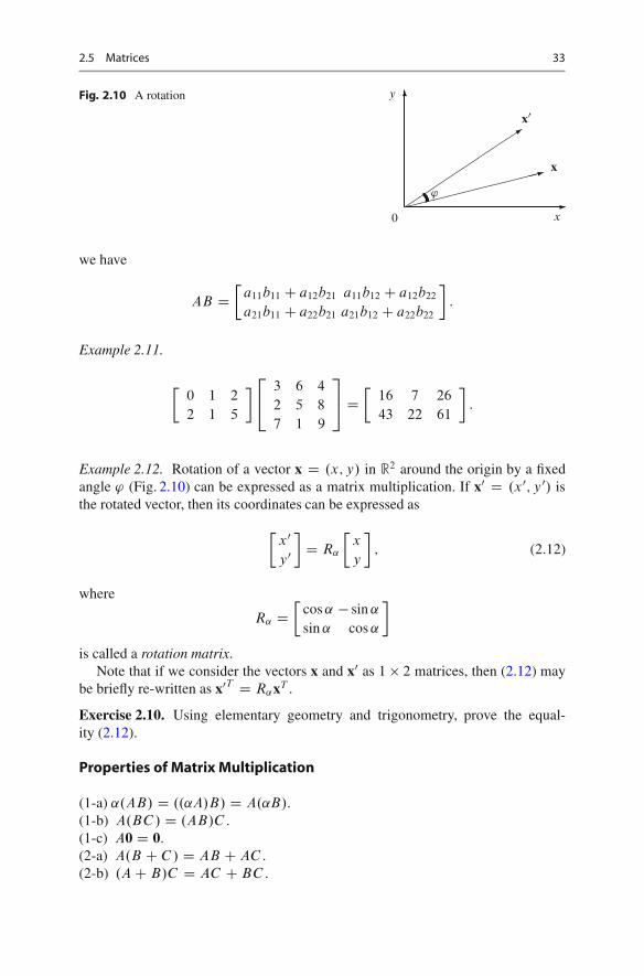
Fig. 2.10 A rotation
�
�
��
��
��
���
�����������
0
y
x
x0
x
'
we have
AB D�
a11b11 C a12b21 a11b12 C a12b22
a21b11 C a22b21 a21b12 C a22b22
�:
Example 2.11.
�0 1 2
2 1 5
�2
43 6 4
2 5 8
7 1 9
3
5 D�
16 7 26
43 22 61
�:
Example 2.12. Rotation of a vector x D .x; y/ in R2 around the origin by a fixedangle ' (Fig. 2.10) can be expressed as a matrix multiplication. If x0 D .x0; y0/ isthe rotated vector, then its coordinates can be expressed as
�x0y0�
D R˛
�x
y
�; (2.12)
where
R˛ D�
cos ˛ � sin ˛
sin ˛ cos ˛
�
is called a rotation matrix.Note that if we consider the vectors x and x0 as 1 � 2 matrices, then (2.12) may
be briefly re-written as x0T D R˛xT .
Exercise 2.10. Using elementary geometry and trigonometry, prove the equal-ity (2.12).
Properties of Matrix Multiplication
(1-a) ˛.AB/ D ..˛A/B/ D A.˛B/.(1-b) A.BC / D .AB/C .(1-c) A0 D 0.(2-a) A.B C C / D AB C AC .(2-b) .A C B/C D AC C BC .
34 2 Vectors and Matrices
Remark 2.2. Warning. AB ¤ BA, in general.
Indeed, let A and B be matrices of order m � n and n � p, respectively. Todefine the multiplication BA, we must have p D m. But matrices A and B may notcommute even if both of them are square matrices of order m � m. For example,consider
A D�
1 2
0 3
�and B D
��1 2
1 3
�:
We have
AB D�
1 8
3 9
�while BA D
��1 4
1 11
�:
Exercise 2.11. Let A and B be square matrices such that AB D BA. Show that:1. .A C B/2 D A2 C 2AB C B2.2. A2 � B2 D .A � B/.A C B/.
Exercise 2.12.� Prove the above properties of matrix multiplication.
Hint. To deduce the property 1-b), use the formulanP
iD1
mP
j D1
xij
!
DmP
j D1
�nP
iD1
xij
�.
Remark 2.3. The matrix multiplication defined above is one of the many conceptsthat are counted under the broader term “matrix product”. It is certainly the mostwidely used one. However, there are two other matrix products that are of someinterest to economists.
Kronecker Product of Matrices
Let A D kaij k be an m � n matrix and B D kbij k be a p � q matrix. Then theKronecker9 product of these two matrices is defined as
A ˝ B D2
4a11B : : : a1nB
: : : : : : : : :
am1B : : : amnB
3
5
which is an mp � nq matrix. Kronecker product is also referred to as direct productor tensor product of matrices. For its use in econometrics, see [1, 8, 14].
9Leopold Kronecker (1823–1891) was a German mathematician who made a great contributionboth to algebra and number theory. He was one of the founders of so-called constructivemathematics.
2.6 Transpose of a Matrix 35
Hadamard Product of Matrices
The Hadamard10 product of matrices (or elementwise product, or Shur11 product)of two matrices A D kaij k and B D kbij k of the same dimensions m � n is asubmatrix of the Kronecker product
A ı B D kaij bij km�n:
See [1, p. 340] and [24, Sect. 36] for the use of Hadamard product in matrixinequalities.
2.5.3 Trace of a Matrix
Given an n�n matrix A D kaij k, the sum of its diagonal elements Tr A D PniD1 ai i
is called the trace of the matrix A.
Example 2.13.
Tr
2
41 2 3
10 20 30
100 200 300
3
5 D 321
Exercise 2.13. Let A and B be two matrices of order n. Show that:
(a) Tr.A C B/ D Tr A C Tr B .(b)� Tr.AB/ D Tr.BA/.
2.6 Transpose of a Matrix
Let A D ��aij
��
m�n. The matrix B D �
�bij
��
n�mis called the transpose of A (and
denoted by AT ) if bij D aj i for all i 2 f1; 2; : : : ; mg and j 2 f1; 2; : : : ; ng.
Example 2.14.
2
43 0
2 4
1 9
3
5
T
D�
3 2 1
0 4 9
�
10Jacques Salomon Hadamard (1865–1963), a famous French mathematician who contributed inmany branches of mathematics such as number theory, geometry, algebra, calculus and dynamicalsystems, as well as in optics, mechanics and geodesy. His most popular book The psychology ofinvention in the mathematical field (1945) gives a nice description of mathematical thinking.11Issai Schur (1875–1941), an Israeli mathematician who was born in Belarus and died in Israel,made fundamental contributions to algebra, integral and algebraic equations, theory of matricesand number theory.
36 2 Vectors and Matrices
The transpose operator satisfies the following properties:1. .AT /T D A.2. .A C B/T D AT C BT .3. .˛A/T D ˛AT .4. .AB/T D BT AT .
Proof. To prove the above properties, note that one can formally write
AT D ��aij
��T
m�nD ��aj i
��n�m
:
Then .AT /T D ��aj i
��T
n�mD ��aij
��
m�nD A. This proves the property 1.
Now, .A C B/T D ��aij C bij
��T
m�nD �
�aj i C bj i
��
n�mD �
�aj i
��
n�mC�
�bj i
��
n�mD AT C BT . This gives the second property.
To check the third one, we deduce that .˛A/T D ��˛aij
��T
m�nD ��˛aj i
��T
n�mD
˛��aj i
��T
n�mD ˛AT .
Now, it remains to check the fourth property. Let M D AB and N D BT AT ,where the matrices A and B are of orders m � n and n� p, respectively. Then M D��˛mj i
��
m�pwith mij D .Ai ; Bj / and N D �
�˛nij
��
p�nwith nij D ..BT /i ; .AT /j /.
Since the transposition changes rows and columns, we have the equalities of vectors
.BT /i D Bi ; .AT /j D Aj :
Hence, mij D nj i for all i D 1; : : : ; m and j D 1; : : : ; p. Thus M T D N , asdesired. �
A matrix A is called symmetric if A D AT . A simple example of symmetricmatrices is the distance matrix A D Œaij �, where aij is the distance between thecities i and j . Obviously, aij D aj i or A D AT .
Theorem 2.3. For each matrix A of order n � n, the matrix AAT is symmetric.
Proof. Consider .AAT /T . By the properties 3) and 4), we have .AAT /T D.AT /T AT D AAT . �Exercise 2.14. Let A and B be two matrices of order n. Show that Tr AT D Tr A.
2.7 Rank of a Matrix
Are the vectors x; y, and z in the Fig. 2.11 linearly dependent?It is obvious that there exists � such that
u C �z D 0;
or˛x C ˇy C �z D 0;
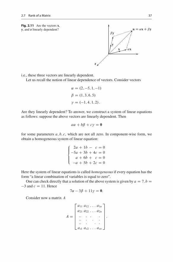
2.7 Rank of a Matrix 37
Fig. 2.11 Are the vectors x,y, and z linearly dependent?
�
�
������
���������������
��
��
��
��
�
˛x
ˇy
xy
z
u D ˛x C ˇy
i.e., these three vectors are linearly dependent.Let us recall the notion of linear dependence of vectors. Consider vectors
˛ D .2; �5; 1; �1/
ˇ D .1; 3; 6; 5/
� D .�1; 4; 1; 2/ :
Are they linearly dependent? To answer, we construct a system of linear equationsas follows: suppose the above vectors are linearly dependent. Then
a˛ C bˇ C c� D 0
for some parameters a; b; c, which are not all zero. In component-wise form, weobtain a homogeneous system of linear equation:
8ˆ<
ˆ:
2a C 1b � c D 0
�5a C 3b C 4c D 0
a C 6b C c D 0
�a C 5b C 2c D 0
Here the system of linear equations is called homogeneous if every equation has theform “a linear combination of variables is equal to zero”.
One can check directly that a solution of the above system is given by a D 7; b D�3 and c D 11. Hence
7˛ � 3ˇ C 11� D 0:
Consider now a matrix A
A D
2
666664
a11 a12 : : : a1n
a21 a22 : : : a2n
:: : : ::: : : ::: : : :
as1 as2 : : : asn
3
777775
:
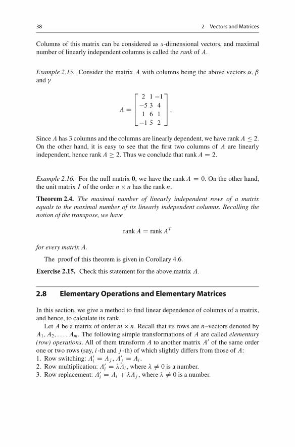
38 2 Vectors and Matrices
Columns of this matrix can be considered as s-dimensional vectors, and maximalnumber of linearly independent columns is called the rank of A.
Example 2.15. Consider the matrix A with columns being the above vectors ˛; ˇ
and �
A D
2
664
2 1 �1
�5 3 4
1 6 1
�1 5 2
3
775 :
Since A has 3 columns and the columns are linearly dependent, we have rank A � 2.On the other hand, it is easy to see that the first two columns of A are linearlyindependent, hence rank A � 2. Thus we conclude that rank A D 2.
Example 2.16. For the null matrix 0, we have the rank A D 0. On the other hand,the unit matrix I of the order n � n has the rank n.
Theorem 2.4. The maximal number of linearly independent rows of a matrixequals to the maximal number of its linearly independent columns. Recalling thenotion of the transpose, we have
rank A D rank AT
for every matrix A.
The proof of this theorem is given in Corollary 4.6.
Exercise 2.15. Check this statement for the above matrix A.
2.8 Elementary Operations and Elementary Matrices
In this section, we give a method to find linear dependence of columns of a matrix,and hence, to calculate its rank.
Let A be a matrix of order m � n. Recall that its rows are n–vectors denoted byA1; A2; : : : ; Am. The following simple transformations of A are called elementary(row) operations. All of them transform A to another matrix A0 of the same orderone or two rows (say, i -th and j -th) of which slightly differs from those of A:1. Row switching: A0
i D Aj , A0j D Ai .
2. Row multiplication: A0i D �Ai , where � ¤ 0 is a number.
3. Row replacement: A0i D Ai C �Aj , where � ¤ 0 is a number.
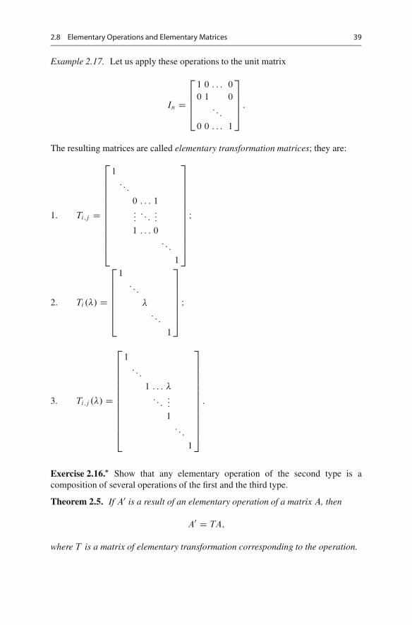
2.8 Elementary Operations and Elementary Matrices 39
Example 2.17. Let us apply these operations to the unit matrix
In D
2
6664
1 0 : : : 0
0 1 0: : :
0 0 : : : 1
3
7775
:
The resulting matrices are called elementary transformation matrices; they are:
1. Ti;j D
2
6666666666664
1
: : :
0 : : : 1:::
: : ::::
1 : : : 0: : :
1
3
7777777777775
I
2. Ti .�/ D
2
6666664
1: : :
�: : :
1
3
7777775
I
3. Ti;j .�/ D
2
6666666666664
1: : :
1 : : : �
: : ::::
1: : :
1
3
7777777777775
:
Exercise 2.16.� Show that any elementary operation of the second type is acomposition of several operations of the first and the third type.
Theorem 2.5. If A0 is a result of an elementary operation of a matrix A, then
A0 D TA;
where T is a matrix of elementary transformation corresponding to the operation.
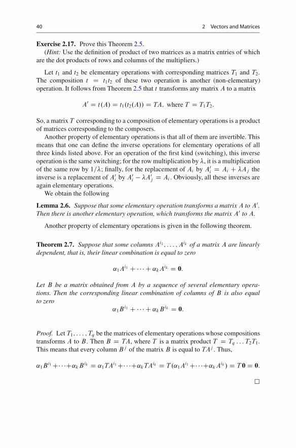
40 2 Vectors and Matrices
Exercise 2.17. Prove this Theorem 2.5.(Hint: Use the definition of product of two matrices as a matrix entries of which
are the dot products of rows and columns of the multipliers.)
Let t1 and t2 be elementary operations with corresponding matrices T1 and T2.The composition t D t1t2 of these two operation is another (non-elementary)operation. It follows from Theorem 2.5 that t transforms any matrix A to a matrix
A0 D t.A/ D t1.t2.A// D TA; where T D T1T2:
So, a matrix T corresponding to a composition of elementary operations is a productof matrices corresponding to the composers.
Another property of elementary operations is that all of them are invertible. Thismeans that one can define the inverse operations for elementary operations of allthree kinds listed above. For an operation of the first kind (switching), this inverseoperation is the same switching; for the row multiplication by �, it is a multiplicationof the same row by 1=�; finally, for the replacement of Ai by A0
i D Ai C �Aj theinverse is a replacement of A0
i by A0i � �A0
j D Ai . Obviously, all these inverses areagain elementary operations.
We obtain the following
Lemma 2.6. Suppose that some elementary operation transforms a matrix A to A0.Then there is another elementary operation, which transforms the matrix A0 to A.
Another property of elementary operations is given in the following theorem.
Theorem 2.7. Suppose that some columns Ai1; : : : ; Aik of a matrix A are linearlydependent, that is, their linear combination is equal to zero
˛1Ai1 C � � � C ˛kAik D 0:
Let B be a matrix obtained from A by a sequence of several elementary opera-tions. Then the corresponding linear combination of columns of B is also equalto zero
˛1Bi1 C � � � C ˛kBik D 0:
Proof. Let T1; : : : ; Tq be the matrices of elementary operations whose compositionstransforms A to B . Then B D TA, where T is a matrix product T D Tq : : : T2T1.This means that every column Bj of the matrix B is equal to TAj . Thus,
˛1Bi1 C� � �C˛kBik D ˛1TAi1 C� � �C˛kTAik D T .˛1Ai1 C� � �C˛kAik / D T 0 D 0:
�
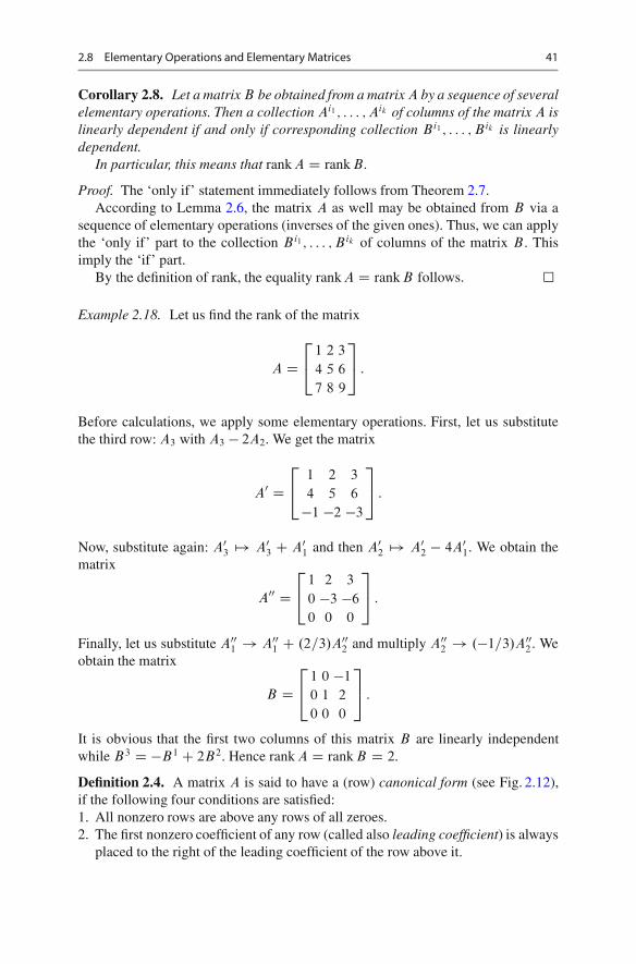
2.8 Elementary Operations and Elementary Matrices 41
Corollary 2.8. Let a matrix B be obtained from a matrix A by a sequence of severalelementary operations. Then a collection Ai1; : : : ; Aik of columns of the matrix A islinearly dependent if and only if corresponding collection Bi1; : : : ; Bik is linearlydependent.
In particular, this means that rank A D rank B .
Proof. The ‘only if’ statement immediately follows from Theorem 2.7.According to Lemma 2.6, the matrix A as well may be obtained from B via a
sequence of elementary operations (inverses of the given ones). Thus, we can applythe ‘only if’ part to the collection Bi1; : : : ; Bik of columns of the matrix B . Thisimply the ‘if’ part.
By the definition of rank, the equality rank A D rank B follows. �
Example 2.18. Let us find the rank of the matrix
A D2
41 2 3
4 5 6
7 8 9
3
5 :
Before calculations, we apply some elementary operations. First, let us substitutethe third row: A3 with A3 � 2A2. We get the matrix
A0 D2
41 2 3
4 5 6
�1 �2 �3
3
5 :
Now, substitute again: A03 7! A0
3 C A01 and then A0
2 7! A02 � 4A0
1. We obtain thematrix
A00 D2
41 2 3
0 �3 �6
0 0 0
3
5 :
Finally, let us substitute A001 ! A00
1 C .2=3/A002 and multiply A00
2 ! .�1=3/A002 . We
obtain the matrix
B D2
41 0 �1
0 1 2
0 0 0
3
5 :
It is obvious that the first two columns of this matrix B are linearly independentwhile B3 D �B1 C 2B2. Hence rank A D rank B D 2.
Definition 2.4. A matrix A is said to have a (row) canonical form (see Fig. 2.12),if the following four conditions are satisfied:1. All nonzero rows are above any rows of all zeroes.2. The first nonzero coefficient of any row (called also leading coefficient) is always
placed to the right of the leading coefficient of the row above it.

42 2 Vectors and Matrices
Fig. 2.12 Row echelon formof a matrix
*
*
* ** *
0
*
Fig. 2.13 Canonical form ofa matrix 1
**
0
*1
11
0 0 0*
3. All leading coefficients are equal to 1.4. All entries above a leading coefficient in the same column are equal to 0.
If only first two of the above conditions are satisfied, then the matrix is said tohave a row echelon form (see Fig. 2.13).
Example 2.19. In Example 2.18 above, the marix A00 has a row echelon form whilethe matrix B has even a canonical form.
It is easy to calculate the rank of a matrix in an echelon form: it is simply equalto the number of nonzero rows in it.
Theorem 2.9. Every matrix A can be transformed via a number of elementaryoperations to another matrix B in a row echelon form (and even in a canonicalform). Then the rank of the matrix A is equal to the number of nonzero rows of thematrix B .
Let us give an algorithm to construct an echelon form of the matrix. Thisalgorithm is called the Gaussian12 elimination procedure. It reduces all columnsof the matrix one-by-one to the columns of some matrix in a row echelon form. In arecent step, we assume that a submatrix consisting of the first .j � 1/ columns hasan echelon form. Suppose that this submatrix has .i � 1/ nonzero rows.
In the j -th step, we provide the following:1. If all elements of the j -th column beginning with aij and below are equal to zero,
the procedure is terminated. Then we go to the .j C 1/-th step of the algorithm.2. Otherwise, find the first nonzero element (say, aij ) in the j -th column in the i -th
row and below. If it is not aij , switch two rows Ai and Aj of the matrix. (seeFig. 2.14).
Now, we obtain a matrix A such that apk ¤ 0 (Fig. 2.15).
12Carl Friedrich Gauss (1777–1855) was a great German mathematician and physicist. He madefundamental contribution to a lot of branches of pure and applied mathematics including geodesy,statistics, and astronomy.

2.8 Elementary Operations and Elementary Matrices 43
Fig. 2.14 The Gaussianelimination, row switching
*
*
*
* *
*0
0
0 0
*
0 * * *
*
j
ak,j
ai,j
ak,j+1k
i
k+1
Fig. 2.15 The Gaussianelimination, row subtraction
*
*
*
* *
*0
0
ai,j+1
k
0 ai,j
* *
0
0
i
* * *
ak,j+1
j
-Ai*ak+1,j/ai,jk+1
Fig. 2.16 The Gaussianelimination, the result of rowsubtractions
*
*
*
* *
*
0
0
* *
ak,j+10
* *0
j
ai,j ai,j+1
0
k
i
k+1
3. For every p > i , provide the following row replacement: the row Ap ! Ap �.apj =aij /Aj (Fig. 2.16).These three types of operations are sufficient to construct a row echelon form. In
the next step of the algorithm, we take p C 1 in place of p and j C 1 in place of j .Note that in the above Example 2.18 we used this algorithm to transform A0 to
A00. Another example is given below.
Example 2.20. Using Gauss algorithm, let us construct a row echelon form of thematrix
A D2
40 0 3
2 6 �2
4 12 �1
3
5 :
In the beginning, i D j D 1, that is, we begin with the first column. In operation1, we find the first nonzero element of this column, that is, a21. In operation 2, weswitch the first and the second rows and get the matrix
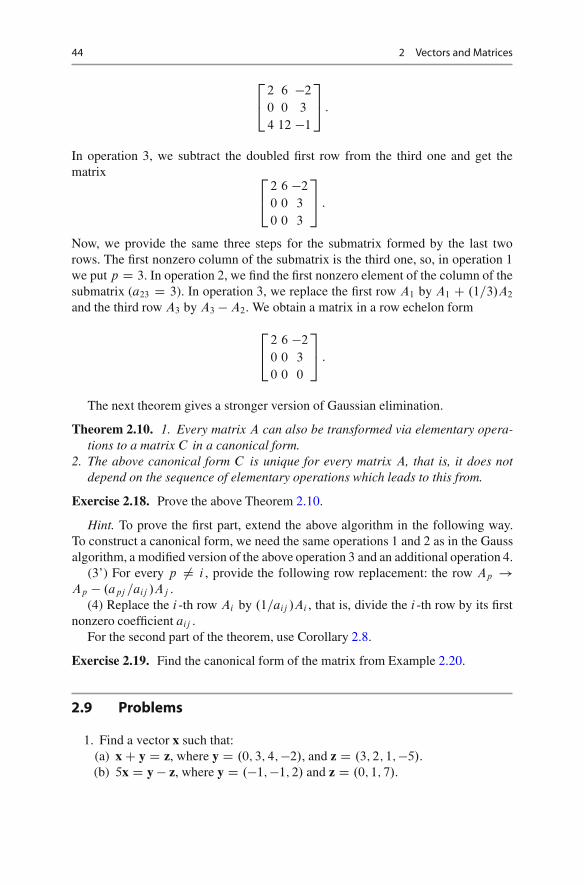
44 2 Vectors and Matrices
2
42 6 �2
0 0 3
4 12 �1
3
5 :
In operation 3, we subtract the doubled first row from the third one and get thematrix 2
42 6 �2
0 0 3
0 0 3
3
5 :
Now, we provide the same three steps for the submatrix formed by the last tworows. The first nonzero column of the submatrix is the third one, so, in operation 1we put p D 3. In operation 2, we find the first nonzero element of the column of thesubmatrix (a23 D 3). In operation 3, we replace the first row A1 by A1 C .1=3/A2
and the third row A3 by A3 � A2. We obtain a matrix in a row echelon form
2
42 6 �2
0 0 3
0 0 0
3
5 :
The next theorem gives a stronger version of Gaussian elimination.
Theorem 2.10. 1. Every matrix A can also be transformed via elementary opera-tions to a matrix C in a canonical form.
2. The above canonical form C is unique for every matrix A, that is, it does notdepend on the sequence of elementary operations which leads to this from.
Exercise 2.18. Prove the above Theorem 2.10.
Hint. To prove the first part, extend the above algorithm in the following way.To construct a canonical form, we need the same operations 1 and 2 as in the Gaussalgorithm, a modified version of the above operation 3 and an additional operation 4.
(3’) For every p ¤ i , provide the following row replacement: the row Ap !Ap � .apj =aij /Aj .
(4) Replace the i -th row Ai by .1=aij /Ai , that is, divide the i -th row by its firstnonzero coefficient aij .
For the second part of the theorem, use Corollary 2.8.
Exercise 2.19. Find the canonical form of the matrix from Example 2.20.
2.9 Problems
1. Find a vector x such that:(a) x C y D z, where y D .0; 3; 4; �2/, and z D .3; 2; 1; �5/.(b) 5x D y � z, where y D .�1; �1; 2/ and z D .0; 1; 7/.
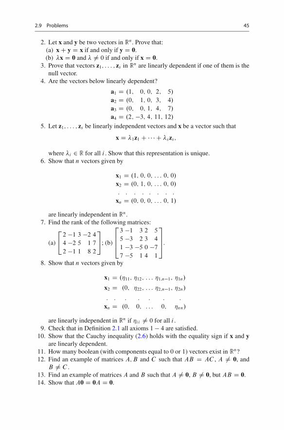
2.9 Problems 45
2. Let x and y be two vectors in Rn. Prove that:(a) x C y D x if and only if y D 0.(b) �x D 0 and � ¤ 0 if and only if x D 0.
3. Prove that vectors z1; : : : ; zs in Rn are linearly dependent if one of them is thenull vector.
4. Are the vectors below linearly dependent?
a1 D .1; 0; 0; 2; 5/
a2 D .0; 1; 0; 3; 4/
a3 D .0; 0; 1; 4; 7/
a4 D .2; �3; 4; 11; 12/
5. Let z1; : : : ; zs be linearly independent vectors and x be a vector such that
x D �1z1 C � � � C �szs;
where �i 2 R for all i . Show that this representation is unique.6. Show that n vectors given by
x1 D .1; 0; 0; : : : 0; 0/
x2 D .0; 1; 0; : : : 0; 0/
: : : : : : : :
xn D .0; 0; 0; : : : 0; 1/
are linearly independent in Rn.7. Find the rank of the following matrices:
(a)
2
42 �1 3 �2 4
4 �2 5 1 7
2 �1 1 8 2
3
5; (b)
2
664
3 �1 3 2 5
5 �3 2 3 4
1 �3 �5 0 �7
7 �5 1 4 1
3
775.
8. Show that n vectors given by
x1 D .�11; �12; : : : �1;n�1; �1n/
x2 D .0; �22; : : : �2;n�1; �2n/
: : : : : : :
xn D .0; 0; : : : 0; �nn/
are linearly independent in Rn if �ii ¤ 0 for all i .9. Check that in Definition 2.1 all axioms 1 � 4 are satisfied.
10. Show that the Cauchy inequality (2.6) holds with the equality sign if x and yare linearly dependent.
11. How many boolean (with components equal to 0 or 1) vectors exist in Rn?12. Find an example of matrices A; B and C such that AB D AC , A ¤ 0, and
B ¤ C .13. Find an example of matrices A and B such that A ¤ 0, B ¤ 0, but AB D 0.14. Show that A0 D 0A D 0.

46 2 Vectors and Matrices
15. Prove that .˛A/.ˇB/ D .˛ˇ/ AB for all real numbers ˛ and ˇ, and for allmatrices A and B such that the matrix products exist.
16. Prove that .˛A/ B D ˛ .AB/ D A .˛B/ for each real number ˛ and for allmatrices A and B such that the matrix products exist.
17. Let A; B and C be n � n matrices. Show that ABC D CAB if AC D CA andBC D CB .
18. Find a 2 � 3 matrix A and a 3 � 2 matrix B such that
AB D�
1 0
0 1
�:
19. Let
A D�
1 �1
�3 3
�:
(a) Find x ¤ 0 such that Ax D 0.(b) Find y ¤ 0 such that yA D 0.
20. Let ˛ and ˇ be two angles. Prove the following property of rotation matrices:
R˛Cˇ D R˛Rˇ:
21. Prove the properties of matrix summation.22. Calculate
2
40 2 �1
�2 �1 2
3 �2 �1
3
5
2
470 34 �107
52 26 �68
101 50 �140
3
5
2
427 �18 10
�46 31 �17
3 2 1
3
5 :
23. How A � B will change if:(a) i th and j th rows of A are interchanged?(b) a constant c times j th row of A is added to its i th row?
(c) i th and j th columns of B are interchanged?
(d) a constant c times j th column of B is added to its i th column?24.* Show that rank.AB/ � rank A and rank.AB/ � rank B .25.* Show that the sum of the entries of the Hadamard product AıB of two matrices
A and B of order n (so-called a Frobenius13 product) .A; B/F is equal toTr ABT .
26.* Prove that any matrix A can be represented as A D B C C , where B issymmetric matrix and C is an anti-symmetric matrix (i.e., C T D �C ).
27. Find all 2 � 2 matrices A satisfying A2 D 0.28. Find all 2 � 2 matrices A satisfying A2 D I2.
13Ferdinand Georg Frobenius (1849–1917) was a famous German algebraist. He made a greatcontribution to group theory and also proved a number of significant theorems in algebraicequations, geometry, number theory, and theory of matrices.

2.9 Problems 47
29. Find a row echelon form and the rank of the matrix
2
40 0 �1 3
�2 �1 2 1
2 1 �4 5
3
5 :
30. Find the canonical form of the matrix
2
41 3 0 0
5 15 2 1
�2 �6 1 3
3
5 :

•
3Square Matrices and Determinants
The following section illustrates how a matrix can be used to represent a system oflinear equations.
3.1 Transformation of Coordinates
Let our ‘old’ coordinate system be .x; y/, and ‘new’ coordinate system be .x0; y0/,see Fig. 3.1.
It is obvious that this transformation from .x; y/ to .x0; y0/ consists of twomoves: translation and rotation. Note that a translation after rotation also yields thesame transformation. Let us study these two moves separately.
3.1.1 Translation
We move the origin O D .0; 0/ to O 0 D .x0; y0/, without changing the direction ofaxes (Fig. 3.2). Then each point X with coordinates .�; �/ with respect to the firstsystem get the coordinates .�; �/ with respect to the second system, where
��0 D � � x0;
�0 D � � y0:
In the vector form, the above system can be re-written as an equality
.� 0; �0/ D .�; �/ � .x0; y0/:
After a translation has been made, rotation is applied.
F. Aleskerov et al., Linear Algebra for Economists, Springer Texts in Businessand Economics, DOI 10.1007/978-3-642-20570-5 3,© Springer-Verlag Berlin Heidelberg 2011
49

50 3 Square Matrices and Determinants
Fig. 3.1 Two coordinatesystems in a plane
�
�
��
��
���
��
��
���
x
y
0
00
y0 x0
Fig. 3.2 The translation
�
�
�
�
0
y
�
y0
x0 � x
y0
�0
00 �0 x0
Fig. 3.3 The rotation
�
�
����������
�
00
y0
�0
�0 x0
��
���
y00
�00�00
x00
˛
˛
3.1.2 Rotation
We rotate the system by an angle ˛ around O 0 (Fig. 3.3). Then the point X withthe coordinates .� 0; �0/ (with respect to the old coordinate system) get the newcoordinates .� 00; �00/, where
�� 00 D � 0 cos ˛ C �0 sin ˛;
�00 D �� 0 sin ˛ C �0 cos ˛:
In matrix notation the above system can be rewritten as
�cos ˛ sin ˛
� sin ˛ cos ˛
� ��0�0�D�
� 00�00�
:

3.2 Square Matrices 51
Note that here the matrix
R�˛ D�
cos ˛ sin ˛
� sin ˛ cos ˛
�
is the matrix of rotation by the opposite angle �˛, see Example 2.12.Then the general transformation can be written as
�� 00 D .� � x0/ cos ˛ C .�� y0/ sin ˛;
�00 D �.� � x0/ sin ˛ C .� � y0/ cos ˛;
or �� 00�00�D R�˛
���
�
���
x0
y0
��:
3.2 Square Matrices
3.2.1 Identity Matrix
As a very special matrix form, we can define the identity matrix, which will be usedin many matrix operations. In fact, we already defined the identity matrix but nowwe do it in general form. Before that, let us first introduce Kronecker delta functionto be
ıij D�
1; if i D j;
0; otherwise.
Identity matrix can, then, be defined as
In D��ıij
��
n�n
or
In D
2
664
1 0 : : : : : : 0
0 1 : : : : : : 0
: : : : : : : : : : : : : : : :
0 0 : : : : : : 1
3
775 :
Lemma 3.1. Let A D ��aij
��
n�n, then AIn D InA D A:
Proof. Consider AIn DhPn
j D1 aij ıjk
i
n�n. If j ¤ k then ıjk D 0 and aij ıjk D 0;
if j D k then ıjk D 1 and aij ıjj D aij : Analogously can be proved InA D A. �
52 3 Square Matrices and Determinants
3.2.2 Power of a Matrix and Polynomial of a Matrix
Let A be a square matrix of order m. We can define the power of any square matrixA in the following way
A0 D In
A1 D A
A2 D AA
: : : : : : : : : :
An D A � An�1
Usual polynomial is given by f .x/ D anxn C an�1xn�1 C � � � C a1x C a0. Thepolynomial of the matrix A can be similarly defined as
f .A/ D anAn C an�1An�1 C � � � C a1AC a0Im:
Example 3.1. Let
A D�
2 3
1 0
�
and f .x/ D x2 � 2x � 1. Then
f .A/ D A2 � 2A� I2 D�
7 6
2 3
���
4 6
2 0
���
1 0
0 1
�D�
2 0
0 2
�:
3.3 Systems of Linear Equations: The Case of Two Variables
Consider an arbitrary system of two linear equations in two variables
�a11x1 C a12x2 D b1
a21x1 C a22x2 D b2
(3.1)
For the above system, let
A D�
a11 a12
a21 a22
�
2�2
be the matrix of the known coefficients,
x D�
x1
x2
�
2�1
be the vector of unknown variables, and

3.4 Determinant of a Matrix 53
b D�
b1
b2
�
2�1
be the vector of constants. Hence in the matrix form, we can rewrite our system oflinear equations as
Ax D b: (3.2)
Now, let us try to solve the above system (3.1) in the ‘generic’ case provided thatno division by zero will appear in our calculations. We will solve it by the exclusionof unknown variables.
Divide the first rows by a11 and the second row by a21 (we assume here that boththese numbers are non-zero!).
(x1 C .a12=a11/ x2 D b1=a11
x1 C .a22=a21/ x2 D b2=a21
Subtract the second row from the first one.�
a12
a11
� a22
a21
�x2 D b1
a11
� b2
a21
Then x2 is obtained as
x2 D .b1=a11/ � .b2=a21/
.a12=a11/ � .a22=a21/
D b2a11 � b1a21
a11a22 � a12a21
: (3.3)
(We again assume that the denominator a11a22 � a12a21 is non-zero!)Inserting the value of x2 into one of the original equations, and solving for x1, weget
x1 D b1a22 � b2a12
a11a22 � a12a21
: (3.4)
3.4 Determinant of a Matrix
For the coefficient matrix
A D�
a11 a12
a21 a22
�
let us define the function
det A D a11a22 � a21a12
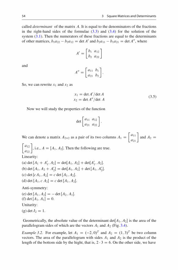
54 3 Square Matrices and Determinants
called determinant of the matrix A. It is equal to the denominators of the fractionsin the right-hand sides of the formulae (3.3) and (3.4) for the solution of thesystem (3.1). Then the numerators of these fractions are equal to the determinantsof other matrices, b1a22 � b2a12 D det A0 and b2a11 � b1a21 D det A00, where
A0 D�
b1 a12
b2 a22
�
and
A00 D�
a11 b1
a21 b2
�:
So, we can rewrite x1 and x2 as
x1 D det A0=det A
x2 D det A00=det A(3.5)
Now we will study the properties of the function
det
�a11 a12
a21 a22
�:
We can denote a matrix A2�2 as a pair of its two columns A1 D�
a11
a21
�and A2 D
�a12
a22
�, i.e., A D ŒA1; A2�. Then the following are true.
Linearity:
(a) det ŒA1 C A01; A2� D detŒA1; A2�C detŒA0
1; A2�.
(b) det ŒA1; A2 C A02� D detŒA1; A2�C det ŒA1; A0
2�.
(c) det ŒcA1; A2� D c det ŒA1; A2�.
(d) det ŒA1; c A2� D c det ŒA1; A2�.
Anti-symmetry:
(e) det ŒA1; A2� D � det ŒA2; A1�.(f) det ŒA1; A1� D 0.
Unitarity:
(g) det I2 D 1.
Geometrically, the absolute value of the determinant detŒA1; A2� is the area of theparallelogram sides of which are the vectors A1 and A2 (Fig. 3.4).
Example 3.2. For example, let A1 D .�2; 0/T and A2 D .1; 3/T be two columnvectors. The area of the parallelogram with sides A1 and A2 is the product of thelength of the bottom side by the hight, that is, 2 � 3 D 6. On the other side, we have

3.4 Determinant of a Matrix 55
Fig. 3.4 The area of thisparallelogram is jdet[A1 , A2]j
0������
A1
������A2
�
detŒA1; A2� D det
��2 0
1 3
�D �6;
a number with the same absolute value.
The determinant of an n � n matrix is defined as follows.
Definition 3.1. Let A D Œaij �n�n. The minor Mij of A is the determinant of thematrix formed from A by removing the i -th row and the j -th column; the productAij D .�1/iCj Mij is called a cofactor of the element aij .
Then in terms of row i elements and the respective cofactors, the determinant ofA is
det A DnX
j D1
aij Aij (3.6)
or in terms of column j elements and their cofactors, it is
det A DnX
iD1
aij Aij : (3.7)
One could prove1 that all these formulae for different i give the same numberdet A.
Example 3.3. Let
A D2
41 2 3
5 0 6
7 8 9
3
5 :
Using the decomposition by, say, the second row (the relation (3.6) with i D 2), wehave
1See, e. g., [33, Theorem 2.4.5].
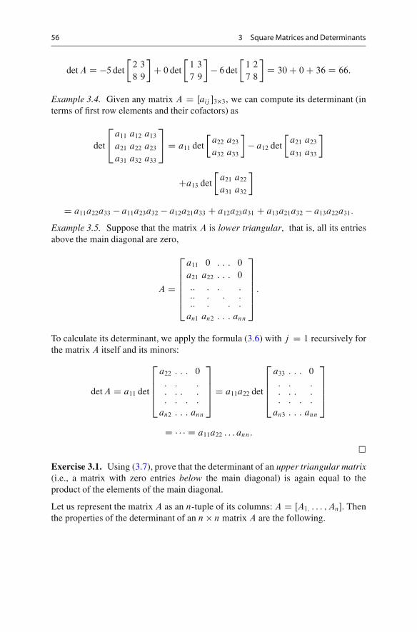
56 3 Square Matrices and Determinants
det A D �5 det
�2 3
8 9
�C 0 det
�1 3
7 9
�� 6 det
�1 2
7 8
�D 30C 0C 36 D 66:
Example 3.4. Given any matrix A D Œaij �3�3, we can compute its determinant (interms of first row elements and their cofactors) as
det
2
4a11 a12 a13
a21 a22 a23
a31 a32 a33
3
5 D a11 det
�a22 a23
a32 a33
�� a12 det
�a21 a23
a31 a33
�
Ca13 det
�a21 a22
a31 a32
�
D a11a22a33 � a11a23a32 � a12a21a33 C a12a23a31 C a13a21a32 � a13a22a31:
Example 3.5. Suppose that the matrix A is lower triangular, that is, all its entriesabove the main diagonal are zero,
A D
2
666664
a11 0 : : : 0
a21 a22 : : : 0
:: : : ::: : : ::: : : :
an1 an2 : : : ann
3
777775
:
To calculate its determinant, we apply the formula (3.6) with j D 1 recursively forthe matrix A itself and its minors:
det A D a11 det
2
6664
a22 : : : 0
: : :: : : :: : : :
an2 : : : ann
3
7775D a11a22 det
2
6664
a33 : : : 0
: : :: : : :: : : :
an3 : : : ann
3
7775
D � � � D a11a22 : : : ann:
�
Exercise 3.1. Using (3.7), prove that the determinant of an upper triangular matrix(i.e., a matrix with zero entries below the main diagonal) is again equal to theproduct of the elements of the main diagonal.
Let us represent the matrix A as an n-tuple of its columns: A D ŒA1; : : : ; An�. Thenthe properties of the determinant of an n � n matrix A are the following.

3.4 Determinant of a Matrix 57
3.4.1 The Basic Properties of Determinants
Linearity:
.a/ det ŒA1; : : : ; Ai�1; Ai C A0i ; AiC1; : : : ; An� D
det ŒA1; : : : ; Ai�1; Ai ; AiC1; : : : ; An�C detŒA1; : : : ; Ai�1; A0i ; AiC1; : : : ; An�
.b/ det ŒA1; : : : ; Ai�1; cAi ; AiC1; : : : ; An�Dc det ŒA1; : : : ; Ai�1; Ai ; AiC1; : : : ; An�
Anti-symmetry:
.c/ det ŒA1; : : : ; Ai ; : : : ; Aj ; : : : ; An� D � det ŒA1; : : : ; Aj ; : : : ; Ai ; : : : ; An�
That is, switching the i -th and j -th columns of a matrix changes the sign of itsdeterminant.
Unitarity:
.d/ det In D 1
Many other properties of determinants (including the formulae (3.6) and (3.7) fromthe definition) can be deduced from the above basic properties (a)–(d). For example,one can obtain
Corollary 3.1. The following properties of determinants are also hold:
.e/ det ŒA1; : : : ; Ai�1; B; AiC1; : : : ; Aj �1; B; Aj C1; : : : ; An� D 0
.f / det ŒA1; : : : ; Ai�1; Ai C cAj ; AiC1; : : : ; An� D detŒA1; : : : ; An�
.g/ det ŒA1; : : : ; Ai�1; 0; AiC1; : : : ; An� D 0
Proof. .e/ Let A be the matrix ŒA1; : : : ; Ai�1; B; AiC1; : : :; Aj �1; B; Aj C1; : : :; An�.According to the anti-symmetry property .e/ above, we have
det A D � det A;
hence det A D 0..f / Now, let A D ŒA1; : : : ; Ai�1; Ai C cAj ; AiC1; : : : ; An�. By the property .a/,
we have
det AD detŒA1; : : :; Ai�1; Ai ; AiC1; : : :; An�CdetŒA1; : : :; Ai�1; cAj ; AiC1; : : :; An�:
By the properties .b/ and .e/, the second component in the sum here is equal to
detŒA1; : : : ; Ai�1; cAj ; AiC1; : : : ; Aj ; : : : ; An�
D c detŒA1; : : : ; Ai�1; Aj ; AiC1; : : : ; Aj ; : : : ; An� D c � 0 D 0;
hence det A D detŒA1; : : : ; An�.
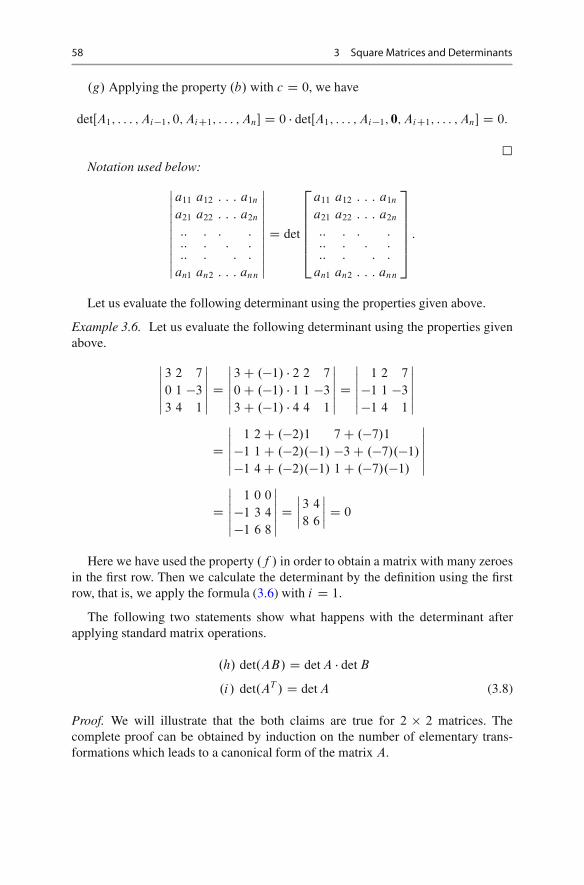
58 3 Square Matrices and Determinants
.g/ Applying the property .b/ with c D 0, we have
detŒA1; : : : ; Ai�1; 0; AiC1; : : : ; An� D 0 � detŒA1; : : : ; Ai�1; 0; AiC1; : : : ; An� D 0:
�Notation used below:
ˇˇˇˇˇˇˇˇˇ
a11 a12 : : : a1n
a21 a22 : : : a2n
:: : : ::: : : ::: : : :
an1 an2 : : : ann
ˇˇˇˇˇˇˇˇˇ
D det
2
666664
a11 a12 : : : a1n
a21 a22 : : : a2n
:: : : ::: : : ::: : : :
an1 an2 : : : ann
3
777775
:
Let us evaluate the following determinant using the properties given above.
Example 3.6. Let us evaluate the following determinant using the properties givenabove.
ˇˇˇˇˇ
3 2 7
0 1 �3
3 4 1
ˇˇˇˇˇDˇˇˇˇˇ
3C .�1/ � 2 2 7
0C .�1/ � 1 1 �3
3C .�1/ � 4 4 1
ˇˇˇˇˇDˇˇˇˇˇ
1 2 7
�1 1 �3
�1 4 1
ˇˇˇˇˇ
Dˇˇˇˇˇ
1 2C .�2/1 7C .�7/1
�1 1C .�2/.�1/ �3C .�7/.�1/
�1 4C .�2/.�1/ 1C .�7/.�1/
ˇˇˇˇˇ
Dˇˇˇˇˇ
1 0 0
�1 3 4
�1 6 8
ˇˇˇˇˇDˇˇˇˇ3 4
8 6
ˇˇˇˇ D 0
Here we have used the property .f / in order to obtain a matrix with many zeroesin the first row. Then we calculate the determinant by the definition using the firstrow, that is, we apply the formula (3.6) with i D 1.
The following two statements show what happens with the determinant afterapplying standard matrix operations.
.h/ det.AB/ D det A � det B
.i/ det.AT / D det A (3.8)
Proof. We will illustrate that the both claims are true for 2 � 2 matrices. Thecomplete proof can be obtained by induction on the number of elementary trans-formations which leads to a canonical form of the matrix A.

3.4 Determinant of a Matrix 59
(h) Let
A D�
a11 a12
a21 a22
�and B D
�b11 b12
b21 b22
�:
Then
AB D�
a11b11 C a12b21 a11b12 C a12b22
a21b11 C a22b21 a21b12 C a22b22
�
and
det.AB/ Dˇˇˇa11b11 a11b12
a21b11 a21b12
ˇˇˇC
ˇˇˇa12b21 a11b12
a22b21 a21b12
ˇˇˇ
Cˇˇˇa11b11 a12b22
a21b11 a22b22
ˇˇˇC
ˇˇˇa12b21 a12b22
a22b21 a22b22
ˇˇˇ
D b11b12
ˇˇˇa11 a11
a21 a21
ˇˇˇ� b21b12
ˇˇˇa11 a11
a21 a21
ˇˇˇC b11b22
ˇˇˇa11 a11
a21 a21
ˇˇˇ
Cb21b22
ˇˇˇa12 a12
a22 a22
ˇˇˇ
D .det A/ .b11b22 � b21b12/
D det A det B:
(i) Again, let
A D�
a11 a12
a21 a22
�:
Then
AT D�
a11 a21
a12 a22
�;
so that det AT D a11a22 � a21a12 D det A:
For the complete proof see, e.g., [33, Sect. 2.4]. �
Warning. If A is an n�n matrix and c is a real number, then det.cA/ D cn det A,not c det A!
The property .i/ implies that in the above properties .a/–.g/ one can replace thecolumns of the matrix A by the columns of its transpose AT , that is, rows of A. Weget
Corollary 3.2. All the above properties .a/–.g/ of determinants remains true afterreplacing the columns A1; : : : ; An of the matrix A by its rows.

60 3 Square Matrices and Determinants
3.4.2 Determinant and Elementary Operations
Recall that there are three type of simplest operations under the rows of matricescalled elementary operations, see Sect. 2.8, “Elementary operations and elementarymatrices”.
Proposition 3.1. If a square matrix A is transformed to another matrix A0 via anelementary operation e, then
det A0 D q det A;
where (according to the type of e) the number q is1. �1, if e is a row switching;2. �, if e is a row multiplication by a number �;3. 1, if e is a row replacement.
Proof. By Corollary 3.2, we may apply the properties .a/–.g/ of determinants tothe rows of the matrix A.1. By the anti-symmetry property .e/, the row switching multiplies the determinant
by �1.2. By the linearity property .b/, we have det A0 D � det A, hence q D �.3. By the linearity .f /, we have in this case det A0 D det A, i.e., q D 1.
�The above properties .a/–.g/ and Proposition 3.1 allows to evaluate determinants
of arbitrary high order.
Example 3.7. Let us evaluate the determinant of the matrix
A D
2
666666664
0 1 1 : : : 1 1
1 1 1 : : : 1 1
1 0 1 : : : 1 1:::
::::::
::::::
:::
1 0 0 : : : 1 1
1 0 0 : : : 0 1
3
777777775
of order n. Let us first apply to A elementary operations of the following kind: foreach i D 2; : : : ; n, replace i th row Ai by Ai � A1. Then
det A D
ˇˇˇˇˇˇˇˇˇˇˇˇ
0 1 1 : : : 1 1
1 0 0 : : : 0 0
1 �1 0 : : : 0 0:::
::::::
::::::
:::
1 �1 �1 : : : 0 0
1 �1 �1 : : : �1 0
ˇˇˇˇˇˇˇˇˇˇˇˇ
:
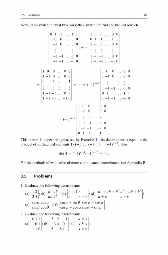
3.5 Problems 61
Now, let us switch the first two rows; then switch the 2nd and the 3rd row, etc.
ˇˇˇˇˇˇˇˇˇˇˇ
0 1 1 : : : 1 1
1 0 0 : : : 0 0
1 �1 0 : : : 0 0:::
::::::
::::::
:::
1 �1 �1 : : : 0 0
1 �1 �1 : : : �1 0
ˇˇˇˇˇˇˇˇˇˇˇ
D �
ˇˇˇˇˇˇˇˇˇˇˇ
1 0 0 : : : 0 0
0 1 1 : : : 1 1
1 �1 0 : : : 0 0:::
::::::
::::::
:::
1 �1 �1 : : : 0 0
1 �1 �1 : : : �1 0
ˇˇˇˇˇˇˇˇˇˇˇ
D
ˇˇˇˇˇˇˇˇˇˇˇˇ
1 0 0 : : : 0 0
1 �1 0 : : : 0 0
0 1 1 : : : 1 1:::
::::::
::::::
:::
1 �1 �1 : : : 0 0
1 �1 �1 : : : �1 0
ˇˇˇˇˇˇˇˇˇˇˇˇ
D � � � D .�1/n�2
ˇˇˇˇˇˇˇˇˇˇˇˇ
1 0 0 : : : 0 0
1 �1 0 : : : 0 0:::
::::::
::::::
:::
1 �1 �1 : : : 0 0
0 1 1 : : : 1 1
1 �1 �1 : : : �1 0
ˇˇˇˇˇˇˇˇˇˇˇˇ
D .�1/n�1
ˇˇˇˇˇˇˇˇˇˇˇˇ
1 0 0 : : : 0 0
1 �1 0 : : : 0 0:::
::::::
::::::
:::
1 �1 �1 : : : 0 0
1 �1 �1 : : : �1 0
0 1 1 : : : 1 1
ˇˇˇˇˇˇˇˇˇˇˇˇ
:
This matrix is upper triangular, so, by Exercise 3.1 its determinant is equal to theproduct of its diagonal elements 1 � .�1/ : : : .�1/ � 1 D .�1/n�2. Thus
det A D .�1/n�1.�1/n�2 D �1:
For the methods of evaluation of more complicated determinants, see Appendix B.
3.5 Problems
1. Evaluate the following determinants.
(a)
ˇˇˇ 1 2
3 4
ˇˇˇ; (b)
ˇˇˇa
2 ab
ab b2
ˇˇˇ; (c)
ˇˇˇnC 1 n
n n � 1
ˇˇˇ; (d)
ˇˇˇa
2 C ab C b2 a2 � ab C b2
aC b a � b
ˇˇˇ;
(e)
ˇˇˇˇsin ˛ cos ˛
sin ˇ cos ˇ
ˇˇˇˇ ; (f)
ˇˇˇˇsin ˛ C sin ˇ cos ˇ C cos ˛
cos ˇ � cos ˛ sin ˛ � sin ˇ
ˇˇˇˇ :
2. Evaluate the following determinants.
(a)
ˇˇˇˇˇ
0 1 1
1 0 1
1 1 0
ˇˇˇˇˇ; (b)
ˇˇˇˇˇ
7 2 �1
�3 4 0
5 �8 1
ˇˇˇˇˇ; (c)
ˇˇˇˇˇ
a x x
x b x
x x c
ˇˇˇˇˇ;

62 3 Square Matrices and Determinants
(d)
ˇˇˇˇˇ
˛2 C 1 ˛ˇ ˛�
˛ˇ ˇ2 C 1 ˇ�
˛� ˇ� �2 C 1
ˇˇˇˇˇ; (e)
ˇˇˇˇˇ
sin ˛ cos ˛ 1
sin ˇ cos ˇ 1
sin � cos � 1
ˇˇˇˇˇ.
3. Consider a transformation of coordinates in the plane which translate the originto the point .2;�3/ and then rotates the coordinate system by angle �=4. Give amatrix formula for the new coordinates .x0; y0/ of a point X in terms of its oldcoordinates .x; y/.
4. Evaluate the polynomial f .x/ D x3 � 7x2 C 13x � 5 of the matrix
A D2
45 2 �3
1 3 �1
2 2 �1
3
5 :
5. Let A be an arbitrary square matrix of order two, and let f .x/ be a polynomialx2 � ax C b, where a D Tr A and b D det A. Show that f .A/ D 0.
6. Prove thatˇˇˇˇˇˇ
0 1 1 a
1 0 1 b
1 1 0 c
a b c d
ˇˇˇˇˇˇD a2 C b2 C c2 � 2ab � 2bc � 2ac C 2d:
7. Evaluate the determinant ˇˇˇˇˇˇˇˇˇ
1 2 3 4 5
2 3 4 5 1
3 4 5 1 2
4 5 1 2 3
5 1 2 3 4
ˇˇˇˇˇˇˇˇˇ
:
8. Given a number d D det.A1; : : : ; An/, find det.An; : : : ; A1/.
9. Evaluate the following determinants of matrices of order n.
(a)
ˇˇˇˇˇˇˇˇˇˇ
1 1 1 : : : 1 1
1 1 1 : : : 1 0
1 1 1 : : : 0 0
� � � � � �1 1 0 : : : 0 0
1 0 0 : : : 0 0
ˇˇˇˇˇˇˇˇˇˇ
; (b)
ˇˇˇˇˇˇˇˇ
2 1 : : : 1
1 2 : : : 1:::
:::: : :
:::
1 1 : : : 2
ˇˇˇˇˇˇˇˇ
; (c)
ˇˇˇˇˇˇˇˇˇ
1 2 0 : : : 0 0
0 1 2 : : : 0 0:::
::::::
: : ::::
:::
0 0 0 : : : 1 2
2 0 0 : : : 0 1
ˇˇˇˇˇˇˇˇˇ
.
10. Suppose X is a matrix such that
X CX2 D �In:
Find det X .
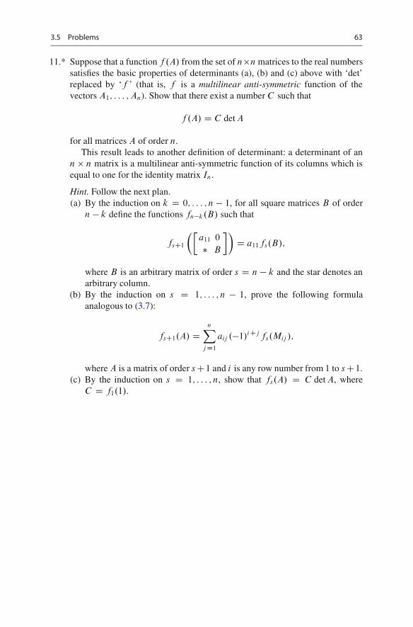
3.5 Problems 63
11.* Suppose that a function f .A/ from the set of n�n matrices to the real numberssatisfies the basic properties of determinants (a), (b) and (c) above with ‘det’replaced by ‘f ’ (that is, f is a multilinear anti-symmetric function of thevectors A1; : : : ; An). Show that there exist a number C such that
f .A/ D C det A
for all matrices A of order n.This result leads to another definition of determinant: a determinant of an
n � n matrix is a multilinear anti-symmetric function of its columns which isequal to one for the identity matrix In.
Hint. Follow the next plan.(a) By the induction on k D 0; : : : ; n � 1, for all square matrices B of order
n � k define the functions fn�k.B/ such that
fsC1
��a11 0
� B
��D a11fs.B/;
where B is an arbitrary matrix of order s D n � k and the star denotes anarbitrary column.
(b) By the induction on s D 1; : : : ; n � 1, prove the following formulaanalogous to (3.7):
fsC1.A/ DnX
j D1
aij .�1/iCj fs.Mij /;
where A is a matrix of order sC1 and i is any row number from 1 to sC1.(c) By the induction on s D 1; : : : ; n, show that fs.A/ D C det A, where
C D f1.1/.

•
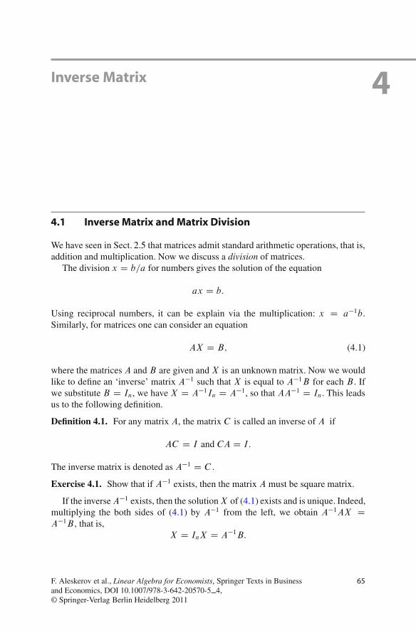
4Inverse Matrix
4.1 Inverse Matrix and Matrix Division
We have seen in Sect. 2.5 that matrices admit standard arithmetic operations, that is,addition and multiplication. Now we discuss a division of matrices.
The division x D b=a for numbers gives the solution of the equation
ax D b:
Using reciprocal numbers, it can be explain via the multiplication: x D a�1b.Similarly, for matrices one can consider an equation
AX D B; (4.1)
where the matrices A and B are given and X is an unknown matrix. Now we wouldlike to define an ‘inverse’ matrix A�1 such that X is equal to A�1B for each B . Ifwe substitute B D In, we have X D A�1In D A�1, so that AA�1 D In. This leadsus to the following definition.
Definition 4.1. For any matrix A, the matrix C is called an inverse of A if
AC D I and CA D I:
The inverse matrix is denoted as A�1 D C .
Exercise 4.1. Show that if A�1 exists, then the matrix A must be square matrix.
If the inverse A�1 exists, then the solution X of (4.1) exists and is unique. Indeed,multiplying the both sides of (4.1) by A�1 from the left, we obtain A�1AX DA�1B , that is,
X D InX D A�1B:
F. Aleskerov et al., Linear Algebra for Economists, Springer Texts in Businessand Economics, DOI 10.1007/978-3-642-20570-5 4,© Springer-Verlag Berlin Heidelberg 2011
65
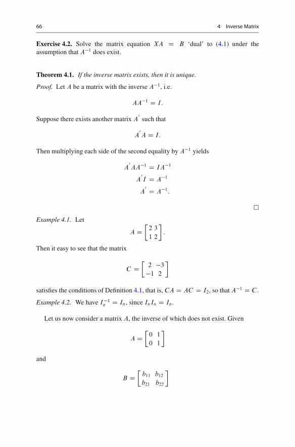
66 4 Inverse Matrix
Exercise 4.2. Solve the matrix equation XA D B ‘dual’ to (4.1) under theassumption that A�1 does exist.
Theorem 4.1. If the inverse matrix exists, then it is unique.
Proof. Let A be a matrix with the inverse A�1, i.e.
AA�1 D I:
Suppose there exists another matrix A0
such that
A0
A D I:
Then multiplying each side of the second equality by A�1 yields
A0
AA�1 D IA�1
A0
I D A�1
A0 D A�1:
�
Example 4.1. Let
A D�
2 3
1 2
�:
Then it easy to see that the matrix
C D�
2 �3
�1 2
�
satisfies the conditions of Definition 4.1, that is, CA D AC D I2, so that A�1 D C .
Example 4.2. We have I �1n D In, since InIn D In.
Let us now consider a matrix A, the inverse of which does not exist. Given
A D�
0 1
0 1
�
and
B D�
b11 b12
b21 b22
�
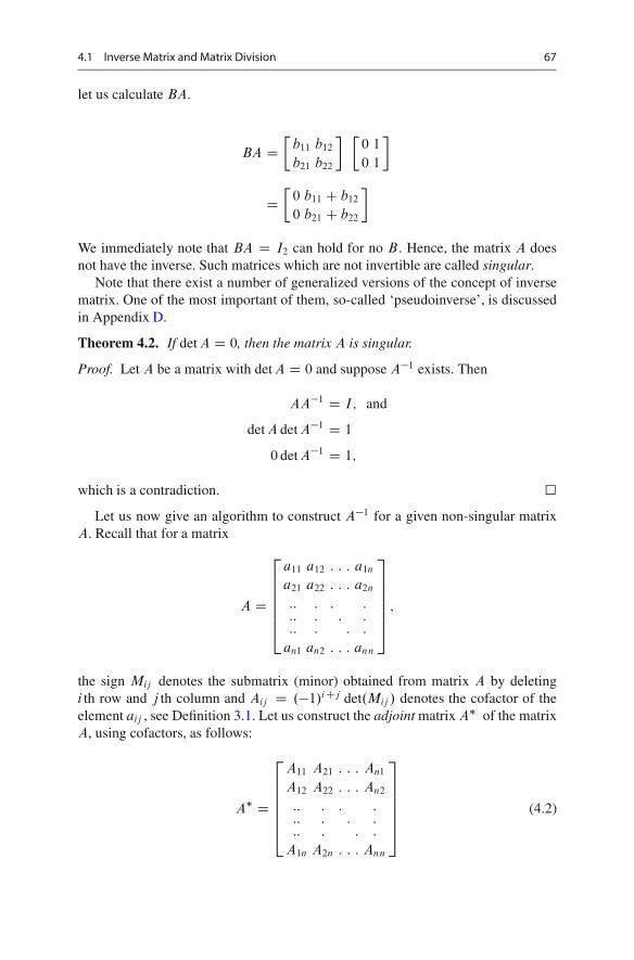
4.1 Inverse Matrix and Matrix Division 67
let us calculate BA.
BA D�
b11 b12
b21 b22
� �0 1
0 1
�
D�
0 b11 C b12
0 b21 C b22
�
We immediately note that BA D I2 can hold for no B . Hence, the matrix A doesnot have the inverse. Such matrices which are not invertible are called singular.
Note that there exist a number of generalized versions of the concept of inversematrix. One of the most important of them, so-called ‘pseudoinverse’, is discussedin Appendix D.
Theorem 4.2. If det A D 0, then the matrix A is singular.
Proof. Let A be a matrix with det A D 0 and suppose A�1 exists. Then
AA�1 D I; and
det A det A�1 D 1
0 det A�1 D 1;
which is a contradiction. �
Let us now give an algorithm to construct A�1 for a given non-singular matrixA. Recall that for a matrix
A D
2
666664
a11 a12 : : : a1n
a21 a22 : : : a2n
:: : : ::: : : ::: : : :
an1 an2 : : : ann
3
777775
;
the sign Mij denotes the submatrix (minor) obtained from matrix A by deletingi th row and j th column and Aij D .�1/iCj det.Mij / denotes the cofactor of theelement aij , see Definition 3.1. Let us construct the adjoint matrix A� of the matrixA, using cofactors, as follows:
A� D
2
666664
A11 A21 : : : An1
A12 A22 : : : An2
:: : : ::: : : ::: : : :
A1n A2n : : : Ann
3
777775
(4.2)
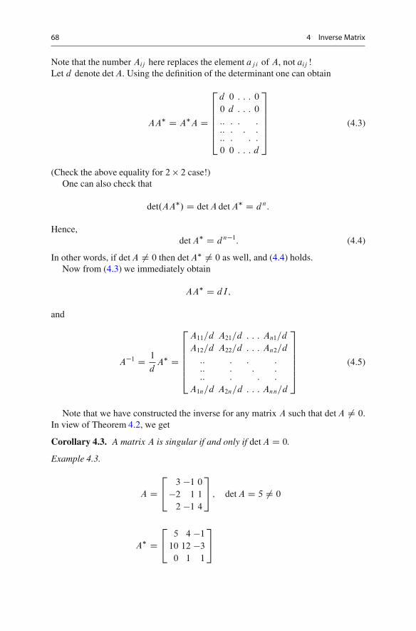
68 4 Inverse Matrix
Note that the number Aij here replaces the element aj i of A, not aij !Let d denote det A. Using the definition of the determinant one can obtain
AA� D A�A D
2
666664
d 0 : : : 0
0 d : : : 0
:: : : ::: : : ::: : : :
0 0 : : : d
3
777775
(4.3)
(Check the above equality for 2 � 2 case!)One can also check that
det.AA�/ D det A det A� D d n:
Hence,det A� D d n�1: (4.4)
In other words, if det A ¤ 0 then det A� ¤ 0 as well, and (4.4) holds.Now from (4.3) we immediately obtain
AA� D dI;
and
A�1 D 1
dA� D
2
666664
A11=d A21=d : : : An1=d
A12=d A22=d : : : An2=d
:: : : ::: : : ::: : : :
A1n=d A2n=d : : : Ann=d
3
777775
(4.5)
Note that we have constructed the inverse for any matrix A such that det A ¤ 0.In view of Theorem 4.2, we get
Corollary 4.3. A matrix A is singular if and only if det A D 0.
Example 4.3.
A D2
43 �1 0
�2 1 1
2 �1 4
3
5 ; det A D 5 ¤ 0
A� D2
45 4 �1
10 12 �3
0 1 1
3
5
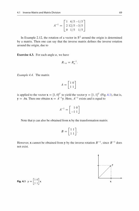
4.1 Inverse Matrix and Matrix Division 69
A�1 D2
41 4=5 �1=5
2 12=5 �3=5
0 1=5 1=5
3
5
In Example 2.12, the rotation of a vector in R2 around the origin is determinedby a matrix. Then one can say that the inverse matrix defines the inverse rotationaround the origin, due to
Exercise 4.3. For each angle ˛, we have
R�˛ D R�1˛ :
Example 4.4. The matrix
A D�
1 0
1 1
�
is applied to the vector x D Œ1; 0�T to yield the vector y D Œ1; 1�T (Fig. 4.1), that is,y D Ax. Then one obtains x D A�1y. Here, A�1 exists and is equal to
A�1 D�
1 0
�1 1
�
Note that y can also be obtained from x by the transformation matrix
B D�
1 1
1 1
�:
However, x cannot be obtained from y by the inverse rotation B�1, since B�1 doesnot exist.
Fig. 4.1 y D�1 0
1 1
�x
�
�
��
���
y
x
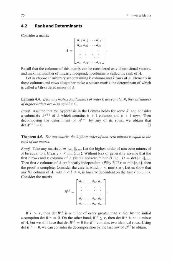
70 4 Inverse Matrix
4.2 Rank and Determinants
Consider a matrix
A D
2
666664
a11 a12 : : : a1n
a21 a22 : : : a2n
:: : : ::: : : ::: : : :
as1 as2 : : : asn
3
777775
:
Recall that the columns of this matrix can be considered as s-dimensional vectors,and maximal number of linearly independent columns is called the rank of A.
Let us choose an arbitrary set containing k columns and k rows of A. Elements inthese columns and rows altogether make a square matrix the determinant of whichis called a kth-ordered minor of A.
Lemma 4.4. If for any matrix A all minors of order k are equal to 0, then all minorsof higher orders are also equal to 0.
Proof. Assume that the hypothesis in the Lemma holds for some k, and considera submatrix AkC1 of A which contains k C 1 columns and k C 1 rows. Thendecomposing the determinant of AkC1 by any of its rows, we obtain thatdet AkC1 D 0. �
Theorem 4.5. For any matrix, the highest order of non-zero minors is equal to therank of the matrix.
Proof. Take any matrix A D kaij ks�n. Let the highest order of non-zero minors ofA be equal to r. Clearly r � minfs; ng. Without loss of generality assume that thefirst r rows and r columns of A yield a nonzero minor D, i.e., D D det kaij kr�r .Then first r columns of A are linearly independent. (Why ?) If r D minfs; ng, thenthe proof is complete. Consider the case in which r < minfs; ng. Let us show thatany l th column of A, with r < l � n, is linearly dependent on the first r columns.Consider the matrix
Bi;l D
2
666664
a11 : : : a1r a1l
: : : :: : : :: : : :
ar1 : : : arr arl
ai1 : : : air ail
3
777775
:
If i > r , then det Bi;l is a minor of order greater than r . So, by the initialassumption det Bi;l D 0. On the other hand, if i � r , then det Bi;l is not a minorof A, but we still have that det Bi;l D 0 for Bi;l contains two identical rows. Usingdet Bi;l D 0, we can consider its decomposition by the last row of Bi;l to obtain,

4.3 Problems 71
ai1A1 C ai2A2 C � � � C airAr C ailD D 0;
where Ak is the minor associated with the element aik of the matrix Bi;l . Note thatthe minor Ak is formed by the elements of the first r rows of A, so, the tuple ofcoefficients A1; : : : ; Ar here is the same for all i . Since D ¤ 0, we get
ail D �A1
Dai1 � � � � � Ar
Dair :
This equality holds for all i D 1; : : : ; s. So, i th column of A is the sum of first r
columns multiplied by coefficients .�A1=D; : : : ;�Ar=D/, respectively. �
In particular, a square matrix of order n has the maximal rank n if and only if itsdeterminant is non-zero. Such matrix is called a matrix of full rank.
Corollary 4.6. The maximal number of linearly independent rows of a matrixequals the maximal number of its linearly independent columns, that is, to the rankof the matrix.
Exercise 4.4. Consider the transpose matrix AT of A to prove the above claimyourself.
4.3 Problems
1. For each of the following matrix, find the inverse.
(a)
�1 2
3 4
�; (b)
�cos ˛ � sin ˛
sin ˛ cos ˛
�; (c)
2
42 7 3
3 9 4
1 5 3
3
5;
(d)
2
41 2 2
2 1 �2
2 �2 1
3
5; (e)
2
664
0 �2 1 5
10 0 �1 0
0 1 �1 2
1 2 �2 3
3
775.
2. Find the inverse of
(a)
2
6664
1 1 : : : 1 1
0 1 : : : 1 1:::
:::: : :
::::::
0 0 : : : 0 1
3
7775
; (b)
2
6664
1 1 1 : : : 1 1
1 0 1 : : : 1 1:::
::::::
: : ::::
:::
1 1 1 : : : 1 0
3
7775
; (c)
2
6664
0 1 1 : : : 1
1 0 1 : : : 1:::
::::::
: : ::::
1 1 1 : : : 0
3
7775
.
3. Solve for the matrix X in the following equations
(a)
�1 2
3 4
�X D
�3 5
5 a
�; (b) X
�3 �2
5 �4
�D��1 5
�2 6
�;

72 4 Inverse Matrix
(c) X
2
45 3 1
1 �3 �2
�5 2 1
3
5 D2
4�8 3 0
�5 9 0
�2 15 0
3
5;
(d)
2
42 �3 1
4 �5 2
5 �7 3
3
5X
2
49 7 6
1 1 2
1 1 1
3
5 D2
42 0 �2
18 12 9
23 15 11
3
5.
4. Let A and B be non-singular matrices of the order n. Show that the followingstatements are equivalent.
(a) AB D BA,
(b) AB�1 D B�1A,
(c) A�1B D BA�1,
(d) A�1B�1 D B�1A�1.5. Let A be symmetric non-singular matrix. Show that A�1 is also symmetric.6. Let A be a lower triangular (or an upper triangular) matrix. Show that A�1 is
also lower (respectively, upper) triangular.7. Find the rank of the matrix below for all possible values of �
(a)
2
41 � �1 2
2 �1 � 5
1 10 6 1
3
5;
(b)
2
664
0 �1 1 �1
� 0 �1 0
0 0 2� 2
1 2 �2 3
3
775.
8. Prove that adding a row to a matrix A either does not change the rank of A orincreases it by 1.
9. Find conditions which are necessary and sufficient for any three points.x1; y1/; .x2; y2/ and .x3; y3/ to be on the same line.
10. What are the necessary and sufficient conditions for the three lines
8<
:
a1x C b1y C c1 D 0
a2x C b2y C c2 D 0
a3x C b3y C c3 D 0
to intersect at one point?11. Let A D ��aij
��m�n
be a matrix, and write it as a set of columns
A D .A1; A2; : : : ; An/ :
4.3 Problems 73
Consider a matrix A0 such that(a) A0 D .A1; A2; : : : ; Ai�1; cAi ; AiC1; : : : ; An/ where c ¤ 0,(b) A0 D �A1; : : : ; Ai�1; Aj ; AiC1; : : : ; Aj �1; Ai ; Aj C1; : : : ; An
�.
Show that in both cases, matrix A0 has the same rank as A.12.* Prove that the rank of the sum of two matrices is not greater than the sum of
their ranks.13.* Matrix A is called nilpotent of degree k if Ak D 0.
Prove that if a square matrix A D ��aij
��
2�2of order two is nilpotent of some
positive degree k then A2 D 0.

•

5Systems of Linear Equations
Remember the economic model given in Introduction. It is one of the main problemsin economics to find when (i.e, under what price) the demand and the supply of theeconomic system will be in equilibrium. We now begin to find these conditions forour model in the most general way.
A set of linear equations is called a system. It is of interest to find conditions underwhich (a) the solution of a system exists, (b) the solution of a system is unique.
Example 5.1.
�x1 C 5x2 D 1
x1 C 5x2 D 7There is no solution of this system. Why?
�x1 C 2x2 D 7
x1 C x2 D 4The solution is unique: x1 D 1; x2 D 3:
�3x1 � x2 D 1
6x1 � 2x2 D 2
This system has many solutions:x1 D k 2 R; x2 D 3k � 1:
We will discuss three approaches to solutions of such systems. First of them,so-called Cramer method, gives simple formulae for the solution, see Sect. 5.1.However, this method is used only for special systems. The second approach isbased on a universal algorithm for solution of the system, see Sect. 5.2. However,the dependence of the solution on the data is not clear in the algorithm. The thirdapproach gives an explicit formula for a particular or an approximate solution. It isbased on the concept of a pseudoinverse of a matrix, see Appendix D.
Consider now a system of linear equations
8ˆ<
ˆ:
a11x1 C a12x2 C : : : C a1nxn D b1
a21x1 C a22x2 C : : : C a2nxn D b2
: : : : : : : : : : : : : : : :
as1x1 C as2x2 C : : : C asnxn D bs
(5.1)
F. Aleskerov et al., Linear Algebra for Economists, Springer Texts in Businessand Economics, DOI 10.1007/978-3-642-20570-5 5,© Springer-Verlag Berlin Heidelberg 2011
75
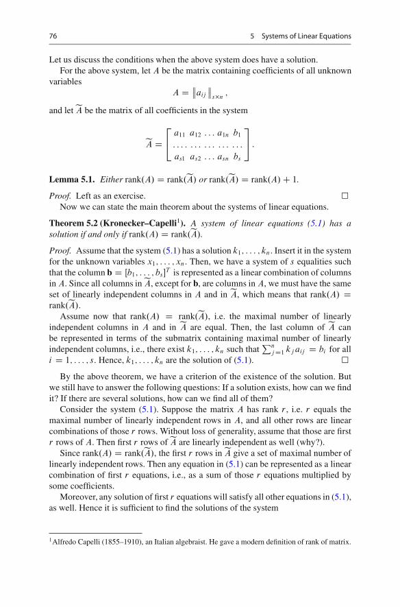
76 5 Systems of Linear Equations
Let us discuss the conditions when the above system does have a solution.For the above system, let A be the matrix containing coefficients of all unknown
variablesA D ��aij
��
s�n;
and let eA be the matrix of all coefficients in the system
eA D2
4a11 a12 : : : a1n b1
: : : : : : : : : : : : : : : :
as1 as2 : : : asn bs
3
5 :
Lemma 5.1. Either rank.A/ D rank.eA/ or rank.eA/ D rank.A/C 1.
Proof. Left as an exercise. �Now we can state the main theorem about the systems of linear equations.
Theorem 5.2 (Kronecker–Capelli1). A system of linear equations (5.1) has asolution if and only if rank.A/ D rank.eA/.
Proof. Assume that the system (5.1) has a solution k1; : : : ; kn. Insert it in the systemfor the unknown variables x1; : : : ; xn. Then, we have a system of s equalities suchthat the column b D Œb1; : : : ; bs�
T is represented as a linear combination of columnsin A. Since all columns in eA, except for b, are columns in A, we must have the sameset of linearly independent columns in A and in eA, which means that rank.A/ Drank.eA/.
Assume now that rank.A/ D rank.eA/, i.e. the maximal number of linearlyindependent columns in A and in eA are equal. Then, the last column of eA canbe represented in terms of the submatrix containing maximal number of linearlyindependent columns, i.e., there exist k1; : : : ; kn such that
Pnj D1 kj aij D bi for all
i D 1; : : : ; s. Hence, k1; : : : ; kn are the solution of (5.1). �
By the above theorem, we have a criterion of the existence of the solution. Butwe still have to answer the following questions: If a solution exists, how can we findit? If there are several solutions, how can we find all of them?
Consider the system (5.1). Suppose the matrix A has rank r , i.e. r equals themaximal number of linearly independent rows in A, and all other rows are linearcombinations of those r rows. Without loss of generality, assume that those are firstr rows of A. Then first r rows of eA are linearly independent as well (why?).
Since rank.A/ D rank.eA/, the first r rows in eA give a set of maximal number oflinearly independent rows. Then any equation in (5.1) can be represented as a linearcombination of first r equations, i.e., as a sum of those r equations multiplied bysome coefficients.
Moreover, any solution of first r equations will satisfy all other equations in (5.1),as well. Hence it is sufficient to find the solutions of the system
1Alfredo Capelli (1855–1910), an Italian algebraist. He gave a modern definition of rank of matrix.

5 Systems of Linear Equations 77
8ˆ<
ˆ:
a11x1 C a12x2 C : : : C a1nxn D b1
a21x1 C a22x2 C : : : C a2nxn D b2
: : : : : : : : : : : : : : : :
ar1x1 C ar2x2 C : : : C arnxn D br
(5.2)
We can rewrite the above system as A0x0 D b0, where A0 D kaij kr�n, x0 DŒx1; : : : ; xn�T and b0 D Œb1; : : : ; br �T . The matrix A
0
has a rank r . (Why?)If r D n then the number of equations is equal to the number of variables, and
the system (5.2) has a unique solution
x0 D�A
0
��1
b0:
If r < n , then detkaij kr�r is not equal to 0. Then reconstruct (5.2) as
8<
:
a11x1 C : : : C a1r xr D b1 � a1;rC1xrC1 � � � � � a1nxn
: : : : : : : : : : : : :
ar1x1 C : : : C arr xr D br � ar;rC1xrC1 � � � � � arnxn
(5.3)
or A00
x00 D b
00
where A00 D kaij kr�r , x
00 D Œx1; : : : ; xr �T and b00 D Œˇ1; : : : ; ˇn�T
with ˇi D bi � ai;rC1xrC1 � � � � � ainxn.Choose some arbitrary (!) values crC1; : : : ; cn for variables xrC1; : : : ; xn. Then
we obtain the system of r equations in r unknown variables with det A00 ¤ 0.
Hence the system (5.3) has a solution
x00 D
�A
00
��1
b00
: (5.4)
Let x00 D Œc1; : : : ; cr �
T . It is obvious that Œc1; : : : ; cr ; crC1; : : : ; cn�T is then asolution of (5.2).
We can now formulate the general rule of obtaining the solutions of a system.Let a system (5.1) be given such that rank.A/ D rank.eA/ D r . Choose r linearly
independent rows in A and retain in (4.3) only the equations associated with r
linearly independent rows that you chose. Keep at the left side of these equationsonly r variables such that the determinant of the associated coefficients for thesevariables is not equal to 0. For each equation, put all other variables, that are calledfree, in the right side of the equations. Assign to the free variables arbitrary values,and calculating values of all other variables by (5.4), we obtain all solutions of (4.3).
Example 5.2. Consider the following system of equations:
8<
:
x1 C x2 � 2x3 � x4 C x5 D 1
3x1 � x2 C x3 C 4x4 C 3x5 D 4
x1 C 5x2 � 9x3 � 8x4 C x5 D 0

78 5 Systems of Linear Equations
Check that rank.A/ D rank.eA/ D 2. First and third equations are linearlyindependent. So, we have to consider only:
(x1 C x2 D 1C 2x3 C x4 � x5
x1 C 5x2 D 9x3 C 8x4 � x5
Then
x1 D 5
4C 1
4x3 � 3
4x4 � x5
x2 D �1
4C 7
4x3 C 7
4x4
where x1; x2; x3 2 R. This is the general solution.
Corollary 5.3. The solution of system (4.3), whenever exists, is unique if and onlyif rank.A/ is equal to the number of variables.
5.1 The Case of Unique Solution: Cramer’s Rule
We have seen in (3.5) that the components of a solution for a system of twolinear equations with two variables is expressed as ratios of determinants of certainmatrices. Let us give analogous formulae for larger systems.
Theorem 5.4 (Cramer’s2 rule). Let
AX D B
be a system of linear equations such that the number of equations and the numberof variables are the same, that is, A is a square matrix of order n. Suppose that A isnot singular. Then the solution of the system is
xi D det Ai
det A
for all i D 1; : : : ; n, where Ai is the matrix formed from A by replacing its i -thcolumn by the column B .
Proof. From the equationAX D B
2Gabriel Cramer (1704–1752) was a Swiss mathematician who introduced determinants and usedthem to solve algebraic equations.
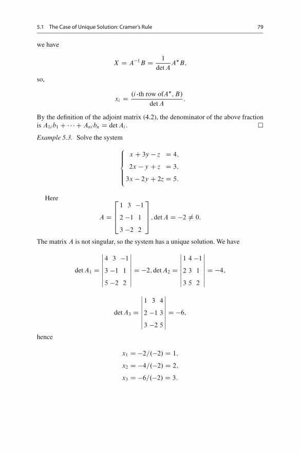
5.1 The Case of Unique Solution: Cramer’s Rule 79
we have
X D A�1B D 1
det AA�B;
so,
xi D .i -th row ofA�; B/
det A:
By the definition of the adjoint matrix (4.2), the denominator of the above fractionis A1i b1 C � � � C Anibn D det Ai . �
Example 5.3. Solve the system
8ˆ<
ˆ:
x C 3y � z D 4;
2x � y C z D 3;
3x � 2y C 2z D 5:
Here
A D
2
664
1 3 �1
2 �1 1
3 �2 2
3
775 ; det A D �2 ¤ 0:
The matrix A is not singular, so the system has a unique solution. We have
det A1 D
ˇˇˇˇˇˇˇ
4 3 �1
3 �1 1
5 �2 2
ˇˇˇˇˇˇˇ
D �2; det A2 D
ˇˇˇˇˇˇˇ
1 4 �1
2 3 1
3 5 2
ˇˇˇˇˇˇˇ
D �4;
det A3 D
ˇˇˇˇˇˇˇ
1 3 4
2 �1 3
3 �2 5
ˇˇˇˇˇˇˇ
D �6;
hence
x1 D �2=.�2/ D 1;
x2 D �4=.�2/ D 2;
x3 D �6=.�2/ D 3:
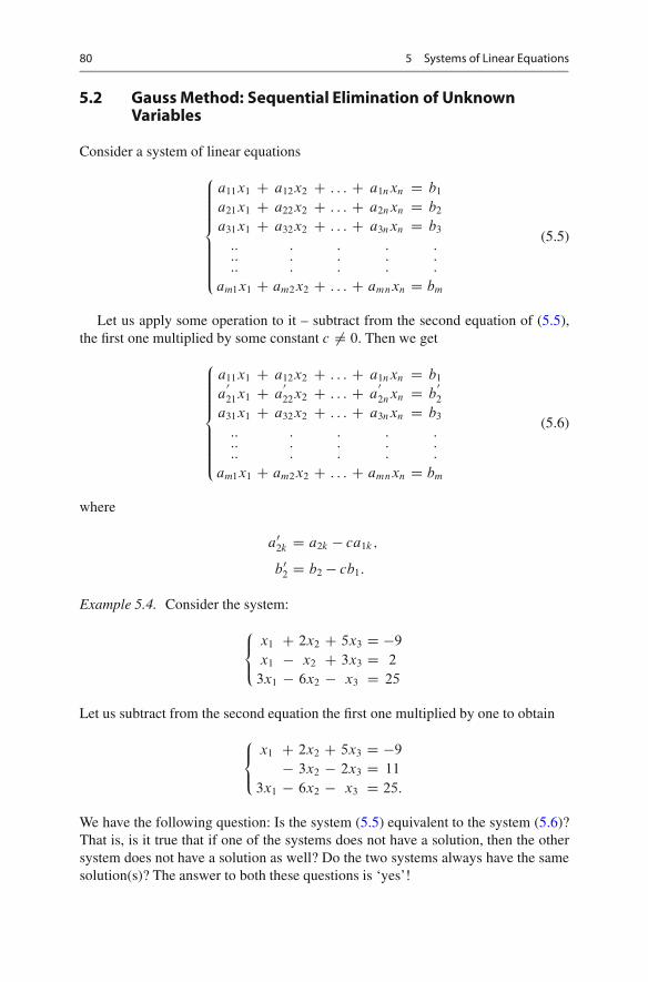
80 5 Systems of Linear Equations
5.2 Gauss Method: Sequential Elimination of UnknownVariables
Consider a system of linear equations
8ˆˆˆ<
ˆˆˆ:
a11x1 C a12x2 C : : : C a1nxn D b1
a21x1 C a22x2 C : : : C a2nxn D b2
a31x1 C a32x2 C : : : C a3nxn D b3
:: : : : ::: : : : ::: : : : :
am1x1 C am2x2 C : : : C amnxn D bm
(5.5)
Let us apply some operation to it – subtract from the second equation of (5.5),the first one multiplied by some constant c ¤ 0. Then we get
8ˆˆˆ<
ˆˆˆ:
a11x1 C a12x2 C : : : C a1nxn D b1
a0
21x1 C a0
22x2 C : : : C a0
2nxn D b0
2
a31x1 C a32x2 C : : : C a3nxn D b3
:: : : : ::: : : : ::: : : : :
am1x1 C am2x2 C : : : C amnxn D bm
(5.6)
where
a02k D a2k � ca1k;
b02 D b2 � cb1:
Example 5.4. Consider the system:
8<
:
x1 C 2x2 C 5x3 D �9
x1 � x2 C 3x3 D 2
3x1 � 6x2 � x3 D 25
Let us subtract from the second equation the first one multiplied by one to obtain
8<
:
x1 C 2x2 C 5x3 D �9
� 3x2 � 2x3 D 11
3x1 � 6x2 � x3 D 25:
We have the following question: Is the system (5.5) equivalent to the system (5.6)?That is, is it true that if one of the systems does not have a solution, then the othersystem does not have a solution as well? Do the two systems always have the samesolution(s)? The answer to both these questions is ‘yes’!

5.2 Gauss Method: Sequential Elimination of Unknown Variables 81
Lemma 5.5. Systems (5.5) and (5.6) are equivalent.
Note that the matrix eA for the system (5.6) is obtained from the matrix eA of thesystem (5.5) via an elementary transformation of the third type (see Sect. 2.8). So,it follows from Lemma 5.5 that any elementary transformation, being applied to thematrix eA of a system of linear equations, gives the matrix of an equivalent system.
Proof. Let .k1; : : : ; kn/ be a solution of (5.5). Let us show that it is also a solutionof (5.6). Then it remains to prove that .k1; : : : ; kn/ satisfies the second equation in(5.6), for it clearly satisfies all other equations. Note that we have
a11k1 C a12k2 C � � � C a1nkn D b1
a21k1 C a22k2 C � � � C a2nkn D b2:
Multiplying the first equality by c and subtracting it from the second one gives
.a21 � ca11/k1 C .a22 � ca12/k2 C � � � C .a2n � ca1n/kn D b2 � cb1
ora0
21k1 C a022k2 C � � � C a0
2nkn D b02:
So .k1; : : : ; kn/ is also a solution of (5.6). It is left as an exercise to show that anysolution of (5.6) is a solution of (5.5) as well. �
It is obvious that such transformations of a system, if applied several times, stillyield an equivalent system.
Remark 5.1. By this method, we can exclude step by step some variables from eachequation in the system. If, at the end, we obtain an equation, say the i th one, suchthat all coefficients of unknown variables in it are equal to 0 as well as the right handside of it (call it Qbi ), then we can just omit this equation. But, if Qbi is not zero whileall unknown variables have zero coefficients in the i th equation, then that equationcan not be satisfied by any values of variables. In that case, the system (5.5) is calledinconsistent.
Now we are ready to give the Gauss method.Let the system (5.5) be given. Relabel all coefficients aij by a0
ij and bi by b0i , for
all i and j . Let i and j be two counters (i for rows and j for variables) with theinitial values being equal to 1, i.e., i WD 1 and j WD 1.
Procedure begins atStep 1: Determine if ai�1
ij ¤ 0. If ai�1ij D 0, then look for a row k 2 fi C 1; : : : ; mg
such that akj ¤ 0. If there is no such k, go to Step 4. Otherwise, choosesuch a k; interchange rows i and k, and switch the labels of the coefficients,i.e., ai�1
il $ ai�1kl and bi�1
i $ bi�1k , for all l D 1; : : : ; n.
Step 2: To exclude xj from all equations indexed by k D i C 1; : : : ; m, subtractfrom the kth equation the i th one multiplied by ai�1
kj =ai�1ij , and obtain the
reduced coefficients
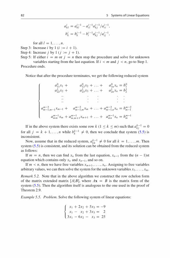
82 5 Systems of Linear Equations
aikl D ai�1
kl � ai�1il ai�1
kj =ai�1i i ;
bik D bi�1
k � bi�1i ai�1
kj =ai�1ij ;
for all l D 1; : : : ; n.Step 3: Increase i by 1 (i WD i C 1).Step 4: Increase j by 1 (j WD j C 1).Step 5: If either i D m or j D n then stop the procedure and solve for unknown
variables starting from the last equation. If i < m and j < n, go to Step 1.Procedure ends.
Notice that after the procedure terminates, we get the following reduced system
8ˆˆˆˆ<
ˆˆˆˆ:
a011x1 C a0
12x2 C : : : C a01nxn D b0
1
a122x2 C a1
23x3 C : : : C a12nxn D b1
2
:: : : : ::: : : : ::: : : : :
am�2m�1;m�1xm�1 C am�2
m�1;mxm C : : : C am�2m�1;nxn D bm�2
m�1
am�1mm xm C am�1
m;mC1xmC1 C : : : C am�1mn xn D bm�1
m
If in the above system there exists some row k (1 � k � m) such that ak�1kj D 0
for all j D k C 1; : : : ; n while bk�1k ¤ 0, then we conclude that system (5.5) is
inconsistent.Now, assume that in the reduced system, ak�1
kk ¤ 0 for all k D 1; : : : ; m. Thensystem (5.5) is consistent, and its solution can be obtained from the reduced systemas follows:
If m D n, then we can find xn from the last equation, xn�1 from the .n � 1/stequation which contains only xn and xn�1, and so on.
If m < n, then we have free variables xmC1; : : : :; xn. Assigning to free variablesarbitrary values, we can then solve the system for the unknown variables x1; : : : ; xm.
Remark 5.2. Note that in the above algorithm we construct the row echelon formof the matrix extended matrix ŒAjB�, where Ax D B is the matrix form of thesystem (5.5). Then the algorithm itself is analogous to the one used in the proof ofTheorem 2.9.
Example 5.5. Problem. Solve the following system of linear equations:
8<
:
x1 C 2x2 C 5x3 D �9
x1 � x2 C 3x3 D 2
3x1 � 6x2 � x3 D 25

5.2 Gauss Method: Sequential Elimination of Unknown Variables 83
Solution. Let us construct extended matrix of this system and apply Gauss elimina-tion procedure to get
2
41 2 5 �9
1 �1 3 2
3 �6 �1 25
3
5!2
41 2 5 �9
0 �3 �2 11
0 �12 �16 52
3
5!
2
41 2 5 �9
0 �3 �2 11
0 0 �8 8
3
5 :
Thus, we have:x1 C 2x2 C 5x3 D �9
� 3x2 � 2x3 D 11
� 8x3 D 8
From the last equation, we have x3 D �1. Substitute the value x3 D �1 in thesecond equation and get �3x2 C 2 D 11, hence x2 D �3. Then substitute thesevalues of x2 and x3 to the first equation and get x1 � 6 � 5 D �9, or x1 D 2.
To avoid non-necessary fractions, one can multiply each row by a nonzeronumber (say, by the denominator aij of the fractions in Step 2) in each stage ofalgorithm.
Example 5.6. Problem. Solve the system of linear equations
8ˆ<
ˆ:
x1 � 5x2 � 8x3 C x4 D 3
3x1 C x2 � 3x3 � 5x4 D 1
x1 � 7x3 C 2x4 D �5
� 11x2 C 20x3 � 9x4 D 2
Solution. Applying Gauss elimination procedure on the extended coefficient matrixwe obtain
2
664
1 �5 �8 1 3
3 1 �3 �5 1
1 0 �7 2 �5
0 11 20 �9 2
3
775!
2
664
1 �5 �8 1 3
0 16 21 �8 �8
0 5 1 1 �8
0 11 20 �9 2
3
775!
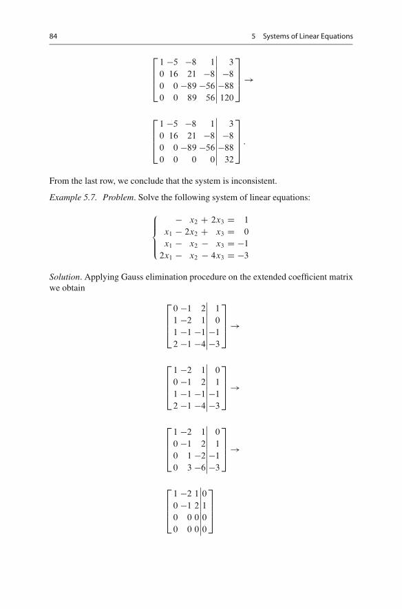
84 5 Systems of Linear Equations
2
664
1 �5 �8 1 3
0 16 21 �8 �8
0 0 �89 �56 �88
0 0 89 56 120
3
775!
2
664
1 �5 �8 1 3
0 16 21 �8 �8
0 0 �89 �56 �88
0 0 0 0 32
3
775 :
From the last row, we conclude that the system is inconsistent.
Example 5.7. Problem. Solve the following system of linear equations:
8ˆ<
ˆ:
� x2 C 2x3 D 1
x1 � 2x2 C x3 D 0
x1 � x2 � x3 D �1
2x1 � x2 � 4x3 D �3
Solution. Applying Gauss elimination procedure on the extended coefficient matrixwe obtain
2
664
0 �1 2 1
1 �2 1 0
1 �1 �1 �1
2 �1 �4 �3
3
775!
2
664
1 �2 1 0
0 �1 2 1
1 �1 �1 �1
2 �1 �4 �3
3
775!
2
664
1 �2 1 0
0 �1 2 1
0 1 �2 �1
0 3 �6 �3
3
775!
2
664
1 �2 1 0
0 �1 2 1
0 0 0 0
0 0 0 0
3
775

5.3 Homogeneous Equations 85
Thus, we have �x1 � 2x2 C x3 D 0
� x2 C 2x3 D 1
Take one of the variables in the last equation, say, x3, as a free variable. Then wehave x2 D 2x3 � 1, where x3 is an arbitrary real number. From the first equation,we get x1 D 2x2 � x3 D 3x3 � 2.
5.3 Homogeneous Equations
Consider the system:
8ˆˆ<
ˆˆ:
a11x1 C a12x2 C : : : C a1nxn D 0
a21x1 C a22x2 C : : : C a2nxn D 0
:: : : : ::: : : : ::: : : : :
as1x1 C as2x2 C : : : C asnxn D 0
(5.7)
By Kronecker-Capelli Theorem, it follows that the above system has a solution.Indeed, it has a trivial solution given by .x1; x2; : : : ; xn/ D .0; 0; : : : ; 0/.
Any system which admits the zero vector as a solution is called a homogeneoussystem. Obviously, if the right hand-side of any equation in (5.7) were not zero, thenthe system could not admit the trivial solution, and will be called nonhomogeneous.
In the case of homogeneous system, the Kronecker-Capelli Theorem has asimpler form.
Theorem 5.6. LetAx D 0
be a homogeneous system of linear equations of n variables. Then either rank A D n
and the system has the unique zero solution or rank A < n and the system hasinfinitely many solutions.
Proof. Left as an exercise. (Hint. Use Gauss elimination procedure. How the rowechelon form of the matrix eA depends on rank A?) �
Consider an economy with m agents exchanging n kinds of goods. Let aij be thequantity of good i received (sold) by an agent j . If aij is positive, then we considerthat the good i is sold by agent j ; if aij is negative, then the amount jaij j is boughtby agent j .
Then.a1j ; a2j ; : : : ; anj /
is the vector showing the ‘exchanges’ of agent j of any good i D 1; : : : ; n.Similarly, the components of the vector
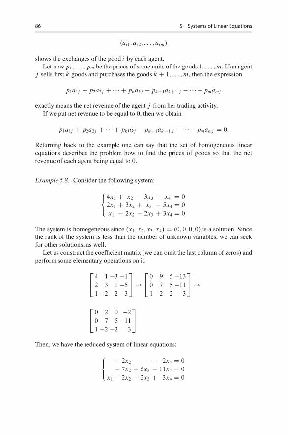
86 5 Systems of Linear Equations
.ai1; ai2; : : : ; aim/
shows the exchanges of the good i by each agent.Let now p1; : : : ; pm be the prices of some units of the goods 1; : : : ; m. If an agent
j sells first k goods and purchases the goods k C 1; : : : ; m, then the expression
p1a1j C p2a2j C � � � C pkakj � pkC1akC1;j � � � � � pmamj
exactly means the net revenue of the agent j from her trading activity.If we put net revenue to be equal to 0, then we obtain
p1a1j C p2a2j C � � � C pkakj � pkC1akC1;j � � � � � pmamj D 0:
Returning back to the example one can say that the set of homogeneous linearequations describes the problem how to find the prices of goods so that the netrevenue of each agent being equal to 0.
Example 5.8. Consider the following system:
8<
:
4x1 C x2 � 3x3 � x4 D 0
2x1 C 3x2 C x3 � 5x4 D 0
x1 � 2x2 � 2x3 C 3x4 D 0
The system is homogeneous since .x1; x2; x3; x4/ D .0; 0; 0; 0/ is a solution. Sincethe rank of the system is less than the number of unknown variables, we can seekfor other solutions, as well.
Let us construct the coefficient matrix (we can omit the last column of zeros) andperform some elementary operations on it.
2
44 1 �3 �1
2 3 1 �5
1 �2 �2 3
3
5!2
40 9 5 �13
0 7 5 �11
1 �2 �2 3
3
5!
2
40 2 0 �2
0 7 5 �11
1 �2 �2 3
3
5
Then, we have the reduced system of linear equations:
8<
:
� 2x2 � 2x4 D 0
� 7x2 C 5x3 � 11x4 D 0
x1 � 2x2 � 2x3 C 3x4 D 0
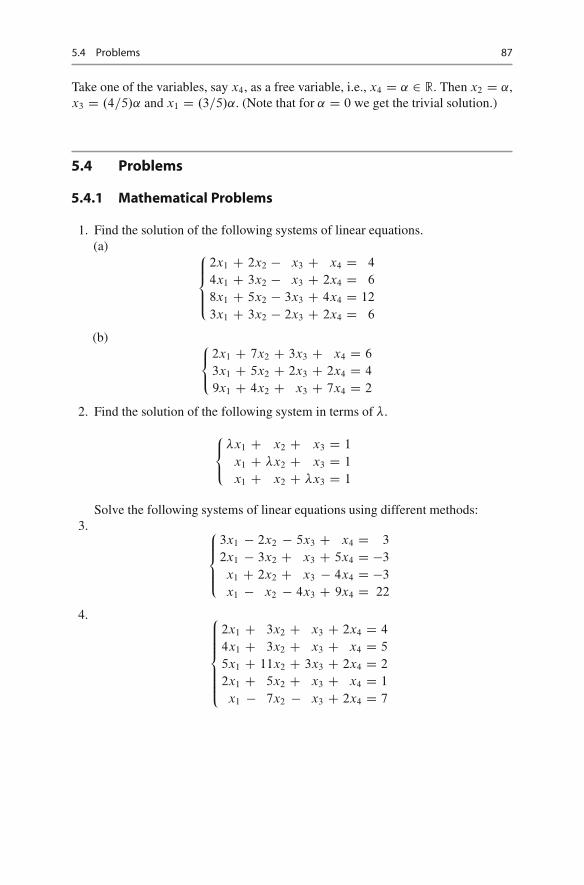
5.4 Problems 87
Take one of the variables, say x4, as a free variable, i.e., x4 D ˛ 2 R. Then x2 D ˛,x3 D .4=5/˛ and x1 D .3=5/˛. (Note that for ˛ D 0 we get the trivial solution.)
5.4 Problems
5.4.1 Mathematical Problems
1. Find the solution of the following systems of linear equations.(a) 8
ˆ<
ˆ:
2x1 C 2x2 � x3 C x4 D 4
4x1 C 3x2 � x3 C 2x4 D 6
8x1 C 5x2 � 3x3 C 4x4 D 12
3x1 C 3x2 � 2x3 C 2x4 D 6
(b) 8<
:
2x1 C 7x2 C 3x3 C x4 D 6
3x1 C 5x2 C 2x3 C 2x4 D 4
9x1 C 4x2 C x3 C 7x4 D 2
2. Find the solution of the following system in terms of �.
8<
:
�x1 C x2 C x3 D 1
x1 C �x2 C x3 D 1
x1 C x2 C �x3 D 1
Solve the following systems of linear equations using different methods:3. 8
ˆ<
ˆ:
3x1 � 2x2 � 5x3 C x4 D 3
2x1 � 3x2 C x3 C 5x4 D �3
x1 C 2x2 C x3 � 4x4 D �3
x1 � x2 � 4x3 C 9x4 D 22
4. 8ˆˆ<
ˆˆ:
2x1 C 3x2 C x3 C 2x4 D 4
4x1 C 3x2 C x3 C x4 D 5
5x1 C 11x2 C 3x3 C 2x4 D 2
2x1 C 5x2 C x3 C x4 D 1
x1 � 7x2 � x3 C 2x4 D 7
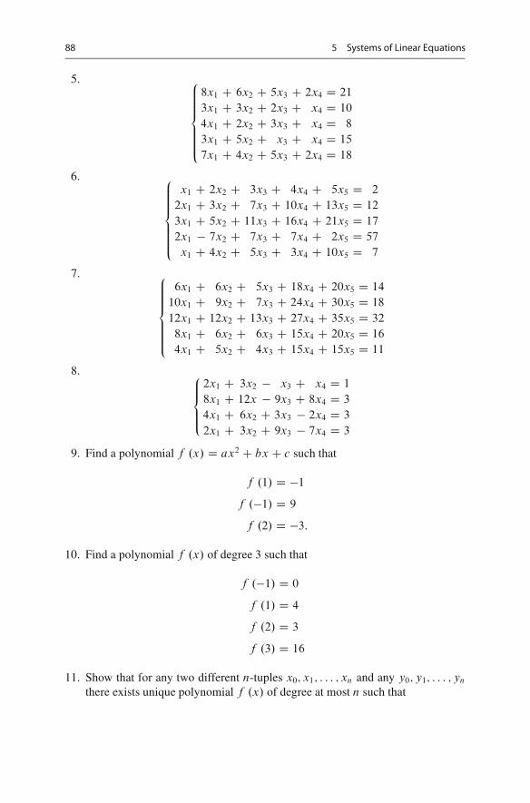
88 5 Systems of Linear Equations
5. 8ˆˆ<
ˆˆ:
8x1 C 6x2 C 5x3 C 2x4 D 21
3x1 C 3x2 C 2x3 C x4 D 10
4x1 C 2x2 C 3x3 C x4 D 8
3x1 C 5x2 C x3 C x4 D 15
7x1 C 4x2 C 5x3 C 2x4 D 18
6. 8ˆˆ<
ˆˆ:
x1 C 2x2 C 3x3 C 4x4 C 5x5 D 2
2x1 C 3x2 C 7x3 C 10x4 C 13x5 D 12
3x1 C 5x2 C 11x3 C 16x4 C 21x5 D 17
2x1 � 7x2 C 7x3 C 7x4 C 2x5 D 57
x1 C 4x2 C 5x3 C 3x4 C 10x5 D 7
7. 8ˆˆ<
ˆˆ:
6x1 C 6x2 C 5x3 C 18x4 C 20x5 D 14
10x1 C 9x2 C 7x3 C 24x4 C 30x5 D 18
12x1 C 12x2 C 13x3 C 27x4 C 35x5 D 32
8x1 C 6x2 C 6x3 C 15x4 C 20x5 D 16
4x1 C 5x2 C 4x3 C 15x4 C 15x5 D 11
8. 8ˆ<
ˆ:
2x1 C 3x2 � x3 C x4 D 1
8x1 C 12x � 9x3 C 8x4 D 3
4x1 C 6x2 C 3x3 � 2x4 D 3
2x1 C 3x2 C 9x3 � 7x4 D 3
9. Find a polynomial f .x/ D ax2 C bx C c such that
f .1/ D �1
f .�1/ D 9
f .2/ D �3:
10. Find a polynomial f .x/ of degree 3 such that
f .�1/ D 0
f .1/ D 4
f .2/ D 3
f .3/ D 16
11. Show that for any two different n-tuples x0; x1; : : : ; xn and any y0; y1; : : : ; yn
there exists unique polynomial f .x/ of degree at most n such that
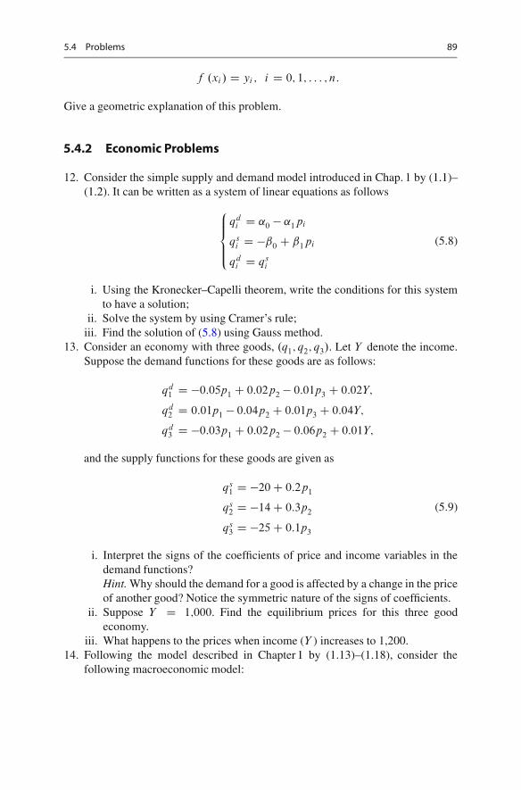
5.4 Problems 89
f .xi / D yi ; i D 0; 1; : : : ; n:
Give a geometric explanation of this problem.
5.4.2 Economic Problems
12. Consider the simple supply and demand model introduced in Chap. 1 by (1.1)–(1.2). It can be written as a system of linear equations as follows
8ˆ<
ˆ:
qdi D ˛0 � ˛1pi
qsi D �ˇ0 C ˇ1pi
qdi D qs
i
(5.8)
i. Using the Kronecker–Capelli theorem, write the conditions for this systemto have a solution;
ii. Solve the system by using Cramer’s rule;iii. Find the solution of (5.8) using Gauss method.
13. Consider an economy with three goods, .q1; q2; q3/. Let Y denote the income.Suppose the demand functions for these goods are as follows:
qd1 D �0:05p1 C 0:02p2 � 0:01p3 C 0:02Y;
qd2 D 0:01p1 � 0:04p2 C 0:01p3 C 0:04Y;
qd3 D �0:03p1 C 0:02p2 � 0:06p2 C 0:01Y;
and the supply functions for these goods are given as
qs1 D �20C 0:2p1
qs2 D �14C 0:3p2
qs3 D �25C 0:1p3
(5.9)
i. Interpret the signs of the coefficients of price and income variables in thedemand functions?Hint. Why should the demand for a good is affected by a change in the priceof another good? Notice the symmetric nature of the signs of coefficients.
ii. Suppose Y D 1;000. Find the equilibrium prices for this three goodeconomy.
iii. What happens to the prices when income (Y ) increases to 1,200.14. Following the model described in Chapter 1 by (1.13)–(1.18), consider the
following macroeconomic model:
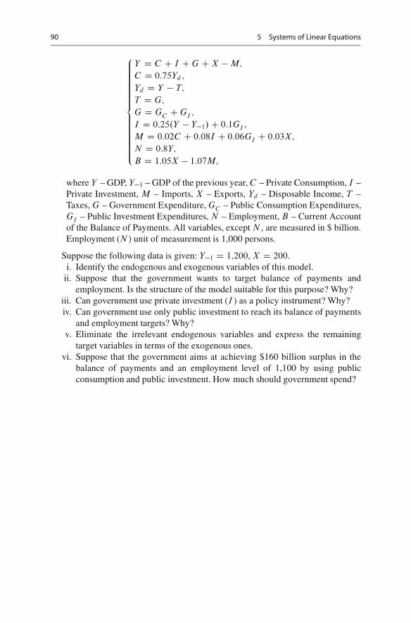
90 5 Systems of Linear Equations
8ˆˆˆˆˆˆ<
ˆˆˆˆˆˆ:
Y D C C I CG CX �M;
C D 0:75Yd ;
Yd D Y � T;
T D G;
G D GC CGI ;
I D 0:25.Y � Y�1/C 0:1GI ;
M D 0:02C C 0:08I C 0:06GI C 0:03X;
N D 0:8Y;
B D 1:05X � 1:07M;
where Y – GDP, Y�1 – GDP of the previous year, C – Private Consumption, I –Private Investment, M – Imports, X – Exports, Yd – Disposable Income, T –Taxes, G – Government Expenditure, GC – Public Consumption Expenditures,GI – Public Investment Expenditures, N – Employment, B – Current Accountof the Balance of Payments. All variables, except N , are measured in $ billion.Employment (N ) unit of measurement is 1,000 persons.
Suppose the following data is given: Y�1 D 1;200, X D 200.i. Identify the endogenous and exogenous variables of this model.
ii. Suppose that the government wants to target balance of payments andemployment. Is the structure of the model suitable for this purpose? Why?
iii. Can government use private investment (I ) as a policy instrument? Why?iv. Can government use only public investment to reach its balance of payments
and employment targets? Why?v. Eliminate the irrelevant endogenous variables and express the remaining
target variables in terms of the exogenous ones.vi. Suppose that the government aims at achieving $160 billion surplus in the
balance of payments and an employment level of 1,100 by using publicconsumption and public investment. How much should government spend?
6Linear Spaces
We now construct a generalization of the notions studied in the previous chapters.Consider some set L of elements x; y; z; : : : . We call L a linear space1 ifi. for any x; y 2 L, there exists some z 2 L such that
z D xC yI
ii. for any x 2 L and any real number �, we have �x 2 L.Elements of linear spaces are called vectors. (Here, the word ‘vector’ is used in
the abstract sense; it can represent a matrix, a function, a real vector, etc.) The linearspace is also called a vector space.
The vector operationsC (vector addition) and � (dot multiplication) must satisfythe following axioms on L
I-(i) xC y D yC x (commutativity),I-(ii) .xC y/C z D xC .yC z/ (associativity),
I-(iii) there exists a (null) element 0 such that xC 0 D 0C x D x for all x,I-(iv) for all x, there exists the additive inverse, .�x/, such that xC .�x/ D 0.II-(i) 1.x/ D x,
II-(ii) ˛.ˇx/ D .˛ˇ/x.III-(i) .˛ C ˇ/x D ˛xC ˇx,
III-(ii) ˛.xC y/ D ˛xC ˛y.Note that C and � are abstract operations, they are not necessarily addition and
multiplication defined on real numbers.
Example 6.1. Consider the set of all vectors in Rn. Show that under the standardoperations of vector addition and multiplication by a number (Sect. 2.1), this set isa linear space; check that all 8 axioms above are satisfied.
1In mathematics, a space is an abstract set of points with some additional structure. Mathematicalspaces are often considered as models for real physical spaces. In addition to linear spaces, thereare so-called Euclidean spaces, metric spaces, topological spaces and many others.
F. Aleskerov et al., Linear Algebra for Economists, Springer Texts in Businessand Economics, DOI 10.1007/978-3-642-20570-5 6,© Springer-Verlag Berlin Heidelberg 2011
91
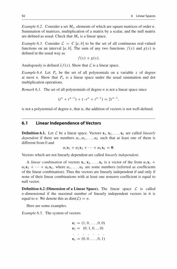
92 6 Linear Spaces
Example 6.2. Consider a set Mn, elements of which are square matrices of order n.Summation of matrices, multiplication of a matrix by a scalar, and the null matrixare defined as usual. Check that Mn is a linear space.
Example 6.3. Consider L D C Œa; b� to be the set of all continuous real-valuedfunctions on an interval Œa; b�. The sum of any two functions f .x/ and g.x/ isdefined in the usual way as
f .x/C g.x/:
Analogously is defined �f .x/. Show that L is a linear space.
Example 6.4. Let Pn be the set of all polynomials on a variable x of degreeat most n. Show that Pn is a linear space under the usual summation and dotmultiplication operations.
Remark 6.1. The set of all polynomials of degree n is not a linear space since
.tn C tn�1/C .�tn C tn�1/ D 2tn�1;
is not a polynomial of degree n, that is, the addition of vectors is not well-defined.
6.1 Linear Independence of Vectors
Definition 6.1. Let L be a linear space. Vectors x1; x2; : : : ; xk are called linearlydependent if there are numbers ˛1; ˛2; : : : ; ˛k such that at least one of them isdifferent from 0 and
˛1x1 C ˛2x2 C � � � C ˛kxk D 0:
Vectors which are not linearly dependent are called linearly independent.
A linear combination of vectors x1; x2; : : : ; xk is a vector of the from ˛1x1 C˛2x2 C � � � C ˛kxk , where ˛1; : : : ; ˛k are some numbers (referred as coefficientsof the linear combination). Thus the vectors are linearly independent if and only ifnone of their linear combinations with at least one nonzero coefficient is equal tonull vector.
Definition 6.2 (Dimension of a Linear Space). The linear space L is calledn-dimensional if the maximal number of linearly independent vectors in it isequal to n. We denote this as dim.L/ D n.
Here are some examples.
Example 6.5. The system of vectors
e1 D .1; 0; : : : ; 0; 0/
e2 D .0; 1; 0; ::; 0/
: : : : : : :
en D .0; 0; : : : ; 0; 1/
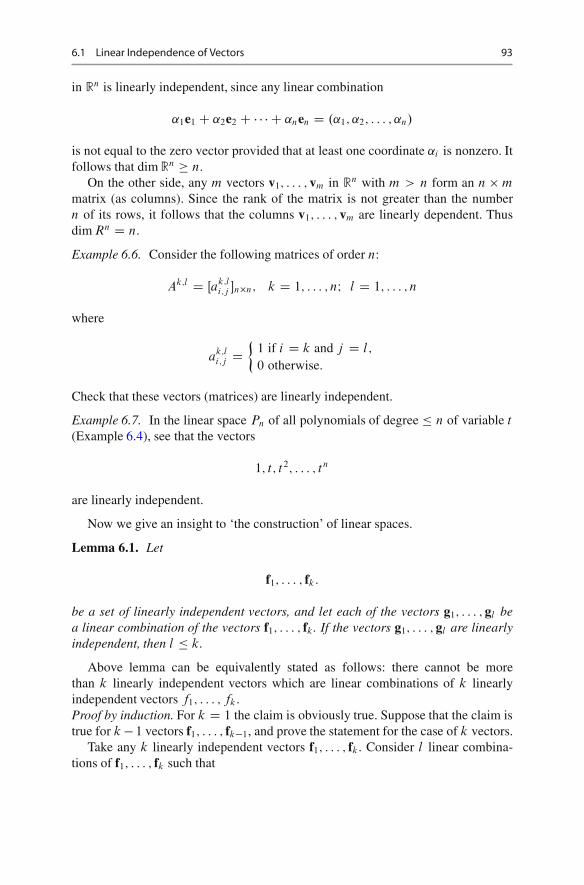
6.1 Linear Independence of Vectors 93
in Rn is linearly independent, since any linear combination
˛1e1 C ˛2e2 C � � � C ˛nen D .˛1; ˛2; : : : ; ˛n/
is not equal to the zero vector provided that at least one coordinate ˛i is nonzero. Itfollows that dim Rn � n.
On the other side, any m vectors v1; : : : ; vm in Rn with m > n form an n � m
matrix (as columns). Since the rank of the matrix is not greater than the numbern of its rows, it follows that the columns v1; : : : ; vm are linearly dependent. Thusdim Rn D n.
Example 6.6. Consider the following matrices of order n:
Ak;l D Œak;li;j �n�n; k D 1; : : : ; nI l D 1; : : : ; n
where
ak;li;j D
�1 if i D k and j D l;
0 otherwise:
Check that these vectors (matrices) are linearly independent.
Example 6.7. In the linear space Pn of all polynomials of degree � n of variable t
(Example 6.4), see that the vectors
1; t; t 2; : : : ; tn
are linearly independent.
Now we give an insight to ‘the construction’ of linear spaces.
Lemma 6.1. Let
f1; : : : ; fk:
be a set of linearly independent vectors, and let each of the vectors g1; : : : ; gl bea linear combination of the vectors f1; : : : ; fk . If the vectors g1; : : : ; gl are linearlyindependent, then l � k.
Above lemma can be equivalently stated as follows: there cannot be morethan k linearly independent vectors which are linear combinations of k linearlyindependent vectors f1; : : : ; fk .Proof by induction. For k D 1 the claim is obviously true. Suppose that the claim istrue for k� 1 vectors f1; : : : ; fk�1, and prove the statement for the case of k vectors.
Take any k linearly independent vectors f1; : : : ; fk. Consider l linear combina-tions of f1; : : : ; fk such that

94 6 Linear Spaces
g1 D ˛11f1 C � � � C ˛1kfk
g2 D ˛21f1 C � � � C ˛2kfk
:: : ::: : ::: : :
gl D ˛l1f1 C � � � C ˛lkfk:
Suppose that g1; : : : ; gl are linearly independent. We have to show that l � k. Thereare two cases to consider.
Case 1. If ˛jk D 0, for all j D 1; : : : ; l , then Lemma 6.1 is proved, since in thatcase l � k � 1 < k.
Case 2. Suppose there exists j 2 f1; : : : ; lg such that ˛jk ¤ 0. Without loss ofgenerality assume that ˛lk ¤ 0.
We will construct new l � 1 linearly independent vectors which in turn willbe linear combinations of f1; : : : ; fk�1. To do this, we solve for fk using the lastequality to get
fk D 1
˛lk
gl � ˛l1
˛lk
f1 � � � � � ˛l;k�1
˛lk
fk�1:
Now inserting fk into the above equalities and rearranging, we obtain
g1 � .˛1k=˛lk/gl D ˇ11f1 C � � � C ˇ1;k�1fk�1;
g2 � .˛2k=˛lk/gl D ˇ21f1 C � � � C ˇ2;k�1fk�1;
:: : ::: : ::: : :
gl�1 � .˛l�1;k=˛lk/gl D ˇl�1;1f1 C � � � C ˇl�1;k�1fk�1;
where ˇi;j D ˛i;j � ˛i;k˛l;j =˛l;k , for all i D 1; : : : ; l � 1 and j D 1; : : : ; k � 1.Then the vectors
g0i D gi � ˛ik
˛lk
gl ; i D 1; : : : ; l � 1;
are linear combinations of f1; : : : ; fk�1.If we can prove that g0
1; : : : ; g0l�1 are linearly independent, then by induction
assumption we will prove that l � 1 � k � 1, i.e. l � k.Suppose towards a contradiction that g0
1; : : : ; g0l�1 are linearly dependent, i.e.,
there are �1; : : : ; �l�1 such that
�1g01 C � � � C �l�1g0
l�1 D 0
or
�1.g1 � ˛1k
˛lk
gl /C : : : :C �l�1.gl�1 � ˛l�1;k
˛lk
gl / D 0
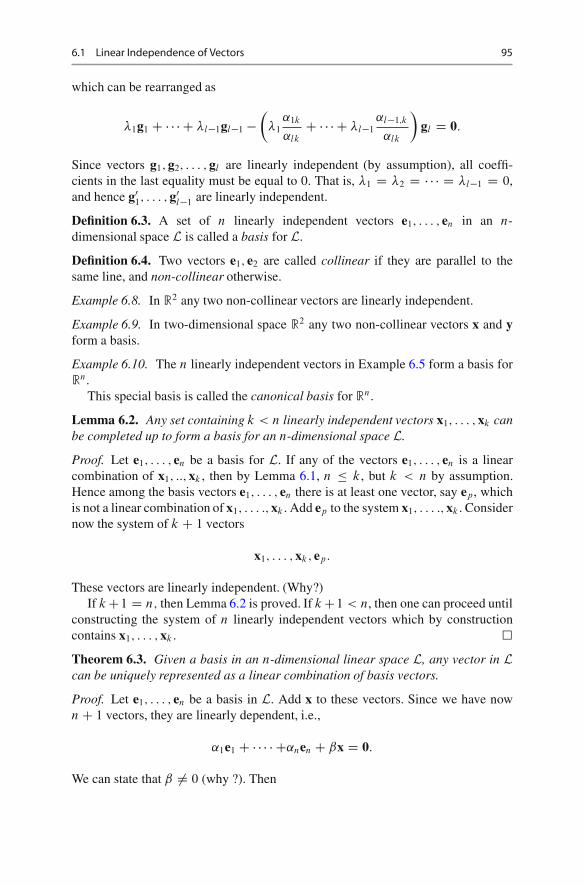
6.1 Linear Independence of Vectors 95
which can be rearranged as
�1g1 C � � � C �l�1gl�1 ��
�1
˛1k
˛lk
C � � � C �l�1
˛l�1;k
˛lk
�gl D 0:
Since vectors g1; g2; : : : ; gl are linearly independent (by assumption), all coeffi-cients in the last equality must be equal to 0. That is, �1 D �2 D � � � D �l�1 D 0,and hence g0
1; : : : ; g0l�1 are linearly independent.
Definition 6.3. A set of n linearly independent vectors e1; : : : ; en in an n-dimensional space L is called a basis for L.
Definition 6.4. Two vectors e1; e2 are called collinear if they are parallel to thesame line, and non-collinear otherwise.
Example 6.8. In R2 any two non-collinear vectors are linearly independent.
Example 6.9. In two-dimensional space R2 any two non-collinear vectors x and yform a basis.
Example 6.10. The n linearly independent vectors in Example 6.5 form a basis forRn.
This special basis is called the canonical basis for Rn.
Lemma 6.2. Any set containing k < n linearly independent vectors x1; : : : ; xk canbe completed up to form a basis for an n-dimensional space L.
Proof. Let e1; : : : ; en be a basis for L. If any of the vectors e1; : : : ; en is a linearcombination of x1; ::; xk , then by Lemma 6.1, n � k, but k < n by assumption.Hence among the basis vectors e1; : : : ; en there is at least one vector, say ep, whichis not a linear combination of x1; : : : :; xk . Add ep to the system x1; : : : :; xk . Considernow the system of k C 1 vectors
x1; : : : ; xk; ep:
These vectors are linearly independent. (Why?)If kC1 D n; then Lemma 6.2 is proved. If kC1 < n, then one can proceed until
constructing the system of n linearly independent vectors which by constructioncontains x1; : : : ; xk . �
Theorem 6.3. Given a basis in an n-dimensional linear space L, any vector in Lcan be uniquely represented as a linear combination of basis vectors.
Proof. Let e1; : : : ; en be a basis in L. Add x to these vectors. Since we have nownC 1 vectors, they are linearly dependent, i.e.,
˛1e1 C � � � � C˛nen C ˇx D 0:
We can state that ˇ ¤ 0 (why ?). Then
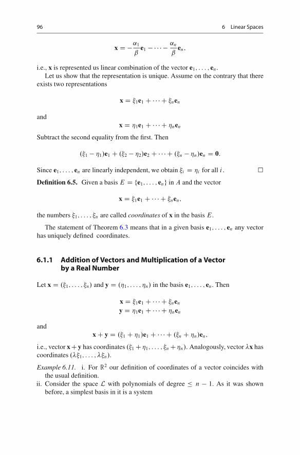
96 6 Linear Spaces
x D �˛1
ˇe1 � � � � � ˛n
ˇen;
i.e., x is represented us linear combination of the vector e1; : : : ; en.Let us show that the representation is unique. Assume on the contrary that there
exists two representations
x D �1e1 C � � � C �nen
andx D �1e1 C � � � C �nen
Subtract the second equality from the first. Then
.�1 � �1/e1 C .�2 � �2/e2 C � � � C .�n � �n/en D 0:
Since e1; : : : ; en are linearly independent, we obtain �i D �i for all i . �Definition 6.5. Given a basis E D fe1; : : : ; eng in A and the vector
x D �1e1 C � � � C �nen;
the numbers �1; : : : ; �n are called coordinates of x in the basis E:
The statement of Theorem 6.3 means that in a given basis e1; : : : ; en any vectorhas uniquely defined coordinates.
6.1.1 Addition of Vectors and Multiplication of a Vectorby a Real Number
Let x D .�1; : : : ; �n/ and y D .�1; : : : ; �n/ in the basis e1; : : : ; en. Then
x D �1e1 C � � � C �nen
y D �1e1 C � � � C �nen
andxC y D .�1 C �1/e1 C � � � C .�n C �n/en;
i.e., vector xCy has coordinates .�1C�1; : : : ; �nC�n/. Analogously, vector �x hascoordinates .��1; : : : ; ��n/.
Example 6.11. i. For R2 our definition of coordinates of a vector coincides withthe usual definition.
ii. Consider the space L with polynomials of degree � n � 1. As it was shownbefore, a simplest basis in it is a system

6.2 Isomorphism of Linear Spaces 97
e1 D 1; e2 D t; : : : ; en D tn�1:
Then any polynomial is represented as
P.t/ D a0tn�1 C a1tn�2 C � � � C an�1:
What are coordinates of the vector in this basis?Consider now another basis
e01 D 1; e0
2 D t � a; e03 D .t � a/2; : : : :; e0
n D .t � a/n�1:
Any polynomial P.t/, by Taylor expansion, can be represented as
P.t/ D P.a/C P 0.a/.t � a/C � � � C P .n�1/.a/
.n � 1/Š.t � a/n�1
What are the coordinates of P.t/ in this basis?
6.2 Isomorphism of Linear Spaces
Definition 6.6. Linear spaces L and L0 are called isomorphic if between vectorsx 2 L and x0 2 L0 there exists a one-to-one and onto correspondence x $ x0 suchthat(a) if x $ x0 ; y $ y0 then x C y $ x0 C y0I(b) �x $ �x0:
Lemma 6.4. If L and L0 are isomorphic then linearly independent vectors in L arelinearly independent in L0; and vice versa.
Proof. Exercise. utLemma 6.5. Two linear spaces L and L0 of different dimensions are not isomor-phic.
Proof. Exercise (use Lemma 6.4). utTheorem 6.2. All linear spaces of dimension n are isomorphic.
Proof. Let L, L0 be two n-dimensional spaces. Choose in L a basis e1; : : : ; en, andin L0 - a basis e0
1; : : : ; e0n.
For any vectorx D �1e1 C � � � C �nen (6.1)
construct the corresponding vector
x0 D �1e01 C � � � C �ne0
n: (6.2)

98 6 Linear Spaces
Note that coefficients are the same in both cases. This correspondence is a bijection(one-to-one and onto). Indeed, any x 2 L can be represented as in (6.1). Then, all�1; : : : ; �n and hence vector x0 are defined by x uniquely.
Change L and L0 in this reasoning and obtain a one-to-one and onto correspon-dence between L and L0.
Now, if x$ x0 ; y $ y0 then by construction xC y $ x0 C y0, and �x$ �x0.Hence, L and L0 are isomorphic. �
6.3 Subspaces
Subspace L0 of a linear space L is a subset of elements of L which itself is a linearspace with respect to operationsC and � defined in L.
In other words, if L0 � L, and C, and � are operations of addition andmultiplication by a real number defined in L, then all axioms I:.i/ � III:.i i/ aresatisfied for vectors in L0.
6.3.1 Examples of Subspaces
1. Null space and L itself.2. Consider R2. Then the set of all vectors which lie on same line going through
the origin is a linear subspace (Fig. 6.1).3. Consider L to be a set of n�tuples of real numbers:
x D .�1; : : : ; �n/:
The subset L0 of L such that
A D fx j .x D .�1; : : : ; �n/; �1 D 0/g
is a subspace of L:
Fig. 6.1 A one-dimensionalsubspace in R2
�
�
��
��
��
�
��
��
��
��
��
���
��
��
��
���
x
x C y
y

6.3 Subspaces 99
4. Let L be a space of all continuous functions on Œa; b� : Prove that the set of allpolynomials of degree less or equal to n � 1 is a subspace in L.
Since subspace of a linear space is a linear space itself, all notions introducedabove about linear independence, dimension, etc., are applied to the linear sub-spaces.
Hence, the dimension of a subspaceL0 of L can not be greater than the dimensionof L itself.
6.3.2 A Method of Constructing Subspaces
Choose in L vectors g1; g2; : : : ; gn: Then the set S of all linear combinations
˛1g1 C ˛2g2 C � � � C ˛ngn
of these vectors is a subspace of A.
Exercise 6.1. Prove the last statement above.
This subspace S is called a subspace spanned by the vectors g1; g2; : : : ; gn
(or simply span of these vectors) and is the smallest linear space which containsg1; g2; : : : ; gn: Notation: S D hg1; g2; : : : ; gni.Theorem 6.7. Subspace L0 spanned by linearly independent vectors e1; : : : ; ek isk-dimensional, and these vectors make a basis in L0.
Proof. Indeed, in L0 there is a set of linearly independent vectors, which aree1; : : : ; en themselves.
On the other hand, if x1; : : : ; xl are arbitrary linearly independent vectors in L0,they are linear combinations of e1; : : : ; ek; and by Lemma 6.1, l � k. Hence, L0 isk-dimensional subspace. �
6.3.3 One-Dimensional Subspaces
A basis of such a subspace consists of one vector, say, e1, and all subspace consistsof vectors ˛e1 , where ˛ is an arbitrary real number.
Consider a set of vectorsx D x0 C ˛e1;
where x0 , e1 are fixed, ˛ is an arbitrary real number. The set of such vectors can becalled a line in L.
6.3.4 Hyperplane
Analogously to a line in L, we can define a set of vectors
x D x0 C ˛e1 C ˇe2
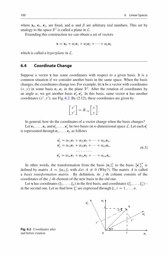
100 6 Linear Spaces
where x0, e1, e2, are fixed, and ˛ and ˇ are arbitrary real numbers. This set byanalogy to the space R3 is called a plane in L.
Extending this construction we can obtain a set of vectors
x D x0 C ˛1e1 C ˛2e2 C � � � C ˛kek
which is called a hyperplane in L.
6.4 Coordinate Change
Suppose a vector x has some coordinates with respect to a given basis. It is acommon situation if we consider another basis in the same space. When the basischanges, the coordinates change too. For example, let x be a vector with coordinates.x; y/ in some basis e1; e2 in the plane R2. After the rotation of coordinates byan angle ˛, we get another basis e0
1; e02. In this basis, same vector x has another
coordinates .x0; y0/, see Fig. 6.2. By (2.12), these coordinates are given by
�x0y0�D R�˛
�x
y
�:
In general, how do the coordinates of a vector change when the basis changes?Let e1; : : : ; en and e0
1; : : : ; e0n be two bases on n-dimensional space L. Let each e0
i
is represented through e1; : : : ; en as follows
e01 D ˛11e1 C ˛21e2 C � � � C ˛n1en;
e02 D ˛12e1 C ˛22e2 C � � � C ˛n2en;
: : : : : : : : : :
e0n D ˛1ne1 C ˛2ne2 C � � � C ˛nnen:
(6.3)
In other words, the transformation from the basis feign1 to the basis˚e0
i
�n
1is
defined by matrix A D k˛ikk, with det A ¤ 0 (Why?). The matrix A is calleda basis transformation matrix. By definition, its j -th column consists of thecoordinates of the j -th element of the new basis in the old one.
Let x has coordinates .�1; : : : ; �n/ in the first basis, and coordinates .� 01; : : : ; � 0
n/ –in the second one. Let us find how � 0
i are expressed through �i ; i D 1; : : : ; n.
Fig. 6.2 Coordinates afterand before rotation
�
�
��
��
���
x
�����������
0
e2
y
x e1
�
��
�
e0
2
y0x0
e0
1
˛
˛
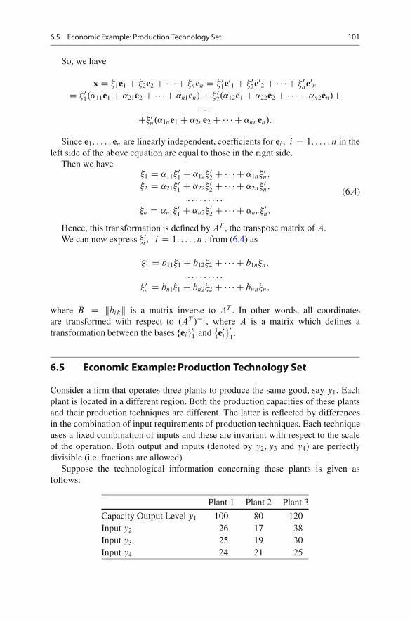
6.5 Economic Example: Production Technology Set 101
So, we have
x D �1e1 C �2e2 C � � � C �nen D � 01e0
1 C �02e0
2 C � � � C � 0ne0
n
D � 01.˛11e1 C ˛21e2 C � � � C ˛n1en/C � 0
2.˛12e1 C ˛22e2 C � � � C ˛n2en/C: : :
C� 0n.˛1ne1 C ˛2ne2 C � � � C ˛nnen/:
Since e1; : : : ; en are linearly independent, coefficients for ei , i D 1; : : : ; n in theleft side of the above equation are equal to those in the right side.
Then we have�1 D ˛11�
01 C ˛12� 0
2 C � � � C ˛1n� 0n;
�2 D ˛21�01 C ˛22� 0
2 C � � � C ˛2n� 0n;
: : : : : : : : :
�n D ˛n1� 01 C ˛n2�
02 C � � � C ˛nn� 0
n:
(6.4)
Hence, this transformation is defined by AT , the transpose matrix of A.We can now express � 0
i ; i D 1; : : : ; n , from (6.4) as
� 01 D b11�1 C b12�2 C � � � C b1n�n;
: : : : : : : : :
� 0n D bn1�1 C bn2�2 C � � � C bnn�n;
where B D kbikk is a matrix inverse to AT . In other words, all coordinatesare transformed with respect to .AT /�1, where A is a matrix which defines atransformation between the bases feign1 and
˚e0
i
�n
1.
6.5 Economic Example: Production Technology Set
Consider a firm that operates three plants to produce the same good, say y1. Eachplant is located in a different region. Both the production capacities of these plantsand their production techniques are different. The latter is reflected by differencesin the combination of input requirements of production techniques. Each techniqueuses a fixed combination of inputs and these are invariant with respect to the scaleof the operation. Both output and inputs (denoted by y2; y3 and y4) are perfectlydivisible (i.e. fractions are allowed)
Suppose the technological information concerning these plants is given asfollows:
Plant 1 Plant 2 Plant 3
Capacity Output Level y1 100 80 120Input y2 26 17 38Input y3 25 19 30Input y4 24 21 25
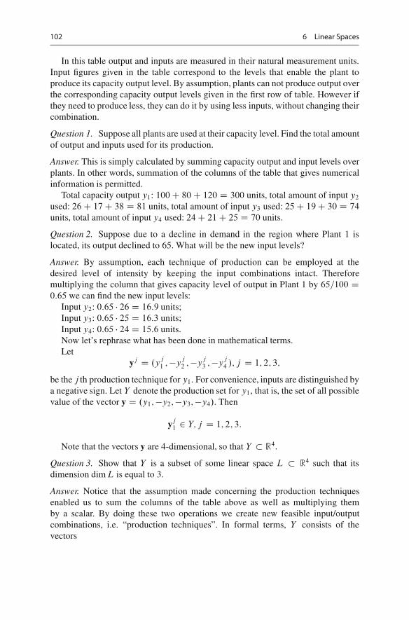
102 6 Linear Spaces
In this table output and inputs are measured in their natural measurement units.Input figures given in the table correspond to the levels that enable the plant toproduce its capacity output level. By assumption, plants can not produce output overthe corresponding capacity output levels given in the first row of table. However ifthey need to produce less, they can do it by using less inputs, without changing theircombination.
Question 1. Suppose all plants are used at their capacity level. Find the total amountof output and inputs used for its production.
Answer. This is simply calculated by summing capacity output and input levels overplants. In other words, summation of the columns of the table that gives numericalinformation is permitted.
Total capacity output y1: 100C 80C 120 D 300 units, total amount of input y2
used: 26C 17C 38 D 81 units, total amount of input y3 used: 25C 19C 30 D 74
units, total amount of input y4 used: 24C 21C 25 D 70 units.
Question 2. Suppose due to a decline in demand in the region where Plant 1 islocated, its output declined to 65. What will be the new input levels?
Answer. By assumption, each technique of production can be employed at thedesired level of intensity by keeping the input combinations intact. Thereforemultiplying the column that gives capacity level of output in Plant 1 by 65=100 D0:65 we can find the new input levels:
Input y2: 0:65 � 26 D 16:9 units;Input y3: 0:65 � 25 D 16:3 units;Input y4: 0:65 � 24 D 15:6 units.Now let’s rephrase what has been done in mathematical terms.Let
yj D .yj1 ;�y
j2 ;�y
j3 ;�y
j4 /; j D 1; 2; 3;
be the j th production technique for y1. For convenience, inputs are distinguished bya negative sign. Let Y denote the production set for y1, that is, the set of all possiblevalue of the vector y D .y1;�y2;�y3;�y4/. Then
yj1 2 Y; j D 1; 2; 3:
Note that the vectors y are 4-dimensional, so that Y � R4.
Question 3. Show that Y is a subset of some linear space L � R4 such that itsdimension dim L is equal to 3.
Answer. Notice that the assumption made concerning the production techniquesenabled us to sum the columns of the table above as well as multiplying themby a scalar. By doing these two operations we create new feasible input/outputcombinations, i.e. “production techniques”. In formal terms, Y consists of thevectors

6.5 Economic Example: Production Technology Set 103
3X
j D1
˛j yj � Y;
for ˛ � Œ0; 1�. Therefore, Y is a subset of the linear space L spanned by the vectorsy1; y2 and y3.
It remains to show that dim L D 3. By Theorem 6.7, it is sufficient to showthat three vectors y1; y2 and y3 are linearly independent. This means that the onlysolution of the equation
x1y1 C x2y2 C x3y3 D 0
is x1 D x2 D x3 D 0. Otherwise (i.e., if a solution with at least some nonzero valueexists), these vectors are dependent.
The vector equation above is equivalent to the matrix equation Ax D 0, where
x D2
4x1
x2
x3
3
5 and A D
2
664
100 80 120
�26 �17 �38
�25 �19 �30
�24 �21 �25
3
775
is a matrix formed by the vectors y1; y2 and y3 from the above table as the columns.By Theorem 5.6, we should prove that A is a matrix of full rank, that is, rank A D 3.Indeed, the minor determinant formed by the first three rows of A is
ˇˇˇˇˇ
100 80 120
�26 �17 �38
�25 �19 �30
ˇˇˇˇˇD 680 ¤ 0;
thus, rank A D 3. Therefore, dim L D 3.Interpretation of the result. In the above example each production technique was
represented by four figures. However, since the dimension of the technology set isonly three, which indicates that one of these figures is superfluous; it doesn’t add anyextra information to those supplied by the other three. This can be done by dividingall the entities in one column by the figure in the first row. The new figures will,then, give the input requirements per unit of output. These are called ‘input/outputcoefficients’. In this example the set of input/output coefficients is given as
2
40:260 0:213 0:317
0:250 0:276 0:250
0:240 0:263 0:208
3
5
Notice that this information is sufficient to calculate total input requirements at‘that particular output level’. The assumptions made so far, are not sufficient toensure that by using these coefficients one can get the amounts of inputs requiredto produce the specified level of output. In order to reach that generalization
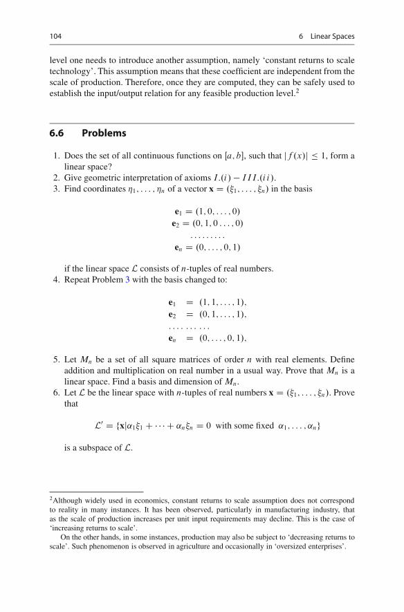
104 6 Linear Spaces
level one needs to introduce another assumption, namely ‘constant returns to scaletechnology’. This assumption means that these coefficient are independent from thescale of production. Therefore, once they are computed, they can be safely used toestablish the input/output relation for any feasible production level.2
6.6 Problems
1. Does the set of all continuous functions on Œa; b�, such that jf .x/j � 1, form alinear space?
2. Give geometric interpretation of axioms I:.i/ � III:.i i/.3. Find coordinates �1; : : : ; �n of a vector x D .�1; : : : ; �n/ in the basis
e1 D .1; 0; : : : ; 0/
e2 D .0; 1; 0 : : : ; 0/
: : : : : : : : :
en D .0; : : : ; 0; 1/
if the linear space L consists of n-tuples of real numbers.4. Repeat Problem 3 with the basis changed to:
e1 D .1; 1; : : : ; 1/;
e2 D .0; 1; : : : ; 1/;
: : : : : : : : : :
en D .0; : : : ; 0; 1/;
5. Let Mn be a set of all square matrices of order n with real elements. Defineaddition and multiplication on real number in a usual way. Prove that Mn is alinear space. Find a basis and dimension of Mn.
6. Let L be the linear space with n-tuples of real numbers x D .�1; : : : ; �n/. Provethat
L0 D fxj˛1�1 C � � � C ˛n�n D 0 with some fixed ˛1; : : : ; ˛ng
is a subspace of L.
2Although widely used in economics, constant returns to scale assumption does not correspondto reality in many instances. It has been observed, particularly in manufacturing industry, thatas the scale of production increases per unit input requirements may decline. This is the case of‘increasing returns to scale’.
On the other hands, in some instances, production may also be subject to ‘decreasing returns toscale’. Such phenomenon is observed in agriculture and occasionally in ‘oversized enterprises’.
6.6 Problems 105
7. Let f be a map from R2 to R2 given by f .x1; x2/ D .2x1; x2 � x1/. Check if f
is an isomorphism or not.8. Let f be a map from R3 to R3 given by f .x1; x2; x3/ D .x0
1; x02; x0
3/, where
2
4x0
1
x02
x03
3
5 D2
41 0 �1
2 5 10
0 �1 0
3
5
2
4x1
x2
x3
3
5 :
Check is f an isomorphism or not.9. Prove that the vector space M2 of 2 � 2 matrices and the vectors space P3 of
polynomials of degree at most 3 are isomorphic and give an explicit formula foran isomorphism from M2 to P3.
10. Show that the set S of symmetric matrices of order n is a subspace in Mn. Findthe dimension of S .
11. Let L0 be a subspace of L , and dimension of L0 be equal to the dimension of L.Then show that L D L0.
12. Let L be a space with n-tuples .�1; : : : ; �n/ of real numbers. Show that the setof vectors which meet the condition
˛1�1 C ˛2�2 C � � � C ˛n�n D 0;
where ˛1; : : : ; ˛n are real numbers not all equal to 0, forms a linear subspace ofL.
13. Let L1 and L2 be two subspaces of L such that
L1 \ L2 D 0:
Then show that dimL1 C dimL2 � dimL.14. Let L0 be a subspace spanned by vectors a; b; c; : : : . Show that dimL0 is equal
to the maximal number of linearly independent vectors in a; b; c; : : : .15. Find the coordinates of vector
x D .7; 14;�1; 2/
in the basise1 D .1; 2;�1; 1/;
e2 D .2; 3; 0;�1/;
e3 D .1; 2; 1; 3/;
e4 D .1; 3;�1; 0/:
Show that e1; : : : ; e4 make a basis.16. Let e1; e2; e3 and e0
1; e02; e0
3 be two bases for a linear space, and vectors e01; e0
2; e03
be defined trough e1; e2; e3 as:
106 6 Linear Spaces
e01 D 5e1 � e2 � 2e3;
e02 D 2e1 C 3e2;
e03 D �2e1 C e2 C 3e3:
Find the coordinates of the vector
x D �7e1 C 11e2 C 3e3
with respect to the basis e01; e0
2; e03.
17. Prove that each of the following two systems of vectors make a basis. Find thecoordinates in the basis e0 of a vector y if its coordinates in the basis e areye D .1; 2; 3; 4/.
e1 D .1; 1; 1; 1/
e2 D .1; 2; 1; 1/
e3 D .1; 1; 2; 1/
e4 D .1; 3; 2; 3/
e01 D .1; 0; 3; 3/
e02 D .�2;�3;�5;�4/
e03 D .2; 2; 5; 4/
e04 D .�2;�3;�4;�4/
18. Is any of these a linear subspace?(a) All vectors of n-dimensional space with integer coordinates?(b) All vectors on plane which lie either on axis x or on axis y?(c) All vectors of n-dimensional space with first coordinate equal to a given
number c?19. List all geometric types of linear subspaces of a 3-dimensional subspace.
20. Prove that L0 which consists of vectors with equal first and last coordinates is alinear subspace of n-dimensional space L D Rn. Find a basis and dimension ofthis subspace. Give an illustration for n D 2 and n D 3.
21. Find a basis and dimension of linear space spanned by the following vectors
a1 D .1; 1; 1; 1; 0/;
a2 D .1; 1;�1;�1;�1/;
a3 D .2; 2; 0; 0;�1/;
a4 D .1; 1; 5; 5; 2/;
a5 D .1;�1;�1; 0; 0/:
7Euclidean Spaces
In this chapter, we will analyse how various metric concepts, such as the length ofa vector, the angle between two vectors etc., are related to linear spaces. It is to benoted that one cannot directly define these concepts in linear spaces, since first a dotproduct for a given linear space should be defined.
7.1 General Definitions
Definition 7.1. Let L be a linear space over the real numbers. Consider the vectorsx; y; z and the scalars ˛ and ˇ. Then, a function .x; y/ which transforms a pair ofvectors x and y to real numbers is called a dot product1 if it satisfies the followingconditions:1. (symmetry) .x; y/ D .y; x/.
2. (bilinearity) .˛xC ˇy; z/ D ˛.x; z/C ˇ.y; z/.
3. (positivity) .x; x/ > 0 for all but one x.
Proposition 7.1. The only x 2 L such that .x; x/ D 0 is the null vector 0.
Proof. By condition 2, for null vector we have
.0; 0/ D .0 � 0; 0/ D 0.0; 0/ D 0:
It follows from condition 3 that for each x ¤ 0 we have .x; x/ > 0. �Definition 7.2. An n-dimensional linear space L over the real numbers with theinner-product function .x; y/ is called a Euclidean space.
1The dot product sometimes referred also as inner product and scalar product.
F. Aleskerov et al., Linear Algebra for Economists, Springer Texts in Businessand Economics, DOI 10.1007/978-3-642-20570-5 7,© Springer-Verlag Berlin Heidelberg 2011
107

108 7 Euclidean Spaces
Example 7.1. Consider the following spaces:(a) Let x D .�1; : : : ; �n/ be an n-tuple of real numbers, and y D .�1; : : : ; �n/.
Consider the dot product
.x; y/ DnX
iD1
�i �i :
Check that the corresponding space is Euclidean.(b) Let x D .�1; : : : ; �n/ and y D .�1; : : : ; �n/ be n-tuples in Rn. Consider some
matrix kaikkn�n and the function
.x; y/ DnX
iD1
nX
kD1
aik�i �i : (7.1)
Let us find some restrictions over the matrix kaikk so as to guarantee that theabove function is an inner-product. First note that condition 1 is met only ifkaikk is symmetric. Condition 2 is always satisfied. Let us check condition 3.We note that
.x; x/ DnX
iD1
nX
kD1
aik�i �i � 0 (7.2)
and .x; x/ D 0 if �1 D �2 D � � � D �n D 0. This property is called the positivedefiniteness of the polynomial
nX
iD1
nX
kD1
aik�i �i :
Thus, if kaikk is symmetric and the corresponding polynomial (it is also calledquadratic form) is positively defined, then the function defined by (7.1) is aninner-product.
(c) Consider the linear space defined by all continuous functions on Œa; b� � R.Note that the function
.f; g/ DZ b
a
f .x/g.x/dx
is an inner-product.
Definition 7.3. Given a Euclidean space E , the length of a vector x 2 E is denotedby jxj and defined as
jxj Dp
.x; x/:
Definition 7.4. Given a Euclidean space E , the distance between two vectors x; y 2E is denoted by d.x; y/ and defined as
d.x; y/ Dp
.x � y; x � y/:
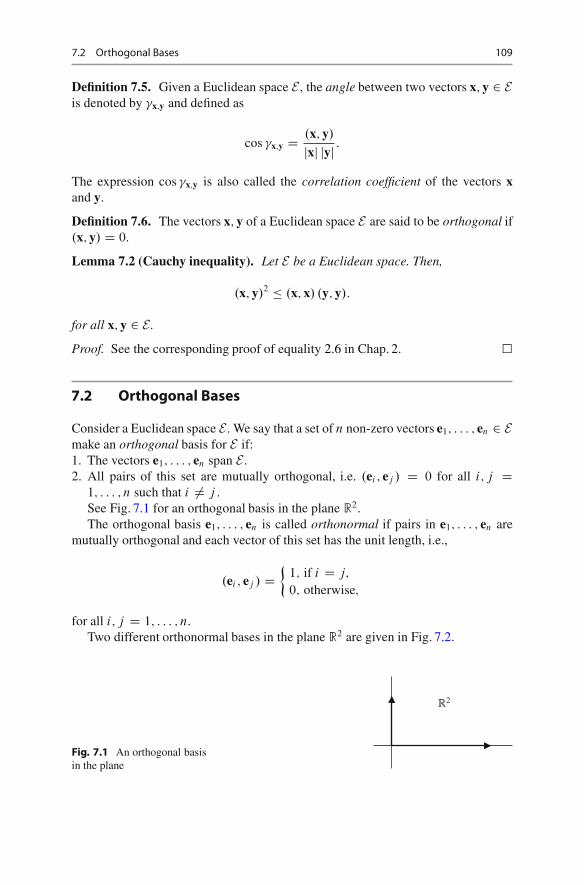
7.2 Orthogonal Bases 109
Definition 7.5. Given a Euclidean space E , the angle between two vectors x; y 2 Eis denoted by �x;y and defined as
cos �x;y D .x; y/
jxj jyj :
The expression cos �x;y is also called the correlation coefficient of the vectors xand y.
Definition 7.6. The vectors x; y of a Euclidean space E are said to be orthogonal if.x; y/ D 0.
Lemma 7.2 (Cauchy inequality). Let E be a Euclidean space. Then,
.x; y/2 � .x; x/ .y; y/:
for all x; y 2 E .
Proof. See the corresponding proof of equality 2.6 in Chap. 2. �
7.2 Orthogonal Bases
Consider a Euclidean space E . We say that a set of n non-zero vectors e1; : : : ; en 2 Emake an orthogonal basis for E if:1. The vectors e1; : : : ; en span E .2. All pairs of this set are mutually orthogonal, i.e. .ei ; ej / D 0 for all i; j D
1; : : : ; n such that i ¤ j .See Fig. 7.1 for an orthogonal basis in the plane R2.The orthogonal basis e1; : : : ; en is called orthonormal if pairs in e1; : : : ; en are
mutually orthogonal and each vector of this set has the unit length, i.e.,
.ei ; ej / D�
1; if i D j;
0; otherwise;
for all i; j D 1; : : : ; n.Two different orthonormal bases in the plane R2 are given in Fig. 7.2.
Fig. 7.1 An orthogonal basisin the plane
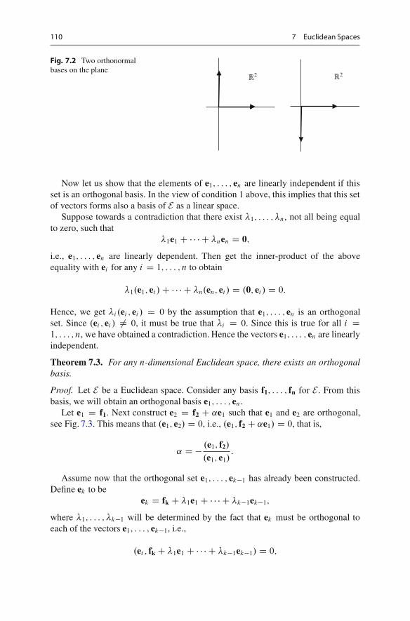
110 7 Euclidean Spaces
Fig. 7.2 Two orthonormalbases on the plane
Now let us show that the elements of e1; : : : ; en are linearly independent if thisset is an orthogonal basis. In the view of condition 1 above, this implies that this setof vectors forms also a basis of E as a linear space.
Suppose towards a contradiction that there exist �1; : : : ; �n, not all being equalto zero, such that
�1e1 C � � � C �nen D 0;
i.e., e1; : : : ; en are linearly dependent. Then get the inner-product of the aboveequality with ei for any i D 1; : : : ; n to obtain
�1.e1; ei /C � � � C �n.en; ei / D .0; ei / D 0:
Hence, we get �i.ei ; ei / D 0 by the assumption that e1; : : : ; en is an orthogonalset. Since .ei ; ei / ¤ 0, it must be true that �i D 0. Since this is true for all i D1; : : : ; n, we have obtained a contradiction. Hence the vectors e1; : : : ; en are linearlyindependent.
Theorem 7.3. For any n-dimensional Euclidean space, there exists an orthogonalbasis.
Proof. Let E be a Euclidean space. Consider any basis f1; : : : ; fn for E . From thisbasis, we will obtain an orthogonal basis e1; : : : ; en.
Let e1 D f1. Next construct e2 D f2 C ˛e1 such that e1 and e2 are orthogonal,see Fig. 7.3. This means that .e1; e2/ D 0, i.e., .e1; f2 C ˛e1/ D 0, that is,
˛ D � .e1; f2/
.e1; e1/:
Assume now that the orthogonal set e1; : : : ; ek�1 has already been constructed.Define ek to be
ek D fk C �1e1 C � � � C �k�1ek�1;
where �1; : : : ; �k�1 will be determined by the fact that ek must be orthogonal toeach of the vectors e1; : : : ; ek�1, i.e.,
.ei ; fk C �1e1 C � � � C �k�1ek�1/ D 0;
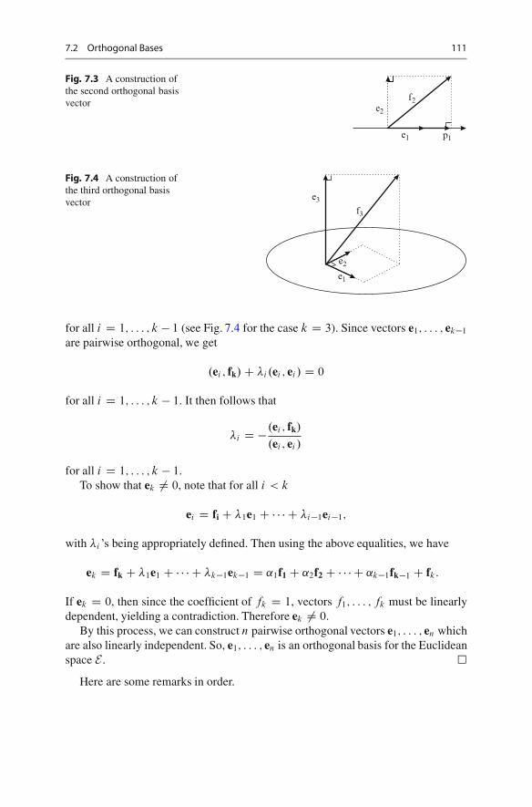
7.2 Orthogonal Bases 111
Fig. 7.3 A construction ofthe second orthogonal basisvector
e1
e2
f2
p1
Fig. 7.4 A construction ofthe third orthogonal basisvector
e1
e2
f3
e3
for all i D 1; : : : ; k � 1 (see Fig. 7.4 for the case k D 3). Since vectors e1; : : : ; ek�1
are pairwise orthogonal, we get
.ei ; fk/C �i.ei ; ei / D 0
for all i D 1; : : : ; k � 1. It then follows that
�i D � .ei ; fk/
.ei ; ei /
for all i D 1; : : : ; k � 1.To show that ek ¤ 0, note that for all i < k
ei D fi C �1e1 C � � � C �i�1ei�1;
with �i ’s being appropriately defined. Then using the above equalities, we have
ek D fk C �1e1 C � � � C �k�1ek�1 D ˛1f1 C ˛2f2 C � � � C ˛k�1fk�1 C fk:
If ek D 0, then since the coefficient of fk D 1, vectors f1; : : : ; fk must be linearlydependent, yielding a contradiction. Therefore ek ¤ 0.
By this process, we can construct n pairwise orthogonal vectors e1; : : : ; en whichare also linearly independent. So, e1; : : : ; en is an orthogonal basis for the Euclideanspace E . �
Here are some remarks in order.
112 7 Euclidean Spaces
Remark 7.1. The process of constructing an orthogonal basis from any given basisis called the Gram2–Schmidt3 orthogonalization process.
Remark 7.2. Given any orthogonal basis e1; : : : ; en, the set of vectorse1=je1j; : : : ; en=jenj form an orthonormal basis.
Example 7.2. Let L be a subspace in R4 spanned by three vectors f1 D .1; 1; 0; 1/,f2 D .3; 1; 1;�1/ and f3 D .�1; 2;�3; 2/. Let us construct an orthogonal andorthonormal bases of V .
Note that the vector f1; f2 and f3 form a basis of L (since these vectors arelinearly independent), so that we can apply the Gram–Schmidt procedure. First, letus construct an orthogonal basis. Let e1 D f1 D .1; 1; 0; 1/ be its first element. Forthe second element, we put e2 D f2 C ˛21e1, where
˛21 D � .e1; f2/
.e1; e1/D �3
3D �1;
so that e2 D f2 � e1 D .2; 0; 1;�2/. To construct the third element of the basis, weput
e3 D f3 C ˛31e1 C ˛32e2;
where
˛31 D � .e1; f3/
.e1; e1/D �3
3D �1 and ˛32 D � .e2; f3/
.e2; e2/D ��9
9D 1:
Thus e3 D f3 � e1 C e2 D .0; 1;�2;�1/. Now, the vectors e1; e2 and e3 form anorthogonal basis for L.
By Remark 7.2, the vectors
e01D
1
je1je1D 1p3
e1D�
1p3
;1p3
; 0;1p3
�; e0
2D1
je2je2D 1
3e2D
�2
3; 0;
1
3;�2
3
�
and
e03 D
1
je3je3 D 1p6
e3 D�
0;1p6
;� 1p3
;� 1p6
�
form an orthonormal basis of L.
2Jorgen Pedersen Gram (1850–1916) was a Danish mathematician who was famous because ofhis works both in pure mathematics (algebra and number theory) and applications (such as amathematical model of forest management).3Erhard Schmidt (1876–1959) was an Estonia born German mathematician, one of originators offunctional analysis.

7.2 Orthogonal Bases 113
Remark 7.3. For any order of the basis vectors f1; : : : ; fn, we may get a differentorthogonal basis by the Gram-Schmidt orthogonalization process. So, it is obviousthat orthogonal bases for any Euclidean space are not necessarily unique.
Let L be a Euclidean space, and e1; : : : ; en be an orthonormal basis for it. Letx; y 2 L be two vectors such that
x D �1e1 C � � � C �nen;
y D �1e1 C � � � C �nen:
Let us find the inner-product
.x; y/ D .�1e1 C � � � C �nen; �1e1 C � � � C �nen/
in terms of the coordinates of these two vectors. From the fact
.ei ; ej / D�
1 if i D j
0 otherwise
it follows that
.x; y/ DnX
iD1
�i �i ;
i.e., the inner-product of two vectors that are defined with respect to an orthonormalbasis is equal to the sum of the products of their coordinates.
Now, let us express any vector x 2 L with respect to the orthonormal basise1; : : : ; en. That is, we want to find �i for all i D 1; : : : ; n in the expression
x D �1e1 C � � � C �nen:
Multiplying x by ei , we get
.x; ei / D �1.e1; ei /C � � � C �n.en; ei / D �i .ei ; ei / D �i :
Hence we have�i D .x; ei /
for all i D 1; : : : ; n.The vector .x; ei /ei , where ei is a vector of unit length, is called the projection
of x on ei . Then, the coordinates of any vector with respect to an orthonormal basiscan be regarded as the lengths of projections of the vector on each basis vector.
Definition 7.7. Let L be a Euclidean space. Then a vector x 2 L is calledorthogonal to a subspace B of L if it is orthogonal to each vector y 2 B .
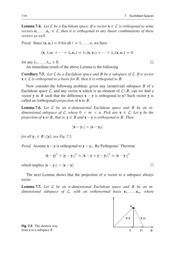
114 7 Euclidean Spaces
Lemma 7.4. Let L be a Euclidean space. If a vector x 2 L is orthogonal to somevectors e1; : : : ; en 2 L, then it is orthogonal to any linear combinations of thesevectors as well.
Proof. Since .x; ei / D 0 for all i D 1; : : : ; n, we have
.x; �1e1 C � � � C �nen/ D �1.x; e1/C � � � C �n.x; en/ D 0;
for any �1; : : : ; �m 2 R. �An immediate result of the above Lemma is the following
Corollary 7.5. Let L be a Euclidean space and B be a subspace of L. If a vectorx 2 L is orthogonal to a basis for B , then it is orthogonal to B .
Now consider the following problem: given any (nontrivial) subspace B of aEuclidean space L, and any vector x which is an element of L\B , can we find avector y in B such that the difference x � y is orthogonal to x? Such vector y iscalled an (orthogonal) projection of x to B .
Lemma 7.6. Let L be an n-dimensional Euclidean space and B be an m-dimensional subspace of L, where 0 < m < n. Pick any x 2 L. Let y be theprojection of x to B , that is, y 2 B and x � y is orthogonal to B . Then
jx � y1j > jx � y0j
for all y1 2 B\fyg, see Fig. 7.5.
Proof. Assume x � y is orthogonal to y � y1: By Pythagoras’ Theorem
jx � yj2 C jy � y1j2 D jx � yC y � y1j2 D jx � y1j2
which implies jx � y1j > jx � yj. �
The next Lemma shows that the projection of a vector to a subspace alwaysexists.
Lemma 7.7. Let L be an n-dimensional Euclidean space and B be an m-dimensional subspace of L, with an orthonormal basis e1; : : : ; em, where
Fig. 7.5 The shortest wayfrom x to a subspace B
�
�
��
��
��
�
�
���
��
��
B
x
y y1
x-y1x-y

7.2 Orthogonal Bases 115
Fig. 7.6 The projectionon a line
e1
e2
x
y=(x,e1)e1
Fig. 7.7 The projectionon a plane
�
��
�
��
��
��
��
���
��
��
��
��
��
��
e1
e2
B
x
y
c1
c2
x-y
0 < m < n. Then the orthogonal projection of any vector x 2 L\B on B is
y0 D c1e1 C � � � C cmem
where ci D .x; ei / for all i D 1; : : : ; m.
The statement of Lemma 7.7 is illustrated in Fig. 7.6 for the case n D 2; m D 1 andin Fig. 7.7 for the case n D 3; m D 2.
Proof. Let y D c1e1 C � � � C cmem be the orthogonal projection of x 2 L\B on B .Then x� y is orthogonal to B , i.e., .x� y; ei / D 0, implying .x; ei / D .y; ei / for alli D 1; : : : ; m. It follows that
.x; ei / D c1.e1; ei /C � � � C cm.em; ei / D ci .ei ; ei / D ci ; i D 1; : : : ; m:
�The distance between a vector x and a subspace B in a Euclidean space L is the
minimal length of a vector of the form x � y, where y 2 B , that is, the distance
d.x; B/ D miny2Bfjx � yjg:
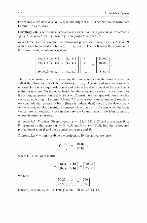
116 7 Euclidean Spaces
For example, we have d.x; B/ D 0 if and only if x 2 B . Then we can re-formulateLemma 7.6 as follows
Corollary 7.8. The distance between a vector x and a subspace B in a Euclideanspace L is equal to jx � yj, where y is the projection of x to B .
Remark 7.4. Let us now find the orthogonal projection of any vector x 2 L on B
with respect to an arbitrary basis e1; : : : ; em for B . Then following the argument inthe above proof, we obtain a system
2
664
.e1; e1/ .e2; e1/ : : : .em; e1/
.e1; e2/ .e2; e2/ : : : .em; e2/
: : : : : : : : : : : : :
.e1; em/ .e2; em/ : : : .em; em/
3
775
2
664
c1
c2
: : : :
cm
3
775 D
2
664
.x; e1/
.x; e2/
: : : :
.x; em/
3
775 :
The m � m matrix above, containing the inner-product of the basis vectors, iscalled the Gram matrix of the vectors e1; : : : ; em. A system of m equations withm variables has a unique solution if and only if the determinant of the coefficientmatrix is nonzero. On the other hand, the above equation system, when describesthe orthogonal projection of a vector x on B , must have a unique solution, since thevector y, according to Lemmas 7.6 and 7.7, always exists and is unique. From herewe conclude that given any basis (linearly independent) vectors, the determinantof the associated Gram matrix is nonzero. Note that this is obvious when the basisvectors are orthonormal, since in that case the Gram matrix is the identity matrixwhose determinant is one.
Example 7.3. Problem. Given a vector x D .25; 0; 25/ 2 R3 and a subspace B �R3 spanned by the vectors a D .3; 4; 5/ and b D .�4; 3; 5/, find the orthogonalprojection of x on B and the distance between x and B .
Solution. Let y D c1aC c2b be the projection. By the above, we have
G
�c1
c2
�D�
.x; a/
.x; b/
�;
where G is the Gram matrix,
G D�
.a; a/ .a; b/
.b; a/ .b; b/
�D�
50 25
25 50
�:
We have �50 25
25 50
� �c1
c2
�D�
200
25
�;
hence c1 D 5 and c2 D �2. Thus y D 5a� 2b D .23; 14; 15/.
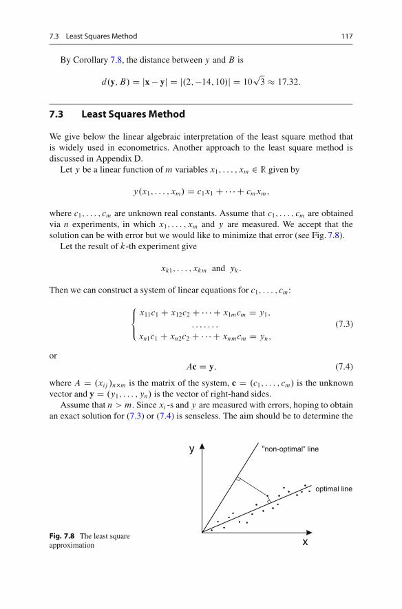
7.3 Least Squares Method 117
By Corollary 7.8, the distance between y and B is
d.y; B/ D jx � yj D j.2;�14; 10/j D 10p
3 � 17:32:
7.3 Least Squares Method
We give below the linear algebraic interpretation of the least square method thatis widely used in econometrics. Another approach to the least square method isdiscussed in Appendix D.
Let y be a linear function of m variables x1; : : : ; xm 2 R given by
y.x1; : : : ; xm/ D c1x1 C � � � C cmxm;
where c1; : : : ; cm are unknown real constants. Assume that c1; : : : ; cm are obtainedvia n experiments, in which x1; : : : ; xm and y are measured. We accept that thesolution can be with error but we would like to minimize that error (see Fig. 7.8).
Let the result of k-th experiment give
xk1; : : : ; xkm and yk:
Then we can construct a system of linear equations for c1; : : : ; cm:
8<
:
x11c1 C x12c2 C � � � C x1mcm D y1;
: : : : : : :
xn1c1 C xn2c2 C � � � C xnmcm D yn;
(7.3)
orAc D y; (7.4)
where A D .xij /n�m is the matrix of the system, c D .c1; : : : ; cm/ is the unknownvector and y D .y1; : : : ; yn/ is the vector of right-hand sides.
Assume that n > m. Since xi -s and y are measured with errors, hoping to obtainan exact solution for (7.3) or (7.4) is senseless. The aim should be to determine the
Fig. 7.8 The least squareapproximation x
y
optimal line
“non-optimal” line
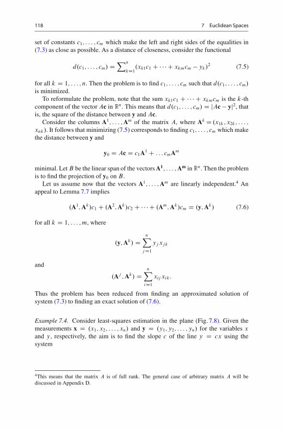
118 7 Euclidean Spaces
set of constants c1; : : : ; cm which make the left and right sides of the equalities in(7.3) as close as possible. As a distance of closeness, consider the functional
d.c1; : : : ; cm/ DXn
kD1.xk1c1 C � � � C xkmcm � yk/2 (7.5)
for all k D 1; : : : ; n. Then the problem is to find c1; : : : ; cm such that d.c1; : : : ; cm/
is minimized.To reformulate the problem, note that the sum xk1c1 C � � � C xkmcm is the k-th
component of the vector Ac in Rn. This means that d.c1; : : : ; cm/ D jAc � yj2, thatis, the square of the distance between y and Ac.
Consider the columns A1; : : : ; Am of the matrix A, where AkD .x1k ; x2k; : : : ;
xnk/. It follows that minimizing (7.5) corresponds to finding c1; : : : ; cm which makethe distance between y and
y0 D Ac D c1A1 C : : : cmAm
minimal. Let B be the linear span of the vectors A1; : : : ; Am in Rn. Then the problemis to find the projection of y0 on B .
Let us assume now that the vectors A1; : : : ; Am are linearly independent.4 Anappeal to Lemma 7.7 implies
.A1; Ak/c1 C .A2; Ak/c2 C � � � C .Am; Ak/cm D .y; Ak/ (7.6)
for all k D 1; : : : ; m, where
.y; Ak/ DnX
j D1
yj xjk
and
.Aj ; Ak/ DnX
iD1
xij xik:
Thus the problem has been reduced from finding an approximated solution ofsystem (7.3) to finding an exact solution of (7.6).
Example 7.4. Consider least-squares estimation in the plane (Fig. 7.8). Given themeasurements x D .x1; x2; : : : ; xn/ and y D .y1; y2; : : : ; yn/ for the variables x
and y, respectively, the aim is to find the slope c of the line y D cx using thesystem
4This means that the matrix A is of full rank. The general case of arbitrary matrix A will bediscussed in Appendix D.

7.4 Isomorphism of Euclidean Spaces 119
8ˆ<
ˆ:
y1 D cx1;
y2 D cx2;
: : : : : : : : :
yn D cxn:
Using (7.6) we obtain
c D .x; y/
.x; x/DPn
kD1 xkykPnkD1 x2
k
:
For n D 4, .x1; x2; x3; x4/ D .1; 2; 3; 4/ and .y1; y2; y3; y4/ D .2; 3; 4; 10/,check that c D 2.
7.4 Isomorphism of Euclidean Spaces
Definition 7.8. Any two Euclidean spaces L and L0 are said to be isomorphic ifthey are isomorphic as linear spaces and if .x; y/ D .x0; y0/ whenever
L 3 x ! x0 2 L0;L 3 y ! y0 2 L0;
Theorem 7.9. Any two n-dimensional Euclidean spaces are isomorphic.
Proof. It is sufficient to prove that any n-dimensional Euclidean space L isisomorphic to Rn.
Isomorphism of L and L0 as linear spaces is obvious, so we will prove the rest.Given any orthonormal basis e1; : : : en in L, let the dot product of two vectors
x D �1e1 C : : : :C �nen and y D �1e1 C � � � C �nen in L be defined as
.x; y/ D �1�1 C � � � C �n�n:
Now consider any n-dimensional Euclidean space L. Choose for it an orthonormalbasis e1; : : : en. (It must exist, why?) For any two vectors x0 D �1e1C� � �C �nen andy0 D �1e1C � � �C �nen in L, pick the vectors x D .�1; : : : ; �n/ and y D .�1; : : : ; �n/
in Rn, and vice versa. (Note that we use the canonical basis for Rn.)Then we have
.x0; y0/ D �1�1 C � � � C �n�n:
On the other hand,.x; y/ D �1�1 C � � � C �n�n:
Thus,.x0; y0/ D .x; y/;
completing the proof. �

120 7 Euclidean Spaces
7.5 Problems
1. Check whether the function defined by equation (7.1) is an inner product for thematrices:
(a)
�1 1
1 2
�; (b)
�0 1
1 0
�:
2. Consider any two vectors
x D .�1; : : : ; �n/;
y D .�1; : : : ; �n/
in Rn. Check whether any of the following functions is an inner-product:
(a) .x; y/ DPnj D1 j�i j j�i j; (b) .x; y/ DPn
j D1 �2i �2
i .3. Consider the basis given by the vectors
f1 D .1; 1; : : : ; 1; 1/;
f2 D .0; 1; : : : ; 1; 1/;
:: : :
:: : :
:: : :
fn D .0; 0; : : : ; 0; 1/:
Is this basis orthogonal? If not, construct an orthogonal basis using Gram-Schmidt process. For this basis, find the associated orthonormal basis.
4. Prove that for any Euclidean space L, any vectors x; y 2 L and � 2 R, if x D �ythen
jxj D j�j jyj :5. Let L1 and L2 be linear subspaces of the Euclidean space R4 such that
dimL1 D dimL2:
Prove that there exists a non-zero vector x 2 L2 which is orthogonal to L1.6. Check whether the following vectors are orthogonal and complete them up to a
basis for R4.(a) f1 D .1;�2; 2;�3/ and f2 D .2;�3; 2; 4/.(b) f1 D .1; 1; 1; 2/ and f1 D .1; 2; 3;�3/.
7. Consider the Euclidean space R4. Find the angles between the line �1 D �2 D�3 D �4 and the vectors e1 D .1; 0; 0; 0/, e2 D .0; 1; 0; 0/, e3 D .0; 0; 1; 0/ ande4 D .0; 0; 0; 1/.
8. Let L1 and L2 be two orthogonal subspaces of a Euclidean space L. Prove thatL1 \ L2 D 0.
7.5 Problems 121
9. Given the space of polynomials of degree at most n, and any two polynomialsP and Q in this space, consider the mapping
.P.t/; Q.t// DZ b
a
P.t/Q.t/dt:
(a) Check that the above mapping is an inner-product.
(b) Find the distance between the polynomials P.t/ D 3t2 C 6 and Q.t/ D2t2 C t C 1 according to the above inner-product.
10. Using Gramm-Shmidt orthogonalization process construct an orthonormalbasis from the vectors
f1 D .2; 1; 3;�1/;
f2 D .7; 4; 3;�3/;
f3 D .1; 1;�6; 0/;
f4 D .5; 7; 7; 8/:
11. Find the distance between the vector x D .4;�1;�3; 4/ and a linear subspacedefined by the vectors
e1 D .1; 1; 1; 1/;
e2 D .1; 2; 2;�1/;
e3 D .1; 0; 0; 3/:
12. Let L be a subspace defined by the system of linear equations
8<
:
2x1 C x2 C x3 C 3x4 D 0;
3x1 C 2x2 C 2x3 C x4 D 0;
x1 C 2x2 C 2x3 � 9x4 D 0:
Consider the vector x D .7;�4;�1; 2/. Find the orthogonal projection (callit y) of x on L. Find also x � y.
13. (a) Find the distance between the vector x D .4; 2;�5; 1/ and the linear spaceL defined by the system
�2x1 � 2x2 C x3 C 2x4 D 9;
2x1 � 4x2 C 2x3 C 3x4 D 12:
(b) Find the distance between the vector x D .2; 4;�4; 2/ and the linear spaceL defined by the system
�x1 C 2x2 C x3 � x4 D 1;
x1 C 3x2 C x3 � 3x4 D 2:
14. Find the least square approximation for the function y.x1; x2/ D c1x1 C c2x2,if its three measurements give y.0; 1/ D 3; y.1; 2/ D 8; y.�1; 0/ D 0.
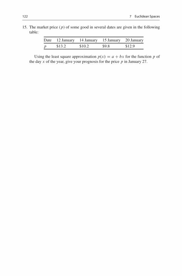
122 7 Euclidean Spaces
15. The market price (p) of some good in several dates are given in the followingtable:
Date 12 January 14 January 15 January 20 January
p $13.2 $10.2 $9.8 $12.9
Using the least square approximation p.x/ D a C bx for the function p ofthe day x of the year, give your prognosis for the price p in January 27.
8Linear Transformations
We will begin with a general definition of transformations and then study lineartransformations.1
Definition 8.1. A mapping F from a set S to another set S 0 is a relation which, toevery element x of S , associates an element y of S 0. This mapping is denoted byF W S ! S 0.
If x is an element of S , then y D F.x/ is called the image of x under F .Analogously, the set
B D fF.x/ j x 2 Sgis called the image of S (or full image). Naturally, B � S 0. In the same way, forW � S , the set
F.W / D fF.x/ j x 2 W gis called the image of W under F .
Example 8.1. (a) Let S D S 0 D R and F.x/ D x2. Then the image of S is the setof all non-negative numbers.(b) Let L W R3 ! R be a mapping such that for all x 2 R3, L.x/ D .a; x/, where
a D .3; 2; 1/.
Given any set S , the identity mapping IS is defined such that IS.x/ D x for allx 2 S .
Definition 8.2. A mapping F W S ! S 0 is said to have the inverse if there exists amapping G W S 0 ! S such that
G � F D IS and F �G D IS 0 ;
that is, G.F.x// D x and F.G.y// D y for all x 2 S; y 2 S 0.
1One may use the terms linear mapping, linear map, homomorphism and linear transformationinterchangeably.
F. Aleskerov et al., Linear Algebra for Economists, Springer Texts in Businessand Economics, DOI 10.1007/978-3-642-20570-5 8,© Springer-Verlag Berlin Heidelberg 2011
123
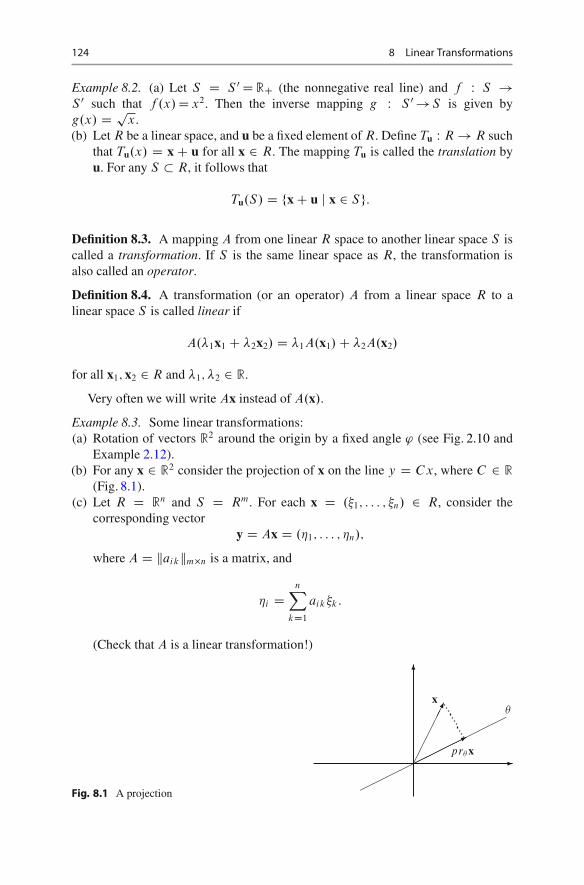
124 8 Linear Transformations
Example 8.2. (a) Let S D S 0DRC (the nonnegative real line) and f W S !S 0 such that f .x/D x2. Then the inverse mapping g W S 0!S is given byg.x/ D px.(b) Let R be a linear space, and u be a fixed element of R. Define Tu W R! R such
that Tu.x/ D xC u for all x 2 R. The mapping Tu is called the translation byu. For any S � R, it follows that
Tu.S/ D fxC u j x 2 Sg:
Definition 8.3. A mapping A from one linear R space to another linear space S iscalled a transformation. If S is the same linear space as R, the transformation isalso called an operator.
Definition 8.4. A transformation (or an operator) A from a linear space R to alinear space S is called linear if
A.�1x1 C �2x2/ D �1A.x1/C �2A.x2/
for all x1; x2 2 R and �1; �2 2 R.
Very often we will write Ax instead of A.x/.
Example 8.3. Some linear transformations:(a) Rotation of vectors R2 around the origin by a fixed angle ' (see Fig. 2.10 and
Example 2.12).(b) For any x 2 R2 consider the projection of x on the line y D Cx, where C 2 R
(Fig. 8.1).(c) Let R D Rn and S D Rm. For each x D .�1; : : : ; �n/ 2 R, consider the
corresponding vectory D Ax D .�1; : : : ; �n/;
where A D kaikkm�n is a matrix, and
�i DnX
kD1
aik�k:
(Check that A is a linear transformation!)
Fig. 8.1 A projection
�
�
�������
�����
������
����
�
pr� x
x
8 Linear Transformations 125
(d) Let R be the linear space of all polynomials (over real numbers) having thedegree at most n � 1. Define A such that
A.P.t// D P 0.t/;
where P 0.t/ is the derivative of polynomial P.t/ with respect to t . Then A is alinear operator on R, since
A.�1P.t/C �2Q.t// D .�1P.t/C �2Q.t//0
D �1P 0.t/C �2Q0.t/
D �1A.P.t//C �2A.Q.t//:
for all P; Q 2 R and �1; �2 2 R.(e) Let R be the linear space of all continuous functions f .t/ on Œ0; 1�. Let
A.f .t// DZ 1
0
f .r/dr:
Then A is a linear transformation from R to a one-dimensional vector space R,because
A.�1f1 C �2f2/ DZ 1
0
Œ�1f1.r/C �2f2.r/�dr D �1A.f1/C �2A.f2/
for all f1; f2 2 R and �1; �2 2 R.Two special transformations are the following– Identity operator (I ): For all linear spaces R and x 2 R, I x D x.– Null operator (‚): For all linear spaces R and x 2 R, ‚x D 0.
Theorem 8.1. Let R be an n-dimensional linear space, and let e1; : : : ; en be a basisfor R. Then for any set of vectors g1; : : : ; gn of another linear space S there existsa unique linear transformation A from R to S such that
Aei D gi ; for all i D 1; : : : ; n:
Proof. Let us first prove that for any vector g1; : : : ; gn there exists a lineartransformation A such that
Aei D gi for all i D 1; : : : ; n:
For eachx D �1e1 C � � � C �nen 2 R
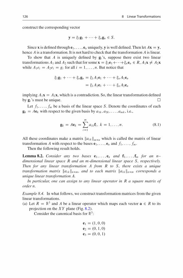
126 8 Linear Transformations
construct the corresponding vector
y D �1g1 C � � � C �ngn 2 S:
Since x is defined through e1; : : : ; en uniquely, y is well defined. Then let Ax D y,hence A is a transformation. It is not hard to check that the transformation A is linear.
To show that A is uniquely defined by gi ’s, suppose there exist two lineartransformations A1 and A2 such that for some x D �1e1C� � �C�nen 2 R, A1x ¤ A2xwhile A1ei D A2ei D gi for all i D 1; : : : ; n. But notice that
�1g1 C � � � C �ngn D �1A1e1 C � � � C �nA1en
D �1A2e1 C � � � C �nA2en
implying A1x D A2x, which is a contradiction. So, the linear transformation definedby gi ’s must be unique. �
Let f1; : : : ; fm be a basis of the linear space S . Denote the coordinates of eachgk D Aek with respect to the given basis by a1k; a2k ; : : : ; amk , i.e.,
gk D Aek DmX
iD1
aikfi ; k D 1; : : : ; n: (8.1)
All these coordinates make a matrix kaikkm�n which is called the matrix of lineartransformation A with respect to the bases e1; : : : ; en and f1; : : : ; fm.
Then the following result holds.
Lemma 8.2. Consider any two bases e1; : : : ; en and f1; : : : ; fm for an n–dimensional linear space R and an m-dimensional linear space S , respectively.Then for any linear transformation A from R to S , there exists a uniquetransformation matrix kaikkn�m, and to each matrix kaikkn�m corresponds aunique linear transformation A.
In particular, one can assign to any linear operator in R a square matrix oforder n.
Example 8.4. In what follows, we construct transformation matrices from the givenlinear transformations.(a) Let R D R3 and A be a linear operator which maps each vector a 2 R to its
projection on the XY plane (Fig. 8.2).Consider the canonical basis for R3:
e1 D .1; 0; 0/
e2 D .0; 1; 0/
e3 D .0; 0; 1/
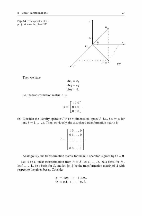
8 Linear Transformations 127
Fig. 8.2 The operator of aprojection on the plane XY
��
�
��
��
��
�
��
�
��
��
���
��
��
��
e1
e2
e3
x
y
z
prXY aXY
a
Then we haveAe1 D e1
Ae2 D e2
Ae3 D 0:
So, the transformation matrix A is
A D2
41 0 0
0 1 0
0 0 0
3
5 :
(b) Consider the identify operator I in an n dimensional space R, i.e., I ei D ei forany i D 1; : : : ; n. Then, obviously, the associated transformation matrix is
I D
2
666664
1 0 : : : 0
0 1 : : : 0: : : :: : : :: : : :
0 0 : : : 1
3
777775
:
Analogously, the transformation matrix for the null operator is given by ‚ D 0.
Let A be a linear transformation from R to S , let e1; : : : ; en be a basis for R ,let f1; : : : ; fm be a basis for S , and let kaikk be the transformation matrix of A withrespect to the given bases. Consider
x D �1e1 C � � � C �nen;
Ax D �1f1 C � � � C �mfm:

128 8 Linear Transformations
Let us find how the coordinates of Ax can be expressed through those of x. Observethat
Ax D A.�1e1 C � � � C �nen/
D �1.a11f1 C a21f2 C � � � C am1fm/C �2.a12f1 C a22e2 C � � � C am2fm/
C � � � C �n.a1nf1 C a2nf2 C � � � C amnfm/
D .a11�1 C a12�2 C � � � C a1n�n/f1 C .a21�1 C a22�2 C � � � C a2n�n/f2
C � � � C .am1�1 C am2�2 C � � � C amn�n/em:
Then
�i DnX
kD1
aik�k ; i D 1; : : : ; n:
The last equality may be simply re-written in matrix from. Let � be the columnvector of coordinates of the vector x and let � be the column vector of coordinatesof the vector Ax in the given bases, that is,
� D
0
B@
�1
:::
�n
1
CA and � D
0
B@
�1
:::
�m
1
CA
Then� D kaikk �:
Therefore, we have
Theorem 8.3. Given a linear transformation A from a linear space R to anotherlinear space S and some bases in R and S , let � be a column vector of coordinatesof a vector x 2 R, let � be the column vector of coordinates of the vector Ax 2 S ,and let M denotes the matrix of A. Then � DM �.
Example 8.5. Let A be a linear transformation from R3 to R2 which transforms thecanonical basis vectors
e1 D .1; 0; 0/;
e2 D .0; 1; 0/;
e3 D .0; 0; 1/
to the vectorsAe1 D .1; 2/;
Ae2 D .�1;�2/;
Ae3 D .11; 22/:
Then the matrix of A (in the canonical bases) is
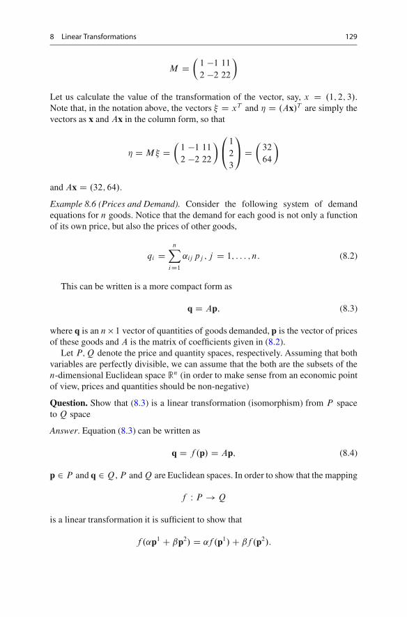
8 Linear Transformations 129
M D�
1 �1 11
2 �2 22
�
Let us calculate the value of the transformation of the vector, say, x D .1; 2; 3/.Note that, in the notation above, the vectors � D xT and � D .Ax/T are simply thevectors as x and Ax in the column form, so that
� DM � D�
1 �1 11
2 �2 22
�0
@1
2
3
1
A D�
32
64
�
and Ax D .32; 64/.
Example 8.6 (Prices and Demand). Consider the following system of demandequations for n goods. Notice that the demand for each good is not only a functionof its own price, but also the prices of other goods,
qi DnX
iD1
˛ij pj ; j D 1; : : : ; n: (8.2)
This can be written is a more compact form as
q D Ap; (8.3)
where q is an n� 1 vector of quantities of goods demanded, p is the vector of pricesof these goods and A is the matrix of coefficients given in (8.2).
Let P; Q denote the price and quantity spaces, respectively. Assuming that bothvariables are perfectly divisible, we can assume that the both are the subsets of then-dimensional Euclidean space Rn (in order to make sense from an economic pointof view, prices and quantities should be non-negative)
Question. Show that (8.3) is a linear transformation (isomorphism) from P spaceto Q space
Answer. Equation (8.3) can be written as
q D f .p/ D Ap; (8.4)
p 2 P and q 2 Q, P and Q are Euclidean spaces. In order to show that the mapping
f W P ! Q
is a linear transformation it is sufficient to show that
f .˛p1 C ˇp2/ D f .p1/C f .p2/:

130 8 Linear Transformations
From (8.4), by using matrix addition and multiplication of a matrix by a scalar, onecan easily obtain that
A.˛p1 C ˇp2/ D ˛A.p1/C ˇA.p2/:
Therefore, (8.4) is a linear transformation.
8.1 Addition and Multiplication of Linear Operators
Definition 8.5. Let R; S; T be 3 linear spaces and let A W R! S; B W S ! T andC W R! T be 3 linear transformations. The transformation C is the product of thetransformations A and B if for all x 2 R
C x D A.Bx/:
The product transformation C in the above definition is also linear, since
C.�1x1 C �2x2/ D AŒB.�1x1 C �2x2/�
D A.B�1x1 C B�2x2/ D �1ABx1 C �2ABx2
D �1C x1 C �2C x2
for all x1; x2 2 R and �1; �2 2 R.For example, one can multiply any linear operators acting in the same linear
space R. If I is the identity operator and A is an arbitrary operator in a linear spaceR, then
AI D IA D A:
Of a special interest, the powers of an operator A are defined as
A2 D AA; A3 D AA2; : : : ; An D AAn�1; : : : :
with A0 D I .
Example 8.7. Let us denote the operator of rotation of the plane R2 by an angle ˛
by A˛ . It follows that the product of two such operators A˛ and Aˇ is the rotationby the composite angle ˛ C ˇ
A˛Aˇ D A˛Cˇ:
Moreover, for every positive integer n the n-fold rotation by ˛ is the rotation by n˛,that is,
An˛ D An˛:
8.1 Addition and Multiplication of Linear Operators 131
Let A and B be two linear transformations as above while bA D kaikk andbB D kbikk be the corresponding transformation matrices with respect to the basise1; : : : ; en of R. Then, let us find the transformation matrix bC of the operatorC D AB . By definition
C ek DnX
iD1
cikei
and
ABek D A.
nX
j D1
bjkej / DnX
j D1
bjkAej DnX
iD1
nX
j D1
bjkaij ei :
Comparing the coefficients we obtain that C D AB if and only if
cik DnX
j D1
aij bjk
for all i; k D 1; : : : ; n, that is, the matrix of a product of transformations is a productof the matrices of the multipliers, bC D bAbB .
Example 8.8. Let A W R2 ! R2 and B W R3 ! R2 be two transformations withmatrices (denoted by the same letters)
A D�
0 1
1 1
�and B D
�0 1 10
0 2 20
�
For example, for x D .1; 2; 3/ we have (in the column vector form)
Bx D�
0 1 10
0 2 20
�0
@1
2
3
1
A D�
32
64
�and A.Bx/ D
�0 1
1 1
��32
64
�D�
64
96
�:
By the other hand, the matrix of the product transformation C D AB is
C D AB D�
0 1
1 1
��0 1 10
0 2 20
�D�
0 2 20
0 3 30
�;
so that
A.Bx/ D C x D�
0 2 20
0 3 30
�0
@1
2
3
1
A D�
64
96
�;
as before.
132 8 Linear Transformations
The addition of any two linear transformations A and B from R to S is also alinear transformation acting in the same vector spaces, denoted by C , such that forall x 2 R, C D .AC B/x � AxC Bx.
Let A and B be two linear transformations from R to S with A D kaikk andB D kbikk being the associated transformation matrices with respect to some basese1; : : : ; en of R and f1; : : : ; fm of S . Then, let us find the transformation matrix C ofthe operator C D AC B . We know that
Aek DPniD1 aikei
Bek DPn
iD1 bikei
C ek DPn
iD1 cikei :
On the other hand,
.ACB/ek DnX
iD1
.aik C bik/ei :
Hence C D AC B if and only if
cik D aik C bik
for all i; k D 1; : : : ; n, that is, the matrix of a sum of transformations is again a sumof their matrices.
Example 8.9. If A and B are two linear operators of R2 with matrices A D�
0 1
2 3
�
and B D�
10 20
30 40
�with respect to the canonical basis, then the sum C D ACB is
the operator with matrix C D�
10 21
32 43
�.
Remark 8.1. Since there is a one-to-one correspondence between the transfor-mations and transformation matrices, the properties of matrix multiplication andaddition (such as commutativity of addition, associativity of addition and multipli-cation, distributive law, etc.) are pertained by the linear operators as well.
8.2 Inverse Transformation, Image and Kernelunder a Transformation
The next definition is a particular case of Definition 8.2.
Definition 8.6. An operator B in a linear space R is said to be the inverse of anoperator A in R if
AB D BA D I;
where I is the identity operator.
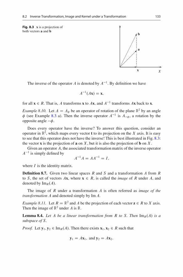
8.2 Inverse Transformation, Image and Kernel under a Transformation 133
Fig. 8.3 x is a projection ofboth vectors a and b
�
�
���������
��
���
�
b
a
x X
The inverse of the operator A is denoted by A�1. By definition we have
A�1.Ax/ D x;
for all x 2 R. That is, A transforms x to Ax; and A�1 transforms Ax back to x.
Example 8.10. Let A D A� be an operator of rotation of the plane R2 by an angle� (see Example 8.3 a). Then the inverse operator A�1 is A�� , a rotation by theopposite angle ��.
Does every operator have the inverse? To answer this question, consider anoperator in R2, which maps every vector t to its projection on the X axis. It is easyto see that this operator does not have the inverse! This is best illustrated in Fig. 8.3:the vector x is the projection of a on X , but it is also the projection of b on X .
Given an operator A, the associated transformation matrix of the inverse operatorA�1 is simply defined by
A�1A D AA�1 D I;
where I is the identity matrix.
Definition 8.7. Given two linear spaces R and S and a transformation A from R
to S , the set of vectors Ax, where x 2 R, is called the image of R under A, anddenoted by ImR.A/.
The image of R under a transformation A is often referred as image of thetransformation A and denoted simply by Im A.
Example 8.11. Let R D R2 and A be the projection of each vector z 2 R to X axis.Then the image of R2 under A is R.
Lemma 8.4. Let A be a linear transformation from R to S . Then ImR.A/ is asubspace of S .
Proof. Let y1; y2 2 ImR.A/. Then there exists x1; x2 2 R such that
y1 D Ax1; and y2 D Ax2:
134 8 Linear Transformations
Take any �1; �2 2 R. We have
�1y1 C �2y2 D �1Ax1 C �2Ax2
D A.�1x1 C �2x2/ 2 ImR.A/
for �1x1 C �2x2 2 R. �
Lemma 8.5. Let R be a linear space and A be a linear operator in R. If A has aninverse, then ImR.A/ D R.
Proof. Exercise. �
Definition 8.8. Given two spaces R and S and a transformation A from R to S , theset of vectors x, satisfying Ax D 0, is called the kernel of A in R, and is denoted byKerR.A/.
Lemma 8.6. Let R be a linear space and A be a linear transformation in R. ThenKerR.A/ is a subspace of R.
Proof. Exercise. �Theorem 8.7. Let R and S be two linear spaces and let A be a linear transfor-mation from R to S . Then the sum of the dimensions of the kernel and image of R
under A is equal to the dimension of R, that is
dim.ImR.A//C dim.KerR.A// D dim R
Proof. Let dim R D n and dim.KerR.A// D k � n. Select for KerR.A/, a basise1; : : : ; ek and complete it to a basis for R by the vectors ekC1; : : : ; en.
Consider the vectors AekC1; : : : ; Aen. The set of all linear combinations of thesevectors coincides with ImR.A/.
Now, take any y 2 ImR.A/. By definition, there exists x 2 R such that y D Ax.Since e1; : : : ; en is a basis for R, we have
x D �1e1 C � � � C �nen
for some �i ’s. Notice that Ae1 D Ae2 D � � � D Aek D 0 since e1; : : : ; ek is a basisfor KerR.A/. Hence, we have
y D Ax D �kC1AekC1 C � � � C �nAen:
Now let us show that n � k vectors given by AekC1; : : : ; Aen are linearly indepen-dent. Suppose on the contrary that there exist ˛1; : : : ; ˛n�k , not all being equal tozero such that
˛1AekC1 C � � � C ˛n�kAen D 0:
8.3 Linear Transformation Matrices with Respect to Different Bases 135
Consider now the vector x D ˛1ekC1 C � � � C ˛n�ken. We have
Ax D A.˛1ekC1 C � � � C ˛n�ken/ D ˛1AekC1 C � � � C ˛n�kAen D 0
implying x 2 KerR.A/. Thus we have obtained a contradiction, since x as an elementof the kernel can be represented through e1; : : : ; ek as well as the basis ekC1; : : : ; en
for the image, which is impossible as the vector x must have a unique representationwith respect to the basis e1; : : : ; en.
Hence, n� k vectors AekC1C � � � CAen are linearly independent, and thereforeany vector in ImR.A/ can be represented as a linear combination of n � k vectors,i.e. dim.ImR.A// D n � k. �
Example 8.12. Let A be an operator in R D R3 with the matrix (in the canonicalbasis)
A D2
40 1 1
1 0 1
0 1 1
3
5
The vector space ImR.A/ by the vectors Ae1; Ae2 and Ae3, that is, by the columnsof the above matrix A. The maximal number of linearly independent vectors amongthese three is 2 (because the third column is the sum of the first and second columns),hence dim ImR.A/ D 2. The kernel KerR.A/ consists of all vectors x which satisfythe equation Ax D 0, that is,
2
40 1 1
1 0 1
0 1 1
3
5 xT D2
40
0
0
3
5
The solutions of this equation are x D �.1; 1;�1/, so that KerR.A/ is a one-dimensional subspace spanned by the vector .1; 1;�1/.
8.3 Linear Transformation Matrices with Respectto Different Bases
Let R be an n-dimensional linear space with two bases e1; : : : ; en and f1; : : : ; fn. LetA be a linear operator in R, and C denote a matrix of transformation from e1; : : : ; en
to f1; : : : ; fn, i.e.,f1 D c11e1 C c21e2 C � � � C cn1en;
f2 D c12e1 C c22e2 C � � � C cn2en;
: : :
: : :
: : :
fn D c1ne1 C c2ne2 C � � � C cnnen:
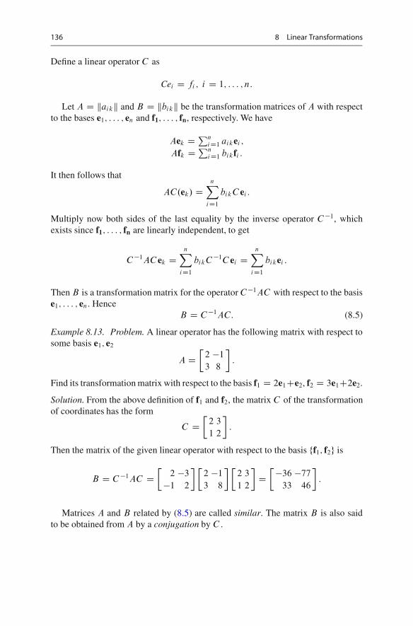
136 8 Linear Transformations
Define a linear operator C as
Cei D fi ; i D 1; : : : ; n:
Let A D kaikk and B D kbikk be the transformation matrices of A with respectto the bases e1; : : : ; en and f1; : : : ; fn, respectively. We have
Aek DPniD1 aikei ;
Afk DPn
iD1 bikfi :
It then follows that
AC.ek/ DnX
iD1
bikC ei :
Multiply now both sides of the last equality by the inverse operator C �1, whichexists since f1; : : : ; fn are linearly independent, to get
C �1AC ek DnX
iD1
bikC �1C ei DnX
iD1
bikei :
Then B is a transformation matrix for the operator C �1AC with respect to the basise1; : : : ; en. Hence
B D C �1AC: (8.5)
Example 8.13. Problem. A linear operator has the following matrix with respect tosome basis e1; e2
A D�
2 �1
3 8
�:
Find its transformation matrix with respect to the basis f1 D 2e1Ce2, f2 D 3e1C2e2.
Solution. From the above definition of f1 and f2, the matrix C of the transformationof coordinates has the form
C D�
2 3
1 2
�:
Then the matrix of the given linear operator with respect to the basis ff1; f2g is
B D C �1AC D�
2 �3
�1 2
� �2 �1
3 8
� �2 3
1 2
�D��36 �77
33 46
�:
Matrices A and B related by (8.5) are called similar. The matrix B is also saidto be obtained from A by a conjugation by C .
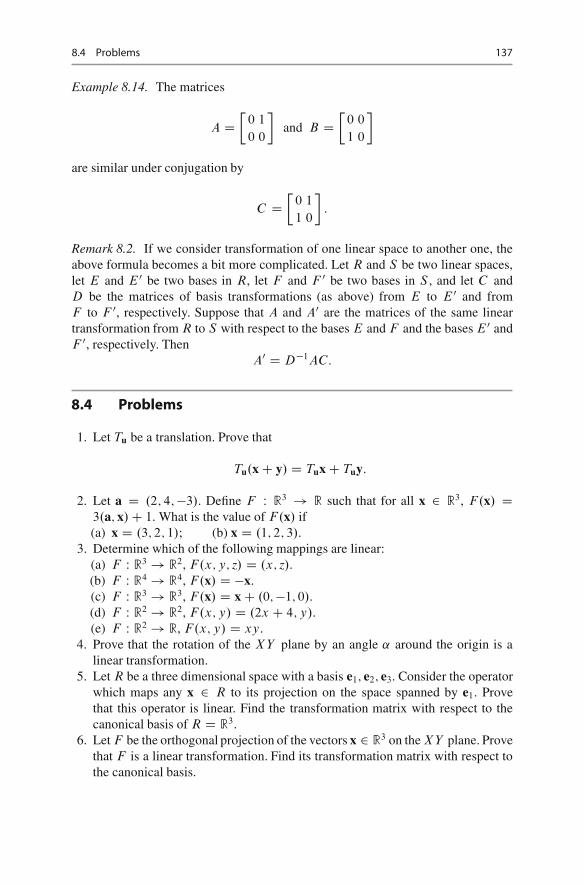
8.4 Problems 137
Example 8.14. The matrices
A D�
0 1
0 0
�and B D
�0 0
1 0
�
are similar under conjugation by
C D�
0 1
1 0
�:
Remark 8.2. If we consider transformation of one linear space to another one, theabove formula becomes a bit more complicated. Let R and S be two linear spaces,let E and E 0 be two bases in R, let F and F 0 be two bases in S , and let C andD be the matrices of basis transformations (as above) from E to E 0 and fromF to F 0, respectively. Suppose that A and A0 are the matrices of the same lineartransformation from R to S with respect to the bases E and F and the bases E 0 andF 0, respectively. Then
A0 D D�1AC:
8.4 Problems
1. Let Tu be a translation. Prove that
Tu.xC y/ D TuxC Tuy:
2. Let a D .2; 4;�3/. Define F W R3 ! R such that for all x 2 R3, F.x/ D3.a; x/C 1. What is the value of F.x/ if(a) x D .3; 2; 1/; (b) x D .1; 2; 3/.
3. Determine which of the following mappings are linear:(a) F W R3 ! R2, F.x; y; z/ D .x; z/.(b) F W R4 ! R4, F.x/ D �x.(c) F W R3 ! R3, F.x/ D xC .0;�1; 0/.(d) F W R2 ! R2, F.x; y/ D .2x C 4; y/.(e) F W R2 ! R, F.x; y/ D xy.
4. Prove that the rotation of the XY plane by an angle ˛ around the origin is alinear transformation.
5. Let R be a three dimensional space with a basis e1; e2; e3. Consider the operatorwhich maps any x 2 R to its projection on the space spanned by e1. Provethat this operator is linear. Find the transformation matrix with respect to thecanonical basis of R D R3.
6. Let F be the orthogonal projection of the vectors x 2 R3 on the XY plane. Provethat F is a linear transformation. Find its transformation matrix with respect tothe canonical basis.
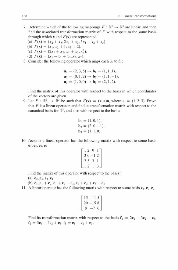
138 8 Linear Transformations
7. Determine which of the following mappings F W R3 ! R3 are linear, and thenfind the associated transformation matrix of F with respect to the same basisthrough which x and F.x/ are represented.(a) F.x/ D .x2 C x3; 2x1 C x3; 3x1 � x2 C x3/.(b) F.x/ D .x1; x2 C 1; x3 C 2/.(c) F.x/ D .2x1 C x2; x1 C x3; x2
3/.(d) F.x/ D .x1 � x2 C x3; x3; x2/.
8. Consider the following operator which maps each ai to bi :
a1 D .2; 3; 5/! b1 D .1; 1; 1/;
a2 D .0; 1; 2/! b2 D .1; 1;�1/;
a3 D .1; 0; 0/! b3 D .2; 1; 2/:
Find the matrix of this operator with respect to the basis in which coordinatesof the vectors are given.
9. Let F W R3 ! R3 be such that F.x/ D .x; a/a, where a D .1; 2; 3/. Provethat F is a linear operator, and find its transformation matrix with respect to thecanonical basis for R3, and also with respect to the basis:
b1 D .1; 0; 1/;
b2 D .2; 0;�1/;
b3 D .1; 1; 0/:
10. Assume a linear operator has the following matrix with respect to some basise1; e2; e3; e4 2
664
1 2 0 1
3 0 �1 2
2 5 3 1
1 2 1 3
3
775
Find the matrix of this operator with respect to the bases:(a) e2; e3; e4; e1
(b) e1; e1 C e2; e1 C e2 C e3; e1 C e2 C e3 C e4
11. A linear operator has the following matrix with respect to some basis e1; e2; e3
2
415 �11 5
20 �15 8
8 �7 6
3
5
Find its transformation matrix with respect to the basis f1 D 2e1 C 3e2 C e3,f2 D 3e1 C 4e2 C e3, f3 D e1 C e2 C e3.
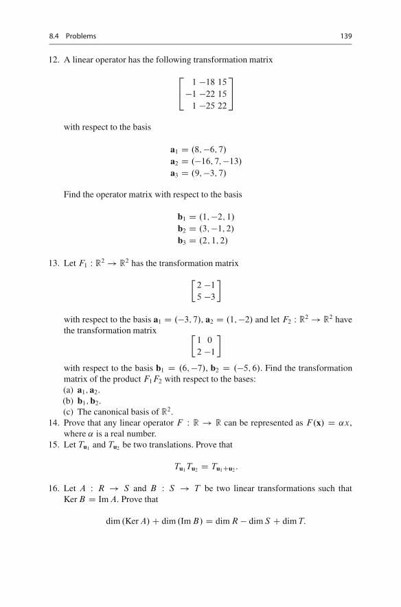
8.4 Problems 139
12. A linear operator has the following transformation matrix
2
41 �18 15
�1 �22 15
1 �25 22
3
5
with respect to the basis
a1 D .8;�6; 7/
a2 D .�16; 7;�13/
a3 D .9;�3; 7/
Find the operator matrix with respect to the basis
b1 D .1;�2; 1/
b2 D .3;�1; 2/
b3 D .2; 1; 2/
13. Let F1 W R2 ! R2 has the transformation matrix
�2 �1
5 �3
�
with respect to the basis a1 D .�3; 7/, a2 D .1;�2/ and let F2 W R2 ! R2 havethe transformation matrix �
1 0
2 �1
�
with respect to the basis b1 D .6;�7/, b2 D .�5; 6/. Find the transformationmatrix of the product F1F2 with respect to the bases:(a) a1; a2.(b) b1; b2.(c) The canonical basis of R2.
14. Prove that any linear operator F W R ! R can be represented as F.x/ D ˛x,where ˛ is a real number.
15. Let Tu1and Tu2
be two translations. Prove that
Tu1Tu2 D Tu1Cu2 :
16. Let A W R ! S and B W S ! T be two linear transformations such thatKer B D Im A. Prove that
dim .Ker A/C dim .Im B/ D dim R � dim S C dim T:

140 8 Linear Transformations
17. (a) Show that if the matrices A and B are conjugated, then the matrices B andA (the order is opposite to the given one) are conjugated as well.
(b) Show that if the matrix A is conjugated to B and B is conjugated to someC , then A is conjugated to C .
18. Let A and B be two conjugated matrices of order n. Prove that:(a) det A D det B .(b) rank A D rank B .(c) Tr A D Tr B .

9Eigenvectors and Eigenvalues
Let L be a linear space, L1 be a linear subspace of L and A be a linear operator in L.In general, for any vector x 2 L1, Ax may not belong to L1. The following examplemakes this claim clear. Let L D R2 and L1 D fx D .�1; �2/ 2 R2 j �1 D �2g, i.e.,L1 contains all vectors on the bisectrice of the Euclidean plane. Let A be a linearoperator in L such that for all x 2 L1, Ax D .�1; 2�2/. So, for all nonzero x 2 L1
we have Ax … L1 (Fig. 9.1).
Definition 9.1. Let A be a linear operator in a linear space L. Then the linearsubspace L1 of L is said to be invariant with respect to A if for all x 2 L1, Ax 2 L1.
Example 9.1. (a) Trivial invariant subspaces of any linear space L are f0g and Litself.
(b) Let L D R2. Given any x D �1e1 C �2e2 2 R2, where e1 D .1; 0/ and e2 D.0; 1/, we define
Ax D �1�1e1 C �2�2e2;
where �1; �2 2 R. Then, the axes of the Cartesian plane are invariant subspacesunder this operator.
(c) LetL be the set of all polynomials of degree at most n�1. Let A W P.t/! P 0.t/map each polynomial to its derivative. Then the set of all polynomials of degreeat most k, where 0 � k � n � 1 is an invariant subspace of L.
(d) Let L be any linear space and A be any linear operator in L. Consider KerL.A/
and ImL.A/. Both of these subspaces are invariant with respect to A.Let L1 be a one-dimensional subspace of the linear space L such that L1 D f˛y j
˛ 2 Rg for some nonzero y 2 L. Now L1 is invariant with respect to A if and onlyif for any x 2 L1 we have Ax 2 L1, i.e., Ax D �x for some � 2 R.
Definition 9.2. The non-zero vector x 2 L satisfying
Ax D �x
F. Aleskerov et al., Linear Algebra for Economists, Springer Texts in Businessand Economics, DOI 10.1007/978-3-642-20570-5 9,© Springer-Verlag Berlin Heidelberg 2011
141

142 9 Eigenvectors and Eigenvalues
Fig. 9.1 Ax … L1 for allnonzero x 2 L1
�
�
���������
��
���
���
��
��
�
Ax
x
�1
�2
2�2
0
L1
for some � 2 R, is called the eigenvector, while the corresponding � is called theeigenvalue, of the linear operator A.
Eigenvectors are also called characteristic vectors, and eigenvalues are alsocalled characteristic values of A.
Example 9.2. Let A D�
1 2
0 3
�be a linear operator. Let us find its eigenvectors x.
The equation Ax D �x gives
�1 2
0 3
� �x1
x2
�D �
�x1
x2
�;
or �.1 � �/x1 C 2x2 D 0;
.3 � �/x2 D 0:
It follows that there are two eigenvalues: � D 3 and � D 1. The eigenvectors arex D c.1; 1/ (for � D 3) and x D c.1; 0/ (for � D 1), where c is an arbitrary nonzeroreal number.
Example 9.3. (a) Let L be the set of all differentiable functions, and L1 be the setof all infinitely many times differentiable functions. Then the function
f .t/ D e�t
with � 2 R, is an eigenvector of the linear operator A D d=dt sincedf .t/=dt D �f .t/.
(b) Let 2
664
a1 0:
::
0 an
3
775
be the transformation matrix of a linear operator A. Then for all i D 1; : : : ; n
the unit vector
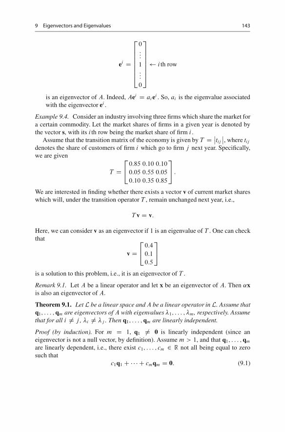
9 Eigenvectors and Eigenvalues 143
ei D
2
6666664
0:::
1:::
0
3
7777775
i th row
is an eigenvector of A. Indeed, Aei D ai ei . So, ai is the eigenvalue associatedwith the eigenvector ei .
Example 9.4. Consider an industry involving three firms which share the market fora certain commodity. Let the market shares of firms in a given year is denoted bythe vector s, with its i th row being the market share of firm i .
Assume that the transition matrix of the economy is given by T D ˇˇtijˇˇ, where tij
denotes the share of customers of firm i which go to firm j next year. Specifically,we are given
T D2
40:85 0:10 0:10
0:05 0:55 0:05
0:10 0:35 0:85
3
5 :
We are interested in finding whether there exists a vector v of current market shareswhich will, under the transition operator T , remain unchanged next year, i.e.,
T v D v:
Here, we can consider v as an eigenvector if 1 is an eigenvalue of T . One can checkthat
v D2
40:4
0:1
0:5
3
5
is a solution to this problem, i.e., it is an eigenvector of T .
Remark 9.1. Let A be a linear operator and let x be an eigenvector of A. Then ˛xis also an eigenvector of A.
Theorem 9.1. Let L be a linear space and A be a linear operator in L. Assume thatq1; : : : ; qm are eigenvectors of A with eigenvalues �1; : : : ; �m, respectively. Assumethat for all i ¤ j , �i ¤ �j . Then q1; : : : ; qm are linearly independent.
Proof (by induction). For m D 1, q1 ¤ 0 is linearly independent (since aneigenvector is not a null vector, by definition). Assume m > 1, and that q1; : : : ; qm
are linearly dependent, i.e., there exist c1; : : : ; cm 2 R not all being equal to zerosuch that
c1q1 C � � � C cmqm D 0: (9.1)
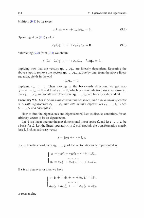
144 9 Eigenvectors and Eigenvalues
Multiply (9.1) by �1 to get
c1�1q1 C � � � C cm�1qm D 0: (9.2)
Operating A on (9.1) yields
c1�1q1 C � � � C cm�mqm D 0: (9.3)
Subtracting (9.2) from (9.3) we obtain
c2.�2 � �1/q2 C � � � C cm.�m � �1/qm D 0;
implying now that the vectors q2; : : : ; qm are linearly dependent. Repeating theabove steps to remove the vectors q2; : : : ; qm�1, one by one, from the above linearequation, yields in the end
cmqm D 0;
implying cm D 0. Then moving in the backwards direction, we get alsoc2 D � � � D cm D 0, and finally c1 D 0, which is a contradiction, since we assumedthat c1; : : : ; cm are not all zero. Therefore, q1; : : : ; qm are linearly independent.
Corollary 9.2. Let L be an n-dimensional linear space, and A be a linear operatorin L with eigenvectors e1; : : : ; en and with distinct eigenvalues �1; : : : ; �n. Thene1; : : : ; en is a basis for L.
How to find the eigenvalues and eigenvectors? Let us discuss conditions for anarbitrary vector to be an eigenvector.
Let A is a linear operator in an n-dimensional linear space L, and let e1; : : : ; en bea basis for L. Let the linear operator A in L corresponds the transformation matrixkaikk. Pick an arbitrary vector
x D �1e1 C � � � C �nen
in L. Then the coordinates �1; : : : ; �n of the vector Ax can be represented as
8<
:
�1 D a11�1 C a12�2 C � � � C a1n�n;
: : : : : : ::
�n D an1�1 C an2�2 C � � � C ann�n:
If x is an eigenvector then we have
8<
:
a11�1 C a12�2 C � � � C a1n�n D ��1;
: : : : : : ::
an1�1 C an2�2 C � � � C ann�n D ��n;
or rearranging
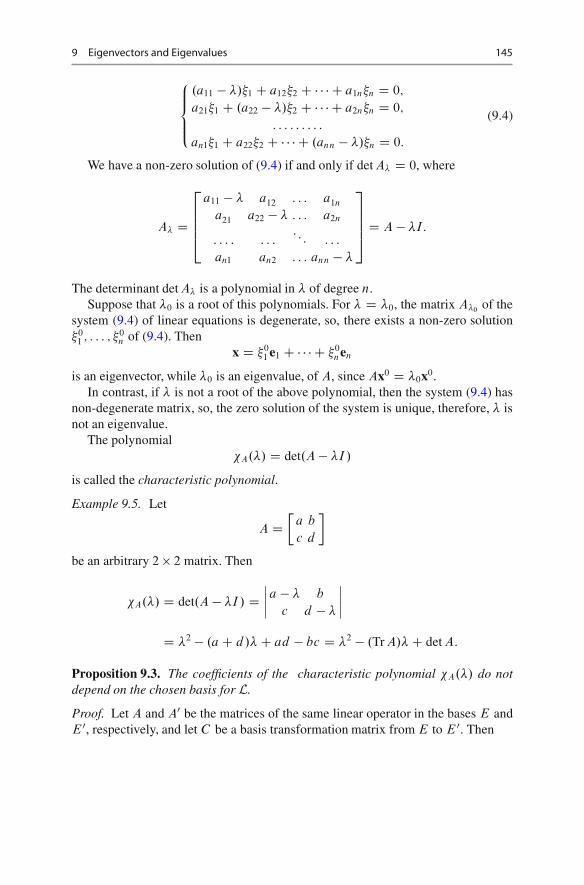
9 Eigenvectors and Eigenvalues 145
8ˆ<
ˆ:
.a11 � �/�1 C a12�2 C � � � C a1n�n D 0;
a21�1 C .a22 � �/�2 C � � � C a2n�n D 0;
: : : : : : : : :
an1�1 C a22�2 C � � � C .ann � �/�n D 0:
(9.4)
We have a non-zero solution of (9.4) if and only if det A� D 0, where
A� D
2
6664
a11 � � a12 : : : a1n
a21 a22 � � : : : a2n
: : : : : : :: : : : : :
an1 an2 : : : ann � �
3
7775D A � �I:
The determinant det A� is a polynomial in � of degree n.Suppose that �0 is a root of this polynomials. For � D �0, the matrix A�0
of thesystem (9.4) of linear equations is degenerate, so, there exists a non-zero solution�0
1 ; : : : ; �0n of (9.4). Then
x D �01 e1 C � � � C �0
nen
is an eigenvector, while �0 is an eigenvalue, of A, since Ax0 D �0x0.In contrast, if � is not a root of the above polynomial, then the system (9.4) has
non-degenerate matrix, so, the zero solution of the system is unique, therefore, � isnot an eigenvalue.
The polynomial�A.�/ D det.A� �I/
is called the characteristic polynomial.
Example 9.5. Let
A D�
a b
c d
�
be an arbitrary 2 � 2 matrix. Then
�A.�/ D det.A � �I/ Dˇˇˇˇa � � b
c d � �
ˇˇˇˇ
D �2 � .aC d/�C ad � bc D �2 � .Tr A/�C det A:
Proposition 9.3. The coefficients of the characteristic polynomial �A.�/ do notdepend on the chosen basis for L.
Proof. Let A and A0 be the matrices of the same linear operator in the bases E andE 0, respectively, and let C be a basis transformation matrix from E to E 0. Then

146 9 Eigenvectors and Eigenvalues
�0A.�/ D det.A0 � �I/ D det.C �1AC � �I/ D det.C �1AC � �C �1C /
D det�C �1.A� �I/C
� D det C �1 det.A� �I/ det C
D det.A� �I/ D �A.�/:
�Hence, it is called the characteristic polynomial of the linear operator A, but not
that of the transformation matrix A.Thus we obtain
Theorem 9.4. Let A be a linear operator in an n-dimensional linear space. Theneach eigenvalue of A is a root of the characteristic polynomial �A.�/, and each rootof this polynomial is an eigenvalue.
To describe the eigenvectors x corresponding to a given root �0, one should solvethe system (9.4) of linear equations, that is, the system
.A� �0I /x D 0:
Until now we have considered linear spaces over real numbers. In fact, ourresults remain valid if we consider linear spaces over complex numbers (we discusscomplex numbers in Appendix C). We formulate this as our next result.
Corollary 9.5. For every complex vector space L, any linear operator A in L hasat least one eigenvector.
Proof. The polynomial �A.�/ is always of positive degree. Such a polynomialis known to have at least one (complex) root �0 (the fundamental theorem ofalgebra, see Theorem C.1). Then it is a (complex) eigenvalue, and the correspondingeigenvector x (probably, with complex coefficients) may be obtained as a solutionof (9.4). �
Now let A be a linear operator in L and e1; : : : ; en be its linearly independenteigenvectors, i.e.
Aei D �i ei ; i D 1; : : : ; n: (9.5)
Let us choose e1; : : : ; en as a basis for L. Then the above equalities imply that thetransformation matrix of A with respect to this basis is
2
6664
�1 0 : : : 0
0 �2 : : : 0:::
:::: : :
:::
0 0 : : : �n
3
7775
;
which is called the diagonal matrix. Hence, we prove the following
Theorem 9.6. If a linear operator A 2 L has n linearly independent eigenvectors,then choosing them as a basis for L, we can represent the transformation matrix of
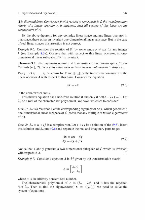
9 Eigenvectors and Eigenvalues 147
A in diagonal form. Conversely, if with respect to some basis in L the transformationmatrix of a linear operator A is diagonal, then all vectors of this basis are theeigenvectors of A.
By the above theorem, for any complex linear space and any linear operator inthat space, there exists an invariant one-dimensional linear subspace. But in the caseof real linear spaces this assertion is not correct.
Example 9.6. Consider the rotation of R2 by some angle � ¤ k� for any integerk (see Example 8.3a). Observe that with respect to this linear operator, no one-dimensional linear subspace of R2 is invariant.
Theorem 9.7. For any linear operator A in an n-dimensional linear space L overthe reals (n � 2), there exist either one- or two-dimensional invariant subspaces.
Proof. Let e1; : : : ; en be a basis for L and kaikk be the transformation matrix of thelinear operator A with respect to this basis. Consider the equation
Ax D �x (9.6)
in the unknowns x and �.This matrix equation has a non-zero solution if and only if det.A� �I/ D 0. Let
�0 be a root of the characteristic polynomial. We have two cases to consider:
Case 1: �0 is a real root. Let the corresponding eigenvector be x, which generates aone-dimensional linear subspace of L (recall that any multiple of x is an eigenvectorof A).
Case 2: �0 D ˛C iˇ is a complex root. Let xC iy be a solution of the (9.6). Insertthis solution and �0 into (9.6) and separate the real and imaginary parts to get
Ax D ˛x � ˇyAy D ˛yC ˇx:
(9.7)
Notice that x and y generate a two-dimensional subspace of L which is invariantwith respect to A. �Example 9.7. Consider a operator A in R2 given by the transformation matrix
A D�
�0 0
� �0
�
where � is an arbitrary nonzero real number.The characteristic polynomial of A is .�0 � �/2, and it has the repeated
root �0. Then to find the eigenvector(s) x D .�1; �2/, we need to solve thesystem of equations

148 9 Eigenvectors and Eigenvalues
�0�1 C 0�2 D 0
��1 C 0�2 D 0:
The above system adopts the unique non-zero solution �1 D 0, �2 D 1 (up to aconstant multiple). Then the corresponding invariant subspace of R2 is of dimensionone, which is less than the number of roots of the characteristic polynomial.
9.1 Macroeconomic Example: Growth and Consumption
9.1.1 The Model
Consider an n-sector economy that produces n goods denoted by the vectorx. All goods are both used as inputs in production and consumed by workers.The commodity input requirements of production is given by n � n input/outputcoefficients matrix A and labor requirements by labor/output coefficients rowvector a. (Notice that all the elements of A and a are non-negative). It is assumedthat the consumption basket of workers is given by the column vector c. (This canbe interpreted as a wage basket that reflects social minimum wage, determined bysocial and historical conditions of the society in question.)
This system of production and its use can be summarized as follows:OutputD input requirements of production+ consumption (of workers), or
x D AxC cax:
This economy uses all its output for current production and consumption,therefore it is incapable of growing. Now let us introduce growth into this picture.For the sake of simplicity suppose that policy makers aim at growing all sectors atthe same rate, i.e. on a ‘balanced growth path’. Therefore, the extra amount of goodsnecessary for achieving this growth performance is given by
s D gŒAxC cax; (9.8)
where g is the balanced growth rate (a scalar) of the economy. When (9.8) is takeninto account, the production system becomes
x D AxC caxC gŒAxC cax; (9.9)
where the first term in the right hand corresponds to the input requirements forcurrent consumption and the second term stands for the input requirements ofgrowth. Let us define
B D AC ca

9.1 Macroeconomic Example: Growth and Consumption 149
As the ‘augmented input matrix’, i.e., that takes into account the consumption needsof the labor, and treats the latter as an input of production. Therefore, (9.9) can berewritten as
x D .1C g/Bx: (9.10)
Question 1. Suppose that the policy makers want to know the maximum feasiblerate of growth of such economy, given the technology .A; a/ and exogenously givenconsumption basket of the workers, c.
Answer. Notice that (9.10) can be rewritten as
Œ�I � Bx D 0; (9.11)
where � D .1C g/� 1, I is the n� n identity matrix and 0 is the n� 1 zero vector.From (9.11) it is clear that the required answer can be obtained by the eigenvaluesand corresponding eigenvectors of the matrix B and picking the one that allowsmaximum rate of growth. Obviously in this context a production system is feasibleif at least it can sustain itself, i.e., g is a non-negative scalar and correspondingeigenvector is also non-negative.
9.1.2 Numerical Example
Suppose the technology of the economy is given by the following input/outputmatrix A, and labor/output vector a
A D2
40:120 0:170 0:120
0:140 0:110 0:140
0:110 0:130 0:110
3
5 ;
a D Œ0:36; 0:37; 0:40:
Let the consumption vector be
c D2
40:6
0:45
0:45
3
5 :
Using this information, the augmented input coefficients matrix can becalculated as
B D AC ca D2
40:336 0:392 0:360
0:253 0:277 0:320
0:272 0:297 0:290
3
5 :

150 9 Eigenvectors and Eigenvalues
The eigenvalues of the matrix B are
�1 D 0;9458; �2 D �0;0003; �3 D �0;0425:
Only the first eigenvalue is positive. Therefore, the others have no economicmeaning. The eigenvector that corresponds to �1 is .0:6574; 0:5455; 0:5197/. Thetechnically maximum feasible growth rate for this economy is
g D .1 � �/=� D 5; 7
Question 1. Can this economy afford a 10% increase in the consumption goodvector of workers?
(Hint: Change the consumption vector by increasing its each component by10%. Then calculate the eigenvalues of the augmented matrix and check if thecorresponding maximum feasible growth rate is non-negative or not.)
9.2 Self-Adjoint Operators
A linear operator A in a real Euclidean space E is called self-adjoint if for allx; y 2 E
.Ax; y/ D .x; Ay/: (9.12)
Example 9.8. Let us show that the operator A D��1 4
4 5
�is self-adjoint. Indeed,
for x D .x1; x2/ and y D .y1; y2/ we have Ax D .�x1 C 4x2; 4x1 C 5x2/ andAy D .�y1 C 4y2; 4y1 C 5y2/, so that
.Ax; y/ D �x1y1 C 4x2y1 C 4x1y2 C 5x2y2 D .x; Ay/:
Theorem 9.8. Any linear operator A in a real Euclidean space E is self-adjointif and only if for any orthogonal basis of E , the transformation matrix of A issymmetric.
Proof. Let e1; : : : ; en be an orthogonal basis for E . Pick any two vectors
x D �1e1 C � � � C �nen
y D �1e1 C � � � C �nen
in E . Let 1; : : : ; n be coordinates of the vector z D Ax, i.e.
i DnX
kD1
aik�k;
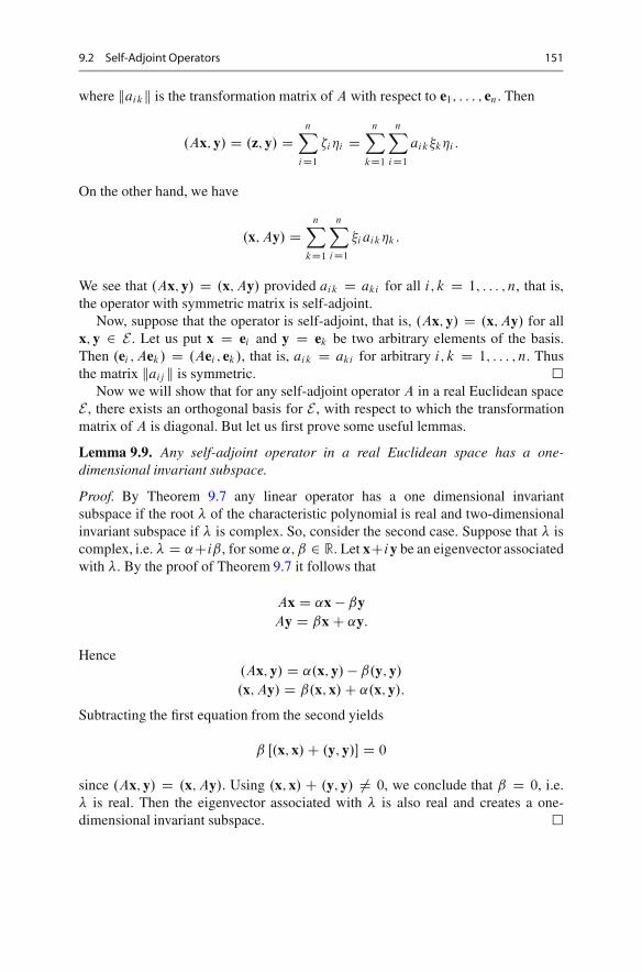
9.2 Self-Adjoint Operators 151
where kaikk is the transformation matrix of A with respect to e1; : : : ; en. Then
.Ax; y/ D .z; y/ DnX
iD1
i�i DnX
kD1
nX
iD1
aik�k�i :
On the other hand, we have
.x; Ay/ DnX
kD1
nX
iD1
�i aik�k:
We see that .Ax; y/ D .x; Ay/ provided aik D aki for all i; k D 1; : : : ; n, that is,the operator with symmetric matrix is self-adjoint.
Now, suppose that the operator is self-adjoint, that is, .Ax; y/ D .x; Ay/ for allx; y 2 E . Let us put x D ei and y D ek be two arbitrary elements of the basis.Then .ei ; Aek/ D .Aei ; ek/, that is, aik D aki for arbitrary i; k D 1; : : : ; n. Thusthe matrix kaij k is symmetric. �
Now we will show that for any self-adjoint operator A in a real Euclidean spaceE , there exists an orthogonal basis for E , with respect to which the transformationmatrix of A is diagonal. But let us first prove some useful lemmas.
Lemma 9.9. Any self-adjoint operator in a real Euclidean space has a one-dimensional invariant subspace.
Proof. By Theorem 9.7 any linear operator has a one dimensional invariantsubspace if the root � of the characteristic polynomial is real and two-dimensionalinvariant subspace if � is complex. So, consider the second case. Suppose that � iscomplex, i.e. � D ˛Ciˇ, for some ˛; ˇ 2 R. Let xCiy be an eigenvector associatedwith �. By the proof of Theorem 9.7 it follows that
Ax D ˛x � ˇyAy D ˇxC ˛y:
Hence.Ax; y/ D ˛.x; y/� ˇ.y; y/
.x; Ay/ D ˇ.x; x/C ˛.x; y/:
Subtracting the first equation from the second yields
ˇ Œ.x; x/C .y; y/ D 0
since .Ax; y/ D .x; Ay/. Using .x; x/ C .y; y/ ¤ 0, we conclude that ˇ D 0, i.e.� is real. Then the eigenvector associated with � is also real and creates a one-dimensional invariant subspace. �
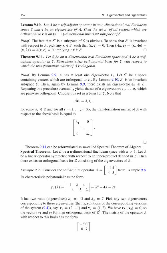
152 9 Eigenvectors and Eigenvalues
Lemma 9.10. Let A be a self-adjoint operator in an n-dimensional real Euclideanspace E and e be an eigenvector of A. Then the set E 0 of all vectors which areorthogonal to e is an .n � 1/-dimensional invariant subspace of E .
Proof. The fact that E 0 is a subspace of E is obvious. To show that E 0 is invariantwith respect to A, pick any x 2 E 0 such that .x; e/ D 0. Then .Ax; e/ D .x; Ae/ D.x; �e/ D �.x; e/ D 0, implying Ax 2 E 0. �
Theorem 9.11. Let E be an n-dimensional real Euclidean space and A be a self-adjoint operator in E . Then there exists orthonormal basis for E with respect towhich the transformation matrix of A is diagonal.
Proof. By Lemma 9.9, A has at least one eigenvector e1. Let E 0
be a spacecontaining vectors which are orthogonal to e1. By Lemma 9.10, E 0
is an invariantsubspace E . Then, again by Lemma 9.9, there exists an eigenvector e2 2 E 0
.Repeating this procedure eventually yields the set of n eigenvectors e1; : : : ; en whichare pairwise orthogonal. Choose this set as a basis for E . Note that
Aei D �i ei ;
for some �i 2 R and for all i D 1; : : : ; n. So, the transformation matrix of A withrespect to the above basis is equal to
2
64
�1 0: : :
0 �n
3
75 :
�Theorem 9.11 can be reformulated as so-called Spectral Theorem of Algebra.
Spectral Theorem. Let L be a n-dimensional Euclidean space with n > 1. Let A
be a linear operator symmetric with respect to an inner-product defined in L. Thenthere exists an orthogonal basis for L consisting of the eigenvectors of A.
Example 9.9. Consider the self-adjoint operator A D��1 4
4 5
�from Example 9.8.
Its characteristic polynomial has the form
�A.�/ Dˇˇˇˇ�1 � � 4
4 5 � �
ˇˇˇˇ D �2 � 4� � 21:
It has two roots (eigenvalues) �1 D �3 and �2 D 7. Pick any two eigenvectorscorresponding to these eigenvalues (that is, solutions of the corresponding versionsof the system (9.4)), say, v1 D .2;�1/ and v2 D .1; 2/. We have .v1; v2/ D 0, sothe vectors v1 and v2 form an orthogonal basis of R2. The matrix of the operator A
with respect to this basis has the form��3 0
0 7
�

9.3 Orthogonal Operators 153
9.3 Orthogonal Operators
Definition 9.3. A linear operator A in a real n-dimensional Euclidean space E iscalled orthogonal operator if for all x; y 2 E
.Ax; Ay/ D .x; y/: (9.13)
Example 9.10. The matrix A D�
1=2p
3=2
�p3=2 1=2
�is orthogonal.
Note that orthogonal operators preserves the inner-product. To see a specialimplication of this observation, insert x D y into (9.13) to obtain
jAxj2 D jxj2 :
Hence orthogonal operator preserves the length of a vector.Now pick any e1; : : : ; en orthogonal basis for E . Then we have
.Aei ; Aek/ D�
1; if i D k;
0; otherwise.(9.14)
Note that, on the other side, any operator A which satisfies (9.14) is orthogonal.Let kaikk be the transformation matrix of A with respect to this basis. The i th
column of this matrix contains the coordinates of Aei , hence (9.14) can be rewrittenas
nX
j D1
aj i ajk D�
1; if i D k;
0; otherwise.
ButPn
j D1 aj i ajk is the ik-th element of the product AT A, hence it is also true that
AT A D I:
Thus, we havedet.A/ D ˙1;
i.e., the determinant of the orthogonal transformation matrix is either C1 or �1.An orthogonal operator A is called non-singular if det.A/ D C1 and singular ifdet.A/ D �1.
(Do not confuse with singular matrix A for which det A D 0!)
Lemma 9.12. Let L be a linear space, A be an orthogonal linear operator in L,and L1 be a subspace of L invariant with respect to A. Then orthogonal complementL2 of L1 (the set of all vectors y 2 L orthogonal to each x 2 L1) is also an invariantsubspace.
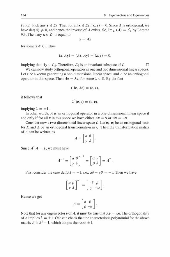
154 9 Eigenvectors and Eigenvalues
Proof. Pick any y 2 L2. Then for all x 2 L1, .x; y/ D 0. Since A is orthogonal, wehave det.A/ ¤ 0, and hence the inverse of A exists. So, ImL1 .A/ D L1 by Lemma9.3. Then any x 2 L1 is equal to
x D Az
for some z 2 L1. Thus
.x; Ay/ D .Az; Ay/ D .z; y/ D 0;
implying that Ay 2 L2. Therefore, L2 is an invariant subspace of L. �We can now study orthogonal operators in one and two dimensional linear spaces.
Let e be a vector generating a one-dimensional linear space, and A be an orthogonaloperator in this space. Then Ae D �e, for some � 2 R. By the fact
.Ae; Ae/ D .e; e/;
it follows that�2.e; e/ D .e; e/;
implying � D ˙1.In other words, A is an orthogonal operator in a one-dimensional linear space if
and only if for all x in this space we have either Ax D x or Ax D �x.Consider now a two-dimensional linear space L. Let e1; e2 be an orthogonal basis
for L and A be an orthogonal transformation in L. Then the transformation matrixof A can be written as
A D�
˛ ˇ
� ı
�:
Since AT A D I , we must have
A�1 D�
˛ ˇ
� ı
��1
D�
˛ �
ˇ ı
�D AT :
First consider the case det.A/ D �1, i.e., ˛ı � �ˇ D �1. Then we have
�˛ ˇ
� ı
��1
D��ı ˇ
� �˛
�:
Hence we get
A D�
˛ ˇ
ˇ �˛
�:
Note that for any eigenvector e of A, it must be true that Ae D �e. The orthogonalityof A implies � D ˙1. One can check that the characteristic polynomial for the abovematrix A is �2 � 1, which adopts the roots˙1.
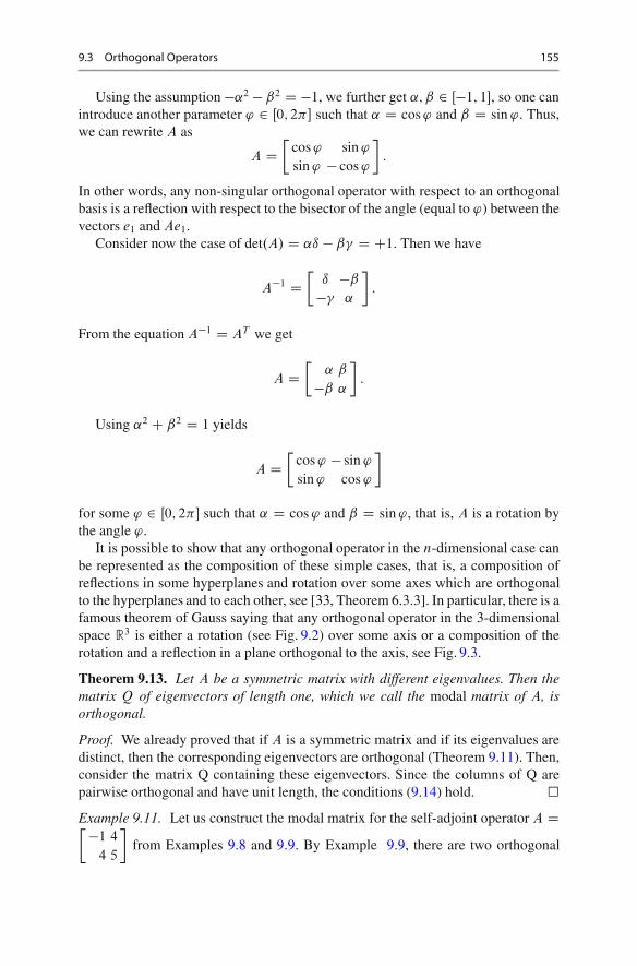
9.3 Orthogonal Operators 155
Using the assumption �˛2 � ˇ2 D �1, we further get ˛; ˇ 2 Œ�1; 1, so one canintroduce another parameter ' 2 Œ0; 2� such that ˛ D cos ' and ˇ D sin '. Thus,we can rewrite A as
A D�
cos ' sin '
sin ' � cos '
�:
In other words, any non-singular orthogonal operator with respect to an orthogonalbasis is a reflection with respect to the bisector of the angle (equal to ') between thevectors e1 and Ae1.
Consider now the case of det.A/ D ˛ı � ˇ� D C1. Then we have
A�1 D�
ı �ˇ
�� ˛
�:
From the equation A�1 D AT we get
A D�
˛ ˇ
�ˇ ˛
�:
Using ˛2 C ˇ2 D 1 yields
A D�
cos ' � sin '
sin ' cos '
�
for some ' 2 Œ0; 2� such that ˛ D cos ' and ˇ D sin ', that is, A is a rotation bythe angle '.
It is possible to show that any orthogonal operator in the n-dimensional case canbe represented as the composition of these simple cases, that is, a composition ofreflections in some hyperplanes and rotation over some axes which are orthogonalto the hyperplanes and to each other, see [33, Theorem 6.3.3]. In particular, there is afamous theorem of Gauss saying that any orthogonal operator in the 3-dimensionalspace R3 is either a rotation (see Fig. 9.2) over some axis or a composition of therotation and a reflection in a plane orthogonal to the axis, see Fig. 9.3.
Theorem 9.13. Let A be a symmetric matrix with different eigenvalues. Then thematrix Q of eigenvectors of length one, which we call the modal matrix of A, isorthogonal.
Proof. We already proved that if A is a symmetric matrix and if its eigenvalues aredistinct, then the corresponding eigenvectors are orthogonal (Theorem 9.11). Then,consider the matrix Q containing these eigenvectors. Since the columns of Q arepairwise orthogonal and have unit length, the conditions (9.14) hold. �
Example 9.11. Let us construct the modal matrix for the self-adjoint operator A D��1 4
4 5
�from Examples 9.8 and 9.9. By Example 9.9, there are two orthogonal
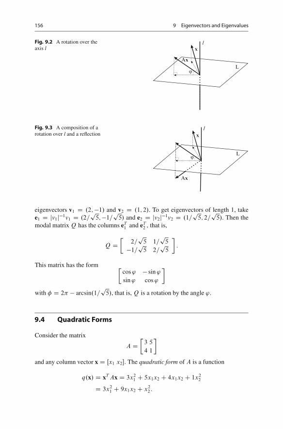
156 9 Eigenvectors and Eigenvalues
Fig. 9.2 A rotation over theaxis l
l
Lϕ
x
Ax
Fig. 9.3 A composition of arotation over l and a reflection
l
Lϕ
x
Ax
eigenvectors v1 D .2;�1/ and v2 D .1; 2/. To get eigenvectors of length 1, takee1 D jv1j�1v1 D .2=
p5;�1=
p5/ and e2 D jv2j�1v2 D .1=
p5; 2=p
5/. Then themodal matrix Q has the columns eT
1 and eT2 , that is,
Q D�
2=p
5 1=p
5
�1=p
5 2=p
5
�:
This matrix has the form �cos ' � sin '
sin ' cos '
�
with � D 2� � arcsin.1=p
5/, that is, Q is a rotation by the angle '.
9.4 Quadratic Forms
Consider the matrix
A D�
3 5
4 1
�
and any column vector x D Œx1 x2. The quadratic form of A is a function
q.x/ D xT Ax D 3x21 C 5x1x2 C 4x1x2 C 1x2
2
D 3x21 C 9x1x2 C x2
2:
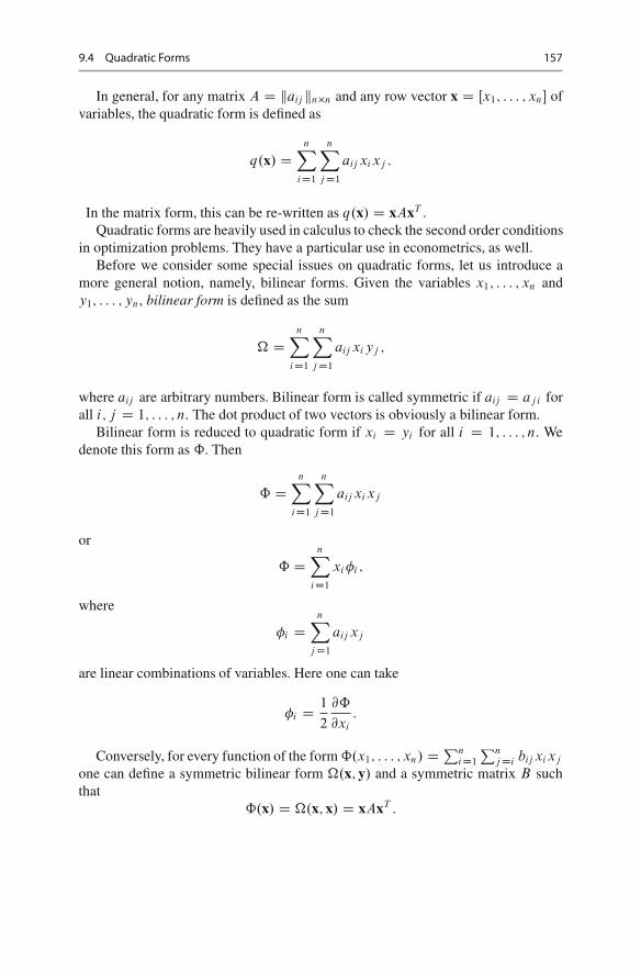
9.4 Quadratic Forms 157
In general, for any matrix A D kaij kn�n and any row vector x D Œx1; : : : ; xn ofvariables, the quadratic form is defined as
q.x/ DnX
iD1
nX
j D1
aij xixj :
In the matrix form, this can be re-written as q.x/ D xAxT .Quadratic forms are heavily used in calculus to check the second order conditions
in optimization problems. They have a particular use in econometrics, as well.Before we consider some special issues on quadratic forms, let us introduce a
more general notion, namely, bilinear forms. Given the variables x1; : : : ; xn andy1; : : : ; yn, bilinear form is defined as the sum
� DnX
iD1
nX
j D1
aij xi yj ;
where aij are arbitrary numbers. Bilinear form is called symmetric if aij D aj i forall i; j D 1; : : : ; n. The dot product of two vectors is obviously a bilinear form.
Bilinear form is reduced to quadratic form if xi D yi for all i D 1; : : : ; n. Wedenote this form as ˆ. Then
ˆ DnX
iD1
nX
j D1
aij xi xj
or
ˆ DnX
iD1
xi �i ;
where
�i DnX
j D1
aij xj
are linear combinations of variables. Here one can take
�i D 1
2
@ˆ
@xi
:
Conversely, for every function of the form ˆ.x1; : : : ; xn/ DPniD1
Pnj Di bij xi xj
one can define a symmetric bilinear form �.x; y/ and a symmetric matrix B suchthat
ˆ.x/ D �.x; x/ D xAxT :
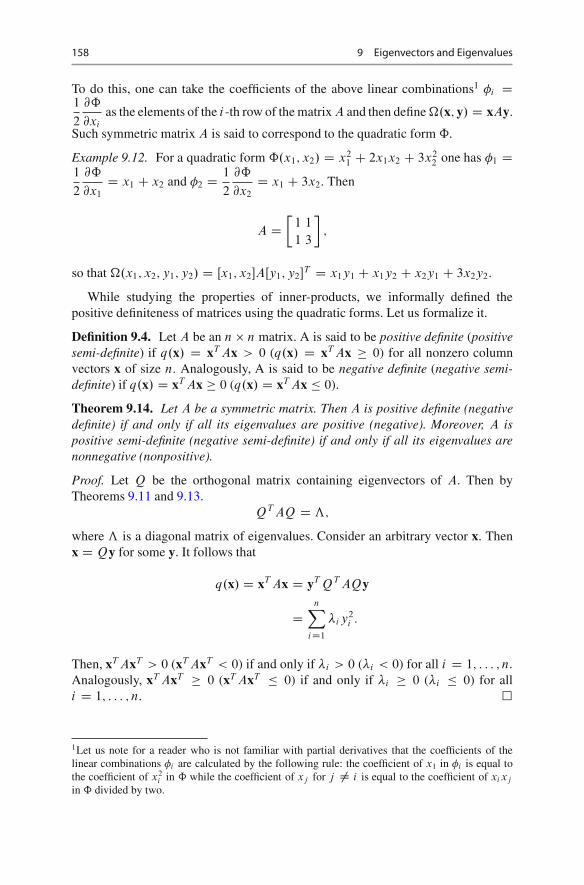
158 9 Eigenvectors and Eigenvalues
To do this, one can take the coefficients of the above linear combinations1 �i D1
2
@ˆ
@xi
as the elements of the i -th row of the matrix A and then define �.x; y/ D xAy.
Such symmetric matrix A is said to correspond to the quadratic form ˆ.
Example 9.12. For a quadratic form ˆ.x1; x2/ D x21 C 2x1x2 C 3x2
2 one has �1 D1
2
@ˆ
@x1
D x1 C x2 and �2 D 1
2
@ˆ
@x2
D x1 C 3x2. Then
A D�
1 1
1 3
�;
so that �.x1; x2; y1; y2/ D Œx1; x2AŒy1; y2T D x1y1 C x1y2 C x2y1 C 3x2y2.
While studying the properties of inner-products, we informally defined thepositive definiteness of matrices using the quadratic forms. Let us formalize it.
Definition 9.4. Let A be an n � n matrix. A is said to be positive definite (positivesemi-definite) if q.x/ D xT Ax > 0 (q.x/ D xT Ax � 0) for all nonzero columnvectors x of size n. Analogously, A is said to be negative definite (negative semi-definite) if q.x/ D xT Ax � 0 (q.x/ D xT Ax � 0).
Theorem 9.14. Let A be a symmetric matrix. Then A is positive definite (negativedefinite) if and only if all its eigenvalues are positive (negative). Moreover, A ispositive semi-definite (negative semi-definite) if and only if all its eigenvalues arenonnegative (nonpositive).
Proof. Let Q be the orthogonal matrix containing eigenvectors of A. Then byTheorems 9.11 and 9.13.
QT AQ D ƒ;
where ƒ is a diagonal matrix of eigenvalues. Consider an arbitrary vector x. Thenx D Qy for some y. It follows that
q.x/ D xT Ax D yT QT AQy
DnX
iD1
�iy2i :
Then, xT AxT > 0 (xT AxT < 0) if and only if �i > 0 (�i < 0) for all i D 1; : : : ; n.Analogously, xT AxT � 0 (xT AxT � 0) if and only if �i � 0 (�i � 0) for alli D 1; : : : ; n. �
1Let us note for a reader who is not familiar with partial derivatives that the coefficients of thelinear combinations �i are calculated by the following rule: the coefficient of x1 in �i is equal tothe coefficient of x2
i in ˆ while the coefficient of xj for j ¤ i is equal to the coefficient of xi xj
in ˆ divided by two.

9.4 Quadratic Forms 159
It is sometimes hard to apply the above theorem to check if a quadratic form ispositive (or negative) definite, because there is no simple general method to calculatethe eigenvalues. The next criterion is more useful.
A k-th principal minor of a square matrix A is the determinant of its submatrixA.k/ formed by the intersection of the first k rows and the first k columns of A, thatis, the upper left k � k corner of A. It is denoted by k D det A.k/.
Theorem 9.15 (Sylvester2 criterion). A symmetric matrix A is positive definite ifand only if all its principal minors k are positive. It is negative definite if and onlyif all the numbers .�1/k k are positive, that is, each principal minor k is positivefor all even k and negative for all odd k.
We begin with the following
Lemma 9.16. Let A be an arbitrary square matrix and let L and U be a lowertriangular matrix and an upper triangular matrix, all of the same order n. Then forall k D 1; : : : ; n we have
.LA/.k/ D L.k/A.k/ and .AU /.k/ D A.k/U.k/:
Proof. Left as an exercise. �Proof of Theorem 9.15. Let us first consider the criterion for positive definite matrix.Let q.x1; : : : ; xn/ be the quadratic form corresponding to the matrix A D kaij kn�n.If n D 1, the criterion is obvious. By the induction argument, we assume that n � 2
and the criterion is true for all symmetric matrices of lower order.Suppose that A is positive definite. For every k � n � 1, the quadratic
form qk.x1; : : : ; xk/ D q.x1; : : : ; xk; 0; : : : ; 0/ is positive definite as well. By theinduction assumption, it follows that the corresponding determinant k is positive.In order to show that n D det A > 0, recall from (4.3) that A�A D nE , whereA� is the transpose of the matrix of cofactors. Multiplying the both sides by A�, weobtain A�AA� D nA�. Let A�
n be the n-th row of A�. Since A� is symmetric, wehave
A�nA.A�
n/T D nAnn:
It follows that nAnn D n n�1 D q.A�n/ > 0 (here A�
n is a nonzero vectorbecause its n-th component is Ann D n�1 > 0). By the induction assumption,here n�1 > 0, hence n > 0.
To prove the criterion in the opposite direction, suppose that 1 > 0; : : : ; n > 0.The determinant k of matrix A.k/ for each k D 1::n is nonzero, so that the systemof linear equations
2James Joseph Sylvester (1814–1897) was famous English and American mathematician ofnineteenth century.
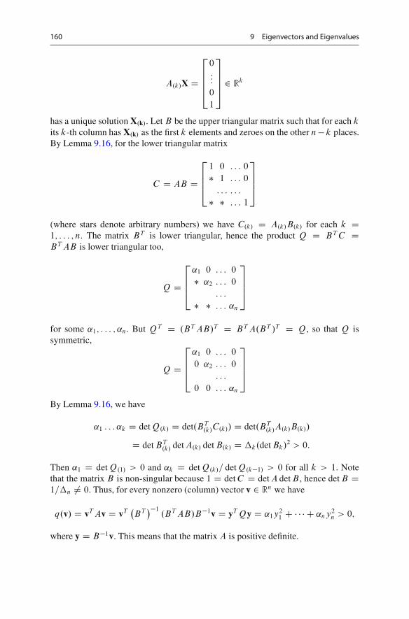
160 9 Eigenvectors and Eigenvalues
A.k/X D
2
6664
0:::
0
1
3
77752 Rk
has a unique solution X.k/. Let B be the upper triangular matrix such that for each k
its k-th column has X.k/ as the first k elements and zeroes on the other n�k places.By Lemma 9.16, for the lower triangular matrix
C D AB D
2
664
1 0 : : : 0
� 1 : : : 0
: : : : : :
� � : : : 1
3
775
(where stars denote arbitrary numbers) we have C.k/ D A.k/B.k/ for each k D1; : : : ; n. The matrix BT is lower triangular, hence the product Q D BT C DBT AB is lower triangular too,
Q D
2
664
˛1 0 : : : 0
� ˛2 : : : 0
: : :
� � : : : ˛n
3
775
for some ˛1; : : : ; ˛n. But QT D .BT AB/T D BT A.BT /T D Q, so that Q issymmetric,
Q D
2
664
˛1 0 : : : 0
0 ˛2 : : : 0
: : :
0 0 : : : ˛n
3
775
By Lemma 9.16, we have
˛1 : : : ˛k D det Q.k/ D det.BT.k/C.k// D det.BT
.k/A.k/B.k//
D det BT.k/ det A.k/ det B.k/ D k.det Bk/2 > 0:
Then ˛1 D det Q.1/ > 0 and ˛k D det Q.k/= det Q.k�1/ > 0 for all k > 1. Notethat the matrix B is non-singular because 1 D det C D det A det B , hence det B D1= n ¤ 0. Thus, for every nonzero (column) vector v 2 Rn we have
q.v/ D vT Av D vT�BT��1
.BT AB/B�1v D yT Qy D ˛1y21 C � � � C ˛ny2
n > 0;
where y D B�1v. This means that the matrix A is positive definite.
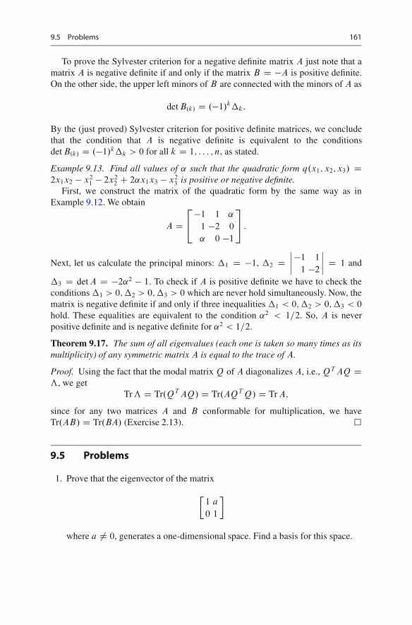
9.5 Problems 161
To prove the Sylvester criterion for a negative definite matrix A just note that amatrix A is negative definite if and only if the matrix B D �A is positive definite.On the other side, the upper left minors of B are connected with the minors of A as
det B.k/ D .�1/k k:
By the (just proved) Sylvester criterion for positive definite matrices, we concludethat the condition that A is negative definite is equivalent to the conditionsdet B.k/ D .�1/k k > 0 for all k D 1; : : : ; n, as stated.
Example 9.13. Find all values of ˛ such that the quadratic form q.x1; x2; x3/ D2x1x2 � x2
1 � 2x22 C 2˛x1x3 � x2
3 is positive or negative definite.First, we construct the matrix of the quadratic form by the same way as in
Example 9.12. We obtain
A D2
4�1 1 ˛
1 �2 0
˛ 0 �1
3
5 :
Next, let us calculate the principal minors: 1 D �1, 2 Dˇˇˇ�1 1
1 �2
ˇˇˇ D 1 and
3 D det A D �2˛2 � 1. To check if A is positive definite we have to check theconditions 1 > 0; 2 > 0; 3 > 0 which are never hold simultaneously. Now, thematrix is negative definite if and only if three inequalities 1 < 0; 2 > 0; 3 < 0
hold. These equalities are equivalent to the condition ˛2 < 1=2. So, A is neverpositive definite and is negative definite for ˛2 < 1=2.
Theorem 9.17. The sum of all eigenvalues (each one is taken so many times as itsmultiplicity) of any symmetric matrix A is equal to the trace of A.
Proof. Using the fact that the modal matrix Q of A diagonalizes A, i.e., QT AQ Dƒ, we get
Tr ƒ D Tr.QT AQ/ D Tr.AQT Q/ D Tr A;
since for any two matrices A and B conformable for multiplication, we haveTr.AB/ D Tr.BA/ (Exercise 2.13). �
9.5 Problems
1. Prove that the eigenvector of the matrix
�1 a
0 1
�
where a ¤ 0, generates a one-dimensional space. Find a basis for this space.

162 9 Eigenvectors and Eigenvalues
2. Prove that the eigenvectors of the matrix
2
42 2 0
0 2 0
0 0 2
3
5
generate a two-dimensional space and find a basis for this space.3. Find the eigenvalues and eigenvectors of the matrices
(a)
2
41 1 1
0 1 1
0 0 1
3
5 and (b)
2
41 1 0
0 1 1
0 0 1
3
5 :
4. Find all complex eigenvalues and eigenvectors of a linear operator in C2 givenby the matrix �
0 2
�2 0
�:
5. Show that for any matrix A, eigenvalues of AT and A are the same.6. Let L be an n-dimensional space, A be a linear operator in L. Let the
characteristic polynomial associated with the transformation matrix of A haven distinct roots. Show that L has a basis consisting of the eigenvectorsof A.
7. Given
A D�
a1 b1
c1 d1
�and B D
�a2 b2
c2 d2
�;
show that the eigenvalues of AB are the same as the eigenvalues of BA.8. Find the eigenvalues of the matrices
(a)
�2 �1
�1 2
�and (b)
�1 1
1 0
�:
9. Let
A D
2
6664
�1 0 : : : 0
0 �2 : : : 0:::
:::: : :
:::
0 0 : : : �n
3
7775
with �i � 0 for all i D 1; : : : ; n. Show that there exists an n� n matrix B suchthat B2 D A.
10. Diagonalize the matrices
(a)
2
4�1 3 �1
�3 5 �1
�3 3 1
3
5 and (b)
2
664
1 1 1 1
1 1 �1 �1
1 �1 1 �1
1 �1 �1 1
3
775 :
9.5 Problems 163
11. Find the eigenvalues and eigenvector of the linear operator d=dt in the space ofpolynomials of degree at most n with real coefficients.
12. Let A be a linear operator in a linear space L. Let L1 be a subspace of Lconsisting of all linear combinations of the eigenvectors of A. Prove that L1
is invariant with respect to A.13. Show that the angle between any two vectors does not change under orthogonal
operator.14. (a) Construct the matrix of the bilinear form �.x; y/ D .x; 2y/� 4x1y2, where
x D .x1; x2/ and y D .y1; y2/ are two vectors in R2, in the basis fu D.0;�1/ ; v D .1; 2/g.
(b) Find the correspondent quadratic form and construct its matrix in the samebasis u; v.
15. Find the values of a; b and c such that the quadratic form q.x1; x2; x3/ D ax21C
2x1x2 C bx22 C cx2
3 is positive or negative definite.16. Let E and E 0 be two bases in Rn and let C be the basis transformation matrix
from E to E 0. Suppose that A and A0 be the matrices of the same quadraticform in these two bases. Show that
A0 D C T AC:

•
10Linear Model of Production in a ClassicalSetting
10.1 Introduction
In classic economics the interrelations in production are vital to understand the lawsof production and distribution, and therefore to understand how an economic systemworks. Wassily Leontief1, a Russian born American economist made the greatestcontribution in this line of thought by developing the input/output analysis2.
In order to explore this idea in a simple way consider an economy consistingthree activities: coal mining, electricity generation and truck production. Outputsof these activities are used in the production of others and are also demanded forfinal use, i.e. consumption and/or investment. For example, extracting coal requiresenergy. Part of its energy requirement can be satisfied in house, by using coal togenerate electricity. The rest is obtained from the power plant. The coal mine alsoemploys several trucks to deliver its output. In this setting, this plant is using coal,energy and trucks to produce coal.
We can express this relation as follows
.Coal; Electricity; Truck/! Coal (10.1)
Coal output is used by other plants. Part of it, as was indicated above, used bythe coal mine to produce energy for its own use. Power plant’s thermal units maybe using coal for producing energy. However, truck production may not require coalas an input. Therefore the remaining output is used to satisfy final consumption by
1Wassily Leontief (1906–1999) was born and educated in St. Petersburg. He received his Ph. D.from Berlin University in 1929. He joined the famous Kiel Institute of World Economics in 1927and worked there until 1930. He moved to the USA in 1931; worked at the Harvard University(1932–1975) and New York University (1975–1991). Leontief was awarded with Nobel Prize inEconomics in 1973 for his contribution to input-output analysis.2For a historical survey and review of the contributions of economists to input-output analysissee [17, 18].
F. Aleskerov et al., Linear Algebra for Economists, Springer Texts in Businessand Economics, DOI 10.1007/978-3-642-20570-5 10,© Springer-Verlag Berlin Heidelberg 2011
165
166 10 Linear Model of Production in a Classical Setting
households for heating. For these activities the above relation can be written as
.Coal; Electricity; Truck/! Electricity (10.2)
.Electricity; Truck/! Truck (10.3)
On the other hand, assuming supply of coal is equal to its demand we can thenwrite
Coal Output D Coal used in coal mineCCoal used in energy plantCCoal used by households for heating
(10.4)
The remaining production activities can be defined in a similar way. Electricpower is used to operate the power plant as well as in other production activities.Households also demand electricity for lighting and/or heating. Trucks can be usedfor all commercial activity. However, we may think that they may not be suitable asfamily cars, and therefore they are not demanded for final consumption. Thereforewe can write
Electricity Output D Electricity used in coal mineCElectricity used in power plantCElectricity used in truck plantCHousehold’s consumption of electricity
(10.5)
Truck OutputD Trucks used in coal mineCTrucks used in power plantCTrucks used in truck plant
(10.6)
Let Xij denote the amount of good i demanded by activity j and Di denotehouseholds’ demand. Then (10.4)–(10.6) can be written as
8<
:
X1 D X11 CX12 CD1;
X2 D X21 CX22 CX23 CD2;
X3 D X31 CX32 CX33;
(10.7)
where i D 1; 2; 3 denotes coal, electricity and truck production activities, respec-tively. Notice that in (10.7), based on the explanation given above, X13 and D3 aretaken as equal to zero.
The description of production activity through such input-output relations delin-eates following points:(a) Production of a commodity requires the use of other commodities as inputs. But
as was the case above, a production activity need not use all the commoditiesavailable in the system. (Coal was not an input in truck production)
(b) A commodity may also be demanded as a final product. In the example abovecoal is demanded for heating. Again this may not be true for all commodities.Trucks may be used only for commercial purposes, and not as family cars.

10.1 Introduction 167
Table 10.1 The use of output (in terms of physical quantities)
Sector 1 Sector 2 : : : Sector n Final Demand Total Output
Sector 1 X11 X12 : : : X1n d1 X1
Sector 2 X21 X22 : : : X2n d2 X2
W W W W W WSector n Xn1 Xn2 : : : Xnn dn Xn
Now let us generalize the example given above to an n-sector economy whereeach sector produces only one commodity .Xi / by one production technique. Inother words there is one-to-one correspondence between commodities producedand the techniques used in their production. Therefore in this simple framework,singling out a sector is equivalent to identifying a specific production technique anda particular commodity. In the remainder of this chapter these terms will be usedinterchangeably.
In such economy each sectors output is used either by other sectors as an inputor by households for final demand, i.e. for consumption, investment or exports. InTable 10.1, each row represents the use of the output of the corresponding sector.The first n entities give the inter-industry use of the output, i.e. the amounts allocatedto other sectors as inputs, .Xij /. The entries in the n C 1’th column represents thefinal use (final demand) of the output (such as consumption, investment and exports)of the corresponding sector.
If supply is equal to demand for all commodities, one can write the following setof equations from Table 10.1.
Xi1 CXi2 C � � � CXin C di D Xi; i D 1; 2; : : : ; n: (10.8)
In each equation the sum of first n entities gives the interindustry demand for thecorresponding commodity and di is the final demand.
Let us define the proportion of commodity i used in the production of commodityj by
aij D Xij
Xj
: (10.9)
Then for a given set of output values fX1; X2; : : : ; Xng, (10.8) can be written as3
nX
j D1
aij Xj C di D Xi; i D 1; 2; : : : ; n: (10.10)
3Notice that, in contrast to its row sums, no meaning can be attributed to column sums ofTable 10.1, since columns consists of elements with different units of measurement (for example,coal is measured by tons, electricity by Kwh and trucks by numbers).

168 10 Linear Model of Production in a Classical Setting
Let us assume that input per output ratios, i.e. aij ’s, are constant for allcommodities. Then (10.10) can be written in a more compact form using matricesand vectors, as
AxC d D x; (10.11)
where A D .aij / is an n � n matrix of input coefficients, x is an n � 1 vector ofindustrial output levels and d is an n � 1 vector of final demand.
Let us denote the j -th column of the matrix A by aj ,
aj D
2
66664
a1j
a2j
:::
anj
3
77775
(10.12)
This vector represents the list of inputs used to produce one unit of commodity j
and will give the commodity input requirements of producing one unit of output j .It is conveniently referred to as the production technique for j .
Example 10.1. Consider the following two sector economy. Let the input coeffi-cient matrix A be given as
A D�
0:3 0:7
0:4 0:1
�:
Find the total output of each sector when the final demand is given by
d D�
12
6
�:
By rearranging (10.11) we get
.I � A/x D d
Applying it to the problem above the following two linear equation system isobtained �
0:7X1 � 0:7X2 D 12
�0:4X1 C 0:9X2 D 6
Using Cramer’s rule
X1 D
ˇˇˇˇ12 �0:7
6 0:9
ˇˇˇˇ
ˇˇˇ0:7 �0:7
�0:4 0:9
ˇˇˇ
D 6:6
0:35D 18:86
and
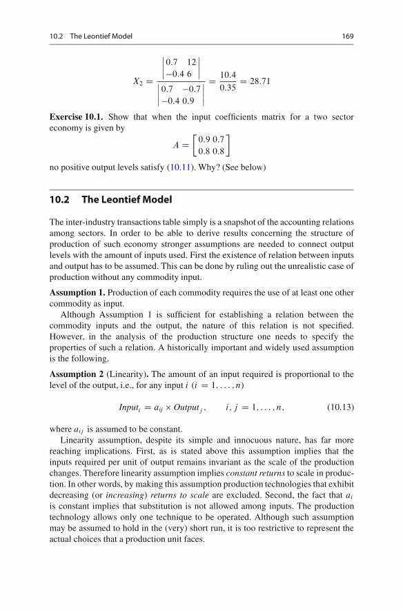
10.2 The Leontief Model 169
X2 D
ˇˇˇ0:7 12
�0:4 6
ˇˇˇ
ˇˇˇ0:7 �0:7
�0:4 0:9
ˇˇˇD 10:4
0:35D 28:71
Exercise 10.1. Show that when the input coefficients matrix for a two sectoreconomy is given by
A D�
0:9 0:7
0:8 0:8
�
no positive output levels satisfy (10.11). Why? (See below)
10.2 The Leontief Model
The inter-industry transactions table simply is a snapshot of the accounting relationsamong sectors. In order to be able to derive results concerning the structure ofproduction of such economy stronger assumptions are needed to connect outputlevels with the amount of inputs used. First the existence of relation between inputsand output has to be assumed. This can be done by ruling out the unrealistic case ofproduction without any commodity input.
Assumption 1. Production of each commodity requires the use of at least one othercommodity as input.
Although Assumption 1 is sufficient for establishing a relation between thecommodity inputs and the output, the nature of this relation is not specified.However, in the analysis of the production structure one needs to specify theproperties of such a relation. A historically important and widely used assumptionis the following.
Assumption 2 (Linearity). The amount of an input required is proportional to thelevel of the output, i.e., for any input i (i D 1; : : : ; n)
Inputi D aij � Outputj ; i; j D 1; : : : ; n; (10.13)
where aij is assumed to be constant.Linearity assumption, despite its simple and innocuous nature, has far more
reaching implications. First, as is stated above this assumption implies that theinputs required per unit of output remains invariant as the scale of the productionchanges. Therefore linearity assumption implies constant returns to scale in produc-tion. In other words, by making this assumption production technologies that exhibitdecreasing (or increasing) returns to scale are excluded. Second, the fact that ai
is constant implies that substitution is not allowed among inputs. The productiontechnology allows only one technique to be operated. Although such assumptionmay be assumed to hold in the (very) short run, it is too restrictive to represent theactual choices that a production unit faces.

170 10 Linear Model of Production in a Classical Setting
Assumption 3 (No Joint Production). Each production technique produces only oneoutput.
One other assumption implicit in the above framework is the absence of jointproduction. This means each production technique produces only one commodity.In reality this may not be the case. Consider a petroleum refinery. Refining crude oilis a technique that leads to multiple oil products, various types of fuel and liquid gas.In this case, the production technique can not be labelled by referring to a specificproduct. In this chapter we shall not deal with the problem of joint production4.
In terms of the symbols used in Table 10.1, (10.13) can be rewritten as
aij D Xij =Xi :
Obviously, aij � 0.Under the assumptions (1)–(3), the production system characterized by (10.11)
satisfies the following conditions:(a) All elements of the A matrix are non-negative, i.e., aij � 0 and for all j there
exists some i , such that aij > 0.(b) Each commodity is produced only with one production technique, i.e. A is a
square matrix.(c) There is no joint production.(d) There are constant returns to scale for all production techniques, i.e. A remains
unchanged when the output vector x changes.Note that the conditions (a) and (b) simply mean that A is a non-negative square
matrix.It is rather easy to show that such system has a unique solution. Due to (b) each
commodity can be characterized by its production technique, i.e. the column vectorof A that corresponds to the commodity in question. Since commodities are distinct,so are their corresponding production techniques. In addition, one can also assumein generic case that the columns of A are linearly independent. Therefore A has fullrank, so .I � A/�1 exists, and by definition is unique. Then the solution to (10.11)is given by
x D .I �A/�1d;
i.e., when the final demand vector is given, it is possible to calculate the output levelsthat enables the system to satisfy it.
It is clear that output level has non-negative value. A production unit can decideto produce the commodity in question (i.e., xi > 0) or may quit production (i.e.,xi D 0). Negative output level has no economic meaning in this framework.Does (10.8) and the assumptions that characterize input coefficients matrix A
guarantee such economically meaningful solution? The answer is no. In order tosee why, consider the following
4See [16, 22] for the discussion of joint production.
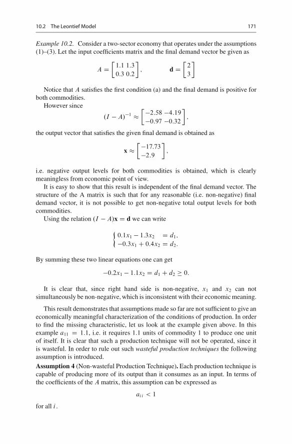
10.2 The Leontief Model 171
Example 10.2. Consider a two-sector economy that operates under the assumptions(1)–(3). Let the input coefficients matrix and the final demand vector be given as
A D�
1:1 1:3
0:3 0:2
�; d D
�2
3
�
Notice that A satisfies the first condition (a) and the final demand is positive forboth commodities.
However since
.I � A/�1 ���2:58 �4:19
�0:97 �0:32
�;
the output vector that satisfies the given final demand is obtained as
x ���17:73
�2:9
�;
i.e. negative output levels for both commodities is obtained, which is clearlymeaningless from economic point of view.
It is easy to show that this result is independent of the final demand vector. Thestructure of the A matrix is such that for any reasonable (i.e. non-negative) finaldemand vector, it is not possible to get non-negative total output levels for bothcommodities.
Using the relation .I �A/x D d we can write
�0:1x1 � 1:3x2 D d1;
�0:3x1 C 0:4x2 D d2:
By summing these two linear equations one can get
�0:2x1 � 1:1x2 D d1 C d2 � 0:
It is clear that, since right hand side is non-negative, x1 and x2 can notsimultaneously be non-negative, which is inconsistent with their economic meaning.
This result demonstrates that assumptions made so far are not sufficient to give aneconomically meaningful characterization of the conditions of production. In orderto find the missing characteristic, let us look at the example given above. In thisexample a11 D 1:1, i.e. it requires 1.1 units of commodity 1 to produce one unitof itself. It is clear that such a production technique will not be operated, since itis wasteful. In order to rule out such wasteful production techniques the followingassumption is introduced.
Assumption 4 (Non-wasteful Production Technique). Each production technique iscapable of producing more of its output than it consumes as an input. In terms ofthe coefficients of the A matrix, this assumption can be expressed as
aii < 1
for all i .

172 10 Linear Model of Production in a Classical Setting
Although this assumption makes a logical point clear, it does not rule out thepossibility that a sector may not be capable of supplying the amount of outputrequired in producing other commodities and/or satisfying the final demand.
It is clear from (10.8) that the surplus output (i.e. the amount of output whichis not consumed as input in its own production) should be sufficient to satisfy inputrequirements of the other sector and the final demand. In other words, the productionsystem should be capable of produce at least as much as it uses as inputs. Non-wastefulness, although necessary, is not sufficient for guaranteeing such outcome.A stronger condition on the production structure is required. This is achieved byintroducing a new assumption based on the following definition.
Definition 10.1. A non-negative matrix A is called productive if there exist x > 0such that
x > Ax:
If the input coefficients matrix is productive, then the corresponding productionsystem AxC d D x is also called productive.
Assumption 5. Input coefficients matrix A is productive.
The five assumptions made thus far are sufficient to characterize a productionsystem that is capable of giving economically meaningful results.
Definition 10.2 (Leontief model). A production system
AxC d D x (10.14)
that satisfies the following assumptions:(a) All the elements of the A matrix are non-negative, i.e. aij � 0 and for all j
there exists some i such that aij > 0.(b) Each commodity is produced only with one production technique, i.e. A is a
square matrix.(c) There is no joint production.(d) There are constant returns to scale for all production techniques, i.e. A remains
unchanged when the output vector x changes.(e) A is productive.is called the Leontief model.
10.3 Existence of a Unique Non-Negative Solutionto the Leontief System
The purpose of this section is to demonstrate that for any d � 0 it is possible to geta unique non-negative solution to the Leontief system.
In order to prove the existence and uniqueness of a non-negative solution to aLeontief model when the input coefficients matrix is productive, we shall provesome mathematical results that are needed to prove the main proposition. Theseresults are given as lemmas below.
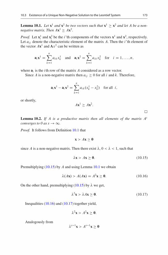
10.3 Existence of a Unique Non-Negative Solution to the Leontief System 173
Lemma 10.1. Let x1 and x2 be two vectors such that x1 � x2 and let A be a non-negative matrix. Then Ax1 � Ax2.
Proof. Let x1i and x2
i be the i ’th components of the vectors x1 and x2, respectively.Let aij denote the characteristic element of the matrix A. Then the i ’th element ofthe vector Ax1 and Ax2 can be written as
aix1 DnX
kD1
aikx1k and ai x2 D
nX
kD1
aikx2k for i D 1; : : : ; n;
where ai is the i th row of the matrix A considered as a row vector.Since A is a non-negative matrix then aij � 0 for all i and k. Therefore,
ai x1 � ai x2 DnX
kD1
aik.x1k � x2
k/ for all i;
or shortly,Ax1 � Ax2:
�
Lemma 10.2. If A is a productive matrix then all elements of the matrix As
converges to 0 as s !1.
Proof. It follows from Definition 10.1 that
x > Ax � 0
since A is a non-negative matrix. Then there exist �, 0 < � < 1, such that
�x > Ax � 0: (10.15)
Premultiplying (10.15) by A and using Lemma 10.1 we obtain
�.Ax/ > A.Ax/ D A2x � 0: (10.16)
On the other hand, premultiplying (10.15) by � we get,
�2x > �Ax � 0: (10.17)
Inequalities (10.16) and (10.17) together yield,
�2x > A2x � 0:
Analogously from�s�1x > As�1x � 0
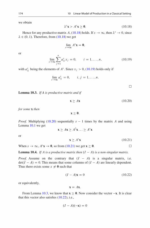
174 10 Linear Model of Production in a Classical Setting
we obtain�sx > Asx � 0: (10.18)
Hence for any productive matrix A, (10.18) holds. If s !1, then �s ! 0, since� 2 .0; 1/. Therefore, from (10.18) we get
lims!1 Asx D 0;
or
lims!1
nX
j D1
asij xj D 0; i D 1; : : : ; n; (10.19)
with asij being the elements of As . Since xj > 0, (10.19) holds only if
lims!1 as
ij D 0; i; j D 1; : : : ; n:
�
Lemma 10.3. If A is productive matrix and if
x � Ax (10.20)
for some x thenx � 0:
Proof. Multiplying (10.20) sequentially s � 1 times by the matrix A and usingLemma 10.1 we get
x � Ax � A2x : : : � Asx
orx � Asx (10.21)
When s !1, Asx! 0, so from (10.21) we get x � 0. �
Lemma 10.4. If A is a productive matrix then .I � A/ is a non-singular matrix.
Proof. Assume on the contrary that .I � A/ is a singular matrix, i.e.det.I � A/ D 0. This means that some columns of .I � A/ are linearly dependent.Thus there exists some x 6D 0 such that
.I � A/x D 0 (10.22)
or equivalently,x D Ax:
From Lemma 10.3, we know that x � 0. Now consider the vector �x. It is clearthat this vector also satisfies (10.22), i.e.,
.I � A/.�x/ D 0

10.3 Existence of a Unique Non-Negative Solution to the Leontief System 175
Again from Lemma 10.3, it must be true that �x � 0. The inequalities �x � 0and �x � 0 can jointly be satisfied only if x D 0, which is in contradiction withx 6D 0. �
The preceding four lemmas allows us to prove the following theorem showingthat a Leontief model has a unique non-negative solution.
Theorem 10.5. Given any non-negative d, the system
.I � A/x D d (10.23)
has a unique non-negative solution if the matrix A is productive.
Proof. Let A be a productive matrix. Take any d � 0 and consider the equa-tion (10.23).
By Lemma 10.4, .I �A/ is not singular, since A is productive. So, (10.23) has aunique solution Qx. It is also true that
.I �A/Qx � 0:
since d � 0. Then by Lemma 10.3 we get Qx � 0.Now, assume that the system (10.23) has a non-negative solution x for some
d > 0 and some A. Then x� Ax D .I �A/x D d > 0, that is, A is productive. �
Remark 10.1. Notice that the productivity of A is not necessary to get a non-negative solution to (10.23). For example, for d D 0 this system has a solutionx D 0 for any matrix A. However, if d > 0, then a non-negative solution x exists ifand only if the matrix A is productive (because we have x D AxC d > Ax, that is,the productivity condition holds).
Another criterion (the Hawkins-Simon condition) can be derived from thefollowing theorem.
Theorem 10.6. Let A be a non-negative matrix. Then the following conditions areequivalent:
i. A is productive;ii. the matrix .I �A/�1 exists and is non-negative;
iii. all successive principal minors of B D I �A are positive.
In the last condition, these principal minors are
B.1/ D b11 > 0;
B.2/ Dˇˇˇˇb11 b12
b21 b22
ˇˇˇˇ > 0;
: : :
B.n/ D
ˇˇˇˇˇ
b11 : : : b1n
:::: : :
:::
bn1 : : : bnn
ˇˇˇˇˇ
> 0:
176 10 Linear Model of Production in a Classical Setting
The condition (iii) is called Hawkins–Simon condition. The equivalence of thiscondition (iii) and the condition (ii) of productivity of A is called Hawkins–Simontheorem [12].
Proof. Let us first prove that the condition (i) implies (ii). Suppose that A isproductive. Then the matrix .I �A/�1 exists by Lemma 10.4. Let us define
‰s D I CAC A2 C A3 C : : :C As;
thenA‰s D AC A2 C A3 C : : :C AsC1:
Therefore.I � A/‰s D I �AsC1:
Taking the limit of both sides as s !1 one gets
lims!1Œ.I �A/‰s� D I
since AsC1 ! 0 as s !1, by Lemma 10.2. Therefore,
‰s D I C AC A2 C A3 C : : :C As �! .I � A/�1;
and since A � 0, we have ‰s > 0 and
.I �A/�1 � 0:
Now let us show that (ii) implies (i). Assume that .I � A/�1 � 0. Take anyd > 0 (e. g., d D .1; : : : ; 1/). Then the system .I � A/x D d has a unique solutionx D .I � A/�1d � 0. By the Remark after Theorem 10.5, it follows that A isproductive.
For the equivalence of Hawkins–Simon condition (iii) and the productivitycondition (i), see, for example5, [30, pp. 384–385]. Another proof based oneconomic intuition is given in [6]. �
10.4 Conditions for Getting a Positive (EconomicallyMeaningful) Solution to the Leontief Model
For practical purposes if a commodity is not demanded and supplied it can beomitted. In other words, an economically meaningful solution to a Leontief modelshould be the one that assigns positive output levels for all commodities, even when
5In [21], O’Neill & Wood dropped the continuity assumption and proved theorem by assumingcolumn sums of B are not greater than one. The latter assumption can be fulfilled in practice byappropriately choosing the measurement units for each commodity.
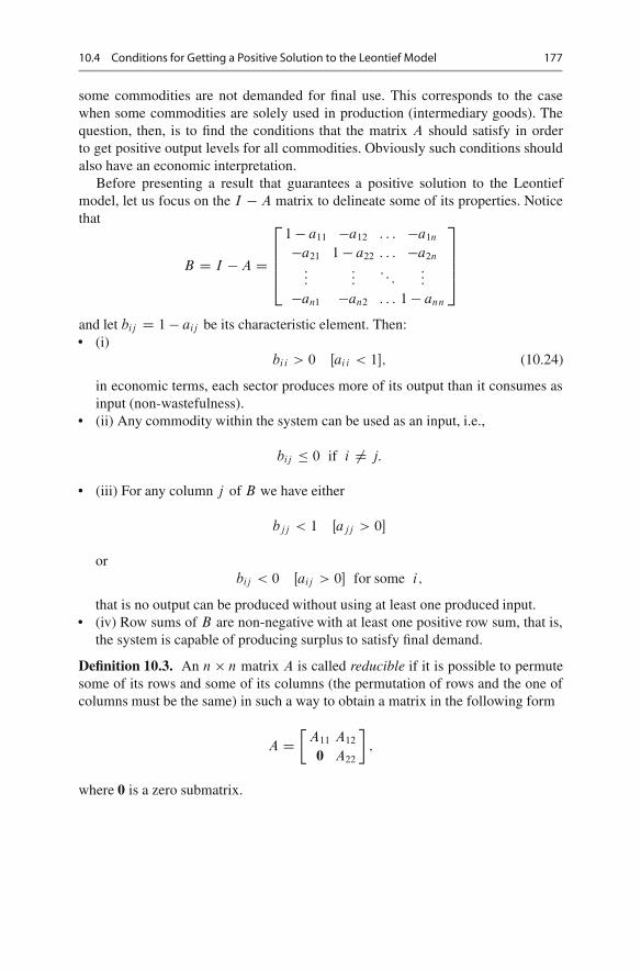
10.4 Conditions for Getting a Positive Solution to the Leontief Model 177
some commodities are not demanded for final use. This corresponds to the casewhen some commodities are solely used in production (intermediary goods). Thequestion, then, is to find the conditions that the matrix A should satisfy in orderto get positive output levels for all commodities. Obviously such conditions shouldalso have an economic interpretation.
Before presenting a result that guarantees a positive solution to the Leontiefmodel, let us focus on the I � A matrix to delineate some of its properties. Noticethat
B D I �A D
2
6664
1 � a11 �a12 : : : �a1n
�a21 1 � a22 : : : �a2n
::::::
: : ::::
�an1 �an2 : : : 1 � ann
3
7775
and let bij D 1 � aij be its characteristic element. Then:• (i)
bii > 0 Œai i < 1�; (10.24)
in economic terms, each sector produces more of its output than it consumes asinput (non-wastefulness).
• (ii) Any commodity within the system can be used as an input, i.e.,
bij � 0 if i 6D j:
• (iii) For any column j of B we have either
bjj < 1 Œajj > 0�
orbij < 0 Œaij > 0� for some i;
that is no output can be produced without using at least one produced input.• (iv) Row sums of B are non-negative with at least one positive row sum, that is,
the system is capable of producing surplus to satisfy final demand.
Definition 10.3. An n � n matrix A is called reducible if it is possible to permutesome of its rows and some of its columns (the permutation of rows and the one ofcolumns must be the same) in such a way to obtain a matrix in the following form
A D�
A11 A12
0 A22
�;
where 0 is a zero submatrix.
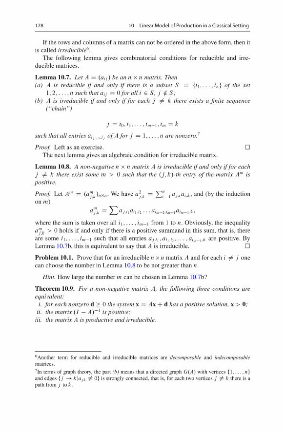
178 10 Linear Model of Production in a Classical Setting
If the rows and columns of a matrix can not be ordered in the above form, then itis called irreducible6.
The following lemma gives combinatorial conditions for reducible and irre-ducible matrices.
Lemma 10.7. Let A D .aij / be an n � n matrix. Then(a) A is reducible if and only if there is a subset S D fi1; : : : ; ing of the set
1; 2; : : : ; n such that aij D 0 for all i 2 S , j … S ;(b) A is irreducible if and only if for each j ¤ k there exists a finite sequence
(“chain”)
j D i0; i1; : : : ; im�1; im D k
such that all entries aij �1;ij of A for j D 1; : : : ; n are nonzero.7
Proof. Left as an exercise. �The next lemma gives an algebraic condition for irreducible matrix.
Lemma 10.8. A non-negative n � n matrix A is irreducible if and only if for eachj ¤ k there exist some m > 0 such that the .j; k/-th entry of the matrix Am ispositive.
Proof. Let Am D .amj;k/n�n. We have a2
j;k DPn
iD1 aj;i ai;k , and (by the inductionon m)
amj;k D
Xaj;i1ai1;i2 : : : aim�2;im�1aim�1;k;
where the sum is taken over all i1; : : : ; im�1 from 1 to n. Obviously, the inequalityam
j;k > 0 holds if and only if there is a positive summand in this sum, that is, thereare some i1; : : : ; im�1 such that all entries aj;i1 ; ai1;i2 ; : : : ; aim�1;k are positive. ByLemma 10.7b, this is equivalent to say that A is irreducible. �Problem 10.1. Prove that for an irreducible n�n matrix A and for each i ¤ j onecan choose the number in Lemma 10.8 to be not greater than n.
Hint. How large the number m can be chosen in Lemma 10.7b?
Theorem 10.9. For a non-negative matrix A, the following three conditions areequivalent:
i. for each nonzero d � 0 the system x D AxC d has a positive solution, x > 0;ii. the matrix .I �A/�1 is positive;
iii. the matrix A is productive and irreducible.
6Another term for reducible and irreducible matrices are decomposable and indecomposablematrices.7In terms of graph theory, the part (b) means that a directed graph G.A/ with vertices f1; : : : ; ngand edges fj ! kjajk ¤ 0g is strongly connected, that is, for each two vertices j ¤ k there is apath from j to k.
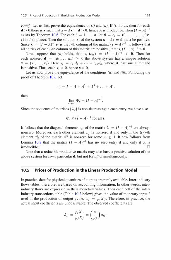
10.5 Prices of Production in the Linear Production Model 179
Proof. Let us first prove the equivalence of (i) and (ii). If (i) holds, then for eachd > 0 there is x such that x � Ax D d > 0, hence A is productive. Then .I � A/�1
exists by Theorem 10.6. For each i D 1; : : : ; n, let d D ei D .0; : : : ; 1; : : : ; 0/T
(1 in i -th place). Then the solution xi of the system x � Ax D d must be positive.Since xi D .I � A/�1ei is the i -th column of the matrix .I � A/�1, it follows thatall entries of each i -th column of this matrix are positive, that is, .I � A/�1 > 0.
Now, suppose that (ii) holds, that is, .cij / D .I � A/�1 > 0. Then foreach nonzero d D .d1; : : : ; dn/ � 0 the above system has a unique solutionx D .x1; : : : ; xn/: Here xi D ci1d1 C � � � C cindn, where at least one summandis positive. Thus, each xi > 0, hence x > 0.
Let us now prove the equivalence of the conditions (ii) and (iii). Following theproof of Theorem 10.6, let
‰s D I CAC A2 C A3 C : : :C As I
thenlim
s!1 ‰s D .I � A/�1:
Since the sequence of matrices f‰sg is non-decreasing in each entry, we have also
‰s � .I � A/�1 for all s:
It follows that the diagonal elements ci i of the matrix C D .I � A/�1 are alwaysnonzero. Moreover, each other element cij is nonzero if and only if the .ij /-thelement ak
ij of the matrix Am is nonzero for some m � 1. It now follows fromLemma 10.8 that the matrix .I � A/�1 has no zero entry if and only if A isirreducible. �
Note that a reducible productive matrix may also have a positive solution of theabove system for some particular d, but not for all d simultaneously.
10.5 Prices of Production in the Linear Production Model
In practice, data for physical quantities of outputs are rarely available. Inter-industryflows tables, therefore, are based on accounting information. In other words, inter-industry flows are expressed in their monetary values. Then each cell of the inter-industry transactions table (Table 10.2 below) gives the value of monetary input i
used in the production of output j , i.e. vij D pi Xij . Therefore, in practice, theactual input coefficients are unobservable. The observed coefficients are
Qaij D piXij
pj Xj
D�
pi
pj
�aij ;
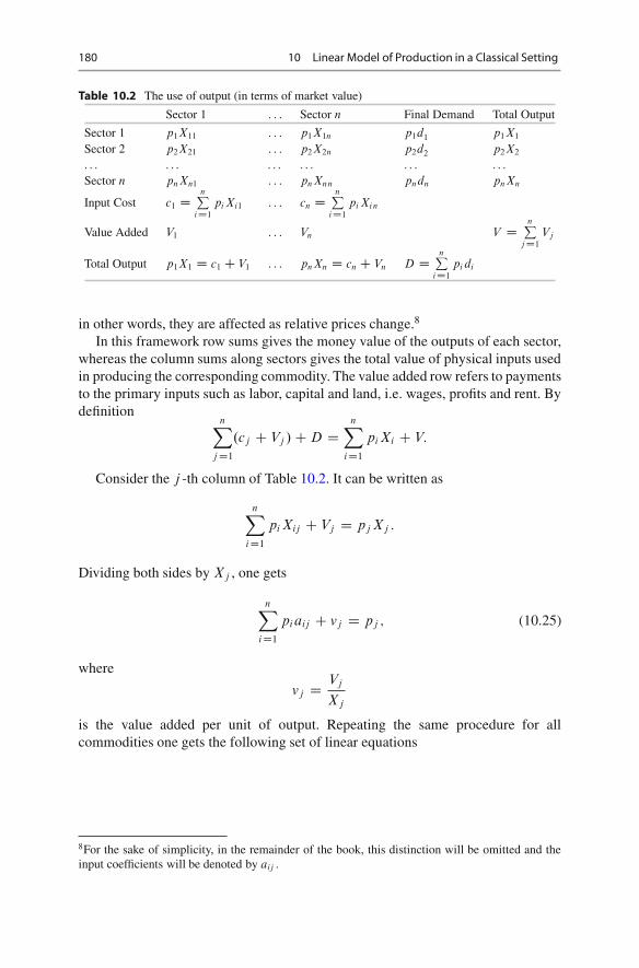
180 10 Linear Model of Production in a Classical Setting
Table 10.2 The use of output (in terms of market value)
Sector 1 : : : Sector n Final Demand Total Output
Sector 1 p1X11 : : : p1X1n p1d1 p1X1
Sector 2 p2X21 : : : p2X2n p2d2 p2X2
. . . . . . . . . . . . . . . . . .Sector n pnXn1 : : : pnXnn pndn pnXn
Input Cost c1 D nP
iD1
pi Xi1 : : : cn D nP
iD1
pi Xin
Value Added V1 : : : Vn V DnP
jD1
Vj
Total Output p1X1 D c1 C V1 : : : pnXn D cn C Vn D D nP
iD1
pi di
in other words, they are affected as relative prices change.8
In this framework row sums gives the money value of the outputs of each sector,whereas the column sums along sectors gives the total value of physical inputs usedin producing the corresponding commodity. The value added row refers to paymentsto the primary inputs such as labor, capital and land, i.e. wages, profits and rent. Bydefinition
nX
j D1
.cj C Vj /CD DnX
iD1
piXi C V:
Consider the j -th column of Table 10.2. It can be written as
nX
iD1
pi Xij C Vj D pj Xj :
Dividing both sides by Xj , one gets
nX
iD1
piaij C vj D pj ; (10.25)
where
vj D Vj
Xj
is the value added per unit of output. Repeating the same procedure for allcommodities one gets the following set of linear equations
8For the sake of simplicity, in the remainder of the book, this distinction will be omitted and theinput coefficients will be denoted by aij .
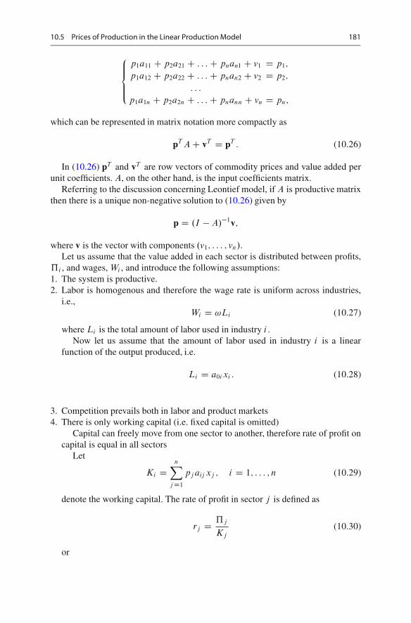
10.5 Prices of Production in the Linear Production Model 181
8ˆ<
ˆ:
p1a11 C p2a21 C : : :C pnan1 C v1 D p1;
p1a12 C p2a22 C : : :C pnan2 C v2 D p2;
: : :
p1a1n C p2a2n C : : :C pnann C vn D pn;
which can be represented in matrix notation more compactly as
pT AC vT D pT : (10.26)
In (10.26) pT and vT are row vectors of commodity prices and value added perunit coefficients. A, on the other hand, is the input coefficients matrix.
Referring to the discussion concerning Leontief model, if A is productive matrixthen there is a unique non-negative solution to (10.26) given by
p D .I � A/�1v;
where v is the vector with components .v1; : : : ; vn/.Let us assume that the value added in each sector is distributed between profits,
…i , and wages, Wi , and introduce the following assumptions:1. The system is productive.2. Labor is homogenous and therefore the wage rate is uniform across industries,
i.e.,Wi D !Li (10.27)
where Li is the total amount of labor used in industry i .Now let us assume that the amount of labor used in industry i is a linear
function of the output produced, i.e.
Li D a0i xi : (10.28)
3. Competition prevails both in labor and product markets4. There is only working capital (i.e. fixed capital is omitted)
Capital can freely move from one sector to another, therefore rate of profit oncapital is equal in all sectors
Let
Ki DnX
j D1
pj aij xj ; i D 1; : : : ; n (10.29)
denote the working capital. The rate of profit in sector j is defined as
rj D …j
Kj
(10.30)
or
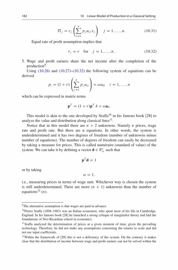
182 10 Linear Model of Production in a Classical Setting
…j D rj
nX
iD1
pj aij xj
!
j D 1; : : : ; n: (10.31)
Equal rate of profit assumption implies that
rj D r for j D 1; : : : ; n: (10.32)
5. Wage and profit earners share the net income after the completion of theproduction9.Using (10.26) and (10.27)–(10.32) the following system of equations can be
derived
pi D .1C r/
0
@nX
j D1
pj aij
1
AC !a0i i D 1; : : : ; n
which can be expressed in matrix terms
pT D .1C r/pT AC !a0:
This model is akin to the one developed by Sraffa10 in his famous book [28] toanalyze the value and distribution along classical lines11.
Notice that in this model there are n C 2 unknowns. Namely n prices, wagerate and profit rate. But there are n equations. In other words, the system isunderdetermined and it has two degrees of freedom (number of unknowns minusnumber of equations). The number of degrees of freedom can easily be decreasedby taking a measure for prices. This is called numeraire (standard of value) of thesystem. We can take it by defining a vector d 2 RnC such that
pT d D 1
or by taking! D 1;
i.e., measuring prices in terms of wage unit. Whichever way is chosen the systemis still underdetermined. There are more (n C 1) unknowns than the number ofequations12 (n).
9The alternative assumption is that wages are paid in advance.10Pierro Sraffa (1898–1983) was an Italian economist, who spent most of his life in Cambridge,England. In his famous book [28] he launched a strong critique of marginalist theory and laid thefoundations of Neo-Ricardian school in economics.11Sraffa analyzed the determination of prices at a given moment of time, given the prevailingtechnology. Therefore, he did not make any assumptions concerning the returns to scale and didnot use input coefficients.12Within the framework of [28] this is not a deficiency of the system. On the contrary it makesclear that the distribution of income between wage and profit earners can not be solved within the
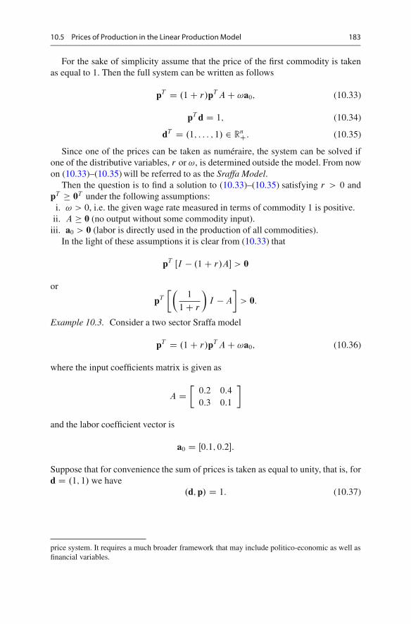
10.5 Prices of Production in the Linear Production Model 183
For the sake of simplicity assume that the price of the first commodity is takenas equal to 1. Then the full system can be written as follows
pT D .1C r/pT AC !a0; (10.33)
pT d D 1; (10.34)
dT D .1; : : : ; 1/ 2 RnC: (10.35)
Since one of the prices can be taken as numeraire, the system can be solved ifone of the distributive variables, r or !, is determined outside the model. From nowon (10.33)–(10.35) will be referred to as the Sraffa Model.
Then the question is to find a solution to (10.33)–(10.35) satisfying r > 0 andpT � 0T under the following assumptions:
i. ! > 0, i.e. the given wage rate measured in terms of commodity 1 is positive.ii. A � 0 (no output without some commodity input).
iii. a0 > 0 (labor is directly used in the production of all commodities).In the light of these assumptions it is clear from (10.33) that
pT ŒI � .1C r/A� > 0
or
pT
��1
1C r
�I �A
�> 0:
Example 10.3. Consider a two sector Sraffa model
pT D .1C r/pT AC !a0; (10.36)
where the input coefficients matrix is given as
A D�
0:2 0:4
0:3 0:1
�
and the labor coefficient vector is
a0 D Œ0:1; 0:2�:
Suppose that for convenience the sum of prices is taken as equal to unity, that is, ford D .1; 1/ we have
.d; p/ D 1: (10.37)
price system. It requires a much broader framework that may include politico-economic as well asfinancial variables.

184 10 Linear Model of Production in a Classical Setting
i. Find the relation between wage rate and the rate of profit (wage-profit trade-off)for this economy.
ii. Calculate the prices in terms of the numeraire.
Solution. i. Notice for any 0 < r < 1 the matrix .1 C r/AT is productive(by Hawkins–Simon conditions, see Theorem 10.6) and positive, hence by Theo-rem 10.9 the matrix .I � .1C r/A/�1 exists and is positive.13
By (10.36), we have
pT D !a0 .I � .1C r/A/�1 : (10.38)
Using (10.37), we get
1 D pT dT D !a0 .I � .1C r/A/�1 dT ;
thus,
! D 1
a0 .I � .1C r/A/�1 dT: (10.39)
Notice that (10.39) indicates a trade-off between r and w. An increase in the rate ofprofit leads to a decline in the wage rate. Substituting the given numerical values,we have
! D 1
Œ0:1; 0:2�
�1� 0:2.1C r/ �0:4.1C r/
�0:3.1C r/ 1 � 0:1.1C r/
��1 �1
1
� D 26 � 5r � r2
7C r:
ii. Substituting (10.39) in (10.38) one gets
pT D 1
a0 .I � .1C r/A/�1 dTa0 .I � .1C r/A/�1 D
�3C r
7C r;
4
7C r
�: (10.40)
Notice that (10.39) and (10.40) are in general non-linear.
10.6 Perron–Frobenius Theorem
In this section another mathematical tool that can be used to find a economicallymeaningful solution to (10.33) is introduced. It is based on better understanding ofeigenvectors and eigenvalues of non-negative matrices (recall that we have discussedeigenvectors and eigenvalues in general in Chap. 9). We are interested in non-
13For r � 1 the matrix .1 C r/A is not productive (again by Hawkins–Simon conditions), so, theproblem has no economical sense.
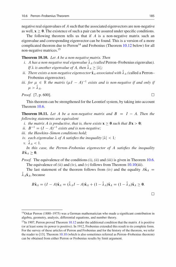
10.6 Perron–Frobenius Theorem 185
negative real eigenvalues of A such that the associated eigenvectors are non-negativeas well, x � 0. The existence of such a pair can be assured under specific conditions.
The following theorem tells us that if A is a non-negative matrix such aneigenvalue and corresponding eigenvector can be found. This is a version of a morecomplicated theorem due to Perron14 and Frobenius (Theorem 10.12 below) for allnon-negative matrices.15
Theorem 10.10. Let A be a non-negative matrix. Theni. A has a non-negative real eigenvalue O�A (called Perron–Frobenius eigenvalue).
If � is another eigenvalue of A, then O�A � j�j;ii. There exists a non-negative eigenvector OxA associated with O�A (called a Perron–
Frobenius eigenvector).iii. for � 2 R the matrix .�I � A/�1 exists and is non-negative if and only if
� > O�A.
Proof. [7, p. 600]. �This theorem can be strengthened for the Leontief system, by taking into account
Theorem 10.6.
Theorem 10.11. Let A be a non-negative matrix and B D I � A. Then thefollowing statements are equivalent
i. the matrix A is productive, that is, there exists x � 0 such that Bx > 0;ii. B�1 D .I � A/�1 exists and is non-negative;
iii. the Hawkins–Simon conditions hold;iv. each eigenvalue � of A satisfies the inequality j�j < 1;v. O�A < 1.
In this case, the Perron–Frobenius eigenvector of A satisfies the inequalityB OxA � 0.
Proof. The equivalence of the conditions (i), (ii) and (iii) is given in Theorem 10.6.The equivalence of (ii) and (iv), and (v) follows from Theorem 10.10(iii).The last statement of the theorem follows from (iv) and the equality AOxA D
O�A OxA, because
B OxA D .I � A/OxA D . O�AI �A/OxA C .1 � O�A/OxA D .1 � O�A/OxA � 0:
�
14Oskar Perron (1880–1975) was a German mathematician who made a significant contribution inalgebra, geometry, analysis, differential equations, and number theory.15In 1907, Perron proved Theorem 10.12 under the additional condition that the matrix A is positive(or at least some its power is positive). In 1912, Frobenius extended this result to its complete form.For the survey of these articles of Perron and Frobenius and for the history of the theorem, we referthe reader to [13]. Theorem 10.10 (which is also sometimes referred as Perron–Frobenius theorem)can be obtained from either Perron or Frobenius results by limit argument.
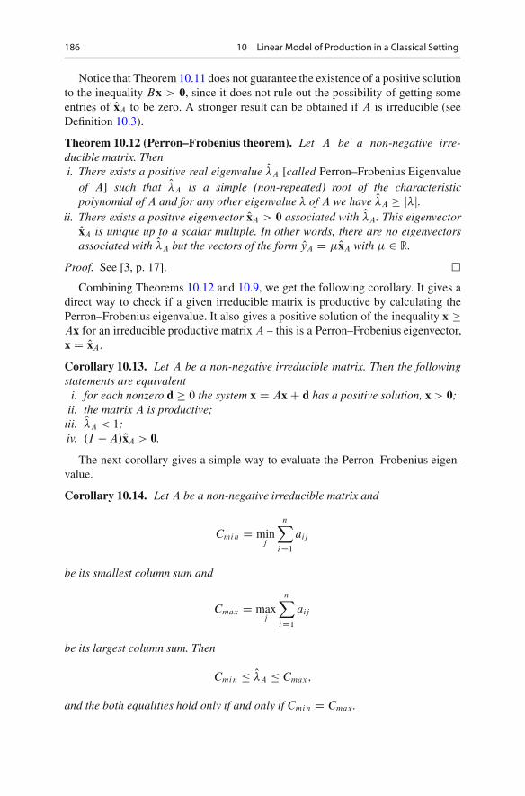
186 10 Linear Model of Production in a Classical Setting
Notice that Theorem 10.11 does not guarantee the existence of a positive solutionto the inequality Bx > 0, since it does not rule out the possibility of getting someentries of OxA to be zero. A stronger result can be obtained if A is irreducible (seeDefinition 10.3).
Theorem 10.12 (Perron–Frobenius theorem). Let A be a non-negative irre-ducible matrix. Theni. There exists a positive real eigenvalue O�A [called Perron–Frobenius Eigenvalue
of A] such that O�A is a simple (non-repeated) root of the characteristicpolynomial of A and for any other eigenvalue � of A we have O�A � j�j.
ii. There exists a positive eigenvector OxA > 0 associated with O�A. This eigenvectorOxA is unique up to a scalar multiple. In other words, there are no eigenvectorsassociated with O�A but the vectors of the form OyA D �OxA with � 2 R.
Proof. See [3, p. 17]. �Combining Theorems 10.12 and 10.9, we get the following corollary. It gives a
direct way to check if a given irreducible matrix is productive by calculating thePerron–Frobenius eigenvalue. It also gives a positive solution of the inequality x �Ax for an irreducible productive matrix A – this is a Perron–Frobenius eigenvector,x D OxA.
Corollary 10.13. Let A be a non-negative irreducible matrix. Then the followingstatements are equivalent
i. for each nonzero d � 0 the system x D AxC d has a positive solution, x > 0;ii. the matrix A is productive;
iii. O�A < 1;iv. .I � A/OxA > 0.
The next corollary gives a simple way to evaluate the Perron–Frobenius eigen-value.
Corollary 10.14. Let A be a non-negative irreducible matrix and
Cmin D minj
nX
iD1
aij
be its smallest column sum and
Cmax D maxj
nX
iD1
aij
be its largest column sum. Then
Cmin � O�A � Cmax;
and the both equalities hold only if and only if Cmin D Cmax.

10.7 Linear Production Model 187
Proof. Let OxA be the eigenvector associated with O�A Then
O�A OxA D AOxA;
which means
O�A OxAi D
nX
j D1
aij OxAj for i D 1; : : : ; n;
where OxAi is the i ’th element of the vector OxA. Summing this expression over i , we
have
O�A
nX
iD1
OxAi D
nX
iD1
nX
j D1
aij OxAj D
nX
j D1
OxAj
nX
iD1
aij ;
which can be written as
O�A DnX
j D1
OxAj
nX
iD1
aij =
nX
iD1
OxAi ;
i.e. O�A can be expressed as a non-negative weighted average of the column sumsof A. �
Remark 10.2. Same result holds for the row sums of A.
10.7 Linear Production Model (continued)
In this section the economic meaning of conditions required to guarantee a positivesolution to (10.25) will be discussed. The discussion is based on a classificationintroduced by Sraffa in [28].
Sraffa makes a distinction between those commodities required directly orindirectly in the production of every commodity (Basic Commodities) and thosethat do not posses such a property (Non-Basic commodities). He demonstrates thatwhile the former type of commodities play a significant role in the determination ofthe rate of profit and prices, the latter has no such influence.
It is clear that a commodity i is directly required in the production of commodityj if and only if
aij > 0:
Now suppose that for a commodity pair .i; j /
aij D 0;
but there exist a commodity k such that

188 10 Linear Model of Production in a Classical Setting
akj > 0 and aik > 0:
In other words, although commodity i does not directly used as an input in theproduction of the commodity j , it is required for the production of k, which is adirect input in producing j . The commodity i is said to be indirectly required inproducing j .
Example 10.4. Let the input coefficient matrix be defined as follows
A D2
4a11 a12 a13
0 a22 a23
a31 a32 a33
3
5
where aij > 0 for all i; j , except a21.Here second commodity is not directly required for the production of the
commodity 1. However in order to produce one unit of commodity 3, a23 > 0
amount of commodity 3 is required. On the other hand a31 > 0 amount ofcommodity 3 is required in order to produce one unit of commodity 1. Therefore,in order to produce one unit of commodity 1, a31a23 amount of commodity 2 isindirectly required.
Now consider the following matrix multiplication
A2 D A � A:
Let the .i; j /’th element of A2 be denoted as a2ij . Then it is easy to see that in the
above example that a21 D a32a31, hence for all i; j
either aij > 0 or a2ij > 0:
This following definition is the generalization of the result obtained in theexample given above.
Definition 10.4. Let A be a non negative input coefficients matrix, whose j -thcolumn is associated with the commodity j . Then j is a basic commodity if forsome k � n
.AC A2 C : : :C Ak/ej > 0; (10.41)
where ej is the unit vector whose j -th component is equal to one.
Theorem 10.15. Consider an economy with n commodities, i D 1; : : : ; n. Let A
be the n � n input coefficients matrix of this economy. Then all commodities in thiseconomy are basic commodities if and only if A is irreducible.
Proof. Note that the inequality (10.41) in Definition 10.4 means that j -th columnof the matrix
AC A2 C : : :C An
is positive.

10.7 Linear Production Model 189
If all commodities are basic, then from Definition 10.4 we get
ACA2 C : : :CAn D .AC A2 C : : :C An/I > 0;
hence for all i and j there is k � n such that akij > 0. Then by Lemma 10.8 A is
irreducible.Now suppose that A is irreducible. Then, by Lemma 10.8 for each i ¤ j
there exist m D m.i; j / such that amij > 0. By Problem 10.1 (the problem after
Lemma 10.8), we may choose m � n.For each i and each j ¤ i , we have
am.i;j /Cm.j;i/i i � a
m.i;j /ij a
m.j;i/j i > 0;
(since Am.i;j /Cm.j;i/ D Am.i;j /Am.j;i/), that is, there exists m > 0 such that amii > 0.
Following the proof of Lemma 10.8, this means that there exists a sequence
i D i0; i1; : : : ; im�1; im D i
of indexes such that all matrix entries aij ;ij C1are nonzero. Consider such a sequence
of minimal length m. There is no repeated elements in it but i0 D im D i , therefore,there are at most n pairwise different elements. Hence m � n.
So, for each i; j the .i; j /-th entry of some matrix Am for 1 � m � n is positive.Hence,
AC A2 C : : :C An > 0:
Thus, each column of the matrix in the left hand side is positive, that is, eachcommodity is basic. �
10.7.1 Sraffa System: The Case of Basic Commodities
Now let us turn to (10.33) and assume that A is irreducible. Then by Theorem 10.12we know that A has a positive Perron–Frobenius eigenvalue and an associatedeigenvector which is also positive. Of course, the same is true for the transposematrix AT .
Let Op be the left Perron–Frobenius eigenvector of A, that is, the Perron–Frobeniuseigenvector of AT . Therefore for O�A > 0 and for the associated price vector OpT > 0we have
OpT O�A D OpT A
orOpT . O�AI �A/ D 0:
It follows that if
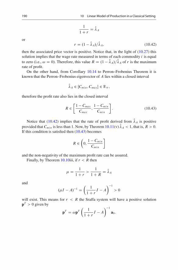
190 10 Linear Model of Production in a Classical Setting
1
1C rD O�A
orr D .1 � O�A/= O�A; (10.42)
then the associated price vector is positive. Notice that, in the light of (10.27) thissolution implies that the wage rate measured in terms of each commodity i is equalto zero (i.e., ! D 0/. Therefore, this value R D .1 � O�A/= O�A of r is the maximumrate of profit.
On the other hand, from Corollary 10.14 to Perron–Frobenius Theorem it isknown that the Perron–Frobenius eigenvector of A lies within a closed interval
O�A 2 ŒCmin; Cmax� 2 RC;
therefore the profit rate also lies in the closed interval
R 2�
1 � Cmax
Cmax
;1 � Cmin
Cmin
�: (10.43)
Notice that (10.42) implies that the rate of profit derived from O�A is positiveprovided that Cmin is less than 1. Now, by Theorem 10.11(v) O�A < 1, that is, R > 0.If this condition is satisfied then (10.43) becomes
R 2�
0;1 � Cmin
Cmin
�
and the non-negativity of the maximum profit rate can be assured.Finally, by Theorem 10.10iii, if r < R then
� D 1
1C r>
1
1CRD O�A
and
.�I � A/�1 D�
1
1C rI � A
��1
> 0
will exist. This means for r < R the Sraffa system will have a positive solutionpT > 0 given by
pT D !pT
�1
1C rI �A
��1
a0:
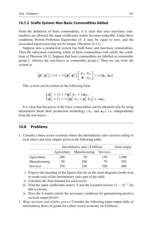
10.8 Problems 191
10.7.2 Sraffa System: Non-Basic Commodities Added
From the definition of basic commodities, it is clear that once non-basic com-modities are allowed, the input coefficients matrix becomes reducible. Under theseconditions Perron–Frobenius Eigenvalue of A may be equal to zero, and theassociated eigenvector may not be unique (Theorem 10.11).
Suppose now a production system has both basic and non-basic commodities.Then the subsystem consisting solely of basic commodities will satisfy the condi-tions of Theorem 10.12. Suppose that basic commodities are labelled as commoditygroup-1, whereas the non-basics as commodity group-2. Then we can write thesystem as
�pT
1 pT2
� D .1C r/�pT
1 pT2
��
A11 A12
0 A22
�C ! Œa01 a02� :
This system can be written in the following form
�pT
1 D .1C r/pT1 A11 C !a01;
pT2 D .1C r/
�pT
1 A12 C pT2 A22
�C !a02:
It is clear that the prices of the basic commodities can be obtained only by usinginformation about their production technology (A11 and a01), i.e. independentlyfrom the non-basics.
10.8 Problems
1. Consider a three sector economy where the interindustry sales (sectors selling toeach other) and total outputs given in the following table:
Interindustry sales ($ billion) Total output
Agriculture Manufacturing Services
Agriculture 200 50 150 1,000Manufacturing 50 200 70 550Services 150 100 100 600
i. Express the meaning of the figures that lie on the main diagonal (north-westto south-east) of the interindustry sales part of the table.
ii. Calculate the final demand for each sector.iii. Find the input coefficients matrix A and the Leontief inverse .I � A/�1 for
this economy.iv. Does the A matrix satisfy the necessary conditions for guaranteeing positive
sectoral output levels?2. Wage increase and relative prices. Consider the following input-output table of
interindustry flows of goods for a three sector economy (in $ billion):
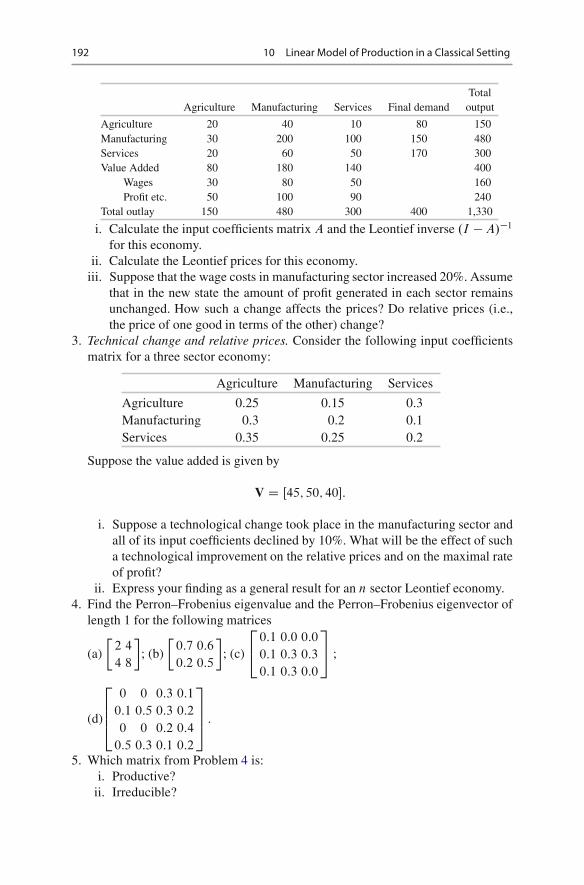
192 10 Linear Model of Production in a Classical Setting
TotalAgriculture Manufacturing Services Final demand output
Agriculture 20 40 10 80 150Manufacturing 30 200 100 150 480Services 20 60 50 170 300Value Added 80 180 140 400
Wages 30 80 50 160Profit etc. 50 100 90 240
Total outlay 150 480 300 400 1,330
i. Calculate the input coefficients matrix A and the Leontief inverse .I �A/�1
for this economy.ii. Calculate the Leontief prices for this economy.
iii. Suppose that the wage costs in manufacturing sector increased 20%. Assumethat in the new state the amount of profit generated in each sector remainsunchanged. How such a change affects the prices? Do relative prices (i.e.,the price of one good in terms of the other) change?
3. Technical change and relative prices. Consider the following input coefficientsmatrix for a three sector economy:
Agriculture Manufacturing Services
Agriculture 0.25 0.15 0.3Manufacturing 0.3 0.2 0.1Services 0.35 0.25 0.2
Suppose the value added is given by
V D Œ45; 50; 40�:
i. Suppose a technological change took place in the manufacturing sector andall of its input coefficients declined by 10%. What will be the effect of sucha technological improvement on the relative prices and on the maximal rateof profit?
ii. Express your finding as a general result for an n sector Leontief economy.4. Find the Perron–Frobenius eigenvalue and the Perron–Frobenius eigenvector of
length 1 for the following matrices
(a)
�2 4
4 8
�; (b)
�0:7 0:6
0:2 0:5
�; (c)
2
40:1 0:0 0:0
0:1 0:3 0:3
0:1 0:3 0:0
3
5 ;
(d)
2
664
0 0 0:3 0:1
0:1 0:5 0:3 0:2
0 0 0:2 0:4
0:5 0:3 0:1 0:2
3
775 :
5. Which matrix from Problem 4 is:i. Productive?
ii. Irreducible?

10.8 Problems 193
6. Consider a three sector economy with the input coefficients matrix
A D2
40:46 0:18 0:25
0:24 0:08 0:46
0:21 0:44 0:19
3
5
and the labor coefficients vector a0 D .0:3; 0:1; 0:2/.Suppose that this economy is analysed in a Sraffian framework.
i. What is the maximum rate of profit for this economy? (Answer: 18.9%)ii. What is the corresponding price vector?
iii. Normalize the price vector by taking sum of prices as equal to one. Using thisnormalization rule find a relation between the rate of profit and the wage ratefor the Sraffa model. Calculate the wage rate when the rate of profit is 10%.
7. Suppose that the input coefficient matrix for a n-sector economy is as follows
A D�
A11 A12
A21 A22
�;
where A11; A12; A21; A22 are matrices of size m �m, n � .n �m/, .n �m/ � n,.n � m/ � .n � m/, respectively. Suppose that A21 D 0, i.e., the first m sectorsdo not use the outputs of the others as inputs. Show that in this economy themaximum growth rate depends exclusively on the production technology of thesesectors and is independent from the production of other sectors.

•

11Linear Programming
The linear programming problem is a general problem of finding the maximal valueof the function f .x/ D .a; x/, where x 2 Rn is a vector of n unknowns and a 2 Rn
is a constant vector, under the restrictions
x � 0 and Ax � d;
where A is a matrix and d is a constant vector. This problem has a lot of applicationsto economic models and practice. Some simple and rather artificial applications arediscussed below.
In mathematical terms the problem is maximizing a linear objective functionunder linear constraints where the relevant variables are restricted to be non-negative. It was first solved by Kantorovich1. In 1947 Dantzig2 made an importantcontribution by introducing a method to solve this kind of problems.
11.1 Diet Problem
Consider a person who has the n-tuple of foods G1; : : : ; Gn in her diet. Eachfood in the diet has m different components (attributes), e.g., fat, protein, calory,sodium, etc.
Let A D ��aij
��
m�nbe a matrix such that aij is the quantity of component i in
one unit of food Gj , for all i D 1; : : : ; m and all j D 1; : : : ; n.
1Leonid Kantorovich (1912–1986) was a Russian mathematician and economist. He developed thelinear programming method in 1939 for a particular industrial problem. In 1975, he shared NobelPrize in Economics for his contributions to the theory of optimal allocation of resources.2George Dantzig (1914–2005) was an American mathematician who made important contributionsin many fields. He developed simplex method which was the first and the most useful effectivemethod to solve linear programming problems.
F. Aleskerov et al., Linear Algebra for Economists, Springer Texts in Businessand Economics, DOI 10.1007/978-3-642-20570-5 11,© Springer-Verlag Berlin Heidelberg 2011
195
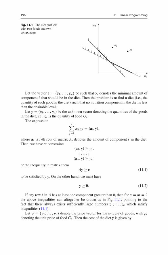
196 11 Linear Programming
Fig. 11.1 The diet problemwith two foods and twocomponents
�
�
��
��
��
��
��
����������������
�1
�2
� y1
� y2
��
�
��
�
��
��
��
��
�������
������
������
������
Let the vector c D .�1; : : : ; �m/ be such that �i denotes the minimal amount ofcomponent i that should be in the diet. Then the problem is to find a diet (i.e., thequantity of each good in the diet) such that no nutrition component in the diet is lessthan the desirable level.
Let y D .�1; : : : ; �n/ be the unknown vector denoting the quantities of the goodsin the diet, i.e., �i is the quantity of food Gi .
The expressionnX
j D1
˛ij �j D .ai ; y/;
where ai is i -th row of matrix A, denotes the amount of component i in the diet.Then, we have m constraints
.a1; y/ � �1;
: : : : : :
.am; y/ � �m;
or the inequality in matrix formAy � c (11.1)
to be satisfied by y. On the other hand, we must have
y � 0: (11.2)
If any row i in A has at least one component greater than 0, then for n D m D 2
the above inequalities can altogether be drawn as in Fig. 11.1, pointing to thefact that there always exists sufficiently large numbers �1; : : : ; �n which satisfyinequalities (11.1).
Let p D .p1; : : : ; pn/ denote the price vector for the n-tuple of goods, with pi
denoting the unit price of food Gi . Then the cost of the diet y is given by

11.2 Linear Production Model 197
.p; y/ DnX
j D1
pj �j : (11.3)
Now, in terms of the matrix A and the vectors c and p, the diet problem is to finda vector y which satisfies (11.1) and (11.2) minimizing at the same time the costfunction (11.3), i.e. 8
<
:
Ay � c;
y � 0;
.p; y/! min :
11.2 Linear Production Model
The linear production model described in Example 1.5 assumed that each economicunit produces only one type of good. Let us consider a slightly different version ofthe same problem.
There are m economic units indexed by i D 1; : : : ; m which produce andconsume n goods indexed by j D 1; : : : ; n.
Let intensities of the units are given by the m-dimensional vector
x D .�1; : : : ; �m/ � 0
where �i denotes the intensity of unit i . Intensities may be measured in several ways,e.g. the total work-hours and the number of employees or the quality of the goodsproduced by an economic unit may be the indicators of its intensity.
We assume that if the intensity of a unit increases by any constant s, then theproduction and the consumption of that unit will also rise by s.
Now, letaj D .˛1j ; ˛2j ; : : : ; ˛mj /;
be a vector such that its i -th component is equal to the quantity of good j consumedor produced by the unit i when it is working with the intensity 1. Define ˛ij to bepositive if good j is produced by unit i , and negative it if is consumed by i . Thenthe matrix
A D ��˛ij
��
n�m
contains the production-consumption data for the economic system.Note that given the intensity vector x, we can uniquely find the quantities of
goods produced and consumed by each unit. Indeed, the sum
�1˛1j C �2˛2j C � � � C �m˛mj D .x; aj /
is equal to the total production (consumption) of good j by the system if it is positive(negative).
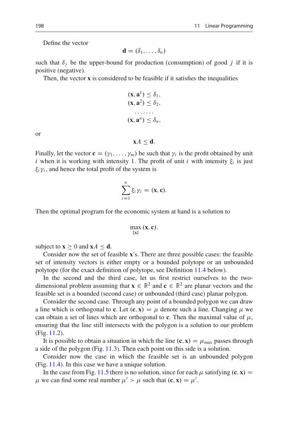
198 11 Linear Programming
Define the vectord D .ı1; : : : ; ın/
such that ıj be the upper-bound for production (consumption) of good j if it ispositive (negative).
Then, the vector x is considered to be feasible if it satisfies the inequalities
.x; a1/ � ı1;
.x; a2/ � ı2;
: : : : : : :
.x; an/ � ın;
orxA � d:
Finally, let the vector c D .�1; : : : ; �m/ be such that �i is the profit obtained by uniti when it is working with intensity 1. The profit of unit i with intensity �i is just�i �i , and hence the total profit of the system is
nX
iD1
�i �i D .x; c/:
Then the optimal program for the economic system at hand is a solution to
maxfxg
.x; c/:
subject to x � 0 and xA � d.Consider now the set of feasible x’s. There are three possible cases: the feasible
set of intensity vectors is either empty or a bounded polytope or an unboundedpolytope (for the exact definition of polytope, see Definition 11.4 below).
In the second and the third case, let us first restrict ourselves to the two-dimensional problem assuming that x 2 R2 and c 2 R2 are planar vectors and thefeasible set is a bounded (second case) or unbounded (third case) planar polygon.
Consider the second case. Through any point of a bounded polygon we can drawa line which is orthogonal to c. Let .c; x/ D � denote such a line. Changing � wecan obtain a set of lines which are orthogonal to c. Then the maximal value of �,ensuring that the line still intersects with the polygon is a solution to our problem(Fig. 11.2).
It is possible to obtain a situation in which the line .c; x/ D �max passes througha side of the polygon (Fig. 11.3). Then each point on this side is a solution.
Consider now the case in which the feasible set is an unbounded polygon(Fig. 11.4). In this case we have a unique solution.
In the case from Fig. 11.5 there is no solution, since for each � satisfying .c; x/ D� we can find some real number �0 > � such that .c; x/ D �0.

11.2 Linear Production Model 199
Fig. 11.2 The case ofbounded feasible set
�
�
����
����
���������
�����
�����
�����
�����
�����
.c; x/ D �max
� x
c
�
Fig. 11.3 An infinitenumber of solutions
�
�
����
����
���������
�����
�����
�����
�����
�����
�����
�����
�����
��
��
��
��
�� .c; x/ D �max
c
����
Fig. 11.4 The uniquesolution
�
�
������������������
����
�����
���
������
����
����
.c; x/ D �max
c
�x
������������
���
Fig. 11.5 No solutions withunbounded feasible set
�
�
������������������
����
�����
�����
����
����
����
c
�
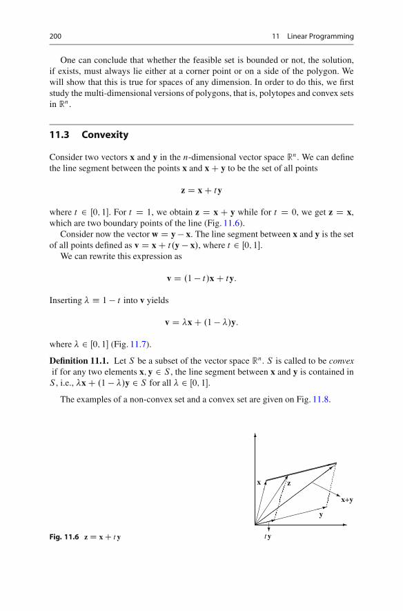
200 11 Linear Programming
One can conclude that whether the feasible set is bounded or not, the solution,if exists, must always lie either at a corner point or on a side of the polygon. Wewill show that this is true for spaces of any dimension. In order to do this, we firststudy the multi-dimensional versions of polygons, that is, polytopes and convex setsin Rn.
11.3 Convexity
Consider two vectors x and y in the n-dimensional vector space Rn. We can definethe line segment between the points x and xC y to be the set of all points
z D xC ty
where t 2 Œ0; 1�. For t D 1, we obtain z D x C y while for t D 0, we get z D x,which are two boundary points of the line (Fig. 11.6).
Consider now the vector w D y� x. The line segment between x and y is the setof all points defined as v D xC t.y � x/, where t 2 Œ0; 1�.
We can rewrite this expression as
v D .1 � t/xC ty:
Inserting � � 1 � t into v yields
v D �xC .1 � �/y:
where � 2 Œ0; 1� (Fig. 11.7).
Definition 11.1. Let S be a subset of the vector space Rn. S is called to be convexif for any two elements x; y 2 S , the line segment between x and y is contained inS , i.e., �xC .1 � �/y 2 S for all � 2 Œ0; 1�.
The examples of a non-convex set and a convex set are given on Fig. 11.8.
�
�
������
���������
�����
������
y
x
x+y
z
ty
��������
��������
��������
��������
����
�Fig. 11.6 z D x C t y

11.3 Convexity 201
Fig. 11.7 v D x C t w
�
�
������
���������
�������
���������
�������
�������
�������
y
x
w
tw
x C tw
�
�
convex set
�
�
non-convexset
Fig. 11.8 Convex and non-convex sets
Theorem 11.1. Let x1; : : : ; xm be any vectors in the vector space Rn. Then the setS of all linear combinations given by
t1x1 C � � � C tmxm
where ti � 0 for all i D 1; : : : ; m andPm
iD1 ti D 1, is convex.
Proof. For any vectors x1; : : : ; xm in Rn, let us define
a D t1x1 C � � � C tmxm
b D s1x1 C � � � C smxm
where ti � 0 , si � 0 ,Pn
iD1 ti D 1 andPn
iD1 si D 1.Consider � D .1 � ˛/aC ˛b for some ˛ 2 Œ0; 1�. We have
� D .1 � ˛/t1x1 C � � � C .1 � ˛/tmxm C ˛s1x1 C � � � C ˛smxm
D Œ.1 � ˛/t1 C ˛s1�x1 C � � � C Œ.1 � ˛/tm C ˛sm�xm
We note that .1 � ˛/ti C ˛si � 0 for all i D 1; : : : ; n since .1 � ˛/ � 0, ti � 0,˛ � 0 and, si � 0. Moreover,
mX
iD1
.1 � ˛/ti C ˛si D .1� ˛/
mX
iD1
ti C ˛
mX
iD1
si D .1 � ˛/C ˛ D 1:
Hence, S is convex. �

202 11 Linear Programming
Theorem 11.2. Let x1; : : : ; xm be any m vectors in R. Any convex set S whichcontains x1; : : : ; xm also contains all linear combinations
t1x1 C � � � C tmxm;
where ti � 0 for all i andPn
iD1 ti D 1.
Proof (by induction). For m D 1, we have t1 D 1 and the statement of the theoremis obviously true. Assume the statement is true for some m � 1 � 1. Take anyx1; : : : ; xm 2 S , and any t1; : : : ; tm satisfying ti � 0 for all i D 1; : : : ; m andPm
iD1 ti D 1. If tm D 1, then the statement is trivially true, because in this caset1 D � � � D tm�1 D 0. Assume now tm ¤ 1. Then we get
�m D t1x1 C � � � C tmxm D .1 � tm/
�t1
1 � tmx1 C � � � C tm�1
1 � tmxm�1
�C tmxm:
Definesi D ti
1 � tm
for all i D 1; : : : ; m � 1. Then the vector
z D s1x1 C � � � C sm�1xm�1;
by induction assumption, lies in S , since si � 0 andPm�1
iD1 si D Pm�1iD1 ti =
.1 � tm/D 1. Thus.1 � tm/zC tmxm D �
is an element of S by the definition of a convex set.The minimal convex set which contains x1; : : : ; xm is called the convex hull of
the set fx1; : : : ; xmg, and is denoted by cofx1; : : : ; xmg. By Theorems 11.1 and 11.2,we get
Corollary 11.3. For any (finite) set x1; : : : ; xm of vectors, its convex hullcofx1; : : : ; xmg consists of all linear combinations given by
t1x1 C � � � C tmxm;
where ti � 0 for all i D 1; : : : ; m andPm
iD1 ti D 1.
Definition 11.2. For any a 2 Rn and ˇ 2 R, the set of points x 2 Rn satisfying
.a; x/ D ˇ;
is called a hyperplane. We denote this hyperplane as H.a; ˇ/Dfx 2 Rnj.a; x/Dˇg.

11.3 Convexity 203
Fig. 11.9 The vector a isorthogonal to the hyperplane
P�
�
������
���������
��
��
��
��
�
��
�� a x1
x2
x2-x1
H.a; ˇ/
Fig. 11.10 The linex C 2y D �4 as ahyperplane H..1; 2/; �4/
�
�
�����������
�������������
�� ��������
x
y
H..1; 2/; �4/
Lemma 11.4. For all ˇ 2 R, any vector a 2 Rn is orthogonal to the hyperplaneH.a; ˇ/ in Rn.
Proof. Take any ˇ 2 R. Then any vector a 2 Rn is orthogonal to the hyperplaneH.a; ˇ/ if and only if it is orthogonal to the vector x2 � x1 which connects twoarbitrary points x1; x2 2 H.a; ˇ/ (Fig. 11.9).
Indeed, .a; x2 � x1/ D .a1; x2/ � .a1; x1/ D ˇ � ˇ D 0, which completes theproof. �
Example 11.1. The line x C 2y D �4 is a hyperplane in R2, and can be rewrittenas H..1; 2/;�4/ (Fig. 11.10).
Lemma 11.5. For all a 2 Rn and ˇ 2 R, the hyperplane H.a; ˇ/ is a convex set.
Proof. Indeed, for any a 2 Rn and ˇ 2 R, consider the hyperplane H.a; ˇ/. Thehyperplane is always non-empty. If Rn D R, then any hyperplane in R is a singleton,and the Lemma is obviously true. For n > 1, take x1; x2 2 H.a; ˇ/. Considerx˛ � .1� ˛/xC ˛x2 for any ˛ 2 Œ0; 1�. Note that
.a; x˛/ D .1 � ˛/.a; x1/C ˛.a; x2/ D .1 � ˛/ˇ C ˛ˇ D ˇ:
Thus, x˛ 2 H.a; ˇ/, and therefore H.a; ˇ/ is convex. �
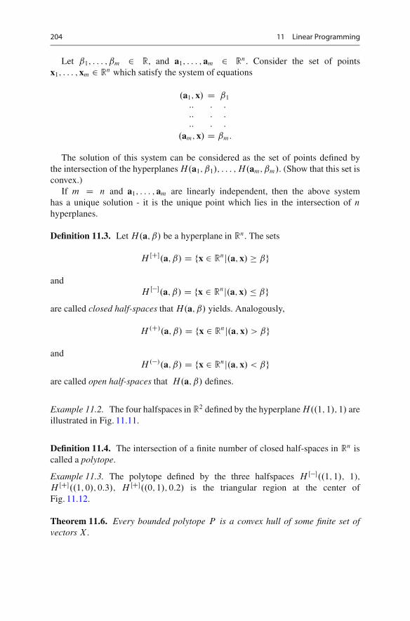
204 11 Linear Programming
Let ˇ1; : : : ; ˇm 2 R, and a1; : : : ; am 2 Rn. Consider the set of pointsx1; : : : ; xm 2 Rn which satisfy the system of equations
.a1; x/ D ˇ1
:: : ::: : ::: : :
.am; x/ D ˇm:
The solution of this system can be considered as the set of points defined bythe intersection of the hyperplanes H.a1; ˇ1/; : : : ; H.am; ˇm/. (Show that this set isconvex.)
If m D n and a1; : : : ; am are linearly independent, then the above systemhas a unique solution - it is the unique point which lies in the intersection of n
hyperplanes.
Definition 11.3. Let H.a; ˇ/ be a hyperplane in Rn. The sets
H ŒC�.a; ˇ/ D fx 2 Rnj.a; x/ � ˇg
andH Œ��.a; ˇ/ D fx 2 Rnj.a; x/ � ˇg
are called closed half-spaces that H.a; ˇ/ yields. Analogously,
H .C/.a; ˇ/ D fx 2 Rnj.a; x/ > ˇg
andH .�/.a; ˇ/ D fx 2 Rnj.a; x/ < ˇg
are called open half-spaces that H.a; ˇ/ defines.
Example 11.2. The four halfspaces in R2 defined by the hyperplane H..1; 1/; 1/ areillustrated in Fig. 11.11.
Definition 11.4. The intersection of a finite number of closed half-spaces in Rn iscalled a polytope.
Example 11.3. The polytope defined by the three halfspaces H Œ��..1; 1/; 1);H ŒC�..1; 0/; 0:3/; H ŒC�..0; 1/; 0:2/ is the triangular region at the center ofFig. 11.12.
Theorem 11.6. Every bounded polytope P is a convex hull of some finite set ofvectors X .
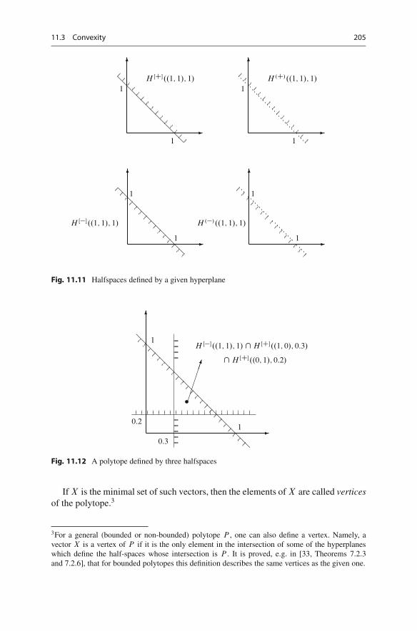
11.3 Convexity 205
�
�
��
��
��
� H ŒC�..1; 1/; 1/
1
1
�
�
H .C/..1; 1/; 1/
1
1
�
�
��
��
��
�
H Œ��..1; 1/; 1/
1
1
�
�
H .�/..1; 1/; 1/
1
1
Fig. 11.11 Halfspaces defined by a given hyperplane
�
�
H Œ��..1; 1/; 1/ \ H ŒC�..1; 0/; 0:3/
\ H ŒC�..0; 1/; 0:2/
1
1
0:3
0:2
��
��
��
��
��
��
�������
Fig. 11.12 A polytope defined by three halfspaces
If X is the minimal set of such vectors, then the elements of X are called verticesof the polytope.3
3For a general (bounded or non-bounded) polytope P , one can also define a vertex. Namely, avector X is a vertex of P if it is the only element in the intersection of some of the hyperplaneswhich define the half-spaces whose intersection is P . It is proved, e.g. in [33, Theorems 7.2.3and 7.2.6], that for bounded polytopes this definition describes the same vertices as the given one.
206 11 Linear Programming
Example 11.4. The polytope defined by 2n hyperplanes H ŒC�.ei; 0/ and H ŒC�.ei; 1/
where i D 1; : : : ; n and ei D .0; : : : ; 1; : : : ; 0/ is the i -th vector of the canonicalbasis, is called a hypercube. It consists of all vectors X D .x1; : : : ; xn/ such that0 � xi � 1 for all i D 1; : : : ; n. Its vertices are 2n vectors of the form .a1; : : : ; an/,where each ai is either 0 or 1.
The next corollary assures the existence of the solution of any linear program-ming problem defined on a bounded polytope.
Corollary 11.7. Let f .x/ D .x; a/ be a linear function of x 2 Rn and let P Dco.v1; : : : ; vk/ be a bounded polytope in Rn. Then the maximal value of f on P isequal to its value on one of the vertices v1; : : : ; vk.
Proof. Let x 2 P . Then x D t1v1 C � � � C tkvk for some ti � 0 such thatt1 C � � � C tk D 1, so that
f .x/ D .x; a/ D .t1v1 C � � � C tkvk; a/ D t1.v1; a/C � � � C tk.vk; a/:
Let .vj ; a/ D maxiD1::k.vi ; a/. Then
f .x/ � .t1 C � � � C tk/.vj ; a/ D .vj ; a/:
Thusmaxx2P
f .x/ D .vj ; a/ D f .vj /:
�
11.4 Transportation Problem
Assume that there are m producer-cities and n consumer-cities of some good, say,potato. Consider the matrix X D �
��ij
��
m�n, where �ij is the quantity of good sent
from producer-city i to consumer-city j (Fig. 11.13).Note that we must have
�ij � 0; i D 1; : : : ; mI j D 1; : : : ; n:
Assume that the production of city i cannot exceed i (due to capacity con-straints), and the consumption of city j must be at least ıi (to survive). In otherwords,
nX
j D1
�ij � i ; i D 1; : : : ; m (11.4)

11.5 Dual Problem 207
��
��
��
����
��
��
��
��
����
��
���
���
�mn
�m2
�m1
�11
�12�1n
�21
�22
�2n
�
�
�
���������������������������
��������������
��
�������������
������������
�
m
2
1
n
2
1
Fig. 11.13 The transportation problem
and
mX
iD1
�ij � ıj ; j D 1; : : : ; n: (11.5)
Let the cost of transporting one unit of good from producer-city i to consumer-cityj is equal to �ij . Then, the optimal transportation program is a solution to
minf�ij g
nX
iD1
nX
j D1
�ij �ij :
subject to (11.4) and (11.5).
11.5 Dual Problem
Let us return to the two-dimensional case of the linear programming problem.Consider a case in which linear programming problem has the unique solution(Fig. 11.14).
Clearly, the point x� in the above figure is a (unique) solution of the problem. Letus rotate the line .c; x/ D �max around x� by an arbitrarily small angle, and obtaina new line .c0; x/ D �0. The new line is not orthogonal to c. So, �0 cannot be themaximum of .c; x/. By the fact that x� uniquely maximizes .c; x/, it follows thatthere exists c0 such that x� maximizes .c0; x/ and .c0; x�/ D �0.
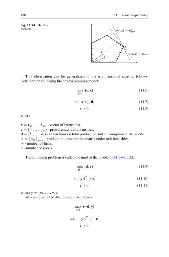
208 11 Linear Programming
Fig. 11.14 The dualproblem
�
�
����
����
���������
�����
�����
�����
�����
�����
.c0; x/ D �0
max
.c; x/ D �max
� x
cc0
�
�����
This observation can be generalized to the n-dimensional case as follows.Consider the following linear programming model:
maxfxg
.c; x/ (11.6)
s.t. xA � d; (11.7)
x � 0; (11.8)
where
x D .�1; : : : ; �m/ - vector of intensities,c D .�1; : : : ; �m/ - profits under unit intensities,d D .ı1; : : : ; ın/ - restrictions on total production and consumption of the goods,A D ��˛ij
��m�n
- production-consumption matrix under unit intensities,m - number of firms,n - number of goods.
The following problem is called the dual of the problem (11.6)–(11.8):
minfyg
.d; y/ (11.9)
s.t. yAT � c; (11.10)
y � 0; (11.11)
where y D .�1; : : : ; �n/.We can rewrite the dual problem as follows:
maxfyg
.�d; y/
s.t. � yAT � �c;
y � 0;
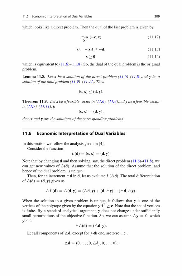
11.6 Economic Interpretation of Dual Variables 209
which looks like a direct problem. Then the dual of the last problem is given by
minfxg
.�c; x/ (11.12)
s.t. � xA � �d; (11.13)
x � 0; (11.14)
which is equivalent to (11.6)–(11.8). So, the dual of the dual problem is the originalproblem.
Lemma 11.8. Let x be a solution of the direct problem (11.6)–(11.8) and y be asolution of the dual problem (11.9)–(11.11). Then
.c; x/ � .d; y/:
Theorem 11.9. Let x be a feasible vector in (11.6)–(11.8) and y be a feasible vectorin (11.9)–(11.11). If
.c; x/ D .d; y/;
then x and y are the solutions of the corresponding problems.
11.6 Economic Interpretation of Dual Variables
In this section we follow the analysis given in [4].Consider the function
L.d/ D .c; x/ D .d; y/:
Note that by changing d and then solving, say, the direct problem (11.6)–(11.8), wecan get new values of L.d/. Assume that the solution of the direct problem, andhence of the dual problem, is unique.
Then, for an increment4d in d, let us evaluate L.4d/. The total differentiationof L.d/ D .d; y/ gives us
4L.d/ D 4.d; y/ D .4d; y/C .d;4y/C .4d;4y/:
When the solution to a given problem is unique, it follows that y is one of thevertices of the polytope given by the equation yAT � c. Note that the set of verticesis finite. By a standard analytical argument, y does not change under sufficientlysmall perturbations of the objective function. So, we can assume 4y D 0, whichyields
4L.d/ D .4d; y/:
Let all components of4d, except for j -th one, are zero, i.e.,
4d D .0; : : : ; 0;4ıj ; 0; : : : ; 0/:

210 11 Linear Programming
Then we can write4L.d/ D 4ıj �j :
For the profit maximization problem,4L.d/ is measured in monetary terms, say, indollars, while 4ıj is measured in units of production-consumption goods. So, �j
must be in dollars, and can be interpreted as the unit price of the goods.Inequality (11.10) can be explicitly written as
nX
j D1
˛ij �j � �i ; .i D 1; : : : ; m/ (11.15)
for the optimal solution y. Since for all j , �j being a price is always nonnegative, theleft hand side of (11.15) may have both positive and negative components. Recallthat positive (negative) ˛ij ’s correspond to production (consumption). So, the sumof positive components in the left hand side of (11.15) denote the revenues that uniti obtains by selling goods when it works with intensity one. Analogously, the sum ofnegative components in the left hand side of (11.15) denote the (minus) expendituresfor purchasing goods incurred by the unit i when working with intensity one. Thus,for each unit (11.15) can be written as
revenues� expenditures � total profits, (11.16)
when the economic units work with the intensity 1. If, for some unit, (11.16) holdswith a strict inequality, we say that this unit is not fully utilizing its resources. Inthat case, we claim that the intensity of this unit in the optimal solution must be 0.
Theorem 11.10 (Equilibrium Theorem). Let x and y are feasible vectors for thedirect and dual problems, respectively, which are described above. Then thesevectors are solutions to the corresponding problems if and only if for all i D1; : : : ; m and j D 1; : : : ; n
�j D 0 ifmX
iD1
˛ij �i � ıj (11.17)
and
�i D 0 ifnX
j D1
˛ij �j � �i : (11.18)
Remark 11.1. Note that (11.18) validates our previous claim that if a unit is notefficiently operating, then it does not take part in the optimal program. On theother hand, from (11.17) we observe that if some resource is not fully utilized inthe optimal program, then its price equals zero. A natural question that follows iswhether it has been ever the case that a resource had a zero price. As it is emphasizedin [4], the answer is yes! In the ‘old days’ demand for water was much below of its(natural) supply, and thus factories did not pay for it.

11.7 A Generalization of the Leontief Model 211
11.7 A Generalization of the Leontief Model: MultipleProduction Techniques and Linear Programming
In Leontief model (Sect. 10.2) each production technique is assumed to be produc-ing only one commodity (no joint production assumption) and each commodity isproduced only by one production technique (no alternative production techniques).In this section, the second assumption will be relaxed to allow the model to dealwith the problem of choice of techniques. The remaining assumptions of the modelwill be retained.
Suppose there are again m commodities, each can be produced by n.i/ differenttechniques .i D 1; : : : ; m/. Let
X
i2I
n.i/ D n; n.i/ � 1; I D f1; : : : ; mg
Let us defineQA D . Qaij /m�n (11.19)
as the technology matrix that represent the available production techniques, wherem < n. The problem then is to identify a submatrix of QA that serves best for thepolicy maker’s purpose. The solution of this problem requires a clear definition ofthe purpose of the decision maker and the appropriate mathematical apparatus tosolve it. Consider the following example.
Example 11.5. Consider an economy that can be characterized by the followingconditions:1. There are m commodities and n.> m/ techniques of production.
Let xi denote the activity level of production technique i . If it is foundmeaningful to operate this activity then xj > 0, if not xj D 0.
2. The technology matrix is given by (11.19).3. All commodities are treated as resources. At the beginning of the production
period t , the initial endowment of resources is given by the m-dimensionalcolumn vector
! D
2
664
!1
!2
� � �!m
3
775
each component of this vector gives the amount of commodity i .I D 1; : : : ; m/
available to be used for production.4. Let
vT D .1; : : : ; n/
be the row vector of value added coefficients (value added created by the processwhen one unit of output is produced).

212 11 Linear Programming
5. Suppose the policymaker’s problem is to maximize the total value added at time t,under the conditions stated above.Then this problem can be expressed as
max vT x
subject toQA x � !;
and since activity level is non-negative, the solution should also satisfy the followingset of conditions
x � 0:
We see that this is a linear programming problem.
11.8 Problems
1. Show that Rn is a convex set.2. Show that the intersection of any two convex sets in Rn is convex.3. Let A W Rn ! Rn is a linear operator, and let X be a set of all vectors x 2 Rn
such thatA.x/ � 0:
Show that X is convex.4. Let a 2 Rn and ˛ 2 R. Show that the sets
fx 2 Rnj.a; x/ � ˛g and fx 2 Rnj.a; x/ � ˛g
are convex.5. Let X D fxg where x 2 Rn. Show that X is convex.6. Draw the convex hull of the following sets of points:
(a) .�2; 0/; .0;�2/; .0; 0/; .0; 2/; .1; 0:5/; .2; 0/.
(b) .2; 2/; .�2; 2/; .0; 0/; .0; 1/; .0; 2/; .�2;�2/; .2;�2/; .1;�1/.7. Determine whether the following sets are convex:
(a) X D f.x1; x2/ j x21 C x2
2 � 1g(b) X D f.x1; x2/ j x1; x2 � 1; x1 � 0; x2 � 0g(c) X D f.x1; x2/ j x2
1 C 2x22 � 4g
8. Consider the hyperplane
H D f.x1; x2; x3; x4; x5/ 2 R5 j x1 � x2 C 4x3 � 2x4 C 6x5 D 1g:

11.8 Problems 213
In which half space does each of the following points lie?a. .1; 1; 1; 1; 1/
b. .2; 7;�1; 0;�3/
c. .0; 1; 1; 4; 1/
9. Let .a; x/ D 0 be a hyperplane in Rn. Prove that it is a subspace of Rn.10. Determine whether the union of any m convex sets X1; : : : ; Xm in Rn is convex.11. Mr Holst has 100 acres (404,686 square meters) of land where he can plant
wheat and/or barley. His problem is to maximize his expected net revenue. Hiscapital is $1,000. It costs $7 to plant a acre of wheat and $5 to plant a acre ofbarley. Mr Holst is able to secure 150 of days of labor per season. Wheat andbarley require, respectively, 2 and 3 days of labor per acre.
According to the existing information, revenue from an acre of wheat andbarley are $75 and $55, respectively.
How many acres of each cereal should be planted to maximize Mr Holst’snet revenue?
12. Suppose that a fund manager is entrusted with $1 million to be invested insecurities. The feasible alternatives are government bonds, automotive andtextile companies. The list of alternatives and the expected returns are givenbelow
Expected return (%)Government bonds 3.5Auto producer A 5.5Auto producer B 6.5
Textile company C 6Textile company D 9
The following investment guidelines were imposed:(a) Neither industry (auto or textile) should receive more than 50% of the
amount to be invested.(b) Government bonds should be at least 35% of the auto industry investments.(c) The investment in high yield, high risk Textile Company D can not be more
than 65% of the total textile industry investments.Find the composition of the portfolio that maximizes the projected return, underthe conditions given above.
13. A research institute has an endowment fund of $10 million. The researchinstitute, naturally, concerned with the risk it is taking. On the other hand it alsoneeds to generate $400,000 to cover its expenses. The institute has two options:Investing in low risk money market fund (x) or to high risk stock funds (y).
Money market fund’s risk scale is 4, whereas the stock funds’ is 9. Thereturn of these funds, on the other hand, is as follows: Money market fund 4%and stock fund 10%. The price of a money market fund certificate is $50 andthe price of a stock fund certificate is $150.

214 11 Linear Programming
The management of the institute decided that, for liquidity purposes, theamount invested in money markets should not be less than $90,000.
Using this information determine the optimal portfolio allocation for theresearch institute.
14. Consider a simple two sector economy, where labor is the sole productionfactor. The input coefficients matrix for this economy is given as
A D�
0:1 0:2
0:3 0:15
�;
which implies that both goods are used in production of itself and the other one.The labor coefficients vector is given by
a0 D .0:05; 0:07/:
The total labor supply is 150 (million man-hours).In the previous year the final consumption of first sector output C1 was
$1,000 (million), and the second sector output C2 was $440 (million).Suppose that the social welfare is a linear function of consumption and given by
W.C1; C2/ D C1 C .1; 1/C2:
Suppose the government wants to maximize social welfare without reducingthe consumption of each good below their previous levels. What will be theoptimal solution?
15. Motivation. The following problem is a simple exercise in the two-gap growththeory. This theory dates back to early 1960s and approaches the developmentproblem by observing the fact that developing countries need both savings toinvest and foreign exchange to import the necessary goods. Therefore they facetwo problems: the first is the saving constraint and the second is the foreignexchange constraint. Therefore for such countries using simple Harrod-Domartype of framework, which takes into account only the savings constraint, maynot be sufficient.Question. Suppose the economy at hand is described by the following set ofstructural equations:1. Aggregate Demand.
Y d D C C I CX �M;
whereY d : Aggregate Demand (GDP measured from demand side).C : Consumption.I : Investment.X : Exports.M : Imports.

11.8 Problems 215
2. Capacity Growth.The increase in the production capacity of the economy depends on the
amount of investment. It is assumed that marginal capital output ratio, i.e.,I=�Y D 4; this means that one unit of investment produces 0.25 units ofGDP. This relation can be expressed as
�Y D Y s � Y s�1 D 0:25I;
where Y s and Y s�1 are capacity aggregate output levels of present and theprevious periods. Suppose that
Y s�1 D 300:
Therefore the above equation can be written as
Y s D 0:25I C 300:
3. Saving and Investment.Investments are either financed by domestic savings (S ) or external
borrowing (F ):I D S C F:
Suppose that the domestic savings is a linear function of the GDP (Y ),
S D 0:2Y;
and foreign borrowing is forecasted to be at most 20, i.e.,
F � 20:
Therefore,I � 0:2Y C 20:
4. Equilibrium Condition.The economy is in equilibrium when aggregate supply (Y s) is equal to
aggregate demand (Y d ). Equilibrium output level is denoted by Y :
Y D Y s D Y d :
5. Import Equation.The 5% of the total consumption and 15% of the investment goods are
imported. Therefore,M D 0:05C C 0:15I:

216 11 Linear Programming
6. Foreign Exchange Constraint.The country can get access to foreign exchange either by exports or
through borrowing from abroad. In other words, imports can not exceed thesum total of them, i.e.,
M � X C F:
For the sake of simplicity lets assume that the maximum amount ofexports for the current year is estimated to be 100, that is,
X � 100:
Therefore, the foreign exchange constraint can be written as
M � 100C 20 D 120:
The government wants to maximize current GDP, under saving andforeign exchange constraints. However, the government also does not wantthe current consumption level to be lower than the one of the previous period.
How much investment is needed? What is the new GDP level? Will therebe an increase in total consumption?

ANatural Numbers and Induction
In this appendix, we discuss one powerful and general method to deduce theoremsand formulas depending on a natural parameter. This method, called induction,could be illustrated by the domino effect: if dominoes are stood on end one slightlybehind the other, a slight push on the first will topple the others one by one.
As a toy example, let us prove that the area of the rectangle of the size 5 � n isequal to 5n. For n D 1, the rectangle can obviously be cut up into 5 unit squares, soits area is equal to 5 (the first domino falls down). Now, for n D 2 we explore thedomino effect and cut up the rectangle into two ones of size 5 � 1. This gives thearea 5C 5 D 5 � 2. For n D 3, we cut up the rectangle into the rectangles 5 � 2 and5 � 1: this gives the area 5 � 2C 5 � 1 D 5 � 3. By the same way, we cut up any largerectangle of the size 5 � n into two ones, that is, the rectangle 5 � .n � 1/ and the‘ribbon’ 5 � 1 (see Fig. A.1). At some moment, we can assume that the area of thefirst one is known to be Sn�1 D 5 � .n� 1/ (the .n� 1/-th domino has fallen down),so, we calculate the area as Sn D 5 � .n � 1/C 5 � 1 D 5 � n.
Similar (and slightly more complicated) methods can be applied in manyproblems. In order to give their formal description, we first discuss a formalintroduction to natural numbers.
A.1 Natural Numbers: Axiomatic Definition
Natural numbers are known as the main and the basic objects in mathematics. Manycomplicated things such as rational and real numbers, vectors, and matrices can bedefined via the natural numbers. “God made the integers; all else is the work ofman”, said Leopold Kronecker, one of the most significant algebraists of nineteenthcentury.
What are the natural numbers? This question admits a lot of answers, all indifferent levels of abstraction. The naıve definition says that these are just thenumbers used in counting, that is, 0; 1; 2; : : : In the geometry of the real line, the
F. Aleskerov et al., Linear Algebra for Economists, Springer Texts in Businessand Economics, DOI 10.1007/978-3-642-20570-5,© Springer-Verlag Berlin Heidelberg 2011
217

218 A Natural Numbers and Induction
Sn-1
n-1
Fig. A.1 The area of a rectangle: proof by induction
set of natural numbers N is defined as the set of the following points in the line:an initial point (say, O); the right-hand end of the unit segment whose left-handend is O ; the right-hand end of the unit segment whose left-hand end is the justdefined point; and so on. In the set theory, every natural number n is considered asthe simplest set of n elements: 0 D ;; 1 D f0g; 2 D f0; 1g; 3 D f0; 1; 2g etc. Theseset-theoretical numbers play the role of etalons for counting all other finite sets.
Let us give the most general definition, that covers all previous ones. It is basedon the axioms due to Peano1 (1889). Assume the N is a set, 0 is an element of theset N , and s W N ! N is a function (called ‘successor’). The set N is called a setof natural numbers, if the following three Peano axioms are satisfied.1. If s.m/ D s.n/, then m D n. (This means that the function s is injective).2. There is no such n that s.n/ D 0.3. (Induction axiom). Suppose that there is a subset A � N such that (1) 0 2 A and
(2) for every n 2 A we have s.n/ 2 A. Then A D N .For example, one can define an operation n 7! nC 1 as nC 1 WD s.n/.
Exercise A.1. Define an operation s for the above versions of natural numbers,that is, for the collection N1 of points in a real line and for the sequence of sets:0 D ;; 1 D f0g; 2 D f0; 1g : : :
Let us define also an operation n 7! n C m via the two rules: n C 0 WD n andnC .mC 1/ WD s.nC m/. Let A be the set of the numbers m 2 N for which wecan calculate the sum nC m using this rule. Then 0 2 A (by the first rule) and forevery m 2 A we have mC 1 2 A (by the second rule). It follows from the inductionaxiom that the sum nCm is defined for all m; n 2 N .
1Giuseppe Peano (1858–1932) was a famous Italian mathematician. Being one of the founders ofmathematical logic and set theory, he was also an author of many analytical discoveries includinga continuous mapping of a line onto every point of a square. Another his discovery was Latino sineFlexione (or Interlingua), an artificial language based on Latin with simpler grammar.

A.2 Induction Principle 219
Exercise A.2. Give definitions (in a similar way as the above definition of theaddition) of the following operations with natural number m and n:1. m � n.2. mn.
This way to define an operation (from each natural number m to the nextnumber m C 1 an so on) is called recursion. For example, a recursive formulagives a definition of the determinant of a matrix of order n, see the formula (3.6).The recursion definitions are appropriate for using in the induction reasonings, asdescribed below.
A.2 Induction Principle
In order to deduce any significant property of natural numbers from the aboveaxioms, one should use a special kind of reasoning, called the induction principle,or mathematical induction.
Let P.n/ be an arbitrary statement concerning a natural number n (like, forexample, “n is equal to 5”, or nC 2 D 2C n, or “either n � 2 or xn C yn ¤ zn forany natural x; y; z”).
Theorem A.1. Let P.n/ be a statement2 depending on element n of a set of naturalnumbers N . Suppose that the following two assumptions hold:1. (The basis, or The initial step) P.0/ is true.2. (The inductive step) P.nC 1/ is true provided that P.n/ is true.
Then P.n/ is true for every n 2 N .
Note that the element n here is called induction variable, and the assumption thatP.n/ holds in the inductive step is called induction assumption.
Proof. Let A be a set consisting of all natural numbers n 2 N such that P.n/ istrue. According to the basis of induction, we have 0 2 A. By the induction step, forevery n 2 A we have also nC 1 2 A. Thus, we can apply the induction axiom andconclude that A D N . �Example A.1. Let us prove the formula
0C 1C 2C � � � C n D n.nC 1/
2: (A.1)
Let P.n/ be the above equality. For n D 0 it is obviously true: 0 D 0�12
. Thisgives the basis of the induction. To prove the induction step, let us assume that thestatement P.n/ is true for some n, that is, the equality (A.1) holds. We have to
2Note that we do not give here a strong mathematical definition of a term ‘statement’. At least, allstatements consisting of arithmetical formulas with additions like “for every natural n” or “thereexists natural x such that” are admissible.
220 A Natural Numbers and Induction
deduce the statement P.nC 1/, that is, the same formula with n replaced by nC 1.Using the statement P.n/, we re-write the left hand side of the equality P.n C 1/
as follows:
0C 1C 2C � � � C nC .nC 1/ D n.nC 1/
2C .nC 1/ D .nC 1/.nC 2/
2:
This equality is equivalent to P.n C 1/, so, the induction step is complete. By theinduction principle, we conclude that P.n/ holds for all n.
Example A.2. In this example we deduce some standard properties of naturalnumbers from Peano axioms.
First, let us consider the following statement P.n/: 0 C n D n. By the abovedefinition of addition, we have mC 0 D m for all m 2 N , hence 0C 0 D 0. Thisgives the basis of the induction: P.0/ is true. To prove the induction step, let usassume that the statement P.n/ is true for some n, that is, 0Cn D n. Using this factand the definition of addition, we obtain: 0C .nC 1/ D s.0C n/ D s.n/ D nC 1,i.e., we have deduced the statement P.nC 1/. Since both the basis of the inductionand the inductive step are true, we conclude that P.n/ is true for all n.
Now, let us prove the associativity property
.l Cm/C n D l C .mC n/
for all natural l; m; n (we denote this statement by Sl;m.n/). Again, let us apply theinduction (on the number n). For n D 0, we get the trivial statement Sl;m.0/ W l Cm D l Cm, which is obviously true, so, the basis of the induction Sm.0/ is proved.To show the induction step, it remains to show that Sl;m.n C 1/ is true for all l; m
provided that Sl;m.n/ is. Using the equalities Sl;m.n/, we have .l Cm/C .nC 1/ Ds..l Cm/Cn/ D s.l C .mCn// D lC s.mCn/ D l C .mC .nC 1//. This givesSl;m.nC 1/. Hence, the proof is complete.
Now, let us prove the following statement Qm.n/
mC .nC 1/ D .mC 1/C n:
We proceed by the induction on the variable n. For n D 0, we have mC1 D mC1:this is the basis Qm.0/ of the induction. To show the induction step, let us assumethat for some n the statement Qm.n/ is true for all m. We have to show Qm.nC 1/.Using the assumption, we have
mC .nC 2/ D s.mC .nC 1// D s..mC 1/C n/ D .mC 1/C .nC 1/:
So, we have deduced Qm.n C 1/. By the induction principle, the equality Qm.n/
holds for all m and n.
A.2 Induction Principle 221
Finally, let us show the commutativity property
mC n D nCm
for all m; n 2 N . We proceed by the induction on n. For n D 0 we get the abovestatement P.m/, hence the initial step holds. To prove the induction step, we use theinduction assumption (the equality mC n D nCm) and the statement Qn.m/:
mC .nC 1/ D s.mC n/ D s.nCm/ D nC .mC 1/ D .nC 1/Cm:
Thus, the induction step is proved, and the induction is complete. �Exercise A.3. Using the definition of multiplication of natural numbers given inExercise A.2, prove the following standard properties:1. a.bc/ D .ab/c.2. ab D ba.
The following version of Theorem A.1 is called a weak induction principle.
Corollary A.2. Let P.n/ be a statement depending on element n of a set of naturalnumbers N . Suppose that the following two assumption hold:1. P.n0/ is true for some n0 2 N .2. P.nC 1/ is true provided that P.n/ is true, where n � n0.
Then P.n/ is true for every n � n0.
Proof. Let P 0.n/ be the following statement: ‘P.n0 C n/ is true’. Then the aboveconditions on P.n/ are equivalent to the conditions of Theorem A.1 for thestatement P 0.n/. Hence, we apply the induction principle and deduce that P 0.n/
is true for all n. This means that P.n/ is true for all n � n0. �
Example A.3. Let us solve the inequality
2n > 3n; (A.2)
where n > 0 is an integer.It is easy to check that the inequality fails for 0 < n � 3, while for n D 4 it
holds: 24 > 3 � 4. It is natural to assume that the inequality holds for all n � 4. Howto prove the assumption?
Let us apply the weak induction principle with n0 D 4. The statement P.n/ isthen the inequality (A.2). The initial step P.4/ is done. To prove the induction step,we try to deduce P.n C 1/ from P.n/, where n � 4. Consider the left hand side2nC1 of P.nC 1/. According to P.n/, we have
2nC1 D 2 � 2n > 2 � 3n D 6n:
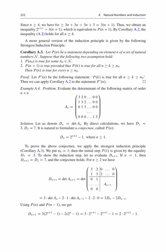
222 A Natural Numbers and Induction
Since n � 4, we have 6n � 3n C 3n > 3nC 3 D 3.nC 1/. Thus, we obtain aninequality 2nC1 > 3.nC 1/, which is equivalent to P.nC 1/. By Corollary A.2, theinequality (A.2) holds for all n � 4.
A more general version of the induction principle is given by the followingStrongest Induction Principle.
Corollary A.3. Let P.n/ be a statement depending on element n of a set of naturalnumbers N . Suppose that the following two assumption hold:1. P.n0/ is true for some n0 2 N .2. P.nC 1/ is true provided that P.k/ is true for all n � k � n0.
Then P.n/ is true for every n � n0.
Proof. Let P 0.n/ be the following statement: ‘P.k/ is true for all n � k � n0’.Then we can apply Corollary A.2 to the statement P 0.n/. �
Example A.4. Problem. Evaluate the determinant of the following matrix of ordern � n
An D
0
BBBBB@
3 2 0 : : : 0 0
1 3 2 : : : 0 0
0 1 3 : : : 0 0
: : :
0 0 0 : : : 1 3
1
CCCCCA
Solution. Let us denote Dn D det An. By direct calculations, we have D1 D3; D2 D 7. It is natural to formulate a conjecture, called P.n/:
Dn D 2nC1 � 1; where n � 1:
To prove the above conjecture, we apply the strongest induction principle(Corollary A.3). We put n0 D 1: then the initial step P.1/ is given by the equalityD1 D 3. To show the induction step, let us evaluate DnC1. If n D 1, thenDnC1 D D2 D 7, and the conjecture holds. For n � 2 we have
DnC1 D det AnC1 D det
0
BBBBB@
3 2 0 : : : 0
1 3 2 : : : 0
0 1
: : : : : : An�1
0 0
1
CCCCCA
D 3 � det An � 2 � 1 � det An�1 � 2 � 2 � 0 D 3Dn � 2Dn�1:
Using P.n/ and P.n � 1/, we get
DnC1 D 3.2nC1 � 1/� 2.2n � 1/ D 3 � 2nC1 � 2nC1 � 1 D 2 � 2nC2 � 1:
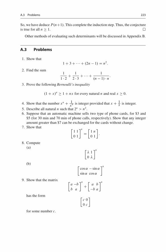
A.3 Problems 223
So, we have deduce P.nC1/. This complete the induction step. Thus, the conjectureis true for all n � 1. �
Other methods of evaluating such determinants will be discussed in Appendix B.
A.3 Problems
1. Show that1C 3C � � � C .2n � 1/ D n2:
2. Find the sum1
1 � 2 C1
2 � 3 C � � � C1
.n � 1/ � n:
3. Prove the following Bernoulli’s inequality
.1C x/n � 1C nx for every natural n and real x � 0:
4. Show that the number xn C 1xn is integer provided that x C 1
x is integer.
5. Describe all natural n such that 2n > n2.6. Suppose that an automatic machine sells two type of phone cards, for $3 and
$5 (for 30 min and 70 min of phone calls, respectively). Show that any integeramount greater than $7 can be exchanged for the cards without change.
7. Show that �1 1
0 1
�n
D�
1 n
0 1
�:
8. Compute(a) �
� 1
0 �
�n
(b) �cos ˛ � sin ˛
sin ˛ cos ˛
�n
9. Show that the matrix �a �b
b a
�n
C�
a b
�b a
�n
has the form �c 0
0 c
�
for some number c.

224 A Natural Numbers and Induction
10. Show that the determinant of order n
ˇˇˇˇˇˇˇˇˇ
0 1 0 : : : 0 0
�1 0 1 : : : 0 0
0 �1 0 : : : 0 0:::
::::::
: : ::::
:::
0 0 0 : : : �1 0
ˇˇˇˇˇˇˇˇˇ
is equal to .1C .�1/n/=2.
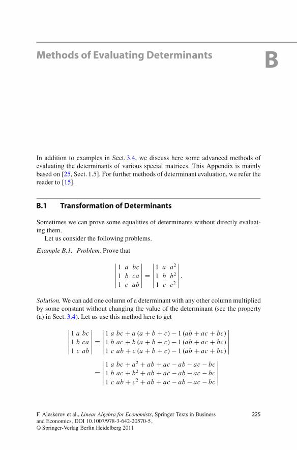
BMethods of Evaluating Determinants
In addition to examples in Sect. 3.4, we discuss here some advanced methods ofevaluating the determinants of various special matrices. This Appendix is mainlybased on [25, Sect. 1.5]. For further methods of determinant evaluation, we refer thereader to [15].
B.1 Transformation of Determinants
Sometimes we can prove some equalities of determinants without directly evaluat-ing them.
Let us consider the following problems.
Example B.1. Problem. Prove that
ˇˇˇˇˇ
1 a bc
1 b ca
1 c ab
ˇˇˇˇˇDˇˇˇˇˇ
1 a a2
1 b b2
1 c c2
ˇˇˇˇˇ:
Solution. We can add one column of a determinant with any other column multipliedby some constant without changing the value of the determinant (see the property(a) in Sect. 3.4). Let us use this method here to get
ˇˇˇˇˇ
1 a bc
1 b ca
1 c ab
ˇˇˇˇˇDˇˇˇˇˇ
1 a bc C a .aC b C c/ � 1 .ab C ac C bc/
1 b ac C b .aC b C c/ � 1 .ab C ac C bc/
1 c ab C c .aC b C c/ � 1 .ab C ac C bc/
ˇˇˇˇˇ
Dˇˇˇˇˇ
1 a bc C a2 C ab C ac � ab � ac � bc
1 b ac C b2 C ab C ac � ab � ac � bc
1 c ab C c2 C ab C ac � ab � ac � bc
ˇˇˇˇˇ
F. Aleskerov et al., Linear Algebra for Economists, Springer Texts in Businessand Economics, DOI 10.1007/978-3-642-20570-5,© Springer-Verlag Berlin Heidelberg 2011
225
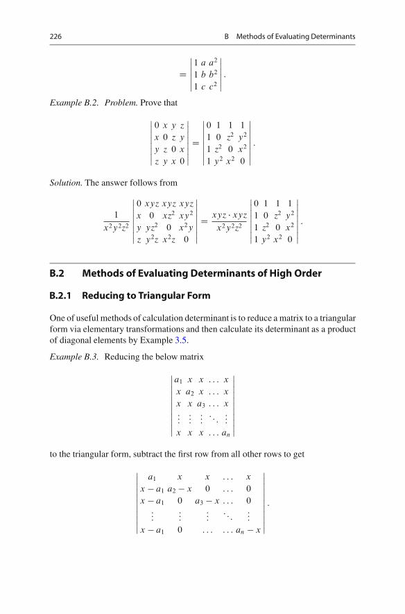
226 B Methods of Evaluating Determinants
Dˇˇˇˇˇ
1 a a2
1 b b2
1 c c2
ˇˇˇˇˇ:
Example B.2. Problem. Prove that
ˇˇˇˇˇˇˇ
0 x y zx 0 z y
y z 0 x
z y x 0
ˇˇˇˇˇˇˇ
D
ˇˇˇˇˇˇˇ
0 1 1 1
1 0 z2 y2
1 z2 0 x2
1 y2 x2 0
ˇˇˇˇˇˇˇ
:
Solution. The answer follows from
1
x2y2z2
ˇˇˇˇˇˇ
0 xyz xyz xyzx 0 xz2 xy2
y yz2 0 x2y
z y2z x2z 0
ˇˇˇˇˇˇ
D xyz � xyz
x2y2z2
ˇˇˇˇˇˇ
0 1 1 1
1 0 z2 y2
1 z2 0 x2
1 y2 x2 0
ˇˇˇˇˇˇ
:
B.2 Methods of Evaluating Determinants of High Order
B.2.1 Reducing to Triangular Form
One of useful methods of calculation determinant is to reduce a matrix to a triangularform via elementary transformations and then calculate its determinant as a productof diagonal elements by Example 3.5.
Example B.3. Reducing the below matrix
ˇˇˇˇˇˇˇˇˇ
a1 x x : : : x
x a2 x : : : x
x x a3 : : : x:::
::::::
: : ::::
x x x : : : an
ˇˇˇˇˇˇˇˇˇ
to the triangular form, subtract the first row from all other rows to get
ˇˇˇˇˇˇˇˇˇ
a1 x x : : : x
x � a1 a2 � x 0 : : : 0
x � a1 0 a3 � x : : : 0:::
::::::
: : ::::
x � a1 0 : : : : : : an � x
ˇˇˇˇˇˇˇˇˇ
:
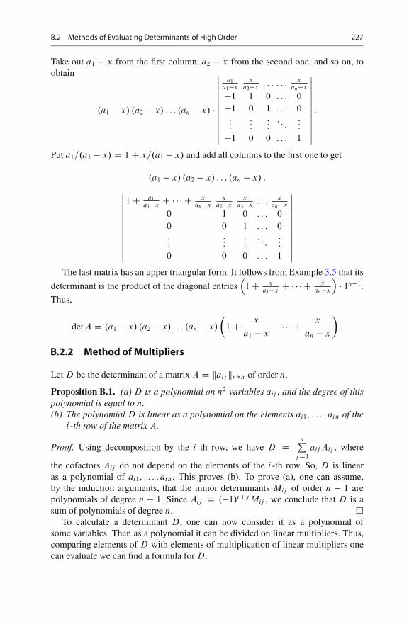
B.2 Methods of Evaluating Determinants of High Order 227
Take out a1 � x from the first column, a2 � x from the second one, and so on, toobtain
.a1 � x/ .a2 � x/ : : : .an � x/ �
ˇˇˇˇˇˇˇˇˇˇ
a1
a1�xx
a2�x: : : : : : x
an�x
�1 1 0 : : : 0
�1 0 1 : : : 0:::
::::::
: : ::::
�1 0 0 : : : 1
ˇˇˇˇˇˇˇˇˇˇ
:
Put a1=.a1 � x/ D 1C x=.a1 � x/ and add all columns to the first one to get
.a1 � x/ .a2 � x/ : : : .an � x/ :
ˇˇˇˇˇˇˇˇˇˇ
1C a1
a1�xC � � � C x
an�xx
a2�xx
a3�x: : : x
an�x
0 1 0 : : : 0
0 0 1 : : : 0:::
::::::
: : ::::
0 0 0 : : : 1
ˇˇˇˇˇˇˇˇˇˇ
The last matrix has an upper triangular form. It follows from Example 3.5 that its
determinant is the product of the diagonal entries�1C x
a1�xC � � � C x
an�x
�� 1n�1.
Thus,
det A D .a1 � x/ .a2 � x/ : : : .an � x/
�1C x
a1 � xC � � � C x
an � x
�:
B.2.2 Method of Multipliers
Let D be the determinant of a matrix A D kaij kn�n of order n.
Proposition B.1. (a) D is a polynomial on n2 variables aij , and the degree of thispolynomial is equal to n.(b) The polynomial D is linear as a polynomial on the elements ai1; : : : ; ain of the
i -th row of the matrix A.
Proof. Using decomposition by the i -th row, we have D DnP
j D1
aij Aij , where
the cofactors Aij do not depend on the elements of the i -th row. So, D is linearas a polynomial of ai1; : : : ; ain. This proves (b). To prove (a), one can assume,by the induction arguments, that the minor determinants Mij of order n � 1 arepolynomials of degree n � 1. Since Aij D .�1/iCj Mij , we conclude that D is asum of polynomials of degree n. �
To calculate a determinant D, one can now consider it as a polynomial ofsome variables. Then as a polynomial it can be divided on linear multipliers. Thus,comparing elements of D with elements of multiplication of linear multipliers onecan evaluate we can find a formula for D.
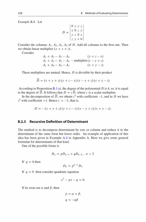
228 B Methods of Evaluating Determinants
Example B.4. Let
D D
ˇˇˇˇˇˇ
0 x y zx 0 z y
y z 0 x
z y x 0
ˇˇˇˇˇˇ
Consider the columns A1; A2; A3; A4 of D. Add all columns to the first one. Thenwe obtain linear multiplier .x C y C z/.
ConsiderA1 C A2 � A3 �A4
A1 C A3 � A2 �A4
A1 C A4 � A2 �A3
�multiplier.y C z � x/
.x � y C z/
.x C y � z/
These multipliers are mutual. Hence, D is divisible by their product
eD D .x C y C z/ .y C z � x/ .x � y C z/ .x C y � z/
According to Proposition B.1 a), the degree of the polynomial D is 4, so, it is equalto the degree of eD. It follows that D D ceD, where c is a scalar multiplier.
In the decomposition of eD, we obtain z4 with coefficient �1, and in D we havez4 with coefficientC1. Hence c D �1, that is,
D D � .x C y C z/ .y C z � x/ .x � y C z/ .x C y � z/ :
B.2.3 Recursive Definition of Determinant
The method is to decompose determinant by row or column and reduce it to thedeterminant of the same form but lower order. An example of application of thisidea has been given in Example A.4 in Appendix A. Here we give some generalformulae for determinants of that kind.
One of the possible forms is
Dn D pDn�1 C qDn�2 ; n > 2
If q D 0 thenDn D pn�1D1:
If q D 0 then consider quadratic equation
x2 � px � q D 0:
If its roots are ˛ and ˇ, then
p D ˛ C ˇ;
q D �˛ˇ

B.2 Methods of Evaluating Determinants of High Order 229
andDn D .˛ C ˇ/ Dn�1 � ˛ˇDn:
Suppose that ˛ ¤ ˇ. Then one can prove (by induction, see Appendix A) aformula for Dn
Dn D c1˛n C c2ˇn;
where
c1 D D2 � ˇD1
˛ .˛ � ˇ/;
c2 D �D2 � ˛D1
ˇ .˛ � ˇ/:
If ˛ D ˇ then we can obtain the following formula
Dn D .c1nC c2/ ˛n�2;
where
c1 D D2 � ˛D1;
c2 D 2˛D1 �D2:
This formula is again can be proved by induction.
Example B.5. Evaluate ˇˇˇˇˇˇˇˇˇ
5 3 0 0 : : : 0 0
2 5 3 0 : : : 0 0
0 2 5 3 : : : 0 0:::
::::::
:::: : :
::::::
0 0 0 0 : : : 2 5
ˇˇˇˇˇˇˇˇˇn�n
Decompose by first row
Dn D 5Dn�1 � 6Dn�2:
Quadratic equation gives the following solution:
x2 � 5x C 6 D 0
˛ D 2 ˇ D 3
HenceDn D c1˛
n C c2ˇn D 3nC1 � 2nC1:
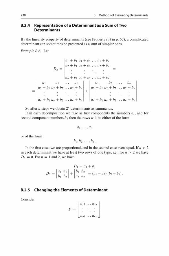
230 B Methods of Evaluating Determinants
B.2.4 Representation of a Determinant as a Sum of TwoDeterminants
By the linearity property of determinants (see Property (a) in p. 57), a complicateddeterminant can sometimes be presented as a sum of simpler ones.
Example B.6. Let
Dn D
ˇˇˇˇˇˇˇ
a1 C b1 a1 C b2 : : : a1 C bn
a2 C b1 a2 C b2 : : : a2 C bn
::::::
: : ::::
an C b1 an C b2 : : : an C bn
ˇˇˇˇˇˇˇ
D
D
ˇˇˇˇˇˇˇ
a1 a1 : : : a1
a2 C b1 a2 C b2 : : : a2 C bn
::::::
: : ::::
an C b1 an C b2 : : : an C bn
ˇˇˇˇˇˇˇC
ˇˇˇˇˇˇˇ
b1 b2 : : : bn
a2 C b1 a2 C b2 : : : a2 C bn
::::::
: : ::::
an C b1 an C b2 : : : an C bn
ˇˇˇˇˇˇˇ
So after n steps we obtain 2n determinants as summands.If in each decomposition we take as first components the numbers ai , and for
second component numbers bj then the rows will be either of the form
ai ; : : : ; ai
or of the formb1; b2; : : : ; bn:
In the first case two are proportional, and in the second case even equal. If n > 2
in each determinant we have at least two rows of one type, i.e., for n > 2 we haveDn D 0. For n D 1 and 2, we have
D1 D a1 C b1
D2 Dˇˇˇa1 a1
b1 b2
ˇˇˇC
ˇˇˇb1 b2
a2 a2
ˇˇˇ D .a1 � a2/ .b2 � b1/ :
B.2.5 Changing the Elements of Determinant
Consider
D D
66664
a11 : : : a1n
:::: : :
:::
an1 : : : ann
77775
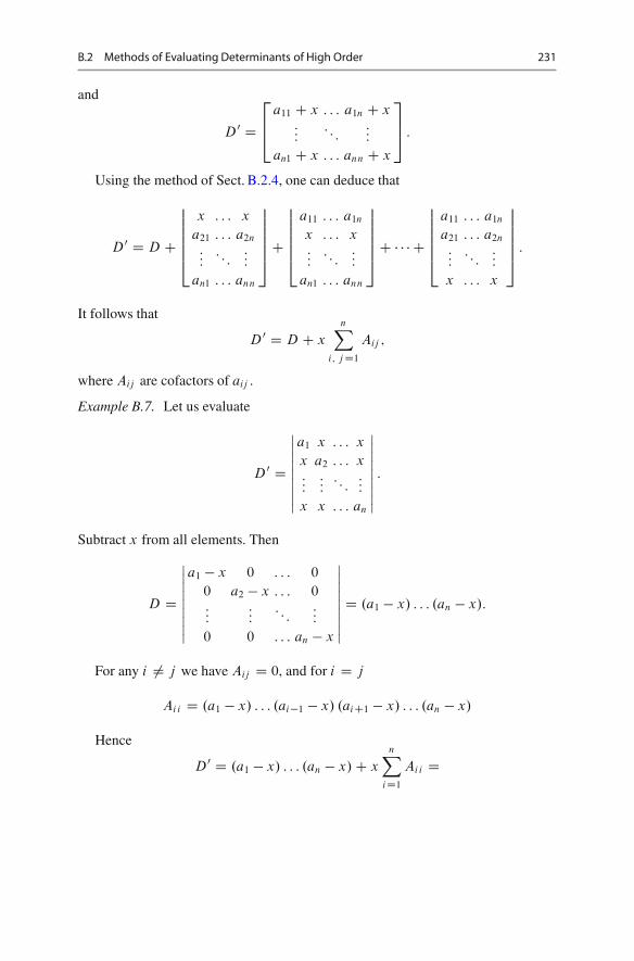
B.2 Methods of Evaluating Determinants of High Order 231
and
D0 D
2
64
a11 C x : : : a1n C x:::
: : ::::
an1 C x : : : ann C x
3
75 :
Using the method of Sect. B.2.4, one can deduce that
D0 D D C
6666664
x : : : x
a21 : : : a2n
:::: : :
:::
an1 : : : ann
7777775C
6666664
a11 : : : a1n
x : : : x:::
: : ::::
an1 : : : ann
7777775C � � � C
6666664
a11 : : : a1n
a21 : : : a2n
:::: : :
:::
x : : : x
7777775
:
It follows that
D0 D D C x
nX
i; j D1
Aij ;
where Aij are cofactors of aij .
Example B.7. Let us evaluate
D0 D
ˇˇˇˇˇˇˇ
a1 x : : : x
x a2 : : : x:::
:::: : :
:::
x x : : : an
ˇˇˇˇˇˇˇ:
Subtract x from all elements. Then
D D
ˇˇˇˇˇˇˇ
a1 � x 0 : : : 0
0 a2 � x : : : 0:::
:::: : :
:::
0 0 : : : an � x
ˇˇˇˇˇˇˇD .a1 � x/ : : : .an � x/:
For any i ¤ j we have Aij D 0, and for i D j
Aii D .a1 � x/ : : : .ai�1 � x/ .aiC1 � x/ : : : .an � x/
Hence
D0 D .a1 � x/ : : : .an � x/C x
nX
iD1
Aii D
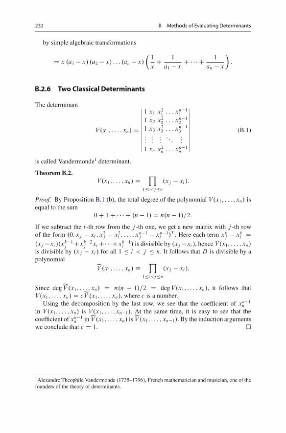
232 B Methods of Evaluating Determinants
by simple algebraic transformations
D x .a1 � x/ .a2 � x/ : : : .an � x/
�1
xC 1
a1 � xC � � � C 1
an � x
�:
B.2.6 Two Classical Determinants
The determinant
V.x1; : : : ; xn/ D
ˇˇˇˇˇˇˇˇˇ
1 x1 x21 : : : xn�1
1
1 x2 x22 : : : xn�1
2
1 x3 x23 : : : xn�1
3:::
::::::
: : ::::
1 xn x2n : : : xn�1
n
ˇˇˇˇˇˇˇˇˇ
(B.1)
is called Vandermonde1 determinant.
Theorem B.2.V.x1; : : : ; xn/ D
Y
1�i<j �n
.xj � xi /:
Proof. By Proposition B.1 (b), the total degree of the polynomial V.x1; : : : ; xn/ isequal to the sum
0C 1C � � � C .n� 1/ D n.n � 1/=2:
If we subtract the i -th row from the j -th one, we get a new matrix with j -th rowof the form .0; xj � xi ; x2
j � x2i ; : : : ; xn�1
j � xn�1i /T . Here each term xk
j � xki D
.xj �xi /.xk�1j Cxk�2
j xiC� � �Cxk�1i / is divisible by .xj �xi /, hence V.x1; : : : ; xn/
is divisible by .xj � xi / for all 1 � i < j � n. It follows that D is divisible by apolynomial
eV .x1; : : : ; xn/ �Y
1�i<j �n
.xj � xi /:
Since degeV .x1; : : : ; xn/ D n.n � 1/=2 D deg V.x1; : : : ; xn/, it follows thatV.x1; : : : ; xn/ D ceV .x1; : : : ; xn/, where c is a number.
Using the decomposition by the last row, we see that the coefficient of xn�1n
in V.x1; : : : ; xn/ is V.x1; : : : ; xn�1/. At the same time, it is easy to see that thecoefficient of xn�1
n in eV .x1; : : : ; xn/ is eV .x1; : : : ; xn�1/. By the induction argumentswe conclude that c D 1. �
1Alexandre Theophile Vandermonde (1735–1796), French mathematician and musician, one of thefounders of the theory of determinants.
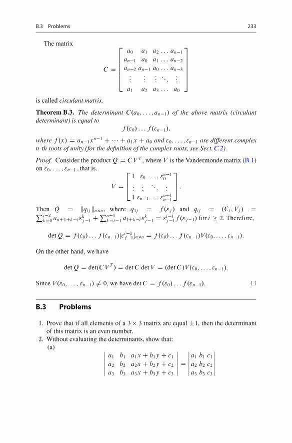
B.3 Problems 233
The matrix
C D
2
666664
a0 a1 a2 : : : an�1
an�1 a0 a1 : : : an�2
an�2 an�1 a0 : : : an�3
::::::
:::: : :
:::
a1 a2 a3 : : : a0
3
777775
is called circulant matrix.
Theorem B.3. The determinant C.a0; : : : ; an�1/ of the above matrix (circulantdeterminant) is equal to
f ."0/ : : : f ."n�1/;
where f .x/ D an�1xn�1 C � � � C a1x C a0 and "0; : : : ; "n�1 are different complexn-th roots of unity (for the definition of the complex roots, see Sect. C.2).
Proof. Consider the product Q D C V T , where V is the Vandermonde matrix (B.1)on "0; : : : ; "n�1, that is,
V D
2
64
1 "0 : : : "n�10
::::::
: : ::::
1 "n�1 : : : "n�1n�1
3
75 :
Then Q D kqij kn�n, where q1j D f ."j / and qij D .Ci ; Vj / DPi�2
kD0 anC1Ck�i "kj �1 C
Pn�1kDi�1 a1Ck�i "
kj �1 D "i�1
j �1f ."j �1/ for i � 2. Therefore,
det Q D f ."0/ : : : f ."n�1/j"i�1j �1jn�n D f ."0/ : : : f ."n�1/V ."0; : : : ; "n�1/:
On the other hand, we have
det Q D det.C V T / D det C det V D .det C /V."0; : : : ; "n�1/:
Since V."0; : : : ; "n�1/ ¤ 0, we have det C D f ."0/ : : : f ."n�1/. �
B.3 Problems
1. Prove that if all elements of a 3 � 3 matrix are equal ˙1, then the determinantof this matrix is an even number.
2. Without evaluating the determinants, show that:(a) ˇ
ˇˇˇˇ
a1 b1 a1x C b1y C c1
a2 b2 a2x C b2y C c2
a3 b3 a3x C b3y C c3
ˇˇˇˇˇDˇˇˇˇˇ
a1 b1 c1
a2 b2 c2
a3 b3 c3
ˇˇˇˇˇ
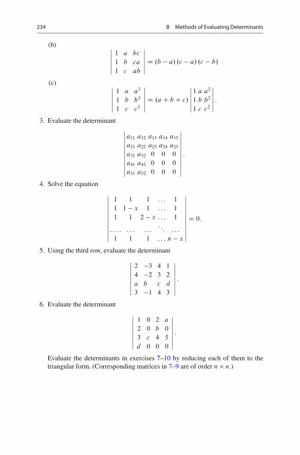
234 B Methods of Evaluating Determinants
(b) ˇˇˇˇˇ
1 a bc
1 b ca
1 c ab
ˇˇˇˇˇD .b � a/ .c � a/ .c � b/
(c) ˇˇˇˇˇ
1 a a3
1 b b3
1 c c3
ˇˇˇˇˇD .aC b C c/
ˇˇˇˇˇ
1 a a2
1 b b2
1 c c2
ˇˇˇˇˇ:
3. Evaluate the determinantˇˇˇˇˇˇˇˇˇ
a11 a12 a13 a14 a15
a21 a22 a23 a24 a25
a31 a32 0 0 0
a41 a42 0 0 0
a51 a52 0 0 0
ˇˇˇˇˇˇˇˇˇ
:
4. Solve the equation
ˇˇˇˇˇˇˇˇˇˇ
1 1 1 : : : 1
1 1 � x 1 : : : 1
1 1 2 � x : : : 1
: : : : : : : : : :: : : : : :
1 1 1 : : : n � x
ˇˇˇˇˇˇˇˇˇˇ
D 0:
5. Using the third row, evaluate the determinant
ˇˇˇˇˇˇ
2 �3 4 1
4 �2 3 2
a b c d
3 �1 4 3
ˇˇˇˇˇˇ
:
6. Evaluate the determinant
ˇˇˇˇˇˇˇ
1 0 2 a
2 0 b 0
3 c 4 5
d 0 0 0
ˇˇˇˇˇˇˇ
:
Evaluate the determinants in exercises 7–10 by reducing each of them to thetriangular form. (Corresponding matrices in 7–9 are of order n � n.)

B.3 Problems 235
7. ˇˇˇˇˇˇˇˇˇ
1 1 1 : : : 1
1 1 0 : : : 0
1 0 1 : : : 0:::
::::::
: : ::::
1 0 0 : : : 1
ˇˇˇˇˇˇˇˇˇ
:
8. ˇˇˇˇˇˇˇˇˇ
1 1 1 : : : 1
1 0 1 : : : 1
1 1 0 : : : 1:::
::::::
: : ::::
1 1 1 : : : 0
ˇˇˇˇˇˇˇˇˇ
:
9. ˇˇˇˇˇˇˇˇˇ
3 2 2 : : : 2
2 3 2 : : : 2
2 2 3 : : : 2
: : : : : : : : : :: : : : : :
2 2 2 : : : 3
ˇˇˇˇˇˇˇˇˇ
:
10. ˇˇˇˇˇˇˇˇˇ
a0 a1 a2 : : : an
�x x 0 : : : 0
0 �x x : : : 0
: : : : : : : : : :: : : : : :
0 0 0 : : : x
ˇˇˇˇˇˇˇˇˇ
:
Evaluate the determinants in questions 11 and 12 (by using linear multipliers).11. ˇ
ˇˇˇˇˇˇˇˇˇ
a0 a1 a2 : : : an
a0 x a2 : : : an
a0 a1 x : : : an
::::::
:::: : :
:::
a0 a1 a2 : : : x
ˇˇˇˇˇˇˇˇˇˇ
12. ˇˇˇˇˇˇ
�x a b c
a �x c b
b c �x a
c b a �x
ˇˇˇˇˇˇ
Evaluate the determinants in questions 13–15 by using the recursive definition.(Corresponding matrices in Problems 14 and 15 are of order n � n.)

236 B Methods of Evaluating Determinants
13. ˇˇˇˇˇˇˇˇˇ
a1 1 1 : : : 1
1 a2 0 : : : 0
1 0 a3 : : : 0:::
::::::
: : ::::
1 0 0 : : : an
ˇˇˇˇˇˇˇˇˇ
14. ˇˇˇˇˇˇˇˇˇ
2 1 0 : : : 0
1 2 1 : : : 0
0 1 2 : : : 0:::
::::::
: : ::::
0 0 0 : : : 2
ˇˇˇˇˇˇˇˇˇ
15. ˇˇˇˇˇˇˇˇˇ
3 2 0 : : : 0
1 3 2 : : : 0
0 1 3 : : : 0:::
::::::
: : ::::
0 0 0 : : : 3
ˇˇˇˇˇˇˇˇˇ
16. Evaluate the following determinant representing it as a sum of determinants:
ˇˇˇˇˇˇˇˇ
x1 a2 : : : an
a1 x2 : : : an
::::::
: : ::::
a1 a2 : : : xn
ˇˇˇˇˇˇˇˇ
Hint: insert xi D .xi � ai /C ai .17. Let x0; x1; : : : ; xn are variables and p0; p1; : : : ; pn are polynomials of the form
pj D aj xj C (lower terms). Show that
ˇˇˇˇˇ
p0.x0/ p1.x0/ : : : pn.x0/:::
:::: : :
:::
p0.xn/ p1.xn/ : : : pn.xn/
ˇˇˇˇˇD a0 : : : anV .x0; : : : ; xn/:
CComplex Numbers
Besides the dot product, in the plane R2 there is another product of vectors, calledcomplex multiplication. In contrast to the dot product, the complex product of twovectors is again a vector in R2. It is given by the formula
.x; y/.x0; y0/ D .xx0 � yy0; xy0 C yx0/:
The properties of complex multiplication (given below) are close to the usualmultiplication of real numbers, and the elements of R2 are referred as complexnumbers. The set R2 of complex numbers is also denoted by C. In particular, thevectors in the horizontal axis are identified with real numbers, that is, the realnumber x corresponds to the vector .x; 0/ (therefore, we have R � C). For example,the number 1 is identified with the vector .1; 0/, the first vector of the canonicalbasis. The horizontal axis is called a real axis. The sum (product) of two realnumbers a and b is identified with the sum (product) of corresponding complexnumbers .a; 0/ and .b; 0/, so that one can consider the complex numbers as anextension of the real number system.
The second vector of the canonical basis .0; 1/, being considered as a complexnumber, is denoted by i and called a imaginary unit, or the square root of �1
(because i 2 D .�1; 0/ D �1). The vertical axis is called an imaginary axis, andevery vector of the form .0; x/ D x � i is called a pure imaginary number. It followsthat any complex number z D .x; y/ is a sum of a real number and a pure imaginarynumber, that is,
z D .x; y/ D x.1; 0/C y.0; 1/ D x C yi:
The first entry x is called a real part of z and denoted as <z. The second entry y iscalled an imaginary part of z and denoted as =z.
F. Aleskerov et al., Linear Algebra for Economists, Springer Texts in Businessand Economics, DOI 10.1007/978-3-642-20570-5,© Springer-Verlag Berlin Heidelberg 2011
237
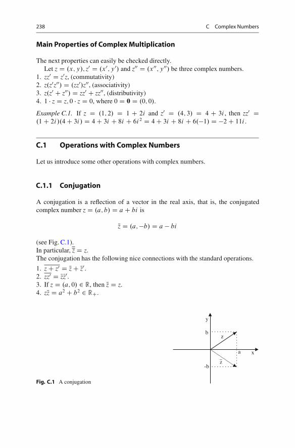
238 C Complex Numbers
Main Properties of Complex Multiplication
The next properties can easily be checked directly.Let z D .x; y/; z0 D .x0; y0/ and z00 D .x00; y00/ be three complex numbers.
1. zz0 D z0z, (commutativity)2. z.z0z00/ D .zz0/z00, (associativity)3. z.z0 C z00/ D zz0 C zz00, (distributivity)4. 1 � z D z; 0 � z D 0, where 0 D 0 D .0; 0/.
Example C.1. If z D .1; 2/ D 1 C 2i and z0 D .4; 3/ D 4 C 3i , then zz0 D.1C 2i/.4C 3i/ D 4C 3i C 8i C 6i2 D 4C 3i C 8i C 6.�1/ D �2C 11i .
C.1 Operations with Complex Numbers
Let us introduce some other operations with complex numbers.
C.1.1 Conjugation
A conjugation is a reflection of a vector in the real axis, that is, the conjugatedcomplex number z D .a; b/ D aC bi is
Nz D .a;�b/ D a � bi
(see Fig. C.1).In particular, z D z.The conjugation has the following nice connections with the standard operations.
1. zC z0 D NzC Nz0.2. zz0 D NzNz0.3. If z D .a; 0/ 2 R, then Nz D z.4. zNz D a2 C b2 2 RC.
Fig. C.1 A conjugation
x
y
z
z
a
-b
b

C.1 Operations with Complex Numbers 239
One can express the real and imaginary parts of a complex number via conjuga-tion as
<z D .1=2/.zC Nz/and
=z D .i=2/.Nz� z/:
C.1.2 Modulus
The modulus jzj of a complex number z D .a; b/ is its length as a vector in R2, thatis,
jzj Dp
a2 C b2 D pzNz:The modulus of the product of two complex numbers is the product of their moduli,that is,
jzz0j D jzjjz0j(because jzjjz0j D pzNz
pz0z0 D
pzz0zz0 D jzz0j).
Example C.2. j3 C 4i j Dq
.3C 4i/.3C 4i/ D p.3C 4i/.3� 4i/ Dp
32 C 42 D 5.
C.1.3 Inverse and Division
The inverse of a nonzero complex number z D a C bi is defined as z�1 D jzj�2Nz.Then z�1z D jzj�2Nzz D jzj�2jzj2 D 1, so that one can define a division of complexnumbers as z0=z D z0z�1 D jzj�2z0Nz, that is,
a0 C b0iaC bi
D .a0 C b0i/.a � bi/
.aC bi/.a � bi/D .a2 C b2/�1.a0 C b0i/.a � bi/:
Note that the denominator z D aC bi must be nonzero.
Example C.3.
18C i
3 � 4iD .18C i/.3C 4i/
.3 � 4i/.3C 4i/D 50C 75i
32 C 42D 2C 3i:
C.1.4 Argument
An argument of a nonzero complex number z D aCbi is an angle ' between the realaxis and the vector z (see Fig. C.2). Obviously, sin ' D b=jzj and cos ' D a=jzj, so,' is defined uniquely up to the period 2� . The set of all such possible � is denoted
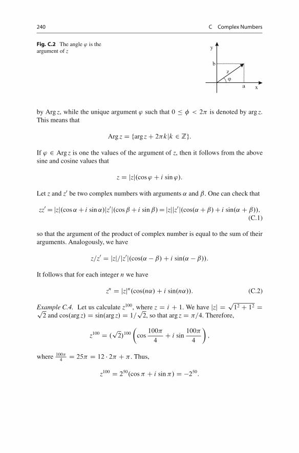
240 C Complex Numbers
Fig. C.2 The angle ' is theargument of z
x
y
a
b
zϕ
by Arg z, while the unique argument ' such that 0 � � < 2� is denoted by arg z.This means that
Arg z D farg zC 2�kjk 2 Zg:
If ' 2 Arg z is one the values of the argument of z, then it follows from the abovesine and cosine values that
z D jzj.cos ' C i sin '/:
Let z and z0 be two complex numbers with arguments ˛ and ˇ. One can check that
zz0Djzj.cos ˛C i sin ˛/jz0j.cos ˇC i sin ˇ/Djzjjz0j.cos.˛Cˇ/C i sin.˛ C ˇ//;
(C.1)
so that the argument of the product of complex number is equal to the sum of theirarguments. Analogously, we have
z=z0 D jzj=jz0j.cos.˛ � ˇ/C i sin.˛ � ˇ//:
It follows that for each integer n we have
zn D jzjn.cos.n˛/C i sin.n˛//: (C.2)
Example C.4. Let us calculate z100, where z D i C 1. We have jzj D p12 C 12 Dp2 and cos.arg z/ D sin.arg z/ D 1=
p2, so that arg z D �=4. Therefore,
z100 D .p
2/100
�cos
100�
4C i sin
100�
4
�;
where 100�4D 25� D 12 � 2� C � . Thus,
z100 D 250.cos � C i sin �/ D �250:
C.2 Algebraic Equations 241
C.1.5 Exponent
The exponent of a complex number z D aC bi is defined as
eaCbi D ea.cosb C i sin b/
(Euler1 formula). It follows that for each nonzero complex z we have
z D jzjei arg z:
Example C.5. ei� D e0.cos� C i sin �/ D �1.
Other properties of exponents of complex numbers follows from the equa-tion (C.1):
ezCz0 D ezez0
; e�z D 1=ez; ez�z0 D ez=ez0
:
C.2 Algebraic Equations
Many equations which have no real solutions have complex ones. The simplestexample is the equation z2 C 1D 0, which has two complex solutions, zD i andzD � i , and no real ones. More generally, each quadratic equation
ax2 C bx C c D 0
with real coefficients a; b and c always have complex solutions xD�b ˙
pb2 � 4ac
2a, where in the case DD b2 � 4ac < 0 we take
pDD i
pjDj.Moreover, some simple algebraic equations have quite more complex solutions
than real ones. Consider an equation
zn D c;
where c is a nonzero complex number. If arg z D ˛ and arg c D �, the formula (C.2)gives the equation
jzjn.cos.n˛/C i sin.n˛// D jcj.cos � C i sin �/;
1Leonhard Euler (1707–1783) was a great Swiss mathematician who made enormous contributionsto a wide range of mathematics and physics including analytic geometry, trigonometry, geometry,calculus and number theory. Most of his life he had been working in Russia (St. Petersburg) andPrussia (Berlin).
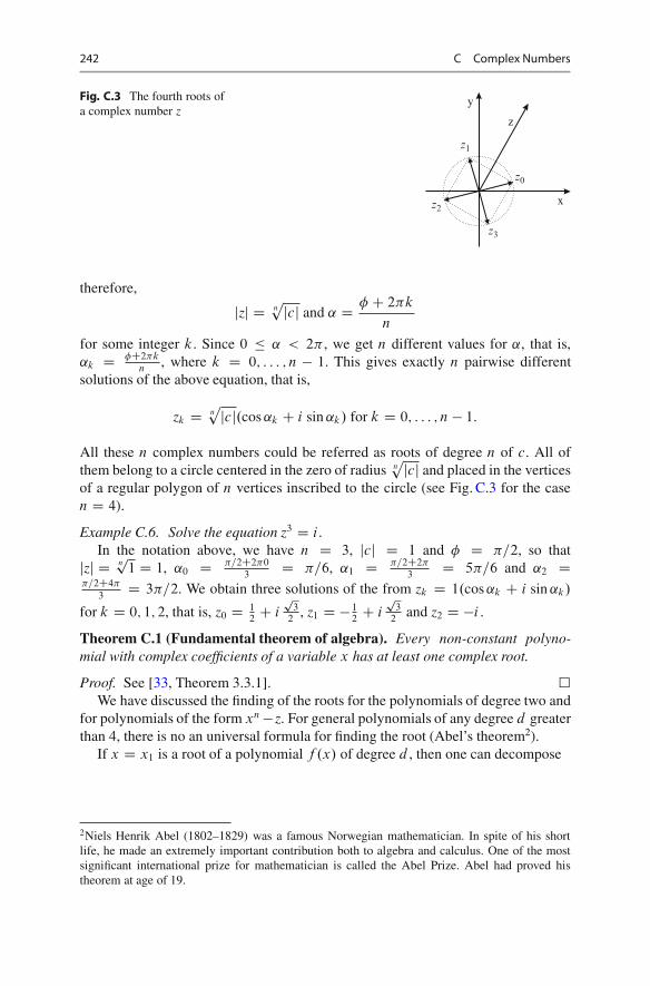
242 C Complex Numbers
Fig. C.3 The fourth roots ofa complex number z
z
x
y
z0
z1
z2
z3
therefore,
jzj D npjcj and ˛ D � C 2�k
n
for some integer k. Since 0 � ˛ < 2� , we get n different values for ˛, that is,˛k D �C2�k
n, where k D 0; : : : ; n � 1. This gives exactly n pairwise different
solutions of the above equation, that is,
zk D npjcj.cos ˛k C i sin ˛k/ for k D 0; : : : ; n � 1:
All these n complex numbers could be referred as roots of degree n of c. All ofthem belong to a circle centered in the zero of radius n
pjcj and placed in the verticesof a regular polygon of n vertices inscribed to the circle (see Fig. C.3 for the casen D 4).
Example C.6. Solve the equation z3 D i .In the notation above, we have n D 3, jcj D 1 and � D �=2, so that
jzj D np
1 D 1, ˛0 D �=2C2�03
D �=6, ˛1 D �=2C2�3
D 5�=6 and ˛2 D�=2C4�
3D 3�=2. We obtain three solutions of the from zk D 1.cos ˛k C i sin ˛k/
for k D 0; 1; 2, that is, z0 D 12C i
p3
2, z1 D � 1
2C i
p3
2and z2 D �i .
Theorem C.1 (Fundamental theorem of algebra). Every non-constant polyno-mial with complex coefficients of a variable x has at least one complex root.
Proof. See [33, Theorem 3.3.1]. �We have discussed the finding of the roots for the polynomials of degree two and
for polynomials of the form xn� z. For general polynomials of any degree d greaterthan 4, there is no an universal formula for finding the root (Abel’s theorem2).
If x D x1 is a root of a polynomial f .x/ of degree d , then one can decompose
2Niels Henrik Abel (1802–1829) was a famous Norwegian mathematician. In spite of his shortlife, he made an extremely important contribution both to algebra and calculus. One of the mostsignificant international prize for mathematician is called the Abel Prize. Abel had proved histheorem at age of 19.

C.2 Algebraic Equations 243
f .x/ D .x � x1/g.x/;
where g.x/ is another polynomial of degree d � 1 (with complex coefficients). Ifthe degree d � 1 is positive, the polynomial g.x/ must have another complex root,say, x2. Proceeding such decomposition up to degree 0, we get the decompositionof the from
f .x/ D c.x � x1/.x � x2/ : : : .x � xd /;
where c is a complex number and x1; : : : ; xd are roots of the polynomial f .x/.Combining the identical terms, we get (after a possible re-numerating of xi ’s) thedecomposition
f .x/ D c.x � x1/k1.x � x2/k2 : : : .x � xs/ks
for some s � d , where the sum of the powers k1C � � �C ks is d . Each number kj iscalled a multiplicity of the corresponding root xj . The roots of multiplicity one arecalled simple. One can check that each root xj of the polynomial should appear inthis decomposition.
We have
Corollary C.2. The number of roots of any polynomial p.x/ of degree d > 0 is notgreater than d . Moreover, the sum of all multiplicities of the roots is equal to d .
Example C.7. Problem. Solve the equation z2 � 4iz� 7 � 4i D 0.
Solution. By the well-known formula (which is easy to be checked), the numberz D �.�4i/Cd
2satisfies the equation, where d 2 D .�4i/2� 4.�7� 4i/ D 12C 16i .
We need to find d . Let d D x C iy, where x and y are real numbers. Then d 2 D.x2 � y2/C 2ixy, so that the equality of two 2-dimensional vectors d 2 D 12C 16i
gives a system of two equations
�x2 � y2 D 12;
2xy D 16:
This system has two solutions for d D xCiy, that is, d1 D 4C2i and d2 D �4�2i .This leads us to two roots of the equation above: z1 D .4i C d1/=2 D 2C 3i andz2 D .4i C d2/=2 D �2C i . Since the equation has degree two, there are no otherroots but these two.
To find a decomposition of a polynomial with real coefficients, the followingstatement is often useful.
Theorem C.3. If a complex number z is a root of a polynomial f .x/ with realcoefficients, then the conjugated number Nz is also a root of f .x/. Moreover, themultiplicities of these roots are the same.
Proof. If f .x/ D ad xd C � � � C a1xC a0 and f .z/ D 0, then f .Nz/ D ad Nzd C � � � Ca1NzC a0 D Nad Nzd C � � � C Na1Nz C Na0 D ad zd C � � � C a1z C a0 D f .z/ D N0 D 0.
244 C Complex Numbers
The claim about the multiplicities follows from the induction argument applied tothe polynomial g.x/ of degree d � 2 such that f .x/ D .x � z/.x � Nz/g.x/. �
Example C.8. Let us find the decomposition of a polynomial f .z/ D z4 � 5z3 C7z2�5zC6. One can check that f .i/ D 0, so that z D i is a root of the polynomial.If follows that the number Nz D �i is another root. From the decomposition
f .z/ D .z� i/.zC i/g.z/
one can find g.z/ D z2 � 5zC 6. It follows that g.z/ D .z � 2/.z� 3/, so that
f .z/ D .z� i/.zC i/.z � 2/.z � 3/:
C.3 Linear Spaces Over Complex Numbers
Recall from the definition in the beginning of Chap. 6 that a linear space is a setadmitting two operations, that is, addition and multiplication by a real number (dotproduct) such that these operations satisfies the linearity properties. One can extendthis definition by allowing the multiplication of by complex numbers, not only byreal ones. Such a vector space is called a vector space over complex numbers, orsimply a complex vector space. In contrast, the vector space in the sense of Chap. 6is called a vector space over real numbers, or a real vector space. The definition ofcomplex vector space repeats the definition of real one literally but the world ‘real’is replaced by ‘complex’.
The notions of linear dependence and independence of vectors, dimension andbasis of a vector space, subspace, isomorphism etc. for complex vector spaces repeatthe correspondent definitions given in Chap. 6 verbatim. The definition and theproperties of linear transformation and its matrix from Chap. 8 are transferred tothe case of complex vector spaces verbatim as well.
Example C.9. The set C itself is a one-dimensional complex vector space. Any itsnonzero element z D aC bi ¤ 0 form a basis of it, since for each w D xCyi 2 C
one has w D ˛z, where ˛ D w=z 2 C.
Example C.10. The set Cn of n-tuples of complex numbers x D .x1; : : : ; xn/ withx1; : : : ; xn 2 C is an n-dimensional vector space with standard operations
.x1; : : : ; xn/C .y1; : : : ; yn/ D .x1 C y1; : : : ; xn C yn/
and˛.x1; : : : ; xn/ D .˛x1; : : : ; ˛xn/:
Its dimension is equal to n by the same reason as for the real space Rn, seeExample 6.5.

C.4 Problems 245
Given a real vector space V , one can embed it in a complex vectors space bythe following way. Let V C be the set of pairs of vectors from V . Each such pair wedenote by .u; v/ D uCiv. The addition of pairs and their multiplication by complexnumbers are defined as
.uC iv/C .u0 C iv0/ D .uC u0/C i.vC v0/
and.aC bi/.uC iv/ D .au � bv/C i.avC bu/:
Exercise C.1. Show that V C is a linear space over complex numbers.
Such a complex vector space V C is called a complexification of V .
Example C.11. C D RC and Cn D .Rn/C.
Given a vector w D u C iv in a complexification V C, one can define its realand imaginary parts as <w D u and =w D v, the both are vectors in the realvector space V . Any basis of V is also a basis of the complexification V C, butone can also construct other bases in V C which do not belong to V . For any lineartransformation f W U ! V of two real vector spaces U and V , one can also defineits complexification f C W U C ! V C by the obvious formula f C.u C iv/ Df .u/C if .v/. Note that if we fix two bases in the real vector spaces U and V , thenthe matrices of the linear transformations f and f C in these bases are the same.
In particular, we prove in Corollary 9.5 that any linear operator in a finite-dimensional complex vector space has an eigenvector. This means that if f isa linear operator in a real vector space V , then its complexification f C has aneigenvector in V C. In particular, it follows that the matrix of f has an eigenvalue.
C.4 Problems
1. Calculate.1C i/.2C i/
3 � i:
2. Calculatei � 3
2 � 3iC i C 3
2C 3i:
3. Calculate.1C i/4
.i � 1/5:
4. Solve the system of linear equations with complex coefficients
�.1C 2i/x � 2iy D 5C 9i
.�1C 3i/x C .1C i/y D �6C 4i:

246 C Complex Numbers
5. Find all real solutions of the equation
.2i � 2/x � .i C 1/y D 2i � 10:
6. Solve the equation
z2 C 2zC 37 D 0:
7. Solve the equation
iz2 C .3i � 2/zC 12C 4i D 0:
8. Solve the equation
z2 C 6z � 4izC 5 � 12i D 0:
9. Solve the equation
z2 � 5zC 4izC 9 � i D 0:
10. Calculate i 100.11. Calculate .1 � i/n, where n is a positive integer.12. Solve the equation z6 D i .13. Solve the equation z4 D �128C 128
p3i .
14. Plot all the solutions of the equation z6 D 117C 44i in the complex plane.15. Find all solutions of the equation z5 D 5e5i .16. Find the multiplicity of the root z D 2 of the polynomial z5 � 6z4 C 13z3 �
14z2 C 12z� 8.17. Find the multiplicity of the root z D i C 1 of the polynomial z5 � 6z4 C 16z3 �
24z2 C 20z� 8.18. Prove that jz1 C z2j � jz1j C jz2j.19. Prove the equation (C.1).20. Let z and z0 be two nonzero vectors in R2 (that is, complex numbers) such thatjzj D jz0j and z ? z0. Find all possible values of z0=z.
21. Let "0; : : : ; "n�1 be different complex n-th roots of unity, where n � 2. Showthat "0 C � � � C "n�1 D 0 and "0 : : : "n�1 D .�1/n�1.
22. Prove that ez1Cz2 D ez1ez2 .23. Solve the equation ez D e for a complex number z.24. Let A be a linear operator in C2 given by the matrix
�1 2
3 4
�:
C.4 Problems 247
Find its matrix in the basis
f1 D .i; 1/; f2 D .1; i/:
25. Let V be an n-dimensional complex vector space. Show that V is also a realvector space, where the multiplication by the real numbers is defined by thesame way as the multiplication by complex ones (as the real numbers form asubspace of complex numbers). Find the dimension of V as a real vector space.

•
DPseudoinverse
Consider a general linear system
Ax D b: (D.1)
If the matrix A is square and non-singular, we have the solution
x D A�1b:
But if A is singular or even non-square, problems of two types arise. First, if thesystem (D.1) is consistent and the rank of A is less than the number of variables,we have a multiple solution which can be found algorithmically by, say, Gaussianelimination (see Sect. 5.2). But in many practical problems, we need an explicitformula for a (particular) solution depending on the vector b in the right side. Howto get such an explicit formula?
Second, a problem arises if the system (D.1) is inconsistent. In practicalproblems, we need in this case an approximate solution (see Sect. (7.3)). Is therea formula for expressing it?
An answer to the both questions is given by a construction due to Moore1 andPenrose2 called a pseudoinverse3. For many generalizations and applications of thisconstruction, we refer the reader to [2, 5].
1Eliakim Hastings Moore (1862–1932), an American mathematician who made a significantcontribution to algebra and logics. In 1935, he gave a definition pseudoinverse under the namegeneral reciprocal.2Roger Penrose (1931) is a famous English physicists and mathematician. He was awarded theWolf foundation prise (1988, shared with Stephen Hawking) for the work which has “greatlyenlarged our understanding of the origin and possible fate of the Universe”. In 1955, he re-discovered the Moore definition of the pseudoinverse and demonstrated its connection with theleast square approximation.3The terms generalized inverse and Moore–Penrose inverse are also used.
F. Aleskerov et al., Linear Algebra for Economists, Springer Texts in Businessand Economics, DOI 10.1007/978-3-642-20570-5,© Springer-Verlag Berlin Heidelberg 2011
249

250 D Pseudoinverse
D.1 Definition and Basic Properties
Definition D.1. Let A be an m�n matrix. The matrix AC is called a pseudoinverse4
of A if the following four conditions hold
1: AACA D A
2: ACAAC D AC
3:AACT D AAC
4:ACA
T D ACA:
Later (see Theorem D.5) we will show that every matrix A admits a pseudoin-verse.
Note that since both ACA and AAC exist, AC must be an m � n matrix.The first property give us the right to call it the pseudoinverse.
Theorem D.1. Let A be a matrix. If its pseudoinverse exists, then it is unique.
Proof. Suppose B and C are two pseudoinverses of A, that is, both matrices B andC satisfy the conditions (1–4) of Definition D.1. Then we have:
AB D .ACA/B D .AC /.AB/ D .AC /T .AB/T
D C T AT BT AT D C T .ABA/T D C T AT D .AC /T D AC:
By the same way, we have
BA D B.ACA/ D .BA/.CA/ D .BA/T .CA/T
D AT BT AT C T D .ABA/T C T D AT C T D .CA/T D CA:
ThusB D BAB D .BA/B D .CA/B D C.AB/ D CAC D C:
�
Example D.1. Suppose that A is a non-singular square matrix. Then the pseudoin-verse AC exists and
AC D A�1:
Proof. We have AA�1A D AI D A and A�1AA�1 D A�1I D A�1. If A is oforder n, then A�1 is of order n as well, so that
4There are other versions of definition of generalized inverse, or pseudoinverse, matrix. The mostuseful of the definitions require only some of the Penrose conditions (1–4) from Definition D.1,e.g., (1) and (2). On the definitions and properties of these more general versions of inverse matrix,see [5, Chap. 6] and [2]; see also [8, pp. 94–98], [26, pp. 203–205].
D.1 Definition and Basic Properties 251
AA�1 D In D A�1A:
This means that the matrix A�1 satisfies the conditions (1–4) of Definition D.1. �
Example D.2. Let
A D
2
64
a1
:::
an
3
75
be a nonzero column vector. Then the row vector
C D �AT
is a pseudoinverse of A, where � D 1=.a21 C � � � C a2
n/.
Proof. We have AC D �.ai aj /n�n and CA D �.AAT / D 1, so that theconditions (3) and (4) hold for the matrix C . In addition, we have ACA D A1 D A
and CAC D 1C D C , so that the conditions (1) and (2) hold as well. �
Example D.3. Suppose that an m � n matrix A has the form
A D"
B 0
0 0
#
;
where B is an r � r non-singular submatrix. Then the pseudoinverse AC is an n�m
matrix of the form
C D"
B�1 0
0 0
#
:
Proof. It is easy to see that AC and CA are square matrices of the form
"Ir 0
0 0
#
of orders m and n, respectively. It follows that .AC /T D AC and .CA/T D CA.According to Lemma 9.16, we have ACA D .AC /A D A and CAC D .CA/C DC . By Definition D.1, this means that AC D C is the pseudoinverse. �
D.1.1 The Basic Properties of Pseudoinverse
5: .AC/C D A
6: .AT /C D .AC/T
252 D Pseudoinverse
Proof. Exercise. �7: rank AC D rank A
Proof. Recall that rank.AB/ � rank A and rank.AB/ � rank B for any twomatrices A and B conformable for multiplication (see Problem 24 in Chap. 2). Then
rank A D rank.AACA/ � rank.AAC/ � rank AC
andrank AC D rank.ACAAC/ � rank.AAC/ � rank A:
�
Exercise D.1. Show that if rank A D 1, then AC D 1Tr.AAT /
AT :
Hint. If rank A D 1, then all columns of A are linear combinations of a singlecolumn, say, Ak , that is,
A D .�1Akj : : : j�nAk/ D .�1; : : : ; �n/Ak:
D.2 Full Rank Factorization and a Formula for Pseudoinverse
Let us give the formula for a pseudoinverse of a matrix with linearly independentcolumns.
Theorem D.2. Suppose that an m � n matrix A has full column rank, that is,rank A D n. Then A has a pseudoinverse
AC D .AT A/�1AT :
We begin with
Lemma D.3. Let A be an m�n with full column rank. Then the n�n matrix AT A
is non-singular.
Proof. Suppose that rank.AT A/ < n. By Theorem 5.6, it follows that the system
AT Ax D 0
has a nonzero solution x. Then
xT AT Ax D 0;
.Ax/T Ax D 0;
that is, .Ax; Ax/ D 0. Hence Ax D 0. Since x ¤ 0, we have rank A < n, acontradiction. �
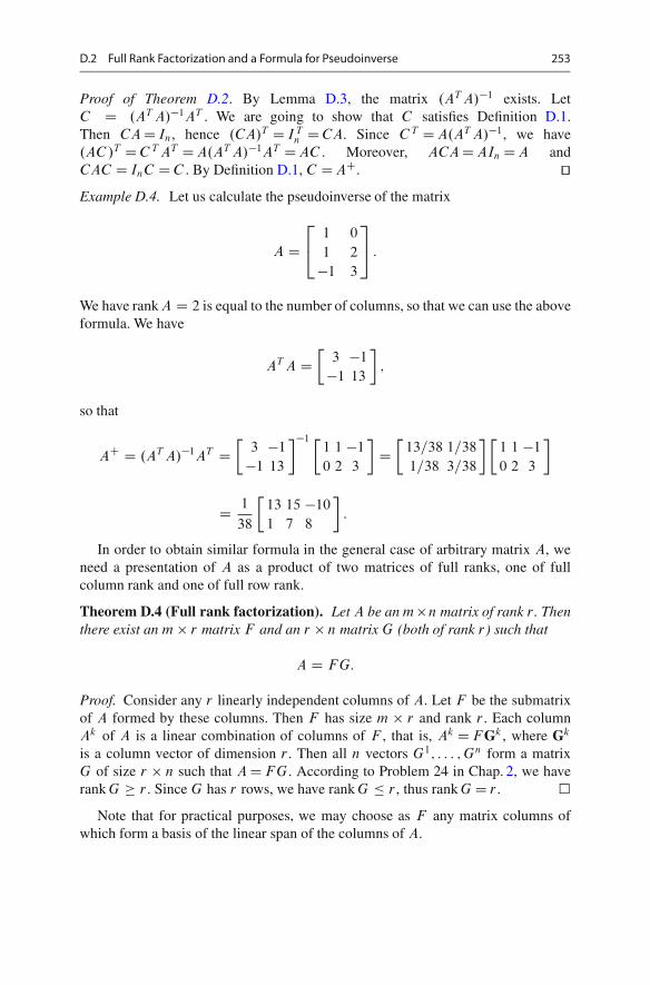
D.2 Full Rank Factorization and a Formula for Pseudoinverse 253
Proof of Theorem D.2. By Lemma D.3, the matrix .AT A/�1 exists. LetC D .AT A/�1AT . We are going to show that C satisfies Definition D.1.Then CAD In, hence .CA/T D I T
n DCA. Since C T DA.AT A/�1, we have.AC /T DC T AT DA.AT A/�1AT DAC . Moreover, ACADAInDA andCAC D InC DC . By Definition D.1, C DAC. utExample D.4. Let us calculate the pseudoinverse of the matrix
A D2
41 0
1 2
�1 3
3
5 :
We have rank A D 2 is equal to the number of columns, so that we can use the aboveformula. We have
AT A D�
3 �1
�1 13
�;
so that
AC D .AT A/�1AT D�
3 �1
�1 13
��1 �1 1 �1
0 2 3
�D�
13=38 1=38
1=38 3=38
� �1 1 �1
0 2 3
�
D 1
38
�13 15 �10
1 7 8
�:
In order to obtain similar formula in the general case of arbitrary matrix A, weneed a presentation of A as a product of two matrices of full ranks, one of fullcolumn rank and one of full row rank.
Theorem D.4 (Full rank factorization). Let A be an m�n matrix of rank r . Thenthere exist an m � r matrix F and an r � n matrix G (both of rank r) such that
A D F G:
Proof. Consider any r linearly independent columns of A. Let F be the submatrixof A formed by these columns. Then F has size m � r and rank r . Each columnAk of A is a linear combination of columns of F , that is, Ak DF Gk , where Gk
is a column vector of dimension r . Then all n vectors G1; : : : ; Gn form a matrixG of size r � n such that ADF G. According to Problem 24 in Chap. 2, we haverank G � r . Since G has r rows, we have rank G � r , thus rank GD r . �
Note that for practical purposes, we may choose as F any matrix columns ofwhich form a basis of the linear span of the columns of A.
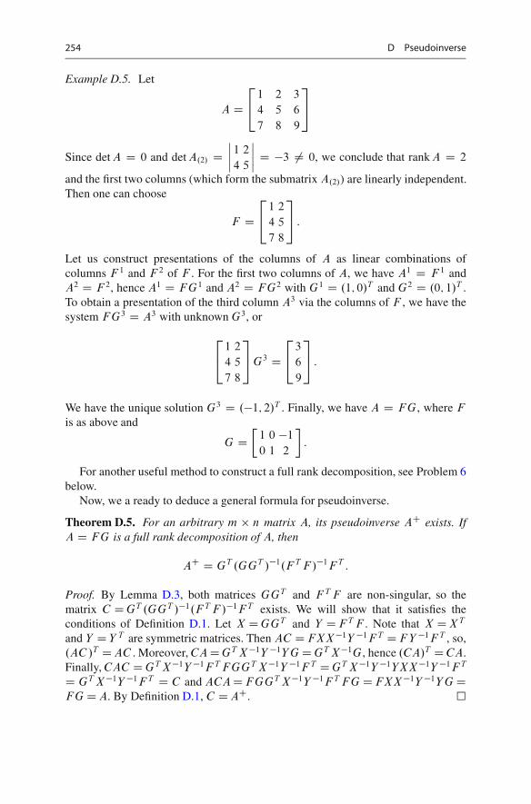
254 D Pseudoinverse
Example D.5. Let
A D2
41 2 3
4 5 6
7 8 9
3
5
Since det A D 0 and det A.2/ Dˇˇˇˇ1 2
4 5
ˇˇˇˇ D �3 ¤ 0, we conclude that rank A D 2
and the first two columns (which form the submatrix A.2/) are linearly independent.Then one can choose
F D2
41 2
4 5
7 8
3
5 :
Let us construct presentations of the columns of A as linear combinations ofcolumns F 1 and F 2 of F . For the first two columns of A, we have A1 D F 1 andA2 D F 2, hence A1 D F G1 and A2 D F G2 with G1 D .1; 0/T and G2 D .0; 1/T .To obtain a presentation of the third column A3 via the columns of F , we have thesystem F G3 D A3 with unknown G3, or
2
41 2
4 5
7 8
3
5G3 D2
43
6
9
3
5 :
We have the unique solution G3 D .�1; 2/T . Finally, we have A D F G, where F
is as above and
G D�
1 0 �1
0 1 2
�:
For another useful method to construct a full rank decomposition, see Problem 6below.
Now, we a ready to deduce a general formula for pseudoinverse.
Theorem D.5. For an arbitrary m � n matrix A, its pseudoinverse AC exists. IfA D F G is a full rank decomposition of A, then
AC D GT .GGT /�1.F T F /�1F T :
Proof. By Lemma D.3, both matrices GGT and F T F are non-singular, so thematrix C DGT .GGT /�1.F T F /�1F T exists. We will show that it satisfies theconditions of Definition D.1. Let X DGGT and Y DF T F . Note that X DXT
and Y DY T are symmetric matrices. Then AC DFXX�1Y �1F T DF Y �1F T , so,.AC /T DAC . Moreover, CADGT X�1Y �1Y GDGT X�1G, hence .CA/T DCA.Finally, CAC DGT X�1Y �1F T F GGT X�1Y �1F T DGT X�1Y �1YXX�1Y �1F T
D GT X�1Y �1F T D C and ACADF GGT X�1Y �1F T F GDFXX�1Y �1Y GDF GDA. By Definition D.1, C DAC. �
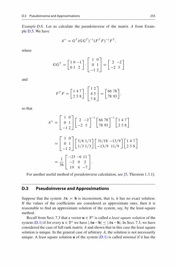
D.3 Pseudoinverse and Approximations 255
Example D.6. Let us calculate the pseudoinverse of the matrix A from Exam-ple D.5. We have
AC D GT .GGT /�1.F T F /�1F T ;
where
GGT D�
1 0 �1
0 1 2
��2
41 0
0 1
�1 2
3
5 D�
2 �2
�2 5
�
and
F T F D�
1 4 7
2 5 8
��2
41 2
4 5
7 8
3
5 D�
66 78
78 93
�;
so that
AC D2
41 0
0 1
�1 2
3
5�
2 �2
�2 5
��1 �66 78
78 93
��1 �1 4 7
2 5 8
�
D2
41 0
0 1
�1 2
3
5�
5=6 1=3
1=3 1=3
� �31=18 �13=9
�13=9 11=9
� �1 4 7
2 5 8
�
D 1
36
2
4�23 �6 11
�2 0 2
19 6 �7
3
5 :
For another useful method of pseudoinverse calculation, see [5, Theorem 1.3.1].
D.3 Pseudoinverse and Approximations
Suppose that the system Ax D b is inconsistent, that is, it has no exact solution.If the values of the coefficients are considered as approximate ones, then it isreasonable to find an approximate solution of the system, say, by the least-squaremethod.
Recall from Sect. 7.3 that a vector u 2 Rn is called a least square solution of thesystem (D.1) if for every x 2 Rn we have jAu�bj � jAx�bj. In Sect. 7.3, we haveconsidered the case of full rank matrix A and shown that in this case the least squaresolution is unique. In the general case of arbitrary A, the solution is not necessarilyunique. A least square solution u of the system (D.1) is called minimal if it has the

256 D Pseudoinverse
smallest length among all others, that is, for any other least square solution v of thesame system we have juj � jvj.Theorem D.6. The minimal least-squares solution of smallest length of the linearsystem Ax D b, where A is an m � n-matrix, is unique and given by the formula
u D ACb;
where AC is the pseudoinverse of A.
Lemma D.7. For each m � n-matrix A, Im.AAC � I / ? Im A, where I is thecorresponding identity matrix.
Proof of Lemma D.7. For each matrix B , its kernel is the orthogonal comple-ment to the span of its rows, that is, the span of columns of its transpose,
.ker B/? D Im BT . Therefore, we have Im.AAC � I / D Ker.AAC � I /T
? DKer
.AAC/T � I T
? D Ker.AAC � I /
?. So, it is sufficient to prove that
Im A � Ker.AAC � I /. Indeed, let y D Ax 2 Im A. Then
.AAC � I /y D .AAC � I /Ax D .AACA� A/x D 0x D 0;
hence y 2 Ker.AAC � I /. utProof of Theorem D.6. First, let us proof that the vector u D ACb is a least squaresolution. For each x 2 Rn, we have Ax�b D .Ax�AACb/C.AACb�b/ D cxCd;
where cx D Ax � AACb D A.x � ACb/ 2 Im A and d D .AAC � I /b 2Im.AAC � I /. By Lemma D.7, we have cx ? d. By Pythagorean theorem,
jAx � bj2 D jcx C dj2 D jcxj2 C jdj2 � jdj2:
Put x D u. Then cx D Au�AACb D 0, so that the value of jAx�bj has its minimalvalue jdj D j.AAC � I /bj. This means that u is a least square solution.
Now, let x be another least square solution of the same system Ax D b. By theabove, cx D 0, that is, x satisfies the linear system Ax�AACb D 0, or Ax D AACb.Since u form a solution of the last system, any other solution has the form
x D uC w;
where w is a solution of the corresponding homogeneous system Aw D 0. Then wehave
.u; w/ D uT w D bTACT w;
whereACT D ACAACT D ACT ACA
T D ACT ACA. Hence
.u; w/ D bTACT ACAw D 0;
that is, u ? w. By Pythagorean theorem, it follows that
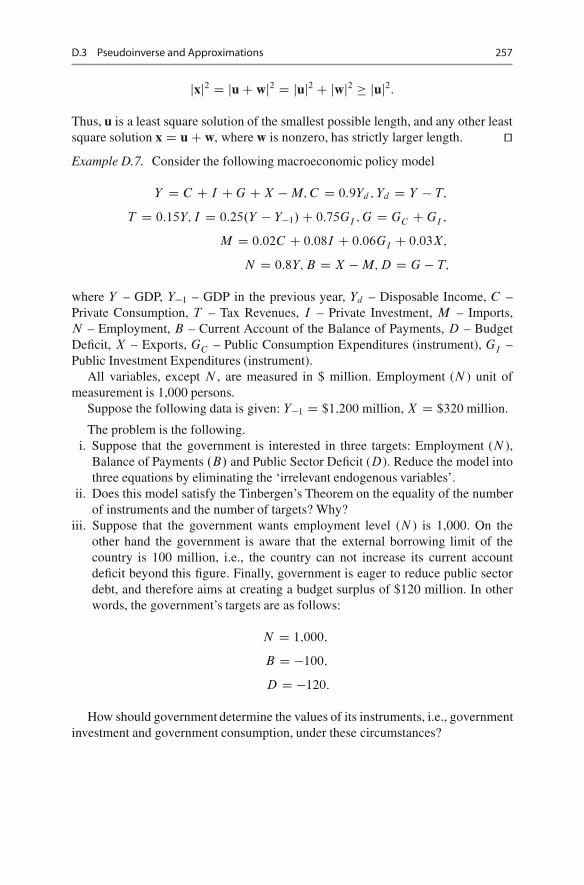
D.3 Pseudoinverse and Approximations 257
jxj2 D juC wj2 D juj2 C jwj2 � juj2:
Thus, u is a least square solution of the smallest possible length, and any other leastsquare solution x D uC w, where w is nonzero, has strictly larger length. utExample D.7. Consider the following macroeconomic policy model
Y D C C I CG CX �M; C D 0:9Yd ; Yd D Y � T;
T D 0:15Y; I D 0:25.Y � Y�1/C 0:75GI ; G D GC CGI ;
M D 0:02C C 0:08I C 0:06GI C 0:03X;
N D 0:8Y; B D X �M; D D G � T;
where Y – GDP, Y�1 – GDP in the previous year, Yd – Disposable Income, C –Private Consumption, T – Tax Revenues, I – Private Investment, M – Imports,N – Employment, B – Current Account of the Balance of Payments, D – BudgetDeficit, X – Exports, GC – Public Consumption Expenditures (instrument), GI –Public Investment Expenditures (instrument).
All variables, except N , are measured in $ million. Employment (N ) unit ofmeasurement is 1,000 persons.
Suppose the following data is given: Y�1 D $1;200 million, X D $320 million.
The problem is the following.i. Suppose that the government is interested in three targets: Employment (N ),
Balance of Payments .B/ and Public Sector Deficit (D). Reduce the model intothree equations by eliminating the ‘irrelevant endogenous variables’.
ii. Does this model satisfy the Tinbergen’s Theorem on the equality of the numberof instruments and the number of targets? Why?
iii. Suppose that the government wants employment level (N ) is 1,000. On theother hand the government is aware that the external borrowing limit of thecountry is 100 million, i.e., the country can not increase its current accountdeficit beyond this figure. Finally, government is eager to reduce public sectordebt, and therefore aims at creating a budget surplus of $120 million. In otherwords, the government’s targets are as follows:
N D 1;000;
B D �100;
D D �120:
How should government determine the values of its instruments, i.e., governmentinvestment and government consumption, under these circumstances?
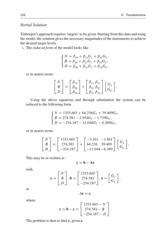
258 D Pseudoinverse
Partial Solution
Tinbergen’s approach requires ‘targets’ to be given. Starting from this data and usingthe model, the solution gives the necessary magnitudes of the instruments to achievethe desired target levels.
i. The reduced form of the model looks like
8<
:
N D ˇ10 C ˇ11GI C ˇ12GC ;
B D ˇ20 C ˇ21GI C ˇ22GC ;
D D ˇ30 C ˇ31GI C ˇ32GC ;
or in matrix terms2
4N
B
D
3
5 D2
4ˇ10
ˇ20
ˇ30
3
5C2
4ˇ11 ˇ12
ˇ21 ˇ22
ˇ31 ˇ32
3
5�
GI
GC
�:
Using the above equations and through substitution the system can bereduced to the following form
8<
:
N D 1355:665C 64:236GI C 39:409GC ;
B D 274:581� 2:954GI � 1:739GC ;
D D �254:187� 11:044GI � 6:389GC ;
or in matrix terms
2
4N
B
D
3
5 D2
41355:665
274:581
�254:187
3
5C2
4�3:161 �1:861
64:236 39:409
�11:044 �6:389
3
5�
GI
GC
�:
This may be re-written asy D b� Ax
with
y D2
4N
B
D
3
5 ; b D2
41355:665
274:581
�254:187
3
5 ; x D�
GI
GC
�;
orAx D c;
where
c D b � y D2
41355:665�N
274:581� B
�254:187�D
3
5 :
The problem is then to find y, given c.
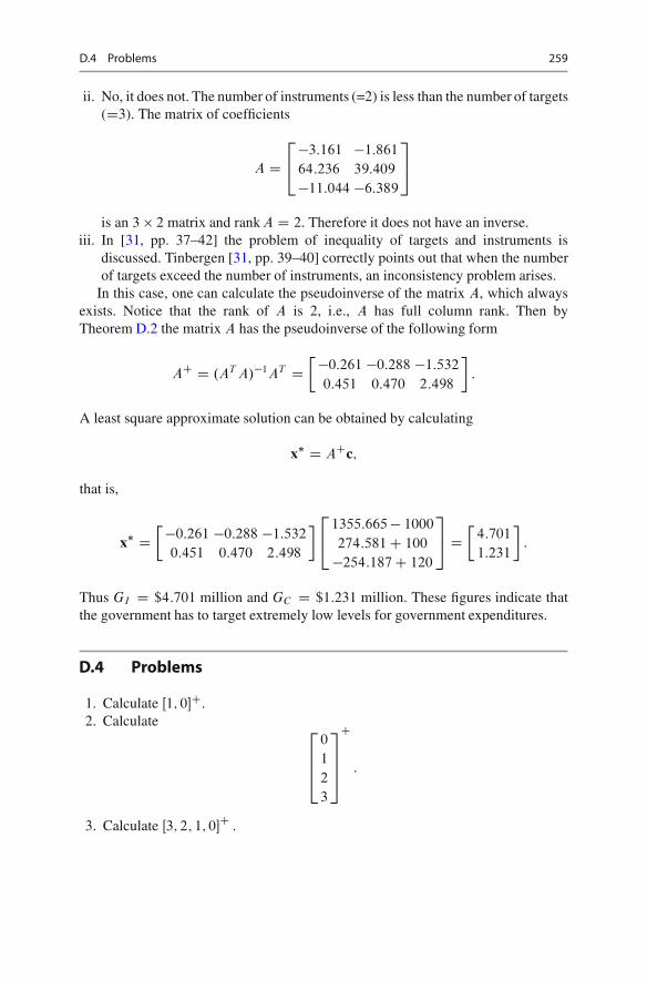
D.4 Problems 259
ii. No, it does not. The number of instruments (=2) is less than the number of targets(D3). The matrix of coefficients
A D2
4�3:161 �1:861
64:236 39:409
�11:044 �6:389
3
5
is an 3 � 2 matrix and rank A D 2. Therefore it does not have an inverse.iii. In [31, pp. 37–42] the problem of inequality of targets and instruments is
discussed. Tinbergen [31, pp. 39–40] correctly points out that when the numberof targets exceed the number of instruments, an inconsistency problem arises.
In this case, one can calculate the pseudoinverse of the matrix A, which alwaysexists. Notice that the rank of A is 2, i.e., A has full column rank. Then byTheorem D.2 the matrix A has the pseudoinverse of the following form
AC D .AT A/�1AT D��0:261 �0:288 �1:532
0:451 0:470 2:498
�:
A least square approximate solution can be obtained by calculating
x� D ACc;
that is,
x� D��0:261 �0:288 �1:532
0:451 0:470 2:498
�2
41355:665� 1000
274:581C 100
�254:187C 120
3
5 D�
4:701
1:231
�:
Thus GI D $4:701 million and GC D $1:231 million. These figures indicate thatthe government has to target extremely low levels for government expenditures.
D.4 Problems
1. Calculate Œ1; 0�C.2. Calculate 2
664
0
1
2
3
3
775
C
:
3. Calculate Œ3; 2; 1; 0�C :
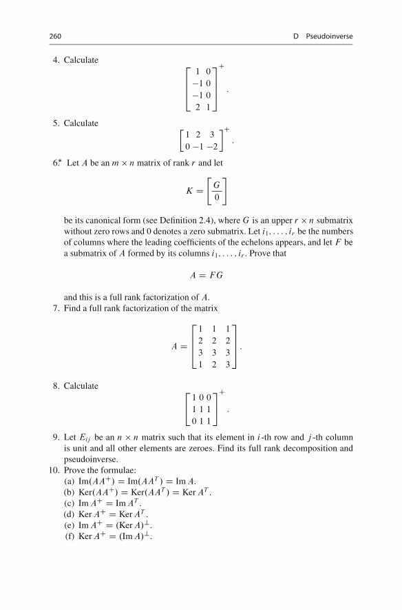
260 D Pseudoinverse
4. Calculate 2
664
1 0
�1 0
�1 0
2 1
3
775
C
:
5. Calculate �1 2 3
0 �1 �2
�C:
6.� Let A be an m � n matrix of rank r and let
K D"
G
0
#
be its canonical form (see Definition 2.4), where G is an upper r � n submatrixwithout zero rows and 0 denotes a zero submatrix. Let i1; : : : ; ir be the numbersof columns where the leading coefficients of the echelons appears, and let F bea submatrix of A formed by its columns i1; : : : ; ir . Prove that
A D F G
and this is a full rank factorization of A.7. Find a full rank factorization of the matrix
A D
2
664
1 1 1
2 2 2
3 3 3
1 2 3
3
775 :
8. Calculate 2
41 0 0
1 1 1
0 1 1
3
5
C
:
9. Let Eij be an n � n matrix such that its element in i -th row and j -th columnis unit and all other elements are zeroes. Find its full rank decomposition andpseudoinverse.
10. Prove the formulae:(a) Im.AAC/ D Im.AAT / D Im A.(b) Ker.AAC/ D Ker.AAT / D Ker AT .(c) Im AC D Im AT .(d) Ker AC D Ker AT .(e) Im AC D .Ker A/?.(f) Ker AC D .Im A/?.

D.4 Problems 261
11. Find the solution of smallest length of the linear system
�2x C 3y C 2z D 7;
3x C 4y � z D 6:
12. Find the least-square solution of smallest length of the linear system
8ˆ<
ˆ:
x � 3y C t D �1;
2y � 3z D �1;
x � 2y C zC t D 0;
x � 2zC t D 8:

•

EAnswers and Solutions
Chapter 1
1. (a)p
137; (b)p
113; (c) 2p
5; 4. (a) y D �2:25x C 1; (b) y D .8=7/x; (c)x D p2. 8. x D 10=7. 10. (a) x D 40=13; y D �15=13; (b)y D 0:6x � 3; (c) nosolutions. 11. z1 D .a11b11 C a12b21/x1 C .a11b12 C a12b22/x2; z2 D .a21b11 Ca22b21/x1 C .a21b12 C a22b22/x2.
Chapter 2
1. (a) x D .3;�1;�3;�3/; (b) x D .�0:2;�0:4;�1/. 4. Yes. 7. (a) 2; (b) 3.
11. 2n. 12. For example, A D B D�
0 1
0 0
�and C D 0. 13. For example,
A D�
1 1
1 1
�; B D
�0 0
0 0
�and C D
�1 1
�1 �1
�. 17. Hint. Use the property
(1-b) of matrix multiplication. 18. For example, A D�
1 0 0
0 1 0
�and B D
2
41 0
0 1
1 1
3
5.
19. (a) x D�
a
a
�for a 2 R; (b) y D �
3b b�
for b 2 R. 22.
2
41 16 0
0 10 0
0 �180 5
3
5.
23. (a) In AB , the i -th and j -th rows are interchanged as well; (b) c times j -th rowof AB will be added to i -th row of AB; (c) i -th and j -th columns of AB are inter-changed as well; (d) c times j -th column of AB will be added to i -th column of AB .
24. Hint. Use Problem 23. 27.�
a b
c �a
�, where bc D �a2. 28. Either A D
�a b
c a
�,
where a2 C bc D 1, or A D ˙I2.
F. Aleskerov et al., Linear Algebra for Economists, Springer Texts in Businessand Economics, DOI 10.1007/978-3-642-20570-5,© Springer-Verlag Berlin Heidelberg 2011
263

264 E Answers and Solutions
29.
2
42 1 �4 5
0 0 1 �3
0 0 0 0
3
5, rank D 2. 30.
2
41 3 0 0
0 0 1 0
0 0 0 1
3
5.
Chapter 3
1. (a) �2; (b) 0; (c) �1; (d) �2b3; (e) sin.˛ � ˇ/; (f) 0. 2. (a) 2; (b) 30; (c) abc C2x3� .aCbCc/x2; (d) ˛2Cˇ2C�2C1; (e) sin.ˇ� �/C sin.��˛/C sin.˛�ˇ/.
3.�
x0y0�D"
1p2
1p2
� 1p2
1p2
#�x
y
��"p
2 � 3p2p
2 � 3p2
#
4. f .A/ D 0. 7. 1875. 8. .�1/nd .
9. (a) 1 for n D 4k and n D 4k C 1, �1 for n D 4k C 2 and n D 4k C 3, where k
is an integer; (b) nC 1; c) 1C .�1/n�12n. 10. det X D 1. Solution. We have
X3 � In D .X � In/.X2 CX C In/ D .X � In/0 D 0;
hence X3 D In. Then det.X3/ D det In D 1, that is, .det X/3 D 1 and det X D 1.
Chapter 4
1. (a)
��2 1
1:5 �0:5
�; (b)
�cos ˛ sin ˛
� sin ˛ cos ˛
�; (c)
2
4�7=3 2 �1=3
5=3 �1 �1=3
�2 1 1
3
5;
(d) 19�2
41 2 2
2 1 �2
2 �2 1
3
5; (e)
2
664
�1 1 16 �9
�8 7 125 �70
�10 9 160 �90
�1 1 18 �10
3
775. 2. (a)
2
666664
1 �1 0 : : : 0
0 1 �1 : : : 0
0 0 1 : : : 0:::
::::::
: : ::::
0 0 0 : : : 1
3
777775
;
(b)
2
666664
2 � n 1 1 : : : 1
1 �1 0 : : : 0
1 0 �1 : : : 0:::
::::::
: : ::::
1 0 0 : : : �1
3
777775
; (c) 1n�1
2
666664
2 � n 1 1 : : : 1
1 2 � n 1 : : : 1
1 1 2 � n : : : 1:::
::::::
: : ::::
1 1 1 : : : 2 � n
3
777775
.
3. (a)
��1 a � 10
2 7:5 � 0:5a
�; (b)
�10:5 6:5
11 �7
�; (c)
2
41 2 3
4 5 6
7 8 9
3
5; (d)
2
41 1 1
1 2 3
2 3 1
3
5.
7. (a) 3; (b) 3 for � D ˙1, 4 for � ¤ ˙1. 9. rank
�x2 � x1 x3 � x1
y2 � y1 y3 � y1
�� 1.
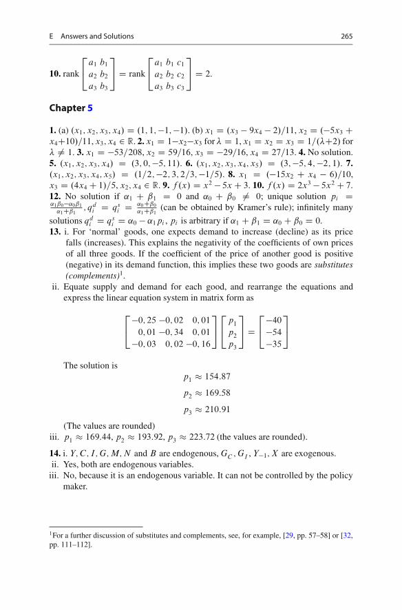
E Answers and Solutions 265
10. rank
2
4a1 b1
a2 b2
a3 b3
3
5 D rank
2
4a1 b1 c1
a2 b2 c2
a3 b3 c3
3
5 D 2.
Chapter 5
1. (a) .x1; x2; x3; x4/ D .1; 1;�1;�1/. (b) x1 D .x3 � 9x4 � 2/=11, x2 D .�5x3 Cx4C10/=11, x3; x4 2 R. 2. x1 D 1�x2�x3 for � D 1, x1 D x2 D x3 D 1=.�C2/ for� ¤ 1. 3. x1 D �53=208, x2 D 59=16, x3 D �29=16, x4 D 27=13. 4. No solution.5. .x1; x2; x3; x4/ D .3; 0;�5; 11/. 6. .x1; x2; x3; x4; x5/ D .3;�5; 4;�2; 1/. 7..x1; x2; x3; x4; x5/ D .1=2;�2; 3; 2=3;�1=5/. 8. x1 D .�15x2 C x4 � 6/=10,x3 D .4x4C 1/=5, x2; x4 2 R. 9. f .x/ D x2 � 5xC 3. 10. f .x/ D 2x3 � 5x2C 7.12. No solution if ˛1 C ˇ1 D 0 and ˛0 C ˇ0 ¤ 0; unique solution pi D˛1ˇ0�˛0ˇ1
˛1Cˇ1; qd
i D qsi D ˛0Cˇ0
˛1Cˇ1(can be obtained by Kramer’s rule); infinitely many
solutions qdi D qs
i D ˛0 � ˛1pi , pi is arbitrary if ˛1 C ˇ1 D ˛0 C ˇ0 D 0.13. i. For ‘normal’ goods, one expects demand to increase (decline) as its price
falls (increases). This explains the negativity of the coefficients of own pricesof all three goods. If the coefficient of the price of another good is positive(negative) in its demand function, this implies these two goods are substitutes(complements)1.
ii. Equate supply and demand for each good, and rearrange the equations andexpress the linear equation system in matrix form as
2
4�0; 25 �0; 02 0; 01
0; 01 �0; 34 0; 01
�0; 03 0; 02 �0; 16
3
5
2
4p1
p2
p3
3
5 D2
4�40
�54
�35
3
5
The solution isp1 154:87
p2 169:58
p3 210:91
(The values are rounded)iii. p1 169:44, p2 193:92, p3 223:72 (the values are rounded).
14. i. Y; C; I; G; M; N and B are endogenous, GC ; GI , Y�1; X are exogenous.ii. Yes, both are endogenous variables.
iii. No, because it is an endogenous variable. It can not be controlled by the policymaker.
1For a further discussion of substitutes and complements, see, for example, [29, pp. 57–58] or [32,pp. 111–112].
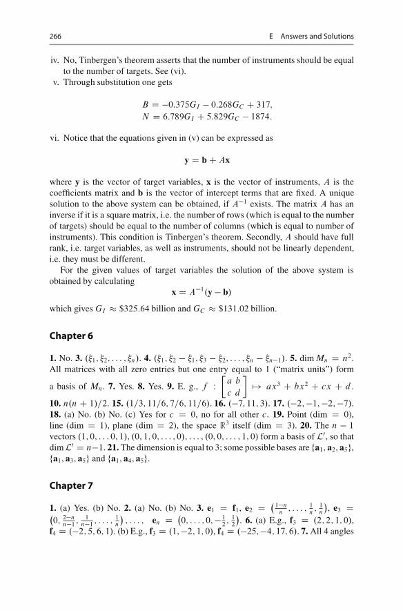
266 E Answers and Solutions
iv. No, Tinbergen’s theorem asserts that the number of instruments should be equalto the number of targets. See (vi).
v. Through substitution one gets
B D �0:375GI � 0:268GC C 317;
N D 6:789GI C 5:829GC � 1874:
vi. Notice that the equations given in (v) can be expressed as
y D bC Ax
where y is the vector of target variables, x is the vector of instruments, A is thecoefficients matrix and b is the vector of intercept terms that are fixed. A uniquesolution to the above system can be obtained, if A�1 exists. The matrix A has aninverse if it is a square matrix, i.e. the number of rows (which is equal to the numberof targets) should be equal to the number of columns (which is equal to number ofinstruments). This condition is Tinbergen’s theorem. Secondly, A should have fullrank, i.e. target variables, as well as instruments, should not be linearly dependent,i.e. they must be different.
For the given values of target variables the solution of the above system isobtained by calculating
x D A�1.y � b/
which gives GI $325:64 billion and GC $131:02 billion.
Chapter 6
1. No. 3. .�1; �2; : : : ; �n/. 4. .�1; �2 � �1; �3 � �2; : : : ; �n � �n�1/. 5. dim Mn D n2.All matrices with all zero entries but one entry equal to 1 (“matrix units”) form
a basis of Mn. 7. Yes. 8. Yes. 9. E. g., f W�
a b
c d
�7! ax3 C bx2 C cx C d .
10. n.n C 1/=2. 15. .1=3; 11=6; 7=6; 11=6/. 16. .�7; 11; 3/. 17. .�2;�1;�2;�7/.18. (a) No. (b) No. (c) Yes for c D 0, no for all other c. 19. Point (dim D 0),line (dim D 1), plane (dim D 2), the space R3 itself (dim D 3). 20. The n � 1
vectors .1; 0; : : : 0; 1/; .0; 1; 0; : : : ; 0/; : : : ; .0; 0; : : : ; 1; 0/ form a basis of L0, so thatdimL0 D n�1. 21. The dimension is equal to 3; some possible bases are fa1; a2; a5g,fa1; a3; a5g and fa1; a4; a5g.
Chapter 7
1. (a) Yes. (b) No. 2. (a) No. (b) No. 3. e1 D f1, e2 D
1�nn
; : : : ; 1n; 1
n
, e3 D
0; 2�nn�1
; 1n�1
; : : : ; 1n
; : : : ; en D
0; : : : ; 0;� 1
2; 1
2
. 6. (a) E.g., f3 D .2; 2; 1; 0/,
f4 D .�2; 5; 6; 1/. (b) E.g., f3 D .1;�2; 1; 0/, f4 D .�25;�4; 17; 6/. 7. All 4 angles
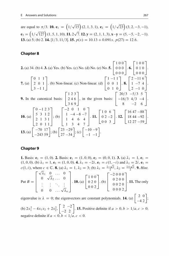
E Answers and Solutions 267
are equal to �=3. 10. e1 D�1=p
15�
.2; 1; 3; 1/, e2 D�1=p
23�
.3; 2;�3;�1/,
e3 D�1=p
127�
.1; 5; 1; 10/. 11. 2p
7. 12. y D .2; 1; 1; 3/, x�y D .5;�5;�2;�1/.
13. (a) 5; (b) 2. 14. Œ1=3; 11=3�. 15. p.x/ D 10:13C 0:091x; p.27/ D 12:6.
Chapter 8
2. (a) 34. (b) 4. 3. (a) Yes. (b) Yes. (c) No. (d) No. (e) No. 5.
2
41 0 0
0 0 0
0 0 0
3
5. 6.
2
41 0 0
0 1 0
0 0 0
3
5.
7. (a)
2
40 1 1
2 0 1
3 �1 1
3
5. (b) Non-linear. (c) Non-linear. (d)
2
41 �1 1
0 0 1
0 1 0
3
5. 8.
2
42 �11 6
1 �7 4
2 �1 0
3
5.
9. In the canonical basis:
2
41 2 3
2 4 6
3 6 9
3
5, in the given basis:
2
420=3 �5=3 5
�16=3 4=3 �4
8 �2 6
3
5.
10. (a)
2
664
0 �1 2 3
5 3 1 2
2 1 3 1
2 0 1 1
3
775; (b)
2
664
�2 0 1 0
1 �4 �8 �7
1 4 6 4
1 3 4 7
3
775. 11.
2
41 0 6
0 2 �2
0 0 3
3
5. 12.
2
416 47 �88
18 44 �92
12 27 �59
3
5.
13. (a)
� �70 17
�243 59
�; (b)
�23 �29
27 �34
�; (c)
��10 �9
�1 �1
�.
Chapter 9
1. Basis: e1 D .1; 0/. 2. Basis: e1 D .1; 0; 0/, e2 D .0; 0; 1/. 3. (a) �1 D 1, e1 D.1; 0; 0/. (b) �1 D 1, e1 D .1; 0; 0/. 4. �1 D �2i , e1 D c.1;�i/ and �1 D 2i , e1 Dc.1; i/, where c 2 C. 8. (a) �1 D 1, �2 D 3; (b) �1 D 1�p
52
, �2 D 1Cp5
2. 9. Hint.
Put B D
2
6664
p�1 0 : : : 0
0p
�2 : : : 0:::
:::: : :
:::
0 0 : : :p
�n
3
7775
: 10. (a)
2
41 0 0
0 2 0
0 0 2
3
5. (b)
2
664
�2 0 0 0
0 2 0 0
0 0 2 0
0 0 0 2
3
775. 11. The only
eigenvalue is � D 0; the eigenvectors are constant polynomials. 14. (a)
�2 0
�4 2
�;
(b) 2x21 � 4x1x2 C 2x2
2 ,
�2 �2
�2 2
�. 15. Positive definite if a > 0; b > 1=a; c > 0;
negative definite if a < 0; b < 1=a; c < 0.
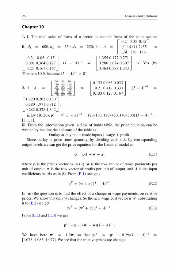
268 E Answers and Solutions
Chapter 10
1. i. The total sales of firms of a sector to another firms of the same sector;
ii. d1 D 600; d2 D 230; d3 D 250; iii. A D2
40:2 0:05 0:15
1=11 4=11 7=55
1=4 1=6 1=6
3
5 2
40:2 0:05 0:15
0:091 0:364 0:127
0:25 0:167 0:167
3
5, .I � A/�1 D2
41:355 0:177 0:271
0:286 1:674 0:307
0:464 0:388 1:343
3
5; iv. Yes (by
Theorem 10.9, because .I � A/�1 > 0).
2. i. A D2
420150
40480
10300
30150
200480
100300
20150
60480
50300
3
5 2
40:133 0:083 0:033
0:2 0:417 0:333
0:133 0:125 0:167
3
5 ; .I � A/�1 2
41:220 0:202 0:130
0:580 1:971 0:812
0:282 0:328 1:342
3
5 :
ii. By (10.26), pT D vT .I �A/�1 D .80=150; 180=480; 140=300/ .I � A/�1 DŒ1; 1; 1�:
iii. From the information given in flow of funds table, the price equation can bewritten by reading the columns of the table as
OutlayD payments made inputsC wageC profit.Since outlay is price times quantity, by dividing each side by corresponding
output levels we can get the price equation for the Leontief model as
p D pAC wC �; (E.1)
where p is the prices vector as in (ii), w is the row vector of wage payments perunit of output, � is the row vector of profits per unit of output, and A is the inputcoefficients matrix as in (i). From (E.1) one gets
pT D .wC �/.I � A/�1: (E.2)
In (iii) the question is to find the effect of a change in wage payments, on relativeprices. We know that only w changes. So the new wage cost vector is w0, substitutingit to (E.2) we get
p0T D .w0 C �/.I � A/�1: (E.3)
From (E.2) and (E.3) we get
p0T � p D .w0 � w/.I � A/�1:
We have here w0 D 1:2w, so that p0T D pT C 0:2w.I � A/�1 Œ1:078; 1:085; 1:077�. We see that the relative prices are changed.
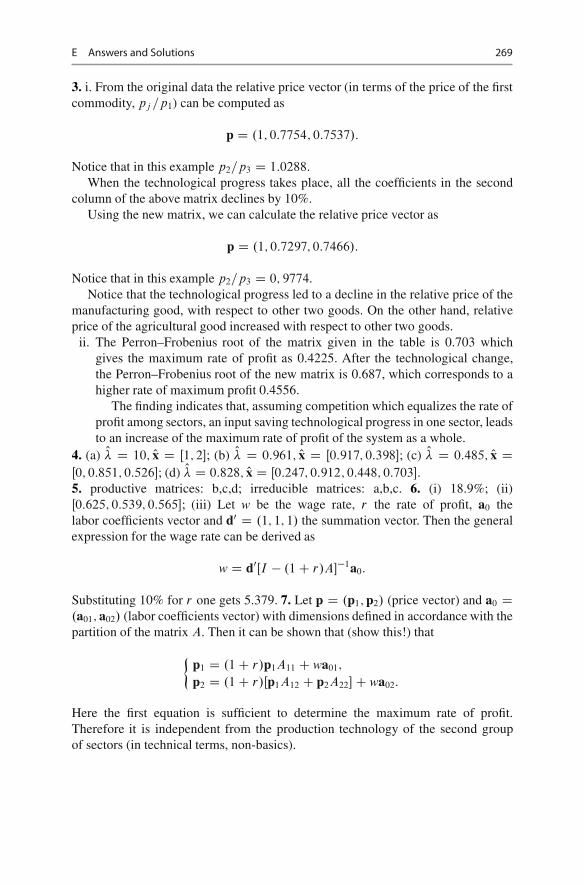
E Answers and Solutions 269
3. i. From the original data the relative price vector (in terms of the price of the firstcommodity, pj =p1) can be computed as
p D .1; 0:7754; 0:7537/:
Notice that in this example p2=p3 D 1:0288.When the technological progress takes place, all the coefficients in the second
column of the above matrix declines by 10%.Using the new matrix, we can calculate the relative price vector as
p D .1; 0:7297; 0:7466/:
Notice that in this example p2=p3 D 0; 9774.Notice that the technological progress led to a decline in the relative price of the
manufacturing good, with respect to other two goods. On the other hand, relativeprice of the agricultural good increased with respect to other two goods.
ii. The Perron–Frobenius root of the matrix given in the table is 0.703 whichgives the maximum rate of profit as 0.4225. After the technological change,the Perron–Frobenius root of the new matrix is 0.687, which corresponds to ahigher rate of maximum profit 0.4556.
The finding indicates that, assuming competition which equalizes the rate ofprofit among sectors, an input saving technological progress in one sector, leadsto an increase of the maximum rate of profit of the system as a whole.
4. (a) O� D 10; Ox D Œ1; 2�; (b) O� D 0:961; Ox D Œ0:917; 0:398�; (c) O� D 0:485; Ox DŒ0; 0:851; 0:526�; (d) O� D 0:828; Ox D Œ0:247; 0:912; 0:448; 0:703�.5. productive matrices: b,c,d; irreducible matrices: a,b,c. 6. (i) 18.9%; (ii)Œ0:625; 0:539; 0:565�; (iii) Let w be the wage rate, r the rate of profit, a0 thelabor coefficients vector and d0 D .1; 1; 1/ the summation vector. Then the generalexpression for the wage rate can be derived as
w D d0ŒI � .1C r/A��1a0:
Substituting 10% for r one gets 5.379. 7. Let p D .p1; p2/ (price vector) and a0 D.a01; a02/ (labor coefficients vector) with dimensions defined in accordance with thepartition of the matrix A. Then it can be shown that (show this!) that
�p1 D .1C r/p1A11 C wa01;
p2 D .1C r/Œp1A12 C p2A22�C wa02:
Here the first equation is sufficient to determine the maximum rate of profit.Therefore it is independent from the production technology of the second groupof sectors (in technical terms, non-basics).

270 E Answers and Solutions
Chapter 11
6. (a) Square with vertices .0; 2/; .�2; 0/; .0;�2/; .2; 0/; (b) square with vertices.2; 2/; .�2; 2/; .�2;�2/; .2;�2/. 7. (a) Yes; (b) Yes; (c) Yes. 8. (a) H ŒC�; (b) H Œ��;(c) H . 10. Not necessary. For example, the union of two lines l1 W y D 0 andl2 W x D 0 in R2 is not convex. 11. Hint. The problem can be posed in the followingway:
maxx1;x2
75x1 C 55x2
under the conditions 8ˆ<
ˆ:
x1 C x2 � 100;
7x1 C 5x2 � 1000;
2x1 C 3x2 � 150;
x1; x2 � 0;
where x1 acres of land should be allocated to wheat and x2 acres of land should beallocated to barley.Answer. x1 D 50; x2 D 0. Net revenue will be $450.
12. Hint. Let X1 be the amount invested in government bonds, X2 the amountinvested in auto company A, X3 the amount invested in auto company B, X4
the amount invested in textile company C, and X5 the amount invested in textilecompany D.
Then the objective function is
max 0:035X1 C 0:055X2 C 0:065X3 C 0:06X4 C 0:09X5
with the constrains8ˆˆ<
ˆˆ:
X1 CX2 CX3 CX4 CX5 D 1000000;
X2 CX3 � 500000;
X4 CX5 � 500000;
X1 � 0:35.X2 CX3/ � 0;
X5 � 0:65.X4 CX5/ � 0
andX1; X2; X3; X4; X5 � 0:
Answer. Projected return (value of the objective function): $68, 361, X1 D 129; 630,X2 D 0, X3 D 370;370, X4 D 175; 000, X5 D 325; 000. Thus the LP solutionsuggests that the portfolio manager should not invest in auto company A.
13. Hint. The problem can be formulated as follows.The objective is to minimize risk under the conditions given above.Objective function: min 4x C 9y.Fund availability constraint: 50x C 150y � 10;000;000.
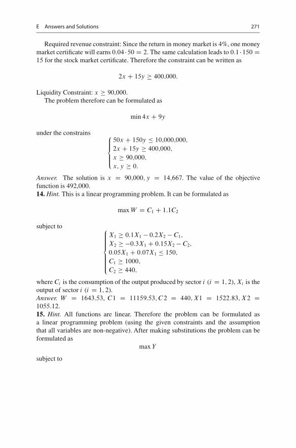
E Answers and Solutions 271
Required revenue constraint: Since the return in money market is 4%, one moneymarket certificate will earns 0:04 �50 D 2. The same calculation leads to 0:1 �150 D15 for the stock market certificate. Therefore the constraint can be written as
2x C 15y � 400;000:
Liquidity Constraint: x � 90;000.The problem therefore can be formulated as
min 4x C 9y
under the constrains 8ˆ<
ˆ:
50x C 150y � 10;000;000;
2x C 15y � 400;000;
x � 90;000;
x; y � 0:
Answer. The solution is x D 90;000; y D 14;667: The value of the objectivefunction is 492,000.14. Hint. This is a linear programming problem. It can be formulated as
max W D C1 C 1:1C2
subject to 8ˆˆ<
ˆˆ:
X1 � 0:1X1 � 0:2X2 � C1;
X2 � �0:3X1 C 0:15X2 � C2;
0:05X1 C 0:07X1 � 150;
C1 � 1000;
C2 � 440;
where Ci is the consumption of the output produced by sector i (i D 1; 2), Xi is theoutput of sector i (i D 1; 2).Answer. W D 1643:53, C1 D 11159:53; C 2 D 440; X1 D 1522:83; X2 D1055:12.15. Hint. All functions are linear. Therefore the problem can be formulated asa linear programming problem (using the given constraints and the assumptionthat all variables are non-negative). After making substitutions the problem can beformulated as
max Y
subject to
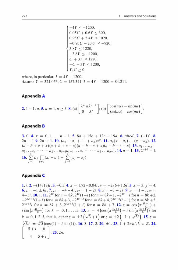
272 E Answers and Solutions
8ˆˆˆˆˆˆ<
ˆˆˆˆˆˆ:
�4Y � �1200;
0:05C C 0:6Y � 300;
0:95C C 2:4Y � 1020;
�0:95C � 2:4Y � �920;
3:8Y � 1220;
�3:8Y � �1200;
C C 3Y � 1220;
�C � 3Y � 1200;
Y; C � 0;
where, in particular, I D 4Y � 1200.Answer. Y D 321:053; C D 157:341; I D 4Y � 1200 D 84:211:
Appendix A
2. 1 � 1=n. 5. n D 1; n � 5. 8. (a)
��n n�n�1
0 �n
�; (b)
�cos.n˛/ � sin.n˛/
sin.n˛/ cos.n˛/
�.
Appendix B
3. 0. 4. x D 0; 1; : : : ; n � 1. 5. 8a C 15b C 12c � 19d . 6. abcd . 7. .�1/n. 8.2n C 1 9. 2n C 1. 10. .a0 C a1 C � � � C an/xn. 11. a0.x � a1/ : : : .x � an/. 12..a � b C c C x/.a C b C c � x/.a C b � c C x/.a � b � c � x/. 13. a1 : : : an �a3 : : : an � � � � � a2 : : : ai�1aiC1 : : : an � � � � � a2 : : : an�1. 14. nC 1. 15. 2nC1 � 1.
16.nP
j D1
aj
Q
i¤j
.xi � ai /CnP
j D1
.xj � aj /
Appendix C
1. i . 2.�.14=13/i . 3.�0:5. 4. x D 1:72�0:04i; y D �2=6C1:6i . 5. x D 3; y D 4.6. z D �1˙ 6i . 7. z1 D �4� 4i; z2 D 1C 2i . 8. z D �3C 2i . 9. z1 D 1C i; z2 D4�5i . 10. 1. 11. 24k for n D 8k, 24k.1�i/ for n D 8kC1,�24kC1i for n D 8kC2,�24kC1.1Ci/ for n D 8kC3,�24kC2 for n D 8kC4, 24kC2.i�1/ for n D 8kC5,24kC3i for n D 8k C 6, 24kC3.1 C i/ for n D 8k C 7. 12. z D cos
� 4kC1
12
Ci sin
� 4kC1
12
for k D 0; 1; : : : ; 5. 13. z D 4
cos
� 3kC1
6
C i sin� 3kC1
6
for
k D 0; 1; 2; 3, that is, either z D ˙2�p
3C i�
or z D ˙2��1Cp3i
�. 15. z D
5p
5ei D 5p
5 .cos .1/C i sin .1//. 16. 3. 17. 2. 20. ˙1. 23. 1 C 2�ki; k 2 Z. 24."�5C i �6
4 5C i
#
: 25. 2n.
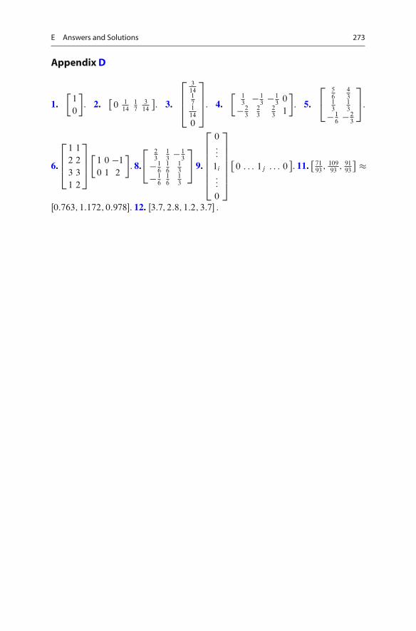
E Answers and Solutions 273
Appendix D
1.�
1
0
�. 2.
�0 1
1417
314
�. 3.
2
664
31417114
0
3
775. 4.
�13� 1
3� 1
30
� 23
23
23
1
�. 5.
2
456
43
13
13
� 16� 2
3
3
5.
6.
2
664
1 1
2 2
3 3
1 2
3
775
�1 0 �1
0 1 2
�. 8.
2
423
13� 1
3
� 16
16
13
� 16
16
13
3
5 9.
2
6666664
0:::
1i
:::
0
3
7777775
�0 : : : 1j : : : 0
�. 11.
�7193
; 10993
; 9193
�
Œ0:763; 1:172; 0:978�. 12. Œ3:7; 2:8; 1:2; 3:7� :

•

References
1. Abadir, K.M., Magnus, J.R.: Matrix Algebra, Econometric Exercises Series, No. 1. CambridgeUniversity Press, Cambridge (2005)
2. Ben-Israel, A., Greville, T.: Generalized Inverses. Theory and Applications, 2nd edn. Springer,New York (2003)
3. Bapat, R.B., Raghavan, T.E.S.: Nonnegative Matrices And Applications. Cambridge UniversityPress, Cambridge (1997)
4. Braverman, E.M.: Mathematical Models of Planning and Control in Economic Systems.Nauka, Moscow [in Russian] (1976)
5. Campbell, S.L., Meyer, C.D., Jr.: Generalized Inverses of Linear Transformations. Dover,New York (1991)
6. Dasgupta, D.: Using the correct economic interpretation to prove the Hawkins-Simon-Nikaidotheorem: One more now. J. Macroecon. 14(4), 755–761 (1992)
7. Debreu, G., Herstein, I.N.: Nonnegative square matrices. Econometrica 21, 597–607 (1953)(see also in [20, pp. 57–67])
8. Dhrymes, P.J.: Mathematics for Econometrics, 3rd edn. Springer, New York (2000)9. Diewert, E.: Index numbers. In: Durlauf, S.N., Blume, L.E. (eds.) The New Palgrave Dictionary
of Economics, 2nd edn. Palgrave Macmillan, New York (2008)10. Gantmacher, F.R.: Theory of Matrices, Vols. 1, 2. Chelsea Publishing, New York (1959)11. Gel’fand, I.M.: Lectures on Linear Algebra (with the collaboration of Z. Ya. Shapiro), Dover
Books on Advanced Mathematics. Dover Publications, New York (1989)12. Hawkins, D., Simon, H.A.: Note: some conditions of macroeconomic stability. Econometrica
17, 245–248 (1949)13. Hawkins, Th.: Continued fractions and the origins of the Perron–Frobenius theorem. Archive
History Exact Sci. 62(6), 655–717 (2008)14. Judge, G.G., Griffiths, W.E., Hill, R.C., Lutkepohl, H., Lee, T.-C.: The Theory and Practice of
Econometrics, 2nd edn. Wiley, New York (1985)15. Krattenthaler, C.: Advanced Determinant Calculus, The Andrews Festschrift (Maratea, 1998).
Sem. Lothar. Combin. 42, Art. B42q, 67 pp. (electronic) (1999)16. Kurz, M.D., Salvatori, N.: Theory of Production. Cambridge University Press, Cambridge
(1995)17. Kurz, M.D., Salvadori, N.: “Classical” roots of input–output analysis: a short account of its
long history. Econ. Syst. Res. XII, 153–179 (2000)18. Kurz, M.D., Salvadori, N.: Input–output analysis from a wider perspective: a comparison of
the early works of Leontief and Sraffa. Econ. Syst. Res. 18(4), 373–390 (2006)19. Lang, S.: Linear Algebra, Undergraduate Texts in Mathematics. Springer, New York (1989)
F. Aleskerov et al., Linear Algebra for Economists, Springer Texts in Businessand Economics, DOI 10.1007/978-3-642-20570-5,© Springer-Verlag Berlin Heidelberg 2011
275

276 References
20. Newman, P.: Readings in Mathematical Economics-I, Value Theory. The Johns Hopkins Press,Baltimore (1968)
21. O’Neill, M.J., Wood, R.J.: An Alternative Proof of the Hawkins-Simon Condition. Asia-PacificJ. Oper. Res. 16(2), 173–184 (1999)
22. Pasinetti, L.: Lectures on the Theory of Production. Columbia University Press, New York(1977)
23. Persky, J.: Price indexes and general exchange values. J. Econ. Perspect. 12(1), 197–205 (1998)24. Prasolov, V.V.: Problems and Theorems in Linear algebra, Translations of Mathematical
Monographs, vol. 134. American Mathematical Society, Providence, RI (1994)25. Proskuryakov I.V.: Problems in Linear Algebra. Mir, Moscow (1978)26. Searle, S.R., Willett, L.S.: Matrix Algebra for Applied Economics. Wiley, New York (2001)27. Shilov, G.E.: Linear Algebra. Dover Publications, New York (1977)28. Sraffa, P.: Production of Commodities by Means of Commodities-Prelude to a Critique of
Economic Theory. Cambridge University Press, Cambridge (1960)29. Stiglitz, J.E., Walsh, C.E.: Economics, 4th edn. W.W. Norton, New York (2006)30. Takayama, A.: Mathematical Economics, 2nd edn. Cambridge University Press, Cambridge
(1985)31. Tinbergen, J.: On The Theory of Economic Policy. North Holland, Amsterdam (1952)32. Varian, H.R.: Intermediate Microeconomics – A Modern Approach, 6th edn. W.W. Norton,
New York (2003)33. Vinberg, E.B.: A Course in Algebra, Graduate Studies in Mathematics, vol. 56. American
Mathematical Society, Providence, RI (2003)34. Yaari, M.E.: Linear Algebra for Social Sciences. Prentice-Hall, Englewood Cliffs, New Jersey
(1971)
Index
Adjoint matrix, 67Argument of a complex number, 239
Basic commodity, 187, 189Basis, 95
canonical for Rn, 95orthogonal, 109orthonormal, 109
Basis transformation matrix, 100Bilinear form, 157
symmetric, 157
Canonical basis for Rn, 95Canonical form (of a matrix), 42Cauchy inequality, 26Characteristic polynomial, 145Closed half-space, 204Cofactor, 55Collinear vectors, 95Commodity
basic, 187, 189Complex multiplication, 237Complex number, 237Complex vector space, 244Complexification, 245Component of a vector, 17Condition
Hawkins–Simon, 176Constant returns to scale technology, 104Convex set, 200coordinates, 96
Decreasing returns to scale, 104Determinant, 55
Dimension of a linear space, 92Direct product of matrices, 34Distance
between a vector and a subspace, 115between two vectors, 108
Dot product, 23, 107
Eigenvalue, 142Perron–Frobenius, 185
Eigenvector, 142Perron–Frobenius, 185
Elementary operations of matrices, 38Elementwise product of matrices, 35Exponent of a complex number, 241
Full image, 123Full rank, 71Full rank factorization, 253Fundamental theorem of algebra, 242
Gaussian elimination procedure, 42, 43Gram–Schmidt orthogonalization process, 112
Hadamard product of matrices, 35Half-space
closed, 204open, 204
Hawkins–Simon condition, 176Hawkins–Simon theorem, 176Homogeneous system of linear equations, 37Homomorphism, 123Hypercube, 206Hyperplane, 100, 202
F. Aleskerov et al., Linear Algebra for Economists, Springer Texts in Businessand Economics, DOI 10.1007/978-3-642-20570-5,© Springer-Verlag Berlin Heidelberg 2011
277

278 Index
Identical operator, 125Identity matrix, 31, 51Image, 123, 133
full, 123Imaginary axis, 237Imaginary part of a complex number, 237Imaginary unit, 237Inconsistent system of linear equations, 81Increasing returns to scale, 104Indecomposable matrix, 178Induction, 217Induction assumption, 219Induction principle, 219Induction variable, 219Inner product, 23, 107Invariant subspace, 141Inverse of a mapping, 123Inverse of a matrix, 65Inverse of an operator, 132Irreducible matrix, 178Isomorphic linear spaces, 97
Kernel, 134Kronecker delta function, 51Kronecker product of matrices, 34Kronecker–Capelli theorem, 76
Leading coefficient (of a row of a matrix), 42Leontief model, 172Linear combination, 92Linear mapping, 123Linear operator, 124Linear programming problem, 195Linear space, 91
dimension of, 92Linear spaces
isomorphic, 97Linear transformation, 124Linearly dependent vectors, 20, 92Linearly independent vectors, 21, 92Lower triangular matrix, 56
Mapping, 123Mathematical induction, 219Matrices
similar, 136Matrix, 30
symmetric, 36transpose of, 35adjoint, 67basis transformation, 100
canonical form of, 42elementary operations, 38full rank factorization of, 253identity, 31, 51indecomposable, 178inverse, 65irreducible, 178lower triangular, 56modal, 155nilpotent, 73non-negative, 31null, 31of a full rank, 71of a linear transformation, 126order, 31polynomial of, 52positive, 31power of, 52productive, 172rank, 38reducible, 177row echelon form of, 42singular, 67upper triangular, 56
Minor, 55Modal matrix, 155Multiplication
complex, 237Multiplicity of a root, 243
Natural numbers, 217Nilpotent matrix, 73Non-collinear vectors, 95Non-negative matrix, 31Non-negative vector, 18Non-singular orthogonal operator, 153Null matrix, 31Null operator, 125Null vector, 18Numeraire, 182Number
complex, 237pure imaginary, 237
Open half-space, 204Operator, 124
identical, 125linear, 124null, 125orthogonal, 153orthogonal non-singular, 153orthogonal singular, 153self-adjoint, 150
Index 279
Order of the matrix, 31Orthogonal basis, 109Orthogonal operator, 153Orthonormal basis, 109Oversized enterprise, 104
Peano axioms, 218Perron–Frobenius eigenvalue, 185Perron–Frobenius eigenvector, 185Polynomial of a matrix, 52Polytope, 204Positive matrix, 31Positive vector, 18Power of a matrix, 52Product of matrices, 32
direct, 34elementwise, 35Frobenius, 46Hadamard, 35Kronecker, 34Shur, 35tensor, 34
Productive matrix, 172Productive system, 172Projection of a vector to a subspace, 114Projection of a vector to a unit vector, 113Pseudoinverse, 250Pure imaginary number, 237
Quadratic form, 157
Rank of a matrix, 38Real axis, 237Real part of a complex number, 237Real space, 17Real vector space, 244Reducible matrix, 177Root
simple, 243Rotation matrix, 33Row echelon form (of a matrix), 42
Scalar, 17Scalar product, 23, 107Self-adjoint operator, 150Set
convex, 200Shur product of matrices, 35
Similar matrices, 136Simple root, 243Singular matrix, 67Singular orthogonal operator, 153Span, 99Sraffa Model, 183Strongest Induction Principle, 222Subspace, 98
invariant, 141spanned by given vectors, 99
Sylvester criterion, 159Symmetric matrix, 36System
productive, 172System of linear equations
homogeneous, 37inconsistent, 81
Tensor product of matrices, 34Theorem
Hawkins–Simon, 176Trace of a matrix, 35Transformation, 124
linear, 124Translation, 124Transpose of a matrix, 35
Upper triangular matrix, 56
Vandermonde determinant, 232Vector, 17, 91
components, 17non-negative, 18positive, 18projection of, 113, 114
Vector space, 91Vector space over complex numbers, 244Vector space over real numbers, 244Vectors
collinear, 95linearly dependent, 20, 92linearly independent, 21, 92non-collinear, 95orthogonal, 25parallel, 27
Vertex of a polytope, 205
Zero vector, 18