Linear Algebra Essentials
59
Chapter 2 Linear Algebra Essentials When elementary school students first leave the solid ground of arithmetic for the more abstract world of algebra, the first objects they encounter are generally linear expressions. Algebraically, linear equations can be solved using elementary field properties, namely the existence of additive and multiplicative inverses. Geometrically, a nonvertical line in the plane through the origin can be described completely by one number—the slope. Linear functions f : R → R enjoy other nice properties: They are (in general) invertible, and the composition of linear functions is again linear. Yet marching through the progression of more complicated functions and ex- pressions—polynomial, algebraic, transcendental—many of these basic properties of linearity can become taken for granted. In the standard calculus sequence, sophisticated techniques are developed that seem to yield little new information about linear functions. Linear algebra is generally introduced after the basic calculus sequence has been nearly completed, and is presented in a self-contained manner, with little reference to what has been seen before. A fundamental insight is lost or obscured: that differential calculus is the study of nonlinear phenomena by “linearization.” The main goal of this chapter is to present the basic elements of linear algebra needed to understand this insight of differential calculus. We also present some geometric applications of linear algebra with an eye toward later constructions in differential geometry. While this chapter is written for readers who have already been exposed to a first course in linear algebra, it is self-contained enough that the only essential prerequisites will be a working knowledge of matrix algebra, Gaussian elimination, and determinants. A. McInerney, First Steps in Differential Geometry: Riemannian, Contact, Symplectic, Undergraduate Texts in Mathematics, DOI 10.1007/978-1-4614-7732-7 2, © Springer Science+Business Media New York 2013 9
Transcript of Linear Algebra Essentials

Chapter 2Linear Algebra Essentials
When elementary school students first leave the solid ground of arithmetic forthe more abstract world of algebra, the first objects they encounter are generallylinear expressions. Algebraically, linear equations can be solved using elementaryfield properties, namely the existence of additive and multiplicative inverses.Geometrically, a nonvertical line in the plane through the origin can be describedcompletely by one number—the slope. Linear functions f : R → R enjoy othernice properties: They are (in general) invertible, and the composition of linearfunctions is again linear.
Yet marching through the progression of more complicated functions and ex-pressions—polynomial, algebraic, transcendental—many of these basic propertiesof linearity can become taken for granted. In the standard calculus sequence,sophisticated techniques are developed that seem to yield little new informationabout linear functions. Linear algebra is generally introduced after the basic calculussequence has been nearly completed, and is presented in a self-contained manner,with little reference to what has been seen before. A fundamental insight is lostor obscured: that differential calculus is the study of nonlinear phenomena by“linearization.”
The main goal of this chapter is to present the basic elements of linear algebraneeded to understand this insight of differential calculus. We also present somegeometric applications of linear algebra with an eye toward later constructions indifferential geometry.
While this chapter is written for readers who have already been exposed to afirst course in linear algebra, it is self-contained enough that the only essentialprerequisites will be a working knowledge of matrix algebra, Gaussian elimination,and determinants.
A. McInerney, First Steps in Differential Geometry: Riemannian, Contact, Symplectic,Undergraduate Texts in Mathematics, DOI 10.1007/978-1-4614-7732-7 2,© Springer Science+Business Media New York 2013
9

10 2 Linear Algebra Essentials
2.1 Vector Spaces
Modern mathematics can be described as the study of sets with some extraassociated “structure.” In linear algebra, the sets under consideration have enoughstructure to allow elements to be added and multiplied by scalars. These twooperations should behave and interact in familiar ways.
Definition 2.1.1. A (real) vector space consists of a set V together with twooperations, addition and scalar multiplication.1 Scalars are understood here as realnumbers. Elements of V are called vectors and will often be written in bold type,as v ∈ V . Addition is written using the conventional symbolism v + w. Scalarmultiplication is denoted by sv or s · v.
The triple (V,+, ·) must satisfy the following axioms:
(V1) For all v,w ∈ V , v +w ∈ V .(V2) For all u,v,w ∈ V , (u+ v) +w = u+ (v +w).(V3) For all v,w ∈ V , v +w = w + v.(V4) There exists a distinguished element of V , called the zero vector and denoted
by 0, with the property that for all v ∈ V , 0+ v = v.(V5) For all v ∈ V , there exists an element called the additive inverse of v and
denoted −v, with the property that (−v) + v = 0.(V6) For all s ∈ R and v ∈ V , sv ∈ V .(V7) For all s, t ∈ R and v ∈ V , s(tv) = (st)v.(V8) For all s, t ∈ R and v ∈ V , (s+ t)v = sv + tv.(V9) For all s ∈ R and v,w ∈ V , s(v +w) = sv + sw.
(V10) For all v ∈ V , 1v = v.
We will often suppress the explicit ordered triple notation (V,+, ·) and simplyrefer to “the vector space V .”
In an elementary linear algebra course, a number of familiar properties of vectorspaces are derived as consequences of the 10 axioms. We list several of them here.
Theorem 2.1.2. Let V be a vector space. Then:
1. The zero vector 0 is unique.2. For all v ∈ V , the additive inverse −v of v is unique.3. For all v ∈ V , 0 · v = 0.4. For all v ∈ V , (−1) · v = −v.
Proof. Exercise. ��Physics texts often discuss vectors in terms of the two properties of magnitude
and direction. These are not in any way related to the vector space axioms. Both of
1More formally, addition can be described as a function V × V → V and scalar multiplication asa function R× V → V .

2.1 Vector Spaces 11
these concepts arise naturally in the context of inner product spaces, which we treatin Sect. 2.9.
In a first course in linear algebra, a student is exposed to a number of examplesof vector spaces, familiar and not-so-familiar, in order to gain better acquaintancewith the axioms. Here we introduce just two examples.
Example 2.1.3. For any positive integer n, define the set Rn to be the set of alln-tuples of real numbers:
Rn = {(a1, . . . , an) | ai ∈ R for i = 1, . . . , n}
Define vector addition componentwise by
(a1, . . . , an) + (b1, . . . , bn) = (a1 + b1, . . . , an + bn),
and likewise define scalar multiplication by
s(a1, . . . , an) = (sa1, . . . , san).
It is a straightforward exercise to show that Rn with these operations satisfiesthe vector space axioms. These vector spaces (one for each natural number n) willbe called Euclidean spaces.
The Euclidean spaces can be thought of as the “model” finite-dimensional vectorspaces in at least two senses. First, they are the most familiar examples, generalizingthe set R2 that is the setting for the most elementary analytic geometry that moststudents first encounter in high school. Second, we show later that every finite-dimensional vector space is “equivalent” (in a sense we will make precise) to Rn
for some n.Much of the work in later chapters will concern R3, R4, and other Euclidean
spaces. We will be relying on additional structures of these sets that go beyond thebounds of linear algebra. Nevertheless, the vector space structure remains essentialto the tools of calculus that we will employ later.
The following example gives a class of vector spaces that are in general notequivalent to Euclidean spaces.
Example 2.1.4 (Vector spaces of functions). For any set X , let F(X) be the set ofall real-valued functions f : X → R. For every two such f, g ∈ F(X), definethe sum f + g pointwise as (f + g)(x) = f(x) + g(x). Likewise, define scalarmultiplication (sf)(x) = s(f(x)). The set F(X) equipped with these operations isa vector space. The zero vector is the function O : X → R that is identically zero:O(x) = 0 for all x ∈ X . Confirmation of the axioms depends on the correspondingfield properties in the codomain, the set of real numbers.
We will return to this class of vector spaces in the next section.

12 2 Linear Algebra Essentials
Fig. 2.1 Subspaces in R3.
2.2 Subspaces
A mathematical structure on a set distinguishes certain subsets of special sig-nificance. In the case of a set with the structural axioms of a vector space, thedistinguished subsets are those that are themselves vector spaces under the sameoperations of vector addition and scalar multiplication as in the larger set.
Definition 2.2.1. Let W be a subset of a vector space (V,+, ·). Then W is a vectorsubspace (or just subspace) of V if (W,+, ·) satisfies the vector space axioms (V1)–(V10).
A subspace can be pictured as a vector space “within” a larger vector space. SeeFig. 2.1.
Before illustrating examples of subspaces, we immediately state a theorem thatensures that most of the vector space axioms are in fact inherited from the largerambient vector space.
Theorem 2.2.2. Suppose W ⊂ V is a nonempty subset of a vector space Vsatisfying the following two properties:
(W1) For all v,w ∈ W , v +w ∈ W .(W2) For all w ∈ W and s ∈ R, sw ∈ W .
Then W is a subspace of V .
Proof. Exercise. ��We note that for every vector space V , the set {0} is a subspace of V , known
as the trivial subspace. Similarly, V is a subspace of itself, which is known as theimproper subspace.
We now illustrate some nontrivial, proper subspaces of the vector space R3. Weleave the verifications that they are in fact subspaces to the reader.
Example 2.2.3. Let W1 = {(s, 0, 0) | s ∈ R}. Then W1 is a subspace of R3.
2.3 Constructing Subspaces I: Spanning Sets 13
Example 2.2.4. Let v = (a, b, c) �= 0 and let W2 = {sv | s ∈ R}. Then W2 isa subspace of R3. Note that Example 2.2.3 is a special case of this example whenv = (1, 0, 0).
Example 2.2.5. Let W3 = {(s, t, 0) | s, t ∈ R}. Then W3 is a subspace of R3.
Example 2.2.6. As in Example 2.2.4, let v = (a, b, c) �= 0. Relying on the usual“dot product” in R3, define
W4 = {x ∈ R3 | v · x = 0}= {(x1, x2, x3) | ax1 + bx2 + cx3 = 0}.
Then W4 is a subspace of R3. Note that Example 2.2.5 is a special case of thisexample when v = (0, 0, 1).
We will show at the end of Sect. 2.4 that all proper, nontrivial subspaces of R3
can be realized either in the form of W2 or W4.
Example 2.2.7 (Subspaces of F(R)). We list here a number of vector subspaces ofF(R), the space of real-valued functions f : R → R. The verifications that theyare in fact subspaces are straightforward exercises using the basic facts of algebraand calculus.
• Pn(R), the subspace of polynomial functions of degree n or less;• P (R), the subspace of all polynomial functions (of any degree);• C(R), the subspace of functions that are continuous at each point in their
domain;• Cr(R), the subspace of functions whose first r derivatives exist and are
continuous at each point in their domain;• C∞(R), the subspace of functions all of whose derivatives exist and are
continuous at each point in their domain.
Our goal in the next section will be to exhibit a method for constructing vectorsubspaces of any vector space V .
2.3 Constructing Subspaces I: Spanning Sets
The two vector space operations give a way to produce new vectors from a givenset of vectors. This, in turn, gives a basic method for constructing subspaces. Wemention here that for the remainder of the chapter, when we specify that a set isfinite as an assumption, we will also assume that the set is nonempty.
Definition 2.3.1. SupposeS = {v1,v2, . . . ,vn} is a finite set of vectors in a vectorspace V . A vector w is a linear combination of S if there are scalars c1, . . . , cn suchthat
w = c1v1 + · · ·+ cnvn.
14 2 Linear Algebra Essentials
A basic question in a first course in linear algebra is this: For a vector w and a setS as in Definition 2.3.1, decide whether w is a linear combination of S. In practice,this can be answered using the tools of matrix algebra.
Example 2.3.2. Let S = {v1,v2} ⊂ R3, where v1 = (1, 2, 3) and v2 =(−1, 4, 2). Let us decide whether w = (29,−14, 27) is a linear combination ofS. To do this means solving the vector equation w = s1v1 + s2v2 for the twoscalars s1, s2, which in turn amounts to solving the system of linear equations
⎧⎪⎪⎨
⎪⎪⎩
s1(1) + s2(−1) = 29,
s1(2) + s2(4) = −14,
s1(3) + s2(2) = 27.
Gaussian elimination of the corresponding augmented matrix yields[
1 0 170 1 −120 0 0
]
,
corresponding to the unique solution s1 = 17, s2 = −12. Hence, w is a linearcombination of S.
The reader will notice from this example that deciding whether a vector isa linear combination of a given set ultimately amounts to deciding whether thecorresponding system of linear equations is consistent.
We will now use Definition 2.3.1 to obtain a method for constructing subspaces.Definition 2.3.3. Let V be a vector space and let S = {v1, . . . ,vn} ⊂ V be afinite set of vectors. The span of S, denoted by Span(S), is defined to be the set ofall linear combinations of S:
Span(S) = {s1v1 + · · ·+ snvn | s1, . . . , sn ∈ R}.
We note immediately the utility of this construction.
Theorem 2.3.4. Let S ⊂ V be a finite set of vectors. Then W = Span(S) is asubspace of V .
Proof. The proof is an immediate application of Theorem 2.2.2. ��We will say that S spans the subspace W , or that S is a spanning set for the
subspace W .
Example 2.3.5. Let S = {v1} ⊂ R3, where v1 = (1, 0, 0). Then Span(S) ={s(1, 0, 0) | s ∈ R} = {(s, 0, 0) | s ∈ R}. Compare to Example 2.2.3.
Example 2.3.6. Let S = {v1,v2} ⊂ R4, where v1 = (1, 0, 0, 0) and v2 =(0, 0, 1, 0). Then
Span(S) = {s(1, 0, 0, 0) + t(0, 0, 1, 0) | s, t ∈ R} = {(s, 0, t, 0) | s, t ∈ R}.

2.3 Constructing Subspaces I: Spanning Sets 15
Example 2.3.7. Let S = {v1,v2,v3} ⊂ R3 where v1 = (1, 0, 0), v2 = (0, 1, 0),and v3 = (0, 0, 1). Then
Span(S) = {s1(1, 0, 0) + s2(0, 1, 0) + s3(0, 0, 1) | s1, s2, s3 ∈ R}= {(s1, s2, s3) | s1, s2, s3 ∈ R}= R3.
Example 2.3.8. Let S = {v1,v2,v3,v4} ⊂ R3, where v1 = (1, 1, 1), v2 =(−1, 1, 0), v3 = (1, 3, 2), and v4 = (−3, 1,−1). Then
Span(S) = {s1(1, 1, 1) + s2(−1, 1, 0)
+ s3(1, 3, 2) + s4(−3, 1,−1) | s1, s2, s3, s4 ∈ R}= {(s1 − s2 + s3 − 3s4, s1 + s2 + 3s3 + s4,
s1 + 2s3 − s4) | s1, s2, s3, s4 ∈ R}.
For example, consider w = (13, 3, 8) ∈ R3. Then w ∈ Span(S), since w =v1 − v2 + 2v3 − 3v4.
Note that this set of four vectors S in R3 does not span R3. To see this, take anarbitrary w ∈ R3, w = (w1, w2, w3). If w is a linear combination of S, then thereare scalars s1, s2, s3, s4 such that w = s1v1+ s2v2+ s3v3+ s4v4. In other words,if w ∈ Span(S), then the system
⎧⎪⎪⎨
⎪⎪⎩
s1 − s2 + s3 − 3s4 = w1,
s1 + s2 + 3s3 + s4 = w2,
s1 + 2s3 − s4 = w3,
is consistent: we can solve for s1, s2, s3, s4 in terms of w1, w2, w3. Gaussianelimination of the corresponding augmented matrix
⎡
⎣1 −1 1 −3 w1
1 1 3 1 w2
1 0 2 −1 w3
⎤
⎦
yields ⎡
⎣1 0 2 −1 w3
0 1 1 2 −w1 + w3
0 0 0 0 w1 + w2 − 2w3
⎤
⎦ .
Hence for every vector w such that w1 + w2 − 2w3 �= 0, the system is notconsistent and w /∈ Span(S). For example, (1, 1, 2) /∈ Span(S).
We return to this example below.

16 2 Linear Algebra Essentials
Note that a given subspace may have many different spanning sets. For example,consider S = {(1, 0, 0), (1, 1, 0), (1, 1, 1)} ⊂ R3. The reader may verify that S isa spanning set for R3. But in Example 2.3.7, we exhibited a different spanning setfor R3.
2.4 Linear Independence, Basis, and Dimension
In the preceding section, we started with a finite set S ⊂ V in order to generatea subspace W = Span(S) in V . This procedure prompts the following question:For a subspace W , can we find a spanning set for W ? If so, what is the“smallest” such set? These questions lead naturally to the notion of a basis. Beforedefining that notion, however, we introduce the concepts of linear dependence andindependence.
For a vector space V , a finite set of vectors S = {v1, . . .vn}, and a vectorw ∈ V , we have already considered the question whetherw ∈ Span(S). Intuitively,we might say that w “depends linearly” on S if w ∈ Span(S), i.e., if w can bewritten as a linear combination of elements of S. In the simplest case, for example,that S = {v}, then w “depends on” S if w = sv, or, what is the same, w is“independent” of S if w is not a scalar multiple of v.
The following definition aims to make this sense of dependence precise.
Definition 2.4.1. A finite set of vectors S = {v1, . . .vn} is linearly dependent ifthere are scalars s1, . . . , sn, not all zero, such that
s1v1 + · · ·+ snvn = 0.
If S is not linearly dependent, then it is linearly independent.
The positive way of defining linear independence, then, is that a finite set ofvectors S = {v1, . . . ,vn} is linearly independent if the condition that there arescalars s1, . . . , sn satisfying s1v1 + · · ·+ snvn = 0 implies that
s1 = · · · = sn = 0.
Example 2.4.2. We refer back to the set S = {v1,v2,v3,v4} ⊂ R3, where v1 =(1, 1, 1), v2 = (−1, 1, 0), v3 = (1, 3, 2), and v4 = (−3, 1,−1), in Example 2.3.8.We will show that the set S is linearly dependent. In other words, we will find scalarss1, s2, s3, s4, not all zero, such that s1v1 + s2v2 + s3v3 + s4v4 = 0.
This amounts to solving the homogeneous system
⎧⎪⎪⎨
⎪⎪⎩
s1 − s2 + s3 − 3s4= 0,
s1 + s2 + 3s3 + s4 = 0,
s1 + 2s3 − s4 = 0.

2.4 Linear Independence, Basis, and Dimension 17
Gaussian elimination of the corresponding augmented matrix yields
[1 0 2 −1 00 1 1 2 00 0 0 0 0
]
.
This system has nontrivial solutions of the form s1 = −2t + u, s2 = −t − 2u,s3 = t, s4 = u. The reader can verify, for example, that
(−1)v1 + (−3)v2 + (1)v3 + (1)v4 = 0.
Hence S is linearly dependent.
Example 2.4.2 illustrates the fact that deciding whether a set is linearly dependentamounts to deciding whether a corresponding homogeneous system of linearequations has nontrivial solutions.
The following facts are consequences of Definition 2.4.1. The reader is invited tosupply proofs.
Theorem 2.4.3. Let S be a finite set of vectors in a vector space V . Then:
1. If 0 ∈ S, then S is linearly dependent.2. If S = {v} and v �= 0, then S is linearly independent.3. Suppose S has at least two vectors. Then S is a linearly dependent set of nonzero
vectors if and only if there exists a vector in S that can be written as a linearcombination of the others.
Linear dependence or independence has important consequences related to thenotion of spanning sets. For example, the following theorem asserts that enlarging aset by adding linearly dependent vectors does not change the spanning set.
Theorem 2.4.4. Let S be a finite set of vectors in a vector space V . Let w ∈Span(S), and let S′ = S ∪ {w}. Then Span(S′) = Span(S).
Proof. Exercise. ��Generating “larger” subspaces thus requires adding vectors that are linearly
independent of the original spanning set.We return to a version of the question at the outset of this section: If we are given
a subspace, what is the “smallest” subset that can serve as a spanning set for thissubspace? This motivates the definition of a basis.
Definition 2.4.5. Let V be a vector space. A basis for V is a set B ⊂ V such that(1) Span(B) = V and (2) B is a linearly independent set.
Example 2.4.6. For the vector space V = Rn, the set B0 = {e1, . . . , en}, wheree1 = (1, 0, . . . , 0), e2 = (0, 1, 0, . . . , 0), . . . , en = (0, . . . , 0, 1), is a basis for Rn.The set B0 is called the standard basis for Rn.

18 2 Linear Algebra Essentials
Example 2.4.7. Let V = R3 and let S = {v1,v2,v3}, where v1 = (1, 4,−1),v2 = (1, 1, 1), and v3 = (2, 0,−1). To show that S is a basis for R3, we need toshow that S spans R3 and that S is linearly independent. To show that S spans R3
requires choosing an arbitrary vector w = (w1, w2, w3) ∈ R3 and finding scalarsc1, c2, c3 such that w = c1v1+c2v2+c3v3. To show that S is linearly independentrequires showing that the equation c1v1 + c2v2 + c3v3 = 0 has only the trivialsolution c1 = c2 = c3 = 0.
Both requirements involve analyzing systems of linear equations with coefficientmatrix
A =[v1 v2 v3
]=
⎡
⎣1 1 2
4 1 0
−1 1 −1
⎤
⎦ ,
in the first case the equationAc = w (to determine whether it is consistent for all w)and in the second case Ac = 0 (to determine whether it has only the trivial solution).Here c = (c1, c2, c3) is the vector of coefficients. Both conditions are establishedby noting that det(A) �= 0. Hence S spans R3 and S is linearly independent, so Sis a basis for R3.
The computations in Example 2.4.7 in fact point to a proof of a powerfultechnique for determining whether a set of vectors in Rn forms a basis for Rn.
Theorem 2.4.8. A set of n vectors S = {v1, . . . ,vn} ⊂ Rn forms a basis for Rn
if and only if det(A) �= 0, where A = [v1 · · ·vn] is the matrix formed by the columnvectors vi.
Just as we noted earlier that a vector space may have many spanning sets, theprevious two examples illustrate that a vector space does not have a unique basis.
By definition, a basis B for a vector space V spans V , and so every element of Vcan be written as a linear combination of elements of B. However, the requirementthat B be a linearly independent set has an important consequence.
Theorem 2.4.9. Let B be a finite basis for a vector space V . Then each vectorv ∈ V can be written uniquely as a linear combination of elements of B.
Proof. Suppose that there are two different ways of expressing a vector v as a linearcombination of elements of B = {b1, . . . ,bn}, so that there are scalars c1, . . . , cnand d1, . . . , dn such that
v = c1b1 + · · ·+ cnbn
v = d1b1 + · · ·+ dnbn.
Then(c1 − d1)b1 + · · ·+ (cn − dn)bn = 0.
By the linear independence of the set B, this implies that
c1 = d1, . . . , cn = dn;
in other words, the two representations of v were in fact the same. ��

2.4 Linear Independence, Basis, and Dimension 19
As a consequence of Theorem 2.4.9, we introduce the following notation. LetB = {b1, . . . ,bn} be a basis for a vector space V . Then for every v ∈ V , let[v]B ∈ Rn be defined to be
[v]B = (v1, . . . , vn),
where v = v1b1 + · · ·+ vnbn.The following theorem is fundamental.
Theorem 2.4.10. Let V be a vector space and let B be a basis for V that containsn vectors. Then no set with fewer than n vectors spans V , and no set with more thann vectors is linearly independent.
Proof. Let S = {v1, . . . ,vm} be a finite set of nonzero vectors in V . Since B is abasis, for each i = 1, . . . ,m there are unique scalars ai1, . . . , ain such that
vi = ai1b1 + · · ·+ ainbn.
Let A be the m× n matrix of components A = [aij ].Suppose first that m < n. For w ∈ V , suppose that there are scalars c1, . . . , cm
such that
w = c1v1 + · · ·+ cmvm
= c1(a11b1 + · · ·+ a1nbn) + · · ·+ cm(am1b1 + · · ·+ amnbn)
= (c1a11 + · · ·+ cmam1)b1 + · · ·+ (c1a1n + · · ·+ cmamn)bn.
Writing [w]B = (w1, . . . , wn) relative to the basis B, the above vector equation canbe written in matrix form AT c = [w]B , where c = (c1, . . . , cm). But since m < n,the row echelon form of the (n ×m) matrix AT must have a row of zeros, and sothere exists a vector w0 ∈ V such that AT c = [w0]B is not consistent. But thismeans that w0 /∈ Span(S), and so S does not span V .
Likewise, if m > n, then the row echelon form of AT has at most n leading ones.Then the vector equation AT c = 0 has nontrivial solutions, and S is not linearlyindependent. ��Corollary 2.4.11. Let V be a vector space and let B be a basis of n vectors for V .Then every other basis B′ of V must also have n elements.
The corollary prompts the following definition.
Definition 2.4.12. Let V be a vector space. If there is no finite subset of V thatspans V , then V is said to be infinite-dimensional. On the other hand, if V has abasis of n vectors (and hence, by Corollary 2.4.11, every basis has n vectors), thenV is finite-dimensional, We call n the dimension of V and we write dim(V ) = n.By definition, dim({0}) = 0.

20 2 Linear Algebra Essentials
Most of the examples we consider here will be finite-dimensional. However, ofthe vector spaces listed in Example 2.2.7, only Pn is finite-dimensional.
We conclude this section by considering the dimension of a subspace. Since asubspace is itself a vector space, Definition 2.4.12 makes sense in this context.
Theorem 2.4.13. Let V be a finite-dimensional vector space, and let W be asubspace of V . Then dim(W ) ≤ dim(V ), with dim(W ) = dim(V ) if and onlyif W = V . In particular, W is finite-dimensional.
Proof. Exercise. ��Example 2.4.14. Recall W2 ⊂ R3 from Example 2.2.4:
W2 = {(sa, sb, sc) | s ∈ R},
where (a, b, c) �= 0. We have W2 = Span({(a, b, c)}), and also the set {(a, b, c)} islinearly independent by Theorem 2.4.3, so dim(W2) = 1.
Example 2.4.15. Recall W4 ⊂ R3 from Example 2.2.6:
W4 = {(x, y, z) | ax+ by + cz = 0}
for some (a, b, c) �= 0. Assume without loss of generality that a �= 0. Then W4 canbe seen to be spanned by the set S = {(−b, a, 0), (−c, 0, a)}. Since S is a linearlyindependent set, dim(W4) = 2.
Example 2.4.16. We now justify the statement at the end of Sect. 2.3: Every proper,nontrival subspace of R3 is of the form W2 or W4 above. Let W be a subspace ofR3. If it is a proper subspace, then dim(W ) = 1 or dim(W ) = 2. If dim(W ) = 1,then W has a basis consisting of one element a = (a, b, c), and so W has the formof W2.
If dim(W ) = 2, then W has a basis of two linearly independent vectors {a,b},where a = (a1, a2, a3) and b = (b1, b2, b3). Let
c = a× b = (a2b3 − a3b2, a3b1 − a1b3, a1b2 − a2b1),
obtained using the vector cross product in R3. Note that c �= 0 by virtue of thelinear independence of a and b. The reader may verify that w = (x, y, z) ∈ Wexactly when
c ·w = 0,
and so W has the form W4 above.
Example 2.4.17. Recall the set S = {v1,v2,v3,v4} ⊂ R3, where v1 = (1, 1, 1),v2 = (−1, 1, 0), v3 = (1, 3, 2), and v4 = (−3, 1,−1), from Example 2.3.8. In thatexample we showed that S did not span R3, and so S cannot be a basis for R3.In fact, in Example 2.4.2, we showed that S is linearly dependent. A closer look atthat example shows that the rank of the matrix A =
[v1 v2 v3 v4
]is two. A basis
2.5 Linear Transformations 21
for W = Span(S) can be obtained by choosing vectors in S whose correspondingcolumn in the row-echelon form has a leading one. In this case, S′ = {v1,v2} is abasis for W , and so dim(W ) = 2.
2.5 Linear Transformations
For a set along with some extra structure, the next notion to consider is a functionbetween the sets that in some suitable sense “preserves the structure.” In thecase of linear algebra, such functions are known as linear transformations. Thestructure they preserve should be the vector space operations of addition and scalarmultiplication.
In what follows, we consider two vector spaces V and W . The reader mightbenefit at this point from reviewing Sect. 1.2 on functions in order to review theterminology and relevant definitions.
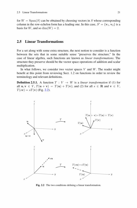
Definition 2.5.1. A function T : V → W is a linear transformation if (1) forall u,v ∈ V , T (u + v) = T (u) + T (v); and (2) for all s ∈ R and v ∈ V ,T (sv) = sT (v) (Fig. 2.2).
x
y
z
u
su
T
x
y
z
T (u)
T(su)=sT(u)
x
y
z
u
v
u+v
T
x
y
z
T(u)T(v)
T(u + v)=T(u) + T(v)
Fig. 2.2 The two conditions defining a linear transformation.
22 2 Linear Algebra Essentials
The two requirements for a function to be a linear transformation correspondexactly to the two vector space operations—the “structure”—on the sets V and W .The correct way of understanding these properties is to think of the function as“commuting” with the vector space operations: Performing the operation first (inV ) and then applying the function yields the same result as applying the functionfirst and then performing the operations (in W ). It is in this sense that lineartransformations “preserve the vector space structure.”
We recall some elementary properties of linear transformations that are conse-quences of Definition 2.5.1.
Theorem 2.5.2. Let V and W be vector spaces with corresponding zero vectors0V and 0W . Let T : V → W be a linear transformation. Then
1. T (0V ) = 0W .2. For all u ∈ V , T (−u) = −T (u).
Proof. Keeping in mind Theorem 2.1.2, both of these statements are consequencesof the second condition in Definition 2.5.1, using s = 0 and s = −1 respectively.
��The one-to-one, onto linear transformations play a special role in linear algebra.
They allow one to say that two different vector spaces are “the same.”
Definition 2.5.3. Suppose V and W are vector spaces. A linear transformation T :V → W is a linear isomorphism if it is one-to-one and onto. Two vector spaces Vand W are said to be isomorphic if there is a linear isomorphism T : V → W .
The most basic example of a linear isomorphism is the identity transformationIdV : V → V given by IdV (v) = v. We shall see other examples shortly.
The concept of linear isomorphism is an example of a recurring notion inthis text. The fact that an isomorphism between vector spaces V and W is one-to-one and onto says that V and W are the “same” as sets; there is a pairingbetween vectors in V and W . The fact that a linear isomorphism is in fact a lineartransformation further says that V and W have the same structure. Hence when Vand W are isomorphic as vector spaces, they have the “same” sets and the “same”structure, making them mathematically the same (different only possibly in thenames or characterizations of the vectors). This notion of isomorphism as samenesspervades mathematics. We shall see it again later in the context of geometricstructures.
One important feature of one-to-one functions is that they admit an inversefunction from the range of the original function to the domain of the originalfunction. In the case of a one-to-one, onto function T : V → W , the inverseT−1 : W → V is defined on all of W , where T ◦ T−1 = IdW and T−1 ◦ T = IdV .We summarize this in the following theorem.
Theorem 2.5.4. Let T : V → W be a linear isomorphism. Then there is a uniquelinear isomorphism T−1 : W → V such that T ◦ T−1 = IdW and T−1 ◦T = IdV .
2.6 Constructing Linear Transformations 23
Proof. Exercise. The most important fact to be proved is that the inverse of a lineartransformation, which exists purely on set-theoretic grounds, is in fact a lineartransformation. ��
We conclude with one sense in which isomorphic vector spaces have the samestructure. We will see others throughout the chapter.
Theorem 2.5.5. Suppose that V and W are finite-dimensional vector spaces, andsuppose there is a linear isomorphism T : V → W . Then dimV = dimW .
Proof. If {v1, . . . ,vn} is a basis for V , the reader can show that
{T (v1), . . . , T (vn)}
is a basis for W and that T (v1), . . . , T (vn) are distinct. ��
2.6 Constructing Linear Transformations
In this section we present two theorems that together generate a wealth of examplesof linear transformations. In fact, for pairs of finite-dimensional vector spaces, thesegive a method that generates all possible linear transformations between them.
The first theorem should be familiar to readers who have been exposed to afirst course in linear algebra. It establishes a basic correspondence between m × nmatrices and linear transformations between Euclidean spaces.
Theorem 2.6.1. Every linear transformation T : Rn → Rm can be expressed interms of matrix multiplication in the following sense: There exists an m× n matrixAT = [T ] such that T (x) = ATx, where x ∈ Rn is understood as a columnvector. Conversely, every m × n matrix A gives rise to a linear transformationTA : Rn → Rm by defining TA(x) = Ax.
For example, the linear transformation T : R3 → R2 given by
T (x, y, z) = (2x+ y − z, x+ 3z)
can be expressed as T (x) = ATx, where
AT =
[2 1 − 1
1 0 3
]
.
The proof of the first, main, statement of this theorem will emerge in the courseof this section. The second statement is a consequence of the basic properties ofmatrix multiplication.
The most important of several basic features of the correspondence betweenmatrices and linear transformations is that matrix multiplication corresponds tocomposition of linear transformations:
24 2 Linear Algebra Essentials
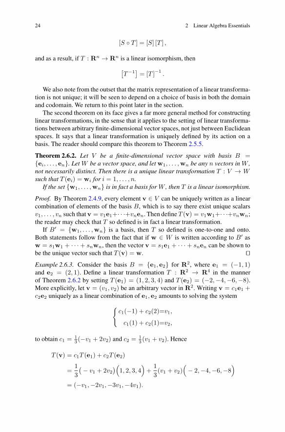
[S ◦ T ] = [S] [T ] ,
and as a result, if T : Rn → Rn is a linear isomorphism, then
[T−1
]= [T ]−1 .
We also note from the outset that the matrix representation of a linear transforma-tion is not unique; it will be seen to depend on a choice of basis in both the domainand codomain. We return to this point later in the section.
The second theorem on its face gives a far more general method for constructinglinear transformations, in the sense that it applies to the setting of linear transforma-tions between arbitrary finite-dimensional vector spaces, not just between Euclideanspaces. It says that a linear transformation is uniquely defined by its action on abasis. The reader should compare this theorem to Theorem 2.5.5.
Theorem 2.6.2. Let V be a finite-dimensional vector space with basis B ={ei, . . . , en}. Let W be a vector space, and let w1, . . . ,wn be any n vectors in W ,not necessarily distinct. Then there is a unique linear transformation T : V → Wsuch that T (ei) = wi for i = 1, . . . , n.
If the set {w1, . . . ,wn} is in fact a basis for W , then T is a linear isomorphism.
Proof. By Theorem 2.4.9, every element v ∈ V can be uniquely written as a linearcombination of elements of the basis B, which is to say there exist unique scalarsv1, . . . , vn such thatv = v1e1+· · ·+vnen. Then define T (v) = v1w1+· · ·+vnwn;the reader may check that T so defined is in fact a linear transformation.
If B′ = {w1, . . . ,wn} is a basis, then T so defined is one-to-one and onto.Both statements follow from the fact that if w ∈ W is written according to B′ asw = s1w1 + · · ·+ snwn, then the vector v = s1e1 + · · ·+ snen can be shown tobe the unique vector such that T (v) = w. ��Example 2.6.3. Consider the basis B = {e1, e2} for R2, where e1 = (−1, 1)and e2 = (2, 1). Define a linear transformation T : R2 → R4 in the mannerof Theorem 2.6.2 by setting T (e1) = (1, 2, 3, 4) and T (e2) = (−2,−4,−6,−8).More explicitly, let v = (v1, v2) be an arbitrary vector in R2. Writing v = c1e1 +c2e2 uniquely as a linear combination of e1, e2 amounts to solving the system
{c1(−1) + c2(2)=v1,
c1(1) + c2(1)=v2,
to obtain c1 = 13 (−v1 + 2v2) and c2 = 1
3 (v1 + v2). Hence
T (v) = c1T (e1) + c2T (e2)
=1
3
(− v1 + 2v2)(
1, 2, 3, 4)+
1
3(v1 + v2)
(− 2,−4,−6,−8
)
= (−v1,−2v1,−3v1,−4v1).
2.6 Constructing Linear Transformations 25
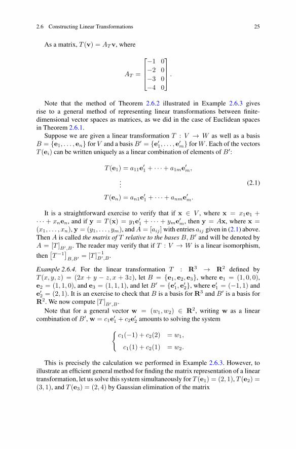
As a matrix, T (v) = ATv, where
AT =
⎡
⎢⎢⎣
−1 0
−2 0
−3 0
−4 0
⎤
⎥⎥⎦ .
Note that the method of Theorem 2.6.2 illustrated in Example 2.6.3 givesrise to a general method of representing linear transformations between finite-dimensional vector spaces as matrices, as we did in the case of Euclidean spacesin Theorem 2.6.1.
Suppose we are given a linear transformation T : V → W as well as a basisB = {e1, . . . , en} for V and a basis B′ = {e′1, . . . , e′m} for W . Each of the vectorsT (ei) can be written uniquely as a linear combination of elements of B′:
T (e1) = a11e′1 + · · ·+ a1me′m,
...
T (en) = an1e′1 + · · ·+ anme′m.
(2.1)
It is a straightforward exercise to verify that if x ∈ V , where x = x1e1 +· · · + xnen, and if y = T (x) = y1e
′1 + · · · + yme′m, then y = Ax, where x =
(x1, . . . , xn), y = (y1, . . . , ym), andA = [aij ] with entries aij given in (2.1) above.Then A is called the matrix of T relative to the bases B,B′ and will be denoted byA = [T ]B′,B . The reader may verify that if T : V → W is a linear isomorphism,
then[T−1
]
B,B′ = [T ]−1B′,B.
Example 2.6.4. For the linear transformation T : R3 → R2 defined byT (x, y, z) = (2x + y − z, x + 3z), let B = {e1, e2, e3}, where e1 = (1, 0, 0),e2 = (1, 1, 0), and e3 = (1, 1, 1), and let B′ = {e′1, e′2}, where e′1 = (−1, 1) ande′2 = (2, 1). It is an exercise to check that B is a basis for R3 and B′ is a basis forR2. We now compute [T ]B′,B .
Note that for a general vector w = (w1, w2) ∈ R2, writing w as a linearcombination of B′, w = c1e
′1 + c2e
′2 amounts to solving the system
{c1(−1) + c2(2) = w1,
c1(1) + c2(1) = w2.
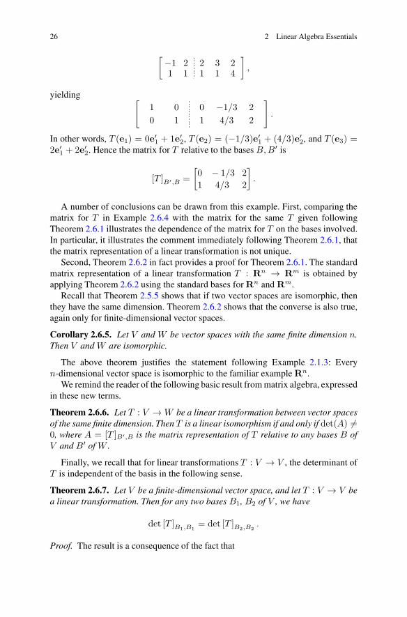
This is precisely the calculation we performed in Example 2.6.3. However, toillustrate an efficient general method for finding the matrix representation of a lineartransformation, let us solve this system simultaneously for T (e1) = (2, 1), T (e2) =(3, 1), and T (e3) = (2, 4) by Gaussian elimination of the matrix
26 2 Linear Algebra Essentials
[−1 2 2 3 21 1 1 1 4
]
,
yielding [1 0 0 −1/3 2
0 1 1 4/3 2
]
.
In other words, T (e1) = 0e′1 + 1e′2, T (e2) = (−1/3)e′1 + (4/3)e′2, and T (e3) =2e′1 + 2e′2. Hence the matrix for T relative to the bases B,B′ is
[T ]B′,B =
[0 − 1/3 2
1 4/3 2
]
.
A number of conclusions can be drawn from this example. First, comparing thematrix for T in Example 2.6.4 with the matrix for the same T given followingTheorem 2.6.1 illustrates the dependence of the matrix for T on the bases involved.In particular, it illustrates the comment immediately following Theorem 2.6.1, thatthe matrix representation of a linear transformation is not unique.
Second, Theorem 2.6.2 in fact provides a proof for Theorem 2.6.1. The standardmatrix representation of a linear transformation T : Rn → Rm is obtained byapplying Theorem 2.6.2 using the standard bases for Rn and Rm.
Recall that Theorem 2.5.5 shows that if two vector spaces are isomorphic, thenthey have the same dimension. Theorem 2.6.2 shows that the converse is also true,again only for finite-dimensional vector spaces.
Corollary 2.6.5. Let V and W be vector spaces with the same finite dimension n.Then V and W are isomorphic.
The above theorem justifies the statement following Example 2.1.3: Everyn-dimensional vector space is isomorphic to the familiar example Rn.
We remind the reader of the following basic result from matrix algebra, expressedin these new terms.
Theorem 2.6.6. Let T : V → W be a linear transformation between vector spacesof the same finite dimension. Then T is a linear isomorphism if and only if det(A) �=0, where A = [T ]B′,B is the matrix representation of T relative to any bases B ofV and B′ of W .
Finally, we recall that for linear transformations T : V → V , the determinant ofT is independent of the basis in the following sense.
Theorem 2.6.7. Let V be a finite-dimensional vector space, and let T : V → V bea linear transformation. Then for any two bases B1, B2 of V , we have
det [T ]B1,B1= det [T ]B2,B2
.
Proof. The result is a consequence of the fact that

2.7 Constructing Subspaces II: Subspaces and Linear Transformations 27
[T ]B2,B2= [Id]B2,B1
[T ]B1,B1[Id]B1,B2
,
and that [Id]B2,B1= [Id]−1
B1,B2, where Id : V → V is the identity transformation.
��For this reason, we refer to the determinant of the linear transformation T : V →
V and write det(T ) to be the value of det(A), where A = [T ]B,B for any basis Bof V .
2.7 Constructing Subspaces II: Subspaces and LinearTransformations
There are several subspaces naturally associated with a linear transformation T :V → W .
Definition 2.7.1. The kernel of a linear transformation of T : V → W , denoted byker(T ), is defined to be the set
ker(T ) = {v ∈ V | T (v) = 0} ⊂ V.
Definition 2.7.2. The range of a linear transformation T : V → W , denoted byR(T ), is defined to be the set
R(T ) = {w ∈ W | there is v ∈ V such that T (v) = w} ⊂ W.
Theorem 2.7.3. Let T : V → W be a linear transformation. Then ker(T ) andR(T ) are subspaces of V and W respectively.
Proof. Exercise. ��It is a standard exercise in a first course in linear algebra to find a basis for the
kernel of a given linear transformation.
Example 2.7.4. Let T : R3 → R be given by T (x, y, z) = ax + by + cz, wherea, b, c are not all zero. Then
ker(T ) = {(x, y, z) | ax+ by + cz = 0},
the subspace we encountered in Example 2.2.6. Suppose that a �= 0. Then we canalso write
ker(T ) = {(−bs− ct, as, at) | s, t ∈ R} .The set S = {b1,b2}, where b1 = (−b, a, 0) and b2 = (−c, 0, a), is a basis forker(T ), and so dim(ker(T )) = 2.
28 2 Linear Algebra Essentials
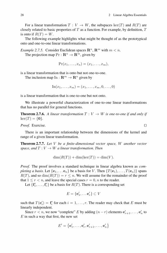
For a linear transformation T : V → W , the subspaces ker(T ) and R(T ) areclosely related to basic properties of T as a function. For example, by definition, Tis onto if R(T ) = W .
The following example highlights what might be thought of as the prototypicalonto and one-to-one linear transformations.
Example 2.7.5. Consider Euclidean spaces Rn, Rm with m < n.The projection map Pr : Rn → Rm, given by
Pr(x1, . . . , xn) = (x1, . . . , xm),
is a linear transformation that is onto but not one-to-one.The inclusion map In : Rm → Rn given by
In(x1, . . . , xm) = (x1, . . . , xm, 0, . . . , 0)
is a linear transformation that is one-to-one but not onto.
We illustrate a powerful characterization of one-to-one linear transformationsthat has no parallel for general functions.
Theorem 2.7.6. A linear transformation T : V → W is one-to-one if and only ifker(T ) = {0}.
Proof. Exercise. ��There is an important relationship between the dimensions of the kernel and
range of a given linear transformation.
Theorem 2.7.7. Let V be a finite-dimensional vector space, W another vectorspace, and T : V → W a linear transformation. Then
dim(R(T )) + dim(ker(T )) = dim(V ).
Proof. The proof involves a standard technique in linear algebra known as com-pleting a basis. Let {e1, . . . en} be a basis for V . Then {T (e1), . . . , T (en)} spansR(T ), and so dim(R(T )) = r ≤ n. We will assume for the remainder of the proofthat 1 ≤ r < n, and leave the special cases r = 0, n to the reader.
Let {f ′1, . . . , f ′r} be a basis for R(T ). There is a corresponding set
E = {e′1, . . .e′r} ⊂ V
such that T (e′i) = f ′i for each i = 1, . . . , r. The reader may check that E must belinearly independent.
Since r < n, we now “complete” E by adding (n− r) elements e′r+1, . . . , e′n to
E in such a way that first, the new set
E′ ={e′1, . . . , e
′r, e
′r+1, . . . , e
′n
}
2.7 Constructing Subspaces II: Subspaces and Linear Transformations 29
forms a basis for V , and second, that the set{e′r+1, . . . , e
′n
}forms a basis
for ker(T ). We illustrate the first step of this process. Choose br+1 /∈Span {e′1, . . . , e′r}. Since {f ′1, . . . , f ′r} is a basis for R(T ), write T (br+1) =
∑aif
′i
and define e′r+1 = br+1 − ∑aie
′i. Then the reader can verify that e′r+1 is still
independent of E and that T (e′r+1) = 0, so e′r+1 ∈ ker(T ). Form the new setE ∪ {
e′r+1
}. Repeated application of this process yields E′. We leave to the reader
the verification that{e′r+1, . . . , e
′n
}forms a basis for ker(T ). ��
We will frequently refer to the dimension of the range of a linear transformation.
Definition 2.7.8. The rank of a linear transformation T : V → W is the dimensionof R(T ).
The reader can verify that this definition of rank matches exactly that of the rankof any matrix representative of T relative to bases for V and W .
The following example illustrates both the statement of Theorem 2.7.7 and thenotion of completing a basis used in the theorem’s proof.
Example 2.7.9. Let V be a vector space with dimension n and let W be a subspaceof V with dimension r, with 1 ≤ r < n. Let B′ = {e1, . . .er} be a basis for W .Complete this basis to a basis B = {e1, . . . , er, er+1, . . . , en} for V .
We define a linear transformation PrB′,B : V → V as follows: For every vectorv ∈ V , there are unique scalars v1, . . . , vn such that v = v1e1+ · · ·+ vnen. Define
PrB′,B(v) = v1e1 + · · ·+ vrer.
We leave it as an exercise to show that PrB′,B is a linear transformation. ClearlyW = R(PrB′,B), and so dim(R(PrB′,B)) = r. Theorem 2.7.7 then implies thatdim(ker(PrB′,B)) = n− r, a fact that is also seen by noting that {er+1, . . . , en} isa basis for ker(PrB′,B).
As the notation implies, the map PrB′,B depends on the choices of bases B′ andB, not just on the subspace W .
Note that this example generalizes the projection defined in Example 2.7.5above.
Theorem 2.7.7 has a number of important corollaries for finite-dimensionalvector spaces. We leave the proofs to the reader.
Corollary 2.7.10. Let T : V → W be a linear transformation between finite-dimensional vector spaces. If T is one-to-one, then dim(V ) ≤ dim(W ). If T isonto, then dim(V ) ≥ dim(W ).
Note that this corollary gives another proof of Theorem 2.5.5.As an application of the above results, we make note of the following corollary,
which has no parallel in the nonlinear context.
Corollary 2.7.11. Let T : V → W be a linear transformation between vectorspaces of the same finite dimension. Then T is one-to-one if and only if T isonto.
30 2 Linear Algebra Essentials
2.8 The Dual of a Vector Space, Forms, and Pullbacks
This section, while fundamental to linear algebra, is not generally presented in afirst course on linear algebra. However, it is the algebraic foundation for the basicobjects of differential geometry, differential forms, and tensors. For that reason, wewill be more explicit with our proofs and explanations.
Starting with a vector space V , we will construct a new vector space V ∗. Further,given vector spaces V and W along with a linear transformation Ψ : V → W , wewill construct a new linear transformation Ψ∗ : W ∗ → V ∗ associated to Ψ .
Let V be a vector space. Define the set V ∗ to be the set of all linear transforma-tions from V to R:
V ∗ = {T : V → R | T is a linear transformation} .
Note that an element T ∈ V ∗ is a function. Define the operations of addition andscalar multiplication on V ∗ pointwise in the manner of Example 2.1.4. In otherwords, for T1, T2 ∈ V ∗, define T1 + T2 ∈ V ∗ by (T1 + T2)(v) = T1(v) + T2(v)for all v ∈ V , and for s ∈ R and T ∈ V ∗, define sT ∈ V ∗ by (sT )(v) = sT (v)for all v ∈ V .
Theorem 2.8.1. The set V ∗, equipped with the operations of pointwise additionand scalar multiplication, is a vector space.
Proof. The main item requiring proof is to demonstrate the closure axioms. SupposeT1, T2 ∈ V ∗. Then for every v1,v2 ∈ V , we have
(T1 + T2)(v1 + v2) = T1(v1 + v2) + T2(v1 + v2)
= (T1(v1) + T1(v2)) + (T2(v1) + T2(v2))
= (T1 + T2)(v1) + (T1 + T2)(v2).
We have relied on the linearity of T1 and T2 in the second equality. The proof that(T1 + T2)(cv) = c(T1 + T2)(v) for every c ∈ R and v ∈ V is identical. HenceT1 + T2 ∈ V ∗.
The fact that sT1 is also linear for every s ∈ R is proved similarly. Note that thezero “vector” O ∈ V ∗ is defined by O(v) = 0 for all v ∈ V . ��
The space V ∗ is called the dual vector space to V . Elements of V ∗ are variouslycalled dual vectors, linear one-forms, or covectors.
The proof of the following theorem, important in its own right, includes aconstruction that we will rely on often: the basis dual to a given basis.
Theorem 2.8.2. Suppose that V is a finite-dimensional vector space. Then
dim(V ) = dim(V ∗).

2.8 The Dual of a Vector Space, Forms, and Pullbacks 31
Proof. Let B = {e1, . . . , en} be a basis for V . We will construct a basis of V ∗
having n covectors.For i = 1, . . . , n, define covectors εi ∈ V ∗ by how they act on the basis B
according to Theorem 2.6.2: εi(ei) = 1 and εi(ej) = 0 for j �= i. In other words,for v = v1e1 + · · ·+ vnen,
εi(v) = vi.
We show that B∗ = {ε1, . . . , εn} is a basis for V ∗. To show that B∗ islinearly independent, suppose that c1ε1 + · · · + cnεn = O (an equality of lineartransformations). This means that for all v ∈ V ,
c1ε1(v) + · · ·+ cnεn(v) = O(v) = 0.
In particular, for each i = 1, . . . , n, setting v = ei gives
0 = c1ε1(ei) + · · ·+ cnεn(ei)
= ci.
Hence B∗ is a linearly independent set.To show that B∗ spans V ∗, choose an arbitrary T ∈ V ∗, i.e., T : V → R is a
linear transformation. We need to find scalars c1, . . . , cn such that T = c1ε1+ · · ·+cnεn. Following the idea of the preceding argument for linear independence, defineci = T (ei).
We need to show that for all v ∈ V ,
T (v) = (c1ε1 + · · ·+ cnεn)(v).
Let v = v1e1 + · · ·+ vnen. On the one hand,
T (v) = T (v1e1 + · · ·+ vnei)
= v1T (e1) + · · ·+ vnT (en)
= v1c1 + · · ·+ vncn.
On the other hand,
(c1ε1 + · · ·+ cnεn)(v) = c1ε1(v) + · · ·+ cnεn(v)
= c1v1 + · · ·+ cnvn.
Hence T = c1ε1 + · · ·+ cnεn, and B∗ spans V ∗. ��Definition 2.8.3. Let B = {e1, . . . , en} be a basis for V . The basis B∗ ={ε1, . . . , εn} for V ∗, where εi : V → R are linear transformations defined bytheir action on the basis vectors as

32 2 Linear Algebra Essentials
εi(ej) =
{1 if i = j,
0 if i �= j,
is called the basis of V ∗ dual to the basis B.
Example 2.8.4. Let B0 = {e1, . . . , en} be the standard basis for Rn, i.e.,
ei = (0, . . . , 0, 1, 0, . . . , 0),
with 1 in the ith component (see Example 2.4.6). The basis B∗0 = {ε1, . . . , εn} dual
to B0 is known as the standard basis for (Rn)∗. Note that if v = (v1, . . . , vn), thenεi(v) = vi. In other words, in the language of Example 2.7.5, εi is the projectiononto the ith component.
We note that Theorem 2.6.1 gives a standard method of writing a lineartransformation T : Rn → Rm as an m× n matrix. Linear one-forms T ∈ (Rn)∗,T : Rn → R, are no exception. In this way, elements of (Rn)∗ can be thought ofas 1 × n matrices, i.e., as row vectors. For example, the standard basis B∗
0 in thisnotation would appear as
[ε1] =[1 0 · · · 0] ,
...
[εn] =[0 0 · · · 1] .
We now apply the “dual” construction to linear transformations between vectorspaces V and W . For a linear transformation Ψ : V → W , we will construct a newlinear transformation
Ψ∗ : W ∗ → V ∗.
(Note that this construction “reverses the arrow” of the transformation Ψ .)Take an element of the domain T ∈ W ∗, i.e., T : W → R is a linear
transformation. We wish to assign to T a linear transformation S = Ψ∗(T ) ∈ V ∗.In other words, given T ∈ W ∗, we want to be able to describe a map S : V → R,S(v) = (Ψ∗(T ))(v) for v ∈ V , in such a way that S has the properties of a lineartransformation.
Theorem 2.8.5. Let Ψ : V → W be a linear transformation and let Ψ∗ : W ∗ →V ∗ be given by
(Ψ∗(T ))(v) = T (Ψ(v))
for all T ∈ W ∗ and v ∈ V . Then Ψ∗ is a linear transformation.
The transformation Ψ∗ : W ∗ → V ∗ so defined is called the pullback mapinduced by Ψ , and Ψ∗(T ) is called the pullback of T by Ψ .
Proof. The first point to be verified is that for a fixed T ∈ W ∗, we have in factΨ∗(T ) ∈ V ∗. In other words, we need to show that if T : W → R is a linear

2.8 The Dual of a Vector Space, Forms, and Pullbacks 33
transformation, then Ψ∗(T ) : V → R is a linear transformation. For v1,v2 ∈ V ,we have
(Ψ∗(T ))(v1 + v2) = T (Ψ(v1 + v2))
= T (Ψ(v1) + Ψ(v2)) since Ψ is linear
= T (Ψ(v1)) + T (Ψ(v2)) since T is linear
= (Ψ∗(T ))(v1) + (Ψ∗(T ))(v2).
The proof that (Ψ∗(T ))(sv) = s(Ψ∗(T ))(v) for a fixed T and for any vectorv ∈ V and scalar s ∈ R is similar.
To prove linearity of Ψ∗ itself, suppose that s ∈ R and T ∈ W ∗. Then for allv ∈ V ,
(Ψ∗(sT ))(v) = (sT )(Ψ(v))
= sT (Ψ(v))
= s((Ψ∗(T ))(v)),
and so Ψ∗(sT ) = sΨ∗(T ).We leave as an exercise the verification that for all T1, T2 ∈ W ∗, Ψ∗(T1+T2) =
Ψ∗(T1) + Ψ∗(T2). ��Note that Ψ∗(T ) = T ◦ Ψ . It is worth mentioning that the definition of the
pullback in Theorem 2.8.5 is the sort of “canonical” construction typical of abstractalgebra. It can be expressed by the diagram
V W
R
TΨ ∗T
Ψ
Example 2.8.6 (The matrix form of a pullback). Let Ψ : R3 → R2 be given byΨ(x, y, z) = (2x+y−z, x+3z) and let T ∈ (R2)∗ be given by T (u, v) = u−5v.Then Ψ∗(T ) ∈ (R3)∗ is given by
(Ψ∗T )(x, y, z) = T (Ψ(x, y, z))
= T (2x+ y − z, x+ 3z)
= (2x+ y − z)− 5(x+ 3z)
= −3x+ y − 16z.

34 2 Linear Algebra Essentials
In the standard matrix representation of Theorem 2.6.1, we have
[Ψ ] =
[2 1 − 1
1 0 3
]
, [T ] =[1 − 5
]and [Ψ∗T ] =
[−3 1 − 16]= [T ] [Ψ ].
Thus the pullback operation by Ψ on linear one-forms corresponds to matrixmultiplication of a given row vector on the right by the matrix of Ψ .
This fact may seem strange to the reader who has become accustomed to lineartransformations represented as matrices acting by multiplication on the left. Itreflects the fact that all the calculations in the preceding paragraph were carriedout by relying on the standard bases in Rn and Rm as opposed to the dual bases for(Rn)∗ and (Rm)∗.
Let us reconsider these calculations, this time using the dual basis from Exam-ple 2.8.4 and the more general matrix representation from the method followingTheorem 2.6.2. Using the standard bases B0 = {ε1, ε2} for (R2)∗ and B′
0 ={ε′1, ε′2, ε′3} for (R3)∗, where ε1 =
[1 0
], ε2 =
[0 1
], ε′1 =
[1 0 0
],
ε′2 =[0 1 0
], and ε′3 =
[0 0 1
], we note that Ψ∗(ε1) = 2ε′1 + ε′2 − ε′3 and
Ψ∗(ε2) = ε′1 + 3ε′3. Hence
[Ψ∗]B′0,B0
=
⎡
⎣2 1
1 0
−1 3
⎤
⎦ = [Ψ ]T.
Now, when the calculations for the pullback of T = ε1 − 5ε2 by Ψ are written
using the column vector [T ]B0=
[1
−5
]
, we see that
[Ψ∗(T )]B′0= [Ψ∗]B′
0,B0[T ]B0
=
⎡
⎣2 1
1 0
−1 3
⎤
⎦
[1
−5
]
=
⎡
⎣−3
1
−16
⎤
⎦ .
Since the pullback of a linear transformation is related to the matrix transpose,as the example illustrates, the following property is not surprising in light of thefamiliar property (AB)T = BTAT .
Proposition 2.8.7. Let Ψ1 : V1 → V2 and Ψ2 : V2 → V3 be linear transformations.Then
(Ψ2 ◦ Ψ1)∗ = Ψ∗
1 ◦ Ψ∗2 .
Proof. Let T ∈ V ∗3 and choose v ∈ V1. Then on the one hand,
2.8 The Dual of a Vector Space, Forms, and Pullbacks 35
(Ψ2 ◦ Ψ1)∗(T )(v) = T ((Ψ2 ◦ Ψ1)(v))
= T (Ψ2(Ψ1(v))),
while on the other hand,
(Ψ∗1 ◦ Ψ∗
2 )(T )(v) = (Ψ∗1 (Ψ
∗2 (T )))(v)
= (Ψ∗1 (T ◦ Ψ2))(v)
= ((T ◦ Ψ2) ◦ Ψ1)(v)
= T (Ψ2(Ψ1(v))). ��
The construction of the dual space V ∗ is a special case of a more generalconstruction. Suppose we are given several vector spaces V1, . . . , Vk. Recall (seeSect. 1.1) that the Cartesian product of V1, . . . , Vk is the set of ordered k-tuples ofvectors
V1 × · · · × Vk = {(v1, . . . ,vk) | vi ∈ Vi for all i = 1, . . . , k} .
The set V = V1 × · · · × Vk can be given the structure of a vector space by definingvector addition and scalar multiplication componentwise.
Definition 2.8.8. Let V1, . . . , Vk and W be vector spaces. A function
T : V1 × · · · × Vk → W
is multilinear if it is linear in each component:
T (x1 + y,x2, . . . ,xk) = T (x1,x2, . . . ,xk) + T (y,x2, . . . ,xk),
...
T (x1,x2, . . . ,xk−1,xk+y)=T (x1,x2, . . . ,xk−1,xk)+T (x1,x2, . . . ,xk−1,y),
andT (sx1,x2, . . . ,xk) = sT (x1,x2, . . . ,xk),
...
T (x1,x2, . . . , sxk) = sT (x1,x2, . . . ,xk).
In the special case that all the Vi are the same and W = R, then a multilinearfunction T : V × · · · × V → R is called a multilinear k-form on V .
Example 2.8.9 (The zero k-form on V ). The trivial example of a k-form on a vectorspace V is the zero form. Define O(v1, . . . ,vk) = 0 for all v1, . . . ,vk ∈ V . Weleave it to the reader to show that O is multilinear.

36 2 Linear Algebra Essentials
Example 2.8.10 (The determinant as an n-form on Rn). Define the map Ω : Rn ×· · · ×Rn → R by
Ω(a1, . . . , an) = detA,
where A is the matrix whose columns are given by the vectors ai ∈ Rn relativeto the standard basis: A = [a1 · · · an] . The fact that Ω is an n-form follows fromproperties of the determinant of matrices.
In the work that follows, we will see several important examples of bilinearforms (i.e., 2-forms) on Rn.
Example 2.8.11. Let G0 : Rn ×Rn → R be the function defined by
G0(x,y) = x1y1 + · · ·+ xnyn,
where x = (x1, . . . , xn) and y = (y1, . . . , yn). ThenG0 is a bilinear form. (Readersshould recognize G0 as the familiar “dot product” of vectors in Rn.) We leave it asan exercise to verify the linearity of G0 in each component. Note that G0(x,y) =G0(y,x) for all x,y ∈ Rn.
Example 2.8.12. Let A be an n × n matrix and let G0 be the bilinear form on Rn
defined in the previous example. Then define GA : Rn ×Rn → R by GA(x,y) =G0(Ax, Ay). Bilinearity of GA is a consequence of the bilinearity of G0 and thelinearity of matrix multiplication:
GA(x1 + x2,y) = G0(A(x1 + x2), Ay)
= G0(Ax1 +Ax2, Ay)
= G0(Ax1, Ay) +G0(Ax2, Ay)
= GA(x1,y) +GA(x2,y),
andGA(sx,y) = G0(A(sx), Ay)
= G0(sAx, Ay)
= sG0(Ax, Ay)
= sGA(x,y).
Linearity in the second component can be shown in the same way, or the readermay note that GA(x,y) = GA(y,x) for all x,y ∈ Rn.
Example 2.8.13. Define S : R2 × R2 → R by S(x,y) = x1y2 − x2y1, wherex = (x1, x2) and y = (y1, y2). For z = (z1, z2), we have
S(x+ z,y) = (x1 + z1)y2 − (x2 + z2)y1
= (x1y2 − x2y1) + (z1y2 − z2y1)
= S(x,y) + S(z,y).
2.9 Geometric Structures I: Inner Products 37
Similarly, for every c ∈ R, S(cx,y) = cS(x,y). Hence S is linear in the firstcomponent. Linearity in the second component then follows from the fact thatS(y,x) = −S(x,y) for all x,y ∈ R2. This shows that S is a bilinear form.
Let V be a vector space of dimensionn, and let b : V×V → R be a bilinear form.There is a standard way to represent b by means of an n × n matrix B, assumingthat a basis is specified.
Proposition 2.8.14. Let V be a vector space with basis E = {e1, . . . , en} and letb : V × V → R be a bilinear form. Let B = [bij ], where bij = b(ei, ej). Then forevery v,w ∈ V , we have
b(v,w) = wTBv,
where v and w are written as column vectors relative to the basis E .
Proof. On each side, write v and w as linear combinations of the basis vectorse1, . . . , en. The result follows from the bilinearity of b and the linearity of matrixmultiplication. ��
This proposition allows us to study properties of the bilinear form b by means ofproperties of its matrix representation B, a fact that we will use in the future. Notethat the matrix representation for GA in Example 2.8.12 relative to the standardbasis for Rn is ATA.
Finally, the pullback operation can be extended to multilinear forms. We illustratethis in the case of bilinear forms, although we will return to this topic in moregenerality in Chap. 4.
Definition 2.8.15. Suppose T : V → W is a linear transformation between vectorspaces V and W . Let B : W ×W → R be a bilinear form on W . Then the pullbackof B by T is the bilinear form T ∗B : V × V → R defined by
(T ∗B)(v1,v2) = B(T (v1), T (v2))
for all v1,v2 ∈ V .
The reader may check that T ∗B so defined is in fact a bilinear form.
Proposition 2.8.16. Let U , V , and W be vector spaces and let T1 : U → V andT2 : V → W be linear transformations. Let B : W ×W → R be a bilinear formon W . Then
(T2 ◦ T1)∗B = T ∗
1 (T∗2B).
Proof. The proof is a minor adaptation of the proof of Proposition 2.8.7. ��
2.9 Geometric Structures I: Inner Products
There are relatively few traditional geometric concepts that can be defined strictlywithin the axiomatic structure of vector spaces and linear transformations aspresented above. One that we might define, for example, is the notion of two vectors
38 2 Linear Algebra Essentials
being parallel: For two vectors v,w in a vector space V , we could say that v isparallel to w if there is a scalar s ∈ R such that w = sv.
The notion of vectors being perpendicular might also be defined in a crude wayby means of the projection map of Example 2.7.9. Namely, a vector v ∈ V couldbe defined to be perpendicular to a nonzero vector w ∈ V if v ∈ kerPrB′,B, whereB′ = {w} and B is chosen to be a basis for V whose first vector is w. This hasthe distinct disadvantage of being completely dependent on the choice of basis B,in the sense that a vector might be perpendicular to another vector with respect toone basis but not with respect to another.
The reader should note that both these attempts at definitions of basic geometricnotions are somewhat stilted, since we are defining the terms parallel and perpen-dicular without reference to the notion of angle. In fact, we have already noted thatin the entire presentation of linear algebra up to this point, two notions traditionallyassociated with vectors—magnitude and direction—have not been defined at all.These notions do not have a natural description using the vector space axioms alone.
The notions of magnitude and direction can be described easily, however, bymeans of an additional mathematical structure that generalizes the familiar “dotproduct” (Example 2.8.11).
Definition 2.9.1. An inner product on a vector space V is a functionG : V × V → R with the following properties:
(I1) G is a bilinear form;(I2) G is symmetric: For all v,w ∈ V , G(v,w) = G(w,v);(I3) G is positive definite: For all v ∈ V , G(v,v) ≥ 0, with G(v,v) = 0 if and
only if v = 0.
The pair (V,G) is called an inner product space.
We mention that the conditions (I1)–(I3) imply that the matrix A correspondingto the bilinear formG according to Proposition 2.8.14 must be symmetric (AT = A)and positive definite (xTAx ≥ 0 for all x ∈ Rn, with equality only when x = 0).
Example 2.9.2 (The dot product). On the vector space Rn, define G0(v,w) =v1w1 + · · · + vnwn, where v = (v1, . . . , vn) and w = (w1, . . . , wn). We sawin Example 2.8.11 that G0 is a bilinear form on Rn. The reader may verify property(I2). To see property (I3), note that G0(v,v) = v21 + · · · + v2n is a quantity that isalways nonnegative and is zero exactly when v1 = · · · = vn = 0, i.e., when v = 0.
Note that Example 2.9.2 can be generalized to any finite-dimensional vectorspace V . Starting with any basis B = {e1, . . . , en} for V , define GB(v,w) =v1w1 + · · ·+ vnwn, where v = v1e1 + · · ·+ vnen and w = w1e1 + · · ·+ wnen.This function GB is well defined because of the unique representation of v and win the basis B. This observation proves the following:
Theorem 2.9.3. Every finite-dimensional vector space carries an inner productstructure.
2.9 Geometric Structures I: Inner Products 39
Of course, there is no unique inner product structure on a given vector space.The geometry of an inner product space will be determined by the choice of innerproduct.
It is easy to construct new inner products from a given inner product structure.We illustrate one method in Rn, starting from the standard inner product inExample 2.9.2 above.
Example 2.9.4. Let A be any invertible n × n matrix. Define a bilinear form GA
on Rn as in Example 2.8.12: GA(v,w) = G0(Av, Aw), where G0 is the standardinner product from Example 2.9.2. Then GA is symmetric, since G0 is symmetric.Similarly, GA(v,v) ≥ 0 for all v ∈ V because of the corresponding property ofG0. Now suppose that GA(v,v) = 0. Since 0 = GA(v,v) = G0(Av, Av), wehave Av = 0 by property (I3) for G0. Since A is invertible, v = 0. This completesthe verification that GA is an inner product on Rn.
To illustrate this construction with a simple example in R2, consider the matrix
A =
[2 −1
1 0
]
. Then if v = (v1, v2) and w = (w1, w2), we have
GA(v,w) = G0(Av, Aw)
= G0
((2v1 − v2, v1), (2w1 − w2, w1)
)
= (2v1 − v2)(2w1 − w2) + v1w1
= 5v1w1 − 2v1w2 − 2v2w1 + v2w2.
Note that the matrix representation for GA as described in Proposition 2.8.14 isgiven by ATA.
An inner product allows us to define geometric notions such as length, distance,magnitude, angle, and direction.
Definition 2.9.5. Let (V,G) be an inner product space. The magnitude (also calledthe length or the norm) of a vector v ∈ V is given by
||v|| = G(v,v)1/2 .
The distance between vectors v and w is given by
d(v,w) = ||v −w|| = G(v −w,v −w)1/2.
To define the notion of direction, or angle between vectors, we first state afundamental property of inner products.
Theorem 2.9.6 (Cauchy–Schwarz). Let (V,G) be an inner product space. Thenfor all v,w ∈ V ,
|G(v,w)| ≤ ||v|| · ||w||.
40 2 Linear Algebra Essentials
The standard proof of the Cauchy–Schwarz inequality relies on the non-intuitiveobservation that the discriminant of the quadratic expression (in t) G(tv +w, tv+w) must be nonpositive by property (I3).
Definition 2.9.7. Let (V,G) be an inner product space. For every two nonzerovectors v,w ∈ V , the angle ∠G(v,w) between v and w is defined to be
∠G(v,w) = cos−1
(G(v,w)
||v|| · ||w||)
.
Note that this definition of angle is well defined as a result of Theorem 2.9.6.As a consequence of this definition of angle, it is possible to define a notion of
orthogonality: Two vectors v,w ∈ V are orthogonal if G(v,w) = 0, since then∠G(v,w) = π/2. The notion of orthogonality, in turn, distinguishes “special” basesfor V and provides a further method for producing new subspaces of V from a givenset of vectors in V .
Theorem 2.9.8. Let (V,G) be an inner product space with dim(V ) = n > 0.There exists a basis B = {u1, . . . ,un} satisfying the following two properties:
(O1) For each i = 1, . . . , n, G(ui,ui) = 1;(O2) For each i �= j, G(ui,uj) = 0.
Such a basis is known as an orthonormal basis.
The reader is encouraged to review the proof of this theorem, which can be foundin any elementary linear algebra text. It relies on an important procedure, similar inspirit to the proof of Theorem 2.7.7, known as Gram–Schmidt orthonormalization.Beginning with any given basis, the procedure gives a way of constructing a newbasis satisfying (O1) and (O2). In the next section, we will carry out the details ofan analogous procedure in the symplectic setting.
As with bases in general, there is no unique orthonormal basis for a given innerproduct space (V,G).
We state without proof a kind of converse to Theorem 2.9.8. This theorem isactually a restatement of the comment following Example 2.9.2.
Theorem 2.9.9. Let V be a vector space and let B = {e1, . . . , en} be a finite basisfor V . Define a function GB by requiring that
GB(ei, ej) =
{1 if i = j,
0 if i �= j,
and extending linearly in both components in the manner of Theorem 2.6.2. ThenGB is an inner product.
For any vector v in an inner product space (V,G), the set W of all vectorsorthogonal to v can be seen to be a subspace of V . One could appeal directly toTheorem 2.2.2 (since 0 ∈ W ), or one could note that W is the kernel of the linear

2.9 Geometric Structures I: Inner Products 41
transformation iv : V → R given by iv(w) = G(v,w). More generally, we havethe following:
Theorem 2.9.10. Let S be any nonempty set of vectors in an inner product space(V,G). The set S⊥ defined by
S⊥ = {w ∈ V | For all v ∈ S, G(v,w) = 0}
is a subspace of V .
Proof. Exercise. ��The set S⊥ is called the orthogonal complement to S.
Example 2.9.11. Let S = {v} ⊂ R3, where v = (a, b, c) �= 0. Let G0 be thestandard inner product on R3 (see Example 2.9.2). Then
S⊥ = {(x, y, z) | ax+ by + cz = 0} .
See Example 2.2.4.
Example 2.9.12. Let A =
[2 −1
1 0
]
and let GA be the inner product defined on R2
according to Example 2.9.4. Let v = (1, 0), and let S = {v}. Then the reader mayverify that
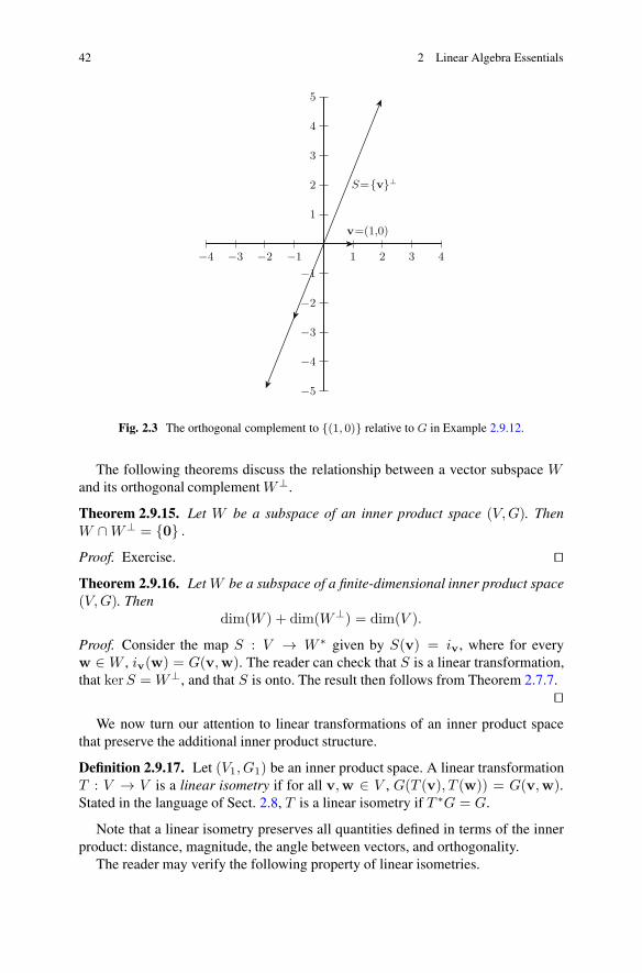
S⊥ = {(w1, w2) | 5w1 − 2w2 = 0} ,which is spanned by the set {(2, 5)}. See Fig. 2.3.
Theorem 2.9.13. Let (V,G) be an inner product space. Let S be a finite subset ofV and let W = Span(S). Then W⊥ = S⊥.
Proof. Let S = {w1, . . . ,wk}. Take a vector v ∈ W⊥, so that G(w,v) = 0 for allw ∈ W . In particular, since S ⊂ W , for each wi ∈ S, G(wi,v) = 0. So v ∈ S⊥
and W⊥ ⊂ S⊥.Now take a vector v ∈ S⊥. Let w ∈ W , so that there are scalars c1, . . . , ck such
that w = c1w1 + · · ·+ ckwk. Relying on the linearity of G in the first component,we obtain
G(w,v) = G(c1w1 + · · ·+ ckwk,v)
= G(c1w1,v) + · · ·+G(ckwk,v)
= c1G(w1,v) + · · ·+ ckG(wk,v)
= 0, since v ∈ S⊥.
Hence v ∈ W⊥, and so S⊥ ⊂ W⊥.Together, these two statements show that W⊥ = S⊥. ��
Corollary 2.9.14. Let B be a basis for a subspace W ⊂ V . Then W⊥ = B⊥.
42 2 Linear Algebra Essentials
1
2
3
4
5
−1
−2
−3
−4
−5
1 2 3 4−1−2−3−4
v=(1,0)
S={v}⊥
Fig. 2.3 The orthogonal complement to {(1, 0)} relative to G in Example 2.9.12.
The following theorems discuss the relationship between a vector subspace Wand its orthogonal complement W⊥.
Theorem 2.9.15. Let W be a subspace of an inner product space (V,G). ThenW ∩W⊥ = {0} .Proof. Exercise. ��Theorem 2.9.16. Let W be a subspace of a finite-dimensional inner product space(V,G). Then
dim(W ) + dim(W⊥) = dim(V ).
Proof. Consider the map S : V → W ∗ given by S(v) = iv, where for everyw ∈ W , iv(w) = G(v,w). The reader can check that S is a linear transformation,that kerS = W⊥, and that S is onto. The result then follows from Theorem 2.7.7.
��We now turn our attention to linear transformations of an inner product space
that preserve the additional inner product structure.
Definition 2.9.17. Let (V1, G1) be an inner product space. A linear transformationT : V → V is a linear isometry if for all v,w ∈ V , G(T (v), T (w)) = G(v,w).Stated in the language of Sect. 2.8, T is a linear isometry if T ∗G = G.
Note that a linear isometry preserves all quantities defined in terms of the innerproduct: distance, magnitude, the angle between vectors, and orthogonality.
The reader may verify the following property of linear isometries.
2.9 Geometric Structures I: Inner Products 43
Proposition 2.9.18. Let (V,G) be an inner product space. If T1, T2 are linearisometries of V , then T2 ◦ T1 is also a linear isometry.
The following theorem, which we state without proof, gives a matrix characteri-zation of linear isometries.
Theorem 2.9.19. Let (V,G) be a finite-dimensional inner product space withdim(V ) = n > 0, and let T : V → V be a linear isometry. Then the matrixrepresentation A = [T ] of T relative to any orthonormal basis of V satisfiesATA = In, where In is the n× n identity matrix.
A matrix with the property that ATA = In is called an orthogonal matrix.
Corollary 2.9.20. Let T : V → V be a linear isometry of a finite-dimensionalinner product space (V,G). Then det(T ) = ±1. In particular, T is invertible.
Proposition 2.9.21. Let (V,G) be a finite-dimensional inner product space, and letT : V → V be a linear isometry. Then its inverse T−1 is also a linear isometry.
Proof. Assuming T is a linear isometry, apply Proposition 2.8.16 to G = (Id)∗G =(T ◦ T−1)∗G and use the assumption that T ∗G = G. ��
We conclude this section with an important technical theorem, a consequence ofthe positive definite property of inner products. Recall that V and V ∗ have the samedimension by Theorem 2.8.2, and so by Corollary 2.6.5, the two vector spaces areisomorphic. A choice of an inner product on V , however, induces a distinguishedisomorphism between them.
Theorem 2.9.22. Let G be an inner product on a finite-dimensional vector spaceV . For every v ∈ V , define iv ∈ V ∗ by iv(w) = G(v,w) for w ∈ V . Then thefunction
Φ : V → V ∗
defined by Φ(v) = iv is a linear isomorphism.
Proof. The fact that Φ is linear is a consequence of the fact that G is bilinear. Forexample, for v ∈ V and s ∈ R, Φ(sv) = isv, and so for all w ∈ V , isv(w) =G(sv,w) = sG(v,w) = siv(w). Hence isv = siv, and so Φ(sv) = sΦ(v).Likewise, Φ(v +w) = Φ(v) + Φ(w) for all v,w ∈ V .
To show that Φ is one-to-one, we show that ker(Φ) = {0}. Let v ∈ ker(Φ). ThenΦ(v) = O, i.e., G(v,w) = 0 for all w ∈ V . In particular, G(v,v) = 0, and sov = 0 by positive definiteness. Hence ker(Φ) = {0}, and so by Theorem 2.7.6, Φis one-to-one.
The fact that Φ is onto now follows from the fact that a one-to-one linear mapbetween vector spaces of the same dimension must be onto (Corollary 2.7.11).However, we will show directly that Φ is onto in order to exhibit the inversetransformation Φ−1 : V ∗ → V .
Let T ∈ V ∗. We need to find vT ∈ V such that Φ(vT ) = T . Let {u1, . . . ,un}be an orthonormal basis for (V,G), as guaranteed by Theorem 2.9.8. Define ci by

44 2 Linear Algebra Essentials
ci = T (ui), and define vT = c1u1 + · · ·+ cnun. By the linearity of G in the firstcomponent, we have Φ(vT ) = T , or, what is the same, vT = Φ−1(T ). Hence Φ isonto. ��
The reader should notice the similarity between the construction of Φ−1 and theprocedure outlined in the proof of Theorem 2.8.2.
The fact that the map Φ in Theorem 2.9.22 is one-to-one can be rephrased bysaying that the inner product G is nondegenerate: If G(v,w) = 0 for all w ∈ V ,then v = 0. We will encounter this condition again shortly in the symplectic setting.
2.10 Geometric Structures II: Linear Symplectic Forms
In this section, we outline the essentials of linear symplectic geometry, which willbe the starting point for one of the main differential-geometric structures that wewill present later in the text. The presentation here will parallel the developmentof inner product structures in Sect. 2.9 in order to emphasize the similarities anddifferences between the two structures, both of which are defined by bilinear forms.We will discuss more about the background of symplectic geometry in Chap. 7.
Unlike most of the material in this chapter so far, what follows is not generallypresented in a first course in linear algebra. As in Sect. 2.8, we will be more detailedin the presentation and proof of the statements in this section.
Definition 2.10.1. A linear symplectic form on a vector space V is a function ω :V × V → R satisfying the following properties:
(S1) ω is a bilinear form on V ;(S2) ω is skew-symmetric: For all v,w ∈ V , ω(w,v) = −ω(v,w);(S3) ω is nondegenerate: If v ∈ V has the property that ω(v,w) = 0 for all w ∈ V ,
then v = 0.
The pair (V, ω) is called a symplectic vector space.
Note that the main difference between (S1)–(S3) and (I1)–(I3) in Definition 2.9.1is that a linear symplectic form is skew-symmetric, in contrast to the symmetricinner product. We can summarize properties (S1) and (S2) by saying that ω is analternating bilinear form on V . We will discuss the nondegeneracy condition (S3)in more detail below. Note that in sharp contrast to inner products, ω(v,v) = 0 forall v ∈ V as a consequence of (S2).
Example 2.10.2. On the vector space R2, define ω0(v,w) = v1w2 − v2w1,where v = (v1, v2) and w = (w1, w2). The reader may recognize this as thedeterminant of the matrix whose column vectors are v,w. That observation, ordirect verification, will confirm properties (S1) and (S2). To verify (S3), supposev = (v1, v2) is such that ω0(v,w) = 0 for all w ∈ R2. In particular,0 = ω0(v, (1, 0)) = (v1)(0) − (1)(v2) = −v2, and so v2 = 0. Likewise,
2.10 Geometric Structures II: Linear Symplectic Forms 45
1
2
1 2
w
v
|ω0(v,w)|=Area of R
R
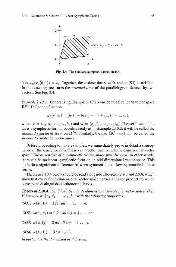
Fig. 2.4 The standard symplectic form on R2.
0 = ω0(v, (0, 1)) = v1. Together, these show that v = 0, and so (S3) is satisfied.In this case, ω0 measures the oriented area of the parallelogram defined by twovectors. See Fig. 2.4.
Example 2.10.3. Generalizing Example 2.10.2, consider the Euclidean vector spaceR2n. Define the function
ω0(v,w) = (a1t1 − b1s1) + · · ·+ (antn − bnsn),
where v = (a1, b1, . . . , an, bn) and w = (s1, t1, . . . , sn, tn). The verification thatω0 is a symplectic form proceeds exactly as in Example 2.10.2; it will be called thestandard symplectic form on R2n. Similarly, the pair (R2n, ω0) will be called thestandard symplectic vector space.
Before proceeding to more examples, we immediately prove in detail a conseq-uence of the existence of a linear symplectic form on a finite-dimensional vectorspace: The dimension of a symplectic vector space must be even. In other words,there can be no linear symplectic form on an odd-dimensional vector space. Thisis the first significant difference between symmetric and skew-symmetric bilinearforms.
Theorem 2.10.4 below should be read alongside Theorems 2.9.3 and 2.9.8, whichshow that every finite-dimensional vector space carries an inner product, to whichcorrespond distinguished orthonormal bases.
Theorem 2.10.4. Let (V, ω) be a finite-dimensional symplectic vector space. ThenV has a basis {e1, f1, . . . , en, fn} with the following properties:
(SO1) ω(ei, fi) = 1 for all i = 1, . . . , n;
(SO2) ω(ei, ej) = 0 for all i, j = 1, . . . , n;
(SO3) ω(fi, fj) = 0 for all i, j = 1, . . . , n;
(SO4) ω(ei, fj) = 0 for i �= j.
In particular, the dimension of V is even.

46 2 Linear Algebra Essentials
Proof. The inductive process of constructing a basis with properties (SO1)–(SO4)is a modified version of the Gram–Schmidt orthonormalization process that is at theheart of the proof of Theorem 2.9.8. The reader should also compare the techniquehere with the technique in the proof of Theorem 2.7.7.
Choose any nonzero v ∈ V and define e1 = v. Since e1 �= 0, property(S3) of the symplectic form guarantees the existence of a vector w1 such thatω(e1,w1) = c1 �= 0. Define f1 = (1/c1)w1. By the bilinearity condition (S1),we have ω(e1, f1) = 1. Note also that {e1, f1} is a linearly independent set, sinceotherwise, by Theorem 2.4.3 we would have a scalar s such that f1 = se1, and soby (S2), ω(e1, f1) = 0, contradicting the definition of f1. Further, by (S2), we haveω(e1, e1) = ω(f1, f1) = 0, and so the set {e1, f1} satisfies properties (SO1)–(SO4).
Now suppose we have constructed k pairs of linearly independent vectors
Bk = {e1, f1, . . . , ek, fk}
satisfying (SO1)–(SO4). If Span(Bk) = V , then Bk is the desired basis and we aredone.
If Span(Bk) � V , then there is a nonzero vector vk+1 /∈ Span(Bk). Define
ek+1 = vk+1 −k∑
j=1
ω(vk+1, fj)ej −k∑
j=1
ω(ej,vk+1)fj .
Note that ek+1 �= 0, since otherwise vk+1 would be a linear combination of vectorsin Bk, contradicting the definition of vk+1. Since ω is bilinear, we have for eachi = 1, . . . , k that
ω(ek+1, ei)=ω(vk+1, ei)−k∑
j=1
ω(vk+1, fj)ω(ej , ei)−k∑
j=1
ω(ej,vk+1)ω(fj , ei)
= ω(vk+1, ei)− ω(ei,vk+1)ω(fi, ei) by the inductive hypothesis
= ω(vk+1, ei)− ω(vk+1, ei) by the inductive hypothesis, (S2)
= 0,
and similarly,
ω(ek+1, fi) = ω(vk+1, fi)−k∑
j=1
ω(vk+1, fj)ω(ej , fi)−k∑
j=1
ω(ej ,vk+1)ω(fj , fi)
= ω(vk+1, fi)− ω(vk+1, fi)
= 0.

2.10 Geometric Structures II: Linear Symplectic Forms 47
Now, by property (S3), there is a vector wk+1 such that ω(ek+1,wk+1) =ck+1 �= 0. Note that wk+1 cannot be in Span(Bk), since otherwise, the previouscalculations would imply that ω(ek+1,wk+1) = 0. Define further
uk+1 = wk+1 −k∑
j=1
ω(wk+1, fj)ej −k∑
j=1
ω(ej,wk+1)fj .
Again we have uk+1 �= 0, since if uk+1 = 0, then wk+1 ∈ Span(Bk).Let fk+1 = (1/ck+1)uk+1, which makesω(ek+1, fk+1) = 1. As in the preceding
argument, fk+1 /∈ Span(Bk ∪ {ek+1}). Properties (SO3) and (SO4) about fk+1 areproved in the same way as the analagous properties were derived above for ek+1.Hence, defining Bk+1 = Bk ∪ {ek+1, fk+1}, we have a linearly independent setsatisfying properties (SO1)–(SO4). But since V is finite-dimensional, there must bean n such that V = Span(Bn), which completes the proof. ��
Note that this proof relies in an essential way on the nondegeneracy condition(S3) of ω. We will see another proof of this result below in Theorem 2.10.24.
A basis of a symplectic vector space (V, ω) satisfying (SO1)–(SO4) is called asymplectic basis for V .
For example, for the standard symplectic space (R2n, ω0), the set
B0 = {e1, f1, . . . , en, fn} (2.2)
given by
e1 = (1, 0, 0, 0, . . . , 0, 0),
f1 = (0, 1, 0, 0, . . . , 0, 0),
...
en = (0, 0, . . . , 0, 0, 1, 0),
fn = (0, 0, . . . , 0, 0, 0, 1),
is a symplectic basis. We will call B0 the standard symplectic basis for (R2n, ω0).As in the case of orthonormal bases for an inner product space, there is no unique
symplectic basis for a given symplectic vector space (V, ω).The following is another indication of the importance of the nondegeneracy
condition (S3) of Definition 2.10.1. It gives further evidence of why (S3) is thecorrect symplectic analogue to the inner product positive definite condition (I3) inDefinition 2.9.1.
Theorem 2.10.5. Let (V, ω) be a finite-dimensional symplectic vector space. Themap Ψ : V → V ∗ defined by Ψ(v) = iv ∈ V ∗ for all v ∈ V , where iv(w) =ω(v,w) for w ∈ V , is a linear isomorphism.

48 2 Linear Algebra Essentials
v
W =Wω0
Fig. 2.5 Symplectic orthogonality in (R2, ω0); see Example 2.10.8.
The proof exactly parallels the proof of Theorem 2.9.22.The geometric consequences of the existence of a symplectic structure are quite
different from those of an inner product structure. There is no sense, for example,of the length of a vector or of the angle between two vectors; it is enough to recallagain that ω(v,v) = 0 for all v ∈ V . There is, however, a notion corresponding tothe inner product notion of orthogonality.
Definition 2.10.6. Let (V, ω) be a symplectic vector space. Two vectors v,w ∈ Vare called ω-orthogonal (or skew-orthogonal) if ω(v,w) = 0.
In contrast to inner product orthogonality, as noted earlier, every vector is ω-orthogonal to itself. This consequence of the skew-symmetry of ω is in markedcontrast to the symmetric case; compare, for example, to Theorem 2.9.10.
Following the idea of Sect. 2.9, we have the following:
Theorem 2.10.7. Let S be a set of vectors in a symplectic vector space (V, ω). Theset
Sω = {w ∈ V | for all v ∈ S, ω(v,w) = 0}is a subspace of V .
Proof. Exercise. ��The set Sω is called the ω-orthogonal complement to S.
Example 2.10.8. Let S = {v} ⊂ R2, where v = (a, b) �= 0. Let ω0 be thestandard linear symplectic form on R2. Then Sω0 = {(sa, sb) | s ∈ R}. Indeed,if (x, y) ∈ Sω0 , then ω0
((a, b), (x, y)
)= ay − bx = 0. Hence ay = bx, and since
either a or b is not 0, we can write (for example if a �= 0) y = (b/a)x, and so(x, y) =
(x, (b/a)x
)= (x/a)
(a, b
). In fact, if W = Span(S), then W = Wω0 .
See Fig. 2.5.
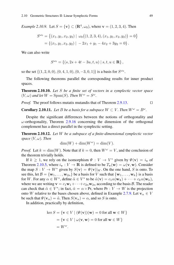
2.10 Geometric Structures II: Linear Symplectic Forms 49
Example 2.10.9. Let S = {v} ⊂ (R4, ω0), where v = (1, 2, 3, 4). Then
Sω0 ={(x1, y1, x2, y2) | ω0
((1, 2, 3, 4), (x1, y1, x2, y2)
)= 0
}
= {(x1, y1, x2, y2) | − 2x1 + y1 − 4x2 + 3y2 = 0} .
We can also write
Sω0 = {(s, 2s+ 4t− 3u, t, u) | s, t, u ∈ R} ,
so the set {(1, 2, 0, 0), (0, 4, 1, 0), (0,−3, 0, 1)} is a basis for Sω0 .
The following theorems parallel the corresponding results for inner productspaces.
Theorem 2.10.10. Let S be a finite set of vectors in a symplectic vector space(V, ω) and let W = Span(S). Then Wω = Sω.
Proof. The proof follows mutatis mutandis that of Theorem 2.9.13. ��Corollary 2.10.11. Let B be a basis for a subspace W ⊂ V . Then Wω = Bω.
Despite the significant differences between the notions of orthogonality andω-orthogonality, Theorem 2.9.16 concerning the dimension of the orthogonalcomplement has a direct parallel in the symplectic setting.
Theorem 2.10.12. Let W be a subspace of a finite-dimensional symplectic vectorspace (V, ω). Then
dim(W ) + dim(Wω) = dim(V ).
Proof. Let k = dim(W ). Note that if k = 0, then Wω = V , and the conclusion ofthe theorem trivially holds.
If k ≥ 1, we rely on the isomorphism Ψ : V → V ∗ given by Ψ(v) = iv ofTheorem 2.10.5, where iv : V → R is defined to be Tv(w) = ω(v,w). Considerthe map S : V → W ∗ given by S(v) = Ψ(v)|W . On the one hand, S is onto. Tosee this, let B = {w1, . . . ,w2n} be a basis for V such that {w1, . . . ,wk} is a basisfor W . For any α ∈ W ∗, define α ∈ V ∗ to be α(v) = c1α(w1) + · · ·+ ckα(wk),where we are writing v = c1w1+ · · ·+c2nw2n according to the basis B. The readercan check that α ∈ V ∗; in fact, α = α ◦ Pr, where Pr : V → W is the projectiononto W relative to the bases chosen above, defined in Example 2.7.9. Let vα ∈ Vbe such that Ψ(vα) = α. Then S(vα) = α, and so S is onto.
In addition, practically by definition,
kerS = {v ∈ V | (Ψ(v))(w) = 0 for all w ∈ W}= {v ∈ V | ω(v,w) = 0 for all w ∈ W}= Wω.
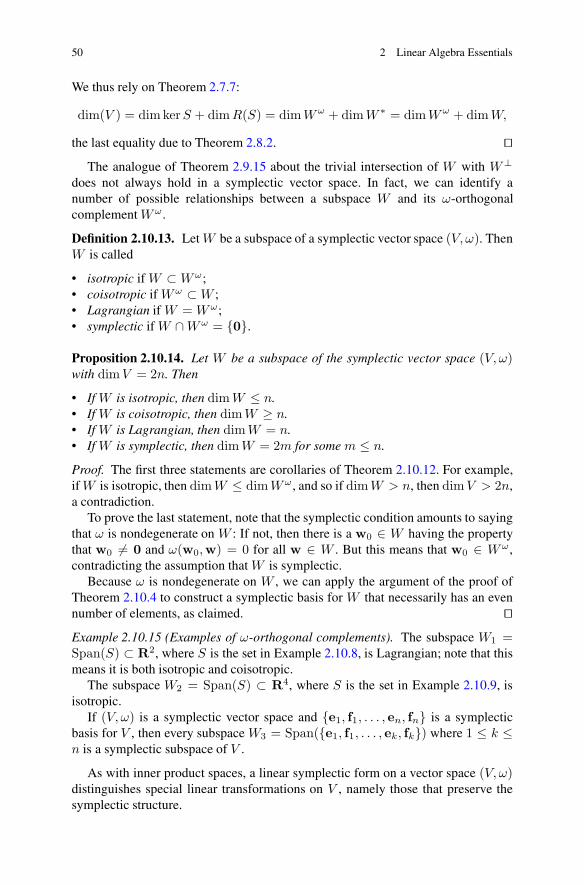
50 2 Linear Algebra Essentials
We thus rely on Theorem 2.7.7:
dim(V ) = dimkerS + dimR(S) = dimWω + dimW ∗ = dimWω + dimW,
the last equality due to Theorem 2.8.2. ��The analogue of Theorem 2.9.15 about the trivial intersection of W with W⊥
does not always hold in a symplectic vector space. In fact, we can identify anumber of possible relationships between a subspace W and its ω-orthogonalcomplement Wω.
Definition 2.10.13. Let W be a subspace of a symplectic vector space (V, ω). ThenW is called
• isotropic if W ⊂ Wω;• coisotropic if Wω ⊂ W ;• Lagrangian if W = Wω;• symplectic if W ∩Wω = {0}.
Proposition 2.10.14. Let W be a subspace of the symplectic vector space (V, ω)with dimV = 2n. Then
• If W is isotropic, then dimW ≤ n.• If W is coisotropic, then dimW ≥ n.• If W is Lagrangian, then dimW = n.• If W is symplectic, then dimW = 2m for some m ≤ n.
Proof. The first three statements are corollaries of Theorem 2.10.12. For example,if W is isotropic, then dimW ≤ dimWω, and so if dimW > n, then dimV > 2n,a contradiction.
To prove the last statement, note that the symplectic condition amounts to sayingthat ω is nondegenerate on W : If not, then there is a w0 ∈ W having the propertythat w0 �= 0 and ω(w0,w) = 0 for all w ∈ W . But this means that w0 ∈ Wω,contradicting the assumption that W is symplectic.
Because ω is nondegenerate on W , we can apply the argument of the proof ofTheorem 2.10.4 to construct a symplectic basis for W that necessarily has an evennumber of elements, as claimed. ��Example 2.10.15 (Examples of ω-orthogonal complements). The subspace W1 =Span(S) ⊂ R2, where S is the set in Example 2.10.8, is Lagrangian; note that thismeans it is both isotropic and coisotropic.
The subspace W2 = Span(S) ⊂ R4, where S is the set in Example 2.10.9, isisotropic.
If (V, ω) is a symplectic vector space and {e1, f1, . . . , en, fn} is a symplecticbasis for V , then every subspace W3 = Span({e1, f1, . . . , ek, fk}) where 1 ≤ k ≤n is a symplectic subspace of V .
As with inner product spaces, a linear symplectic form on a vector space (V, ω)distinguishes special linear transformations on V , namely those that preserve thesymplectic structure.

2.10 Geometric Structures II: Linear Symplectic Forms 51
Definition 2.10.16. Let (V, ω) be a symplectic vector space. A linear transfor-mation T : V → V is a linear symplectomorphism (or a linear symplectictransformation) if for all v,w ∈ V we have ω(T (v), T (w)) = ω(v,w). In thelanguage of Sect. 2.8, T is a linear symplectomorphism if T ∗ω = ω.
We list here some basic properties of linear symplectomorphisms.
Proposition 2.10.17. Let (V, ω) be a finite-dimensional symplectic vector space.Then:
• If T1, T2 : V → V are linear symplectomorphisms, then T2 ◦ T1 is also a linearsymplectomorphism.
• If T : V → V is a linear symplectomorphism, then T has an inverse T−1.Moreover, T−1 is a linear symplectomorphism.
Proof. The reader should refer to Proposition 2.8.16 on the pullback of thecomposition of linear maps.
The first statement follows immediately from the fact that
(T2 ◦ T1)∗ω = T ∗
1 (T∗2 ω).
To prove the second statement, we will show that ker(T ) = {0}; by Theo-rem 2.7.6, this means that T is one-to-one, and so by Corollary 2.7.11, T is alsoonto.
To do this, suppose v ∈ ker(T ) and assume v �= 0. By the nondegeneracyof ω, there exists a vector w such that ω(v,w) �= 0. But since T is a linearsymplectomorphism,
ω(v,w) = (T ∗ω)(v,w)
= ω(T (v), T (w))
= 0 since v ∈ kerT ,
a contradiction. Hence ker(T ) = {0}, proving the claim. So T is invertible withinverse T−1. That T−1 is itself a linear symplectomorphism follows from the factthat
ω = (Id)∗ω = (T ◦ T−1)∗ω = (T−1)∗(T ∗ω) = (T−1)∗ω,
assuming that T is a linear symplectomorphism. ��Linear symplectomorphisms can be characterized in terms of the concept of a
symplectic basis.
Theorem 2.10.18. Let (V, ω) be a symplectic vector space with dimensiondimV = 2n and symplectic basis {e1, f1, . . . , en, fn}. If T : V → V is alinear symplectomorphism, then
{T (e1), T (f1), . . . , T (en), T (fn)}is also a symplectic basis for V .

52 2 Linear Algebra Essentials
Conversely, suppose that
B = {e1, f1, . . . , en, fn}
andB′ = {u1,v1, . . . ,un,vn}
are two symplectic bases for (V, ω) and T : V → V is the linear isomorphismdefined (according to Theorem 2.6.2) by T (ei) = ui and T (fi) = vi. Then T is alinear symplectomorphism.
Proof. The first statement follows from the fact that
ω(T (v), T (w)) = (T ∗ω)(v,w) = ω(v,w),
assuming that T is a linear symplectomorphism.To prove the converse, note that if vectors v and w are written according to the
symplectic basis B, i.e.,
v =∑
(siei + tifi), w =∑
(aiei + bifi),
then a calculation shows that
ω(v,w) =∑
(sibi − tiai).
This calculation holds for any symplectic basis. In particular, we have
(T ∗ω)(v,w) = ω(T (v), T (w)) =∑
(sibi − tiai) = ω(v,w). ��
Proposition 2.10.19. If T is a linear symplectomorphism of (V, ω) and v,w areω-orthogonal, then so are T (v), T (w).
Proof. Exercise. ��We turn now to the matrix representation of the standard symplectic form ω0 on
R2n. This case in fact covers the matrix representation for any linear symplecticform on a symplectic vector space (V, ω), as long as vectors are represented incomponents relative to a symplectic basis.
Recall that the standard symplectic basis B0 for (R2n, ω0) was described above,following Theorem 2.10.4. Writing vectors v,w as column vectors relative to B0,the reader can verify using Proposition 2.8.14 that
ω0(v,w) = wTJv,
where, using block matrix notation,

2.10 Geometric Structures II: Linear Symplectic Forms 53
J =
⎡
⎢⎢⎢⎣
J0 O · · · OO J0 · · · OO O
. . . O
O · · · O J0
⎤
⎥⎥⎥⎦, J0 =
[0 −1
1 0
]
.
The matrix J , representing the standard symplectic form, also allows a matrixcharacterization of a linear symplectomorphism.
Theorem 2.10.20. Let T : R2n → R2n be a linear transformation. Then T isa linear symplectomorphism of (R2n, ω0) if and only if its matrix representationA = [T ] relative to the standard symplectic basis satisfies
AT JA = J.
Proof. The condition that T ∗ω0 = ω0 means that for all v,w ∈ R2n, ω0(T (v),T (w)) = ω0(v,w). But, in matrix notation,
ω0(T (v), T (w)) = (Aw)T J(Av) = wT (AT JA)v,
while ω0(v,w) = wT Jv. Hence T ∗ω0 = ω0 is equivalent to the matrix equationATJA = J . ��
A 2n × 2n matrix satisfying the condition that AT JA = J will be called asymplectic matrix. We write Sp(2n) to denote the set of all 2n × 2n symplecticmatrices. A number of properties of symplectic matrices will be explored in theexercises. The following theorem indicates only the most important properties.
Theorem 2.10.21. Let A ∈ Sp(2n). Then:
1. A is invertible;2. AT ∈ Sp(2n);3. A−1 ∈ Sp(2n).
Proof. In light of Theorem 2.10.20, statements (1) and (3) are in fact corollariesof Proposition 2.10.17. However, we prove the statements here using matrixtechniques.
Suppose A ∈ Sp(2n), i.e., AT JA = J . Then since detJ = 1, we have
1 = det J
= det(AT JA)
= (detA)2,
and so detA = ±1 �= 0. Hence A is invertible.Since J−1 = −J and J2 = −I , and using the fact that ATJA = J , we have
JATJA = J2 = −I,
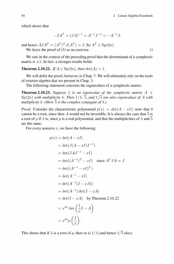
54 2 Linear Algebra Essentials
which shows that
−JAT = (JA)−1 = A−1J−1 = −A−1J,
and hence AJAT = (AT )T J(AT ) = J . So AT ∈ Sp(2n).We leave the proof of (3) as an exercise. ��We saw in the context of the preceding proof that the determinant of a symplectic
matrix is ±1. In fact, a stronger results holds.
Theorem 2.10.22. If A ∈ Sp(2n), then det(A) = 1.
We will defer the proof, however, to Chap. 7. We will ultimately rely on the toolsof exterior algebra that we present in Chap. 3.
The following statement concerns the eigenvalues of a symplectic matrix.
Theorem 2.10.23. Suppose λ is an eigenvalue of the symplectic matrix A ∈Sp(2n) with multiplicity k. Then 1/λ, λ, and 1/λ are also eigenvalues of A withmultiplicity k. (Here λ is the complex conjugate of λ.)
Proof. Consider the characteristic polynomial p(x) = det(A − xI); note that 0cannot be a root, since then A would not be invertible. It is always the case that λ isa root of p if λ is, since p is a real polynomial, and that the multiplicities of λ and λare the same.
For every nonzero x, we have the following:
p(x) = det(A− xI)
= det(J(A − xI)J−1)
= det(JAJ−1 − xI)
= det((A−1)T − xI) since AT JA = J
= det((A−1 − xI)T )
= det(A−1 − xI)
= det(A−1(I − xA))
= det(A−1) det(I − xA)
= det(I − xA) by Theorem 2.10.22
= x2n det
(1
xI −A
)
= x2np
(1
x
)
.
This shows that if λ is a root of p, then so is 1/λ (and hence 1/λ also).
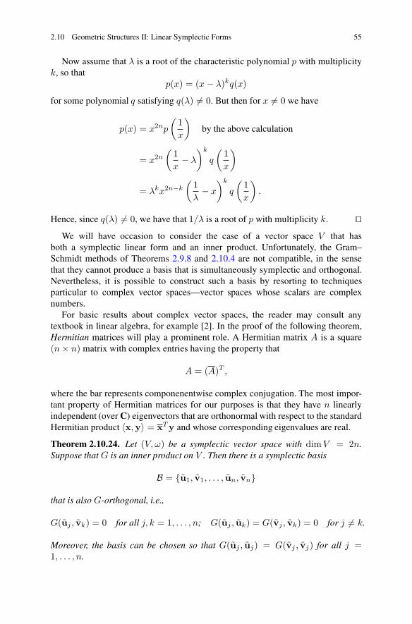
2.10 Geometric Structures II: Linear Symplectic Forms 55
Now assume that λ is a root of the characteristic polynomial p with multiplicityk, so that
p(x) = (x− λ)kq(x)
for some polynomial q satisfying q(λ) �= 0. But then for x �= 0 we have
p(x) = x2np
(1
x
)
by the above calculation
= x2n
(1
x− λ
)k
q
(1
x
)
= λkx2n−k
(1
λ− x
)k
q
(1
x
)
.
Hence, since q(λ) �= 0, we have that 1/λ is a root of p with multiplicity k. ��We will have occasion to consider the case of a vector space V that has
both a symplectic linear form and an inner product. Unfortunately, the Gram–Schmidt methods of Theorems 2.9.8 and 2.10.4 are not compatible, in the sensethat they cannot produce a basis that is simultaneously symplectic and orthogonal.Nevertheless, it is possible to construct such a basis by resorting to techniquesparticular to complex vector spaces—vector spaces whose scalars are complexnumbers.
For basic results about complex vector spaces, the reader may consult anytextbook in linear algebra, for example [2]. In the proof of the following theorem,Hermitian matrices will play a prominent role. A Hermitian matrix A is a square(n× n) matrix with complex entries having the property that
A = (A)T ,
where the bar represents componenentwise complex conjugation. The most impor-tant property of Hermitian matrices for our purposes is that they have n linearlyindependent (over C) eigenvectors that are orthonormal with respect to the standardHermitian product 〈x,y〉 = xTy and whose corresponding eigenvalues are real.
Theorem 2.10.24. Let (V, ω) be a symplectic vector space with dimV = 2n.Suppose that G is an inner product on V . Then there is a symplectic basis
B = {u1, v1, . . . , un, vn}
that is also G-orthogonal, i.e.,
G(uj , vk) = 0 for all j, k = 1, . . . , n; G(uj , uk) = G(vj , vk) = 0 for j �= k.
Moreover, the basis can be chosen so that G(uj , uj) = G(vj , vj) for all j =1, . . . , n.

56 2 Linear Algebra Essentials
Proof. We begin with an orthonormal basis
B′ = {e1, . . . , e2n}
of V relative to G, which exists according to Theorem 2.9.8. Let A be the 2n× 2nmatrix defined by the symplectic form ω relative to B′ as follows:
ω(v,w) = G(v, Aw)
for all v,w ∈ V . We write A = [ajk], where ajk = ω(ej , ek). Due to the skew-symmetry of ω, the matrix A is skew-symmetric: AT = −A.
Throughout this proof, we will consider vectors v,w to be column vectorswritten using components relative to the basis B′. In particular,
G(v,w) = vTw,
and ω(v,w) = vTAw.The skew-symmetry of A implies that the 2n × 2n matrix iA with purely
imaginary entries iajk is Hermitian:
(iA
)T= (−iA)
T since the entries of iA are purely imaginary
= −iAT
= −i(−A) since A is skew-symmetric
= iA.
Since ω is nondegenerate, A must be invertible, and hence the eigenvalues of Aare nonzero. By the property of Hermitian matrices mentioned above, there are infact 2n linearly independent eigenvectors of iA that are orthonormal with respect tothe Hermitian product and with real corresponding eigenvalues. In fact, the readercan verify that the eigenvectors of iA occur in pairs
y1,y1, . . . ,yn,yn
(these are vectors with complex components, and the bar represents componenent-wise complex conjugation). The corresponding eigenvalues will be denoted by
μ1,−μ1, . . . , μn,−μn.
The orthonormality is expressed in matrix notation as
yTj yk = δjk =
{1, j = k,
0, j �= k.

2.10 Geometric Structures II: Linear Symplectic Forms 57
Note that since (iA)yj = μjyj , we have Ayj = (−iμj)yj ; in other words,the eigenvalues of A are ±iμj . For each j = 1, . . . , n, we choose pairs λj andxj as follows: From each pair of eigenvectors yj ,yj with corresponding nonzeroeigenvalues μj ,−μj , choose λj = ±μj so that λj > 0, and then if λj = μj , choosexj = yj , while if λj = −μj , choose xj = yj . In this way, we have Axj = iλjxj
with λj > 0.Write
xj = uj + ivj
with vectors uj and vj having have real components. We claim that the set B′′ ={u1,v1, . . . ,un,vn} is a G-orthogonal basis for V . The fact that B′′ is a basis for Vis a consequence of the above-mentioned property of the eigenvectors of a Hermitianmatrix. To show that B′′ is G-orthogonal, we note that the Hermitian orthonormalitycondition xT
j xk = δjk can be expressed as
uTj uk + vT
j vk = δjk, uTj vk − vT
j uk = 0.
Also, the fact that Axj = iλjxj means that
Auj = −λjvj , Avj = λjuj .
Hence, for j �= k, we have
uTj uk = uT
j
(1
λkAvk
)
=1
λk
(uTj Avk
)Tsince the quantity in parentheses is a scalar
=1
λk
(vTk A
Tuj
)
= − 1
λk
(vTk Auj
)since A is skew-symmetric
=λj
λk
(vTk vj
)since Auj = −λjvj
= −λj
λkuTk uj since uT
j uk + vTj vk = 0 for j �= k
= −λj
λk(uT
k uj)T since the quantity in parentheses is a scalar
= −λj
λkuTj uk,
which implies, since λj , λk > 0, that uTj uk = 0.
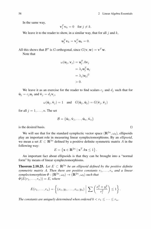
58 2 Linear Algebra Essentials
In the same way,vTj vk = 0 for j �= k.
We leave it to the reader to show, in a similar way, that for all j and k,
uTj vk = vT
j uk = 0.
All this shows that B′′ is G-orthogonal, since G(v,w) = vTw.Note that
ω(uj ,vj) = uTj Avj
= λjuTj uj
= λj |uj |2
> 0.
We leave it as an exercise for the reader to find scalars cj and dj such that foruj = cjuj and vj = djvj ,
ω(uj , vj) = 1 and G(uj , uj) = G(vj , vj)
for all j = 1, . . . , n. The set
B = {u1, v1, . . . , un, vn}
is the desired basis. ��We will see that for the standard symplectic vector space (R2n, ω0), ellipsoids
play an important role in measuring linear symplectomorphisms. By an ellipsoid,we mean a set E ⊂ R2n defined by a positive definite symmetric matrix A in thefollowing way:
E ={x ∈ R2n | xTAx ≤ 1
}.
An important fact about ellipsoids is that they can be brought into a “normalform” by means of linear symplectomorphisms.
Theorem 2.10.25. Let E ⊂ R2n be an ellipsoid defined by the positive definitesymmetric matrix A. Then there are positive constants r1, . . . , rn and a linearsymplectomorphism Φ : (R2n, ω0) → (R2n, ω0) such thatΦ(E(r1, . . . , rn)) = E, where
E(r1, . . . , rn) =
{
(x1, y1, . . . , xn, yn)
∣∣∣∣
∑(x2i + y2ir2i
)
≤ 1
}
.
The constants are uniquely determined when ordered 0 < r1 ≤ · · · ≤ rn.
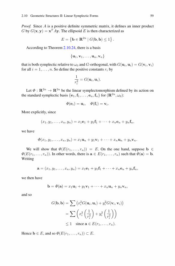
2.10 Geometric Structures II: Linear Symplectic Forms 59
Proof. Since A is a positive definite symmetric matrix, it defines an inner productG by G(x,y) = xTAy. The ellipsoid E is then characterized as
E ={b ∈ R2n | G(b,b) ≤ 1
}.
According to Theorem 2.10.24, there is a basis
{u1,v1, . . . ,un,vn}that is both symplectic relative to ω0 and G-orthogonal, with G(ui,ui) = G(vi,vi)for all i = 1, . . . , n. So define the positive constants ri by
1
r2i= G(ui,ui).
Let Φ : R2n → R2n be the linear symplectomorphism defined by its action onthe standard symplectic basis {e1, f1, . . . , en, fn} for (R2n, ω0):
Φ(ei) = ui, Φ(fi) = vi.
More explicitly, since
(x1, y1, . . . , xn, yn) = x1e1 + y1f1 + · · ·+ xnen + ynfn,
we have
Φ(x1, y1, . . . , xn, yn) = x1un + y1v1 + · · ·+ xnun + ynvn.
We will show that Φ(E(r1, . . . , rn)) = E. On the one hand, suppose b ∈Φ(E(r1, . . . , rn)). In other words, there is a ∈ E(r1, . . . , rn) such that Φ(a) = b.Writing
a = (x1, y1, . . . , xn, yn) = x1e1 + y1f1 + · · ·+ xnen + ynfn,
we then have
b = Φ(a) = x1u1 + y1v1 + · · ·+ xnun + ynvn,
and so
G(b,b) =∑(
x2iG(ui,ui) + y2iG(vi,vi)
)
=∑
(
x2i
(1
r2i
)
+ y2i
(1
r2i
))
≤ 1 since a ∈ E(r1, . . . , rn).
Hence b ∈ E, and so Φ(E(r1, . . . , rn)) ⊂ E.

60 2 Linear Algebra Essentials
On the other hand, suppose that b ∈ E, so that G(b,b) ≤ 1. There is a ∈ R2n
such that Φ(a) = b, since Φ is a linear isomorphism. Writing b according to thebasis above, we obtain
b = x1u1 + y1v1 + · · ·+ xnun + ynvn,
soa = (x1, y1, . . . , xn, yn).
But∑
(x2i + y2ir2i
)
= G(b,b) ≤ 1,
and so a ∈ E(r1, . . . , rn) and E ⊂ Φ(E(r1, . . . , rn)).All this shows that Φ(E(r1, . . . , rn)) = E.To show that the constants ri are uniquely determined up to ordering, suppose
that there are linear symplectomorphisms Φ1, Φ2 : R2n → R2n and n-tuples(r1, . . . , rn), (r′1, . . . , r
′n) with 0 < r1 ≤ · · · ≤ rn and 0 < r′1 ≤ · · · ≤ r′n
such thatΦ1(E(r1, . . . , rn)) = E, Φ2(E(r′1, . . . , r
′n)) = E.
Then, writing Φ = Φ−11 ◦ Φ2, we have
Φ(E(r′1, . . . , r′n)) = E(r1, . . . , rn).
In matrix notation, this says that xTD′x ≤ 1 if and only if (Φx)TD(Φx) =xT (ΦTDΦ)x ≤ 1, where x = (x1, y1, . . . , xn, yn) is a column vector, D is thediagonal matrix D = diag
[1/(r1)
2, 1/(r1)2, . . . , 1/(rn)
2, 1/(rn)2], and D′ is the
diagonal matrix D′ = diag[1/(r′1)
2, 1/(r′1)2, . . . , 1/(r′n)
2, 1/(r′n)2]. This implies
thatΦTDΦ = D′.
The facts that Φ satisfies ΦT JΦ = J and J−1 = −J together imply ΦT =−JΦ−1J , and so
Φ−1JDΦ = JD′.
This shows that JD is similar to JD′, and so the two matrices have the sameeigenvalues. The reader may verify that the eigenvalues of JD are ±irj and thoseof JD′ are ±ir′j . Since the ri and r′i are ordered from least to greatest, we musthave rj = r′j for all j = 1, . . . , n. ��
Theorem 2.10.25 prompts the following definition.
Definition 2.10.26. Let E ⊂ R2n be an ellipsoid in the standard symplecticspace (R2n, ω0). The symplectic spectrum of E is the unique n-tuple σ(E) =(r1, . . . , rn), 0 < r1 ≤ · · · ≤ rn, such that there is a linear symplectomorphismΦ with Φ(E(r1, . . . , rn)) = E (Fig. 2.6).

2.12 Exercises 61
Ψ−1
(x2, y2)
(x1, y1)
(x2, y2)
(x1, y1)−r1 r1
r2
−r2
E
σ(E)=(r1, r2)
E(r1, r2)
Fig. 2.6 Linear symplectomorphisms and the symplectic spectrum.
We will continue to develop some topics in linear symplectic geometry inSect. 7.7 as motivation for a key concept in (nonlinear) symplectic geometry, thesymplectic capacity.
2.11 For Further Reading
With the exception of Sects. 2.8 and 2.10, much of the material in this chapter canbe found in any textbook on linear algebra. The notation here generally follows thatin [2].
While many linear algebra textbooks have detailed presentations of inner productspaces, symplectic vector spaces are usually presented only as introductory matterin the context of specialized texts. We refer to A. Banyaga’s summary in [4, Chap. 1]or to [31].
2.12 Exercises
The exercises in this chapter emphasize topics not usually presented in a firstelementary linear algebra course.
2.1. Prove Theorem 2.4.3.
2.2. Prove Theorem 2.4.10.
2.3. Prove Theorem 2.4.13.
2.4. Let T : V → W be a linear isomorphism between vector spaces V and W , andlet T−1 : W → V be the inverse of T . Show that T−1 is a linear transformation.
2.5. Consider the basis B = {b1,b2,b3} of R3, where
62 2 Linear Algebra Essentials
b1 = (1, 0, 1), b2 = (1, 1, 0), b3 = (0, 2, 1).
(a) Write the components of w = (2, 3, 5) relative to the basis B.(b) Let {β1, β2, β3} be the basis of (R3)∗ dual to B. Compute βi(w) for each
i = 1, 2, 3, where w is the vector given in part (a).(c) For each i = 1, 2, 3, compute βi(v), where v = (v1, v2, v3) is an arbitrary
vector in R3.
2.6. For each of the linear transformations Ψ and linear one-forms T below,compute Ψ∗T :
(a) Ψ : R3 → R3, Ψ(u, v, w) = (2u, 3u− v − w, u+ 2w),
T (x, y, z) = 3x+ y − z.
(b) Ψ : R3 → R2, Ψ(u, v, w) = (v, 2u− w),
T (x, y) = x+ 3y.
(c) Ψ : R4 → R3, Ψ(x, y, z, w) = (x+ y − z − 2w,w − 4x− z, y + 3z),
T (x, y, z) = x− 2y + 3z.
2.7. Let α ∈ (R3)∗ be given by α(x, y, z) = 4y + z.
(a) Find kerα.(b) Find all linear transformations Ψ : R3 → R3 with the property that Ψ∗α = α.
2.8. Consider the linear transformation T : R2 → R2 given by T (x1, x2) =(2x1 − x2, x1 + 3x2).
(a) Compute T ∗G0, where G0 is the standard inner product defined in Exam-ple 2.8.11.
(b) Compute T ∗S, where S is the bilinear form in Example 2.8.13.
2.9. Let T : Rn → Rn be a linear transformation described in matrix form [T ]relative to the standard basis for Rn. Show that for every n× n matrix A, one has
T ∗GA = GA[T ],
where GA and GA[T ] are defined according to Example 2.8.12.
2.10. Prove the following converse to Proposition 2.8.14: Let B be an n×n matrixand let E be a basis for the n-dimensional vector space V . Then the function b :V × V → R defined by
b(v,w) = wTBv,
where v and w are written as column vectors relative to the basis E , is a bilinearform.
2.12 Exercises 63
2.11. Use Exercise 2.10 to give five examples of bilinear forms on R3 and fiveexamples of bilinear forms on R4.
2.12. Let b, B, and E be as given in Exercise 2.10, and let T : V → V be a lineartransformation. Show that T ∗b = b, where b is the bilinear form corresponding tothe matrix ATBA for A = [T ]E,E , the matrix representation of T relative to thebasis E .
2.13. For each of the following 2× 2 matrices, write the coordinate expression forthe inner product GA relative to the standard basis as in Example 2.9.4. For each,compute GA(e1, e1), GA(e1, e2), and GA(e2, e2) along with ∠(e1, e2), wheree1 = (1, 0) and e2 = (0, 1):
(a)
[2 1
1 − 1
]
;
(b)
[2 − 1
1 3
]
;
(c)
[1 2
1 3
]
.
2.14. Show that the function G(v,w) = v1w1 + 2v1w2 + 2v2w1 + 5v2w2 is aninner product on R2, where v = (v1, v2) and w = (w1, w2). Find an orthonormalbasis {u1,u2} for R2 relative to G.
2.15. Let {u1,u2} be the basis for R2 given by u1 = (3, 2) and u2 = (1, 1). Let Gbe the inner product on R2 such that {u1,u2} is orthonormal (see Theorem 2.9.9).Find G(v,w), where v = (v1, v2) and w = (w1, w2). Find ∠((1, 0), (0, 1)).2.16. Prove Theorem 2.9.10.
2.17. For the following subspaces W of Rn, find a basis for W⊥, the orthogonalcomplement of W relative to the standard inner product on Rn
(a) W = Span {(1, 2)} ⊂ R2;(b) W = Span {(1, 2, 3)} ⊂ R3;(c) W = Span {(1, 0, 1), (−1, 1, 0)} ⊂ R3;(d) W = Span {(1,−2, 2, 1), (0, 1, 1,−3)} ⊂ R4.
2.18. Provide the details for the proof of Theorem 2.9.16.
2.19. Let (V,G) be an inner product space and let W be a subset of V .
(a) Show that W ⊂ (W⊥)⊥.(b) Show that if V is finite-dimensional, then there is an orthonormal basis
{u1, . . . ,un} of V such that {u1, . . . ,uk} is a basis forW and {uk+1, . . . ,un}is a basis for W⊥. (See Theorem 2.9.16.)
(c) Show that if V is finite-dimensional, then (W⊥)⊥ ⊂ W , and so by (a), W =(W⊥)⊥.
2.20. Prove Proposition 2.9.18.
64 2 Linear Algebra Essentials
2.21. Prove Proposition 2.9.21.
2.22. Let (V,G) be a finite-dimensional inner product space. Show that a lineartransformation T : V → V is a linear isometry if and only if for every orthonormalbasis {e1, . . . , en} of V , the set {T (e1), . . . , T (en)} is also an orthonormal basisfor V .
2.23. Give three examples of linear symplectic forms on R4.
2.24. Suppose B = {a1,b1, . . . , an,bn} is a basis for R2n. Define the alternatingbilinear form ωB by specifying its action on the basis vectors,
ωB(ai, aj) = ωB(bi,bj) = 0 for all i, j,
ωB(ai,bj) = 0 for i �= j,
ωB(ai,bi) = 1,
and extending bilinearly. Show that ωB is a linear symplectic form.
2.25. Define a bilinear form S on R4 by S(v,w) = wTAv, where
A =
⎡
⎢⎢⎣
0 1 1 1
−1 0 2 0
−1 − 2 0 3
−1 0 − 3 0
⎤
⎥⎥⎦ .
(a) Show that S is a linear symplectic form.(b) Use the process outlined in Theorem 2.10.4 to find a symplectic basis
{e1, f1, e2, f2} for R4 relative to S.
2.26. Use the procedure in Theorem 2.10.4 to construct three different symplecticbases for R4 by making appropriate choices at different stages of the process.
2.27. Consider (R4, ω0), where ω0 is the standard linear symplectic form onR4. Decide whether the following subspaces of R4 are isotropic, coisotropic,Lagrangian, or symplectic:
(a) W1 = Span {(1, 0,−1, 3)};(b) W2 = Span {(3, 1, 0,−1), (2, 1, 2, 1)};(c) W3 = Span {(1, 0, 2,−1), (0, 1, 1,−1)};(d) W4 = Span {(1, 1, 1, 0), (2,−1, 0, 1), (0, 2, 0,−1)};(e) W5 = kerT , where T : R4 → R2 is given by
T (x1, y1, x2, y2) = (2x2 − y1, x1 + x2 + y1 + y2).
2.28. Prove Theorem 2.10.7.
2.29. Prove Theorem 2.10.12.

2.12 Exercises 65
2.30. Let W1 and W2 be subspaces of a symplectic vector space (V, ω). Show thatif W1 ⊂ W2, then (W2)
ω ⊂ (W1)ω .
2.31. Show that if W is a subspace of a finite-dimensional symplectic vector space(V, ω), then (Wω)ω = W . (See Exercise 2.19.)
2.32. Is it possible for a 2-dimensional subspace of a 4-dimensional symplecticvector space to be neither symplectic nor Lagrangian? If so, find necessaryconditions for this to occur. If not, state and prove the corresponding result. To whatextent can this question be generalized to higher dimensions?
2.33. Prove Proposition 2.10.19.
2.34. Prove Theorem 2.10.5.
2.35. For each of the examples in Exercise 2.23, write the isomorphismΨ describedin Theorem 2.10.5 explicitly in terms of the standard bases of R4 and (R4)∗.
2.36. Let W be a subspace of a finite-dimensional symplectic vector space (V, ω).Let Ψ : V → V ∗ be the isomorphism described in Theorem 2.10.5.
(a) LetW 0 = {α ∈ V ∗ | α(w) = 0 for all w ∈ W} .
Show that W 0 is a subspace of V ∗.(b) Show that Ψ(Wω) = W 0.(c) Show that Ψ(W ) = (Wω)0.
2.37. Provide the details for the proof of Theorem 2.10.24. In particular:
(a) Show that the set B′′ is a basis for V .(b) Show that uT
j vk = vTj uk = 0.
(c) Find scalars cj and dj such that for uj = cjuj and vj = djvj ,
ω(uj , vj) = 1 and G(uj , uj) = G(vj , vj)
for all j = 1, . . . , n.
2.38. Verify directly that the matrix
A =
⎡
⎢⎢⎣
1 − 1 1 0
1 − 1 0 1
1 − 1 0 0
2 − 1 1 − 1
⎤
⎥⎥⎦
is a symplectic matrix, i.e., that ATJA = J .
2.39. Let B = {a1,b1, . . . , an,bn} be a symplectic basis for the standardsymplectic space (R2n, ω0). Show that the matrix

66 2 Linear Algebra Essentials
A =[a1 b1 · · · an bn
]
is a symplectic matrix.
2.40. Show that if A ∈ Sp(2n), then A−1 ∈ Sp(2n).
2.41. Show that if A ∈ Sp(2n), then A−1 = −JAT J .

http://www.springer.com/978-1-4614-7731-0