LINEAR ALGEBRA AND MATRIX METHODS IN ...flash.lakeheadu.ca/~kyu/E5111/Theil1983.pdfI: Linear Algebra...
63
Chapter I LINEAR ALGEBRA AND MATRIX METHODS IN ECONOMETRICS HENRI THEIL* University of Florida Contents 1. Introduction 2. Why are matrix methods useful in econometrics? 2.1. Linear systems and quadratic forms 2.2. Vectors and matrices in statistical theory 2.3. Least squares in the standard linear model 2.4. Vectors and matrices in consumption theory 3. Partitioned matrices 3. I, The algebra of partitioned matrices 3.2. Block-recursive systems 3.3. Income and price derivatives revisited 4. Kronecker products and the vectorization of matrices 4. I. The algebra of Kronecker products 4.2. Joint generalized least-squares estimation of several equations 4.3. Vectorization of matrices 5. Differential demand and supply systems 5.1. A differential consumer demand system 5.2. A comparison with simultaneous equation systems 5.3. An extension to the inputs of a firm: A singularity problem 5.4. A differential input demand system 5.5. Allocation systems 5.6. Extensions 6. Definite and semidefinite square matrices 6. I. Covariance matrices and Gauss-Markov further considered 6.2. Maxima and minima 6.3. Block-diagonal definite matrices 7. Diagonalizations 7.1. ne standard diagonalization of a square matrix 5 : 7 *: :; :: 16 16 17 19 20 ;; 2: 29 30 3”: *Research supported in part by NSF Grant SOC76-82718. The author is indebted to Kenneth Clements (Reserve Bank of Australia, Sydney) and Michael Intriligator (University of California, Los Angeles) for comments on an earlier draft of this chapter. Hundhook of Econometrics, Volume I, Edited by Z. Griliches and M.D. Intriligator 0 North- Holland Publishing Company, I983
Transcript of LINEAR ALGEBRA AND MATRIX METHODS IN ...flash.lakeheadu.ca/~kyu/E5111/Theil1983.pdfI: Linear Algebra...

Chapter I
LINEAR ALGEBRA AND MATRIX METHODS IN ECONOMETRICS
HENRI THEIL*
University of Florida
Contents
1. Introduction 2. Why are matrix methods useful in econometrics?
2.1. Linear systems and quadratic forms 2.2. Vectors and matrices in statistical theory 2.3. Least squares in the standard linear model 2.4. Vectors and matrices in consumption theory
3. Partitioned matrices 3. I, The algebra of partitioned matrices 3.2. Block-recursive systems 3.3. Income and price derivatives revisited
4. Kronecker products and the vectorization of matrices 4. I. The algebra of Kronecker products 4.2. Joint generalized least-squares estimation of several equations 4.3. Vectorization of matrices
5. Differential demand and supply systems 5.1. A differential consumer demand system 5.2. A comparison with simultaneous equation systems 5.3. An extension to the inputs of a firm: A singularity problem 5.4. A differential input demand system 5.5. Allocation systems 5.6. Extensions
6. Definite and semidefinite square matrices 6. I. Covariance matrices and Gauss-Markov further considered 6.2. Maxima and minima 6.3. Block-diagonal definite matrices
7. Diagonalizations 7.1. ne standard diagonalization of a square matrix
5
: 7
*:
:;
:: 16 16 17 19 20
;;
2:
29 30
3”:
*Research supported in part by NSF Grant SOC76-82718. The author is indebted to Kenneth Clements (Reserve Bank of Australia, Sydney) and Michael Intriligator (University of California, Los Angeles) for comments on an earlier draft of this chapter.
Hundhook of Econometrics, Volume I, Edited by Z. Griliches and M.D. Intriligator 0 North- Holland Publishing Company, I983

H. Theil
1.2. Special cases 7.3. Aitken’s theorem 7.4. The Cholesky decomposition 7.5. Vectors written as diagonal matrices 7.6. A simultaneous diagonalization of two square matrices 7.7. Latent roots of an asymmetric matrix
8. Principal components and extensions 8.1. Principal components 8.2. Derivations 8.3. Further discussion of principal components 8.4. The independence transformation in microeconomic theory 8.5. An example 8.6. A principal component interpretation
9. The modeling of a disturbance covariance matrix 9.1. Rational random behavior 9.2. The asymptotics of rational random behavior 9.3. Applications to demand and supply
10. The Moore-Penrose inverse 10.1. Proof of the existence and uniqueness 10.2. Special cases 10.3. A generalization of Aitken’s theorem 10.4. Deleting an equation from an allocation model
Appendix A: Linear independence and related topics Appendix B: The independence transformation Appendix C: Rational random behavior References
:: 53 56 57 58 61 64
Ch. 1: Linear Algebra and Matrix Methoak
1. Introduction
Vectors and matrices played a minor role in the econometric literature published before World War II, but they have become an indispensable tool in the last several decades. Part of this development results from the importance of matrix tools for the statistical component of econometrics; another reason is the in- creased use of matrix algebra in the economic theory underlying econometric relations. The objective of this chapter is to provide a selective survey of both areas. Elementary properties of matrices and determinants are assumed to be known, including summation, multiplication, inversion, and transposition, but the concepts of linear dependence and orthogonality of vectors and the rank of a matrix are briefly reviewed in Appendix A. Reference is made to Dhrymes (1978), Graybill (1969), or Hadley (1961) for elementary properties not covered in this chapter.
Matrices are indicated by boldface italic upper case letters (such as A), column vectors by boldface italic lower case letters (a), and row vectors by boldface italic lower case letters with a prime added (a’) to indicate that they are obtained from the corresponding column vector by transposition. The following abbreviations are used:
LS = least squares,
GLS = generalized least squares,
ML = maximum likelihood,
6ij=Kroneckerdelta(=lifi=j,0ifi*j).
2. Why are matrix methods useful in econometrics?
2.1. Linear systems and quadratic forms
A major reason why matrix methods are useful is that many topics in economet- rics have a multivariate character. For example, consider a system of L simulta- neous linear equations in L endogenous and K exogenous variables. We write y,, and x,~ for the &h observation on the lth endogenous and the kth exogenous variable. Then thejth equation for observation (Y takes the form
k=l
(2.1)
tively:
r YII Y12-.*YIL PI1 Pl2-.-PIL
Y21 Y22...Y2L P 21 P22...P2L r= . . . , B= . . . . . . . . .
YLI YL2.. YLL _P’ P,,...P,L_ KI
When there are n observations ((Y = 1,. . . , n), there are Ln equations of the form (2.1) and n equations of the form (2.2). We can combine these equations compactly into
E=
6 H. Theil
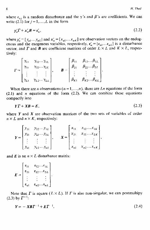
where &aj is a random disturbance and the y’s and p’s are coefficients. We can write (2.1) forj=l,...,L in the form
y;I’+ x&B = E&, (2.2)
whereyL= [yal... yaL] and x& = [ xal . . . xaK] are observation vectors on the endog- enous and the exogenous variables, respectively, E& = [ E,~. . . caL] is a disturbance vector, and r and B are coefficient matrices of order L X L and K X L, respec-
Yr+ XB=E, (2.3)
where Y and X are observation matrices of the two sets of variables of order n X L and n X K, respectively:
Yll Yl,...YlL XII X12...XlK
Y21 Y22 . -Y2 L x21 X22-.-X2K
y= . . . 3 x= . . . 3 . . . . . . . .
_Y nl YtlZ...Y?lL_ X nl xn2.-. nK X
and E is an n X L disturbance matrix:
-%I El2...ElL
E2l E22...&2L
. .
. .
. .
E nl %2... nL E
Note that r is square (L X L). If r is also non-singular, we can postmultipy (2.3) by r-t:
Y= -XBr-'+Er-'. (2.4)

Ch. I: Linear Algebra and Matrix Methods I
This is the reduced form for all n observations on all L endogenous variables, each of which is described linearly in terms of exogenous values and disturbances. By contrast, the equations (2.1) or (2.2) or (2.3) from which (2.4) is derived constitute the structural form of the equation system.
The previous paragraphs illustrate the convenience of matrices for linear systems. However, the expression “linear algebra” should not be interpreted in the sense that matrices are useful for linear systems only. The treatment of quadratic functions can also be simplified by means of matrices. Let g( z,, . . . ,z,) be a three tunes differentiable function. A Taylor expansion yields
dz ,,...,z/J=&,..., Q+ ; (zi-q)z i=l I
+g ; (ZiGi) r=l j=l
&(r,mzj)+03Y (2.5)
where 0, is a third-order remainder term, while the derivatives Jg/azi and a2g/azi dzj are all evaluated at z, = Z,,. . .,zk = I,. We introduce z and Z as vectors with ith elements zi and I~, respectively. Then (2.5) can be written in the more compact form
ag 1 8% g(Z)=g(Z)+(Z-z)‘az+Z(Z-‘)‘azaz, -(z -z)+o,, (2.6)
where the column vector ag/az = [ ag/azi] is the gradient of g( .) at z (the vector of first-order derivatives) and the matrix a*g/az az’ = [ a2g/azi azj] is the Hessian matrix of g( .) at T (the matrix of second-order derivatives). A Hessian matrix is always symmetric when the function is three times differentiable.
2.2. Vectors and matrices in statistical theory
Vectors and matrices are also important in the statistical component of economet- rics. Let r be a column vector consisting of the random variables r,, . . . , r,. The expectation Gr is defined as the column vector of expectations Gr,, . . . , Gr,. Next consider
(r- &r)(r- &r)‘= I r, - Gr, r, - Gr, . I : [rl - Gr, r2 - &r,...r, - Gr,]
8 H. Theil
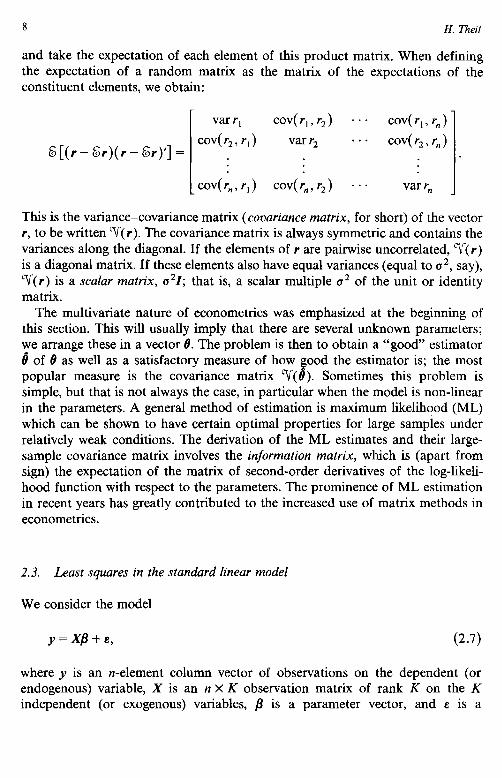
and take the expectation of each element of this product matrix. When defining the expectation of a random matrix as the matrix of the expectations of the constituent elements, we obtain:
&[(r-&r)(r-&r)‘]=
var r, cov(r,,r,) e-e cov( rl , rn )
4 r2, rl ) varr, --- cov( r2, r, >
cov(r,,r,) cov(r,,r2) ... var r,
This is the variance-covariance matrix (covariance matrix, for short) of the vector r, to be written V(r). The covariance matrix is always symmetric and contains the variances along the diagonal. If the elements of r are pairwise uncorrelated, ‘T(r)
is a diagonal matrix. If these elements also have equal variances (equal to u2, say), V(r) is a scalar matrix, a21; that is, a scalar multiple a2 of the unit or identity matrix.
The multivariate nature of econometrics was emphasized at the beginning of this section. This will usually imply that there are several unknown parameters; we arrange these in a vector 8. The problem is then to obtain a “good” estimator 8 of B as well as a satisfactory measure of how good the estimator is; the most popular measure is the covariance matrix V(O). Sometimes this problem is simple, but that is not always the case, in particular when the model is non-linear in the parameters. A general method of estimation is maximum likelihood (ML) which can be shown to have certain optimal properties for large samples under relatively weak conditions. The derivation of the ML estimates and their large- sample covariance matrix involves the information matrix, which is (apart from sign) the expectation of the matrix of second-order derivatives of the log-likeli- hood function with respect to the parameters. The prominence of ML estimation in recent years has greatly contributed to the increased use of matrix methods in econometrics.
2.3. Least squares in the standard linear model
We consider the model
y=Xtl+&, (2.7)
where y is an n-element column vector of observations on the dependent (or endogenous) variable, X is an n X K observation matrix of rank K on the K independent (or exogenous) variables, j3 is a parameter vector, and E is a
Ch. I: Linear Algebra and Matrix Method 9
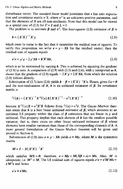
disturbance vector. The standard linear model postulates that E has zero expecta- tion and covariance matrix a*I, where u* is an unknown positive parameter, and that the elements of X are all non-stochastic. Note that this model can be viewed as a special case of (2.3) for r = I and L, = 1.
The problem is to estimate B and u2. The least-squares (LS) estimator of /I is
b = (XX)_‘X’y (2.8)
which owes its name to the fact that it minimizes the residual sum of squares. To verify this proposition we write e = y - Xb for the residual vector; then the residual sum of squares equals
e’e = y’y - 2 y’Xb + b’x’Xb, (2.9)
which is to be minimized by varying 6. This is achieved by equating the gradient of (2.9) to zero. A comparison of (2.9) with (2.5) and (2.6), with z interpreted as b, shows that the gradient of (2.9) equals - 2X’y + 2x’Xb, from which the solution (2.8) follows directly.
Substitution of (2.7) into (2.8) yields b - j3 = (X’X)- ‘X’e. Hence, given &e = 0 and the non-randomness of X, b is an unbiased estimator of /3. Its covariance matrix is
V(b) = (XtX)-‘X’?f(e)X(X’X)-’ = a2(X’X)-’ (2.10)
because X’?f( e)X = a2X’X follows from ?r( e) = a21. The Gauss-Markov theo- rem states that b is a best linear unbiased estimator of /3, which amounts to an optimum LS property within the class of /I estimators that are linear in y and unbiased. This property implies that each element of b has the smallest possible variance; that is, there exists no other linear unbiased estimator of /3 whose elements have smaller variances than those of the corresponding elements of b. A more general formulation of the Gauss-Markov theorem will be given and proved in Section 6.
Substitution of (2.8) into e = y - Xb yields e = My, where M is the symmetric matrix
M=I-X(X/X)_‘X (2.11)
which satisfies MX = 0; therefore, e = My = M(XB + E) = Me. Also, M is idempotent, i.e. M2 = M. The LS residual sum of squares equals e’e = E’M’ME = E’M*E and hence
e’e = E’ME. (2.12)
10 H. Theil
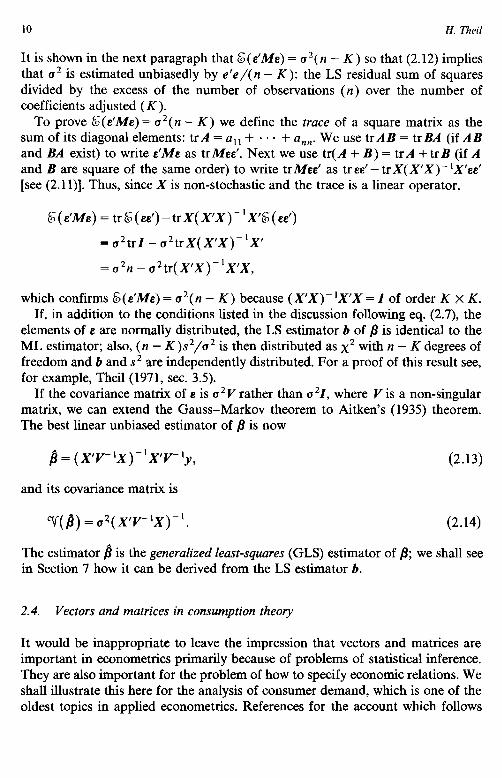
It is shown in the next paragraph that &(e’Me) = a2(n - K) so that (2.12) implies that cr2 is estimated unbiasedly by e’e/(n - K): the LS residual sum of squares divided by the excess of the number of observations (n) over the number of coefficients adjusted (K).
To prove &(&Me) = a2( n - K) we define the truce of a square matrix as the sum of its diagonal elements: trA = a,, + * * - + a,,,,. We use trAB = trBA (if AB and BA exist) to write s’Me as trMee’. Next we use tr(A + B) = trA + trB (if A and B are square of the same order) to write trMee’ as tree’ - trX( X’X)- ‘X’ee’ [see (2.1 l)]. Thus, since X is non-stochastic and the trace is a linear operator,
&(e’Me) = tr&(ee’)-trX(X’X)-‘X’&(ee’)
= a2trl - a2trX(X’X)-‘X’
= u2n - u2tr( X(X)-‘X’X,
which confirms &(e’Me) = a’( n - K) because (X’X)- ‘X’X = I of order K x K. If, in addition to the conditions listed in the discussion following eq. (2.7), the
elements of e are normally distributed, the LS estimator b of /3 is identical to the ML estimator; also, (n - K)s2/u2 is then distributed as x2 with n - K degrees of .freedom and b and s2 are independently distributed. For a proof of this result see, for example, Theil(l971, sec. 3.5).
If the covariance matrix of e is u2V rather than u21, where Y is a non-singular matrix, we can extend the Gauss-Markov theorem to Aitken’s (1935) theorem. The best linear unbiased estimator of /3 is now
fi = (xv-lx)-‘xv-‘y, (2.13)
and its covariance matrix is
V(B) = uqxv-‘x)-l. (2.14)
The estimator fi is the generalized least-squares (GLS) estimator of /3; we shall see in Section 7 how it can be derived from the LS estimator b.
2.4. Vectors and matrices in consumption theory
It would be inappropriate to leave the impression that vectors and matrices are important in econometrics primarily because of problems of statistical inference. They are also important for the problem of how to specify economic relations. We shall illustrate this here for the analysis of consumer demand, which is one of the oldest topics in applied econometrics. References for the account which follows

Ch. I: Linear Algebra and Matrix Methods 11
include Barten (1977) Brown and Deaton (1972) Phlips (1974), Theil(l975-76), and Deaton’s chapter on demand analysis in this Handbook (Chapter 30).
Let there be N goods in the marketplace. We write p = [pi] and q = [ qi] for the price and quantity vectors. The consumer’s preferences are measured by a utility function u(q) which is assumed to be three times differentiable. His problem is to maximize u(q) by varying q subject to the budget constraintsp’q = M, where A4 is the given positive amount of total expenditure (to be called income for brevity’s sake). Prices are also assumed to be positive and given from the consumer’s point of view. Once he has solved this problem, the demand for each good becomes a function of income and prices. What can be said about the derivatives of demand, aqi/ahf and aqi/apj?
Neoclassical consumption theory answers this question by constructing the Lagrangian function u(q)- A( pQ - M) and differentiating this function with respect to the qi’s. When these derivatives are equated to zero, we obtain the familiar proportionality of marginal utilities and prices:
au - = Ap,, aqi i=l,...,N, (2.15)
or, in vector notation, au/l@ = Xp: the gradient of the utility function at the optimal point is proportional to the price vector. The proportionality coefficient X has the interpretation as the marginal utility of income.’
The proportionality (2.15) and the budget constraint pb = A4 provide N + 1 equations in N + 1 unknowns: q and A. Since these equations hold identically in M and p, we can differentiate them with respect to these variables. Differentiation of p@ = M with respect to M yields xi pi( dq,/dM) = 1 or
(2.16)
where */ait = [ dqi/dM] is the vector of income derivatives of demand. Differentiation of pb = A4 with respect to pi yields &pi( aqi/apj)+ qj = 0 (j = 1 ,...,N) or
,a4 P ap’ = -4’9 (2.17)
where aQ/ap’ = [ aqi/apj] is the N X N matrix of price derivatives of demand. Differentiation of (2.15) with respect to A4 and application of the chain rule
‘Dividing both sides of (2.15) by pi yields 8u/6’(piqi) = X, which shows that an extra dollar of income spent on any of the N goods raises utility by h. This provides an intuitive justification for the interpretation. A more rigorous justification would require the introduction of the indirect utility function, which is beyond the scope of this chapter.
12 H. Theil
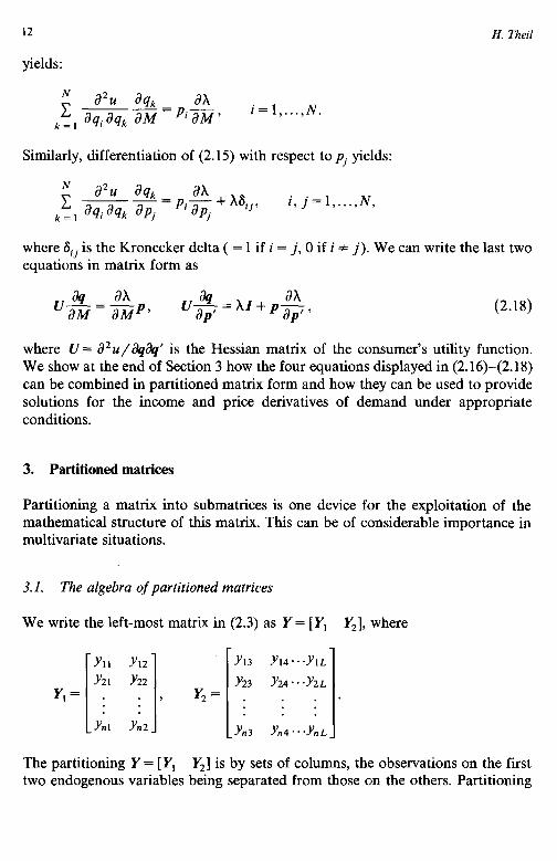
yields:
Similarly, differentiation of (2.15) with respect to pj yields:
kfE,&$=Pi$+xs,/, i,j=l ,.**, N, 1 J J
where aij is the Kronecker delta ( = 1 if i = j, 0 if i * j). We can write the last two equations in matrix form as
(2.18)
where U = a2u/&&’ is the Hessian matrix of the consumer’s utility function. We show at the end of Section 3 how the four equations displayed in (2.16)-(2.18) can be combined in partitioned matrix form and how they can be used to provide solutions for the income and price derivatives of demand under appropriate conditions.
3. Partitioned matrices
Partitioning a matrix into submatrices is one device for the exploitation of the mathematical structure of this matrix. This can be of considerable importance in multivariate situations.
3.1. The algebra of partitioned matrices
We write the left-most matrix in (2.3) as Y = [Y, Y2], where
Y13 Yl,...YlL
Y23 Y24 * * -Y2 L y2= . . . f _: . . . .
Yns Yn4.*.YnL_
The partitioning Y = [Yl Y2] is by sets of columns, the observations on the first two endogenous variables being separated from those on the others. Partitioning
Ch. 1: Linear Algebra and Matrix Methodr 13
may take place by row sets and column sets. The addition rule for matrices can be applied in partitioned form,
provided AI, and Bjj have the same order for each (i, j). A similar result holds for multiplication,
provided that the number of columns of P,, and P2, is equal to the number of rows of Q,, and Q12 (sillily for P12, P22, Q2,, Q&.
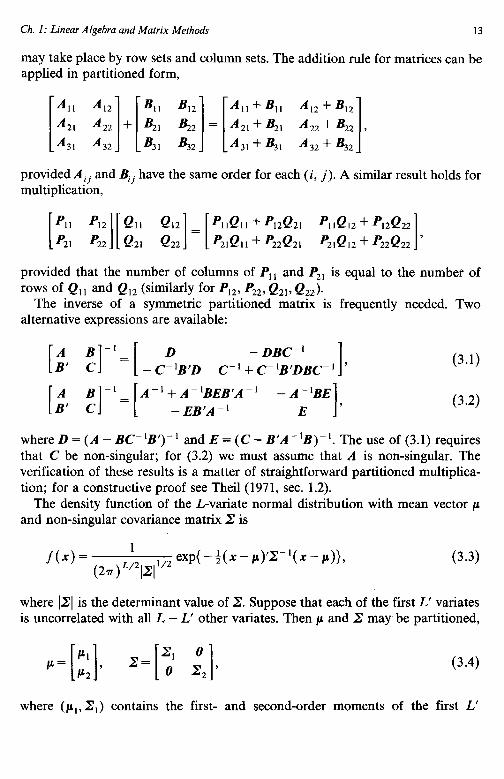
The inverse of a symmetric partitioned matrix is frequently needed. Two alternative expressions are available:
[;’ ;]-I= [ _Cf)‘B’D C-1;$j;;BC-‘1’ (3.1)
[z4, :I-‘= [A-‘+;;yi(-’ -AilBE], (3.2)
where D = (A - BC-‘B’)-’ and E = (C - B’A-‘B)-‘. The use of (3.1) requires that C be non-singular; for (3.2) we must assume that A is non-singular. The verification of these results is a matter of straightforward partitioned multiplica- tion; for a constructive proof see Theil(l971, sec. 1.2).
The density function of the L-variate normal distribution with mean vector p and non-singular covariance matrix X is
f(x)= l (27r) L’2p11’2
exp{-t(x-Cc)‘~-‘(x-Er)), (3.3)
where 1x1 is the determinant value of X. Suppose that each of the first L’ variates is uncorrelated with all L - L’ other variates. Then p and X may be partitioned,
(3.4)
where (p,, Z,) contains the first- and second-order moments of the first L’

14 H. Theil
variates and (pZ, X,) those of the last L - L’. The density function (3.3) can now be written as the product of
ht%>= l (2n) L”2]E1 I”*
exp{ - +(x1 - ~,1)‘F’(x~ -h>>
and analogous function f2(x2). Clearly, the L-element normal vector consists of two subvectors which are independently distributed.
3.2. Block -recursive systems
We return to the equation system (2.3) and assume that the rows of E are independent L-variate normal vectors with zero mean and covariance matrix X, as shown in (2.4), Xl being of order L’ X L’. We also assume that r can be partitioned as
(3.5)
with r, of order L’ X L’. Then we can write (2.3) as
WI Y,l ; [ I ; +N4 &l=[E, 41 2
or
y,r, + XB, = El) (3.6) B2 W’2+[X Y,] r
[ 1 =E2, (3.7) 3
where Y= [Y, Y,], B = [B, I&], and E = [E, E,] with Y, and E, of order n x L’ and B, of order K X L’.
There is nothing special about (3.6), which is an equation system comparable to (2.3) but of smaller size. However, (3.7) is an equation system in which the L’ variables whose observations are arranged in Y, can be viewed as exogenous rather than endogenous. This is indicated by combining Y, with X in partitioned matrix form. There are two reasons why Y, can be viewed as exogenous in (3.7). First, Y, is obtained from the system (3.6) which does not involve Y2. Secondly, the random component El in (3.6) is independent of E2 in (3.7) because of the assumed normality with a block-diagonal Z. The case discussed here is that of a
Ch. 1: Linear Algebra and Matrix Methods 15
block-recursive system, with a block-triangular r [see (3.5)] and a block-diagonal B [see (3.4)]. Under appropriate identification conditions, ML estimation of the unknown elements of r and B can be applied to the two subsystems (3.6) and (3.7) separately.
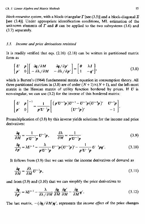
3.3. Income and price derivatives revisited
It is readily verified that eqs. (2.16)-(2.18) can be written in partitioned matrix form as
u P [ I[ %/dM
Pl 0 - ahlaM (3.8)
which is Barten’s (1964) fundamental matrix equation in consumption theory. All three partitioned matrices in (3.8) are of order (N + 1) x (N + l), and the left-most matrix is the Hessian matrix of utility function bordered by prices. If U is non-singular, we can use (3.2) for the inverse of this bordered matrix:
[I ;I-‘=*[ (p’u-‘p)u-‘-u-‘p(UFp)’ u-‘/J
(U_‘P)’ 1 -1 * Premultiplication of (3.8) by this inverse yields solutions for the income and price derivatives:
3L1u-~p, _?i=_L aM p’u-‘p aM pw- ‘p
_=Au-‘_ A % ap f
Pu-‘p(u-‘p)‘_ l pv- ‘p
pu-‘pqc p7- ‘p
(3.9)
(3.10)
It follows from (3.9) that we can write the income derivatives of demand as
&=-&u-Lp’ and from (3.9) and (3.10) that we can simplify the price derivatives to
i?L~U-‘- A __!ka4’_* 1
w aXlaM aM aM aMq *
(3.11)
(3.12)
The last matrix, - (*/aM)q’, represents the income effect of the price changes
16 H. Theil
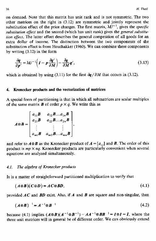
on demand. Note that this matrix has unit rank and is not symmetric. The two other matrices on the right in (3.12) are symmetric and jointly represent the substitution effect of the price changes. The first matrix, AU-‘, gives the specific substitution effect and the second (which has unit rank) gives the general substitu- tion effect. The latter effect describes the general competition of all goods for an extra dollar of income. The distinction between the two components of the substitution effect is from Houthakker (1960). We can combine these components by writing (3.12) in the form
(3.13)
which is obtained by using (3.11) for the first +/c?M that occurs in (3.12).
4. Kronecker products and the vectorization of matrices
A special form of partitioning is that in which all submatrices are scalar multiples of the same matrix B of order p x q. We write this as
a,,B a12B...alnB
a2,B azzB...a,,B A@B=. ..,
. . . . a,,B amaB...a,,B I
and refer to A@B as the Kronecker product of A = [aij] and B. The order of this product is mp x nq. Kronecker products are particularly convenient when several equations are analyzed simultaneously.
4.1. The algebra of Kronecker products
It is a matter of straightforward partitioned multiplication to verify that
(A@B)(C@D) = ACBBD, (4.1)
provided AC and BD exist. Also, if A and B are square and non-singular, then
(~633~’ = A-‘QDB-’ (4.2)
because (4.1) implies (A@B)(A-‘@B-l) = AA-‘@BB-’ = 181= I, where the three unit matrices will in general be of different order. We can obviously extend
Ch. I: Linear Algebra and Matrix Methoak 17
(4.1) to
provided A,A,A3 and B,B,B, exist. Other useful properties of Kronecker products are:
(A@B)‘= A’@B’, (4.3) A@(B+C)=A@B+A@C, (4.4) (B+C)sA=B@A+C%4, (4.5) A@(B@C) = (A@B)@C. (4.6)
Note the implication of (4.3) that A@B is symmetric when A and B are symmetric. Other properties of Kronecker products are considered in Section 7.
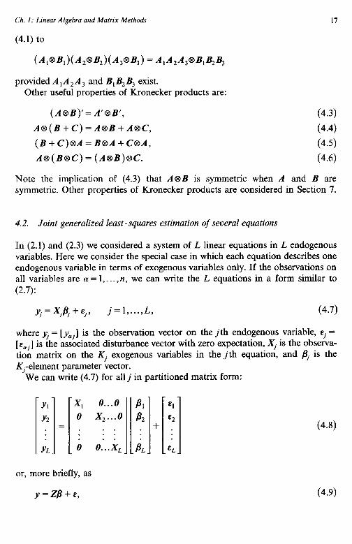
4.2. Joint generalized least-squares estimation of several equations
In (2.1) and (2.3) we considered a system of L linear equations in L endogenous variables. Here we consider the special case in which each equation describes one endogenous variable in terms of exogenous variables only. If the observations on all variables are (Y = 1 , . . . ,n, we can write the L equations in a form similar to (2.7):
*=X,lp,+e,, j=l ,“‘, L, (4.7)
where yj = [ yaj] is the observation vector on the j th endogenous variable, ej = [ eaj] is the associated disturbance vector with zero expectation, Xi is the observa- tion matrix on the Kj exogenous variables in the jth equation, and pj is the Kj-element parameter vector.
We can write (4.7) for all j in partitioned matrix form:
YI X, O...O 8, re,
Y2 0 X,...O /3, e2 = . . . + . . .
YL_ _ 0 0:. .X, S, ei
(4.8)
or, more briefly, as
y=@+e, (4.9)

18 H, Theil
where y and e are Ln-element vectors and Z contains Ln rows, while the number of columns of Z and that of the elements of B are both K, + . - . + K,. The covariance matrix of e is thus of order Ln X Ln and can be partitioned into L* submatrices of the form &(sjej). For j = 1 this submatrix equals the covariance matrix ‘V(sj). We assume that the n disturbances of each of the L equations have equal variance and are uncorrelated so that cV(.sj) = ~~1, where aij = vareaj (each a). For j z 1 the submatrix &(eje;) contains the “contemporaneous” covariances &(E,~E,,) for a=l,..., n in the diagonal. We assume that these covariances are all equal to uj, and that all non-contemporaneous covariances vanish: &(eaj.sll,) = 0 for (Y * n. Therefore, &(eje;) = uj,I, which contains V(E~) = uj, I as a special case. The full covariance matrix of the Ln-element vector e is thus:
u,J u,*I.. .u,,I
0211 u,,I...u*,I v4 = . . . = XSI, (4.10)
. . . .
_%,I u,,I...u,,I
where X = [?,I is the contemporaneous covariance matrix, i.e. the covariance matrix of [E u ,... E,~] for a=1 ,..., n.
Suppose that 2 is non-singular so that X- ’ 8 I is the inverse of the matrix (4.10) in view of (4.2). Also, suppose that X,, . . . , X, and hence Z have full column rank. Application of the GLS results (2.13) and (2.14) to (4.9) and (4.10) then yields
fi = [zyz-w)z]-‘Z’(X’c3I)y (4.11)
as the best linear unbiased estimator of /3 with the following covariance matrix:
V( )) = [z’(X-‘er)z] -‘. (4.12)
In general, b is superior to LS applied to each of the L equations separately, but there are two special cases in which these estimation procedures are identical.
The first case is that in which X,, . . . , X, are all identical. We can then write X for each of these matrices so that the observation matrix on the exogenous variables in (4.8) and (4.9) takes the form
x o...o 0 x...o
z=. . . I : =18X. . . .
0 0:-x
(4.13)

Ch. I: Linear Algebra and Matrix Methods
This implies
Z’(PCM)Z = (1@X)(z-‘@z)(z@x) =x-‘@XX
and
19
[z’(z-‘@z)z]-‘z’(x-‘~z) = [z@(x~x)-‘](zex~)(8-‘ez) =zo(x’x)-‘X’.
It is now readily verified from (4.11) that fi consists of L subvectors of the LS form (X’X)- ‘X’Y~. The situation of identical matrices X,, . . . ,X, occurs relatively frequently in applied econometrics; an example is the reduced form (2.4) for each of the L endogenous variables.
The second case in which (4.11) degenerates into subvectors equal to LS vectors is that of uncorrelated contemporaneous disturbances. Then X is diagonal and it is easily verified that B consists of subvectors of the form ( XiXj)- ‘Xj’y~. See Theil ( 197 1, pp. 3 1 l-3 12) for the case in which B is block-diagonal.
Note that the computation of the joint GLS estimator (4.11) requires B to be known. This is usually not true and the unknown X is then replaced by the sample moment matrix of the LS residuals [see Zellner (1962)]. This approxima- tion is asymptotically (for large n) acceptable under certain conditions; we shall come back to this matter in the opening paragraph of Section 9.
4.3. Vectorization of matrices
In eq. (2.3) we wrote Ln equations in matrix form with parameter matrices r and B, each consisting of several columns, whereas in (4.8) and (4.9) we wrote Ln equations in matrix form with a “long” parameter vector /3. If Z takes the form (4.13), we can write (4.8) in the equivalent form Y = XB + E, where Y, B, and E are matrices consisting of L columns of the form yi, sj, and ej. Thus, the elements of the parameter vector B are then rearranged into the matrix B. On the other hand, there are situations in which it is more attractive to work with vectors rather than matrices that consist of several columns. For example, if fi is an unbiased estimator of the parameter vector /3 with finite second moments, we obtain the covariance matrix of b by postmultiplying fi - /I by its transpose and taking the expectation, but this procedure does not work when the parameters are arranged in a matrix B which consists of several columns. It is then appropriate to rearrange the parameters in vector form. This is a matter of designing an appropriate notation and evaluating the associated algebra.
Let A = [a,... u4] be a p x q matrix, ai being the i th column of A. We define vecA = [a; a;... a:]‘, which is a pq-element column vector consisting of q
20 H. Theil
subvectors, the first containing the p elements of u,, the second the p elements of u2, and so on. It is readily verified that vec(A + B) = vecA +vecB, provided that A and B are of the same order. Also, if the matrix products AB and BC exist,
vecAB = (Z@A)vecB = (B’@Z)vecA,
vecABC= (Z@AB)vecC= (C’@A)vecB= (C’B’@Z)vecA.
For proofs and extensions of these results see Dhrymes (1978, ch. 4).
5. Differential demand and supply systems
The differential approach to microeconomic theory provides interesting compari- sons with equation systems such as (2.3) and (4.9). Let g(z) be a vector of functions of a vector z; the approach uses the total differential of g(o),
ag dg=-&z, (5.1)
and it exploits what is known about dg/&‘. For example, the total differential of consumer demand is dq = (Jq/aM)dM +( %/ap’)dp. Substitution from (3.13) yields:
dg=&(dM-p’dp)+hU’[dp-(+&d+], (5.4
which shows that the income effect of the price changes is used to deflate the change in money income and, similarly, the general substitution effect to deflate the specific effect. Our first objective is to write the system (5.2) in a more attractive form.
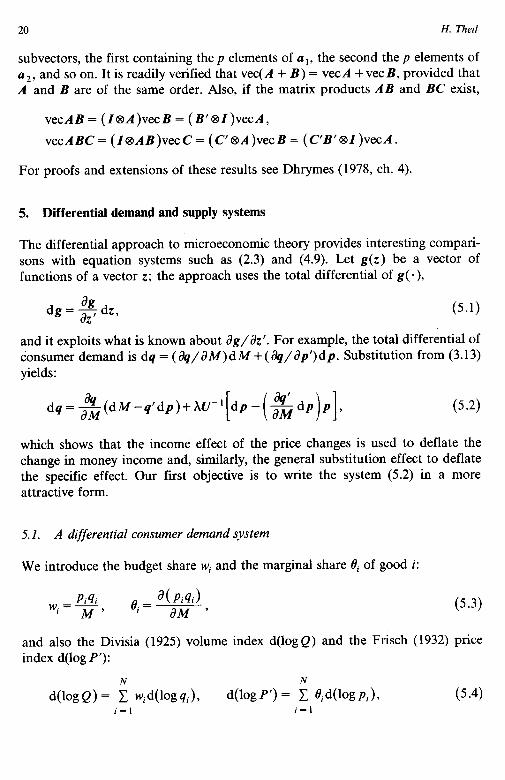
5.1. A differential consumer demand system
We introduce the budget share wj and the marginal share ei of good i:
Pi4i wi=-, M 8, = a( Pi4i)
1 ad49 (5.3)
and also the Divisia (1925) volume index d(log Q) and the Frisch (1932) price index d(log P’):
d(logQ) = !E wid(logqi)> d(logP’) = ; Bid(logpi), (5.4) i=l i=l
Ch. I: Linear Algebra and Matrix Methods 21
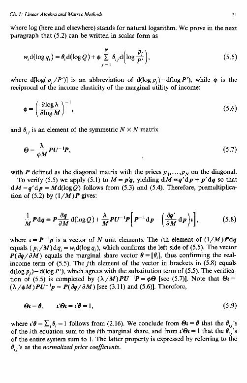
where log (here and elsewhere) stands for natural logarithm. We prove in the next paragraph that (5.2) can be written in scalar form as
N
wid(logqi)=Bid(logQ)+$ C Oiid 65) j=l
where d[log( p,/P’)] is an abbreviation of d(logpj)-d(log P'), while $I is the reciprocal of the income elasticity of the marginal utility of income:
dlogX -’ += a1ogA4 ’ i 1
and eii is an element of the symmetric N X N matrix
8 = &,u- ‘P,
(5.6)
(5 -7)
with P defined as the diagonal matrix with the prices p,, . . . ,pN on the diagonal. To verify (5.5) we apply (5.1) to M = p?~, yielding dM =q’dp + p’dq so that
dM -q’dp = Md(log Q) follows from (5.3) and (5.4). Therefore, premultiplica- tion of (5.2) by (l/M)P gives:
84 $Pdq=PaMd(logQ)+$PU-‘P t5m8)
where 1= P- 'p is a vector of N unit elements. The ith element of (l/M)Pdq equals ( pi/M)dqi = w,d(log qi), which confirms the left side of (5.5). The vector P( dq/JM) equals the marginal share vector ~9 = [Oil, thus confirming the real- income term of (5.5). The jth element of the vector in brackets in (5.8) equals d(log pj)- d(log P'), which agrees with the substitution term of (5.5). The verifica- tion of (5.5) is completed by (X/M)PU-‘P= $43 [see (5.7)]. Note that 8&= (X/cpM)PU-‘p = P( +/JM) [see (3.11) and (5.6)]. Therefore,
6h=e, dec = de = I, 6%
where 1’8 = xi 0, = 1 follows from (2.16). We conclude from &= 0 that the eij’s of the ith equation sum to the ith marginal share, and from L’& = 1 that the fIij’s of the entire system sum to 1. The latter property is expressed by referring to the eij’s as the normalized price coefficients.

22 H. Theil
5.2. A comparison with simultaneous equation systems
The N-equation system (5.5) describes the change in the demand for each good, measured by its contribution to the Divisia index [see (5.4)],2 as the sum of a real-income component and a substitution component. This system may be compared with the L-equation system (2.1). There is a difference in that the latter system contains in principle more than one endogenous variable in each equation, whereas (5.5) has only one such variable if we assume the d(logQ) and all price changes are exogenous.3 Yet, the differential demand system is truly a system because of the cross-equation constraints implied by the symmetry of the normal- ized price coefficient matrix 8.
A more important difference results from the utility-maximizing theory behind (5.5), which implies that the coefficients are more directly interpretable than the y’s and p’s of (2.1). Writing [e”] = 8-l and inverting (5.7), we obtain:
eij- cpM a2u A a( Pi4i) ‘( Pjqj) ’
(5.10)
which shows that B’j measures (apart from +M/h which does not involve i andj) the change in the marginal utility of a dollar spent on i caused by an extra dollar spent on j. Equivalently, the normalized price coefficient matrix 8 is inversely proportional to the Hessian matrix of the utility function in expenditure terms.
The relation (5.7) between 8 and U allows us to analyze special preference structures. Suppose that the consumer’s tastes can be represented by a utility function which is the sum of N functions, one for each good. Then the marginal utility of each good is independent of the consumption of all other goods, which we express by referring to this case as preference independence. The Hessian U is then diagonal and so is 8 [see (5.7)], while @I= 6 in (5.9) is simplified to Oii = 0,. Thus, we can write (5.5) under preference independence as
wid(logqi) = e,d(logQ)+&d(log$), (5.11)
which contains only one Frisch-deflated price. The system (5.11) for i = 1,. . . ,N contains only N unconstrained coefficients, namely (p and N - 1 unconstrained marginal shares.
The apphcation of differential demand systems to data requires a parameteriza- tion which postulates that certain coefficients are constant. Several solutions have
‘Note that this way of measuring the change in demand permits the exploitation of the symmetry of 8. When we have d(log qi) on the left, the coefficient of the Frisch-deflated price becomes 8ij/w,, which is an element of an asymmetric matrix.
3This assumption may be relaxed; see Theil(1975-76, ch. 9- 10) for an analysis of endogenous price changes.
Ch. 1: Linear Algebra and Matrix Methods 23
been proposed, but these are beyond the scope of this chapter; see the references quoted in Section 2.4 above and also, for a further comparison with models of the type (2.1), Theil and Clements (1980).
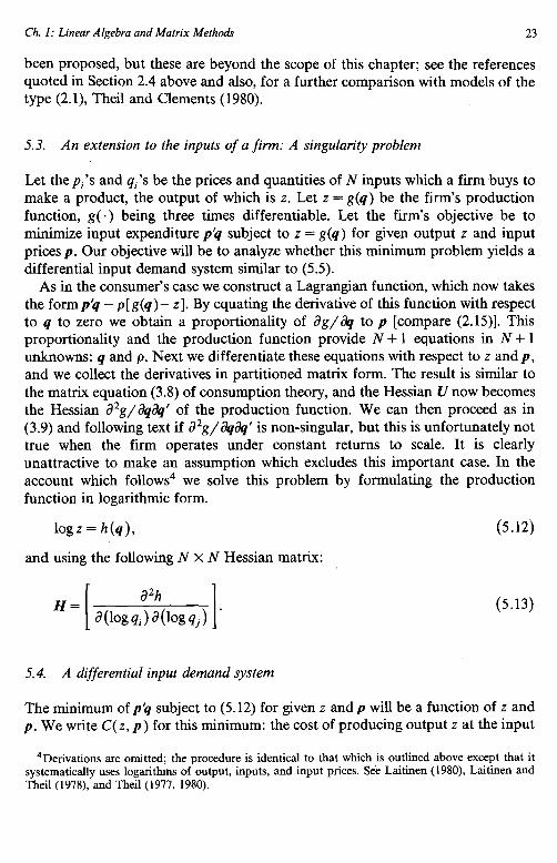
5.3. An extension to the inputs of a firm: A singularity problem
Let the pi's and qi’s be the prices and quantities of N inputs which a firm buys to make a product, the output of which is z. Let z = g(q) be the firm’s production function, g( .) being three times differentiable. Let the firm’s objective be to minimize input expenditure p’q subject to z = g(q) for given output z and input prices p. Our objective will be to analyze whether this minimum problem yields a differential input demand system similar to (5.5).
As in the consumer’s case we construct a Lagrangian function, which now takes the form p’q - p[ g(q) - z]. By equating the derivative of this function with respect to q to zero we obtain a proportionality of ag/&I to p [compare (2.15)]. This proportionality and the production function provide N + 1 equations in N + 1 unknowns: q and p. Next we differentiate these equations with respect to z and p, and we collect the derivatives in partitioned matrix form. The result is similar to the matrix equation (3.8) of consumption theory, and the Hessian U now becomes the Hessian a2g/&&’ of the production function. We can then proceed as in (3.9) and following text if a2g/Jqa’ is non-singular, but this is unfortunately not true when the firm operates under constant returns to scale. It is clearly unattractive to make an assumption which excludes this important case. In the account which follows4 we solve this problem by formulating the production function in logarithmic form.
and
logz = h(q), using the following N X N Hessian matrix:
H= a*h
1 W%qi)W%qj) .
(5.13)
5.4. A differential input demand system
The minimum of p’q subject to (5.12) for given z and p will be a function of z and _
(5.12)
p. We write C(z, p) for this minimum: the cost of producing output z at the input
4Derivations are omitted; the procedure is identical to that which is outlined above except that it systematically uses logarithms of output, inputs, and input prices. See Laitinen (1980), Laitinen and Theil(1978), and Theil (1977, 1980).

24 H. Theil
prices p. We define
a1ogc ill,1 PlogC y=alogz’ $ Y2 a(logz)” ’
(5.14)
so that y is the output elasticity of cost and J, < 1 ( > 1) when this elasticity increases (decreases) with increasing output; thus, 1c/ is a curvature measure of the logarithmic cost function. It can be shown that the input demand equations may be written as
fid(logqi) =yt$d(logz)-rC, ; B,jd(log$), j=l
(5.15)
which should be compared with (5.5). In (5.15),fi is the factor share of input i (its share in total cost) and 0, is its marginal share (the share in marginal cost),
(5.16)
which is the input version of (5.3). The Frisch price index on the far right in (5.15) is as shown in (5.4) but with fii defined in (5.16). The coefficient Oij in (5.15) is the (i, j)th element of the symmetric matrix
8 = iF(F- yH)-‘F, (5.17)
where H is given in (5.13) and F is the diagonal matrix with the factor shares f,, . . . ,fN on the diagonal. This 8 satisfies (5.9) with 8 = [t9,] defined in (5.16).
A firm is called input independent when the elasticity of its output with respect to each input is independent of all other inputs. It follows from (5.12) and (5.13) that H is then diagonal; hence, 8 is also diagonal [see (5.17)] and 8&= 0 becomes Oii = 8, so that we can simplify (5.15) to
f,d(logq,)=yB,d(logz)-#8,d(log$+ (5.18)
which is to be compared with the consumer’s equation (5.11) under preference independence. The Cobb-Douglas technology is a special case of input indepen- dence with H = 0, implying that F( F - yH)- ‘F in (5.17) equals the diagonal matrix F. Since Cobb-Douglas may have constant returns to scale, this illustrates that the logarithmic formulation successfully avoids the singularity problem mentioned in the previous subsection.

Ch. 1: Linear Algebra and Matrix Methods 25
5.5. Allocation systems
Summation of (5.5) over i yields the identity d(logQ) = d(log Q), which means that (5.5) is an allocation system in the sense that it describes how the change in total expenditure is allocated to the N goods, given the changes in real income and relative prices. To verify this identity, we write (5.5) for i = 1,. . . ,N in matrix form as
WK = (l’WK)8 + @(I - LB’)Q, (5.19)
where W is the diagonal matrix with w,, . . . , wN on the diagonal and A = [d(log pi)] and K = [d(log qi)] are the vectors logarithmic price and quantity changes so that d(logQ) = L’WK, d(log P’) = B’s. The proof is completed by premultiplying (5.19) by L’, which yields ~WK = ~WK in view of (5.9). Note that the substitution terms of the N demand equations have zero sum.
The input demand system (5.15) is not an allocation system because the firm does not take total input expenditure as given; rather, it minimizes this expendi- ture for given output z and given input prices p. Summation of (5.15) over i yields:
d(logQ) = ud(lw), (5.20)
where d(log Q) = xi fid(log qi) = L’FK is the Divisia input volume index. Substitu- tion of (5.20) into (5.15) yields:
fid(logqi)=Bid(logQ)-4 ; tiijd(log+). j = 1
(5.21)
We can interpret (5.20) as specifying the aggregate input change which is required to produce the given change in output, and (5.21) as an allocation system for the individual inputs given the aggregate input change and the changes in the relative input prices. It follows from (5.9) that we can write (5.19) and (5.21) for each i as
wK= (I’wK)eL+cpe(I--ll’e)Q, (5.22)
FK= (C’1oK)8L--\cle(I-LL’e)n, (5.23)
which shows that the normalized price coefficient matrix 8 and the scalars C#I and # are the only coefficients in the two allocation systems.
5.6. Extensions
Let the firm adjust output z by maximizing its profit under competitive condi- tions, the price y of the product being exogenous from the firm’s point of view.
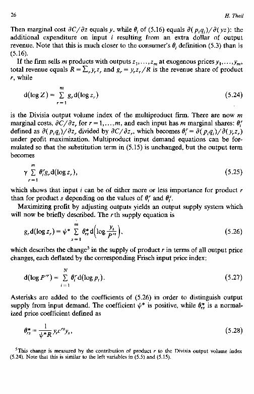
26 H. Theil
Then marginal cost aC/az equals y, while Oi of (5.16) equals a( piqi)/a( yz): the additional expenditure on input i resulting from an extra dollar of output revenue. Note that this is much closer to the consumer’s Si definition (5.3) than is (5.16).
If the firm sells m products with outputs z,, . . . , z, at exogenous prices y,, . . . ,y,, total revenue equals R = &yrz, and g, = y,z,/R is the revenue share of product r, while
d(loiG) = ;1: g,d(lw,) (5.24) r=l
is the Divisia output volume index of the multiproduct firm. There are now m marginal costs, ac/aZ, for r = 1,. . . , m, and each input has m marginal shares: 9; defined as a( piqi)/azr divided by X/az,, which becomes 0; = a( piqi)/a( y,z,) under profit maxitiation. Multiproduct input demand equations can be for- mulated so that the substitution term in (5.15) is unchanged, but the output term becomes
(5.25)
which shows that input i can be of either more or less importance for product r than for product s depending on the values of 13: and 13,“.
Maximizing profit by adjusting outputs yields an output supply system which will now be briefly described. The r th supply equation is
grd&w,) = ~*s~,W(log$s)~ (5.26)
which describes the change’ in the supply of product r in terms of all output price changes, each deflated by the corresponding Frisch input price index:
d(log P”) = ; B,‘d(logp;). i=l
(5.27)
Asterisks are added to the coefficients of (5.26) in order to distinguish output supply from input demand. The coefficient $* is positive, while 0: is a normal- ized price coefficient defined as
(5.28)
‘This change is measured by the contribution of product r to the Divisia output volume index (5.24). Note that this is similar to the left variables in (5.5) and (5.15).

Ch. I: Linear Algebra and Matrix Methods 27
where crs is an element of the inverse of the symmetric m x m matrix [ a*C/az, az,]. The similarity between (5.28) and (5.7) should be noted; we shall consider this matter further in Section 6. A multiproduct firm is called output independent when its cost function is the sum of m functions, one for each product.6 Then [ d*C/az, az,] and [Q] are diagonal [see (5.28)] so that the change in the supply of each product depends only on the change in its own deflated price [see (5.26)]. Note the similarity to preference and input independence [see (5.11) and (5.18)].
6. Definite and semidefinite square matrices
The expression x’Ax is a quadratic form in the vector X. We met several examples in earlier sections: the second-order term in the Taylor expansion (2.6), E’ME in the residual sum of squares (2.12), the expression in the exponent in the normal density function (3.3), the denominator p'U_ 'p in (3.9), and &3~ in (5.9). A more systematic analysis of quadratic forms is in order.
6.1. &variance matrices and Gauss -Markov further considered
Let r be a random vector with expectation Gr and covariance matrix 8. Let w’r be a linear function of r with non-stochastic weight vector w so that &( w’r) = w’&r.
The variance of w’r is the expectation of
[w’(r-&r)]*=w’(r-&r)(r-&r)‘w,
so that var w’r = w’v(r)w = w%w. Thus, the variance of any linear function of r
equals a quadratic form with the covariance matrix of r as matrix. If the quadratic form X’AX is positive for any x * 0, A is said to be positive
definite. An example is a diagonal matrix A with positive diagonal elements. If x’Ax > 0 for any x, A is called positive semidefinite. The covtiance matrix X of any random vector is always positive semidefinite because we just proved that w%w is the variance of a linear function and variances are non-negative. This covariance matrix is positive semidefinite but not positive definite if w%w = 0 holds for some w * 0, i.e. if there exists a non-stochastic linear function of the random vector. For example, consider the input allocation system (5.23) with a
6Hall (1973) has shown that the additivity of the cost function in the m outputs is a necessary and sufficient condition in order that the multiproduct firm can be broken up into m single-product firms in the following way: when the latter firms independently maximize profit by adjusting output, they use the same aggregate level of each input and produce the same level of output as the multiproduct firm.
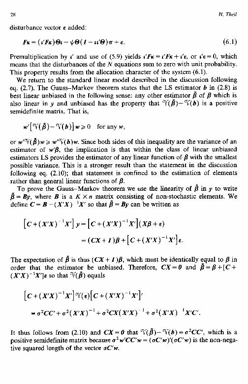
28 H. Theil
disturbance vector e added:
Premultiplication by 1’ and use of (5.9) yields L’FK = L’FK + de, or 1’~ = 0, which means that the disturbances of the N equations sum to zero with unit probability. This property results from the allocation character of the system (6.1).
We return to the standard linear model described in the discussion following eq. (2.7). The Gauss-Markov theorem states that the LS estimator b in (2.8) is best linear unbiased in the following sense: any other estimator B of j3 which is also linear in y and unbiased has the property that V(b)- V(b) is a positive semidefinite matrix. That is,
w’[V(j)-Y(b)]w>O foranyw,
or w’?r( /?)w > w’V(b)w. Since both sides of this inequality are the variance of an estimator of w’& the implication is that within the class of linear unbiased estimators LS provides the estimator of any linear function of /3 with the smallest possible variance. This is a stronger result than the statement in the discussion following eq. (2.10); that statement is confined to the estimation of elements rather than general linear functions of &
To prove the Gauss-Markov theorem we use the linearity of fl in y to write B = By, where B is a K x n matrix consisting of non-stochastic elements. We define C = B - (XX)- ‘X’ so that fi = By can be written as
[c+(rx)-‘xj y= [c+(rx)_‘X’](x#l+e)
=(cx+z)/3+[c+(X~x)-‘X’]E.
The expectation of B is thus (CX + Z)/3, which must be identically equal to /3 in order that the estimator be unbiased. Therefore, CX = 0 and B = /3 + [C + (X’X))‘X’]e so that V(B) equals
[c+(rx)-‘X’]qe)[C+(X’X)-‘X’]’
=&CC’+ a*(X’X)-‘+ u*CX(X’X)-‘+ u*(X’X)-‘XC
It thus follows from (2.10) and CX=O that V(b)-V(b)= a*CC’, which is a positive semidefinite matrix because a* w’CC’W = (aC’w)‘( aC’w) is the non-nega- tive squared length of the vector uC’W.

Ch. I: Linear Algebra and Matrix Methods 29
6.2. Maxima and minima
The matrix A is called negative semidefinite if X’AX < 0 holds for any x and negative definite if X’AX < 0 holds for any x * 0. If A is positive definite, - A is negative definite (similarly for semidefiniteness). If A is positive (negative) definite, all diagonal elements of A are positive (negative). This may be verified by considering x’Ax with x specified as a column of the unit matrix of ap- propriate order. If A is positive (negative) definite, A is non-singular because singularity would imply the existence of an x f 0 so that Ax = 0, which is contradicted by X’AX > 0 ( -c 0). If A is symmetric positive (negative) definite, so is A-‘, which is verified by considering x’Ax with x = A - ‘y for y * 0.
For the function g( *) of (2.6) to have a stationary value at z = z it is necessary and sufficient that the gradient ag/& at this point be zero. For this stationary value to be a local maximum (minimum) it is sufficient that the Hessian matrix a’g/az& at this point be negative (positive) definite. We can apply this to the supply equation (5.26) which is obtained by adjusting the output vector z so as to maximize profit. We write profit as y’z - C, where y is the output price vector and C = cost. The gradient of profit as a function of z is y - aC/az ( y is indepen- dent of z because y is exogenous by assumption) and the Hessian matrix is - a2C/&&’ so that a positive definite matrix a2C/azaz’ is a sufficient condi- tion for maximum profit. Since #* and R in (5.28) are positive, the matrix [@A] of the supply system (5.26) is positive definite. The diagonal elements of this matrix are therefore positive so that an increase in the price of a product raises its supply.
Similarly, a sufficient conditions for maximum utility is that the Hessian U be negative definite, implying cp < 0 [see (3.9) and (5.6)], and a sufficient condition for minimum cost is that F - -yH in (5.17) be positive definite. The result is that [Oi,] in both (5.5) and (5.15) is also positive definite. Since (p and - $ in these equations are negative, an increase in the Frisch-deflated price of any good (consumer good or input) reduces the demand for this good. For two goods, i and j, a positive (negative) ~9~~ = eii implies than an increase in the Frisch-deflated price of either good reduces (raises) the demand for the other; the two goods are then said to be specific complements (substitutes). Under preference or input independence no good is a specific substitute or complement of any other good [see (5.11) and (5.18)]. The distinction between specific substitutes and comple- ments is from Houthakker (1960); he proposed it for consumer goods, but it can be equally applied to a firm’s inputs and also to outputs based on the sign of 02 = 6’: in (5.26).
The assumption of a definite U or F - yH is more than strictly necessary. In the consumer’s case, when utility is maximized subject to the budget constraint p’q = M, it is sufficient to assume constrained negative definiteness, i.e. x’Ux < 0 for all x * 0 which satisfy p'x = 0. It is easy to construct examples of an indefinite

30 H. Theil
or singular semidefinite matrix U which satisfy this condition. Definiteness obviously implies constrained definiteness; we shall assume that U and 1: - yH satisfy the stronger conditions so that the above analysis holds true.
6.3. Block -diagonal definite matrices
If a matrix is both definite and block-diagonal, the relevant principal submatrices are also definite. For example, if X of (3.4) is positive definite, then .+X,x, + x;Z,x, > 0 if either x, f 0 or xZ f 0, which would be violated if either X, or E2 were not definite.
Another example is that of a logarithmic production function (5.12) when the inputs can be grouped into input groups so that the elasticity of output with respect to each input is independent of all inputs belonging to different groups. Then H of (5.13) is block-diagonal and so is 8 [see (5.17)]. Thus, if i belongs to input group Sg (g = 1,2,. . .), the summation over j in the substitution term of (5.15) can be confined toj E Sp; equivalently, no input is then a specific substitute or complement of any input belonging to a different group. Also, summation of the input demand equations over all inputs of a group yields a composite demand equation for the input group which takes a similar form, while an appropriate combination of this composite equation with a demand equation for an individual input yields a conditional demand equation for the input within their group. These developments can also be applied to outputs and consumer goods, but they are beyond the scope of this chapter.
7. Diagonalizations
7.1. The standard diagonalization of a square matrix
For some n X n matrix A we seek a vector x so that Ax equals a scalar multiple A of x. This is trivially satisfied by x = 0, so we impose x’x = 1 implying x * 0. Since Ax = Xx is equivalent to (A - X1)x = 0, we thus have
(A-hl)x=O, x)x=1, (7.1)
so that A - XI is singular. This implies a zero determinant value,
IA - AI\ = 0, (7.2)
which is known as the characteristic equation of A. For example, if A is diagonal
Ch. I: Linear Algebra and Matrix Metho& 31
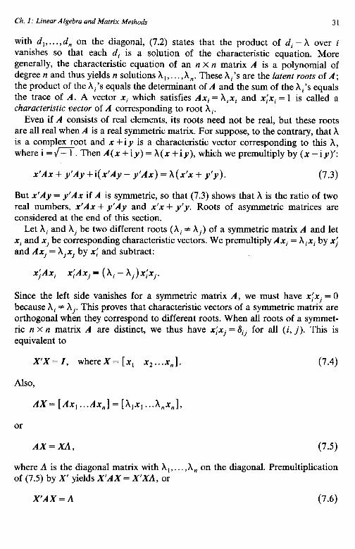
with d ,, . . . ,d, on the diagonal, (7.2) states that the product of di - A over i vanishes so that each di is a solution of the characteristic equation. More generally, the characteristic equation of an n x n matrix A is a polynomial of degree n and thus yields n solutions X, , . . . , A,,. These Ai’s are the latent roots of A; the product of the Ai’s equals the determinant of A and the sum of the Xi’s equals the trace of A. A vector xi which satisfies Axi = hixi and x;xi = 1 is called a characteristic vector of A corresponding to root Xi.
Even if A consists of real elements, its roots need not be real, but these roots are all real when A is a real symmetric matrix. For suppose, to the contrary, that h is a complex root and x + iy is a characteristic vector corresponding to this X, wherei=m.ThenA(x+iy)=h(x+iy), whichwepremultiplyby(x-iy)‘:
x’Ax + y’Ay + i( x’Ay - y/Ax) = X (x’x + y’y ) . (7.3)
But x’Ay = y’Ax if A is symmetric, so that (7.3) shows that X is the ratio of two real numbers, x’Ax + y’Ay and x’x + y’y. Roots of asymmetric matrices are considered at the end of this section.
Let Xi and Xj be two different roots (hi * Xj) of a symmetric matrix A and let xi and xj be corresponding characteristic vectors. We premultiply Ax, = Xixi by xJI and Axj = Xjxj by xi and subtract:
xj’Axi - x;Axj = (Xi - Xj)x;xj.
Since the left side vanishes for a symmetric matrix A, we must have x;xj = 0 because Xi * Aj. This proves that characteristic vectors of a symmetric matrix are orthogonal when they correspond to different roots. When all roots of a symmet- ric n x n matrix A are distinct, we thus have xixj = aij for all (i, j). This is equivalent to
X’X=I, whereX= [x, +...x,]. (7.4)
Also.
AX= [Ax, . ..Ax.] = [X,x, . ..X”x.],
or
AX= XA, (7.5)
where A is the diagonal matrix with h,, . . . , A, on the diagonal. Premultiphcation of (7.5) by X’ yields X’AX = X’XA, or
X’AX = A (7.6)
32 H. Theil
in view of (7.4). Therefore, when we postmultiply a symmetric matrix A by a matrix X consisting of characteristic vectors of A and premultiply by X’, we obtain the diagonal matrix containing the latent roots of A. This double multipli- cation amounts to a diagonalization of A. Also, postmultiplication of (7.5) by X’ yields AXX’ = XAX’ and hence, since (7.4) implies X’ = X-’ or XX’ = 1,
A = XAX’= i &x,x;. (7.7) i=l
In the previous paragraph we assumed that the Ai’s are distinct, but it may be shown that for any symmetric A there exists an X which satisfies (7.4)-(7.7), the columns of X being characteristic vectors of A and A being diagonal with the latent roots of A on the diagonal. The only difference is that in the case of multiple roots (Ai = Aj for i * j) the associated characteristic vectors (xi and fj) are not unique. Note that even when all X’s are distinct, each xi may be arbitrarily multiplied by - 1 because this affects neither Axi = hixi nor xjxj = 0 for any (i, j); however, this sign indeterminacy will be irrelevant for our purposes.
7.2. Special cases
Let A be square and premultiply Ax = Xx by A to obtain A2x = XAx = X2x. This shows that A2 has the same characteristic vectors as A and latent roots equal to the squares of those of A. In particular, if a matrix is symmetric idempotent, such as M of (2.1 l), all latent roots are 0 or 1 because these are the only real numbers that do not change when squared. For a symmetric non-singular A, p&multiply Ax = Ax by (AA)-’ to obtain A-lx= (l/A)x. Thus, A-’ has the same character- istic vectors as those of A and latent roots equal to the reciprocals of those of A. If the symmetric n x n matrix A is singular and has rank r, (7.2) is satisfied by X = 0 and this zero root has multiplicity n - r. It thus follows from (7.7) that A can then be written as the sum of r matrices of unit rank, each of the form hixixi, with Ai * 0.
Premultiplication of (7.7) by Y’ and postmultiplication by y yields y’Ay = ciXic,?, with ci = y’xi. Since y’Ay is positive (negative) for any y f 0 if A is positive (negative) definite, this shows that all latent roots of a symmetric positive (negative) definite matrix are positive (negative). Similarly, all latent roots of a symmetric positive (negative) semidefinite matrix are non-negative (non-positive).
Let A,,, be a symmetric m x m matrix with roots A,, . . . ,A, and characteristic vectors x,,...,x,; let B,, be a symmetric n x n matrix with roots p,, . . . ,p,, and characteristic vectors y,, . . . , y,,. Hence, A,,,@Bn is of order mn X mn and has mn latent roots and characteristic vectors. We use Amxi = Xixi and B,, yj = pjyj in
(A,eB~)(Xi~Yj)=(A,xi)‘(B,~)=(‘ixi)’(~jYj)=’i~j(Xi’vi),
Oz. 1: Linear Algebra and Matrix h4erhoh 33
which shows that xi@y, is a characteristic vector of A,@B, corresponding to root A,pj. It is easily venf’ed that these characteristic vectors form an orthogonal matrix of order mn x mn:
Since the determinant of A,@B, equals the product of the roots, we have
It may similarly be verified that the rank (trace) of A,@B, equals the product of the ranks (traces) of A,,, and B,.
7.3. Aitken’s theorem
Any symmetric positive definite matrix A can be written as A = QQ’, where Q is some non-singular matrix. For example, we can use (7.7) and specify Q = XA1i2, where AlI2 is the diagonal matrix which contains the positive square roots of the latent roots of A on the diagonal. Since the roots of A are all positive, AlI2 is non-singular; X is non-singular in view of (7.4); therefore, Q = XA’12 is also non-singular.
Consider in particular the disturbance covariance matrix a2V in the discussion preceding eq. (2.13). Since u2 > 0 and V is non-singular by assumption, this covariance matrix is symmetric positive definite. Therefore, V- ’ is also symmetric positive definite and we can write V- ’ = QQ’ for some non-singular Q. We premultiply (2.7) by Q’:
Q’y = (Q’X)/3 + Q’E. (7.8)
The disturbance vector Q’e has zero expectation and a covariance matrix equal to
cr2Q’VQ=a2Q’(QQ’)-‘Q=cr2Q’(Q’)-‘Q-’Q=u21,
so that the standard linear model and the Gauss-Markov theorem are now applicable. Thus, we estimate j3 by applying LS to (7.8):
which is the GLS estimator (2.13). The covariance matrix (2.14) is also easily verified.

34 H. Theil
7.4. The Cholesky decomposition
The diagonalization (7.6) uses an orthogonal matrix X [see (7.4)], but it is also possible to use a triangular matrix. For example, consider a diagonal matrix D and an upper triangular matrix C with units in the diagonal,
c= 0 I 0
yielding
C’DC = d, d,c,* d,c,,
d,c,2 d,c;z + d2 dlW13 + d2c23 -
dlC13 d,c,,c,, + 4c2, d,c& + d,c;, + d, 1 It is readily verified that any 3 x 3 symmetric positive definite matrix A = [aij] can be uniquely written as C’DC (d, = a, ,, c,~ = ~,~/a,,, etc.). This is the so-called Cholesky decomposition of a matrix; for applications to demand analysis see Barten and Geyskens (1975) and Theil and Laitinen (1979). Also, note that D = (C’)- ‘AC- ’ and that C- ’ is upper triangular with units in the diagonal.
7.5. Vectors written as diagonal matrices
On many occasions we want to write a vector in the form of a diagonal matrix. An example is the price vector p which occurs as a diagonal matrix P in (5.8). An alternative notation is @, with the hat indicating that the vector has become a diagonal matrix. However, such notations are awkward when the vector which we want to write as a diagonal matrix is itself the product of one or several matrices and a vector. For example, in Section 8 we shall meet a nonsingular N X N matrix X and the vector X- ‘6. We write this vector in diagonal matrix form as
0
CjX2j
0
. . .
. . .
. . .
where xij is an element of X- ’ and all summations are overj = 1,. . . , N. It is easily
Ch. I: Linear Algebra and Matrix MethodF
verified that
(X-‘&l = X-‘6, 6yx-‘6), = Iyxy’.
35
(7.10)
7.6. A simultaneous diagonalization of two square matrices
We extend (7.1) to
(A-XB)x=U, x’Bx=l, (7.11)
where A and B are symmetric n X n matrices, B being positive definite. Thus, B- ’ is symmetric positive definite so that B- ’ = QQ’ for some non-singular Q. It is easily seen that (7.11) is equivalent to
(Q’AQ-XI)~=O, fy=i, Y=~-k (7.12)
This shows that (7.11) can be reduced to (7.1) with A interpreted as Q’AQ. If A is symmetric, so is Q’AQ. Therefore, all results for symmetric matrices described earlier in this section are applicable. In particular, (7.11) has n solutions, A,, . . . ,A, and n ,,..., x,, the xi’s being unique when the hi’s are distinct. From y,‘yj = Sij and yi = Q- ‘xi we have xjBxj = tiij and hence X’BX = I, where X is the n x n matrix with xi as the ith column. We write (A - XB)x = 0 as Axi = hiBxi for the ith solution and as AX = BXA for all solutions jointly, where A is diagonal with x ,, . . . ,A, on the diagonal. Premultiplication of AX = BXA by X’ then yields X’AX = X’BXA = A. Therefore,
X’AX=A, X’BX = I, (7.13)
which shows that both matrices are simultaneously diagonalized, A being trans- formed into the latent root matrix A, and B into the unit matrix.
It is noteworthy that (7.11) can be interpreted in terms of a constrained extremum problem. Let us seek the maximum of the quadratic form X’AX for variations in x subject to X’BX = 1. So we construct the Lagrangian function x’Ax - p( X’BX - l), which we differentiate with respect to x, yielding 2Ax - 2pBx. By equating this derivative to zero we obtain Ax = pBx, which shows that p must be a root hi of (7.11). Next, we premultiply Ax = pBx by x’, which gives x’Ax = px’Bx = p and shows that the largest root Ai is the maximum of x’Ax subject to X’BX = 1. Similarly, the smallest root is the minimum of x’Ax subject to X’BX = 1, and all n roots are stationary values of x’Ax subject to X’BX = 1.

36 H. Theil
7.7. Latent roots of an asymmetric matrix
Some or all latent roots of an asymmetric square matrix A may be complex. If (7.2) yields complex roots, they occur in conjugate complex pairs of the form a f bi. The absolute value of such a root is defined as dm, which equals [al if b = 0, i.e. if the root is real. If A is asymmetric, the latent roots of A and A’ are still the same but a characteristic vector of A need not be a characteristic vector of A’. If A is asymmetric and has multiple roots, it may have fewer characteristic vectors than the number of its rows and columns. For example,
is an asymmetric 2x2 matrix with a double unit root, but it has only one characteristic vector, [ 1 01’. A further analysis of this subject involves the Jordan canonical form, which is beyond the scope of this chapter; see Bellman (1960, ch. 11).
Latent roots of asymmetric matrices play a role in the stability analysis of dynamic equations systems. Consider the reduced form
y, = 4 + Ay,_, + x4*x, + u,, (7.14)
where s: is an L-element observation vector on endogenous variables at time t, a is a vector of constant terms, A is a square coefficient matrix, A* is an L X K coefficient matrix, x, is a K-element observation vector on exogenous variables at t, and U, is a disturbance vector. Although A is square, there is no reason why it should be symmetric so that its latent roots may include conjugate complex pairs. In the next paragraph we shall be interested in the limit of A” as s + co. Recall that A2 has roots equal to the squares of those of A ; this also holds for the complex roots of an asymmetric A. Therefore, A” has latent roots equal to the s th power of those of A. If the roots of A are all less than 1 in absolute value, those of AS will all converge to zero as s + co, which means that the limit of A” for s + co is a zero matrix. Also, let S = I + A + * . - + AS; then, by subtracting AS = A + A*+ . . . +A”+’ we obtain (I - A)S = I - AS+’ so that we have the following result for the limit of S when all roots of A are less than 1 in absolute value:
lim (I+A+ **. +X)=(1-A)_‘. (7.15) s-r00
We proceed to apply these results to (7.14) by lagging it by one period, Ye_ I = (I + Ay,_, + A*x,_, + ul_ I, and substituting this into (7.14):
y,=(I+A)a+A* Js_* + A*x, + kU*x,_, + u, + Au,_,

Ch. I: Linear Algebra and Matrix Methodr 31
When we do this s times, we obtain:
y,=(I+A+ ... + A”)a + AS+‘y,_s_,
+ A*x, + AA*+, + . . . + A”A*x,_,
+ u, + Au,_, + . . . + AS~t_s. (7.16)
If all roots of A are less than 1 in absolute value, so that A” converges to zero as s -+ cc and (7.15) holds, the limit of (7.16) for s + co becomes
y,=(I-A)-‘a+ E ASA*x,_s+ E Ah_,, (7.17) s=o s=o
which is the final form of the equation system. This form expresses each current endogenous variable in terms of current and lagged exogenous variables as well as current and lagged disturbances; all lagged endogenous variables are eliminated from the reduced form (7.14) by successive lagged application of (7.14). The coefficient matrices A”A* of xl_, for s = 0,1,2, . . . in (7.17) may be viewed as matrix multipliers; see Goldberger (1959). The behavior of the elements of ASA* as s + cc is dominated by the root of A with the largest absolute value. If this root is a conjugate complex pair, the behavior of these elements for increasing s is of the damped oscillatory type.
Endogenous variables occur in (7.14) only with a one-period lag. Suppose that Ay,_, in (7.14) is extended to A, y,_, + - - - + A,y,_,, where r is the largest lag which occurs in the equation system. It may be shown that the relevant de- terminantal equation is now
1X(-1)+X’-‘A,+ -.. +A,I=O. (7.18)
When there are L endogenous variables, (7.18) yields LT solutions which may include conjugate complex pairs. All these solutions should be less than 1 in absolute value in order that the system be stable, i.e. in order that the coefficient matrix of x,_~ in the final form converges to zero as s + co. It is readily verified that for 7 = 1 this condition refers to the latent roots of A,, in agreement with the condition underlying (7.17).
8. Principal components and extensions
8.1. Principal components
Consider an n X K observation matrix 2 on K variables. Our objective is to approximate Z by a matrix of unit rank, ue’, where u is an n-element vector of
38 H. Theil
values taken by some variable (to be constructed below) and c is a K-element coefficient vector. Thus, the approximation describes each column of Z as proportional to v. It is obvious that if the rank of Z exceeds 1, there will be a non-zero n x K discrepancy matrix Z - vc’ no matter how we specify v and c; we select v and c by minimizing the sum of the squares of all Kn discrepancies. Also, since UC’ remains unchanged when v is multiplied by k * 0 and c by l/k, we shall impose v’v = 1. It is shown in the next subsection that the solution is 0 = v, and c = c, , defined by
(ZZ’- h,Z)v, = 0, (8.1) c, = Z’V,) (8.2)
where A, is the largest latent root of the symmetric positive semidefinite matrix ZZ’. Thus, (8.1) states that v, is a characteristic vector of ZZ’ corresponding to the largest latent root. (We assume that the non-zero roots of ZZ’ are distinct.) Note that o, may be arbitrarily multiplied by - 1 in (8.1) but that this changes c, into - c, in (8.2) so that the product v,c; remains unchanged.
Our next objective is to approximate the discrepancy matrix Z - qc; by a matrix of unit rank qc;, so that Z is approximated by v,c; + &. The criterion is again the residual sum of squares, which we minimize by varying 9 and c2 subject to the constraints 4% = 1 and U;v, = 0. It is shown in the next subsection that the solution is identical to (8.1) and (8.2) except that the subscript 1 becomes 2 with X, interpreted as the second largest latent root of ZZ’. The vectors vi and v, are known as the first and second principal components of the K variables whose observations are arranged in the n X K matrix Z.
More generally, the ith principal component vi and the associated coefficient vector ci are obtained from
(ZZ’- XiZ)Vi = 0, (8.3) ci=z’vi, . (8.4)
where Xi is the ith largest root of ZZ’. This solution is obtained by approximating z - v*c; - * . . - vi_ ,c,L_ 1 by a matrix SC;, the criterion being the sum of the squared discrepancies subject to the unit length condition vivi = 1 and the orthogonality conditions vjq = 0 for j = 1,. . . , i - 1.
8.2. Derivations
It is easily verified that the sum of the squares of all elements of any matrix A (square or rectangular) is equal to tr A’A. Thus, the sum of the squares of the

Ch. 1: Linear Algebra and Matrix Methodr
elements of the discrepancy matrix Z - UC’ equals
tr( Z - uc’)‘( Z - z)c’) = tr Z’Z - tr CV’Z - trZ’0c’ + tr &UC’
= trZ’Z-2v’Zc+(u’u)(c’c),
which can be simplified to
39
tr Z’Z - 2 V’ZC + c’c (8.5)
in view of u’u = 1. The derivative of (8.5) with respect to c is - 2Z’u + 2c so that minimizing (8.5) by varying c for given v yields c = Z’u, in agreement with (8.2). By substituting c = Z’u into (8.5) we obtain trZ’Z - u’ZZ’U; hence, our next step is to maximiz e u’ZZ’U for variations in u subject to V’U = 1. So we construct the Lagrangian function u’ZZ’u - p( u’u - 1) and differentiate it with respect to v and equate the derivative to zero. This yields ZZ’u = pu so that u must be a characteristic vector of ZZ’ corresponding to root p. This confirms (8.1) if we can prove that p equals the largest root A, of ZZ’. For this purpose we premultiply ZZ’u = pu by I)‘, which gives v’ZZ’v = pv’u = p. Since we seek the maximum of u’ZZ’U, this shows that p must be the largest root of ZZ’.
To verify (8.3) and (8.4) for i = 2, we consider
tr( Z - u,c; - v&)‘( Z - u,c; - u,c;)
= tr( Z - u,ci )‘( Z - u,ci ) - 2 tr( Z - u,c; )‘u,c; + tr c,t$u,c;
= tr(Z - u,c;)‘(Z - u,c;)-2c;Z’u, + c.&, (8.6)
where the last step is based on u\y = 0 and ~4% = 1. Minimization of (8.6) with respect to c2 for given v, thus yields c2 = Z’y, in agreement with (8.4). Substitu- tion of c2 = Z’v, into (8.6) shows that the function to be minimized with respect to y takes the form of a constant [equal to the trace in the last line of (8.6)] minus U;ZZ’u;?. So we maximize U;ZZ’u, by varying u, subject to u;uz = 0 and u& = 1, using the Lagrangian function u;ZZ’u, - p,u’,q - ~~(4% - 1). We take the de- rivative of this function with respect to y and equate it to zero:
2ZZ’q - I_L,v, - 2/A9Jz = 0. (8.7)
We premultiply this by vi, which yields 2v;ZZ’v, = ~,v’,u, = p, because v;v2 = 0. But u;ZZ’u, = 0 and hence EL, = 0 because (8.1) implies &ZZ’u, = X,&u, = 0. We can thus simplify (8.7) to ZZ’iz, = pzuz so that 4 is a characteristic vector of ZZ’ corresponding to root Pi. This vector must be orthogonal to the characteristic vector u, corresponding to the largest root A,, while the root pcLz must be as large as possible because the objective is to maximize %ZZ’q = p2$,nz = p2. Therefore,

40 H. Theil
pz must be the second largest root X, of ZZ’, which completes the proof of (8.3) and (8.4) for i = 2. The extension to larger values of i is left as an exercise for the reader.
8.3. Further discussion of principal components
If the rank of 2 is r, (8.3) yields r principal components corresponding to positive roots A , , . . . , A,. In what follows we assume that 2 has full column rank so that there are K principal components corresponding to K positive roots, A,, . . . ,A,.
By premultiplying (8.3) by 2’ and using (8.4) we obtain:
(z’z-xil)ci=O, (8.8)
so that the coefficient vector ci is a characteristic vector of Z’Z corresponding to root Xi. The vectors c,, . . . , cK are orthogonal, but they do not have unit length. To prove this we introduce the matrix Y of all principal components and the associated coefficient matrix C:
v= [q . ..qJ. c= [c, . ..+I.
so that (8.3) and (8.4) for i = 1,. . . ,K can be written as
(8.9)
ZZ’V= VA, (8.10)
c = Z’V, (8.11)
where A is the diagonal matrix with h,, . . . , A, on the diagonal. By premultiplying (8.10) by V’ and using (8.11) and V’V= I we obtain:
cc= A, (8.12)
which shows that c , , . . . , cK are orthogonal vectors and that the squared length of ci equals hi.
If the observed variables are measured as deviations from their means, Z’Z in (8.8) equals their sample covariance matrix multiplied by n. Since Z’Z need not be diagonal, the observed variables may be correlated. But the principal compo- nents are all uncorrelated because $9 = 0 for i * j. Therefore, these components can be viewed as uncorrelated linear combinations of correlated variables.
8.4. The independence transformation in microeconomic theory
The principal component technique can be extended so that two square matrices are simultaneously diagonalized. An attractive way of discussing this extension is
Ch. I: Linear Algebra and Matrix Methods 41
in terms of the differential demand and supply equations of Section 5. Recall that under preference independence the demand equation (5.5) takes the form (5.11) with only one relative price. Preference independence amounts to additive utility and is thus quite restrictive. But if the consumer is not preference independent with respect to the N observed goods, we may ask whether it is possible to transform these goods so that the consumer is preference independent with respect to the transformed goods. Similarly, if a firm is not input independent, can we derive transformed inputs so that the firm is input independent with respect to these? An analogous question can be asked for the outputs of a multiproduct firm; below we consider the inputs of a single-product firm in order to fix the attention.
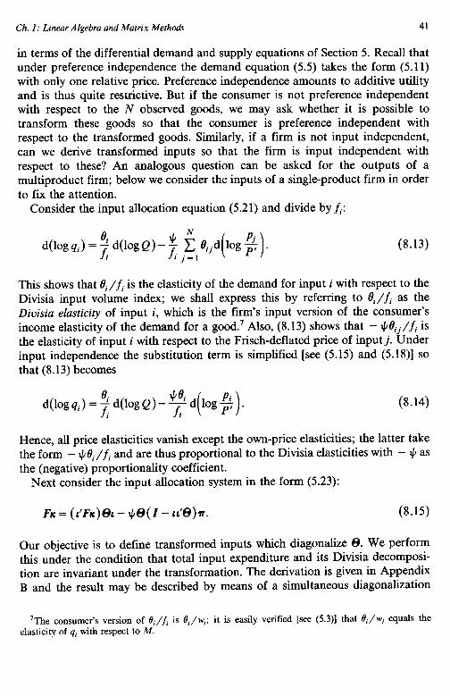
Consider the input allocation equation (5.21) and divide by fi:
d(lOg qi) = 2 d(log Q) - z jc, dijd( log F). (8.13)
This shows that 13,/f, is the elasticity of the demand for input i with respect to the Divisia input volume index; we shall express this by referring to 0,/f, as the Divisia elasticity of input i, which is the firm’s input version of the consumer’s income elasticity of the demand for a good.7 Also, (8.13) shows that - J/di,/fi is the elasticity of input i with respect to the Frisch-deflated price of input j. Under input independence the substitution term is simplified [see (5.15) and (5.18)] so that (8.13) becomes
d(log qi) = 4 d(log Q) - 4 d( log $ ) . I I
(8.14)
Hence, all price elasticities vanish except the own-price elasticities; the latter take the form - J/0,/f, and are thus proportional to the Divisia elasticities with - I/J as the (negative) proportionality coefficient.
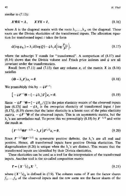
Next consider the input allocation system in the form (5.23):
FK = (C’Eic)& - @(I - d+. (8.15)
Our objective is to define transformed inputs which diagonalize 8. We perform this under the condition that total input expenditure and its Divisia decomposi- tion are invariant under the transformation. The derivation is given in Appendix B and the result may be described by means of a simultaneous diagonalization
‘The consumer’s version of 13,/f, is 0,/w,; it is easily verified [see (5.3)] that O,/ w, equals the elasticity of 4, with respect to M.
42 H. Theil
similar to (7.13):
X%X=A, x’lix = I, (8.16)
where A is the diagonal matrix with the roots X,, . . . , A, on the diagonal. These roots are the Divisia elasticities of the transformed inputs. The allocation equa- tion for transformed input i takes the form
d(logqTi) = &d(logQ)+,d(log$$), (8.17)
where the subscript T stands for “transformed”. A comparison of (8.17) and (8.14) shows that the Divisia volume and Frisch price indexes and J, are all invariant under the transformation.
Recall from (7.11) and (7.13) that any column xi of the matrix X in (8.16) satisfies
(e-AiF)ni=O.
We premultiply this by - $F- ‘:
[-~P-‘e-(-~xi)l]xi=O.
(8.18)
(8.19)
Since - $F-‘8 = [ - JIdij/fi] is the price elasticity matrix of the observed inputs [see (8.13)] and - J’A, is the own-price elasticity of transformed input i [see (8.17)], (8.19) shows that the latter elasticity is a latent root of the price elasticity matrix - #F- ‘8 of the observed inputs. This is an asymmetric matrix, but the hi’s are nevertheless real. To prove this we premultiply (8.18) by F-II2 and write the result as
P- wep- l/2 - hiI) F'/2xi = 0. (8.20)
Since F-‘/263F-1/2 is symmetric positive definite, the Xi’s are all real and positive. Hence, all transformed inputs have positive Divisia elasticities. The diagonahzation (8.20) is unique when the Xi’s are distinct. This means that the transformed inputs are identified by their Divisia elasticities.
These elasticities can be used as a tool for the interpretation of the transformed inputs. Another tool is the so-called composition matrix
T = (X-‘&X-‘, (8.21)
where (X-‘&)4 is defined in (7.9). The column sums of T are the factor shares f,, . . . ,fN of the observed inputs and the row sums are the factor shares of the
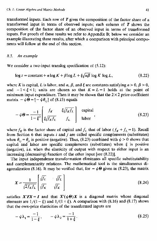
Ch. 1: Linear Algebra and Matrix Methods 43
transformed inputs. Each row of T gives the composition of the factor share of a transformed input in terms of observed inputs; each column of T shows the composition of the factor share of an observed input in terms of transformed inputs. For proofs of these results we refer to Appendix B; below we consider an example illustrating these results, after which a comparison with principal compo- nents will follow at the end of this section.
8.5. An example
We consider a two-input translog specification of (5.12):
logz=constant+cylogK+~logL+~~logK logL, (8.22)
where K is capital, L is labor, and a, p, and [ are constants satisfying LX > 0, /3 > 0, and - 1 < 5 < 1; units are chosen so that K = L = 1 holds at the point of minimum input expenditure. Then it may be shown that the 2 x 2 price coefficient matrix - +@ = [ - #eij] of (8.15) equals
(8.23)
where fK is the factor share of capital and fL that of labor ( fK + fL = 1). Recall from Section 6 that inputs i and j are called specific complements (substitutes) when 19,, = qi is positive (negative). Thus, (8.23) combined with 4 > 0 shows that capital and labor are specific complements (substitutes) when E is positive (negative), i.e. when the elasticity of output with respect to either input is an increasing (decreasing) function of the other input [see (8.22)].
The input independence transformation eliminates all specific substitutability and complementarity relations. The mathematical tool is the simultaneous di- agonalization (8.16). It may be verified that, for - $S given in (8.23), the matrix
(8.24)
satisfies X’I;X = I and that X($&)X is a diagonal matrix whose diagonal elements are l/(1 - 5) and l/(1 + E). A comparison with (8.16) and (8.17) shows that the own-price elasticities of the transformed inputs are
(8.25)

44 H. Theil
Multiple roots occur when 5 = 0, but this is the uninteresting case in which (8.22) becomes Cobb-Douglas, which is in input independent form and thus requires no transformation.
Substitution of (8.24) into (8.21) yields the composition matrix
[fK+m r,+\ir,r,] (T,) T=$ f&&z L
(capital) f&%] CT,).
(labor) (8.26)
The column sums are the factor shares of the observed inputs: fK for capital and fL for labor. The row sums are the factor shares of the transformed inputs: 4 + m for the input T, corresponding to root A, and 4 - JfKf for T2 corresponding to A,. The following is a numerical specification of (8.26), bordered by row and column sums, for fK = 0.2 and fL = 0.8:
Both observed inputs are positively represented in T,, whereas T, is a contrast between labor and capital. When the firm buys more Tz, its operation becomes more labor-intensive, each dollar spent on T2 being equivalent to two dollars worth of labor compensated by one dollar worth of capital services which is given up*
8.6. A principal component interpretation
We return to (8.8) with Z’Z interpreted as n times the matrix of mean squares and products of the values taken by the observed variables. In many applications of the principal component technique, the observed variables have different dimen- sions (dollars, dollars per year, gallons, etc.). This causes a problem, because principal components change in value when we change the units in which the observed variables are measured. To solve this problem, statisticians frequently standardize these variables by using their standard deviations as units. This amounts to replacing Z’Z in (8.8) by D-‘/*Z’ZD-‘I*, where D is the diagonal matrix whose diagonal is identical to .that of Z’Z. Thus, hi of (8.8) is now obtained from the characteristic equation
/D-~/*z~zD-~/* - A,J( = 0. (8.27)

Ch. 1: Linear Algebra and Matrix Methods 45
It is of interest to compare this with
IF-‘/2@F-“2 - h,If = 0, (8.28)
which is the characteristic equation associated with (8.20). In both cases, (8.27) and (8.28), we determine a latent root of a symmetric positive definite matrix (Z’Z or @) pre- and postmultiplied by a diagonal matrix. However, the diagonal elements of F are not identical to those of 8, which is in contrast to D and Z’Z in (8.27). The diagonal elements of F describe the expenditure levels of the inputs (measured as fractions of total expenditure), whereas each diagonal element of 8 describes the change in the demand for an input caused by a change in its Frisch-deflated price.
Thus, while D in (8.27) is directly obtained from Z’Z, the analogous matrix F in (8.28) is unrelated to 8. Why do we have this unrelated F, which describes expenditure levels, in (8.28) and in the simultaneous diagonalization (8.16)? The answer is that the input independence transformation is subject to the constraint that that total input expenditure and its Divisia decomposition remain invariant. We may view this transformation as a cost-constrained principal component transformation. Similarly, when the transformation is applied to the consumer demand system (5.5) or to the output supply system (5.26), it is budget-con- strained in the first case and revenue-constrained in the second. Such constraints are more meaningful from an economic point of view than the standardization procedure in (8.27).
9. The modeling of a disturbance covariance matrix
We mentioned in Section 4 that the disturbance covariance matrix X which occurs in the GLS estimator (4.11) is normally unknown and that it is then usually replaced by the sample moment matrix of the LS residuals. Although this approximation is acceptable under certain conditions when the sample is suffi- ciently large, it is less satisfactory when the number of equations, L in (4.7) and (4.8), is also large. The reason is that B contains many unknowns when L is large or even moderately large. In fact, the sample moment matrix S of the residuals may be singular so that Z-i in (4.11) cannot be approximated by S- ‘. This situation often occurs in applied econometrics, e.g. in the estimation of a fairly large system of demand equations. One way of solving this problem is by modeling the matrix Z. Below we describe how this can be performed when the equations are behavioral equations of some decision-maker.

46 H. Theil
9.1. Rational random behavior
Letx=[x,... xk]’ be the vector of variables controlled by this decision-maker. We write J for the feasible region of x; x for the optimal value of x (X E J); and I( x, i) for the loss incurred when the decision is x rather than X:
/(x,X)=0 ifx=X, >O ifx*X. (9.1)
We assume that the optimal decision X depends on numerous factors, some of which are unknown, so that x is only theoretically optimal in the sense that it is optimal under perfect knowledge. The decision-maker can improve on his ignorance by acquiring information. If he does not do this, we describe the decision made as random with a differentiable density function p,,(x), to be called the prior density function. (The assumption of randomness is justified by the decision-maker’s uncertainty as to the factors determining X.) If he does acquire information, pO( .) is transformed into some other density function p( .) and the amount of information received is defined as
1=/p(x)logzdx,...dx,, J
(9.2)
which is a concept from statistical information theory [see Theil(1967)]. We write c(l) for the cost of information and
i=J,I( x,x)p(x)dx, . ..dx. (9.3)
for the expected loss. If c(Z) and i are measured in the same unit (dollars or any other unit), thepatural solution is the decision distribution with density function p( 0) which minimizes c(I)+ l This p( .) was derived by Barbosa (1975) and the result (see Appendix C) is
p(x)crp,,(x)exp( -v) ifxE J, (9.4)
where a means “is proportional to”, the proportionality coefficient being inde- pendent of x, and c’ is the marginal cost of information dc/dI at the solution (9.4).
Behavior generated by the distribution which density function (9.4) is called rational random behavior. This distribution is determined by three factors: the prior density function p,,(x), the loss function l(x, x), and the marginal cost of
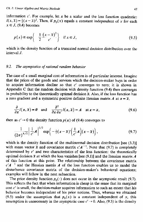
Ch. 1: Lineur Algebra and Matrix Methods 41
information c’. For example, let x be a scalar and the loss function quadratic: 1(x, ~2) =4(x - x)*. Then, if p,,(x) equals a constant independent of x for each x E J, (9.4) becomes
ifxE J, (9.5)
which is the density function of a truncated normal decision distribution over the interval J.
9.2. The asymptotics of rational random behavior
The case of a small marginal cost of information is of particular interest. that the prices of the goods and services which the decision-maker buys
Imagine in order
to acquire information decline so that c’ converges to zero; it is shown in Appendix C that the random decision with density function (9.4) then converges in probability to the theoretically optimal decision Z. Also, if the loss function has a zero gradient and a symmetric positive definite Hessian matrix A at x = X,
x,z)=O and x,x)=A atx=X,
then as c’ + 0 the density function p( x) of (9.4) converges to
&I $4 l”*exP( -4(x-T)'($A)(x-x)}, P-7)
(9-e)
which is the density function of the multinormal decision distribution [see (3.3)] with mean vector 3i and covariance matrix c’A -‘. Note that (9.7) is completely determined by c’ and two characteristics of the loss function: the theoretically optimal decision Z at which the loss vanishes [see (9. l)] and the Hessian matrix A of this function at this point. The relationship between the covariance matrix c’A - ’ and the Hessian matrix A of the loss function enables us to model the disturbance covariance matrix of the decision-maker’s behavioral equations; examples will follow in the next subsection.
The prior density function pO( a) does not occur in the asymptotic result (9.7). This reflects the fact that when information is cheap in the sense that its marginal cost c’ is small, the decision-maker acquires information to such an extent that his behavior becomes independent of his prior notions. Thus, whereas we obtained (9.5) under the assumption that p,(x) is a constant independent of x, this assumption is unnecessary in the asymptotic case c’ + 0. Also, (9.5) is the density

48 H. Theil
function of a truncated normal distribution, but the truncation becomes irrelevant as c’ --, 0. The asymptotic version of (9.5) is the univariate normal density function with mean equal to the theoretically optimal decision x and variance equal to the marginal cost of information c’. The declining variance as c’ + 0 reflects the attractiveness of a more extensive search for the theoretical optimum when information becomes cheaper.
It is of interest to compare the density function (9.7) of the asymptotic normal decision distribution with the asymptotic normal density of a statistical estimator. In fact, it is not difficult to prove that rational random behavior for small c’ is equivalent to large-sample ML estimation of the theoretically optimal decision E, with a large sample interpreted as a small marginal cost of information. The clue for this equivalence is the similarity of the roles played by the Hessian matrix of the loss function and the information matrix in ML theory.
A second statistical comparison is that with Kadane’s (1971) small-u asymp- totics, which consists of an asymptotic series of a multiple (I of the variance of the disturbance of a structural equation. If this equation is a behavioral equation of a decision-maker, Kadane’s approach is equivalent to the asymptotic version of rational random behavior when we identify u with c’.
Another statistical comparison of interest is that with the theorem which states that out of all distributions with range (- co, cc) and a given mean vector and a given covariance matrix, the multinormal distribution has the largest entropy. The link between this theorem and the normal density function (9.7) is the informa- tion definition (9.2); both (9.2) and the entropy are measures from information theory. However, note that the normal density (9.7) is not obtained by imposing a given mean vector and covariance matrix a priori. The mean vector and covari- ante matrix (9.7) are determined by the loss function, apart from the scalar c’.
Yet another statistical comparison is with Bayesian inference. There is consid- erable similarity between the exact (i.e., non-asymptotic) result (9.4) and the Bayesian derivation of the posterior density function of a parameter vector. The occurrence of the prior density function on the right in (9.4) provides one similarity. Another is the presence of c’ (which depends on the information acquired) in the exponent of (9.4); this should be compared with the role of the likelihood function (representing the information obtained from the sample) in the Bayesian formula. A third similarity is the disappearance of the prior density function from the asymptotic result (9.7). In Bayesian analysis, too, the posterior density function is dominated by the likelihood function and is no longer affected by the prior density function when the sample is large. All these similarities reflect the fact that rational random behavior and Bayesian inference both describe learning processes based on acquiring information. Nevertheless, the two theories are not equivalent because of the occurrence of the unknown constant X in (9.4). The likelihood function in Bayesian analysis involves no unknown constants; this function is determined by the parameter vector, which is viewed as random, and

Ch. I: Linear Algebra and Matrix Methods 49
the sample, which is viewed as a set of known constants for the derivation of the posterior density function.
9.3. Applications to demand and supply
When we apply the theory of rational random behavior to the utility-maximizing consumer or the cost-minimizing firm, we must take into consideration that the criterion function is subject to a constraint (a budget or technology constraint). This can be solved by using the constraint to eliminate one of the goods. The consumer’s loss function in (9.4) then involves N - 1 quantities and its derivation from an algebraically specified utility function is straightforward. However, the differential approach provides no such specification so that (9.4) cannot be used; the same holds for the firm because the approach provides no algebraic specifica- tion of the production function. But it is possible to use the asymptotic result (9.7) which requires only the theoretically optimal decision and the Hessian matrix of the loss function. The account which follows is therefore based on the asymptotic decision distribution (9.7) rather than (9.4); this also has the ad- vantage of not requiring a specification of the prior density function pO( -).
Consider the input allocation system in the form (6.1),
~~=(~‘~~)e1--~(I-1L’~)B+e, (9.8)
or in scalar form, using & = 8 = [I$],
(9.9)
where [ ei] = e. The left variable in (9.9) is the i th decision variable of the firm. The right side, excluding ei, is the theoretical optimum of this variable, while .E~ is the random deviation from this optimum which is predicted by the theory of rational random behavior. Since (9.7) implies normality with a mean equal to the theoretically optimal decision, the .si’s are multinormal with zero mean. Their covariance matrix (see Appendix C) is
T(e) = a*(@- 866’8), (9.10)
or in scalar form,
cov(q, Ej) = ayeij - e,e,), (9.11)
where a* is a coefficient which is proportional to the marginal cost of information
50 H. Theil
c’. The covariance matrix (9.10) equals a scalar multiple of the coefficient matrix of P = [d(logpi)] in (9.8) so that the covariance (9.11) is proportional to the substitution effect (specific plus general) of a change in the price of j on the demand for i.
The above result also holds when (9.7) is applied to the consumer; the only modification required is that fi and 4 in (9.9) become wi and - +, respectively [see (5.5)]. Note in particular that the disturbance covariance matrix (9.10) involves only unknown (a’) in addition to 8 which already occurs in the systematic part of the equations. Thus, the implications of rational random behavior are quite strong. We obtain even stronger implications for the demand and supply equa- tions of the multiproduct firm; a brief account follows below.
Recall that when the firm makes m products, the output term of the input demand system (5.15) takes the form (5.25). So, by adding a disturbance &i we obtain:
fid(logqi) = y ~ e,‘gl.d(lOgz,)- ~ ~ B,d(log~)+Ei. r=l j=l
(9.12)
Application of (9.7) yields the result that the si’s of this input demand system are .multinormal with zero means and that their variances and covariances take the same form (9.11) which also holds for the consumer and the single-product firm. Next, by assuming that the firm adjusts its outputs so as to maximize profit, we obtain the output supply system (5.26) which we reproduce with a disturbance E: added:
g,d(logz,) = $* 2 Qd(log$)+e:. s=l
(9.13)
By applying (9.7) we find that the ET’S are multinormal with zero means and the following variance-covariance structure:
cov( ET, E:) = u2+* -e;. Ylc/
(9.14)
Since u2 already occurs in (9.11) for the input demand disturbances, (9.14) provides no further unknowns. In addition, (9.7) implies that the input demand disturbances (the ei’s) are stochastically independent of the output supply dis- turbances (the ET’S). This independence has important implications for statistical inference in demand and supply models; it implies that g,d(log z,.) can be viewed as predetermined in the input demand system (9.12). It is also important for the problem of how to organize the firm in terms of its input and output manage- ment, but such matters are beyond the scope of this chapter.

Ch. I: Linear Algebra and Matrix Methodr
10. The Moore-Penrose inverse
51
A matrix has an inverse only if it is square and nonsingular, but any m x n matrix A of rank r has a unique Moore-Penrose inverse, written A +, which is determined by the following four conditions:
AA+A= A, (10.1)
A+AA+=A+, (10.2)
AA+ and A +A are symmetric. (10.3)
It may be verified that these conditions are satisfied by A + = A - ’ in the special case m = n = r. Our first objective is to prove that A + exists and is unique.8
10.1. Proof of the existence and uniqueness
The uniqueness of A + is established by assuming that conditions (lO.l)-( 10.3) have two solutions, A + = B and A + = C, and verifying the following 16 steps based on (lO.l)-( 10.3):
B = BAB = B(AB)‘= BB’A’= BB’(ACA)‘= BB’A’C’A’
= B(AB)‘(AC)‘= BABAC= BAC= BACAC= (BA)‘(CA)‘C
=~~B~A~c~c=(ABA)~cc=~~c~c=(c~)~c=c~c=c.
Therefore, B = C, which proves that A + is unique when it exists. To prove the existence of A+ we consider first a zero matrix A of order m X n;
then A + equals the n X m zero matrix, which may be verified by checking (lO.l)-(10.3). Next consider a non-zero matrix A so that its rank r is positive. Then A’A is a symmetric positive semidefinite matrix of order n X n and rank r, and it is possible to express A + in terms of the positive latent roots of A’A and the characteristic vectors associated with these roots. Write D for the diagonal r x r matrix which contains the positive roots of A’A on the diagonal and H for an n x r matrix whose columns are characteristic vectors corresponding to these roots. Then (7.7) applied to A’A yields
A’A = HDH’, (10.4)
‘There are other generalized inverses besides the Moore-Penrose inverse, most of which are obtained by deleting one or more of the four conditions. For example, using (10.1) and (10.2) but deleting (10.3) yields the reflexive generalized inverse, which in not unique; see Laitinen and Theil (1979) for an application of this inverse to consumption theory. Monographs on applications of generalized inverses to statistics include Albert (1972), Ben-Israel and Greville (1974), Boullion and Ode11 (197 l), Pringle and Rayner (197 l), and Rao and Mitra (197 1).
52 H. Theil
and the result for A + is
A + = HD-‘H’A’ > (10.5)
which is an n X m matrix of rank r. To verify (10.5) we introduce an n x (n - r) matrix K whose columns are
characteristic vectors of A’A corresponding to the zero roots:
A’AK = 0. (10.6)
The n x n matrix [H K] consists of characteristic vectors of A’A corresponding to all roots and is therefore an orthogonal matrix, which can be expressed in two ways. Premultiplying [H K] by its transpose and equating the product to the unit matrix yields
H’H = I, K’K = I, H’K = 0, (10.7)
while postmultiplying [H K] by its transpose and equating the product to the unit matrix gives
HH’ + KK’ = I. (10.8)
The verification of (10.5) is now a matter of checking conditions (lO.l)-(10.3). Premultiplying (10.5) by A yields AA ’ = AHD- 'H'A', which is symmetric. Next we postmultiply (10.5) by A, A+A = HD-‘H’A’A, and hence in view of (10.4) and (10.7), A +A = HD- ‘H’HDH’ = HH’, which is also symmetric. We postmulti- ply this by (10.5):
A +AA + = HH’HD-‘H’A’= HD- ‘H’A’= A +,
which confirms (10.2). Finally, we postmultiply AA+ = AHD-‘H’A’ by A:
AA+A= AHD-‘H’A’A= AHD-‘H’HDH’= AHIT= A.
To verify the last step, AHH’ = A’, we premultiply (10.6) by K’, which gives (AK)‘AK = 0 or AK = 0. Therefore, AKK’= 0 so that premultiplication of (10.8) by A yields AHH’ = A.
10.2. Special cases
If A has full column rank so that (A'A)- ’ exists, A + = (A'A)- 'A', which may either be verified from (10.4) and (10.5) for r = n or by checking (lO.l)-( 10.3). We may thus write the LS coefficient vector in (2.8) as b = X+y, which may be

Ch. I: Linear Algebra and Matrix Methods 53
viewed as an extension of b = X- ‘y in the special case of a square non-singular X (as many regressors as observations).
If A is a symmetric n X n matrix of rank r, then
A= ; Ai.&, i=l
(10.9)
where A,,..., A, are the non-zero latent roots of A and x,, . . . ,xr are characteristic vectors associated with these roots. Also, Axi = 0 and A +xi = 0 for i = r + 1,. . . , n, where x T+, , . . . ,x, are characteristic vectors of A corresponding to the zero roots. Thus, if A is symmetric, A+ has characteristic vectors identical to those of A, the same number of zero roots, and non-zero roots equal to the reciprocals of the non-zero roots of A. The verification of these results is again a matter of checking (lO.l)-(10.3) and using x[x, = aij. Since a symmetric idempotent matrix such as M in (2.11) has only zero and unit roots, it thus follows as a corollary that such a matrix is equal to its own Moore-Penrose inverse.
10.3. A generalization of Aitken’s theorem
We return to the linear model (2.7), reproduced here:
y=Xp+&. (10.10)
As before, we assume that X is an n X K matrix of rank K consisting of non-stochastic elements and that E has zero expectation, but we now assume that the covariance matrix of E takes the singular form u * V, the n X n matrix V having rank r -C n. Hence, the Aitken estimator (2.13) does not exist, but is seems reasonable to ask whether
/!I= (X’v+x)_‘X’v+y (10.11)
exists and is a best linear unbiased estimator of /3. It will appear that each of these properties (the existence and the best linear unbiasedness) requires a special condition involving both V and X.
The matrix V is comparable to A’A in (10.4) and (10.6) in that both are symmetric positive semidefinite n x n matrices of rank r. Therefore, we can apply (10.4) and (10.6) to V rather than A'A :
V = HDH’, (10.12)
VK=O, (10.13)

54 H. Theil
where D is now the r X r diagonal matrix with the positive latent roots of V on the diagonal, H is an n X r matrix whose columns are characteristic vectors of V corresponding to these roots, and K is an n x (n - r) matrix consisting of characteristic vectors of V that correspond to the zero roots. The results (10.7) and (10.8) are also valid in the present interpretation. In addition, (10.9) and (10.12) imply
V+ = HD-‘H’. (10.14)
Our strategy, similar to that of the proof of Aitken’s theorem in Section 7, will be to premultiply (10.10) by an appropriate matrix so that the transformed disturbance vector has a scalar covariance matrix. We select D-‘12H’, where D-‘12 is the diagonal matrix with the reciprocals of the positive square roots of the diagonal elements of D in the diagonal:
D- 1/2Hry = (D- ‘/“H’X)j3 + D- ‘12H’e.
The covariance matrix of D-‘12H’e is
(10.15)
where the last step is based on H’VH = D, which is obtained by premultiplying (10.12) by H’ and postmultiplying by H and using H’H = I [see (10.7)]. Since D-‘12H’e thus has a scalar covariance matrix, let us apply LS to (10.15). Assuming that H’X and hence D- ‘/2H’X have full column rank, we find the following estimator of j3:
(D-t/2Hfx)+D-t/2Hry= (x’HD-~H’x)-‘x’HD-~H’~.
This is indeed identical to (10.11) in view of (10.14).
(10.16)
Two considerations are important for the appraisal of this procedure. First, we assumed that HIX has full column rank; if the rank is smaller, the matrix product in parentheses on the right in (10.16) is singular so that (10.11) does not exist. Therefore, a necessary and sufficient condition for the existence of the estimator (10.11) is that H’X have maximum rank, where H consists of r characteristic vectors of V corresponding to the positive roots. Secondly, we obtained (10.15) by premultiplying (10.10) by D-‘/2H’, which reduces the number of observations from n to r. We can recover the “missing” n - r observations by premultiplication by K’, yielding K’y = K’Xj3 + K’E. The covariance matrix of K’e is a2K’VK = 0 [see (10.13)] so that K’e vanishes with unit probability. Therefore,
K’y = K’Xfi,
which amounts to a linear constraint on j3 unless K’X = 0.
(10.17)

Ch. 1: Linear Algebra and Matrix Methods 55
To clarify this situation, consider the following example for K = 1, n = 3, and r = 2:
X=[# V=[i i ;], H=[i 81, K=[;]. (10.18)
Here X has full column rank but H’X = 0 so that the matrix product in parentheses on the right in (10.16) is singular; in fact, the underlying equation (10.15) does not contain j? at all when H’X = 0. Thus, the estimator (10.11) does not exist, but in the case of (10.18) it is nevertheless possible to determine /3 (a scalar in this case) exactly! The reason is that (10.18) implies K’y = y3 and K’X = 1 so that (10.17) states that y, equals the parameter. Ultimately, this results from the zero value of the third diagonal element of V in (10.18) and the non-zero third element of X.
Under the assumptions stated in the discussion following eq. (lO.lO), the estimator (10.11) exists when H’X has full column rank and it is a best linear unbiased estimator of B when K’X = 0 [so that (10.17) is not a real constraint on /3]. A proof of the latter statement follows in the next paragraph. If K’X is a non-zero matrix, (10.17) is a linear constraint on j3 which should be incorporated in the estimation procedure; see Theil (1971, sec. 6.8).
We can write any linear estimator of /LI as
s = [A +(X’Y+X)-‘X’V+] y, (10.19)
where A is some K x n matrix consisting of non-stochastic elements. By substitut- ing Xfi + e for y in (10.19) and taking the expectation we find that the unbiased- ness of B requires
AX=O, (10.20)
so that j? - /Cl = [A + (X’V+X)- ‘X’V+ ]e and the covariance matrix of fi equals
V(j?) =&[A +(X’V+X)-‘XV+]+‘+ V+x(x’V+x)-‘I. (10.21)
For A = 0 we have B = B in view of (10.19). Thus, using V+ IV+ = V+ and (10.21), we obtain:
V(B) = 02(x’v+x)-‘, (10.22)
which is a generalization of (2.14). The excess of (10.21) over (10.22) equals a multipleo2ofAVA’+AVV+X(X’VfX)-‘+(X’VtX)-’X’V+VA’.ButAVV’X =0 so that ‘V(B)-‘V(b)=a2AVA’, which is positive semidefinite and thus
56 H. Theil
establishes that B is best linear unbiased. To verify that A VV+X is a zero matrix we use (10.12) and (10.14) in
VV+ = HDH’HD- ‘H’ = HH’ = I - KK’,
where the last two steps are based on (10.7) and (10.8). So, using (10.20) and K’X = 0 also, we have
AVV+X=AX-AKK’X=O-O=O.
The matrix ?r( b)- Ir( /) = u *A VA’ is obviously zero when we select A = 0, but it may also be zero for A * 0 when V is singular, which suggests that there is no unique best linear unbiased estimator of 8. This is not true, however; if the estimator (10.11) exists, i.e. if H’X has full column rank, it is the unique best linear unbiased estimator of /3 when K’X = 0. The reason is that A VA’ = 0 is equivalent to &[Ae(Ae)‘] = 0 so that Ae is a zero vector with unit probability. Using (10.20) also, we obtain Ay = A(X,L? + e) = 0, which in conjunction with (10.19) shows that the best hnear unbiased estimator of /3 must be of the form (10.1 l), even though A may be a non-zero matrix.
10.4. Deleting an equation from an allocation model
The Moore-Penrose inverse can also be conveniently used to prove that when we estimate an N-equation allocation system such as (6.1), we can simply delete one of the N equations (it does not matter which). The clue is the fact that each equation can be obtained by adding the N - 1 others. We prove this below for an allocation system which is linear in the parameters. The strategy of the proof will be to start with GLS estimation of N - 1 equations with a non-singular dis- turbance covariance matrix, followed by adding the deleted equation (so that the disturbance covariance matrix becomes singular), and then proving that the resulting estimator (10.11) is identical to the original GLS estimator.
We can formulate the problem in the following more general way. Lety = X,8 + E have a non-singular covariance matrix v(e) = a* V of order n X n. We premultiply by a matrix B of order (n + n’) x n and rank n:
By = BXB + Be. (10.23)
For example, take B’ = [I C], which means that we add to the original n observations n’ linear combinations of these observations. The covariance matrix of Be takes the singular form a*BVB’. Thus, the matrix V of the previous subsection becomes B VB’ here, while X becomes BX. We conclude that condition
Ch. I: Linear Algebra and Matrix Methods 51
K’X = 0 is now K’( BX) = 0, where K is a matrix whose n’ columns are character- istic vectors of B VB’ corresponding to the zero roots: (B VB’)K = 0 and K’K = I. Evidently, a sufficient condition for K is B’K = 0 and K’K = I. Such a K can be obtained as a matrix whose columns are characteristic vectors of the idempotent matrix Z - B( B'B)- 'B' corresponding to the unit roots:
[I- B(B~B)-'B~]K=K.
The GLS estimator (10.11) of /3 in (10.23) is then
[x'B'(BVB')+BX]-'X'B'(BVB')+B~. (10.24)
This is identical to (XV-‘X)) ‘X’V-‘y, and hence to the GLS estimator ob- tained from the original n observations, because
B'(BVB')+B=V-',
which follows from BVB'(BVB')+BVB'= BVB' [see (lO.l)] premultiplied by V- ‘( B’B)- ‘B’ and postmultiplied by B( B'B)- ‘VP ‘. It is unnecessary to check the condition that H'(BX) has full column rank, H being a matrix whose n columns are characteristic vectors of BVB’ corresponding to the positive roots. The reason is that the estimator (10.24) would not exist if the condition were not satisfied, whereas we know that (10.24) equals (XV- IX)- ‘XV ‘y.
Appendix A: Linear independence and related topics
Consider a matrix Y= [Q,... u,] and a linear combination Vc of its n columns. The vectors 0 ,, . . . ,v,, are said to be linearly independent if Vc = 0 implies c = 0, i.e. if there exists no non-trivial linear combination of the vi’s which is a zero vector. For example, the columns of the 2x2 unit matrix are linearly independent because
c,[~]+~z[~]=[~~]=[~] implies c,=c,=O,
but v, = [l 01’ and vz = [2 01’ are not linearly independent because c,v, + czq = 0 if (for example) c, = 2 and c2 = - 1.
For any m X n matrix A the column rank is defined as the largest number of linearly independent columns, and the row rank as the largest number of linearly independent rows. It can be shown that these two ranks are always equal; we can thus speak about the rank r of A, which obviously satisfies r < m, n. If all

58 H. Theil
columns (rows) of A are linearly independent, A is said to have full column (row) rank. For any A, the ranks of A, A’, A’A, and AA’ are all equal. Also, the rank of AB is at most equal to the rank of A and that of B. For example,
which illustrates that the rank of AB may be smaller than both that of A and that of B. (A zero matrix has zero rank.) If A is square (n x n) and has full rank (r = n), it is called non-singular and its inverse A-’ exists.
For any vector u = [q], its length is defined as the positive square root of v’v = xi vi”. If v’v = 1, v is said to have unit length. The inner product of two vectors v = [vi] and w = [ wi] consisting of the same number of elements is defined as D’W = xi viwi. If V’W = 0, u and w are called orthogonal vectors.
A square matrix X which satisfies X’ = X- ’ is called an orthogonal matrix. Premultiplication of X’ = X- ’ by X gives XX’ = I, which shows that each row of X has unit length and that any two rows of X are orthogonal vectors. Postmulti- plication of X’ = X- ’ by X gives X’X = I so that each column of X (each row of X’) also has unit length and any two columns of X are also orthogonal vectors.
Appendix B: The independence transformation
The independence transformation is based on three axioms, the first being the invariance of total expenditure. Let a dollar spent on observed inputj result in rjj dollars spent on transformed input i, so that the expenditure on i equals cjrijpjqj and the total expenditure on all transformed inputs equals cj(&rjj)pjqj, which must be identical to cjpjqj because of the invariance postulated. Therefore, c,rij = 1 for eachj, or
r’R = I’, (B.1)
where R = [rjj]. By dividing the expenditure cjrijfjqj on transformed input i by total expenditure C (which is invariant) we obtam the factor share fTi of this input. Therefore, f Tj = cjrijjfi, or
F,t = RFL, 03.2)
where FT is the diagonal factor share matrix of the transformed inputs. The second axiom states that the logarithmic price and quantity changes of the
transformed inputs are linear combinations of their observed counterparts, mT = S,s and K= = S*K, so that the associated Divisia indexes are invariant. The Divisia

Ch. I: Linear Algebra and Matrix Methods 59
volume index is d(logQ) = I’FK and its transformed counterpart is dFTtcT = dF&u = r’F(R’S,)tt [see (B.2)]. Thus, the invariance of this index requires R’S, = I or S, = (R’)- ‘. We can proceed similarly for the price index L’F~, which yields the same result for S,, so that the price and quantity transformations use the same matrix, or = Sr and or = SK, where S = (R’)-‘. See remark (3) below for the case of a singular R.
The third axiom diagonalizes 8. We premultiply (8.15) by R, which yields RFtc = RFR’Su = RFR’K, on the left because R’S = I and SK = K=. When we proceed similarly on the right and use (B.l) also, we obtain:
RFR~U, = ( ~FK)( RBR$ - +R~R’[I - d( R~R’)] 7+, (B.3)
which is an allocation system of the same form as (8.15), with logarithmic price and quantity changes or and K=, p rovided RFR’ on the left equals the diagonal factor share matrix FT. The new normalized price coefficient matrix is R@R’, which occurs in the same three places in (B.3) as 8 does in (8.15). [The matrix R8R’ is indeed normalized because ~‘R@R’L = 4% = 1 follows from (B. l).] There- fore, RFR’ = FT and R8R’ = diagonal are the conditions under which (B.3) is an input independent allocation system. These are two conditions on R, which must satisfy (B. 1) also.
We proceed to prove that
R = (x-‘6),x’ (B.4)
satisfies these three conditions, with X defined in (8.16) and (X’r), in (7.9). First, 1’R = I’ is true for (B.4) in view of (7.10). Secondly, RFR’ = (X- ‘L)~X’FX( X- 16)A = (X- ‘6): [see (8.16)] so that
RFR’ = FT = ( X- ‘t): = diagonal. (B.5)
Thirdly, using 8 = (Xl)- ‘AX- ’ [see (8.16)], we have R8R’ = (X- ‘&):A, which is diagonal. So, using (B.5) also and premultiplying (B.3) by (RFR')- ’ = ( X-‘t)i2, we obtain:
which is the matrix version of (8.17). The expression which is subtracted in parentheses in the substitution term of (B.6) represents the deflation by the Frisch price index, which is invariant. To prove this we note that the marginal share vector of the transformed inputs equals R86 = RB in view of the real-income term in (B.3) and R’L = c; the invariance of the Frisch index then follows from (Rt?J)‘s, = &R’Sa = (9%.

60 H. Theif
The expenditure on transformed input i equals rijpjqj dollars insofar as it originates with observed input j. By dividing this amount by total expenditure C we obtain rijfi, which is thus the factor share of transformed input i insofar as it originates with observed input j. This rjjfj is an element of the matrix RF, to be written T:
T = RF= (X-‘&X-‘, (B.7)
where the last step is based on (B.4) and F = (X’)-‘X-’ [see (8.16)]. Postmulti- plication of (B.7) by L gives TL = RFL = F+ [see (B.2)]; hence the row sums of T are the factor shares of the transformed inputs. Also, L’T = L’RF = dF, so that the column sums of T are the factor shares of the observed inputs. Note that (B.7) and its row and column sums confirm the results on the composition matrix. Note further that F = (X’)- ‘X- ’ and 8 = (Xl)- 'AX- ’ [see (8.16)] imply that the price elasticity matrix - #F-‘8 in (8.19) equals - #XAX-‘. So, using (B.7) also, we have
T(- $F-‘e) = - I/J(X-‘&AX-’ = - $A(X-l&X-’ = - ,j,AT_
Combining the first and last member yields ti( - #F'- ‘S) = - GAiti, where tl is the i th row of T, or
t;[-#F-‘e-(-J/x,)1]=&
Therefore, each row of the composition matrix is a characteristic row vector of the (asymmetric) price elasticity matrix of the observed inputs.
We conclude with the following remarks.
(1) Although the solution (B.4) satisfies all three conditions, it is not unique. However, it may be shown that this solution is unique up to premultiplication by an arbitrary permutation matrix; such a multiplication affects only the order in which the transformed inputs are listed.
(2) We proved in the second paragraph that the price and quantity transforma- tions take the form or = Ss and icr = SK, where S = (R’)-‘. It thus follows from (B.l) that S-‘I = L or SL = L. Therefore, when the prices of the observed inputs change proportionately, B being a scalar multiple k of I, the price of each transformed input changes in the same proportion: rr = S(kr) = kSr = kb. The quantities have the same desirable property.
(3) It follows from (B.4) that R is singular when (X-II), contains a zero diagonal element, and from (B.5) that this implies a zero factor share of one of the transformed inputs. In that case S = (R’)-’ does not exist. The simplest way to interpret this situation is by means of a perturbation of the firm’s technology so
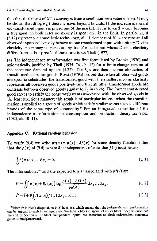
Ch. I: Linear Algebra and Matrix Methods 61
that the i th element of X- ‘I converges from a small non-zero value to zero. It may be shown that d(logpri) then increases beyond bounds. If the increase is toward cc, transformed input i is priced out of the market; if it is toward - co, i becomes a free good; in both cases no money is spent on i in the lit. In particular, if (5.12) represents a homothetic technology, N - 1 elements of X- ‘1 are zero and all observed inputs collectively behave as one transformed input with unitary Divisia elasticity; no money is spent on any transformed input whose Divisia elasticity differs from 1. For proofs of these results see Theil (1977).
(4) The independence transformation was first formulated by Brooks (1970) and axiomatically justified by Theil (1975-76, ch. 12) for a finite-change version of the consumer demand system (5.22). The XI’s are then income elasticities of transformed consumer goods. Rossi (1979a) proved that when all observed goods are specific substitutes, the transformed good with the smallest income elasticity represents all observed goods positively and that all other transformed goods are contrasts between observed goods similar to Tz in (8.26). The former transformed good serves to satisfy the consumer’s wants associated with the observed goods in the least luxurious manner; this result is of particular interest when the transfor- mation is applied to a group of goods which satisfy similar wants such as different brands of the same type of commodity? For an integrated exposition of the independence transformation in consumption and production theory see Theil (1980, ch. 10-11).
Appendix C: Rational random behavior
To verify (9.4) we write p*(x) = p(x)+ Sf(x) for some density function other that the p(x) of (9.4), where S is independent of x so that f( .) must satisfy
I() f x dx,...dx,=O. J
The information I* and the expected loss I” associated with p*( *) are
I*= JIPb)+sf(~)ll% J P(x)+sf(x) dx
POW , . ..dxk.
I*=i+S(l(x,x)f(x)dx,...dx,, JJ
(C-2)
‘When 8 is block-diagonal, so is X in (8.16), which means that the independence transformation can be applied to each block separately. We have a block-diagonal 8 under block independence. See the end of Section 6 for block independent inputs; the extension to block independent consumer goods is straightforward.
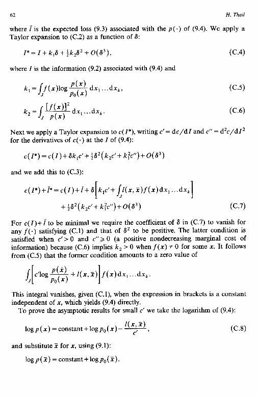
62 H. Theil
where i is the expected loss (9.3) associated with the p( -) of (9.4). We apply a Taylor expansion to (C.2) as a function of 8:
I* = I + k,S + +k,S2 + 0( S3),
where I is the information (9.2) associated with (9.4) and
(C-4)
P(X) k, = ~f(x)log PO(x) dx, --.dx/c,
[f WI’ k, =J, p(x) dx, . ..dx..
(C.5)
(C-6)
Next we apply a Taylor expansion to c( I*), writing c’ = de/d I and c” = d2c/d I 2 for the derivatives of c( *) at the I of (9.4):
and we add this to (C.3):
c(l*)+!*=c(1)+,_+6 k,c’+~(x,r)f(x)dx,...dx, I 1
+$S2(k2c’+k;c”)+0(63) (c.7)
For c(l)+ I to be minimal we require the coefficient of 6 in (C.7) to vanish for any f(e) satisfying (C.1) and that of a2 to be positive. The latter condition is satisfied when c’ > 0 and c” > 0 (a positive nondecreasing marginal cost of information) because (C.6) implies k, > 0 when f(x) f 0 for some x. It follows from (C.5) that the former condition amounts to a zero value of
c’log$$+l(r,E) f(x)dx,...dx,. I
This integral vanishes, given (C.l), when the expression in brackets is a constant independent of x, which yields (9.4) directly.
To prove the asymptotic results for small c’ we take the logarithm of (9.4):
f(x, x) logp(x) =constant+logpO(r)-7, c-4
and substitute X for x, using (9.1):
logp(X) =constant+logp,(Z).

Ch. I: Linear Algebra and Matrix Methocls 63
Since the constants in these equations are equal, subtraction yields
log-p(x)= log Pcm + G, 4 - - P(X) POW c’ . (C.9)
It follows from (9.1) that as c’ + 0 the last term increases beyond bounds for any x t X, so that the same holds for p( F)/p( x) on the left. Hence, as c’ --, 0 the density p(x) becomes zero for each x * ? and the random decision with density function (9.4) thus converges in probability to X.
To verify the asymptotic distribution (9.7), we define
u=+(x-r), (C.10)
so that I(x, X) = I(% + @u, x). We apply a Taylor expansion to I(x, X)/C’, using (9.6):
=+u’Au+o(@). (c.11)
We assume that p,(x) is positive and differentiable around 5. Hence, we can apply a Taylor expansion to log p,,(x) and write it as log po( 2) plus a linear remainder term in x - X. Therefore, in view of (C.lO),
logP,(x) = logP,w+o(~),
which in conjunction with (C.8) and (C. 11) shows that log p( x) equals a constant minus fu’Au plus two remainder terms which both converge to zero as c’ + 0. The result (9.7) is then obtained by substitution from (C.10) for v in $+Au.
We obtain (9.11) from (9.7) by using the budget or technology constraint to eliminate one of the decision variables from the criterion function. Let these variables be the quantities bought by the consumer; it was shown by Theil (1975-76, sec. 2.6-2.7) that (9.7) then yields variances and covariances of the form
cov(qi,qj) = -k Xu’j- i
h aq. &lj I-
i aii/aMaMaikf 7 (C.12)
where k b 0 is proportional to the marginal cost of information c’. A comparison of (C.12) with (3.12) shows that cov(q,, qj) is proportional to the substitution

64 H. Theil
component (specific plus general) of aqi/aFj. We obtain (9.11) from (C.12) by rearrangements required by the left variable m (5.5).
The results (9.11) and (9.14) for the multiproduct firm and the stochastic independence of the input demand disturbances and the output supply dis- turbances were derived by Laitinen and Theil (1978). Reference should also be made to Bowman et al. (1979) and to Rossi (1979b, 1979~) for a comparison of rational random behavior and search theory.
References
Aitken, A. C. (1935) “On Least Squares and Linear Combination of Observations”, Proceedings of the Royal Society of Edinburgh, 55, 42-48.
Albert, A. (I 972) Regression and the Moore- Penrose Pseudoinverse. New York: Academic Press. Barbosa, F. de H. (1975) “Rational Random Behavior: Extensions and Applications”, Doctoral
dissertation, The University of Chicago. Barten, A. P. (1964) “Consumer Demand Functions under Conditions of Almost Additive Prefer-
ences”, Econometrica, 32, 1-38. Barten, A. P. (1977) “The Systems of Consumer Demand Functions Approach: A Review”,
Econometrica, 45, 23-5 I. Barten, A. P. and E. Geyskens (1975) “The Negativity Condition in Consumer Demand”, European
Economic Review, 6, 227-260. Bellman, R. (1960) Introduction to Matrix Analysis. New York: McGraw-Hill Book Company. Ben-Israel, A. and T. N. E. Greville (1974) Generatized Inverses: Theoty and Apphcations. New York:
John Wiley and Sons. Boullion, T. L. and P. L. Ode11 (1971) Generalized Inverse Matrices. New York: John Wiley and Sons. Bowman, J. P., K. Laitinen and H. Theil (1979) “New Results on Rational Random Behavior”,
Economics Letters, 2, 201-204. Brooks, R. B. (1970) “Diagonalizing the Hessian Matrix of the Consumer’s Utility Function”,
Doctoral dissertation, The University of Chicago. Brown, A. and A. Deaton (1972) “Surveys in Applied Economics: Models of Consumer Behaviour”,
Economic Journal, 82, 1145- 1236. Dhrymes, P. J. (1978) Mathematics for Econometrics. New York: Springer-Verlag. Divisia, F. (1925) “L’indice monetaire et la theorie de la monnaie”, Revue d’Economie Politique, 39,
980- 1008. Frisch, R. (1932) New Methodr of Measuring Marginal Utility. Tiibingen: J. C. B. Mohr. Goldberger, A. S. (1959) Impact Multipliers and Dynamic Properties of the Klein -Goldberger Model.
Amsterdam: North-Holland Publishing Company. Graybill, F. A. (1969) Introduction to Matrices with Applications in Statistics. Belmont, Cal.: Wads-
worth Publishing Company. Hadley, G. (1961) Linear Algebra. Reading, Mass.: Addison-Wesley Publishing Company. Hall, R. E. (1973) “The Specification of Technology with Several Kinds of Output”, Journal of
Political Economy, 81, 878-892. Houthakker, H. S. (I 960) “Additive Preferences”, Econometrica, 28, 244-257; Errata, 30 (1962) 633. Kadane, J. B. (1971) “Comparison of k-Class Estimators when the Disturbances are Small”,
Econometrica, 39, 723-737. Laitinen, K. (1980) A Theoty of the Multiproduct Firm. Amsterdam: North-Holland Publishing
Company. Laitinen, K. and H. Theil (1978) “Supply and Demand of the Multiproduct Firm”, European
Economic Review, 11, 107- 154. Laitinen, K. and H. Theil (1979) “The Antonelli Matrix and the Reciprocal Slutsky Matrix”,
Economics Letters, 3, 153- 157.
Ch. 1: Linear Algebra and Matrix Methods 65
Phlips, L. (I 974) Applied Consumption Analysis. Amsterdam: North-Holland Publishing Company. Pringle, R. M. and A. A. Rayner (1971) Generalized Inverse Matrices with Applications to Statistics.
London: Charles Griffin and Co. Rao, C. R. and S. K. Mitra (1971) Generalized Inverse of Matrices and Its Applications. New York:
John Wiley and Sons. Rossi, P. E. (1979a) “The Independence Transformation of Specific Substitutes and Specific Comple-
ments”, Economics Letters, 2, 299-301. Rossi, P. E. (1979b) “The Cost of Search and Rational Random Behavior”, Economics Letters, 3, 5-8. Rossi, P. E. (1979~) “Asymptotic Search Behavior Based on the Weibull Distribution”. Economics
Letters, 3. 21 I-213. Theil, H. (1967) Economics and Information Theory. Amsterdam: North-Holland Publishing Company. Theil. H. (1971) Princioles of Econometrics. New York: John Wiley and Sons. Theill H. ‘(1975-76) Theo& and Measurement of Consumer Demand, 2 ~01s. Amsterdam: North-
Holland Publishing Company. Theil, H. (1977) “The Independent Inputs of Production”, Econometrica, 45, 1303-1327. Theil, H. ( 1980) The System Wide Approach to Microeconomics. Chicago: University of Chicago Press. Theil, H. and K. W. Clements (1980) “Recent Methodological Advances in Economic Equation
Systems”, American Behavioral Scientist, 23, 789-809. Theil, H. and K. Laitinen (1979) “Maximum Likelihood Estimation of the Rotterdam Model under
Two Different Conditions”, Economics Letters, 2, 239-244. Zellner, A. (1962) “An Efficient Method of Estimating Seemingly Unrelated Regressions and Tests for
Aggregation Bias”, Journal of the American Statistical Association, 57, 348-368.