Lin, Chun and Masey, Nicola and Wu, Hao and Jackson, Mark and

Carruthers, David J. and Reis, Stefan and Doherty, Ruth M. and

Beverland, Iain J. and Heal, Mathew R. (2017) Practical field calibration of

portable monitors for mobile measurements of multiple air pollutants.

Atmosphere, 8 (12). ISSN 2073-4433 ,

http://dx.doi.org/10.3390/atmos8120231

This version is available at https://strathprints.strath.ac.uk/62603/

Strathprints is designed to allow users to access the research output of the University of

Strathclyde. Unless otherwise explicitly stated on the manuscript, Copyright © and Moral Rights

for the papers on this site are retained by the individual authors and/or other copyright owners.

Please check the manuscript for details of any other licences that may have been applied. You

may not engage in further distribution of the material for any profitmaking activities or any

commercial gain. You may freely distribute both the url (https://strathprints.strath.ac.uk/) and the

content of this paper for research or private study, educational, or not-for-profit purposes without

prior permission or charge.

Any correspondence concerning this service should be sent to the Strathprints administrator:

strathprints@strath.ac.uk

The Strathprints institutional repository (https://strathprints.strath.ac.uk) is a digital archive of University of Strathclyde research

outputs. It has been developed to disseminate open access research outputs, expose data about those outputs, and enable the

management and persistent access to Strathclyde's intellectual output.

atmosphere

Article

Practical Field Calibration of Portable Monitors forMobile Measurements of Multiple Air Pollutants

Chun Lin 1, Nicola Masey 2, Hao Wu 1, Mark Jackson 3, David J. Carruthers 3, Stefan Reis 4,5 ID ,

Ruth M. Doherty 6, Iain J. Beverland 2 and Mathew R. Heal 1,* ID

1 School of Chemistry, University of Edinburgh, Joseph Black Building, David Brewster Road,

Edinburgh EH9 3FJ, UK; c.lin@ed.ac.uk (C.L.); hao.wu@ricardo.com (H.W.)2 Department of Civil & Environmental Engineering, University of Strathclyde, James Weir Building,

75 Montrose Street, Glasgow G1 1XJ, UK; nicola.masey@ricardo.com (N.M.);

iain.beverland@strath.ac.uk (I.J.B.)3 Cambridge Environmental Research Consultants Ltd., 3 King’s Parade, Cambridge CB2 1SJ, UK;

mark.jackson@cerc.co.uk (M.J.); david.carruthers@cerc.co.uk (D.J.C.)4 NERC Centre for Ecology & Hydrology, Bush Estate, Penicuik EH26 0QB, UK; srei@ceh.ac.uk5 European Centre for Environment and Health, University of Exeter Medical School, Knowledge Spa,

Royal Cornwall Hospital, Truro TR1 3HD, UK6 School of GeoSciences, University of Edinburgh, Crew Building, Alexander Crum Brown Road,

Edinburgh EH9 3FF, UK; ruth.doherty@ed.ac.uk

* Correspondence: m.heal@ed.ac.uk; Tel.: +44-131-650-4764

Received: 20 October 2017; Accepted: 18 November 2017; Published: 23 November 2017

Abstract: To reduce inaccuracies in the measurement of air pollutants by portable monitors it is

necessary to establish quantitative calibration relationships against their respective reference analyser.

This is usually done under controlled laboratory conditions or one-off static co-location alongside

a reference analyser in the field, neither of which may adequately represent the extended use

of portable monitors in exposure assessment research. To address this, we investigated ways of

establishing and evaluating portable monitor calibration relationships from repeated intermittent

deployment cycles over an extended period involving stationary deployment at a reference site,

mobile monitoring, and completely switched off. We evaluated four types of portable monitors:

Aeroqual Ltd. (Auckland, New Zealand) S500 O3 metal oxide and S500 NO2 electrochemical; RTI

(Berkeley, CA, USA) MicroPEM PM2.5; and, AethLabs (San Francisco, CA, USA) AE51 black carbon

(BC). Innovations in our study included: (i) comparison of calibrations derived from the individual

co-locations of a portable monitor against its reference analyser or from all the co-location periods

combined into a single dataset; and, (ii) evaluation of calibrated monitor estimates during transient

measurements with the portable monitor close to its reference analyser at separate times from the

stationary co-location calibration periods. Within the ~7 month duration of the study, ‘combined’

calibration relationships for O3, PM2.5, and BC monitors from all co-locations agreed more closely on

average with reference measurements than ‘individual’ calibration relationships from co-location

deployment nearest in time to transient deployment periods. ‘Individual’ calibrations relationships

were sometimes substantially unrepresentative of the ‘combined’ relationships. Reduced quantitative

consistency in field calibration relationships for the PM2.5 monitors may have resulted from generally

low PM2.5 concentrations that were encountered in this study. Aeroqual NO2 monitors were sensitive

to both NO2 and O3 and unresolved biases. Overall, however, we observed that with the ‘combined’

approach, ‘indicative’ measurement accuracy (±30% for O3, and ±50% for BC and PM2.5) for 1 h

time averaging could be maintained over the 7-month period for the monitors evaluated here.

Keywords: air pollution sensor; air quality; O3; NO2; PM2.5; black carbon; personal exposure

Atmosphere 2017, 8, 231; doi:10.3390/atmos8120231 www.mdpi.com/journal/atmosphere

Atmosphere 2017, 8, 231 2 of 19

1. Introduction

Large public health burdens are associated with human exposure to nitrogen dioxide (NO2), ozone

(O3), and particulate matter (PM) in urban areas [1–3]. The ambient concentrations of these pollutants

are routinely monitored to assess compliance with air quality legislation and the effectiveness of air

pollution mitigation measures. The black carbon (BC) component of PM is also often monitored,

although not specifically for regulatory compliance, as a marker of combustion-related air pollution

and because of its association with adverse health effects [4,5].

These pollutants are usually monitored using automatic ‘reference’ analysers at a small number

of (sometimes only one) fixed sites within urban areas. They are termed reference analysers because of

the instruments used—and the QA/QC processes that are applied to instrument operation, calibration,

and post-processing of output—follow defined protocols, such that final concentration values are, in

principle, traceably correct, within stated uncertainty tolerances, to agreed national or international

standards. In the United Kingdom (UK), these instruments form part of the national Automatic Urban

and Rural Network (AURN, https://uk-air.defra.gov.uk), and similar regional networks. Reference

instruments have high capital and on-going operational costs, and require secured sites with mains

power. As a consequence, there has been considerable interest in the recent emergence of smaller,

battery-operated instruments that can measure a range of air pollutants [6–11]. The lower capital

cost, small size, and low power needs of these instruments have led to their deployment in large

spatial networks [12–14] and in mobile and peripatetic (short periods of deployments at multiple sites)

measurement designs [15–19], including in personal monitoring and ‘citizen science’ contexts [20–23].

Quantitative relationships need to be established between portable air pollution monitor outputs

and their respective reference measurements. Whilst quantitative performance of portable monitors

can be rigorously evaluated under controlled laboratory conditions [22,24–26], it is essential that

monitor performance is also evaluated in ambient deployment [11,25,27]. Most monitor evaluation

studies report data from a single comparison [12,13,20,28–32], including those that are conducted

under the auspices of agency evaluations [27,33–35], although some studies first divide the co-location

data into training and test datasets [36,37].

However, neither laboratory studies nor one-off static co-location adjacent to a reference analyser

represent likely typical ‘field’ usage of these portable monitors. Thus, the aim of this study was

to investigate approaches to the establishment and evaluation of portable monitor vs. reference

calibration relationships for four types of portable monitor (Aeroqual Ltd. (Auckland, New Zealand)

S500 O3 and S500 NO2 monitors, RTI ((Berkeley, CA, USA) MicroPEM PM2.5 monitors, and AethLabs

(San Francisco, CA, USA) microAeth AE51 monitors) under conditions that are realistic of their likely

usage, namely repeated instances over an extended period of intermittent deployment at a reference

site, portable monitoring, and completely switched off. Previous studies have not examined the

repeated usage of portable monitors over a period of several months in the field. Of interest is the

reproducibility of the quantitative relationship between a portable monitor and its respective reference

in a series of fixed-site co-locations, and whether to take a one-off near-in-time fixed-site relationship

as the calibration for a given set of portable measurements, or to pool together a set of fixed-site

calibrations to cover a set of portable measurements. Since it is impractical to compare portable and

reference monitors ‘on the move’ during mobile measurements, studies to evaluate portable monitors

must still resort to comparison of measurements adjacent to fixed-site reference analysers. Thus,

the innovative aspects of this study were: (1) comparison of the accuracy of calibrated estimates

using calibration data from separate co-location periods against reference analysers with estimates

using a single combined calibration dataset of all co-location periods; and, (2) evaluation of portable

monitor calibrations over short periods when the portable monitors were transiently positioned close

to fixed-site reference analysers during mobile measurement campaigns at times separate from the

periods of co-location from which the calibration equations were derived. To the best of our knowledge

these aspects have not been investigated before. The overarching motivation was to gain insight into

Atmosphere 2017, 8, 231 3 of 19

the ‘in field’ quantification of the portable monitor output during routine usage, not on the detail of

the resultant calibrations, which will likely vary according to the particular monitor available.

2. Methods

2.1. Portable Monitors

This study used the following portable monitors.

(i) Two Aeroqual S500 monitors containing electrochemical NO2 sensors (ENW2, range 0–1 ppm)

(www.aeroqual.com), designated ‘Aq1’ and ‘Aq2’.

(ii) Two Aeroqual S500 monitors containing metal-oxide semiconductor O3 sensors (OZU2, range

0–0.15 ppm) (www.aeroqual.com), designated ‘Aq3’ and ‘Aq4’.

(iii) Two RTI MicroPEM PM2.5 monitors (www.rti.org/impact/micropem-sensor-measuring-

exposure-air-pollution) (designated ‘MP586N’ and ‘MP618N’), which detect particles by

converting scattered laser light intensity into a mass concentration of particles. Although optical

scattering is insensitive to particles smaller than about 0.4 µm, particles that are smaller than this

size only make a small contribution to the PM2.5 mass concentration [38].

(iv) Two AethLabs microAeth AE51 monitors (https://aethlabs.com) (designated ‘MA1303’ and

‘MA1204’), which quantify BC from the amount of light absorbed by sampled particulate matter

and application of an extinction parameter to convert optical attenuation into a BC concentration.

The PM2.5 and BC portable monitor measurements are both potentially subject to a source of

uncertainty additional to any error in recording the direct response of the instrument to the ‘analyte’ in

the air stream: a given ambient particle mix may have composition and size distributions, and hence

optical properties, that differ from the particle mix on which the internal factors that convert the optical

measurements into their respective PM2.5 and BC mass concentrations are based. This gives rise to

unquantifiable erroneous values. However, in the case of BC measurement, the same mass extinction

coefficient is also applied in the BC reference analyser.

2.2. Measurement Locations and Schedules

The NO2, O3, and BC portable monitors were repeatedly co-located for a few days at a time

at a UK government Automatic Urban Rural Network (AURN) urban background monitoring site

at Townhead in central Glasgow during February to August 2016 (Table 1). Reference analysers for

NO2, O3, and BC at this site are a Teledyne API200A chemiluminescence analyser, a Thermo 49i UV

absorbance analyser, and a Magee Scientific AE22 Aethalometer respectively. The PM2.5 portable

monitors were co-located at the St. Leonard’s urban background AURN monitoring site in central

Edinburgh, which houses a Thermo 1400 Tapered Element Oscillating Microbalance Filter Dynamics

Measurement System (TEOM-FDMS) instrument for PM2.5.

Operation and data ratification of all of the reference instruments is covered by UK-wide

QA/QC procedures that ensure compliance to measurement objectives, as specified in EU Air Quality

Directives (2008/50/EC and 2015/1480) (https://uk-air.defra.gov.uk/networks/network-info?view=

aurn). The reference analyser data are reported as hourly averages, and all data used here were ratified.

The multiple co-located deployments of the portable monitors against reference analysers over

approximately a seven-month period enabled investigation of two approaches to deriving portable

monitor calibrations.

(1) ‘Local’ calibration, in which individual calibration equations were calculated for each co-location

period, and the calibration equation from the co-location closest in time to a given day of mobile

measurement was used to correct that dataset. Portable monitor concentrations corrected this

way are denoted by the suffix ‘.corr_loca’.

Atmosphere 2017, 8, 231 4 of 19

(2) ‘Global’ calibration, in which measurements from all periods of co-location with the respective

reference analyser were combined to derive a single calibration equation that was applied to all

of the measurements throughout the entire period. Portable monitor concentrations corrected

this way are denoted by the suffix ‘.corr_glob’.

Between periods of co-location with reference analysers, one of each type of portable monitor

was used for mobile measurements on multiple occasions along walking routes in Glasgow (dates

and routes in Supplementary Information Table S1 and Figure S1). The walking routes were designed

to cover as wide an area of central Glasgow as practical, extending from the city centre to suburban

areas, and were followed at different times of day. Of relevance here is that the majority of the

mobile measurement walking routes started or finished at the Glasgow Townhead AURN monitoring

station. When this occurred, the individual carrying the portable monitors paused for up to an

hour to collect mobile measurements close to the reference analyser enclosure (i.e., within 2 m

horizontal distance, and 1.5–2 m vertical distance of the reference analyser inlets). Since the mobile

measurements were made on different days from the calibration periods at the AURN site, these

instances of transient co-located measurements provided an opportunity for independent evaluation

of the portable monitor calibrations.

Table 1. Dates of co-locations of portable monitors with reference analysers. GLKP = Glasgow

Townhead urban background Automatic Urban and Rural Network (AURN) site. ED3 = Edinburgh St.

Leonard’s urban background AURN site.

Co-Located Calibration Periods

Aeroqual O3 and NO2

Monitors at GLKPMicroPEM PM2.5

Monitors at ED3microAeth BC Monitors at GLKP

9–15 February 2016 8–15 March 2016 29 April–4 May 201631 March–4 April 2016 17–21 March 2016 4–9 May 201629 April–4 May 2016 23–29 March 2016 1–4 July 2016

4–9 May 2016 29 March–4 April 2016 8–12 August 201627–31 May 2016 14–18 April 2016

1–4 July 2016 3–10 May 201610–16 May 2016

24 Jun–1 July 20168–11 July 2016

13–20 July 201629 July–3 August 2016

3–12 August 2016

2.3. Portable Monitor Operation and Data Post-Processing

During static calibration, each Aeroqual monitor was deployed in a ventilated weather-proof

box that was supplied by the manufacturer. The boxes were attached to railings on the roof of the

monitoring site enclosure, 3 m above ground level, at same elevation and approximately 2 m horizontal

distance from the inlet of the reference analysers. For the mobile measurements, monitors Aq2 (NO2)

and Aq4 (O3) were carried in open side pockets of a backpack. In all of the cases, the Aeroqual monitors

were programmed to record concentrations every 1 min.

Occasional false zero readings in the raw Aeroqual NO2 and O3 monitor measurements were

replaced with interpolation between the two values either side using a custom R script. For the NO2

monitor, there were 84 false zero readings out of 6565 measurements (~1.28%); for the O3 monitor,

it was 154 out of 6504 measurements (~2.37%). The screened raw measurements were averaged to

hourly values using the timeAverage() function in the R package ‘openair’ (www.openair-project.org),

before comparison with the hourly-average reference analyser measurements that were downloaded

with openair.

Each MicroPEM monitor was housed in a weatherproof box for the static deployments and

sampled air through 1.5 m of conductive silicone tubing located about 1 m from the inlet to the

reference TEOM-FDMS. During mobile measurements, the MP618N instrument was carried inside a

Atmosphere 2017, 8, 231 5 of 19

backpack with the sampling tubing inlet protruding over the carrier’s shoulder. In all of the cases the

MicroPEM monitors were set to record values every 5 s at a flowrate of 0.5 L min−1.

Before and after each deployment, the MicroPEM monitors were checked for baseline drift by

sampling for at least 3 min through a high-efficiency particulate arrestance (HEPA) filter connected

prior to the inlets; no baseline adjustment was required. After each use, the inlets of the monitors were

disassembled to clean any particulate matter built-up on the oiled impactor surface. Flowrates were

checked using the MicroPEM Docking Station software before and after the full study period using a

TSI 4140 flowmeter and were within the ±10% range, as required by the manufacturer. MicroPEM raw

measurements were averaged to hourly averages and compared with reference analyser measurements

as described above.

The microAeth monitors were placed in a waterproof box on the roof of the monitoring site

enclosure for the static deployments and operated from mains power. Each monitor sampled air about

1 m from the inlet to the reference analyser through 1 m of tubing supplied by AethLabs. For the

mobile measurements, monitor MA1204 was carried inside the backpack, sampling through the same

tubing as for the fixed-site deployments. In all of the cases the microAeth monitors were set to record

concentrations at 1 s intervals at a flowrate of 150 mL min−1.

The microAeth monitor data were uploaded to the AethLabs website for smoothing using

an Optimised Noise-reduction Averaging (ONA) algorithm (with attenuation coefficient (ATN)

threshold set to ∆ATN = 0.01) so as to reduce potential instrumental optical and electronic noise [39].

The smoothed data were further processed using a custom R function to correct for potential

underestimation that is associated with an increased BC mass on the filter [40]. The correction used the

instrument-reported attenuation coefficient (ATN) as follows:

BC = BC0 × (0.88Tr + 0.12)−1

where Tr = exp(−ATN/100) and BC is the corrected black carbon concentration, BC0 is the

instrument-reported concentration, and Tr is the aethalometer filter transmission that is calculated

from the instrument-reported ATN. Processed data were hourly averaged prior to comparison with

reference analyser measurements.

3. Result

3.1. Comparisons against Reference Analysers

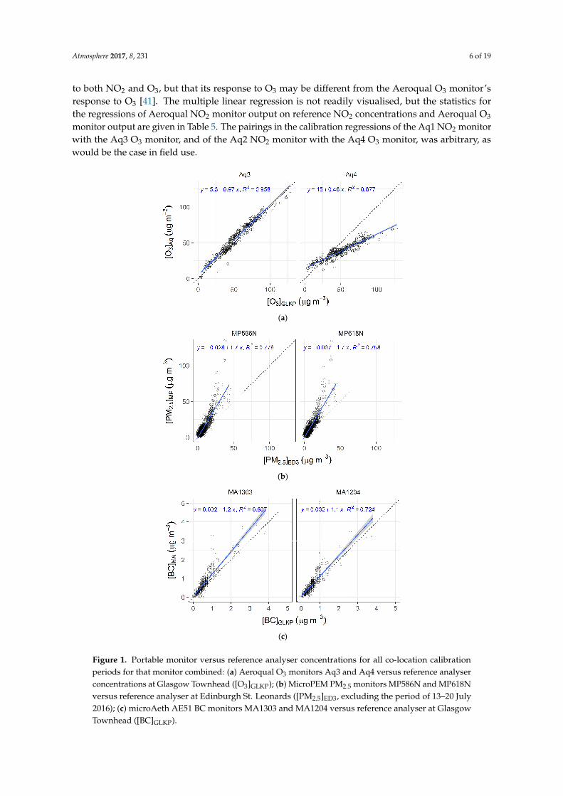
Figure 1 shows the results of regressions for the Aeroqual O3 monitors, the MicroPEM

PM2.5 monitors, and the microAeth BC monitors (two of each) against their respective reference

analyser concentrations for all of their calibration co-location periods combined (‘global’ calibration).

The equivalent plots for each co-location period separately for the O3, PM2.5, and BC monitors are

shown in SI Figures S2–S4, respectively (‘local’ calibrations). The regression statistics are summarised

in Tables 2–4.

The direct comparison plots are not shown for the Aeroqual NO2 monitors because preliminary

investigations of their outputs revealed a clear sensitivity to O3 concentration, as has been noted

previously [36] and for other manufacturers’ NO2 monitors [20]. Lin et al. [36] used the relationship

between [Aeroqual_NO2 − Reference_NO2] and Aeroqual_O3 to calibrate the Aeroqual NO2 monitor

concentrations. This effectively constrains the relationship between Aeroqual_NO2 and Reference_NO2

to be 1:1 (as may be expected for recent factory-calibration). In this study, we used the following

multiple linear regression of Aeroqual_NO2 on both Reference_NO2 and Aeroqual_O3.

Aeroqual_NO2 = k1 × Reference_NO2 + k2 × Aeroqual_O3 + k3

This regression is based on the reasonable expectations that the Aeroqual O3 monitor has a linear

response to ‘true’, i.e., reference analyser, O3, and that the Aeroqual NO2 monitor has a linear response

Atmosphere 2017, 8, 231 6 of 19

to both NO2 and O3, but that its response to O3 may be different from the Aeroqual O3 monitor’s

response to O3 [41]. The multiple linear regression is not readily visualised, but the statistics for

the regressions of Aeroqual NO2 monitor output on reference NO2 concentrations and Aeroqual O3

monitor output are given in Table 5. The pairings in the calibration regressions of the Aq1 NO2 monitor

with the Aq3 O3 monitor, and of the Aq2 NO2 monitor with the Aq4 O3 monitor, was arbitrary, as

would be the case in field use.

(a)

(b)

(c)

Figure 1. Portable monitor versus reference analyser concentrations for all co-location calibration

periods for that monitor combined: (a) Aeroqual O3 monitors Aq3 and Aq4 versus reference analyser

concentrations at Glasgow Townhead ([O3]GLKP); (b) MicroPEM PM2.5 monitors MP586N and MP618N

versus reference analyser at Edinburgh St. Leonards ([PM2.5]ED3, excluding the period of 13–20 July

2016); (c) microAeth AE51 BC monitors MA1303 and MA1204 versus reference analyser at Glasgow

Townhead ([BC]GLKP).

Atmosphere 2017, 8, 231 7 of 19

Measurements from both Aeroqual O3 monitors were highly correlated with reference analyser

concentrations for the combined dataset of all the co-location deployments (R2 = 0.96 and 0.88,

Figure 1a). However, monitor Aq3 had better precision, sensitivity, and bias statistics than monitor

Aq4. Whilst monitor Aq3 had almost 1:1 correspondence with reference analyser concentrations,

monitor Aq4 was only half as sensitive as monitor Aq3. The slope coefficients of regressions for Aq3

declined slightly between individual co-location periods, suggesting a small loss in sensitivity (Table 2,

SI Figure S2). No such trend was obvious for Aq4. The poorer regression statistics for both Aeroqual

monitors during 29 April–4 May 2016 appears to result from the very small dataset, which was caused

by a power cut that curtailed measurements. This co-location periods had so few data points that

its inclusion has a negligible impact on the regression statistics for the combined datasets (Table 2).

Monitor Aq4 also had a poorer correlation with reference O3 during the co-location on 1–4 July (Table 2,

SI Figure S2).

Table 2. Regression statistics of Aeroqual O3 monitor concentrations ([O3]Aq3 and [O3]Aq4) against the

reference analyser at the Glasgow Townhead AURN monitoring station ([O3]GLKP) (hourly averages)

for individual co-location periods and for all of the periods combined. Associated scatter plots shown

in Figure 2a and SI Figure S2.

[O3]Aq3~[O3]GLKP [O3]Aq4~[O3]GLKP

Calibration Period n Slope Intercept/µg m−3R

2 Slope Intercept/µg m−3R

2

9–15 February 2016 105 1.13 3.31 0.973 0.47 14.63 0.90331 March–4 April 2016 97 1.08 2.43 0.963 0.54 10.60 0.88429 April–4 May 2016 6 1.22 −5.41 0.905 0.72 −3.46 0.560 a

4–9 May 2016 119 0.96 4.98 0.976 0.47 16.32 0.88827–31 May 2016 35 0.92 1.57 0.992 0.49 5.94 0.980

1–4 July 2016 67 0.86 5.67 0.954 0.38 22.24 0.539All periods combined 429 0.97 5.33 0.958 0.48 b 14.59 b 0.877 b

a R2 value not significant (p > 0.05). All other R2 values significant; b The exclusion of co-location periods 29 April–4May and 1–4 July changes regression statistics only slightly to slope = 0.49, intercept = 12.90 µg m−3 and R2 = 0.903(n = 362).

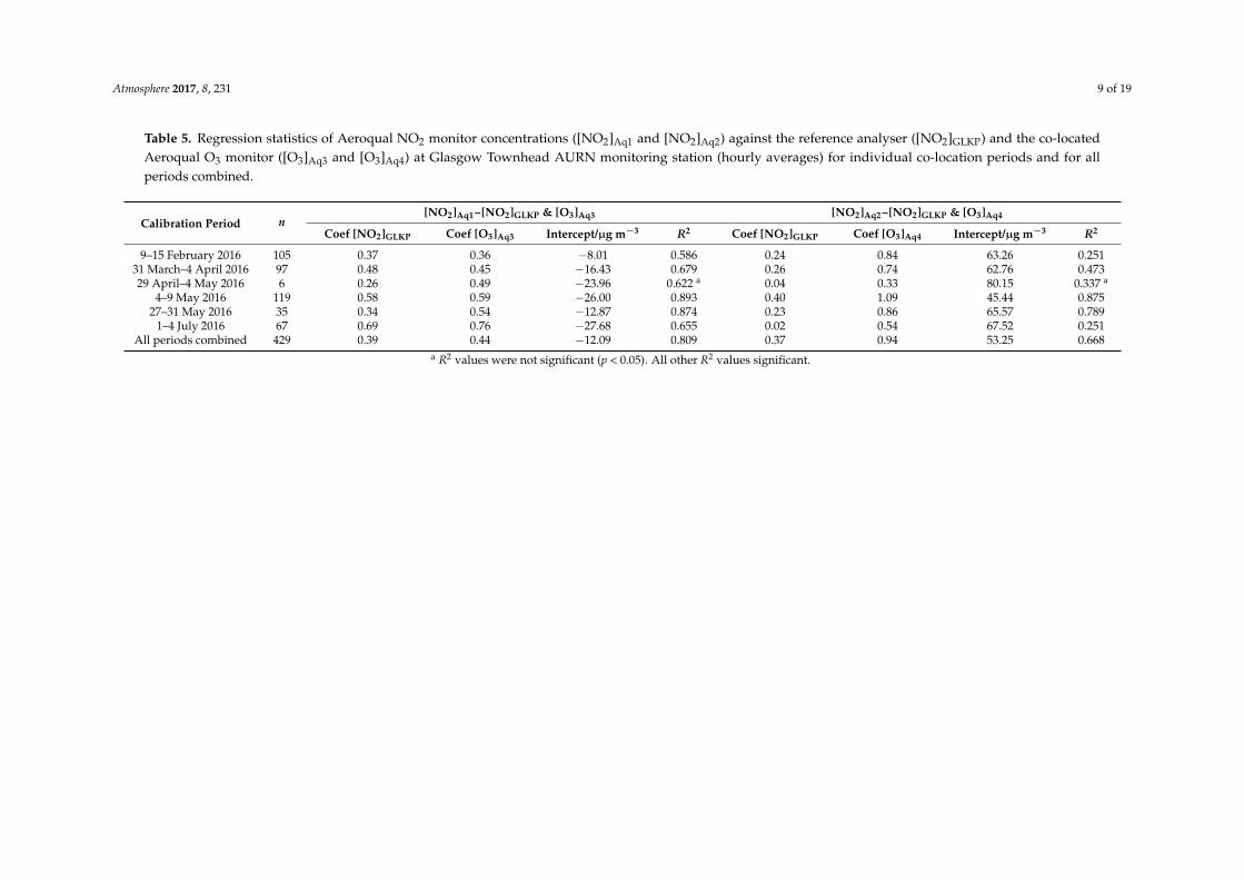
The multiple regressions for the Aeroqual NO2 monitors showed a moderate to high correlation

for the majority of co-deployment periods (R2 = 0.47–0.89, Table 5). Exceptions were for 29 April to

5 May, as noted above for the Aeroqual O3 monitors, when there were only six data points because of

a power cut, and for two other periods for the Aq2 and Aq4 pairing, where R2 = 0.25 (in both cases).

The ‘one off’ poor calibration periods demonstrate the risk of relying on isolated periods of co-location

calibration. The co-location period with only six data points was not used for subsequent calibration;

for mobile measurements around that time the calibration from the next nearest co-deployment

period was used as the local calibration. The data in Table 5 also show that the two sets of Aeroqual

NO2 and O3 monitor pairings had substantially different coefficients in their regression relationships

(particularly the intercepts). This reflects the varying sensitivities of the individual Aeroqual monitors

to their target gas, and, for the NO2 monitors, also to O3.

MicroPEM measurements were also well correlated with TEOM-FDMS reference analyser

concentrations for all of the co-deployment periods combined (R2 = 0.72 and 0.70 for MP586N

and MP618N, respectively, Table 3). SI Figure S3 illustrates generally high correlations between

microPEM monitors and reference analyser for individual co-deployments, except for the period

13–20 July 2016. This one-off poor calibration period again highlights the risk of relying on isolated

periods of co-location calibration. When this period was excluded from the combined dataset of all

the co-deployment periods, the correlation between MicroPEM monitor and analyser increased to

R2 = 0.78 and 0.76 for MP586N and MP618N, respectively) (Figure 1b, Table 3). The regression slopes

indicated that the MicroPEM monitors frequently overestimated when compared with the reference

analyser (Figure 1b). Figure 1b also indicates some non-linearity at PM2.5 concentrations resulting from

greater overestimation of concentrations by the MicroPEM at reference concentrations >~20 µg m−3.

Atmosphere 2017, 8, 231 8 of 19

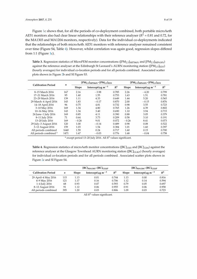
Figure 1c shows that, for all the periods of co-deployment combined, both portable microAeth

AE51 monitors also had clear linear relationships with their reference analyser (R2 = 0.81 and 0.72, for

the MA1303 and MA1204 monitors, respectively). Data for the individual co-deployments indicated

that the relationships of both microAeth AE51 monitors with reference analyser remained consistent

over time (Figure S4, Table 4). However, whilst correlation was again good, regression slopes differed

from 1:1 (Figure 1c).

Table 3. Regression statistics of MicroPEM monitor concentrations ([PM2.5]MP586N and [PM2.5]MP618N)

against the reference analyser at the Edinburgh St Leonard’s AURN monitoring station ([PM2.5]ED3)

(hourly averages) for individual co-location periods and for all periods combined. Associated scatter

plots shown in Figure 2b and SI Figure S3.

Calibration Period n[PM2.5]MP586N~[PM2.5]ED3 [PM2.5]MP618N~[PM2.5]ED3

Slope Intercept/µg m−3R

2 Slope Intercept/µg m−3R

2

8–15 March 2016 167 2.16 −3.98 0.785 2.26 −4.20 0.79917–21 March 2016 95 1.40 1.55 0.753 1.63 1.51 0.78123–29 March 2016 139 1.11 4.33 0.649 1.44 5.20 0.565

29 March–4 April 2016 143 1.83 −0.17 0.870 2.00 −0.15 0.87614–18 April 2016 96 0.75 4.81 0.732 0.98 3.55 0.7233–10 May 2016 169 1.34 4.80 0.765 1.26 4.39 0.80210–16 May 2016 143 1.34 3.40 0.690 1.10 3.94 0.715

24 June–1 July 2016 169 0.85 4.11 0.390 0.88 3.05 0.3798–11 July 2016 71 0.64 3.73 0.209 0.58 3.10 0.19113–20 July 2016 169 −0.26 9.01 0.072 −0.26 8.41 0.073

29 July–3 August 2016 120 1.00 −0.14 0.489 0.98 0.08 0.5223–12 August 2016 159 1.03 1.54 0.384 1.01 1.60 0.397

All periods combined 1640 1.59 0.24 0.717 1.60 0.15 0.700All periods combined a 1471 1.67 −0.03 0.776 1.68 −0.04 0.758

a except period 13–20 July 2016. All R2 values significant.

Table 4. Regression statistics of microAeth monitor concentrations ([BC]1303 and [BC]1204) against the

reference analyser at the Glasgow Townhead AURN monitoring station ([BC]GLKP) (hourly averages)

for individual co-location periods and for all periods combined. Associated scatter plots shown in

Figure 2c and SI Figure S4.

[BC]MA1303~[BC]GLKP [BC]MA1204~[BC]GLKP

Calibration Period n Slope Intercept/µg m−3R

2 Slope Intercept/µg m−3R

2

29 April–4 May 2016 115 1.13 0.01 0.744 1.13 0.00 0.8164–9 May 2016 121 1.17 0.16 0.706 1.12 0.14 0.5941–4 July 2016 68 0.93 0.07 0.593 0.79 0.05 0.697

8–12 August 2016 91 1.12 0.06 0.955 0.91 0.06 0.958All periods combined 395 1.20 0.03 0.806 1.09 0.03 0.723

All R2 values significant.

Atmosphere 2017, 8, 231 9 of 19

Table 5. Regression statistics of Aeroqual NO2 monitor concentrations ([NO2]Aq1 and [NO2]Aq2) against the reference analyser ([NO2]GLKP) and the co-located

Aeroqual O3 monitor ([O3]Aq3 and [O3]Aq4) at Glasgow Townhead AURN monitoring station (hourly averages) for individual co-location periods and for all

periods combined.

Calibration Period n[NO2]Aq1~[NO2]GLKP & [O3]Aq3 [NO2]Aq2~[NO2]GLKP & [O3]Aq4

Coef [NO2]GLKP Coef [O3]Aq3 Intercept/µg m−3R

2 Coef [NO2]GLKP Coef [O3]Aq4 Intercept/µg m−3R

2

9–15 February 2016 105 0.37 0.36 −8.01 0.586 0.24 0.84 63.26 0.25131 March–4 April 2016 97 0.48 0.45 −16.43 0.679 0.26 0.74 62.76 0.47329 April–4 May 2016 6 0.26 0.49 −23.96 0.622 a 0.04 0.33 80.15 0.337 a

4–9 May 2016 119 0.58 0.59 −26.00 0.893 0.40 1.09 45.44 0.87527–31 May 2016 35 0.34 0.54 −12.87 0.874 0.23 0.86 65.57 0.789

1–4 July 2016 67 0.69 0.76 −27.68 0.655 0.02 0.54 67.52 0.251All periods combined 429 0.39 0.44 −12.09 0.809 0.37 0.94 53.25 0.668

a R2 values were not significant (p < 0.05). All other R2 values significant.

Atmosphere 2017, 8, 231 10 of 19

3.2. Evaluation of Portable Monitors during Transient Deployment

As described above, some mobile measurement routes passed by the reference analyser

monitoring station. Reference analyser concentrations are hourly averages and transient co-location

was often of shorter duration. Therefore, to increase the number of comparison data points,

comparisons were included if the transient portable monitor co-location was for 15 min or more

of the hour of the AURN hourly-average value, i.e., a ‘data capture rate’ of ≥25% for each pairwise

comparison. Even with this relaxation in data capture, acquiring a dataset of these transient

comparisons during mobile deployments takes time and effort.

Figure 2a–d show the results of the transient deployment comparisons for the Aeroqual Aq4

O3 and Aq2 NO2 monitors, the MicroPEM MP618N PM2.5 monitor, and the microAeth MA1204 BC

monitor that were used for mobile measurements. The data associated with each transient comparison

are given in Tables S2–S5, respectively. The extent of data capture in each pairwise comparison is

given by the n value in the second column of these tables, which indicates the number of 1-min

portable monitor measurements out of the possible 60 for the full hour for which the reference analyser

value corresponds.

Figure 2a demonstrates the generally closer agreement between monitor estimates and reference

analyser measurements using the global calibration approach when compared to the local calibration

approach for the Aeroqual Aq4 O3 monitor across the whole set of evaluations. Of the 27 periods of

transient standing by the reference analyser monitoring station, the 1-h O3 reference measurement fell

within the interquartile ranges (IQRs) of 17 global linear corrected Aq4 measurements (a proportion

of 63.0%) when compared with seven local linear corrected values (25.9%) and only one uncorrected

measurement (3.7%) (Table S2). The IQR is used here as a simple approximation of a significant

confidence interval; thus, if the reference value falls within the IQR of the corrected monitor value there

is deemed to be no evidence of a significant difference between calibrated monitor value and the test

reference value. If a 50% (rather than 25%) data capture rate (n ≥ 30) was imposed for the co-location

comparison, the advantage of the global linear correction (12 out of 15 co-located periods, 80%) over

the local linear correction (4 out of 15 co-locations, 26.7%) and the uncorrected raw measurements

(none of 15 co-locations, 0%) was clearer (Table S2).

As noted above, the Aeroqual NO2 monitors were subject to interference from O3, and although

this was included in the calibration regression, the relationship between calibrated Aeroqual NO2

estimates and NO2 reference analyser observations deviated more substantially from the 1:1 line than

for the corresponding relationships for the other monitors, and had a lower correlation coefficient than

the O3 and BC monitors (Figure 2). An important consideration is that uncertainty in calibrated

Aeroqual NO2 estimates incorporates the uncertainties in measuring two pollutants. The local

calibration approach for the Aq2 NO2 monitor yielded such extremely scattered corrected data

(Table S3) that it was not appropriate to pursue investigation of this approach, so only data for the global

calibration approach for the Aq2 NO2 monitor are shown in Figure 2b. The figure demonstrates that

the global calibration has substantially improved the Aq2 NO2 monitor agreement with the reference

analyser compared to uncorrected data. Without correction, none of the 27 periods of transient

standing by the reference analyser monitoring station had 1-h NO2 reference measurement within the

interquartile ranges (IQRs) of the Aq2 measurements (Table S3). For the global calibration approach,

the 1-h NO2 reference analyser measurement lay within the IQR of the Aq2 monitor estimates for 21 of

the 27 (i.e., 77.8%) periods (Table S3). However the 1-min Aq2 NO2 estimates, even after adjustment,

were extremely variable, so that the IQRs of the Aq2 NO2 values were wide. The variability extended

to some negative calibrated NO2 estimates which were clearly unrealistic.

The uncorrected and corrected measurements that were made by the MicroPEM MP618N PM2.5

monitor for the transient periods standing adjacent to the monitoring station are shown in Figure 2c.

Neither of the calibration approaches gave closer agreement between calibrated estimates and reference

analyser concentrations than the uncorrected monitor measurement. The 1-h reference measurement

Atmosphere 2017, 8, 231 11 of 19

fell within 2 out of 32 IQRs (6.3%) of the corrected values (for both global and local approaches), when

compared with 6 out of 32 (18.8%) for the uncorrected measurements (SI Table S4).

For the microAeth MA1204 BC monitor used in mobile measurements, Figure 2d shows that the

global calibration approach yields data that corresponds more closely to analyser concentrations as

compared to estimates from the local calibration approach. Out of a total 27 co-located periods, the 1-h

BC reference measurement fell within the IQRs of 16 uncorrected MA1204 measurements (59.3%), but

the global calibration approach increased this to 22 out of 27 of the periods (81.5%). When a 50% data

capture for the comparison was imposed, the global calibration approach reference measurement fell

within the IQRs of 14 out of 17 uncorrected MA1204 measurements (82.4%), as compared with the

local approach (10 out of 17, 58.8%) and no correction (8 out of 17, 47.1%).

(a) (b)

(c) (d)

ΐ ƺ

Figure 2. Portable monitor measurements collected during transient portable deployments standing by

the AURN Glasgow Townhead reference analyser station for (a) the Aeroqual Aq4 O3 monitor; (b) the

Aeroqual Aq2 NO2 monitor; (c) the MicroPEM MP618N PM2.5 monitor, and (d) the microAeth AE51

MA1204 BC monitor. In all of the cases, concentration units are µg m−3, the reference measurements

are the ratified hourly averaged values, and the monitor measurements are the means of 1-min

measurements within the corresponding reference analyser hour. In the majority of cases the transient

co-location was shorter than 1 h, but always greater than 15 min; data in Tables S2–S5 indicate the

duration of each separate co-location for the O3, NO2, PM2.5, and BC portable monitor transient data

collections, respectively. The outer pair of dashed lines in each panel demarcate, respectively, ±30%,

±25%, ±50%, and ±50% from the 1:1 line as guides to expectations of ‘indicative’ measurements for

O3, NO2, PM2.5, and BC (see text for further details).

Atmosphere 2017, 8, 231 12 of 19

4. Discussion

The aim of this work was to develop field-calibration procedures for four types of commercially-

available portable air quality monitors during typical use in exposure assessment research. These

monitors were used over a period of several months that involved repeated cycles of: static co-location

adjacent to reference analysers; use for mobile (walking) measurements; and, intervening periods of

no usage (power off). This experimental design permitted monitor-reference analyser comparisons

for separate co-location periods (‘local’ calibration) and for all of the co-location periods combined

(‘global’ calibration). An additional feature of this study was transient (≤1 h) comparisons of the

portable monitors that were adjacent to the fixed-site reference analysers during mobile deployments.

Although none of the four monitor types used in this study yielded data immediately comparable

to their respective reference analyser during fixed-site co-locations, the generally high correlations

between monitor and reference analyser for the Aeroqual O3, MicroPEM PM2.5 and microAeth BC

monitors (Figure 1 and SI Figures S2–S4), indicated that calibration was feasible. Correlations between

monitor and reference analyser did, however, vary and were not significant for a small number of

co-location periods with reduced concentration ranges (Tables 2–4, and SI Figures S2–S4). There were

no long-term temporal trends in regression coefficients over the multiple co-location deployments

except for a decline in sensitivity of the Aq3 O3 monitor (Tables 2–4, and SI Figures S2–S4). Collectively,

these issues illustrate the strong potential for a single co-location period to yield monitor vs reference

analyser comparison data unrepresentative of the relationship on average. This point is further

illustrated in SI Figures S5–S7, which show scatter plots of the O3, PM2.5, and BC portable monitor

measurements on each mobile deployment day corrected using either the global or local calibration

approaches. The globally or locally calibrated mobile measurements were always well correlated but

were quantitatively different on a number of the days.

The Aeroqual NO2 monitors appeared to be systematically sensitive to O3 since a moderate

correlation between Aeroqual NO2 and reference NO2 could be obtained for the majority of

co-deployments by inclusion of Aeroqual O3 values in a multiple linear regression (Table 5).

A sensitivity of the Aeroqual electrochemical NO2 sensor to O3 in field deployments has been noted

before [36,41]. Correction for this cross-sensitivity is therefore feasible in principle by using an Aeroqual

O3 sensor in tandem with the Aeroqual NO2 sensor; however, the application of a correction function

involving output from another monitor adds the uncertainty that is intrinsic to the second monitor to

the uncertainty already intrinsic to the first monitor. The inherent variability in the regression resulted

in instances of negative calibrated NO2 concentration estimates when the calibration regression was

applied to separate measurements that were made during mobile deployment (Figure 2b, Table S3).

The advantage of merging all the periods of co-location into one ‘global’ calibration dataset

was further demonstrated by the experiments to independently evaluate the monitor calibrations

during mobile usage on different days to those that were used to establish calibration relationships

(Figure 2). The improved comparison statistics for the global calibration approach was particularly

evident for the Aeroqual O3 and microAeth BC monitors. Since the regression relationship in any

individual co-location period sometimes differed from the overall average regression (for identifiable

or not-identifiable reasons), the global calibration approach is recommended. These global calibrations

should be derived from several individual co-location periods bounding the time period of the field

measurements. It is acknowledged, however, that due to possible longer-term changes in instrument

response, a given calibration should not be extrapolated over time periods longer than a few months.

The generally poorer agreement between calibrated MicroPEM monitor estimates and

TEOM-FDMS measurements (when compared with other monitors that are evaluated here) in the

independent evaluation during mobile usage, irrespective of correction, may be attributable to the

greater uncertainty in measurements of the low ambient concentrations of PM2.5 when compared with

e.g., O3. The ambient PM2.5 concentrations encountered throughout this study were generally low, even

in central Glasgow, and both the reference analyser and the MicroPEM monitors have acknowledged

the limitations in measuring PM2.5 concentrations of just a few µg m−3 [42,43]. Furthermore, the

Atmosphere 2017, 8, 231 13 of 19

smaller concentration range often recorded for ambient PM2.5 than for NO2 and O3 limits the extent

of variation that can be explained by calibration and evaluation statistics. Since the calibration of

the MicroPEM MP618 monitor was derived at the Edinburgh St. Leonard’s reference site (ED3), but

was evaluated at the Glasgow Townhead referenced site (GLKP), this may also highlight a limitation

of extrapolation from fixed-site calibrations. Finally, it is noted again that the MicroPEM monitor

does not directly measure PM2.5 mass but uses an internal factor based on assumptions about the

size distribution and optical properties of the sampled particles to convert scattered light into a PM2.5

value. This introduces unquantifiable uncertainty into the MicroPEM measurements if the size and

optical properties of the actual particle mix differ from that on which the internal factor is based.

Our findings for portable monitor performance against their respective analyser are compared

here with some relevant previous literature. Delgado-Saborit [15] reported similar slope and intercept

(y = 0.9727x + 0.0938, R2 = 0.8937) between a microAeth AE51 and an Aethalometer AE41 analyser

from a four-day co-location study in Birmingham. The Aeroqual NO2 monitor co-located with a

Horiba APNA370 NOx chemiluminescence analyser for seven days showed a better agreement than

in this study (y = 0.7569x + 7.0505, R2 = 0.6321). A co-location of four AE51 BC monitors alongside

the reference AE22 under lab conditions in Shanghai found an averaged slope of 1.04 and an average

intercept of −0.09 (R2 = 0.960) between twelve 24-h averaged BC concentration measurements [44]; both

are similar to our study (slope = 0.79–1.13, intercept = 0.00–0.14, R2 = 0.594–0.958). A co-location of

Aeroqual O3 monitors alongside reference analysers in and around the City of Arvin, California,

recorded slopes of 1.001–1.051 and intercepts of −3.28–−0.015 ppb (R2 = 0.926–0.984) between

measurements made by the two techniques [45]. While the comparison between our Aeroqual Aq4

monitor and its reference analyser always had slope less than 1 (0.38–0.72) and a more varying

intercept (−3.46–22.24 µg m−3), the Aq3-Ref-analyser pairing had parameters similar to this US

study (slope = 0.86–1.22, intercept = −5.41–5.67 µg m−3, R2 = 0.905–0.992). This was also similar to a

previous study of a different Aeroqual O3 monitor in Edinburgh, UK, over five weeks in summer where

a slope of 1.16 and an intercept of −6.82 µg m−3 (R2 = 0.91) were observed [36]. Finally, Sloan et al. [43]

reported significant difference (difference = 2.2 µg m−3, p < 0.0001) between measurements of PM2.5

by MicroPEM and the reference analyser over ~5 h co-location at Lindon air quality monitoring station

in Utah County, US. However, this was for 5 h only and no slope or intercept was reported.

It is important to consider the extent to which calibrated observations during measurement

periods are, or are not, extrapolated outside of the range of sensor responses that occurred during

calibration periods. The extent of extrapolation during transient co-locations can be assessed by

comparing the axis scales on the scatter plots in Figures 1 and 2. For O3 and BC, the ranges of measured

concentrations by both reference and portable monitors are of similar magnitude during calibration

and measurement periods (as one would hope for); with the range of measurements made during the

calibration periods encompassing the range of measurements during the transient co-location periods.

Approximately 66% and 42% of the calibration ranges were represented by transient co-location ranges

for O3 and BC. For PM2.5, the range of the majority of measurements during the transient co-location

periods is about 22% of the range of PM2.5 measurements during the calibration periods. Thus, there is

no extrapolation outside of the range of calibration measurements. Nevertheless, this discrepancy is a

reminder that the relatively large range of PM2.5 measurements during calibration periods probably

results from higher concentrations that were observed during periods of long-range transport of

particles [46]. These relatively large changes in PM2.5 concentrations originating from distant sources

may, or may not (e.g., through different optical properties of aged accumulation mode particles vs.

recently emitted/re-suspended particles), accurately represent the relatively small temporal changes

in PM2.5 in our transient co-locations, and the increments between background and roadside locations

that we attempt to quantify in subsequent mobile measurements. However, without detailed chemical,

size, and/or optical measurements of the PM2.5, is not possible to know the extent to which calibration

may be impacted, but this is the case with any measurements that are made using these types of

portable PM instruments. The interpretation of ranges during calibration, transient co-location, and

Atmosphere 2017, 8, 231 14 of 19

mobile measurement for NO2 measured by Aeroqual sensors is complicated through the requirement

for a multivariate calibration approach to allow for apparent dual sensitivity of the Aeroqual NO2

sensors to both NO2 and O3. The presence of negative adjusted Aeroqual NO2 concentrations during

transient co-locations (Figure 2b) may indicate that calibrated Aeroqual estimates were affected by

extrapolation beyond the measured ranges during calibration. The presence of negative values is

discussed further below.

Collectively, the above considerations give greater confidence in the reliability of ‘globally’

calibrated estimates from the O3 and BC portable instruments for characterisation of temporal and

spatial concentration variations when compared to the reliability of ‘globally’ calibrated estimates from

the PM2.5 and NO2 portable instruments, as a result of the differences in measurement concentration

ranges cf. calibration concentration ranges for the latter two pollutant metrics. The limited range of

concentrations during ‘local’ calibration periods is the likely cause of differences between ‘globally’

and ‘locally’ calibrated estimates.

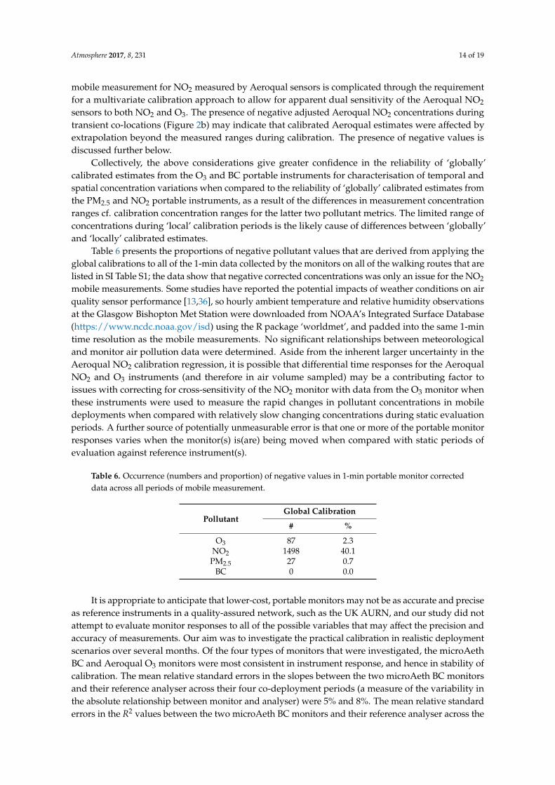
Table 6 presents the proportions of negative pollutant values that are derived from applying the

global calibrations to all of the 1-min data collected by the monitors on all of the walking routes that are

listed in SI Table S1; the data show that negative corrected concentrations was only an issue for the NO2

mobile measurements. Some studies have reported the potential impacts of weather conditions on air

quality sensor performance [13,36], so hourly ambient temperature and relative humidity observations

at the Glasgow Bishopton Met Station were downloaded from NOAA’s Integrated Surface Database

(https://www.ncdc.noaa.gov/isd) using the R package ‘worldmet’, and padded into the same 1-min

time resolution as the mobile measurements. No significant relationships between meteorological

and monitor air pollution data were determined. Aside from the inherent larger uncertainty in the

Aeroqual NO2 calibration regression, it is possible that differential time responses for the Aeroqual

NO2 and O3 instruments (and therefore in air volume sampled) may be a contributing factor to

issues with correcting for cross-sensitivity of the NO2 monitor with data from the O3 monitor when

these instruments were used to measure the rapid changes in pollutant concentrations in mobile

deployments when compared with relatively slow changing concentrations during static evaluation

periods. A further source of potentially unmeasurable error is that one or more of the portable monitor

responses varies when the monitor(s) is(are) being moved when compared with static periods of

evaluation against reference instrument(s).

Table 6. Occurrence (numbers and proportion) of negative values in 1-min portable monitor corrected

data across all periods of mobile measurement.

PollutantGlobal Calibration

# %

O3 87 2.3NO2 1498 40.1

PM2.5 27 0.7BC 0 0.0

It is appropriate to anticipate that lower-cost, portable monitors may not be as accurate and precise

as reference instruments in a quality-assured network, such as the UK AURN, and our study did not

attempt to evaluate monitor responses to all of the possible variables that may affect the precision and

accuracy of measurements. Our aim was to investigate the practical calibration in realistic deployment

scenarios over several months. Of the four types of monitors that were investigated, the microAeth

BC and Aeroqual O3 monitors were most consistent in instrument response, and hence in stability of

calibration. The mean relative standard errors in the slopes between the two microAeth BC monitors

and their reference analyser across their four co-deployment periods (a measure of the variability in

the absolute relationship between monitor and analyser) were 5% and 8%. The mean relative standard

errors in the R2 values between the two microAeth BC monitors and their reference analyser across the

Atmosphere 2017, 8, 231 15 of 19

co-deployment periods (a measure of the variability in the precision) were 10% and 10%. For the two

Aeroqual O3 monitors the corresponding mean relative standard errors in monitor-reference slope

were 5% and 10%, and mean relative standard errors in monitor-reference R2 values were 1% and

10%. Reproducibility in a quantitative calibration relationship for the MicroPEM PM2.5 monitors was

poorer than for the BC and O3 monitors (mean relative standard errors in slope for the two MicroPEM

instruments were 16% and 16%), which, as discussed above, is potentially attributable to the low

values and ranges of ambient PM2.5 concentrations. Nevertheless, the generally high correlations

with temporal changes in PM2.5, as measured by the reference analyser (Table 3) gives confidence in

the relative trends of PM2.5 data from these monitors (i.e., lower vs. higher pollutant concentration

between locations and/or between two points), for the time averaging of 1 h used here. Indeed,

the calibrations of all the O3, BC, and PM2.5 monitors, derived from a single dataset of periods of

field co-location against their respective reference analysers, appears sufficient to yield ‘indicative’

quantitative concentrations. In European Union (EU) air quality legislation an ‘indicative’ method is

where the relative expanded uncertainty of a measurement is within 30% for O3, 25% for NO2, and

50% for PM2.5 at their respective limit or target value [47]. These uncertainty ranges are marked on

Figure 2 (the uncertainty tolerance for PM2.5 is used for the BC data in Figure 2d). In all instances, the

‘globally’ calibrated BC monitor measurements from the independent ‘transient’ calibration periods

lie within the tolerance for an ‘indicative’ measurement (Figure 2d), and in the majority of cases the

O3 and PM2.5 monitor calibrated values are also in their respective indicative ranges (Figure 2a,c).

The performance of the Aeroqual O3 and MicroPEM monitors was also reported favourably in the

AQ-SPEC program (www.aqmd.gov/aq-spec/evaluations/summary).

Despite this generally satisfactory demonstration of ‘indicative’ measurement for the O3, BC, and

PM2.5 monitors, it is emphasised that this should not be over-interpreted. We have presented only data

from a single study, albeit over an extended time period. For the O3 and BC monitors, we compared

calibrated monitor output at the same site where we derived global calibration relationships, albeit

for different times. In most instances, the measurements that were made during mobile usage for the

transient checks on calibration were for less than the full hour of a reference analyser measurement and

were slightly further from the reference analyser inlet than for the static co-deployments. On the other

hand, our study has sought to evaluate monitor calibration during actual mobile deployments of these

monitors, which previous studies have not. Acquiring a dataset of these transient comparisons during

mobile deployments takes time and effort—e.g., standing with a portable monitor by a reference

monitoring station for an hour yields only a single data comparison pair. It also needs to be noted that

the reference analyser data, even with formal QA/QC and data ratification processes, are only required

to satisfy expanded absolute uncertainties within ±15% for O3 and NO2 and 25% for PM2.5 [47].

5. Conclusions

We have shown that with the implementation of repeated field calibration cycles, it is possible to

attain indicative measurement accuracy for the Aeroqual O3, microAeth BC, and MicroPEM PM2.5

portable monitors used in this study. For studies of a few months duration, it is recommended to

use a ‘global’ calibration that is derived from a set of co-locations with a reference analyser rather

than calibrations from a single co-location deployment nearest in time to a given mobile deployment

period. However, it is important to emphasise that although the capital and consumable costs of the

portable monitors used here were much lower than for the reference analysers, it was necessary to

devote substantial time and effort to calibrate and post-process the portable measurements to attain

this outcome. Our study also only considered portable monitor application outdoors, not personal

exposures switching between outdoor, in-transit, and indoor environments. The Aeroqual NO2

monitors that were used in this study had interference from O3; and whilst work presented here and

elsewhere suggests the potential for reasonably-effective correction using O3 measurements in tandem

with the NO2 measurements during extended periods of fixed-site deployment, the correction here did

not extrapolate consistently to calibration of NO2 measurements during mobile deployments, for the

Atmosphere 2017, 8, 231 16 of 19

possible reasons discussed above. However, with the continued development in sensor technology, it

may be anticipated that sensor-based portable monitors will increasingly provide additional relevant

information to existing air quality monitoring.

Supplementary Materials: Supplementary information referred to in the paper is available online at www.mdpi.com/2073-4433/8/12/231/s1.

Acknowledgments: This work was jointly funded under Natural Environment Research Council (NERC) grantNE/N007352/1 and Innovate UK project 102354. Co-author N.M. also acknowledges funding from NERC CASEPhD studentship NE/K007319/1, with support from Ricardo Energy and Environment, and co-author H.W.acknowledges funding from the University of Edinburgh and the NERC Centre for Ecology & Hydrology (NERCCEH project number NEC04544). Brian Shaw and Nuoxi Zhang (University of Edinburgh) assisted with some ofthe mobile measurements. The AURN measurement data were obtained from uk-air.defra.gov.uk and are subjectto Crown 2014 copyright, Defra, licensed under the Open Government Licence (OGL).

Author Contributions: David J. Carruthers, Mark Jackson, Ruth M. Doherty, Mathew R. Heal and Iain J. Beverlandconceived the work and its broad methodology; Stefan Reis provided additional instrumentation. Chun Lin,Mathew R. Heal and Iain J. Beverland devised the detailed experimental methodology with additional inputfrom all authors. Chun Lin, Nicola Masey and Hao Wu undertook measurements. Chun Lin with input fromMathew R. Heal, Iain J. Beverland, Nicola Masey and Hao Wu undertook data presentation and analysis. Chun Linand Mathew R. Heal wrote the first draft of the manuscript; all authors reviewed and contributed edits to finalisethe manuscript.

Conflicts of Interest: The authors declare no conflicts of interest.

References

1. WHO. Air Quality Guidelines Global Update 2005. In Particulate Matter, Ozone, Nitrogen Dioxide and

Sulfur Dioxide; World Health Organisation Regional Office for Europe: Copenhagen, Denmark, 2006;

ISBN 92 890 2192 6. Available online: http://www.euro.who.int/__data/assets/pdf_file/0005/78638/

E90038.pdf (accessed on 20 October 2017).

2. WHO. Review of Evidence on Health Aspects of Air Pollution—REVIHAAP Project; Technical Report;

World Health Organisation: Copenhagen, Denmark, 2013; Available online: http://www.euro.who.int/

__data/assets/pdf_file/0004/193108/REVIHAAP-Final-technical-report-final-version.pdf (accessed on

20 October 2017).

3. WHO. Health Risks of Air Pollution in Europe—HRAPIE Project; World Health Organisation: Copenhagen,

Denmark, 2013; Available online: http://www.euro.who.int/en/health-topics/environment-and-health/

air-quality/publications/2013/health-risks-of-air-pollution-in-europe-hrapie-project-recommendations-

for-concentrationresponse-functions-for-costbenefit-analysis-of-particulate-matter,-ozone-and-nitrogen-

dioxide (accessed on 20 October 2017).

4. WHO. Health Effects of Black Carbon; World Health Organisation Regional Office for Europe: Copenhagen,

Denmark, 2012; ISBN 978 92 890 0265 3. Available online: http://www.euro.who.int/__data/assets/pdf_

file/0004/162535/e96541.pdf (accessed on 20 October 2017).

5. Grahame, T.J.; Klemm, R.; Schlesinger, R.B. Public health and components of particulate matter: The changing

assessment of black carbon. J. Air Waste Manag. Assoc. 2014, 64, 620–660. [CrossRef] [PubMed]

6. Snyder, E.G.; Watkins, T.H.; Solomon, P.A.; Thoma, E.D.; Williams, R.W.; Hagler, G.S.W.; Shelow, D.;

Hindin, D.A.; Kilaru, V.J.; Preuss, P.W. The Changing Paradigm of Air Pollution Monitoring. Environ. Sci.

Technol. 2013, 47, 11369–11377. [CrossRef] [PubMed]

7. Steinle, S.; Reis, S.; Sabel, C.E. Quantifying human exposure to air pollution—Moving from static monitoring

to spatio-temporally resolved personal exposure assessment. Sci. Total Environ. 2013, 443, 184–193. [CrossRef]

[PubMed]

8. Kumar, P.; Morawska, L.; Martani, C.; Biskos, G.; Neophytou, M.; Di Sabatino, S.; Bell, M.; Norford, L.;

Britter, R. The rise of low-cost sensing for managing air pollution in cities. Environ. Int. 2015, 75, 199–205.

[CrossRef] [PubMed]

9. Lewis, A.; Edwards, P. Validate personal air-pollution sensors. Nature 2016, 535, 29–31. [CrossRef] [PubMed]

10. McKercher, G.R.; Salmond, J.A.; Vanos, J.K. Characteristics and applications of small, portable gaseous air

pollution monitors. Environ. Pollut. 2017, 223, 102–110. [CrossRef] [PubMed]

Atmosphere 2017, 8, 231 17 of 19

11. Rai, A.C.; Kumar, P.; Pilla, F.; Skouloudis, A.N.; Di Sabatino, S.; Ratti, C.; Yasar, A.; Rickerby, D. End-user

perspective of low-cost sensors for outdoor air pollution monitoring. Sci. Total Environ. 2017, 607, 691–705.

[CrossRef] [PubMed]

12. Mead, M.I.; Popoola, O.A.M.; Stewart, G.B.; Landshoff, P.; Calleja, M.; Hayes, M.; Baldovi, J.J.; McLeod, M.W.;

Hodgson, T.F.K.; Dicks, J.; et al. The use of electrochemical sensors for monitoring urban air quality in

low-cost, high-density networks. Atmos. Environ. 2013, 70, 186–203. [CrossRef]

13. Bart, M.; Williams, D.E.; Ainslie, B.; McKendry, I.; Salmond, J.; Grange, S.K.; Alavi-Shoshtari, M.; Steyn, D.;

Henshaw, G.S. High Density Ozone Monitoring Using Gas Sensitive Semi-Conductor Sensors in the Lower

Fraser Valley, British Columbia. Environ. Sci. Technol. 2014, 48, 3970–3977. [CrossRef] [PubMed]

14. Heimann, I.; Bright, V.B.; McLeod, M.W.; Mead, M.I.; Popoola, O.A.M.; Stewart, G.B.; Jones, R.L. Source

attribution of air pollution by spatial scale separation using high spatial density networks of low cost air

quality sensors. Atmos. Environ. 2015, 113, 10–19. [CrossRef]

15. Delgado-Saborit, J.M. Use of real-time sensors to characterise human exposures to combustion related

pollutants. J. Environ. Monit. 2012, 14, 1824–1837. [CrossRef] [PubMed]

16. Hankey, S.; Marshall, J.D. On-bicycle exposure to particulate air pollution: Particle number, black carbon,

PM2.5, and particle size. Atmos. Environ. 2015, 122, 65–73. [CrossRef]

17. Van den Bossche, J.; Peters, J.; Verwaeren, J.; Botteldooren, D.; Theunis, J.; De Baets, B. Mobile monitoring for

mapping spatial variation in urban air quality: Development and validation of a methodology based on an

extensive dataset. Atmos. Environ. 2015, 105, 148–161. [CrossRef]

18. Deville Cavellin, L.; Weichenthal, S.; Tack, R.; Ragettli, M.S.; Smargiassi, A.; Hatzopoulou, M. Investigating

the Use Of Portable Air Pollution Sensors to Capture the Spatial Variability Of Traffic-Related Air Pollution.

Environ. Sci. Technol. 2016, 50, 313–320. [CrossRef] [PubMed]

19. Gillespie, J.; Masey, N.; Heal, M.R.; Hamilton, S.; Beverland, I.J. Estimation of spatial patterns of urban air

pollution over a 4-week period from repeated 5-min measurements. Atmos. Environ. 2017, 150, 295–302.

[CrossRef]

20. Duvall, R.M.; Long, R.W.; Beaver, M.R.; Kronmiller, K.G.; Wheeler, M.L.; Szykman, J.J. Performance

Evaluation and Community Application of Low-Cost Sensors for Ozone and Nitrogen Dioxide. Sensors 2016,

16, 1698. [CrossRef] [PubMed]

21. Thompson, J.E. Crowd-sourced air quality studies: A review of the literature & portable sensors.

Trends Environ. Anal. Chem. 2016, 11, 23–34.

22. Castell, N.; Dauge, F.R.; Schneider, P.; Vogt, M.; Lerner, U.; Fishbain, B.; Broday, D.; Bartonova, A.

Can commercial low-cost sensor platforms contribute to air quality monitoring and exposure estimates?

Environ. Int. 2017, 99, 293–302. [CrossRef] [PubMed]

23. Jerrett, M.; Donaire-Gonzalez, D.; Popoola, O.; Jones, R.; Cohen, R.C.; Almanza, E.; de Nazelle, A.; Mead, I.;

Carrasco-Turigas, G.; Cole-Hunter, T.; et al. Validating novel air pollution sensors to improve exposure

estimates for epidemiological analyses and citizen science. Environ. Res. 2017, 158, 286–294. [CrossRef]

[PubMed]

24. Spinelle, L.; Gerboles, M.; Aleixandre, M. Performance evaluation of amperometric sensors for the monitoring

of O3 and NO2 in ambient air at ppb level. Procedia Eng. 2015, 120, 480–483. [CrossRef]

25. Lewis, A.C.; Lee, J.D.; Edwards, P.M.; Shaw, M.D.; Evans, M.J.; Moller, S.J.; Smith, K.R.; Buckley, J.W.;

Ellis, M.; Gillot, S.R.; et al. Evaluating the performance of low cost chemical sensors for air pollution research.

Faraday Discuss. 2016, 189, 85–103. [CrossRef] [PubMed]

26. Manikonda, A.; Zikova, N.; Hopke, P.K.; Ferro, A.R. Laboratory assessment of low-cost PM monitors.

J. Aerosol Sci. 2016, 102, 29–40. [CrossRef]

27. Borrego, C.; Costa, A.M.; Ginja, J.; Amorim, M.; Coutinho, M.; Karatzas, K.; Sioumis, T.; Katsifarakis, N.;

Konstantinidis, K.; de Vito, S.; et al. Assessment of air quality microsensors versus reference methods: The

EuNetAir joint exercise. Atmos. Environ. 2016, 147, 246–263. [CrossRef]

28. Wallace, L.A.; Wheeler, A.J.; Kearney, J.; Van Ryswyk, K.; You, H.; Kulka, R.H.; Rasmussen, P.E.; Brook, J.R.;

Xu, X. Validation of continuous particle monitors for personal, indoor, and outdoor exposures. J. Expos. Sci.

Environ. Epidemiol. 2011, 21, 49–64. [CrossRef] [PubMed]

29. Tasic, V.; Jovasevic-Stojanovic, M.; Vardoulakis, S.; Milosevic, N.; Kovacevic, R.; Petrovic, J. Comparative

assessment of a real-time particle monitor against the reference gravimetric method for PM10 and PM2.5 in

indoor air. Atmos. Environ. 2012, 54, 358–364. [CrossRef]

Atmosphere 2017, 8, 231 18 of 19

30. Williams, D.E.; Henshaw, G.S.; Bart, M.; Laing, G.; Wagner, J.; Naisbitt, S.; Salmond, J.A. Validation of

low-cost ozone measurement instruments suitable for use in an air-quality monitoring network. Meas. Sci.

Technol. 2013, 24, 065803. [CrossRef]

31. Steinle, S.; Reis, S.; Sabel, C.E.; Semple, S.; Twigg, M.M.; Braban, C.F.; Leeson, S.R.; Heal, M.R.; Harrison, D.;

Lin, C.; et al. Personal exposure monitoring of PM2.5 in indoor and outdoor microenvironments. Sci. Total

Environ. 2015, 508, 383–394. [CrossRef] [PubMed]

32. Viana, M.; Rivas, I.; Reche, C.; Fonseca, A.S.; Perez, N.; Querol, X.; Alastuey, A.; Alvarez-Pedrerol, M.;

Sunyer, J. Field comparison of portable and stationary instruments for outdoor urban air exposure

assessments. Atmos. Environ. 2015, 123, 220–228. [CrossRef]

33. Williams, R.; Long, R.; Beaver, M.; Kaufman, A.; Zeiger, F.; Heimbinder, M.; Hang, I.; Yap, R.; Acharya, B.;

Ginwald, B.; et al. Sensor Evaluation Report; EPA/600/R-14/143 (NTIS PB2015-100611); United States

Environmental Protection Agency: Washington, DC, USA, 2014. Available online: https://cfpub.epa.gov/

si/si_public_record_report.cfm?dirEntryId=277270 (accessed on 20 October 2017).

34. Williams, R.; Kaufman, A.; Hanley, T.; Rice, J.; Garvey, S. Evaluation of Field—Deployed Low Cost PM Sensors;

EPA/600/R-14/464 (NTIS PB 2015-102104); United States Environmental Protection Agency: Washington,

DC, USA, 2014. Available online: http://cfpub.epa.gov/si/si_public_record_report.cfm?dirEntryId=297517

(accessed on 20 October 2017).

35. Jiao, W.; Hagler, G.; Williams, R.; Sharpe, R.; Brown, R.; Garver, D.; Judge, R.; Caudill, M.; Rickard, J.;

Davis, M.; et al. Community Air Sensor Network (CAIRSENSE) project: Evaluation of low-cost sensor

performance in a suburban environment in the southeastern United States. Atmos. Meas. Technol. 2016, 9,

5281–5292. [CrossRef]

36. Lin, C.; Gillespie, J.; Schuder, M.D.; Duberstein, W.; Beverland, I.J.; Heal, M.R. Evaluation and calibration of

Aeroqual Series 500 portable gas sensors for accurate measurement of ambient ozone and nitrogen dioxide.

Atmos. Environ. 2015, 100, 111–116. [CrossRef]

37. Spinelle, L.; Gerboles, M.; Villani, M.G.; Aleixandre, M.; Bonavitacola, F. Field calibration of a cluster of

low-cost available sensors for air quality monitoring. Part A: Ozone and nitrogen dioxide. Sens. Actuators

B Chem. 2015, 215, 249–257. [CrossRef]

38. Heal, M.R.; Kumar, P.; Harrison, R.M. Particles, air quality, policy and health. Chem. Soc. Rev. 2012, 41,

6606–6630. [CrossRef] [PubMed]

39. Hagler, G.S.W.; Yelverton, T.L.B.; Vedantham, R.; Hansen, A.D.A.; Turner, J.R. Post-processing Method to

Reduce Noise while Preserving High Time Resolution in Aethalometer Real-time Black Carbon Data. Aerosol

Air Qual. Res. 2011, 11, 539–546. [CrossRef]

40. Apte, J.S.; Kirchstetter, T.W.; Reich, A.H.; Deshpande, S.J.; Kaushik, G.; Chel, A.; Marshall, J.D.; Nazaroff, W.W.

Concentrations of fine, ultrafine, and black carbon particles in auto-rickshaws in New Delhi, India.

Atmos. Environ. 2011, 45, 4470–4480. [CrossRef]

41. Masey, N.; Gillespie, J.; Ezani, E.; Lin, C.; Wu, H.; Ferguson, N.S.; Hamilton, S.; Heal, M.R.; Beverland, I.J.

Temporal changes in field calibration relationships for Aeroqual S500 O3 and NO2 sensor-based monitors.

Sens. Actuators B 2017. submitted.

42. Air Quality Expert Group (AQEG). Fine Particulate Matter (PM2.5) in the United Kingdom; PB13837;

Department for Environment, Food and Rural Affairs: London, UK, 2012. Available online: http:

//uk-air.defra.gov.uk/library/reports?report_id=727 (accessed on 20 October 2017).

43. Sloan, C.D.; Philipp, T.J.; Bradshaw, R.K.; Chronister, S.; Barber, W.B.; Johnston, J.D. Applications of

GPS-tracked personal and fixed-location PM2.5 continuous exposure monitoring. J. Air Waste Manag. Assoc.

2016, 66, 53–65. [CrossRef] [PubMed]

44. Cai, J.; Yan, B.Z.; Ross, J.; Zhang, D.N.; Kinney, P.L.; Perzanowski, M.S.; Jung, K.; Miller, R.; Chillrud, S.N.

Validation of MicroAeth (R) as a Black Carbon Monitor for Fixed-Site Measurement and Optimization for

Personal Exposure Characterization. Aerosol Air Qual. Res. 2014, 14, 1–9. [CrossRef] [PubMed]

45. MacDonald, C.P.; Roberts, P.T.; McCarthy, M.C.; DeWinter, J.L.; Dye, T.S.; Vaughn, D.L.; Henshaw, G.;

Nester, S.; Minor, H.A.; Rutter, A.P.; et al. Ozone Concentrations in and Around the City of Arvin, California;

STI-913040-5865-FR2, Final Report Prepared for the San Joaquin Valley Unified Air Pollution Control District,

Fresno, CA; Sonoma Technology Inc.: Petaluma, CA, USA, 2014. Available online: www.valleyair.org/air_

quality_plans/docs/2013attainment/ozonesaturationstudy.pdf (accessed on 20 October 2017).

Atmosphere 2017, 8, 231 19 of 19

46. Buchanan, C.M.; Beverland, I.J.; Heal, M.R. The influence of weather-type and long-range transport on

airborne particle concentrations in Edinburgh, UK. Atmos. Environ. 2002, 36, 5343–5354. [CrossRef]

47. EC. Directive Directive 2008/50/EC of the European Parliament and of the Council of 21 May 2008 on

Ambient Air Quality and Cleaner Air for Europe. 2008. Available online: http://eur-lex.europa.eu/

LexUriServ/LexUriServ.do?uri=CELEX:32008L0050:EN:NOT (accessed on 20 October 2017).

© 2017 by the authors. Licensee MDPI, Basel, Switzerland. This article is an open access

article distributed under the terms and conditions of the Creative Commons Attribution

(CC BY) license (http://creativecommons.org/licenses/by/4.0/).