LIMITATIONS ON INCREASES IN PROPERTY TAX ASSESSED VALUE David L. Sjoquist Lakshmi Pandey

FRP Report No. 37 November 1999

2

ACKNOWLEDGMENTS

This report was prepared with the valuable research assistance of Steve Maguire,

Darmen Zhumadil, and Joey Smith.

iii

TABLE OF CONTENTS

Page

Executive Summary . . . . . . . . . . . . . . . . . . . . . . . . . . . . . . . . . . . . . . . . . . . . . . . . . . . . . . . . . iv

I. Introduction . . . . . . . . . . . . . . . . . . . . . . . . . . . . . . . . . . . . . . . . . . . . . . . . . . . . . . . . . . 1

II. Existing Limitations . . . . . . . . . . . . . . . . . . . . . . . . . . . . . . . . . . . . . . . . . . . . . . . . . . . . 2

III. The Constitutionality of Assessment Increase Limitations . . . . . . . . . . . . . . . . . . . . . . . . 6

IV. Economic Effects of Assessment Increase Limitations . . . . . . . . . . . . . . . . . . . . . . . . . . 7

A. Effect of Assessment Limitations on the Level of Property Taxes . . . . . . . . . . . . . . . 7

B. Distributional Effects of Assessment Limitations . . . . . . . . . . . . . . . . . . . . . . . . . . . . 8

C. Other Economics Effects of Acquisition Value Assessment . . . . . . . . . . . . . . . . . . . 14

V. Property Tax Assessment Limitations in Muscogee County . . . . . . . . . . . . . . . . . . . . . 15

A. The Effect on Aggregate Property Tax Digest . . . . . . . . . . . . . . . . . . . . . . . . . . . . 16

B. An Analysis of Assessment Disparities . . . . . . . . . . . . . . . . . . . . . . . . . . . . . . . . . . 20

C. An Analysis by Socio-Economic Characteristic . . . . . . . . . . . . . . . . . . . . . . . . . . . . 25

D. Mobility . . . . . . . . . . . . . . . . . . . . . . . . . . . . . . . . . . . . . . . . . . . . . . . . . . . . . . . . . 26

VI. Conclusions . . . . . . . . . . . . . . . . . . . . . . . . . . . . . . . . . . . . . . . . . . . . . . . . . . . . . . . . . 29

References . . . . . . . . . . . . . . . . . . . . . . . . . . . . . . . . . . . . . . . . . . . . . . . . . . . . . . . . . . . . . . . . 30

iv

LIMITATIONS ON INCREASES IN PROPERTY TAX ASSESSED VALUE

EXECUTIVE SUMMARY

There have been many efforts made across the country to reform property tax administration,

and to impose various limits on the property tax, including limits on the tax rate, limits on the increase

in the property taxes levy, limits on what is taxed, and limits on increases in the assessed value of

property. The latter is the subject of this report.

A limitation on increases in assessed values has obvious appeal to property tax payers. While

the individual property tax payer sees that the increase in the assessed value is controlled, it is

important to consider the broader implications of a assessment limitation.

Existing Assessment Limitations

Seven states have adopted a statewide limitation on the annual growth of property tax

assessment. In six states the limitation applies to individual parcels, while in one state (Iowa) the limit

applies to the total property tax base. California adopted a property tax assessment limitation as part

of Proposition 13, which was passed by referendum in June 1978. California’s limitation is the most

widely cited, largely because of the breadth of the provisions contained in Proposition 13 and because

it applies to all types of property, not just homesteaded property. California limits annual increases

in assessed value to 2 percent.

Some of the limitations are very simple. For example, Florida's assessment limitation, which

only applies to homesteaded properties, restricts increases in assessment to the lower of 3 percent and

the change in the Consumer Price Index. On the other hand, Arizona, which adopted an assessment

increase limit in 1980, has a more complicated limitation. The system works as follows. Each parcel

of property has two separate values, a fair market value (FMV) and a Limited Property Value (LPV).

v

The statutory annual growth limit for the LPV is the greater of 10 percent, and 25 percent of the

difference between last year’s LPV and this year’s FMV.

Effect of Limitations on Property Taxes

By themselves, limitations on increases in assessments will not necessarily control the growth

in property taxes. Property taxes are the product of the property tax rate and the taxable value, and

the assessment increase limitation only affects the taxable value. Local governments can simply raise

the property tax rate in order to increase property tax revenue. Consistent with this, Preston and

Ichniowski (1991) found that rate limits coupled with caps on assessments were the most effective

in limiting municipal property tax revenue, and found that the effect was significant, up to a 45

percent reduction in the growth of property taxes. Shadbegian (1998) found that TELs reduce

property taxes per capita by about three percent, while in another paper Shadbegian (1999) found that

TELs that are binding reduce property taxes per capita by 12 percent.

Much of the criticism surrounding the property tax and most of the focus on property tax

reform is associated with the premise that identical properties, i.e., properties with the same market

value, should be assessed at the same value but frequently are not. Acquisition value is based on the

premise that properties with the same historic purchase price should be assessed at the same value.

(Neither system necessarily results in a close link between assessed value and income, which is

another basis for equal treatment.) Given that the property tax is a tax on wealth, fair market value

should be the basis for equal treatment. Thus, we focus on the disparities in the ratio of assessed

value to market value that arise as a result of acquisition value assessment.

The Assessment Limitation in California

There is little research that addresses the issue of who benefits and who loses from a property

tax assessment freeze, and the studies we identified focus on California’s Proposition 13. O’Sullivan,

vi

Sexton, and Sheffrin (1995) and Sheffrin and Sexton (1998) provide the most significant analysis of

the economic implications of the adoption of acquisition-value assessment in California. The

following discussion is based on those studies.

Acquisition-value assessment leads to property tax disparities. To illustrate, consider two

identical houses each worth $100,000 in 1975. Assume that the value of each property increases by

10 percent per year (so that market value is $984,973 in 1999) and that one of the houses sold in

1997 for its market value. The assessed value of the house that didn’t sell is $160,843 (the result of

the 2 percent annual increase allowed under Proposition 13), while the assessed value of the house

that sold is $984,973 (which is the market value in 1999). Thus, the owners of identical houses pay

substantially different property taxes; for this example, the owner of the newly purchased house pays

6.12 times more than the other individual. This ratio is referred to as the “disparity ratio.”

The level of disparity depends upon the increase in property value, the frequency with which

property ownership turns over, and the rate of new construction. For example, if property values

increased at 6 percent instead of 10 percent, the disparity ratio in the above example would be only

2.51; if all property sold every year, there would be no disparity.

O’Sullivan, et. al. (1995) calculated the actual level of disparity in 1991 for homeowners for

nine counties in California: three urban counties, three fast-growing suburban counties, and three rural

and ex-urban counties, while Sheffrin and Sexton (1998) provide updated calculation for Los Angeles

county for 1996. 33.2 percent of homeowners paid taxes in 1996 based on the 1975 assessed value

increased by up 2 percent per year, while 3.9 percent of homeowners purchased their homes in 1996

and therefore paid 1996 taxes based on the 1996 market value. For the homeowners who have not

moved since 1975, the median ratio of actual property value to assessed value is 3.84. In other words,

the person who purchased his home in 1996 would pay 3.84 times the property taxes paid by a person

vii

with a home of equivalent value that they have occupied since 1975. For the homeowners who have

not moved since 1985, the median ratio of actual property value to assessed value is 1.22.

The disparity ratios differ across the nine counties, and at least for Los Angeles county, have

fallen since 1991. In general, disparity in the assessed value across homeowners is greatest in urban

counties, followed by fast-growing suburban counties, and least for rural counties. This ordering is

related to differences in the increase in housing values and turnover rates across the three classes of

counties.

For Los Angeles county the ratio of assessed value to market value in 1996 was 0.51, which

means that total market value is almost 2 times the total assessed value. Thus, on average, property

taxes are 51 percent of what they would be if the limitation on assessment growth and the one percent

limit on the property tax rate were not in effect. Several studies have shown that other taxes and fees

have increased to offset the reduced property taxes.

O’Sullivan et. al. also find that older and lower-income homeowners have benefitted more

from the limitation since these individuals are less likely to move. They also find that the acquisition

value assessment has reduced the likelihood that a home owner will move, i.e., it has discouraged

home owners from selling their existing home and buying another one. The estimated effect on

mobility, however, is small.

The Assessment Freeze in Muscogee County

Beginning in 1983, as a result of a local constitutional amendment, the assessed values of

homesteaded property, i.e., property eligible for a homestead exemption, for local property tax

purposes were frozen in Muscogee county. The assessed value of such property can be increased

only if the property ownership changes (other than between spouses), there is an addition to or

viii

renovation of the property, or to correct an error. Thus, for homesteaded property, Muscogee

county has a true acquisition value property tax system.

The limitation on assessment increases applies only to local property taxes. Thus, the county

must maintain two assessed values, the “frozen value” for local taxes and the fair market value for

state taxes, for each homesteaded property. By comparing these two values, it is possible to

determine how the freeze has effected property taxes in Muscogee county.

The reduction in the local gross property tax base due to the freeze is not very large; in recent

years the difference between that state and local gross digest equals about one year of growth in the

state digest. For 1997, the ratio of assessed value for local purposes to assessed value for state

purposes is 0.94. This is much smaller than the ratio reported for California; the difference is likely

due to slower increases in property values in Muscogee county and perhaps to more rapid turnover

of homes.

There are substantial disparities in assessment due to the freeze. While 42.8 percent of parcels

with assessed values that exceed the local homestead exemption of $13,500 have ratios of local to

state values between 0.9 and 1.0, the remaining approximately 60 percent of parcels have local to

state value ratios that range from 0.10 to 0.89, with the bulk lying between 0.50 and 0.89.

Of the parcels that have frozen values in 1997, 28.7 percent were first frozen in 1985 or

earlier (data was not available for 1984.) For parcels that were first frozen in 1985 or 1984, the

disparity ratio is 1.67, or somewhat less than for Los Angeles County. For Los Angeles county,

property that has been frozen since 1982, i.e., the same elapse time as the Muscogee freeze has been

in effect, has a disparity ratio of 1.27. This is lower than for Muscogee county, reflecting the decline

in property values in California during the 1990s. The disparity ratio for Muscogee county decreases

the shorter the time the parcel has been frozen, but the change since 1989 is very small.

ix

There are large differences for 1997 between the state (non-frozen) assessed value and the

local (frozen) assessed value by assessed value categories. For example, for parcels whose state

assessed value is between $200,000 and $300,000 the reduction is 11.2 times the reduction for

properties with a state assessed value of less than $25,000. However, expressed as a percentage

reduction in assessed value, the relatively larger reductions occur for the low and high valued

residential units.

We did not have information on the characteristics of the owner, but we were able to relate

the average dollar reduction in assessed value within a census tract due to the freeze increases with

the median income, average age, and percent white within the census track. We find that the

elimination of the freeze would increase assessed values more for higher income homeowners, for the

elderly, and for whites.

We also explored the effect of the freeze on the probability that a homeowner would move.

We expected that the probability of moving should be negatively related to the absolute difference

between the state and local assessed value. In other words, we expect that the benefit of the freeze

would lock-in homeowners, thereby reducing the probability of moving. Our regression analysis

suggests that the probability of moving is unrelated to the value of the freeze.

Summary

Property tax assessment limitations result in some reduction in property taxes. But they create

large disparities among taxpayers. It does not appear that such limitations have much effect on the

probability that a homeowner will move.

x

1For a discussion of tax and expenditure limitations see ACIR (1995).

xi

LIMITATIONS ON INCREASES IN PROPERTY TAX ASSESSED VALUE

I. Introduction

The property tax, despite its ubiquity and importance to local governments, is not highly

revered. There are several reasons for this judgement, including the inequities in the assessment

process and the limited association of property taxes with household income. As a result, there have

been many efforts made across the country to reform property tax administration, and to impose

various limits on the use of the property tax, including: limits on the tax rate, limits on the increase

in the property taxes levy, limits on what is taxed, and limits on increases in the assessed value of

property.1 The latter is the subject of this report.

A limitation on increases in assessed values has obvious appeal to property tax payers. While

the individual property taxpayer sees that the increase in his or her assessed value is controlled, it is

important to consider the broader implications of a assessment limitation. The purpose of this report

is to describe how such limitations work in other states and to explore the effects of such limitations.

The report is organized as follows: first, we provide a description of statewide limitations to the

annual increase in the assessed value that have been adopted in seven states. Second, two relevant

court cases are discussed, followed by a discussion of the literature that addresses the economic

effects of these limitations. Finally we presents an analysis of the limitation adopted by Muscogee

County (Columbus), Georgia.

xii

II. Existing Limitations

xiii

Seven states have adopted a statewide limitation on the annual growth of property tax

assessment. In six states the limitation applies to individual parcels, while in one state (Iowa) the limit

applies to the total property tax base. The following is a brief description of the assessment

limitations in the seven states in the order of their adoption.

1. Maryland (1959)

Maryland originally adopted an assessment increase limitation in 1959, but the statute was

amended in 1991. The assessment limitation applies only to homesteaded property and

varies by type of government. Assessment increases for state government property taxes

are limited to 10 percent per year. County and municipal governments are allowed to cap

the increase in assessed value at a rate less than 10 percent if they so desire, i.e., they can

choose a limitation between 0 and 10 percent. There is no limitation imposed on

assessment increases for school districts.

2. California (1978)

California adopted a property tax assessment limitation as part of Proposition 13, which

was passed by referendum in June 1978. California’s limitation is the most widely cited,

largely because of the breadth of the provisions contained in Proposition 13 and because

it applies to all types of property, not just homesteaded property. It is one of the few

limitations to be studied in any detail. Proposition 13 contained four key provisions:

C The property tax rate on any parcel cannot exceed 1 percent. (This means that millagerates applied by all local governments on a particular parcel cannot sum to more than10 mills.)

C The assessed value of all property was “rolled back” to its 1975-76 value.

C The assessed value of any property can increase at no more than 2 percent per year.

xiv

C If the ownership of the property changes, the property is re-assessed to its market value,i.e., its purchase price. (Various exceptions have been adopted over time, e.g., a transferwithin a family does not result in a re-assessment.)

The third provision essentially froze the assessed value of property until the 1990s since

the increase in fair market value far exceeded 2 percent per year until the 1990s. The

third and fourth provisions have lead to the use of the term “acquisition value

assessment.” In essence, the assessed value of a property (except for the allowable 2

percent annual increase) equals the value of the property at the time the owner purchased

it.

3. Iowa (1978)

Iowa has an approach to limiting assessment growth that differs from other states. The

Iowa statute limits the growth of total assessed value in the state to 4 percent per year.

The limit originally was set at 6 percent in 1978, but was lowered to 4 percent in 1980.

New construction and improvements are excluded; utility property is limited to 8 percent

annual growth.

To limit the growth in assessment, the state imposes a mandatory assessment ratio called

a “rollback percentage” that ensures that the total assessed value in Iowa is at most 4

percent greater than the previous year. Taxable value for a parcel is equal to the parcel’s

market value times the applicable rollback percentage. Separate rollback percentages are

calculated for each class of property: agricultural, residential, commercial, industrial,

utility, and railroads. The rollback percentage for residential property and agricultural

property is further limited to the smaller of the increase in value of residential and

agricultural property if either increases by less than 4 percent. Since the increase in

agricultural property value (which is not assessed at market value) has generally been

xv

much less than 4 percent, the effective limitation on residential property has been less than

4 percent.

This system means that all parcels within a given property category are assessed at the

same percentage of market value. Consider the following example, suppose two parcels

are initially worth $100,000, but one increases in value by 50 percent while the other

experiences no increase. In other states, if the assessment cap was 4 percent, the two

parcels would be assessed at $104,000 and $100,000, respectively, which would be 69.3

percent and 100 percent of market value. In Iowa, the two parcels would be assessed at

a total of $208,000, and each parcel would be assessed at 83.2 percent of market value,

where 83.2 percent equals (208,000/250,000)*100. Thus, the two parcels would be

assessed at $124,800 and $83,200, respectively.

4. Arizona (1980)

Arizona adopted an assessment increase limit in 1980. The system works as follows.

Each parcel of property has two separate values, a fair market value (FMV) and a Limited

Property Value (LPV). The statutory annual growth limit for the LPV is the greater of

10 percent, and 25 percent of the difference between last year’s LPV and this year’s

FMV. (In no case can the LPV exceed fair market value.) To illustrate, consider a house

with a LPV of $50,000 in 1996 and a FMV of $60,000 in 1997. A 10 percent increase

in LPV would $5,000, while 25 percent of the difference between $50,000 and $60,000

would be $2,500. Thus, the LPV for 1997 would be $55,000, which equals $50,000 plus

the greater of $5,000 and $2,500. If in 1998, the FMV is $85,000, then the LPV for 1998

would be $62,500, i.e., $55,000 plus the greater of 10 percent (i.e., $5,500), and 25

percent of the difference between $85,000 and $55,000 (i.e., $7,500).

xvi

Although Arizona has a limitation on assessment increases, it does not have an acquisition

value assessment system. Instead of basing taxes on market value in the event of new

construction, improvements, or change in use or ownership, the LPV for such property

is recalculated based on the ratio of LPV to FMV for like properties in the surrounding

geographic area. This ratio is then applied to the property's FMV to find the LPV.

5. Florida (1995)

Florida's assessment limitation, which only applies to homesteaded properties, restricts

increases in assessment to the lower of 3 percent and the change in the Consumer Price

Index. New construction may increase the assessments beyond the statutory limits.

6. Washington (1997)

Washington state in November 1997 passed a referendum limiting assessed values

increases to 15 percent per year on all classes of property.

7. Texas (1997)

Texas voters in November 1997 approved a limitation on assessment increases. The

increase in assessed value of homesteaded property is limited to 10 percent per year plus

increases in value due to improvements. The assessed value reverts back to market value

if the property is sold. However, the limitation is portable for homeowners over 65 years

of age; if an elderly homeowner moves, the assessed value of the new person’s home will

be the same percentage of the market value as was the original home. The legislation

provides no mechanism for correcting for prior appraisal errors, thus locking in such

errors.

In addition to these state-wide limitations, limitations on the growth in assessed value have

been adopted for a number of sub-state governments. For example, there is a limitation in New York

xvii

City and in Nassau County, New York. In Georgia there is a freeze on assessments on homesteaded

property in Muscogee County, a program which is described below.

III. The Constitutionality of Assessment Increase Limitations

There are two rulings of the U.S. Supreme Court relevant to use of differential property tax

assessment. In Allegheny Pittsburgh Coal Co. v. County Comm’n of Webster Cty., 488 U.S. 336

(1989), the Supreme Court ruled 9 to 0 that a West Virginia county tax assessor could not base

property tax assessments on the historic purchase price of the property. The Court determined that

the use of acquisition value resulted in unequal assessments that violated the Equal Protection Clause.

In Nordlinger v. Hahn, 505 U.S. 1 (1992), which was a direct challenge to the acquisition

value assessment process of California’s Proposition 13, the Court ruled that the unequal assessment

that resulted from the Proposition 13 limitation on assessment increases did not violate the Equal

Protection Clause. The author of the opinion, Justice Blackmun, wrote that the appropriate standard

of review was whether the policy furthered a legitimate state interest and that Proposition 13 did

advance such an interest. (Justice Stevens wrote a very strong dissenting opinion.)

The principal difference in the two cases is that in Webster County, West Virginia there was

no law authorizing acquisition value while in California there was. Therefore, it appears that an

assessment increase limitation that is imposed as a state constitutional amendment would stand up

to federal court review.

2For recent discussions of some of the effects of TEL literature, see Downes and Figlio(1999) and McGuire (1999).

xviii

IV. Economic Effects of Assessment Increase Limitations

There are several potential effects of assessment limitations.

A. Effect of Assessment Limitations on the Level of Property Taxes

One reason for adopting assessment increase limitations is to control the growth in property

taxes. There have been several studies of the effect of tax and expenditure limitations (TEL) on

property taxes, but most of these studies do not separately consider limits on assessment increases.2

Mullins and Joyce (1996), in a study of TEL, found some evidence that assessment limitations reduce

local taxes as a share of local general revenue, but the magnitude of the effect was small, about 1.7

percentage points.

By themselves, limitations on increases in assessments will not necessarily control the growth

in property taxes. Property taxes are the product of the property tax rate and the taxable value, and

the assessment increase limitation only affects the taxable value. Local governments can simply raise

the property tax rate in order to increase property tax revenue. Consistent with this, Preston and

Ichniowski (1991) found that rate limits coupled with caps on assessment increases were the most

effective in limiting municipal property tax revenue, and found that the effect was significant, up to

a 45 percent reduction in the growth of property taxes. Shadbegian (1998) found that TELs reduce

property taxes per capita by about three percent, while Shadbegian (1999) found that TELs that are

binding reduce property taxes per capita by 12 percent.

Irregardless of whether assessment increase limitations affect property taxes in the aggregate,

they do prevent large increases in property taxes for owners of properties whose increases in value

are greater than average. Consider a local government with a millage rate of 20 mills that determines

that it needs a 10 percent increase in property tax revenue. Suppose that the total property tax base

xix

increases by 10 percent. Now consider three owners whose property increases in value by 5, 10, and

15 percent, respectively. Without the assessment freeze no millage rate increase is necessary (since

the base increased by 10 percent), and therefore the three owners would have property tax increases

of 5, 10, and 15 percent, respectively. With an assessment freeze, the local government must increase

the millage rate by 10 percent. In this situation, all three owners experience a 10 percent increase in

property taxes. In other words, the owner who had the above average increase in property value did

better with the freeze, while the owner with a below average increase in property value did worse

with the freeze.

B. Distributional Effects of Assessment Limitations

Much of the criticism surrounding the property tax and most of the focus on property tax

reform is associated with the premise that identical properties, i.e., properties with the same market

value, should be assessed at the same value but frequently are not. Acquisition value is based on the

premise that properties with the same historic purchase price should be assessed at the same value.

(Neither system necessarily results in a close link between assessed value and income, which is

another basis for equal treatment.) Given that the property tax is a tax on wealth, fair market value

should be the basis for equal treatment. Thus, we focus on the disparities in the ratio of assessed

value to market value that arise as a result of acquisition value assessment.

There is little research that addresses the issue of who benefits and who loses from a property

tax assessment freeze, and the studies we identified focus on California’s Proposition 13. O’Sullivan,

Sexton, and Sheffrin (1995) and Sheffrin and Sexton (1998) provide the most significant analysis of

the economic implications of the adoption of acquisition-value assessment in California. The

following discussion is based on those studies.

3In California property is assessed at 100 percent of value, where value is the acquisitionprice increased by up to 2 percent per year.

xx

Acquisition-value assessment leads to property tax disparities. To illustrate, consider two

identical houses each worth $100,000 in 1975. Assume that the value of each property increases by

10 percent per year (so that market value is $984,973 in 1999) and that one of the houses sold in

1999 for its market value. The assessed value of the house that didn’t sell is $160,843 (the result of

the 2 percent annual increase allowed under Proposition 13), while the assessed value of the house

that sold is $984,973 (which is the market value in 1999). Thus, the owners of identical houses pay

substantially different property taxes; for this example, the owner of the newly purchased house pays

6.12 times more than the other individual. This ratio is referred to as the “disparity ratio.”

The level of disparity depends upon the increase in property value, the frequency with which

property ownership turns over, and the rate of new construction. For example, if property values

increased at 6 percent instead of 10 percent, the disparity ratio in the above example would be only

2.51; if all property sold every year, there would be no disparity.

O’Sullivan, et. al. (1995) calculated the actual level of disparity in 1991 for homeowners for

nine counties in California: three urban counties, three fast-growing suburban counties, and three rural

and ex-urban counties, while Sheffrin and Sexton (1998) provide updated calculation for Los Angeles

County for 1996. To determine disparity ratios for all property, the market value of property that

was not sold had to be estimated. Table 1 shows the median ratio of market value to assessed value

for homeowners in Los Angeles County by acquisition year through 1996.3 The

xxi

Table 1. Base-year Distribution and Disparity Ratios for Los Angeles County

Year Base Year Distribution Disparity Ratio

1975 33.2% 3.84

1976 1.8 2.98

1977 2.0 2.59

1978 2.0 2.14

1979 2.1 1.78

1980 2.0 1.47

1981 1.4 1.28

1982 1.1 1.27

1983 1.1 1.28

1984 1.0 1.23

1985 2.3 1.22

1986 2.9 1.20

1987 4.0 1.12

1988 4.3 1.01

1989 5.3 0.90

1990 5.0 0.86

1991 4.4 0.86

1992 5.1 0.87

1993 4.8 0.88

1994 4.4 0.96

1995 4.8 0.96

1996 3.9 1.00Disparity ratios are the median ratio of market value to assessed value. Base year distributions arethe percentages of properties that have not been sold since that year and 1996.

Source: Sheffrin and Sexton (1998, p 19)

xxii

second column of Table 1 shows that 33.2 percent of homeowners paid taxes in 1996 based on the

1975 assessed value increased by up to 2 percent per year, while 3.9 percent of homeowners

purchased their homes in 1996 and therefore paid 1996 taxes based on the 1996 market value.

Column 3 of Table 1 reports the disparity ratio by year of acquisition. For the homeowners

who have not moved since 1975, the median ratio of actual property value to assessed value is 3.84.

For the homeowners who have not moved since 1985, the median ratio of actual property value to

assessed value is 1.22, while for those who purchased their home in 1996 the median ratio of market

value to assessed value is, of course, 1.00. Thus, the person who purchased his or her home in 1996

would pay 3.84 times the property taxes paid by a person with a home of equivalent value that she

or he has occupied since 1975, and would pay 1.22 times the taxes paid by a person who moved into

an equivalent house in 1985.

The disparity ratios differ across the nine counties, and at least for Los Angeles County, have

fallen since 1991. Table 2, column 2, shows the disparity ratio based on values in 1991 for each of

the nine counties for property acquired in 1975 (i.e., ratio of market value in 1991 and the assessed

value if the property had not sold since 1975). Note first that the 1975 disparity ratios vary across

counties. In general, the disparity ratios are greatest in urban counties, followed by fast-growing

suburban counties, and least for rural counties. This ordering is related to differences in the increase

in housing values and turnover rates across the three classes of counties. Second, note that the 1975

disparity ratio for Los Angeles County in 1991 was 5.19 (Table 2), while in 1996 it was 3.84 (Table

1). This is the result of a significant decline in property value due to the severe recession in California

in the 1990s. It is clear from Tables 1 and 2 that one of effects of the adoption of acquisition-value

assessment has been to create substantial inequality among homeowners.

xxiii

Table 2. 1975 Disparity Ratios and Effective Property Tax Rates

County 1975 Disparity Ratio Effective Property Tax Rate

(all property)

Alameda 4.94 0.57%

San Bernardino 3.91 0.74

Butte 3.03 0.67

Los Angeles 5.19 0.51

Kern 2.71 0.74

Sacramento 3.92 0.62

Sonoma 4.97 0.60

San Mateo 4.58 0.60

Placer 4.00 0.64

Source: O’Sullivan, et. al, (1995; p. 60)

The effective property tax rate for 1991 is reported in column 3 of Table 2 for each of the nine

counties. The effective property tax rate equals 1 percent of total assessed value divided by total

market values (recall that the property tax rate in California is limited to 1 percent). For Los Angeles

County the effective tax rate is 0.51, which means that total market value is almost 2 times the total

assessed value. There is substantial variation across counties in the effective rates, which reflects

differences in increases in market values and turnover.

Because of differences across property types in the rate of ownership turnover and in market

value increases, it is possible that different types of property will have different effective tax rates.

The difference in effective tax rates is an indicator of differences across classes of property in the

benefits of acquisition-valued assessment. Table 3 shows the effective property tax rate for 1991 by

class of property.

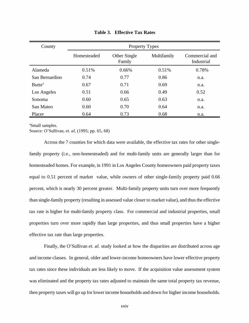
xxiv

Table 3. Effective Tax Rates

County Property Types

Homesteaded Other SingleFamily

Multifamily Commercial andIndustrial

Alameda 0.51% 0.66% 0.51% 0.78%

San Bernardino 0.74 0.77 0.86 n.a.

Buttea 0.67 0.71 0.69 n.a.

Los Angeles 0.51 0.66 0.49 0.52

Sonoma 0.60 0.65 0.63 n.a.

San Mateo 0.60 0.70 0.64 n.a.

Placer 0.64 0.73 0.68 n.a.

aSmall samples.Source: O’Sullivan, et. al, (1995; pp. 65, 68)

Across the 7 counties for which data were available, the effective tax rates for other single-

family property (i.e., non-homesteaded) and for multi-family units are generally larger than for

homesteaded homes. For example, in 1991 in Los Angeles County homeowners paid property taxes

equal to 0.51 percent of market value, while owners of other single-family property paid 0.66

percent, which is nearly 30 percent greater. Multi-family property units turn over more frequently

than single-family property (resulting in assessed value closer to market value), and thus the effective

tax rate is higher for multi-family property class. For commercial and industrial properties, small

properties turn over more rapidly than large properties, and thus small properties have a higher

effective tax rate than large properties.

Finally, the O’Sullivan et. al. study looked at how the disparities are distributed across age

and income classes. In general, older and lower-income homeowners have lower effective property

tax rates since these individuals are less likely to move. If the acquisition value assessment system

was eliminated and the property tax rates adjusted to maintain the same total property tax revenue,

then property taxes will go up for lower income households and down for higher income households.

xxv

For example, replacing the acquisition value with market value but maintaining the same property tax

revenue would increase property taxes for an average Los Angeles County homeowner in the $10,000

to $20,000 income bracket by $206, but decrease property taxes by $109 for a household in the

$80,000 to $90,000 income bracket (O’Sullivan et. al., 1995; p.74).

Older households also benefit from the acquisition value assessment system. Seniors in Los

Angeles County would pay an average of $503 more in property taxes while non-seniors would pay

$152 less if the acquisition value system was replaced with a market value assessment system.

These changes in property tax payments mask substantial variations within income classes and

within age groups. For example, within the $40,000 to $45,000 income range, the average tax

change in Los Angeles County from eliminating acquisition value assessments is close to zero, but

25 percent of the households within that income range would experience an average tax decrease of

$413 while 25 percent would experience a $417 tax increase (O’Sullivan, et. al., 1995; p. 75).

These results of O’Sullivan et. al. (1995) are consistent with earlier work focused on

Proposition 13. For example, Chernick and Reschovsky (1982) concluded that low-income

households and older households benefit from Proposition 13 and that substantial horizontal inequities

are created. Menchik et. al. (1982) also found that low-income homeowners benefit from acquisition

value assessment. Beaumont (1991) concludes that renters and younger people lose with the

adoption of acquisition value assessment.

C. Other Economics Effects of Acquisition Value Assessment

Acquisition value assessment creates or alters economic incentives. Such an assessment

system should reduce the likelihood that a home owner will move, i.e., it should discourage home

owners from selling their existing home and buying another one. The estimated effect on mobility,

however, is small. For households who are the least mobile, O’Sullivan et. al. (1994) estimate that

4Until recently, Georgia allowed amendments to the state constitution that apply to justspecific jurisdictions.

xxvi

the acquisition value assessment increases the time between move by 12 percent, or about a year on

average. For the most-mobile households, they find that the time between moves increases by only

1.2 percent.

V. Property Tax Assessment Limitation in Muscogee County

Beginning in 1983, as a result of a local constitutional amendment, the assessed values of

homesteaded property, i.e., property eligible for a homestead exemption, for local property tax

purposes were frozen in Muscogee County.4 The assessed value of such property can be increased

only if the property ownership changes (other than between spouses), there is an addition to or

renovation of the property, or to correct an error. Thus, for homesteaded property, Muscogee

County has a true acquisition value property tax system.

The limitation on assessment increases applies only to local property taxes. The state levies

a 0.25 mill property tax on 40 percent of the current fair market value, less any homestead

exemptions. Thus, the county must maintain two assessed values, the “frozen value” for local taxes

and the fair market value for state taxes, for each homesteaded property. By comparing these two

values, it is possible to determine how the freeze has effected property taxes in Muscogee County.

(We do not have to estimate market value as did O’Sullivan et. al.; we use the state assessed value.)

The analysis of this assessment freeze first considers the effect on the aggregate property tax

base, and then considers disparities across in assessments across individual parcels. The third part

of the analysis relates the assessed values within particular census tracts with the socio-economic

characteristics of the census tracts. Finally, we present estimates of the effect of the property tax

freeze on the probability of selling a home.

xxvii

A. The Effect on Aggregate Property Tax Digest

Tables 4 and 5 present annual data on the state and local property tax digest. The data for this

aggregate analysis were obtained from the Muscogee County Tax Commissioner. A few comments

about the data are in order. First, data prior to 1985 were not available. Second, the state

classification system for property changed in 1989. In particular, there were changes in the residential

category, and thus direct comparisons by category pre- and post-1989 are not feasible. Third, state

legislation passed in 1986 changed the way the state evaluates how well each county does in assessing

property, which resulted in counties changing how they conduct their assessments. As a result of the

legislation, nearly all counties had to conduct a mass re-assessment by 1989. Fourth, the local

(frozen) property tax base by property class was not available prior to 1989; in particular data for the

total local value of residential property are not available prior to 1989.

Table 4 shows the total gross digest and residential gross digest for state and for local

purposes by year. Consider first the total gross digest. For the years 1985 to 1988, the difference

between the state and local digest was small, $50 million or less. The freeze reduced gross assessed

value for local tax purposes by less than 3.5 percent in these years. During that period, property

assessments for state purposes did not change very much, so that the differences in state and local

digest remained small. The state digest changed dramatically in 1989, due in part to a mass

revaluation, while the local digest did not increase as much because of the freeze. For the post-1989

period, the assessment freeze resulted in differences between the state and local total gross digest in

the $165 to $200 million range, or by about 6 percent to about 10 percent. The dollar difference

between the state and gross local digest declined from 1989 to 1995, but has since increased by a

xxviii

Table 4

xxix

Table 5

xxx

modest amount. The percentage difference continuously declined between 1989 and 1997, falling

from 9.91 percent to 5.93 percent.

The reduction in the local gross property tax base due to the freeze is not very large; in recent

years the difference between that state and local gross digest equals about one year of growth in the

state (non-frozen) digest. For 1997, the ratio of assessed value for local purposes to assessed value

for state purposes is 0.94, which is much larger than the 1991 ratios reported in Table 2 for California

counties. The difference between Muscogee County and California is likely due to slower increases

in property values in Muscogee County and perhaps to more rapid turnover of homes.

For residential property, comparisons between state and local digest can be made only for the

post-1989 period. Nearly all property with a frozen value is classified as residential property; homes

that are part of a farm are included in the freeze but are not separated out from other agricultural

property. However, not all residential property is eligible for the freeze. Thus, about 95 percent of

the difference between the total gross state and local digest is accounted for by residential property.

Since the residential difference is approximately equal to the difference in the total gross digests, the

pattern for the differences between the state and local residential gross digests are similar to those for

total gross digests. This also suggests that for the pre-1990 period residential property followed the

pattern for the total gross digest. (The large change in the state residential gross digest between 1989

and 1990 is due in part to the change in how property is classified.) The difference in frozen and non-

frozen residential values is about 15 percent. Thus, on average the freeze has reduced residential

property taxes by 15 percent, assuming that the property tax rate was not increased to offset the

reduction in the tax base.

Table 5 presents information on the net digest, i.e., the gross digest less exemptions

(homestead and others). For Table 5, the state digest equals the gross state digest less the state-level

xxxi

exemptions, while the local digest equals the gross local digest less the local-level exemptions.

Muscogee County has much larger homestead exemptions than homestead allowed for the state

property taxes. For example, for 1997 the state allowed a regular homestead exemption of $2,000

for the state’s 0.25 mills property tax, while in Muscogee County the regular homestead exemption

for local property taxes was $13,500. Therefore, the difference between state and local total net

digest is much larger than for the total gross digest. In 1997, for example, the difference in the net

digests was $531 million, while the difference in gross digests was $178 million. Again, the patterns

for the differences for total net digest and for the residential proportion are very similar.

Relative to the reduction in local assessed value due to the exemptions, particularly the

homestead exemptions, the property tax freeze has had a relatively small effect on total taxable

property tax base in Muscogee County.

B. An Analysis of Assessment Disparities

In order to investigate disparities in assessment that result from the freeze, we obtained

individual parcels records for each year 1985 through 1997, with the exceptions of 1987, 1988, and

1991 for which the computer tapes could not be located. We focused the analysis on parcels that

were classified as residential; a few other parcels are eligible for the freeze but were not considered

in this analysis.

Table 6 presents a distribution of the ratio of local to state values in 1997 for all 33,265

parcels that are eligible for the freeze. This ratio is similar to the effective tax rate calculated for

California, except that in Georgia the property tax rate is not restricted to one percent, and thus is

not the effective property tax rate. But it is still the case that the smaller the ratio, the more that the

parcel benefits from the freeze. We separately consider properties that have a state assessed value

of more than $13,500 and less than or equal to $13,500 since $13,500 is the value of the homestead

xxxii

Table 6. Distribution of the Ratio of Local to State Value – 1997

Ratio of Localto State Value

Number of Parcelswith State Value

> $13,500

% of TotalParcels

Number of Parcelswith State Value

<= $13,500

% ofTotal

Parcels

Number ofParcels

% of TotalParcels

.90 to 1.0 12621 42.8% 1328 35.2% 13949 41.9%

.80 to .89 3248 11.0 324 8.6 3572 10.7

.70 to .79 2835 9.6 758 20.1 3593 10.8

.60 to .69 5743 19.5 815 21.6 6558 19.7

.50 to .59 4095 13.9 383 10.2 4478 13.5

.40 to .49 830 2.8 112 3.0 942 2.8

.30 to .39 105 0.4 36 1.0 141 0.4

.20 to .29 11 0.0 13 0.3 24 0.1

.10 to .19 6 0.0 2 0.1 8 0.0

0 to .09 0 0.0 0 0.0 0 0.0

exemption. Thus, property with a state assessed value of $13,500 or less would not be affected by

the freeze.

As can be seen in Table 6, there are substantial disparities in assessment due to the freeze.

While 42.8 percent of parcels with assessed values over $13,500 have ratios of local to state values

between 0.9 and 1.0, the remaining approximately 60 percent of parcels have local to state value

ratios that range from 0.10 to 0.89, with the bulk lying between 0.50 and 0.89.

Table 7 shows how the effect of the freeze varies with the year that the property last became

eligible for the freeze. Table 7 starts with parcels that in 1997 were eligible for the freeze, i.e., were

homesteaded. We then determined the year in which each parcel took on its 1997 local value, i.e.,

we identified the year in which the parcel’s assessed value was last frozen. The number of parcels

frozen in each year is shown in column one. Of the parcels that have frozen values in 1997, 28.7

percent were first frozen in 1985 or earlier (data was not available for 1984.) In Los Angeles

xxxiii

Table 7. State and Local Values

Year Parcels by Year property took1997 local value

Median 1997 Value Disparity Ratio

Number Percent State Local

1997 1652 4.97 $30,164 $25,647 1.18

1996 1571 4.72 $29,366 $24,839 1.18

1995 1723 5.18 $27,234 $23,452 1.16

1994 1762 5.30 $27,774 $24,699 1.12

1993 1770 5.32 $26,478 $24,601 1.07

1992 3088 9.28 $24,413 $22,114 1.10

1991

1990 2113 6.35 $25,326 $23,103 1.10

1989 8155 24.52 $25,763 $21,630 1.19

1988

1987

1986 1868 5.62 $25,845 $21,840 1.18

1985 9557 28.74 $20,753 $12,440 1.67

County, 33.2 percent of the parcels took their current (1996) value in 1975. Given that the time

period for Los Angeles County is longer than for Muscogee County, the 28.7 percent is low. This

suggests that there is more turnover of housing in Muscogee County than in Los Angeles County.

Columns 3 and 4 give the 1997 median state and local value for parcels who assessments were

first frozen in that year. The state value of the parcels increased over time. The last column contains

the disparity ratio and shows how differences between the state and local value increase the longer

the parcels’ local assessed value has been frozen. These ratios are similar to the ratios for California

as shown in Table 1.

For parcels that were first frozen in 1985 or 1984, the disparity ratio is 1.67. The 1991

disparity ratios for 1975 for California counties, as reported in Table 2, are much higher than that.

This is partly due to the shorter duration of the Muscogee County freeze and the smaller increases

xxxiv

in property values in Muscogee County. For Los Angeles County, property that has been frozen

since 1982, i.e., the same elapse time as the Muscogee freeze has been in effect, has a disparity ratio

for 1996 of 1.27. This is lower than for Muscogee County, reflecting the decline in property values

in California during the 1990s. The disparity ratio for Muscogee County decreases the shorter the

time the parcel has been frozen, but the change since 1989 is very small.

Table 8 shows the difference for 1997 between the state (non-frozen) assessed value and the

local (frozen) assessed value by assessed value categories. The first column shows the total number

of residential parcels, while column two shows the average assessed value for state tax purposes for

all residential parcels. Residential parcels include rental homes and complexes of four units or less.

Thus, not all property classified as residential are homestead property, i.e., eligible for the freeze.

Column 3 shows the number of parcels with frozen values, and the next two columns present

the average assessed value for state purposes (i.e., the non-frozen value) and the average assessed

value for local purposes (i.e., the frozen value).

Columns 6 and 7 show the mean total and percentage differences between the state and local

values. (Note these values are the difference between the average assessed values, not the mean of

the differences.) The average reduction in assessed value due to the freeze is much larger for the

higher valued properties than for lower valued properties. For example, for parcels whose state

assessed value is between $200,000 and $300,000 the reduction is 11.2 times the reduction for

properties with a state assessed value of less than $25,000. However, expressed as a percentage

reduction in assessed value, the relatively larger reductions occur for the low and high valued

residential units. The parcels in the two highest valued classes, for which state and local values are

the same, are homes that have recently been built or sold.

xxxv

Table 8

xxxvi

The last two columns of Table 8 presents the maximum differences (in dollars and

percentages) for a single parcel within in each assessed value class. The pattern for the maximum

dollar difference is very similar to that for the differences in mean values, although the dollar

differences for higher valued homes relative to that for lower valued homes is not as great as for the

mean difference. For lower valued homes there are parcels whose local assessment is 80 to 85

percent lower than their state assessment.

C. An Analysis by Socio-Economic Characteristic

No information concerning the characteristics of homeowners is available in the property tax

files. In order to relate the freeze to socio-economic characteristics we relied on census tract data

from the 1990 Census of Population. We first identified the census tract for each of the residential

parcels. We then regressed the mean value of the difference between fair market value and the frozen

value (both dollars and percentage) against each socio-economic characteristics of the census tracts.

Table 9 contains the results of the six regressions. The average dollar reduction within a

census tract in assessed value due to the freeze increases with income, age, and percent white. Thus,

the elimination of the freeze would increase assessed values more for higher income homeowners,

for the elderly, and for whites. Recall that O’Sullivan et. al. (1995) found that lower income and

elderly homeowners would be worse off if the assessment limitation was removed in California.

In terms of the percentage reduction the results are just the opposite for income, i.e., higher

income homeowners have a smaller percentage reduction in assessed value due to the freeze. Median

age and percent white are not statistically significant in the regressions with percentage reduction in

assessed value.

xxxvii

Table 9. Regressions with Socio-Economic Characteristics

Dependent Variable: Difference Between State and Local Assessed Value

Independent Variables

Dollar Difference Percentage Difference

MedianIncome

Mean Age PercentWhite

MedianIncome

Mean Age PercentWhite

Intercept 14674.4 27.04 36.173 47,456.5 28.79 81.92

Coefficient 2.00 .001 0.005 -113,447 25.12 -109.01

t-statistic 2.69 4.59 2.95 3.13 1.33 1.22

R2 0.128 0.300 0.151 0.167 0.035 0.029

Sample size = 51

D. Mobility

We explored the effect of the freeze on the probability that a homeowner would move by

estimating a probit regression for moves in 1997. We expect that the probability of moving should

be negatively related to the absolute difference between the state and local assessed value, denoted

DIFF. In other words, we expect that the benefit of the freeze would lock-in homeowners, thereby

reducing the probability of moving. For control variables we included a set of dummies to measure

the number of years that the homeowner has occupied the house. We include these variables to

capture the effect that duration might have on the probability of moving. Since occupancy duration

is truncated at 1986 and since we have no expectation that the effect of duration will be linear, we

used a set of dummy variables, denoted D1996 through D1985, to measure duration. The value of

D1996 equals one if the owner moved into the house in 1996, etc. The excluded dummy is D1985,

which equals one if the owner moved into the home in 1985 or earlier. To control for socio-

economic characteristics we included a set of variables measured at the census tract level. These

variables and the expected signs are:

xxxviii

• Population (POP) is included to control for the size of the census tract; we have no apriori expectation regarding the sign of the coefficient.

• Median age (AGE) is included since we expect that older individuals are less likely tomove, implying a negative sign.

• Percent white (%WH) is included since we expect whites to move more frequently thannonwhites because of less restrictions on housing choices due to discrimination, and thuswe expect a positive sign.

• Households with higher median income (INC) are expected to move more frequently, andthus we expect a positive sign.

• The percent who lived in the census tract in 1985 (SAME) is included to control forneighborhood stability; it should be negatively related to the probability that someone inthe census tract will move and thus we expect a negative sign.

• Percent owner occupied housing (%OWN) is included as another measure of the stabilityof the neighborhood; we expect the sign to be negative.

• We expect that homes in census tracts with higher median house value (VALUE) to be

more likely to move, so we expect a positive sign.

Table 10 contains the regression results.

The results in Table 10 suggest that the probability of moving is unrelated to the value of the

freeze. We had expected that the coefficient on DIFF would be negative, but it is positive but is not

statistically significant. The coefficients on the duration variables are all negative and generally

significant. The negative coefficients on the duration dummies imply that the probability of moving

is less if one moved into the home after 1985. However, the coefficients on the duration dummies

do not follow any particular pattern.

The control variables are all significant, with the exception of %OWN. The signs of the

coefficients are generally what one might expect, except for %WH and VALUE.

xxxix

Table 10. Probit Equations for Moving

Variable Coefficient Standard Error

Intercept 1.710 0.111*

DIFF 0.018 0.040

D1996 -0.179 0.042*

D1995 -0.094 0.044**

D1994 -0.095 0.047**

D1993 -0.075 0.050

D1992 -0.151 0.043*

D1990 -0.026 0.057

D1989 -0.064 0.036***

D1986 -0.247 0.063*

POP (in 1000s) 0.024 .007*

AGE -0.024 0.005*

%WH -0.001 0.0006**

INC (in 1000s) 0.013 0.004*

SAME 0.011 0.003*

%OWN -0.002 0.002

VALUE (in 1000s) -0.002 0.001**

Log Likelihood = -7872.42

* significant at the 1 percent level** significant a the 5 percent level*** significant at the 10 percent level

xl

We estimated similar equations for each year. We also estimated the equation using the

percentage differences in state and local assessed values, and with different combinations of the

control variables. In none of the regressions was the benefit of the freeze statistically significant.

VI. Conclusions

No one looks forward to tax increases, especially increases in taxes that result from an

increase in unrealized property value. While a household’s wealth increased as property value

increases, there has not necessarily been an increase in the household’s cash flow to pay the taxes.

Thus, pressure is exerted to impose controls on the increase in property taxes. But limitations on

increases in property tax assessments results in large disparities in property taxes. Furthermore,

assessments limitations do little to increase the stability of communities since the effect on mobility

is small.

xli

References

Advisory Commission on Intergovernmental Relations, Tax and Expenditure Limits on LocalGovernment. Washington, D.C.: U.S. Advisory Commission on Intergovernmental Relations,1995.

Beaumont, Marion S., “Proposition 13 Winners and Losers: Where First-Time Buyers AffectedAdversely?” in Frederick D. Stocker (ed), Proposition 13: A Ten-Year RetrospectiveCambridge, MA: The Lincoln Institute of Land Policy, 1991.

Chernick, Howard, and Andrew Reschovsky, “The Distributional Impact of Proposition 13: AMicrosimulation Approach.” National Tax Journal, 2, June 1982: pp. 149-170.

Downes, Thomas A., and David N. Figlio, 1999, “Do Tax and Expenditure Limits Provide a FreeLunch? Evidence on the Link Between Limits and Public Sector Service Quality.” NationalTax Journal, 52(1): 113-128.

McGuire, Therese J., 1999, “Proposition 13 and Its Offspring: For Good or for Evil?” National TaxJournal, 52(1): 129-138.

Menchik, Mark David, Anthony Pascal, Dennis De Tray, Judith Fernandez, and Michael Caggiano,“Fiscal Restraint in Local Government: A Summary of Research Findings.” (Santa Monica:)The Rand Corporation; April 1995.

Mullins, Daniel, and Philip G.Joyce, “Tax and Expenditure Limitations and State and Local FiscalStructure: An Empirical Assessment.” Public Budgeting and Finance, 15, Spring 1996: pp.75-101.

O’Sullivan, Arthur, Terri A. Sexton, and Steven M. Sheffrin, Property Taxes & Tax Revolts: TheLegacy of Proposition 13. New York: Cambridge University Press, 1995.

Preston, Anne E., and Casey Ichniowski. 1991. “A National Perspective on the Nature and Effectsof the Local Property Tax Revolt, 1976-1986,” National Tax Journal 44(2): 123-45.

Shadbegian, Ronald J., 1998, “Do Tax and Expenditures Limitations Affect Local GovernmentBudgets? Evidence from Panel Data.” Public Finance Review 26 (2): 218-36.

Shadbegian, Ronald J., 1999, “The Effect of Tax and Expenditures Limitations on the RevenueStructure of Local Government, 1962-87.” National Tax Journal 52 (2): 221-37.

Sheffrin, Steven M., and Terri Sexton, 1998, Proposition 13 in Recession and Recovery. SanFrancisco: Public Policy Institute of California.

xlii

ABOUT THE AUTHORS

David L. Sjoquist is Professor of Economics and Director in the Fiscal Research Program of

the Andrew Young School of Policy Studies at Georgia State University. He has published widely

on topics related to state and local public finance and urban economics. He holds a Ph.D. from the

University of Minnesota.

Lakshmi Pandey is Administrative Manager and Data Manager in the Fiscal Research

Program of the Andrew Young School of Policy Studies at Georgia State University. He holds B.S.,

M.S. and Ph.D. in Physics from Banaras Hindu University, India. Dr. Pandey has published over 80

papers in the field of physics.

ABOUT THE FISCAL RESEARCH PROGRAM

The Fiscal Research Program provides nonpartisan research, technical assistance, and

education in the evaluation and design of state and local fiscal and economic policy, including both

tax and expenditure issues. The Program’s mission is to promote development of sound public policy

and public understanding of issues of concern to state and local governments.

The Fiscal Research Program (FRP) was established in 1995 in order to provide a stronger

research foundation for setting fiscal policy for state and local governments and for better informed

decision making. The FRP, one of several prominent policy research centers and academic

departments housed in the School of Policy Studies, has a full-time staff and affiliated faculty from

throughout Georgia State University and elsewhere who lead the research efforts in many organized

projects.

The FRP maintains a position of neutrality on public policy issues in order to safeguard the

academic freedom of authors. Thus, interpretations or conclusions in FRP publications should be

understood to be solely those of the author.

xliii

FISCAL RESEARCH PROGRAM

David L. Sjoquist, Director and Professor of EconomicsRoy W. Bahl, Dean and Professor of Economics

Mary K. Bumgarner, Principal AssociateRichard W. Campbell, Principal Associate

Gary Cornia, Principal AssociateRonald G. Cummings, Professor of Economics

Dwight R. Doering, Research AssociateKelly D. Edmiston, Assistant Professor of Economics

Dagney G. Faulk, Research AssociateMichael E. Foster, Associate Professor of Public Administration and Nursing

Martin F. Grace, Associate Professor of Risk Management and Insurance Richard R. Hawkins, Principal Associate

Julie Hotchkiss, Associate Professor of EconomicsL. Kenneth Hubbell, Principal Associate

Keith R. Ihlanfeldt, Professor of EconomicsErnest R. Larkin, Professor of Accountancy

Gregory B. Lewis, Professor of Public Administration and Urban StudiesJorge L. Martinez-Vazquez, Professor of Economics

Julia E. Melkers, Assistant Professor of Public AdministrationJack Morton, Principal Associate

Lakshmi N. Pandey, Research AssociateTheodore H. Poister, Professor of Public Administration

Donald Ratajczak, Regents’ Professor of EconomicsRoss H. Rubenstein, Assistant Professor of Public Admin. and Educational Policy Studies

Francis W. Rushing, Professor of EconomicsBenjamin P. Scafidi, Assistant Professor of EconomicsBruce A. Seaman, Associate Professor of Economics

Saloua Sehili, Principal AssociateSamuel L. Skogstad, Chair and Professor of Economics

William J. Smith, Research AssociateStanley J. Smits, Principal AssociateJeanie J. Thomas, Research Associate

Sally Wallace, Assistant Professor of EconomicsMary Beth Walker, Associate Professor of Economics

Thomas L. Weyandt, Senior Associate and Executive Director Research Atlanta Inc.Laura Wheeler, Principal Associate

Katherine G. Willoughby, Associate Professor of Economics

StaffDorie Taylor, Associate to the DirectorMargo Doers, Administrative Support

Graduate Research AssistantsHsin-hui ChuiRobbie Collins

Natalia DyominaKiran Hebbar

John MatthewsMary Kathleen Thomas

H. Christina Yang

xliv

RECENT PUBLICATIONS OF THE FISCAL RESEARCH PROGRAM(All publications listed are available through the FRP)

Limitations on Increases in Property Tax Assessed Value.(David L. Sjoquist and Lakshmi Pandey)

This report describes how various states limit the growth in property tax assessment and explores theimplications of such limitations. FRP Report/Brief 37 (November 1999).

Corporate Tax Credits Considered for Social Policy.(DagneyFaulk)

An update on budget and policy issues affecting Georgia’s children and families. Prepared for “FiscalFact” a publication of Georgians for Children. FRP Report 36 (September 1999).

Manufactured Housing in Georgia: Trends and Fiscal Implications. (L. Kenneth Hubbell and David L. Sjoquist)

This report discusses the growth of manufactured housing and explores the implications for theproperty tax base. FRP Report/Brief 35 (September 1999).

An Analysis of Franchise Fees in Georgia. (Bruce Seaman)This report examines the current structure of franchise fees, identifies the associated problems, and

describes options for addressing the problems. FRP Report 34 (August 1999).

Road Construction and Regional Development. (Felix Rioja)This report investigates the effect of roads on economic development. FRP Report/Brief 33 (July1999).

Distribution of Public Education Funding in Georgia, 1992: Equity From a National Perspective. (Ross H. Rubenstein, Dwight R. Doering and Michelle Moser)

This report compares the inter-district equity of school revenue in Georgia with that of all other states.FRP Report/Brief 32 (April 1999).

The New Local Revenue Roller Coaster: Growth and Stability Implications for Increasing Local Sales TaxReliance in Georgia. (Richard Hawkins)

This report examines the relative growth and stability of the property tax and local sales tax basesacross counties in Georgia. FRP Report/Brief 31 (March 1999).

Results of Georgia Statewide Poll – Economic Development. (Applied Research Center/Fiscal ResearchProgram)

This report prepared for the Georgia Economic Developers Association presents results of a surveyon economic development activities in the state. FRP Report 30 (March 1999).

State and Local Government Taxation of Manufactured Housing (L. Kenneth Hubbell)This report is a 50 state comparison of property and sales tax treatment of manufactured housing.FRP Report 29 (February 1999)

Handbook on Taxation, 5th Edition (Jack Morton and Richard Hawkins)A quick overview of all state and local taxes in Georgia. FRP Annual Publication A(5)(January 1999)

xlv

RECENT FRP PUBLICATIONS (Continued)

Exemptions From Sales and Use Tax: Solid Fuels Used by Manufacturing Firms (William J. Smith)This brief discusses the issues and revenue loss associated with exemptions in solid fuel from salestaxation. FRP Brief 28 (January 1999)

Economic Development Policy (Keith Ihlanfeldt)This report addresses five weaknesses in Georgia’s economic development program and recommendspolicies to overcome these weaknesses. FRP Report/Brief 27 (January 1999)

The Manipulation of State Corporate Income Tax Apportionment Formulas As An Economic DevelopmentTool (Kelly Edmiston)

This paper uses a simulation model to examine the effects of disproportionate sales factor weightingin state corporate income tax apportionment formulas on economic development, tax collections, andregional welfare. FRP Brief 26 (November 1998)

The Impact of House Bill No. 129 on Funding for Central Administration in the School Districts of Georgia(Dwight R. Doering)

This report presents an analysis of the impact of HB 129 on the funding of the central administrationfunction in Georgia’s school districts. FRP Brief 25 (November 1998)

Revenue Losses from Exemptions of Goods from the Georgia Sales Tax (Mary Beth Walker)This report presents estimates of the loss of revenue from exemptions of specific goods or classes ofgoods from the sales tax base. FRP Brief 24 (November 1998)

The Equity of Public Education Funding in Georgia, 1988-1996 (Ross H. Rubenstein, Dwight R. Doeringand Larry R. Gess)

A study of the effect of Quality Basic Education on the level of equity of public education funding inGeorgia. FRP Report/Brief 23 (October 1998)

An Analysis of the Barnes and Millner Property Tax Relief Proposals (David L. Sjoquist)An analysis prepared for the Georgia Public Policy Foundation, FRP Report 22 (October 1998) alsoavailable from the Georgia Public Policy Foundation, Kelly McCutchen, 770/455-7600.

A Review of Georgia’s Quality Basic Education Formula Fiscal Year 1987 Through 1998 (Dwight R. Doering and Larry R. Gess)

A review of how funding per student for each formula component of Quality Basic Education (QBE)changed between 1987 and 1998. FRP Brief 21 (September 1998)

Net Fiscal Incidence at the Regional Level: A Computable General Equilibrium Model with Voting(Saloua Sehili)

An analysis of the net incidence of expenditures and taxes in Georgia using a computable generalequilibrium model. FRP Report 20 (September 1998)

An Analysis of the Economic Consequences of Modifying the Property Tax on Motor Vehicles in Georgia:Alternative Proposals and Revenue Effects (Laura A. Wheeler)

An analysis of revenue effects and distribution consequences on eliminating tax on motor vehicles.FRP Report/Brief 19 (September 1998)

xlvi

RECENT FRP PUBLICATIONS (Continued)

The Taxation of Personal Property in Georgia (Dagney Faulk)A policy option for changing how Georgia taxes personal property. FRP Report/Brief 18 (August1998)

Insurance Taxation in Georgia: Analysis and Options (Martin F. Grace)An overview of issues associated with the taxation of the insurance industry in Georgia.FRP Report/Brief 17 (August 1998).

The Structure of School Districts in Georgia: Economies of Scale and Determinants of Consolidation(L.F. Jameson Boex and Jorge Martinez-Vasquez)

An analysis of economies of scale in primary and secondary education in Georgia and its relation toschool district consolidation. FRP Report/Brief 16 (July 1998).

Georgia’s Job Tax Credit: An Analysis of the Characteristics of Eligible Firms (Dagney Faulk)This report provides a review of Georgia’s Job Tax Credit and makes recommendations for improvingthe JTC program. FRP Report/Brief 8 (June 1998).

Performance Based Budgeting Requirements in State Governments (Julia Melkers and Katherine G. Willoughby)

This policy brief addresses the trend toward improving performance in state government through theuse of performance-based budgeting. FRP Brief 7 (June 1998).

Interdistrict School Choice in Georgia: Issues of Equity (Dwight Robert Doering)A description of the interdistrict school choice programs in Georgia with a focus on equity issues.FRP Report/Brief 6 (May 1998).

A Comparative Analysis of Southeastern States Income Tax Treatment of Exporters (Ernest R. Larkins,Jorge Martinez-Vasquez, and John J. Masselli)

This study analyzes the export-related provisions of tax laws and proposes policy changes. FRPReport 15 (May 1998).

Reducing the Property Tax on Motor Vehicles in Georgia (Laura Wheeler)An analysis prepared for the Georgia Public Policy Foundation, FRP Report 14 (June 1998) alsoavailable from the Georgia Public Policy Foundation, Kelly McCutchen, 770/455-7600.

Georgia’s Corporate Taxes: Should the Corporate Income Tax be Repealed? (Martin F. Grace)An analysis prepared for the Georgia Public Policy Foundation, FRP Report 13 (April 1998) alsoavailable from the Georgia Public Policy Foundation, Kelly McCutchen, 770/455-7600.

The Georgia Individual Tax: Current Structure and Impact of Proposed Changes (Barbara M. Edwards)An analysis prepared for the Georgia Public Policy Foundation, FRP Report 12 (April 1998) alsoavailable from the Georgia Public Policy Foundation, Kelly McCutchen, 770/455-7600.

A Georgia Sales Tax for the 21st Century (Roy Bahl and Richard Hawkins)An analysis prepared for the Georgia Public Policy Foundation FRP Report 11 (April 1998) alsoavailable from the Georgia Public Policy Foundation, Kelly McCutchen, 770/455-7600.

xlvii

RECENT FRP PUBLICATIONS (Continued)

Results of Georgia Statewide Poll -- Economic Development (Applied Research Center/Fiscal ResearchProgram)

This report prepared for the Georgia Economic Developers Association presents results of a surveyon economic development activities in the state. FRP Report 10 (April 1998).

Georgia’s Revenue Shortfall Reserve: An Analysis of its Role, Size and Structure (David L. Sjoquist)This report explores Georgia’s “rainy day” fund. FRP Report/Brief 5 (March 1998).

Natural Gas Deregulation and State Sales Tax Collections in Georgia (Richard R. Hawkins)This policy brief discusses the issues that will ultimately determine the impact on sales tax revenue inGeorgia resulting from deregulation of the natural gas industry. FRP Brief 4 (February 1998).

Creating the Workforce of the Future: A Requirements Analysis (Francis W. Rushing and Stanley J. Smits)This paper focuses on the theme of workforce preparation. FRP Report/Brief 3 (February 1998).

Economic and Community Development Research in Georgia Colleges and Universities, An AnnotatedBibliography (Fiscal Research Program)

An annotation of work authored within the last ten years. FRP Report 9 (January 1998).

The Georgia Income Tax: Suggestions and Analysis for Reform (Sally Wallace and Barbara M. Edwards)An examination of the state income tax and suggestions for reform. FRP Report/Brief 2 (November1997).

The Sales Tax in Georgia: Issues and Options (Roy Bahl and Richard Hawkins)An overview of the sales tax and policy options. FRP Report/Brief 1 (October 1997).

Economies of Scale in Property Tax Assessment (David L. Sjoquist and Mary Beth Walker)An analysis of the relationship in Georgia between the cost of property tax assessment and county size.FRP Report 97.2 (September 1997).

Sales Taxation of Telecommunications Services in the State of Utah (Richard McHugh)An analysis of the sales and use taxation of telecommunications services with specific reference toUtah. FRP Report 97.1 (February 1997).

Local Government Fiscal Effort (David L. Sjoquist)An analysis prepared for the Georgia Future Communities Commission comparing the fiscal capabilityand actual revenues for Georgia counties and municipalities. FRP Report 96.5 (December 1996).

Georgia Banking: An Overview (Samuel Skogstad)A description of the current Georgia regulatory environment for the banking industry. FRP Report96.4 (May 1996).

xlviii

RECENT FRP PUBLICATIONS (Continued)

Telecommunication Taxation: The Georgia Case (Richard McHugh)An examination and assessment of the current structure of telecommunications taxation in Georgia. FRP Report 96.3 (May 1996).

Local Government Fiscal Viability (David L. Sjoquist)An analysis prepared for the Georgia Future Communities Commission of the fiscal capacity,expenditure needs and fiscal viability of counties across Georgia. FRP Report 96.2 (March 1996).

Taxation and Economic Development: A Blueprint for Tax Reform in Ohio (Roy Bahl, ed.)A collection of reports prepared for the Ohio Blue Ribbon Commission on Taxation and EconomicDevelopment. FRP Report 96.6 (1996) available only from Battelle Press, $44.95, 800/451-3543.

Reflections on Privatization (Steve Hanke)An overview of the economic and policy fundamentals of privatization. FRP Report 95.2 (March1996).

Reforming the Georgia Tax Structure (Roy Bahl)The final report of the Joint Study Commission on Revenue Structure. FRP Report 95.1 (January1995).

For a free copy of any of the publications listed, call the FRP at 404/651-4342, or fax us at 404/651-2737.

xlix

FORTHCOMING AND IN-PROCESS REPORTS

Changes in the Geographic Distribution of Income in Georgia (Robbie Collins)

The Changing Geographic Pattern of Retail Sales in Georgia (Joey Smith)

The Effect of Structural Changes in the Banking Industry on the Availability of Financing (Dileep Mehta)

The Link Between the State Budget and State Policy (William Thomas)

Property Tax Credits (David Sjoquist and Joey Smith)

Welfare-to-Work: Tracking the Budget Savings (James Wolk)