Limitations and Constraints of Eddy-Current Loss Models for IPM Motors with Fractional ... ·...
20
Article Limitations and Constraints of Eddy-Current Loss Models for IPM Motors with Fractional-Slot Concentrated Windings Hui Zhang and Oskar Wallmark * Department of Electric Power and Energy Systems, KTH Royal Institute of Technology, SE-100 44 Stockholm, Sweden; [email protected] * Correspondence: [email protected]; Tel.: +46-8-790-78-31 Abstract: This paper analyzes and compares models for predicting average magnet losses in interior permanent-magnet motors with fractional-slot concentrated windings due to harmonics in the armature reaction (assuming sinusoidal phase currents). Particularly, loss models adopting different formulations and solutions to the Helmholtz equation to solve for the eddy currents are compared to a simpler model relying on an assumed eddy-current distribution. Boundaries in terms of magnet dimensions and angular frequency are identified (numerically and using an identified approximate analytical expression) to aid the machine designer whether the more simple loss model is applicable or not. The assumption of a uniform flux-density variation (used in the loss models) is also investigated for the case of V-shaped and straight interior permanent magnets. Finally, predicted volumetric loss densities are exemplified for combinations of slot and pole numbers common in automotive applications. Keywords: automotive applications; concentrated windings; eddy current losses; fractional-slot windings; interior permanent-magnet motors 1. Introduction In interior permanent-magnet motors (IPMs), the permanent magnets (PMs) are embedded into the rotor. Compared to rotors with surface-mounted PMs, the resulting flux concentration effect in IPMs significantly reduces the induced PM eddy-current losses caused by the changing air-gap permeance due to the slot openings. Further, a not insignificant magnetic saliency can be realized, which contributes with a reluctance torque component and thereby increases the torque density. These are two main reasons why the IPM is a common machine topology when targeting automotive applications, with recent examples including [1–7]. A fractional-slot concentrated winding (FSCW) enables very short end-winding lengths and, thereby, potential improvements in terms of torque density. However, depending on the combination of the number of stator slots Q s and poles p, the resulting harmonic content in the air-gap magnetomotive force (MMF) caused by the stator currents can be substantial. During the last decade, efforts were put into identifying suitable combinations of Q s and p where the impact of the stator MMF harmonics is as small as possible [8–10]. Particularly, for rotors with surface-mounted PMs, a number of models to quantify the induced eddy-current losses in the PMs based on the harmonic content in the stator MMF were developed [11–14]. Today, the combinations of Q s and p with the lowest harmonic content have been identified, and FSCWs are adopted in automotive applications (see, e.g., [15] and the references in [16]). However, while the above loss models indeed are useful, they are most suitable for comparing the relative change in eddy-current losses for different combinations of Q s and p rather than accurately predicting the losses for given PM dimensions. Particularly, the effect of segmentation of the magnets and the impact of the skin effect is challenging. Additionally, these models target surface-mounted PMs rather than IPMs. Having a good approximation of the resulting PM losses is important for the Preprints (www.preprints.org) | NOT PEER-REVIEWED | Posted: 16 March 2017 doi:10.20944/preprints201703.0113.v1 Peer-reviewed version available at Energies 2017, 10, 379; doi:10.3390/en10030379
Transcript of Limitations and Constraints of Eddy-Current Loss Models for IPM Motors with Fractional ... ·...
Article
Limitations and Constraints of Eddy-Current LossModels for IPM Motors with Fractional-SlotConcentrated Windings
Hui Zhang and Oskar Wallmark *
Department of Electric Power and Energy Systems, KTH Royal Institute of Technology,SE-100 44 Stockholm, Sweden; [email protected]* Correspondence: [email protected]; Tel.: +46-8-790-78-31
Abstract: This paper analyzes and compares models for predicting average magnet losses in interiorpermanent-magnet motors with fractional-slot concentrated windings due to harmonics in thearmature reaction (assuming sinusoidal phase currents). Particularly, loss models adopting differentformulations and solutions to the Helmholtz equation to solve for the eddy currents are comparedto a simpler model relying on an assumed eddy-current distribution. Boundaries in terms ofmagnet dimensions and angular frequency are identified (numerically and using an identifiedapproximate analytical expression) to aid the machine designer whether the more simple loss modelis applicable or not. The assumption of a uniform flux-density variation (used in the loss models) isalso investigated for the case of V-shaped and straight interior permanent magnets. Finally, predictedvolumetric loss densities are exemplified for combinations of slot and pole numbers common inautomotive applications.
Keywords: automotive applications; concentrated windings; eddy current losses; fractional-slotwindings; interior permanent-magnet motors
1. Introduction
In interior permanent-magnet motors (IPMs), the permanent magnets (PMs) are embedded intothe rotor. Compared to rotors with surface-mounted PMs, the resulting flux concentration effectin IPMs significantly reduces the induced PM eddy-current losses caused by the changing air-gappermeance due to the slot openings. Further, a not insignificant magnetic saliency can be realized,which contributes with a reluctance torque component and thereby increases the torque density.These are two main reasons why the IPM is a common machine topology when targeting automotiveapplications, with recent examples including [1–7].
A fractional-slot concentrated winding (FSCW) enables very short end-winding lengths and,thereby, potential improvements in terms of torque density. However, depending on the combination ofthe number of stator slots Qs and poles p, the resulting harmonic content in the air-gap magnetomotiveforce (MMF) caused by the stator currents can be substantial. During the last decade, efforts were putinto identifying suitable combinations of Qs and p where the impact of the stator MMF harmonics isas small as possible [8–10]. Particularly, for rotors with surface-mounted PMs, a number of models toquantify the induced eddy-current losses in the PMs based on the harmonic content in the stator MMFwere developed [11–14]. Today, the combinations of Qs and p with the lowest harmonic content havebeen identified, and FSCWs are adopted in automotive applications (see, e.g., [15] and the referencesin [16]).
However, while the above loss models indeed are useful, they are most suitable for comparingthe relative change in eddy-current losses for different combinations of Qs and p rather than accuratelypredicting the losses for given PM dimensions. Particularly, the effect of segmentation of the magnetsand the impact of the skin effect is challenging. Additionally, these models target surface-mountedPMs rather than IPMs. Having a good approximation of the resulting PM losses is important for the
Preprints (www.preprints.org) | NOT PEER-REVIEWED | Posted: 16 March 2017 doi:10.20944/preprints201703.0113.v1
Peer-reviewed version available at Energies 2017, 10, 379; doi:10.3390/en10030379
2 of 20
machine designer since relatively small losses in the PMs can result in excessive temperatures due tothe difficulty of transferring the resulting heat across the air gap.
Version February 26, 2017 submitted to Energies 2 of 20
However, while the above loss models indeed are useful, they are most suitable for comparing32
the relative change in eddy-current losses for different combinations of Qs and p rather than33
accurately predicting the losses for given PM dimensions. Particularly, the effect of segmentation34
of the magnets and the impact of the skin effect is challenging. Additionally, these models target35
surface-mounted PMs rather than IPMs. Having a good approximation of the resulting PM losses36
is important for the machine designer since relatively small losses in the PMs can result in excessive37
temperatures due to the difficulty of transferring the resulting heat across the air gap.
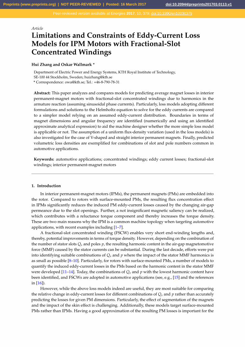
Figure 1. Sample FSCW-IPM with Qs =12 slots and p=8 poles.
38
Essentially, predicting the losses in the PMs can be done accurately using three-dimensional (3D)39
finite-element (FEM) based simulations (as demonstrated in [17]). However, the approach must still40
be considered relatively time consuming although efforts have been made to reduce the computation41
times [18]. Recently, the relatively simple analytical loss model in [19] was proposed considering42
FSCWs with surface-mounted PMs and including the effect of both axial and tangential segmentation43
of the PMs. This model uses the stator MMF harmonic content as input but neglects the impact of the44
skin effect. A more advanced model, incorporating the effect of axial and tangential segmentation as45
well as the skin effect, is adopted in [20] where analytical solutions of Helmholtz equation with an46
imposed source term are adopted. A different model (also accounting for segmentation and the skin47
effect) is adopted in [21] where solutions to Helmholtz equation with a prescribed boundary surface48
current are used.49
1.1. Contributions and Outline of Paper50
An overall aim of this work is to provide a link between models describing the harmonic content51
in FSCWs due to the stator MMF with corresponding, sufficiently accurate PM eddy-current loss52
models for IPMs. Particularly, the loss models in [20] (here designated Model B) and [21] (here53
designated Model C), adopting solutions to different formulations of Helmholtz equation to solve54
for the eddy currents, are compared to the considerably less complex loss model in [19] (here adapted55
to IPMs and designated Model A). It is demonstrated that Model B and Model C, though considerably56
different in terms of implementation complexity, predict very similar results (in good agreement57
with corresponding 3D-FEM simulations) for PM dimension and rotor speed intervals typically58
found in automotive applications. Further, limits (in terms of frequency and PM dimensions)59
where Model A (the least complex loss model) is applicable are identified numerically and using60
an approximate analytical expression. This limit is not straight forward since the rectangular shape61
of the PM segments results in complex eddy-current reaction fields. Key concepts regarding FSCWs62
are included as an appendix representing a complete description on how the uniform variation of63
the flux density in the PMs can be analytically predicted. The assumption of a uniform flux-density64
variation (used in the loss models) is also investigated for the case of V-shaped and straight interior65
permanent magnets. An extensive numerical evaluation using 3D-FEM based simulations is carried66
Figure 1. Sample fractional-slot concentrated winding (FSCW)-interior permanent-magnet motor (IPM)with Qs =12 slots and p=8 poles.
Essentially, predicting the losses in the PMs can be done accurately using three-dimensional (3D)finite-element (FEM)-based simulations (as demonstrated in [17]). However, the approach must still beconsidered relatively time consuming, although efforts have been made to reduce the computationtimes [18]. Recently, the relatively simple analytical loss model in [19] was proposed consideringFSCWs with surface-mounted PMs and including the effect of both axial and tangential segmentationof the PMs. This model uses the stator MMF harmonic content as input, but neglects the impact of theskin effect. A more advanced model, incorporating the effect of axial and tangential segmentation, aswell as the skin effect, is adopted in [20] where analytical solutions of the Helmholtz equation withan imposed source term are adopted. A different model (also accounting for segmentation and theskin effect) is adopted in [21], where solutions to the Helmholtz equation with a prescribed boundarysurface current are used.
1.1. Contributions and Outline of the Paper
An overall aim of this work is to provide a link between models describing the harmonic content inFSCWs due to the stator MMF with corresponding, sufficiently accurate PM eddy-current loss modelsfor IPMs. Particularly, the loss models in [20] (here designated Model B) and [21] (here designatedModel C), adopting solutions to different formulations of the Helmholtz equation to solve for theeddy currents, are compared to the considerably less complex loss model in [19] (here adapted toIPMs and designated Model A). It is demonstrated that Model B and Model C, though considerablydifferent in terms of implementation complexity, predict very similar results (in good agreement withcorresponding 3D-FEM simulations) for the PM dimension and rotor speed intervals typically foundin automotive applications. Further, limits (in terms of frequency and PM dimensions) where Model A(the least complex loss model) is applicable are identified numerically and using an approximateanalytical expression. This limit is not straight forward since the rectangular shape of the PM segmentsresults in complex eddy-current reaction fields. Key concepts regarding FSCWs are included as anAppendix representing a complete description of how the uniform variation of the flux density inthe PMs can be analytically predicted. The assumption of a uniform flux-density variation (usedin the loss models) is also investigated for the case of V-shaped and straight interior permanentmagnets. An extensive numerical evaluation using 3D-FEM-based simulations is carried out to verifymodel assumptions and and the conclusions made regarding whether each loss model is applicable ornot. The comparison with 3D-FEM results represents a solid evaluation metric since 3D-FEM-basedmodels of PM eddy-current losses previously have been demonstrated to yield good agreement
Preprints (www.preprints.org) | NOT PEER-REVIEWED | Posted: 16 March 2017 doi:10.20944/preprints201703.0113.v1
Peer-reviewed version available at Energies 2017, 10, 379; doi:10.3390/en10030379
3 of 20
with corresponding experimental results (see, e.g., [17,21]). Further, the extent of a correspondingexperimental evaluation would be extremely expensive in order for a realization where a sufficientlylarge number of parameters (including PM, stator and rotor dimensions) would be varied.
The paper is outlined as follows. In Section 2, the loss models considered are briefly reviewedwhere the loss model in [19] (here designated Model A), but adapted to IPMs, is presented. In Section 3(being the major part of this paper), model constraints when applied to IPM rotor geometries and themodel limitations for Model A due to eddy-current reaction fields are identified. These constraintsand limitations are also verified with presented 3D-FEM-based models. Finally, predicted magnetlosses and temperature risk indicators are tabulated for combinations of Qs and p that are commonlyconsidered in automotive applications in Section 4, and concluding remarks are given in Section 5.
2. Review of Eddy-Current Loss Models
For axially short PMs and assuming a sinusoidal flux-density variation, the predicted volumetricloss density pm (W/m3) (presented in textbooks, e.g., [22,23]) can be expressed as:
pm =σmω2
νm l2mB2
νm
24(1)
where σm is the conductivity of the PMs, lm the axial length of the PM and ωνm and Bνm are the angularfrequency and magnitude of the imposed flux density, respectively.
However, the assumption of axially short PMs is not valid for practical axial segmentation lengths,and (1) cannot be directly applied. Generally, assuming constant µr and neglecting displacementcurrents (i.e., ∂D/d∂t≈0), the magnetic field in the PMs follows the Helmholtz equation, which can beexpressed as:
∇2H = jσmµ0µrωνm H. (2)
Once a solution to (2) is determined, the current density (and associated losses) can be foundfrom:
J = ∇×H. (3)
In both (2) and (3), bold symbols denote vector fields, and the bar above denotes a phasor(complex) quantity. Solutions to (2) are used for loss Model B and Model C reviewed below.
2.1. Model A: Assumed Eddy-Current Paths [19]
The loss model presented in [19] is developed for surface-mounted rotors where the air-gapflux-density harmonics passes over each permanent magnet segment depending on the rotor speedand wavelength of each harmonic. For IPMs, however, the flux concentration assumed in (A11) resultsonly in a time-dependent variation of the flux density in the PMs. In [19], this corresponds to the caseof an infinite wavelength where the assumed eddy-current paths are illustrated in Figure 2.
From Figure 2, the flux in the assumed eddy-current path φ can be expressed as:
φ =∫ y′
−y′
∫ x′
−x′Bνm sin (ωνm t) dxdy. (4)
The losses in the specific eddy-current path dPm can then be expressed as:
dPm =(∂φ/∂t)2
REC(5)
Preprints (www.preprints.org) | NOT PEER-REVIEWED | Posted: 16 March 2017 doi:10.20944/preprints201703.0113.v1
Peer-reviewed version available at Energies 2017, 10, 379; doi:10.3390/en10030379

4 of 20
where REC is the resistance of the eddy-current path found as:
REC =4y′
σmhmdx′+
4x′
σmhmdy′. (6)
Figure 2. Assumed eddy-current paths adopted in Model A [19].
The average magnet losses for an elementary current path dPm,ave (which is a function of x′ andy′) is now found by integrating (5) as:
dPm,ave =ωνm
2π
∫ 2π/ωνm
0dPmdt. (7)
Finally, an expression for the total average magnet losses for a magnet segment is now found as:
Pm =∫ wm/2
0dPm,avedx′ =
σmhm (lmwm)3 (Bνm ωνm)
2
32 (l2m + w2
m)(8)
where y′= lmx′/wm is used when evaluating the integral.
Remark 1. Note that for axially short PMs (lm�wm), the volumetric loss density pm using (8) is found as:
pm =Pm
hmlmwm→ σmω2
νm l2mB2
νm
32(9)
which is not in agreement with (1). From (9), it can, hence, be expected that Model A will underestimate theeddy current losses if the PMs are axially short.
Remark 2. Similar loss models also adopting prescribed eddy-current paths are presented in [24].
2.2. Model B: Solving the Helmholtz Equation with the Imposed Source Term [25]
In [25], the Helmholtz equation is solved where the source field due to the armature reactionis added explicitly rather than as an imposed boundary condition. With this source term added, (2)becomes:
∂2Hz
∂x2 +∂2Hz
∂y2 = jσmµ0µrωνm
(Hz +
Bνm
µ0µr
). (10)
Preprints (www.preprints.org) | NOT PEER-REVIEWED | Posted: 16 March 2017 doi:10.20944/preprints201703.0113.v1
Peer-reviewed version available at Energies 2017, 10, 379; doi:10.3390/en10030379

5 of 20
Similar solutions are reported in [20,26] where in [20], the solution is applied on two IPMs withdistributed windings. The resulting average eddy-current losses for a magnet segment become [20]:
Pm =32σmω2
νm hmlmwmB2νm
π2
∞
∑n′=1
∞
∑m′=1
{numden
}(11)
num =1
l2m(2n′ − 1)2 +
1w2
m(2m′ − 1)2 (12)
den = π4[(2n′ − 1)2
w2m
+(2m′ − 1)2
l2m
]2
+
(µ0µrσmωνm hm
δ + hm
)2
≈ π4[(2n′ − 1)2
w2m
+(2m′ − 1)2
l2m
]2
+(µ0µrσmωνm)2 (13)
where hm�δ was assumed in the approximation used in (13).
Remark 3. For axially short PMs; using (11), the volumetric loss density pm is found as:
pm =Pm
hmlmwm
=32σmω2
νm l2mB2
νm
π6
∞
∑n′=1
∞
∑m′=1
{1
(2n′ − 1)2(2m′ − 1)4
}. (14)
Now, the double sum in (14) equals π6/768 (obtained using Mathematica (Mathematica is aregistered trademark of Wolfram Research, Inc., Champaign, IL, USA)), which yields an expression forpm identical to (1).
2.3. Model C: Solving the Helmholtz Equation Prescribing Boundary Surface Currents [21,27]
As is well known, the magnetization of a PM can be represented using a surface-current densitywith a magnitude corresponding to the remanent flux density divided by the permeability (see,e.g., [23]). Therefore, each flux density harmonic caused by the armature reaction can, approximately,be modeled assuming the surface current:
Js =Bνm
µ0µrcos (jωνm t) (15)
on the outer boundaries of the magnet segment whose normals are in the xy-plane (the xy-coordinatesystem is depicted in Figure A1). Equation (2) simplifies to:
∂2Hz
∂x2 +∂2Hz
∂y2 = jσmµ0µrωνm Hz (16)
with the boundary condition Hz =Bνm /(µ0µr) on the prescribed outer boundaries.A general solution to (16) with the given boundary condition is presented in [21,27] where in [27],
also the displacement currents are accounted for. From the solution Hz(x, y), the current density isthen found as:
J = ∇×H =∂Hz
∂yx− ∂Hz
∂xy = Jx x + Jyy. (17)
The resulting expression for the average eddy-current losses for a magnet segment becomes:
Preprints (www.preprints.org) | NOT PEER-REVIEWED | Posted: 16 March 2017 doi:10.20944/preprints201703.0113.v1
Peer-reviewed version available at Energies 2017, 10, 379; doi:10.3390/en10030379

6 of 20
Pm =8hmwmωνm B2
νm
π2µ0µr
∞
∑p′=1{ ={α} sinh (<{α}lm)−<{α} sin (={α}lm)
m′2(<{α}2+={α}2)[cosh(<{α}lm)+cos(={α}lm)]
}
+8hmlmωνm B2
νm
π2µ0µr
∞
∑q′=1{ ={β} sinh (<{β}wm)−<{β} sin (={β}wm)
n′2(<{β}2+={β}2)[cosh(<{β}wm)+cos(={β}wm)]
}(18)
where m′=2p′ − 1, n′=2q′ − 1, and:
α =
√(m′πwm
)2
+ jσmµ0µrωνm , (19)
β =
√(n′πlm
)2
+ jσmµ0µrωνm . (20)
Remark 4. It is further shown in [27] that using (18), the resulting volumetric loss density pm for axially shortPMs is identical to the classical expression (1).
3. Analysis and Evaluation
3.1. Loss-Model Constraints When Applied to IPMs
An analytical approach for approximating the flux-density variation Bm(θr) in the PMs as afunction of rotor position θr is outlined in Section A.4 in the Appendix. From Bm(θr), the correspondingharmonics (of order νm and with a magnitude Bνm ) can then be identified (in this paper, thisidentification has been done using the fft function in MATLAB (MATLAB is a registered trademark ofThe Mathworks Inc., Natick, MA, USA)). However, if required, more accurate predictions of Bνm canrapidly be obtained using two-dimensional static FEM simulations.
The three eddy-current loss models reviewed in Section 2 all assume that the flux density variationin the PMs is uniform. For surface-mounted PMs, it is pointed out in [19] that such an assumptionholds provided that the PM width wm is significantly lower than half of the wavelength λν of theharmonic order of most interest ν.
With the pole-cap coefficient αp as defined in Figure A1, for IPMs, the corresponding conditioncan be expressed as αp/(Cp)≤1/ν where C=1 and C=1/2 for V-shaped and straight interior PMs,respectively. For many combinations of Qs and p, the harmonic order ν that dominates the PM lossesis less than or equal to p (i.e., ν≤ p). Further, αp≈3/4 is not uncommon in order to realize a certainreluctance-torque component. Thereby, we obtain:
34≤ Cp
ν(21)
and it can be concluded that for V-shaped PMs, a uniform flux-density variation in the PMs can oftenbe assumed, whereas for straight interior PMs, this assumption is valid only if the harmonic order ν
that dominates the PM losses fulfills ν� p.
3.2. Limits for Model A Due to Eddy-Current Reaction Fields
As seen, the expressions for the volumetric loss density pm given by Model A, Model B andModel C are of increasing complexity. An interesting issue is therefore to determine the boundarieswhen the simplest model (Model A) is applicable. Since Model A does not incorporate the effect ofeddy-current reaction fields, it may risk overestimating the eddy-current losses at higher frequencies.
Preprints (www.preprints.org) | NOT PEER-REVIEWED | Posted: 16 March 2017 doi:10.20944/preprints201703.0113.v1
Peer-reviewed version available at Energies 2017, 10, 379; doi:10.3390/en10030379

7 of 20
However, as pointed out in (9), Model A will underestimate the eddy-current losses if either lm�wm orwm� lm (where both Model B and Model C simplify to (1), as shown by (14) and in [27], respectively).
To compare Model B and Model C to Model A for typical PM dimensions lm and wm, the relativeerrors εA|B and εA|C are therefore introduced as:
εA|B =pm(Model A)− pm(Model B)
pm(Model B)(22)
εA|C =pm(Model A)− pm(Model C)
pm(Model C). (23)
In Figure 3, contours when εA|B = 0.2 (representing a modest deviation) have been plotted forωνm /(2π)=300 Hz to ωνm /(2π)=3000 Hz in steps of 300 Hz assuming µr =1.04 and σm =694 kS/m(typical values for PMs of the NdFeB-type). The regions representing lm�wm or wm� lm are patchedas black in Figure 3. It is further found that the contours for εA|C=0.2 are essentially identical. Hence,Model B should predict very similar results to (the somewhat more complex) Model C. How Figure 3(or its approximation Figure 4 (see below)) can be used by the machine designer to determine thevalidity of the different loss models is exemplified in Section 3.3.
Version February 26, 2017 submitted to Energies 7 of 20
3.2. Limits for Model A Due to Eddy-Current Reaction Fields113
As seen, the expressions for the volumetric loss density pm given by Model A, Model B, and114
Model C, are of increasing complexity. An interesting issue is therefore to determine the boundaries115
when the simplest model (Model A) is applicable. Since Model A does not incorporate the effect of116
eddy-current reaction fields, it may risk to overestimate the eddy-current losses at higher frequencies.117
However, as pointed out in (9), Model A will underestimate the eddy-current losses if either lm ≪118
wm or wm ≪ lm (where both Model B and Model C simplify to (1) as shown by (14) and in [27],119
respectively).120
To compare Model B and Model C to Model A for typical PM dimensions lm and wm, the relative
errors εA|B and εA|C are therefore introduced as
εA|B =pm(Model A)− pm(Model B)
pm(Model B)(22)
εA|C =pm(Model A)− pm(Model C)
pm(Model C). (23)
In Figure 3, contours when εA|B = 0.2 (representing a modest deviation) have been plotted for121
ωνm/(2π)=300 Hz to ωνm/(2π)=3000 Hz in steps of 300 Hz assuming µr =1.04 and σm =694 kS/m122
(typical values for PMs of NdFeB-type). The regions representing lm ≪wm or wm ≪ lm are patched as123
black in Figure 3. It is further found that the contours for εA|C = 0.2 and essentially identical. Hence,124
Model B should predict very similar results to (the somewhat more complex) Model C. How Figure 3125
(or its approximation Figure 4 (see below)) can be used by the machine designer to determine validity126
of the different loss models are exemplified in Section 3.3.
0 20 40 60 80 1000
20
40
60
80
100
300
3000
lm (mm)
wm
(mm
)
Figure 3. Contours corresponding to εA|B = 0.2 (red curves) for ωνm /(2π) = 300 Hz to ωνm /(2π) =
3000 Hz in steps of 300 Hz assuming µr =1.04 and σm =694 kS/m. The arrow denote the direction of
increasing ωνm . Note that the contours εA|C=0.2 are essentially identical.
127
3.2.1. Approximation of εA|B128
Figure 3 can be useful for a machine designer since it provides boundaries in terms of129
magnet dimensions lm and wm and excitation frequencies ωνm when the simplest loss model130
(Model A) predicts the resulting eddy-current losses with sufficient accuracy. In [27], a number of131
approximations to (18) (Model C) are presented. However, when applying these approximation using132
typical PM dimensions (lm and wm) and a conductivity σm valid for NdFeB-type PMs, it is found that133
none of the resulting approximations to εA|C reproduce the contours in Figure 3 sufficiently accurate.134
Figure 3. Contours corresponding to εA|B = 0.2 (red curves) for ωνm /(2π) = 300 Hz to ωνm /(2π) =
3000 Hz in steps of 300 Hz assuming µr =1.04 and σm =694 kS/m. The arrow denotes the direction ofincreasing ωνm . Note that the contours εA|C =0.2 are essentially identical.
3.2.1. Approximation of εA|B
Figure 3 can be useful for a machine designer since it provides boundaries in terms of magnetdimensions lm and wm and excitation frequencies ωνm when the simplest loss model (Model A) predictsthe resulting eddy-current losses with sufficient accuracy. In [27], a number of approximations to (18)(Model C) are presented. However, when applying these approximation using typical PM dimensions(lm and wm) and a conductivity σm valid for NdFeB-type PMs, it is found that none of the resultingapproximations to εA|C reproduce the contours in Figure 3 sufficiently accurately.
In order to investigate whether εA|B can be approximated, the dimensional ratios ξ and κ areintroduced as:
Preprints (www.preprints.org) | NOT PEER-REVIEWED | Posted: 16 March 2017 doi:10.20944/preprints201703.0113.v1
Peer-reviewed version available at Energies 2017, 10, 379; doi:10.3390/en10030379

8 of 20
ξ =max(lm, wm)
min(lm, wm)(24)
κ =min(lm, wm)
δskin(25)
where δskin =√
2/(σmµ0µrωνm) is the classical expression for skin depth. Now, by considering onlyn′=m′=1 in (11), εA|B can be approximated as:
εA|B ≈[
π2
256
(ξ2κ2
1 + ξ2
)2
+π6
1024
]− 1. (26)
The contours for εA|B = 0.2 using the approximation (26) are plotted in Figure 4. ComparingFigures 3 and 4, it can be seen that (26) represents the model prediction error reasonably well.
Version February 26, 2017 submitted to Energies 8 of 20
In order to investigate whether εA|B can be approximated, the dimensional ratios ξ and κ are
introduced as
ξ =max(lm, wm)
min(lm, wm)(24)
κ =min(lm, wm)
δskin(25)
where δskin =√
2/(σmµ0µrωνm) is the classical expression for skin depth. Now, by considering only
n′=m′=1 in (11), εA|B can be approximated as
εA|B ≈[
π2
256
(ξ2κ2
1 + ξ2
)2
+π6
1024
]− 1. (26)
The contours for εA|B =0.2 using the approximation (26) are plotted in Figure 4. Comparing Figure 3135
and Figure 4, it can be seen that (26) represents the model prediction error reasonably well.
0 20 40 60 80 1000
20
40
60
80
100
300
3000
lm (mm)
wm
(mm
)
Figure 4. Contours corresponding to εA|B=0.2 (red curves) using the approximate formulation of εA|Bgiven by (26) for ωνm /(2π) = 300 Hz to ωνm /(2π) = 3000 Hz in steps of 300 Hz assuming µr = 1.04
and σm =694 kS/m. The arrow denote the direction of increasing ωνm .
136
3.3. 3DFEM-Evaluation137
In order to verify the boundary constraints identified in Sections 3.1 and Section 3.2, comparisons138
with corresponding 3D-FEM based models, implemented using JMAG3, are now presented. In the139
3D-FEM based model, the eddy-current losses have been obtained by computing the average value140
of the Ohmic losses in a PM segment (caused by the resulting current density distribution).141
A three-phase IPM with Qs = 12 slots and p = 8 poles with additional key parameters reported142
in Table B.1 in Appendix B is used initially for evaluation. The machine geometry is depicted in143
Figure 5 (a) and the PM width is wm = 15 mm and the axial length of the PM is varied so that lm =144
10, 30, and 100 mm, respectively. The rotor speed is varied up to 9000 rpm.145
A brief review of the fundamentals of the resulting harmonic content is provided in Appendix A.146
From (29), the winding periodicity is found as tper=4. Therefore, from (32), the harmonic orders that147
3 JMAG is a registered trademark of the JSOL Corporation, Tokyo, Japan.
Figure 4. Contours corresponding to εA|B =0.2 (red curves) using the approximate formulation of εA|Bgiven by (26) for ωνm /(2π)=300 Hz to ωνm /(2π)=3000 Hz in steps of 300 Hz assuming µr =1.04 andσm =694 kS/m. The arrow denotes the direction of increasing ωνm .
3.3. 3DFEM-Evaluation
In order to verify the boundary constraints identified in Sections 3.1 and 3.2, comparisons withcorresponding 3D-FEM-based models, implemented using JMAG (JMAG is a registered trademark ofthe JSOL Corporation, Tokyo, Japan), are now presented. In the 3D-FEM-based model, the eddy-currentlosses have been obtained by computing the average value of the Ohmic losses in a PM segment(caused by the resulting current density distribution).
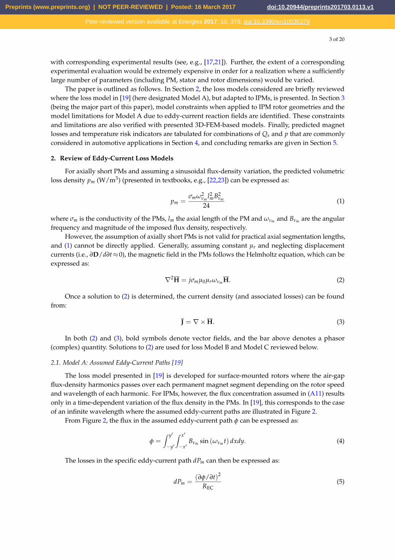
A three-phase IPM with Qs =12 slots and p=8 poles with additional key parameters reported inTable A1 in Appendix B is used initially for evaluation. The machine geometry is depicted in Figure 5a;the PM width is wm =15 mm, and the axial length of the PM is varied so that lm =10, 30 and 100 mm,respectively. The rotor speed is varied up to 9000 rpm.
A brief review of the fundamentals of the resulting harmonic content is provided in Appendix A.From (A1), the winding periodicity is found as tper = 4. Therefore, from (A4), the harmonic ordersthat could be present in the air gap due to the armature reaction (assuming sinusoidal phase currents)are ν = 4, 8, 12, 16, 20, . . .. However, from (A6), kν = 0 for harmonics that are multiples of 12. Themagnitude of the corresponding harmonics can be obtained using (A3)–(A9). Hence, in the air gap, thethree first harmonic orders are ν=4, 8 and 16. For the considered rotor structures, αp≈0.77 and using(A5) and (A12), the first harmonic order present in a PM is νm =12 (higher order harmonics exist, but
Preprints (www.preprints.org) | NOT PEER-REVIEWED | Posted: 16 March 2017 doi:10.20944/preprints201703.0113.v1
Peer-reviewed version available at Energies 2017, 10, 379; doi:10.3390/en10030379
9 of 20
are of significantly lower magnitude and contribute only minorly to the total eddy-current losses).Hence, at 9000 rpm, ωνm /(2π)=12 · 9000/60=1800 Hz.
Version February 26, 2017 submitted to Energies 9 of 20
(a) (b)
(c)
Figure 5. IPM 3D-FEM models: (a) V-shaped interior PMs (wm = 15 mm); (b) V-shaped interior PMs
(wm=30 mm); (c) Straight interior PMs (wm =40 mm).
could be present in the air gap due to the armature reaction (assuming sinusoidal phase currents)148
are ν = 4, 8, 12, 16, 20, . . .. However, from (34), kν = 0 for harmonics that are multiples of 12. The149
magnitude of the corresponding harmonics can be obtained using (31)–(37). Hence, in the air gap,150
the three first harmonic orders are ν= 4, 8, and 16. For the considered rotor structures, αp ≈ 0.77 and151
using (33) and (40), the first harmonic order present in a PM is νm =12 (higher order harmonics exist152
but are of significantly lower magnitude and contribute only minor to the total eddy-current losses).153
Hence, at 9000 rpm, ωνm/(2π)=12 · 9000/60=1800 Hz.154
Remark: Since the PMs are mounted in the interior of the rotor, the resulting eddy-current losses155
due to the slot-opening effect is negligible compared to the eddy-current losses due to the armature156
reaction.157
3.3.1. Negligible Eddy-Current Reaction Fields158
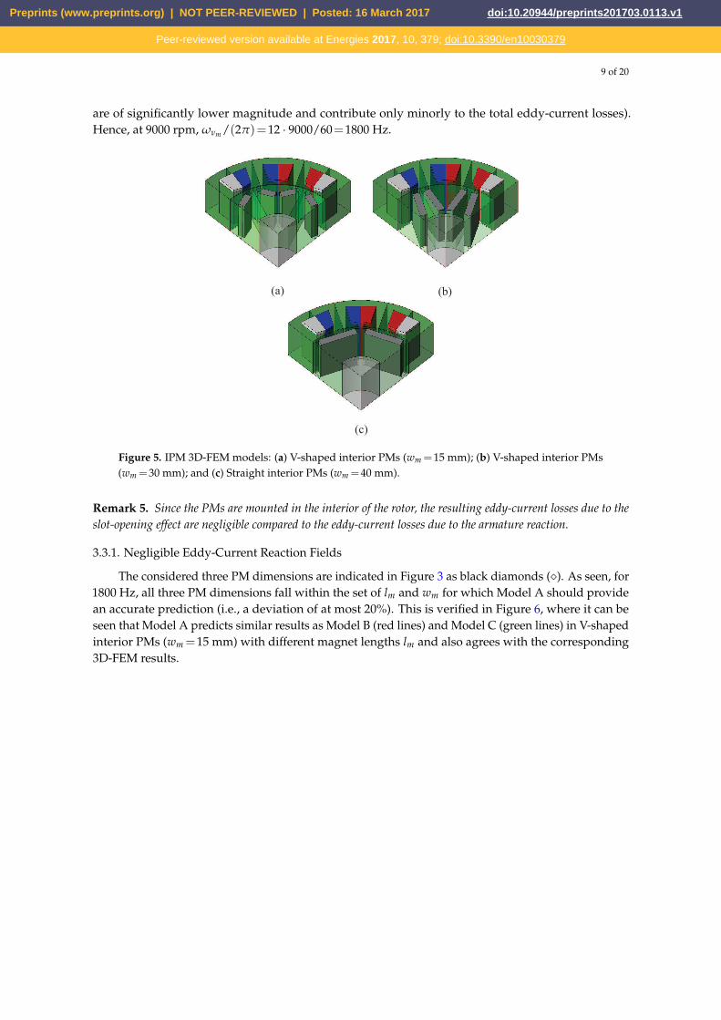
The considered three PM dimensions are indicated in Figure 3 as black diamonds (⋄). As seen,159
for 1800 Hz, all three PM dimensions fall within the set of lm and wm for which Model A should160
provide an accurate prediction (i.e., a deviation of at most 20 %). This is verified in Figure 6 where161
it can be seen that Model A predicts similar results as Model B (red lines) and Model C (green lines)162
in V-shaped interior PMs (wm = 15 mm) with different magnet lengths lm, and also agrees with the163
corresponding 3D-FEM results.164
3.3.2. Non-Negligible Eddy-Current Reaction Fields165
With a wider magnet width wm =30 mm (see Figure 5 (b)), it can be seen from Figure 3 (depicted166
as a blue circle (◦)) that Model A will overestimate the eddy-current losses for frequencies above167
around 1700 Hz (corresponding to rotor speeds around 8500 rpm). This is verified in Figure 7168
where the losses are substantially overestimated at speeds above (around) 8500 rpm. Compensating169
Model A as Pm/(
εA|B + 1)
using the approximation of εA|B given by (26) yields a significantly better170
agreement with the corresponding 3D-FEM results. Model B and Model C predict similar results,171
both agreeing well the corresponding 3D-FEM results at all rotor speeds considered.172
Figure 5. IPM 3D-FEM models: (a) V-shaped interior PMs (wm =15 mm); (b) V-shaped interior PMs(wm =30 mm); and (c) Straight interior PMs (wm =40 mm).
Remark 5. Since the PMs are mounted in the interior of the rotor, the resulting eddy-current losses due to theslot-opening effect are negligible compared to the eddy-current losses due to the armature reaction.
3.3.1. Negligible Eddy-Current Reaction Fields
The considered three PM dimensions are indicated in Figure 3 as black diamonds (�). As seen, for1800 Hz, all three PM dimensions fall within the set of lm and wm for which Model A should providean accurate prediction (i.e., a deviation of at most 20%). This is verified in Figure 6, where it can beseen that Model A predicts similar results as Model B (red lines) and Model C (green lines) in V-shapedinterior PMs (wm =15 mm) with different magnet lengths lm and also agrees with the corresponding3D-FEM results.
Preprints (www.preprints.org) | NOT PEER-REVIEWED | Posted: 16 March 2017 doi:10.20944/preprints201703.0113.v1
Peer-reviewed version available at Energies 2017, 10, 379; doi:10.3390/en10030379

10 of 20Version February 26, 2017 submitted to Energies 10 of 20
0 2000 4000 6000 8000 100000
0.2
0.4
0 2000 4000 6000 8000 100000
2
4
0 2000 4000 6000 8000 100000
5
10
15
(a)
(b)
(c)
Lo
ss(W
)L
oss
(W)
Lo
ss(W
)
Speed (rpm)
Figure 6. Predicted losses per magnet segment Pm as function of rotor speed and for different magnet
lengths lm in V-shaped interior PMs (wm=15 mm) for Model A (blue line), Model B (red line), Model C
(green line), and corresponding 3D-FEM results (diamonds “⋄"): (a) lm = 10 mm; (b) lm = 30 mm; (c)
lm=100 mm.
Remark: Since the PMs are buried very deep into the rotor structure, (39) represents an overly173
simplistic approach for predicting the flux-density variation (while still being relatively uniform).174
Therefore, for this case only, the actual flux density Bm(θr) is extracted from static 2D-FEM models.175
3.3.3. Impact of Non-Uniform Flux-Density Variation176
Following the discussion in Section 3.1, the magnet width wm for the straight IPM depicted in177
Figure 5 (c) (PM dimensions marked as the red square (�) in Figure 3) is wider than half of the178
dominant harmonic’s wavelength λν. Therefore, the flux-density variation is not uniform and the179
loss prediction accuracy for all three models worsens. This is verified in Figure 8 where neither of the180
models are in agreement with the corresponding 3D-FEM results.181
3.4. Visualization of Resulting Eddy-Current Distribution182
As is well known, the time-dependent currents densities found from the time-harmonic
(complex) formulations used in Model B and Model C can be determined as
Jx(t) = ℜ {Jx
}cos (ωνmt)−ℑ {
Jx
}sin (ωνmt) (27)
Jy(t) = ℜ{
Jy
}cos (ωνmt)−ℑ
{Jy
}sin (ωνmt) . (28)
Figure 9 shows the resulting eddy-current distributions in a PM segment of the IPM depicted in183
Figure 5 (b) for two different speeds (1000 and 15000 rpm) with a PM segment length lm = 60 mm.184
Figure 6. Predicted losses per magnet segment Pm as a function of rotor speed and for different magnetlengths lm in V-shaped interior PMs (wm =15 mm) for Model A (blue line), Model B (red line), Model C(green line) and corresponding 3D-FEM results (diamonds “�"): (a) lm =10 mm; (b) lm =30 mm; and(c) lm =100 mm.
3.3.2. Non-Negligible Eddy-Current Reaction Fields
With a wider magnet width wm =30 mm (see Figure 5b), it can be seen from Figure 3 (depicted asa blue circle (◦)) that Model A will overestimate the eddy-current losses for frequencies above around1700 Hz (corresponding to rotor speeds around 8500 rpm). This is verified in Figure 7 where thelosses are substantially overestimated at speeds above (around) 8500 rpm. Compensating Model A asPm/
(εA|B + 1
)using the approximation of εA|B given by (26) yields a significantly better agreement
with the corresponding 3D-FEM results. Model B and Model C predict similar results, both agreeingwell with the corresponding 3D-FEM results at all rotor speeds considered.Version February 26, 2017 submitted to Energies 11 of 20
0 5000 10000 150000
50
100
150
Lo
ss(W
)
Speed (rpm)
Figure 7. Predicted losses per magnet segment Pm as function of rotor speed and for magnet lengths
lm = 60 mm in V-shaped interior PMs (wm = 30 mm) for Model A (blue lines), Model A but
compensated as Pm/(εA|B + 1) (dashed blue line), Model B (red line), Model C (green line), and
corresponding 3D-FEM results (circles “◦").
0 5000 10000 150000
100
200
300
400
Lo
ss(W
)
Speed (rpm)
Figure 8. Predicted losses per magnet segment Pm as function of rotor speed for lm = 60 mm for
the straight IPM depicted in Figure 5 (c)s (wm = 40 mm) for Model A (blue line), Model B (red line),
Model C (green line), and corresponding 3D-FEM results (squares “�").
Predicted distributions using Model B (red contours) and Model C (green contours). First, it is185
noted that the resulting eddy-current distributions predicted by the two models are essentially186
equal. Hence, both models can be expected to predict similar eddy-current losses. Further, at187
1000 rpm, the eddy current distribution is very similar to what is assumed in Model A (compare188
with Figure 2). However, at higher speeds, the eddy current paths during the transition between189
“clockwise" and “anti-clockwise" current paths becomes more complex with additional eddies close190
to corners. Corresponding 3D-FEM results are depicted in Figure 10 and, as seen, the eddy-current191
distributions predicted with Model B and Model C are in good agreement with the 3D-FEM results.192
In Figure 11, the predicted current densities |J|=√
J2x + J2
y at 15000 rpm in selected positions ’Pa’193
and ’Pb’ (see Figure 9 (b)) using Model A, Model B, Model C, and corresponding 3D-FEM results are194
reported. As seen, Model B and Model C are agreeing well with the 3D-FEM based results whereas195
Model A overestimates the eddy-currents significantly.196
4. PM Losses Automotive Applications197
4.1. Thermal Impact198
While Figure 3 or its approximation (26) provide necessary input on which loss model is suitable,199
the associated temperature increase in the PMs (due to the eddy currents) represents a key limiting200
factor for the machine designer. To investigate this thermal impact, a set of 3D-FEM thermal201
simulations of the machine described above are carried out at 9000 rpm and rated current for different202
volumetric loss densities pm in the PMs. The implemented thermal model is similar to the 3D-FEM203
Figure 7. Predicted losses per magnet segment Pm as a function of rotor speed and for magnetlengths lm = 60 mm in V-shaped interior PMs (wm = 30 mm) for Model A (blue lines), Model A,but compensated as Pm/(εA|B + 1) (dashed blue line), Model B (red line), Model C (green line) andcorresponding 3D-FEM results (circles “◦").
Preprints (www.preprints.org) | NOT PEER-REVIEWED | Posted: 16 March 2017 doi:10.20944/preprints201703.0113.v1
Peer-reviewed version available at Energies 2017, 10, 379; doi:10.3390/en10030379

11 of 20
Remark 6. Since the PMs are buried very deep into the rotor structure, (A11) represents an overly simplisticapproach for predicting the flux-density variation (while still being relatively uniform). Therefore, for this caseonly, the actual flux density Bm(θr) is extracted from static 2D-FEM models.
3.3.3. Impact of Non-Uniform Flux-Density Variation
Following the discussion in Section 3.1, the magnet width wm for the straight IPM depicted inFigure 5c (PM dimensions marked as the red square (�) in Figure 3) is wider than half of the dominantharmonic’s wavelength λν. Therefore, the flux-density variation is not uniform, and the loss predictionaccuracy for all three models worsens. This is verified in Figure 8 where neither of the models are inagreement with the corresponding 3D-FEM results.
Version February 26, 2017 submitted to Energies 11 of 20
0 5000 10000 150000
50
100
150
Lo
ss(W
)
Speed (rpm)
Figure 7. Predicted losses per magnet segment Pm as function of rotor speed and for magnet lengths
lm = 60 mm in V-shaped interior PMs (wm = 30 mm) for Model A (blue lines), Model A but
compensated as Pm/(εA|B + 1) (dashed blue line), Model B (red line), Model C (green line), and
corresponding 3D-FEM results (circles “◦").
0 5000 10000 150000
100
200
300
400
Lo
ss(W
)
Speed (rpm)
Figure 8. Predicted losses per magnet segment Pm as function of rotor speed for lm = 60 mm for
the straight IPM depicted in Figure 5 (c)s (wm = 40 mm) for Model A (blue line), Model B (red line),
Model C (green line), and corresponding 3D-FEM results (squares “�").
Predicted distributions using Model B (red contours) and Model C (green contours). First, it is185
noted that the resulting eddy-current distributions predicted by the two models are essentially186
equal. Hence, both models can be expected to predict similar eddy-current losses. Further, at187
1000 rpm, the eddy current distribution is very similar to what is assumed in Model A (compare188
with Figure 2). However, at higher speeds, the eddy current paths during the transition between189
“clockwise" and “anti-clockwise" current paths becomes more complex with additional eddies close190
to corners. Corresponding 3D-FEM results are depicted in Figure 10 and, as seen, the eddy-current191
distributions predicted with Model B and Model C are in good agreement with the 3D-FEM results.192
In Figure 11, the predicted current densities |J|=√
J2x + J2
y at 15000 rpm in selected positions ’Pa’193
and ’Pb’ (see Figure 9 (b)) using Model A, Model B, Model C, and corresponding 3D-FEM results are194
reported. As seen, Model B and Model C are agreeing well with the 3D-FEM based results whereas195
Model A overestimates the eddy-currents significantly.196
4. PM Losses Automotive Applications197
4.1. Thermal Impact198
While Figure 3 or its approximation (26) provide necessary input on which loss model is suitable,199
the associated temperature increase in the PMs (due to the eddy currents) represents a key limiting200
factor for the machine designer. To investigate this thermal impact, a set of 3D-FEM thermal201
simulations of the machine described above are carried out at 9000 rpm and rated current for different202
volumetric loss densities pm in the PMs. The implemented thermal model is similar to the 3D-FEM203
Figure 8. Predicted losses per magnet segment Pm as a function of rotor speed for lm = 60 mm forthe straight IPM depicted in Figure 5 (c)s (wm = 40 mm) for Model A (blue line), Model B (red line),Model C (green line) and corresponding 3D-FEM results (squares “�").
3.4. Visualization of the Resulting Eddy-Current Distribution
As is well known, the time-dependent currents densities found from the time-harmonic (complex)formulations used in Model B and Model C can be determined as:
Jx(t) = <{
Jx}
cos (ωνm t)−={
Jx}
sin (ωνm t) (27)
Jy(t) = <{
Jy
}cos (ωνm t)−=
{Jy
}sin (ωνm t) . (28)
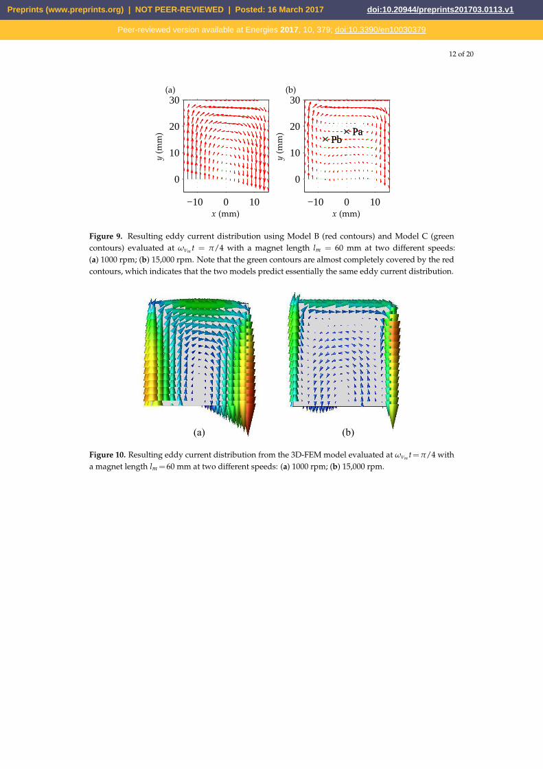
Figure 9 shows the resulting eddy-current distributions in a PM segment of the IPM depictedin Figure 5b for two different speeds (1000 and 15,000 rpm) with a PM segment length lm =60 mm;predicted distributions using Model B (red contours) and Model C (green contours). First, it is notedthat the resulting eddy-current distributions predicted by the two models are essentially equal. Hence,both models can be expected to predict similar eddy-current losses. Further, at 1000 rpm, the eddycurrent distribution is very similar to what is assumed in Model A (compare with Figure 2). However,at higher speeds, the eddy current paths during the transition between “clockwise” and “anti-clockwise”current paths becomes more complex with additional eddies close to corners. Corresponding 3D-FEMresults are depicted in Figure 10, and as seen, the eddy-current distributions predicted with Model Band Model C are in good agreement with the 3D-FEM results.
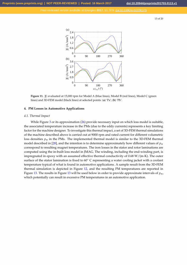
In Figure 11, the predicted current densities |J|=√
J2x + J2
y at 15, 000 rpm in selected positions ‘Pa’and ‘Pb’ (see Figure 9b) using Model A, Model B, Model C and the corresponding 3D-FEM results arereported. As seen, Model B and Model C are agreeing well with the 3D-FEM based results, whereasModel A overestimates the eddy-currents significantly.
Preprints (www.preprints.org) | NOT PEER-REVIEWED | Posted: 16 March 2017 doi:10.20944/preprints201703.0113.v1
Peer-reviewed version available at Energies 2017, 10, 379; doi:10.3390/en10030379
12 of 20Version February 26, 2017 submitted to Energies 12 of 20
−10 0 10
0
10
20
30
−10 0 10
0
10
20
30
PaPb
PaPb
(a) (b)
x (mm)x (mm)
y(m
m)
y(m
m)
Figure 9. Resulting eddy current distribution using Model B (red contours) and Model C (green
contours) evaluated at ωνm t = π/4 with a magnet length lm = 60 mm at two different speeds: (a)
1000 rpm; (b) 15000 rpm. Note that the green contours are almost completely covered by the red
contours which indicates that the two models predict essentially the same eddy current distribution.
(a) (b)
Figure 10. Resulting eddy current distribution from the 3D-FEM model evaluated at ωνm t=π/4 with
a magnet length lm =60 mm at two different speeds: (a) 1000 rpm; (b) 15000 rpm.
thermal model described in [28] and the intention is to determine approximately how different values204
of pm correspond to resulting magnet temperatures. The iron losses in the stator and rotor laminations205
are computed using the in-built loss model in JMAG. The winding, including the end-winding part,206
is impregnated in Epoxy with an assumed effective thermal conductivity of 0.68 W/(m·K). The207
outer surface of the stator lamination is fixed to 60◦ C representing a water cooling jacket with a208
coolant temperature typical to what found in automotive applications. A sample result from the209
3D-FEM thermal simulation is depicted in Figure 12 and the resulting PM temperatures are reported210
in Figure 13. The results in Figure 13 will be used below in order to provide approximate intervals of211
pm which potentially can result in excessive PM temperatures in an automotive application.212
4.2. Losses for p and Qs Common in Automotive Applications213
Now, resulting PM eddy-current losses for combinations of p and Qs often considered in214
automotive applications are considered. The harmonic content from double-layer FSCWs are215
considered in this paper. For single-layer FSCWs, the harmonic content is described in [8,12,14]. The216
rotor radius rr and air-gap length δ are selected identical to what reported in Table B.1 and the main217
harmonic stator MMF (the ampere-turns and winding factor kν=p/2 product) is also kept the same218
Figure 9. Resulting eddy current distribution using Model B (red contours) and Model C (greencontours) evaluated at ωνm t = π/4 with a magnet length lm = 60 mm at two different speeds:(a) 1000 rpm; (b) 15,000 rpm. Note that the green contours are almost completely covered by the redcontours, which indicates that the two models predict essentially the same eddy current distribution.
Version February 26, 2017 submitted to Energies 12 of 20
−10 0 10
0
10
20
30
−10 0 10
0
10
20
30
PaPb
PaPb
(a) (b)
x (mm)x (mm)
y(m
m)
y(m
m)
Figure 9. Resulting eddy current distribution using Model B (red contours) and Model C (green
contours) evaluated at ωνm t = π/4 with a magnet length lm = 60 mm at two different speeds: (a)
1000 rpm; (b) 15000 rpm. Note that the green contours are almost completely covered by the red
contours which indicates that the two models predict essentially the same eddy current distribution.
(a) (b)
Figure 10. Resulting eddy current distribution from the 3D-FEM model evaluated at ωνm t=π/4 with
a magnet length lm =60 mm at two different speeds: (a) 1000 rpm; (b) 15000 rpm.
thermal model described in [28] and the intention is to determine approximately how different values204
of pm correspond to resulting magnet temperatures. The iron losses in the stator and rotor laminations205
are computed using the in-built loss model in JMAG. The winding, including the end-winding part,206
is impregnated in Epoxy with an assumed effective thermal conductivity of 0.68 W/(m·K). The207
outer surface of the stator lamination is fixed to 60◦ C representing a water cooling jacket with a208
coolant temperature typical to what found in automotive applications. A sample result from the209
3D-FEM thermal simulation is depicted in Figure 12 and the resulting PM temperatures are reported210
in Figure 13. The results in Figure 13 will be used below in order to provide approximate intervals of211
pm which potentially can result in excessive PM temperatures in an automotive application.212
4.2. Losses for p and Qs Common in Automotive Applications213
Now, resulting PM eddy-current losses for combinations of p and Qs often considered in214
automotive applications are considered. The harmonic content from double-layer FSCWs are215
considered in this paper. For single-layer FSCWs, the harmonic content is described in [8,12,14]. The216
rotor radius rr and air-gap length δ are selected identical to what reported in Table B.1 and the main217
harmonic stator MMF (the ampere-turns and winding factor kν=p/2 product) is also kept the same218
Figure 10. Resulting eddy current distribution from the 3D-FEM model evaluated at ωνm t=π/4 witha magnet length lm =60 mm at two different speeds: (a) 1000 rpm; (b) 15,000 rpm.
Preprints (www.preprints.org) | NOT PEER-REVIEWED | Posted: 16 March 2017 doi:10.20944/preprints201703.0113.v1
Peer-reviewed version available at Energies 2017, 10, 379; doi:10.3390/en10030379
13 of 20Version February 26, 2017 submitted to Energies 13 of 20
0 90 180 270 3600
0.6
1.2
1.8
2.4
0 90 180 270 3600
0.9
1.8
2.7
3.6
(a)
(b)
|J|(A
/m
m2)
|J|(A
/m
m2)
ωνmt (o)
Figure 11. |J| evaluated at 15000 rpm for Model A (blue lines), Model B (red lines), Model C (green
lines), and 3D-FEM model (black lines) at selected points: (a) ’Pa’; (b) ’Pb’.
meaning that each resulting machine design results in a similar output torque (the harmonic content219
will be different, however, for each combination of p and Qs). The pole-cap coefficient is selected to220
αp =3/4 to yield a rotor saliency and the PM height is selected to hm =5 mm. Further, the PM width221
wm is selected so that the no-load flux density in the air gap is 0.75 T. For p = 8, 10, 12, and 14, this222
results in wm = 14.2, 11.3, 9.5, and 8.1 mm. Resulting rotor geometries for p = 8 and p = 14 (with223
magnetic bridges and air pockets inserted) are depicted in Figure 14.224
The resulting PM loss densities for lm = 10 mm and lm = 30 mm are reported in Table 1225
and Table 2, respectively. As seen, only a few combinations of p and Qs result in sufficiently low226
eddy-current losses so that excessive PM temperatures are avoided. Also, the increase of PM length227
from lm = 10 mm to lm = 30 mm rules out all but two combinations of p and Qs. Further, the loss228
densities reported in Table 1 and Table 2 are predictions using Model C. However, using Figure 3 or229
its approximation (26), it can be determined that Model A provides sufficient accuracy (i.e., within a230
20% deviation from Model B and Model C) for all cases considered in Table 1 and Table 2.
Table 1. pm [W/cm3] for lm=10 mm at 9000 rpm
Qs \p 8 10 12 14
6 4.0 4.7 N.F. 4.19 N.F. N.F. 6.3 N.F.
12 0.8 2.0 N.F. 6.2
15 N.F. 1.0 N.F. N.F.18 0.5 0.5 1.2 4.6
21 N.F N.F. N.F. 1.3
24 qs =1 5.6 N.F. 7.727 N.F. 0.8 N.F.
30 qs =1 N.F. 0.9
N.F. Not feasible/unbalanced windingDistributed windings
Low lossesMedium losses
High losses
Figure 11. |J| evaluated at 15,000 rpm for Model A (blue lines), Model B (red lines), Model C (greenlines) and 3D-FEM model (black lines) at selected points: (a) ‘Pa’; (b) ‘Pb’.
4. PM Losses in Automotive Applications
4.1. Thermal Impact
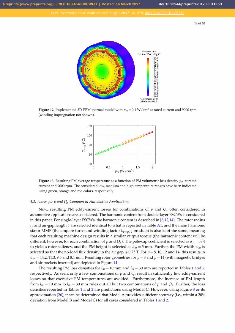
While Figure 3 or its approximation (26) provide necessary input on which loss model is suitable,the associated temperature increase in the PMs (due to the eddy currents) represents a key limitingfactor for the machine designer. To investigate this thermal impact, a set of 3D-FEM thermal simulationsof the machine described above is carried out at 9000 rpm and rated current for different volumetricloss densities pm in the PMs. The implemented thermal model is similar to the 3D-FEM thermalmodel described in [28], and the intention is to determine approximately how different values of pm
correspond to resulting magnet temperatures. The iron losses in the stator and rotor laminations arecomputed using the in-built loss model in JMAG. The winding, including the end-winding part, isimpregnated in epoxy with an assumed effective thermal conductivity of 0.68 W/(m·K). The outersurface of the stator lamination is fixed to 60◦ C representing a water cooling jacket with a coolanttemperature typical of what is found in automotive applications. A sample result from the 3D-FEMthermal simulation is depicted in Figure 12, and the resulting PM temperatures are reported inFigure 13. The results in Figure 13 will be used below in order to provide approximate intervals of pm,which potentially can result in excessive PM temperatures in an automotive application.
Preprints (www.preprints.org) | NOT PEER-REVIEWED | Posted: 16 March 2017 doi:10.20944/preprints201703.0113.v1
Peer-reviewed version available at Energies 2017, 10, 379; doi:10.3390/en10030379
14 of 20
Figure 12. Implemented 3D-FEM thermal model with pm =0.1 W/cm3 at rated current and 9000 rpm(winding impregnation not shown).
Version February 26, 2017 submitted to Energies 14 of 20
Figure 12. Implemented 3D-FEM thermal model with pm =0.1 W/cm3 at rated current and 9000 rpm
(winding impregnation not shown).
0 0.5 1 1.5 260
90
120
150
180
pm (W/cm3)
Tm
ag
(oC
)
Figure 13. Resulting PM average temperature as function of PM volumetric loss density pm at rated
current and 9000 rpm. The considered low, medium and high temperature ranges have been indicated
using green, orange and red colors, respectively.
5. Conclusions231
In this paper, three models for predicting average magnet losses in IPMs with FSCWs due to232
induced eddy currents caused by the armature reaction (assuming sinusoidal phase currents) were233
analyzed and compared. Provided that the harmonic order ν that dominates the PM losses is less234
or equal to to the number of poles p, it was found that that for V-shaped PMs, a uniform flux235
density variation in the PMs can typically be assumed. Boundaries in terms of PM dimensions236
and angular frequency were identified to aid the machine designer whether the simplest loss model237
(Model A) is applicable or not. An approximate analytical expression to these boundaries was also238
identified. It was found that Model B and Model C, while relying on different formulations and239
solutions of Helmholtz equation, provide very similar loss predictions in very good agreement with240
corresponding 3D-FEM based simulations. Further, tables were provided with resulting volumetric241
loss densities pm for combinations of Qs and p commonly used in automotive applications. Finally, by242
compiling results from previous publications, a complete description on how to analytically predict243
the magnitudes Bνm and corresponding harmonic orders νm for FSCW-IPMs was provided in the244
appendix.245
Figure 13. Resulting PM average temperature as a function of PM volumetric loss density pm at ratedcurrent and 9000 rpm. The considered low, medium and high temperature ranges have been indicatedusing green, orange and red colors, respectively.
4.2. Losses for p and Qs Common in Automotive Applications
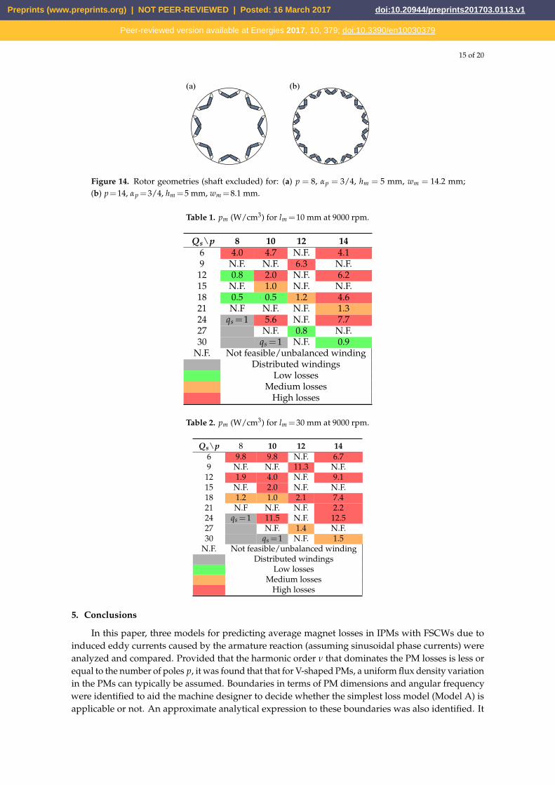
Now, resulting PM eddy-current losses for combinations of p and Qs often considered inautomotive applications are considered. The harmonic content from double-layer FSCWs is consideredin this paper. For single-layer FSCWs, the harmonic content is described in [8,12,14]. The rotor radiusrr and air-gap length δ are selected identical to what is reported in Table A1, and the main harmonicstator MMF (the ampere-turns and winding factor kν=p/2 product) is also kept the same, meaningthat each resulting machine design results in a similar output torque (the harmonic content will bedifferent, however, for each combination of p and Qs). The pole-cap coefficient is selected as αp =3/4to yield a rotor saliency, and the PM height is selected as hm = 5 mm. Further, the PM width wm isselected so that the no-load flux density in the air gap is 0.75 T. For p=8, 10, 12 and 14, this results inwm =14.2, 11.3, 9.5 and 8.1 mm. Resulting rotor geometries for p=8 and p=14 (with magnetic bridgesand air pockets inserted) are depicted in Figure 14.
The resulting PM loss densities for lm = 10 mm and lm = 30 mm are reported in Tables 1 and 2,respectively. As seen, only a few combinations of p and Qs result in sufficiently low eddy-currentlosses so that excessive PM temperatures are avoided. Furthermore, the increase of PM lengthfrom lm = 10 mm to lm = 30 mm rules out all but two combinations of p and Qs. Further, the lossdensities reported in Tables 1 and 2 are predictions using Model C. However, using Figure 3 or itsapproximation (26), it can be determined that Model A provides sufficient accuracy (i.e., within a 20%deviation from Model B and Model C) for all cases considered in Tables 1 and 2.
Preprints (www.preprints.org) | NOT PEER-REVIEWED | Posted: 16 March 2017 doi:10.20944/preprints201703.0113.v1
Peer-reviewed version available at Energies 2017, 10, 379; doi:10.3390/en10030379
15 of 20Version February 26, 2017 submitted to Energies 15 of 20
Figure 14. Rotor geometries (shaft excluded) for (a) p = 8, αp = 3/4, hm = 5 mm, wm = 14.2 mm;
(b) p=14, αp =3/4, hm =5 mm, wm =8.1 mm.
Table 2. pm [W/cm3] for lm=30 mm at 9000 rpm
Qs \p 8 10 12 14
6 9.8 9.8 N.F. 6.79 N.F. N.F. 11.3 N.F.
12 1.9 4.0 N.F. 9.1
15 N.F. 2.0 N.F. N.F.18 1.2 1.0 2.1 7.4
21 N.F N.F. N.F. 2.2
24 qs =1 11.5 N.F. 12.527 N.F. 1.4 N.F.
30 qs =1 N.F. 1.5
N.F. Not feasible/unbalanced windingDistributed windings
Low lossesMedium losses
High losses
Acknowledgments: The financial support from the Swedish Hybrid Vehicle Center (SHC) and the STandUP for246
Energy research initiative is gratefully acknowledged.247
Author Contributions: This paper is a result of the full collaboration of all the authors. Hui Zhang and Oskar248
Wallmark have contributed developing ideas and analytical model. Hui Zhang built the FEM models and249
analyzed the data. Oskar Wallmark was responsible for the guidance and a number of key suggestions.250
Conflicts of Interest: The authors declare no conflict of interest.251
Appendix A. FSCW Fundamentals252
How to predict the magnitudes Bνm and corresponding harmonic orders νm in FSCW-IPMs253
(compiling results from [8,10,29,30]) is, for completeness, described in this appendix.254
Appendix A.1. Preliminaries255
The winding periodicity tper can be expressed as [8]:
tper = gcd (Qs, p/2) (29)
where Qs is the number of stator slots, p the number of poles, and gcd(a, b) denotes the greatest
common denominator for a and b. Introducing mph as the (odd) number of phases, the (sinusoidal)
current in in phase n, n=1, 2, . . . , mph, can be expressed as
in =√
2I cos[ p
2
(θr − αph(n − 1)− ϕ
)]. (30)
Here, θr is the (mechanical) rotor position, ϕ is the current phase angle angle, and αph the angular256
displacement of the air-gap MMF distribution due to each adjacent phase (αph=2π/(mphtper)).257
Figure 14. Rotor geometries (shaft excluded) for: (a) p = 8, αp = 3/4, hm = 5 mm, wm = 14.2 mm;(b) p=14, αp =3/4, hm =5 mm, wm =8.1 mm.
Table 1. pm (W/cm3) for lm =10 mm at 9000 rpm.
Qs\p 8 10 12 146 4.0 4.7 N.F. 4.19 N.F. N.F. 6.3 N.F.12 0.8 2.0 N.F. 6.215 N.F. 1.0 N.F. N.F.18 0.5 0.5 1.2 4.621 N.F N.F. N.F. 1.324 qs =1 5.6 N.F. 7.727 N.F. 0.8 N.F.30 qs =1 N.F. 0.9
N.F. Not feasible/unbalanced windingDistributed windings
Low lossesMedium losses
High losses
Table 2. pm (W/cm3) for lm =30 mm at 9000 rpm.
Qs\p 8 10 12 146 9.8 9.8 N.F. 6.79 N.F. N.F. 11.3 N.F.
12 1.9 4.0 N.F. 9.115 N.F. 2.0 N.F. N.F.18 1.2 1.0 2.1 7.421 N.F N.F. N.F. 2.224 qs =1 11.5 N.F. 12.527 N.F. 1.4 N.F.30 qs =1 N.F. 1.5
N.F. Not feasible/unbalanced windingDistributed windings
Low lossesMedium losses
High losses
5. Conclusions
In this paper, three models for predicting average magnet losses in IPMs with FSCWs due toinduced eddy currents caused by the armature reaction (assuming sinusoidal phase currents) wereanalyzed and compared. Provided that the harmonic order ν that dominates the PM losses is less orequal to the number of poles p, it was found that that for V-shaped PMs, a uniform flux density variationin the PMs can typically be assumed. Boundaries in terms of PM dimensions and angular frequencywere identified to aid the machine designer to decide whether the simplest loss model (Model A) isapplicable or not. An approximate analytical expression to these boundaries was also identified. It
Preprints (www.preprints.org) | NOT PEER-REVIEWED | Posted: 16 March 2017 doi:10.20944/preprints201703.0113.v1
Peer-reviewed version available at Energies 2017, 10, 379; doi:10.3390/en10030379

16 of 20
was found that Model B and Model C, while relying on different formulations and solutions of theHelmholtz equation, provide very similar loss predictions in very good agreement with corresponding3D-FEM-based simulations. Further, tables were provided with resulting volumetric loss densities pm
for combinations of Qs and p commonly used in automotive applications. Finally, by compiling resultsfrom previous publications, a complete description on how to analytically predict the magnitudes Bνm
and corresponding harmonic orders νm for FSCW-IPMs was provided in the Appendix.
Acknowledgments: The financial support from the Swedish Hybrid Vehicle Center (SHC) and the STandUP forEnergy research initiative is gratefully acknowledged.
Author Contributions: This paper is a result of the full collaboration of all of the authors. Hui Zhang andOskar Wallmark have contributed by developing ideas and the analytical model. Hui Zhang built the FEM modelsand analyzed the data. Oskar Wallmark was responsible for the guidance and a number of key suggestions.
Conflicts of Interest: The authors declare no conflict of interest.
Appendix A. FSCW Fundamentals
How to predict the magnitudes Bνm and corresponding harmonic orders νm in FSCW-IPMs(compiling results from [8,10,29,30]) is, for completeness, described in this Appendix.
Appendix A.1. Preliminaries
The winding periodicity tper can be expressed as [8]:
tper = gcd (Qs, p/2) (A1)
where Qs is the number of stator slots, p the number of poles and gcd(a, b) denotes the greatestcommon denominator for a and b. Introducing mph as the (odd) number of phases, the (sinusoidal)current in in phase n, n=1, 2, . . . , mph, can be expressed as:
in =√
2I cos[ p
2
(θr − αph(n− 1)− ϕ
)]. (A2)
Here, θr is the (mechanical) rotor position; ϕ is the current phase angle angle; and αph the angulardisplacement of the air-gap MMF distribution due to each adjacent phase (αph=2π/(mphtper)).
Appendix A.2. Air-Gap MMF Distribution Due to Stator Current
Assuming that all coils belonging to each phase are series connected, the resulting air-gap MMFFδ can be expressed as [31]:
Fδ = ∑ν
{mph
∑n=1
nsQskνin
πmphνcos
[ν(
θs − αph(n− 1))]}
(A3)
where ns is the number of turns per slot, kν the winding factor for harmonic ν and θs is an anglespanning the air-gap circumference (expressed in mechanical degrees). Equation (A3) is valid ifmagnetic saturation can be neglected, and it is derived assuming that the current in the stator slots canbe represented as point-like sources. The harmonic orders ν that can be present in the air gap can beexpressed as [8]:
ν =
{(2k− 1)tper, if Qs/tper is evenktper, if Qs/tper is odd
(A4)
where k is an integer. Now, sgn(ν) is introduced to denote the direction of rotation of each MMFharmonic ν with respect to the rotor. Following from (A3) (see [29] for further details), sgn(ν) can beexpressed as:
Preprints (www.preprints.org) | NOT PEER-REVIEWED | Posted: 16 March 2017 doi:10.20944/preprints201703.0113.v1
Peer-reviewed version available at Energies 2017, 10, 379; doi:10.3390/en10030379

17 of 20
sgn(ν) =
+1, if rem( p
2− ν, mphtper
)
−1, if rem( p
2+ ν, mphtper
) (A5)
Note that (A5) is applicable only to harmonics ν that can be present in the air gap (definedby (A4)).
Appendix A.3. Winding Factor for Harmonic ν
The winding factor for harmonic ν kν can be expressed as [8,29]:
kν =
sin( qphαph,ν
2
)sin(
πν
Qs
)
qph sin(
αph,ν
2
) , if qph is odd
sin( qphαph,ν
4
)sin(
πν
Qs
)
qph
2sin(
αph,ν
2
) , if qph is even
(A6)
where the electrical angle between the electromotive force of two adjacent coils αph and the number ofspokes per phase in the star of slot qph are given as:
αph,ν = π − 2πν
Qsround (Qs/p) (A7)
qph = Qs/(
mphtper
). (A8)
A sufficient condition for (A6) to be valid is [29]:
round (Qs/p) =
round(Qsqph
p
)
qph, if qph is odd
round(Qsqph
2p
)
qph
2
, if qph is even
(A9)
If (A9) is not fulfilled, the winding factor can then be computed by numerically computing theharmonic content of Fδ as in [10,30].
Appendix A.4. PM Flux Density Variations
The pole-cap coefficient αp defined in Figure A1 is an approximate measure of how much fluxoccurs across a complete pole pitch that is concentrated through the PMs.
Remark 7. Note that the geometries depicted in Figure A1 are simplified without the presence of eventualmagnetic bridges used to fix the PMs. This simplification will render the predicted flux-density magnitudes Bνm
approximate (mainly due to flux-leakage drop the magnetic bridges). If required, more accurate predictions ofBνm can rapidly be obtained using two-dimensional static FEM simulations.
Now, ψm(θr) (a function of the rotor position θr) is introduced to denote the flux in a PM pole dueto Fδ. From the geometries depicted in Figure A1, it follows that ψm(θr) can be approximated as:
ψm(θr) =µ0lmrr
(δ + hm)
∫ (θr+αp)π/p
(θr−αp)π/pFδdθs (A10)
Preprints (www.preprints.org) | NOT PEER-REVIEWED | Posted: 16 March 2017 doi:10.20944/preprints201703.0113.v1
Peer-reviewed version available at Energies 2017, 10, 379; doi:10.3390/en10030379

18 of 20
where µ0 is the permeability of air. The corresponding flux density in a PM Bm(θr) can now beapproximated as:
Bm(θr) =ψm(θr)
2Clmwm
=µ0rr
2(δ + hm)Cwm
∫ (θr+αp)π/p
(θr−αp)π/pFδdθs (A11)
where C=1 and C=1/2 for V-shaped and straight interior PMs, respectively. The harmonic orderspresent in Bm(θr) (of order νm and with a magnitude Bνm ) are now obtained from (A11).
Version February 26, 2017 submitted to Energies 17 of 20
A sufficient condition for (34) to be valid is [29]:
round (Qs/p) =
round
(Qsqph
p
)
qph, if qph is odd
round
(Qsqph
2p
)
qph
2
, if qph is even
(37)
If (37) is not fulfilled, the winding factor can then be computed by numerically computing the261
harmonic content of Fδ as in [10,30].262
Appendix A.4. PM Flux Density Variations263
The pole-cap coefficient αp defined in Figure A.1 is an approximate measure of how much flux264
across a complete pole pitch that is concentrated through the PMs.
Figure A.1. Magnet dimensions and definition of rotor-cap coefficient αp (note that for the coordinate
system fixed to PMs, the y-axis is directed into the paper): (a) V-shaped interior PMs; (b) Straight
interior PMs.
265
Remark: Note that the geometries depicted in Figure A.1 are simplified without the presence266
of eventual magnetic bridges used to fixate the PMs. This simplification will render the predicted267
flux-density magnitudes Bνm approximate (mainly due to flux-leakage drop the magnetic bridges). If268
required, more accurate predictions of Bνm can rapidly be obtained using two-dimensional static FEM269
simulations.270
Now, ψm(θr) (a function of the rotor position θr) is introduced to denote the flux in a PM pole
due to Fδ. From the geometries depicted in Figure A.1, it follows that ψm(θr) can be approximated as
ψm(θr) =µ0lmrr
(δ + hm)
∫ (θr+αp)π/p
(θr−αp)π/pFδdθs (38)
where µ0 is the permeability of air. The corresponding flux density in a PM Bm(θr) can now be
approximated as
Bm(θr) =ψm(θr)
2Clmwm
=µ0rr
2(δ + hm)Cwm
∫ (θr+αp)π/p
(θr−αp)π/pFδdθs (39)
Figure A1. Magnet dimensions and definition of rotor-cap coefficient αp (note that for the coordinatesystem fixed to PMs, the y-axis is directed in the paper): (a) V-shaped interior PMs; (b) straight interiorPMs.
Remark 8. Remark: When utilizing (A4) and (A5) when inserting (A3) into (A11), it can be verified that theharmonic orders present in the PMs νm can be expressed as:
νm =
{ν− p/2, if sgn(ν) = 1 and ν 6= kp/αp
ν + p/2, if sgn(ν) = −1 and ν 6= kp/αp(A12)
where k is an integer.
Appendix B. IPM Parameters
Table A1. IPM parameters.
Parameter Value Unit
# poles (p) 8 -# stator slots (Qs) 12 -
# turns per slot (ns) 16 -Rated current (I) 97 A (rms)Rotor radius (rr) 69.25 mm
Air-gap length (δ) 0.75 mmMagnet height (hm) 7.51 mm
Magnet conductivity (σm) 694 kS/mMagnet rel.perm.(µr) 1.04 -
References
Preprints (www.preprints.org) | NOT PEER-REVIEWED | Posted: 16 March 2017 doi:10.20944/preprints201703.0113.v1
Peer-reviewed version available at Energies 2017, 10, 379; doi:10.3390/en10030379

19 of 20
1. Gu, W.W.; Zhu, X.Y.; Li, Q.; Yi, D. Design and optimization of permanent magnet brushless machines forelectric vehicle applications. Energies 2015, 8, 13996–14008.
2. Lim, S.; Min, S.; Hong, J.-P. Optimal rotor design of IPM motor for improving torque performance consideringthermal demagnetization of magnet. IEEE Trans. Magn. 2015, 51, 1–5.
3. Ahn, K.; Bayrak, A.E.; Papalambros, P.Y. Electric vehicle design optimization: integration of a high-fidelityinterior-permanent-magnet motor model. IEEE Trans. Veh. Technol. 2015, 9, 3870–3877.
4. Kato, T.; Minowa, M.; Hijikata, H.; Akatsu, K.; Lorenz, R.D. Design methodology for variable leakage fluxIPM for automobile traction drives. IEEE Trans. Ind. Appl. 2015, 51, 3811–3821.
5. Wallscheid, O.; Böcker, J. Global identification of a low-order lumped-parameter thermal network forpermanent magnet synchronous motors. IEEE Trans. Energy Convers. 2016, 31, 354–365.
6. EL-Refaie, A.M.; Jahns, T.M. Application of bi-state magnetic material to an automotive IPM starter/alternator machine. IEEE Trans. Energy Convers. 2005, 20, 71–79.
7. Yang, Z.; Brown, I.P.; Krishnamurtht, M. Comparative study of interior permanent magnet, induction, andswitched reluctance motor drives for EV and HEV applications. IEEE Trans. Transport. Electrific. 2015, 1,245–254.
8. Bianchi, N.; Dai Pré, M. Use of the star of slots in designing fractional-slot single-layer synchronous motors.IET Electr. Power Appl. 2006, 153, 459–466.
9. Skaar, S.E.; Krøvel, Ø.; Nilssen, R. Distribution, Coil-span and Winding Factors for PM Machines withConcentrated Windings. In Proceedings of the International Conference on Electrical Machines (ICEM),Chania, Greece, 2–5 September 2006; p. 346.
10. Bianchi, N.; Bolognani, S.; Dai Pré, M.; Grezzani, G. Design considerations for fractional-slot windingconfigurations of synchronous machines. IEEE Trans. Ind. Appl. 2006, 42, 997–1006.
11. Aslan, B.; Semail, E.; Korecki, J.; Legranger, J. Slot/pole Combinations Choice for Concentrated MultiphaseMachines Dedicated to Mild-hybrid Applications. In Proceedings of the IEEE Industrial Electronics Society(IECON), Melbourne, Australia, 7–10 November 2011; pp. 3698–3703.
12. Bianchi, N.; Fornasiero, E. Index of rotor losses in three-phase fractional-slot permanent magnet machines.IET Electr. Power Appl. 2009, 3, 381–388.
13. Zheng, P.; Wu, F.; Lei, Y.; Sui, Y.; Yu, B. Investigation of a novel 24-slot/14-pole six-phase fault-tolerantmodular permanent-magnet in-wheel motor for electric vehicles. Energies 2013, 6, 4980–5002.
14. Bianchi, N.; Bolognani, S.; Fornasiero, E. An overview of rotor losses determination in three-phasefractional-slot PM machines. IEEE Trans. Ind. Appl. 2010, 46, 2338–2345.
15. Tangudu, J; Jahns, T. Comparison of Interior PM Machines with Concentrated and Distributed StatorWindings for Traction Applications. In Proceedings of the IEEE Vehicle Power and Propulsion Conference(VPPC), Chicago, IL, USA, 6-9 September 2011; pp. 1–8.
16. EL-Refaie, A.M.; Bolognani, S.; Fornasiero, E. Fractional-slot concentrated-windings synchronous permanentmagnet machines: opportunities and challenges. IEEE Trans. Ind. Electron. 2010, 57, 107–121.
17. Malloy, A.C.; Martinez-Botas, R.F.; Lampérth, M. Measurement of magnet losses in a surface mountedpermanent magnet synchronous machine. IEEE Trans. Energy Convers. 2015, 30, 323–330.
18. Zhang, P.; Sizov, G.Y.; He, J.; Ionel, D.M.; Demerdash, N.O.A. Calculation of magnet losses in concentratedwinding permanent magnet synchronous machines using a computationally efficient finite element method.IEEE Trans. Ind. Appl. 2013, 49, 2524–2532.
19. Aslan, B.; Semail, E.; Legranger, J. General analytical model of magnet average eddy-current volume lossesfor comparison of multiphase PM machines with concentrated winding. IEEE Trans. Energy Convers. 2014,29, 72–83.
20. Paradkar, M; Böcker, J. 3D Analytical Model for Estimation of Eddy-current Losses in the Magnets of IPMMachine Considering the Reaction Field of the Induced Eddy Currents. In Proceedings of the IEEE EnergyConversion Congress and Exposition (ECCE), Montreal, QC, Canada, 20–24 September 2015; pp. 2862–2869.
21. Yamazaki, K.; Fukushima,Y. Effect of eddy-current loss reduction by magnet segmentation in synchronousmotors with concentrated windings. IEEE Trans. Energy Convers. 2011, 47, 779–788.
22. Chalmers, B.J. Electromagnetic Problems of A.C. Machines; Chapman and Hall: London, UK, 1965; pp. 66–87.23. Sadarangani, C. Electrical Machines—Design and Analysis of Induction and Permanent Magnet Motors;
Universitetesservice: Stockholm, Sweden, 2006; pp. 543–658.
Preprints (www.preprints.org) | NOT PEER-REVIEWED | Posted: 16 March 2017 doi:10.20944/preprints201703.0113.v1
Peer-reviewed version available at Energies 2017, 10, 379; doi:10.3390/en10030379
20 of 20
24. Ruoho, S.; Santa-Nokki, T.; Kolehmainen, J.; Arkkio, A. Modeling magnet length in 2-D finite-elementanalysis of electric machines. IEEE Trans. Magn. 2009, 45, 3114–3120.
25. Krakowski, M. Eddy-current losses in thin circular and rectangular plates. Archiv für Elektrotechnik 1982, 64,307–311.
26. Sinha, G.; Prabhu, S.S. Analytical model for estimation of eddy current and power loss in conducting plateand its application. Phys. Revi. Spec. Top. Accel. Beams 2011, 14, 062401.
27. Mukerji, S.K.; George, M; Ramamurthy, M.B.; Asaduzzaman, K. Eddy currents in solid rectangular cores.Prog. Electromagn. Res. B 2008, 7, 117–131.
28. Nategh, S.; Wallmark, O.; Leksell, M.; Zhao, S. Thermal analysis of a PMaSRM using partial FEA and lumpedparameter modeling. IEEE Trans. Energy Convers. 2012, 27, 477–488.
29. Zhang, H.; Wallmark, O.; Leksell, M.; Norrga, S.; Harnefors, M.N.; Jin, L. Machine Design Considerationsfor an MHF/SPB-converter Based Electric Drive. In Proceedings of the IEEE Industrial Electronics Society(IECON), Dallas, TX, USA, 29 October–1 November 2014; pp. 3849–3854.
30. Mayer, J.; Dajaku, G.; Gerling, D. Mathematical Optimization of the MMF-function and -spectrum inConcentrated Winding Machines. In Proceedings of the International Conference on Electrical Machines andSystems (ICEMS), Beijing, China, 20–23 August 2011; pp. 1–6.
31. Zhao, L.; Li, G. The analysis of multiphase symmetrical motor winding MMF. Electr. Eng. Autom. 2013, 2,11–18.
c© 2017 by the authors. Licensee Preprints, Basel, Switzerland. This article is an open accessarticle distributed under the terms and conditions of the Creative Commons Attribution(CC-BY) license (http://creativecommons.org/licenses/by/4.0/).
Preprints (www.preprints.org) | NOT PEER-REVIEWED | Posted: 16 March 2017 doi:10.20944/preprints201703.0113.v1
Peer-reviewed version available at Energies 2017, 10, 379; doi:10.3390/en10030379

![Fractional Cascading Fractional Cascading I: A Data Structuring Technique Fractional Cascading II: Applications [Chazaelle & Guibas 1986] Dynamic Fractional.](https://static.fdocuments.us/doc/165x107/56649ea25503460f94ba64dd/fractional-cascading-fractional-cascading-i-a-data-structuring-technique-fractional.jpg)