Limit Mordell–WeilGroups and their -Adic Closure

Documenta Math. 221

Limit Mordell–Weil Groups and their p-Adic Closure

Haruzo Hida

Received: September 9, 2013

Revised: May 18, 2014

Abstract. This is a twin article of [H14b], where we study theprojective limit of the Mordell–Weil groups (called pro Λ-MW groups)of modular Jacobians of p-power level. We prove a control theorem ofan ind-version of theK-rational Λ-MW group for a number fieldK. Inaddition, we study its p-adic closure in the group of Kp-valued pointsof the modular Jacobians for a p-adic completion Kp for a prime p|pof K. As a consequence, if Kp = Qp, we give an exact formula for therank of the ordinary/co-ordinary part of the closure.

2010 Mathematics Subject Classification: primary: 11F25, 11F32,11G18, 14H40; secondary: 11D45, 11G05, 11G10Keywords and Phrases: modular curve, Hecke algebra, modular defor-mation, analytic family of modular forms, Mordell–Weil group, mod-ular jacobian

1. Introduction

Consider a p-adic ordinary family of modular eigenforms of prime-to-p levelN . This is an irreducible scheme Spec(I) which is finite torsion-free over theIwasawa algebra Zp[[T ]], and whose points P of codimension one and not inthe special fiber correspond to ordinary p-adic modular eigenforms fP . Amongthose points, many corresponds to modular classical eigenforms of weight 2 andlevel Npr (for variable r), and such points are Zariski dense in Spec(I). An old,well-known, and fundamental construction of Eichler–Shimura attaches to anymodular cuspidal eigenform f of weight 2 an abelian variety Af defined overQ, of dimension the degree of the field generated by the coefficients of f overQ. For these abelian varieties Af , one can consider the Mordell–Weil groupAf (Q) and more generally, Af (k) for k a fixed number field, which are finitely

generated abelian groups. Let us set Af (k) = Af (k) ⊗Z Zp. We consider the

following natural question: how does the Mordell–Weil group Af (k) varies asf varies among those cuspidal eigenforms of weight 2 in the family? We give apartial answer to this question in the form of control theorems (Theorems 1.1and 6.6) for these Mordell–Weil groups. An analogous result is proved when

Documenta Mathematica · Extra Volume Merkurjev (2015) 221–264

222 Haruzo Hida

the number field k is replaced by an l-adic field kl, and also a consequenceconcerning the image of Af (k) in Af (kl).

Fix a prime p. This article concerns the p-slope 0 Hecke eigen cusp forms oflevel Npr for r > 0 and p ∤ N , and for small primes p = 2, 3, they existsonly when N > 1; thus, we may assume Npr ≥ 4. Then the open curveY1(Npr) (obtained from X1(Npr) removing all cusps) gives the fine smoothmoduli scheme classifying elliptic curves E with an embedding µNpr → E.Anyway for simplicity, we assume that p ≥ 3, although we indicate often anymodification necessary for p = 2. A main difference in the case p = 2 is thatwe need to consider the level Npr with r ≥ 2, and whenever the principal ideal

(γpr−1

− 1) shows up in the statement for p > 2, we need to replace it by

(γpr−2

− 1) (assuming r ≥ 2), as the maximal torsion-free subgroup of Z×2 is

1+22Z2. We applied in [H86b] and [H14a] the techniques of U(p)-isomorphismsto p-divisible Barsotti–Tate groups of modular Jacobian varieties of all p-powerlevel (with a fixed prime-to-p level N) in order to get coherent control underdiamond operators. In this article, we apply the same techniques to Mordell–Weil groups of the Jacobians and see what we can say. We hope to studyU(p)-isomorphisms of the Tate–Shafarevich groups of the Jacobians in a futurearticle.Let Xr = X1(Npr)/Q be the compactified moduli of the classification problemof pairs (E, φ) of elliptic curves E and an embedding φ : µNpr → E[Npr] asfinite flat group schemes. Since Aut(µpr ) = (Z/prZ)×, z ∈ Z×

p acts on Xr via

φ 7→ φ z for the image z ∈ (Z/prZ)×. We write Xrs (s > r) for the quotient

curve Xs/(1 + prZp). The complex points Xrs (C) contains Γr

s\H as an openRiemann surface for Γr

s = Γ0(ps) ∩ Γ1(Npr). Write Jr/Q (resp. Jr

s/Q) for the

Jacobian of Xr (resp. Xrs ) whose origin is given by the infinity cusp ∞ of

the modular curves. We regard Jr as the degree 0 component of the Picardscheme of Xr. For a number field k, we consider the group of k-rational pointsJr(k). The Hecke operator U(p) and its dual U∗(p) act on Jr(k) and theirp-adic limit e = limn→∞ U(p)n! and e∗ = limn→∞ U∗(p)n! are well defined onthe Barsotti–Tate group Jr[p

∞]. For a general abelian variety over a number

field k, we put X(k) = X(k)⊗Z Zp (though we give the definition of the sheaf

X in the following section for global and local field k and if k is local, X maynot be the tensor product as above).

By Picard functoriality, we have injective limits J∞(k) = lim−→r

Jr(k) and

J∞[p∞](k) = lim−→r

Jr[p∞](k), on which e acts. Here Jr[p

∞] is the p-divisible

Barsotti–Tate group of Jr overQ). Write G = e(J∞[p∞]), which is called the Λ-adic Barsotti–Tate group in [H14a] and whose integral property was scrutinizedthere. We define the p-adic completion of J∞(k):

J∞(k) = lim←−n

J∞(k)/pnJ∞(k).

These groups we call ind (limit) MW-groups. Since projective limit and in-jective limit are left-exact, the functor R 7→ J∞(R) is a sheaf with values in


Limit Mordell–Weil Groups 223

abelian groups on the fppf site over Q (we call such a sheaf an fppf abeliansheaf).Adding superscript or subscript “ord” (resp. “co-ord”), we indicate the imageof e (resp. e∗). The compact cyclic group Γ = 1 + pZp ⊂ Z×

p acts on thesemodules by the diamond operators. In other words, we identify canonicallyGal(Xr/X0(Npr)) for modular curves Xr and X0(Npr) with (Z/NprZ)×, andthe group Γ acts on Jr through its image in Gal(Xr/X0(Npr)). We studycontrol of J∞(k)ord under diamond operators.A compact or discrete Zp-module M is called an Iwasawa module if it has acontinuous action of the multiplicative group Γ = 1 + pZp with a topologicalgenerator γ = 1 + p. If M is given by a projective or an injective limit ofnaturally defined compact Zp[Γ/Γ

pr

]-modules Mr, we say M has exact control

if Mr = M/(γpr

−1)M in the case of a projective limit and Mr = M [γpr

−1] =x ∈M |(γpr

− 1)x = 0 in the case of an injective limit. If M is compact andM/(γ − 1)M is finite (resp. of finite type over Zp), M is Λ-torsion (resp. of

finite type over Λ), where Λ = Zp[[Γ]] = lim←−r

Zp[Γ/Γpr

] (the Iwasawa algebra).

When p = 2, we need to take Γ = 1+ p2Z2 and γ = 1+4 = 5 ∈ Γ. In addition,we need to assume often s > r > 1 in place of s > r > 0 for odd primes.The big ordinary Hecke algebra h (whose properties we recall at the end of thissection) acts on Jord

∞ and Jord∞ as endomorphisms of functors. Let k be a number

field or a finite extension of Ql for a prime l. Write BP for Shimura’s abelianvariety quotient of Jr in [Sh73] and AP for his abelian subvariety AP ⊂ Jr[IAT, Theorem 7.14] associated to a Hecke eigenform fP in an analytic familyof slope 0 Hecke eigenforms fP |P ∈ Spec(I) (for an irreducible componentSpec(I) of Spec(h) for the big ordinary Hecke algebra h). Here we assume thatfP has weight 2 and is a p-stabilized new form of level Npr with r = r(P ) > 0.Let Spec(T) ⊂ Spec(h) be the connected component containing Spec(I). Forany h-module, we write MT (or MT) for the T-eigen component 1T · M =M ⊗h T for the idempotent 1T of T in h. Suppose that P is a principal idealgenerated by α ∈ T (regarding as P ∈ Spec(T)). This principality assumptionholds most of the cases (see Proposition 5.1). Then we may assume that α =lim←−s

αs (as an endomorphism of the fppf abelian sheaf J∞) for αs ∈ End(Js),

BP = Jr/αr(Jr), and the abelian variety AP is the connected component ofJr[αr] = Ker(αr). For a finite extension k of Q or Ql (for a prime l), we showin Section 4 that the Pontryagin dual GT(k)

∨ is often a finite module and atworst is a torsion Λ-module of finite type.In this paper as Proposition 6.4, we prove the following exact sequence:

(1.1) AP (k)ord,T ι∞−−→ J∞(k)ord,T

α−→ J∞(k)ord,T,

where Ker(ι∞) is finite and Coker(α) is a Zp-module of finite type with free

rank less than or equal to dimQp Br(k)⊗Zp Qp. The main result Theorem 6.6 of

this paper is basically the Zp-dual version of Proposition 6.4 for J∞(k)∗ord,T :=

HomZp(J∞(k)ord,T,Zp). Here is a shortened statement of our main theorem(Theorem 6.6 in the text):


224 Haruzo Hida

Theorem 1.1. The sequence Zp-dual to the one in (1.1):

(1.2) 0→ Coker(α)∗T → J∞(k)∗ord,T → J∞(k)∗ord,T → AP (k)∗ord,T → 0

is exact up to finite error.

In Theorem 6.6, we give many control sequences similar to (1.2) for otherincarnations of J∞(k)∗ord,T.

These modules J∞(k)∗ord,T are modules over the big ordinary Hecke algebra h.

We cut down these modules to an irreducible component Spec(I) of Spec(h).In other words, we study the following I-modules:

J∞(k)ordI := J∞(k)ord ⊗h I.

We could ask diverse questions out of our control theorem. For example, whenis AP (κ) dense in AP (κp) for a prime p|p of a number field κ? We can answerthis question for almost all P if κp = Qp and dimQ AP0(κ) ⊗Z Q > 0 for onesufficiently generic P0 (see Corollary 7.2). In [H14b], we extend the control

result to the projective limit lim←−r

Jr(k)ordT . In a forthcoming paper [H14c],

we prove “almost” constancy of the Mordell–Weil rank of Shimura’s abelianvariety in a p-adic analytic family.Our point is that we have a control theorem of the limit Mordell–Weil groups(under mild assumptions) which is possibly smaller than the Selmer groupsstudied more often. We hope to discuss the relation of our result to the limitSelmer group studied by Nekovar in [N06] in our future paper.The control theorems for h proven for p ≥ 5 in [H86a] and [H86b] and in[GME, Corollary 3.2.22] for general p assert that, for p > 2, the quotient

h/(γpr−1

− 1)h is canonically isomorphic to the Hecke algebra hr (r > 0) inEndZp(Jr[p

∞]ord) generated over Zp by Hecke operators T (n) (while for p = 2,

h/(γpr−2

− 1)h ∼= hr for r ≥ 2). By this control result, we showed that h is afree of finite rank over Λ (see [GK13] for the treatment for p = 2).

We recall succinctly how these control theorems were proven in [H86b] (and in[H86a]) for p ≥ 5, as it gives a good introduction to the methods used in thepresent paper. The arguments in these papers work well for p = 2, 3 assumingthat Npr ≥ 4 (see [GK13] for details in the case of p = 2). We have a wellknown commutative diagram of U(ps−r)-operators:

(1.3)

Jr,Rπ∗

−→ Jrs,R

↓ u ւ u′ ↓ u′′

Jr,Rπ∗

−→ Jrs,R,

where the middle u′ is given by Usr (p

s−r) and u and u′′ are U(ps−r). These

operators comes from the double coset Γ(

1 00 ps−r

)Γ′ for Γ = Γr

s = Γ0(ps) ∩

Γ1(Npr) and Γ′ = Γr′

s′ for suitable s ≥ r, s′ ≥ r′. Note that U(pn) = U(p)n.Then the above diagram implies

(1.4) Jr/Q[p∞]ord ∼= Jr

s/Q[p∞]ord and Jr/Q(k)

ord ∼= Jrs/Q(k)

ord.



The commutativity of the diagram (1.3) and the level lowering (1.4) are uni-versally true even when we replace the fppf abelian sheaf Jr by any fppf sheafwith reasonable U(p)-action compatible with the modular tower · · · → Xr →· · · → X1.For computational purpose, in [H86b], we identified J(C) with a subgroupof H1(Γ,T) (for the Γ-module T := R/Z with trivial Γ-action). Since

Γrs ⊲Γ1(Nps), we may consider the finite cyclic quotient group C :=

Γrs

Γ1(Nps) =

Γpr−1

/Γps−1

. By the inflation restriction sequence, we have the following com-mutative diagram with exact rows, writing H•(?,T) as H•(?):

H1(C)→

−−−−→ H1(Γrs) −−−−→ H1(Γ1(Nps))γ

pr−1=1 −−−−→ H2(C)

x ∪

xx∪

x

? −−−−→ Jrs (C) −−−−→ Js(C)[γ

pr−1

− 1] −−−−→ ?.

Since H2(C,T) = 0 and U(p)s−r(H1(C,T)) = 0, we have the control ofBarsotti–Tate groups (see [H86b] and more recent [H14a, §4–5]):

Js[p∞][γpr−1

− 1]ord/C∼= Jr[p

∞]ord/C .

Out of this control by the Γ-action of the ordinary Barsotti–Tate groupsJr[p

∞]ord, we proved the control of h (cited above) by the diamond opera-tors.A suitable power of U(p)-operator killing the kernel and cokernel of the restric-tion maps in (1) should be also universally true not just over C but over smallerrings. We will study almost the same diagram obtained by replacing H1(?,T)for ? = Γ1(Nps) and Γr

s by H1fppf(X/Q,O

×X) = PicX/Q for X = Xs and Xr

s .

In an algebro-geometric way, we verify that an appropriate power of the U(p)-operator kills the corresponding kernel and cokernel. Technical points aside,this is a key to the proof of Theorem 1.1. This principle should hold for moregeneral sheaves (under a Grothendieck topology) with U(p)-action compatiblewith the modular tower, and the author plans to present many other examplesof such in his forthcoming papers.

We call a point P ∈ Spec(h)(Qp) an arithmetic point of weight 2 if P (γpj

−1) =0 for some integer j ≥ 0. Though the construction of the big Hecke algebra

is intrinsic, to relate an algebra homomorphism λ : h → Qp killing γpr−1

− 1for sufficiently large r > 0 to a classical Hecke eigenform, we need to fix (once

and for all) an embedding Qip−→ Qp of the algebraic closure Q in C into a fixed

algebraic closure Qp of Qp.

Contents

1. Introduction 2212. Sheaves associated to abelian varieties 2263. U(p)-isomorphisms 2314. Structure of Λ-BT groups over number fields and local fields 239


226 Haruzo Hida

5. Abelian factors of modular Jacobians 2436. Structure of ind-Λ-MW groups over number fields and local field 2467. Closure of the global Λ-MW group in the local one 259References 263

2. Sheaves associated to abelian varieties

Let k be a finite extension of Q or the l-adic field Ql. In this section, we setthe notation used in the rest of the paper and present a general fact about anexact sequence of abelian varieties. Let 0 → A → B → C → 0 be an exactsequence of algebraic groups proper over the field k. We assume that B and Care abelian varieties. However A can be an extension of an abelian variety bya finite (etale) group.If k is a number field, let S be a finite set of places where all members of theabove exact sequence have good reduction outside S; so, all archimedean placesare included in S. Let K = kS (the maximal extension unramified outside S).

If k is a finite extension of Ql, we put K = k (an algebraic closure of k). Ageneral field extension of k is denoted by κ. We consider the etale topology, thesmooth topology and the fppf topology on the small site over Spec(k). Hereunder the smooth topology, covering families are made of faithfully flat smoothmorphisms.

We want to define p-adically completed sheaves X for X = A,B,C as abovedefined over these sites. The word “p-adically completed” does not always mean

X(R) is given by the projective limit lim←−n

X(R)/pnX(R), and the definition

depends on the choice of k. For the moment, assume that k is a numberfield. In this case, for an extension X of abelian variety defined over k by a

finite flat group scheme, we define X(F ) := X(F )⊗Z Zp for an fppf extension

F over k. We may regard its p-adic “completion” 0 → A → B → C → 0as an exact sequence of fppf/smooth/etale abelian sheaves over k (or overany subring of k over which B and C extend to abelian schemes). Here theword “completion” means tensoring with Zp over Z. Indeed, for any ring R

of finite type over k, R 7→ C(R) := C(R) ⊗Z Zp is an exact functor from thecategory of abelian fppf/smooth/etale sheaves into itself; therefore, the tensor

construction gives C(κ) = lim←−n

C(κ)/pnC(κ) if κ is a field of finite type, since

C(κ) is an abelian group of finite type by a generalized Mordell-Weil theorem(e.g., [RTP, IV]). Let ǫ denote the dual number. Then we have a canonicalidentification Lie(C)/κ = Ker(C(κ[ǫ])→ C(κ)) (e.g. [EAI, §10.2.4]), and hence

Lie(C)⊗Z Zp = Ker(C(κ[ǫ])→ C(κ)) is the p-adic completion of the κ-vectorspace Lie(C) if κ is a finite extension of k. Since we find a complementaryabelian subvariety C′ of B such that C′ is isogenous to C and B = A + C′

with finite A ∩ C′, adding the primes dividing the order |A ∩ C′| to S, theintersection A ∩ C′ ∼= Ker(C′ → C) extends to an etale finite group schemeoutside S; so, C′(K) → C(K) is surjective. Thus we have an exact sequence



of Gal(K/k)-modules

0→ A(K)→ B(K)→ C(K)→ 0.

Note that A(K) = A(K) ⊗Z Zp :=⋃

F A(F ) for F running over all finiteextensions of k inside K. Then we have an exact sequence

(2.1) 0→ A(K)→ B(K)→ C(K)→ 0.

Now assume that k is a finite extension of Ql. We put K = k (an algebraicclosure of k). Suppose that F is a finite extension of k. Then A(F ) = OdimA

F ⊕∆F for a finite group ∆F and the l-adic integer ring OF of F (see [M55]ot [T66]). Now suppose l 6= p. For an fppf extension R/k, we define again

A(R) := A[p∞](R) = lim−→n

A[pn] for A[pn] := Ker(A(R)pn

−→ A(R)). Then we

have A(F ) = lim←−n

A(F )/pnA(F ) = ∆F,p := ∆F ⊗Z Zp, and we have A(K) =

lim−→F

A(F ) = A[p∞](K), and A, B and C are identical to the fppf/smooth/etale

abelian sheaves A[p∞], B[p∞] and C[p∞], where X [p∞] := lim−→n

X [pn] as an

ind finite flat group scheme with X [pn] = Ker(pn : X → X) for X = A,B,C.We again have the exact sequence (2.1) of Gal(k/k)-modules:

0→ A(K)→ B(K)→ C(K)→ 0

and an exact sequence of fppf/smooth/etale abelian sheaves

0→ A→ B → C → 0

whose value at finite extension κ/Ql coincides with the projective limit X(κ) =lim←−n

X(κ)/pnX(κ) for X = A,B,C.

Suppose l = p. For any module M , we define M (p) by the maximal prime-to-p torsion submodule of M . For X = A,B,C and an fppf extension R/k,

the sheaf R 7→ X(p)(R) = lim−→p∤N

X [N ](R) is an fppf/smooth/etale abelian

sheaf. Then we define the fppf/smooth/etale abelian sheaf X by the sheafquotient X/X(p). Since X(F ) = OdimX

F ⊕ X [p∞](F ) ⊕ X(p)(F ) for a finite

extension F/k, on the etale site over k, X is the sheaf associated to a presheaf

R 7→ X(R)/X(p)(R) = OdimXF ⊕ X [p∞](R). If X has semi-stable reduction

over OF , we have X(F ) = X(OF ) +X [p∞](F ) ⊂ X(F ) for the formal groupX of the identity connected component of the Neron model of X over OF .Since X becomes semi-stable over a finite Galois extension F0/k, in general

X(F ) = H0(Gal(F0F/F ), X(F0F )) for any finite extension F/K (or more gen-

erally for each finite ’etale extension F/k); so, F 7→ X(F ) is a sheaf overthe etale site over k. Thus by [ECH, II.1.5], the sheafication coincides overthe etale site with the presheaf F 7→ lim

←−nX(F )/pnX(F ). Thus we conclude

X(F ) = lim←−n

X(F )/pnX(F ) for any etale finite extensions F/k. Moreover

X(K) =⋃

F X(F ). Applying the snake lemma to the commutative diagram


228 Haruzo Hida

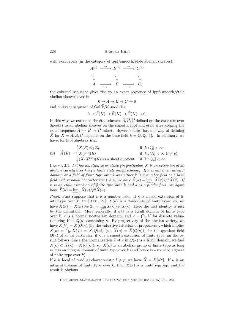
with exact rows (in the category of fppf/smooth/etale abelian sheaves):

A(p) →−−−−→ B(p) ։

−−−−→ C(p)

∩

y ∩

y ∩

y

A −−−−→→

B −−−−→։

C,

the cokernel sequence gives rise to an exact sequence of fppf/smooth/etaleabelian sheaves over k:

0→ A→ B → C → 0

and an exact sequence of Gal(k/k)-modules

0→ A(K)→ B(K)→ C(K)→ 0.

In this way, we extended the etale sheaves A, B, C defined on the etale site overSpec(k) to an abelian sheaves on the smooth, fppf and etale sites keeping the

exact sequence A → B ։ C intact. However note that our way of defining

X for X = A,B,C depends on the base field k = Q,Qp,Ql. In summary, wehave, for fppf algebras R/k:

(S) X(R) =

X(R)⊗Z Zp if [k : Q] <∞,

X [p∞](R) if [k : Ql] <∞ (l 6= p),

(X/X(p))(R) as a sheaf quotient if [k : Qp] <∞.

Lemma 2.1. Let the notation be as above (in particular, X is an extension of anabelian variety over k by a finite etale group scheme). If κ is either an integraldomain or a field of finite type over k and either k is a number field or a local

field with residual characteristic l 6= p, we have X(κ) = lim←−n

X(κ)/pnX(κ). If

κ is an etale extension of finite type over k and k is a p-adic field, we again

have X(κ) = lim←−n

X(κ)/pnX(κ).

Proof. First suppose that k is a number field. If κ is a field extension of fi-nite type over k, by [RTP, IV], X(κ) is a Z-module of finite type; so, we

have X(κ) = X(κ) ⊗Z Zp = lim←−

X(κ)/pnX(κ). Here the first identity is just

by the definition. More generally, if κ/k is a Krull domain of finite typeover k, κ is a normal noetherian domain; and κ =

⋂V V for discrete valua-

tion ring V in Q(κ) containing κ. By projectivity of the abelian variety, wehave X(V ) = X(Q(κ) (by the valuative criterion of properness), which implies

X(κ) =⋂

V X(V ) = X(Q(κ)) (so, X(κ) = X(Q(κ))) for the quotient fieldQ(κ) of κ. In particular, if κ is a smooth extension of finite type, an the re-sult follows, Since the normalization κ of κ in Q(κ) is a Krull domain, we find

X(κ) ⊂ X(κ) = X(Q(κ)); so, X(κ) is an abelian group of finite type as longas κ is an integral domain of finite type over k (and hence is a reduced algberaof finite type over k).

If k is local of residual characteristic l 6= p, we have X = X [p∞]. If κ is an

integral domain of finite type over k, then X(κ) is a finite p-group, and theresult is obvious.



The case where k is local of residual characteristic p is already dealt with beforethe lemma.

For a sheaf X under the topology ?, we write H•? (X) for the cohomology group

H1? (Spec(κ), X) under the topology ?. If we have no subscript, H1(X) means

the Galois cohomology H•(Gal(K/κ), X) for the Gal(K/κ)-module X .

Lemma 2.2. Let X be an extension of an abelian variety over k by a finite etalegroup scheme of order prime to p. For any intermediate extension K/κ/k, Wehave a canonical injection

lim←−n

X(κ)/pnX(κ) → lim←−n

H1(X [pn]).

Similarly, for any fppf, smooth or etale extension κ/k of finite type which is anintegral domain, we have an injection

lim←−n

X(κ)/pnX(κ) → lim←−n

H1? (X [pn])

for ? = fppf, sm or et according as κ/k is an fppf extension or a smoothextension.

By Lemma 2.1, we have X(κ) = lim←−n

X(κ)/pnX(κ) in the following cases:

(2.2)

[k : Q] <∞ and κ is an integral domain of finite type over k

[k : Ql] <∞ with l 6= p and κ is an integral domain of finite type over k

[k : Qp] <∞ and κ is a finite algebraic extension over k.

Proof. We consider the sheaf exact sequence under the topology ? = fppf orsm or etale on Spec(κ)

0→ X [pn]→ Xpn

−→ X.

We want to show that the multiplication by pn is surjective. If our cohomologytheory is Galois cohomology (or equivalently ? = etale), we have an exactsequence

0→ X [pn](K)→ X(K)pn

−→ X(K)→ 0.

Since X(K) = X(K)⊗Z Zp, the desired exactness follows.Let κ be an fppf extension of k. Then for each x ∈ X(κ), we consider theCartesian diagram

Xx −−−−→ Xy

ypn

Spec(κ) −−−−→x

X.

Then Xx∼= X [pn] as schemes over κ; so, Xx = Spec(R) for an etale finite

extension R of κ, which is obviously smooth and also fppf extension of κ. Thusover the coveringR/κ, x is the image of the point given by Spec(R) → X . Then

by [ECH, II.2.5 (c)], Xpn

−→ X is an epimorphism of sheaves under etale, smooth


230 Haruzo Hida

and also fppf topology. If k is a number field, we have X(κ) = X(κ)⊗Z Zp, we

get the exactness of X [pn] → X ։ X from the exactness of X [pn] → X ։ X .If k is a finite extension of Ql for l 6= p, we can argue as above replacing X

by X = X [p∞] and get the exactness of X [pn] → X ։ X. Suppose that k

is a finite extension of Qp. Then X = X/X(p) as a ?-sheaf. Take x ∈ X(κ).Then by definition, we have an ?-extension R of κ such that x is the image ofy ∈ X(R). Then as above we can find a ?-extension R′/R such that y = pny′ for

y′ ∈ X(R′). Then for the image x′ of y′ ∈ X(R′) in X(R′), we have pnx′ = x.

Thus again Xpn

−→ X is an epimorphism of sheaves under the topology ?.Thus we can apply Kummer theory to the sheaf exact sequence

0→ X [pn] → Xpn

−→ X → 0

with respect to the topology given by ?, we have an inclusion

X(κ)/pnX(κ) → H1? (X [pn]). Passing to the limit with respect to n, we

have δ : lim←−n

X(κ)/pnX(κ)→ lim←−n

H1? (X [pn]). Since taking projective limit is

a left exact functor, δ is injective as desired.

Taking instead an injective limit, we get

Lemma 2.3. Let A be an abelian variety over k. For any intermediate extensionK/κ/k, we have an exact sequence

0→ A(κ)⊗Zp Tp → H1? (A[p

∞])→ H1? (A)→ 0

for ? = fppf, sm or et according as κ/k is an fppf extension, a smooth extension

or an etale extension. In particular, the Pontryagin dual of H1? (A) is a Zp-

module of finite type; so, H1? (A) has the form (Qp/Zp)

j⊕∆ for some 0 ≤ j ∈ Zand a finite p-group ∆.

Proof. Since any smooth covering has finer etale covering, we have H•sm(A) =

H•et(A) (cf. [ECH, III.3.4 (c)]). Since an etale covering is covered by a finer etale

finite coverings, Hqet(A) and Hq(A) for q > 0 is a torsion module. This torsion-

ness is well known for Galois cohomology (as the Galois group is profinite; see[CNF, (1.6.1)]).

Pick any x ∈ A(κ). We can find an etale finite extension κ′/κ such that

pny = x for some y ∈ A(κ′). Then y is unique modulo A[pn](κ′). Therefore,

the sheaf quotient (A/A[p∞])(κ) is p-divisible and torsion-free; so, is a sheaf of

Qp-vector spaces. In other words, A/A[p∞] is isomorphic to the sheaf tensor

product A⊗Zp Qp. Thus we have an exact sequence

0→ A[p∞]→ A→ A⊗Zp Qp → 0.

Since H1? (A ⊗Zp Qp) is a Qp-vector space, the image in H1

? (A ⊗Zp Qp) of the

torsion module H1(A) vanishes. Thus we have an exact sequence

0→ A(κ)⊗Zp Tp → H1? (A[p

∞])→ H1? (A)→ 0.



Since 0 → A(κ) ⊗Zp Z/pZ → H1? (A[p]) → H1

? (A)[p] → 0 is exact, by the

finiteness of H1(A[p]) = H1(A[p]) (see [ADT, I.5]), the last assertion for Galoiscohomology follows. Then using the comparison theorem (cf. [ECH, III.3.4 (c)and III.3.9]), we conclude the same for other topologies.

3. U(p)-isomorphisms

We recall the results in [H14b, §3] with detailed proofs for some results anda brief account for some others (as [H14b] is being written along with this

paper). For Z[U ]-modules X and Y , we call a Z[U ]-linear map Xf−→ Y a

U -injection (resp. a U -surjection) if Ker(f) is killed by a power of U (resp.Coker(f) is killed by a power of U). If f is both U -injection and U -surjection,we call f is a U -isomorphism. Thus, f is a U -injection (resp. a U -surjection, aU -isomorphism) if after tensoring Z[U,U−1], it becomes an injection (resp. asurjection, an isomorphism). In terms of U -isomorphisms, we describe brieflythe facts we study in this article (and in later sections, we fill in more detailsin terms of the ordinary projector e).Let N be a positive integer prime to p. We assume Npr ≥ 4 (without losing anygenerality as remarked in the introduction). We consider the (open) modularcurve Y1(Npr)/Q which classifies elliptic curves E with an embedding φ : µpr →

E[pr] = Ker(pr : E → E). Let Ri = Z(p)[µpi ], Ki = Q[µpi ], R∞ =⋃

iRi ⊂ Q

and K∞ =⋃

iKi ⊂ Q. For a valuation subring or a subfield R of K∞ overZ(p) with quotient field K, we write Xr/R for the normalization of the j-line

P(j)/R in the function field of Y1(Npr)/K . The group z ∈ (Z/prZ)× acts on

Xr by φ 7→ φz, as Aut(µNpr ) ∼= (Z/NprZ)×. Thus Γ = 1+pZp = γZp acts onXr (and its Jacobian) through its image in (Z/NprZ)×. Only in the followingsection, we need the result over a discrete valuation ring R. Hereafter, in mostcases, we take U = U(p) for the Hecke-Atkin operator U(p) (though we takeU = U∗(p) sometimes for the dual U∗(p) of U(p)).Let Jr/R = Pic0Xr/R be the connected component of the Picard scheme. Westate a result comparing Jr/R and the Neron model of Jr/K over R. Thuswe assume that R is a valuation ring. By [AME, 13.5.6, 13.11.4], Xr/R isregular; the reduction Xr ⊗R Fp is a union of irreducible components, and thecomponent containing the∞ cusp has geometric multiplicity 1. Then by [NMD,Theorem 9.5.4], Jr/R gives the identity connected component of the Neronmodel of the Jacobian of Xr/R. We write Xs

r/R for the normalization of the

j-line in the function field of the canonical Q-curve associated to the modularcurve of the congruence subgroup Γr

s = Γ1(Npr) ∩ Γ0(ps) (for 0 < r ≤ s). The

open curve Y rs/Q = Xr

s/Q − cusps classifies triples (E,C, φ : µNpr → E) with

a cyclic subgroup C of order ps containing the image φ(µpr ).


232 Haruzo Hida

We denote Pic0Xrs /R

by Jrs/R. Similarly, as above, Jr

s/R is the connected com-

ponent of the Neron model of Xrs/K . Note that

(3.1) Γrs\Γ

rs

(1 00 ps−r

)Γ1(Npr)

=(

1 a0 ps−r

) ∣∣∣a mod ps−r= Γ1(Npr)\Γ1(Npr)

(1 00 ps−r

)Γ1(Npr).

Write Usr (p

s−r) : Jsr/R → Jr/R for the Hecke operator of Γs

rαs−rΓ1(Npr) for

αm =(1 00 pm

). Strictly speaking, the Hecke operator induces a morphism of the

generic fiber of the Jacobians and then extends to their connected componentsof the Neron models by the functoriality of the model (or equivalently by Picardfunctoriality). Then we have the following commutative diagram from theabove identity, first over C, then over K and by Picard functoriality over R:

(3.2)

Jr/Rπ∗

−→ Jrs/R

↓ u ւ u′ ↓ u′′

Jr/Rπ∗

−→ Jrs/R,

where the middle u′ is given by Usr (p

s−r) and u and u′′ are U(ps−r). Thus

(u1) π∗ : Jr/R → Jrs/R is a U(p)-isomorphism (for the projection π : Xr

s →

Xr).

Taking the dual U∗(p) of U(p) with respect to the Rosati involution associatedto the canonical polarization on the Jacobians. We have a dual version of theabove diagram for s > r > 0:

(3.3)

Jr/Rπ∗←− Jr

s/R

↑ u∗ ր u′∗ ↑ u′′∗

Jr/Rπ∗←− Jr

s/R.

Here the superscript “∗” indicates the Rosati involution corresponding to thecanonical divisor on the Jacobians, and u∗ = U∗(p)s−r for the level Γ1(Npr)and u′′∗ = U∗(p)s−r for Γr

s. Note that these morphisms come from the followingdouble coset identity:

(3.4) Γrs\Γ

rs

(ps−r 00 1

)Γ1(Npr)

=(

ps−r a0 1

) ∣∣∣a mod ps−r= Γ1(Npr)\Γ1(Npr)

(ps−r 00 1

)Γ1(Npr).

From this, we get

(u∗1) π∗ : Jrs/R → Jr/R is a U∗(p)-isomorphism, where π∗ is the dual of π∗.

In particular, if we take the ordinary and the co-ordinary projector e =limn→∞ U(p)n! and e∗ = limn→∞ U∗(p)n! on J [p∞] for J = Jr/R, Js/R, J

rs/R,

noting U(pm) = U(p)m, we have

π∗ : Jordr/R[p

∞] ∼= Jr,ords/R [p∞] and π∗ : Jr,co-ord

s/R [p∞] ∼= Jco-ordr/R [p∞]



where “ord” (resp. “co-ord”) indicates the image of the projector e (resp. e∗).For simplicity, we write Gr/R := Jord

r/R[p∞]/R.

Suppose that we have morphisms of three noetherian schemes Xπ−→ Y

g−→ S

with f = g π. We look into

H0fppf(T,R

1f∗Gm) = R1f∗O×X(T ) = PicX/S(T )

for S-scheme T and the structure morphism f : X → S (see [NMD, Chapter 8]).

Suppose that f and g have compatible sections Ssg−→ Y and S

sf−→ X so that

π sf = sg. Then we get (e.g., [NMD, Section 8.1])

PicX/S(T ) = Ker(s1f : H1fppf(XT , O

×X)→ H1

fppf(T,O×T ))

PicY/S(T ) = Ker(s1g : H1fppf(YT , O

×YT

)→ H1fppf(T,O

×T ))

for any S-scheme T , where sqf : Hqfppf(XT , O

×XT

) → Hqfppf(T,O

×T ) and sng :

Hnfppf(YT , O

×YT

) → Hnfppf(T,O

×T ) are morphisms induced by sf and sg, respec-

tively. Here we wrote XT = X ×S T and YT = Y ×S T . We suppose thatthe functors PicX/S and PicY/S are representable by smooth group schemes(for example, if X,Y are curves and S = Spec(k) for a field k; see [NMD,Theorem 8.2.3 and Proposition 8.4.2]). We then put J? = Pic0?/S (? = X,Y ).

Anyway we suppose hereafter also that X,Y, S are varieties (in the sense of[ALG, II.4]).For an fppf covering U → Y and a presheaf P = PY on the fppf site over Y ,we define via Cech cohomology theory an fppf presheaf U 7→ Hq(U , P ) denoted

by Hq(PY ) (see [ECH, III.2.2 (b)]). The inclusion functor from the category

of fppf sheaves over Y into the category of fppf presheaves over Y is left exact.The derived functor of this inclusion of an fppf sheaf F = FY is denoted byH•(FY ) (see [ECH, III.1.5 (c)]). Thus H•(Gm/Y )(U) = H•

fppf(U , O×U ) for a

Y -scheme U as a presheaf (here U varies in the small fppf site over Y ).Assuming that f , g and π are all faithfully flat of finite presentation, we usethe spectral sequence of Cech cohomology of the flat covering π : X ։ Y inthe fppf site over Y [ECH, III.2.7]:

(3.5) Hp(XT /YT , Hq(Gm/Y ))⇒ Hn

fppf(YT , O×YT

)∼−→ι

Hn(YT , O×YT

)

for each S-scheme T . Here F 7→ Hnfppf(YT , F ) (resp. F 7→ Hn(YT , F )) is

the right derived functor of the global section functor: F 7→ F (YT ) from thecategory of fppf sheaves (resp. Zariski sheaves) over YT to the category ofabelian groups. The canonical isomorphism ι is the one given in [ECH, III.4.9].By the sections s?, we have a splitting Hq(XT , O

×XT

) = Ker(sqf ) ⊕Hq(T,O×T )

and Hn(YT , O×YT

) = Ker(sng ) ⊕ Hn(T,O×T ). Write H•

YTfor H•(Gm/YT

) and

H•(H0YT

) for H•(YT /XT , H0YT

). Since

PicX/S(T ) = Ker(s1f,T : H1(XT , O×XT

)→ H1(T,O×T ))

for the morphism f : X → S with a section [NMD, Proposition 8.1.4], fromthis spectral sequence, we have the following commutative diagram with exact


234 Haruzo Hida

rows, writing H0(XT

YT, ?) as H0(?) and H1(T,O×

T ) as H1(O×

T ):

(3.6)?1 −−−−→ H1(H0

YT) H1(H0

YT)

yy

y∩

PicT ⊕JY (T )→

−−−−→ PicT ⊕PicY/S(T )∼

−−−−→ H1(O×T )⊕Ker(s1g,T )

c

y b

y a

y

PicT ⊕H0(JX(T ))

→−−−−→ H0(PicY (T )) H0(H1(Gm,Y ))y

yy

?2 −−−−→ H2(H0YT

) H2(H0YT

),

where we have written J? = Pic0?/S (the identity connected component of

Pic?/S). Here the vertical exactness at the right two columns follows fromthe spectral sequence (3.5) (see [ECH, Appendix B]).

We now recall the definition of the Cech cohomology: for a general S-scheme

T and Cech cochain ci0,...,iq ∈ H0(X(q+1)T , O×

X(q+1)T

),

(3.7) Hq(XT

YT, H0(Gm/Y )) =

(ci0,...,iq )|∏

j(ci0...ij ...iq+1 pi0...ij ...iq+1

)(−1)j = 1

dbi0...iq =∏

j(bi0...ij ...iq pi0...ij ...iq )(−1)j |bi0...ij ...iq ∈ H0(X

(q)T , O×

X(q)T

)

where we agree to put H0(X(0)T , O

(0)XT

) = 0 as a convention,

X(q)T =

q︷︸︸︷X ×Y X ×Y · · · ×Y X ×ST,

OX

(q)T

=

q︷︸︸︷OX ×OY OX ×OY · · · ×OY OX ×OSOT ,

the identity∏

j(cpi0...ij ...iq+1)(−1)j = 1 takes place in O

X(q+2)T

and pi0...ij ...iq+1:

X(q+2)T → X

(q+1)T is the projection to the product of X the j-th factor removed.

Since T×T T ∼= T canonically, we haveX(q)T∼=

q︷︸︸︷XT ×T · · · ×T XT by transitivity

of fiber product.Take a correspondence U ⊂ Y ×S Y given by two finite flat projections π1, π2 :U → Y of constant degree (i.e., πj,∗OU is locally free of finite rank deg(πj) over



OY ). Consider the pullback UX ⊂ X ×S X given by the Cartesian diagram:

UX = U ×Y×SY (X ×S X) −−−−→ X ×S Xy

y

U→

−−−−→ Y ×S Y

Let πj,X = πj ×S π : UX ։ X (j = 1, 2) be the projections.We describe the correspondence action of U on H0(X,O×

X) in down-to-earthterms. Consider α ∈ H0(X,OX). Then we lift π∗

1,Xα = α π1,X ∈

H0(UX ,OUX ). Put αU := π∗1,Xα. Note that π2,X,∗OUX is locally free of rank

d = deg(π2) overOX , the multiplication by αU has its characteristic polynomialP (T ) of degree d with coefficients in OX . We define the norm NU (αU ) to bethe constant term P (0). Since α is a global section, NU (αU ) is a global section,as it is defined everywhere locally. If α ∈ H0(X,O×

X), NU (αU ) ∈ H0(X,O×X).

Then define U(α) = NU (αU ), and in this way, U acts on H0(X,O×X).

For a degree q Cech cohomology class [c] ∈ Hq(X/Y , H0(Gm/Y )) of a Cech

q-cocycle c = (ci0,...,iq ), U([c]) is given by the cohomology class of the Cech co-cycle U(c) = (U(ci0,...,iq )), where U(ci0,...,iq ) is the image of the global sectionci0,...,iq under U . Indeed, (π∗

1,Xci0,...,iq ) plainly satisfies the cocycle condition,

and (NU (π∗1,Xci0,...,iq )) is again a Cech cocycle as NU is a multiplicative homo-

morphism. By the same token, we see that this operation sends coboundariesto coboundaries and obtain the action of U on the cohomology group.

Lemma 3.1. Let the notation and the assumption be as above. In particular,π : X → Y is a finite flat morphism of geometrically reduced proper schemesover S = Spec(k) for a field k. Suppose that X and UX are proper schemesover a field k satisfying one of the following conditions:

(1) UX is geometrically reduced, and for each geometrically connected com-ponent X of X, its pull back to UX by π2,X is also connected; i.e.,

π0(X)π∗

2,X−−−→

∼π0(UX);

(2) (f π2,X)∗OUX = f∗OX .

If π2 : U → Y has constant degree deg(π2), the action of U on H0(X,O×X)

factors through the multiplication by deg(π2) = deg(π2,X).

Proof. By properness, under (1) or (2), H0(UX ,OUX )π2,X,∗= H0(X,OX)(

(1)=

kπ0(X)) for the set of connected components π0(X) of X . In particular, we see

αU ∈ H0(UX ,OUX ) = H0(X,OX), which tells us that NU (αU ) = αdeg(π2)U , and

the result follows.

Consider the iterated product πi,X(q) = πi,X ×Y · · · ×Y πi,X : U(q)X → X(q)

(i = 1, 2). Here U(q)X =

q︷︸︸︷UX ×Y UX ×Y · · · ×Y UX . We plug in U

(j)X in the first


236 Haruzo Hida

j slots of the fiber product (for 0 < j ≤ q) and consider

U(j−1)X ×Y X(q−j+1)

π(q)1,j←−− Uj := U

(j)X ×Y X(q−j)

π(q)2,j−−→ U

(j−1)X ×Y X(q−j+1)

which induces a correspondence Uj in (U(j−1)X ×Y X(q−j+1)) ×Y (U

(j−1)X ×Y

X(q−j+1)). Here πi,j restricted to first j − 1-factors UX is the identity idUX ;the last q−j factors is the identity idX and at the j-th factor, it is the projectionπi (i = 1, 2). For example, if q = 3 and i = 2, we have

UX ×Y UX ×Y UX

π(q)2,3

−−−−−−−−−→idU × idU ×π2

UX ×Y UX ×Y X

π(q)2,2

−−−−−−−−→idU ×π2×idX

UX ×Y X ×Y Xπ(q)2,1

−−−−−−−−−→π2×idX × idX

X ×Y ×Y X.

Naturally π2,X(q) factors through the following q consecutive coverings Uqρq−→

Uq−1ρq−1−−−→ · · ·

ρ1−→ X(q) for ρj = π

(q)2,j . Note that the norm map NUq =

Nπ2,X(q)

: π2,X(q),∗O×Uq→ O×

X(q) factors through the corresponding norm maps:

NUq = Nq Nq−1 · · · N1,

where Nj is the norm map with respect to Uj → Uj−1. The last norm is

essentially the product of NU and the identity of X(q−1) corresponding toU ×Y X(q−1)

։ X(q). In particular, ρ1,∗(OU1 ) = π2,X,∗(OUX ) ⊗OY OX(q−1)

and

(f ρ1)∗(OU1 ) = (f π2,X)∗(OUX )⊗OY

q−1︷︸︸︷f∗OX ⊗OY · · · ⊗OY f∗OX .

Thus if the assumption (2) in Lemma 3.1 is satisfied, the corresponding assump-tion for U1 is satisfied. The assumption (1) implies (2) which is really necessaryfor the proof of Lemma 3.1. Applying the argument proving Lemma 3.1 to thecorrespondence U1 and the last factor N1 of the norm, we get

Corollary 3.2. Let the notation and the assumption be as in Lemma 3.1.Then the action of U (q) on H0(X,O×

X(q)) factors through the multiplication bydeg(π2) = deg(π2,X).

Here is a main result of this section:

Proposition 3.3. Suppose that S = Spec(k) for a field k. Let π : X → Ybe a finite flat covering of (constant) degree d of geometrically reduced proper

varieties over k, and let Yπ1←− U

π2−→ Y be two finite flat coverings (of constant

degree) identifying the correspondence U with a closed subscheme Uπ1×π2→ Y ×S

Y . Write πj,X : UX = U ×Y X → X be the base-change to X. Suppose one ofthe conditions (1) and (2) of Lemma 3.1 for (X,U). Then

(1) The correspondence U ⊂ Y ×SY sends Hq(H0Y ) into deg(π2)(H

q(H0Y ))

for all q > 0.(2) If d is a p-power and deg(π2) is divisible by p, Hq(H0

Y ) for q > 0 iskilled by UM if pM ≥ d.



(3) The cohomology Hq(H0Y ) with q > 0 is killed by d.

Proof. The first assertion follows from Corollary 3.2. Indeed, by (3.7), U (q) actson each Cech q-cocycle, through an action factoring through the multiplicationby deg(π2,X) = deg(π2) by Corollary 3.2.

Now we regard Xπ−→ Y as a correspondence of Y (with multiplicity d)

by the projection π1 = π2 = π : X → Y . Then [X ](c) = dc forc ∈ Hq(X/Y,H0(Gm/Y )). On the other hand, by the definition of the cor-

respondence action, [X ] factors through Hq(X/X,H0(Gm/Y )) = 0, and hence

dx = 0. This shows that if X/Y is a covering of degree d, Hq(X/Y,H0(Gm/Y ))is killed by d proving (3), and the assertion (2) follows from the first (1).

We apply the above proposition to (U,X, Y ) = (U(p), Xs, Xrs ) with U given

by U(p) ⊂ Xrs × Xr

s over Q. Indeed, U := U(p) ⊂ Xrs × Xr

s correspondsto X(Γ) given by Γ = Γ1(Npr) ∩ Γ0(p

s+1) and UX is given by X(Γ′) forΓ′ = Γ1(Nps) ∩ Γ0(p

s+1) both geometrically irreducible curves. In this caseπ1 is induced by z 7→ z

p on the upper complex plane and π2 is the natural

projection of degree p. In this case, deg(Xs/Xrs ) = ps−r and deg(π2) = p.

Assume that a finite group G acts on X/Y faithfully. Then we have a naturalmorphism φ : X ×G→ X ×Y X given by φ(x, σ) = (x, σ(x)). In other words,we have a commutative diagram

X ×G(x,σ) 7→σ(x)−−−−−−−→ X

(x,σ) 7→x

yy

X −−−−→ Y,

which induces φ : X ×G → X ×Y X by the universality of the fiber product.Suppose that φ is surjective; for example, if Y is a geometric quotient of Xby G; see [GME, §1.8.3]). Under this map, for any fppf abelian sheaf F , wehave a natural map H0(X/Y, F ) → H0(G,F (X)) sending a Cech 0-cocyclec ∈ H0(X,F ) = F (X) (with p∗1c = p∗2c) to c ∈ H0(G,F (X)). Obviously, bythe surjectivity of φ, the map H0(X/Y, F )→ H0(G,F (X)) is an isomorphism(e.g., [ECH, Example III.2.6, page 100]). Thus we get

Lemma 3.4. Let the notation be as above, and suppose that φ is surjective. Forany scheme T fppf over S, we have a canonical isomorphism: H0(XT /YT , F ) ∼=H0(G,F (XT )).

We now assume S = Spec(k) for a field k and that X and Y are proper reducedconnected curves. Then we have from the diagram (3.6) with the exact middle


238 Haruzo Hida

two columns and exact horizontal rows:

0 −−−−→ Z Z −−−−→ 0x deg

xonto deg

xonto

x

H1(H0Y ) −−−−→ PicY/S(T )

b−−−−→ H0(XT

YT,PicY/S(T )) −−−−→ H2(H0

Y )x ∪

xx∪

x

?1 −−−−→ JY (T ) −−−−→c

H0(XT

YT, JX(T )) −−−−→ ?2,

Thus we have ?j = Hj(H0Y ) (j = 1, 2).

By Proposition 3.3, if q > 0 and X/Y is of degree p-power and p| deg(π2),Hq(H0

Y ) is a p-group, killed by UM for M ≫ 0. Taking (X,Y, U)/S to be(Xs/Q, X

rs/Q, U(p))/Q for s > r ≥ 1 for p odd and s > r ≥ 2 for p = 2, we get

for the projection π : Xs → Xrs

Corollary 3.5. Let F be a number field or a finite extension of Ql (for aprime l not necessarily equal to p). Then we have

(u) π∗ : Jrs/Q(F )→ H0(Xs/X

rs , Js/Q(F ))

(∗)= Js/Q(F )[γpr−1

− 1] is a U(p)-

isomorphism,

where Js/Q(F )[γpr−1

− 1] = Ker(γpr−1

− 1 : Js(F )→ Js(F )).

From these, we got the following facts as [H14b, Lemma 3.7]

Lemma 3.6. We have morphisms

ιrs : Js/Q[γpr−1

− 1]→ Jrs/Q and ιr,∗s : Jr

s/Q → Js/Q/(γpr−1

− 1)(Js/Q)

satisfying the following commutative diagrams:

(3.8)

Jrs/Q

π∗

−→ Js/Q[γpr−1

− 1]

↓ u ւ ιrs ↓ u′′

Jrs/Q

π∗

−→ Js/Q[γpr−1

− 1],

and

(3.9)

Jrs/Q

π∗←− Js/Q/(γpr−1

− 1)(Js/Q)

↑ u∗ ր ιr,∗s ↑ u′′∗

Jrs/Q

π∗

←− Js/Q/(γpr−1

− 1)(Js/Q),

where u and u′′ are U(ps−r) = U(p)s−r and u∗ and u′′∗ are U∗(ps−r) =U∗(p)s−r. In particular, for an fppf extension T/Q, the evaluated map at T :

(Js/Q/(γpr−1

− 1)(Js/Q))(T )π∗−→ Jr

s (T ) (resp. Jrs (T )

π∗

−→ Js[γpr−1

− 1](T )) is aU∗(p)-isomorphism (resp. U(p)-isomorphism).

Remark 3.7. Note here that the natural morphism:

Js(T )

(γpr−1 − 1)(Js(T ))→ (Js/(γ

pr−1

− 1)(Js))(T )



may have non-trivial kernel and cokernel which may not be killed by a powerof U∗(p). In other words, the left-hand-side is an fppf presheaf (of T ) and the

right-hand-side is its sheafication. On the other hand, T 7→ Js[γpr−1

− 1](T )

is already an fppf abelian sheaf; so, Jr(T )π∗

−→ Js[γpr−1

− 1](T ) is a U(p)-isomorphism without ambiguity by the above Lemma 3.6 and Corollary 3.5

combined. Also, as remarked in the introduction, we need to replace γpr−1

− 1

in the above statement by γpr−2

− 1 if p = 2.

4. Structure of Λ-BT groups over number fields and local fields

Let G/R∞:= lim−→r

Jr[p∞]ord/R∞

, which is a Λ-BT group in the sense of [H14a,

Sections 3 and 5] with a canonical h-action. Here for an abelian variety A/R,

A[pn] = Ker(Apn

−→ A) and A[p∞]/R = lim−→n

A[pn] (the p-divisible Barsotti–

Tate group of A over R). For an h-algebra A, we put GA = G ⊗h A. Pick areduced local ring T of h and write a(lm) for the image in T of U(lm) or T (lm)for a prime l according as l|Np or l ∤ Np and mT for the maximal ideal of T.Since GT is a Λ-BT group in the sense of [H14a, Theorem 5.4, Remark 5.5], wehave the connected-etale exact sequence over Zp[µp∞ ]:

0→ GT → GT → GetT → 0,

where GT is the connected component of the flat group GT and G etT is the quotientof GT by GT. The etale group GT/Q over Q is a Λ-BT group over Q (in the sense

of [H14a, §4]) on which Z×p act by diamond operators. The entire group GT

extends to a Λ-BT group over Zp[µp∞ ] (see [H14a, Remark 5.5]). The Qp-pointsof this sequence descent to Qp giving an exact sequence:

0→ GT(Qp)→ GT(Qp)→ GetT (Qp)→ 0

with G etT (Qp) = H0(Ip,GT(Qp)) for the inertia group Ip ⊂ Gal(Qp/Qp).

We know that GT and G etT are well controlled, and the Pontryagin dual modules

of GT(Q) and G etT (Q) are Λ-free modules of (equal) finite rank (see [H86b, §9]or [H14a, Sections 4–5]). Here we equip these Λ-divisible modules with thediscrete topology. Take a field k as a base field. Pick a T-ideal a. Write GT[a]for the kernel of a:

GT[a](R) = x ∈ GT(R)|ax = 0 ∀a ∈ a,

where R is an fppf extension of k. Write a(p) for the image of U(p) in T.For the moment, assume that k is a finite extension k of Qp with p-adic integerring W . If the residual degree of k is f and a(p)f 6≡ 1 mod mT for the maximalideal mT of T, we have

GT[mT]et(k) = 0,

since the action of Frobp on GT[mT]et(Qp) is given by multiplication by a(p). On

the other hand, the action of Gal(k/k) on e · J∞[p∞](k)⊗h T factors throughGal(k[µp∞ ]/k) → Z×

p → Λ×, where the factor Γ = 1+pZp of Z×p = Γ×µp−1 is


240 Haruzo Hida

embedded into Λ = Zp[[Γ]] by natural inclusion and ζ ∈ µp−1 is sent to ζa forsome 0 ≤ a =: a(T) = ak(T) < p−1. Thus if a(T) 6= 0, we have GT[mT](k) = 0.We have a natural projection π = πr

s : Gs := Js[p∞]ord/Q → Gr for s > r (see

[H13a, Section 4] where πrs is written as Ns

r ). This induces a projective systemof Tate modules TGs,T := TGs ⊗h Ts and TG?s,T for ? = , et. We put

TG?T = lim←−s

TG?s,T(Q) for ? = nothing, or et. They are Λ-free modules with a

continuous action of Gal(Q/Q). Write ρT for the Galois representation realizedon TGT, and put ρP = ρT mod P acting on TGT/PTGT for P ∈ Spec(T). Inparticular, we simply write ρ = ρT = ρmT

for the maximal ideal mT of T.If T is a Gorenstein ring, then for the Tate modules TGT, TG

T and TG etT as

above, we have

TGT ∼= T2 and TGT∼= T ∼= TG etT

as T-modules (e.g., [H13a, Section 4]), and if ρT(Ip) contains a non-trivial

unipotent element for the inertia group Ip in Gal(Qp/k), again we have

G etT [mT](k) = 0. Thus we get

Lemma 4.1. Let k/Qpin Qp be a finite extension and T be a reduced local

ring of h. Assume that k has residual degree f and one of the following twoconditions:

(1) ak(T) 6= 0 and a(p)f 6≡ 1 mod mT,(2) T is a Gorenstein ring, and ρT(Ip) has non-trivial unipotent element

for the inertia group Ip of Gal(Qp/k).

Then we have GT(k) = 0.

Proof. Let V be the Λ-dual of TGT, which is also the Pontryagin dual of GT.Then we haveH0(k, V/mTV ) ∼= GT[mT](k) = H0(k,GT[mT]). By the assumption(1) or (2), we have the vanishing GT[mT](k) = 0. Look into the following exactsequence of sheaves

0→ GT[mT]→ GTϕ−→

⊕

α∈I

GT

with ϕ(x) = (αx)α for a finite set I = αα of generators of mT. Taking theGal(k/k)-invariant, we get another exact sequence

0→ GT[mT](k)→ GT(k)ϕk−−→

⊕

α∈I

GT(k).

Since Ker(ϕk) = GT(k)[mT], we conclude (GT(k))[mT] = GT[mT](k) = 0. Takingthe Pontryagin dual module written as M∨ for a compact or discrete moduleM , we have, setting V = GT(Q)∨,

H0(k, V )/mTH0(k, V ) ∼= (GT(k))∨/mT(GT(k))

∨ = (GT(k)[mT])∨ = 0,

which implies GT(k)∨ = H0(k, V ) = 0 by Nakayama’s lemma, and hence

GT(k) = 0. This proves the assertion under (1) or (2).

In the l 6= p case, we remark the following fact:



Lemma 4.2. Let k/Qlin Ql be a finite extension for a prime l 6= p and T be a

reduced local ring of h. If the semi-simplification of GT[mT] as a representationof Gal(Ql/k) does not contain the identity representation, then GT(k) = 0. Ingeneral, GT(k)

∨ is always a torsion Λ-module of finite type.

Proof. If the semi-simplification of GT[mT] as a representation of Gal(Ql/k)does not contain the identity representation, we have H0(k,GT[mT]) = 0; so,H0(k, V/mTV ) = 0 for V = GT(Q)∨. Writing mT = (αi)i∈I for αi ∈ T with afinite index set I, we have an exact sequence:

0→ GT[mT](Q)→ GT(Q)x 7→(αix)i−−−−−−→

⊕

i∈I

GT(Q).

Taking the Pontryagin dual we have another exact sequence of Galois modules:

0← V/mTV ← Vx 7→(αix)i←−−−−−−

∏

i∈I

V.

Since Galois homology functor is right exact, the above exact sequence implies

H0(k, V )⊗T T/mT = H0(k, V/mTV ) = 0.

Then by Nakayama’s lemma, we get H0(k, V ) = 0, which implies GT(k) = 0.Let f be the residual degree of k as before. Consider the Hecke polynomialHf,l(X) = X2 − A(lf )X + lf 〈l〉f , where A(lf ) is determined by the followingrecurrence relation: A(l) = a(l) and A(lm) = a(lm) − l〈l〉a(lm−1) for m ≥2. If l ∤ Np, GT is unramified over k. By the Eichler–Shimura congruencerelation (e.g. [GME, Theorem 4.2.1]), if l ∤ Np, for the l-Frobenius elementφ ∈ Gal(k/k), the linear operator Hf,l(φ) annihilates GT. Thus if Hf,l(X)

mod mT is not divisible by X−1, GT[mT] as a representation of Gal(Ql/k) doesnot contain the identity representation.For an arithmetic prime P , Hf,l(X) mod P does not have a factor X − 1.Thus after the localization at P of the Pontryagin dual (GT(k)

∨)P is killed byHf,l(φ) and φ− 1, and hence GT(k)

∨ is a torsion Λ-module.Now assume that l|N . By the solution of the local Langlands conjecture (see[C86] and [AAG]), after replacing k by its finite extension, the Galois moduleGT[P ] for an arithmetic point P becomes unramified unless ρP is Steinberg atl (i.e., is multiplicative type at l). Suppose that we have a non-Steinberg P .Then characteristic polynomial H(X) of φ modulo P is prime to X − 1 (asH(X) mod P has Weil numbers of weight f as its roots). Then by the sameargument, we conclude the torsion property.Suppose that all arithmetic point of Spec(T) is Steinberg at l (this often hap-pens; see a remark below Conjecture 3.4 of [H11, §3]). Write ρP for the 2-dimensional Galois representation realized on (GT(Ql)

∨) ⊗T κ(P ). Again byLanglands-Carayol, ρP (Il) for the inertia group Il ⊂ Gal(Ql/k) contains anon-trivial unipotent element. Thus ρP does not have a quotient on which Ilacts trivially. This shows again the Λ-torsion property.


242 Haruzo Hida

Let Spec(I) ⊂ Spec(T) be an irreducible component. Without assuming theGorenstein condition, we have (TGI)P ∼= I2P for almost all height one primesP ∈ Spec(Λ); so, we have ρI with values in GL2(IP ) for most of P . We call I a

CM component if ρI ∼= IndQM Ψ for a Galois character Ψ : Gal(Q/M)→ I×P (foran imaginary quadratic field M). If I is not a CM component, again for almostall P , by [Z14], ρT(Ip) contains an unipotent element conjugate to ( 1 u

0 1 ) with

non-zero-divisor u ∈ T×P . In this case, we have H0(Gal(k/k), TGI)P = 0; so,

GI(k) is a co-torsion Λ-module.

Lemma 4.3. Let k/Qpin Qp be a finite extension with residual degree f and T

be a reduced local ring of h. Then the Pontryagin dual GT(k)∨ of GT(k) is a

torsion Λ–module of finite type.

Proof. We may suppose either a(p)f ≡ 1 mod mT or ak(T) = 0, as otherwiseGT(k) = 0 by Lemma 4.1. Replacing T by its irreducible component I, we onlyneed to prove torsion-ness for GI(k)

∨. Write V for the Λ-torsion free quotientof TGI. Then for any P ∈ Spec(Λ)(Qp), we have VP = (TGI)P (as the reflexiveclosure in [BCM, Chapter 7] of I is Λ-free).If I is not a CM component (i.e., ρI is not an induced representation from theGalois group over an imaginary quadratic field), the assertion follows from thesame argument proving Lemma 4.1 replacing mT by PTP and T by TP . Indeed,taking an arithmetic point P of weight 2. Then by [Z14], we have u ∈ T×

P . ThenH0(k, VP /PVP ) is a submodule of H0(I, VP /PVP ) (for the inertia group I atp) killed by a(p)f − 1. Since P is an arithmetic point of weight 1, we maychoose P so that a(p) mod P is a Weil number of weight 1 (indeed, we onlyneed to assume that the Neben character of fP is non-trivial at p; see [MFM,Theorem 4.6.17]), and hence a(p)f 6≡ 1 mod P . Thus H0(k, VP /PVP ) = 0.This implies GI(k)[P ] is a finite module; so, GI(k)

∨ is a torsion Λ-module.

Now assume that I is a CM component with ρI = IndQM Ψ. Define Ψc(σ) =Ψ(cσc−1) for a complex conjugation c. In the imaginary quadratic field M , psplits into a product of two primes pp as ρI is ordinary. For any arithmeticpoint P ∈ Spec(I)(Qp) ΨP := Ψ mod P ramifies at p and its restriction tothe inertia group at p has infinite order, and Ψc is unramified at p with infiniteorder Ψc(Frobp) (from an explicit description of Ψ; cf, [H13a, §3]). Then wehave VP = V ⊗I IP ∼= I2P. Thus replacing k by the composite kMp, we have

VP∼= Ψ⊕Ψc over Gal(Qp/k). Since Ψc is unramified at p and Ψc

P(Frobp) has

infinite order. This shows that H0(k, VP/PVP) = 0, and again we find thatG∨I (k) is a torsion I-module and hence a torsion Λ-module.

Corollary 4.4. If k is a number field or a finite extension of Ql, the local-ization of GT(k)

∨ at an arithmetic prime of weight 2 vanishes.

Proof. We only need to prove this for a finite extension k of Ql. Write Wfor the integer ring of k. Replacing k by its finite extension, we may assumethat AP has semi-stable reduction over W for an arithmetic prime at P . IfAP has good reduction and l 6= p, the l-Frobenius acts on TpAP by a Weil



number of weight ≥ 1, and then AP [p∞](k) is finite; so, GT[P ](k) is finite. If

l = p, by [Z14], the inertia image in Aut(TpAP ) contains a non-trivial unipotentelement, and hence again AP [p

∞](k) is finite, and the result follows. If AP hasmultiplicative reduction, AP [p

∞](k) is finite by a theorem of Tate–Mumford asthe Tate period of AP is non-trivial. This shows that GT[P ](k) is finite, andhence the result follows.

5. Abelian factors of modular Jacobians

Let hr(Z) be the subalgebra generated by T (n) (including U(l) for l|Np) ofEnd(Jr/Q). Then hr(Zp) = hr(Z) ⊗Z Zp is canonically isomorphic to the Zp-subalgebra of End(Jr[p

∞]) generated by T (n) (including U(l) for l|Np). Thenhr = hr(Zp)

ord by the control theorems in [H86a] and [H86b].

As before, let k be a finite extension of Q inside Q or a finite extension ofQl inside Ql. Let Ar be a abelian subvariety of Jr defined over k. Write As

(s > r) for the image of Ar in Js under the morphism π∗ : Jr → Js givenby Picard functoriality from the projection π : Xs → Xr. If Ar is Shimura’sabelian subvariety attached to a Hecke eigenform f , we sometimes write Af,s

for As to indicate this fact. Hereafter we assume

(A) We have a coherent sequence αs ∈ End(Js/Q) (for all s ≥ r) having thelimit α = lim

←−sαs ∈ End(J∞/Q) such that

(a) As is the connected component of Js[αs] with Js = As+αs(Js) sothat the inclusion: As[p

∞] ∼= Js[αs][p∞] is a U(p)-isomorphism,

(b) the restriction αs|αs(Js) ∈ End(αs(Js)) is a self-isogeny.

Here for s′ > s, coherency of αs means the following commutative diagram:

Jsπ∗

−−−−→ Js′

αs

yyαs′

Js −−−−→π∗

Js′

.

The Rosati involution h 7→ h∗ and T (n) 7→ T ∗(n) (with respect to the canonicaldivisor on Jr) brings hr(Z) to h∗

r(Z) ⊂ End(Jr/Q). Define A∗s to be the identity

connected component of Js[α∗]. The condition (A) is equivalent to

(B) The abelian quotient map Js ։ Bs = Coker(αs) dual to A∗s ⊂ Js

induces an U(p)-isomorphism of Tate modules: Tp(Js/αs(Js))→ TpBs

and αs induces an automorphism of the Qp-vector space Tpαs(Js)⊗Zp

Qp.

Again if Ar is Shimura’s abelian subvariety of Jr associated to a Hecke eigen-form f , we sometimes write Bf,s for Bs as above. The condition (A) (andhence (B)) is a mild condition. Here are sufficient conditions for (α,As, Bs) tosatisfy (A) (and (B)):

Proposition 5.1. Let Spec(T) be a connected component of Spec(h) andSpec(I) be an irreducible component of Spec(T). Then the condition (A) holdsfor the following choices of (α,As, Bs):


244 Haruzo Hida

(P1) Fix r > 0. Then αs = α for a factor α|γpr−1

− 1 in Λ, As = Js[α]

(the identity connected component) and Bs = Pic0As/Q for all s ≥ r.

(P2) Suppose that an eigen cusp form f = fP new at each prime l|N belongsto Spec(T) and that T = I is regular (or more generally a unique fac-torization domain). Then writing the level of fP as Npr, the algebrahomomorphism λ : T → Qp given by f |T (l) = λ(T (l))f gives rise tothe prime ideal P = Ker(λ). Since P is of height 1, it is principalgenerated by ∈ T. This has its image s ∈ Ts = T ⊗Λ Λs for

Λs = Λ/(γps−1

−1). Since hs = h⊗ΛΛs = Ts⊕Xs as an algebra directsum, End(Js/Q) ⊗Z Zp ⊃ hs(Zp) = Ts ⊕ Ys with Ys projecting downonto Xs. Then, we can approximate as = s ⊕ 1s ∈ hs(Zp) for theidentity 1s of Ys by αs ∈ hs(Z) so that αshs(Zp) = ashs(Zp) (hereafterwe call αs “sufficiently close” to as if αshs(Zp) = ashs(Zp)). For thischoice of αs, As := Af,s and Bs := Bf,s.

(P3) More generally than (P2), we pick a general connected componentSpec(T) of Spec(h). Pick a (classical) Hecke eigenform f = fP (ofweight 2) for P ∈ Spec(T). Assume that hs (for every s ≥ r) is re-duced and P = () for ∈ T, and write s for the image of inhs(Zp). Take the complementary direct summand Ys of Ts in hs(Zp)and approximate as := s⊕ 1s in hs(Zp) to get αs sufficiently close toas. Then for this choice of αs, As := Af,s and Bs := Bf,s.

(P4) Suppose that T/() for a non-zero divisor ∈ T is a reduced algebra

of characteristic 0 factoring through hr := h/(γpr−1

− 1)h for somer > 0. Assume that Ts is reduced for every s ≥ r, and write s for theimage of in Ts. Then approximating as = s ⊕ 1s by αs ∈ hs(Z)sufficiently closely for each s ≥ r, we define As to be the connectedcomponent of Js[αs] and Bs to be its dual quotient.

Proof. We first prove (P4). Since αs is sufficiently close to as, we have theidentity αshs(Zp) = ashs(Zp) of ideals. By reducedness of Ts, we have analgebra product decomposition: hs(Qp) := hs(Zp)⊗ZpQp = αs(Ts)⊗ZpQp×Zs

for the complementary Qp-subalgebra Zs, which is given by (Ts/(s))⊗Zp Qp.Write the idempotent of Zs as ǫs ∈ Zs. Then ǫs + as is invertible in hs(Qp).For some positive integer Ms, βs := U(p)Msǫs ∈ hs(Z) ⊂ End(Js). Then byǫs + as ∈ hs(Qp)

×, the connected component As of Js[αs] is given by βs(Js),Js = βs(Js) + αs(Js) = As + α(Js), and the inclusion map As → Js[αs] isan U(p)-isomorphism. Since αs is invertible in αs(hs(Qp)), αs induces a self-isogeny of α(Js). Thus the triple satisfies (A). Since s′hs′(Zp) surjects downto shs(Zp) for all s′ ≥ s, we can adjust αs inductively to have a projectivesystem αs ∈ End(Js)s≥r. Thus α = lim

←−sαs ∈ End(J∞) does the job. This

proves (P4). The assertions (P2) and (P3) are direct consequences of (P4).

As for (P1), since α|(γpr−1

− 1)|(γps−1

− 1) in the unique factorization domainΛ, factoring γps

− 1 = αsβs, the ideals (αs) and (βs) are co-prime in theunique-factorization domain Λ. From this, we have Js = βs(Js) + α(Js) =



As+α(Js), and α|α(Js) is a self isogeny of α(Js) as α|α(Js) is a non-zero-divisorin End(α(Js)).

Remark 5.2. (i) Under (P2), all arithmetic points P of weight 2 in Spec(I)satisfies (A).(ii) For a given weight 2 Hecke eigenform f , for density 1 primes p of Q(f), f isordinary at p (i.e., a(p, f) 6≡ 0 mod p; see [H13b, §7]). Except for finitely manyprimes p as above, f belongs to a connected component T which is regular (see[F02, §3.1]); so, (P2) is satisfied for such T.(iii) If N is square-free (as assumed for simplicity in the introduction), hs

is reduced [H13a, Corollary 1.3]; so, if an arithmetic prime P ∈ Spec(hr) isprincipal, αs as in (P3) satisfies (A).

If Ar = Af,r is Shimura’s abelian subvariety associated to a primitive form fas in [IAT, Theorem 7.14], its dual quotient Jr ։ Br = Bf,r is also associatedto f in the sense of [Sh73]. However, if Ar is not associated to a new form, thedual quotient may not be associated to the Hecke eigen form f . To clarify thispoint, we introduce an involution of Js. We fix a generator ζ of the Zp-module

Zp(1) = lim←−n

µpn(Q); so, ζ is a coherent sequence of generators ζpn of µpn(Q)

(i.e., ζppn+1 = ζpn for all n > 0). We also fix a generator ζN of µN (Q), and

put ζNpr := ζN ζpr . Identify the etale group scheme Z/NpnZ/Q[ζN ,ζpn ] with

µNpn by sending m ∈ Z to ζmNpn . Then for a couple (E, φNpr : µNpr → E)/Kfor a Q[µNpr ]-algebra K, let φ∗ : E[Npr] ։ Z/NprZ be the Cartier dual ofφNpr . Then φ∗ induces E[Npr]/ Im(φNpr ) ∼= Z/NprZ. Define i : Z/prZ ∼=(E/ Im(φNpr ))[Npr] by the inverse of φ∗. Then we define ϕNpr : µNpr →

E/ Im(φNpr ) by ϕNpr : µNpr ∼= Z/NprZi−→ (E/ Im(φNpr ])[pr] ⊂ E/ Im(φNpr ).

This induces an involution wr ofXr defined overQ[µNpr ], which in turn inducesan automorphism wr of Jr/Q[ζNpr ].

Let P ∈ Spec(h)(Qp) be an arithmetic point of weight 2. Then we have a p-stabilized Hecke eigenform form fP associated to P ; i.e., fP |T (n) = P (T (n))fPfor all n. Suppose f = fP and write Af,r = AP . Then f∗

P = wr(fP ) is thedual common eigenform of T ∗(n). If fP is new at every prime l|Np, f∗

P is aconstant multiple of the complex conjugate f c

P of fP (but otherwise, it couldbe different). Then the abelian quotient associated to f∗

P is the dual abelianvariety of AP . Thus if f

∗P is not constant multiple of f c

P , Bf,r is not assocaitedto f∗

P (see a remark at the end of [H14b, §6] for more details of this fact).Pick an automorphism σ ∈ Gal(Q(µNpr )/Q) with ζσNpr = ζzNpr for z ∈

(Z/NprZ)×. Since wσr is defined with respect to ζσNpr = ζzNpr , we find

wσr = 〈z〉 wr. By this formula, if x ∈ AP (Q) and σ ∈ Gal(Q/Q) with ζσ = ζz

for z ∈ Z×p × (Z/NZ)× = lim

←−s(Z/NpsZ)×, we have wr(x)

σ = 〈z〉(wr(xσ)).

Thus wσr = 〈z〉 wr = wr 〈z

−1〉 (see [MW86, page 237] and [MW84, 2.5.6]).Let πs,r,∗ : Js → Jr for s > r be the morphism induced by the covering mapXs ։ Xr through Albanese functoriality. Then we define πr

s = wr πs,r,∗ ws.Then (πr

s)σ = wr〈z

−1〉πs,r,∗〈z〉ws = πrs for all σ ∈ Gal(Q(µNps)/Q); thus, πr

s

is well defined over Q, and satisfies T (n) πrs = πr

s T (n) for all n prime to


246 Haruzo Hida

Np and U(q) πrs = πr

s U(q) for all q|Np (as w? h w? = h∗ for h ∈ h?(Z)(? = s, r) by [MFM, Section 4.6]. Since w2

r = 1, Js, πrss>r form a Hecke equi-

variant projective system of abelian varieties defined over Q. We then define as

described in (S) just above Lemma 2.1 an fppf abelian sheaf X for any abelianvariety quotient or subvariety X of Js/k over the fppf site over k = Q and Ql

(note here the definition of X depends on k).In general, for As in (A), we have A∗

s = ws(As) ⊂ Js because T (n) ws =ws T

∗(n) for all n (see [MFM, Theorem 4.5.5]). Thus (Bs, πrs) in (B) gives

rise to a natural projective system of abelian variety quotients of Js.

6. Structure of ind-Λ-MW groups over number fields and local

field

We return to the setting of Section 2; so, K/k is the infinite Galois extensiondefined there. In this section, unless otherwise mentioned, we often let κ denotean intermediate finite extension of k inside K (although the results in thissection are valid for κ satisfying (2.2) unless otherwise mentioned).We assume (A) in Section 5 for (αs, As, Bs). By (A), the inclusion As[p

∞] →Js[αs][p

∞] is a U(p)-isomorphism; so, we have the identity of the ordinary

parts: Aords = Jord

s [αs]. From the exact sequence

0→ Js[αs]→ Jsαs−→ Js → Bs → 0,

we get the following exact sequence of sheaves:

(6.1) 0→ Aords → Jord

sαs−→ Jord

s → Bords → 0.

This is because tensoring Zp (or taking the p-primary part X/X(p) as in (S))is an exact functor. Since taking injective limit is an exact functor, writing

Xord∞ = lim

−→sXord

s , we get the following exact sequence of sheaves:

(6.2) 0→ Aord∞ → Jord

∞α−→ Jord

∞ → Bord∞ → 0.

First, we shall describe Aord∞ and Bord

∞ in terms of Ar and Br. The Picardfunctoriality induces a morphism π∗

r,s : Jr → Js. This gives a Hecke equivariantinductive system Js, π

∗r,ss>r of abelian varieties defined over Q. Since the

two morphisms Jr → Jrs and Jr

s → Js[γpr−1

− 1] (Picard functoriality) areU(p)-isomorphisms of fppf abelian sheaves by (u1) and Corollary 3.5 (see alsoRemark 3.7), we get the following two isomorphisms of fppf abelian sheaves:

(6.3) Ar[p∞]ord

∼−−→π∗

r,s

As[p∞]ord and Aord

r∼−−→π∗

r,s

Aords ,

since Aords is the isomorphic image of Aord

r ⊂ Jr in Js[γpr−1

− 1]. Since wr T (n) = T ∗(n)wr (by [MFM, Theorem 4.5.5]), twisting Cartier duality pairing[·, ·] : Jr[p

r] × Jr[pr] → µpr coming from the canonical polarization, we get a

perfect pairing (·, ·) : Jr[pr] × Jr[p

r] → µpr with (x|T (n), y) = (x, y|T (n))



(e.g., [H14a, Section 4]). By this w-twisted Cartier duality applied to the firstidentity of (6.3), we have

(6.4) Bs[p∞]ord

∼−→πrs

Br[p∞]ord.

Thus, by Kummer sequence, we have the following commutative diagram

Bords (κ)⊗ Z/pmZ = (Bs(κ)⊗ Z/pmZ)ord −−−−→

→H1(Bs[p

m]ord)

πrs

y ≀

y(6.4)

Bordr (κ)⊗ Z/pmZ = (Br(κ)⊗ Z/pmZ)ord −−−−→

→H1(Br[p

m]ord)

This shows

Bords (κ)⊗ Z/pmZ ∼= Bord

r (κ)⊗ Z/pmZ.

Passing to the limit, we get

(6.5) Bords

∼−→πrs

Bordr and (Bs ⊗Z Tp)

ord ∼−→πrs

(Br ⊗Z Tp)ord

as fppf abelian sheaves. As long as κ is either a field extension of finite type ofa number field or a finite extension of Ql (l 6= p) or a finite algebraic extensionof Qp, the projective limit of B?(κ) ⊗ Z/pmZ (with respect to m) is equal to

B? (by Lemma 2.1). In short, we get

Lemma 6.1. Assume κ to be given either by a field extension of finite type ofk if k is a finite extension of Q or Ql (l 6= p) or by a finite algebraic extensionof k if [k : Qp] <∞. Then we have the following isomorphism

Ar(κ)ord ∼−−→π∗

s,r

As(κ)ord and Bs(κ)

ord ∼−→πrs

Br(κ)ord

for all s > r including s =∞.

By computation, we get πrs π

∗r,s = ps−rU(ps−r). To see this, as Hecke opera-

tors, π∗r,s = [Γr

s], πr,s,∗ = [Γr]. Thus we have

(6.6) πrs π

∗r,s = [Γr

s] · ws · [Γr] · wr = [Γs] · [wswr] · [Γr]

= [Γrs : Γs][Γ

rs

(1 00 ps−r

)Γr] = ps−rU(ps−r).

Then we have the commutative diagram of fppf abelian sheaves for s′ > s

(6.7)

Aords′

∼←−−−−π∗

r,s′

Aordr

πss′

yyps′−sU(p)s

′−s

Aords

∼←−−−−

π∗

r,s

Aordr .

Note that As and Bs are mutually (w-twisted) dual as abelian varieties (seeSection 5), and the w-twisted duality is compatible with Hecke operators. ThusBs[p

n] is the w-twisted Cartier dual of As[pn]. The w-twisted Cartier duality

pairing in [H14a, Section 4] satisfies (x|X, y) = (x, y|X) for X = T (n), U(q),


248 Haruzo Hida

and πsr and π∗

r,s are adjoint each other under this duality. Then we have thedual commutative diagram of fppf abelian sheaves:

(6.8)

Bords′

∼−−−−→

πrs′

Bordr

π∗

s,s′

xxps′−sU(p)s

′−s

Bords

∼−−−−→

πrs

Bordr .

By (6.7) and (6.8), we have the following four exact sequences of fppf abeliansheaves:

0→As[ps−r]ord → As[p

∞]ordπrs−→ Ar[p

∞]ord → 0,

0→Br[ps−r]ord → Br[p

∞]ordπ∗

r,s−−→ Bs[p

∞]ord → 0

(6.9)

and

0→As[ps−r]ord → Aord

s

πrs−→ Aord

r → 0,

0→Br[ps−r]ord → Bord

r

π∗

r,s−−→ Bord

s → 0.

(6.10)

Lemma 6.2. Let the notation and assumtions be as in Lemma 6.1. Then wehave a canonical isomorphism

lim−→s,π∗

r,s

Bords (κ) ∼= lim

−→s,ps−rU(p)s−r

Bordr (κ) ∼= Br(κ)

ord ⊗Zp Qp.

Proof. Identifying the left and the right column of (6.8), we have the cohomol-ogy exact sequence of the second exact sequence of (6.10):

(6.11) 0→ Br[ps−r]ord(κ)

πsr−→ Bord

r (κ)π∗

r,s−−→ Bord

s (κ)→ H1? (Br[p

s−r]ord).

Passing to the inductive limit of Br[ps−r]ord, ps−rU(p)s−rs,

Br(κ)ord, ps−rU(p)s−rs and Bs, π

∗r,ss, we have the following commu-

tative diagram with exact rows:

(6.12)

lim−→s

Bordr (κ) → lim

−→sBord

s (κ) → lim−→s

H1? (Br [p

s−r]ord)

‖ ‖ ≀ ↓

lim−→s

Bordr (κ) → lim

−→sBord

s (κ) → H1? (lim−→s

Br[ps−r]ord).

Here the last isomorphism comes from the commutativity of injective limit andcohomology.For a free Zp-module F of finite rank, we suppose to have a commutativediagram:

Fpn

−−−−→ F

‖

yyp−n

F −−−−→→

p−nF.



Thus we have lim−→n,x 7→pnx

F = lim−→n,x 7→p−nx

p−nF ∼= F ⊗Zp Qp. If T is a torsion

Zp-module with pBT = 0 for B ≫ 0, we have lim−→n,x 7→pnx

T = 0. Thus for

general M = F ⊕ T , we have lim−→n,x 7→pnx

M ∼= M ⊗Zp Qp. Applying this

consideration to M = Br(κ), we get

lim−→

s,x 7→psU(p)sx

Br(κ) ∼= Br(κ)⊗Zp Qp.

Similarly, lim−→n,x 7→pnU(p)nx

Br[pn](κ) = lim

−→n,x 7→pnU(p)nxBr[p

n](K) = 0. Thus

from the above diagram (6.12), we conclude the lemma.

Consider the composite morphism s : As → Js ։ Bs of fppf abelian sheaves.Since Bs = Js/αs(Js) and Js = As + αs(Js) with finite intersection Js =As×Js αs(Js), we have a commutative diagram with exact rows in the categoryof fppf abelian sheaves:

(6.13)

α(Js)→

−−−−→ Js։

−−−−→ρs

Bs

∪

x ∪

xx‖

0→ α(Js)×Js As −−−−→→

Ass−−−−→։

Bs.

We have this diagram over Rs := Z(p)[µps ] (not just over Q) by taking theconnected components of the Neron models of Js, As and Bs. The intersectionα(Js)×Js As = Ker(s) is an etale finite group scheme over Q. These abelianvarieties are known to have semi-stable reduction overRs by the good reductiontheorem of Carayol–Langlands. If the character Z×

p ∋ z 7→ 〈z〉 ∈ End(As)× is

non-trivial, we may replace Js by its complement J(0)s of the image of J0

s in Js.Under this circumstance, α(Js)×Js As = Ker(s) is a finite flat group schemeover Rs. Since As and Bs has good reduction over Rr, Ker(s) is a finite flatgroup scheme defined over Rr. We consider the exact sequence

0→ Ker(s)→ Ass−−→ Bs → 0.

which is an exact sequence of fppf abelian sheaves over Rr (and smooth abeliansheaves over Q or Z[ 1p ]). From this, writing Cs for the p-primary part of

Ker(s), we have an exact sequence of fppf abelian sheaves over Rr (andsmooth abelian sheaves over Q or Z[ 1p ]):

0→ Cs → As → Bs → 0.


250 Haruzo Hida

We have the following commutative diagram with exact rows:

As[ps−r]ord

∼−−−−→ As[p

s−r]ord −−−−→։

0y

yy

Cords −−−−→

→Aord

s −−−−→։

Bords

yy ≀

y

Cordr −−−−→

→Aord

r −−−−→։

Bordr .

By the snake lemma applied to the right two exact columns of the above dia-gram, we get the following exact sequence:

(6.14) 0→ Ar[ps−r]ord → Cord

s → Cordr → 0

with Cords → As[p

∞]ordπ∗

r,s←−−

∼Ar[p

∞]ord.

Proposition 6.3. We have the following exact sequence under the ?-topologyover k, where ? = sm, etale, nothing and fppf:

(6.15) 0→ Aordr → Jord

∞α−→ Jord

∞ρ∞

−−→ Bordr ⊗Zp Qp → 0

with Aordr /Aord

r [p∞] ∼= Bordr ⊗Zp Qp.

Proof. By (6.13), Cords is equal to Aord

s ∩ α(Jords ). Since As is the connected

component of Js[α] with U(p)-isomorphism As → Js[αs], we have Cords =

α(Jords )[α]. Since α is an isogeny on α(Js), we have an exact sequence of

sheaves indexed by s under ?-topology

0→ Cords → α(Jord

s )αs−→ α(Jord

s )→ 0.

Passing to the inductive limit of these exact sequences (and noting lim−→s

Cords =

Ar[p∞]ord by (6.14)), we get another exact sequences:

0→ Aordr [p∞]→ α(Jord

∞ )α−→ α(Jord

∞ )→ 0.

Therefore by (6.14), we get the following exact sequences (indexed by s) ofsheaves under ?-topology:

(6.16) 0→ Cords → (Aord

s × α(Jords ))→ Jord

s → 0.

Passing again to the inductive limit of these exact sequences (and noting Aordr∼=

Aords by π∗

r,s and lim−→s

Cords = Ar [p

∞]ord), we get the top and the bottom exact

sequences of the following commutative diagram:

Aordr [p∞]

→−−−−→ (Aord

r × α(Jord∞ ))

։

−−−−→ Jord∞

0

y α

y α

y

Aordr [p∞]

→−−−−→ (Aord

r × α(Jord∞ ))

։

−−−−→ Jord∞ .



Applying the snake lemma (noting that the connection map is the zero map),we get

Coker(Jord∞

α−→ Jord

∞ ) = Aordr /Aord

r [p∞].

Thus we have the following exact sequence of sheaves:

(6.17) 0→ Aordr → Jord

∞ → Jord∞ → Aord

r /Aordr [p∞]→ 0.

There is another way to see (6.17). Passing to the inductive limit of the exactsequences of sheaves

0→ Aords → Jord

sαs−→ Jord

sρs−→ Bord

s → 0,

we get the following exact sequence of sheaves:

0→ Aordr → Jord

∞α−→ Jord

∞ρ∞

−−→ lim−→

s,x 7→ps−rU(p)s−r

Bordr → 0

as Aordr∼= Aord

s by π∗r,s. This combined with (6.17) and Lemma 6.2 proves

the exact sequence in (6.15). By (6.16), we have Aords ∩ α(Jord

s ) ∼= Cords ; thus

Ker(Aords → Bord

s ) ∼= Cords with lim

−→sCord

s = Ar[p∞]ord, passing to the inductive

limit we again get the identity of sheaves:

lim−→

s,x 7→ps−rU(p)s−r

Bordr∼= Aord

r /Ar[p∞]ord ∼= Bord

r ⊗Zp Qp.

This finishes the proof.

We have two exact sequences of sheaves:

0→Aordr → Jord

∞α−→ α(Jord

∞ )→ 0,

0→α(Jord∞ )→ Jord

∞ρ∞

−−→ Bordr ⊗Zp Qp → 0.

(6.18)

These leave us to study the two error terms

E1(κ) := α(Jord∞ )(κ)/α(Jord

∞ (κ)) and E2(κ) := Bordr (κ)⊗Zp Qp/ρ∞(Jord

∞ (κ)).

Let Es1(κ) := α(Jord

s )(κ)/α(Jords (κ)) and Es

2(κ) := Bords (κ)/ρs(J

ords (κ)) =

Coker(ρs) for ρs : Jords (κ)→ Bord

s (κ). Note that

Es1(κ)(→ H1

? (Aordr ) = H1

? (Aordr )⊗Z Zp)

and Es2(κ) = Bord

s (κ)/ρs(Jords (κ))(→ H1

? (α(Jords ))[α])

are p-torsion finite modules as long as s is finite. Note that α|α(Js) is a selfisogeny; so,

0→ α(Js)[α]ord → α(Jord

s )αs−→ α(Jord

s )→ 0

is an exact sequence of sheaves. Since α(Js)[α]ord = Cord

s , we have anotherexact sequence:

0→ α(Jords )(κ)/α(α(Jord

s )(κ))→ H1? (C

ords )→ H1

? (α(Jords ))[α]→ 0.


252 Haruzo Hida

We have the following commutative diagram with exact rows and exactcolumns:

Es1(κ)

→−−−−→ H1

? (Aordr ) −−−−→ H1

? (Jords )

onto

xx

xα(Jord

s )(κ)

α(α(Jords )(κ))

→−−−−→ H1

? (Cords )

։

−−−−→ H1? (α(J

ords ))[α]

αs

xx

x∪

Jords (κ)

α(Jords )(κ)

ρs−−−−→

→Bord

s (κ) −−−−→։

Es2(κ).

The left column is exact by definition. The middle column is the part of the long

exact sequence attached to the short one Cords → Aord

s ։ Bords , and the right

column is the same for α(Jords ) → Jord

s ։ Bords . Note lim

−→sCord

s = Ar[p∞]ord.

Passing to the limit, we have the limit commutative diagram with exact rowsand exact columns:

(6.19)

E1(κ)→

−−−−→ H1? (A

ordr ) −−−−→ H1

? (Jord∞ )

onto

x πB

xx

α(Jord∞

)(κ)α(α(Jord

∞)(κ))

→−−−−→ H1

? (Ar [p∞]ord)

։

−−−−→ H1? (α(J

ord∞ ))[α]

α

x δB

xx∪

Jord∞

(κ)α(Jord

∞)(κ)

ρ∞

−−−−→→

Bordr (κ)⊗Zp Qp −−−−→

։

E2(κ).

We have seen, Aordr /Ar[p

∞]ord ∼= Br ⊗Zp Qp as sheaves of Qp-vector space; so,

H1? (A

ordr /Ar[p

∞]ord) is a Qp-vector space. On the other hand, H1? (A

ordr ) is a

p-torsion module (e.g., Lemma 2.2). Therefore the natural map H1? (A

ordr ) →

H1? (A

ord/Ar[p∞]ord) is the zero map. Thus by long exact sequence attached to

0 → Ar[p∞]ord → Aord

r → Aordr /A[p∞] → 0, the morphism πB is onto. Since

Ar(κ) ⊗Z Tp = Br(κ) ⊗Z Tp, the map δB factors through the Kummer mapAr(κ)⊗Z Tp → H1(Ar[p

∞]ord). Thus

Ker(δB) = Im(Ar(κ)→ Br(κ)⊗Zp Qp) ∼= Ker(α),

where the last identity follows from the snake lemma applied to the abovediagram.Consider the following exact sequence:

E1(κ)[pn] = TorZ1 (E1(κ),Z/p

nZ)in−→ α(Jord

∞ (κ))⊗ Z/pnZ

→ α(Jord∞ )(κ)⊗ Z/pnZ→ E1(κ)⊗ Z/pnZ→ 0,



which produces the following commutative diagram with exact rows for n > m:

E1(κ)[pn]

in−−−−→α(Jord

∞(κ))

pnα(Jord∞

(κ))

jn−−−−→

α(Jord∞

)(κ)pnα(Jord

∞)(κ)

։

−−−−→ E1(κ)⊗ Z/pnZy

yy

y

E1(κ)[pm]

im−−−−→α(Jord

∞(κ))

pmα(Jord∞

(κ))

jm−−−−→

α(Jord∞

)(κ)pmα(Jord

∞)(κ)

−−−−→։

E1(κ)⊗ Z/pmZ

This in turn produces two commutative diagrams with exact rows:

(6.20)

E1(κ)[pn]

in−−−−→α(Jord

∞(κ))

pnα(Jord∞

(κ))−−−−→ Coker(in) = Im(jn)→ 0

yy

y

E1(κ)[pm]

im−−−−→α(Jord

∞(κ))

pmα(Jord∞

(κ))−−−−→ Coker(in) = Im(jm)→ 0

and

(6.21)

0→ Ker(in) −−−−→ E1(κ)[pn]

in−−−−→ Im(in)→ 0y

yy

0→ Ker(im) −−−−→ E1(κ)[pm]

im−−−−→ Im(im)→ 0.

Since the diagram of (6.21) is made of finite modules (as E1(κ) ⊂ H1(Aordr );

Lemma 2.3), projective limit is an exact functor (from the category of compactmodules), and passing to the limit, we get

lim←−n

Im(in) = Im(i∞ : lim←−n

E1(κ)[pn]→ lim

←−n

α(Jord∞ (κ))

pnα(Jord∞ (κ))

).

By the snake lemma (cf. [BCM, I.1.4.2 (2)]) applied to (6.20), Im(jn)→ Im(jm)is a surjection for all n > m. Thus the projective system of the following exactsequences:

0→ Im(jn)→α(Jord

∞ )(κ)

pnα(Jord∞ )(κ)

→ E1(κ)⊗ Z/pnZ→ 0n

satisfies the Mittag–Leffler condition. Passing to the projective limit, we getthe exact sequence

0→ α(Jord∞ (κ)) = Im(j∞)→ α(Jord

∞ )(κ)→ lim←−n

E1(κ)⊗ Z/pnZ→ 0.

Since E1(κ) = (Qp/Zp)R⊕∆ → H1

? (Ar)ord for a finite group ∆ and an integer

R ≥ 0 (by Lemma 2.3), lim←−n

E1(κ)⊗Z/pnZ is a finite group isomorphic to the

torsion subgroup ∆ of E1(κ). Thus

(6.22) Jord∞ (κ)

α−→ α(Jord

∞ )(κ) has finite cokernel ∆,

and ∆ is isomorphic to the maximal torsion submodule of E1(κ)∨.

Consider the “big” ordinary Hecke algebra h given by lim←−s

hs as in the in-

troduction. For a Λ-algebra homomorphism h → R and an h-module M ,we put MR = M ⊗h R. Take a connected component Spec(T) of Spec(h)


254 Haruzo Hida

such that α in (A) restricted to Spec(T) is a non-unit; so, Aords (K)T 6= 0.

Note that MT is a direct summand of M ; so, the above diagrams and ex-actness are valid after tensoring T over h (attaching subscript T). Note thatα(J∞)ord[p∞](κ) ⊂ Jord

∞ [p∞](κ) = G(κ).Since Im(ρ∞)T is a direct summand in J∞(κ)T and α(Jord

∞ (κ)T)[pn] ∼=

TorZp

1 (α(Jord∞ (κ)T),Z/p

nZ), we have the following exact sequences:

α(Jord∞ (κ)T)[p

n]→Aord

r (κ)T

pnAordr (κ)T

→Jord∞ (κ)T

pnJord∞ (κ)T

α−→

α(Jord∞ (κ)T)

pnα(Jord∞ (κ)T)

→ 0

0→α(Jord∞ (κ)T)⊗ Z/pnZ→ Jord

∞ (κ)T ⊗ Z/pnZ→ Im(ρ∞)T ⊗ Z/pnZ→ 0.

(6.23)

The module α(Jord∞ (κ)T)[p

n] is killed by the annihilator a of GT(κ)∨ in Λ which

is prime to γpr

− 1 (note that γpr

− 1 kills Aordr (κ)). Thus the image of

α(Jord∞ (κ)T)[p

n] in Aordr (κ)T ⊗ Z/pnZ is killed by A = a + (γpr−1

− 1) ⊂ Λ.Since Λ/A is a finite ring and G∨T is a Λ-module of finite type, we get

(6.24) |Ker(Aordr (κ)T ⊗ Z/pnZ→ Jord

∞ (κ)T ⊗ Z/pnZ)| < B

for a constant B > 0 independent of n.Applying the snake lemma to the following commutative diagram with exactrows:

pnAordr (κ)T

→−−−−→ Aord

r (κ)T։

−−−−→ Aordr (κ)T ⊗ Z/pnZ

yy

y

pnJord∞ (κ)T −−−−→

→Jord∞ (κ)T −−−−→

։

Jord∞ (κ)T ⊗ Z/pnZ,

we have an isomorphism, for Fn := pnJord∞ (κ)T ∩ Aord

r (κ)T,

Fn/pnAord

r (κ)T ∼= Ker(Aordr (κ)T ⊗ Z/pnZ→ Jord

∞ (κ)T ⊗ Z/pnZ)

whose right-hand-side is finite with bounded order independent of n by (6.24).

Consider the two filters on Aordr (κ)T:

F := Fn = (pnJord∞ (κ)T ∩ Aord

r (κ)T)n and pnAordr (κ)Tn

with Fn ⊃ pnAordr (κ)T. On the free quotient Aord

r (κ)T/Aordr [p∞](κ)T, the two

filters induce the same p-adic topology. Writing Aordr (κ)T for the completion of

Aordr (κ)T with respect to F , therefore we find

(6.25)

the natural surjective morphism: Aordr (κ)T ։ Aord

r (κ)T has finite kernel.

This shows that the following sequence is exact by [CRT, Theorem 8.1 (ii)]:

(6.26) 0→ Aordr (κ)T → Jord

∞ (κ)Tα−→ α(Jord

∞ (κ)T)→ 0.

By this sequence combined with finiteness of Ker(Aordr (κ)T → Aord

r (κ)T), weget



Proposition 6.4. Take a connected component Spec(T) of Spec(h) with

Aords,T 6= 0. Then we have the following exact sequence:

0→ Aordr (κ)T → Jord

∞ (κ)Tα−→ Jord

∞ (κ)T,

where Coker(α) is a Zp-module of finite type with dimQp Coker(α) ⊗Zp Qp ≤

dimQp Br(κ)T ⊗Zp Qp. Moreover we have a natural surjection: Aordr (κ)T →

Aordr (κ)T with finite kernel. If GT(κ) = 0, then Aord

r (κ)T ∼= Aordr (κ)T

We will see that the torsion submodule of Coker(α) is isomorphic to the max-imal p-torsion submodule of E1(κ)

∨.

Proof. The second sequence of (6.18) evaluated at κ produces the followingexact sequence:

0→ α(Jord∞ )(κ)T → Jord

∞ (κ)Tρ∞

−−→ Bordr (κ)T ⊗Zp Qp.

By the exact sequence of the bottom row in the diagram (6.19), the image

Im(ρ∞) is embedded into (Br ⊗ Qp)(κ)T, and thus Im(ρ∞) ∼= Qip ⊕ Zj

p with

i+ j ≤ dim Br(κ)T⊗Zp Qp. Thus we get the following exact sequences indexedby n:

0 = Im(ρ∞)[pn] ∼= TorZp

1 (Im(ρ∞),Z/pnZ)→ α(Jord∞ )(κ)T ⊗Zp Z/p

nZ

→ Jord∞ (κ)T ⊗Zp Z/p

nZ→ Im(ρ∞)T ⊗Zp Z/pnZ ∼= (Z/pnZ)j → 0.

Since these sequences satisfy the Mittag–Leffler condition, passing to the limit,we get another exact sequence:

0→ α(Jord∞ )(κ)T → Jord

∞ (κ)Tρ∞

−−→ Zjp → 0.

Then the assertion follows from (6.22).We can check the last assertion by scrutinizing our computation, but here is a

short cut. Since Ker(Aordr (κ)T → Aord

r (κ)T) is a submodule of A[p∞]ord(κ) ⊂GT(κ) = 0. Thus the morphism has to be an isomorphism.

Lemma 6.5. Let κ be as in Lemma 6.1. Then the maximal torsion submoduleof J∞(κ)ordT is equal to GT(κ) if GT(κ) is finite. Otherwise, it is killed by pB

for some 0 < B ∈ Z.

Proof. By definition, the maximal torsion submodule of Js(κ)ordT = (Js(κ) ⊗Z

Zp)ordT for finite s is given by Gs(κ)T := Js[p

∞](κ)ordT . For s =∞, the maximal

torsion submodule of J∞(κ)T = lim−→s

Js(κ)ordT is given by G(κ)T. Thus we have

an exact sequence for finite s:

0→ Gs(κ)T → Js(κ)ordT → Fs → 0

for the maximal Zp-free quotient Fs := Js(κ)ordT /Gs(κ)T. This is a split ex-

act sequence as the right term Js(κ)ordT /Gs(κ)T is Zp-free. By taking p-adic

completion: M 7→ M = lim←−n

M/pnM , we get a split exact sequence for finites:

0→ Gs(κ)T → Js(κ)ordT → Fs → 0.


256 Haruzo Hida

This shows Gs(κ)T = Gs(κ)T for finite s, and Gs(κ)T is a finite module if κ is asin Lemma 6.1. Since Fs is Zp-flat for all s ≥ r, F = lim

−→sFs is a Zp-flat module.

For s =∞, we have the limit exact sequence (noting G(κ)T = G∞(κ)T)

0→ G(κ)T → J∞(κ)ordT → F → 0,

and F = J∞(κ)ordT /G(κ)T. By Zp-flatness of F , after tensoring Z/pnZ over Zp,we still have an exact sequence (cf. [BCM, I.2.5]) indexed by 0 < n ∈ Z:

0→ G(κ)T/pnG(κ)T → J∞(κ)ordT ⊗Zp Z/p

nZ→ F/pnF → 0,

which obviously satisfies the Mittag–Leffler condition (with respect to n). Pass-ing to the projective limit with respect to n, we get the limit exact sequence:

0→ G(κ)T → J∞(κ)ordT → F → 0,

Since F is Zp-flat, F is torsion-free (and hence Zp-flat by [BCM, I.2.4]). Indeed,we have the following commutative diagram with exact rows:

TorZp(F/pF,Z/pnZ)

→−−−−→ F/pnF

x 7→px−−−−→ F/pnF

։

−−−−→ F/pF

≀

y ‖

y ‖

yy‖

F/pF −−−−→→

F/pnFx 7→px−−−−→ F/pnF −−−−→

։

F/pF.

Regard this as a projective system of exact sequences indexed by 0 < n ∈ Z.Then the transition maps of F/pF at the extreme right end is the identity andat the extreme left end is multiplication by p (i.e., the zero map). Passing tothe limit, from left exactness of projective limit, we get an exact sequence

0 = lim←−

x 7→px

F/pF → Ff 7→pf−−−−→ F ,

and hence F is p-torsion-free.If G(κ) is killed by pB for some 0 < B ∈ Z, we still have G(κ)T = G(κ)T.Otherwise, for some 0 < j ∈ Z, G(κ)T fits into the following split exact sequenceby Lemmas in Section 4,

0→ (Qp/Zp)j → G(κ)T → G(κ)

torT → 0

for G(κ)torT killed by pB for some 0 < B ∈ Z. Thus G(κ)T = G(κ)torT , which is

the maximal torsion submodule of J∞(κ)ordT .

We put M∗ = HomZp(M,Zp) for a Zp-module M and

Xs,T(k)∗ord := HomZp(Xs(k)

ordT ,Zp) and Xs,T(k)

∗ord := HomZp(Xs(k)

ordT ,Zp)

with s = r, r + 1, . . . ,∞ for X = J,A,B. The algebra h acts on J∞ natu-rally. As before, we write for an h-algebra R, J∞(k)ordR = J∞(k)ord ⊗h R and

J∞(k)∗ord, R = J∞(k)∗ord ⊗h R.

Assume the condition (A) in Section 5 for (α,As, Bs). Take a connected com-ponent Spec(T) of Spec(h) in which the image of α is non-unit. Replacing α by1Tα for the idempotent 1T of T, we may assume that α ∈ T as in the setting of



(P4) in Proposition 5.1. Recall GT(k)∨tor is the maximal Zp-torsion submodule

of GT(k)∨. We now state the principal result of this paper:

Theorem 6.6. Let k be either a number field or a finite extension of Ql for aprime l. Then we get

(1) Consider the following sequence Zp-dual to the one in Proposition 6.4:

0→ Coker(α)∗T → J∞(k)∗ord,Tα∗

−−→ J∞(k)∗ord,Tι∗∞−−→ Ar(k)

∗ord,T → 0.

Then(a) If GT(k) = 0, the sequence is exact except that Ker(ι∗∞)/ Im(α∗) is

finite;(b) If GT(k)

∨tor = 0, the sequence is exact except that Ker(ι∗∞)/ Im(α∗)

and Coker(ι∗∞) are both finite;(c) If GT(k)

∨tor 6= 0, the sequence is exact up to finite error.

(d) The module GT(k)∨tor is killed by pB for some finite 0 ≤ B ∈ Z, and

the cokernel Coker(ι∗∞) is finite and is killed by pB. In particular,after localizing the sequence by any prime divisor P ∈ Spec(Λ),the sequence is exact.

(2) After tensoring Qp with the sequence (1), the following sequence

0→ Coker(α)∗T ⊗Zp Qp → J∞(k)∗ord,T ⊗Zp Qp

→ J∞(k)∗ord,T ⊗Zp Qp → Ar(k)∗ord, T ⊗Zp Qp → 0

is an exact sequence of p-adic Qp-Banach spaces (with respect to the

Banach norm having the image of J∞(k)∗ord,T in J∞(k)∗ord,T ⊗Zp Qp as

its closed unit ball).(3) The compact module J∞(k)∗ord,T is a Λ-module of finite type, and

J∞(k)∗ord,T ⊗Zp Qp is a Λ[ 1p ]-module of finite type.

Proof. We prove the exactness of the sequence (1). Since Aordr (κ)T → Aord

r (κ)Thas finite kernel and is an isomorphism if GT(k) = 0 by Proposition 6.4, we onlyneed to prove the various exactness of (1). By Proposition 6.4, the followingsequence is exact:

0→ Aordr (k)T

ι∞−−→ J∞(k)ordTα−→ J∞(k)ordT

π∗

∞−−→ X → 0

for X = Coker(α). We consider the short exact sequence:

0→ Aordr (k)T

ι∞−−→ J∞(k)ordT → Coker(ι∞)→ 0

and another exact sequence:

0→ Coker(ι∞)α−→ J∞(k)ordT

π∗

∞−−→ X → 0.

Applying the dualizing functor: M 7→ M∗ := HomZp(M,Zp), we get the fol-lowing exact sequences:

0→ Coker(ι∞)∗ → J∞(k)∗ord,Tι∗∞−−→ Ar(k)

∗ord,T → Ext1Zp

(Coker(ι∞),Zp),


258 Haruzo Hida

X∗ → J∞(k)∗ord,Tα∗

−−→ Coker(ι∞)∗ → Ext1Zp(X,Zp)→ Ext1Zp

(J∞(k)ord,T,Zp).

Thus Ext1Zp(X,Zp) contains Ker(ι∗∞)/ Im(α∗). Computing Ext1Zp

(M,Zp) by

the injective resolution 0 → Zp → Qpπ−→ Qp/Zp → 0 (see [MFG, (4.10)]), we

find

Ext1Zp(M,Zp) = Coker(HomZp(X,Qp)

π∗−→ HomZp(X,Qp/Zp)) = M [p∞]∨.

Since X is a Zp-module of finite type by Proposition 6.4, Ext1Zp(X,Zp) =

X [p∞]∨ is finite. Similarly Ext1Zp(J∞(k)ord,T,Zp) = J∞(k)ord,T[p∞]∨ =

GT(k)∨tor and hence if GT(k)

∨tor = 0, Ext1Zp

(X,Zp) = Ker(ι∗∞)/ Im(α∗). Any-

way, Ker(ι∗∞)/ Im(α∗) is finite.We have Coker(ι∞) → J∞(k)ordT . Again, we get, as Λ-modules,

Ext1Zp(Coker(ι∞),Zp) ∼= Coker(ι∞)[p∞]∨

which is a quotient of GT(k)∨tor (see Lemmas 4.2, 4.3 and 6.5). Indeed, as-

suming finiteness of GT(k), the torsion part of J∞(k)ordT is isomorphic to asubmodule of GT(k) by Lemma 6.5; in particular, it has finite torsion (thisproves (1a)). Without assuming finiteness of GT(k), the p-torsion part ofCoker(ι∞) is a Λ-submodule of a bounded p-torsion Λ–module GT(k)tor byLemma 6.5. Thus Ext1Zp

(Coker(ι∞),Zp) is is a quotient of GT(k)∨tor and killed

by pB for some 0 ≥ B ∈ Z (and this proves (1b)). In addition, Coker(i∗∞) =

Coker(J∞(k)∗ord,T → Ar(k)∗ord,T) factors through the Zp-module Ar(k)

∗ord,T of

finite type, which lands in the bounded p-torsion module Coker(ι∞)[p∞]∨ (byLemma 6.5); so, Coker(i∗∞) must have finite order (this shows (1c)). There-fore, the error term Coker(i∗∞) is a pseudo-null Λ-module, it is killed afterlocalization at prime divisors of Spec(Λ). Thus we get all the assertions in (1).The exact sequence in (1) tells us that J∞(k)∗ord, T/α(J∞(k)∗ord, T) is isomorphic

(up to finite modules) to the Zp-module Ar(k)∗ord, T of finite type, which is a

torsion Λ-module of finite type. Then by Nakayama’s lemma, J∞(k)∗ord, T is a

Λ-module of finite type. This proves the assertion (3).The extension modules appearing in the above proof of (1) is p-torsion Λ-module of finite type. Thus the sequence

0→ X∗ → J∞(k)∗ord, T → J∞(k)∗ord, T → Ar(k)∗ord, T → 0

is exact up to p-torsion error. By tensoring Q over Z, we get the exact sequence(2):

X∗⊗Zp Qp → J∞(k)∗ord, T⊗Zp Qp → J∞(k)∗ord, T⊗Zp Qp ։ Ar(k)∗ord, T⊗Zp Qp.

The above sequence is the p-adic Banach dual sequence of the following exactsequence obtained from the sequence in (1) by tensoring Q:

Ar(k)ordT ⊗Zp Qp

ι∞−−→→

J∞(k)ordT ⊗Zp Qpα−→ J∞(k)ordT ⊗Zp Qp

π∗

∞−−→։

X ⊗Zp Qp.

Indeed, equipping J∞(k)ordT ⊗Zp Qp with the Banach p-adic norm so that the

closed unit ball is given by the image of J∞(k)ordT in J∞(k)ordT ⊗Zp Qp, the



sequence is continuous (the first and the last term are finite dimensional Qp-vector spaces; so, there is a unique p-adic Banach space structure on them).The dual space of bounded functionals of each term is given by the Qp-dualof the corresponding space before tensoring Q, which is given by Y ⊗Zp Qp for

Y = Ar(k)∗ord, T, J∞(k)∗ord,T and X∗, respectively. This proves (2).

Corollary 6.7. Let the notation be as in (1) of Theorem 6.6. Consider theset Ω ⊂ T of prime factors (in Λ) of γpn

− 1 for n = 0, 1, 2, . . . ,∞. Except forfinitely many α ∈ Ω, we have Coker(α)∗T ⊗Λ ΛP = 0 for P = (α) ∈ Spec(Λ),where ΛP is the localization of Λ at P .

Proof. Note that α ∈ Ω (regarded as α ∈ T) satisfies the assumption (A)by Proposition 5.1 (P1) and that Λ[ 1p ] is a principal ideal domain (as Λ is

a unique factorization domain of dimension 2; see [CRT, Chapter 7]). Pickan isomorphism J∞(k)∗ord,T ⊗Z Q ∼= Λ[ 1p ]

R ⊕X∗k of Λ[ 1p ]-modules with torsion

Λ[ 1p ]-module X∗k . Then for P outside the support of the Λ[ 1p ]-module X∗

k , by

Theorem 6.6 (2),

K := Ker(α : J∞(k)∗ord,T → J∞(k)∗ord,T)

is killed by some p-power. Then by the assertion (1) of the above theorem, Kis a Zp-module of finite type; hence K is finite. This shows the result.

7. Closure of the global Λ-MW group in the local one

Let κ be a number field and k = κp be the p-adic completion of κ for aprime p|p of κ. Write W for the p-adic integer ring of k, and let Q be thequotient field of Λ. By [M55] or [T66], for an abelian variety A/k of dimension

g, A(k) = A(k) ⊗Z Zp has torsion free part A(k)f isomorphic to the additive

group W g, and the torsion part A(k)tor is a finite group.Write F = κ or k. Recall the T-component

J∞(F )∗ord,T := J∞(F )∗ord ⊗h T

for a connected component Spec(T) of Spec(h). By Theorem 6.6 (3),J∞(F )∗ord,T ⊗Zp Qp is a T ⊗Zp Qp-module of finite type. For simplicity, write

JT(F ) := J∞(F )∗ord,T ⊗Zp Qp.Let the notation be as in Corollary 6.7; in particular, Ω is the set of primefactors (in Λ) of γpn

− 1 for n = 1, 2, . . . ,∞. Note that α ∈ Ω ⊂ T satisfies thecondition (A) by Proposition 5.1 (P1). Then by Theorem 6.6 (2), this implies

JT(F )/α(JT(F )) ∼= Aordr (F )∗T ⊗Zp Qp.

Further localizing at each arithmetic point P ∈ Spec(h)(Qp) with P |(γpr−1

−1),we get, for JTP (F ) = JT(F )⊗T TP for the localization TP at P ,

JTP (F )/α(JTP (F )) ∼= Aordr (F )∗T ⊗Zp Qp.

Since Λ[ 1p ] is a principal ideal domain, JT(F ) is isomorphic to Λ[ 1p ]mF ⊕ X ′

F

for a torsion Λ[ 1p ]-module X ′F . Put XF := X ′

F ⊕ G?(k)∨ and decompose


260 Haruzo Hida

XF =⊕

P Λ[ 1p ]/PeF (P) for maximal ideals P of Λ[ 1p ]. Put CharΛ[ 1p ]

(XF ) =∏

PPeF (P). If P ∈ Spec(Λ)(Qp) is prime to CharΛ[ 1p ](XF ),

JT(F )/α(JT(F )) ∼= (Λ/P )mF ⊗Zp Qp.

In other words, the ΛP /P -dimension of JT(F )/α(JT(F )) is independent of Pfor most of P . We formulate this fact for F = k as follows:

Theorem 7.1. Let the notation be as above. Write W for the p-adic inte-ger ring of k and Q for the quotient field of Λ. Then the Q-vector spaceJ∞(k)∗ord,T ⊗Λ Q has dimension equal to g = rankZp W · rankΛ T.

Proof. We use the notation introduced in Corollary 6.7. Pick α ∈ Ω, and letA ⊂ Jr[α] be the identity connected component. Define Jr ։ B to be the dualquotient of A → Jr. By the control Theorem 6.6 (2), we have JT(k)/αJT(k) ∼=A(k)∗ord,T ⊗Zp Qp for all α ∈ Ω. Moreover, we have dimκ(P ) JT(k)/αJT(k) =mk outside a finite set S ⊂ Ω. The set S is made of prime factors in Ω ofCharΛ[ 1p ]

(X∗k ). Note that mk = rankΛ[ 1p ]

JT(k) = dimQ J∞(k)∗ord,T⊗ΛQ; so, we

compute rankΛ[ 1p ]JT(k).

By [M55] or [T66], we have A(k) ∼= W dimA ×∆ for a finite p-abelian group ∆.Regarding A(k) as a p-adic Lie group, we have a logarithm map log : A(k) →Lie(A/k). For a ring R, write h(R) (resp. hr(R)) for the scalar extension to Rof

Z[T (n)|n = 1, 2, . . . ] ⊂ End(A/Q) ∼= End(B/Q)

(resp. Z[T (n)|n = 1, 2, . . . ] ⊂ End(Jr/Q)).

The Lie algebra Lie(A/Qp) is the dual of ΩB/Qp

.Note that ΩJr/Q

∼= ΩXr/Q (e.g., [GME, Theorem 4.1.7]). By q-expansion at the

infinity cusp, we have an embedding i : ΩXr/Q → Q[[q]] sending ω to i(ω)dqq .

Writing i(ω) =∑∞

n=1 a(n, ω)qn, we have a(m,ω|T (n)) =

∑0<d|(m,n),(d,Np)=1 d·

a(mnd2 , ω|〈d〉) for the diamond operator 〈d〉 associated to d ∈ (Z/NprZ)×. From

this, the pairing 〈·, ·〉 : hr(Q)×ΩXr/Q → Q given by 〈H,ω〉 = a(1, ω|H) is non-degenerate (see [GME, §3.2.6]). Thus we have

ΩJr/k∼= Homk(hr(k), k) and ΩA/k

∼= Homk(h(k), k) as modules over hr(k),

since h(k) is naturally a quotient of hr(k) and B = Jr/α(Jr) for (α) =Ker(hr(Zp) ։ h(Zp)) in hr(Zp). By the duality between Lie(A/k) and ΩA/k,we have

Lie(A/k) ∼= h(k) as an h(k)-module.

This leads to an isomorphism of h-modules:

A(k)ordT ⊗Zp klog−−→∼

Lie(A/k)T ∼= (T/(α)T) ⊗Zp k

as T/(α)T is canonically isomorphic to a ring direct summand h(Zp)ordT of

h(Zp)ord as Zp-algebras by the control theorem (cf. [GME, §3.2.6]). Thus

rankW A(k)ordT = [k : Qp] rankΛ/(α) T/(α)T = [k : Qp] rankΛ T.



This proves the desired assertion, as [k : Qp] = rankZp W .

We have a natural Λ-linear map

J∞(κ)ordTι−→ J∞(k)ordT and J∞(k)∗ord, T ⊗Zp Qp

ι∗−→ J∞(κ)∗ord, T ⊗Zp Qp.

We would like to study their kernel and cokernel.

Take a reduced irreducible component Spec(I) ⊂ Spec(T). Let I be the nor-malization of I, and write Q(I) for the quotient field of I. Then JF :=

J∞(F )∗ord,I

⊗Zp Qp is a I[ 1p ]-module of finite type for F = κ, k. Note that

I[ 1p ] is a Dedekind domain. This we can decompose JF = LF ⊕XF for a locally

free I[ 1p ]-module LF of finite constant rank and a torsion module XF isomor-

phic to⊕

P I[ 1p ]/PeF (P) for finitely many maximal ideals P of I[ 1p ]. We put

CharI(XF ) =∏

PPeF (P).

For an abelian variety A over κ, write A(κ) ⊂ A(k) for the p-adic closure of the

image of A(κ) in A(k). Pick an arithmetic point P ∈ Spec(h)(Qp) of weight 2.Suppose that the abelian variety AP is realized in Jr and satisfies the condition(A). By Theorem 6.6 (2), the natural map

JF/PJF → AP (F )∗ord, I

⊗Zp Qp

is an isomorphism. Thus as long as P ∤ Char(Xk) · Char(Xκ), we have asurjective linear map

(7.1) AP (k)∗ord, I

⊗Zp Qp ։ AP (κ)∗

ord, I ⊗Zp Qp∼= ι∗P (Jk/PJk)

Qp-dual to the inclusion

AP (κ)ord

I ⊗Zp Qp ⊂ AP (k))ordI⊗Zp Qp,

where ι∗P = ι∗ ⊗ id : Jk ⊗h h/P = Jk/PJk → AP (κ)ord, I ⊗Zp Qp induced by ι∗.

Putrk(F ; I) := dimQ(I) JF ⊗I[ 1p ]

Q(I) = rankI[ 1p ]JF

for the quotient field Q(I) of I.We now assume

(a) Taking r = r(P ) and Ar to be AP , the condition (A) holds for AP foralmost all arithmetic points P ∈ Spec(I) of weight 2.

By Proposition 5.1 (P2), the condition (A) holds for “all” arithmetic pointsP ∈ Spec(I) of weight 2 if T = I and p is unramified in T/P for one arithmeticpoint P ∈ Spec(T)(Qp). Indeed, as shown in [F02, Theorem 3.1], T is regularunder this assumption (and the regularity guarantees the validity of (A) byProposition 5.1 (P2)).Pick a base arithmetic point P0 ∈ Spec(I)(Qp) of weight 2. The point P0 gives

rise to f = fP0 ∈ S2(Γ1(Npr+1)) with B0 = BP0 and A0 = AP0 satisfyingf |T (n) = P0(T (n))f for all n > 0. By Theorem 6.6 (2), we have for F = k, κ,

(ct) JF /P0JF is isomorphic to the Qp-dual of A0(F )ordI⊗Zp Qp.


262 Haruzo Hida

Choosing P0 outside CharI(Xκ) ·CharI(Xk), we may assume the following con-dition for F = k, κ:

(dim) dimQp(f) JF /P0JF = rk(F ; I).

Here Qp(f) is the quotient field of I/P0I and is generated by P0(T (n)) for alln over Qp.Since A0(κ) ⊗Z Q is a Q(f) vector space, if A0(κ) ⊗ Q 6= 0, we have

dimQ(f) A0(κ)⊗Q > 0, which implies that A0(κ)⊗Zp Qp 6= 0. Suppose

k = Qp and (A0(κ)ordI⊗Zp Qp) 6= 0.

Then (A0(κ) ⊗Zp Qp)ordI

is a finite dimensional vector subspace over Qp of

A0(k) ⊗Zp Qp stable under T (n) for all n. Let us identify P0(T (n)) ∈ Qp

with a system of eigenvalues of T (n) occurring on A0(κ)ordI⊗Zp Qp. Then

(A0(κ) ⊗Zp Qp)ordI

and A0(k)ordI⊗Zp Qp are Qp(f)-vector spaces. Thus we

conclude

0 < dimQp(f)(A0(κ)⊗Zp Qp)ordI≤ dimQp(f)(A0(k)⊗Zp Qp)

ordI

= 1,

which implies

0 < dimQp(f)(A0(κ)⊗Zp Qp)ordI

= dimQp(f) A0(k)ordI⊗Zp Qp = 1.

By (7.1), we get

dimQp ι∗P0(Jκ/P0Jκ)

= dimQp(A0(κ)⊗Zp Qp) = dimQp(A0(Qp)⊗Zp Qp) = dimQp Qp(f).

In other words, by Theorem 6.6 (2), the kernel of the map ι∗: K := Ker(ι∗ :

Jk → Jκ) for k = Qp is a torsion I[ 1p ]-module. Now we move weight 2 arithmetic

points P ∈ Spec(I)(Qp) ⊂ Spec(T)(Qp). ThenKP = K/PK covers surjectively

Ker(ι∗P : Jk/PJk → Jκ/PJκ).

By I[ 1p ]-torsion property of K, K/PK = 0 for almost all points in Spec(I)(Qp),

and we get

Corollary 7.2. Let the notation and the assumption be as above. Supposethe condition (a), (dim), k = κp = Qp and

dimQ(f) A0(κ) > 0.

Then except for finitely many arithmetic points of Spec(I)(Qp) weight 2, wehave dimQ(fP ) AP (κ) > 0 and

dimQp(fP )(AP (κ)ord⊗I/P Qp(fP )) = dimQp Qp(fP ).

For general abelian variety A/Q, an estimate of dimQp A(Q) ⊗Zp Qp relativeto dimQ A(Q) ⊗Z Q and a conjecture is given in [W11]. Here we studied thedimension over a family and showed its co-ordinary (or ordinary) part staysmaximal for most of members of the family if one is maximal.



References

Books

[AAG] S. S. Gelbart, Automorphic Forms on Adele Groups, Annals of Math.Studies 83, Princeton University Press, Princeton, NJ, 1975.

[ADT] J. S. Milne, Arithmetic Duality Theorems, Second edition, 2006,BookSurge, LLC

[ALG] R. Hartshorne, Algebraic Geometry, Graduate Texts in Mathematics52, Springer, New York, 1977.

[AME] N. M. Katz and B. Mazur, Arithmetic Moduli of Elliptic Curves,Annals of Math. Studies 108, Princeton University Press, Princeton,NJ, 1985.

[BCM] N. Bourbaki, Algebre Commutative, Hermann, Paris, 1961–1998.[CNF] J. Neukirch, A. Schmidt, K. Wingberg, Cohomology of Number

Fields, Springer Springer Grundlehren der mathematischen Wis-senschaften Bd. 323, 2000

[CRT] H. Matsumura, Commutative Ring Theory, Cambridge Studies inAdvanced Mathematics 8, Cambridge Univ. Press, New York, 1986.

[EAI] H. Hida, Elliptic curves and arithmetic invariants, Springer Mono-graphs in Mathematics, Springer, 2013

[ECH] J. S. Milne, Etale Cohomology, Princeton University Press, Prince-ton, NJ, 1980.

[GME] H. Hida, Geometric Modular Forms and Elliptic Curves, second edi-tion, World Scientific, Singapore, 2012.

[IAT] G. Shimura, Introduction to the Arithmetic Theory of AutomorphicFunctions, Princeton University Press, Princeton, NJ, and IwanamiShoten, Tokyo, 1971.

[MFG] H. Hida, Modular Forms and Galois Cohomology, Cambridge Stud-ies in Advanced Mathematics 69, Cambridge University Press, Cam-bridge, England, 2000.

[MFM] T. Miyake, Modular Forms, Springer, New York-Tokyo, 1989.[NMD] S. Bosch, W. Lutkebohmert, and M. Raynaud, Neron Models,

Springer, New York, 1990.[RTP] G. Faltings and G. Wustholtz et al, Rational Points, Aspects of

Mathematics E6, Friedr. Vieweg & Sohn, Braunschweig, 1992.

Articles

[C86] H. Carayol, Sur les representations ℓ-adiques associees aux formesmodulaires de Hilbert, Ann. Sci. Ec. Norm. Sup. 4-th series, 19

(1986), 409–468.[F02] A. Fischman, On the image of Λ-adic Galois representations. Ann.

Inst. Fourier (Grenoble) 52 (2002), 351–378.[GK13] E. Ghate and N. Kumar, Control theorems for ordinary 2-adic fami-

lies of modular forms, Automorphic representations and L-functions,


264 Haruzo Hida

231–261, Tata Inst. Fundam. Res. Stud. Math., 22, Tata Inst. Fund.Res., Mumbai, 2013.

[H86a] H. Hida, Iwasawa modules attached to congruences of cusp forms,Ann. Sci. Ec. Norm. Sup. 4th series 19 (1986), 231–273.

[H86b] H. Hida, Galois representations into GL2(Zp[[X ]]) attached to ordi-nary cusp forms, Inventiones Math. 85 (1986), 545–613.

[H11] H. Hida, Hecke fields of analytic families of modular forms, J. Amer.Math. Soc. 24 (2011), 51–80

[H13a] H. Hida, Image of Λ-adic Galois representations modulo p, Inven-tiones Math. 194 (2013) 1–40

[H13b] H. Hida, Local indecomposability of Tate modules of non CM abelianvarieties with real multiplication, J. Amer. Math. Soc. 26 (2013),853–877

[H14a] H. Hida, Λ-adic Barsotti–Tate groups, Pacific J. Math. 268 (2014),283–312

[H14b] H. Hida, Control of Λ-adic Mordell–Weil groups, preprint, 2013,posted at http://www.math.ucla.edu/~hida/LMW.pdf

[H14c] H. Hida, On the rank of Mordell–Weil groups of abelian varieties ofGL(2)-type, in preparation, 2014

[M55] A. Mattuck, Abelian varieties over p-adic ground fields. Ann. ofMath. (2) 62, (1955) 92–119.

[MW84] B. Mazur and A. Wiles, Class fields of abelian extensions of Q. In-ventiones Math. 76 (1984), 179–330

[MW86] B. Mazur and A. Wiles, On p–adic analytic families of Galois repre-sentations, Compositio Math. 59 (1986), 231–264

[N06] J. Nekovar, Selmer complexes. Asterisque 310 (2006), viii+559 pp.[Sh73] G. Shimura, On the factors of the Jacobian variety of a modular

function field. J. Math. Soc. Japan 25 (1973), 523–544.[T66] J. Tate, p-divisible groups, Proc. Conf. on local filds, Driebergen

1966, Springer 1967, 158–183.[W11] M. Waldschmidt, On the p-adic closure of a subgroup of rational

points on an Abelian variety. Afr. Mat. 22 (2011), 79–89.[Z14] B. Zhao, Local indecomposability of Hilbert modular Galois represen-

tations, Ann. Inst. Fourier (Grenoble) 64 (2014), 1521–1560 (postedon web: http://aif.cedram.org/item?id=AIF 2014 64 4 1521 0).

Haruzo HidaDepartment of MathematicsUCLALos Angeles, CA [email protected]


Limit Mordell–WeilGroups and their -Adic Closure

Documents

Transcript of Limit Mordell–WeilGroups and their -Adic Closure