LifeFrequency Manual
111
Version 7.7 LifeFrequency Users Manual Version 7.7 May 2008 Galway Technology Park, Parkmore, Galway, Ireland T: +353 91 781010 F: +353 91 781020 E: [email protected] GALWAY | ABERDEEN | HOUSTON | RIO | PERTH | PARIS | KUALA LUMPUR An ISO 9001 Company
-
Upload
egwuatu-uchenna -
Category
Documents
-
view
55 -
download
0
description
Riser design manual from Flexcom
Transcript of LifeFrequency Manual
Version 7.7
LifeFrequency Users Manual
Version 7.7
May 2008 Galway Technology Park, Parkmore, Galway, Ireland T: +353 91 781010 F: +353 91 781020 E: [email protected] GALWAY | ABERDEEN | HOUSTON | RIO | PERTH | PARIS | KUALA LUMPUR An ISO 9001 Company

For Software Sales and Support contact our Galway Office:
Galway:
Galway Technology Park,
Parkmore,
Galway, Ireland.
T: +353 91 781010
F: +353 91 781020
Aberdeen:
Davidson House,
Aberdeen Science and Energy Park,
Bridge of Don,
Aberdeen AB22 8GT, Scotland.
T: +44 1224 708877
F: +44 1224 708899
Rio:
Av. Nilo Peçanha,
50 - Grupo 1601,
Centro - Rio de Janeiro – RJ,
CEP 20044-900, Brasil.
T: + 55 21 3084 2271
F: + 55 21 3084 1446
Paris:
33 Rue de Cléry,
75002 Paris, France.
T: +33 (0) 1 44 88 57 10
F: +33 (0) 1 40 26 61 74
Houston:
16350 Park Ten Place,
Suite 202,
Houston, TX 77084, USA.
T: +1 281 646 1071
F: +1 281 646 1382
Perth:
Level 8,
189 St George’s Terrace,
Perth, Western Australia 6000
T: +61 8 9211 9300
F: +61 8 9211 9399
Kuala Lumpur:
Suite GH, 14th Floor,
Bangunan Angkasa Raya,
123, Jalan Ampang,
Kuala Lumpur 50450,
Malaysia
T: +60 (0)3 2144 9252/9286
F: +60 (0)3 2144 9285

Copyright © 2008 Marine Computation Services Ltd.
No part of this document may be reproduced in any form or distributed in any way without prior written agreement of Marine Computation Services Ltd.
Adobe® Reader® Copyright 1984-2007 Adobe Systems Incorporated. All rights reserved. Adobe and Reader are registered trademarks of Adobe Systems Incorporated in the United States and/or other countries.
Excel, Internet Explorer, Microsoft, Windows, Windows 98, Windows 2000, Windows Explorer, Windows ME, Windows Media Player, Windows NT and Windows XP are trademarks or registered trademarks of Microsoft Corporation in the United States and other countries.
Intel and Pentium are registered trademarks of Intel Corporation in the U.S. and other countries.
AMD and Athlon are trademarks of Advanced Micro Devices, Inc.
All other trademarks and copyrights referred to are the property of their respective owners.


Table of Contents
LifeFrequency Users Manual Rev. 1 i Flexcom Version 7.7
Table of Contents
CHAPTER 1 - OVERVIEW ........................................................... 1
Introduction..........................................................................1
Manual Organisation ..............................................................1
Part A ................................................................................... 2
Part B ................................................................................... 2
Part C ................................................................................... 2
Operation .............................................................................3
Installation ...........................................................................4
Starting LifeFrequency............................................................4
Summary of Inputs ................................................................5
Top Menu Bar........................................................................7
File....................................................................................... 7
Run ...................................................................................... 7
Modules ................................................................................ 8
View..................................................................................... 9
Help ....................................................................................11
CHAPTER 2 - STAND-ALONE OPERATION .................................13
Introduction........................................................................13
Long Term Environmental Conditions......................................14
Wave Scatter Diagram ...........................................................14
Directionality ........................................................................16

Table of Contents
LifeFrequency Users Manual Rev. 1 ii Flexcom Version 7.7
Fatigue Data....................................................................... 16
LifeFrequency Analysis Procedure .......................................... 18
Two Special Cases ................................................................ 23
Jonswap Spectrum .............................................................. 24
A Note on Units................................................................... 25
Repeat Runs....................................................................... 26
References ......................................................................... 27
CHAPTER 3 - POSTPROCESSOR WITH STRESS SPECTRA
OPERATION.............................................................................29
Introduction ....................................................................... 29
Operation........................................................................... 30
Units ................................................................................. 31
CHAPTER 4 - POSTPROCESSOR WITH RAOS OPERATION.........33
Introduction ....................................................................... 33
Operation........................................................................... 33
Units ................................................................................. 35
CHAPTER 5 - REFERENCE.........................................................37
LifeFrequency – Reference.................................................... 39
Analysis Title........................................................................ 40
Name of Flexcom File ............................................................ 41
Units................................................................................... 43
PDF .................................................................................... 44

Table of Contents
LifeFrequency Users Manual Rev. 1 iii Flexcom Version 7.7
Hot Spot Sets – Define ...........................................................45
Properties – Stress ................................................................46
Fatigue Data – Properties .......................................................50
Log-Linear S-N Curve – Define ................................................53
Piecewise Log-Linear S-N Curve – Define ..................................55
Data Pairs for S-N Curve – Define ............................................57
Mode ...................................................................................58
Seastates .............................................................................59
Seastate Scatter Diagram – Selected Seastates .........................60
Seastate Scatter Diagram – One Seastate .................................66
Seastate Scatter Diagram – All Seastates..................................67
Spectrum .............................................................................68
Seastate Directions – Stand-alone Mode ...................................69
Seastate Directions – Postprocessor with Stress RAOs Mode ........72
Pre-run Analyses – Postprocessor with Stress Spectra Mode ........73
Pre-run Analyses with RAOs – Postprocessor with Stress RAOs Mode
..........................................................................................74
CHAPTER 6 - EXAMPLE DRILLING RISER FATIGUE ANALYSIS..77
Introduction........................................................................77
Environment .......................................................................77
Fatigue Data .......................................................................81
Results...............................................................................81
Example Files......................................................................85

Table of Contents
LifeFrequency Users Manual Rev. 1 iv Flexcom Version 7.7
CHAPTER 7 - EXAMPLE SCR FATIGUE ANALYSIS WITH STRESS
SPECTRA..................................................................................87
Introduction ....................................................................... 87
Model ................................................................................ 87
Environment....................................................................... 89
Fatigue Data....................................................................... 90
Results .............................................................................. 90
Example Files ..................................................................... 91
Input Data ......................................................................... 92
Riser Properties .................................................................... 92
Vessel ................................................................................. 93
Internal Fluid ....................................................................... 95
CHAPTER 8 - EXAMPLE SCR FATIGUE ANALYSIS WITH RAOS ..97
Introduction ....................................................................... 97
Environment....................................................................... 98
Fatigue Data....................................................................... 99
Results .............................................................................. 99
Example Files ....................................................................102

Chapter 1 - Overview
LifeFrequency Users Manual Rev. 1 1 Flexcom Version 7.7
CHAPTER 1 - OVERVIEW
Welcome to the Users Manual for LifeFrequency. LifeFrequency is an optional frequency
domain fatigue life prediction module to Flexcom. This chapter, ‘Overview’, provides an
introduction to LifeFrequency, and outlines the Users Manual layout. Specifically, ‘Overview’
is divided into the following sections:
− ‘Introduction’ describes in broad outline the operation of LifeFrequency.
− ‘Manual Organisation’ gives a summary of the chapters comprising this manual.
− ‘Operation’ outlines the different program modes of operation.
− ‘Installation’ is a guide to installing the software.
− ‘Starting LifeFrequency’ describes how to run the module and provides a basic
description of the LifeFrequency GUI
− ‘Summary of Inputs’ gives a brief overview of the program inputs.
− ‘Top Menu Bar’ describes the options in the top menu bar.
INTRODUCTION
LifeFrequency is an optional fatigue life prediction module to Flexcom. It incorporates the
frequency domain features of the Flexcom Analysis module. LifeFrequency is not just a
postprocessor to Flexcom. Instead, the program is built around Flexcom, and in the most
general case, a fatigue analysis with LifeFrequency includes one or more Flexcom random
sea analyses carried out under the control of LifeFrequency, without user intervention.
MANUAL ORGANISATION
This manual provides all of the information that you need to know about LifeFrequency
including user information, reference information, and information about the examples that
are provided with the module. The manual has three main parts as follows:

Chapter 1 - Overview
LifeFrequency Users Manual Rev. 1 2 Flexcom Version 7.7
− Part A provides a comprehensive description of how to use the LifeFrequency
module.
− Part B provides comprehensive reference information about all user inputs to the
LifeFrequency graphical user interface (GUI).
− Part C describes the examples that are provided with the LifeFrequency module to
demonstrate the different modes of operation of LifeFrequency and the fatigue
analysis capabilities of the module.
Part A
Part A is comprised of four chapters as follows:
− Chapter 1 (this chapter), ‘Overview’, provides an introduction to LifeFrequency, and
outlines the Users Manual layout.
− Chapter 2, ‘Stand-alone Operation’ provides the theoretical background to the Stand-
alone mode of the program.
− Chapter 3, ‘Postprocessor with Stress Spectra Operation’ provides the theoretical
background to the Postprocessor with Stress Spectra mode of the program.
− Chapter 4, ‘Postprocessor with RAOs Operation’ provides the theoretical background
to the Postprocessor with RAOs mode of the program.
Part B
Part B is comprised of one chapter as follows:
− Chapter 5, ‘Reference’ provides a detailed reference for all of the windows and menus in
the LifeFrequency GUI.
Part C
Part C is comprised of three chapters as follows:

Chapter 1 - Overview
LifeFrequency Users Manual Rev. 1 3 Flexcom Version 7.7
− Chapter 6, ‘Example Drilling Riser Fatigue Analysis’ illustrates the LifeFrequency
Stand-alone mode of operation in the fatigue analysis of a drilling riser.
− Chapter 7, ‘Example SCR Fatigue Analysis with Stress Spectra’ illustrates the
LifeFrequency Postprocessor with Stress Spectra mode of operation in the fatigue analysis
of an SCR.
− Chapter 8, ‘Example SCR Fatigue Analysis with RAOs’ illustrates the LifeFrequency
Postprocessor with RAOs mode of operation in the fatigue analysis of an SCR.
OPERATION
The LifeFrequency procedure for calculating the fatigue life at a point on a riser or tether is
based on generating a spectrum of combined bending and axial stress at that point, for each
combination of wave height, wave period and wave direction in the long term environmental
data for the location in question.
LifeFrequency has three modes of operation as follows, each mode differing in how these
stress spectra are produced:
− Stand-alone Mode
In the most general case, spectra are calculated by LifeFrequency based on the results
of one or more Flexcom random sea analysis, performed directly by LifeFrequency,
without user intervention. This mode of operation is termed the LifeFrequency Stand-
alone mode, because LifeFrequency performs all stages of the fatigue analysis directly.
− Postprocessor with Stress Spectra Mode
In the LifeFrequency Postprocessor with Stress Spectra mode, your fatigue analysis is
preceded by a series of Flexcom frequency domain random sea analysis runs that you
perform directly in Flexcom, to find the dynamic response for each combination of
wave period, wave height and wave direction in the scatter diagram. The input to
LifeFrequency is then a list of Flexcom output files, from which LifeFrequency
reads in turn the stress spectra required to complete the fatigue life estimation. In this
case, the LifeFrequency module can be considered a simple Flexcom postprocessor.
Chapter 1 - Overview
LifeFrequency Users Manual Rev. 1 4 Flexcom Version 7.7
Chapter 3 describes the LifeFrequency Postprocessor with Stress Spectra mode in greater
detail.
− Postprocessor with RAOs Mode
This mode is similar to the Postprocessor with Stress Spectra mode, in that your fatigue
analysis is preceded by a range of Flexcom frequency domain random sea analyses.
The difference is that you run analyses for selected combinations of wave height,
period and direction only, and you postprocess these to generate RAOs of effective
tension and bending moment (or stress). These RAOs then become the
LifeFrequency inputs, and the program uses these to transform wave spectra in the
scatter diagram for which you did not do a dynamic analysis, into stress spectra. The
LifeFrequency Postprocessor with RAOs mode is described in detail in Chapter 4 of this
manual.
INSTALLATION
LifeFrequency is automatically installed with Flexcom. However the software is only
activated if you are a licensed LifeFrequency user; otherwise the LifeFrequency button on the
Flexcom Modules Sidebar will be inaccessible (“greyed out”). If you are not a LifeFrequency
user but are interested in finding out more about becoming one, contact MCS.
STARTING LIFEFREQUENCY
You run LifeFrequency by clicking on the LifeFrequency button on the Flexcom Modules
Sidebar. When you click on the LifeFrequency button the Working Area changes to that for
LifeFrequency, as shown below.

Chapter 1 - Overview
LifeFrequency Users Manual Rev. 1 5 Flexcom Version 7.7
In addition to the above, there are a number of options on the top menu bar associated with
performing a LifeFrequency analysis. These top menu bar options are described later. The
next section summarises the LifeFrequency inputs in the above screen.
SUMMARY OF INPUTS
As you can see from the picture above, data input to LifeFrequency is divided into nine
sections; Run Details, Options, Hot Spot Sets, Fatigue Data, S-N Curves, Mode of Operation,
Environment and Postprocessor. The inputs in each section are now briefly summarised.
The Title dialog is used to associate a descriptive title with the LifeFrequency run, which will
subsequently appear on all graphical and tabular output. The Flexcom File dialog is used to
specify the name of the file containing the structure model data in the Stand-alone mode.

Chapter 1 - Overview
LifeFrequency Users Manual Rev. 1 6 Flexcom Version 7.7
The Units drop-down list is used to specify the units employed in inputting the
LifeFrequency data. The PDF drop-down list is used to specify the probability density
function to be used in calculating fatigue life estimates from stress spectra.
The Hot Spots Sets – Define dialog is used to define the locations on the structure for which
fatigue life estimates are required. The Properties – Stress dialog is used to assign effective
structural properties to hot spot sets for use in calculating bending and axial stresses.
The Fatigue Data – Properties dialog is used to assign properties specific to fatigue life
calculations to each hot spot set. It allows you to specify the S-N curve, stress concentration
factor, whether the analysis is to be based on combined stress or bending stresses only, and
whether or not thickness effects are to be considered.
The S-N Curve dialogs are used to define S-N curves to be used in the fatigue analysis. These
may be log-linear, piecewise log-linear, or user defined.
The Mode drop-down list is used to choose between the three LifeFrequency modes of
operation. The operation of each mode is discussed in Chapters 2-4. Only some of the dialogs
in the Environment and Postprocessor sections will be available, depending on which mode you
select.
The Environment section relates to the Stand-alone and Postprocessor with Stress RAOs modes of
operation. The Seastates drop-down list is used to choose between formats for inputting the
seastate scatter diagram. The Seastate Scatter Diagram dialog is used to input the wave scatter
diagram, group the seastates into blocks, and nominate a reference seastate for each block.
The Seastate Directions dialog is used to specify long-term directionality data. The Spectrum drop-
down list is used to specify which wave spectrum type to use.
The Postprocessor section relates to the Postprocessor with Stress Spectra and Postprocessor with RAOs
modes of operation. For the former, you specify the names of Flexcom random sea analyses
and corresponding percentage annual occurrences. In the latter case, you specify the names of
Flexcom random sea analyses for every combination of reference seastate in the scatter
diagram and every direction with a non-zero percentage occurrence.

Chapter 1 - Overview
LifeFrequency Users Manual Rev. 1 7 Flexcom Version 7.7
TOP MENU BAR
The picture below shows the LifeFrequency top menu bar and toolbar.
There are five options in the menu bar, namely File, Run, Modules, View and Help. Each of these
is now briefly discussed. The toolbar options are described with their corresponding
commands from the menu bar.
File
The menu you get when you invoke the File option is shown below. The first four File menu
items are for manipulating input files in the standard ways. The first three icons in the toolbar
correspond to the first three items of the menu respectively.
Run
The Run menu is used to actually run a LifeFrequency analysis. When you click on Run, the
drop-down menu shown below appears.
The only option on the Run menu, LifeFrequency, actually instructs LifeFrequency to perform
the fatigue analysis. The fourth icon on the toolbar performs the same task.
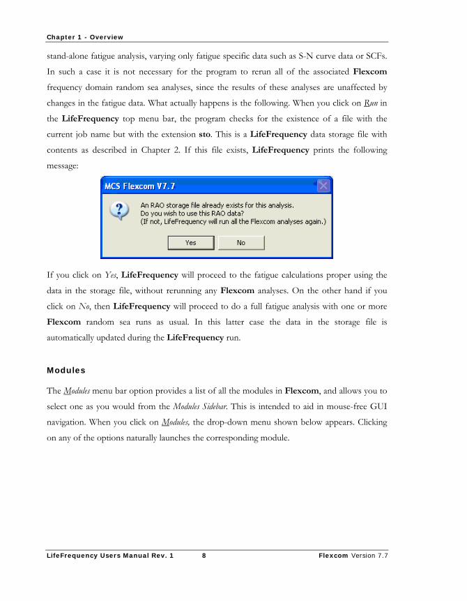
When you do run a LifeFrequency analysis, one check is performed which is specific to the
fatigue program. The section 'Repeat Runs' of Chapter 2 describes how it is possible to rerun a
Chapter 1 - Overview
LifeFrequency Users Manual Rev. 1 8 Flexcom Version 7.7
stand-alone fatigue analysis, varying only fatigue specific data such as S-N curve data or SCFs.
In such a case it is not necessary for the program to rerun all of the associated Flexcom
frequency domain random sea analyses, since the results of these analyses are unaffected by
changes in the fatigue data. What actually happens is the following. When you click on Run in
the LifeFrequency top menu bar, the program checks for the existence of a file with the
current job name but with the extension sto. This is a LifeFrequency data storage file with
contents as described in Chapter 2. If this file exists, LifeFrequency prints the following
message:
If you click on Yes, LifeFrequency will proceed to the fatigue calculations proper using the
data in the storage file, without rerunning any Flexcom analyses. On the other hand if you
click on No, then LifeFrequency will proceed to do a full fatigue analysis with one or more
Flexcom random sea runs as usual. In this latter case the data in the storage file is
automatically updated during the LifeFrequency run.
Modules
The Modules menu bar option provides a list of all the modules in Flexcom, and allows you to
select one as you would from the Modules Sidebar. This is intended to aid in mouse-free GUI
navigation. When you click on Modules, the drop-down menu shown below appears. Clicking
on any of the options naturally launches the corresponding module.

Chapter 1 - Overview
LifeFrequency Users Manual Rev. 1 9 Flexcom Version 7.7
View
The View menu bar option allows you to examine various files associated with a
LifeFrequency fatigue analysis run by opening them in the Viewer application. Viewer is
discussed in more detail in Chapter 4 of the Flexcom Reference Manual.
Table 5.1 below tabulates the various files produced in a LifeFrequency analysis.
Chapter 1 - Overview
LifeFrequency Users Manual Rev. 1 10 Flexcom Version 7.7
Table 1.1. LifeFrequency Files.
File Name Description
jobname.lf3
jobname.sea
jobname.fat
jobname.ver
jobname.lif
jobname.t01.mpt
jobname.sto
GUI data file.
Analysis input file (1) – Fatigue seastate data.
Analysis input file (2) – Remaining data.
Verification file.
Output file.
Plot file of minimum fatigue life v distance along hot spot set (nominally a timetrace plot file).
RAO storage file (for repeat Stand-alone mode analyses – see Chapter 2 for more details)
Of these seven files, four can be examined via the Viewer application. The GUI data file is
naturally opened using LifeFrequency itself. The significance of the RAO storage file was
outlined earlier; this file is for internal program use only and is not intended to be accessed by
users. The significance of the other file, the plot file, is briefly discussed here for completeness.
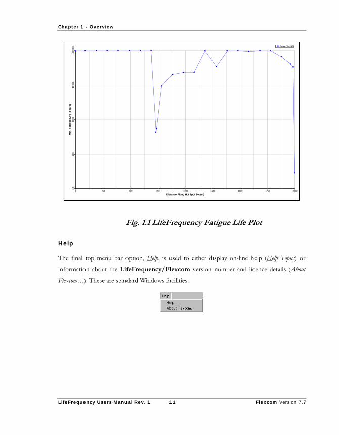
Each LifeFrequency analysis generates a plot of the minimum fatigue life at each hot spot
plotted against distance along the hot spot set. Figure 1.1 shows an example of such a fatigue
life plot. The distance on the X or horizontal axis is measured from the first element of each
hot spot set. The Y or vertical axis actually displays the fatigue life (note the logarithmic scale).
If there are two or more the user-defined hot spot sets in the fatigue run, a curve is generated
for each, and LifeFrequency automatically superimposes these curves. You can view this plot
in the usual way with the Plotting module; fatigue life plots are arbitrarily assigned the same file
extension as timetrace plots.
Chapter 1 - Overview
LifeFrequency Users Manual Rev. 1 11 Flexcom Version 7.7
0 250 500 750 1000 1250 1500 1750 2000Distance Along Hot Spot Set (m)
1010
010
0010
000
1000
00M
in. F
atig
ue L
ife (Y
ears
)
Fatigue Life - SCR
Fig. 1.1 LifeFrequency Fatigue Life Plot
Help
The final top menu bar option, Help, is used to either display on-line help (Help Topics) or
information about the LifeFrequency/Flexcom version number and licence details (About
Flexcom…). These are standard Windows facilities.


Chapter 2 - Stand-alone Operation
LifeFrequency Users Manual Rev. 1 13 Flexcom Version 7.7
CHAPTER 2 - STAND-ALONE OPERATION
This chapter provides the background to the program Stand-alone mode of operation in the
following sections:
− ‘Introduction’ gives an overview of the program Stand-alone mode.
− ‘Long Term Environmental Conditions’ describes the input of the long-term
environmental conditions, in terms of seastates and directions.
− ‘Fatigue Data’ summarises the program options for specifying data specific to the fatigue
damage calculations.
− ‘Analysis Procedure’ discusses how this data is used in performing a LifeFrequency
analysis.
− ‘Jonswap Spectrum’ describes how LifeFrequency calculates parameters for the
Jonswap spectrum.
− ‘A Note on Units’ discusses how units for forces, stresses etc. are handled by the various
components of the LifeFrequency package.
− ‘Repeat Runs’ describes how analyses can in some cases be repeated with a much-
reduced computing time.
− ‘References’ presents a number of appropriate references.
INTRODUCTION
The operation of LifeFrequency is best described by first detailing the required program
inputs, and then describing how LifeFrequency uses these inputs to produce fatigue life
estimates.
The input data required for the fatigue analysis using LifeFrequency can be grouped under
three headings or categories as follows:
Category i): Structure finite element model and general environmental data (water
depth and density, mud density, and so on).
Chapter 2 - Stand-alone Operation
LifeFrequency Users Manual Rev. 1 14 Flexcom Version 7.7
Category ii): Wave scatter diagram and long-term directionality data.
Category iii): Fatigue-specific data such as hot spot locations, stress concentration
factors and material S-N curves.
LifeFrequency reads the required data in Category (i) from a Flexcom input file. You input
and save this data via the Flexcom Analysis module, and then in the LifeFrequency GUI
you simply specify the Flexcom file name you used when saving the data. The data should
include all of the inputs you would normally specify for a Flexcom random sea analysis,
except that no wave data is required. The reason for this is explained later in this chapter.
LONG TERM ENVIRONMENTAL CONDITIONS
Wave Scatter Diagram
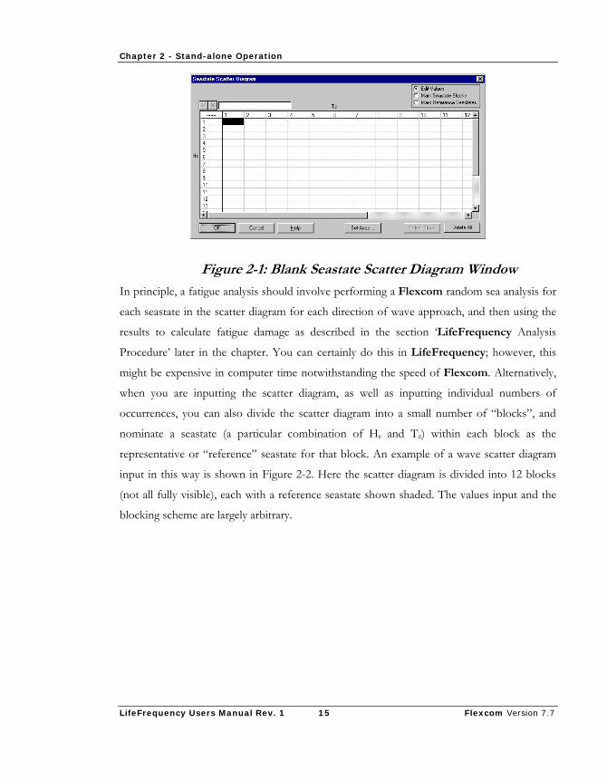
Category (ii) above relates to the long-term environmental conditions at the location in
question. The first element of this is the wave scatter diagram, which is input via a window in
the LifeFrequency GUI. A blank Seastate Scatter Diagram window is shown in Figure 2-1.
A detailed discussion of this window is provided in Chapter 4. However, it is briefly
discussed here as part of the description of the LifeFrequency theory. The window for
inputting the scatter diagram very much reflects how the actual wave scatter diagram is
usually presented. Each cell of the window represents a particular combination of Hs and Tz,
and you input into a cell the number of occurrences (typically the number of “three-hour
intervals”) of that particular combination during, say, a 10 or 20-year period. You can
alternatively specify the scatter diagram in terms of Hs and Tp, the wave spectrum peak
period.
Chapter 2 - Stand-alone Operation
LifeFrequency Users Manual Rev. 1 15 Flexcom Version 7.7
Figure 2-1: Blank Seastate Scatter Diagram Window
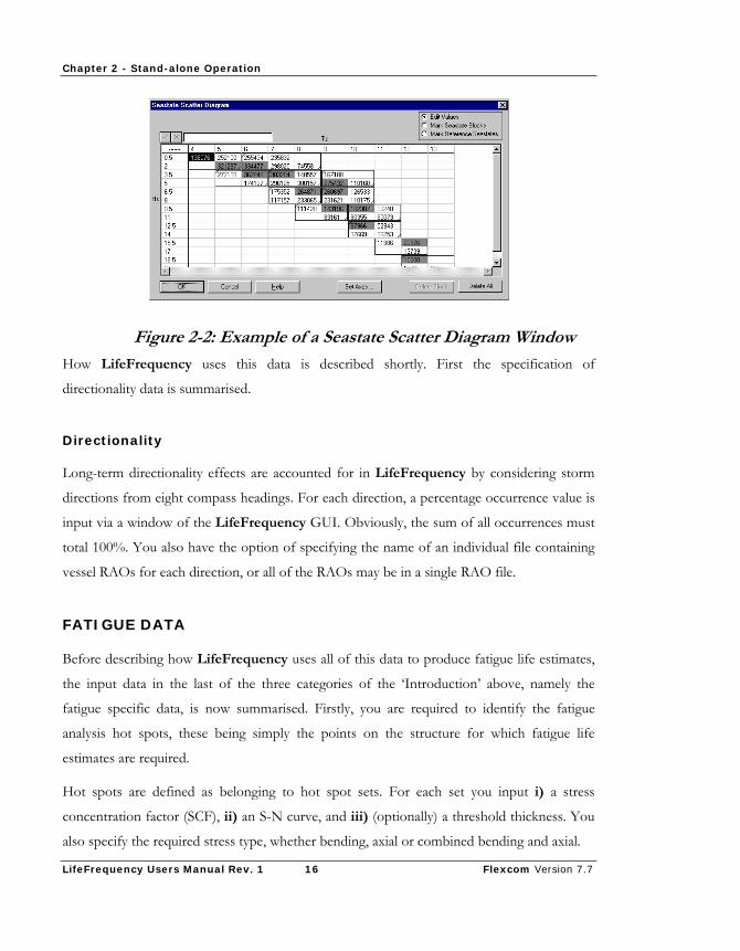
In principle, a fatigue analysis should involve performing a Flexcom random sea analysis for
each seastate in the scatter diagram for each direction of wave approach, and then using the
results to calculate fatigue damage as described in the section ‘LifeFrequency Analysis
Procedure’ later in the chapter. You can certainly do this in LifeFrequency; however, this
might be expensive in computer time notwithstanding the speed of Flexcom. Alternatively,
when you are inputting the scatter diagram, as well as inputting individual numbers of
occurrences, you can also divide the scatter diagram into a small number of “blocks”, and
nominate a seastate (a particular combination of Hs and Tz) within each block as the
representative or “reference” seastate for that block. An example of a wave scatter diagram
input in this way is shown in Figure 2-2. Here the scatter diagram is divided into 12 blocks
(not all fully visible), each with a reference seastate shown shaded. The values input and the
blocking scheme are largely arbitrary.
Chapter 2 - Stand-alone Operation
LifeFrequency Users Manual Rev. 1 16 Flexcom Version 7.7
Figure 2-2: Example of a Seastate Scatter Diagram Window
How LifeFrequency uses this data is described shortly. First the specification of
directionality data is summarised.
Directionality
Long-term directionality effects are accounted for in LifeFrequency by considering storm
directions from eight compass headings. For each direction, a percentage occurrence value is
input via a window of the LifeFrequency GUI. Obviously, the sum of all occurrences must
total 100%. You also have the option of specifying the name of an individual file containing
vessel RAOs for each direction, or all of the RAOs may be in a single RAO file.
FATIGUE DATA
Before describing how LifeFrequency uses all of this data to produce fatigue life estimates,
the input data in the last of the three categories of the ‘Introduction’ above, namely the
fatigue specific data, is now summarised. Firstly, you are required to identify the fatigue
analysis hot spots, these being simply the points on the structure for which fatigue life
estimates are required.
Hot spots are defined as belonging to hot spot sets. For each set you input i) a stress
concentration factor (SCF), ii) an S-N curve, and iii) (optionally) a threshold thickness. You
also specify the required stress type, whether bending, axial or combined bending and axial.
Chapter 2 - Stand-alone Operation
LifeFrequency Users Manual Rev. 1 17 Flexcom Version 7.7
SCF specification is standard, and the specified SCF values multiply the stresses calculated by
Flexcom/LifeFrequency to account for various stress raisers. For S-N curve specification,
a range of options is provided to allow a wide degree of generality. A particular curve may be
defined by two parameters m and K such that the curve is given by NSm = K, where S
represents stress range and N number of cycles to failure. Such a curve plots as a straight line
on log-log scales. An endurance limit (a stress range below which no fatigue damage results
regardless of the number of cycles) may be optionally specified.
Alternatively, a series of m and K values may define the curve over particular regions,
representing a piecewise-linear log-log plot. In the most general case, a particular curve may
be specified as a series of (S, N) data pairs.
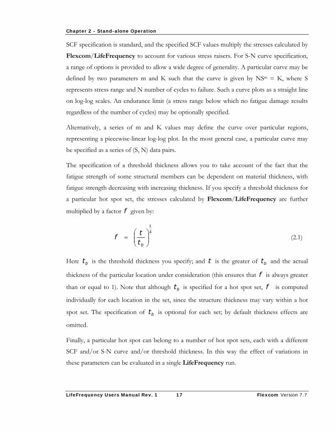
The specification of a threshold thickness allows you to take account of the fact that the
fatigue strength of some structural members can be dependent on material thickness, with
fatigue strength decreasing with increasing thickness. If you specify a threshold thickness for
a particular hot spot set, the stresses calculated by Flexcom/LifeFrequency are further
multiplied by a factor f given by:
41
⎟⎟⎠
⎞⎜⎜⎝
⎛=
btt
f (2.1)
Here bt is the threshold thickness you specify; and t is the greater of bt and the actual
thickness of the particular location under consideration (this ensures that f is always greater
than or equal to 1). Note that although bt is specified for a hot spot set, f is computed
individually for each location in the set, since the structure thickness may vary within a hot
spot set. The specification of bt is optional for each set; by default thickness effects are
omitted.
Finally, a particular hot spot can belong to a number of hot spot sets, each with a different
SCF and/or S-N curve and/or threshold thickness. In this way the effect of variations in
these parameters can be evaluated in a single LifeFrequency run.

Chapter 2 - Stand-alone Operation
LifeFrequency Users Manual Rev. 1 18 Flexcom Version 7.7
LIFEFREQUENCY ANALYSIS PROCEDURE
The rest of this chapter describes how LifeFrequency uses the data described above to
produce fatigue life estimates. A schematic of the procedure is presented in Figure 2-3.
Figure 2-3: LifeFrequency Analysis Procedure
The procedure is as follows. For every combination of i) reference seastate and ii) wave
direction with non-zero % occurrence, the program combines these seastate parameters with
the Category (i) data in the file you specified, to produce a Flexcom input file for each
combination. LifeFrequency then, without user intervention, runs each of these Flexcom
analyses, and post-processes the results to obtain stress RAOs (transfer functions). The stress
RAOs for a particular reference seastate and wave direction are then used to produce stress
spectra for all of the remaining seastates within that block for that direction. In this way stress
spectra are produced for every combination of seastate and wave direction in the long-term
Control Module
Category (i) Data
Category (ii) Data
Flexcom Input Files Analysis
ModulePost- processing
Flexcom RAO Files
Storage file (.sto)
Output file (.lif)
LifeFrequency
Category (iii) Data
Verification file (.ver)
Chapter 2 - Stand-alone Operation
LifeFrequency Users Manual Rev. 1 19 Flexcom Version 7.7
environmental data. Note that the assumption implicit in this procedure is that stress RAOs
are invariant with respect to seastate over short “distances” within the scatter diagram.
After the Flexcom analyses (including postprocessing) for each reference seastate/direction
combination have been completed, LifeFrequency proceeds to the fatigue life prediction
process proper. The fatigue life at a particular location is found by looping over all of the
seastates in the scatter diagram and all of the storm approach directions, and computing and
accumulating the fatigue damage due to each combination.
For each combination, the first step is to extract the required hot spot RAO or RAOs from
the Flexcom RAO files and to transform and/or combine these as required. The appropriate
RAO file will depend on what seastate is being analysed and what block this corresponds to
in the scatter diagram.
If you specify that combined stresses are to be considered at a particular location, then
LifeFrequency scans the Flexcom RAO output for axial force RAOs and RAOs of bending
about both local axes. The axial force RAOs are transformed to axial stress and the two
bending RAOs are transformed to bending stress. The three RAOs are then combined to
produce combined stress RAOs. The combining of the RAOs uses complex arithmetic to
include the effect of relative phasing between the stress components. Note that
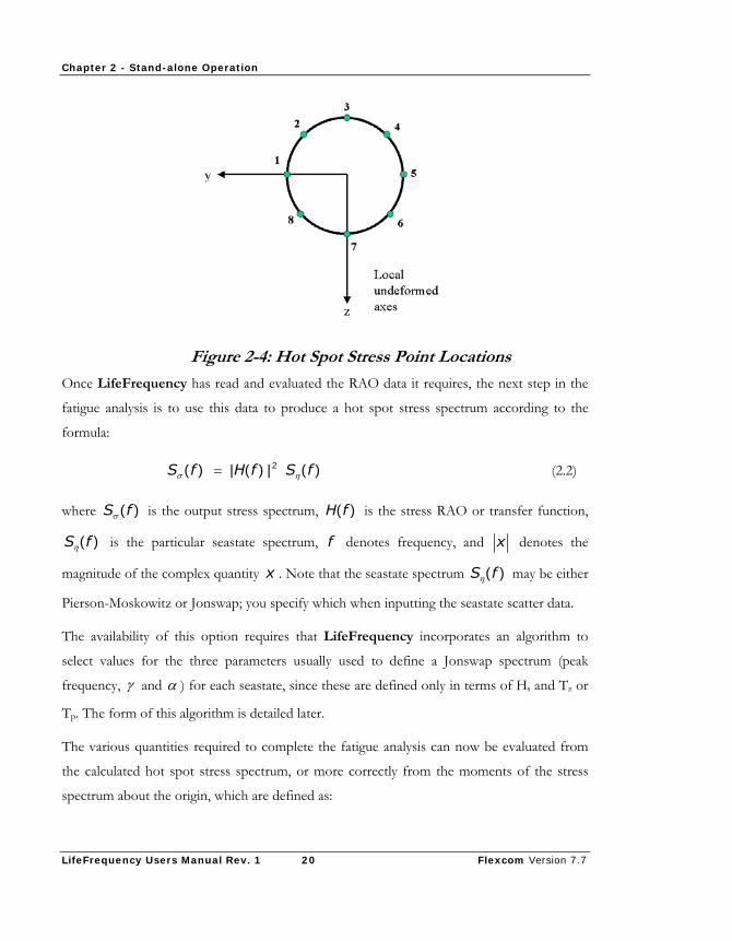
LifeFrequency produces fatigue life estimates for eight points (denoted ‘stress points’)
around the section circumference as shown in Figure 2-4, and so bending stress RAOs are
factored as appropriate depending on the actual ‘stress point’ under consideration.
Chapter 2 - Stand-alone Operation
LifeFrequency Users Manual Rev. 1 20 Flexcom Version 7.7
Figure 2-4: Hot Spot Stress Point Locations
Once LifeFrequency has read and evaluated the RAO data it requires, the next step in the
fatigue analysis is to use this data to produce a hot spot stress spectrum according to the
formula:
)(|)(|)( 2 fSfHfS ησ = (2.2)
where )(fSσ is the output stress spectrum, )(fH is the stress RAO or transfer function,
)(fSη is the particular seastate spectrum, f denotes frequency, and x denotes the
magnitude of the complex quantity x . Note that the seastate spectrum )(fSη may be either
Pierson-Moskowitz or Jonswap; you specify which when inputting the seastate scatter data.
The availability of this option requires that LifeFrequency incorporates an algorithm to
select values for the three parameters usually used to define a Jonswap spectrum (peak
frequency, γ and α ) for each seastate, since these are defined only in terms of Hs and Tz or
Tp. The form of this algorithm is detailed later.
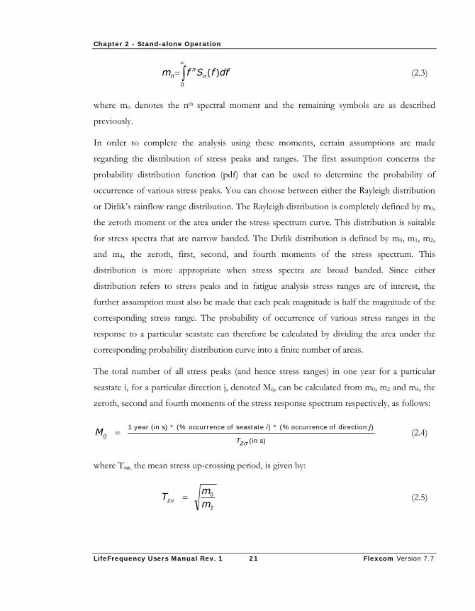
The various quantities required to complete the fatigue analysis can now be evaluated from
the calculated hot spot stress spectrum, or more correctly from the moments of the stress
spectrum about the origin, which are defined as:
Chapter 2 - Stand-alone Operation
LifeFrequency Users Manual Rev. 1 21 Flexcom Version 7.7
dffSfm nn )(
0σ∫
∞
= (2.3)
where mn denotes the nth spectral moment and the remaining symbols are as described
previously.
In order to complete the analysis using these moments, certain assumptions are made
regarding the distribution of stress peaks and ranges. The first assumption concerns the
probability distribution function (pdf) that can be used to determine the probability of
occurrence of various stress peaks. You can choose between either the Rayleigh distribution
or Dirlik’s rainflow range distribution. The Rayleigh distribution is completely defined by m0,
the zeroth moment or the area under the stress spectrum curve. This distribution is suitable
for stress spectra that are narrow banded. The Dirlik distribution is defined by m0, m1, m2,
and m4, the zeroth, first, second, and fourth moments of the stress spectrum. This
distribution is more appropriate when stress spectra are broad banded. Since either
distribution refers to stress peaks and in fatigue analysis stress ranges are of interest, the
further assumption must also be made that each peak magnitude is half the magnitude of the
corresponding stress range. The probability of occurrence of various stress ranges in the
response to a particular seastate can therefore be calculated by dividing the area under the
corresponding probability distribution curve into a finite number of areas.
The total number of all stress peaks (and hence stress ranges) in one year for a particular
seastate i, for a particular direction j, denoted Mij, can be calculated from m0, m2 and m4, the
zeroth, second and fourth moments of the stress response spectrum respectively, as follows:
)sin(
)direction ofoccurrence(%*)seastateofoccurrence(%*)sin(year1
σzT
jiijM = (2.4)
where Tzσ, the mean stress up-crossing period, is given by:
2
0
mm
Tz =σ (2.5)
Chapter 2 - Stand-alone Operation
LifeFrequency Users Manual Rev. 1 22 Flexcom Version 7.7
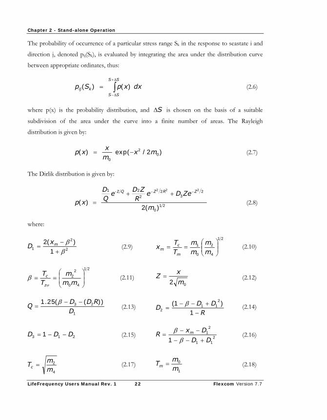
The probability of occurrence of a particular stress range Sk in the response to seastate i and
direction j, denoted pij(Sk), is evaluated by integrating the area under the distribution curve
between appropriate ordinates, thus:
∫Δ+
Δ−
=SS
SSkij dxxpSp )()( (2.6)
where p(x) is the probability distribution, and SΔ is chosen on the basis of a suitable
subdivision of the area under the curve into a finite number of areas. The Rayleigh
distribution is given by:
)2/exp()( 02
0
mxmx
xp −= (2.7)
The Dirlik distribution is given by:
21
0
23
22
2Z-1
)(2)(
222
m
ZeDeR
ZDe
QD
xp
ZRZQ −− ++= (2.8)
where:
2
2
1 1)(2
ββ
+−
= mxD (2.9)
21
4
2
0
1⎟⎟⎠
⎞⎜⎜⎝
⎛==
mm
mm
TT
xm
cm (2.10)
21
40
22
⎟⎟⎠
⎞⎜⎜⎝
⎛==
mmm
TT
z
c
σ
β (2.11) 02 m
xZ = (2.12)
1
23 ))((25.1D
RDDQ
−−=
β (2.13)
RDD
D−
+−−=
1)1( 2
112
β (2.14)
213 1 DDD −−= (2.15) 211
21
1 DD
DxR m
+−−−−
=β
β (2.16)
4
2
mm
Tc = (2.17) 1
0
mm
Tm = (2.18)
Chapter 2 - Stand-alone Operation
LifeFrequency Users Manual Rev. 1 23 Flexcom Version 7.7
The actual number of occurrences in one year of stress range Sk in response to seastate i,
direction j, denoted nij (Sk), or simply nijk, is given by:
ijkijijk MSpn )(= (2.19)
The damage due to stress range k in seastate i, direction j, as defined by the Palmgren-Miner
Rule, is found by dividing the actual number of occurrences of stress range Sk, that is nijk, by
the number of cycles of this stress range required to cause failure. This latter quantity is
denoted N(Sk) or Nk, and is found from the appropriate S-N curve. Denoting the damage
due to stress range k in seastate i, direction j, as dijk we write:
k
ijkijk N
nd = (2.20)
and the accumulated damage in the response to seastate i due to all stress ranges and
directions, denoted di, is given by:
∑∑∑∑ ==j k k
ijk
j kijki N
ndd (2.21)
The accumulated damage in one year due to all seastates, which is denoted d1, is given by:
∑=i
idd1 (2.22)
According to the Palmgren-Miner Rule the fatigue life at a particular hot spot is 1/d1 years.
This is the procedure used to predict fatigue life in LifeFrequency.
Two Special Cases
There are two special cases of the above general procedure for dividing the scatter diagram
into blocks and nominating a reference seastate within each block. Flexcom allows you to
choose these cases with a simple keyclick. The first is where you want to have only a single
block (encompassing the full scatter diagram) with a single reference seastate. In this case,
LifeFrequency does one random sea analysis only for each wave direction with non-zero %
Chapter 2 - Stand-alone Operation
LifeFrequency Users Manual Rev. 1 24 Flexcom Version 7.7
occurrence. The RAOs from these analyses are used for all of the seastates in the scatter
diagram, but otherwise the fatigue analysis proceeds exactly as per Eqs. (2.2) to (2.22).
The second special case is slightly different. In this case you want Flexcom to do a random
sea analysis for every seastate in the scatter diagram, for every wave direction with non-zero
% occurrence. This is equivalent to making every cell of the scatter diagram into both a
seastate block and the reference seastate for that block.
The fatigue life calculations are slightly different in this case to the general procedure outlined
above – but only slightly. The result of doing a Flexcom random sea analysis for every
seastate for every wave direction is that you have immediately the axial force and bending
moment spectra that are required to complete the fatigue analysis. There is no requirement in
this case to postprocess the random sea results to produce response RAOs. So in effect the
fatigue calculations begin at Eq. (2.3), the calculation of the moments of the combined stress
spectrum. Otherwise the procedure is exactly the same as in the general case.
It is important to be clear that this second special case is not LifeFrequency running in the
Postprocessor with Stress Spectra mode described in Chapter 3, although the effect is naturally
very similar. In the LifeFrequency postprocessor mode you have to run off all of the
Flexcom random sea analyses yourself before running LifeFrequency. In this second
special case of the Stand-alone mode, LifeFrequency automatically performs all of the
Flexcom runs before then proceeding directly to the fatigue life calculations.
JONSWAP SPECTRUM
The Jonswap spectrum is defined by three parameters, namely fp (peak frequency), γ
(peakedness parameter) and α (Phillips constant). When you describe a Jonswap spectrum in
terms of Hs and Tz or Hs and Tp, then LifeFrequency uses special algorithms to select
appropriate values for fp, γ and α . These are now summarised.
For the case of a scatter diagram defined as Hs/Tz combinations, the method adopted here is
one due to Isherwood [1] who publishes in his paper of 1987 a revised Jonswap spectrum
parameterisation based on empirical data published by Huomb and Overvik [2]. This
procedure will not be described in detail here; the interested reader is referred to the
Chapter 2 - Stand-alone Operation
LifeFrequency Users Manual Rev. 1 25 Flexcom Version 7.7
publications referenced, or to Flexcom Technical Note 7, ‘Alternative Jonswap Spectrum
Formulations’.
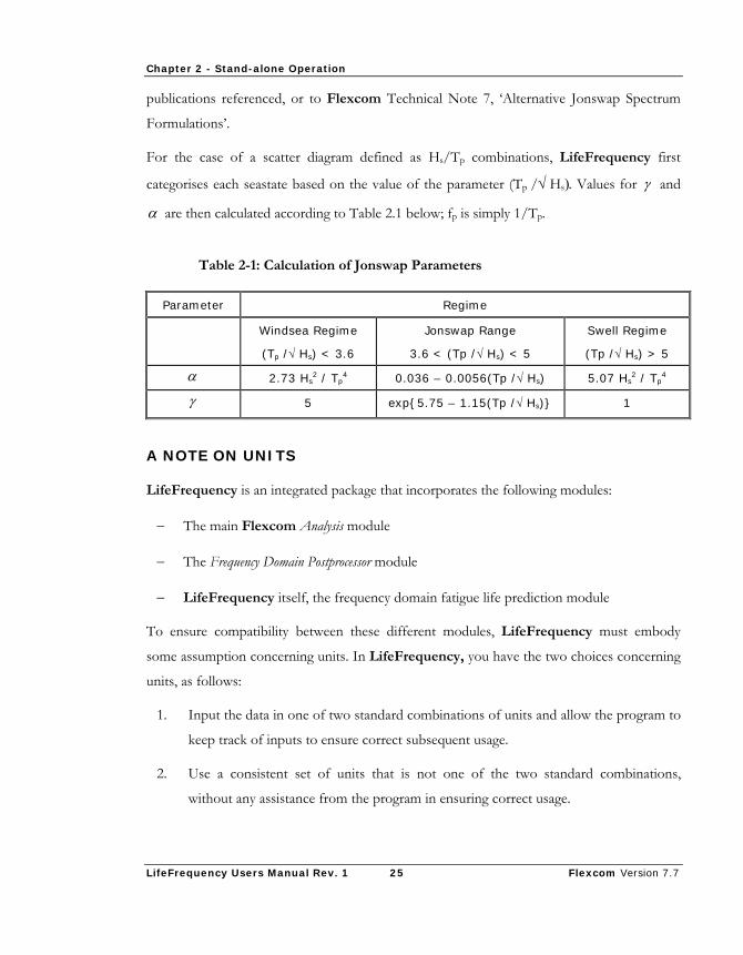
For the case of a scatter diagram defined as Hs/Tp combinations, LifeFrequency first
categorises each seastate based on the value of the parameter (Tp /√ Hs). Values for γ and
α are then calculated according to Table 2.1 below; fp is simply 1/Tp.
Table 2-1: Calculation of Jonswap Parameters
Parameter Regime
Windsea Regime
(Tp /√ Hs) < 3.6
Jonswap Range
3.6 < (Tp /√ Hs) < 5
Swell Regime
(Tp /√ Hs) > 5
α 2.73 Hs2 / Tp
4 0.036 – 0.0056(Tp /√ Hs) 5.07 Hs2 / Tp
4
γ 5 exp{5.75 – 1.15(Tp /√ Hs)} 1
A NOTE ON UNITS
LifeFrequency is an integrated package that incorporates the following modules:
− The main Flexcom Analysis module
− The Frequency Domain Postprocessor module
− LifeFrequency itself, the frequency domain fatigue life prediction module
To ensure compatibility between these different modules, LifeFrequency must embody
some assumption concerning units. In LifeFrequency, you have the two choices concerning
units, as follows:
1. Input the data in one of two standard combinations of units and allow the program to
keep track of inputs to ensure correct subsequent usage.
2. Use a consistent set of units that is not one of the two standard combinations,
without any assistance from the program in ensuring correct usage.

Chapter 2 - Stand-alone Operation
LifeFrequency Users Manual Rev. 1 26 Flexcom Version 7.7
The following are the two standard systems of units that you can use to prepare the various
LifeFrequency data files:
− SI units
Mass - kg; Length - m; Time - s
Force - N; Moment - Nm
Stress - N/mm2 (MPa) (S-N curve specification)
Value of g (gravitational constant) - 9.81m/s2
− Imperial units
Mass - slugs; Length - ft; Time - s
Force - lb (lbf); Moment - ft lb
Stress - ksi (kips/in2) (S-N curve specification)
Value of g (gravitational constant) - 32.2 ft/s2
If you specify to LifeFrequency that you are using one of these standard units sets, you do
not need to nominate which one. The program determines which set of units is being used
from the value you specify for g in inputting the Category (i) data in the Flexcom Analysis
module. This will obviously be equal to either of the above values (to within 5%), otherwise
the program will terminate with error.
REPEAT RUNS
Repeat analyses, where the structural and seastate input data remains the same, can in many
cases be carried out by LifeFrequency without the necessity of continuously performing all
of the Flexcom analyses. This is achieved through the use of a storage file generated in an
initial fatigue run. This storage file contains all the structural data and all of the RAO files
generated in postprocessing the individual Flexcom analyses. In the repeat analysis, the
required files are extracted from the storage file by LifeFrequency, and the analysis then

Chapter 2 - Stand-alone Operation
LifeFrequency Users Manual Rev. 1 27 Flexcom Version 7.7
proceeds as before. This allows you to quickly examine the effect of varying fatigue specific
data, such as SCF or S-N curve.
Note though that only RAOs are preserved in the storage file. If your fatigue analysis
approach is based on performing Flexcom random sea analyses for all seastates in the scatter
diagram (the so-called second special case above), the results of the individual Flexcom runs
are not stored for subsequent reuse (the storage file would be enormous). In fact these files
are deleted at the end of the LifeFrequency run. So if you want to repeat a fatigue analysis
of this type, LifeFrequency must rerun all of the individual Flexcom analyses.
REFERENCES
1. Isherwood, R.M., “Technical Note: A Revised Parameterisation of the Jonswap
Spectrum”, Applied Ocean Research, Vol. 9, No. 1, 1987, pp. 47-50.
2. Houmb, O.G. and Overvik, T., “Parameterisation of Wave Spectra and Long Term Joint
Distribution of Wave Height and Period”, Proceedings of Conference on Behaviour
of Offshore Structures (BOSS), Trondheim, 1976, Vol. 1.

Chapter 3 - Postprocessor with Stress Spectra Operation
LifeFrequency Users Manual Rev. 1 29 Flexcom Version 7.7
CHAPTER 3 - POSTPROCESSOR WITH STRESS
SPECTRA OPERATION
This chapter provides the background to the program Postprocessor with Stress Spectra mode of
operation in the following sections:
− ‘Introduction’ gives an overview of the program Postprocessor with Stress Spectra mode.
− ‘Operation’ details the LifeFrequency procedure in this mode.
− ‘Units’ discusses how units for forces, stresses etc. are handled in this mode.
INTRODUCTION
You run LifeFrequency in Postprocessor with Stress Spectra mode when you have yourself
performed Flexcom frequency domain random sea analyses for each combination of wave
height, wave period, and wave direction in the fatigue load case. The input to LifeFrequency
in this case is a list of Flexcom output file names, together with a % occurrence value for the
combination of conditions that each analysis considered. LifeFrequency in this case
operates as a simple postprocessor to Flexcom. This mode of operation is in contrast to the
Stand-alone mode described in Chapter 2, where LifeFrequency undertakes all stages of the
fatigue analysis directly.
A situation where you might need to run LifeFrequency as a Flexcom postprocessor is
where you want to vary environmental conditions other than just wave height, wave period
or wave direction. For example, you might want to specify different offsets for, say, near, far
and cross cases – LifeFrequency does not allow you to vary offset in this way. On the other
hand, you might want to nominate different drift conditions for different seastates. If you do,
you must run the individual Flexcom random sea analyses yourself before running
LifeFrequency in Postprocessor with Stress Spectra mode.
Chapter 3 - Postprocessor with Stress Spectra Operation
LifeFrequency Users Manual Rev. 1 30 Flexcom Version 7.7
OPERATION
The actual LifeFrequency fatigue calculations in this mode are only slightly different from
the Stand-alone mode calculations of Eqs. (2.2) to (2.21) of the previous chapter. Obviously
the result of doing a Flexcom random sea analysis for every seastate for every wave direction
is that you have immediately the axial force and bending moment spectra that are required
for the fatigue analysis. So the fatigue calculations begin at Eq. (2.3), the calculation of the
moments of the combined stress spectrum. Otherwise the procedure is exactly the same
from this point. In this regard, this postprocessor mode is very similar to the second special
case of the stand-alone mode discussed previously. This special case is where LifeFrequency
does a Flexcom analysis for every combination of wave parameters. The similarities between
the two situations are obvious.
Because you (rather than LifeFrequency) run the individual Flexcom analyses, and because
LifeFrequency is dealing directly with the stress spectra produced by these runs, there is no
need for the fatigue program to know the actual combinations of environmental conditions
corresponding to each run. The only environmental data required is the % annual occurrence
of this combination. So the dialog for inputting the LifeFrequency Postprocessor with Stress
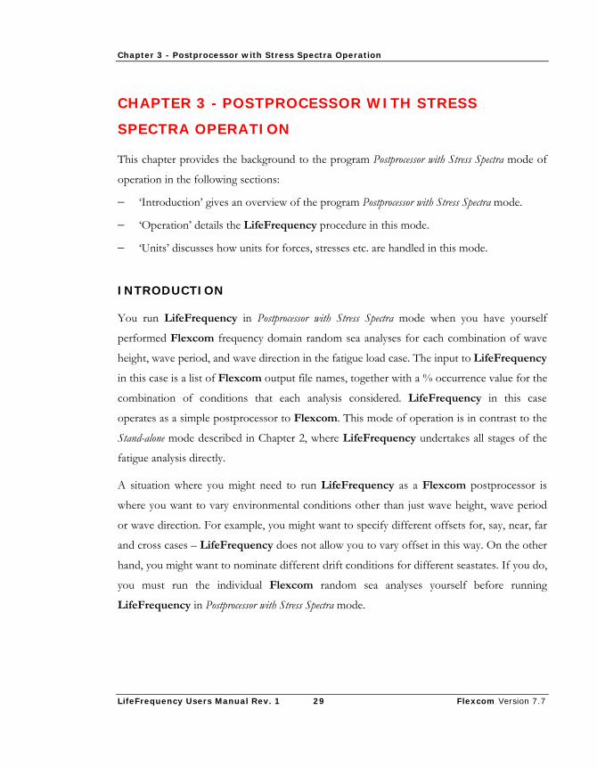
Spectra mode data is as shown below.
Figure 3-1: Pre-run Analyses Dialog
Further details about this dialog are provided in Chapter 5. The percentage value you input
here is used in a slightly amended form of Eq. (2.4), where it replaces the product “(%
occurrence of seastate i) * (% occurrence of direction j)”. The amended form of the equation is:
Chapter 3 - Postprocessor with Stress Spectra Operation
LifeFrequency Users Manual Rev. 1 31 Flexcom Version 7.7
s)(inTn)combinatiothisofoccurrence(%*s)(inyear1
zσ
=ijM (3.1)
Other than this, the fatigue calculations are exactly as described in Chapter 2.
UNITS
Chapter 2 describes how you have the option of using one of two standard systems of units
(SI or Imperial) in setting up a LifeFrequency analysis in the Stand-alone mode, and how, if
you invoke this option, the program automatically determines which system you are using
from your value for the gravitational constant g. This option is also available for the
Postprocessor with Stress Spectra mode. What happens if you invoke this facility (using Options –
Units:), is that LifeFrequency reads the value for g from the postprocessing output file
produced by the first Flexcom analysis listed in the Pre-run Analyses dialog shown above in
Figure 3-1. The assumption is that you used the same value of g in all your analyses; to do
otherwise would be unusual.
What this mainly affects in the Postprocessor with Stress Spectra mode input data is the
specification of S-N curves and SCFs. S-N curve data is usually input in units consistent with
stresses in MPa (SI units) or ksi (Imperial units). However, the axial forces and bending
moments in your Flexcom output files are typically in N and Nm (SI units) or lb and ft.lb
(Imperial units). In early versions of LifeFrequency, this meant that you typically used your
SCFs to transform stresses to units consistent with your S-N curve(s). So for example, if you
were using SI units and wanted to specify a SCF of 1.2 and stress ranges in MPa in your S-N
curve, you specified an SCF of 1.2*10-6 to ensure compatibility. Likewise for Imperial units, if
you wanted to use ksi in defining your S-N data, the SCF you specified was 1.2*6.9444*10-6
or 8.3333*10-6.
Now you can specify Automatic units, an SCF of 1.2, and your S-N curve in MPa or ksi, and
let LifeFrequency take care of ensuring consistency of units thereafter.


Chapter 4 - Postprocessor with RAOs Operation
LifeFrequency Users Manual Rev. 1 33 Flexcom Version 7.7
CHAPTER 4 - POSTPROCESSOR WITH RAOS
OPERATION
This chapter provides the background to the program Postprocessor with RAOs mode of
operation in the following sections:
− ‘Introduction’ gives an overview of the program Postprocessor with RAOs mode.
− ‘Operation’ details the LifeFrequency procedure in this mode.
− ‘Units’ discusses how units for forces, stresses etc. are handled in this mode.
INTRODUCTION
The LifeFrequency Postprocessor with RAOs mode of operation combines elements from the
other two modes described in the last two chapters. It is similar to the Stand-alone mode in
that you input the wave scatter diagram and directionality data in full, and you divide the
scatter diagram into blocks and nominate a reference seastate in each block in the same way.
What is different from the Stand-alone mode is that you must run the Flexcom frequency
domain random sea analyses yourself, before running LifeFrequency, for each combination
of reference seastate and direction with non-zero % occurrence. In this regard the Postprocessor
with RAOs mode resembles the Postprocessor with Stress Spectra mode. Even here though there is
another difference. In addition to running the Flexcom analyses, you must also postprocess
them to generate RAOs of axial force and bending moment at the locations of interest (‘hot
spots’), since LifeFrequency requires these to complete the fatigue calculations as per the
Stand-alone mode.
OPERATION
The actual LifeFrequency fatigue calculations in this mode are identical to the Stand-alone
mode calculations of Eqs. (2.2) to (2.22) of Chapter 2.
The actual data inputs you specify are also very similar to the Stand-alone mode. You specify
the wave scatter diagram and the directionality data using exactly the same dialogs as for the
Chapter 4 - Postprocessor with RAOs Operation
LifeFrequency Users Manual Rev. 1 34 Flexcom Version 7.7
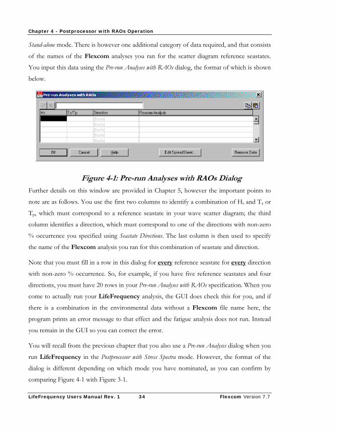
Stand-alone mode. There is however one additional category of data required, and that consists
of the names of the Flexcom analyses you ran for the scatter diagram reference seastates.
You input this data using the Pre-run Analyses with RAOs dialog, the format of which is shown
below.
Figure 4-1: Pre-run Analyses with RAOs Dialog
Further details on this window are provided in Chapter 5, however the important points to
note are as follows. You use the first two columns to identify a combination of Hs and Tz or
Tp, which must correspond to a reference seastate in your wave scatter diagram; the third
column identifies a direction, which must correspond to one of the directions with non-zero
% occurrence you specified using Seastate Directions. The last column is then used to specify
the name of the Flexcom analysis you ran for this combination of seastate and direction.
Note that you must fill in a row in this dialog for every reference seastate for every direction
with non-zero % occurrence. So, for example, if you have five reference seastates and four
directions, you must have 20 rows in your Pre-run Analyses with RAOs specification. When you
come to actually run your LifeFrequency analysis, the GUI does check this for you, and if
there is a combination in the environmental data without a Flexcom file name here, the
program prints an error message to that effect and the fatigue analysis does not run. Instead
you remain in the GUI so you can correct the error.
You will recall from the previous chapter that you also use a Pre-run Analyses dialog when you
run LifeFrequency in the Postprocessor with Stress Spectra mode. However, the format of the
dialog is different depending on which mode you have nominated, as you can confirm by
comparing Figure 4-1 with Figure 3-1.

Chapter 4 - Postprocessor with RAOs Operation
LifeFrequency Users Manual Rev. 1 35 Flexcom Version 7.7
UNITS
Chapter 2 describes how you have the option of using one of two standard systems of units
(SI or Imperial) in setting up a LifeFrequency analysis in the Stand-alone mode, and how if
you invoke this option the program automatically determines which system you are using
from your value for the gravitational constant g. This option is available for the Postprocessor
with RAOs mode as well. What happens if you invoke this option (using Options – Units:) is
that LifeFrequency reads the value for g from the data produced by the first Flexcom
analysis in your list in the Pre-run Analyses with RAOs dialog shown above in Figure 4-1. The
assumption is that you used the same value of g in all your analyses; to do otherwise would
be unusual.
What this mainly affects in the Postprocessor with RAOs mode is the postprocessing of your
Flexcom analyses. S-N curve data is usually input in units consistent with stresses in MPa (SI
units) or ksi (Imperial units). However, the axial force and bending moment RAOs in your
Flexcom RAO files are typically in N/m and Nm/m (SI units) or lb/ft and ft.lb/ft (Imperial
units). One option you could use would be to use a scale factor in your Flexcom
postprocessing to generate RAOs units consistent with your S-N curve(s). So, for example, if
you were using SI units and wanted to specify stress ranges in MPa in your S-N curve, you
could specify a postprocessing scale factor of 1*10-6 for both axial force and bending
moment RAOs. This would give RAOs in MN/m and MNm/m in your RAO file, leading to
stresses in MPa in LifeFrequency. For Imperial units, a similar procedure could apply.
However, this is not necessary. It is easier to specify a scale factor of 1 everywhere when
postprocessing; then nominate Automatic units in LifeFrequency, and let LifeFrequency
take care of ensuring consistency of units thereafter.


Chapter 5 - Reference
LifeFrequency Users Manual Rev. 1 37 Flexcom Version 7.7
CHAPTER 5 - REFERENCE
This chapter provides a detailed reference for all of the data inputs required for
LifeFrequency. It contains only a single section, ‘LifeFrequency - Reference’.


LifeFrequency – Reference

Chapter 5 - Reference
LifeFrequency Users Manual Rev. 1 40 Flexcom Version 7.7
Analysis Title
Location: LifeFrequency
Purpose: To specify a title for a LifeFrequency run.
Window:
Data Inputs:
Input: Description
Title: A title of up to 80 alphanumeric characters. This will
subsequently appear on all LifeFrequency output.
Chapter 5 - Reference
LifeFrequency Users Manual Rev. 1 41 Flexcom Version 7.7
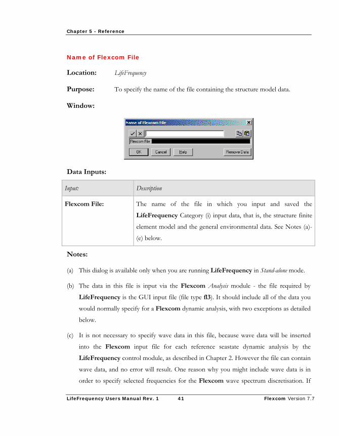
Name of Flexcom File
Location: LifeFrequency
Purpose: To specify the name of the file containing the structure model data.
Window:
Data Inputs:
Input: Description
Flexcom File: The name of the file in which you input and saved the
LifeFrequency Category (i) input data, that is, the structure finite
element model and the general environmental data. See Notes (a)-
(e) below.
Notes:
(a) This dialog is available only when you are running LifeFrequency in Stand-alone mode.
(b) The data in this file is input via the Flexcom Analysis module - the file required by
LifeFrequency is the GUI input file (file type fl3). It should include all of the data you
would normally specify for a Flexcom dynamic analysis, with two exceptions as detailed
below.
(c) It is not necessary to specify wave data in this file, because wave data will be inserted
into the Flexcom input file for each reference seastate dynamic analysis by the
LifeFrequency control module, as described in Chapter 2. However the file can contain
wave data, and no error will result. One reason why you might include wave data is in
order to specify selected frequencies for the Flexcom wave spectrum discretisation. If

Chapter 5 - Reference
LifeFrequency Users Manual Rev. 1 42 Flexcom Version 7.7
you do input random sea data with selected frequencies, the actual spectrum parameters
you specify (for example Hs and Tz for a Pierson-Moskowitz spectrum) will be ignored,
but the selected frequencies will be inserted into all the reference seastate input files by
the control module.
(d) The Flexcom file may contain data in the Vessel – RAO File dialog, but this will be
ignored by LifeFrequency. The name or names of files containing RAOs for individual
or all wave directions are required inputs in the LifeFrequency Seastate Directions dialog.
(e) The Flexcom GUI file type fl3 is not required when inputting the Flexcom file name.

Chapter 5 - Reference
LifeFrequency Users Manual Rev. 1 43 Flexcom Version 7.7
Units
Location: LifeFrequency
Purpose: To specify the units employed in inputting the LifeFrequency data.
Window:
Data Inputs: None
Notes:
(a) Chapters 2-4 describe how you can use either a pre-defined set of units or a user-defined
consistent set when inputting LifeFrequency data. You use this drop-down menu to tell
LifeFrequency the set you are using. The default is Automatic.
(b) Pre-defined units can be either SI or Imperial, as described in Chapter 2. You do not
need to specify which; LifeFrequency automatically determines this from the value you
use for g, the gravitational constant. This explains the significance of the Automatic
button.

Chapter 5 - Reference
LifeFrequency Users Manual Rev. 1 44 Flexcom Version 7.7
Location: LifeFrequency
Purpose: To specify the probability density function to be used in calculating fatigue
life estimates from stress spectra.
Window:
Data Inputs: None
Notes:
(a) This drop-down list allows the selection of the probability density function (pdf) for use
in the fatigue life calculations. Selecting Rayleigh (the default) selects the standard
Rayleigh pdf, while selecting Dirlik selects the rainflow range pdf proposed by Dirlik.
The Dirlik pdf is more appropriate when stress spectra are broad banded; the Rayleigh
pdf is narrow banded. Further details can be found in the section ‘LifeFrequency
Analysis Procedure’ in Chapter 2.
Chapter 5 - Reference
LifeFrequency Users Manual Rev. 1 45 Flexcom Version 7.7
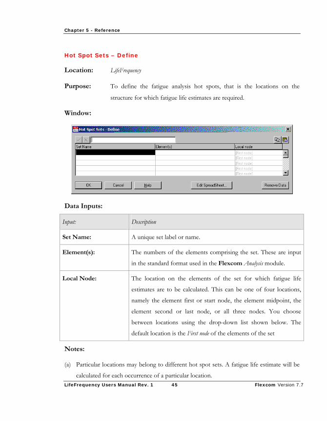
Hot Spot Sets – Define
Location: LifeFrequency
Purpose: To define the fatigue analysis hot spots, that is the locations on the
structure for which fatigue life estimates are required.
Window:
Data Inputs:
Input: Description
Set Name: A unique set label or name.
Element(s): The numbers of the elements comprising the set. These are input
in the standard format used in the Flexcom Analysis module.
Local Node: The location on the elements of the set for which fatigue life
estimates are to be calculated. This can be one of four locations,
namely the element first or start node, the element midpoint, the
element second or last node, or all three nodes. You choose
between locations using the drop-down list shown below. The
default location is the First node of the elements of the set
Notes:
(a) Particular locations may belong to different hot spot sets. A fatigue life estimate will be
calculated for each occurrence of a particular location.

Chapter 5 - Reference
LifeFrequency Users Manual Rev. 1 46 Flexcom Version 7.7
Properties – Stress
Location: LifeFrequency
Purpose: To assign effective structural properties to hot spot sets for use in
calculating bending and axial stresses.
Window:
Data Inputs:
Input: Description
Set Name: The hot spot set to which the properties are to be assigned. This
defaults to all elements.
Do: The effective outer diameter for the elements of the set. The
specification of data in this column is optional, as indeed it is for all
columns. If you do not specify a value for Do, how
LifeFrequency chooses a default depends on whether you used
the Flexible Format or the Rigid Format in inputting geometric data in
Flexcom. If you used the flexible riser format, then the default is
the drag diameter for the elements of the set. If you used the rigid
riser format, then Do here defaults to Do in the Flexcom data.
Chapter 5 - Reference
LifeFrequency Users Manual Rev. 1 47 Flexcom Version 7.7
Di: The effective internal diameter for the elements of the set. Again
this entry is optional. The default is the internal diameter specified
in your Flexcom data.
Recalculate: You use this drop-down list to indicate to LifeFrequency how
default values for A, Iyy and Izz are to be chosen if any of the
subsequent three columns are left blank.
The default value of Yes means that LifeFrequency recalculates
the parameter in question using the values you specified for Do
and/or Di. The alternative of No means LifeFrequency is to use
the same value as Flexcom did for the parameter in question,
regardless of whether you have already specified effective Do
and/or Di values for this set. See Notes (b)-(g) below.
A: The effective cross-sectional area for the elements of the set. This
entry is optional. If omitted, then how LifeFrequency chooses a
default is governed by your input in Column 4, Recalculate. See Note
(b) below.
Iyy: The second moment of area about the local y-axis for the elements
of the set. This entry is optional. If omitted, then how
LifeFrequency chooses a default is governed by your input in
Column 4, Recalculate. See Note (b) below.
Izz: The second moment of area about the local z-axis for the elements
of the set. This entry is optional. If omitted, then how
LifeFrequency chooses a default is governed by your input in
Column 4, Recalculate. See Note (b) below.
Notes:
(a) The purpose of this menu is to input values to be used in calculating stresses, both
bending and axial, during a LifeFrequency analysis.
Chapter 5 - Reference
LifeFrequency Users Manual Rev. 1 48 Flexcom Version 7.7
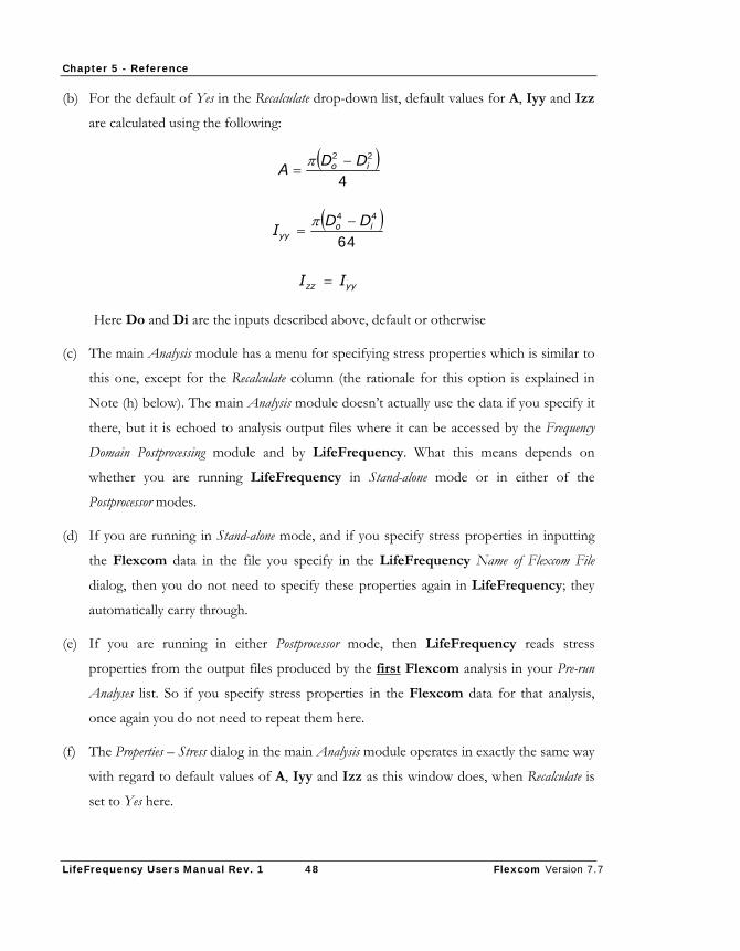
(b) For the default of Yes in the Recalculate drop-down list, default values for A, Iyy and Izz
are calculated using the following:
( )4
22io DD
A−
=π
( )64
44io
yyDD
I−
=π
yyzz II =
Here Do and Di are the inputs described above, default or otherwise
(c) The main Analysis module has a menu for specifying stress properties which is similar to
this one, except for the Recalculate column (the rationale for this option is explained in
Note (h) below). The main Analysis module doesn’t actually use the data if you specify it
there, but it is echoed to analysis output files where it can be accessed by the Frequency
Domain Postprocessing module and by LifeFrequency. What this means depends on
whether you are running LifeFrequency in Stand-alone mode or in either of the
Postprocessor modes.
(d) If you are running in Stand-alone mode, and if you specify stress properties in inputting
the Flexcom data in the file you specify in the LifeFrequency Name of Flexcom File
dialog, then you do not need to specify these properties again in LifeFrequency; they
automatically carry through.
(e) If you are running in either Postprocessor mode, then LifeFrequency reads stress
properties from the output files produced by the first Flexcom analysis in your Pre-run
Analyses list. So if you specify stress properties in the Flexcom data for that analysis,
once again you do not need to repeat them here.
(f) The Properties – Stress dialog in the main Analysis module operates in exactly the same way
with regard to default values of A, Iyy and Izz as this window does, when Recalculate is
set to Yes here.
Chapter 5 - Reference
LifeFrequency Users Manual Rev. 1 49 Flexcom Version 7.7
(g) The rationale for the two Recalculate options is as follows. This Properties – Stress facility
was introduced in a more recent version of the software. Prior to that, you only had an
option to specify an effective external diameter Do in a Diameter column on the Fatigue
Data – Properties dialog. If you did invoke the option to change Do, then LifeFrequency
did not recalculate A, Iyy and Izz; so you had in fact no facility to vary these values.
The No option on the Recalculate drop-down list is provided to allow users of a previous
version of LifeFrequency to repeat exactly the fatigue analyses run with that version.
For example, to repeat exactly a LifeFrequency Version 4.1 fatigue analysis in which
you specified a Do value for a hot spot set, you invoke this window, specify Do, and set
Recalculate to No. The hot spot stress properties should then be identical to previously.
Chapter 5 - Reference
LifeFrequency Users Manual Rev. 1 50 Flexcom Version 7.7
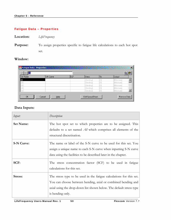
Fatigue Data – Properties
Location: LifeFrequency
Purpose: To assign properties specific to fatigue life calculations to each hot spot
set.
Window:
Data Inputs:
Input: Description
Set Name: The hot spot set to which properties are to be assigned. This
defaults to a set named All which comprises all elements of the
structural discretisation.
S-N Curve: The name or label of the S-N curve to be used for this set. You
assign a unique name to each S-N curve when inputting S-N curve
data using the facilities to be described later in the chapter.
SCF: The stress concentration factor (SCF) to be used in fatigue
calculations for this set.
Stress: The stress type to be used in the fatigue calculations for this set.
You can choose between bending, axial or combined bending and
axial using the drop-down list shown below. The default stress type
is bending only.
Chapter 5 - Reference
LifeFrequency Users Manual Rev. 1 51 Flexcom Version 7.7
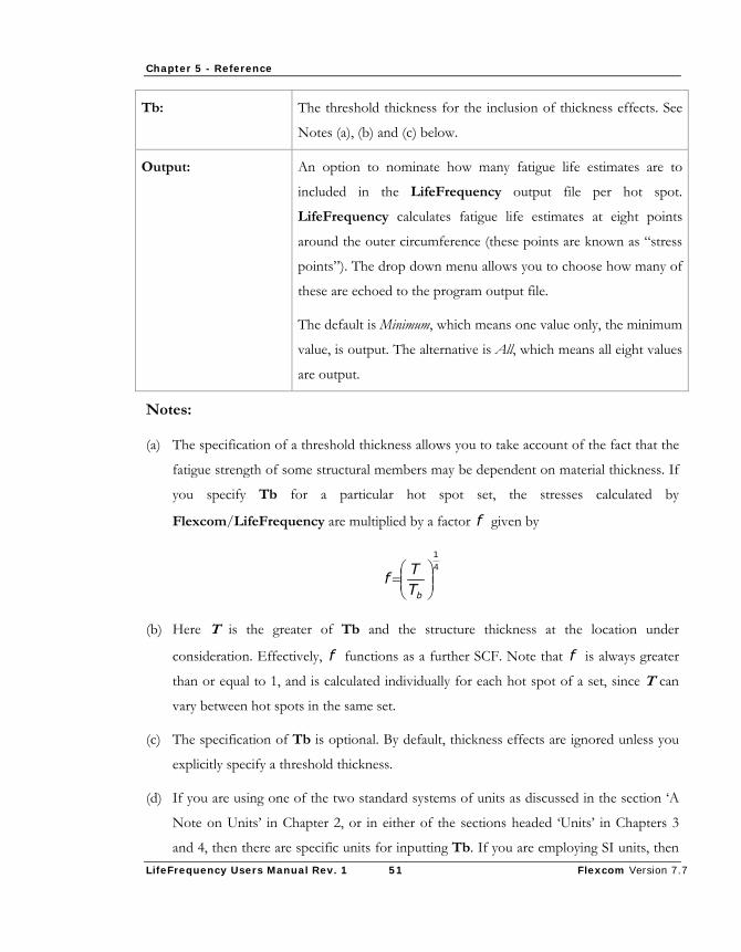
Tb: The threshold thickness for the inclusion of thickness effects. See
Notes (a), (b) and (c) below.
Output: An option to nominate how many fatigue life estimates are to
included in the LifeFrequency output file per hot spot.
LifeFrequency calculates fatigue life estimates at eight points
around the outer circumference (these points are known as “stress
points”). The drop down menu allows you to choose how many of
these are echoed to the program output file.
The default is Minimum, which means one value only, the minimum
value, is output. The alternative is All, which means all eight values
are output.
Notes:
(a) The specification of a threshold thickness allows you to take account of the fact that the
fatigue strength of some structural members may be dependent on material thickness. If
you specify Tb for a particular hot spot set, the stresses calculated by
Flexcom/LifeFrequency are multiplied by a factor f given by
41
⎟⎟⎠
⎞⎜⎜⎝
⎛=
bTT
f
(b) Here T is the greater of Tb and the structure thickness at the location under
consideration. Effectively, f functions as a further SCF. Note that f is always greater
than or equal to 1, and is calculated individually for each hot spot of a set, since T can
vary between hot spots in the same set.
(c) The specification of Tb is optional. By default, thickness effects are ignored unless you
explicitly specify a threshold thickness.
(d) If you are using one of the two standard systems of units as discussed in the section ‘A
Note on Units’ in Chapter 2, or in either of the sections headed ‘Units’ in Chapters 3
and 4, then there are specific units for inputting Tb. If you are employing SI units, then
Chapter 5 - Reference
LifeFrequency Users Manual Rev. 1 52 Flexcom Version 7.7
Tb is input in mm. If you are using Imperial units, the Tb is input in inches. If on the
other hand you are using a consistent , “User Defined” set of units then you must input
Tb in the same unit of length you used, for example, in defining nodal coordinates in the
Flexcom input data.
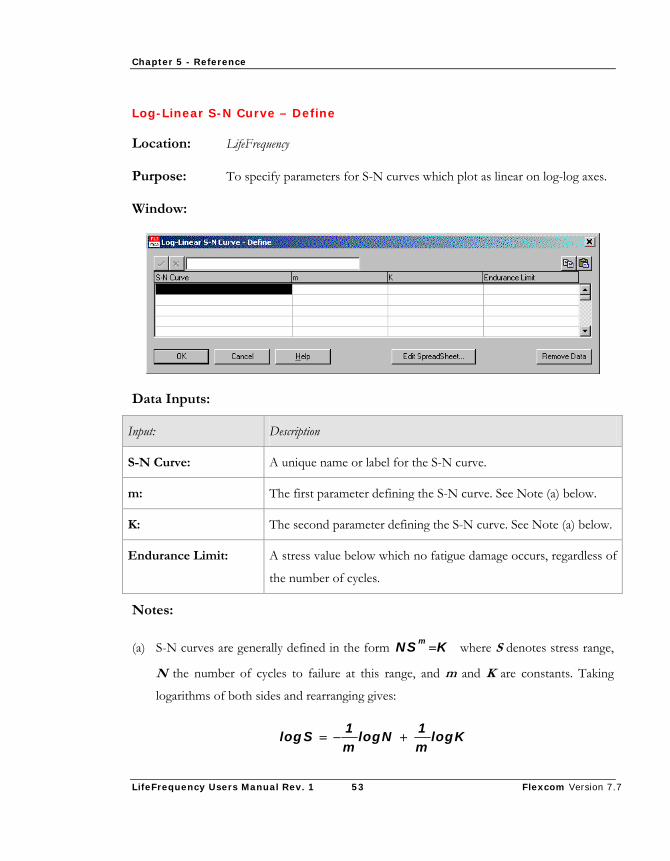
Chapter 5 - Reference
LifeFrequency Users Manual Rev. 1 53 Flexcom Version 7.7
Log-Linear S-N Curve – Define
Location: LifeFrequency
Purpose: To specify parameters for S-N curves which plot as linear on log-log axes.
Window:
Data Inputs:
Input: Description
S-N Curve: A unique name or label for the S-N curve.
m: The first parameter defining the S-N curve. See Note (a) below.
K: The second parameter defining the S-N curve. See Note (a) below.
Endurance Limit: A stress value below which no fatigue damage occurs, regardless of
the number of cycles.
Notes:
(a) S-N curves are generally defined in the form KNS m = where S denotes stress range,
N the number of cycles to failure at this range, and m and K are constants. Taking
logarithms of both sides and rearranging gives:
Klogm1
Nlogm1
Slog +−=

Chapter 5 - Reference
LifeFrequency Users Manual Rev. 1 54 Flexcom Version 7.7
which is the equation of a straight line when log S is plotted against log N. In this case
m is the inverse slope and K is a function of the line intercept. These are the parameters
input above.

Chapter 5 - Reference
LifeFrequency Users Manual Rev. 1 55 Flexcom Version 7.7
Piecewise Log-Linear S-N Curve – Define
Location: LifeFrequency
Purpose: To specify parameters for S-N curves which plot as piecewise linear
segments on log-log axes.
Window:
Data Inputs:
Input: Description
S-N Curve: A unique name or label for the S-N curve.
m: The first parameter defining the S-N curve segment. See Note (a)
below.
K: The second parameter defining the S-N curve segment. See Note
(a) below.
N1: The number of cycles value defining the lower end of the line
segment where these m and K values apply.
N2: The number of cycles value defining the upper end of the line
segment where these m and K values apply.
Chapter 5 - Reference
LifeFrequency Users Manual Rev. 1 56 Flexcom Version 7.7
Notes:
(a) This window is used to input S-N curve data when the S-N curve plots as a series of line
segments on log-log axes. In this case, particular combinations of m and K define the
curve over regions defined in terms of the N values at either end.
(b) Use as many lines as you need to completely define the S-N curve. Simply leave Column
1 blank for second and subsequent lines. For subsequent curves, put the new S-N curve
name in Column 1 and specify the curve data in the same way.
(c) When you use this specification, LifeFrequency automatically checks to ensure that the
specified S-N curve is continuous from region to region, that is, that there are no gaps or
discontinuities at the changeover points between curve regions. The presence of such a
gap will cause LifeFrequency to terminate with error.
(d) You should be careful when using this option that the S-N curve is defined over the
complete range of values likely to be of importance in a particular analysis. Note
especially that at the high cycle end of the curve, no fatigue damage is assumed to occur
at stress ranges below the minimum value specified. In effect this represents a fatigue
endurance limit.
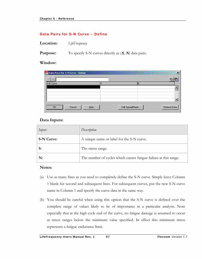
Chapter 5 - Reference
LifeFrequency Users Manual Rev. 1 57 Flexcom Version 7.7
Data Pairs for S-N Curve – Define
Location: LifeFrequency
Purpose: To specify S-N curves directly as (S, N) data pairs.
Window:
Data Inputs:
Input: Description
S-N Curve: A unique name or label for the S-N curve.
S: The stress range.
N: The number of cycles which causes fatigue failure at this range.
Notes:
(a) Use as many lines as you need to completely define the S-N curve. Simply leave Column
1 blank for second and subsequent lines. For subsequent curves, put the new S-N curve
name in Column 1 and specify the curve data in the same way.
(b) You should be careful when using this option that the S-N curve is defined over the
complete range of values likely to be of importance in a particular analysis. Note
especially that at the high cycle end of the curve, no fatigue damage is assumed to occur
at stress ranges below the minimum value specified. In effect this minimum stress
represents a fatigue endurance limit.
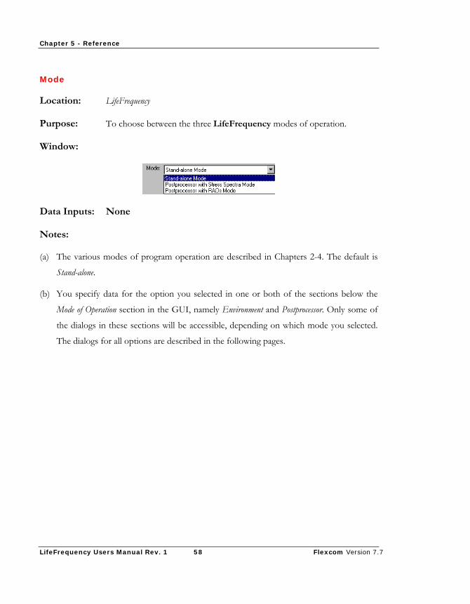
Chapter 5 - Reference
LifeFrequency Users Manual Rev. 1 58 Flexcom Version 7.7
Mode
Location: LifeFrequency
Purpose: To choose between the three LifeFrequency modes of operation.
Window:
Data Inputs: None
Notes:
(a) The various modes of program operation are described in Chapters 2-4. The default is
Stand-alone.
(b) You specify data for the option you selected in one or both of the sections below the
Mode of Operation section in the GUI, namely Environment and Postprocessor. Only some of
the dialogs in these sections will be accessible, depending on which mode you selected.
The dialogs for all options are described in the following pages.

Chapter 5 - Reference
LifeFrequency Users Manual Rev. 1 59 Flexcom Version 7.7
Seastates
Location: LifeFrequency
Purpose: To choose between formats for inputting the seastate scatter diagram in
Stand-alone and Postprocessor with Stress RAOs modes.
Window:
Data Inputs: None
Notes:
(a) The options for inputting the fatigue analysis scatter diagram are discussed in Chapter 2,
‘Stand-alone Operation’. The Selected Seastates format is the most general case, and the
other two options correspond to the ‘Two Special Cases’ discussed in Chapter 2. The
options are in fact more or less self-explanatory.
(b) To specify the actual scatter diagram data you use the Seastate Scatter Diagram dialog. The
format this dialog takes depends naturally on which of the options you choose here. The
various formats are described on the following pages. Because as it is the most general
case, the format for the Selected Seastates option is described first. The formats for the
others are variations on this general case, and are described after it.
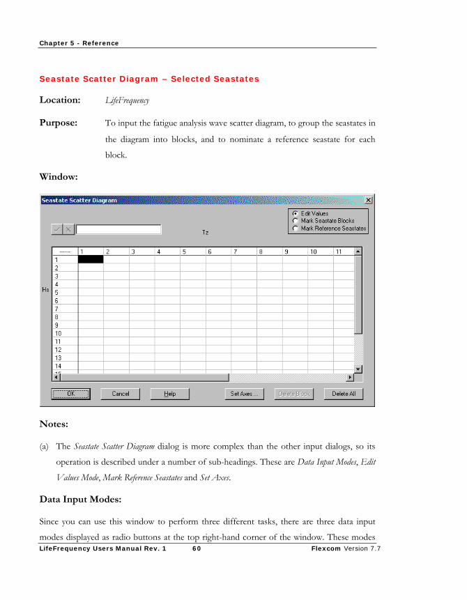
Chapter 5 - Reference
LifeFrequency Users Manual Rev. 1 60 Flexcom Version 7.7
Seastate Scatter Diagram – Selected Seastates
Location: LifeFrequency
Purpose: To input the fatigue analysis wave scatter diagram, to group the seastates in
the diagram into blocks, and to nominate a reference seastate for each
block.
Window:
Notes:
(a) The Seastate Scatter Diagram dialog is more complex than the other input dialogs, so its
operation is described under a number of sub-headings. These are Data Input Modes, Edit
Values Mode, Mark Reference Seastates and Set Axes.
Data Input Modes:
Since you can use this window to perform three different tasks, there are three data input
modes displayed as radio buttons at the top right-hand corner of the window. These modes
Chapter 5 - Reference
LifeFrequency Users Manual Rev. 1 61 Flexcom Version 7.7
are called Edit Values, Mark Seastate Blocks and Mark Reference Seastates. What happens when
you choose each of these modes is described below. There are also a number of facilities
specific to this window, which are available along the bottom of the window (in addition to
the usual ones of OK, Cancel and Help). These facilities are also described in the following
sections.
Note that by default the scatter diagram is defined in terms of significant wave height Hs and
mean zero up-crossing period Tz. How to change this to Hs and wave spectrum peak period
Tp is also described shortly.
Edit Values Mode:
The Edit Values mode is used to input and/or change (edit) the individual entries in the
scatter diagram “cells”. You simply input into each cell the number of occurrences in a given
period of the particular combination of Hs and Tz/Tp values which that cell represents. This
given period is typically one year, but the duration is in fact immaterial - LifeFrequency
transforms the data you specify into percentage occurrence values, so it is the relative
magnitudes only of the entries that are of importance. You do not have to input a value into
all cells. If there is no occurrence of a particular combination of Hs and Tz/Tp, simply leave
the corresponding cell blank.
The Delete All button at the bottom of the window can be used in Edit Values mode to clear
all cells in the scatter diagram of data. You are prompted to confirm your request to delete all
entries to prevent accidental loss of data.
Mark Seastate Blocks:
The Mark Seastate Blocks mode is used, as its name implies, to group seastates into blocks, as
described previously in Chapter 2. This task can be performed at any stage during the input
of the scatter diagram data, but would typically be performed after all of the Hs/Tz or Hs/Tp
data has been input in Edit Values mode.
When you click on the Mark Seastate Blocks button, a rectangular cursor with a diagonal line
( ) appears on the screen. You simply move this cursor to one corner of the block you
want to define, and press the left hand mouse button. Then you drag the cursor to the cell on

Chapter 5 - Reference
LifeFrequency Users Manual Rev. 1 62 Flexcom Version 7.7
the corner of the block, which is diagonally opposite the first cell, and release the mouse
button. The block you have defined will be surrounded by a thin black border, as for example
here.
Here a block has been defined with 15 seastates, with Hs values between 3 and 7 and Tz
values between 4 and 6 seconds inclusive.
If you click anywhere in an already defined seastate block when you are in Mark Seastate Block
mode that block becomes highlighted (the border around the block changes colour), and the
Delete Block button at the bottom of the window becomes active. (This facility is grey in the
pictures above, indicating that it is inactive or presently unavailable.) If you click on Delete
Block, the block border disappears, but the individual entries in the scatter diagram are
unaffected. This facility allows you to change the way in which seastates are grouped in
blocks without inputting the scatter diagram again in full.
The Delete All button at the bottom of the window can be used in Mark Seastate Blocks mode
to remove all block definitions, again without affecting the individual entries in the scatter

Chapter 5 - Reference
LifeFrequency Users Manual Rev. 1 63 Flexcom Version 7.7
diagram cells. You are prompted to confirm your request to delete all blocks to prevent
accidental loss of data.
Mark Reference Seastates:
The Mark Reference Seastates mode is used, as its name implies, to nominate reference seastates
within each block, as again described previously in Chapter 2. This task can only be
performed after one or more seastate blocks have been defined.
When you click on the Mark Reference Seastates button, a circular cursor appears on the
screen ( ). You simply move this cursor to the cell which you want to nominate as the
reference seastate and click the mouse button. The cell nominated becomes shaded, as shown
in the figure below. Here a seastate with a Hs of 2 and a Tz of 5 seconds has been nominated
as the reference seastate for a block centred on that combination.
If you click on a seastate in a block where a reference seastate is already nominated, the
previous nomination becomes deselected.
The Delete All button at the bottom of the window can be used in Mark Reference Seastates
mode to remove all reference seastate definitions, again without affecting the individual
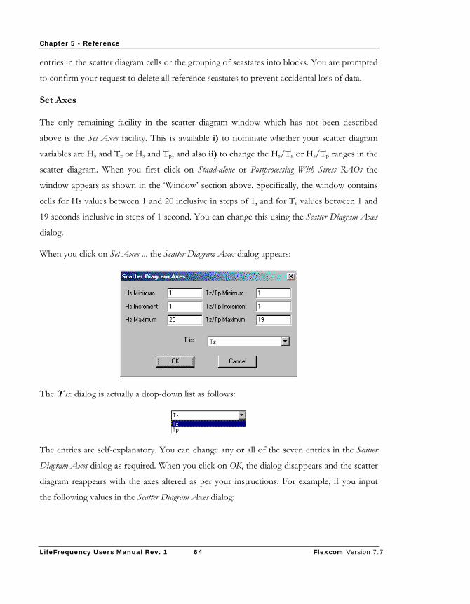
Chapter 5 - Reference
LifeFrequency Users Manual Rev. 1 64 Flexcom Version 7.7
entries in the scatter diagram cells or the grouping of seastates into blocks. You are prompted
to confirm your request to delete all reference seastates to prevent accidental loss of data.
Set Axes
The only remaining facility in the scatter diagram window which has not been described
above is the Set Axes facility. This is available i) to nominate whether your scatter diagram
variables are Hs and Tz or Hs and Tp, and also ii) to change the Hs/Tz or Hs/Tp ranges in the
scatter diagram. When you first click on Stand-alone or Postprocessing With Stress RAOs the
window appears as shown in the ‘Window’ section above. Specifically, the window contains
cells for Hs values between 1 and 20 inclusive in steps of 1, and for Tz values between 1 and
19 seconds inclusive in steps of 1 second. You can change this using the Scatter Diagram Axes
dialog.
When you click on Set Axes ... the Scatter Diagram Axes dialog appears:
The T is: dialog is actually a drop-down list as follows:
The entries are self-explanatory. You can change any or all of the seven entries in the Scatter
Diagram Axes dialog as required. When you click on OK, the dialog disappears and the scatter
diagram reappears with the axes altered as per your instructions. For example, if you input
the following values in the Scatter Diagram Axes dialog:

Chapter 5 - Reference
LifeFrequency Users Manual Rev. 1 65 Flexcom Version 7.7
then the default scatter diagram changes to the following:
It is strongly recommended that you use this facility only before inputting any data into a
scatter diagram, otherwise loss of data may occur.

Chapter 5 - Reference
LifeFrequency Users Manual Rev. 1 66 Flexcom Version 7.7
Seastate Scatter Diagram – One Seastate
Location: LifeFrequency
Purpose: To input the fatigue analysis wave scatter diagram as a single block, and to
nominate a reference seastate for that block.
Window:
Notes:
(b) This dialog is clearly very similar to that for the Selected Seastates option, and in fact differs
from it in only one respect. As you can see, the Mark Seastate Blocks option is disabled
and unavailable. This is because the entire scatter diagram constitutes a single block in
this case. Except for this one difference, this dialog is otherwise identical to the Seastate
Scatter Diagram – Selected Seastates dialog.
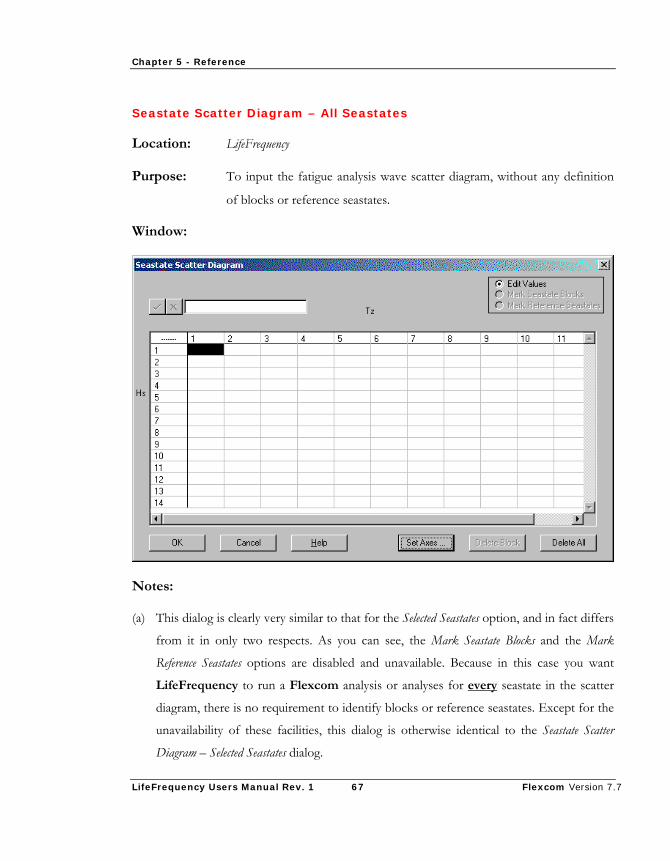
Chapter 5 - Reference
LifeFrequency Users Manual Rev. 1 67 Flexcom Version 7.7
Seastate Scatter Diagram – All Seastates
Location: LifeFrequency
Purpose: To input the fatigue analysis wave scatter diagram, without any definition
of blocks or reference seastates.
Window:
Notes:
(a) This dialog is clearly very similar to that for the Selected Seastates option, and in fact differs
from it in only two respects. As you can see, the Mark Seastate Blocks and the Mark
Reference Seastates options are disabled and unavailable. Because in this case you want
LifeFrequency to run a Flexcom analysis or analyses for every seastate in the scatter
diagram, there is no requirement to identify blocks or reference seastates. Except for the
unavailability of these facilities, this dialog is otherwise identical to the Seastate Scatter
Diagram – Selected Seastates dialog.
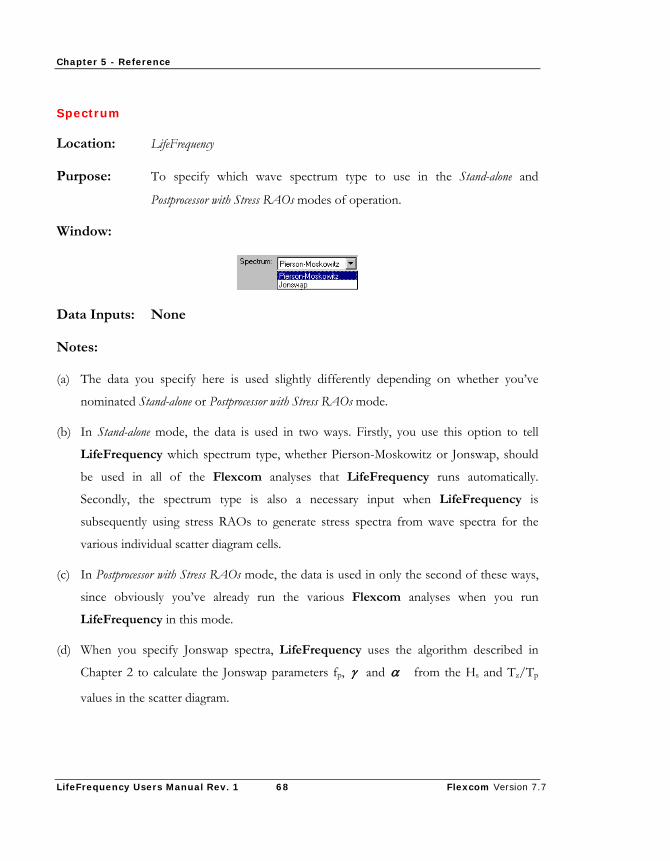
Chapter 5 - Reference
LifeFrequency Users Manual Rev. 1 68 Flexcom Version 7.7
Spectrum
Location: LifeFrequency
Purpose: To specify which wave spectrum type to use in the Stand-alone and
Postprocessor with Stress RAOs modes of operation.
Window:
Data Inputs: None
Notes:
(a) The data you specify here is used slightly differently depending on whether you’ve
nominated Stand-alone or Postprocessor with Stress RAOs mode.
(b) In Stand-alone mode, the data is used in two ways. Firstly, you use this option to tell
LifeFrequency which spectrum type, whether Pierson-Moskowitz or Jonswap, should
be used in all of the Flexcom analyses that LifeFrequency runs automatically.
Secondly, the spectrum type is also a necessary input when LifeFrequency is
subsequently using stress RAOs to generate stress spectra from wave spectra for the
various individual scatter diagram cells.
(c) In Postprocessor with Stress RAOs mode, the data is used in only the second of these ways,
since obviously you’ve already run the various Flexcom analyses when you run
LifeFrequency in this mode.
(d) When you specify Jonswap spectra, LifeFrequency uses the algorithm described in
Chapter 2 to calculate the Jonswap parameters fp, γ and α from the Hs and Tz/Tp
values in the scatter diagram.

Chapter 5 - Reference
LifeFrequency Users Manual Rev. 1 69 Flexcom Version 7.7
Seastate Directions – Stand-alone Mode
Location: LifeFrequency
Purpose: To specify long-term directionality data for the Stand-alone mode.
Window:
Data Inputs:
Input: Description
Direction: One of eight compass directions. The data in this column cannot
actually be altered. See Notes (a) and (b) below.
% Annual Occurrence: The percentage of 1 year during which storms occur from this
direction. See Notes (b) and (c) below.
RAO File Name: The name of the file containing the vessel RAOs for this direction.
See Notes (d) and (e) below.
Notes:
(a) “North” is defined as being the direction of the positive sense of the global Y axis.
“West” is then in the direction of the positive sense of the global Z axis, “South” in the
negative sense of global Y, and “East” in the negative sense of global Z. The other
directions are naturally intermediate to these.
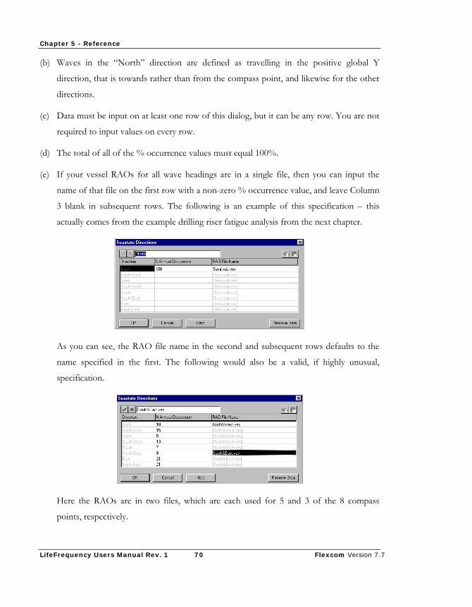
Chapter 5 - Reference
LifeFrequency Users Manual Rev. 1 70 Flexcom Version 7.7
(b) Waves in the “North” direction are defined as travelling in the positive global Y
direction, that is towards rather than from the compass point, and likewise for the other
directions.
(c) Data must be input on at least one row of this dialog, but it can be any row. You are not
required to input values on every row.
(d) The total of all of the % occurrence values must equal 100%.
(e) If your vessel RAOs for all wave headings are in a single file, then you can input the
name of that file on the first row with a non-zero % occurrence value, and leave Column
3 blank in subsequent rows. The following is an example of this specification – this
actually comes from the example drilling riser fatigue analysis from the next chapter.
As you can see, the RAO file name in the second and subsequent rows defaults to the
name specified in the first. The following would also be a valid, if highly unusual,
specification.
Here the RAOs are in two files, which are each used for 5 and 3 of the 8 compass
points, respectively.

Chapter 5 - Reference
LifeFrequency Users Manual Rev. 1 71 Flexcom Version 7.7
(f) The way in which LifeFrequency uses this data is described in Chapter 2 in the section
‘Analysis Procedure’, but is summarised here for convenience. In the other dialogs of the
Stand-alone section of the GUI, you will have identified one or more reference seastates
(and each individual seastate in the scatter diagram may be a reference seastate).
LifeFrequency creates a Flexcom input file for each combination of i) reference
seastate and ii) direction in this dialog with non-zero % occurrence. The data in the
input file comes from three sources. The structure and general environment data comes
from the Flexcom file you specify in the Name of Flexcom File dialog. The RAO data
comes from the file in Column 3 of this dialog, in the row appropriate to the direction in
question. Finally the wave data comes from both the scatter diagram (Hs and Tz/Tp) and
from this dialog (wave direction).
(g) For example, in one of the fatigue load cases in the example drilling riser analysis of the
next chapter, the scatter diagram contains 12 blocks, and there are non-zero %
occurrence values for each of the eight compass directions in this Seastate Directions
dialog. So LifeFrequency automatically generates 12*8 = 96 individual Flexcom
random sea analysis input files, runs these in turn, postprocesses each one to extract the
required response RAOs, and finally computes the actual fatigue damage for all of the
seastates in the scatter diagram as described in Chapter 2.
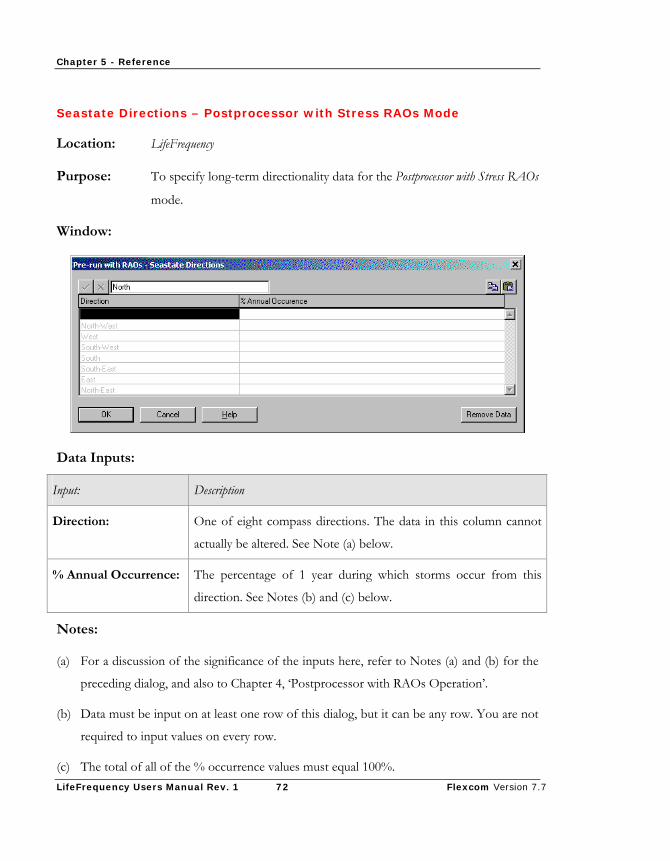
Chapter 5 - Reference
LifeFrequency Users Manual Rev. 1 72 Flexcom Version 7.7
Seastate Directions – Postprocessor with Stress RAOs Mode
Location: LifeFrequency
Purpose: To specify long-term directionality data for the Postprocessor with Stress RAOs
mode.
Window:
Data Inputs:
Input: Description
Direction: One of eight compass directions. The data in this column cannot
actually be altered. See Note (a) below.
% Annual Occurrence: The percentage of 1 year during which storms occur from this
direction. See Notes (b) and (c) below.
Notes:
(a) For a discussion of the significance of the inputs here, refer to Notes (a) and (b) for the
preceding dialog, and also to Chapter 4, ‘Postprocessor with RAOs Operation’.
(b) Data must be input on at least one row of this dialog, but it can be any row. You are not
required to input values on every row.
(c) The total of all of the % occurrence values must equal 100%.
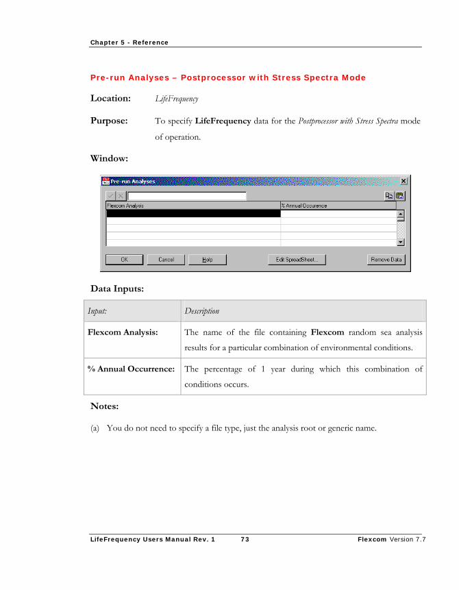
Chapter 5 - Reference
LifeFrequency Users Manual Rev. 1 73 Flexcom Version 7.7
Pre-run Analyses – Postprocessor with Stress Spectra Mode
Location: LifeFrequency
Purpose: To specify LifeFrequency data for the Postprocessor with Stress Spectra mode
of operation.
Window:
Data Inputs:
Input: Description
Flexcom Analysis: The name of the file containing Flexcom random sea analysis
results for a particular combination of environmental conditions.
% Annual Occurrence: The percentage of 1 year during which this combination of
conditions occurs.
Notes:
(a) You do not need to specify a file type, just the analysis root or generic name.
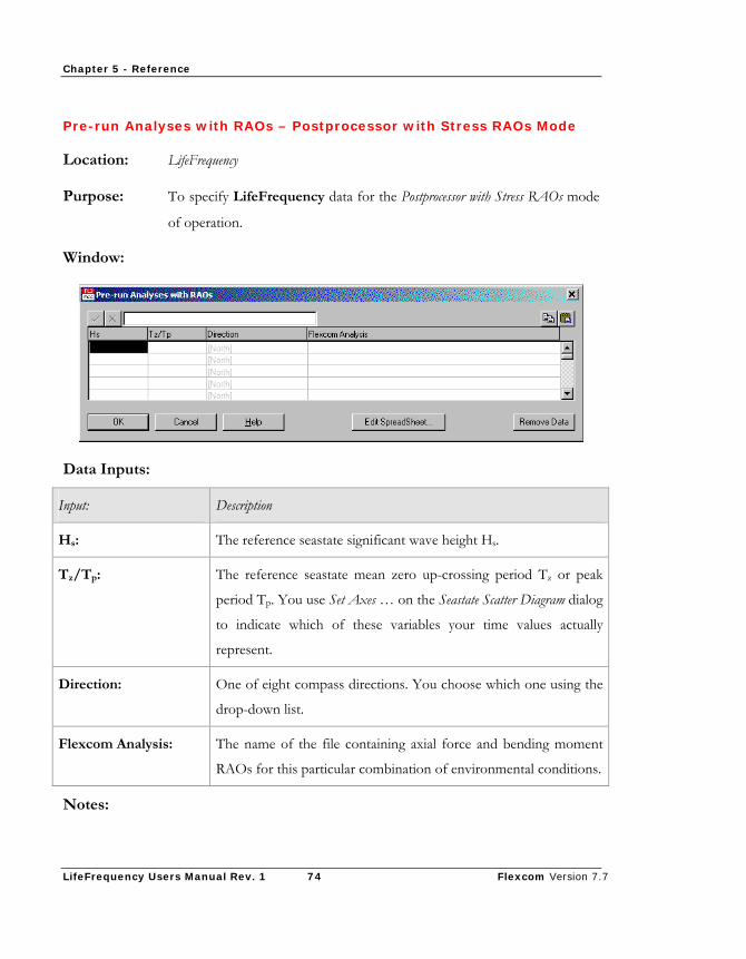
Chapter 5 - Reference
LifeFrequency Users Manual Rev. 1 74 Flexcom Version 7.7
Pre-run Analyses with RAOs – Postprocessor with Stress RAOs Mode
Location: LifeFrequency
Purpose: To specify LifeFrequency data for the Postprocessor with Stress RAOs mode
of operation.
Window:
Data Inputs:
Input: Description
Hs: The reference seastate significant wave height Hs.
Tz/Tp: The reference seastate mean zero up-crossing period Tz or peak
period Tp. You use Set Axes … on the Seastate Scatter Diagram dialog
to indicate which of these variables your time values actually
represent.
Direction: One of eight compass directions. You choose which one using the
drop-down list.
Flexcom Analysis: The name of the file containing axial force and bending moment
RAOs for this particular combination of environmental conditions.
Notes:
Chapter 5 - Reference
LifeFrequency Users Manual Rev. 1 75 Flexcom Version 7.7
(a) You must specify an RAO file name here for each reference seastate for each direction
with non-zero % occurrence.
(b) You do not need to specify a file type in the Flexcom Analysis input, just the analysis root
or generic name.

Chapter 6 - Example Drilling Riser Fatigue Analysis
LifeFrequency Users Manual Rev. 1 77 Flexcom Version 7.7
CHAPTER 6 - EXAMPLE DRILLING RISER FATIGUE
ANALYSIS
This chapter describes an example LifeFrequency fatigue analysis of a drilling riser, and is
divided into the following sections:
− ‘Introduction’ gives an overview of the example and describes the structure under
consideration.
− ‘Environment’ summarises the environmental conditions and tabulates the load cases
used.
− ‘Fatigue Data’ presents the fatigue-specific data used in the example.
− ‘Results’ summarises the results obtained.
− ‘Example Files’ lists the names of the files containing the input data for this example, all
of which are provided with the software.
INTRODUCTION
In this chapter the operation of LifeFrequency in the so-called Stand-alone mode of Chapter
2 is illustrated by means of an example fatigue analysis of a drilling riser. The riser analysed is
that used in Chapter 2, ‘Example 1 – Deepwater Drilling Riser’, of the Flexcom Examples
Manual. For a schematic of the riser stack-up and a summary of the riser input data you are
referred to Chapter 2 of the Flexcom Examples Manual.
In the LifeFrequency Category i) data specification for this example fatigue analysis, no
current or offset is specified. Imperial units are used throughout. Thickness effects are
ignored, and the fatigue analysis is based on bending stresses only.
ENVIRONMENT
The wave scatter diagram describing long-term environmental conditions for this fatigue
analysis is shown in Table 6.1. Hs values vary between 0.5 ft and 20 ft, and Tz values vary

Chapter 6 - Example Drilling Riser Fatigue Analysis
LifeFrequency Users Manual Rev. 1 78 Flexcom Version 7.7
between 4 and 13 seconds. The data in Table 6.1 is not intended to represent any particular
location, merely to demonstrate the operation of the software.
Table 6-1: Drilling Riser Fatigue Analysis – Wave Scatter Diagram
Tz (s)
4 5 6 7 8 9 10 11 12 13 0.5 136076 252100 255434 235832
2 321287 334477 298020 74558
3.5 272100 362849 383204 143217 167188
5 174127 296125 308157 275432 110168
6.5 175352 264871 260697 126533
8 117157 233065 231621 110175
Hs 9.5 111420 143196 102307 93240
(ft) 11 83161 90355 80073
12.5 67966 52943
14 32669 36253
15.5 11986 20976
17 13739
18.5 10200
20 1520 279
Three blocking schemes are used in this example to group the seastates of Table 6.1 into
blocks. The first scheme is shown in Table 6.2, which shows the scatter diagram divided into
12 blocks. A reference seastate is nominated for each block; the most frequently occurring
seastate is used. This scheme might be considered a reasonably standard application of the
blocking facility for this environmental specification.
The second blocking scheme is a variation on the first. 12 blocks are again specified, but in
this case there is only one seastate per block (which is by definition then the reference
seastate for that block). This scheme is illustrated in Table 6.3; note that the number of
occurrences per block is the same as in Table 6.2, except that in Table 6.3 all occurrences are
assigned to a single seastate. Running LifeFrequency in this way is similar to the so-called
Postprocessor with Stress Spectra mode of Chapter 3, except that LifeFrequency performs the
actual Flexcom runs in this case.

Chapter 6 - Example Drilling Riser Fatigue Analysis
LifeFrequency Users Manual Rev. 1 79 Flexcom Version 7.7
Table 6-2: Scatter Diagram Blocking Scheme – Multiple Blocks
Tz (s)
4 5 6 7 8 9 10 11 12 13 0.5 136076 252100 255434 235832
2 321287 334477 298020 74558
3.5 272100 362849 383204 143217 167188
5 174127 296125 308157 275432 110168
6.5 175352 264871 260697 126533
8 117157 233065 231621 110175
Hs 9.5 111420 143196 102307 93240
(ft) 11 83161 90355 80073
12.5 67966 52943
14 32669 36253
15.5 11986 20976
17 13739
18.5 10200
20 1520 279
Table 6-3: Scatter Diagram Blocking Scheme – Single-Sea Blocks
Tz (s)
4 5 6 7 8 9 10 11 12 13 0.5
2 709463 1198321
3.5 809076 1136043
5 552788
6.5 790445 619026
8
Hs 9.5 337777 365975
(ft) 11
12.5 189831
14
15.5 46701
17
18.5 2799
20

Chapter 6 - Example Drilling Riser Fatigue Analysis
LifeFrequency Users Manual Rev. 1 80 Flexcom Version 7.7
In the third blocking scheme one block only comprising the total scatter diagram is specified.
In this case the sole reference seastate is that with a Hs of 3.5 ft and Tz of 7 seconds (this is
the most commonly occurring seastate in the scatter diagram). The purpose of using these
three blocking schemes is obviously to compare the effect on fatigue life estimates of using
one and multiple blocks.
Likewise two directionality specifications are used in the example. These are shown in Table
6.4. In the first specification, waves approach from all eight compass directions, with %
occurrence values as shown in the table. In the second specification, waves approach from
one direction only, this being nominally the North.
Table 6-4: Directionality Specifications
Direction Case #1 Case #2
N 10% 100%
NW 15% 0%
W 5% 0%
SW 13% 0%
S 7% 0%
SE 8% 0%
E 21% 0%
NE 21% 0%
The three wave scatter diagram blocking schemes and the two directionality specifications are
combined into four overall environmental specifications or fatigue load cases as shown in
Table 6.5.

Chapter 6 - Example Drilling Riser Fatigue Analysis
LifeFrequency Users Manual Rev. 1 81 Flexcom Version 7.7
Table 6-5: Load Case Matrix
Load Case No. of Blocks No. of Seastates No. of Directions
1 1 43 1
2 12 43 1
3 12 12 1
4 12 43 8
As a check on the LifeFrequency computations, a time domain analysis with the Flexcom
fatigue postprocessor LifeTime is also undertaken for Load Case #3, corresponding to the
scatter diagram of Table 6.3 and one direction only. Results from this run are compared with
the LifeFrequency output in the ‘Results’ section later.
The dynamic analyses of this riser in the Flexcom Examples Manual consider a 2D
environment only (collinear waves, current and vessel motions). So RAOs at a single wave
heading only are included in the analysis specification. For this fatigue analysis, the simplified
RAO specification of the Examples Manual is replaced by RAOs defined as functions of
both frequency and wave direction. Specifically, the RAOs, which are typical of those for a
semi-sub, are defined at 17 wave headings and at 40 frequencies at each heading.
FATIGUE DATA
Fatigue data comprises the analysis SCF and S-N curve. For this example a stress
concentration factor of 1.5 is used throughout. The analysis S-N curve is an approximation
to the British Welding Institute Curve F, which is a log-linear curve with m and K values of
2.8 and 1.14815E9 respectively.
RESULTS
In the four fatigue analyses or Load Cases of this example, fatigue life estimates are requested
at 16 locations, these being from Elements 142 to 282 inclusive in steps of 10 elements, and
at Element 291. There is no particular significance to these locations and in reality very many
more hot spots would probably be specified. Figure 6-1 below compares the predicted

Chapter 6 - Example Drilling Riser Fatigue Analysis
LifeFrequency Users Manual Rev. 1 82 Flexcom Version 7.7
fatigue lives at these 16 locations for each of the four Load Cases. (Note the log scale on the
vertical axis.) In addition, Table 6.6 compares results at the two locations where the lowest
fatigue lives occur, near both the lower and upper flex joints.
0 1000 2000 3000 4000 5000 6000 7000 8000Distance Along Hot Spot Set (ft)
100
1000
1000
010
0000
Min
. Fat
igue
Life
(Yea
rs)
Load Case 1Load Case 2Load Case 3
Load Case 4
Figure 6-1: Comparison of LifeFrequency Results
Table 6-6: Summary of LifeFrequency Results
Minimum Fatigue Life (years) Load Case
Near Lower Flex Joint Near Telescopic Joint
1 273 261
2 695 256
3 844 343
4 2305 913
The results from Load Case 1 appear unreliable, certainly in the lower sections of the riser. It
is possible that another choice of reference seastate might produce fatigue life estimates in

Chapter 6 - Example Drilling Riser Fatigue Analysis
LifeFrequency Users Manual Rev. 1 83 Flexcom Version 7.7
better agreement with the other Load Cases – one possibility might be a seastate nearer the
‘middle’ of the scatter diagram, such as the combination of Hs = 9.5 ft and Tz = 8 seconds.
However the difficulty with this type of specification (one reference seastate only) is that in
the absence of the results from the other Load Cases it is difficult to benchmark the choice
of the one reference seastate. The results from Load Cases 2 and 3 show reasonable
agreement, with the analysis using RAOs predicting slightly higher fatigue lives.
A check on the Load Case 3 results is provided in Fig. 6.2, where the LifeFrequency results
for this case are compared with corresponding results from the Flexcom postprocessor
LifeTime. Note that the time domain results are based on only 30 minutes of simulation for
each of the 12 individual random seastates. Tables 6.7 compares the minimum fatigue lives
from the two programs in a similar format to Table 6.6. ‘Lower’ in Table 6.7 refers to the
region near the lower flex joint, while ‘Upper’ refers to the corresponding area near the
telescopic joint.
100
1000
10000
0 1000 2000 3000 4000 5000 6000 7000 8000
Fatigue Life (years)
Distance along Hot Spot Set (ft)
LifeFrequency
LifeTime: Statistics
LifeTime: Spectra
LifeTime: Rainflow
Figure 6-2: Comparison of LifeFrequency and LifeTime for Load Case 3
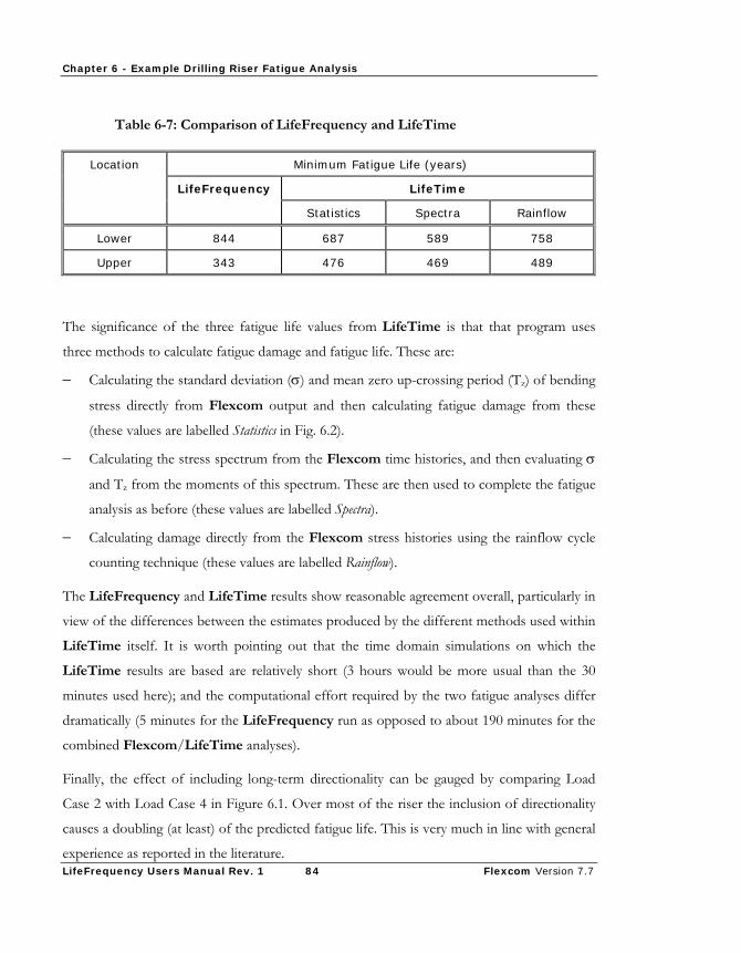
Chapter 6 - Example Drilling Riser Fatigue Analysis
LifeFrequency Users Manual Rev. 1 84 Flexcom Version 7.7
Table 6-7: Comparison of LifeFrequency and LifeTime
Minimum Fatigue Life (years)
LifeTime
Location
LifeFrequency
Statistics Spectra Rainflow
Lower 844 687 589 758
Upper 343 476 469 489
The significance of the three fatigue life values from LifeTime is that that program uses
three methods to calculate fatigue damage and fatigue life. These are:
− Calculating the standard deviation (σ) and mean zero up-crossing period (Tz) of bending
stress directly from Flexcom output and then calculating fatigue damage from these
(these values are labelled Statistics in Fig. 6.2).
− Calculating the stress spectrum from the Flexcom time histories, and then evaluating σ
and Tz from the moments of this spectrum. These are then used to complete the fatigue
analysis as before (these values are labelled Spectra).
− Calculating damage directly from the Flexcom stress histories using the rainflow cycle
counting technique (these values are labelled Rainflow).
The LifeFrequency and LifeTime results show reasonable agreement overall, particularly in
view of the differences between the estimates produced by the different methods used within
LifeTime itself. It is worth pointing out that the time domain simulations on which the
LifeTime results are based are relatively short (3 hours would be more usual than the 30
minutes used here); and the computational effort required by the two fatigue analyses differ
dramatically (5 minutes for the LifeFrequency run as opposed to about 190 minutes for the
combined Flexcom/LifeTime analyses).
Finally, the effect of including long-term directionality can be gauged by comparing Load
Case 2 with Load Case 4 in Figure 6.1. Over most of the riser the inclusion of directionality
causes a doubling (at least) of the predicted fatigue life. This is very much in line with general
experience as reported in the literature.

Chapter 6 - Example Drilling Riser Fatigue Analysis
LifeFrequency Users Manual Rev. 1 85 Flexcom Version 7.7
EXAMPLE FILES
The input files for this example may be found in the ‘Examples\LifeFrequency
Examples\Example 1 - Drilling Riser’ subdirectory of the Flexcom installation directory and
are as follows:
− Static.fl3 Flexcom file with basic riser model data.
− Semi-sub.ves Vessel RAO file.
− Load Case 1.fl3 LifeFrequency file for Load Case 1.
− Load Case 2.fl3 LifeFrequency file for Load Case 2.
− Load Case 3.fl3 LifeFrequency file for Load Case 3.
− Load Case 4.fl3 LifeFrequency file for Load Case 4.


Chapter 7 - Example SCR Fatigue Analysis with Stress Spectra
LifeFrequency Users Manual Rev. 1 87 Flexcom Version 7.7
CHAPTER 7 - EXAMPLE SCR FATIGUE ANALYSIS WITH
STRESS SPECTRA
This chapter describes an example LifeFrequency fatigue analysis of an SCR using stress
spectra, and is divided into the following sections:
− ‘Introduction’ gives an overview of the example.
− ‘Model’ describes the structure under consideration.
− ‘Environment’ summarises the environmental conditions and tabulates the fatigue load
case matrix.
− ‘Fatigue Data’ presents the fatigue-specific data used in the example.
− ‘Results’ summarises the results obtained.
− ‘Example Files’ lists the names of the files containing the input data for this example, all
of which are provided with the software.
INTRODUCTION
In this chapter the operation of LifeFrequency in the so-called Postprocessor with Stress Spectra
mode of Chapter 3 is illustrated by means of an example fatigue analysis of an SCR. The
method used to carry out the fatigue analysis involves first using Flexcom to find the initial
static configuration of the SCR. This is then followed by a series of Flexcom random sea
analyses to determine the dynamic riser response to the fatigue load case matrix.
LifeFrequency is finally run in the program Postprocessor with Stress Spectra mode of operation,
to accumulate the fatigue damage from the individual seastates.
MODEL
The SCR is 2000m in length, situated in a water depth of 820m, which is filled with export
gas at an internal pressure of 15 MPa. The SCR is fixed to the seabed at a PLEM, and is
attached to a semi-submersible platform via a flex joint with a rotational stiffness of 40
kNm/°, at a distance of 10 m below the MWL. The horizontal distance between the PLEM

Chapter 7 - Example SCR Fatigue Analysis with Stress Spectra
LifeFrequency Users Manual Rev. 1 88 Flexcom Version 7.7
and the top of the riser is 1618m. The seabed is modelled as an elastic surface with a stiffness
of 70kN/m/m. Figure 7.1 diagrammatically depicts the SCR configuration.
Length of SCR = 2000 m
Semi-Submersible
Seabed
MWL
820 m
Hang-off angle, = 22 degreesθ
θ
Figure 7.1. Schematic of SCR Configuration
A total of 242 elements are used in the model, of which 240 are SCR elements. The
maximum element length is 10m, the length of the adjoining elements are progressively
reduced in length to a minimum length of 1m situated about 30m in the touchdown zone and
in the region of the vessel connection. The structural properties and environmental data used
in this analysis are summarised in the ‘Input Data’ section below.
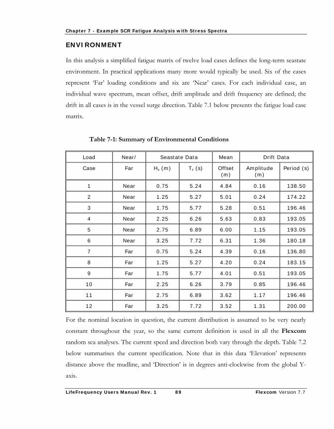
Chapter 7 - Example SCR Fatigue Analysis with Stress Spectra
LifeFrequency Users Manual Rev. 1 89 Flexcom Version 7.7
ENVIRONMENT
In this analysis a simplified fatigue matrix of twelve load cases defines the long-term seastate
environment. In practical applications many more would typically be used. Six of the cases
represent ‘Far’ loading conditions and six are ‘Near’ cases. For each individual case, an
individual wave spectrum, mean offset, drift amplitude and drift frequency are defined; the
drift in all cases is in the vessel surge direction. Table 7.1 below presents the fatigue load case
matrix.
Table 7-1: Summary of Environmental Conditions
Load Near/ Seastate Data Mean Drift Data
Case Far Hs (m) Tz (s) Offset (m)
Amplitude (m)
Period (s)
1 Near 0.75 5.24 4.84 0.16 138.50
2 Near 1.25 5.27 5.01 0.24 174.22
3 Near 1.75 5.77 5.28 0.51 196.46
4 Near 2.25 6.26 5.63 0.83 193.05
5 Near 2.75 6.89 6.00 1.15 193.05
6 Near 3.25 7.72 6.31 1.36 180.18
7 Far 0.75 5.24 4.39 0.16 136.80
8 Far 1.25 5.27 4.20 0.24 183.15
9 Far 1.75 5.77 4.01 0.51 193.05
10 Far 2.25 6.26 3.79 0.85 196.46
11 Far 2.75 6.89 3.62 1.17 196.46
12 Far 3.25 7.72 3.52 1.31 200.00
For the nominal location in question, the current distribution is assumed to be very nearly
constant throughout the year, so the same current definition is used in all the Flexcom
random sea analyses. The current speed and direction both vary through the depth. Table 7.2
below summarises the current specification. Note that in this data ‘Elevation’ represents
distance above the mudline, and ‘Direction’ is in degrees anti-clockwise from the global Y-
axis.
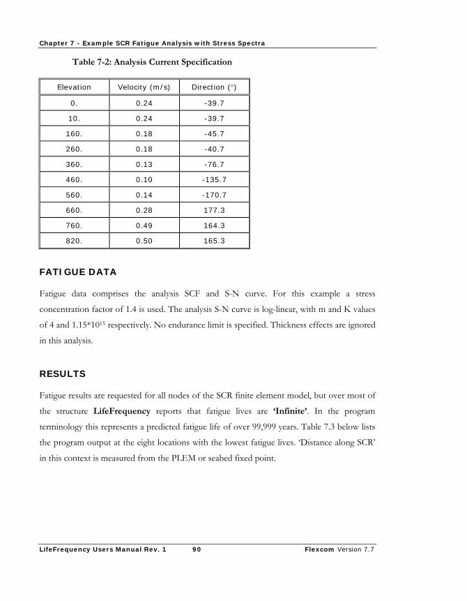
Chapter 7 - Example SCR Fatigue Analysis with Stress Spectra
LifeFrequency Users Manual Rev. 1 90 Flexcom Version 7.7
Table 7-2: Analysis Current Specification
Elevation Velocity (m/s) Direction (°)
0. 0.24 -39.7
10. 0.24 -39.7
160. 0.18 -45.7
260. 0.18 -40.7
360. 0.13 -76.7
460. 0.10 -135.7
560. 0.14 -170.7
660. 0.28 177.3
760. 0.49 164.3
820. 0.50 165.3
FATIGUE DATA
Fatigue data comprises the analysis SCF and S-N curve. For this example a stress
concentration factor of 1.4 is used. The analysis S-N curve is log-linear, with m and K values
of 4 and 1.15*1015 respectively. No endurance limit is specified. Thickness effects are ignored
in this analysis.
RESULTS
Fatigue results are requested for all nodes of the SCR finite element model, but over most of
the structure LifeFrequency reports that fatigue lives are ‘Infinite’. In the program
terminology this represents a predicted fatigue life of over 99,999 years. Table 7.3 below lists
the program output at the eight locations with the lowest fatigue lives. ‘Distance along SCR’
in this context is measured from the PLEM or seabed fixed point.
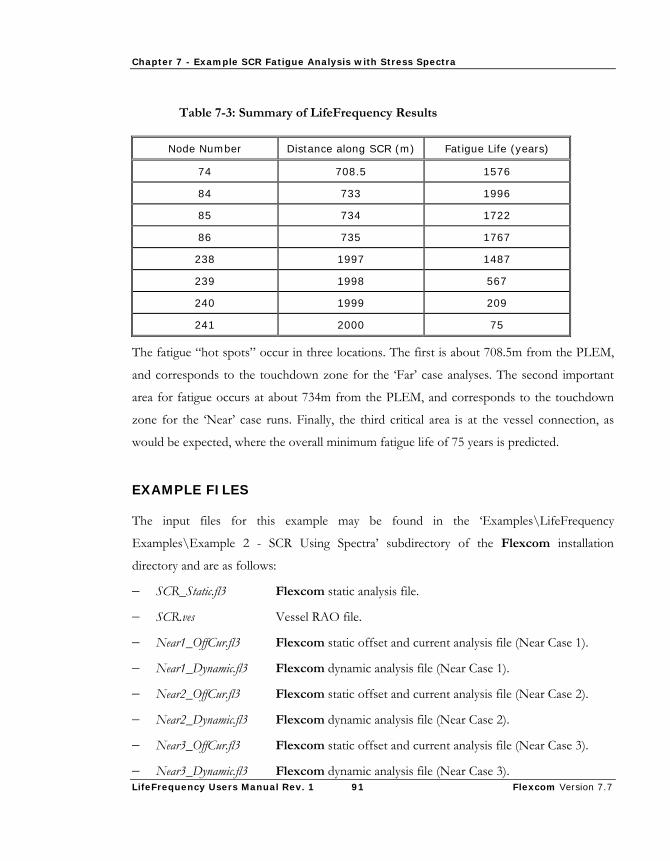
Chapter 7 - Example SCR Fatigue Analysis with Stress Spectra
LifeFrequency Users Manual Rev. 1 91 Flexcom Version 7.7
Table 7-3: Summary of LifeFrequency Results
Node Number Distance along SCR (m) Fatigue Life (years)
74 708.5 1576
84 733 1996
85 734 1722
86 735 1767
238 1997 1487
239 1998 567
240 1999 209
241 2000 75
The fatigue “hot spots” occur in three locations. The first is about 708.5m from the PLEM,
and corresponds to the touchdown zone for the ‘Far’ case analyses. The second important
area for fatigue occurs at about 734m from the PLEM, and corresponds to the touchdown
zone for the ‘Near’ case runs. Finally, the third critical area is at the vessel connection, as
would be expected, where the overall minimum fatigue life of 75 years is predicted.
EXAMPLE FILES
The input files for this example may be found in the ‘Examples\LifeFrequency
Examples\Example 2 - SCR Using Spectra’ subdirectory of the Flexcom installation
directory and are as follows:
− SCR_Static.fl3 Flexcom static analysis file.
− SCR.ves Vessel RAO file.
− Near1_OffCur.fl3 Flexcom static offset and current analysis file (Near Case 1).
− Near1_Dynamic.fl3 Flexcom dynamic analysis file (Near Case 1).
− Near2_OffCur.fl3 Flexcom static offset and current analysis file (Near Case 2).
− Near2_Dynamic.fl3 Flexcom dynamic analysis file (Near Case 2).
− Near3_OffCur.fl3 Flexcom static offset and current analysis file (Near Case 3).
− Near3_Dynamic.fl3 Flexcom dynamic analysis file (Near Case 3).

Chapter 7 - Example SCR Fatigue Analysis with Stress Spectra
LifeFrequency Users Manual Rev. 1 92 Flexcom Version 7.7
− Near4_OffCur.fl3 Flexcom static offset and current analysis file (Near Case 4).
− Near4_Dynamic.fl3 Flexcom dynamic analysis file (Near Case 4).
− Near5_OffCur.fl3 Flexcom static offset and current analysis file (Near Case 5).
− Near5_Dynamic.fl3 Flexcom dynamic analysis file (Near Case 5).
− Near6_OffCur.fl3 Flexcom static offset and current analysis file (Near Case 6).
− Near6_Dynamic.fl3 Flexcom dynamic analysis file (Near Case 6).
− Far1_OffCur.fl3 Flexcom static offset and current analysis file (Far Case 1).
− Far1_Dynamic.fl3 Flexcom dynamic analysis file (Far Case 1).
− Far2_OffCur.fl3 Flexcom static offset and current analysis file (Far Case 2).
− Far2_Dynamic.fl3 Flexcom dynamic analysis file (Far Case 2).
− Far3_OffCur.fl3 Flexcom static offset and current analysis file (Far Case 3).
− Far3_Dynamic.fl3 Flexcom dynamic analysis file (Far Case 3).
− Far4_OffCur.fl3 Flexcom static offset and current analysis file (Far Case 4).
− Far4_Dynamic.fl3 Flexcom dynamic analysis file (Far Case 4).
− Far5_OffCur.fl3 Flexcom static offset and current analysis file (Far Case 5).
− Far5_Dynamic.fl3 Flexcom dynamic analysis file (Far Case 5).
− Far6_OffCur.fl3 Flexcom static offset and current analysis file (Far Case 6).
− Far6_Dynamic.fl3 Flexcom dynamic analysis file (Far Case 6).
− SCR.fl3 LifeFrequency fatigue analysis file.
INPUT DATA
Riser Properties
Table 7.4 below summarises the structural properties used in the model.
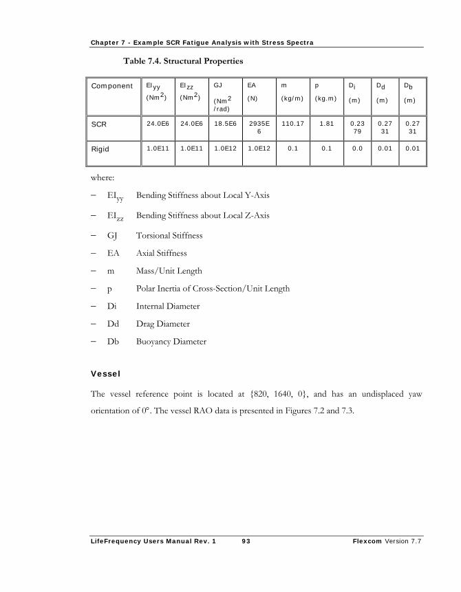
Chapter 7 - Example SCR Fatigue Analysis with Stress Spectra
LifeFrequency Users Manual Rev. 1 93 Flexcom Version 7.7
Table 7.4. Structural Properties
Component EIyy
(Nm2)
EIzz
(Nm2)
GJ
(Nm2
/rad)
EA
(N)
m
(kg/m)
p
(kg.m)
Di
(m)
Dd
(m)
Db
(m)
SCR 24.0E6 24.0E6 18.5E6 2935E6
110.17 1.81 0.2379
0.2731
0.2731
Rigid 1.0E11 1.0E11 1.0E12 1.0E12 0.1 0.1 0.0 0.01 0.01
where:
− EIyy Bending Stiffness about Local Y-Axis
− EIzz Bending Stiffness about Local Z-Axis
− GJ Torsional Stiffness
− EA Axial Stiffness
− m Mass/Unit Length
− p Polar Inertia of Cross-Section/Unit Length
− Di Internal Diameter
− Dd Drag Diameter
− Db Buoyancy Diameter
Vessel
The vessel reference point is located at {820, 1640, 0}, and has an undisplaced yaw
orientation of 0°. The vessel RAO data is presented in Figures 7.2 and 7.3.

Chapter 7 - Example SCR Fatigue Analysis with Stress Spectra
LifeFrequency Users Manual Rev. 1 94 Flexcom Version 7.7
0
0.2
0.4
0.6
0.8
1
1.2
1.4
1.6
0 0.05 0.1 0.15 0.2 0.25 0.3 0.35 0.4 0.45 0.5
Frequency (Hz)
RA
O (m
/m o
r deg
/m)
Heave Surge Pitch
Figure 7.2. Heave, Surge and Pitch RAOs
0
50
100
150
200
250
300
350
400
0 0.05 0.1 0.15 0.2 0.25 0.3 0.35 0.4 0.45 0.5
Frequency (Hz)
Phas
e A
ngle
(deg
)
Heave Surge Pitch
Figure 7.3. Heave, Surge and Pitch Phase Angles

Chapter 7 - Example SCR Fatigue Analysis with Stress Spectra
LifeFrequency Users Manual Rev. 1 95 Flexcom Version 7.7
Internal Fluid
The riser is gas filled a
s follows:
Table 7.5. Internal Fluid Properties
Height (m) Density (kg/m3) Pressure (MPa)
290.0 880.0 18.008
−


Chapter 8 - Example SCR Fatigue Analysis with RAOs
LifeFrequency Users Manual Rev. 1 97 Flexcom Version 7.7
CHAPTER 8 - EXAMPLE SCR FATIGUE ANALYSIS WITH
RAOS
This chapter describes an example LifeFrequency fatigue analysis of an SCR using stress
RAOs, and is divided into the following sections:
− ‘Introduction’ gives an overview of the example and describes the structure under
consideration.
− ‘Environment’ summarises the environmental conditions and tabulates the fatigue load
case matrix.
− ‘Fatigue Data’ presents the fatigue-specific data used in the example.
− ‘Results’ summarises the results obtained.
− ‘Example Files’ lists the names of the files containing the input data for this example, all
of which are provided with the software.
INTRODUCTION
In this chapter the operation of LifeFrequency in the so-called Postprocessor with RAOs mode
of Chapter 4 is illustrated by means of an example fatigue analysis of an SCR. The riser
analysed is the same as that used in the example in the previous chapter. Specifically, an SCR
of length 2000m in 820m of water is considered. The seabed is modelled as an elastic surface
with a stiffness of 70kN/m/m. For a schematic of the SCR configuration and a summary of
the riser input data you are referred to the previous chapter.
The method used to carry out the fatigue analysis involves first using Flexcom to find the
initial static configuration of the SCR. This is followed by a series of Flexcom random sea
analyses to determine the dynamic riser response to specified reference seastates. These
analyses are then postprocessed using Flexcom to generate stress RAOs for specified points
along the riser. LifeFrequency is finally run in the program Postprocessor with RAOs mode of
operation, to accumulate the fatigue damage from the scatter diagram seastates.

Chapter 8 - Example SCR Fatigue Analysis with RAOs
LifeFrequency Users Manual Rev. 1 98 Flexcom Version 7.7
ENVIRONMENT
The wave scatter diagram describing long-term environmental conditions for this fatigue
analysis is shown in Table 8.1. Hs values vary between 0.3 m and 4.2 m, and Tz values vary
between 1 and 10 seconds. The data in Table 8.1 is effectively the scatter diagram from the
drilling riser analysis of Chapter 6 converted to Metric, and is not intended to represent any
particular location.
Table 8-1: Scatter Diagram Blocking Scheme
Tz (s)
1 2 3 4 5 6 7 8 9 10 0.3 136076 252100 255434 235832 0.6 270372 354477 298020 74558
0.9 272100 562849 323204 148217 167188 1.2 174127 296125 308157 275432 110168
1.5 175352 244871 240697 126533 1.8 117157 233065 231621 110175
Hs 2.1 111420 143196 96346 93240
(m) 2.4 83161 90355 65073
2.7 55672 32943 3.0 32669 26253
3.3 8101 15346 3.6 10232
3.9 10200 4.2 1520 279
The scatter diagram is divided into 12 blocks. A reference seastate is nominated for each
block; the most frequently occurring seastate is used. For this example the directionality data
has a non-zero occurrence for one direction only, nominally North.
For each reference seastate, the current distribution is assumed to be very nearly constant
throughout the year, so the same current definition is used in all the Flexcom random sea
analyses. The current speed varies through the depth. Table 8.2 below summarises the
current specification. Note that in this data ‘Elevation’ represents distance above the
mudline, and ‘Direction’ is in degrees anti-clockwise from the global Y-axis.

Chapter 8 - Example SCR Fatigue Analysis with RAOs
LifeFrequency Users Manual Rev. 1 99 Flexcom Version 7.7
Table 8-2: Analysis Current Specification
Elevation Velocity (m/s) Direction (º)
0. 0.24 10.0
10. 0.24 10.0
160. 0.18 10.0
260. 0.18 10.0
360. 0.13 10.0
460. 0.10 10.0
560. 0.14 10.0
660. 0.28 10.0
760. 0.49 10.0
820. 0.50 10.0
FATIGUE DATA
Fatigue data comprises the analysis SCF and S-N curve. For this example a stress
concentration factor of 1.2 is used. The analysis S-N curve is log-linear, with m and K values
of 3 and 4.27*1011 respectively. No endurance limit is specified. Thickness effects are ignored
in this analysis.
RESULTS
Fatigue results are requested for 25 locations along the SCR finite element model, these being
from Elements 1 to 231 inclusive in steps of 10 elements, and Element 240. There is no
particular significance to these locations and in a real-world analysis very many more hot
spots would probably be specified. Table 8.3 below lists the program output at the four
locations with the lowest fatigue lives. ‘Distance along SCR’ in this context is measured from
the PLEM or seabed fixed point.
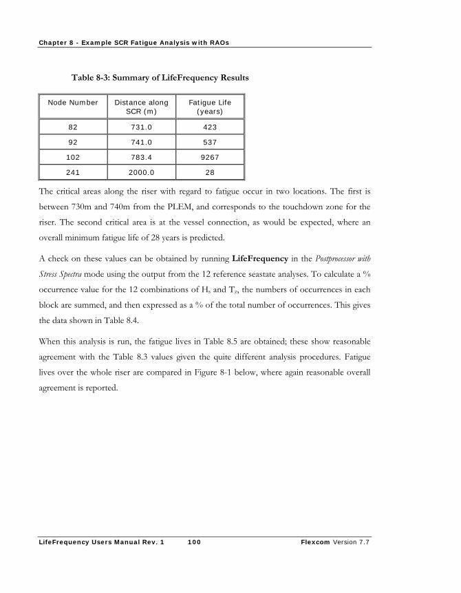
Chapter 8 - Example SCR Fatigue Analysis with RAOs
LifeFrequency Users Manual Rev. 1 100 Flexcom Version 7.7
Table 8-3: Summary of LifeFrequency Results
Node Number Distance along SCR (m)
Fatigue Life (years)
82 731.0 423
92 741.0 537
102 783.4 9267
241 2000.0 28
The critical areas along the riser with regard to fatigue occur in two locations. The first is
between 730m and 740m from the PLEM, and corresponds to the touchdown zone for the
riser. The second critical area is at the vessel connection, as would be expected, where an
overall minimum fatigue life of 28 years is predicted.
A check on these values can be obtained by running LifeFrequency in the Postprocessor with
Stress Spectra mode using the output from the 12 reference seastate analyses. To calculate a %
occurrence value for the 12 combinations of Hs and Tz, the numbers of occurrences in each
block are summed, and then expressed as a % of the total number of occurrences. This gives
the data shown in Table 8.4.
When this analysis is run, the fatigue lives in Table 8.5 are obtained; these show reasonable
agreement with the Table 8.3 values given the quite different analysis procedures. Fatigue
lives over the whole riser are compared in Figure 8-1 below, where again reasonable overall
agreement is reported.

Chapter 8 - Example SCR Fatigue Analysis with RAOs
LifeFrequency Users Manual Rev. 1 101 Flexcom Version 7.7
Table 8-4: Seastate % Occurrences for Check Analysis
Hs Tz % Occurrence
3.9 9 0.2
3.3 9 0.5
2.7 7 2.2
2.1 7 5
2.1 6 4.9
1.5 6 10.3
1.5 5 11.2
1.2 6 8
0.9 4 15.7
0.9 3 14.7
0.6 3 17.7
0.6 2 9.6
Table 8-5: LifeFrequency Results, Postprocessor with Stress Spectra Mode
Node Number Distance along SCR (m) Fatigue Life (years)
82 731.0 535
92 741.0 677
102 783.4 11510
241 2000.0 36
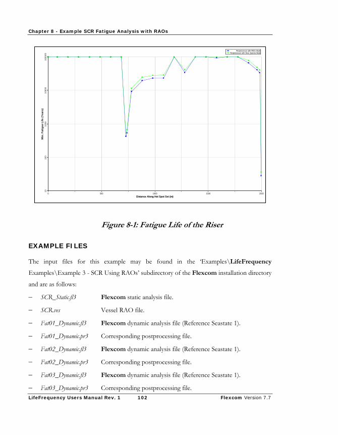
Chapter 8 - Example SCR Fatigue Analysis with RAOs
LifeFrequency Users Manual Rev. 1 102 Flexcom Version 7.7
0 500 1000 1500 2000Distance Along Hot Spot Set (m)
1010
010
0010
000
1000
00M
in. F
atig
ue L
ife (Y
ears
)
Postprocessor with RAOs ModePostprocessor with Stres Spectra Mode
Figure 8-1: Fatigue Life of the Riser
EXAMPLE FILES
The input files for this example may be found in the ‘Examples\LifeFrequency
Examples\Example 3 - SCR Using RAOs’ subdirectory of the Flexcom installation directory
and are as follows:
− SCR_Static.fl3 Flexcom static analysis file.
− SCR.ves Vessel RAO file.
− Fat01_Dynamic.fl3 Flexcom dynamic analysis file (Reference Seastate 1).
− Fat01_Dynamic.pr3 Corresponding postprocessing file.
− Fat02_Dynamic.fl3 Flexcom dynamic analysis file (Reference Seastate 1).
− Fat02_Dynamic.pr3 Corresponding postprocessing file.
− Fat03_Dynamic.fl3 Flexcom dynamic analysis file (Reference Seastate 1).
− Fat03_Dynamic.pr3 Corresponding postprocessing file.

Chapter 8 - Example SCR Fatigue Analysis with RAOs
LifeFrequency Users Manual Rev. 1 103 Flexcom Version 7.7
− Fat04_Dynamic.fl3 Flexcom dynamic analysis file (Reference Seastate 1).
− Fat04_Dynamic.pr3 Corresponding postprocessing file.
− Fat05_Dynamic.fl3 Flexcom dynamic analysis file (Reference Seastate 1).
− Fat05_Dynamic.pr3 Corresponding postprocessing file.
− Fat06_Dynamic.fl3 Flexcom dynamic analysis file (Reference Seastate 1).
− Fat06_Dynamic.pr3 Corresponding postprocessing file.
− Fat07_Dynamic.fl3 Flexcom dynamic analysis file (Reference Seastate 1).
− Fat07_Dynamic.pr3 Corresponding postprocessing file.
− Fat08_Dynamic.fl3 Flexcom dynamic analysis file (Reference Seastate 1).
− Fat08_Dynamic.pr3 Corresponding postprocessing file.
− Fat09_Dynamic.fl3 Flexcom dynamic analysis file (Reference Seastate 1).
− Fat09_Dynamic.pr3 Corresponding postprocessing file.
− Fat10_Dynamic.fl3 Flexcom dynamic analysis file (Reference Seastate 1).
− Fat10_Dynamic.pr3 Corresponding postprocessing file.
− Fat11_Dynamic.fl3 Flexcom dynamic analysis file (Reference Seastate 1).
− Fat11_Dynamic.pr3 Corresponding postprocessing file.
− Fat12_Dynamic.fl3 Flexcom dynamic analysis file (Reference Seastate 1).
− Fat12_Dynamic.pr3 Corresponding postprocessing file.
− SCR.fl3 LifeFrequency fatigue analysis file