Life Span: Evolutionary, Ecological, and Demographic ...€¦ · uses an explicitly evolutionary...
308
A Supplement to Vol. 29, 2003 James R. Carey Shripad Tuljapurkar Editors Life Span Evolutionary, Ecological, and Demographic Perspectives
Transcript of Life Span: Evolutionary, Ecological, and Demographic ...€¦ · uses an explicitly evolutionary...

A Supplement to Vol. 29, 2003
POPULATIONANDDEVELOPMENTREVIEW
Life
Sp
an
Carey
/T
ulja
pu
rk
ar
Pop
ula
tio
n C
ou
ncil
James R. Carey
Shripad Tuljapurkar
Editors
Life Span
Evolutionary, Ecological,and DemographicPerspectives
The human life span continues to increase even in already low-mortality
populations—with major implications for societies and economies.
Classical evolutionary theory accounts for survival only through the
age of reproduction. A more elaborate theory, integrating biological
and demographic perspectives, is required to explain these current
trends in longevity and to gauge their future course. The papers col-
lected in this volume contribute to the development of such a theo-
ry. The authors are leading scientists from demography, evolutionary
biology, and field ecology, equipped to draw insights not only from
human populations but also from the comparative mortality pat-
terns and environmental circumstances of many other species: mam-
mals, birds, fish, and insects. The opening chapter presents an
overview of the evolutionary and genetic bases of aging and senes-
cence, within and between species, and of the additional role of social
evolution. Subsequent chapters explore the selective forces that shape
life span patterns in various species—not least, in fruit flies; present
an economic optimization model of the evolution of life span; and
analyze the surprising phenomenon of the apparent slowing of the
rate of increase in human mortality with age at the oldest ages. A
final chapter attempts a synthesis of the various approaches to
explaining and predicting age patterns of mortality.
About the Editors James R. Carey is Professor, Department of Entomology,University of California at Davis; and Senior Scholar, Center for the Economicsand Demography of Aging, University of California at Berkeley. ShripadTuljapurkar is Morrison Professor of Population Studies and Professor ofBiological Sciences, Stanford University.
Cover design by Charles & Ruth Kaplan

Population and Development Review seeks toadvance knowledge of the interrelationships betweenpopulation and socioeconomic development andprovides a forum for discussion of related issues of public policy.
EDITOR Paul Demeny
MANAGING EDITOR Ethel P. Churchill
EDITORIAL COMMITTEE
Paul Demeny, Chair Geoffrey McNicollEthel P. Churchill Michael P. TodaroSusan Greenhalgh
EDITORIAL STAFF
Robert Heidel, Production EditorY. Christina Tse, Production/DesignMargaret A. Knoll, CirculationSura Rosenthal / Mike Vosika, Production
ADVISORY BOARD
John C. Caldwell Milos̆ MacuraMercedes B. Concepción Carmen A. MiróRichard A. Easterlin Asok MitraAkin L. Mabogunje Samuel H. Preston
Signed articles are the responsibility of the authors.Views expressed in the Review do not necessarily reflectthe views of the Population Council.
Direct manuscripts, comments on articles, and correspondence to:
Population and Development ReviewPopulation CouncilOne Dag Hammarskjold PlazaNew York, New York 10017 USA
Electronic submissions are encouraged and should be sent [email protected]
Support from the United Nations Population Fund is gratefullyacknowledged.
The website for Population and Development Review iswww.popcouncil.org/pdr. Subscribers have access to the electronic editionof the journal, which is published simultaneously with the printed issue.
The full contents of Volumes 1–26 (1975–2000) are available throughparticipating libraries from JSTOR at www.jstor.org/journals/00987921.html
INFORMATION FOR SUBSCRIBERS
Population and Development Review is available on a paidsubscription basis at the following rates:
One year (4 issues) US$40.00 Two years (8 issues) US$64.00
To enter a subscription, send payment by check or money order drawn on aUS bank, payable to the Population Council, or by American Express,MasterCard, or Visa (provide card number and expiration date), togetherwith mailing address to the address given above.
Credit card orders may also be placed by phone to (212) 339-0514, by faxto (212) 755-6052, or by e-mail to [email protected]
Complimentary subscriptions are available to qualified applicants residingin developing countries. Individuals and institutions wishing to apply forcomplimentary subscriptions should send requests on letterhead stationeryto the above address stating the nature of professional involvement indevelopment- and population-related issues.
Volumes are available on microfilm from Xerox University Microfilms,300 North Zeeb Road, Ann Arbor, Michigan 48106.
PDR 29 Supp inside front cover 7/6/06, 3:11 PM1

LIFE SPAN:EVOLUTIONARY, ECOLOGICAL,AND DEMOGRAPHICPERSPECTIVES


LIFE SPAN:EVOLUTIONARY,ECOLOGICAL,AND DEMOGRAPHICPERSPECTIVESJames R. CareyShripad TuljapurkarEditors
POPULATION AND DEVELOPMENT REVIEWA Supplement to Volume 29, 2003
POPULATION COUNCILNew York

Printed in the United States of America.
©2003 by The Population Council, Inc. All rights reserved.
Library of Congress Cataloging-in-Publication Data
Life span : evolutionary, ecological, and demographic perspectives / James R. Carey,Shripad Tuljapurkar, editors.
p. cm.
Includes bibliographical references.
ISBN 0-87834-111-0 (pbk. : alk. paper)
1. Life spans (Biology) 2. Longevity. 3. Population biology. 4. Demography. I. Carey,James R. II. Tuljapurkar, Shripad, 1951-
QP85 .L583 2003
612.6’8—dc21 2003042903
ISSN 0098-7921ISBN 0-87834-111-0

CONTENTS
Preface vii
Acknowledgments xi
Life Span: A Conceptual Overview 1
JAMES R. CAREY
How and Why Do Aging and Life Span Evolve? 19
STEVEN HECHT ORZACK
Ecological Correlates of Life Span in Populations 39of Large Herbivorous Mammals
JEAN-MICHEL GAILLARD
ANNE LOISON
MARCO FESTA-BIANCHET
NIGEL GILLES YOCCOZ
ERLING SOLBERG
Environment and Longevity: The Demography of theGrowth Rate 57
MARC MANGEL
Life Span in the Light of Avian Life Histories 71
ROBERT E. RICKLEFS
ALEX SCHEUERLEIN
Life Span Extension of Drosophila melanogaster:Genetic and Population Studies 99
LAWRENCE G. HARSHMAN
Interspecies Differences in the Life Span Distribution:Humans versus Invertebrates 127
SHIRO HORIUCHI

Embodied Capital and the Evolutionary Economicsof the Human Life Span 152
HILLARD KAPLAN
JANE LANCASTER
ARTHUR ROBSON
Rescaling the Life Cycle: Longevity and Proportionality 183
RONALD LEE
JOSHUA R. GOLDSTEIN
Survival Beyond Age 100: The Case of Japan 208
JEAN-MARIE ROBINE
YASUHIKO SAITO
Life Course, Environmental Change, and Life Span 229
JEAN-MARIE ROBINE
The World Trend in Maximum Life Span 239
JOHN R. WILMOTH
JEAN-MARIE ROBINE
Post-Darwinian Longevity 258
JAMES W. VAUPEL
Hazard Curves and Life Span Prospects 270
KENNETH W. WACHTER
AUTHORS 292

PREFACE
This volume is based on a series of papers presented at the workshop “Life span:Evolutionary, ecological, and demographic perspectives,” held 14–18 May 2001at the Petros M. Nomikos Conference Centre on the Greek island of Santorini.The specific aims of the Santorini workshop were threefold: first, to bring to-gether leading scientists from demography, evolutionary biology, and field ecol-ogy to integrate and synthesize concepts in gerontology, demography, ecology,and evolution as they pertain to aging and longevity at the level of the organ-ism; second, to foster greater interaction between biologists and demographers,including the development of collaborative research on the biodemography ofaging and longevity; third, to assemble a set of papers written to be accessibleto a wide audience and designed to have lasting value to readers. To this endthe chapters in this volume have been substantially developed beyond the con-ference presentations and rigorously reviewed.
The volume is concerned with the biodemography of life span, a subjectthat has recently emerged at the confluence of demography and biology. Overthe twentieth century, human life span measured as period life expectancy hasincreased by more than 50 percent in most industrialized countries, drivingconcern about the benefits and costs of longer life and raising keen interest inwhether we can maintain the past rate of increase in life span. Biodemographybrings together methods, materials, theories, and analyses from both biologyand demography with the aim of understanding the past and anticipating thefuture of life span.
Traditionally, demographers have focused on the age pattern of deathwithin populations and on the consequences of mortality change for popula-tions, societies, and economies. Biologists have studied aging in terms of itsultimate (i.e., evolutionary) and proximate (i.e., mechanistic and genetic) causeswithin species and in terms of variability within and between populations andspecies. To set the stage, the first chapter, by James Carey, presents a broadoverview of these viewpoints and their contribution to understanding the na-ture and determinants of life span. Carey also discusses the role of social evolu-tion as a potential accelerator of increase in life span.
The thirteen chapters that follow fall in four broad groups: those con-cerned primarily with biological mechanisms, observations, or theories of ag-ing; those that develop new theories of aging that are not biologically based butuse economic or statistical arguments; those that analyze old-age mortalityamong humans; and, finally, a synthesis.
The first group begins with a theoretical overview by Steven Orzack. Heuses an explicitly evolutionary approach, based on allele frequencies and de-mographic theory, to examine the significance of environmental variability asa selective force that can shape life span in a number of significant ways. Jean-
v i i

Michel Gaillard and his coauthors present and analyze data on the age patternof mortality in several species of large herbivorous mammals, providing evi-dence of senescence in populations in the wild and of sex differences in mor-tality patterns and life span. Marc Mangel describes progress toward a moreproximate theory of mortality, showing how oxidative damage and repair canbe used in an optimization model to predict mortality patterns in fish and po-tentially in other species.
These chapters challenge the classical evolutionary theory of senescence:that natural selection must decline with age and cease after the age of last re-production. However, some empirical support for the classical theory is pro-vided here by Robert Ricklefs and Alex Scheuerlein, who present data on phy-logenetic variation in mortality and life span among wild and captive birds andmammals. Even so, they point out that the classical arguments need to be sharp-ened in terms of specific general or particular mechanisms if we are to properlyunderstand and predict age patterns of mortality.
A different, mechanistic, dimension of biological work on aging is foundin Lawrence Harshman’s review of our rapidly expanding knowledge of thegenetic determinants of life span in the fruit fly Drosophila melanogaster. In thefinal chapter of this first group, Shiro Horiuchi uses the general notion of dif-ferential selection to formulate demographic models that allow him to estimatebiologically derived heterogeneity in mortality. He estimates and compares suchvariability in populations of humans and five other species.
The evolution of human life spans may require that we move away fromstrictly biological methods and paradigms to new theories about the determi-nants of aging and of adaptation in response to aging. Hillard Kaplan and hiscoauthors take a large step away from the classical view of biological evolution,building an economically based optimization model for the evolution of lifespan. In a related vein, Ronald Lee and Joshua Goldstein consider how thehuman life cycle may adapt to increases in life span. They use scaling ideas,similar to those employed in biology, to study the temporal extension of differ-ent parts of the life cycle in the perspective of life cycle consumption.
The third group of chapters considers an important question in biodemo-graphy: the age pattern of mortality among the oldest humans. This questionbecame prominent when experiments on medflies revealed a fundamentallynew pattern of mortality change: a slowdown in the rate of mortality increasewith age. In search of the expected human parallel, Jean-Marie Robine andYasuhiko Saito, and John Wilmoth and Robine, report here on the nature andimplications of accurate data on human mortality at old ages, especially amongcentenarians. Their data add substantial support for the existence of a similarslowdown of mortality increase in humans. In a separate chapter, Robine ex-plores the idea that late-age human mortality is shaped by plasticity, the re-sponse of similar genotypes to environmental differences, rather than by selec-tion. A rather different explanation is offered by James Vaupel, who viewspostreproductive life as an epiphenomenon: natural selection cannot directlyinfluence late-age mortality, which must therefore be shaped by a different forcethat he takes to be the pattern of reliability of a complex system.
v i i i P R E F A C E

The complexity of the phenomena and theories presented here points toa major task for biodemography: the integration of detailed work on proximatemechanisms with a broader general picture applicable across species. A start ona synthesis is made here by Kenneth Wachter. He focuses on the age pattern ofmortality as a key variable, and shows how the various approaches describedhere contribute to our ability to explain and predict this age pattern. He arguesthat biodemographic understanding of mortality should inform us about thelikely challenges of achieving continued progress in extending human life spans.
Shripad Tuljapurkar
James R. Carey
P R E F A C E ix


ACKNOWLEDGMENTS
We express our appreciation to staff at the Petros M. Nomikos Conference Centrefor allowing us to use their beautiful facilities, for their efficiency throughoutthe workshop, and mostly for their warm hospitality.
We gratefully acknowledge financial support for the conference from theCenter for the Economics and Demography of Aging at the University of Cali-fornia at Berkeley and the National Institute on Aging.
This publication was supported by major contributions from the Centerfor the Economics and Demography of Aging at the University of California atBerkeley, the College of Agricultural and Environmental Sciences at the Uni-versity of California at Davis, and the Program on Population, Policy and Agingat the Terry Sanford Institute of Public Policy at Duke University, with addi-tional funding provided by Stanford University. In particular we acknowledgesupport for the publication from National Institute on Aging grant P30-AG12839awarded to Berkeley’s Center for the Economics and Demography of Agingand from National Institute on Aging grant AG08761 awarded to Duke Univer-sity; James W. Vaupel is the director of the program of research supported bythe latter grant.
We thank Monique Verrier for technical assistance. We thank the edito-rial staff of Population and Development Review for their assistance in producingthis volume.
J.R.C.
S.T.
x i


1
Life Span:A Conceptual Overview
JAMES R. CAREY
Life span is an evolved life-history characteristic of an organism that refersto the duration of its life course. Application of the concept is straightfor-ward at both individual and cohort levels: it specifies the period betweenbirth and death for the individual and the average length of life or life ex-pectancy at birth for cohorts (including both real and synthetic cohorts).When life span is applied to a population or a species, however, it requiresa modifier to avoid ambiguity (Goldwasser 2001). Maximum observed lifespan is the highest verified age at death, possibly limited to a particular popu-lation, cohort, or species in a specified time period. The overall highest veri-fied age for a species is called its record life span. The theoretical highestattainable age is known as maximum potential life span.
Maximum observed life spans (i.e., longevity records) are not synony-mous with theoretical maximums for at least two reasons. First, maximumlongevity is an inappropriate general concept because an animal dies beforethe age of infinity. It does so not because it cannot pass some boundary agebut because the probability of its avoiding the ever-present risk of death forthat long is infinitesimally small (Gavrilov and Gavrilova 1991). In other words,there is no specific identifiable age for each species to which some select indi-viduals can survive but beyond which none can live. Second, the record ageof a species is heavily influenced by the number of individuals observed. Thatis, the longevity records for a species in which the life spans of large numbersof individuals have been observed will be significantly greater than the corre-sponding figure for a species with the same longevity but represented by afew dozen individuals. For the vast majority of longevity records by species,the number of individuals at risk is unknown.
Abstract perspectives on life span
Life span should be considered within a larger biological framework con-cerned with life duration—a model where the end points of life for an indi-vidual do not necessarily correspond to the conventional events of birth
PDR 29 Supp Carey.sp 7/6/06, 3:16 PM1

2 L I F E S P A N : A C O N C E P T U A L O V E R V I E W
and death. The concept of life span does not apply to bacteria that repro-duce by binary fission, to plant species that reproduce by cloning, or to modu-lar organisms with iterated growth such as coral or honeybee colonies. Thestate of existence for an individual refers to one of several possible states ofliving such as “normal state,” metabolic reduction (e.g., hibernation), orarrest (e.g., frozen embryo; dormancy); its time of existence refers to thesum total of all stages of the individual’s life up to its extinction. What con-stitutes an individual is conditional on the level of individualism. For ex-ample, the individual cell within a multicellular organism and the individualworker bee in a colony of honeybees are individuals on one level but arepart of a greater whole on another. Death of a component part (e.g., throughapoptosis) may or may not determine the death of the whole, although ineach case the components (cells; worker bees) relinquish both their evolu-tionary heritage and their autonomy in favor of the higher organisms (or inthe case of honey bees, the colony as “super-organism”) of which they area part (Michod 1999).
The distinction between mortal macroorganisms and immortal micro-organisms is unclear with certain organisms. For example, slime molds suchas Dictostelium discoideum feed most of the time as millions of individual, po-tentially immortal single-celled amoeba in the forest soil and litter. Undercertain conditions, however, these millions form aggregate “swarms” indense, coordinated, visible, mortal masses that look slug-like. These aggre-gates then sprout into a “flower” to create and disseminate spores (Bonner1967; Murchie 1967). A different life span issue concerns the concept ofreplacement of constituent parts (i.e., cells). The hydra, Hydra littoralis, re-places all of its cells over the course of a few weeks and thus can potentiallylive forever (Campbell 1967).
When a single reproductive event that occurs at the end of the lifecourse results in the death of the individual, then life span is linked deter-ministically to the species’ natural history. This occurs with the seed set ofannual plants (grasses), in drone (male) honeybees as a consequence of themechanical damage caused by mating, in many mayfly species when afemale’s abdomen ruptures to release her eggs after she drops into a lake orstream, and in anadromous salmon that die shortly after spawning. Lifespan can be considered indeterminate for species (including humans) thatare capable of repeated (iteroparous) reproduction.1 This concept is consis-tent with everything that is known about the lack of physiological cutoffpoints in biology: all evidence suggests that species do not have an internalclock for terminating life.
Death and extinction
Death is the unique and singular event that ends life. Dying is a gradedprocess in virtually all organisms starting with substages of infirmity (weak-
PDR 29 Supp Carey.sp 7/6/06, 3:16 PM2

J A M E S R . C A R E Y 3
ness) and morbidity (sickliness) and progressing to coma, breath stoppage,heart stoppage, brain death, cessation of metabolism, tissue degradation,and loss of DNA integrity. Because of this progression of death by stages, itis useful to distinguish between the death of the organism as a whole, whichrefers to somatic or organismic death (the organism as an integrated func-tional unit), and the death of the whole organism, which refers to death ofthe various tissues and cells (Kass 1983). Whereas the death of the organ-ism as a whole is usually an event—an abrupt crossing-over from the liveto the dead state—the death of different parts of the whole organism is aprotracted process of degradation.
In broader biological contexts, the ways in which individuals can be-come extinct (as opposed to extinction by dying) as singular entities arethrough fission in bacteria where one individual becomes two or throughfragmentation as in fungi where the filaments of the original fungal growthbreak into many pieces, each of which is essentially a seed for new growth.A remarkable example is splitting in flatworms where the original individualcan be divided into parts, each being capable of growing into a new worm.In each of these cases, the original individual no longer exists; no part ordivision has precedence over the other.
End points and perpetuity
Mortal refers to individuals destined to die, immortal refers to individualsliving forever (however, it also is used in the context of immortal germlines), finitude (or finite) refers to limits, infinitude (or infinity) to any-thing without limits, determinate refers to a fixed process or program, andindeterminate refers to an open-ended process or rate. The term immor-talization describes cell cultures that can be propagated generation aftergeneration with no loss of viability (Blackburn 2000) such as the HeLacell line (the first human cells to live indefinitely outside the body), whichwas derived from and named after cancer victim Henrietta Lack’s cells inthe 1940s (Murchie 1967; Skloot 2001), and immortalized B lymphocytes,which are used to produce virtually unlimited quantities of identical anti-body molecules (Köhler and Milstein 1975).2 The term preservation refersto maintenance in the existing state. The bacteria trapped in 25–30-mil-lion-year-old amber (Cano and Borucki 1995) or in a 250-million-year-old primary salt crystal (Vreeland et al. 2000) and the mitochondrial DNAisolated from a 29,000-year-old Neanderthal (Ovchinnkov et al. 2000) areall examples of preservation. Cryopreservation is a special type of preser-vation using ultra-low temperatures (–196º C) to preserve human spermand embryos (Silver 1998; Trounson 1986). Dormancy describes any oneof a number of evolved types of arrested growth ranging from torpor tohibernation (Carson and Stalker 1947; Hairston and Caceres 1996;Mansingh 1971; Masaki 1980).
PDR 29 Supp Carey.sp 7/6/06, 3:16 PM3

4 L I F E S P A N : A C O N C E P T U A L O V E R V I E W
Evolution
Evolutionary origins of senescence
Bell (1988) established the deep connection between the two invariants oflife—birth and death—by demonstrating that protozoan lineages senesce asthe result of an accumulated load of mutations. The senescence can be ar-rested by recombination of micronuclear DNA with that of another proto-zoan through conjugation. Conjugation (sexual reproduction) results in newDNA and in the apoptotic-like destruction of old operational DNA in themacronucleus. Thus, rejuvenation in the replicative DNA and senescenceof operational DNA are promoted by sexual reproduction.
When this discussion is extended to multicellular organisms, sexualreproduction and somatic senescence are inextricably linked (Clark 1996).In multicellular sexually reproducing organisms, the function of somaticcells (i.e., all cells constituting the individual besides the germ cells) is sur-vival, and the function of the replicative DNA—the germ cells—is repro-duction. Before the arrival of bacteria, the somatic DNA was the germ lineDNA; prior to multicellular animals, the somatic cell and the germ cell wereundifferentiated. Like the macronuclei in the paramecia, the somatic cellssenesce and die as a function of their mitotic task of ensuring the survivaland development of the germ cells. The advent of sexual reproduction al-lowed internal repair of replicative DNA (Clark 1996).
Life span as an evolutionary adaptation
In evolutionary biology an “adaptation” is a characteristic of organisms whoseproperties are the result of selection in a particular functional context. Justas different bird beaks are adaptations for exploiting different niches thatmust be balanced with the other traits such as body size and flight propen-sity, the longevity of an animal is also an adaptation that must be balancedwith other traits, particularly with reproduction. The variations in the rela-tionship between reproduction and longevity only make sense when placedwithin the context of such factors as demographic circumstances, durationof the infantile period, number of young, and the species’ ecological niche—the organism’s overall life-history strategy. Inasmuch as life spans differ by5,000-fold in insects (2-day mayflies to 30-year termite queens), by 100-fold in mammals (2-year mice to 200-year whales), and by 15-fold in birds(4-year songbirds to 60-year albatrosses), it is clear that life span is a life-history adaptation that is part of the larger life history of each species.
Evolutionary ecology of life span
The literature on aging and longevity describes only a small number ofbroad life span correlates,3 including the well-known relationship between
PDR 29 Supp Carey.sp 7/6/06, 3:16 PM4

J A M E S R . C A R E Y 5
longevity and both body mass and relative brain size, and the observationthat animals that possess armor (e.g., beetles; turtles) or capability of flight(e.g., birds; bats) are often long-lived. But major inconsistencies exist withineven this small set of correlates (Carey and Judge 2000, 2001). For ex-ample, there are several exceptions to the correlation between extendedlongevity and large body size. This positive relationship may be either ab-sent or reversed within certain orders, including a negative correlationwithin the Pinnipeds (seals and walruses) and no correlation within theChiroptera (bats). Likewise, the observation that flight ability and extendedlongevity are correlated does not provide any insight into why within-group differences in life span exist (e.g., among birds), nor does it accountfor the variation in longevity in insects where adults of the majority ofspecies can fly.
A classification system regarding the life span correlates of species withextended longevity has been developed and applied to a wide range of in-vertebrate and vertebrate species (Carey and Judge 2001). It proposes twocategories. The first, environmentally selected life spans, includes animalswhose life histories evolved under conditions in which food was scarce andwhere resource availability was uncertain or environmental conditions werepredictably adverse at times.4 Some of the longest-lived small and medium-sized mammals (gerbils, rock hyrax, and feral asses) live in deserts whererainfall, and thus reproduction, are episodic and unpredictable.
The second category, socially selected life spans, includes species thatexhibit extensive parental investment, extensive parental care, and eusociality(social strategy of, e.g., ants, bees, wasps, and termites, which have overlap-ping generations, cooperative care of young, and a reproductive division oflabor). The extended longevity of animals in this category results from natu-ral, sexual, and kin selection and involves all of the social primates, includinghumans.
Roles of the elderly
The long life span of many nonsocial species is an adaptation designed toincrease the likelihood of population replacement by enabling the speciesto survive through extended periods that are unfavorable to reproduction;to acquire scarce resources over a long period; or to repeatedly produce andinvest heavily in singleton offspring. The elderly in social species play im-portant roles in the cohesion and dynamics of groups, populations, and com-munities. In species such as elephants, whales, and primates, the elderlyserve as caregivers, guardians, leaders, teachers, sexual consorts, and mid-wives (Carey and Gruenfelder 1997). Older individuals in human popula-tions may provide economic and emotional support; assist with child care,nursing, counseling, and homemaking; teach skills and crafts; conserve andtransmit the traditions and values of culture groups; serve as valued voices
PDR 29 Supp Carey.sp 7/6/06, 3:16 PM5

6 L I F E S P A N : A C O N C E P T U A L O V E R V I E W
in communal council; and provide historical continuity for younger mem-bers (Neugarten 1996).
Minimal life spans
Understanding life span evolution requires an understanding of the condi-tions in which natural selection favors a particular life span, especially onethat is extremely long or extremely short. Thus studies of short-lived spe-cies are nearly as important as studies of long-lived species; both modelscan be used to test theories of aging and they provide comparative context.Studies of short-lived species also bring into focus the evolutionary bottomline of reproduction—like any trait, a particular life span coevolved withother life-history factors and is thus only part of an organism’s mosaic ofadapted characteristics. One example of a “longevity minimalist” is the may-fly, whose life history has several generic properties that favor the evolu-tion of a short life span, including (Carey 2002): (1) synchronous emer-gence to produce a concentration of adults so that the likelihood of findinga mate is maximized (this can be generalized as minimal mating require-ments, including parthenogenesis); (2) inability to feed owing to vestigialmouthparts, which obviates the need to forage for food (this trait can begeneralized as minimal food requirement); (3) general nymphal habitat,which requires females to travel only a short distance (i.e., minimal energyrequirements) to deposit their eggs; and (4) a single, large reproductive boutthat reduces the risk that some eggs are not deposited before death.
Absence of evidence for life span limits
Although there has been considerable debate whether the human life span(and life span in general) is fixed, the evidence now appears to support thenotion that no single number can be assigned as the life span limit of aspecies, particularly a species with iteroparous reproduction (as distinct fromsemelparous species like salmon where individuals die soon after reproduc-ing). The reliability theory of aging predicts a deceleration in mortality latein life, with subsequent leveling off as well as mortality plateaus late in life,as inevitable consequences of the loss of redundancy of components neces-sary for life (Gavrilov and Gavrilova 2001b). A deceleration of mortality atadvanced ages is inconsistent with the concept of a specific limit to life span.The evidence can be outlined as follows. The results of large-scale life tablestudies in virtually all species that have been examined reveal a decelera-tion in mortality at older ages (Clark and Guadalupe 1995; Vaupel et al.1998). If a single life span limit existed for all species, a pattern of records ofthe long-lived should begin to appear for a least some of the species forwhich longevity information is available. However, this is not the case: there
PDR 29 Supp Carey.sp 7/6/06, 3:16 PM6

J A M E S R . C A R E Y 7
is no clustering of longevity records from independent sources for thou-sands of species for which life span data are available (Carey and Judge2000). Moreover, the concept of a fixed species-specific life span is itselfmisleading because of issues such as species strains, biotypes, sex, hybrids,and seasonal variants. For example, no single life span exists for honeybees(Apis melifera) even in theory since queens live 4 to 6 years, workers 6 weeks,and drones from a few days to several weeks (Wilson 1971). A similar prob-lem exists for the domestic dog (Canis familiaris) with its scores of breedseach with different life spans (Patronek et al. 1997). Finally, the human lifespan has been increasing for over a century as revealed by the records ofextreme ages at death in Sweden for the last 130 years (Wilmoth et al. 2000).
Humans
Life span patterns: Humans as primates
Estimates based on regressions of anthropoid primate subfamilies or limitedto extant apes indicate that a major increase in longevity between Homohabilis (52–56 years) and H. erectus (60–63 years) occurred 1.7 to 2 millionyears ago (Judge and Carey 2000). The predicted life span for small-bodiedH. sapiens is 66–72 years. From a catarrhine (Old World monkeys and apes)comparison group, a life span of 91 years is predicted when contemporaryhuman data are excluded from the predictive equation. For early hominidsto live as long as or longer than predicted was probably extremely rare; theimportant point is that the basic Old World primate design resulted in anorganism with the potential to survive long beyond a contemporary mother’sability to give birth. This suggests that postmenopausal survival is not anartifact of modern life style but may have originated between 1 and 2 mil-lion years ago coincident with the radiation of hominids out of Africa.5
Sex differentials in life span
The general biodemographic principle to emerge from recent studies on male–female differences in life span is not that the female life span advantage is auniversal “law” of nature.6 Rather the deeper principle is that the mortalityresponse and, in turn, the life spans of the two sexes will always be differentin similar environments. This is because the physiology, morphology, andbehavior of males and females are different (Glucksmann 1974). Men haveheavier bones, muscles, hearts, lungs, salivary glands, kidneys, and gonads inproportion to body weight, while women have proportionately heavier brains,livers, spleens, adrenals, thymus, stomach, and fat deposits. The basal meta-bolic rate of women is lower than that of men. Men have more red corpusclesand hemoglobin per unit volume of blood than women. Sex differences are
PDR 29 Supp Carey.sp 7/6/06, 3:16 PM7

8 L I F E S P A N : A C O N C E P T U A L O V E R V I E W
reflected in the rates of growth and maturation, metabolism, endocrine ac-tivity, blood formation, immune responses, disease patterns, behavior, andpsychology. Males are generally more susceptible to reduction in food (Clutton-Brock 1994). Sexual dimorphism was highly pronounced in our Australopithicusancestors, suggesting that sexual selection via competition between males hada strong influence on male–female differences in our progenitors. The heightdifferences persist as a residual of our ancestry. In short, the mortality re-sponse of males and females in humans and virtually all other animals differsbecause of differences in their physiology, reproductive biology, and behav-ior (Carey et al. 1995).
Age classification
Age is as much a constituent of any living organism as is its physical self; itsexistence is identical with its duration. The time an organism lives is mea-sured, on the one hand by hours, days, years, and decades according tochronological (solar) time that flows evenly, and, on the other hand, byrhythms and irreversible changes according to a physiological time scalethat flows unevenly (Carrel 1931). Just as drying a rotifer can stop the streamof its duration or raising or lowering the temperature can increase or de-crease the rate of living of Drosophila, freezing a human embryo arrests itsdevelopment. In all cases the change in metabolism changes the rate of flowof physiological time and thus changes the chronological duration.
Age and time can be considered in a number of dimensions for hu-mans (Neugarten and Datan 1973) including historical time, which shapesthe social system and, in turn, creates changing sets of age norms and achanging age-grade system that shapes the individual life cycle; social time,which refers to the dimension that underlies the age-grade system of a so-ciety (e.g., rites of passage); psychological time, which refers to the per-ceived increase in speed at which time progresses as a person grows olderbecause each year that passes becomes a progressively smaller fraction ofthe accumulated years (Carrel 1931); and life time, which refers to the chro-nological age as a series of orderly events from infancy through childhood,adolescence, maturity, and old age. Demographers and sociologists have cre-ated new age categories and terms for the life times of seniors and elderly(Neugarten 1974). Thus persons classified as young-old, old, and oldest-oldare considered in the age categories 55–65, 66–85, and over 85 years, re-spectively. The terms centenarian and supercentenarian refer to persons intheir 100s, and 110s, respectively, although decacentenarian and dodeca-centenarian have recently been suggested for persons in their 110s and 120s(Allard et al. 1998). In general, distinctions among older people by age clas-sifications are useful for understanding the human life cycle, as a frame-work for inter- and intragroup comparisons, and for health planners con-cerned with social and health characteristics of populations.
PDR 29 Supp Carey.sp 7/6/06, 3:16 PM8

J A M E S R . C A R E Y 9
The contemporary human life span of over 120 years based on themaximal age recorded may be considered as consisting of two segments(Judge and Carey 2000): (1) the Darwinian or “evolved” segment of 72–90years; and (2) the post-Darwinian segment, which is the artifactual compo-nent that exceeds expectations from a primate of human body and brainsize. The argument that human life span has not changed in 100,000 yearscan be considered substantially correct when the “evolved” life span is con-sidered. It is clear, however, that this is not correct when the nonevolvedsegment of human life span is considered. There is evidence from Swedishdeath registers that the record age in humans has been increasing for wellover a century (Wilmoth et al. 2000).
Jeune (1995) suggested that most of the literature on centenarians isbased on the hypothesis of a secret of longevity, which is summarized infour assertions, each of which is debatable: maximum longevity is fixed,longevity is genetically determined, centenarians always existed, and cen-tenarians are qualitatively different. The first assertion is inconsistent withmortality patterns in both humans and nonhuman species. The second as-sertion is inconsistent with estimates of the degree of heritability of longev-ity, which are between 20 percent and 30 percent.7 The third assertion isimprobable if one examines the estimated mortality levels that persistedbefore 1800. The last assertion is tautological and thus unverifiable sincethe criteria for being different (i.e., being a centenarian) cannot be testedany other way than actually living to at least 100 years. Vaupel and Jeune(1995) claimed that supercentenarians did not exist before 1950 and cente-narians did not exist before 1800 in any population.
The oldest verified age to which a human being has ever lived is 122years and 167 days, a record held by the Frenchwoman Jeanne Calment,who was born on 21 February 1875 and died on 4 August 1997 (Allard etal. 1998). Other verified long-livers include Sarah Knauss, Mare Meiller,Chris Mortinson, and Charlotte Hughs, who lived 118.1, 117.6, 115.8, and115.6 years (Robine and Vaupel 2001). Madame Calment and the four otherlong-livers all died between 1993 and 1999. Thus the five oldest personswhose ages of death have been verified died within the last decade.
Theory of longevity extension in social species:A self-reinforcing process
Improved health and increased longevity in societies may set in motion aself-perpetuating system of longevity extension (Carey and Judge 2001).This positive feedback relationship may be one reason why human life spanis continuing to increase. This hypothesis is based on the demographic te-net that increased survival from birth to sexual maturity reduces the num-ber of children desired by parents, ceteris paribus. Because of the reduceddrain of childbearing and rearing, parents with fewer children remain
PDR 29 Supp Carey.sp 7/6/06, 3:16 PM9

10 L I F E S P A N : A C O N C E P T U A L O V E R V I E W
healthier longer and raise healthier children with higher survival rates; this,in turn, fosters further reductions in fertility. Greater longevity of parentsalso increases the likelihood that they can contribute as grandparents to thefitness of their children and grandchildren. Thus does the self-reinforcingcycle continue. Whereas the positive correlation between health and in-come per capita is very well known in international development, the healthand income correlation is partly explained by a causal link running the otherway—from health to income (Bloom and Canning 2000). In other words,productivity, education, investment in physical capital, and the “demographicdividend” (positive changes in birth and death rates) are all self-reinforc-ing: these factors can contribute to health, and better health (and greaterlongevity) contributes to their improvements.
The future of human life span
Various approaches such as extrapolation, relational, cause-of-death, andstochastic models have been used to make near- and medium-term mortal-ity forecasts (Ahlburg and Land 1992; Keyfitz 1982; Olshansky 1988;Tuljapurkar et al. 2000).). For example, Tuljapurkar and colleagues (2000)used stochastic models to predict that life expectancies in 2050 will rangefrom 80 to 83 years in the United States and from 83 to 91 years in Japan.Oeppen and Vaupel (2002) used “best-practice” (i.e., highest worldwide lifeexpectancy) models to forecast that life expectancy of American females in2070 will range from 92.5 to 101.5 years and used a rapidity of mortalityimprovement model to predict that life expectancy of Japanese females in2070 will range between 87.6 and 94.2 years. These forecasts are to be dis-tinguished from those based on expected medical discoveries or risk of massstarvation.
The future of human life span should also be considered in the con-text of possibility—the constructive, scenario-building aspects of science akinto the conceptual arts (Gill 1986). Whereas predictions of changes in lifeexpectancy are usually considered to point to precise results, the recogni-tion of life span possibilities includes the effects on longevity of scientificand medical breakthroughs. These multiple demographic alternatives arenot based on rates of change in life expectancy per se, but rather on ele-ments that will alter the rate of change itself.
Integrating concepts related to different life span possibilities into re-search and policy planning is important for several reasons. First, integra-tion will establish closer connections between the biological discoveries onthe nature of aging and will indicate how these discoveries might affect in-dividuals and society. Biologists and demographers seldom exchange ideasin this context. Second, considering possibilities may suggest different ana-lytical models in which different types of scientific breakthroughs could be
PDR 29 Supp Carey.sp 7/6/06, 3:16 PM10

J A M E S R . C A R E Y 11
included in the predictions. For example, a breakthrough in therapeutic clon-ing would have sweeping implications for organ replacement, potentiallysaving many lives. Third, considering future possibilities for human life spanwill provide a foundation for policymakers to consider medical, economic,and political contingencies in which life span increases are much greaterthan predicted by standard methods. Exploring possibilities based on po-tential scientific breakthroughs will provide policymakers with a wide vari-ety of scenarios for the demographic future of both developed and develop-ing countries.
Scientific and biomedical determinants
Developments in four areas of science and public health will likely deter-mine the biological future of human life span. First, healthful living—elimi-nation of vices (smoking; drugs; alcohol abuse), proper diet, exercise, men-tal stimulation, and social support (Fries 1980; Verbrugge 1990; Willett1994). Healthful living is framed around the concept of “successful aging,”which consists of three components: avoiding disease and disability, main-taining mental and physical function, and continuing engagement with life(Rowe and Kahn 1998). Adherence to healthful living probably accountsfor the substantial reductions in mortality over the last several decades andwill serve as the foundation for further reductions in the future. Second,disease prevention and cure—developing treatments and cures for debili-tating diseases such as arthritis (Persidis 2000a), cancer (Greaves 2000;Pardoll 1998), cardiovascular diseases, stroke, and autoimmune diseases(Heilman and Baltimore 1998). New fields that will revolutionize medicineinclude molecular and systems biology (Idelker et al. 2001); molecular car-diovascular medicine; gene therapy (Pfeifer and Verma 2001); pharmaco-genomics, where the drugmaker tailors a therapy to the individual’s ge-netic needs; and nanomedicine, which involves the monitoring, repair,construction, and control of human biological systems at the molecular lev-els. Third, organ replacement and repair—tissue engineering (Colton 1999;Persidis 2000b), including skin equivalents and tissue-engineered bone, bloodvessels, liver, muscle, and nerve conduits. Significant research and devel-opment are underway into xenotransplantation (organs from other animalspecies into humans) (Cooper and Lanza 2000; Persidis 2000c; Steele andAuchincloss 1995), stem cell research (Blau et al. 2001), and therapeuticcloning (Colman 1999; Yang and Tian 2000). Fourth, aging arrest and reju-venation—identifying aging processes in humans that can be studied inmodel organisms (Guarente and Kenyon 2000) and developing therapeuticinterventions (Hadley et al. 2001). Research on caloric restriction (CR) isdesigned to identify a CR-mimetic (molecular mimic) with a known mecha-nism of action that produces effects on life span and aging similar to those
PDR 29 Supp Carey.sp 7/6/06, 3:16 PM11

12 L I F E S P A N : A C O N C E P T U A L O V E R V I E W
of CR (Finch and Ruvkun 2001). This would implicate this mechanism as alikely mediator of CR’s effects (Lee et al. 1999; Masoro and Austad 1996;Sohal and Weindruch 1996; Weindruch 1996). Recent studies on ovariantransplants in mice (Cargill et al. 2003) reveal a second method by whichthe rate of aging in mammals can be reduced. Reducing the rate of actuarialaging would increase longevity and life span far more than would improve-ments from any other single mechanism.
Demographic ontogeny
The concept of adaptive demography that Wilson (1977) developed in thecontext of social insect evolution at both individual and societal levels ap-plies equally to humans. Future demographic changes that will likely occurat the individual level in humans include the following. (1) Appearance ofnew extreme ages. Changes in record ages are important, not because thepresence of these record-holders changes society in any substantive way,but because they are the harbingers of the future and the extreme manifes-tations of improved health. Just as the first appearance of nonagenariansand centenarians was probably in the nineteenth century and of super-centenarians in the twentieth century, someone may break the current agerecord of 122 years in the twenty-first century. (2) Emergence of new func-tional and healthy age classes. Using equivalencies of age-specific mortalityas proxies for similarities in health and functionality, the 60- and 70-year-olds of today have the same mortality risk as the 45- and 61-year-olds in1900 (Bell et al. 1992). In other words, the frail elderly of yesterday are themore robust elderly of today. Large numbers of individuals are stayinghealthier longer and therefore are functional at more advanced ages. (3) Lifecycle and event-history modification. As life span and life expectancy in-crease, people plan their lives differently and thus change the timing, se-quence, duration, and spacing of key events including marriage and child-bearing, education, working life, and retirement (Elder 1985; O’Rand andKrecker 1990; Settersten and Mayer 1997).
Changes at the societal level will occur as the result of changes in eventhistories at the level of the individual. The family life cycle will probablycontinue to quicken as marriage, parenthood, empty nest, and grandparent-hood all occur earlier, partly because of a decreasing number of children. Anew rhythm of social maturity would impinge upon other aspects of familylife in subtle ways including the age of parents, which affects the degree ofauthoritarianism; and the relative youth of parents and grandparents, whichin turn affects the patterns of health assistance, flows of money in bothdirections, and child care (Neugarten and Datan 1973). The life cycle maybecome more fluid with an ever-increasing number of role transitions, thedisappearance of traditional timetables, and the continued lack of synchrony
PDR 29 Supp Carey.sp 7/6/06, 3:16 PM12

J A M E S R . C A R E Y 13
among age-related roles. New generational constellations may emerge in-cluding four- and even five-generation families and new contexts for sort-ing out needs and resources of the family. The age at which full retirementbenefits start is likely to continue to rise in developed countries, to the mid-70s in the near term (Drucker 2001) and to the late 70s, early 80s, andbeyond as life span increases. Manton and Gu (2001) note that to maintainthe stock of human capital available to the US economy, strategies will haveto be adopted that preserve human capital and keep it in the labor force forlonger periods of time. Highly skilled and educated older people, instead ofbeing retired, may be offered continuing professional relationships that pre-serve their skill and knowledge for the enterprise while giving them flex-ibility. A model for this already in use comes from academia: the professoremeritus (Drucker 2001). Education may become more of a seamless webin which primary and secondary education, undergraduate and graduatetraining, professional schooling and apprenticeships, internships and on-the-job training, and continuing education and lifelong learning and en-richment become a continuum (Duderstadt 1999, 2000). Just as the pres-ence of stages and their duration in the life cycle are considered adaptationsand thus of evolutionary value in ecological contexts (Bogin 2000; Bonner1965), the evolution and emergence of new stages at the end of the humanlife course can also be considered adaptations in a biocultural context; thelife-history properties of every age class in the human life course shape and,in turn, are shaped by every other age class.
In short, adding new age-class extremes, expanding the duration ofhealthy living, and reconfiguring the event-history schedule create new andunpredictable societal dynamics. Although the fate of the human species isimpossible to predict far into the future, molecular biologist Lee Silver’s(1998) perspective on scientific and technological possibilities is probablythe most insightful: look to the 4-billion-year creative history of life on Earthfor ideas, most of which are locked within the genetic code of all livingcreatures. We have just begun the “century of biology” (Idelker et al. 2001),and sooner or later some of the deepest and most profound secrets of lifewill be unlocked. It is likely that some of these secrets will involve the keysto extending life span.
Postscript
Life span has a special character quite apart from mortality and longevity inthat the concept extends beyond measures of biological efficiency and sta-tistical expectations. It has multiple characteristics including many etymo-logical, semantic, and scientific nuances and also signals ways of thinkingabout the evolution, ecology, and life course of humans. On one level theconcept of life span is decoupled from death because it is explicitly a lon-
PDR 29 Supp Carey.sp 7/6/06, 3:16 PM13

14 L I F E S P A N : A C O N C E P T U A L O V E R V I E W
gevity rather than a mortality concept; it implies living rather than dying.However, on another level the concept is inextricably linked to death be-cause it delimits an age that extends beyond what is attainable by virtuallythe entire population: it implies life’s ultimate age of closure.
Lovejoy (1981) noted that the social bonds, intelligence, learning abil-ity, and intensive parenting that contributed to reducing mortality levels inprimates both required and contributed to a long life span in higher pri-mates. Thus the most distinctive qualities of the human species, includingour language, ability to teach and learn, culture, and, most importantly,our humanity could not have emerged were it not for the tribal elders, theshamans, the seers, and the grandmothers. We impede evolution and thedevelopment of the human species if we neglect the aged because, as Hillman(1999) notes, it is the elderly who sheltered and promoted our civilizationin the past and it is they who will continue to do so in the future.
Notes
I thank Debra Judge for comments on earlierdrafts. The research on which this chapter isbased was supported by the National Instituteon Aging (P01-08761).
1 Indeterminate life span means a life spanthat is not precisely fixed. It does not implyimmortality.
2 Although certain “transformed” or “im-mortalized” cell cultures do exhibit indefinitereplicative potential (a more accurate termthan the oft-used “immortalization”), it is thepopulation of cells that appears to have indefi-nite replicative potential; individual cells oftenundergo cell death or exit the mitotic cell cyclevia terminal differentiation.
3 There are, however, a number of de-tailed life-history correlates such as age at firstbreeding, age at weaning, number of litters,and metabolic rate (See Tables A and B inGavrilov and Gavrilova 1991).
4 Several authors have argued that preda-tion is one of the primary determinants of lifespan (Austad 1993; Reznick 2001). Multipleconfounding factors in each investigation, how-ever, allow for alternative arguments to the pre-dation hypothesis (e.g., differences in physicalenvironments). Other reasons why predationshould not be considered a stand-alone deter-minant of longevity are: (1) a more likely evo-lutionary response to intense predation involves
selection for adaptations that increase predatoravoidance (e.g., cryptic coloration; Futuyma1998); (2) predators constitute only one of threecategories of biological risk factors that organ-isms face in nature, the other two being para-sites and disease. Thus a theory of longevitychange based on intensity of predation is in-complete both biologically and actuarially.
5 There is an ongoing debate aboutwhether menopause is an evolved trait in bothnonhuman species (Packer et al. 1998) and hu-mans (Diamond 1996; Hawkes et al. 1998).
6 The two most common explanationssupporting the notion that males (putatively)have shorter life spans are: (1) behavioral as-pects where males of many species are athigher risk than females owing to different life-history requirements such as mate finding andterritory defense (Zuk et al. 1990); and (2) thechromosomal hypothesis where, it is sug-gested, females have an advantage because inmost species they are the homogametic sex(XX) whereas males are the heterogametic sex(XY). It is argued that having two X chromo-somes is advantageous because the X chromo-some is three times the size of the Y chromo-some and contains far more expressed geneticinformation, most of which is for functions andmolecules unrelated to the female geneotype(Greenwood and Adams 1987; Smith andWarner 1989).
PDR 29 Supp Carey.sp 7/6/06, 3:16 PM14

J A M E S R . C A R E Y 15
7 This statement requires the caveat that,although the heritability estimates for total lifespan studied for the entire range of ages may
References
Ahlburg, D. A. and K. C. Land. 1992. “Population forecasting: Guest editors’ introduction,”International Journal of Forecasting 8: 289–299.
Allard, M., V. Lebre, and J.-M. Robine. 1998. Jeanne Calment: From van Gogh’s Time to Ours.122 Extraordinary Years. New York: W. H. Freeman and Company.
Austad S. N. 1993. “Retarded senescence in an insular population of Virginia opossums(Didelphis virginiana),” Journal of Zoology 229: 695–708.
Bell, F. C., A. H. Wade, and S. C. Goss. 1992. Life Tables for the United States Social SecurityArea 1900–2080. US Department of Health and Human Services, Social Security Ad-ministration, Office of the Actuary, Washington, DC.
Bell, G. 1988. Sex and Death in Protozoa. Cambridge: Cambridge University Press.Blackburn, E. H. 2000. “Telomere states and cell fates,” Nature 408: 53–56.Blau, H. M., T. R. Brazelton, and J. M. Weimann. 2001. “The evolving concept of stem cell:
Entity or function?,” Cell 105: 829–841.Bloom, D. E. and D. Canning. 2000. “The health and wealth of nations,” Science 287: 1207–
1209.Bogin, B. 2000. “Evolution of the human life cycle,” in S. Stinson, B. Bogin, R. Huss-
Ashmore, and D. O’Rourke (eds.), Human Biology: An Evolutionary and Biocultural Per-spective. New York: Wiley-LISS, pp. 377–424.
Bonner, J. T. 1965. Size and Cycle. Princeton: Princeton University Press.———. 1967. The Cellular Slime Molds. Princeton: Princeton University Press.Campbell, R. D. 1967. “Tissue dynamics of steady state growth in Hydra littoralis,” Journal of
Morphology 121: 19–28.Cano, R. J. and M. Borucki. 1995. “Revival and identification of bacterial spores in 25 to 40
million year old Dominican amber,” Science 268: 1060–1064.Carey, J. R. 2002. “Longevity minimalists: Life table studies of two northern Michigan adult
mayflies,” Experimental Gerontology 37: 567–570.Carey, J. R. and C. A. Gruenfelder. 1997. “Population biology of the elderly,” in K. Wachter
and C. Finch (eds.), Biodemography of Longevity. Washington, DC: National AcademyPress, pp. 127–160.
Carey, J. R. and D. S. Judge. 2000. Longevity Records: Life Spans of Mammals, Birds, Reptiles,Amphibians and Fishes. Vol. 8, Odense, Denmark: Odense University Press.
———. 2001. “Life span extension in humans is self-reinforcing: A general theory of lon-gevity,” Population and Development Review 27: 411–436.
Carey, J. R., P. Liedo, D. Orozco, M. Tatar. and J. W. Vaupel. 1995. “A male-female longev-ity paradox in medfly cohorts,” Journal of Animal Ecology 64: 107–116.
Cargill, S., J. Carey, G. Anderson and H.-G. Müller. 2003. “Young ovaries extend life ex-pectancy in old ovariectomized mice,” submitted.
Carrel, A. 1931. “Physiological time,” Science 74: 618–621.Carson, H. L. and H. D. Stalker. 1947. “Reproductive diapause in Drosophila robusta,” Pro-
ceedings of the National Academy of Sciences 34: 124–129.Clark, A. G. and R. N. Guadalupe. 1995. “Probing the evolution of senescence in Drosophila
melanogaster with P-element tagging,” Genetica 96: 225–234.Clark, W. R. 1996. Sex and the Origins of Death. New York: Oxford University Press.Clutton-Brock, T. H. 1994. “The costs of sex,” in R. V. Short and E. Balaban (eds.), The
Differences Between the Sexes. Cambridge: Cambridge University Press, pp. 347–362.Colman, A. 1999. “Somatic cell nuclear transfer in mammals: Progress and application,”
Cloning 1: 185–200.
indeed be small, an exceptional longevity mayhave a much higher genetic component(Gavrilov and Gavrilova 2001a).
PDR 29 Supp Carey.sp 7/6/06, 3:16 PM15

16 L I F E S P A N : A C O N C E P T U A L O V E R V I E W
Colton, C. K. 1999. “Engineering a bioartificial kidney,” Nature Biotechnology 17: 421–422.Cooper, D. K. C. and R. P. Lanza. 2000. Xeno: The Promise of Transplanting Animal Organs into
Humans. New York: Oxford University Press.Diamond, J. 1996. “Why women change,” Discover Magazine 17: 129–137.Drucker, P. 2001. “The next society,” The Economist 361: 3–20.Duderstadt, J. J. 1999. “The twenty-first century university: A tale of two futures,” in W. Z.
Hirsch and L. E. Weber (eds.), Challenges Facing Higher Education at the Millennium. Phoe-nix: The Oryx Press, pp. 37–55.
———. 2000. Fire, ready, aim! University decision making during an era of rapid change.The Blion Colloquium II, La Jolla, California.
Elder, G. H. J. 1985. “Perspectives on the life course,” in G. H. F. Elder (ed.), Life CourseDynamics. Ithaca: Cornell University Press, pp. 23–49.
Finch, C. E. and G. Ruvkun. 2001. “The genetics of aging,” Annual Review of Genomics andHuman Genetics 2: 435–462.
Fries, J. F. 1980. “Aging, natural death, and the compression of morbidity,” The New Eng-land Journal of Medicine 303: 130–135.
Futuyma, D. 1998. Evolutionary Biology. 3rd Ed. Sunderland, Massachusetts: Sinauer Asso-ciates, Inc.
Gavrilov, L. and N. Gavrilova. 1991. The Biology of Life Span. Chur, Switzerland: HarwoodAcademic Publishers.
———. 2001a. “Biodemographic study of familial determinants of human longevity,” Popu-lation: An English Selection 13: 197–222.
———. 2001b. “The reliability theory of aging and longevity,” Journal of Theoretical Biology213: 527–545.
Gill, S. P. 1986. “The paradox of prediction,” Daedalus 115: 17–48.Glucksmann, A. 1974. “Sexual dimorphism in mammals,” Biological Reviews 49: 423–475.Goldwasser, L. 2001. “The biodemography of life span: Resources, allocation and metabo-
lism,” Trends in Ecology and Evolution 16: 536–538.Greaves, M. 2000. Cancer: The Evolutionary Legacy. London: Oxford University Press.Greenwood, P. J. and J. Adams. 1987. The Ecology of Sex. London: Edward Arnold.Guarente, L. and C. Kenyon. 2000. “Genetic pathways that regulate ageing in model or-
ganisms,” Nature 408: 255–262.Hadley, E. C., C. Dutta, J. Finkelstein, T. B. Harris, M. A. Lane, G. S. Roth, S. S. Sherman,
and P. E. Starke-Reed. 2001. “Human implications of caloric restriction’s effects onaging in laboratory animals: An overview of opportunities for research,” Journal ofGerontology: Series A 56A (Special Issue): 5–6.
Hairston, N. G. J. and C. E. Caceres. 1996. “Distribution of crustacean diapause: Micro- andmacroevolutionary pattern and process,” Hydrobiologia 320: 27–44.
Hawkes, K., J. O’Connell, N. G. B. Jones, H. Alvarez, and E. L. Charnov. 1998. “Grand-mothering, menopause, and the evolution of human life histories,” Proceedings of theNational Academy of Sciences, USA 95: 1336–1339.
Heilman, C. A. and D. Baltimore. 1998. “HIV vaccines-where are we going?,” Nature Medi-cine 4: 532–534.
Hillman, J. 1999. The Force of Character. New York: Ballantine Books.Idelker, T., T. Galitski, and L. Hood. 2001. “A new approach to decoding life: Systems biol-
ogy,” Annual Review of Genomics and Human Genetics 2: 343–372.Jeune, B. 1995. “In search of the first centenarians,” in B. Jeune and J. W. Vaupel (eds.),
Exceptional Longevity: From Prehistory to the Present. Odense: Odense University Press,pp. 11–24.
Judge, D. S. and J. R. Carey. 2000. “Post-reproductive life predicted by primate patterns,”Journal of Gerontology: Biological Sciences 55A: B201–B209.
Kass, L. R. 1983. “The case for mortality,” American Scholar 52: 173–191.Keyfitz, N. 1982. “Choice of function for mortality analysis: Effective forecasting depends
on a minimum parameter representation,” Theoretical Population Biology 21: 329–352.
PDR 29 Supp Carey.sp 7/6/06, 3:16 PM16

J A M E S R . C A R E Y 17
Köhler, G. and C. Milstein. 1975. “Continuous cultures of fused cells secreting antibody ofpredefined specificity,” Nature 256: 495–497.
Lee, C.-K., R. G. Klopp, R. Weindruch, and T. A. Prolla. 1999. “Gene expression profile ofaging and its retardation by caloric restriction,” Science 285: 1390–1393.
Lovejoy, O. 1981. “The origin of man,” Science 211: 341–350.Mansingh, A. 1971. “Physiological classification of dormancies in insects,” The Canadian En-
tomologist 103: 983–1009.Manton, K. G. and X. Gu. 2001. “Changes in the prevalence of chronic disability in the
United States black and nonblack population above age 65 from 1982 to 1999,” Pro-ceedings of the National Academy of Sciences 98: 6354–6359.
Masaki, S. 1980. “Summer diapause,” Annual Review of Entomology 25: 1–25.Masoro, E. J. and S. N. Austad. 1996. “The evolution of the antiaging action of dietary
restriction: A hypothesis,” Journal of Gerontology: Biological Sciences 51A: B387–B391.Michod, R. E. 1999. “Individuality, immortality, and sex,” in L. Keller (ed.), Levels of Selec-
tion in Evolution. Princeton: Princeton University Press, pp. 53–74.Miller, J. D. 1997. “Reproduction in sea turtles,” in P. L. Lutz and J. A. Musick (eds.), The
Biology of Sea Turtles. Boca Raton: CRC Press, pp 51–81.Moyle, P. B. and B. Herbold. 1987. “Life-history patterns and community structure in stream
fishes of Western North America: Comparisons with Eastern North America and Eu-rope,” in W. J. Matthews and D. C. Heins (eds.), Community and Evolutionary Ecology ofNorth American Stream Fishes. Norman, Oklahoma: University of Oklahoma Press, pp.25–34.
Murchie, R. 1967. The Seven Mysteries of Life. New York: Houghton Mifflin Company.Neugarten, B. 1974. “Age groups in American society and the rise of the young-old,” An-
nals of the American Academy of Political and Social Science 415: 187–198.Neugarten, B. 1996. “Family and community support systems,” paper presented to Com-
mittee #7, White House Conference on Aging, Washington, DC, November 1981, inD. Neugarten (ed.), Edited Papers of Bernice Neugarten, Chicago: University of ChicagoPress, pp. 355–376.
Neugarten, B. and N. Datan. 1973. “Sociological perspectives on the life cycle,” in P. B.Baltes and K. W. Schaie (eds.), Life-Span Development Psychology: Personality and Social-ization. New York: Academic Press, pp. 53–79.
Oeppen, J. and J. W. Vaupel. 2002. “Broken limits to life expectancy,” Science 296: 1029–1030.
Olshansky, S. J. 1988. “On forecasting mortality,” The Milbank Quarterly 66: 482–530.O’Rand, A. M. and M. L. Krecker. 1990. “Concepts of the life cycle: Their history, mean-
ings, and uses in the social sciences,” Annual Review of Sociology 16: 241–262.Ovchinnkov, I. V., A. Gotherstrom, G. P. Romanova, V. M. Kharitonov, K. Liden, and W.
Goodwin. 2000. “Molecular analysis of Neanderthal DNA from the northern Caucasus,”Nature 404: 490–493.
Packer, C., M. Tatar, and A. Collins. 1998. “Reproductive cessation in female mammals,”Nature 392: 807–811.
Pardoll, D. M. 1998. “Cancer vaccines,” Nature Medicine 4: 525–531.Patronek, G. J., D. J. Waters, and L. T. Glickman. 1997. “Comparative longevity of pet dogs
and humans: Implications for gerontology research,” Journal of Gerontology 52A: B171–B178.
Persidis, A. 2000a. “Cancer multidrug resistance,” Nature Biotechnology 18: IT18–IT20.———. 2000b. “Tissue engineering,” Nature Biotechnology 18: IT56–IT58.———. 2000c. “Xenotransplantation,” Nature Biotechnology 18: IT53–IT55.Pfeifer, A. and I. M. Verma. 2001. “Gene therapy: Promises and problems,” Annual Review
of Genomics and Human Genetics 2: 177–211.Reznick, D., M. J. Butler IV, and H. Rodd. 2001. “Life-history evolution in guppies. VII. The
comparative ecology of high- and low-predation environments,” The American Natu-ralist 157: 126–140.
PDR 29 Supp Carey.sp 7/6/06, 3:16 PM17

18 L I F E S P A N : A C O N C E P T U A L O V E R V I E W
Riedman, M. 1990. The Pinnipeds. Berkeley: University of California Press.Robine, J.-M. and J. W. Vaupel. 2001. “Supercentenarians: Slower ageing individuals or
senile elderly?,” Experimental Gerontology 36: 915–930.Rowe, J. W. and R. L. Kahn. 1998. Successful Aging. New York: Pantheon Books.Settersten, R. A. J. and K. U. Mayer. 1997. “The measurement of age, age structuring, and
the life course,” Annual Review of Sociology 23: 233–261.Silver, L. 1998. Remaking Eden. New York: Avon Books.Skloot, R. 2001. “Cells that save lives are a mother’s legacy,” New York Times, pp. A21, A23,
New York.Smith, D. W. E. and H. R. Warner. 1989. “Does genotypic sex have a direct effect on lon-
gevity?,” Experimental Gerontology 24: 277–288.Sohal, R. S. and R. Weindruch. 1996. “Oxidative stress, caloric restriction, and aging,” Sci-
ence 273: 59–63.Steele, D. J. R. and H. Auchincloss. 1995. “Xenotransplantation,” Annual Review of Medicine
46: 345–360.Trounson, A. 1986. “Preservation of human eggs and embryos,” Fertility and Sterility 46: 1–
12.Tuljapurkar, S., N. Li, and C. Boe. 2000. “A universal pattern of mortality decline in the G7
countries,” Nature 405: 789–792.Vaupel, J. W., J. R. Carey, K. Christensen, T. E. Johnson, A. I. Yashin, N. V. Holm, I. A.
Iachine, V. Kannisto, A. A. Khazaeli, P. Liedo, V. D. Longo, Y. Zeng, K. G. Manton,and J. W. Curtsinger. 1998. “Biodemographic trajectories of longevity,” Science 280:855–860.
Vaupel, J. W. and B. Jeune. 1995. “The emergence and proliferation of centenarians,” in B.Jeune and J. W. Vaupel (eds.), Exceptional Longevity: From Prehistory to the Present. Odense:Odense University Press, pp. 109–116.
Verbrugge, L. M. 1990. “Pathways of health and death,” in R. D. Apple (ed.), Women, Health,and Medicine in America: A Historical Handbook, New York: Garland.
Vreeland, R. H., W. D. Rosenzweig, and D. W. Powers. 2000. “Isolation of a 250 million-year-old halotolerant bacterium from a primary salt crystal,” Nature 407: 897–900.
Weindruch, R. 1996. “Caloric restriction and aging,” Scientific American 274: 46–52.Willett, W. C. 1994. “Diet and health: What should we eat?,” Science 264: 532–537.Wilmoth, J. R., L. J. Deegan, H. Lundstrom, and S. Horiuchi. 2000. “Increase of maximum
life-span in Sweden, 1861–1999,” Science 289: 2366–2368.Wilson, E. O. 1971. The Insect Societies. Cambridge, MA: Harvard University Press.———. 1977. Sociobiology: The New Synthesis. Cambridge, MA: Harvard University Press.Yang, X. and X. C. Tian. 2000. “Cloning adult animals—What is the genetic age of the
clones?,” Cloning 2: 123–128.Zuk, M., R. Thornhill, J. D. Ligon, K. Johnson, S. Austad, S. H. Ligon, N. W. Thornhill, and
C. Costin. 1990. “The role of male ornaments and courtship behavior in female matechoice of red jungle fowl,” The American Naturalist 136: 459–473.
PDR 29 Supp Carey.sp 7/6/06, 3:16 PM18
19
How and Why Do Agingand Life Span Evolve?
STEVEN HECHT ORZACK
“Why do we get old?” and “How long will we live?” are questions that havebeen posed and answered in a myriad of ways since ancient times. Despitethis legacy of attention, there has been little agreement as to what are themost meaningful answers to these questions. In the scientific realm, thislack of resolution has spurred on many to work ever harder, and in the lastdecade or so there has been a veritable explosion of new claims and studiesabout aging and life span. These dwarf past efforts, so much so as almost toobscure them.
What sense is one to make of this explosion of new information? Inthis chapter, I provide an overview of recent claims about aging and lifespan so as to order the conceptual landscape and to provide a context forunderstanding what we have and have not learned. My primary aim is toencourage new directions for research.
Aging was recently defined by Kirkwood and Austad (2000: 233) as“the progressive loss of function accompanied by decreasing fertility andincreasing mortality with advancing age.” This kind of definition, with itsfocus on ever-increasing debility and ever-decreasing fertility and survivalrates, is controversial, especially since new data on the oldest age classes inhumans and several other species indicate that survival rates may stop de-creasing at advanced ages (Vaupel et al. 1998). Nonetheless, Kirkwood andAustad’s definition, with its description of organismic decline, captures theessence of much of the biology that generates interest and motivates at-tempts to provide scientific explanation.
Naively, aging is hard to explain given a Darwinian view of the world.After all, why should deleterious characteristics appear in the lifetime of anorganism if evolution is concerned with producing what is best? This appar-ent Darwinian paradox has been resolved in a number of ways by biologists.
One of the proposed solutions is the “rate of living hypothesis”: ani-mals with higher metabolic rates have shorter life spans as a result (Rubner1908; Pearl 1928). This claim is supported by the overall positive associa-
PDR 29 Supp Orzack.sp 7/6/06, 3:16 PM19

20 H O W A N D W H Y D O A G I N G A N D L I F E S P A N E V O L V E ?
tion between metabolic rate (as measured via the proxy of body size) andaverage life span for many organisms, but especially for vertebrates. How-ever, groups of vertebrates exhibit substantial enough differences to castdoubt on this hypothesis as being the sole explanation of aging and life spandifferences. For example, it does not explain why many species of birds havesubstantially higher metabolic rates and longer life spans than similarly sizedmammals (Holmes and Austad 1995). Nonetheless, the overall positive as-sociation between metabolic rate and life span is substantial enough to sug-gest that metabolic differences are partially responsible for the life span dif-ferences observed among major groups of taxa.
One possible mechanistic basis for the association between metabolicrate and life span is that a higher metabolic rate generates a higher level ofchemical byproducts that have deleterious consequences on the somatic cellsof the body. In particular, free radicals and other highly reactive compoundssuch as hydrogen peroxide are generated by enzymatic reactions especiallyin the mitochondria; these compounds can cause damage to DNA as well asdamage to proteins. An extensive literature exists on this phenomenon (seeStadtman 1992 and Finkel and Holbrook 2000 for further discussion).
Another proposed solution to the Darwinian paradox presented by ag-ing is the “mutation accumulation hypothesis”: the force of natural selec-tion is too weak to oppose the accumulation of mutations with late delete-rious effects (Medawar 1952). The basis for this claim is that randommortality unrelated to age has usually reduced later age groups to such smallsizes that the power of natural selection to eliminate deleterious mutationsis dramatically weakened. In effect, natural selection cannot distinguish laterin life between the signal of deleterious mutations and the signal of benefi-cial mutations. This explanation posits a limitation on the power of naturalselection to alter phenotypes.
A third proposed solution for the evolutionary paradox does not positsuch a limitation. Instead, the “antagonistic pleiotropy hypothesis” posits thepresence of pleiotropic mutations (those with multiple effects) that can in-crease, say, fertility early in life and decrease survival or fertility later in life.According to this hypothesis, it is the expression of the later deleterious ef-fects of pleiotropic mutations that we term aging. This idea was first fullyelaborated by Williams (1957). The beneficial effect of a mutation can out-weigh the later deleterious effect, all other things being equal (Hamilton 1966).The reason is that it is almost always evolutionarily beneficial to increase one’scontribution of offspring to the population earlier rather than later; the rea-son is essentially the principle of compound interest, which makes it morebeneficial to put money in the bank today as opposed to tomorrow. For theantagonistic pleiotropy hypothesis, instead of a limitation on selection thereis a limitation on mutation and selection in that the positive and negativeconsequences of mutations are regarded as inseparable.
PDR 29 Supp Orzack.sp 7/6/06, 3:16 PM20

S T E V E N H E C H T O R Z A C K 21
A later refinement of Williams’s idea, one that makes explicit the pos-sible physiological mechanisms underlying antagonistic pleiotropy, is the“disposable soma” hypothesis advanced by Kirkwood and Holliday (1979).Their claim is that it is selectively advantageous for an organism to saveenergy by reducing “proofreading” in somatic cells as it gets older. The posi-tive consequence is that reproduction is enhanced since more energy is al-located toward reproduction; the negative consequence is the deteriorationof the soma because of a lack of scrupulous biochemical maintenance.Kirkwood and Holliday’s mechanistic claim is consistent with the inferencesand observations that cells are in need of proofreading because proteins andDNA are subject to more-or-less constant “challenges” owing to the pres-ence of free radicals within cells (see above). They go further by claimingthat the pattern of aging we observe in most species is the result of an opti-mal balance between the energy allocated to reproduction and the energyallocated to somatic maintenance. This is a strong claim, as it implies thatthe pattern of aging observed in a given species is the consequence of aperfect balance between reproduction and somatic maintenance. Such a bal-ance cannot be improved upon by natural selection, given the basic con-straints on the organism engendered by such “fixed” aspects of the speciesas body size, mating biology, and feeding habits; these fixed aspects createthe overall context for evolutionary change. Although there is evidence tosupport the claim that aging is at least partially the result of antagonisticpleiotropy (see below), there is no evidence that aging is associated with anoptimal balance of energy. In this respect, the disposable soma hypothesisis not supported; however, the data supporting antagonistic pleiotropy maybe consistent with a weak form of the disposable soma hypothesis, one inwhich natural selection is the main determinant of an organism’s energybalance. Such a claim for the role of natural selection is quite distinct froma claim about optimality (Orzack and Sober 1994).
Additional hypotheses have been proposed as evolutionary explana-tions for aging, but those I have outlined are the most widely recognized atpresent.
What is the truth? Do experimental data indicate an accumulation ofmutations that affect older age groups, as the mutation accumulation theorypredicts? Do experimental data provide clear associations between positiveeffects on reproduction and survival early in life and negative effects laterin life, as the antagonistic pleiotropy theory predicts? Most recent experi-mental studies on aging and life span have involved model organisms, es-pecially the nematode worm Caenorhabditis elegans, the medfly Ceratitiscapitata, the fruitfly Drosophila melanogaster, and the mouse Mus musculus.Each of these species has virtues and limitations as a model system. For themost part, experiments focus primarily on either demography or genetics.The former type of experiment now often involves extensive manipulation
PDR 29 Supp Orzack.sp 7/6/06, 3:16 PM21

22 H O W A N D W H Y D O A G I N G A N D L I F E S P A N E V O L V E ?
of large cohorts of individuals so as to exactly characterize age- and sex-specific changes in mortality and fertility rates (e.g., Carey et al. 1992). Ge-netic analyses have largely involved either an examination of the effects ofnew mutations on the life history of the organism (e.g., Hughes andCharlesworth 1994) or an examination of the effects on one part of the lifehistory of genetically changing another part of the life history. So, in thelatter case an investigator might carry out an experiment in which onlylonger-lived flies are allowed to contribute offspring to the next generation,the intent being to determine whether such selection results in longer-livedflies that have reduced reproduction early in life (Luckinbill et al. 1984).The motivation is the prediction of the antagonistic pleiotropy theory thatmutations that cause longer life also unavoidably cause reduced early re-production because energy allocated to survival must reduce energy allo-cated to reproduction (and vice versa). Alternatively, if the mutation accu-mulation theory is correct, selection of mutations for longer life would notresult in decreased early reproduction, since such mutations would not tendto have such a pleiotropic effect.
Data in some experiments support the mutation accumulation hypoth-esis (e.g., Partridge and Fowler 1992; Charlesworth and Hughes 1996). Otherexperiments support the antagonistic pleiotropy hypothesis in that extend-ing life span does reduce early fertility (e.g., Luckinbill et al. 1984; Zwaan,Bijlsma, and Hoekstra 1995), although it appears that such negative asso-ciations can be evolutionarily modifiable, implying that they are not a re-sult of inevitable energetic tradeoffs (Leroi, Chippindale, and Rose 1994).For the most part, there appears to be more support for the antagonisticpleiotropy hypothesis since many experiments provide at least partial evi-dence for a negative association between survival and fertility rates. Suchan association is not universally observed, however (see Le Bourg 2001 fordiscussion). In addition, a negative association between survival and fertil-ity does not rule out mutation accumulation as also contributing to aging.Direct tests of the latter hypothesis have not yielded clear evidence that it isbroadly applicable. Nonetheless, in this context a negative result, one inwhich there is no accumulation of mutations with age, is often thought tobe less compelling than a positive result, one in which there is such an ac-cumulation. Since mutation rates are small, it is quite possible that a typicalexperiment, say, one lasting at most a few dozen generations and involvinga few thousand individuals, might fail to detect an increase in genetic varia-tion resulting from the accumulation of deleterious mutations.
Rightly or wrongly, the ensemble of results just described causes manyresearchers to believe that the evolution of aging often involves antagonis-tic pleiotropy. Part of this support stems from the suggestive (but not uni-versal) evidence for such effects. An additional reason is a general commit-ment to energetic tradeoffs as being central to life-history evolution. For
PDR 29 Supp Orzack.sp 7/6/06, 3:16 PM22

S T E V E N H E C H T O R Z A C K 23
many investigators (e.g., Roff 1992), a negative relationship between, say,early reproduction and late reproduction or survival must underlie evolu-tionary change of life histories. Otherwise, the reasoning goes, all individu-als would reproduce indefinitely; in other words, these investigators be-lieve there must be a “cost of reproduction.” A corollary of this attitude isthat tradeoffs are “there to be found” and that a lack of evidence for them issimply a result of a lack of experimental power. While this logic is undoubt-edly correct in some instances, it is not clear that it can or should serve asan explanatory principle for all facets of life-history evolution. The reasonsare simple. If one views the data at face value and ignores expectations ofwhat “must be,” one must take seriously the fact that empirical support forthe existence of tradeoffs is mixed (cf. Roff 1992). In addition, one can for-mulate evolutionary models of life-history phenomena such as aging andlife span in which important aspects of the dynamics are not determined bytradeoffs (see below).
It is essential to understand what the present body of theoretical andexperimental work on aging and life span does and does not include in or-der to fully appreciate its meaning as well as its limitations. I first discussthe theoretical work.
Theoretical work on aging and life span
Present theoretical work invokes natural selection as the primary (or only)force affecting aging and life span; consequently, little or no role is positedfor nonadaptive forces such as genetic drift (evolutionary change engen-dered by the finite size of populations, which causes random sampling ofgametes and individuals; see Wright 1931) or phylogenetic inertia (the pres-ence of traits that have evolved in an ancestral environment or species; seeOrzack and Sober 2001 and references therein). More specifically, observedaging and life span patterns are assumed to be the result of natural selec-tion only within populations; it is often explicitly claimed that evolutionaryprocesses operating at the level of the population or species could not playa substantial role, if any (e.g., see Williams 1957 and Charlesworth 1994).
Second, all of these theories are deterministic in that the underlyingdemographic analysis does not explicitly account for temporal variation invital rates within the lifetime of an individual. Changes in, say, the survivalrate of newborn individuals from one time unit or from one census to thenext can have a dramatic effect on life-history evolution and populationdynamics (see below and Tuljapurkar 1989). Changes of this kind are to bedistinguished from changes in the vital rates observed over the longer termthat are due to the waxing and waning of different life histories as evolu-tion proceeds. In and of itself, the assumption that the environment is de-terministic in the sense described above is not necessarily problematic; such
PDR 29 Supp Orzack.sp 7/6/06, 3:16 PM23

24 H O W A N D W H Y D O A G I N G A N D L I F E S P A N E V O L V E ?
an assumption is arguably an appropriate starting point for many evolu-tionary analyses. What is potentially quite problematic, however, are claimsthat characterize evolutionary responses to environmental variation eventhough the underlying analysis does not mathematically account for suchvariation. For example, Kirkwood and Austad (2000: 235) write, “Manyorganisms live their lives in highly variable environments. In such circum-stances we can expect…the co-adapted set of traits influencing survival andfecundity to possess a degree of evolved plasticity that permits a range ofoptimal responses suited to different circumstances.” While this claim aboutevolution in a variable environment is ambiguous enough to be plausible,it lacks an explicit theoretical underpinning and should not be viewed asmeaningful until it is based on analyses that incorporate stochasticity. Whywould an omission of such analyses be a concern? Apart from specific rea-sons apparent from a stochastic analysis (see below), there is no generalreason why the average behavior of a stochastic model should even crudelymatch the “average” behavior of the associated deterministic model (seeTaylor 1992 for examples of agreement and disagreement).
Third, present theories implicitly assume that aging and life spanevolve independently of one another. So, for example, the antagonisticpleiotropy theory predicts how aging evolves but it does so only given anarbitrarily fixed life span. While this independent evolution is plausible insome circumstances, other scenarios are also plausible. For example, alarger ensemble of life-history traits (such as vital rates and life span) mightcoevolve with one another, with none preceding the evolution of the other.It is also possible that life span evolution is the primary determinant ofthe evolution of aging. The overall point is that there is a need for moreexploration of the overall demographic context for the joint evolution ofaging and life span.
The particularity of present theories for the evolution of aging andlife span is neither unusual as compared to many other evolutionary theo-ries nor a necessary indication of their weakness. After all, particularity ofassumptions does not necessarily generate particularity of predictions; pre-dictions may not be highly assumption-dependent. But this is not self-evident and, accordingly, it is important to expand our theoretical out-look on the evolution of aging and life span. Such an effort will lead us toa greater understanding, whether it be one in which the predictions ofpresent theory are revealed to be robust or one in which present theory isseen to be just one part of an expanded scientific explanation of aging andlife span evolution.
The construction of additional theories for the evolution of aging andlife span can be best motivated by several questions that highlight impor-tant aspects of the biology in question.
The first question is “What is the neutral theory of aging and lifespan?” Such a theory would make predictions about aging and life span
PDR 29 Supp Orzack.sp 7/6/06, 3:16 PM24

S T E V E N H E C H T O R Z A C K 25
without resorting to natural selection as the determinative agent. Instead,patterns of aging and life span evolution would be attributed to nonselec-tive agents, such as genetic drift. The development of this kind of neutraltheory has been extremely important in other areas of evolutionary biol-ogy, most notably in the study of molecular evolution (e.g., Kimura 1983).The main reason is that competing hypotheses improve the analysis, sim-ply because the need to decide among hypotheses generally requires moredetailed data. The benefit of multiple hypotheses is further accentuatedwhen causal and noncausal hypotheses compete in evolutionary biology.Yet, as described above, present theory for the evolution of aging and lifespan relies almost exclusively on natural selection within populations asthe agent of evolutionary change. One reason is the notion that vital ratesare the very objects that define evolutionary success since they concernchanges in numbers of individuals. So, the reasoning goes, natural selec-tion must always govern life-history evolution. However, the same claimcould be made about other life-history traits—such as the ratio of sonsand daughters produced by families—that are thought to sometimes beselectively neutral (Kolman 1960). Accordingly, it is important to under-stand to what extent the evolution of aging and life span can occur inde-pendent of the action of natural selection. I outline below some examplesof this kind of evolution.
The second question is “What is the stochastic theory of aging and lifespan?” As noted above, the use of deterministic theories to describe evolu-tionary dynamics in variable environments can be misleading. What thendoes an “honest” stochastic theory of aging and life span look like? Does itlead to new ways of understanding aging and life span evolution? Does itchange the insights gained from deterministic theory?
The third question is “Do population dynamics play a role in the evo-lution of aging and life span?” Here, the term “population dynamics” refersto changes in the size of populations over the long term. Most present theoryabout aging and life span has the common population-genetic assumptionthat evolutionary change can be described solely in terms of change in al-lele and genotype frequencies. The underlying population numbers are notneeded. Yet, changes in population size driven by evolutionary change withinpopulations could affect life histories differentially depending on their asso-ciated aging patterns and life span. Accordingly, there is a need for a theoryof aging and life span evolution in which population dynamics are explic-itly incorporated.
New directions
All of the questions outlined above can be addressed either partially or fullyby an analytical framework that has been extensively developed in the last20 years or so (see Tuljapurkar 1989 for a general introduction). In this
PDR 29 Supp Orzack.sp 7/6/06, 3:16 PM25

26 H O W A N D W H Y D O A G I N G A N D L I F E S P A N E V O L V E ?
framework, growth of a population in a temporally variable environment ismodeled as a random-matrix product
Nt +1
= Xt +1
Nt = X
t +1 X
t......X
1N
0(1)
where Nt denotes a vector whose ith element represents the number of in-
dividuals of the ith life-history stage (age or some other class) at time t, andX
t denotes a projection matrix appearing at time t. The elements of each
matrix specify age- or stage-specific vital rates of a life history. The matrixof vital rates appearing at any one time represents the vital rates manifestedin a given environmental state. The number of such environmental statescan be finite or infinite. Nonzero elements of the projection matrix have anaverage and a variance that are evaluated with respect to all environmentalstates.
This analytical framework is based upon standard concepts in classicaldemographic theory (Keyfitz 1977) and incorporates them into a stochasticframework that draws heavily upon the theory of random-matrix products(see Cohen et al. 1986 for mathematical background). This framework isnot complete, as it does not include some plausibly important aspects ofmost populations. For example, it does not explicitly account for matingdynamics. Nonetheless, this framework is a substantial advance in terms ofrevealing important aspects of stochastic population dynamics.
One important aspect of the framework just described is that any plau-sible (or nonplausible) relationship between vital rates can be accountedfor. Thus, the negative correlations between early and late vital rates thatare central to the antagonistic pleiotropy theory can be represented as anegative relationship between the values of, say, any pair of vital rates ex-pressed at time t or, alternatively, as a negative relationship between thevalues of any given vital rate or pair of vital rates over time.
A number of important results relate to the population dynamics de-scribed by the random-matrix product when the values of the vital ratesare assumed to be independent of population size. Such a “density-inde-pendent” assumption is valid for many populations, although clearly notfor all. Of central importance is the fact that a population has an expectedasymptotic growth rate (Tuljapurkar and Orzack 1980). So, instead of therebeing an ever-changing growth rate because any one of possibly many dif-ferent projection matrixes affects population dynamics at a particular time,the population is expected to attain a long-term growth rate that is inde-pendent of the initial population size; this stochastic growth rate is attainedas long as some reasonable assumptions are satisfied about the boundednessof environmental variation and about the timing of reproduction. Whilethis convergence occurs in the strict sense only in the long term, it meanssomething in the short term as the realized stochastic growth rate of a popu-
PDR 29 Supp Orzack.sp 7/6/06, 3:16 PM26

S T E V E N H E C H T O R Z A C K 27
lation can closely approach the asymptotic stochastic growth rate after, say,a few dozen time units, depending on the length and structure of the lifehistory (Tuljapurkar and Orzack 1980).
A second important result concerning the population dynamics de-scribed by the random-matrix product is that the long-run distribution ofpopulation size is lognormal if one ignores population extinction (Tuljapurkarand Orzack 1980). Consider populations that “should” increase because thestochastic growth rate is positive. Even so, an ensemble of identically sizedstarting populations will tend over time to become skewed in size such thatmost populations become arbitrarily small in size, while a few populationsbecome extremely large. In formal terms, the asymptotic stochastic growthrate is the mean value of the limiting distribution of the logarithm of popu-lation size. But this mean population size is very unrepresentative of thetypical population size. These results could only stem from a fully stochasticanalysis, as opposed to one in which deterministic results are extrapolatedto the stochastic realm. In addition, the fact that many populations decreasein size underscores the importance of studying population numbers, as op-posed to simply focusing on frequencies.
What, then, does this framework reveal about the evolution of agingand life span? One central point is that a tremendous variety of life histo-ries can have identical or very similar stochastic growth rates (Orzack andTuljapurkar 1989; Tuljapurkar 1990; Orzack 1997). This potential for non-selective polymorphism of life histories can also be revealed by a determin-istic analysis. Nonetheless, most life-history analyses have paid little atten-tion to conditions under which very distinct life histories have identicalgrowth rates, stochastic or otherwise (see examples below). This means thatsuch life histories are selectively neutral with respect to each other. Theimplication is that genetic drift can affect the dynamics of aging and lifespan evolution. Natural selection need not be the first and only explana-tion for evolutionary differentiation of life histories. Even marked differ-ences in the length of life or age at last reproduction among a group ofclosely related species could possibly not be due to natural selection. Theoverall point is that neither selection nor neutrality has necessary priorityas an explanation for many aspects of life history evolution, including theevolution of aging and of life span.
The analytical framework described above would be of only formaluse if it lacked easy applicability and if it were difficult to understand theseparate and joint contributions of the demography of the organism and ofthe environment to the stochastic growth rate. However, the virtue of thisanalytical framework is that it is relatively easy to understand its structureand to apply it.
How then does the stochastic growth rate depend upon the life his-tory and the environment? These dependencies can be determined exactly
PDR 29 Supp Orzack.sp 7/6/06, 3:16 PM27

28 H O W A N D W H Y D O A G I N G A N D L I F E S P A N E V O L V E ?
for some life histories and types of environmental fluctuations (e.g.,Tuljapurkar 1990). More generally, for any suitable life history and envi-ronment, one can construct a “small-noise” approximation to the stochas-tic growth rate (Tuljapurkar 1982). This approximation can be highly accu-rate (Orzack and Tuljapurkar 1989; Orzack 1997) even though it is composedonly of the contributions of the average life history to growth, the one-period variances and covariances of vital rates, and the two-period tempo-ral correlations between vital rates. What is remarkable and fortunate thenis that this approximation works even though it leaves out longer-term as-pects of the relationship between the life history and the environment andtheir effects on the dynamics of population change. Nonetheless, it allowsone to understand how a change in the mean or variance of a vital rate orin its covariance with another vital rate affects the stochastic growth rate.Such a correct understanding of the “functional anatomy” of the trait is asessential to evolutionary understanding in demography as it is in any otherevolutionary investigation.
What does the stochastic growth rate look like?
When there is no temporal autocorrelation to environmental states, that is,when environmental states occur independently of one another from onetime unit to the next, the stochastic growth rate is
av v v
v v i ji
vi j
i jiª -
∂
∂+
∂
∂
∂
∂π ÂÂln ( ( ) ( )( )cov( ,l
l
ls
l l
a
w
a
w
a
w
002
0 2 2 0 01
2)) (2)
where l0 is the dominant eigenvalue of the average projection matrix, ∂l
0/
∂vi describes the effect on the eigenvalue of changing any vital rate v
i, s2
vi is
the variance of vi, and cov(v
i, v
j) is the covariance of vital rates v
i and v
j. All
of these quantities are readily computable given the set of matrixes con-taining the realized values of the vital rates in all environmental states.
The form of this growth rate approximation reflects the dynamics; it isdifferent from the form derived from an analysis based on statics. The lattercan give qualitatively and quantitatively incorrect insights into evolution instochastic environments (Tuljapurkar 1989; Orzack 1993). In addition, thefact that the average demography as well as environmental variation con-tributes to the stochastic growth rate indicates that predictions about theevolution of aging and life span must account for both of these contribu-tions; at present, predictions, say, that aging should be more marked whenthe life span is short (Charlesworth 1994) are based only on an analysis ofthe average demography.
Consider how the application of this analytical framework might revealinsights into life span evolution. One question to be asked in this context is
PDR 29 Supp Orzack.sp 7/6/06, 3:16 PM28

S T E V E N H E C H T O R Z A C K 29
how the temporal dispersion of reproduction evolves in a variable environ-ment. One way to answer this question is to constrain all life histories beingcompared so that any evolutionary change stems from differences in the tim-ing and pattern of reproduction and not in its absolute amount. One can im-pose this constraint by making the total amount of net reproduction, Sl
im
i, a
constant (= Sfi, where l
i and m
i are average values of the survivorship from
age 1 to age i and the fertility at age i, respectively); from here on, compari-sons among life histories will be framed in terms of the f
i values.
What environmental conditions allow a given set of life histories to beselectively neutral with respect to one another? Equality of stochastic growthrates defines an indifference curve (Orzack and Tuljapurkar 1989). The in-difference curve for a stochastic growth rate of zero is of special significance:it reflects ecological balance in that the population has the potential in anaverage sense to maintain itself, but not to grow. Assume, for example, thatthere is an age-invariant coefficient of variation (CV) for the net fertilityvalues and an age-invariant correlation between them. Given these assump-tions it is straightforward to show that
aT
CV G GG i ji i jª - + π ÂÂln ( ( ))la
w
a
w
a
w
002
2 21
2 (3)
where T0 is generation length, G
i = f
il
0–i , and r denotes the age-invariant
correlation coefficient (see Orzack and Tuljapurkar 1989 for further details).Indifference curves for the life histories presented in Table 1 are shown inFigure 1. For any given life history (set of average vital rates) and value ofr, the CV value shown in Figure 1 is that which satisfies the approximateequality in equation (3). The general shape of the indifference curves isrelatively insensitive to whether changes in the values of net reproductiondecline or peak with age (as opposed to being constant), whether the sto-chastic growth rate is larger, whether the largest age at last reproduction ischanged, or whether the total amount of reproduction (Sf
i) is changed
(Orzack and Tuljapurkar 1989). The ecological and evolutionary implica-tions of these curves are simply understood by noting that they divide theparameter space: all CV values higher than the one that is part of the curveresult in negative stochastic growth rates; conversely, all lower CV valuesresult in positive stochastic growth rates.
What do indifference curves reveal about life span evolution? Con-sider life histories 1 through 6. These life histories have identical total amountsof net reproduction (see Table 1), but they differ in life span, with individu-als possessing life history 6 (w = 10) having the potential to live ten times aslong as individuals with life history 1 (w = 1). One can see from Figure 1that increased life span is always advantageous. This can be inferred by com-paring the magnitudes of environmental variation (as measured by the CV)
PDR 29 Supp Orzack.sp 7/6/06, 3:16 PM29

30 H O W A N D W H Y D O A G I N G A N D L I F E S P A N E V O L V E ?
that populations with life histories 1 through 6 can endure and still main-tain a stochastic growth rate of zero. For life history 1, this value of the CV isapproximately 0.14, regardless of the degree of correlation between stochasticfluctuations in the vital rates. In contrast, life history 6 can maintain such agrowth rate even when the CV is as high as approximately 0.3 to 1.05, de-pending upon the degree of correlation. This is an instance in which a longerlife span results in an evolutionary advantage. Note that positive covariationincreases the realized magnitude of environmental variation (because itmeans that vital rate fluctuations are entrained with one another, therebyincreasing the magnitude of the negative term in equation 3). The intensityof selection increases as the realized magnitude of environmental variationdecreases; life histories have the most distinct growth rates when variationaffecting one part of the life history is independent of variation affectinganother (see the indifference curve for r = 0.0 in Figure 1).
The underlying reason for the advantage of longer life span is that gen-eration length quadratically discounts the deleterious effects of environmen-tal variability (as indicated by the inverse quadratic term containing T
0 in
equation 3). For example, life history 5 (T0 ª 4.488) has an approximately
20-fold greater discounting of a given amount of variability as compared tolife history 1 (T
0 = 1.0).
The results shown in Figure 1 also indicate that increased reproduc-tive span can be advantageous or disadvantageous depending on the corre-lation between vital rate fluctuations. Consider life histories 6 through 10,which share the same age at last reproduction (w = 10) but which differ in
TABLE 1 A set of life histories with identical amounts of average netreproduction over the life span
Lifehistory fffffi aaaaa wwwww lnlllll0 T0 D
1 1.01 1 1 0.0099 1.000 1.0002 0.505 1 2 0.0066 1.498 0.5003 0.2525 1 4 0.0040 2.495 0.2504 0.16833 1 6 0.0028 3.492 0.1675 0.12625 1 8 0.0022 4.488 0.1256 0.101 1 10 0.0018 5.485 0.1007 0.12625 3 10 0.0015 6.492 0.1258 0.16833 5 10 0.0013 7.496 0.1679 0.2525 7 10 0.0011 8.499 0.250
10 0.505 9 10 0.0010 9.500 0.500
fi = limi. Sfi is constant for all life histories (= 1.01). a is the age at first reproduction. w is the age at lastreproduction, after which individuals die. l0 is the dominant eigenvalue of the average projection matrix. T0 isthe generation length. D (=S(fil0
–i)2) is an index of the dispersion of reproduction throughout the life span.Values of lnl0, T0, and D are approximate.
PDR 29 Supp Orzack.sp 7/6/06, 3:16 PM30

S T E V E N H E C H T O R Z A C K 31
their ages at first reproduction (a). If vital rate fluctuations are independent(r = 0), then for a given level of environmental variation it is advantageousto disperse reproduction throughout the life span. This result can be in-ferred from the fact that life history 6 (maximum dispersion) can maintaina stochastic growth rate of zero in an environment (CV ª 1.0) in which lifehistories 7 through 10 have negative growth rates. In contrast, when vitalrate fluctuations are partially or completely correlated, it can be advanta-geous to postpone reproduction until the end of life. So, for example, whenr = 0.4, life history 9 (with reproduction starting at age 7) has a stochasticgrowth rate of zero in an environment (CV ª 0.55) in which all other lifehistories have negative growth rates.
These results reveal the potential for interplay between the evolution-ary dynamics affecting life span evolution and those affecting patterns ofaging. As noted above, present theory describes the evolution of aging for alife history having a given fixed length. Here, one can see how the dynam-ics affecting the evolution of life span and reproductive span affect the po-tential for the evolution of aging in a given life history. Consider life history10, for example, which has the potential to live in environments (r > 0.8)when all other life histories go extinct (see Figure 1). This life history has
J
J
J
J
J
JJ
J
J
J
F
F
F
F
F
FF
F FF
B
B
B
B
BB
BB
B B
1 2 3 4 5 6 7 8 9 100.0
0.2
0.4
0.6
0.8
1.0
1.2
Coef
fici
ent
of
vari
atio
n
Life history
J 0.0 0.2 F 0.4 0.6 B 0.8 1.0
FIGURE 1 Indifference curves for populations with the life histories inTable 1 for a range of values of the correlation between the fluctuationsof net reproduction at age i and j. The stochastic growth rate is zero.Values of the coefficient of variation are derived from equation (3).
Correlation
PDR 29 Supp Orzack.sp 7/6/06, 3:16 PM31

32 H O W A N D W H Y D O A G I N G A N D L I F E S P A N E V O L V E ?
only a limited potential for the evolution of senescence since, of course,only two late age classes reproduce and they are essentially identical in theway changing the vital rate would affect the overall growth rate (∂l
0/∂f
9 ª
0.104 and ∂l0/∂f
10 ª 0.104). In contrast, life history 6 has more potential
for the evolution of senescence because ten age classes reproduce and be-cause they differ more in the way changing the vital rates would affect theoverall growth rate (e.g., ∂l
0/∂f
1 ª 0.182 and ∂l
0/∂f
10 ª 0.179); this differ-
ence between these life histories increases as lnl0 increases.
Consider another question about the evolution of senescence in vari-able environments that has not been addressed by classical theory. Is senes-cence allowed to evolve because life histories with longer life spans dis-count the effects of environmental variability? In lieu of an analyticalframework, one might guess that senescence and delayed reproduction areboth detrimental since both reduce the growth rate. One way to answerthis question is to compare a shorter-lived life history without senescenceand a longer-lived life history with senescence. The shorter-lived life his-tory reproduces more quickly; the longer-lived life history discounts vari-ability. When is one of these life histories evolutionarily superior to theother? Contrast a life history that is nonsenescent, with a = 1, w = 6, f
i =
0.175, i = 1,…6 (net reproduction is constant with age), and a life historythat is senescent, with a = 5, w = 10, f
1 = f
2 = f
3 = f
4 = 0.0, f
5 = 0.2275, f
6 =
0.2065, f7 = 0.1855, f
8 = 0.1645, f
9 = 0.1435, and f
10 = 0.1225 (net repro-
duction declines after age five). For both life histories, Sfi = 1.05 and there
are 6 fertile ages. For the first life history l0 ª 1.014 and T
0 ª 3.459, and for
the second life history l0 ª 1.007 and T
0 ª 7.131; the difference in the value
of l0 means that the nonsenescent life history has a higher growth rate in a
constant environment.What happens in a stochastic environment? When the coefficient of
variation is age-invariant and the vital rates vary independently of eachother, equation (3) indicates that the nonsenescent life history has a sto-chastic growth rate of zero when CV ª 1.418; more environmental variabil-ity results in a negative growth rate. But equation (3) indicates that thesenescent life history has a stochastic growth rate of zero when CV ª 1.996;this life history can survive in a more variable environment than thenonsenescent life history can. The underlying reason is the difference be-tween the life histories in the values of their generation lengths (T
0). In this
analysis, we see that a life history exhibiting senescence and delayed repro-duction can be evolutionarily superior to a life history without senescencein a shorter life span because the former is better at discounting the delete-rious effects of environmental variability.
The general point of these examples is to illustrate the interaction be-tween the dynamics of the evolution of life span and the dynamics of theevolution of senescence; neither set of dynamics has necessary precedenceover the other in regard to governing life-history evolution.
PDR 29 Supp Orzack.sp 7/6/06, 3:16 PM32

S T E V E N H E C H T O R Z A C K 33
There are further insights to be gained about aging and life span evolu-tion that could come only from stochastic theory. For example, if one viewsaging as a consequence of a loss of homeostasis (or vice versa), one wouldexpect that older age groups manifest increased temporal variability of vitalrates as compared to younger age groups. The evolutionary consequences ofthis pattern of variation are unknowable with a deterministic analysis, butare readily predicted with the analytical framework described here.
All of the theoretical analyses described above have relied upon the useof the stochastic growth rate as an indicator of the evolutionary potential of alife history. There is good reason for this focus, especially the fact that ana-lytical and numerical analyses of simple genetic dynamics indicate that thestochastic growth rate correctly predicts the fate of rare mutants having astochastic growth rate distinct from that of the resident population (Tuljapurkar1982; Orzack 1985). This fact implies that the stochastic growth rate is not anarbitrary construct; it has a natural dynamical meaning.
However, there are additional aspects of the evolutionary dynamics oflife histories that are not revealed by these analyses of stochastic growth rates.
As noted above, an indifference curve predicts the set of life historiesthat are selectively equivalent to one another. This neutrality has impor-tant evolutionary implications, especially with regard to the explanation oflife-history diversification among closely related populations and species.However, the set of life histories associated with an indifference curve (orany other set) can be assessed with respect to another metric of evolution-ary success: extinction probability.
The extinction dynamics of age-structured life histories of the kind dis-cussed here have been analyzed by Lande and Orzack (1988) and Orzack(1993, 1997). This work indicates that the stochastic growth rate is one oftwo key determinants of the transient and ultimate extinction probabilitiesof populations with particular life histories (the other is the age distributionof the initial population).
This work makes it possible to refine the insights gained from the analy-sis of stochastic growth rates described above. So, for example, the lognor-mality of population size described by Tuljapurkar and Orzack (1980) is seento apply transiently but to break down eventually as populations decline innumbers, cross an extinction boundary, and cease to exist.
One can use the analytical framework described by Lande and Orzackto show that life histories with a stochastic growth rate of zero are not neu-tral in the transient sense: their extinction probabilities at finite times dif-fer. However, their ultimate extinction probabilities are identical: all will goextinct eventually. The important point is that the differences in transientdynamics can cause differences in the prevalence of life histories with cer-tain kinds of aging patterns and life spans.
The transient dynamics of extinction for populations with life histo-ries 1 through 10 from Table 1 are shown in Figure 2. There are several
PDR 29 Supp Orzack.sp 7/6/06, 3:16 PM33

34 H O W A N D W H Y D O A G I N G A N D L I F E S P A N E V O L V E ?
points to be made about these curves. First, life histories with a higher growthrate (l
0) implied by their average projection matrix have higher finite-time
extinction probabilities (Orzack 1997). Second, despite eventual extinction,populations may survive for very long periods of time. For example, as shownin Figure 2, all of the life histories shown in Table 1 have at least a 40 per-cent probability of being extant after 1,000 time units. One can show thatall have a 4 percent chance of being extant at a time equal to 1,000 timesthe modal lifetime (Orzack 1997). So, for example, life history 10 has amodal lifetime of 880 time units; if the time unit of the analysis is a year,this means that a population has a 4 percent chance of being extant after880,000 years. Similarly, one can show that a population with life history 1has this chance of surviving for 90,000 years. Third, a longer life span re-sults in a lower finite-time extinction probability. For example, as shown inFigure 2, life history 6 (with a = 1 and w = 10) has an approximately sixfoldsmaller probability of extinction after 1,000 time units as compared to lifehistory 1 (with a = 1 and w = 1). Fourth, a longer reproductive span resultsin a higher finite-time extinction probability (Orzack 1997), although thereneed be no strong relationship between the two; populations with life his-tories 6 through 10, with substantially different reproductive spans, differonly slightly in transient extinction probabilities (as shown in Figure 2).
J
J
J
JJ
JJ
J J J J
F
F
F
F
F
FF
FF
F F
B
B
B
B
B
B
BB
BB
B
0 1 2 3 4 5 6 7 8 9 10 110.0
0.1
0.2
0.3
0.4
0.5
0.6
0.7
0.8
0.9
1.0
Cu
mu
lati
ve e
xti
nct
ion
pro
babi
lity
Thousands of time units
FIGURE 2 Transient extinction probabilities for populations with the lifehistories shown in Table 1. The stochastic growth rate is zero and theextinction boundary is a total population size of one individual. The initialpopulation is assumed to comprise ten newborn individuals. These curvesare independent of the covariance between vital rates at any one time (seeOrzack 1993 and 1997 for further details). Extinction probabilities for lifehistories 7, 8, 9, and 10 are so similar that they are plotted together.
1
3
789
10
54
2
6
PDR 29 Supp Orzack.sp 7/6/06, 3:16 PM34

S T E V E N H E C H T O R Z A C K 35
The current focus in explanations of aging and life span on evolutionwithin populations heightens the importance of these results. A numberof early claims about aging invoked group selection as an explanation,the idea being that aging might have evolved because it results in the dif-ferential survival of populations containing individuals that age more ratherthan less. The resulting increases in the mortality rate, especially of non-reproductive older age groups, could prevent a population from overex-ploiting resources and thereby lessen its probability of extinction. Suchclaims were based on the premise that senescence could not be a productof natural selection within populations because aging is manifestly del-eterious to the organism. As described above, subsequent work by a num-ber of evolutionary biologists has elucidated how natural selection withinpopulations could explain aging (cf., Williams 1957; Charlesworth 1994).This work, along with a programmatic belief that evolutionary explana-tions at the level of the individual have precedence over explanations atthe level of the group (Williams 1966), has meant that claims about agingthat invoke group dynamics have been largely discarded and little atten-tion has been paid to ways in which population dynamics could affect theevolution of aging and life span.
There is good reason to be careful about the application of evolution-ary explanations at the level of the group or species. In general, it is notobvious that the turnover among groups is typically substantial enough toaccount for observed rates of change for many traits. More importantly, itis not always clear how one makes a connection between within-group evo-lutionary dynamics and between-group evolutionary dynamics.
In the present instance, however, there is a clear connection betweenthe evolutionary dynamics at both of these levels. As described above, thestochastic growth rate, which provides important insights into selectionamong life histories within populations, also plays an important role in de-termining extinction dynamics. It is unusual in evolutionary biology to havesuch a clear analytical understanding of such a connection.
The main point illustrated by the examples described above is that thedifferential survival of populations and species may be an important deter-minant of the diversity of aging patterns and life spans that we observe acrosstaxa. Such a claim is meant to expand our conceptual understanding ofaging and life span evolution rather than to suggest that older claims aboutthe role of within-population selection are incorrect; instead, it is my beliefthat they are incomplete.
Empirical work on aging and life span
Just as there are substantial questions to be resolved about our theoreticalunderstanding of aging and life span evolution, so too are there substantialquestions to be resolved about our empirical understanding.
PDR 29 Supp Orzack.sp 7/6/06, 3:16 PM35

36 H O W A N D W H Y D O A G I N G A N D L I F E S P A N E V O L V E ?
As noted above, in the last decade or so there has been a vast increasein our knowledge of the molecular, cellular, and genetic mechanisms thatcontribute to aging. Less attention has been paid to mechanisms governinglife span per se; such mechanisms need not be the same as those governingaging. Nonetheless, this increased knowledge about aging is impressive. Whatis unclear is whether our understanding of mechanisms will actually trans-late into an understanding of how to control the processes of aging, espe-cially in humans.
What the last decade has not witnessed is a substantial increase in ourunderstanding of the biology of aging and life span at the broadest biologi-cal levels. Although comparative predictions about aging and life span dateback at least several decades (e.g., Williams 1957), we still have no compre-hensive information on the distribution of these traits across taxa. We knowabout some of the broader patterns, such as the tendency for birds to havesubstantially longer life spans as compared to similarly sized mammals (seeCarey and Judge 2000 for a compilation of data). Nonetheless, there is littleinformation about the phylogenetic patterns that aging and life span ex-hibit; what little information we have in this regard provides mixed sup-port for present evolutionary theories of aging (see Promislow 1991; Gaillardet al. 1994). Many important questions about large-scale aspects of agingand life span evolution remain unaddressed. For example, it is not clearwhether there is a tendency for older species to have a higher rate of aging.All other things being equal, such an association is predicted by currenttheory in that an older species has had more time in which natural selec-tion could cause vital rates to “age.” This is an ideal question for the appli-cation of molecular techniques, which can be used to infer relative ages ofrelated species. More generally, it is not clear whether there is an associa-tion between rate of aging and rates of species origination and extinction. Ihave described theoretically how life span can affect extinction rate; dataare needed to refute or substantiate this connection.
Finally and perhaps most importantly, we need a better understand-ing of what our evolutionary knowledge reveals about aging and life spanin humans. There are numerous questions to be answered in this context.One that arises from the analyses presented here of the distinction betweenthe evolutionary dynamics of aging and those of life span is whether thisdistinction changes our understanding of disease dynamics and thereby in-fluences the design of treatment programs.
More generally, conflicting claims remain to be resolved about therelevance of evolutionary analyses to aging research and geriatric medi-cine. Some evolutionary biologists have made strong claims about the ne-cessity of incorporating evolutionary insights into aging and life span re-search, including the design and implementation of treatments for geriatricillness. Rightly or wrongly, this claim has not been generally accepted by
PDR 29 Supp Orzack.sp 7/6/06, 3:16 PM36

S T E V E N H E C H T O R Z A C K 37
clinicians, for whom geriatric medicine is a matter of understanding mecha-nisms only, without attention to underlying evolutionary causes. The ana-lytical framework discussed above may help achieve at least a partial reso-lution of this conflict.
Note
This work has been partially supported by NSF award SES 99-06997.
References
Carey, J. R., P. Liedo, D. Orozco, and J. W. Vaupel. 1992. “Slowing of mortality rates atolder ages in large medfly cohorts,” Science 258: 457–461.
Carey, J. R. and D. S. Judge. 2000. Longevity Records: Life Spans of Mammals, Birds, Reptiles,Amphibians and Fish. Odense: Odense University Press.
Cohen, J. E., H. Kesten, and C. M. Newman. 1986. Random Matrices and Their Applications. Con-temporary Mathematics volume 50. Providence, RI: American Mathematical Society.
Charlesworth, B. 1994. Evolution in Age-structured Populations. New York: Cambridge Uni-versity Press.
Charlesworth, B. and K. A. Hughes. 1996. “Age-specific inbreeding depression and compo-nents of genetic variance in relation to the evolution of senescence,” Proceedings of theNational Academy of Science 93: 6140–6145.
Finkel, T. and N. J. Holbrook. 2000. “Oxidants, oxidative stress and the biology of ageing,”Nature 408: 239–247.
Gaillard, J.–M., D. Allaine, D. Pontier, N. G. Yoccuz, and D. E. L. Promislow. 1994. “Senes-cence in natural populations of mammals: A reanalysis,” Evolution 48: 509–516.
Hamilton, W. D. 1966. “The moulding of senescence by natural selection,” Journal of Theo-retical Biology 12: 12–45.
Holmes, D. J. and S. N. Austad. 1995. “Birds as animal models for the comparative biologyof aging: A prospectus,” Journal of Gerontology: Biological Sciences 50A: B59–B66.
Hughes, K. A. and B. Charlesworth. 1994. “A genetic analysis of senescence in Drosophila,”Nature 367: 64–66.
Keyfitz, N. 1977. Applied Mathematical Demography. New York: John Wiley & Sons.Kimura, M. 1983. The Neutral Theory of Molecular Evolution. Cambridge: Cambridge Univer-
sity Press.Kirkwood, T. B. L. and R. Holliday 1979. “The evolution of ageing and longevity,” Proceed-
ings of the Royal Society of London B 205: 531–546.Kirkwood, T. B. L. and S. N. Austad. 2000. “Why do we age?” Nature 408: 233–238.Kolman, W. A. 1960. “The mechanism of natural selection for the sex ratio,” American Natu-
ralist 94: 373–377.Lande, R. and S. H. Orzack. 1988. “Extinction dynamics of age-structured populations in a
fluctuating environment,” Proceedings of the National Academy of Sciences 85: 7418–7421.Le Bourg, E. 2001. “A mini-review of the evolutionary theories of aging: Is it time to accept
them?” Demographic Research 4: 1–28.Leroi, A. M., A. K. Chippindale, and M. R. Rose. 1994. “Long-term laboratory evolution of
a genetic life-history trade-off in Drosophila melanogaster. 1. The role of genotype-by-environment interaction,” Evolution 48: 1244–1257.
Luckinbill, L. S., R. Arking, M. J. Clare, W. C. Cirocco, and S. A. Buck. 1984. “Selection fordelayed senescence in Drosophila melanogaster,” Evolution 38: 996–1003.
Medawar, P. B. 1952. An Unsolved Problem of Biology. London: Lewis.
PDR 29 Supp Orzack.sp 7/6/06, 3:16 PM37

38 H O W A N D W H Y D O A G I N G A N D L I F E S P A N E V O L V E ?
Orzack, S. H. 1985. “Population dynamics in variable environments V. The genetics of ho-meostasis revisited,” American Naturalist 125: 550–572.
———. 1993. “Life history evolution and population dynamics in variable environments:Some insights from stochastic demography,” in J. Yoshimura and C. Clark (eds.), Ad-aptation in a Stochastic Environment. New York: Springer-Verlag, pp. 63–104.
———. 1997. “Life history evolution and extinction,” in S. Tuljapurkar and H. Caswell (eds.),Structured Population Models in Marine, Terrestrial, and Freshwater Systems. New York:Chapman and Hall, pp. 273–302.
Orzack, S. H. and E. Sober. 1994. “Optimality models and the test of adaptationism,” Ameri-can Naturalist 143: 361–380.
———. 2001. “Adaptation, phylogenetic inertia, and the method of controlled compari-sons,” in S. H. Orzack and E. Sober (eds.), Adaptationism and Optimality. New York:Cambridge University Press, pp. 45–63.
Orzack, S. H. and S. Tuljapurkar. 1989. “Population dynamics in variable environmentsVII. The demography and evolution of iteroparity,” American Naturalist 133: 901–923
Partridge, L. and K. Fowler. 1992. “Direct and correlated responses to selection on age atreproduction in Drosophila melanogaster,” Evolution 46: 76–91.
Pearl, R. 1928. The Rate of Living, Being an Account of Some Experimental Studies on the Biology ofLife Duration. New York: Knopf.
Promislow, D. E. L. 1991. “Senescence in natural populations of mammals: A comparativestudy,” Evolution 45: 1869–1887.
Roff, D. A. 1992. The Evolution of Life Histories. New York: Chapman and Hall.Rose, M. R. and B. Charlesworth. 1981. “Genetics of life history in Drosophila melanogaster.
II. Exploratory selection experiments,” Genetics 97: 187–196.Rubner M. 1908. Das Problem der Lebensdauer und seine Beziehungen zu Wachstum und
Ernährung. Munich: Oldenbourg.Stadtman, E. R. 1992. “Protein oxidation and aging,” Science 257: 1220–1224.Taylor, A. D. 1992. “Deterministic stability analysis can predict the dynamics of some sto-
chastic population models,” Journal of Animal Ecology 61: 241–248.Tuljapurkar, S. 1982. “Population dynamics in variable environments, III. Evolutionary dy-
namics of r-selection,” Theoretical Population Biology 21: 141–165.———. 1989. “An uncertain life: Demography in random environments,” Theoretical Popu-
lation Biology 35: 227–294.———. 1990. “Delayed reproduction and fitness in variable environments,” Proceedings of
the National Academy of Science 87: 1139–1143.Tuljapurkar, S. D. and S. H. Orzack. 1980. “Population dynamics in variable environments,
I. Long-run growth rates and extinction,” Theoretical Population Biology 18: 314–342.Vaupel, J. W. et al. 1998. “Biodemographic trajectories of longevity,” Science 280: 855–860.Williams, G. C. 1957. “Pleiotropy, natural selection, and the evolution of senescence,” Evo-
lution 11: 398–411.Williams, G. C. 1966. Adaptation and Natural Selection. Princeton: Princeton University Press.Wright, S. 1931. “Evolution in Mendelian populations,” Genetics 16: 97–159.Zwaan, B., R. Bijlsma, and R. F. Hoekstra. 1995. “Direct selection on life span in Drosophila
melanogaster,” Evolution 49: 649–659.
PDR 29 Supp Orzack.sp 7/6/06, 3:16 PM38

39
Ecological Correlates ofLife Span in Populationsof Large HerbivorousMammals
JEAN-MICHEL GAILLARD
ANNE LOISON
MARCO FESTA-BIANCHET
NIGEL GILLES YOCCOZ
ERLING SOLBERG
Recently, much knowledge has been gained about variation in mammalianlife-history traits such as litter size, gestation length, birth mass, weaning mass,age at first breeding, breeding interval, and life span (see Roff 1992; Stearns1992 for reviews). Life span (length of life) is one of the most influential life-history traits related to individual fitness, from both demographic and evolu-tionary viewpoints. Differences in life span account for much of the variationin individual fitness in many vertebrate populations (Clutton-Brock 1988; New-ton 1989). Among species, the variability in life span is expected to be relatedto body size (Peters 1983), phylogeny (Harvey and Pagel 1991), and ecologi-cal characteristics (Calder 1984). Within species, the main causes of variationin life span should be both tradeoffs between reproduction and survival (Stearns1992) and individual differences in phenotypic quality (Clutton-Brock 1991).
The objective of this chapter is to present a comprehensive picture oflevels and trends of variation in mammalian life span at both intra- andinterspecific levels. Improved description and analysis might also be usefulto refine current theories of demographic tactics and evolutionary tradeoffs.From a literature survey focused on case studies of large mammalian herbi-vores, we offer in what follows:
—A comparative analysis of life span among mammalian species. Previousanalyses have often focused on differences in life span among species. Thus,comparative studies of maximum longevity (Sacher 1978), life expectancy atbirth (Read and Harvey 1989), and adult life expectancy (Gaillard et al. 1989)performed over a large range of mammalian species have pointed out thatallometry and phylogeny have a marked effect on mammalian life span.
PDR 29 Supp Gaillard.sp 7/17/06, 12:32 PM39

40 E C O L O G I C A L C O R R E L A T E S O F L I F E S P A N
—An analysis of senescence in survival of large mammalian herbivores. Mostcurrent theories of life-history evolution predict a decrease in performancewith increasing age (see Rose 1991 for a review). However, two processescould prevent survival from decreasing with age. First, a high rate of mor-tality in natural populations might allow too few individuals to reach theage beyond which survival would decrease with age. Second, if low-qualityindividuals tend to die younger than high-quality individuals, the averagequality of individuals may increase with age. Heterogeneities among indi-viduals of different ages may then mask evidence of senescence.
—An analysis of sexual differences in senescence in relation to the intensity ofsexual selection. Current theories of sexual selection predict that males of themost polygynous and sexually dimorphic species should show both lowersurvival and a greater rate of senescence than males of species that are weaklypolygynous and without sexual dimorphism. This prediction is based onthe assumption that the intensity of sexual selection, sexual dimorphism,and polygyny are correlated (see Andersson 1994 for a review). Becausethe intensity of sexual selection should not influence senescence in females,we expect to find increasing male-biased senescence patterns with increas-ing intensity of sexual selection.
—An analysis of the influence of phenotypic quality on individual life span.Individuals of high phenotypic quality have repeatedly been reported to bebetter able to survive harsh environmental conditions (see Lomnicki 1978;Van Noordwijck and De Jong 1986; Clutton-Brock 1991 for reviews). Wethus expect individuals of high phenotypic quality to outlive individuals oflow phenotypic quality.
—An analysis of the tradeoff between reproductive output and life span. Life-history theories predict that mature individuals allocate energy either tomaintenance (e.g., body reserves that increase survival chances during ad-verse conditions) or to reproduction. Because individuals can obtain only alimited amount of energy, they cannot maximize both reproductive outputand survival prospects (Law 1979). Therefore, individuals that invest heavilyin reproduction should suffer fitness costs by having lower survival chancesthan individuals that invest less heavily in reproduction. We thus expect anegative relationship between reproductive output and life span in largemammalian herbivores. Alternatively, behavioral adaptations (sensu Tuomiet al. 1983) and/or differences between individuals in phenotypic qualitymay mask such a tradeoff between reproduction and life span.
Comparative analysis of life span amongmammalian species
We used data on adult life expectancy collected in Gaillard et al. (1989) on78 mammalian species belonging to eight orders.1 As expected, adult life
PDR 29 Supp Gaillard.sp 7/17/06, 12:32 PM40

G A I L L A R D / L O I S O N / F E S T A -B I A N C H E T / Y O C C O Z / S O L B E R G 41
expectancy consistently increased with body mass (mean slope within or-der of 0.191± 0.030, Figure 1). The allometric exponent, moreover, wasnot far from 0.25, the exponent expected for biological time (Calder 1984).For a given body mass, however, adult life expectancy differed markedlyamong mammalian orders. Cetaceans (whales and dolphins), lagomorphs(hares and rabbits), insectivores (shrews and hedgehogs), and rodents (squir-rels) all had short adult life expectancy for their body mass (with interceptsof –0.760, –0.582, –0.416, and –0.118, respectively). On the other hand,primates (apes and monkeys) and bats had long adult life expectancy (withintercepts of 0.912 and 0.699), while carnivores and ungulates had inter-mediate values (with intercepts of 0.014 and 0.030). These findings supportthe strong influence of body mass and phylogeny in accounting for varia-tion of life span among vertebrate species. Indeed, similar positive allomet-ric relationships seem to hold for all groups of vertebrates (see Gaillard etal. 1989 on birds; Shine and Charnov 1992 on reptiles; and Rochet et al.2000 on fishes). Among mammals, habitat type might also shape life span.For a given mass, flying mammals (bats) had the longest adult life expect-ancy, marine mammals (cetaceans) had the shortest life span, and all theterrestrial orders showed intermediate values. However, such an ecologicalcorrelate is more likely to reflect differential selective pressures on bodymass rather than direct selection on life span. If a large body mass is se-
201816141210864200.0
0.5
1.0
1.5
2.0
2.5
3.0
3.5
4.0
4.5Hares and rabbits
Rodents
Bats
Primates
Cetaceans
Carnivores
Ungulates
Insectivores
N=78
ln (adult body mass) (grams)
ln (
adu
lt lif
e ex
pec
tan
cy)
(yea
rs)
FIGURE 1 Allometric relationship between adult life expectancy and female body mass in eight orders of mammals
• •
••
•
••• •
•••
•••
•••
••
•
•
• •
•
PDR 29 Supp Gaillard.sp 7/17/06, 12:32 PM41

42 E C O L O G I C A L C O R R E L A T E S O F L I F E S P A N
lected against in bats because of flying constraints and is selected for in ce-taceans because of diving advantages (lung capacity being isometrically re-lated to body mass; Peters 1983), we should expect to obtain the resultsreported here in absence of a direct selection on life span. More detailedanalyses including other marine (e.g., seals) and flying (e.g., flying squir-rels) mammals will provide some tests.
Senescence in fitness components of largemammalian herbivores
Large mammalian herbivores as a model for studyingvariation in life span
Obtaining reliable information on mammalian life span in the wild is diffi-cult and time consuming. Most previous analyses were based on life tablesthat were usually based on the ages of animals found dead. Poor assess-ment of age from tooth wear (Vincent et al. 1994; Hamlin et al. 2000) andobvious sampling biases caused by differential decay rates among age andsex classes (Spinage 1972) make most life tables unreliable. In addition, theestimation of mortality rates from life tables constructed from age at deathrequires assumptions about age structure and environmental variability thatare rarely met (see Caughley 1977 for further details).
Here we used reliable estimates of population parameters by limitingour analyses to populations for which long-term monitoring of individuallymarked animals was available. Over the last decade, such detailed studieshave been published on a few populations of large herbivores, providingthe opportunity to quantify patterns of senescence in both survival and re-production in relation to sex, phenotypic quality, and reproductive output(Gaillard et al. 1993; Loison et al. 1994; Byers 1997; Jorgenson et al. 1997;Toïgo et al. 1997; Cransac et al. 1997; Loison et al. 1999a; Coulson et al.2001). We avoided the problem of inaccurate age classification by limitingour analyses to animals whose age was known with precision because theywere marked within two years of birth. As far as possible, we repeated theanalyses by using recent developments of capture-mark-recapture methods(Lebreton et al. 1992), which avoid biased survival estimates by incorporat-ing differences in resighting probabilities (Nichols 1992). Large herbivoresincluded in the following analyses belong to the Order Artiodactyla with twomain families, deer (Cervidae) and wild sheep and mountain goat (Bovidae).These species show many similarities in life histories (Gaillard et al. 2000a).Their populations are strongly age-structured with three main stages. (1) Ajuvenile stage lasts from birth to 1 year of age, during which mortality isvery high (up to 90 percent) because of predation, disease, climatic harsh-ness, or food limitation. (2) An adult stage can be subdivided into a transi-
PDR 29 Supp Gaillard.sp 7/17/06, 12:32 PM42

G A I L L A R D / L O I S O N / F E S T A -B I A N C H E T / Y O C C O Z / S O L B E R G 43
tion year from 1 to 2 years of age, when mortality decreases markedly andthe first conception may occur, and a prime-age stage (between 2 and 7years of age, but up to 10 years for the larger species) during which mortal-ity is very low (typically less than 10 percent) and reproductive output peaks,with most females conceiving once a year. Litter size varies from 1 to 3depending on species. (3) A senescent stage is expected to occur after 7 to10 years of age, when mortality is presumed to increase and reproductiveoutput to decrease.
Evidence of senescence in survival
Although most biologists agree that senescence is a general property of liv-ing organisms, the pervasiveness of senescence in the wild has been chal-lenged. Wild animals suffer high age-independent mortality through pre-dation, disease, or food limitation, so that very few individuals may reachthe age from which their ability to survive decreases because of senescence(Comfort 1979). Promislow (1991) and Sibly et al. (1997) reported that se-nescence in survival was pervasive among mammals, but their conclusionshave been criticized (Gaillard et al. 1994) because they ignored biases inthe life tables they analyzed. We searched the literature for age-dependentsurvival probabilities estimated from known-age individuals monitored overmany years to test whether senescence occurred in survival of large mam-malian herbivores.
We found such data for 12 populations belonging to ten species: twopopulations of roe deer (Capreolus capreolus) monitored by the Office Na-tional de la Chasse et de la Faune Sauvage in two French reserves (Chizéand Trois Fontaines; Gaillard et al. 1993), two populations of bighorn sheep(Ovis canadensis) in the Canadian Rocky Mountains (Ram Mountain andSheep River; Jorgenson et al. 1997), one population of mountain goats(Oreamnos americana) also in the Canadian Rocky Mountains (Caw Ridge;Festa-Bianchet unpubl. data), one population of pronghorn (Antilocapraamericana) in Montana (National Bison Range; Byers 1997), one popula-tion of moose (Alces alces) in Sweden (Västerbotten county; Ericsson et al.2001), one population of ibex (Capra ibex) in the French Alps (Belledone;Toïgo 1998), one population of red deer (Cervus elaphus) in Scotland (Rum;Clutton-Brock et al. 1982), one population of Soay sheep (Ovis aries) in Scot-land (Hirta; Catchpole et al. 1998), one population of mouflon (Ovis ammon)in a French reserve managed by the Office National de la Chasse et de laFaune Sauvage in Massif Central (Caroux; Cransac et al. 1997), and onepopulation of isard (Rupicapra pyrenaica) in a French reserve also managedby the Office National de la Chasse et de la Faune Sauvage in the Pyrenees(Orlu; Loison et al. 1999a). Species varied markedly in size (from about 25kg for female Soay sheep, roe deer, and isard to >400 kg for male moose),
PDR 29 Supp Gaillard.sp 7/17/06, 12:32 PM43

44 E C O L O G I C A L C O R R E L A T E S O F L I F E S P A N
in habitat type (forest for roe deer, open highlands for pronghorn and reddeer, and mountain for ibex, bighorn, isard, and mountain goat), and inlevel of polygyny (low for roe deer and high for red deer, ibex, and bighornsheep). To avoid confounding effects of growth or reproduction, we ana-lyzed mortality rates from 2 years of age onward, when most growth hasbeen completed and sexual maturity has been reached.
The most widely known theory of senescence suggests that mortalityshould increase exponentially with age (Gompertz 1825). To test the valid-ity of the Gompertz model for large mammalian herbivores, we calculatedsex- and age-specific mortality rates from the available survival estimates.The Gompertz model predicts a linear relationship between log-transformedmortality rates and age.
In general, our results supported the Gompertz model (see Figure 2for a representative example): as shown by using simple linear regressionson age-specific mortality estimates, the rate of mortality increase was con-sistently positive in males (Figure 3A) and females (Figure 3B). The mortal-ity increase with age was statistically significant in 13 cases and marginallysignificant (0.05<P<0.10) in two cases. Only mountain goat males and Soaysheep of both sexes appear to deviate from this general pattern, because
16141210864200–4.0
–3.5
–3.0
–2.5
–2.0
–1.5
–1.0
–0.5
0.0
Age (years)
Log(
mo
rtal
ity
rate
)
r = 0.742 P = 0.004
FIGURE 2 An example of relationships between log-transformed mortality rates and age in a population of large herbivores (female roe deer at Chizé)
•
•
•
•
••
•
•
••
••
•
N=13
NOTE: According to the the Gompertz model (represented by the solid line), the log-transformed mortality rate should increase with age.
PDR 29 Supp Gaillard.sp 7/17/06, 12:32 PM44

G A I L L A R D / L O I S O N / F E S T A -B I A N C H E T / Y O C C O Z / S O L B E R G 45
Roe1 Roe2 Big1 Big2 Goat Soay Redd Ibex Isar Moos Pron Mouf–0.5
–0.4
–0.3
–0.2
–0.1
0.0
0.1
0.2
0.3
0.4
0.5A. Males
Population
Roe1 Roe2 Big1 Big2 Goat Soay Redd Ibex Isar Moos Pron Mouf–0.5
–0.4
–0.3
–0.2
0.0
0.1
0.2
0.3
0.4
0.5B. Females
Population
Rat
e of
mort
alit
y in
crea
seR
ate
of
mort
alit
y in
crea
se
–0.1
FIGURE 3 Rate of mortality increase (measured as the slope of the regression of log-transformed mortality rates on age) (± 1 standard error) for males (A) and females (B) in 12 populations of large herbivorous mammals
NOTE: Roe1: Roe deer at Trois Fontaines; Roe2: Roe deer at Chizé; Big1: Bighorn sheep at Sheep River; Big2: Bighorn sheep at Ram Mountain; Goat: Mountain goat at Caw Ridge; Soay: Soay sheep on Hirta; Redd: Red deer on Rum; Ibex: Ibex at Belledone; Isar: Isard at Orlu; Moos: Moose at Västerbotten; Pron: Pronghorn at National Bison Range; Mou: Mouflon at Caroux.
PDR 29 Supp Gaillard.sp 7/17/06, 12:32 PM45

46 E C O L O G I C A L C O R R E L A T E S O F L I F E S P A N
they showed much lower mortality rates between 4 and 7 years of age. Ourresults thus show clear evidence of senescence in survival among free-liv-ing large herbivores.
Inspection of the deviations from the Gompertz predictions suggeststhat prime-age females have lower mortality rates than expected: the ob-served mortality rate between 3 and 8 years of age was above the regres-sion line in 67 percent of cases (35 times out of 52), which deviates signifi-cantly from the 50 percent expected. The low mortality of prime-age femalesmay result from a life-history strategy of risk avoidance. Indeed, prime-agefemales of large herbivores curtail their reproductive effort to ensure theirown survival when facing harsh environmental conditions (Festa-Bianchetand Jorgenson 1998; Gaillard et al. 2000a and references therein).
Are sex differences in senescence related to theintensity of sexual selection?
To answer this question, we used the sex-specific mortality rates calculatedpreviously. As expected for polygynous species, the initial mortality rates (i.e.,the intercept of the regression of log-transformed mortality rates on age) ofmales were higher than those of females in 9 of the 12 populations studied(Figure 4). In both sexes, the initial mortality rate decreased with increasingbody mass (ln (initial mortality) = –0.221 – 0.741 ln (adult body mass), r =0.516, P = 0.086; and ln (initial mortality) = –0.505 – 0.830 ln (adult bodymass), r = 0.716, P = 0.009 in males and females respectively). Such decreas-ing mortality with increasing body mass supports the overall positive influ-ence of size on life span previously reported in most vertebrate groups. Sexdifferences in initial mortality, however, were not related to the intensity ofsexual selection measured either according to the level of polygyny (i.e., thebreeding group size sensu Clutton-Brock et al. 1982) or according to sexualdimorphism in size (see Andersson 1994 for a review and Loison et al. 1999bfor an example in large mammalian herbivores). The male/female ratio of ini-tial mortality did not differ between the four populations of weakly polygy-nous species (i.e., with a breeding group size between 3 and 5, mean mortal-ity ratio of 2.594 ± 0.478) and the eight populations of highly polygynousspecies (i.e., with a breeding group size over 5, mean mortality ratio of 1.495± 1.256). For instance, the male/female mortality ratio exceeded 2 for bothpopulations of the weakly dimorphic and polygynous roe deer, whereas it wasonly 0.5 for the highly dimorphic and polygynous Alpine ibex. Likewise, wefound no evidence for an increasing male/female ratio of initial mortality withsexual dimorphism in size (r = 0.124, P = 0.700). On the contrary, relativemale mortality tended to decrease with increasing sexual dimorphism in size(slope of –0.462 ± 1.166). Clearly, factors other than sexual selection are shapingsexual variation of initial mortality in populations of large herbivores.
PDR 29 Supp Gaillard.sp 7/17/06, 12:32 PM46

G A I L L A R D / L O I S O N / F E S T A -B I A N C H E T / Y O C C O Z / S O L B E R G 47
Slight changes occurred when we studied sex differences in the rate ofsurvival senescence (i.e., the slope of the regression of log-transformed mor-tality rates on age). The senescence rate of male survival was higher thanthat of females in only 7 out of the 12 populations (Figure 5). While malesurvival tended to decrease with age faster than female survival in highlypolygynous species (mean senescence ratio of 1.456 ± 0.783), and the re-verse pattern occurred in weakly polygynous species (mean senescence ra-tio of 0.857 ± 0.293), the difference was not significant (F = 2.103, df = 1,10, P = 0.178). The lack of effect of breeding size on the relative senescencerate of male survival was due to the high variability in the rate of survivalsenescence observed within highly polygynous and strongly dimorphic spe-cies. Indeed, the male/female senescence ratio varied from 0.79 in mouflonto 2.52 in red deer. Likewise, we found no evidence of an increasing male/female ratio of senescence rate with sexual dimorphism in size (r = 0.002, P= 0.995). Relative male mortality tended to be constant whatever the sexualdimorphism in size (slope of –0.005 ± 0.713). As with initial mortality, weconclude that factors other than sexual selection are shaping sexual varia-tion of the senescence rate in populations of large herbivores.
Our analyses show that in populations of large mammalian herbivores,females consistently outlived males in the study populations. Contrary to
Roe1 Roe2 Big1 Big2 Goat Soay Redd Ibex Isar Moos Pron Mouf0.0
0.1
0.2
0.3
0.4Males
Females
Population
FIGURE 4 Initial mortality rate (measured as the antilog-transformed intercept of the regression of log-transformed mortality rates on age) for males (filled squares) and females (open squares) in 12 populations of large herbivorous mammals
Init
ial
mo
rtal
ity
rate
NOTE: See note to Figure 3.
PDR 29 Supp Gaillard.sp 7/17/06, 12:32 PM47

48 E C O L O G I C A L C O R R E L A T E S O F L I F E S P A N
our expectation, however, we did not find support for a higher male-skewedmortality in the most highly polygynous and dimorphic species. In additionto sexual selection, other factors such as ecological conditions may influ-ence the magnitude of male-skewed mortality in populations of large her-bivores (Gaillard et al. 2003; Toïgo and Gaillard 2003).
Phenotypic quality and individual life span
To test for a relationship between phenotypic quality and individual life span,we used the long-term (>20 years) data sets on known-aged animals availablefor roe deer at Trois Fontaines and bighorn sheep at Ram Mountain. Amonglarge herbivores, heavier individuals typically survive better during the juve-nile and yearling stages, reproduce earlier, and have larger litter sizes than lighterindividuals (see Gaillard et al. 2000a for a review). Body mass has also beenreported to increase with habitat quality (Pettorelli et al. 2001) and dominancerank (Clutton-Brock 1991). We therefore used adult body mass as a measureof phenotypic quality. Because we measured adult body mass between 6 and12 years of age in bighorn sheep and between 4 and 10 years of age in roe deer(Festa-Bianchet et al. unpubl. data; Bérubé et al. 1999), we discarded all fe-males that did not reach the age of 4 years (roe deer) or 6 years (bighorn sheep),leaving us with a sample of 92 bighorn sheep and 86 roe deer.
Roe1 Roe2 Big1 Big2 Goat Soay Redd Ibex Isar Moos Pron Mouf0.0
0.1
0.2
0.3
0.4
Population
Males
Females
Rat
e of
sen
esce
nce
FIGURE 5 Rate of senescence (measured as the slope of the regression of log-transformed mortality rates on age) for males (filled squares) and females (open squares) in 12 populations of large herbivorous mammals
NOTE: See note to Figure 3.
PDR 29 Supp Gaillard.sp 7/17/06, 12:32 PM48

G A I L L A R D / L O I S O N / F E S T A -B I A N C H E T / Y O C C O Z / S O L B E R G 49
As previously reported (Bérubé et al. 1999; Gaillard et al. 2000b), wefound significant positive relationships between length of life and adult bodymass in both species (Linear regressions: r = 0.380, P = 0.0002 for bighornsheep; r = 0.245, P = 0.023 for roe deer; see Figure 6). However, variation in
908580757065606
8
10
12
14
16
18
20
A. Bighorn sheep
302826242220184
6
8
10
12
14
16
18
B. Roe deer
Adult body mass (kg.)
Adult body mass (kg.)
Lif
e sp
an (
year
s)L
ife
span
(ye
ars)
N = 86
N = 92
FIGURE 6 Relationships between length of life and adult body mass of females in two populations of large herbivores: A. Bighorn sheep at Ram Mountain (Canada) B. Roe deer at Trois Fontaines (France)
r = 0.380 P = 0.0002
r = 0.245 P = 0.023
PDR 29 Supp Gaillard.sp 7/17/06, 12:32 PM49

50 E C O L O G I C A L C O R R E L A T E S O F L I F E S P A N
adult body mass accounted for only 14 percent (bighorn sheep) and 6 per-cent (roe deer) of variation in length of life. While very large body massappeared necessary for a long life span in both species (no bighorn sheepless than 65 kg lived more than 10 years and no roe deer less than 22 kglived more than 9 years, while the only bighorn sheep heavier than 82 kglived 16 years and all four roe deer heavier than 28 kg lived more than 10years), length of life was highly variable over most of the range of bodymass observed in both species (Figure 6). Therefore it appears that the cor-relation between adult mass and length of life is mostly the result of shortlife expectancy for the smallest individuals and long life expectancy for thevery largest ones. For individuals whose body mass is within about 70 per-cent of the population average, differences in mass seem to have little effecton life expectancy, and factors other than adult body mass will determinetheir length of life. Our analyses show, however, that within populations oflarge herbivores, some large individuals live longer lives while some smallindividuals live shorter lives than medium-sized individuals. This providesevidence of individual heterogeneities in populations of large herbivores.
The tradeoff between reproductive outputand life span
To test the assumption of an evolutionary tradeoff between reproductiveoutput and length of life, we used data from the roe deer population ofTrois Fontaines. From the intensive monitoring of marked females betweenSeptember and December every year since 1976, the mean reproductivesuccess of prime-age females from 2 to 7 years of age was calculated as theaverage yearly reproductive success. Between one and six yearly values wereavailable for 59 females.
We found no evidence of a negative relationship between prime-agereproductive success and length of life (Figure 7). Contrary to our expec-tation, mean reproductive success of females during prime age tended toincrease weakly with length of life (linear regression: r = 0.198, P = 0.132),similar to results obtained for bighorn sheep (Bérubé et al. 1999). Thus,rather than trading early reproduction for longer life, some female roedeer combined a high reproductive success with great longevity, whereasother females raised few offspring during a short life span. These resultssupport previous claims that differences in quality among individuals arelikely to mask evolutionary tradeoffs (Van Noordwijk and De Jong 1986;Clutton-Brock 1991). To test the possibility that individual heterogene-ities in body mass may have masked a tradeoff between prime-age repro-duction and longer life, we corrected length of life for adult body mass byexamining the residuals of the regression of longevity on adult body mass.
PDR 29 Supp Gaillard.sp 7/17/06, 12:32 PM50

G A I L L A R D / L O I S O N / F E S T A -B I A N C H E T / Y O C C O Z / S O L B E R G 51
Accounting for the positive influence of body mass on longevity decreasedthe strength of the correlation between prime-age reproductive successand longevity (linear regression: r = 0.126, P = 0.361), but the relation-ship remained positive (Figure 8). We therefore cannot detect any tradeoffbetween reproductive output and length of life in roe deer, even after ac-counting for the influence of phenotypic quality. Although (1) body massmay be only a rough proxy of phenotypic quality (it is, however, closelycorrelated to habitat quality: Pettorelli et al. 2001; and to dominance rank:Clutton-Brock 1991) and (2) only careful experiments can control for phe-notypic quality, our results appear to contradict current theories on theevolution of life histories (Williams 1966). Notwithstanding the limita-tions of the approach we used, at least three explanations can be pro-posed to account for the absence of a tradeoff. First, several adaptations,such as increasing feeding time or changes in behavior to expend less en-ergy, have evolved in large herbivores to reduce the fitness costs of repro-duction (see Tuomi et al. 1983 for elaboration). Second, the occurrence oftradeoffs could depend on the ecological context, being limited to poorenvironmental conditions. Trois Fontaines provides a highly favorable en-vironment for roe deer, with adequate food supply, yearly removals of
1817161514131211109876540.0
0.5
1.0
1.5
2.0
2.5
Life span (years)
Rep
rodu
ctiv
e su
cces
s
N = 59
NOTE: The size of the symbols is proportional to the number of years over which mean reproductive success was calculated (from 3 years [smallest filled circles] to 6 years [largest filled circles]).
FIGURE 7 Relationship between mean reproductive success per prime-age female (2–7 years of age) (measured as the mean number of live fawns between September and December) and length of life in roe deer females at Trois Fontaines (France)
r = 0.198 P = 0.132
PDR 29 Supp Gaillard.sp 7/17/06, 12:32 PM51

52 E C O L O G I C A L C O R R E L A T E S O F L I F E S P A N
unmarked deer that limit density, and a mild climate. Under such condi-tions, high reproductive effort during prime age may not decrease thechance of a long life span. Finally, evolutionary tradeoffs may occur atthe level of resource acquisition rather than resource use, leading to “in-creasing returns” (Houle 1991; Dobson et al. 1999) for individuals thatare better adapted to a given environment. Whatever the reasons, the ab-sence of a tradeoff between reproduction and survival that we found forroe deer will increase variance in individual fitness, possibly providing ahigher potential for selection among individuals. The ecological and ge-netic correlates of this high heterogeneity among individuals clearly war-rant further investigation in contrasting species and populations, becausethey likely hold clues to variability in life expectancy.
Conclusions
On the basis of the analyses performed above using high-quality data fromlong-term monitoring of populations of large herbivorous mammals, we can
76543210–1–2–3–40.0
0.5
1.0
1.5
2.0
2.5
Life span (years) corrected for adult body mass
FIGURE 8 Relationship between mean reproductive success per prime-age female (2–7 years of age) (measured as the mean number of weaned fawns between September and December) and length of life corrected for adult body mass in roe deer females at Trois Fontaines (France)
NOTE: The correction of life span allows us to account for the possible confounding effect of phenotypic quality. The size of the symbols is proportional to the number of years over which mean reproductive success was calculated (from 3 years [smallest filled circles] to 6 years [largest filled circles]).
Rep
rodu
ctiv
e su
cces
s
N = 59
r = 0.126 P = 0.361
PDR 29 Supp Gaillard.sp 7/17/06, 12:32 PM52

G A I L L A R D / L O I S O N / F E S T A -B I A N C H E T / Y O C C O Z / S O L B E R G 53
tentatively propose a new picture of levels and trends of variation in mam-malian life span.
First, body mass seems to have an overwhelming influence on life spanwhatever the object of analysis. We found consistently positive relation-ships between body mass and life span or related measures among popula-tions of large herbivorous mammals, in both sexes and among individualsof a given population. We may therefore conclude that to survive longer,heavier is better.
Second, it has long been questioned whether senescence in survivalreally occurs in natural populations of mammals (Comfort 1979; Promislow1991; Gaillard et al. 1994). From the present work, we can assert that sur-vival consistently decreases with increasing age in both sexes in natural popu-lations of large herbivores. Although predation, disease, human activities,climatic harshness, and population density all affect individuals in naturalpopulations of large herbivores, initial mortality rates during adult stageswere remarkably low: less than 10 percent in 10 of 12 populations for malesand in all 12 populations for females (Figure 4). Such low mortalities al-lowed enough individuals to reach ages at which senescence is expected tooccur and thereby allowed us to detect decreases in survival with age. Weconclude that senescence in survival is pervasive among large mammals.Whether senescence occurs in survival of those small mammals in whichinitial mortality is expected to be high remains unknown and deserves fur-ther study.
Third, contrary to expectations from theories of sexual selection, thereis no evidence that strong sexual selection involving either a marked sexualdimorphism in size or a large size of breeding groups decreases the relativemale life span. Although the populations studied here included both weaklyand highly polygynous species, we found no evidence of higher relativeinitial mortality of males or greater relative rate of senescence in males inhighly polygynous/strongly dimorphic species than in weakly polygynous/weakly dimorphic ones. Females consistently outlive males in populationsof large herbivores, but the intensity of sexual selection leads to no addi-tional sex difference in life span. Because males in most populations of largemammals are more susceptible to environmental harshness than females(Clutton-Brock et al. 1982), we conclude that variation in ecological con-text rather than variation in intensity of sexual selection accounts for mostsex differences we observed in life span and in related measures of largeherbivores (Toïgo and Gaillard 2003).
Lastly, although the tradeoff between reproduction and survival is a cen-tral tenet of evolutionary theories of life-history variation (Stearns 1992; Roff1992), we found no evidence for such a tradeoff from our analysis of a roedeer population for which appropriate data were available. Such a negativeresult cannot be accounted for by the confounding effect of heterogeneities
PDR 29 Supp Gaillard.sp 7/17/06, 12:32 PM53

54 E C O L O G I C A L C O R R E L A T E S O F L I F E S P A N
1 Although species do not represent inde-pendent data points, we performed our analy-ses by fitting usual linear models without ac-counting for phylogenetic relationships amongspecies. Our choice was motivated by (1) thesimilar results obtained from analyses on rawdata (as performed here) and analyses includ-ing corrections for phylogenetic dependence(such as independent contrasts, see Garland et
al. 1992) recently reported (see Fisher andOwens 2000 and Nagy and Bradshaw 2000),and (2) recent criticisms of the usefulness ofphylogenetic methods such as independentcontrasts (Björklund 1997; Price 1997; Ricklefsand Starck 1996) mainly based on the strongassumptions made by such methods on evo-lutionary changes of traits (Harvey andRambaut 2001).
References
Andersson, M. B. 1994. Sexual Selection. Princeton: Princeton University Press.Bérubé, C., M. Festa-Bianchet, and J. T. Jorgenson. 1999. “Individual differences, longev-
ity, and reproductive senescence in bighorn ewes,” Ecology 80: 2555–2565.Björklund 1997. “Are ‘comparative methods’ always necessary?” Oikos 80: 607–612.Byers, J. A. 1997. American Pronghorn: Social Adaptations and the Ghosts of Predators Past. Chi-
cago: Chicago University Press.Calder, W. A. 1984. Size, Function and Life History. Cambridge, MA: Harvard University Press.Catchpole, E. A. et al. 1998. An Integrated Analysis of Soay Sheep Survival Data. Report UKC/
IMS/98/32. Canterbury: University of Kent.Caughley, G. 1977. Analysis of Vertebrate Populations. Chichester: Wiley & Sons.Clutton-Brock, T. H. 1991. The Evolution of Parental Care. Princeton: Princeton University Press.———. 1988. Reproductive Success: Studies of Individual Variation in Contrasting Breeding Sys-
tems. Chicago: Chicago University Press.Clutton-Brock, T. H., F. E. Guinness, and S. D. Albon. 1982. Red Deer: Behavior and Ecology of
Two Sexes. Chicago: Chicago University Press.Comfort, A. 1979. The Biology of Senescence. Edinburgh: Churchill Livingstone.Coulson, T. et al. 2001. “Age, sex, density, winter weather and population crashes in Soay
sheep,” Science 292: 1528–1531.Cransac, N. et al. 1997. “Patterns of mouflon (Ovis gmelini) survival under moderate envi-
ronmental conditions: Effects of sex, age and epizootics,” Canadian Journal of Zoology75: 1867–1875.
among individuals because we controlled for such heterogeneities by usingbody mass as a proxy for individual quality. Therefore, rather than dismiss-ing a negative result as is too often done, we challenge the usual assumptionaccording to which a tradeoff between reproduction and survival occurs inall living organisms. Biological mechanisms such as increases in feeding time(i.e., higher energy acquisition), changes in behavior with decreasing move-ments (i.e., lower energy expenditure), and reproductive pause or cessationwhen body condition decreases (i.e., a selfish tactic) have all been reported inlarge mammalian herbivores and could provide ways by which individualslimit fitness costs of reproduction with payoffs for future survival. Furtherwork should assess whether the absence of a tradeoff between reproductionand survival reported here is widespread among mammals in which repro-duction does not occur below some body mass threshold.
Note
PDR 29 Supp Gaillard.sp 7/17/06, 12:32 PM54

G A I L L A R D / L O I S O N / F E S T A -B I A N C H E T / Y O C C O Z / S O L B E R G 55
Dobson, F. S., T. S. Risch, and J. O. Murie. 1999. “Increasing returns in the life history ofColombian ground squirrels,” Journal of Animal Ecology 68: 73–86.
Ericsson, G., K. Wallin, J. P. Ball, and M. Broberg. 2001. “Age-related reproductive effortand senescence in free-ranging moose, Alces alces,” Ecology 82: 1613–1620.
Festa-Bianchet, M., and J. T. Jorgenson. 1998. “Selfish mothers: Reproductive expenditureand resource availability in bighorn ewes,” Behavioral Ecology 9: 144–150.
Fisher, D. A. and I. F. P. Owens. 2000. “Female home range size and the evolution of socialorganization in macropod marsupials,” Journal of Animal Ecology 69: 1083–1098.
Gaillard, J. M., D. Allainé, D. Pontier, N. G. Yoccoz, and D. E. L. Promislow. 1994. “Senes-cence in natural populations of mammals: A reanalysis,” Evolution 48: 509–516.
Gaillard, J. M., D. Delorme, J. M. Boutin, G. Van Laere, B. Boisaubert, and R. Pradel. 1993.“Roe deer survival patterns: A comparative analysis of contrasting populations,” Jour-nal of Animal Ecology 62: 778–791.
Gaillard, J. M., M. Festa-Bianchet, N. G. Yoccoz, A. Loison, and C. Toïgo. 2000a. “Temporalvariation in fitness components and population dynamics of large herbivores,” An-nual Review of Ecology and Systematics 31: 367–393.
Gaillard, J. M., M. Festa-Bianchet, D. Delorme, and J. T. Jorgenson. 2000b. “Body massand individual fitness in female ungulates: Bigger is not always better,” Proceedings ofthe Royal Society of London B 267: 471–477.
Gaillard, J. M., A. Loison, and C. Toïgo. 2003. “Does accounting for variation in life historytraits provide a step towards more realistic population models in wildlife manage-ment? The case of ungulates,” in M. Festa-Bianchet and M. Apollonio (eds.), AnimalBehavior and Wildlife Management. Washington, DC: Island Press.
Gaillard, J. M., D. Pontier, D. Allainé, J. D. Lebreton, J. Trouvilliez, and J. Clobert. 1989.“An analysis of demographic tactics in birds and mammals,” Oikos 56: 59–76.
Garland, T. J., P. H. Harvey, and A. R. Ives. 1992. “Procedures for the analysis of compara-tive data using phylogenetically independent contrasts,” Systematic Biology 41: 18–32.
Gompertz, B. 1825. “On the nature of the function expressive of the law of human mortal-ity,” Philosophical Transactions of the Royal Society of London 27: 513–517.
Hamlin, K. L. et al. 2000. “Evaluating the accuracy of ages obtained by two methods forMontana ungulates,” Journal of Wildlife Management 64: 441–449.
Harvey, P. H. and M. D. Pagel. 1991. The Comparative Method in Evolutionary Ecology. Oxford:Oxford University Press.
Harvey, P. H. and A. Rambaut. 2001. “Comparative analyses for adaptive radiations,” Philo-sophical Transactions of the Royal Society of London Series B 355: 1599–1605.
Houle, D. 1991. “Genetic covariance of fitness correlates: What genetic correlations are madeof and why it matters,” Evolution 45: 630–648.
Jorgenson, J. T., M. Festa-Bianchet, J. M. Gaillard, and W. D. Wishart. 1997. “Effects ofage, sex, disease and density on survival of bighorn sheep,” Ecology 78: 1019–1032.
Law, R. 1979. “Ecological determinants in the evolution of life histories,” in R. M. Ander-son, B. D. Turner, and L. R. Taylor (eds.), Population Dynamics. Oxford: Blackwell Sci-entific Publications.
Lebreton, J. D., K. P. Burnham, J. Clobert, and D. R. Anderson. 1992. “Modeling survivaland testing biological hypotheses using marked animals: A unified approach with casestudies,” Ecological Monographs 62: 67–118.
Loison, A. et al. 1999a. “Age-specific survival in five populations of ungulates: Evidence ofsenescence,” Ecology 80: 2539–2554.
Loison, A., J. M. Gaillard, and H. Houssin. 1994. “New insight on survivorship of femalechamois (Rupicapra rupicapra) from marked animals,” Canadian Journal of Zoology 72:591–597.
Loison, A., J. M. Gaillard, C. Pélabon, and N. G. Yoccoz. 1999b. “What factors shape sexualsize dimorphism in ungulates?” Evolutionary Ecology Research 1: 611–633.
Lomnicki, A. 1978. “Individual differences between animals and natural regulation of theirnumbers,” Journal of Animal Ecology 47: 461–475.
PDR 29 Supp Gaillard.sp 7/17/06, 12:32 PM55

56 E C O L O G I C A L C O R R E L A T E S O F L I F E S P A N
Nagy, K. A. and S. D. Bradshaw. 2000. “Scaling of energy and water fluxes in free-livingarid-zone Australian marsupials,” Journal of Mammalogy 81: 962–970.
Newton, I. 1989. Lifetime Reproduction in Birds. London: Academic Press.Nichols, J. D. 1992. “Capture-recapture models,” Bioscience 42: 94–102.Peters, R. H. 1983. The Ecological Implications of Body Size. Cambridge: Cambridge University
Press.Pettorelli, N., J. M. Gaillard, P. Duncan, J. P. Ouellet, and G. Van Laere. 2001. “Population
density and small-scale variation in habitat quality affect phenotypic quality in roedeer,” Oecologia 128: 400–405.
Price, T. 1997. “Correlated evolution and independent contrasts,” Philosophical Transactionsof the Royal Society of London Series B 352: 519–529.
Promislow, D. E. L. 1991. “Senescence in natural population of mammals: A comparativestudy,” Evolution 45: 1869–1887.
Read, A. F., and P. H. Harvey. 1989. “Life history differences among the eutherian radia-tions,” Journal of Zoology 219: 329–353.
Ricklefs, R. E. and J. M. Starck. 1996. “Applications of phylogenetically independent con-trasts: A mixed progress report,” Oikos 77: 167–172.
Rochet, M. J., P. A. Cornillon, R. Sabatier, and D. Pontier. 2000. “Comparative analysis ofphylogenetic and fishing effects in life history patterns of teleost fishes,” Oikos 91: 255–270.
Roff, D. A. 1992. The Evolution of Life Histories. London: Chapman & Hall.Rose, M. R. 1991. Evolutionary Biology of Aging. New York: Oxford University Press.Sacher, G. A. 1978. “Longevity and aging in vertebrate evolution,” Bioscience 28: 497–501.Shine, R. and E. L. Charnov. 1992. “Patterns of survival, growth, and maturation in snakes
and lizards,” American Naturalist 139: 1257–1269.Sibly, R. M. et al. 1997. “Mortality rates of mammals,” Journal of Zoology 243: 1–12.Spinage, C. A. 1972. “African ungulate life tables,” Ecology 53: 645–652.Stearns, S. C. 1992. The Evolution of Life Histories. Oxford: Oxford University Press.Toïgo, C. 1998. Stratégies biodémographiques et sélection sexuelle chez le bouquetin des Alpes (Capra
ibex ibex). Unpublished Ph.D. thesis, University of Lyon, France.Toïgo, C. and J. M. Gaillard. 2003. “Causes of sex-biased survival in prime age ungulates:
Sexual size dimorphism, mating tactic or environment harshness?” Oikos.Toïgo, C., J. M. Gaillard, and J. Michallet. 1997. “Adult survival of the sexually dimorphic
Alpine ibex (Capra ibex ibex),” Canadian Journal of Zoology 75: 75–79.Tuomi, J., T. Hakala, and E. Haukioja. 1983. “Alternative concepts of reproductive effort, cost
of reproduction, and selection in life history evolution,” American Zoology 23: 25–34.Van Noordwijk, A. J. and G. de Jong. 1986. “Acquisition and allocation of resources: Their
influence on variation in life history tactics,” American Naturalist 128: 137–142.Vincent, J. P., J. M. Angibault, E. Bideau, and J. M. Gaillard. 1994. “Le problème de la
détermination de l’âge: Une source d’erreur négligée dans le calcul des tables de vietransversales,” Mammalia 58: 293–299.
Williams, G. C. 1966. Natural Selection and Adaptation. Princeton, NJ: Princeton UniversityPress.
PDR 29 Supp Gaillard.sp 7/17/06, 12:32 PM56

57
Environment and Longevity:The Demography of theGrowth Rate
MARC MANGEL
One of the cornerstones of demography is the mortality rate m(x,t) of indi-viduals of age x at calendar time t. However, from the perspective of evolu-tionary theory in general (Stearns and Hoekstra 2000) or biodemographymore specifically (Gavrilov and Gavrilova 1991; Carey 2001; Carey and Judge2001) the mortality rate is an evolved quantity, the result of natural selec-tion acting on patterns of growth, behavior, and reproduction.
Our understanding of aging has been enormously advanced by geneticstudies in the laboratory, to the point that it appears we will be able to un-derstand all aspects of life span and aging with genetic tools. But aging takesplace outside the laboratory and is also very much a phenotypic process.Recent studies, showing that the “public mechanisms” affecting longevity(Martin et al. 1996) are common to a wide variety of organisms (Guarenteand Kenyon 2000; Strauss 2001; Zhang and Herman 2002), suggest that weneed to understand the role of environment to master our understanding ofaging and life span. Furthermore, it is likely that our understanding will beadvanced the most when we are able to link proximate (mechanistic) andultimate (fitness/selection–related) approaches to life-history questions,thereby “dissecting” the life history (Kirkwood 1992; Thorpe et al. 1998).
In this chapter, I develop a model that links environment, growth rate,and life span in the context of a Darwinian framework. In the model, themortality rate emerges as the result of adaptive processes associated withgrowth and reproduction. These connections have important demographicimplications. For example, it is likely that most organisms evolved in a worldwith fluctuating food supply, so that deeply embedded in the evolutionaryhistory of organisms lies the ability to survive periods of food shortage. Suchsurvival mechanisms could include adjustments to the growth rate or toreproductive output. This may be one of the causes of the association be-tween caloric restriction and extension of life span, as suggested by Masoroand Austad (1996).
PDR 29 Supp Mangel.sp 7/6/06, 3:17 PM57

58 E N V I R O N M E N T A N D L O N G E V I T Y
The approach that I use is based on life-history theory (Roff 1992;Stearns 1992). This field of evolutionary biology focuses on natural selec-tion, constraint, adaptation, and Darwinian fitness. R. A. Fisher (1958[1930]) described life-history theory as asking how environment and ageaffect the allocation of resources to reproduction. McNamara (1993) de-scribed life-history theory through a set of interconnected questions: Whatis the intrinsic rate of increase of a population that follows a given strategyand how does one find it? What is the current reproductive value of anorganism and how does one calculate it? How does one decompose repro-ductive value into current and future reproductive success? How much ef-fort should an organism put into current reproduction at the expense offuture reproduction? How is individual behavior linked to population growthrates? What should an organism maximize over its lifetime?
The work outlined here is motivated in part by the remarkable lon-gevity of the Pacific rockfish, which I describe next.
Longevity and growth in Pacific rockfish
The rockfish (Sebastes spp.) are remarkable because of their longevity (Table 1;also see Reznick et al. 2002 and the web site maintained by the Pacific Fish-eries Management Council «http://www.psmfc.org/habitat/rockfish_lifespan.html»). Many rockfish species live in the California Current of thePacific Ocean, which flows eastward toward North America and then south-ward along the coast. This environment is characterized by seasonal vari-
TABLE 1 Maximum estimated ages of somecommercially important rockfish Sebastes
MaximumSpecies Common name age (years)
S. aleutianus Rougheye rockfish 140S. alutus Pacific ocean perch 90S. borealis Shortraker rockfish 120S. brevispinis Silvergray rockfish 80S. crameri Darkblotched rockfish 47S. entomelas Widow rockfish 58S. flavidus Yellowtail rockfish 64S. paucispinis Bocaccio 36S. pinniger Canary rockfish 75S. proriger Redstripe rockfish 41S. reedi Yellowmouth rockfish 71S. variegatus Harlequin rockfish 43S. zacentrus Sharpchin rockfish 45
SOURCE: Leaman and Beamish (1984).
PDR 29 Supp Mangel.sp 7/6/06, 3:17 PM58

M A R C M A N G E L 59
ability (Chelton et al. 1982; Lynn and Simpson 1987) and long-term fluc-tuations (MacCall 1996; Watanabe and Nitta 1999) in which different envi-ronmental regimes persist at times on the order of decades before an abrupttransition occurs in environmental characteristics (particularly a switch be-tween warm and cold water temperature and differential levels of food).Seasonally unpredictable environments are associated with high variationin spawning success, with such success being often associated with long lifespan. Murphy (1968) and Mann and Mills (1979) demonstrated a strongcorrelation between variation in spawning success (maximum/minimumobserved reproductive success) and reproductive life span; see Figure 1. Longreproductive life span must perforce be correlated with long life span, andwe are thus led to wonder how long life span is achieved.
In general, rockfish grow slowly. The growth and maturity of fish aretraditionally measured using the von Bertalanffy equation describing sizeat age (Haldorson and Love 1991). This description involves asymptotic size(L•), growth rate (k), and a parameter that describes initial size (t
0).1 The
growth rates for rockfish are low (k = 0.08 to 0.19 per year) compared toshorter-lived fish of similar size (for example, k = 0.3 to 0.4 for cods; Leamanand Beamish 1984). The description of the life history is completed by in-clusion of mortality rate M.
J
J
J
J
J
J
J
J
J
J J
J
J
J
J
J
0
5
10
15
20
0 5 10 15 20 25
Rep
rod
uct
ive
life
sp
an (
year
s)
Variation in spawning success (maximum/minimum)
FIGURE 1 Relationship between variation in spawning success(fecundity)(often environmentally induced) and reproductivelife span for a variety of species of fish
SOURCE: Redrawn from Mann and Mills (1979).
PDR 29 Supp Mangel.sp 7/6/06, 3:17 PM59

60 E N V I R O N M E N T A N D L O N G E V I T Y
The fishery scientist R. J. H. Beverton explored the relationship be-tween asymptotic size, growth constant, mortality rate, and life span(Beverton and Holt 1959; Beverton 1963, 1987, 1992) and created a theoryrelating growth, maturity, and longevity (or GML). Beverton’s theory is re-viewed by Mangel and Abrahams (2001); the work reported here is an ex-tension of the line of research started by Beverton.
The importance of facultative growth (metabolicchoice) for demography
Work with the nematode worm C. elegans (Wolkow et al. 2000; Cowen 2001;van Voorhies 2001) suggests that metabolism and longevity are separatelyregulated, but clearly connected. In common with terrestrial organisms, fishuse oxygen to fuel growth and reproduction. In the California Current, oxy-gen concentration varies by a factor of nearly 10 (Lynn and Simpson 1987;Boehlert and Kappenman 1980); faster growth occurs in the northern partsof the range of the fish, where water temperatures are lower and oxygencontent is higher. Growth rate and reproductive success generally decline asdissolved oxygen declines (Stewart 1967). Indeed, some authors (Pauly 1981;Bakun 1996) have proposed that oxygen may be an alternative currency tofood in the ecological budget of fish and that understanding the role of oxy-gen is crucial to understanding all aspects of fish life history (Pauly 1998).
It has long been understood from both empirical (Pettersson and Bron-mark 1993) and theoretical (Clark and Mangel 2000; Mangel and Stamps2001) perspectives that organisms commonly make tradeoffs between mor-tality risk and foraging success. Ricklefs et al. (1994) hypothesized that rapidgrowth may be inversely correlated with functional maturity and muscledevelopment, and Ricklefs and Scheurlein (2001) have shown that in zooanimals the best explanatory variable for the initial mortality rate and therate of aging in a Weibull model is postnatal growth. Here, I explore thetradeoff between rapid growth, internal damage resulting from oxidativeprocesses, fitness consequences (von Schantz et al. 1999), and the demog-raphy of life span (see Figure 2). I assume that faster growth increases theprevalence of reactive oxygen species (ROS). There is evidence that ROScan damage proteins, DNA, and lipids (Tolmassof 1980; Stadtman 1992;Ames 1993; Barja et al. 1994; Pollack and Leeuwenburgh 1999; Ozawa 1995;Shigenaga 1994; Lane et al. 1996; Brewer 2000; van Voorhies 2001; VanRemmen and Richardson 2001). There is also evidence of direct associa-tions between oxidative damage and life span (Sohal et al. 1993; Agarwaland Sohal 1994; Harshman and Haberer 2000) and between longevity andlow levels of free radical production in vivo (Barja et al. 1994).
Furthermore, reproduction is associated with increased use of oxygen.In some cases, gestating fish used about 35 percent more oxygen per mass
PDR 29 Supp Mangel.sp 7/6/06, 3:17 PM60

M A R C M A N G E L 61
JJJJJ JJJ J JJ JJJ
JJ JJ JJ JJJJ JJJJ JJJ JJ
JJ JJ
J JJJ
J
J J
J
J
0
50
100
150
200
250
0 200 400 600 800 1000
Lon
gevi
ty (
year
s)
Maximum depth (m)
FIGURE 2 Maximum longevity in 46 species of fishes in thefamily Scorpaenidae by maximum depth
SOURCE: Redrawn from Cailliet et al. (2001).
than nongestating fish (Boehlert et al. 1991). Hopkins et al. (1995) foundthat metabolic rates of incubating yellowtail rockfish (Sebastes flavidus) were82 percent higher than those of spent females and 101 percent higher thanthose of nonreproductive males. Whether these differences represent oxy-gen consumption by embryos or females’ providing resources to embryos,they surely represent a potential source of oxidative stress.
Oxidative stress is intimately linked to reproductive fitness (von Schantzet al. 1999); indeed, Sibly and Calow (1986) concluded that evolution pro-ceeded toward maximization of ATP production, but not necessarily mini-mization of heat per ATP produced. There is evidence for the anticipationof oxidative damage (Novoseltsev et al. 2000), individual regulation of oxy-gen consumption (Quetin and Ross 1989), and within-individual variationin oxidative stress according to calendar time, age, and physiological or re-productive state (Rikans and Hornbrook 1997; Zielinski and Pörtner 2000;Blount et al. 2001; Filho et al. 2001; Royle et al. 2001; Salmon et al. 2001).I define responses that vary within individuals according to state or time asfacultative (Mangel and Clark 1988; Clark and Mangel 2000). Because thefacultative response refers to growth rate, which is intimately tied to me-tabolism, I will also refer to it as metabolic choice.
In order to understand how facultative growth and life span are re-lated, I return to the von Bertalanffy description of growth and dissect itinto components. One assumes that:
PDR 29 Supp Mangel.sp 7/6/06, 3:17 PM61

62 E N V I R O N M E N T A N D L O N G E V I T Y
—Weight (W(t)) and length (L(t)) are allometrically related by W(t) =cL(t)3.
—The increment in weight is determined by the difference betweenanabolic and catabolic terms, in which the anabolic term is proportional tosurface area (hence L(t)2), food availability, and oxygen; and the catabolicterm is proportional to mass (hence L(t)3) and oxygen that the fish uses.
—Asymptotic size is determined by the weight at which anabolic andcatabolic terms balance. Larger values of the metabolic choice parameter(a) lead to faster growth, larger size at age, and smaller age at maturity.2 Ifpredation is size dependent (a common feature in the marine environment;McGurk 1986, 1996), then faster growth will lead to higher survival ratesfrom the viewpoint of predation.
To capture the effects of ROS, I introduce another state variable thatmeasures damage accumulated at age3—measured, for example, in termsof lipid peroxidation (Matsuo and Kaneko 1999), oxidized amino acids,or DNA (Leeuwenburgh et al. 1999). Since oxidative damage accumu-lates as a function of metabolism, the dynamics of damage are related tometabolism. The reason for introducing oxidative damage caused by ROSis that survival from one age to the next depends upon both size (biggersize and thus faster growth are better) and accumulated damage (slowergrowth is better). Thus, there is an interplay between the short-term andlong-term survival processes.4
This formulation is sufficient to compute the survival to a specificage for an individual using a fixed value of the metabolic choice param-eter. In general, predation-related survival is an increasing function ofthe metabolic choice parameter, and damage-related survival is a decreas-ing function of the parameter. Thus, a fixed high metabolic rate allowsthe fish to grow rapidly, escaping size-dependent predation and reachingage at maturity sooner. But a fixed high metabolic rate also leads to in-creased levels of oxidative damage, thus decreasing long-term survival.Survival, and thus life span, depends upon the balance of these factors.In Figure 3, I show life span (defined as the age at which survival frombirth falls to less than one in 10 million) when the metabolic parameteris fixed throughout an individual’s life. We see, for example, that in thebase case maximum life span is about 48 years, achieved by using a fixedmetabolic parameter of 0.6; when the repair rate is doubled, the corre-sponding values are 79 years and a = 1.2. Thus, although doubling therepair rate allows individuals to grow at a faster rate, with concomitantbenefits, it does not double life span.
On the other hand, whereas fast growth may be advantageous at smallsize (to help the organism escape size-dependent predation), there is littleadvantage to fast growth at larger sizes and a definite cost. We are thus ledto ask what pattern of growth (and thus ROS production) maximizes the
PDR 29 Supp Mangel.sp 7/6/06, 3:17 PM62

M A R C M A N G E L 63
long-term number of descendants (equivalent to r of the Euler–Lotka equa-tion) and what is the effect on life span?
To characterize reproduction, I assume that a fish is capable of re-production once its size exceeds 60 percent of asymptotic size (Beverton1992) and that the amount of reproduction is determined allometricallyby length. Reznick et al. (2002) argued that this increasing fecundity withage separates fish from birds or mammals and has allowed the evolutionof such remarkably long lives. The optimal pattern of growth can be de-termined by the method of stochastic dynamic programming (Mangel andClark 1988; Clark and Mangel 2000; McNamara 2000). The output of suchan analysis is a “decision matrix” that gives the optimal value of the pa-rameter of metabolic choice for each size and damage level. Age depen-dence is an implicit rather than explicit relationship. Thus, aging, senes-cence, and longevity are emergent properties in this approach (Waldorp1992; Jazwinski et al. 1998; Goodwin 2001; Mangel 2001), rather thanconstitutive properties of the model.
The theory leads to the prediction of age-dependent growth and dam-age, through the parameter of metabolic choice (Figure 4a), and thus thedynamics of length (Figure 4b), survival (Figure 4c), and mortality (Figure4d). The theory thus provides a method for computing life span and forderiving the mortality rate as a result of the adaptive processes of growthand reproduction. The life span, again defined as the age at which survival
0.4 0.8 1.2 1.6 2.010
20
30
40
50
60
70
80
Lif
e sp
an (
year
s)
Metabolic parameter, a
FIGURE 3 Life span (age at which survival probability drops to less than 1 in 10 million) among fish as a function of a fixed metabolic parameter a. When there is a balance between predation-related survival and damage-related survival, life span peaks for an intermediate value of the metabolic parameter.
Repair rate doubled
Base case
PDR 29 Supp Mangel.sp 7/6/06, 3:17 PM63

64 E N V I R O N M E N T A N D L O N G E V I T Y
0 8 16 24 32 40 48 56 640
0.5
1
1.5
2
2.5
Opti
mal
val
ue
of
met
abolic
par
amet
er
0 8 16 24 32 40 48 56 640
10
20
30
40
50
Len
gth
(cm
)
(a) (b)
FIGURE 4 A theory that allows facultative growth (metabolicchoice) allows prediction of the optimal age-dependent value ofthe metabolic parameter (panel a) and the length (panel b),survival (panel c), and mortality (panel d) dynamics. This theory thus allows the prediction of the mortality rate as a result of adaptive processes of growth and reproduction.
0 8 16 24 32 40 48 56 64 10–7
10–6
10–5
0.0001
0.001
0.01
0.1
Su
rviv
al f
rom
bir
th
Age (years)
(c)
1.0
0 8 16 24 32 40 48 56 640.1
10
Mort
alit
y ra
te (
per
yea
r)
Age (years)
1.0
(d)
Age (years) Age (years)
probability from birth drops below one in 10 million, is 65 years; with adoubled repair rate the life span is 88 years. The precise factors affecting lifespan include size-dependent mortality, damage, and food availability. Be-cause mortality is size dependent, small fish experience high predation rates,but these decline as the fish grow older. In all of these cases, facultativegrowth leads to longer life span than occurs with a fixed growth parameter.It is important to recognize, however, that life span, like the mortality rate
PDR 29 Supp Mangel.sp 7/6/06, 3:17 PM64

M A R C M A N G E L 65
itself, is the outcome of natural selection maximizing expected reproduc-tive success, rather than a direct target of natural selection per se.
Discussion
The models introduced here are conceptual ones, intended to facilitate ex-ploration of the relationship between environment and longevity and toillustrate how the perspective of evolutionary ecology allows us to predictthe mortality rate as a function of growth and reproduction. To convertthese models to applied, calculational tools (sensu Mangel et al. 2001) re-quires extensions that include temperature dependence and density depen-dence of growth (Ylikarjula, Heino, and Dieckmann 1999; Lorenzen 2000;Mangel and Abrahams 2001).
Even so, a strong qualitative prediction of this theory is an ontoge-netic shift with age toward slower growth (and thus to generally deeperand oxygen-poorer water). That is, a behavioral trait is predicted on thebasis of physiological processes in a demographic context. Various speciesof fish fit this pattern. Chilipepper rockfish (Sebastes goodei) and splitnoserockfish (Sebastes diplorproa) show an ontogenetic shift toward deeper waterand lower oxygen concentrations as they get bigger (Vetter and Lynn 1997).Shortspine thornyhead (Sebastolobus alascanus), longspine thornyhead(Sebastolobus altivelis), and dover sole (Microstomus pacificus) have the samepattern but move even deeper and into the oxygen-minimum zone (Vetteret al. 1994; Vetter and Lynn 1997). Similarly, juvenile sablefish (Anoplopomafimbria) (Pallas) are found at the surface in oxygen- (and predator-) filledregions of the ocean, but adult sablefish are found in the subsurface zone oflow oxygen concentration (Bakun 1996; Sogard and Olla 1998). The studyof these patterns, known as bathymetric demography (Jacobson and Hunter1993; Jacobson and Vetter 1996), has important implications for fishery man-agement. In this regard fish, because they live in a much-enlarged three-dimensional world, allow exploration of demographic ideas that terrestrialorganisms do not.
It is also clear that not all long-lived marine species live in deep water(sturgeon and yelloweye rockfish, for example, do not) and that severalshort-lived species are found in deep water (the lantern fish, for example).According to Donald Gunderson (personal communication), data onthornyheads suggest that oxygen, temperature, and depth do little to ex-plain differences in mortality across species or regions. These differencesmay be a result of the balance of production of ROS and repair. However,the arguments presented here could be adapted to other mechanisms thatconnect rate of growth and damage.
The models show the importance of considering the organism in itsenvironment, the role of natural selection in shaping life span in the con-
PDR 29 Supp Mangel.sp 7/6/06, 3:17 PM65

66 E N V I R O N M E N T A N D L O N G E V I T Y
text of environment, and the need for broad integration of different levelsof biological organization for a full understanding of longevity.
Notes
For conversations or correspondence on vari-ous aspects of this chapter, I thank JamesChildress, Donald Gunderson, Alec MacCall,Jon Miller, Timothy Moreland, George Somero,and Russell Vetter. For comments on themanuscript, I thank Donald Gunderson, KaiLorenzen, Nicholas Royle, and Nicholas Wolf.This work was started when I held the posi-tion as William R. and Lenore Mote EminentScholar Chair in Fisheries Ecology and En-hancement at Florida State University and theMote Marine Laboratory in winter 2000.
1 If L(t) denotes the length of a fish at aget, the von Bertalanffy description of growth isL(t) = L•(1–exp(–k(t–t
0)). This equation is the
solution of the differential equation
dL
dtk L L t= -•( ( ))
and satisfies the difference equation
L t L t k L k( ) ( )exp( ) ( exp( ))+ = - + - -•1 1
as can be verified directly from substitution intothe differential equation.
2 In a discrete time formulation the weightdynamics are
W t W t aY L t ma L t( ) ( ) [ ] ( ) [ ] ( )+ - = -1 22
23O O
where a is the parameter of metabolic choiceand can be interpreted as the fraction of am-bient oxygen flowing across the gills (Walleret al. 2000) or a correlate of depth; Y is food
availability; [O2] is the concentration of oxy-
gen in the water; and m determines cataboliccosts. Length dynamics in discrete time followdirectly from this since it is assumed thatweight is proportional to length cubed.
3 The discrete time dynamics for damagein the nonreproductive period are
D t D t ma L t( ) ( ) [ ] ( )+ = + -1 23k rO
where k is a parameter converting metabolismto damage and r is the damage repair rate.When the fish is reproductively mature, addi-tional damage accumulates, associated with thenumbers and quality of offspring (more orhigher-quality offspring imply higher rates ofaccumulation of damage).
4 I assume here that the two processesare independent, so that given L(t) = l andD(t) = d
Prob survive to age +t
d dc
1
1 2
{ } =-{ } -{ }exp / exp ( / )m
where m and dc are parameters characterizing
size- and damage-dependent mortality respec-tively. Given the dynamics of size and dam-age, this probability can be iterated from t = 0,when survival probability is unity, into the fu-ture. The mortality rate is then computed fromthe survival probability in the standard way.
References
Agarwal, S. and R. S. Sohal. 1994. “DNA oxidative damage and life expectancy in house-flies,” Proceedings of the National Academy of Sciences USA 91: 12332–12335.
Ames, B. N., M. K. Shigenaga, and T. M. Hagen. 1993. “Oxidants, antioxidants and thedegenerative disease of aging,” Proceedings of the National Academy of Sciences USA 90(17):7915–7922.
Bakun, A. 1996. Pattern in the Ocean: Oceanic Process and Marine Population Dynamics. La Jolla,CA: California Sea Grant.
Barja, G., S. Cadenas, C. Rojas, M. Lopez-Torres, and R. Perez-Campo. 1994. “A decrease offree radical production near critical targets as a cause of maximum longevity in mam-mals,” Comparative Biochemistry and Physiology 108B: 501–512.
PDR 29 Supp Mangel.sp 7/6/06, 3:17 PM66

M A R C M A N G E L 67
Beverton, R. J. H. 1963. “Maturation, growth, and mortality of clupeid and engraulid stocksin relation to fishing,” Rapport Conseil International Exploration de la Mer 154: 44–67.
———. 1987. “Longevity in fish: Some ecological and evolutionary considerations,” in A. D.Woodhead and K. H. Thompson (eds.), Evolution of Longevity in Animals. New York: Ple-num, pp. 161–185.
———. 1992. “Patterns of reproductive strategy parameters in some marine teleost fishes,”Journal of Fish Biology 41 (Supplement B): 137–160.
Beverton, R. J. H. and S. J. Holt. 1959. “A review of the life-spans and mortality rates offish in nature, and their relationship to growth and other physiological characteris-tics,” CIBA Foundation Colloquium on Ageing 54: 142–180.
Boehlert, G. W. and R. F. Kappenman. 1980. “Variation of growth with latitude in twospecies of rockfish (Sebastes pinniger and S. diploproa) from the Northeast Pacific Ocean,”Marine Ecology-Progress Series 3: 1–10.
Blount, J. D. et al. 2001. “Antioxidants, showy males and sperm quality.” Ecology Letters 4:393–396.
Boehlert, G. W., M. Kusakari, and J. Yamada. 1991. “Oxygen consumption of gestatingfemale Sebastes schlegeli: Estimating the reproductive costs of livebearing,” Environmen-tal Biology of Fishes 30: 81–89.
Brewer, G. J. 2000. “Neuronal plasticity and stressor toxicity during aging,” ExperimentalGerontology 35: 1165–1183.
Cailliet, G. M. et al. 2001. “Age determination and validation studies of marine fishes: Dodeep-dwellers live longer?” Experimental Gerontology 36: 739–764.
Carey, J. R. 2001. “Insect biodemography,” Annual Review of Entomology 46: 79–110.Carey, J. R. and D. S. Judge. 2001. “Principles of biodemography with special reference to
human longevity,” Population: An English Selection 13: 9–40.Chelton, D. B., P. A. Bernal, and J. A. McGowan. 1982. “Large-scale inter annual physical
and biological interaction in the California Current,” Journal of Marine Research 40:1095–1125.
Clark, C. W. and M. Mangel. 2000. Dynamic State Variable Models in Ecology. Methods and Ap-plications. New York: Oxford University Press.
Cowen, T. 2001. “A heady message for life span regulation,” Trends in Genetics 17: 109–113.Filho, D. W. et al. 2001. “Seasonal changes in antioxidant defenses of the digestive gland of
the brown mussel (Perna perna),” Aquaculture 203: 149–158.Fisher, R. A. 1958 [1930]. The Genetical Theory of Natural Selection 2nd edition [1st edition].
New York: Dover Press.Gavrilov, L. A. and N. S. Gavrilova. 1991. The Biology of Life Span: A Quantitative Approach.
Chur, Switzerland: Harwood Academic Publishers.Goodwin, B. 2001. How the Leopard Changed Its Spots. The Evolution of Complexity. Princeton,
NJ: Princeton University Press.Guarente, L. and C. Kenyon. 2000. “Genetic pathways that regulate ageing in model or-
ganisms,” Nature 408: 255–262.Haldorson, L. and M. Love. 1991. “Maturity and fecundity in the rockfishes, Sebastes spp., a
review,” Marine Fisheries Review 53(2): 25–31.Harshman, L. G. and B. A. Haberer. 2000. “Oxidative stress resistance: A robust correlated
response to selection in extended longevity lines of Drosophila melanogaster?” Journalof Gerontology: Biological Sciences 55A: B415–B417.
Hopkins, T. E., M. B. Eldridge, and J. J. Cech. 1995. “Metabolic costs of viviparity in yel-lowtail rockfish, Sebastes flavidus,” Environmental Biology of Fishes 43: 77–84.
Jacobson, L. D. and J. R. Hunter. 1993. “Bathymetric demography and management ofDover sole,” North American Journal of Fisheries Management 13: 405–420.
Jacobson, L. D. and R. D. Vetter. 1996. “Bathymetric demography and niche separation ofthornyhead rockfish: Sebastolobus alascanu and S. altivelis,” Canadian Journal of Fisheriesand Aquatic Sciences 53: 600–609.
Jazwinski, S. M., S. Kim, C-Y. Lai, and A. Bengura. 1998. “Epigentic stratification: The role
PDR 29 Supp Mangel.sp 7/6/06, 3:17 PM67

68 E N V I R O N M E N T A N D L O N G E V I T Y
of individual change in the biological aging process,” Experimental Gerontology 33: 571–580.
Jensen, A. 1996. “Beverton and Holt life history invariants result from optimal trade-off ofreproduction and survival,” Canadian Journal of Fisheries and Aquatic Sciences 53: 820–822.
Kirkwood, T. B. L. 1992. “Comparative life spans of species: Why do species have the lifespans they do?” American Journal of Clinical Nutrition 55: 1191S–1195S.
———. 1977. “Evolution of ageing,” Nature 270: 301–304.Kirkwood, T. B. L. and M. R. Rose. 1991. “Evolution of senescence: Late survival sacrificed
for reproduction,” Philosophical Transactions of the Royal Society of London B: 15–24.Lane, M. A. et al. 1996. “Calorie restriction lowers body temperature in Rhesus monkeys,
consistent with a postulated anti-aging mechanism in rodents,” Proceedings of the Na-tional Academy of Sciences USA 93(9): 4159–4164.
Leaman, B. M. 1991. “Reproductive styles and life history variables relative to exploitationand management of Sebastes stocks,” Environmental Biology of Fishes 30: 253–271.
Leaman, B. M. and R. J. Beamish. 1984. “Ecological and management implications of lon-gevity in some northeast Pacific groundfishes,” International North Pacific Fisheries Com-mission Bulletin 42: 85–97.
Leeuwenburgh, C., P. A. Hansen, J. O. Holloszy, and J. W. Heinecke. 1999. “Oxidized aminoacids in the urine of aging rats: Potential markers for assessing oxidative stress in vivo,”American Journal of Physiology (Regulatory Integrative Comparative Physiology) 276: R128–R135.
Lorenzen, K. 2000. “Population dynamics and management,” in M. C. M. Beveridge and B.J. McAndrew (eds.), Tilapias: Biology and Exploitation. Dordrecht: Kluwer Academic Pub-lishers, pp. 163–226.
Lynn, R. J. and J. J. Simpson. 1987. “The California Current system: The seasonal variabil-ity of its physical characteristics,” Journal of Geophysical Research 92: 12947–12966.
MacCall, A. 1996. “Patterns of low-frequency variability in fish populations of the Califor-nia current,” California Cooperative Fishery Investigations (CalCOFI) Reports 37: 100–110.
Mangel, M. 2001. “Complex adaptive systems, aging, and longevity,” Journal of TheoreticalBiology 213: 559–571.
Mangel, M. and M. V. Abrahams. 2001. “Age and longevity in fish, with consideration ofthe ferox trout,” Experimental Gerontology 36: 765–790.
Mangel, M. and C. W. Clark. 1988. Dynamic Modeling in Behavioral Ecology. Princeton, NJ:Princeton University Press.
Mangel, M., O. Fiksen, and J. Giske. 2001. “Theoretical and statistical models in naturalresource management and research,” in T. M. Shenk and A. B. Franklin (eds.), Model-ing in Natural Resource Management. Development, Interpretation, and Application. Wash-ington, DC: Island Press, pp. 57–72.
Mangel, M. and J. Stamps. 2001. “Trade-offs between growth and mortality and the main-tenance of individual variation in growth,” Evolutionary Ecology Research 3: 583–593.
Mann, R. H. K. and C. A. Mills. 1979. “Demographic aspects of fish fecundity,” Symposia ofthe Zoological Society of London 44: 161–177.
Martin, G. M., S. N. Austad, and T. E. Johnson. 1996. “Genetic analysis of ageing: Role ofoxidative damage and environmental stresses,” Nature Genetics 13: 25–34.
Masoro, E. J. and S. N. Austad. 1996. “The evolution of the antiaging action of dietaryrestriction: A hypothesis,” Journal of Gerontology: Biological Sciences 51A: B387–B391.
Matsuo, M. and T. Kaneko. 1999. “Lipid peroxidation,” in B. P. Yu (ed.), Methods in AgingResearch. Boca Raton, FL: CRC Press, pp. 571–606.
McGurk, M. D. 1986. “Some remarks on ‘Model of monthly marine growth and naturalmortality for Babine Lake sockeye salmon (Oncorhynchus nerka)’ by Furnell and Brett,”Canadian Journal of Fisheries and Aquatic Sciences 43: 2535–2536.
———. 1996. “Allometry of marine mortality of Pacific salmon,” Fishery Bulletin 94: 77–88.McNamara, J. M. 1993. “State-dependent life history equations,” Acta Biotheoretica 41: 165–
174.
PDR 29 Supp Mangel.sp 7/6/06, 3:17 PM68

M A R C M A N G E L 69
———. 2000. “A classification of dynamic optimization problems in fluctuating environ-ments,” Evolutionary Ecology Research 2: 457–471.
Murphy, G. I. 1968. “Pattern in life history and environment,” American Naturalist 102: 391–403.Novoseltsev, V. N., J. R. Carey, P. Liedo, J. Novoseltseva, and A. I. Yashin. 2000. “Anticipa-
tion of oxidative damages decelerates aging in virgin female medflies: Hypothesis testedby statistical modeling,” Experimental Gerontology 35: 971–987.
Ozawa, T. 1995. “Mitochondrial DNA mutations associated with aging and degenerativediseases,” Experimental Gerontology 30: 269–290.
Pauly, D. 1980. “On the interrelationships between natural mortality, growth parameters,and mean environmental temperature in 175 fish stocks,” Journal of the InternationalCouncil for the Exploration of the Seas 39(2): 175–192.
———. 1981. “The relationships between gill surface area and growth performance in fish:A generalization of von Bertalanffy’s theory of growth,” Meeresforschung 28: 251–282.
———. 1998. “Tropical fishes: Patterns and propensities, ” Journal of Fish Biology SupplementA 53: 1–17.
Pettersson, L. B. and C. Bronmark. 1993. “Trading off safety against food: State dependenthabitat choice and foraging in crucian carp,” Oecologia 95: 353–357.
Pollack, M. and C. Leeuwenburgh. 1999. “Molecular mechanisms of oxidative stress in ag-ing: Free radicals, aging, antioxidants and disease,” in C. K. Sen, L. Packer, and O.Hanninen (eds.), Handbook of Oxidants and Antioxidants in Exercise. Amsterdam: ElsevierScience B.V., pp. 881–923.
Preston, S. H., P. Heuveline, and M. Guillot. 2001. Demography: Measuring and Modeling Popu-lation Processes. Oxford: Blackwell.
Quetin, L. B. and R. M. Ross. 1989. “Effects of oxygen, temperature and age on the meta-bolic rate of the embryos and early larval stages of the Antarctic krill Euphausia superbaDana,” Journal of Experimental Marine Biology and Ecology 125: 43–62.
Reznick, D., C. Ghalambor, et al. (2002). “The evolution of senescence in fish,” Mechanismsof Ageing and Development 123: 773–789.
Ricklefs, R. E., R. E. Shea, and I-H. Choi. 1994. “Inverse relationship between functionalmaturity and exponential growth rate of avian skeletal muscle: A constraint on evo-lutionary response,” Evolution 48(4): 1080–1088.
Ricklefs, R. E. and A. Scheuerlein. 2001. “Comparison of aging-related mortality amongbirds and mammals,” Experimental Gerontology 36: 845–857.
Rikans, L. E. and K. R. Hornbrook. 1997. “Lipid peroxidation, antioxidant protection andaging,” Biochimicia Biophysica Acta 1362: 116–127.
Roff, D. A. 1992. The Evolution of Life Histories. New York: Chapman and Hall.Royle, N. J., P. F. Surai, R. J. McCartney, and B. K. Speake. 1999. “Parental investment and
yolk lipid composition in gulls,” Functional Ecology 13: 298–306.Royle, N. J., P. F. Surai, and I. R. Hartley. 2001. “Maternally derived androgens and anti-
oxidants in bird eggs: Complementary but opposing effects?” Behavioral Ecology 12:381–385.
Salmon, A. B., D. B. Marx, and L. G. Harshman. 2001. “A cost of reproduction in Drosophilamelanogaster: Stress susceptibility,” Evolution 55(8): 1600–1608.
Shigenaga, M. K., T. M. Hagen, and B. N. Ames. 1994. “Oxidative damage and mitochon-drial decay in aging,” Proceedings of the National Academy of Sciences USA 91(23): 10771–10778.
Sibly, R. M. and P. Calow. 1986. Physiological Ecology of Animals. Oxford: Blackwell ScientificPublications.
Sogard, S. M. and B. L. Olla. 1998. “Behavior of juvenile sablefish, Anoplopoma fimbria (Pallas),in a thermal gradient: Balancing food and temperature requirements,” Journal of Ex-perimental Marine Biology and Ecology 222: 43–58.
Sohal, R. S., S. Agarwal, A. Dubey, and W. C. Orr. 1993. “Protein oxidative damage is asso-ciated with life expectancy of houseflies,” Proceedings of the National Academy of SciencesUSA 90: 7255–7529.
PDR 29 Supp Mangel.sp 7/6/06, 3:17 PM69

70 E N V I R O N M E N T A N D L O N G E V I T Y
Stadtman, E. R. 1992. “Protein oxidation and aging,” Science 257: 1220–1224.Stearns, S. C. 1992. The Evolution of Life Histories. New York: Oxford University Press.Stearns, S. C. and R. F. Hoekstra. 2000. Evolution. New York: Oxford University Press.Stewart, N. E., D. L. Shumway, and P. Doudoroff. 1967. “Influence of oxygen concentra-
tion on the growth of juvenile largemouth bass,” Journal of the Fisheries Research Boardof Canada 24: 475–494.
Strauss, E. 2001. “Growing old together,” Science 292: 41–43.Thorpe, J. E., M. Mangel, N. B. Metcalfe, and F. A. Huntingford. 1998. “Modelling the
proximate basis of salmonid life-history variation, with application to Atlantic salmon,Salmo salar L.,” Evolutionary Ecology 12: 581–600.
Tolmassof, J. M., T. Ono, and R. G. Cutler. 1980. “Superoxide dismutase: Correlation withlife-span and specific metabolic rate in primate species,” Proceedings of the National Acad-emy USA 77(5): 2777–2781.
Van Remmen, H. and A. Richardson. 2001. “Oxidative damage to mitochondria and ag-ing,” Experimental Gerontology 36: 957–968.
van Voorhies, W. A. 2001. “Metabolism and life span,” Experimental Gerontology 36: 55–64.Vetter, R. D. and E. A. Lynn. 1997. “Bathymetric demography, enzyme activity patterns,
and bioenergetics of deep-living scorpaenid fishes (genera Sebastes and Sebastolobus):Paradigms revisited,” Marine Ecology Progress Series 155: 173–188.
Vetter, R. D., E. A. Lynn, and A. S. Costa. 1994. “Depth zonation and metabolic adaptationin Dover sole, Microstomus pacificus, and other deep-living flatfishes: Factors that affectthe sole,” Marine Biology 120: 145–159.
von Schantz, T., S. Bensch, M. Grahn, D. Hasselquist, and H. Wittzel. 1999. “Good genes,oxidative stress and condition-dependent signals,” Proceedings of the Royal Society of Lon-don Series B 266: 1–2.
Waldorp, M. M. 1992. Complexity. New York: Touchstone Books.Waller, U., E. Black, D. Burt, C. Groot, and H. Rosenthal. 2000. “The reaction of young
coho Oncorhynchus kisutch to declining oxygen levels during long-term exposure,” Jour-nal of Applied Ichthyology 16: 14–19.
Watanabe, M. and T. Nitta. 1999. “Decadal changes in the atmospheric circulation and as-sociated surface climate variations in the northern hemisphere winter,” Journal of Cli-mate 12: 494–510.
Wolkow, C. A., K. D. Kimura, M-S. Lee, and G. Kuvkun. 2000. “Regulation of C. eleganslife-span by insulinlike signaling in the nervous system,” Science 290: 147–150.
Ylikarjula, J., M. Heino, and U. Dieckmann. 1999. “Ecology and adaptation of stunted growthin fish,” Evolutionary Ecology 13: 433–453.
Zhang, Y. and B. Herman. 2002. “Ageing and apoptosis,” Mechanisms of Ageing and Develop-ment 123: 245–260.
Zielinski, S. and H.-O. Pörtner. 2000. “Oxidative stress and antioxidative defense in cepha-lopods: A function of metabolic rate or age?” Comparative Biochemistry and PhysiologyPart B 125: 147–160.
PDR 29 Supp Mangel.sp 7/6/06, 3:17 PM70

71
Life Span in the Lightof Avian Life Histories
ROBERT E. RICKLEFS
ALEX SCHEUERLEIN
Our purpose is to consider the comparative study of aging in natural andcaptive populations as a potential source of insight into the future of hu-man aging. In conducting this assessment in the context of life-history com-parisons, we consider only birds and mammals to restrict our analyses toorganisms whose physiology is similar to that of humans. We show that thebasic evolutionary theory of aging is well supported, and we explore varia-tion in aging among species to characterize its relationship to factors in theenvironment and to other aspects of the life histories of organisms. Finally,we draw some inferences from comparative studies about possibilities forchanges in human aging in the future.
The life history of an individual consists of a set of optimized tradeoffsrelated to its allocation of time, energy, materials, and body componentsto different functions (Roff 1992, 2002; Stearns 1992). Individuals havelimited resources at their disposal, and resources devoted to one functioncannot be used for another. The allocation of resources among functionscan be mapped onto evolutionary fitness (Figure 1). This mapping occursthrough the interaction of the genotype with the environment to deter-mine survival and reproductive success at each age, which are summa-rized in a life table. Fitness can be defined retrospectively for an individualas the number of descendants it leaves in future generations. Fitness canbe estimated prospectively from the life table entries, as we see below.Evolutionary fitness ties particular genotypes to variation in reproductivesuccess. Variation in evolutionary fitness within a population is the basisfor evolutionary response to the environment. We presume that the pat-tern of aging of an individual is in part genetically controlled and influ-ences individual fitness, and that allocation of resources to extend poten-tial life span reduces other aspects of the individual’s performance andthus also affects its fitness. These relationships represent a tradeoff thatdefines the range of possible form and function of individuals—the phe-
PDR 29 Supp Ricklefs.sp 7/6/06, 3:18 PM71

72 L I F E S P A N I N T H E L I G H T O F A V I A N L I F E H I S T O R I E S
notype. Every point along this tradeoff continuum may be represented bya fitness value (Figure 2).
We presume that evolution maximizes fitness and that any particularvalue of a tradeoff is selected according to its contribution to evolutionaryfitness, as shown in Figure 2. A population’s demography, as defined by thelife table, may influence the optimum value of a tradeoff between fecun-dity and survival at different ages. With respect to aging, the fitness contri-bution of a life-history trait that extends life depends on the proportion ofthe population that lives long enough to experience the trait, as well as itsreproductive success after that point (Abrams 1991, 1993). Thus, where in-dividuals survive at a high rate through most of their lives, many achieveold age and the fitness value of extending life further is relatively high. Ofcourse, this applies only when older individuals produce offspring or con-tribute post-reproductively to the survival and reproductive success of theirown offspring (individual fitness: Hawkes et al. 1998; Alvarez 2000) or thoseof close relatives (inclusive fitness: Alexander 1974). Where individuals rarelysurvive through young adulthood, few reach old age and the fitness valueof extended life span is small (Figure 3). Thus, selection to extend life spanis strong in populations with high survival. Accordingly, the central predic-tion of evolutionary theory is that the rate of aging should be directly re-lated to the mortality rate of adults from causes unrelated to aging (Edneyand Gill 1968; Hamilton 1966; Medawar 1952; Williams 1957). As we seebelow, this prediction is supported by comparisons of the rate of increase in
FIGURE 1 The connection between the genotype and the life table involves several steps with progressively increasing environmental influence; variation in the reproductive success of different genotypes shapes the gene pool of the population through natural selection and evolutionary response, thereby closing the circle of adaptation; the life table expression of the genotype may also be influenced by density-dependent feedbacks on the conditions and resources of the environment
Genotype Phenotype Performance
Evolutionaryresponse
Evolutionaryfitness
Phenotypicplasticity
Physical and biological environment
Density dependence
Natural selection
Life table
SOURCE: After Arnold (1983); Ricklefs (1991, 2000a).
PDR 29 Supp Ricklefs.sp 7/6/06, 3:18 PM72

R O B E R T E . R I C K L E F S / A L E X S C H E U E R L E I N 73
FIGURE 2 The constrained relationship, for example betweenfecundity and potential life span (left), is optimized by maximizingfitness; each point along the constraint curve is a potentialphenotype; the fitness value of phenotypes may vary betweenenvironments, leading to different optimized points
Fec
un
dit
y
EnvironmentPhenotypes above the curve
are biologically impossibleowing to costs
Potential life span Life span/fecundity tradeoff
Fit
nes
s
Phenotypesbelow the curve have lower fitness
a b
FIGURE 3 Lower extrinsic mortality results in more individuals surviving to old age and therefore potentially greater strength ofselection on traits that influence fitness through contributions tofecundity or further survival at old age
Lower extrinsic mortality results in anolder age structure and strongerselection to postpone senescence.
Age
Accordingly, rate of senescenceshould vary in direct relationto extrinsic mortality.
Pro
po
rtio
n s
urv
ivin
g
aging-related mortality in natural populations. If senescence could be post-poned without cost, potential life span would evolve to be infinite becausefitness increases with increasing life span, all else being equal. That life spanis finite shows that the evolutionary modification of life span is constrained.
PDR 29 Supp Ricklefs.sp 7/6/06, 3:18 PM73

74 L I F E S P A N I N T H E L I G H T O F A V I A N L I F E H I S T O R I E S
Mechanisms and tradeoffs in aging
The mechanisms of senescence are thought to include (1) wear and tearinduced by the environment and by life activity itself, (2) accumulation ofdeleterious mutations with delayed onset of expression, or at least delayedonset of their influence on survival and reproductive success, and (3) pleio-tropic genes that have beneficial effects early in life and deleterious effectsat older ages. The means that organisms employ to postpone senescenceare not well understood, but certainly include mechanisms that prevent andrepair damage (Finkel and Holbrook 2000; Perez-Campo et al. 1998;Promislow 1994). These mechanisms may impose energetic or other costs,which would lead to tradeoffs between modification of senescence and otherlife-history traits that affect fitness in opposite ways.
Constrained relationships, such as the one shown in Figure 2, mayembody mechanisms controlling the rate of senescence. As yet, we havelittle insight into the nature of such constrained relationships. George Will-iams (1957) introduced a general term, “antagonistic pleiotropy,” to describeconstrained relationships, and this has been elaborated by Michael Rose(1991) and others. Antagonistic pleiotropy implies a genetic link betweentwo functions or aspects of performance having contrasting effects on evo-lutionary fitness (e.g., Weinstein and Ciszek 2002). Originally, antagonisticpleiotropy was thought to result from genes whose expression extendedlife span but also reduced early reproductive success. Relatively few suchgenes have been identified (Caruso et al. 2000; Ricklefs and Finch 1995;Rose 1991; Silbermann and Tatar 2000; Stearns and Partridge 2000), butantagonistic pleiotropy also can arise by way of functional rather than ge-netic connections (Ricklefs 2000a). For example, if aging resulted from wearand tear, mechanisms that prevented or repaired damage might prolonglife span at a cost of resources allocated to reproduction, even though thedeterioration associated with aging itself did not have a direct genetic cause(Kirkwood 1990; Kirkwood and Holliday 1979). This idea, known as thedisposable soma theory, implies that the body (soma) is maintained onlyfor the purpose of propagating the germ line.
One of the ways in which biologists have searched for insights intotradeoffs between life-history traits is to look for correlations between vari-ables among species (e.g., Sacher 1959). This approach presupposes thatthe relationships between life-history variables observed among species insome way reflect the constrained relationships that pertain to tradeoffs withina species. Because the purpose of comparative analyses is to gain insightinto the ways that aging mechanisms might be modified to prolong life span,it is important to tie comparisons to particular explanations by making pre-dictions that are unique to each hypothesis. For example, any explanationrelating prolonged life span to mechanisms that also extend development
PDR 29 Supp Ricklefs.sp 7/6/06, 3:18 PM74

R O B E R T E . R I C K L E F S / A L E X S C H E U E R L E I N 75
could be rejected by failing to find a relationship between life span and de-velopment periods. Unfortunately, this approach has several difficulties.
First, correlations may arise fortuitously among interrelated variables.The life history encompasses many fundamental tradeoffs that are inter-connected in some way through functional relationships within the organ-ism or through various environmental feedbacks in the population, such asdensity dependence (Figure 1; Ricklefs 2000a). Thus, correlations betweenvariables do not necessarily imply causal or evolved relationships.
Second, variation among species need not parallel variation withinpopulations (i.e., tradeoffs expressed among alternative phenotypes). Thereason for this is that the tradeoff relationship, such as shown in Figure 2,may vary among populations owing to differences in body plan or life styleor to differences in environmental influences on life-history traits. Thus,for example, one may observe a positive correlation between life span andfecundity among species over a gradient of habitat productivity from gen-erally stressful to generally favorable conditions, whereas the tradeoff be-tween these traits within a population (thus holding environment constant)might be negative (Figure 4).
Finally, a particular theory might make multiple predictions and there-fore be consistent with a wide range of observations or experimental results.For example, in a population with senescence, selection favors increased re-productive investment toward the end of life. The argument is that if an indi-vidual has a low probability of surviving to reproduce in the future, it may as
FIGURE 4 The relationship between optimized traits among populations may not parallel variation among phenotypes within populations; at left, under better conditions, both constrained traits have higher values; at right, the optimized traits are consistent with constraint but in fact represent shifts in the constraint functions rather than different optimization points on the same constraint function
Fec
un
dit
y
Good conditions
Potential life span
Poorconditions
Shift intradeoff
PDR 29 Supp Ricklefs.sp 7/6/06, 3:18 PM75

76 L I F E S P A N I N T H E L I G H T O F A V I A N L I F E H I S T O R I E S
well increase investment in the present in spite of increasing its risk of death.As a result, reproductive success toward the end of life might actually in-crease owing to a response to selection rather than decrease as a result ofphysiological deterioration. Thus, a simple correlation between reproductivesuccess and longevity might be uninformative or even misleading.
As we search for insights among patterns of correlation between life-history traits, we must be aware of several potential limitations of the ap-proach and, in particular, we must not view correlations as confirming afunctional relationship at the organismic level. In general, comparative stud-ies are most useful when a hypothesis based on functional relationshipspredicts a pattern of correlation that we can either confirm or reject.
Comparative studies
The most general prediction of life-history theory concerning aging is thatthe “rate” of senescence should vary in direct relation to the age-indepen-dent risk of mortality (Charlesworth 1994; Edney and Gill 1968). This pre-diction arises because the strength of selection on factors that prolong lifespan varies in direct relation to the proportion of individuals who surviveto old age. Theories of aging involving the optimization of tradeoffs alsopredict an inverse relationship between life span and reproductive successor survival rate. This points up a difficulty with comparative approaches.We have already seen that life span should be positively correlated withsurvival of young adults, but a tradeoff between early and late survival wouldpredict the opposite relationship. The inconsistency arises because extrinsic fac-tors, for example predation and accidental death, contribute to variation in sur-vival rate independently of mechanisms that influence the rate of aging.
Empirical patterns among species suggest pervasive relationships be-tween maximum life span, reproductive rate, body size or a particular as-pect of body size, and development rate (Austad 1997; Calder 1983, 1984).These relationships may reflect allometric physiological connections, per-haps mediated through growth and metabolism, or they may reflect shiftsin optimization related to the different demographic environments experi-enced by large and small species (Ricklefs 2000a). When body size is re-moved from such analyses by considering residuals from regressions againstbody size, life histories of organisms still appear to be organized on a singlefast–slow continuum interrelating variation in life span, development pe-riod, metabolism, and reproductive rate (Bennett and Harvey 1985, 1987;Calder 1984; Promislow and Harvey 1990; Ricklefs 2000a; Sæther 1988).
Tests of the fundamental evolutionary prediction of aging models, thatthe rate of aging should be positively related to the rate of mortality of youngadults, have met with varying success. Austad (1993) demonstrated a cor-relation between both physiological and demographic indexes of rate of ag-ing and extrinsic mortality in insular and continental populations of the
PDR 29 Supp Ricklefs.sp 7/6/06, 3:18 PM76

R O B E R T E . R I C K L E F S / A L E X S C H E U E R L E I N 77
opossum Didelphis virginianus. Other studies have found that the rate of ag-ing is lower where individuals are protected from external mortality factors(e.g., Dudycha 2001; Keller and Genoud 1997). These studies suggest thepossibility that life span may evolve in response to variation in the environ-ment, and that life span and the rate of aging might be phenotypically flex-ible as well. In general, short life span is associated with high mortality ratesof young adults, as predicted. For example, under protected conditions incaptivity, mice and ungulates, which suffer severe mortality in nature, neverachieve the longevity of primates or, for that matter, most birds. Promislow(1991) attempted to place this observation on a quantitative footing by es-timating the rate of aging by the rate parameter g of the Gompertz agingmodel. However, he failed to find a relationship between g and the mini-mum rate of mortality among adults. Ricklefs (1998) characterized the rateof aging by an index w derived from the age-dependent mortality term ofthe Weibull aging model and found a positive relationship between w andthe estimated mortality rate of young adults among many species of birdsand mammals. In this case, different ways of quantifying the rate of agingproduced contradictory results. Therefore, it is clear that we need to con-sider how aging is measured demographically and how to interpret thesemeasures in light of the questions that we have posed.
Methodological considerations
Quantifying aging
Our first task is to define what we mean by the rate of aging. We restrictourselves to demographic measures of aging, sometimes referred to as ac-tuarial senescence (Holmes and Austad 1995b). We assume that there is ageneral correlation between actuarial senescence and physiological declinein function. Most models of aging-related death relate increased vulner-ability to disease, accidental death, and other causes to deteriorating physi-ological condition (e.g., Strehler and Mildvan 1960).
The most commonly used measure of the rate of aging is the maxi-mum reported life span. This measure has the potential disadvantage of be-ing determined to some degree by the age-independent rate of mortalityand the number of individuals sampled. When the mortality rate does notincrease with age and individuals potentially are immortal, a sample of in-dividual ages at death will nonetheless have a maximum value, which wouldbe the maximum reported life span. Moreover, errors in reporting intro-duce considerable variation in estimated life span (Carey and Judge 2000).However, when aging does occur and the mortality rate rises rapidly withincreasing age, maximum reported life span may reasonably parallel therate of aging in an underlying model of the increase in mortality with age(Finch 1990; Scheuerlein and Ricklefs unpubl.).
PDR 29 Supp Ricklefs.sp 7/6/06, 3:18 PM77

78 L I F E S P A N I N T H E L I G H T O F A V I A N L I F E H I S T O R I E S
Botkin and Miller (1974) used maximum reported life span to inferthat birds actually expressed the effects of aging in natural populations. Pre-viously, it was thought that natural (extrinsic) mortality of birds was sohigh that few individuals reached “old age” (Lack 1954; Medawar 1952).This was supported by the observation from band return studies of naturalpopulations that the adult mortality rate did not decline with increasingage. Botkin and Miller showed that a non-aging model of reported life span,assuming a constant exponential decline in survivorship with age, substan-tially overestimated maximum longevity. From this discrepancy, Botkin andMiller inferred that an increasing mortality rate with age must be respon-sible for the difference (see also Curio 1989).1 Nevertheless, the misconcep-tion remains that natural populations lack aging individuals (Hayflick 2000;Kirkwood and Austad 2000).
A more informative index to the rate of aging than maximum reportedlife span can be obtained by fitting a model that incorporates the rate ofincrease in mortality with age to data on ages at death within a sample ofindividuals. Two types of models have been used for the most part (Gavrilovand Gavrilova 1991; Wilson 1994). The first, typified by the Gompertz model,represents the rate of aging by the exponential rate of increase g of an ini-tial mortality m
0. Thus, the mortality rate at age x is
mx = m
0eg x.
The rate of aging may also be expressed as the mortality rate doubling time,which is calculated as log
e2/g (Finch, Pike, and Witten 1990; Sacher 1977).
In the second type of model, the aging component of mortality adds to aninitial, or baseline, rate. Thus, according to the Weibull aging function,
mx = m
0 + axb.
In this equation, b describes the shape of the aging-related mortality curveand a is a scaling factor that describes its magnitude.2
Ricklefs (1998) devised an index from the parameters a and b of theWeibull function that has units of 1/time:
wW = a1/(b+1).
Thus, w is a rate.3 Although the Gompertz g also has units of 1/time, therate of mortality at any given age is also a function of the initial mortalityrate, m
0. For comparison with the Weibull rate of aging (w
W), Ricklefs and
Scheuerlein (2001) devised an ad hoc index including both m0 and g, which
has units of 1/time:
w gG m= 0 .
PDR 29 Supp Ricklefs.sp 7/6/06, 3:18 PM78

R O B E R T E . R I C K L E F S / A L E X S C H E U E R L E I N 79
In general, simulated data for actuarial aging show that maximum re-corded life span and the parameters of Gompertz and Weibull functions arehighly correlated with each other and therefore provide adequate descrip-tions of the rate of aging in most cases (Ricklefs and Scheuerlein 2002).
Aging models and the biology of life span
Regardless of their similar abilities to describe empirical data, the Gompertzand Weibull equations imply different mechanisms for the increase in mor-tality with age. In the case of the Gompertz model, the mortality rate ofyoung adults (m
0) is multiplied by a factor that increases exponentially with
age to obtain the mortality rate at age x. Thus, the model suggests that olderindividuals become progressively more vulnerable to causes of death thatalso afflict young adults. Presumably, these causes are for the most partextrinsic and comprise primarily death by predation and accident, includ-ing effects of inclement weather. Increasing vulnerability to extrinsic causesof death results from deterioration of physiological function with age.Strehler and Mildvan (1960) explained the exponential rise in the mortal-ity rate of the Gompertz model in terms of a linear increase in vulnerabilityto aging factors combined with a sensitivity threshold that was exponen-tially distributed among individuals in a population.
In the Weibull model, aging-related mortality is added to the baseline(extrinsic) level, implying that different mechanisms cause the increasingrate of death in old age. Thus, the Weibull model would be consistent withcatastrophic causes of death from acute illness or system failure (cardiovas-cular disease, carcinoma) in older individuals. These are intrinsic causes ofdeath that would likely kill regardless of extrinsic mortality factors, eventhough the immediate cause of death may nonetheless be extrinsic. That is,a terminally ill individual almost certainly would have an elevated risk ofdeath from predation, inclement weather, social strife, and other externalcauses. Several mathematical derivations have developed the idea, whichmay serve as a model of intrinsic mortality, that a sequence of randomlyoccurring events (e.g., mutations, radiation damage) is required to initiatea fatal cancerous growth or other failure. This theory shows that a series ofb + 1 such events produces a Weibull mortality function with shape param-eter b (Armitage and Doll 1954, 1961).
With increasing age, humans suffer higher mortality rates from bothextrinsic and intrinsic causes of death, although the aging-related rate ofincrease is lower for accidental death than it is for spontaneous intrinsiccauses, such as cancer and cardiovascular disease (e.g., Horiuchi and Wilmoth1997). The few data available for nonhuman populations, such as rhesusmacaques, show a similar rapid increase in geriatric disease with advancingage (Uno 1997). Although few studies address changes in the rate of death
PDR 29 Supp Ricklefs.sp 7/6/06, 3:18 PM79

80 L I F E S P A N I N T H E L I G H T O F A V I A N L I F E H I S T O R I E S
from extrinsic causes, comparative analyses of natural and captive popula-tions shed some light on the relative balance of extrinsic and intrinsic mor-tality factors in aging-related mortality.
The proportion of aging-related deaths
Another insight that can be gained from fitting aging functions to data con-cerns the proportion of deaths that can be attributed to aging-related causes(P
S). This can be calculated from the parameters of the Weibull model by
the expression
P x l dxS
x
x==
•
Ú a b
0
,
where lx is the proportion of individuals who survive to age x. This expres-
sion integrates over age the proportion of deaths that occur in excess of thefraction expected from constant mortality at rate m
0. This index is propor-
tional to the potential strength of selection on factors that delay senescence.Ricklefs (1998) used Weibull functions fitted to empirical data to show thatthe proportion of senescent deaths in wild populations is high—up to 50percent—when m
0 is low and a large proportion of the population attains
old age. Because a large proportion dies at old age, reducing a should resultin a large increase in fitness. Failure to reduce aging-related mortality, asobserved in populations with long life spans, implies that there is limitedgenetic variation for mechanisms to delay aging at old age or that the asso-ciated cost of these mechanisms is too high.
Aging and evolutionary fitness
In order to place senescence in an evolutionary context, it is necessary todetermine how changes in the rate of actuarial senescence influence fitness(Abrams 1991, 1993). We have already seen that the strength of selectionon life span depends on the proportion of the population reaching a certainage, more specifically on the future reproductive potential of a cohort uponreaching that age. Any gain in fitness caused by an increase in life spanmust be sufficient to balance the cost of the mechanisms that extend life.The effect on fitness (l) of changes in survival and reproduction at a par-ticular age can be evaluated by the Euler–Lotka equation, also referred toas the “characteristic equation” of a population, which relates fitness to thelife table variables of age-specific survival (l
x) and age-specific fertility (b
x)—
1 = -
=
 l x
x a
z
x xl b
PDR 29 Supp Ricklefs.sp 7/6/06, 3:18 PM80

R O B E R T E . R I C K L E F S / A L E X S C H E U E R L E I N 81
—where a and z are the ages at the onset and termination of reproduction,and age-specific survival is the product of annual survival probabilities s
x up
to age x – 1. Each term of the sum is the realized production of offspring ata given age (x) discounted by the rate of population growth (l).4 To illus-trate the use of the equation to evaluate changes in fitness resulting fromchanges in life span in as simple a manner as possible, we use a life table inwhich fertility (B) and adult survival rate (S) are constant, and we expresssenescence as a truncation of the life table at life span z (Figure 5). The ageat maturity is a, and survival to maturity is S
a. Accordingly, the Euler–Lotka
equation becomes
1 = -
=
-Â l x
x a
z
ax aS S B,
which may be solved for
l l l= + -- - + -S S B S BSaa
az a z1 1 .
This equation can then be differentiated to determine the effect of changesin life span (z) or adult mortality rate (1 – S) on evolutionary fitness (l).5
The differential forms of this equation show how changes in life tableentries influence fitness. These are illustrated in Figure 6 for changes in lifespan (z) and adult mortality rate (1 – S) as a function of the maximum lifespan. First, we see that a change in life span influences fitness most whenlife span is short, that is, when a large proportion of individuals are stillalive toward the end of the truncated life span and thus will benefit from
FIGURE 5 Diagram of a simplified life table in which fertility (B) and mortality rate (M) are constant after the age at maturity (a), to which proportion Sa survive, and the life span is truncated at age z.
Pro
port
ion
su
rviv
ing (
log s
cale
)
Age
a z
Sa
0
1
Slope of line is equal to the adult mortality rate
Life span is truncated to represent senescence
Fertility
PDR 29 Supp Ricklefs.sp 7/6/06, 3:18 PM81

82 L I F E S P A N I N T H E L I G H T O F A V I A N L I F E H I S T O R I E S
the extension. For the same reason, the benefits of prolonging life at olderages are greater for populations with lower adult mortality rates. A decreasingmortality rate benefits populations with high adult mortality rates more thanit does those with low adult mortality rates, as one would expect. For thisdiscussion, the telling point is that variation in the mortality rate has a muchgreater influence on fitness than does variation in life span, especially be-yond a modest maximum life span (for birds) of about ten years. This meansthat selection on patterns of aging is more likely to modify aging-relatedmortality at all ages, for example by changing the a parameter of the Weibullfunction, than it is to extend life span alone. Increasing z in this simplemodel would be equivalent to simultaneously increasing b and decreasinga. In comparative studies, we find that b is independent of initial mortalitym
0 and w, and that variation in the pattern of aging among species involves
solely changes in a (Ricklefs and Scheuerlein 2001).6
How does one analyze and interpret life-historyvariation?
Correlations between the rate of aging and other life-history traits may pro-vide insights into the mechanisms of extending life. Comparative analysesare fraught with problems, however. The most important of these are spu-rious correlations arising from third variables and lack of evolutionary in-
FIGURE 6 Relative (percentage) change in fitness ( ) resulting from changes in life span and mortality rate, plotted for different values of adult mortality rate (M) as a function of the maximum life span (z)
0.6
0.4
0.2
0.00 5 10 15 20 25 30 0 5 10 15 20 25 30
Relative change in mortality rate
Maximum life span (z) (years)Maximum life span (z) (years)
Relative change in life span
Rel
ativ
e ch
ange
in
fit
nes
s
M = 0.60M = 0.50M = 0.40M = 0.30M = 0.20M = 0.10
PDR 29 Supp Ricklefs.sp 7/6/06, 3:18 PM82

R O B E R T E . R I C K L E F S / A L E X S C H E U E R L E I N 83
dependence of the data. The first problem may be addressed using analyti-cal techniques that account for the correlations among independent vari-ables: multiple regression, path analysis, and multivariate analysis. Theseanalytical tools seek unique correlations between two variables that are in-dependent of correlations with other variables, or they combine indepen-dent variables into derived axes that incorporate their intercorrelations. Theproblem of evolutionary independence has been addressed by a number oftechniques based on phylogenetic relationships among taxa that isolate in-dependent aspects of their evolutionary history. In most cases, however, itmay be reasonable to proceed with correlations based on terminal taxa in aphylogeny, that is, with raw species values.7
Another issue in evolutionary analysis that is not addressed by ana-lyzing either contrasts or terminal taxa is the evolutionary lability versusconservatism of life-history traits. Some traits vary substantially amongclosely related species and presumably are responsive to variation in se-lection. Other traits are much more conservative, with a large part of theirvariation concentrated in comparisons among higher taxonomic catego-ries. This situation may reflect rapid evolution of life-history patterns inconjunction with the early expansion of a group followed by a subsequentperiod of relative stasis to the present (Nealen and Ricklefs 2001; Ricklefsand Nealen 1998). The distribution of variation in traits and covariationbetween traits with respect to evolutionary history can be approached byhierarchical nested analysis of variance. This procedure partitions varia-tion into components associated with a hierarchy of taxonomic categories(Bell 1989; Derrickson and Ricklefs 1988; Stearns 1983), such as familieswithin orders and species within genera.8 We apply this analytical tech-nique below.
Can one apply experimental approaches to life-historyvariation?
Most experimental work on the evolution of aging has been carried outwith laboratory organisms, most notably Drosophila melanogaster (Partridgeand Barton 1993; Rose and Graves 1990). The general approach is to se-lect on variation in life table traits and to observe correlated evolutionaryresponses. Laboratory populations tend to respond rapidly to selection onlife span or on fertility during early or late portions of the life span. Insuch experiments, increased life span is typically associated with increasedability to tolerate stress (Harshman et al. 1999) but also with reduced fer-tility early in life (Rose 1984). In many laboratory populations, individualgenes with striking effects on life span have been identified. One must becareful, however, in placing such cases in the context of life span in natu-ral populations. One should ask, for example, whether the extension of
PDR 29 Supp Ricklefs.sp 7/6/06, 3:18 PM83
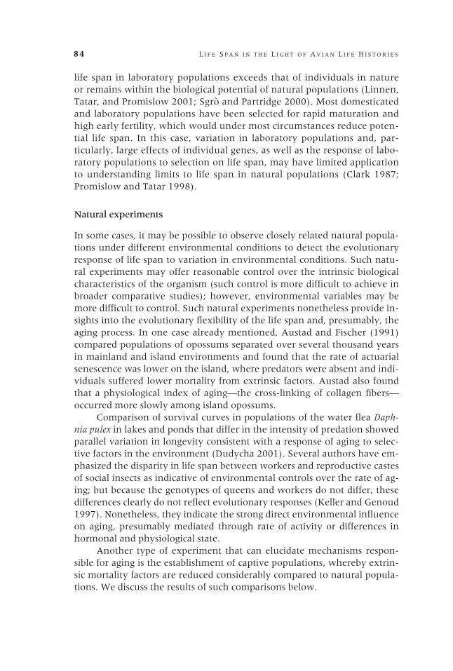
84 L I F E S P A N I N T H E L I G H T O F A V I A N L I F E H I S T O R I E S
life span in laboratory populations exceeds that of individuals in natureor remains within the biological potential of natural populations (Linnen,Tatar, and Promislow 2001; Sgrò and Partridge 2000). Most domesticatedand laboratory populations have been selected for rapid maturation andhigh early fertility, which would under most circumstances reduce poten-tial life span. In this case, variation in laboratory populations and, par-ticularly, large effects of individual genes, as well as the response of labo-ratory populations to selection on life span, may have limited applicationto understanding limits to life span in natural populations (Clark 1987;Promislow and Tatar 1998).
Natural experiments
In some cases, it may be possible to observe closely related natural popula-tions under different environmental conditions to detect the evolutionaryresponse of life span to variation in environmental conditions. Such natu-ral experiments may offer reasonable control over the intrinsic biologicalcharacteristics of the organism (such control is more difficult to achieve inbroader comparative studies); however, environmental variables may bemore difficult to control. Such natural experiments nonetheless provide in-sights into the evolutionary flexibility of the life span and, presumably, theaging process. In one case already mentioned, Austad and Fischer (1991)compared populations of opossums separated over several thousand yearsin mainland and island environments and found that the rate of actuarialsenescence was lower on the island, where predators were absent and indi-viduals suffered lower mortality from extrinsic factors. Austad also foundthat a physiological index of aging—the cross-linking of collagen fibers—occurred more slowly among island opossums.
Comparison of survival curves in populations of the water flea Daph-nia pulex in lakes and ponds that differ in the intensity of predation showedparallel variation in longevity consistent with a response of aging to selec-tive factors in the environment (Dudycha 2001). Several authors have em-phasized the disparity in life span between workers and reproductive castesof social insects as indicative of environmental controls over the rate of ag-ing; but because the genotypes of queens and workers do not differ, thesedifferences clearly do not reflect evolutionary responses (Keller and Genoud1997). Nonetheless, they indicate the strong direct environmental influenceon aging, presumably mediated through rate of activity or differences inhormonal and physiological state.
Another type of experiment that can elucidate mechanisms respon-sible for aging is the establishment of captive populations, whereby extrin-sic mortality factors are reduced considerably compared to natural popula-tions. We discuss the results of such comparisons below.
PDR 29 Supp Ricklefs.sp 7/6/06, 3:18 PM84

R O B E R T E . R I C K L E F S / A L E X S C H E U E R L E I N 85
Patterns of life-history variation involvinglife span
Until recently, most empirical studies of variation in longevity were basedon maximum reported life span. When organisms exhibit an increase inmortality rate with age and a natural population is sampled for a sufficientperiod to cover the maximum natural life span, simulated data show thatthe maximum reported life span is highly correlated with aging parametersof Gompertz and Weibull models of aging (Ricklefs and Scheuerlein 2002;Scheuerlein and Ricklefs unpubl.). Problems arise primarily when studiesare too brief. For example, among the maximum reported life spans in Careyand Judge’s (2000) thorough compilation, those for red-legged kittiwakes(4 years) and Townsend’s shearwater (5.1 years) are barely long enoughfor these seabirds to attain maturity.9 Although the data must be viewedcautiously, life span analyses nevertheless reveal general patterns in the rateof aging among animals.
Body mass
Biologists have recognized for many years that maximum potential life spanin birds and mammals is closely related to body size (Comfort 1979; Finch1990). Large animals live longer (Austad and Fischer 1991; Calder 1983,1984, 1985; Sacher 1959). This has been attributed to several causes. First,many physiological parameters, such as metabolism, development rate, andfecundity, vary with body size. Large animals have a slow rate of living,and long life may express this general property. Reduced metabolism mayalso result in reduced concentrations of reactive forms of oxygen, therebyslowing the aging process (e.g., Barja and Herrero 2000). Another conse-quence of large body size is a lower extrinsic mortality rate. Larger animalsare better able to avoid encounters with predators, and their bodies are alsobetter buffered against vagaries in the environment.
Second, it is well understood that greater survival in the face of ex-trinsic factors increases the strength of selection on life span, leading to ademographic or life-history connection between body size and rate of ag-ing. Several authors have examined this demographic connection directlyby relating aging parameters of Gompertz or Weibull functions to the esti-mated extrinsic mortality rate. As mentioned previously, Promislow (1991)compared the aging parameter g of the Gompertz equation to an estimateof the minimum mortality rate of young adults but found no relationshipbetween them. In contrast, Ricklefs (1998) found a strong relationship be-tween the derived aging parameter w and the fitted initial mortality rate(m
0) of the Weibull equation. This discrepancy raises a fundamental issue
concerning the proper definition of the rate of aging. Using the Gompertz g,
PDR 29 Supp Ricklefs.sp 7/6/06, 3:18 PM85

86 L I F E S P A N I N T H E L I G H T O F A V I A N L I F E H I S T O R I E S
one defines aging as the exponential rate of increase in mortality with age.Using w derived from either the Gompertz or Weibull equation, one definesaging according to the magnitude of the mortality rate at a particular age.In the case of the Gompertz function, the magnitude of the mortality ratedepends on both m
0 and g, hence it is difficult to separate their effects.
Multiple regression shows that the Weibull w varies with the initialmortality rate independently of the relationship of both to body size, therebymaking the demographic connection between extrinsic mortality and rateof aging more plausible and the direct allometric physiological connectionbetween size and m
x less plausible. This is further substantiated by compari-
sons between birds and mammals. For individuals of a given body size, birdshave longer life spans than mammals, perhaps by an average factor of 2–3times (Calder 1983; Holmes and Austad 1995a). When birds and mammalsare analyzed together, the rate of aging w is related to the initial mortalityrate m
0 independently of body size or of differences between birds and mam-
mals (Ricklefs 1998). Accordingly, the difference in longevity between birdsand mammals of the same body size is statistically associated with the greaterability of birds to escape mortality factors, as shown by their lower valuesof m
0. This observation strengthens the idea that the rate of aging is evolu-
tionarily flexible rather than being tied closely to other aspects of physiol-ogy, such as the rate of metabolism (Holmes and Austad 1995a, b).
Brain mass
Life span has been related to other attributes besides body mass. Brain mass,in particular, has captured the attention of comparative biologists, perhapsbecause the brain is considered the pacemaker of life in general and is theorgan that most resists aging-related change. Sacher (1959, 1978) found agood correlation between life span and brain mass for mammals, and Allmanet al. (1993) have explored this relationship in more detail for primates.However, the brain–life span relationship was questioned by Economos(1980a, b), who pointed out that brain mass is not uniquely highly corre-lated with longevity, given the strong intercorrelations, for example, be-tween brain mass and body mass. Why mass itself should exercise a domi-nant influence over life span is also not clear. Ricklefs and Scheuerlein(2001), comparing the Weibull parameter w to both body mass and brainmass in birds in a multiple regression, found that only brain mass wasuniquely related to rate of aging. Clearly, however, in comparisons involv-ing both birds and mammals, brain mass does not explain as much of thevariation in life span or rate of aging as extrinsic mortality. Thus, it is likelythat the correlation observed within either class between brain mass andlife span reflects some aspect of the ecology of species that is expressed in-dependently in both brain mass and extrinsic mortality.
PDR 29 Supp Ricklefs.sp 7/6/06, 3:18 PM86

R O B E R T E . R I C K L E F S / A L E X S C H E U E R L E I N 87
Genome size
Another attribute that has been linked to longevity is the size of the ge-nome. Although the two do not appear to be related in mammals (see Finch1990), Monaghan and Metcalfe (2000) have recently made such a claim forbirds based on independent contrasts calculated from phylogenetic relation-ships among avian families (Sibley and Ahlquist 1990). Ricklefs andScheuerlein (2001) and Morand and Ricklefs (2001) failed to find a rela-tionship between the Weibull aging parameter w and genome size in a cor-relation among terminal taxa at the species level. However, a hierarchicalanalysis of covariance based on Monaghan and Metcalfe’s data reveals astrong correlation between life span and genome size at the level of familieswithin orders but no correlation at the level of species within genera (Table 1).Even though the family-level correlation is significant, the amount of thetotal variance that resides at this taxonomic level is relatively small, henceit is hard to attach a biological meaning to the correlation. Indeed, whenthe data were partitioned into equal halves, only one of the two data setsretained a significant correlation between life span and genome size at thefamily level. This suggests that the significant correlation may have resultedfrom a chance association of data rather than an underlying mechanisticconnection between the two.
A broader life-history perspective
Ricklefs and Scheuerlein (2001) investigated life-history correlations of therate of aging (w) in birds and mammals separately. The rate of aging wasgenerally inversely related to body size, brain size (tested only for birds),and rate of postnatal development (significant only for mammals), and wasdirectly related to the lengths of incubation (birds) or gestation periods(mammals). When the independent variables were treated together in amultiple regression, only brain mass (birds) and postnatal growth rate (mam-
TABLE 1 Distribution of variance components in lifespan, genome size, and their correlation among birdsover nested taxonomic levels
Taxonomic level Life span Genome size Correlation
Order 0 0 0.00Family 26 6 1.59Genus 74 94 0.02
Total 100 100 —
NOTE: Life span is the maximum recorded value and is subject to considerable error;correlations exceeding 1.0 are possible because variance components are estimates.SOURCE: Data are from Monaghan and Metcalfe (2000) as analyzed by Morand and Ricklefs(2001); based on 67 species.
PDR 29 Supp Ricklefs.sp 7/6/06, 3:18 PM87

88 L I F E S P A N I N T H E L I G H T O F A V I A N L I F E H I S T O R I E S
mals) were uniquely related to rate of aging. Hierarchical analysis of vari-ance for life-history and aging traits of birds reveals differences in the distri-bution of variation related to the evolutionary responsiveness of each ofthe traits (Table 2). In particular, about 80 percent of the variance in em-bryonic and postnatal growth rates resides at the level of orders and fami-lies, reflecting body size differences between large taxonomic groups anddifferences in mode of development (i.e., altricial versus precocial) that in-fluence growth rate (Starck and Ricklefs 1998). Variance in mass itself isabout equally distributed between higher and lower taxonomic levels,whereas the variance in initial mortality and rate of aging is more heavilyweighted toward the taxonomic level of genus. For the smaller number ofspecies for which brain masses are available, variance in brain mass is con-centrated at the level of genus, as is the variance in rate of aging.
Variance component correlations relating the rate of aging w to otherlife-history traits show consistent significant correlations between rate of ag-ing and extrinsic mortality at the level of orders and genera within families,but correlations with body mass and incubation period are weaker (Table 3).
TABLE 3 Variance component correlations for the rateof aging (wwwww) and initial mortality rate (m0), mass, andincubation period in birds
wwwww wwwww Mass wwwww versusTaxonomic versus versus versus incubationlevel mass m0 m0 period
Order –0.41 1.10 0.59 –0.67Family 0.00 0.00 –0.80 0.00Genus –0.84 0.76 –0.92 –0.56Species –0.19 0.33 –0.51 –0.31
SOURCE: Data from Ricklefs and Scheuerlein (2001).
TABLE 2 Distribution of variance components in life-history traitsand aging parameters of birds over nested taxonomic levels
InitialTaxonomic Incubation Growth mortality Rate oflevel Mass Brain period rate (m0) aging (wwwww)
Order 42 20 47 80 10 25Family 1 0 41 0 21 0Genus 52 76 9 20 49 61Species 5 4 4 0 21 14
Total 100 100 100 100 100 100
NOTE: Variance components are estimates based on the hierarchical structure of mean squares in a nestedanalysis of variance. When the data are poorly balanced, as in analyses of this type, mean squares may decreasefrom one level to the next higher level, resulting in a negative variance component, which is arbitrarily set tozero.SOURCE: Data from Ricklefs and Scheuerlein (2001), based on 53 species.
PDR 29 Supp Ricklefs.sp 7/6/06, 3:18 PM88

R O B E R T E . R I C K L E F S / A L E X S C H E U E R L E I N 89
Comparisons between wild and captive populations
When individuals are brought into captivity, the rate of extrinsic mortalityis reduced considerably, except perhaps for the incidence of stress-relatedand contagious disease. If the increase in mortality with age resulted fromincreasing vulnerability to extrinsic mortality factors, then one would ex-pect animals in captivity to exhibit lower mortality rates at older ages thanthey do in the wild. If aging-related mortality were caused by intrinsic fac-tors that kill independently of external causes (even though the latter mayhasten intrinsically caused death), then aging-related mortality would notdiffer between captive and wild populations. Comparing wild and captivepopulations is complicated by the fact that ages at death are often estimatedby different methods, and mortality rates of young adults in captivity mayhave additional causes related to stress and contagion that are not promi-nent in the wild. Thus, such comparisons must be made with caution.
Using phylogenetically controlled comparisons, Ricklefs (2000b)showed that captive populations of birds had lower initial mortality (m
0)
but comparable rates of aging (w) vis-à-vis wild populations. This suggestedthat the Weibull model of aging, which separates extrinsic and intrinsiccauses of death in additive terms, provides a reasonable demographic de-scription of the aging process. A similar comparison of taxonomicallymatched wild and captive populations of mammals suggested in contrastthat the Weibull rate of aging decreases in captivity by an amount ex-pected of the multiplicative Gompertz model (Ricklefs and Scheuerlein2001). This result was particularly striking for mammals of open savannahabitats, for which survival rate must be closely tied to speed and endur-ance. For such species, physiological decline would seemingly lead to highervulnerability to extrinsic mortality factors, particularly predation. Preda-tors themselves should be similarly afflicted by physiological decline, andit is perhaps relevant that the lion Panthera leo shows a pattern of reducedaging-related mortality in captivity, as do several ungulates that are po-tentially its prey.10
Discussion
Comparative analyses of the rate of aging in the context of life historieshave provided insights into the aging process while leaving many issuesunresolved. In the case of birds, which are long lived compared to mam-mals of the same size, comparisons between wild and zoo populations sug-gest that the Weibull model provides a better description of the aging pro-cess than the Gompertz model. Causes of aging-related deaths are apparentlyunrelated to extrinsic mortality factors; accordingly, an additive model ofextrinsic and intrinsic mortality, such as the Weibull function, is appropri-
PDR 29 Supp Ricklefs.sp 7/6/06, 3:18 PM89

90 L I F E S P A N I N T H E L I G H T O F A V I A N L I F E H I S T O R I E S
ate. Comparison of rates of aging with body size and the extrinsic (initial)mortality rate indicates that the rate of aging responds to selection based onthe demography of a population rather than on physiological characteris-tics of individuals. Thus, for the most part, evolutionary theories of agingare supported by comparative studies. Moreover, comparisons between natu-ral and captive populations indicate that birds in the wild do not die be-cause of increasing vulnerability to extrinsic causes. This suggests that indi-vidual birds maintain high fitness late into life and that the increase inmortality with age is due to the increasing probability of catastrophic causesof death, such as cancer and stroke. The increasing proportion of aging-related deaths in populations with a large proportion of old individuals fur-ther suggests that there are inherent biological limitations on the control ofintrinsic aging-related mortality.
Correlations of the rate of aging with life-history attributes other thanextrinsic mortality are not particularly informative because of the strongcorrelations among independent variables. By considering mammals andbirds together, however, one can break this pattern of intercorrelation be-cause the different life styles of birds and mammals result in contrastingpatterns of extrinsic mortality. Thus, although the rate of aging is related tobody size and other correlated life-history attributes within both birds andmammals, analyses involving both groups clearly tie the rate of aging toextrinsic mortality. Accordingly, the rate of aging appears to be responsiveto selection on traits that extend life span or modify the rate of increase inmortality. Because the rate of aging varies in response to the demographicenvironment of a population, we may infer that postponing aging imposesa fitness cost, although the mechanisms involved are not understood. Be-cause the proportion of aging-related mortality increases with maximumpotential life span, this cost evidently increases as senescence is delayed fur-ther. Moreover, the difference in the rate of aging between birds and mam-mals of the same body size is not due to some fundamental biological dif-ference between the two groups of organisms. Rather, it is related to thefitness benefits of delayed aging, which are lower for mammals owing totheir higher extrinsic mortality rates.
The nature of the fitness cost of postponing aging (Abrams 1991) is notevident in comparative analyses. In general, increasing body size is associatedwith a reduced rate of aging, reduced extrinsic mortality, lower fecundityresulting from smaller brood size and longer development, and a higher pre-reproductive survival rate. If postponing senescence imposes a cost in termsof early fecundity or survival, this might be obscured either by contrasting orsupplementing contributions to fertility and survival from other factors. Forexample, there are many reasons, related to lower metabolic intensity andslower life processes, why larger organisms might have lower fecundity thansmaller organisms besides the costs of delayed senescence.
PDR 29 Supp Ricklefs.sp 7/6/06, 3:18 PM90

R O B E R T E . R I C K L E F S / A L E X S C H E U E R L E I N 91
Comparative analyses of life histories might provide more informationconcerning mechanisms of delayed senescence if they were applied in con-junction with mechanistic models of control of the aging process (Abramsand Ludwig 1995). For example, Ricklefs (1992, 1993) suggested that varia-tion in the development period among birds of the same body size mightinvolve mechanisms to prolong life through production of a better immunesystem or a larger, more complex nervous system. In this case, one couldsearch for a direct correlation between the rate of aging and the develop-ment rate, where the latter was sufficiently uncoupled from body size topermit separation of the two effects statistically. To the extent that suchanalyses have been performed for birds and mammals, they are consistentin that a longer development period is associated with lower extrinsic mor-tality and longer life span independently of body size (Ricklefs 1993). Clearly,slow development reduces fitness because it extends the period of exposureof highly vulnerable offspring to extrinsic mortality factors. The size of thisfitness impact can be estimated from mortality rates of parents and offspringduring the development period. If prolongation of life span were achievedby reducing fertility, one might be able to use comparative analyses to iden-tify associated adaptations of organisms that secondarily decrease the re-productive rate.
What the comparative analysis of aging requires most at this point isan unambiguous quantitative definition of the rate of aging; mechanisticmodels of aging to inform comparative analyses; and comparative data spe-cifically related to aging and its causes. General insights have been gainedby comparative life-history analyses of aging; however, at present these lackthe specificity to help characterize mechanisms of aging by their effects onlife-history traits. More-focused gathering of data and application of com-parative methods should help considerably in this regard.
We conclude with four general observations about life span—its na-ture, evolution, theoretical study, and future prospects.
(1) What are the nature and fundamental properties of life span? Com-parative studies of life tables do not address physiological processes directly.What they can say is that senescence leads to a continuous increase in themortality rate with age and that differences between populations reflect pri-marily the magnitude rather than the pattern of this increase. Although aspecies may have a maximum potential life span, it is clear that few indi-viduals reach this age. From the standpoint of the evolution of the agingpattern, factors that influence adult mortality throughout life determine theoverall pattern of aging-related mortality. An important issue is whetherthe demographic expression of aging results from increasing vulnerabilityto extrinsic causes of death due to reduced physiological capacity, or fromincreasing frequency of catastrophic intrinsic mortality factors, such as car-cinomas and cardiovascular disease. In birds, the relative constancy of the
PDR 29 Supp Ricklefs.sp 7/6/06, 3:18 PM91

92 L I F E S P A N I N T H E L I G H T O F A V I A N L I F E H I S T O R I E S
aging-related component of mortality when extrinsic mortality varies be-tween captive and natural populations weighs in favor of intrinsic causes.The data for mammals are less conclusive and may reflect a basic differencein the way mammals age.
(2) How does life span evolve in the context of the life history? Com-parative studies make quite clear that the primary selective factor is thelevel of extrinsic mortality. The role of other factors, such as parental careand sociality (Allman et al. 1998; Carey and Judge 2001), over and aboveextrinsic mortality, has not been evaluated quantitatively in a comparativecontext. Because most of the variance in the rate of aging resides at thelevel of genera within families, this observation suggests that the rate ofaging is relatively flexible from an evolutionary standpoint, but also thatmost of the variance in extrinsic mortality rates is expressed at this level.
(3) Why is there no theory of life span per se, notwithstanding thedominant focus on aging? From an evolutionary standpoint, one answer isthat the fitness effect of variation in life span is much smaller than the ef-fect of changes in mortality throughout adult life (Figure 6). This is becauseso few individuals in natural populations reach the maximum potential lifespan. This does not mean that life span per se is not responsive to selection;the evolutionary response also depends on genetic variation for a trait withina population. Comparative studies provide no evidence, however, that maxi-mum potential life span varies independently of changes in aging-relatedmortality throughout adult life.
(4) What is the future of the human life span? The increasing propor-tion of aging-related mortality in populations with older age structures sug-gests that natural populations have approached biological constraints limit-ing the potential length of life. Average human life span clearly has increasedgreatly in recent years, with many of the gains coming from reduced mor-tality rates in the oldest age classes (Robine et al. 1997). It is clear that thesechanges have resulted from manipulation of the environment rather thanchanges in the genetic makeup of the human population. Thousands of gen-erations of selection on natural populations of long-lived animals, such aselephants and albatrosses, have failed to reduce aging-related mortality tolow levels. Thus, it is likely that future progress in extending average hu-man life span will require either further improvement in the conditions oflife conducive to survival at old age or manipulations of the human ge-nome that exceed the genetic repertoire of natural populations. A moreimportant lesson from the study of aging in natural populations of birds isthat individuals can maintain high personal fitness to an advanced age aspart of the normal progress of aging. This lesson suggests that it may bemore fruitful to focus our attention on realizing and enhancing for humansthe potential natural quality of life of elderly individuals rather than tryingto extend life per se.
PDR 29 Supp Ricklefs.sp 7/6/06, 3:18 PM92

R O B E R T E . R I C K L E F S / A L E X S C H E U E R L E I N 93
This study was supported by NIH R03 AG16895-01 and R01 AG20263-01.
1 The failure of banding studies to detectaging-related mortality can be attributed toseveral factors. First, most banding studies withlarge sample sizes were restricted to small spe-cies with short life spans and high adult mor-tality rates, such as tits (Parus) and flycatchers(Ficedula). As shown by Ricklefs (1998), onlya small proportion of the mortality in popula-tions of this type is associated with the expres-sion of aging. Second, techniques for analyz-ing demographic data in early studies of bandreturns were not well developed and may havehad little power to detect age dependency ofthe survival rate. Recent development of maxi-mum likelihood models has made demo-graphic analysis much more sensitive (Lebre-ton et al. 1992). Third, recovery of ages atdeath from natural populations, unlike cohortanalysis, is not well suited to analysis of age-specific changes in the survival rate. This is be-cause, in populations that are sampled throughrecoveries of dead individuals, the decliningsizes of successively older age classes are bal-anced by an increasing mortality rate with age.Thus, the changes in age structure associatedwith aging are partly or completely compen-sated by change in the mortality rate, often re-sulting in a distribution of ages at deathsampled from a natural population that re-sembles a constant exponential (that is, non-senescing) decline.
2 Additional models incorporate addi-tional additive and multiplicative terms (e.g.,the Gompertz–Makeham function) or a level-ing off at high age (e.g., logistic function) tomatch observations on humans and on labo-ratory populations of flies (Carey et al. 1992;Fukui et al. 1993; Horiuchi and Wilmoth 1998;Vaupel et al. 1998). We have not used func-tions with an upper asymptote because too fewdata are available for natural populations ofbirds and mammals to reveal aging plateaus,and we wished to keep the number of agingparameters small to facilitate comparisonsamong taxa. Note also that the Gompertz–Makeham function,
mx = m
0 + A
0egt,
incorporates an additive term for initial mor-tality rate, but, as in the Gompertz equation,the aging-related mortality term remains anexponential increase in a portion (A
0) of the
initial mortality. Thus, it does not provide theindependence between initial and aging-re-lated mortality that the Weibull function does.
3 Specifically, w is the value of the aging-dependent mortality term axb obtained whenx = 1/w. From the logarithmic form of the ex-pression, logw = loga /(b + 1), one can see thatfor a given value of b, the value of logw is di-rectly proportional to loga. Empirically, b av-erages about 3 in bird and mammal popula-tions.
4 Application of this equation involvesmany assumptions, most notably that the lifetable of the population is constant over timeand that males and females are demographi-cally indistinguishable. When survival and fer-tility vary stochastically over time, selectiongenerally favors longer life (lower adult mor-tality) over reproduction (Hastings and Caswell1979; Schaffer 1974). For a constant life table,the change in fitness resulting from a changein any life table entry, i.e., fertility or survivalrate at a particular age, can be obtained by dif-ferentiating the equation to find dl/ds
x or dl/
dbx (Hamilton 1966). However, as Abrams
(1991, 1993) has pointed out, genetic changesinfluencing the aging process typically have anage at onset and affect life table values at allsubsequent ages. These considerations compli-cate the application of the Euler–Lotka equa-tion to the evolution of aging. Nevertheless, ithas heuristic value for exploring the effects ofchanges in life table variables on evolutionaryfitness, which can be illustrated by the simpleapproach taken here.
5 Because populations are maintained inan approximate equilibrium by density-depen-dent factors, this equation can be simplified byassuming l = 1, at which point recruitment ofyoung individuals into the breeding popula-tion (SaB) can be replaced by
S BS
Sa z a
=-
- - +
1
1 1.
6 The estimated fitness value of extend-ing average life span also shows how much
Notes
PDR 29 Supp Ricklefs.sp 7/6/06, 3:18 PM93

94 L I F E S P A N I N T H E L I G H T O F A V I A N L I F E H I S T O R I E S
mechanisms for extending life cost in terms oflife table values. In the simple model presentedabove, costs may be expressed as an increasein age at maturity (a), decrease in prerepro-ductive mortality (increase in S
a), decrease in
fertility (B), or any combination of these. Forexample, suppose life span were extended bysome mechanism that lengthened the devel-opment period. This would incur a cost interms of the reduced survival (expressed aslower B or S
a) resulting from a longer period
of exposure of the more vulnerable offspringto extrinsic mortality factors. In tropical birds,for example, daily rates of nest predation com-monly exceed 5 percent, hence extending de-velopment even for a few days, as so manytropical species do, can be very costly.
7 The technique of independent contrastsused to correct for phylogenetic relationship(Garland et al. 1992; Harvey and Pagel 1991)requires estimation of the character values orstates of ancestral nodes and thus shifts theproblem of independence to a problem of es-timation. Restricting comparisons to terminalpairs of species (sister-taxon comparisons)eliminates the problem of independence anddoes not rely on estimation of ancestral states,but results in a considerable reduction ofsample size. For example, in a sample of 20taxa, the number of independent contrasts is19, while the maximum number of sister-taxon comparisons is 10 or fewer. However,results based on independent contrasts and re-sults based on terminal taxa rarely differ quali-tatively and generally are similar quantitatively(Price 1997; Ricklefs and Starck 1996).
8 One assumption of this approach is thattaxonomic ranks are homogeneous throughouta phylogeny. In the case of birds, Sibley andAhlquist (1990) have defined taxonomic cat-egories on the basis of genetic divergence esti-mated by DNA hybridization. Genetic differ-ences are expressed as difference in the meltingpoint temperatures of homoduplexed andheteroduplexed DNA (DT
H50, ∞C). Thus, for ex-
ample, families include taxa descending from asingle ancestral node at a depth of 9–11 ∞C.
9 Most data on maximum life span fornatural populations of animals come frombirds, which have been the subjects of band-ing programs for many years. When birds are
fitted with an individually numbered leg bandas chicks or in the first year of life, when agecan be assessed by plumage, age at death canbe determined. Ages at death in mammalpopulations are based primarily on patterns ofgrowth or tooth wear and are therefore lessaccurate than those for birds. In some cases,long-term studies of individually recognizablemammals have provided more accurate demo-graphic information in natural populations(Gaillard et al. 1994).
10 One nagging feature of captive popu-lations is the relatively high “extrinsic” mor-tality rate in the absence of most extrinsic mor-tality factors. We suggest that relatively highvalues of m
0 are related to the stress of the zoo
environment, which may impair immune sys-tem function and render zoo animals morevulnerable to infection and other stress-relatedcauses of mortality in young adults. The higherrate of initial mortality may also result in alower apparent rate of aging as an artifact. Thisresult might be particularly pronounced if thehigh initial mortality rate of captive popula-tions actually decreased with age. We havetested the idea that stress might be related tohigh initial mortality in captive populations bycomparing captive populations of wild specieswith those of domesticated species, which pre-sumably have been selected for reduced stressresponse to the conditions of captivity(Scheuerlein and Ricklefs, unpubl.). Prelimi-nary results show that initial mortality of do-mesticated populations is very low, but thatthe rate of aging (w) differs little from that ofcomparable wild or captive populations. Thus,it seems plausible that captivity and domesti-cation have reduced extrinsic mortality con-siderably, but that the pattern of actuarial se-nescence has changed little. This result iscontrary to Austad’s (1993) observation thatan insular population of opossums isolatedfrom the mainland for about 4,000 years (i.e.,similar to the period of domestication of dogsand livestock) exhibited both reduced extrin-sic mortality and slower aging-related increasein mortality. The result with domesticatedmammals also reinforces the idea that the ad-ditive terms of the Weibull function portraythe underlying causes of actuarial senescencemore realistically than the multiplicative termsof the Gompertz equation.
PDR 29 Supp Ricklefs.sp 7/6/06, 3:18 PM94

R O B E R T E . R I C K L E F S / A L E X S C H E U E R L E I N 95
References
Abrams, P. A. 1991. “The fitness costs of senescence: The evolutionary importance of eventsin early adult life,” Evolutionary Ecology 5: 343–360.
———. 1993. “Does increased mortality favor the evolution of more rapid senescence?”Evolution 47: 877–887.
Abrams, P. A., and D. Ludwig. 1995. “Optimality theory, Gompertz’ law, and the dispos-able soma theory of senescence,” Evolution 49: 1055–1066.
Alexander, R. D. 1974. “The evolution of social behavior,” Annual Review of Ecology and Sys-tematics 5: 325–383.
Allman, J., T. McLaughlin, and A. Hakeem. 1993. “Brain weight and life-span in primatespecies,” Proceedings of the National Academy of Sciences USA 90: 118–122.
Allman, J., A. Rosin, R. Kumar, and A. Hasenstaub. 1998. “Parenting and survival in an-thropoid primates: Caretakers live longer,” Proceedings of the National Academy of Sci-ences USA 95: 6866–6869.
Alvarez, H. P. 2000. “Grandmother hypothesis and primate life histories,” American Journalof Physical Anthropology 113: 435–450.
Armitage, P. and R. Doll. 1954. “The age distribution of cancer and a multi-stage theory ofcarcinogenesis,” British Journal of Cancer 8: 1–12.
———. 1961. “Stochastic models for carcinogenesis,” Proceedings of the Fourth Berkeley Sym-posium on Mathematical Statistics and Probability 4: 19–38.
Arnold, S. J. 1983. “Morphology, performance and fitness,” American Zoologist 23: 347–361.Austad, S. N. 1993. “The comparative perspective and choice of animal models in aging
research,” Aging-Clinical and Experimental Research 5: 259–267.———. 1997. “Comparative aging and life histories in mammals,” Experimental Gerontology
32: 23–38.Austad, S. N. and K. E. Fischer. 1991. “Mammalian aging, metabolism, and ecology: Evi-
dence from the bats and marsupials,” Journal of Gerontology: Biological Sciences 46: B47–B53.
Barja, G. and A. Herrero. 2000. “Oxidative damage to mitochondrial DNA is inversely re-lated to maximum life span in the heart and brain of mammals,” FASEB Journal 14:312–318.
Bell, G. 1989. “A comparative method,” American Naturalist 133: 553–571.Bennett, P. M. and P. H. Harvey. 1985. “Brain size, development and metabolism in birds
and mammals,” Journal of Zoology 207: 491–509.———. 1987. “Active and resting metabolism in birds: Allometry, phylogeny and ecology,”
Journal of Zoology 213: 327–363.Botkin, D. B. and R. S. Miller. 1974. “Mortality rates and survival of birds,” American Natu-
ralist 108: 181–192.Calder, W. A., III. 1983. “Body size, mortality, and longevity,” Journal of Theoretical Biology
102: 135–144.———. 1984. Size, Function, and Life History. Cambridge, MA.: Harvard University Press.———. 1985. “The comparative biology of longevity and lifetime energetics,” Experimental
Gerontology 20: 161–170.Carey, J. R. and D. S. Judge. 2000. Longevity Records: Life Spans of Mammals, Birds, Amphib-
ians, Reptiles, and Fish. Odense, Denmark: Odense University Press.———. 2001. “Principles of biodemography with special reference to human longevity,”
Population: An English Selection 13: 9–40.Carey, J. R., P. Liedo, D. Orozco, and J. W. Vaupel. 1992. “Slowing of mortality rates at
older ages in large medfly cohorts,” Science 258: 457–461.Caruso, C. et al. 2000. “HLA, aging, and longevity: A critical reappraisal,” Human Immunol-
ogy 61: 942–949.
PDR 29 Supp Ricklefs.sp 7/6/06, 3:18 PM95

96 L I F E S P A N I N T H E L I G H T O F A V I A N L I F E H I S T O R I E S
Charlesworth, B. 1994. Evolution in Age-structured Populations, 2nd edition. Cambridge: Cam-bridge University Press.
Clark, A. G. 1987. “Senescence and the genetic correlation hang-up,” American Naturalist129: 932–940.
Comfort, A. 1979. The Biology of Senescence, 3rd ed. Edinburgh and London: ChurchillLivingstone.
Curio, E. 1989. “Is avian mortality preprogrammed?” Trends in Ecology and Evolution 4: 81–82.Derrickson, E. M. and R. E. Ricklefs. 1988. “Taxon-dependent diversification of life histo-
ries and the perception of phylogenetic constraints,” Functional Ecology 2: 417–423.Dudycha, J. L. 2001. “The senescence of Daphnia from risky and safe habitats,” Ecology Let-
ters 4: 102–105.Economos, A. C. 1980a. “Brain-life span conjecture: A re-evaluation of the evidence,” Ger-
ontology 26: 82–89.———. 1980b. “Taxonomic differences in the mammalian life span-body weight relation-
ship and the problem of brain weight,” Gerontology 26: 90–98.Edney, E. B. and R. W. Gill. 1968. “Evolution of senescence and specific longevity,” Nature
220: 281–282.Finch, C. E. 1990. Longevity, Senescence, and the Genome. Chicago: University of Chicago Press.Finch, C.E., M.C. Pike, and M. Witten. 1990. “Slow mortality rate accelerations during ag-
ing in some animals approximate that of humans,” Science 249: 902–905.Finkel, T. and N. J. Holbrook. 2000. “Oxidants, oxidative stress and the biology of ageing,”
Nature 408: 239–247.Fukui, H. H., L. Xiu, and J. W. Curtsinger. 1993. “Slowing of age-specific mortality rates in
Drosophila melanogaster,” Experimental Gerontology 28: 585–599.Gaillard, J. M., D. Allaine, D. Pontier, N. G. Yoccoz, and D. E. L. Promislow. 1994. “Senes-
cence in natural populations of mammals: A reanalysis,” Evolution 48: 509–516.Garland, T., Jr., P. H. Harvey, and A. R. Ives. 1992. “Procedures for the analysis of com-
parative data using phylogenetically independent contrasts,” Systematic Biology 41: 18–32.
Gavrilov, L. A. and N. S. Gavrilova. 1991. The Biology of Life Span: A Quantitative Approach.New York: Harwood Academic Publishers.
Hamilton, W. D. 1966. “The moulding of senescence by natural selection,” Journal of Theo-retical Biology 12: 12–45.
Harshman, L. G., K. M. Moore, M. A. Sty, and M. M. Magwire. 1999. “Stress resistance andlongevity in selected lines of Drosophila melanogaster,” Neurobiology of Aging 20: 521–529.
Harvey, P. H. and M. S. Pagel. 1991. The Comparative Method in Evolutionary Biology. Cam-bridge: Cambridge University Press.
Hastings, A. and H. Caswell. 1979. “Role of environmental variability in the evolution oflife history strategies,” Proceedings of the National Academy of Sciences USA 76: 4700–4703.
Hawkes, K., J. F. O’Connell, N. G. B. Jones, H. Alvarez, and E. L. Charnov. 1998. “Grand-mothering, menopause, and the evolution of human life histories,” Proceedings of theNational Academy of Sciences USA 95: 1336–1339.
Hayflick, L. 2000. “New approaches to old age,” Nature 403: 365.Holmes, D. J. and S. N. Austad. 1995a. “Birds as animal models for the comparative biology
of aging: A prospectus,” Journal of Gerontology: Biological Sciences 50A: B59–B66.———. 1995b. “The evolution of avian senescence patterns: Implications for understand-
ing primary aging processes,” American Zoologist 35: 307–317.Horiuchi, S. and J. R. Wilmoth. 1997. “Age patterns of the life table aging rate for major
causes of death in Japan, 1951–1990,” Journals of Gerontology Series A—Biological Sci-ences and Medical Sciences 52: B 67–B 77.
———. 1998. “Deceleration in the age pattern of mortality at older ages,” Demography 35:391–412.
PDR 29 Supp Ricklefs.sp 7/6/06, 3:18 PM96

R O B E R T E . R I C K L E F S / A L E X S C H E U E R L E I N 97
Keller, L. and M. Genoud. 1997. “Extraordinary lifespans in ants: A test of evolutionarytheories of ageing,” Nature 389: 958–960.
Kirkwood, T. B. L. 1990. “The disposable soma theory of aging,” in D. E. Harrison (ed.),Genetic Effects on Aging. Caldwell, NJ: Telford Press, pp. 9–19.
Kirkwood, T. B. L. and S. N. Austad. 2000. “Why do we age?” Nature 408: 233–238.Kirkwood, T. B. L. and R. Holliday. 1979. “The evolution of ageing and longevity,” Proceed-
ings of the Royal Society of London—Series B: Biological Sciences 205: 531–546.Lack, D. 1954. The Natural Regulation of Animal Numbers. Oxford: Clarendon Press.Lebreton, J. D., K. P. Burnham, J. Clobert, and D. R. Anderson. 1992. “Modeling survival
and testing biological hypotheses using marked animals: A unified approach with casestudies,” Ecological Monographs 62: 67–118.
Linnen, C., M. Tatar, and D. Promislow. 2001. “Cultural artifacts: A comparison of senes-cence in natural, laboratory-adapted and artificially selected lines of Drosophilamelanogaster,” Evolutionary Ecology Research 3: 877–888.
Medawar, P. B. 1952. An Unsolved Problem in Biology. London: H. K Lewis.Monaghan, P. and N. B. Metcalfe. 2000. “Genome size and longevity,” Trends in Genetics 16:
331–332.Morand, S. and R. E. Ricklefs. 2001. “Genome size, longevity, and development time in
birds,” Trends in Genetics 17: 567–568.Nealen, P. M. and R. E. Ricklefs. 2001. “Early diversification of the avian brain:body rela-
tionship,” Journal of Zoology, London 253: 391–404.Partridge, L. and N. H. Barton. 1993. “Evolution of aging: Testing the theory using Droso-
phila,” Genetica 91: 89–98.Perez-Campo, R., M. Lopez-Torres, S. Cadenas, C. Rojas, and G. Barja. 1998. “The rate of
free radical production as a determinant of the rate of aging: Evidence from the com-parative approach,” Journal of Comparative Physiology—B, Biochemical, Systemic, & Envi-ronmental Physiology 168: 149–158.
Price, T. 1997. “Correlated evolution and independent contrasts,” Philosophical Transactionsof the Royal Society of London—Series B: Biological Sciences 352: 519–529.
Promislow, D. E. L. 1991. “Senescence in natural populations of mammals: A comparativestudy,” Evolution 45: 1869–1887.
———. 1994. “DNA repair and the evolution of longevity: A critical analysis,” Journal ofTheoretical Biology 170: 291–300.
Promislow, D. E. L. and P. H. Harvey. 1990. “Living fast and dying young: A comparativeanalysis of life-history variation among mammals,” Journal of Zoology 220: 417–437.
Promislow, D. E. L. and M. Tatar. 1998. “Mutation and senescence: Where genetics anddemography meet,” Genetica 103: 299–314.
Ricklefs, R. E. 1991. “Structures and transformations of life histories,” Functional Ecology 5:174–183.
———. 1992. “Embryonic development period and the prevalence of avian blood para-sites,” Proceedings of the National Academy of Sciences USA 89: 4722–4725.
———. 1993. “Sibling competition, hatching asynchrony, incubation period, and lifespanin altricial birds,” Current Ornithology 11: 199–276.
———. 1998. “Evolutionary theories of aging: Confirmation of a fundamental prediction,with implications for the genetic basis and evolution of life span,” American Naturalist152: 24–44.
———. 2000a. “Density dependence, evolutionary optimization, and the diversification ofavian life histories,” Condor 102: 9–22.
———. 2000b. “Intrinsic aging-related mortality in birds,” Journal of Avian Biology 31: 103–111.Ricklefs, R. E. and C. E. Finch. 1995. Aging: A Natural History. New York: Scientific Ameri-
can Library.Ricklefs, R. E. and P. M. Nealen. 1998. “Lineage-dependent rates of evolutionary diversifi-
cation: Analysis of bivariate ellipses,” Functional Ecology 12: 871–885.
PDR 29 Supp Ricklefs.sp 7/6/06, 3:18 PM97

98 L I F E S P A N I N T H E L I G H T O F A V I A N L I F E H I S T O R I E S
Ricklefs, R. E. and A. Scheuerlein. 2001. “Comparison of age-related mortality among birdsand mammals,” Experimental Gerontology 36: 845–857.
———. 2002. “Biological implications of the Weibull and Gompertz models of aging,” Jour-nals of Gerontology Series A—Biological Sciences and Medical Sciences 57: B69–B76.
Ricklefs, R. E. and J. M. Starck. 1996. “Applications of phylogenetically independent con-trasts: A mixed progress report,” Oikos 77: 167–172.
Robine, J.-M., J. W. Vaupel, B. Jeune, and M. Allard. 1997. Longevity: To the Limits and Be-yond. Berlin: Springer.
Roff, D. A. 1992. The Evolution of Life Histories. New York: Chapman and Hall.———. 2002. Life History Evolution. Sunderland, MA: Sinauer Associates.Rose, M. R. 1984. “Laboratory evolution of postponed senescence in Drosophila melanogaster,”
Evolution 38: 1004–1010.———. 1991. Evolutionary Biology of Aging. New York: Oxford University Press.Rose, M. R. and J. L. Graves, Jr. 1990. “Evolution of aging,” Review of Biological Research in
Aging 4: 3–14.Sacher, G. A. 1959. “Relation of lifespan to brain weight and body weight in mammals,” in
G. E. W. Wolstenholme and M. O. Connor (eds.), CIBA Foundation Colloquia on Aging.Boston: Little, Brown, pp. 115–141.
———. 1977. “Life table modification and life prolongation,” in C. E. Finch and L. Hayflick(eds.). Handbook of the Biology of Aging. New York: Van Nostrand, pp. 582–638.
———. 1978. “Evolution of longevity and survival characteristics in mammals,” in E. L.Scheider (ed.), The Genetics of Aging. New York: Plenum, pp. 151–168.
Sæther, B.-E. 1988. “Pattern of covariation between life-history traits of European birds,”Nature 331: 616–617.
Schaffer, W. M. 1974. “Optimal reproductive effort in fluctuating environments,” AmericanNaturalist 108: 783–790.
Sgrò, C. M. and L. Partridge. 2000. “Evolutionary responses of the life history of wild-caughtDrosophila melanogaster to two standard methods of laboratory culture,” American Natu-ralist 156: 341–353.
Sibley, C. G. and J. E. Ahlquist. 1990. Phylogeny and the Classification of Birds. New Haven,CT: Yale University Press.
Silbermann, R., and M. Tatar. 2000. “Reproductive costs of heat shock protein in transgenicDrosophila melanogaster,” Evolution 54: 2038–2045.
Starck, J. M. and R. E. Ricklefs. 1998. “Variation, constraint, and phylogeny: Comparativeanalysis of variation in growth,” in J. M. Starck and R. E. Ricklefs (eds.), Avian Growthand Development: Evolution within the Altricial-Precocial Spectrum. New York: Oxford Uni-versity Press, pp. 247–265.
Stearns, S. C. 1983. “The impact of size and phylogeny on patterns of covariation in the lifehistory traits of mammals,” Oikos 41: 173–187.
———. 1992. The Evolution of Life Histories. New York: Oxford University Press.Stearns, S. C. and L. Partridge. 2000. “The genetics of aging in Drosophila,” in E. Masoro and
S. Austad (eds.), Handbook of Aging, 5th ed. San Diego: Academic Press, pp. 345–360.Strehler, B. L. and A. S. Mildvan. 1960. “General theory of mortality and aging,” Science
132: 14–21.Uno, H. 1997. “Age-related pathology and biosenescent markers in captive rhesus macaques,”
Age 20: 1–13.Vaupel, J. W. et al. 1998. “Biodemographic trajectories of longevity,” Science 280: 855–860.Weinstein, B. S. and D. Ciszek. 2002. “The reserve-capacity hypothesis: Evolutionary ori-
gins and modern implications of the tradeoff between tumor-suppression and tissue-repair,” Experimental Gerontology 37: 615–627.
Williams, G. C. 1957. “Pleiotropy, natural selection and the evolution of senescence,” Evo-lution 11: 398–411.
Wilson, D. L. 1994. “The analysis of survival (mortality) data: Fitting Gompertz, Weibull,and logistic functions,” Mechanisms of Ageing and Development 74: 15–33.
PDR 29 Supp Ricklefs.sp 7/6/06, 3:18 PM98

99
Life Span Extension ofDrosophila melanogaster:Genetic and PopulationStudies
LAWRENCE G. HARSHMAN
During the past two decades, genetic studies of model organisms have beenthe most important tool underlying advances in understanding the bio-logical basis of aging and longevity. Drosophila melanogaster, the geneticist’s“fruit fly,” is a model organism because it has been the focus of geneticstudies for more than 90 years. This review argues that studies on D.melanogaster will make an especially important contribution to the field ofaging and longevity at the intersection of research on genetics, complextraits, and fly populations.
Five approaches have been used to study the genetics of longevity ofD. melanogaster: (1) laboratory selection, (2) quantitative genetics, (3)transgenic overexpression, (4) mutation analysis, and (5) measurement ofgene expression. The first two approaches attempt to decompose longevityas a complex character. The third and fourth approaches start by lookingfor major gene effects on life span. The fifth approach is emerging as part ofa major advance in technology in which the expression of almost all genesin the genome can be measured at one time.
Genetic research on aging and longevity using D. melanogaster has beenreviewed previously (Arking 1987, 1988; Arking and Dudas 1989; Rose 1991;Curtsinger et al. 1995; Tower 1996; Stearns and Partridge 2001). The presentchapter reviews the range of genetic approaches used to study aging andlife span (length of life).
Selection experiments in the laboratory
Natural selection has shaped organic evolution whereas artificial selectionis a human endeavor, usually with some utilitarian goal. Artificial selectionis typically conducted on complex traits that are controlled by multiple genes.
PDR 29 Supp Harshman.sp 7/6/06, 3:18 PM99

100 L I F E S P A N E X T E N S I O N O F D R O S O P H I L A M E L A N O G A S T E R
Generation by generation, artificial selection can progressively change themean value of a complex trait, such as longevity, in a population. The genesthat underlie the response to selection, and traits that change as correlatedresponses to selection, are of interest in the context of understanding agingand longevity.
Figure 1 shows the distribution of a trait in a population of individualsundergoing selection. When individuals from the distribution are non-rep-resentatively selected to contribute to the next generation and genetic varia-tion contributes to the trait variation in the population, there can be a ge-netic-based change in the mean value of the trait in the next generation.
Artificial or natural selection in the laboratory has been used to studya range of traits (Rose 1984; Hoffmann and Parsons 1989; Rose et al. 1990;Huey and Kingsolver 1993; Rose et al. 1996; Gibbs 1999). Selection experi-ments magnify the difference between selected populations and ancestralor unselected control populations. Large differences are easier to study; se-lection experiments facilitate investigation by increasing the signal-to-noiseratio in the comparison of selected and control (unselected) populations.
FIGURE 1 The distribution of a trait and population mean (m)
NOTES: (A) The mean of the subset of individuals used to propagate the next generation is ms. Selectionintensity (S) is a function of the difference between m and ms. (B) The response (R) to selection is defined interms of the mean trait value in the next generation (m’) and the previous generation (m).SOURCE: Hartl and Clark 1997.
PDR 29 Supp Harshman.sp 7/6/06, 3:19 PM100

L A W R E N C E G . H A R S H M A N 101
The direct response to selection is the change in the trait targeted forselection. The indirect responses to selection consist of changes in other traits.Indirect responses to selection can be informative because they indicate ge-netic correlations between traits. Such correlations can reveal traits whoseassociation with the directly selected trait was not anticipated at the begin-ning of the experiment. Moreover, genetic associations between traits canprovide circumstantial evidence about mechanisms underlying the directresponse to selection. For example, negative correlations between traits inselection experiments suggest tradeoffs (Rose et al. 1990). Tradeoffs are basedon constraints involving energy, space, hormones, or structural biology suchthat an increase in the expression of one trait results in a decrease in an-other trait. Tradeoffs are a pivotal consideration in the evolution of longev-ity and other life-history traits (Williams 1957; Stearns 1989, 1992; Reznick1985; Zera and Harshman 2001).
A great deal of D. melanogaster genetic research on longevity has beenbased on artificial selection in the laboratory. The following summary of asubset of results is designed to focus on general outcomes and provide per-spective on the pluses and minuses associated with the use of selection ex-periments to study aging and longevity.
Selection experiments on life span
Although not the first studies of this genre, two artificial selection experi-ments have had a long-term impact on the field (Rose 1984; Luckinbill etal. 1984). In each case, the mode of selection was to select flies to propa-gate the next generation using individuals that remained fertile at old ages.For example, an artificial selection experiment by Rose (1984) increasedthe age of breeding from 4-day-old adults to 28 days (generation 1), thento 35 days (generations 2 and 3), then to 42 days, and ultimately used 70-day-old adults to maintain the selected lines. The important features ofthe experimental design included a high degree of replication (5 selectedand 5 control lines), a relatively large population size in each line to miti-gate inbreeding, and a laboratory-adapted ancestral population (Rose 1984;Rose et al. 1996). The control lines were maintained using the same gen-eration time as the ancestral population, meaning that the breeders forthe next generation were young adults. Rose (1984) and Luckinbill et al.(1984) substantially increased longevity (by 50 to 100 percent) in theirselected lines. Research on their lines highlighted stress resistance as agenetic correlate of longevity.
Selection experiments provided initial evidence for a genetic relation-ship between stress resistance and longevity. Relative to control lines, theRose lines, selected for longevity, were resistant to starvation, desiccation,and ethanol fumes, as well as elevated temperature under some conditions
PDR 29 Supp Harshman.sp 7/6/06, 3:19 PM101

102 L I F E S P A N E X T E N S I O N O F D R O S O P H I L A M E L A N O G A S T E R
(Service et al. 1985). The Luckinbill set of lines provided the first evidencefor a genetic correlation between longevity and oxidative stress resistance(Arking et al. 1991). This observation was particularly significant because itprovided indirect support for the free radical theory of aging (Harman 1956),a predominant biochemical hypothesis that explains aging in terms of oxi-dative damage to macromolecules in cells (Wallace 1992; Martin et al. 1996;Johnson et al. 1999; Guarente and Kenyon 2000).
Selection experiments also provided early evidence for a genetic asso-ciation between early-age reproduction and longevity. Females from con-trol populations exhibited a relatively short life span and high early-age eggproduction, but the converse was observed for the lines selected for ex-tended longevity (Rose 1984). Selected-line females were less fecund earlyin life regardless of whether they had mated or were virgin (Service 1989).Selected-line males also exhibited reduced reproductive function early inlife compared to control-line males (Service and Fales 1993; Service andVossbrink 1996). During the course of many generations of selection, how-ever, early-age egg production evolved to become higher in the selectedthan in the control lines in some environments (Leroi et al. 1994). Thisoutcome was interesting from an evolutionary standpoint, but it raises ques-tions about the utility of the selection experiment approach because someresults can be inconsistent over time.
Ancillary selection experiments have been used to test the direct andcorrelated responses to selection. For example, direct selection for starva-tion resistance resulted in flies with extended longevity (Rose et al. 1992).However, Harshman et al. (1999) selected only for female starvation resis-tance and did not observe an increase in female or male longevity. Bothexperiments were highly replicated, but they differed in the intensity ofselection and in other design features. In general, the relevant literaturedoes not indicate consistent support for an association between starvationresistance and extended longevity in selection experiments (Harshman etal. 1999). The heterogeneity in outcomes suggests the limitations of selec-tion experiments for understanding mechanisms underlying extended lon-gevity when such experiments are conducted in isolation from other ge-netic approaches.
Synopsis of results from laboratory selectionexperiments that extend longevity
Six selection experiments that extended the life span of D. melanogaster aresummarized here. The first two have already been described (Rose 1984;Luckinbill et al. 1984). The third and fourth artificial selection experimentswere also conducted by selection for advanced age of reproduction (Par-tridge and Fowler 1992; Partridge et al. 1999). The fifth artificial selection
PDR 29 Supp Harshman.sp 7/6/06, 3:19 PM102

L A W R E N C E G . H A R S H M A N 103
experiment selected from families that exhibited relatively high mean lon-gevity (Zwann et al. 1995). The sixth experiment was based on differentialextrinsic mortality controlled by the investigators, not artificial selection forextended longevity (Stearns et al. 2000). Some lines in this experiment ex-perienced high levels of extrinsic survival and others experienced relativelylow levels. Flies from lines that experienced low extrinsic mortality becamerelatively long-lived.
As described previously, genetic correlations can provide insight intothe mechanistic underpinnings of a response to selection. The results of thesix selection experiments are summarized in Table 1 in terms of factors thatare genetically correlated (indirect responses to selection) with extendedlongevity. In some cases the correlated responses to selection were largelyconsistent. Five of six selection experiments documented that relatively lowearly-age egg production (EF) was associated with a longer life span. This isan example of a consistent response to selection; consistent indirect responsesto similar selection experiments are arguably most suitable for continuedstudy (Harshman and Hoffmann 2000a). A useful approach might be to usethe robust genetic correlations to guide the search for underlying longevityfactors (Gibbs 1999; Zera and Harshman 2001).
Analysis of selection experiments for extendedlongevity: Studies of consistent correlated responses
Stress resistance, primarily resistance to starvation and desiccation, wasidentified as a correlate of extended longevity in selected lines (Rose 1984;
TABLE 1 Life span extension: Correlated responses to selection insix experiments
SR Lip DR Gly OR DT JV EF LF Met
R > > > > > > > < > 0L 0 0 0> 0> > > < < > 0P1 na na na na na > < 0 > naP2 na na na na na 0 0 < 0 naZ 0 0 na na na 0 na < 0 naS 0 0 > na na > na < 0 0
NOTES: The six selection experiments are identified in the table using the following abbreviations: R = Rose(1984), L = Luckinbill et al. (1984), P1 = Partridge and Fowler (1992), P2 = Partridge et al. (1999), Z = Zwann etal. (1995), S = Stearns et al. (2000). Life-history traits typically have to do with development, growth, size,reproduction, and survival. The life-history traits in Table 1 are: DT = development time, JV = juvenile viability(survival rate), EF = early-life female fecundity, and LF = late-life female fecundity. Table 1 also summarizesstress resistance traits: SR = starvation resistance, DR = desiccation resistance, OR = oxidative stress resistance.The metabolic traits in Table 1 are: Lip = lipid abundance, Gly = glycogen abundance, Met = metabolic rate(respiration rate). The symbols in the text of the table indicate whether the selected lines exhibit a greater meantrait value (>) compared to the control lines, a relatively reduced mean trait value (<), marginally greater meantrait value than the control line value (0>), no statistically significant difference between selected and controllines (0), or data are not available for a particular experiment (na).
PDR 29 Supp Harshman.sp 7/6/06, 3:19 PM103

104 L I F E S P A N E X T E N S I O N O F D R O S O P H I L A M E L A N O G A S T E R
Service et al. 1985; Service 1987). However, selection for extended lon-gevity did not result in significantly increased starvation resistance in threeof the four longevity selection experiments in which a starvation assaywas conducted (Table 1). In one of these experiments, selection on thebasis of differential adult mortality did not alter starvation resistance asan indirect response, but the selection response to selection did indicatetradeoffs between early fecundity (egg production), late fecundity, andstarvation resistance that was mediated by lipid allocation (Gasser et al.2000). Desiccation resistance appears to be more consistent as a corre-lated response to selection for longevity (Table 1). Investigation of desic-cation resistance in selection lines has revealed that the selected lines havemore glycogen, store more water, and have a reduced rate of water loss,but there is no difference in water content at death in the selected andcontrol lines (Bradley et al. 1999; Graves et al. 1992; Gibbs et al. 1997;Nghiem et al. 2000). Oxidative stress resistance in the selected lines mightbe particularly important for extended longevity. Flies from Luckinbill ex-tended longevity lines (L in Table 1) have higher levels of mRNA abun-dance corresponding to a range of antioxidant defense genes that produceenzymes including superoxide dismutase (SOD), glutathione S-transferase,catalase (CAT), and xanthine dehydrogenase as well as higher levels ofCAT and SOD enzyme activity (Dudas and Arking 1995; Force et al. 1995).These results were corroborated by a reverse selection experiment (Arkinget al. 2000a), which produced data indicating a time delay in oxidativedamage of proteins and lipids in the extended longevity lines. Antioxi-dant enzymes (CAT and Cu-Zn SOD) are found on the left arm of the 3rdchromosome, and chromosome substitution studies showed that the proxi-mal part of this chromosome arm is associated with extended longevity inthe Luckinbill selected lines (Buck et al. 1993b). Arking et al. (2000a) usedthe Luckinbill et al. (1984) lines to reverse selection for longevity by tak-ing young-age breeders for a series of generations. As a correlated response,relatively elevated measurements of antioxidant enzymes decreased in con-trol line levels, but there was no significant decrease in 11 other enzymesthat play a general role in metabolism not directly linked to antioxidantdefense. Oxidative stress resistance is also present in the Rose lines, sug-gesting oxidative stress resistance might play a general role underlyingincreased life span in response to selection for extended longevity(Harshman and Haberer 2000).
Reduced early-age reproduction appears to be a consistent correlatedresponse to selection for extended longevity (Table 1). A delay in early-stage egg maturation was found to be responsible for reduced early-age re-production in the Rose extended longevity lines (Carlson et al. 1998; Carlsonand Harshman 1999). As has been described, selection experiments alsoindicate that increased stress resistance is a consistent correlated response
PDR 29 Supp Harshman.sp 7/6/06, 3:19 PM104

L A W R E N C E G . H A R S H M A N 105
to selection (Table 1). Does this imply a negative relationship between re-production and stress resistance? As an example, selection for cold resis-tance in D. melanogaster and Drosophila simulans was correlated with decreasedearly-age fecundity (Watson and Hoffmann 1996). In general, experimentsthat have selected for stress resistance have found that decreased early-agereproduction is a correlated response (reviewed in Zera and Harshman 2001).Support for this relationship also comes from phenotypic manipulation ex-periments. Stimulation of female egg production in the Rose lines resultedin decreased starvation resistance (Chippindale et al. 1996), and stimula-tion of egg production resulted in decreased oxidative stress resistance (Wanget al. 2001; Salmon et al. 2001). The loss of oxidative stress resistance as afunction of reproduction might be particularly relevant because of the rolethat oxidative damage putatively plays in aging and longevity.
An extension of metabolic life is another consistent outcome of selec-tion experiments for longevity. The rate of gas exchange by animals, theuptake of O
2 and production of CO
2 (respiration rate), is a measure of meta-
bolic activity. Metabolism generates oxygen radicals that are thought to causeaging. Therefore, aging may be an inevitable byproduct of the metabolicfunctions of life. As a relevant observation, one or more of the mutationsthat extend the life span of the worm Caenorhabditis elegans reduce the meta-bolic rate (Van Voorhies and Ward 1999).
Is reduced respiration rate associated with extended longevity in D.melanogaster selection experiments? A series of respiration rate studies onone set of extended longevity lines is summarized in Rose and Bradley(1998). When fly respiration was measured in chambers smaller than thecages used for selection, Service (1987) found relatively higher rates atyoung ages in the control (unselected) lines than in the long-lived selectedlines, but not at later ages. Djawdan et al. (1996) found no difference be-tween selected and control lines when respiration was measured in cagesused for selection. When adults from both lines were provided with supple-mentary yeast, the control-line females exhibited a slightly higher meta-bolic rate than selected-line females (Simmons and Bradley 1997). Djawdanet al. (1997) found no difference in respiration rate when the mass ofselected and control flies was adjusted by removing the weight of water,lipid, and carbohydrate. Using the Luckinbill lines (L in Table 1), Arkinget al. (1988) demonstrated that selected longevity resulted in appreciablygreater lifetime metabolic potential than measured in control lines. Thestudy by Gasser et al. (2000), S in Table 1, included a behavioral activityassay and a measurement of respiration rate; neither was reduced in thelonger-lived lines. There is little evidence that extended longevity is ge-netically correlated with reduced metabolic rate. In selected lines of D.melanogaster, longevity does not appear to be a simple byproduct of re-duced metabolism.
PDR 29 Supp Harshman.sp 7/6/06, 3:19 PM105

106 L I F E S P A N E X T E N S I O N O F D R O S O P H I L A M E L A N O G A S T E R
Analysis of selection experiments for extendedlongevity: Demography
What is the age-specific pattern of mortality in lines selected for extendedlongevity? At issue is whether selection has reduced the rate of aging orreduced the initial mortality parameter. Demographic analyses have beenconducted on the Rose and Luckinbill lines selected for extended longevity(Service et al. 1998; Pletcher et al. 2000). Service et al. (1998) used theRose selected lines and found that the age-dependent mortality rate pa-rameter was significantly smaller and the frailty parameter had a signifi-cantly smaller variance whereas the age-independent mortality parameterdid not differ between selected and control lines. Thus, there was evidencethat the Rose selected lines evolved a reduced rate of senescence (Nusbaumet al. 1996; Service et al. 1998). Pletcher et al. (2000) investigated the linesselected for extended longevity and found that differences in baseline mor-tality, compared to the age-dependent mortality parameter, accounted formost of the difference between selected and control lines. In terms of un-derstanding the potential for life span extension, it is important to knowwhether selected life span extension is based on a delay in the aging pro-cess or on reduced age-specific mortality across a range of ages. One of thedifficulties in answering this question arises from the demands of adequatesample size because mortality is uncommon among young flies and fewflies remain alive at the oldest ages.
Analysis of selection experiments for extendedlongevity: The cost of reproduction
The cost of reproduction is a demographic relationship in which currentreproduction is associated with a reduction in future reproduction and de-creased longevity (Williams 1966; Bell and Koufopanou 1986; Reznick 1985;Stearns 1989, 1992; Partridge and Sibly 1991; Carey et al. 1998). This rela-tionship has been documented in a wide variety of plants and animals (Roff1992). The cost of reproduction is so widespread that it would be appropri-ate to consider it to be a general feature of life.
To investigate the cost of reproduction, experiments were conductedon lines selected for extended longevity (Sgro and Partridge 1999). The se-lected and control lines used were genetically differentiated in terms of early-age egg reproduction (lower in the selected lines) and longevity (greater inthe selected lines). Sgro and Partridge abolished egg maturation in femalesfrom selected and control lines to determine whether this manipulation re-moved the survival-rate differences between selected and control lines. Theyablated egg production by using irradiation or introducing a sterile muta-tion. Thus, the hypothesis was tested in parallel experiments, which helpscircumvent potentially idiosyncratic results from any one experimental ma-
PDR 29 Supp Harshman.sp 7/6/06, 3:19 PM106

L A W R E N C E G . H A R S H M A N 107
nipulation. When female reproduction was ablated, age-specific survival dif-ferences between selected and control lines disappeared (Figure 2). Withimplications that extend beyond D. melanogaster, a delayed survival cost ofreproduction could play an important role in defining lifetime survival curves(Carey et al. 1998; Sgro and Partridge 1999).
The study by Sgro and Partridge (1999) produced results indicating thatone phenomenon could underlie both the acceleration of mortality (aging)and mortality deceleration at late ages. The leveling off of mortality at lateages was originally documented in medflies by Carey et al. (1992) and in D.melanogaster by Curtsinger et al. (1992). The causes of aging and of the decel-eration of mortality at advanced ages are two of the most important prob-lems in biodemography. The results of Sgro and Partridge suggest that repro-duction could underlie aging and the deceleration of mortality at late ages.The generality of this study could be tested by repeating it with different linesand with sample sizes that allow finer resolution of age-specific mortality pat-terns, especially at ages when there were few surviving flies.
Perspectives on selection experiments
Genetic correlations are the sine qua non of laboratory selection experi-ments, but they are problematic. First, what appears to be a genetic correla-tion could be due to inadvertent independent selection on two traits (co-selection). Second, genetic correlations may be based on strong biologicalconnections between traits or very indirect association. Thus, they may ormay not provide useful evidence about mechanisms that underlie the re-sponse to selection. Third, indirect responses (genetic correlations) to selec-
FIGURE 2 Age-specific female mortality of selected populations(closed circles) and control populations (open circles) of D. melanogaster
NOTE: When female reproduction was ablated by irradiation (or introduced mutation), the age-specificmortality differences between selected and control lines disappear.SOURCE: Sgro and Partridge 1999
ln (
mort
alit
y ra
te)
Age (days)
A B Mortality ratewhen femalesreproduced
Mortality rate whenfemale reproductionwas ablated

108 L I F E S P A N E X T E N S I O N O F D R O S O P H I L A M E L A N O G A S T E R
tion for extended longevity are sometimes inconsistent between experiments(Table 1; Tower 1996; Harshman and Hoffmann 2000a). This inconsistencycould stem from a number of causes including inbreeding, inappropriateassay conditions, genetic differences between base populations, variablestrength of selection in different experiments, container effects, and mul-tiple mechanisms underlying the selection response. Unfortunately, thecauses of heterogeneity between experiments are extremely difficult to sortout. In the face of this vagary, it is best to focus on consistent indirect re-sponses (robust genetic correlations among experiments) as the most im-portant targets for further research to elucidate the mechanisms underlyingresponses to selection for longevity (Harshman and Hoffmann 2000a;Harshman and Haberer 2000).
Flies from the Rose longevity-selected lines have been found to ex-hibit no greater life span than flies collected from the field and then testedfor longevity before numerous generations have passed (Promislow andTatar 1998). This fact represents a major problem for selection experimentson longevity because selection for extended longevity in the laboratorymay merely involve removal of deleterious mutant forms of genes thathave accumulated during laboratory culture (Promislow and Tatar 1998).Alternatively, if populations adapt to the laboratory by evolving a reduc-tion in life span, then laboratory selection for extended longevity is aninformative reversal of this initial adaptation. Transfer from a natural popu-lation to the laboratory environment and subsequent culture of flies inbottles resulted in reduced stress resistance, higher early-age egg produc-tion, and a shortened life span (Sgro and Partridge 2000; Hoffmann et al.2001), indicating that these traits are interrelated (Hoffmann et al. 2001).Overall, the evidence indicates that these changes are due to natural se-lection in the laboratory.
Selection experiments have been useful for identifying properties of or-ganisms whose life span has been genetically extended. And they have provenuseful for study of such phenomena as the cost of reproduction (Sgro andPartridge 1999) and oxidative stress resistance (Arking et al. 2000b). They havehad limited utility, however, in elucidating specific mechanisms (genes, sig-naling pathways, cell biology, physiology) that directly cause life span exten-sion. Quantitative genetics provides tools that could identify specific genes thatcause extended longevity in selection experiments and other populations.
Quantitative genetics
Quantitative traits are continuously distributed in a population, and mul-tiple genes determine the distribution of these traits. For such geneticallycomplex traits, statistical techniques have been developed to characterizegenetic correlations and genetic variances, to estimate the number of majorgenes controlling the distribution of a trait, and to localize regions of chro-
PDR 29 Supp Harshman.sp 7/6/06, 3:19 PM108

L A W R E N C E G . H A R S H M A N 109
mosomes that control variation in the trait. The regions are known as quan-titative trait loci (QTL). An important goal of QTL analysis is to identify thespecific genes responsible for extended longevity in populations.
Using very small sequences and the polymerase chain reaction (PCR)of DNA it is possible to amplify regions of DNA from many locations in thegenome of D. melanogaster. Curtsinger et al. 1998 used this technique (RAPD)to assess DNA variation at approximately 1,000 positions in the genome inrelation to life span. Five genomic regions had a significant effect on the lifespan of males, females, or both sexes. The largest effect was found for avariant DNA region that does not make a protein product but was associ-ated with reduced mortality at all ages.
A more common approach used to QTL map (localize in the genome)employs recombinant inbred lines (RILs). Briefly, flies from two parentallines are crossed and the hybrid offspring are crossed back to one of theparental lines through a series of generations of matings to siblings. As aconsequence, regions of chromosomes are introduced from one parentalline into an otherwise homogenous background of the second parentalline. These introduced segments can cause variation in the trait of interestamong the RILs. The location of the introduced segments can be identi-fied by variable molecular markers distributed across the genome. Asso-ciation of the trait of interest with specific genetic markers provides a wayof mapping regions of chromosomes that contribute to population varia-tion in a complex trait (Figure 3).
A series of QTL analyses of longevity have been conducted. One study,based on a set of RILs derived from laboratory lines, assayed the longevityof virgin males and females among the RIL lines (Nuzhdin et al. 1997; Leipsand Mackay 2000; Pasyukova et al. 2000; Viera et al. 2000). Nuzhdin et al.identified 5 QTLs with major effects on longevity, but these QTLs affectedlife span in only one sex or the other. Viera et al. extended the longevityassays conducted on these recombinant inbred lines by determining meanlife span at different temperatures and after heat shock. Seventeen QTLswere identified that increased life span, and they were largely specific toeach environment and sex. There was evidence for opposing effects suchthat a QTL associated with increased life span in one environment tendedto decrease life span in other environments.
A few studies have been conducted with outbred RILs. Using recom-binant inbred lines crossed to an unrelated stock (outbred), Reiwitch andNuzhdin (2002) found correspondence between female life span QTLs iden-tified in the recombinant inbred lines and outbred lines. This study mea-sured longevity with males and females held in the same container, andin this case there were no sex differences in QTLs. In Leips and Mackay(2000), the recombinant inbred lines were crossed to the ancestral linesused to produce them. The investigators studied the effect of another en-vironment, larval (juvenile) density, on adult longevity QTLs. The six sig-
PDR 29 Supp Harshman.sp 7/6/06, 3:19 PM109

110 L I F E S P A N E X T E N S I O N O F D R O S O P H I L A M E L A N O G A S T E R
nificant QTLs identified by Leips and Mackay (2000) typically extendedlife span only at one density or in one sex. Interactions were commonamong the life span QTLs, but a combination of interacting QTLs did notnecessarily result in exceptional life span. Importantly, the QTLs identi-fied by Nuzhdin et al. (1997) and Veira et al. (2000) tended to correspondto the QTLs identified in the study using relatively outbred lines (Leipsand Mackay 2000).
QTL analyses have been conducted on recombinant inbred lines de-rived from the Luckinbill et al. (1984) selection experiment for extendedlongevity. In these studies, three life span QTLs have been identified byassaying large numbers of males and females held together from each re-combinant inbred line (Curtsinger, personal communication). One of theQTLs, on chromosome 3L, confers resistance to paraquat (oxidative stress),and it maps to a region of the genome that includes a gene that metabolizesoxygen radicals (Curtsinger et al. 1998). Unlike the results of Nuzhdin et al.(1997), these life span QTLs are not sex-specific in their effects. Thus, forthe two cases in which males and females were held in the same containerduring the longevity assays, sex-specific QTLs were not found (Reiwitchand Nuzhdin 2002; Curtsinger, personal communication).
Perspectives on quantitative genetic studies of life span
A criticism of recombinant inbred lines for the characterization of QTLs isthat inbreeding exposes the effect of deleterious mutations that have accu-
Marker Trait score Chromosome (from top)
161215181081516
10110011
12345678
chromosomes
Variable genetic marker(present or absent in thiscase)
FIGURE 3 Quantitative trait loci (QTL) mapping by marker–traitassociation in recombinant inbred lines (RILs)
chromosomes
variable genetic marker (present or absent in this example)whose presence is associated with a higher trait score
ChromosomeMarker Trait score (from top)
1 16 10 12 21 15 31 18 40 10 50 8 61 15 71 16 8
PDR 29 Supp Harshman.sp 7/6/06, 3:19 PM110

L A W R E N C E G . H A R S H M A N 111
mulated in populations. However, the use of RILs is a legitimate first step ina process that can include outbred lines. Finding the genes that do extendlife span in populations is an ultimate goal, and D. melanogaster is the bestoption for such studies among the organisms that are used as models forgenetic research. The genetic toolbox available for D. melanogaster andgenomics/bioinformatics methods will expedite identification of the genesthat extend the life span of flies.
QTL analyses of extended life span in D. melanogaster selection experi-ments could be an especially informative avenue of research because meta-bolic rate apparently has not been reduced as a result of artificial selectionfor longevity. This implies that there are forms of genes that have the po-tential to extend life span without sacrificing normal metabolism and activ-ity. In general, quantitative genetics has the potential to vastly improve thepower to detect genes that cause extended longevity in D. melanogaster popu-lations. Transgenic overexpression and mutation analysis have identifiedgenes that can cause extended longevity in the laboratory.
Transgenic overexpression of candidate genes
Candidate genes are those that might have an anticipated effect on the traitof interest. Candidate genes in the present context are those that might ex-tend longevity. Foreign genes can be introduced into the genome of D.melanogaster as candidate transgenes. The goal is to alter the level of specificgene expression for the purpose of investigating gene function. Generally,transgenes are introduced into other genomes using modified transposableelements (“jumping genes”) that can insert themselves into a recipient ge-nome (Figure 4). For this purpose, a gene of interest can be combined witha modified DNA element (P element) that can integrate into a genome. Apopulation of such recombinant molecules is injected into specific cells indeveloping embryos. These cells are destined to become the germ line thatproduces eggs and sperm and eventually adult flies. After recombinant Pelement vectors are injected into embryonic germ line cells (pole cells), in-sertion into random chromosome positions can occur because of co-injec-tion with another vector that can make the enzyme (transposase) neededfor recombinant vector integration into the genome. In short, it is possibleto introduce foreign genes into the recipient genome, and the foreign genescan be transmitted from generation to generation with the rest of the chro-mosomal genetic material. Candidate genes that have extended life span byoverexpression or by mutation are presented in Table 2. In general,transgenes that extend life span are associated with stress resistance.
Two enzymes, found in a wide variety of organisms, are known tohave a mode of action that nullifies oxygen radicals. Superoxide dismutase(SOD) scavenges superoxide anions and produces hydrogen peroxide as a
PDR 29 Supp Harshman.sp 7/6/06, 3:19 PM111

112 L I F E S P A N E X T E N S I O N O F D R O S O P H I L A M E L A N O G A S T E R
byproduct. Hydrogen peroxide, also an oxidizing agent, is broken downby catalase (CAT) into molecular water and oxygen. A transgenic extracopy of a D. melanogaster CAT gene resulted in increased enzyme activity,but no increase in longevity (Orr and Sohal 1992). Transgenic over-expression of a SOD1 (CuZn SOD) gene resulted in increased resistance tooxidative stress agents and modestly increased life span in one study, butnot in another (Reveillaud et al. 1991; Orr and Sohal 1993). Simultaneousintroduction of CAT and SOD1 genes was observed to increase life span byapproximately 20 percent (Orr and Sohal 1994). However, this result hasbeen called into question because of inadequate controls for the experi-ment (Tower 1996).
One of the advantages of D. melanogaster transgenic methodology isthat it is possible to overexpress introduced genes in specific tissues or atspecific times during the life cycle. When human SOD1 was overexpressed
Foreign gene
Pelementvector
Foreign gene
derivedadults
Pole cells
Drosophila embryo
paternal
maternal
Chromosomes
NOTE: A P element is a short segment of DNA that can allow an exogenous carrier molecule with a transgene(foreign gene) to insert at random locations in the genome.
FIGURE 4 P element–mediated introduction of foreign genes
Chromosomes
paternal set
maternal set
derived adultsForeign gene
Pole cells
Drosophila embryo
Pelementvector Foreign gene
Foreign gene
PDR 29 Supp Harshman.sp 7/6/06, 3:20 PM112

L A W R E N C E G . H A R S H M A N 113
exclusively in adult motor neurons of D. melanogaster, life span was ex-tended by 40 percent (Parkes et al. 1998). As an aside, mutations in thehuman SOD1 gene are the basis of familial amyotrophic lateral sclerosis(commonly known as Lou Gehrig’s disease), which is an inherited life-shortening human disease characterized by deterioration of motor neu-rons. Sun and Tower (1999) overexpressed D. melanogaster SOD1 in adultD. melanogaster, extending life span by 48 percent. In this study, over-expression was not constrained to motor neurons. To the extent that thestudies can be compared, the life span–extending effect of SOD1 over-expression in the whole body (Sun and Tower 1999) was not much greaterthan that observed by Parkes et al. (1998). This comparison suggests thatoxidative damage to motor neurons is a major cause of aging. The DPOSHgene, also associated with stress resistance, extends longevity by 14 per-cent when expressed in the nervous system throughout the life cycle (Seonget al. 2001: Table 2). In general, cells that are not replaced by new cells inadults, such as neurons, are especially vulnerable to oxidative damage andmay play an important role in aging. Mitochondria are the major source ofoxygen radical production that may cause aging and limit life span (Wallace1992). The gene for the manganese-dependent superoxide dismutase (SOD2)is associated with mitochondria in higher organisms. SOD2 has been stablyintroduced into the genome of D. melanogaster and overexpressed, therebyextending the life span of D. melanogaster adults by approximately 50 per-cent (Sun et al. 2002).
TABLE 2 Genes that have extended the life span of D. melanogaster inthe laboratory
Genes Gene product Possible life span extension effect
Overexpression (high level of gene activity)SOD1 (CuZn) and superoxide dismutase oxidative stress resistanceSOD2 (Mn) (an enzyme)
hsp70 heat shock protein high temperature tolerance
DPOSH signaling protein stress resistance pathway activationand/or resistance to programmedcell death
Mutation (partial or total loss of gene function)mth G protein–coupled multiple stress resistance
receptor (putative)
Indy dicarboxylate reduced intermediary metabolismco-transporter (putative)
InR and chico 1 insulin receptor and altered control of metabolism andinsulin receptor docking some stress resistanceprotein
PDR 29 Supp Harshman.sp 7/6/06, 3:20 PM113

114 L I F E S P A N E X T E N S I O N O F D R O S O P H I L A M E L A N O G A S T E R
Oxidative damage, high temperature, and other factors can denatureproteins, resulting in deleterious physiological and fitness effects (Feder andHoffmann 1999). Heat shock proteins (HSP) and molecular chaperones canrefold damaged proteins. Thus, investigators tested the hypothesis that arelatively high level of HSP70 production would increase life span (Khazaeliet al. 1997; Tatar et al. 1997). For one test, two P element transgenic strainsof D. melanogaster were used (Tatar et al. 1997). One of the strains had extracopies of hsp70 genes. The second strain was very similar in having a rem-nant P element present at the same location as the extra copy strain, butthe extra copies of the hsp70 genes had been excised. When adults werebriefly exposed to high temperature, which stimulates activity of thetransgenes, flies from the high copy hsp70 strain exhibited relatively de-creased mortality rates for two weeks and a 4–8 percent increase in life span.If a high level of this heat shock protein is beneficial, why wouldn’t heatshock proteins be continuously expressed at high levels? The answer maybe that high levels of HSP70 negatively affect other parts of the life cycle.For example, overexpression of hsp70 can negatively affect larval (juvenile)flies by retarding growth, reducing viability, and reducing egg hatch (Krebsand Feder 1997, 1998; Silbermann and Tatar 2000).
Perspectives on transgenic overexpression
When transgenes are inserted into genomes, their effects can depend on theposition of insertion or on differences between genomes into which they areinserted. Overexpression studies have varied in the extent to which they havecontrolled for such effects to rule out the possibility of artifacts (Kaiser et al.1997; Stearns and Partridge 2001). The studies by Sun and Tower (1999) andSun et al. (2002) are exemplary in their controls for position and geneticbackground effects and their use of a sufficient number of replicate lines.
Mutation analysis
Mutation analysis is a preeminent analytical tool in contemporary biology.In general, new mutations are generated and screened to identify genes thataffect a biological trait of interest. The goal is to identify the underlying genescontrolling trait manifestation and the role of these genes in the process.Mutations in D. melanogaster have identified genes that can increase longev-ity. In all cases, transposable DNA (P elements) was used to induce the mu-tations (Figure 5). When a P element moves and reinserts itself elsewhere inthe genome it can cause a mutation. As opposed to transgenic overexpression,all of the mutations described in this section reduce the expression of, ortotally inactivate, specific genes (such as those included in Table 2).
PDR 29 Supp Harshman.sp 7/6/06, 3:20 PM114

L A W R E N C E G . H A R S H M A N 115
The first D. melanogaster longevity-extension mutation was in theMethuselah (mth) gene (Lin et al. 1998). The mth mutation results in partialloss of function of the gene and extends longevity by 35 percent. The mthgene produces a protein, presumably a G protein–coupled receptor, thatbelongs to a family of proteins associated with a range of functions in higherorganisms including endocrinology, neurology, and response to externalstimuli. The putative G protein product of the mth gene is not similar to anyof the G proteins of known function in other organisms, and thus the spe-cific function of the mth gene is not suggested by comparison with otherorganisms. There is evidence that the mth gene plays a role in regulation ofneuromuscular neurotransmitter function (Song et al. 2001). Again, neu-romuscular function might be especially important for aging and longevity.The mth mutation resulted in increased stress resistance (Lin et al. 1998),and the mutant flies were approximately one-third larger than controls.Mutant flies were substantially more resistant to starvation, high tempera-ture, and oxidative stress.
Mutations that markedly extend life span were also found in the Indygene (Rogina et al. 2000). Indy mutations can result in a 50 percent in-
FIGURE 5 Transposon insertional mutagenesis
Parents P+ P-
X (mating)
next generation
Post-fertilization
newmutationsin specific
genes
Adults p
Chromosomes (with many genes)
Paternal set Maternal set
or or…p
Progeny
p por orp
Parents P+ P–
NOTE: A P element transposon is a short segment of DNA that can move within the genome and cause mutations.If a male with one or more P elements is mated to a female with none, then P elements can move to newlocations in the chromosomes of the progeny, sometimes causing mutation.
Chromosomes (with many genes)
Paternal set Maternal set
X(mating)
next generation
or
or
newmutationsin specific
genes
or
or…
Post-fertilization
Adults
Progeny
p
p
p
p
p
PDR 29 Supp Harshman.sp 7/6/06, 3:20 PM115

116 L I F E S P A N E X T E N S I O N O F D R O S O P H I L A M E L A N O G A S T E R
crease in maximum longevity and approximately a twofold increase in meanlife span. Five independent mutations in the same gene were reported, eachof which exhibited a substantial increase in longevity in combination witha normal gene (as a heterozygote). Moreover, the heterozygote females,derived from crosses between a laboratory stock (Canton S) and mutantstocks, produced substantially more eggs than Canton S females (Rogina etal. 2000), but the heterozygotes derived from crosses to a more relevantcontrol strain had only slightly greater fecundity than the control strain(Helfand, personal communication).
The Indy gene product is a protein similar to mammalian dicarboxylateco-transporters. Mammalian co-transporters are membrane proteins thattransport intermediates of energy compound metabolism (Krebs cycle in-termediates) into cells. The Indy gene is expressed at high levels in the gut,fat body, and oenocytes, which are the insect tissues/cells that play a pre-dominant role in intermediary metabolism and storage of metabolic prod-ucts. A decrease in metabolic product uptake mediated by the Indy muta-tion suggests that the mechanism of life span extension could be caloricrestriction (Rogina et al. 2000), which is an environmental intervention thatcan increase life span in invertebrates and mammals.
For the purposes of experimental rigor, Indy mutations were crossedto different stocks to check longevity of the heterozygotes compared to lon-gevity of flies from the homozygote (double mutation) stocks (Rogina et al.2000). The heterozygotes were substantially longer lived in all but one case.When Indy was crossed to flies from Luckinbill selected lines (L in Table 1)there was only a 15 percent increase in longevity of the heterozygote com-pared to the selected line. This result suggests the intriguing possibility thatthe response to artificial selection for longevity includes the “Indy mecha-nism” for life span extension (Rogina et al. 2000).
Mutations in the insulin signaling pathway can also extend the lifespan of D. melanogaster (Tatar et al. 2001; Clancy et al. 2001). These resultsfollow the pioneering work using Caenorhabiditis elegans in which mutationsselected for extended life span were found in genes that encode interactingproteins (signaling pathway) that mediate the effects of insulin (Friedmanand Johnson 1988; Kenyon et al. 1993; Dorman et al. 1995; Morris et al.1996; Kimura et al. 1997; Paradis et al. 1998; Gill et al. 1999). The discov-ery of mutations in D. melanogaster that extend life span by reducing activityof the insulin signaling pathway suggests that a general mechanism under-lies differential aging and extended longevity in animals.
D. melanogaster insulin signaling mutations that extend life span wereassociated with the InR gene that encodes the insulin receptor (Tatar et al.2001). Increased female longevity resulted only from a specific combina-tion of InR mutations. Another longevity mutation was in the chico genethat encodes an insulin receptor substrate protein (Clancy et al. 2001). The
PDR 29 Supp Harshman.sp 7/6/06, 3:20 PM116

L A W R E N C E G . H A R S H M A N 117
insulin signaling pathway plays an important role in controlling growth;loss of function associated with the InR and chico mutations results in dwarfadult flies in addition to extended longevity. chico has fewer and smallercells, resulting in a body size that is 50 percent of normal (Bohni et al. 1999).chico mutants are known to have a relatively high proportion of lipid (Bohniet al. 1999), and perhaps correspondingly the chico mutant flies were foundto be starvation resistant (Clancy et al. 2001). Similarly, Tatar et al. (2001)found that higher levels of energy storage fat (triglyceride lipid) were foundthan in a comparable fly stock. Small size, stress resistance, and high levelsof lipids are to some degree associated with extended longevity of mutantCaenorhabditis, Drosophila, and mice (Clancy et al. 2001; Tatar et al. 2001).
Tatar et al. (2001) found that InR mutations conferred as much as an 85percent extension of longevity in females and reduced late-age mortality ratesin males. There was no decrease in metabolic rate of the mutant flies as mea-sured by mass-specific oxygen consumption in a mixed sample of males andfemales. Tatar et al. found that the InR mutations have approximately 25percent of normal juvenile hormone biosynthesis and interpreted this defi-ciency as a basis for increased longevity. Exogenous administration of a juve-nile hormone mimic stimulated reproductive activity in InR mutation femalesand reduced life span of the mutant toward that of the wild type control.Tatar et al. argued that the longevity associated with the InR mutations wasactually due to a deficiency in this class of insect hormone.
Clancy et al. (2001) tested mutations in various genes in the insulinsignaling pathway, including the insulin receptor gene, and found that allbut one was associated with normal or decreased longevity. Only the chico 1
mutation was found to increase male and female longevity, by up to 48percent when the mutant was present in two copies (homozygote) and 36percent when the mutant was combined with a normal gene (heterozy-gote). Resistance to elevated temperature, oxidative stress, and starvationwas tested using the chico mutation and related normal flies. Starvation re-sistance was observed for heterozygotes and homozygote mutants, oxida-tive stress resistance was observed only for heterozygotes, and no resistanceto elevated temperature was associated with the mutation. The effect ofchico on stress resistance was not as consistent as for the long-lived muta-tions that affect the insulin signaling pathway of C. elegans. For chico, thehomozygotes were half the size, but the moderately long-lived heterozy-gotes were of normal size (Clancy et al. 2001). Consequently, body size andlongevity appear to be at least partially independently determined. Heterozy-gote chico females have reduced fecundity and the homozygote was sterile.Thus, the question arose whether enhanced longevity associated with chicowas a byproduct of reduced reproduction (i.e., a reduced cost of reproduc-tion). Clancy et al. used the ovoD mutation of normal flies that were compa-rable to chico to test the hypothesis that sterility was the underlying cause
PDR 29 Supp Harshman.sp 7/6/06, 3:20 PM117

118 L I F E S P A N E X T E N S I O N O F D R O S O P H I L A M E L A N O G A S T E R
of extended longevity of chico females. chico females were found to live asubstantially longer time than sterile females that were otherwise normal.These results indicate that sterility and defective insulin signaling can ex-tend life span by different mechanisms in D. melanogaster. However, this re-sult does not exclude the possibility of an interaction between the repro-ductive system, insulin signaling, and longevity as has been observed in C.elegans (Hsin and Kenyon 1999; Lin et al. 2001).
Perspectives on mutation analysis
Mutation analysis is a form of site-localized genome perturbation performedto find genes that can extend longevity. Unlike transgenic overexpression,the outcome is not constrained by a priori expectations about which genescould produce the effect. Given this lack of constraint, it is interesting thatlong-lived mutants have reinforced the outcome of selection experimentsin identifying stress resistance as a common component of longevity. In thefuture, mutation analysis should be able to identify a range of genes thatconfer longevity in D. melanogaster. The potential for synergist studies usinglong-lived mutants and populations (lines selected for longevity) is indi-cated by the use of the Indy mutation and the Luckinbill selected lines(Rogina et al. 2000).
Gene expression
A central tenet of biology is that genes produce messenger RNA (mRNA),which in turn is used as a message to make proteins. Gene activity (expres-sion) can be measured by the amount of message (mRNA) produced by spe-cific genes or by reporter genes.
Helfand et al. (1995) and Rogina and Helfand (1995) monitored geneexpression during aging in D. melanogaster using a series of transgenic linesthat differed in the chromosomal location of P element reporter gene inser-tions in the genome. The reporter genes indicated the level of activity ofnearby genes. Age-dependent differential gene expression was documentedand related to longevity differences among lines.
Another approach has been to monitor the production of mRNA fromspecific genes as a measurement of age-dependent gene expression. For ex-ample, the abundance of mRNA corresponding to heat shock proteins hasbeen quantified as D. melanogaster ages. The abundance of heat shock pro-tein 70 (HSP70) mRNA does not increase substantially during aging (Wheeleret al. 1995), but mRNA corresponding to two smaller heat shock proteins(HSP22 and HSP23) increases markedly as a function of age (King and Tower1999). Moreover, the level of hsp22 gene mRNA was relatively high in theRose lines selected for extended longevity (Kurapati et al. 2000). However,
PDR 29 Supp Harshman.sp 7/6/06, 3:20 PM118

L A W R E N C E G . H A R S H M A N 119
overexpression of hsp22 results in decreased longevity without affecting thelevel of message production by hsp70 (Tower, personal communication).Some genes that are expressed at high levels in relatively old individualsmay simply represent loss of control of proper expression as a function ofage (Tower 1996; Guarente and Kenyon 2000). Alternatively, genes thatare highly expressed in aging flies might provide a protective function thatcould be confirmed by life span extension in transgenic overexpression stud-ies (Tower 1996, 2000).
Technology allows for simultaneous measurement of the relative amountof mRNA produced by almost all of the genes in the genome of D. melanogaster.In one study, gene expression was found to be much more strongly affectedby sex than by age (Jin et al. 2001). In another study, the investigators mea-sured expression of approximately 8,000 genes as a function of age and oxi-dative stress (Zou et al. 2000). A total of 127 genes changed expression ap-preciably during aging, and a third of these genes also responded to oxidativestress. This pattern of co-expression indicates a set of candidate genes thatcould contribute to longevity. Caloric restriction can extend the life span ofD. melanogaster. Dietary conditions that extend life span reduce the expres-sion of genes associated with growth, metabolism, reproduction, and stressresistance (Pletcher et al. 2002). In this study (Pletcher et al. 2002), almost aquarter of the genes changed in expression during the process of aging.
Perspectives on gene expression studies
Even at this early stage in application of genome-wide gene expression tech-nology (microarrays), studies have identified many changes in age-relatedgene expression potentially relevant to extended longevity. Among the ques-tions being explored are whether a few key genes control the expression ofmany other genes to extend longevity, which genes are suitable candidatesfor functional tests by transgene overexpression or techniques designed tosuppress gene activity, and whether these genes will elucidate the relation-ship between delayed early-age reproduction, stress resistance, and longev-ity in populations.
Future approaches
A theme of this review has been that the diversity of genetic approachesused to study D. melanogaster is generating considerable insight into life spanextension. Continuing this approach, powerful genetic technologies (muta-tion analysis, transgenes, genomics) combined with a rich population con-text (quantitative genetics, laboratory selection experiments, natural popu-lation studies such as Mitrovski and Hoffmann 2001) will be the basis foradvances in understanding how genes control longevity in populations.
PDR 29 Supp Harshman.sp 7/6/06, 3:20 PM119

120 L I F E S P A N E X T E N S I O N O F D R O S O P H I L A M E L A N O G A S T E R
Given that overall fitness is requisite for individuals in outbreeding popula-tions, the insight derived from studies on natural populations of flies maybe particularly applicable to the design of interventions to extend the spanof active and healthy human life.
Note
Marta Wayne kindly provided Figure 3 andRyan Baller made major contributions to Fig-ures 4 and 5. Discussions with SergeyNuzhdin, Linda Partridge, Daniel Promislow,and John Tower were valuable for this re-
view. James Curtsinger, Steven Helfand, andJohn Tower kindly provided informationfrom unpublished studies. Support for thisreview was provided by the National Insti-tute on Aging (AG08761).
References
Arking, Robert. 1987. “Genetic and environmental determinants of longevity in Drosophila,”Basic Life Sci. 42: 1–22.
———. 1988. “Genetic analyses of aging processes in Drosophila,” Exp. Aging Res. 14: 125–135.
Arking, R., S. Buck, R. A. Wells, and R. Pretzlaff. 1988. “Metabolic rates in genetically basedlong lived strains of Drosophila,” Experimental Gerontology 23: 59–76.
Arking, R., S. Buck, A. Berrios, S. Dwyer, and G. T. Baker. 1991. “Elevated antioxidantactivity can be used as a bioassay for longevity in a genetically long-lived strain ofDrosophila,” Develop. Genetics 12: 362–370.
Arking, R., V. Burde, K. Graves, R. Hari, E. Feldman, A. Zeevi, S. Soliman, A. Saraiya, S.Buck, J. Vettraino, K. Sathrasala, N. Wehr, and R. L. Levine. 2000a. “Forward andreverse selection for longevity in Drosophila is characterized by alteration of antioxi-dant gene expression and oxidative damage patterns,” Exp. Gerontol. 35: 167–185.
Arking, R., V. Burde, K. Graves, R. Hari, E. Feldman, A. Zeevi, S. Soliman, A. Saraiya, S.Buck, J. Vettraino, and K. Sathrasala. 2000b. “Identical longevity phenotypes are char-acterized by different patterns of gene expression and oxidative damage,” Exp. Gerontol.35: 353–373.
Arking, Robert and S. P. Dudas. 1989. “Review of genetic investigations into the aging pro-cesses of Drosophila,” J. Am. Geriatr. 37: 757–773.
Bell, Graham and V. Koufopanou. 1986. “The cost of reproduction,” in R. Dawkins and M.Ridley (eds.), Oxford Surveys of Evolutionary Biology. Oxford: Oxford University Press,pp. 83–131.
Bohni, R., J. Riesgo-Escovar, S. Oldham, W. Brogiolo, H. Stocker, B. F. Andruss, K.Beckingham, and E. Hafen. 1999. “Autonomous control of cell and organ size byCHICO, a Drosophila homolog of vertebrate IRS1-4,” Cell 97: 865–875.
Bradley, T. J., A. E. Williams, and M. R. Rose. 1999. “Physiological responses to selectionfor desiccation resistance in Drosophila melanogaster,” Amer. Zool. 39: 337–345.
Buck, S., M. Nicholson, S. P. Dudas, G. T. Baker III, and R. Arking. 1993a. “Larval regula-tion of adult longevity in a genetically selected long-lived strain of Drosophilamelanogaster,” Heredity 71: 23–32.
Buck, S., R. A. Wells, S. P. Dudas, G. T. Baker III, and R. Arking. 1993b. “Chromosomallocalization and regulation of the longevity determinant genes in a selected strain ofDrosophila melanogaster,” Heredity 71: 11–22.
Carey, J. R., P. Liedo, H.-G. Muller, J.-L. Wang, and J. W. Vaupel. 1998. “Dual aging modesin Mediterranean fruit fly females,” Science 281: 396–398.
PDR 29 Supp Harshman.sp 7/6/06, 3:20 PM120

L A W R E N C E G . H A R S H M A N 121
Carey, J. R., Pablo Liedo, D. Orozco, and J. W. Vaupel. 1992. “Slowing of mortality rates atolder ages in large medfly cohorts,” Science 258: 457–461.
Carlson, K. A. and L. G. Harshman. 1999. “Extended longevity lines of Drosophila melanogaster:Characterization of oocyte stage and ovariole numbers as a function of age and diet,”J. Gerontol. 54: B432–440.
Carlson, K. A., T. J. Nusbaum, M. R. Rose, and L. G. Harshman. 1998. “Oocyte maturationand ovariole numbers in lines of Drosophila melanogaster selected for postponed senes-cence,” Funct. Ecol. 52: 514–520.
Chippindale, Adam K., T. J. F. Chu, and Michael R. Rose. 1996. “Complex trade-offs andthe evolution of starvation resistance in Drosophila melanogaster,” Evolution 50: 753–766.
Clancy, D. J., D. Gems, L. G. Harshman, S. Oldham, H. Stocker, E. Hafen, S. J. Leevers, andL. Partridge. 2001. “Extension of life-span by loss of CHICO, a Drosophila insulin re-ceptor substrate protein,” Science 292: 104–106.
Curtsinger, J. W., H. H. Fukui, D. R. Townsend, and J. W. Vaupel. 1992. “Demography ofgenotypes: Failure of the limited life-span paradigm in Drosophila melanogaster,” Science258: 461–463.
Curtsinger, James W., Hidenori H. Fukui, Aziz A. Khazaeli, Andrew Kirscher, Scott D.Pletcher, Daniel E. L. Promislow, and M. Tatar. 1995. “Genetic variation and aging,”Ann. Rev. Genet. 29: 553–575.
Curtsinger, J. W., H. H Fukui, A. S. Resler, K. Kelly, and A. A. Khazaeli. 1998. “Geneticanalysis of extended life span in Drosophila melanogaster: RAPD screen for geneticdivergence between selected and control lines,” Genetica 104 : 21–32.
Djawdan, M., T. T. Sugiyama, L. K. Schlaeger, T. J. Bradley, and M. R. Rose. 1996. “Meta-bolic aspects of the trade-off between fecundity and longevity in Drosophilamelanogaster,” Physiol. Zool. 69: 1176–1195.
Djawdan, M., M. R. Rose, and T. J. Bradley. 1997. “Does selection for stress resistance lowermetabolic rate?” Ecology 78: 828–837.
Dorman, J. B., B. Albinder, T. Shroyer, and C. Kenyon. 1995. “The age-1 and daf-2 genesfunction in a common pathway to control the lifespan of Caenorhabditis elegans,” Ge-netics 141: 1399–1406.
Dudas, S. P. and R. A. Arking. 1995. “A coordinate upregulation of antioxidant gene activi-ties is associated with the delayed onset of senescence in a long-lived strain of Droso-phila,” J. Gerontol. Biol. Sci. 50A: B117–B127.
Feder, M. E. and G. E. Hoffmann. 1999. “Heat-shock proteins, molecular chaperones andthe stress response: Evolutionary and ecological physiology,” Annu. Rev. Physiol. 61:243–282.
Force, A. G., T. Staples, T. Soliman, and R. Arking. 1995. “A comparative biochemical andstress analysis of genetically selected Drosophila strains with different longevities,” Dev.Genet. 17: 340–351.
Friedman, D. B. and T. E. Johnson. 1988. “A mutation in the age-1 gene in Caenorhabditiselegans lengthens life and reduces hermaphrodite fertility,” Genetics 118: 75–86.
Gasser, M., M. Kaiser, D. Berrigan, and S. C. Stearns. 2000. “Life-history correlates of evo-lution under high and low adult mortality,” Evolution 54: 1260–1272.
Gibbs, A. G. 1999. “Laboratory selection for the comparative physiologist,” J. Exp. Biol. 202:2709–2718.
Gibbs, A. G., A. K. Chippindale, and M. R. Rose. 1997. “Physiological mechanisms of evolveddesiccation resistance in Drosophila melanogaster,” J. Exp. Biol. 200: 1821–1823.
Gill, E. B., E. M. Link, L. X. Liu, C. D. Johnson, and J. A. Lees. 1999. “Regulation of theinsulin-like developmental pathway of Caenorhabitis elegans by a homolog of the PTENtumor suppressor gene,” Proc. Natl. Acad. Sci. USA 96: 2925–2930.
Graves, J. L., E. C. Toolson, C. Jeong, L. N. Vu, and M. R. Rose. 1992. “Desiccation, flight,glycogen and postponed senescence in Drosophila melanogaster,” Physiol. Zool. 65: 268–286.
PDR 29 Supp Harshman.sp 7/6/06, 3:20 PM121

122 L I F E S P A N E X T E N S I O N O F D R O S O P H I L A M E L A N O G A S T E R
Guarente, L. and C. Kenyon. 2000. “Genetic pathways that regulate ageing in model or-ganisms,” Nature 408: 255–262.
Harman, D. 1956. “Aging: A theory based on free radical and radiation chemistry,” J. Gerontol.11: 298–300.
Harshman, L. G. and B. A. Haberer. 2000. “Oxidative stress resistance: A robust correlatedresponse to selection in extended longevity lines of Drosophila melanogaster? J. Gerontol.A Biol. Sci. Med. Sci. 55: B415–417.
Harshman, Lawrence G. and Ary A. Hoffmann. 2000a. “Laboratory selection experimentsusing Drosophila: What do they really tell us?” Trends in Ecology and Evolution 15: 32–36.
———. 2000b. “Reply from L. G. Harshman and A. A. Hoffmann,” Trends in Ecology andEvolution 15: 207.
Harshman, L. G., K. M. Moore, M. A. Sty, and M. M. Magwire. 1999. “Stress resistance andlongevity in selected lines of Drosophila melanogaster,” Neurobiol. Aging 20: 521–529.
Hartl, Daniel L. and Andrew G. Clark. 1997. Principles of Population Genetics. Sunderland,MA: Sinauer Associates.
Helfand, S. L., K. J. Blake, B. Rogina, M. D. Stracks, A. Centurion, and B. Naprta. 1995.“Temporal patterns of gene expression in the antenna of the adult Drosophilamelanogaster,” Genetics 140: 549–555.
Hoffmann, Ary A., R. Hallas, C. Sinclair, and Linda Partridge. 2001. “Rapid loss of stressresistance in Drosophila melanogaster under adaptation to laboratory culture,” Evolution52: 436–438.
Hoffmann, A. A. and P. A. Parsons. 1989. “An integrated approach to environmental stresstolerance and life history variation: Desiccation tolerance in Drosophila,” Biol. J. Linn.Soc. 37: 117–136.
Hsin, H. and C. Kenyon. 1999. “Signals from the reproductive system regulate the lifespanof C. elegans,” Nature 399: 362–366.
Huey, R. B. and J. G. Kingsolver. 1993. “Evolution of resistance to high temperature inectotherms,” Am. Nat. 142: S21–S46.
Jin, W., R. M. Riley, R. D. Wolfinger, K. P. White, G. Passador-Gurgel, and G. Gibson. 2001.“The contribution of sex, genotype and age to transcriptional variance in Drosophilamelanogaster,” Nature Genetics 29: 389–395.
Johnson, F. B., David A. Sinclair, and Leonard Guarente. 1999. “Molecular biology of ag-ing,” Cell 96: 291–302.
Kaiser, M., M. Gasser, R. Ackermann, and S. C. Stearns. 1997. “P-element inserts intransgenic lines: A cautionary tale,” Heredity 78: 1–11.
Kenyon, C., J. Chang, A. Gensch, A. Rudner, and R. Tablang. 1993. “A C. elegans mutantthat lives twice as long as wild type,” Nature 366: 461–464.
Khazaeli, A. A., M. Tatar, S. D. Pletcher, and J. W. Curtsinger. 1997. “Heat-induced longev-ity extension in Drosophila. I. Heat treatment, mortality, and thermotolerance,” Jour-nal of Gerontology, Biological Sciences 52A, B48–B52.
Kimura, K. D., H. A. Tissenbaum, Y. Liu, and G. Ruvkun. 1997. “Daf-2, an insulin receptor-like gene that regulates longevity and diapause in Caenorhabditis elegans,” Science 277:942–946.
King, V. and J. Tower. 1999. “Aging-specific expression of Drosophila hsp22,” Develop. Biol.207: 107–118.
Krebs, R. A. and M. E. Feder. 1997. “Deleterious consequences of Hsp70 overexpression inDrosophila melanogaster larvae,” Cell Stress and Chaperones 2: 60–71.
———. 1998. “Hsp70 and larval thermotolerance in Drosophila melanogaster: How much isenough and when is more too much?” Jour. Insect Physiol. 44: 1091–1101.
Kurapati, Raj, Hardip B. Passananti, Michael R. Rose, and John Tower. 2000. “Increasedhsp22 RNA levels in Drosophila lines genetically selected for increased longevity,” Jour.Gerontol. A. Biol. Sci. Med. Sci. 55: B552–B559.
PDR 29 Supp Harshman.sp 7/6/06, 3:20 PM122
L A W R E N C E G . H A R S H M A N 123
Leips, Jeff and Trudy F. C. Mackay. 2000. “Quantitative trait loci for life span in Drosophilamelanogaster: Interactions with genetic background and larval density,” Genetics 155:1773–1778.
Leroi, A. M., A. K. Chippindale, and M. R. Rose. 1994. “Long-term laboratory evolution ofa genetic life-history trade-off in Drosophila melanogaster. 1. The role of genotype-by-environment interaction,” Evolution 48: 1244–1257.
Lin, K., H. Hsin, N. Libina, and C. Kenyon. 2001. “Regulation of the Caenorhabditis eleganslongevity protein DAF-16 by insulin/IGF-1 and germline signaling,” Nat. Genet. 28:139–145.
Lin, Y.-J., L. Seroude, and S. Benzer. 1998. “Extended life-span and stress resistance in theDrosophila mutant methuselah,” Science 282: 943–946.
Luckinbill, L. S., R. Arking, M. J. Clare, W. C. Cirocco, and S. A. Buck. 1984. “Selection fordelayed senescence in Drosophila melanogaster,” Evolution 38: 996–1004.
Martin, George M., Steven N. Austad, and Thomas E. Johnson. 1996. “Genetic analysis ofageing: Role of oxidative damage and environmental stresses,” Nature Genetics 13:25–34.
Mitrovski, P. and A. A. Hoffmann. 2001. “Postponed reproduction as an adaptation to win-ter conditions in Drosophila melanogaster: Evidence for clinical variation under semi-natural conditions.,” Proc. Roy. Soc. B 268: 2163–2168.
Morris, J. Z., H. A. Tissenbaum, and G. A. Ruvkun. 1996. “A phosphatidylinositol-3-OHkinase family member regulating longevity and diapause in Caenorhabditis elegans,”Nature 382: 536–539.
Nghiem, D., A. G. Gibbs, M. R. Rose, and T. J. Bradley. 2000. “Postponed aging and desic-cation resistance in Drosophila melanogaster,” Exper. Gerontol. 35: 957–969.
Nusbaum, T. J., L. D. Mueller, and M. R. Rose. 1996. “Evolutionary patterns among mea-sures of aging,” Exp. Gerontol. 31: 507–516.
Nuzhdin, Sergey V., Elena G. Pasyukova, C. L. Dilda, Z-B. Zeng, and Trudy F. C. Mackay.1997. “Sex-specific quantitative trait loci affecting longevity,” Proc. Natl. Acad. Sci. USA94: 9734–9739.
Orr, W. C. and R. J. Sohal. 1992. “The effects of catalase gene overexpression on life spanand resistance to oxidative stress in transgenic Drosophila melanogaster,” Arch. Biochem.Biophys. 297: 35–41.
———. 1993. “Effects of Cu-Zn superoxide dismutase overexpression on life span and re-sistance to oxidative stress in transgenic Drosophila melanogaster,” Arch. Biochem. Biophys.301: 34–40.
———. 1994. “Extension of life span by overexpression of superoxide dismutase and cata-lase in Drosophila melanogaster,” Science 263: 1128–1130.
Paradis, S. and G. Ruvkun. 1998. “Caenorhabditis elegans Akt/PKB tranduces insulin recep-tor-like signals from AGE-1 P13 kinase to the DAF-16 transcription factor,” Genes Dev.12: 2488–2498.
Parkes, T. L., Elia A. J. Dickinson, D. Hilliker, A. J. Phillips, and G. L. Boulianne. 1998.“Extension of Drosophila lifespan by overexpression of human SOD1 in motorneurons,”Nat. Genet. 19: 103–104.
Partridge, Linda and R. Sibly. 1991. “Constraints in the evolution of life histories,” Phil.Trans. Royal Soc. Lond B. 332: 3–13.
Partridge, L. and K. Fowler. 1992. “Direct and correlated responses to selection on age atreproduction in Drosophila melanogaster,” Evolution 46: 76–91.
Partridge, Linda and N. H. Barton. 1993. “Optimality, mutation and the evolution of ag-ing,” Nature 362: 305–311.
Partridge, Linda, Nik Prowse, and Patricia Pignatelli. 1999. “Another set of responses andcorrelated responses to selection on age at reproduction in Drosophila melanogaster,”Proc. R. Soc. London Ser. B 266: 255–261.
Pasyukova, Elena G., Cristina Vieira, and Trudy F. C. Mackay. 2000. “Deficiency mapping
PDR 29 Supp Harshman.sp 7/6/06, 3:20 PM123

124 L I F E S P A N E X T E N S I O N O F D R O S O P H I L A M E L A N O G A S T E R
of quantitative trait loci affecting longevity in Drosophila melanogaster,” Genetics 156:1129–1146.
Pletcher, Scott D., Aziz A. Khazaeli, and James W. Curtsinger. 2000. “Why do life spansdiffer? Partitioning mean longevity differences in terms of age-specific mortality pa-rameters,” Journal of Gerontology 55A: B381–B389.
Pletcher, S. D., S. J. Macdonald, R. Marguerie, U. Certa, S. C. Stearns, D. B. Goldstein, andL. Partridge. 2002. “Genome-wide transcript profiles in aging and calorically restrictedDrosophila melanogaster,” Current Biology 12: 712–723.
Promislow, Daniel E. L. and Marc Tatar. 1998. “Mutation and senescence: Where geneticsand demography meet,” Genetica 102/103: 299–314.
Reiwitch, Sarah G. and Sergey V. Nuzhdin. 2002. “Quantitative trait loci of life span ofmated Drosophila melanogaster affects both sexes,” Genetical Research 80: 1–6.
Reveillaud, I., A. Niedzwiecki, K. G. Bench, and J. E. Fleming. 1991. “Expression of bovinesuperoxide dismutase in Drosophila melanogaster augments resistance to oxidative stress,”Mol. Cell Biol. 11: 632–640.
Reznick, David. 1985. “Cost of reproduction: An evaluation of the empirical evidence,” Oikos44: 257–267.
Roff, D. A. 1992. The Evolution of Life Histories. New York: Chapman and Hall.Rogina, B. and S. L. Helfand. 1995. “Regulation of gene expression is linked to life span in
adult Drosophila,” Genetics 141: 1043–1048.Rogina, Blanka, Robert A. Reenan, Steven P. Nilsen, and Stephen L. Helfand. 2000. “Ex-
tended life-span conferred by cotransporter gene mutations in Drosophila,” Science 290:2137–2140.
Rose, Michael R. 1984. “Laboratory evolution of postponed senescence in Drosophilamelanogaster,” Evolution 38: 1004–1010.
———. 1991. Evolutionary Biology of Aging, Oxford: Oxford University Press.Rose, M. R. and T. J. Bradley. 1998. “Evolutionary physiology of the cost of reproduction,”
Oikos 83: 443–451.Rose, M. R., J. L. Graves, and E. W. Hutchinson. 1990. “The use of selection to probe pat-
terns of pleiotropy in fitness characters,” in F. Gilbert (ed.), Insect Life Cycles. New York:Springer-Verlag, pp. 29–42.
———. 1992. “Selection on stress resistance increases longevity in Drosophila melanogaster,”Exp. Gerontol. 27: 241–250.
Rose, M. R., T. J. Nusbaum, and A. K. Chippindale. 1996. “Laboratory evolution: The ex-perimental wonderland and the Cheshire Cat Syndrome,” in M. R. Rose and G. V.Lauder (eds.), Adaptation. San Diego: Academic Press, pp. 221–244.
Salmon, Adam B., David B. Marx, and Lawrence G. Harshman. 2001. “A cost of reproduc-tion in Drosophila melanogaster: Stress susceptibility,” Evolution 55: 1600–1608.
Seong, K. H., T. Matsuo, Y. Fuyama, and T. Aigaki. 2001. “Neural-specific overexpressionof Drosophila Plenty of SH3s (DPOSH) extends the longevity of adult flies,” Biogerontology2: 271–281.
Service, P. M. 1987. “Physiological mechanisms of increased stress resistance in Drosophilamelanogaster selected for postponed senescence,” Physiol. Zool. 60: 321–326.
———. 1989. “The effect of mating status on lifespan, egg laying and starvation resistancein Drosophila melanogaster in relationship to selection on longevity,” Insect Physiology35: 447–452.
Service, P. M. and A. J. Fales. 1993. “Evolution of delayed reproductive senescence in malefruit flies: Sperm competition,” Genetica 91: 111–125.
Service, P. M. and R. E. Vossbrink. 1996. “Genetic variation in ‘first’ male effects on egglaying and remating by female Drosophila melanogaster,” Behav. Genet. 26: 39–47.
Service, P. M., E. W. Hutchinson, M. D. MacKinley, and M. R. Rose. 1985. “Resistance toenvironmental stress in Drosophila melanogaster selected for postponed senescence,”Evolution 42: 708–716.
PDR 29 Supp Harshman.sp 7/6/06, 3:20 PM124

L A W R E N C E G . H A R S H M A N 125
Service, Phillip M., Charles A. Michieli, and Kirsten McGill. 1998. “Experimental evolutionof senescence: An analysis using a ‘heterogeneity’ mortality model,” Evolution 52: 1844–1850.
Sgro, Carla M. and Linda Partridge. 1999. “A delayed wave of death from reproduction inDrosophila,” Science 286: 2521–2524.
———. 2000. “Evolutionary responses of the life history of wild-caught Drosophilamelanogaster to two standard methods of laboratory culture,” Am. Nat. 156: 341–353.
Silbermann, R. and M. Tatar. 2000. “Reproductive costs of heat shock protein in transgenicDrosophila melanogaster,” Evolution 54: 2038–2045.
Simmons, F. H. and T. J. Bradley. 1997. “An analysis of resource allocation in response todietary yeast in Drosophila melanogaster,” J. Insect Physiol. 43: 779–788.
Song, W., R. Ranjan, P. Bronk, Z. Nie, K. Dawson-Scully, Y. J. Lin, L. Seroude, H. L. Atwood,S. Benzer, and K. E. Zinsmaier. 2001. “Methuselah, a putative G protein-coupled re-ceptor, regulates excitatory neurotransmitter exocytosis at the larval neuro-muscularjunction of Drosophila: Abstract 51,” 42nd Annual Drosophila Research Conference,Washington, DC.
Stearns, Steven C. 1989. “Trade-offs in life-history evolution,” Functional Ecology 3: 259–268.
———. 1992. The Evolution of Life Histories. Oxford: Oxford University Press.Stearns, S. C., M. Ackermann, M. Doebeli, and M. Kaiser. 2000. “Experimental evolution
of aging, growth, and reproduction in fruitflies,” Proc. Natl. Acad. Sci. USA 97: 3309–3313.
Stearns, Steven C. and Linda Partridge. 2001. “The genetics of aging in Drosophila,” in E.Masoro and S. Austad (eds.), Handbook of Aging, 5th ed. San Diego: Academic Press,pp. 345–360.
Sun J., D. Folk, T. J. Bradley, and J. Tower. 2002. “Induced overexpression of mitochon-drial Mn-superoxide dismutase extends the life span of adult Drosophila melanogaster,”Genetics 161: 661–672.
Sun, J. and J. Tower. 1999. “FLP recombinase-mediated induction of Cu/Zn-superoxidedismutase transgene expression can extend the life span of adult Drosophila melanogasterflies,” Mol. Cell Biol. 19: 216–228.
Tatar, Marc and J. R. Carey. 1995. “Nutrition mediates reproductive trade-offs with age-specific mortality in the beetle Callosobruchus maculates,” Ecology 76: 2066–2073.
Tatar, M., A. A. Khazaeli, and J. W. Curtsinger. 1997. “Chaperoning extended life,” Nature390: 30.
Tatar, Marc, A. Kopelman, D. Epstein, M.-P. Tu, C.-M. Yin, and R. S. Garofalo. 2001. “Amutant Drosophila insulin receptor homolog the extends life-span and impairs neu-roendocrine function,” Science 292: 107–110.
Tatar, Marc, Daniel E. L. Promislow, Aziz A. Khazaeli, and J. W. Curtsinger. 1996. “Age-specific patterns of genetic variance in Drosophila melanogaster. II. Fecundity and itsgenetic covariance with age-specific mortality,” Genetics 143: 849–858.
Tower, J. 1996. “Aging mechanisms in fruit flies,” Bioessays 18: 799–807.———. 2000. “Transgenic methods for increasing Drosophila life span,” Mech. Aging Dev. 118:
1–14.Van Voorhies, W. A. and S. Ward. 1999. “Genetic and environmental conditions that in-
crease longevity in Caenorhabditis elegans decrease metabolic rate,” Proc. Natl. Acad. Sci.USA 96: 11399–11403.
Vieira, Cristina, Elena G. Pasyukova, Zhao-Bang Zeng, J. Brant Hackett, Richard F. Lyman,and Trudy F. C. Mackay. 2000. “Genotype-environment interaction for quantitativetrait loci affecting life span in Drosophila melanogaster,” Genetics 154: 213–227.
Wallace, D. C. 1992. “Mitochondrial genetics: A paradigm for aging and degenerative dis-eases?” Science 250: 628–632.
Wang, Yue, Adam B. Salmon, and Lawrence G. Harshman. 2001. “A cost of reproduction:
PDR 29 Supp Harshman.sp 7/6/06, 3:20 PM125

126 L I F E S P A N E X T E N S I O N O F D R O S O P H I L A M E L A N O G A S T E R
Oxidative stress susceptibility is associated with increased egg production in Droso-phila melanogaster,” Experimental Gerontology 36: 1349–1359.
Watson, M. J. O. and Ary A. Hoffmann. 1996. “Acclimation, cross-generation effects, andthe response to selection for increased cold resistance in Drosophila,” Evolution 50: 1182–1192.
Wheeler, J. C., E. T. Bieschke, and J. Tower. 1995. “Muscle-specific expression of Droso-phila hsp70 in response to aging and oxidative stress,” Proc. Natl. Acad. Sci. USA. 92:10408–10412.
Williams, George C. 1957. “Pleiotropy, natural selection, and the evolution of senescence,”Evolution 11: 398–411.
———. 1966. “Natural selection, the costs of reproduction, and a refinement of Lack’s prin-ciple,” Am. Nat. 100: 687–690.
Zera, Anthony J. and Lawrence G. Harshman. 2001. “The physiology of life history trade-offs in animals,” Annu. Rev. of Ecol. and Systematics 32: 95–126.
Zou, S., S. Meadows, L. Sharp, L. Y. Jan, and Y. N. Jan. 2000. “Genome-wide study of agingand oxidative stress response in Drosophila melanogaster,” Proc. Natl. Acad. Sci. USA. 97:132726–13731.
Zwann, B., R. Bijlsma, and R. F. Hoekstra. 1995. “Direct selection on life span in Drosophilamelanogaster,” Evolution 49: 649–659.
PDR 29 Supp Harshman.sp 7/6/06, 3:20 PM126

127
Interspecies Differencesin the Life SpanDistribution: Humansversus Invertebrates
SHIRO HORIUCHI
Life span varies considerably among species. Investigation of reasons forinterspecies differences in the length of life deepens our fundamental un-derstanding of senescence and longevity.
A statistic frequently used for interspecies comparison of life span isthe longest length of life ever documented reliably for each species (Careyand Judge 2000; Comfort 1979). Measures of the typical length of life suchas the mean, median, and modal ages at death are also compared amongpopulations of different species.
Information on the maximum length and typical length of life shouldbe used carefully, however, taking into account the distribution of life spanin the population. In some species, life spans may concentrate in a rela-tively narrow age range, while in others life spans may spread widely. Insome species, the maximum length may not appear too far from the typicallength, while in others the longest record may be an extreme exception.
To study the life span distribution in detail, data are needed on deathsby age in a large-size cohort of several thousand or more individuals. Untilaround 1990, survival data on large-size cohorts were rare except for hu-mans. Thanks to the development of biodemography, however, survival dataon large cohorts were obtained for several animal species in the 1990s(Vaupel et al. 1998) and such work is continuing. These data sets providevaluable opportunities for interspecies comparison of life span distribution.
The data were collected for laboratory animals, which live in protectedenvironments. Such animals are substantially more protected from preda-tors, infections, food shortages, climate changes, toxic materials, and acci-dental injuries than animals in the natural world. Also, modern humansusually live in more protected environments than our ancestors in prehis-toric eras. The majority of deaths of adult individuals in protected environ-
PDR 29 Supp Horiuchi.sp 7/6/06, 3:22 PM127

128 I N T E R S P E C I E S D I F F E R E N C E S I N T H E L I F E S P A N D I S T R I B U T I O N
ments are likely to result from diseases that are related to age-associateddeclines in physiological conditions.1
Therefore, the life span distribution in a protected population shouldreflect two crucial aspects of longevity. First, the distribution is affected byindividual differences in the level of somatic maintenance. Greater indi-vidual variations in durability of physiological systems may produce a widerdispersion in the length of life. Second, the life span distribution is affectedby age-related physiological changes in individuals. In populations in whichphysiological conditions deteriorate more rapidly, the death rate is likely torise more steeply, thereby making the peak of life span distribution higher.These two sources of life span distribution correspond to two major dimen-sions of physiological variations: physiological differences among individualsof the same age and physiological changes with age in individuals. In sum-mary, interspecies differences in the life span distribution in protected en-vironments permit comparison of species with respect to (1) the size of in-dividual variation in the ability to keep the organism functioning and (2)the trajectory of age-related changes in physiological conditions.2
Several researchers found interspecies similarities in the age patternsof mortality among animal species. The Gompertz equation was fitted tosurvival data for a number of species (Finch 1990; Finch and Pike 1996).The shapes of survival curves derived from intrinsic mortality data wereshown to be similar for three mammalian species: dogs, mice, and humans(Carnes, Olshansky, and Grahn 1996). The age-related mortality increaseslows down or ceases at very old ages in a number of species (Vaupel et al.1998).
In this chapter, the focus is shifted from interspecies similarities to dif-ferences. Life span distributions of six cohorts of different species are com-pared, their major differences are identified, and possible explanations ofthe differential patterns are proposed.
Data and methods
Six species were compared: humans, Mediterranean fruit flies or “medflies”(Ceratitis capitata), nematode worms (Caenorhabditis elegans), parasitoid wasps(Diachasmimorpha longjacaudtis), another fruit fly species (Drosophilamelanogaster), and bean beetles (Callosobruchus maculatus). The five nonhu-man species are invertebrates.
Life tables were obtained for 347,533 individuals born in Sweden in1881–85; 598,118 medflies; about 550,000 nematodes; 13,358 wasps; 5,245Drosophila fruit flies; and 829 beetles.3 All of them were males except thenematodes, which were hermaphrodites.4 The nematode cohort and Droso-phila cohort were inbred lines, thus genetically homogeneous. (Details onthe data are given in Appendix A.)
PDR 29 Supp Horiuchi.sp 7/6/06, 3:22 PM128

S H I R O H O R I U C H I 129
The six cohorts were compared with respect to three life table func-tions: the life span distribution, the age-specific death rate, and the life tableaging rate. Life span differs greatly among species. Therefore, it is more rea-sonable to compare the life span distribution relative to the typical life spanthan on the absolute time scale (days or years). The modal life span wasused as the typical length of life.5 The modal life span is useful in studies ofsenescence and longevity because it is determined by adult mortality only. 6
The mean and median life spans can be strongly affected by mortality atyoung ages, and should not be used for comparing species that have verydifferent patterns of birth and neonatal mortality.7 Life table functions wererescaled using one-hundredth of the modal life span as the time unit, in-stead of a day or year.8 After the rescaling, all species appear to have thesame modal life span.
In addition, the data were analyzed using mathematical models calledfrailty models. The analysis produces estimates of (1) the size of individualvariation in vulnerability to mortality risk and (2) the age pattern of mor-tality risk at the individual level. (See Appendix B for discussion of the sta-tistical methods.)
Differences in the life span distribution
Figures 1, 2, and 3 display the life span distribution, age-specific death rates,and life table aging rates, respectively, for the six species. Dots indicate ob-served values, and solid lines show estimates by mathematical models. Ineach panel, the modal life span in the cohort is placed at the same location,indicated by the dotted vertical line.
Figure 1 shows two major differences between humans and inverte-brates. First, the distribution is skewed to the left in humans, but is fairlysymmetrical around the mode in invertebrates.9 Second, the relative varia-tion of life span is smaller in humans than in vertebrates. The variabilitydiffers between invertebrates as well. The dispersion is smaller in nema-todes, Drosophila, and beetles than in medflies and wasps.
The life span distribution is uniquely determined by age-specific deathrates. It has been shown for different species that the death rate tends torise steeply with adult age, then to slow down at old ages (Vaupel et al.1998). A series of simulations (described in Appendix C) suggests the fol-lowing relationships between mortality pattern and life span distribution. Asteeper age-associated increase of mortality concentrates deaths in a nar-rower age range, thereby raising the peak of life span distribution. Mortal-ity deceleration weakens this effect, but to a lesser extent if the slowingdown starts later. In addition, the delayed mortality deceleration shifts thepeak of life span distribution to an older age, leaving fewer survivors be-yond the peak age and skewing the distribution more to the left. Figures 2
PDR 29 Supp Horiuchi.sp 7/6/06, 3:22 PM129

XXXXXXXXX XX XX XXXX XXX
X XX XX XX XXXXXXXXXXXXXXXXXXXXX
XXXX
XXXX
XX
XXXX
XX
XXXX
X X
X X X
X X X X X
X X
X X
X XX XX XX XXXXX
050
100
150
0
0.0
05
0.0
10
0.0
15
0.0
20
0.0
25
Age
(ye
ars)
A.
Hu
man
s
XXXXXXX
XX
XX
X
XX
XX
XXXXXXXXXX
X
X
X
X
XXXXXXXXXXXXXXXXXXXX
020
40
0
0.0
05
0.0
10
0.0
15
0.0
20
0.0
25
Age
(day
s)
B. M
edfl
ies
XXX
X
X
X
X
X
X
X
X
X
X
XX
X
X
X
X
X
XXXXXXXX
010
20
30
0
0.0
05
0.0
10
0.0
15
0.0
20
0.0
25
Age
(day
s)
C.
Nem
ato
des
X
X
XXXX
X
XX
X
X
XXX
05
10
0
0.0
05
0.0
10
0.0
15
0.0
20
0.0
25
Age
(day
s)
D.
Was
ps
XXX
XXXXXX
XXXXXXXXX
XX
X
XX
XXXX
X
X
X
X
X
X
X
XX
XX
X
X
X
X
X
X
X
X
XX
XX
XX
X
X
X
X
X
XXXXXXXXXX
050
100
0
0.0
05
0.0
10
0.0
15
0.0
20
0.0
25
Age
(day
s)
E.
Dro
soph
ila
mel
anog
aste
r
XXXX
XXXXX
X
X
X
X
X
X
X
X
X
X
X
XXX
X
XXX
010
20
30
0
0.0
05
0.0
10
0.0
15
0.0
20
0.0
25
Age
(day
s)
F.
Bee
tles
NO
TE
: D
ots
in
dic
ate
valu
es d
irec
tly
calc
ula
ted f
rom
dat
a, a
nd s
olid lin
es in
dic
ate
esti
mat
es u
sin
g fr
ailt
y m
odel
s. I
n e
ach
pan
el, th
e ve
rtic
al d
ott
ed lin
e in
dic
ates
th
e es
tim
ated
modal
lif
e sp
an, th
e ve
rtic
al a
xis
in
dic
ates
th
e pro
port
ion
of
adu
lt d
eath
s per
on
e-h
un
dre
dth
of
the
modal
lif
e sp
an, an
d t
he
area
un
der
th
e cu
rve
ove
r th
e ad
ult
age
ran
ge(d
efin
ed in
Appen
dix
A)
is u
nit
y if
th
e ag
e is
res
cale
d t
o m
ake
the
modal
lif
e sp
an 1
00.
SO
UR
CE
S: H
um
ans,
Sw
edis
h m
ales
born
in
1881–8
5, fr
om
Ber
kel
ey M
ort
alit
y D
atab
ase
(htt
p:/
/ww
w.d
emog.
berk
eley
.edu
/wilm
oth
/mort
alit
y/);
med
flie
s, C
arey
et
al. 1995,
appen
dix
; be
etle
s, g
ener
atio
n 1
mal
es, Tat
ar a
nd C
arey
1994, Tab
le 1
; th
e oth
er s
pec
ies,
Vau
pel
et
al. 1998, Fig
ure
3.
FIG
UR
E 1
Th
e li
fe s
pan
dis
trib
uti
on
fo
r si
x s
pec
ies
PDR 29 Supp Horiuchi.sp 7/6/06, 3:22 PM130

XXXXXXXXX XX XX XXXXXXX
X XX XX XX XXXXXXXXXXXXXXXXXXXXXXXXXXXXXXXXXXXXXXXXXXXXXXXXXXXXXXXXXXXX X
X XXX
XX
05
01
00
15
01
0– 4
10
– 3
10
– 2
10
– 1
Age
(ye
ars)
A.
Hu
man
s
X
XXXX
XX
XX
XXX
XXXXXXXXXXXXXXXXXXXXXXXXXXXXXXXXXXXXXX
02
04
0
Age
(d
ays)
B.
Med
flie
s
01
02
03
0A
ge (
day
s)
C.
Nem
ato
des
X
X
XXXX
XX
XXXXXX
05
10
Age
(d
ays)
D.
Was
ps
X
X
X
X
X
X
X
X
XX
X
X
X
XX
X
XX
X
X
X
XXXX
X
X
X
X
X
XX
XX
XX
XX
X
X
X
XX
X
X
XX
X
XXXXXXX
X
X
X
X
X
XXX
XXX
X
X
05
01
00
Age
(d
ays)
E.
Dro
soph
ila
mel
anog
aste
r
X
XX
X
X
X
X
X
X
X
X
X
XX
XXXXX
X
X
XX
X
X
01
02
03
0
Age
(d
ays)
F.
Bee
tles
NO
TE
:D
ots
in
dic
ate
valu
es d
irec
tly
calc
ula
ted
fro
m d
ata,
an
d s
oli
d l
ines
in
dic
ate
esti
mat
es u
sin
g fr
ailt
y m
od
els.
In
eac
h p
anel
, th
e ve
rtic
al d
ott
ed l
ine
ind
icat
es t
he
esti
mat
edm
od
al l
ife
span
, an
d t
he
vert
ical
ax
is i
nd
icat
es t
he
nu
mbe
r o
f d
eath
s p
er i
nd
ivid
ual
-OH
M o
f ex
po
sure
. (O
HM
is
on
e-h
un
dre
dth
of t
he
mo
dal
lif
e sp
an.)
SO
UR
CE
S:
See
Fig
ure
1.
FIG
UR
E 2
Age
-sp
ecif
ic d
eath
rat
es f
or
six
sp
ecie
s
10
0
10
– 4
10
– 3
10
– 2
10
– 1
10
0
10
– 4
10
– 3
10
– 2
10
– 1
10
0
10
– 4
10
– 3
10
– 2
10
– 1
10
0
10
– 4
10
– 3
10
– 2
10
– 1
10
0
10
– 4
10
– 3
10
– 2
10
– 1
10
0
X
X
X
X
X
XXX
XX
XXXX
X
XXX
X
X
X
PDR 29 Supp Horiuchi.sp 7/6/06, 3:22 PM131

XXX XXXXX
XX
XXX XXXXX
XXXXX XXXXXXXXXXXXX
X XX XX XX XXXX XXXX X
X
05
0100
150
–0.0
20
0.0
2
0.0
4
0.0
6
0.0
8
0.1
0
Age
(ye
ars)
A. H
um
ans
X
XXX
X
X
XXXXXXXXXXXXXXXX
XXXXXXXXXXXXXXXXXXXXXXXX
02
040
–0.0
20
0.0
2
0.0
4
0.0
6
0.0
8
0.1
0
Age
(day
s)
B.
Med
flie
s
XX
X
X
X
X
X
X
X
X
X
XX
X
01
020
30
–0.0
20
0.0
2
0.0
4
0.0
6
0.0
8
0.1
0
Age
(day
s)
C.
Nem
ato
des
XXXXXX
XXXXX
05
10
–0.0
20
0.0
2
0.0
4
0.0
6
0.0
8
0.1
0
Age
(day
s)
D.
Was
ps
X
X
X
XX
XX
X
XXXXX
X
XXX
XX
X
X
X
X
X
X
X
X
XX
X
X
XX
X
X
X
X
XX
05
0100
–0.0
20
0.0
2
0.0
4
0.0
6
0.0
8
0.1
0
Age
(day
s)
E.
Dro
soph
ila
mel
anog
aste
r
X
X
X
X
X
X
X
X
XX
01
020
30
–0.0
20
0.0
2
0.0
4
0.0
6
0.0
8
0.1
0
Age
(day
s)
F.
Bee
tles
NO
TE
:D
ots
in
dic
ate
valu
es d
irec
tly
calc
ula
ted f
rom
dat
a, a
nd s
olid lin
es in
dic
ate
esti
mat
es u
sin
g fr
ailt
y m
odel
s. I
n e
ach
pan
el, th
e ve
rtic
al d
ott
ed lin
e in
dic
ates
th
e es
tim
ated
modal
lif
e sp
an, an
d t
he
vert
ical
axis
in
dic
ates
th
e ex
pon
enti
al r
ate
of
mort
alit
y in
crea
se p
er in
div
idu
al-O
HM
. (O
HM
is
on
e-h
un
dre
dth
of
the
modal
lif
e sp
an.)
SO
UR
CE
S: See
Fig
ure
1.
FIG
UR
E 3
Lif
e ta
ble
agi
ng
rate
s fo
r si
x s
pec
ies
PDR 29 Supp Horiuchi.sp 7/6/06, 3:22 PM132

S H I R O H O R I U C H I 133
and 3 reveal that mortality in humans rises more steeply and slows downlater than in the invertebrates.
High homogeneity of human survival:A quality control hypothesis
In invertebrates, the age-related mortality increase slows markedly aroundthe modal age and levels off.10 The death rate level of the plateau is in therange of 0.01 to 0.1 (per one-hundredth of the modal life span). In hu-mans, the death rate continues to rise steeply even after having passed thedeath rate of 0.1 around the modal age. Thus, the life span–adjusted deathrate at the modal age is considerably higher for humans than for the inver-tebrates (Table 1 and Figure2).11
A close look at the figures reveals that mortality deceleration occurs inhumans after around age 75 years, as indicated by the slight concavity ofthe mortality curve (Figure 2A) and the short fall of the life table aging rate(Figure 3A). However, the deceleration is less pronounced and occurs withconsiderably higher death rates in humans than in invertebrates. The math-ematical model predicts a significant slowing of human mortality after age100 years (solid lines in Figures 2A and 3A), but the 1881–85 Swedish co-hort became almost extinct around age 100.12
Mortality deceleration at the population level could be produced byage-related physiological and behavioral changes in individual members. Itcould also be due to population heterogeneity: more frail individuals tendto die at younger ages, thereby making survivors to older ages a specialgroup of healthy individuals. This selective survival process counteracts theage-related increase of mortality risk at the individual level. If the popula-tion is more homogeneous, the mortality deceleration starts later (Horiuchiand Wilmoth 1998: Appendix A).13
The frailty model analysis produced estimates of the coefficient of varia-tion, which measures the size of individual differences in vulnerability tomortality risk. Table 1 shows that the coefficient of variation for humans isthe lowest, 58 percent of the coefficient of variation for nematodes (thesecond lowest) and 41 percent of the coefficient of variation for wasps (thehighest).14 The results shown in Table 1 and Figures 1, 2, and 3 suggest thatthe human cohort is more homogeneous than the invertebrate cohorts.
Because all individuals in each invertebrate cohort were reared inessentially the same environment, their life span differences may be atleast partly genetic. Not surprisingly, the coefficients of variation for ge-netically homogeneous populations (inbred lines of nematodes and Droso-phila) are the first and second lowest among the invertebrates. Amongthe other three populations, the coefficient of variation for beetles is smallerthan those of medflies and wasps. The genetic diversity of the beetle co-
PDR 29 Supp Horiuchi.sp 7/6/06, 3:22 PM133

134 I N T E R S P E C I E S D I F F E R E N C E S I N T H E L I F E S P A N D I S T R I B U T I O N
hort may be limited, because the 829 beetles were offspring of only 19male–female pairs.
Large differences in the coefficient of variation between humans andtwo genetically heterogeneous invertebrate cohorts (medflies and wasps)suggest that genetic variations in the level of somatic maintenance may begreater in invertebrates than in humans. It is puzzling, however, that esti-mated individual differences in survivability are smaller in the geneticallyheterogeneous Swedish cohort than in the genetically homogeneous nema-tode and Drosophila cohorts.
Finch and Kirkwood (2000) argue that in addition to genes and theexternal environment in which individuals live after birth, “chance” is a majorsource of individual differences. In particular, in embryo development fromfertilized ovum to birth or hatching, random events and fluctuations occurat the molecular, cellular, and other levels, affecting physiological and mor-phological characteristics of the organism. Considerable phenotypical varia-tions have been found among individuals (even among fetuses) in geneti-cally homogeneous populations of some species.
The wide dispersion of life span in the nematode and Drosophila co-horts indicates that chance may be an important source of individual differ-ences in invertebrates. The narrow distribution of life span in the Swedishcohort suggests that chance variations and their effects are constrained moretightly in humans than in invertebrates. This may be explained by import-ing the concept of “quality control” from reliability engineering.
A large number of industrial products of the same model are manu-factured in factories. The manufacturers expect most of the products to keepfunctioning properly for a certain duration of time or longer, unless theproducts are damaged by accidents, inappropriate use, or unusual circum-stances (i.e., mortality risks in the external environment). A certain pro-portion of the products, however, may not be durable enough, because oferrors (mistakes, accidents, and random fluctuations) that occurred to them
TABLE 1 Estimates of the coefficient of variation (CV) invulnerability to mortality risk and estimates of the deathrate per OHM at the modal age at death (DRM)
Species CV DRM
Humans 0.544 .0984Mediterranean fruit flies 1.152 .0188Nematode worms 0.942 .0337Parasitoid wasps 1.339 .0085Drosophila melanogaster 0.964 .0417Bean beetles 1.138 .0363
NOTE: OHM is one-hundredth of the modal life span. See discussion in the text.SOURCE: See Figure 1.
PDR 29 Supp Horiuchi.sp 7/6/06, 3:22 PM134

S H I R O H O R I U C H I 135
during the manufacturing processes. The purpose of quality control is toincrease the proportion of final products that are satisfactorily durable. Mea-sures taken to achieve this goal include reduction of the frequency and ex-tent of errors, detection and correction of errors, control of adverse conse-quences of uncorrected errors, and identification and elimination of defectiveproducts.
It is possible to think of a biological analogue of quality control. Chancevariations in embryo development and their potentially detrimental effectson somatic durability may be more tightly controlled, thereby decreasingthe proportion of newborn individuals that are not capable of surviving longenough to achieve reproductive success.
It seems useful to distinguish between two types of defective embryos.First, some embryos will not be able to survive to the adult form. Many ofthem may suffer from errors in gametogenesis and meiosis and result innatural abortions, hatching failures, and larval deaths, without any directeffects on the distribution of adult life span. Second, some embryos are “sub-standard.” They are viable in the adult form but their prospective fitness isconsiderably lower than expected from their genotypes.15 Reduced produc-tion of these embryos and their elimination before birth or during earlydevelopment could affect the distribution of adult life span if their low fit-ness comes from their low survival abilities.
The timing and effectiveness of quality control may be related to suchfactors as the cost of pregnancy, parental care, and number of offspring. Itwould be advantageous for defective embryos to be discarded as early aspossible if the cost of pregnancy (in terms of length, energy, etc.) is high.16
Quality control increases the cost-effectiveness of parental investment, par-ticularly if offspring require parental care. A smaller number of offspringmay make it more important to have no or few children who have “sub-standard” fitness.
Quality control in manufacturing shifts the peak of product life distri-bution to the right by reducing the number of products that are not durableenough. Without changes in the fundamental design of the product, how-ever, the maximum length of product life remains unchanged, that is, theend of the right tail of the distribution cannot move further to the right.Therefore, quality control compresses the failure time distribution to the rightand rectangularizes the product’s survival curve. The variation in the product’slife span is thereby reduced, and the distribution is skewed to the left. Itseems reasonable to expect that quality control in embryo developmentshould have similar effects on the life span distribution of living organisms.
In summary, the differences between humans and invertebrates in therelative timing of mortality deceleration and the shape of the life span dis-tribution may be explained by the following “quality control” hypothesis.Chance variations in embryo development and their potentially adverse ef-
PDR 29 Supp Horiuchi.sp 7/6/06, 3:22 PM135

136 I N T E R S P E C I E S D I F F E R E N C E S I N T H E L I F E S P A N D I S T R I B U T I O N
fects are more tightly controlled in humans than in invertebrates, whichmakes human populations more homogeneous than invertebrate popula-tions with respect to the level of somatic maintenance.
Mortality acceleration in humans:A repair senescence hypothesis
A steeper mortality increase tends to make the life span distribution morenarrowly concentrated around the peak. In humans, the death rate startsto ascend around age 40 and continues to rise steeply (Figure 2A), as im-plied by high values of the life table aging rate in Figure 3A.17 The rapidage-associated increase of human mortality makes the death rate (per one-hundredth of the modal life span) at the modal age greater, the peak of lifespan distribution higher, and the relative life span variation smaller in hu-mans than in invertebrates.
Figure 3 reveals, however, that the mortality increase is not necessar-ily faster (i.e., the life table aging rate is not necessarily greater) for humansin their 40s than for invertebrates in the corresponding age ranges (aroundthe midpoint between age 0 and the modal age). The mortality increasearound the modal age is the steepest in humans because the slope of thelogarithmic mortality curve becomes progressively steeper from about age40 to about age 75. The acceleration of mortality increase is substantial,from nearly 4 percent per one-hundredth of the modal life span (5 percentper year) around age 40 to about 8 percent per one-hundredth of the modallife span (10 percent per year) around age 75 (Figure 3A). Such a distinctphase of mortality acceleration is absent in all five invertebrate cohorts. Theage-associated relative increase in mortality accelerates significantly atyounger old ages in humans, but not in invertebrates.18
Thus, the overall life table aging rate patterns are strikingly differentbetween humans and invertebrates. In humans, it rises first, then declines.The bell-shaped pattern, indicating a combination of mortality accelerationat younger old ages and deceleration at older old ages, has been observedwidely among human populations of various countries in different periods,in both cohort and period life tables (Coale and Guo 1989; Horiuchi andCoale 1990; Horiuchi 1997; Horiuchi and Wilmoth 1998).19 In contrast, thelife table aging rate declines with age (i.e., the age-associated relative in-crease of mortality decelerates) fairly consistently in all of the invertebratespecies.20
The frailty model analysis suggests that the cohort mortality accelera-tion reflects underlying mortality patterns of individuals. Figure 4 displaysestimated mortality risks for the standard human and standard medfly.21
The human log-mortality curve is notably convex, implying a significantacceleration of mortality risk at the individual level.22
PDR 29 Supp Horiuchi.sp 7/6/06, 3:22 PM136

S H I R O H O R I U C H I 137
Mortality increase may be related to damage accumulation.23 Mecha-nisms of somatic maintenance are not perfect, allowing damage to accumu-late (Kirkwood 1997). The mathematical model of senescence developedby Strehler and Mildvan (1960) suggests that if damage accumulates at aconstant rate, the trajectory of logarithmic mortality risk is linear(Gompertzian). However, a modified version of the Strehler–Mildvan modelsuggests that if the mechanisms for preventing and repairing damage dete-riorate with age, damage accumulates at an increasing rate and the trajec-tory of logarithmic mortality risk is quadratic and convex. (See Appendix Bfor the mathematical derivation.)
It is reasonable to assume that functions of damage prevention andrepair decline with age. Various immune functions deteriorate with age(Miller 1995). The rate of protein degradation declines with age, and this islikely to allow abnormal proteins to accumulate (Van Remmen et al. 1995).Wound healing is slower at older ages (Chuttani and Gilchrest 1995). Theability to mount acute host defenses to oxidant injury decreases with age in
40 50 60 70 80 90 100 110
Mort
alit
y ri
sk (
per
per
son
-OH
M)
Age (years)
FIGURE 4 Estimated age trajectory of mortality risk at theindividual level, for the standard human and standard medfly
NOTE: The horizontal axis shows human age. Medfly ages were converted to corresponding human ages byequalizing the modal life spans of the two cohorts. The vertical axis indicates the number of deaths perindividual-OHM of exposure. (OHM is one-hundredth of the modal life span.) In this analysis, the standardhuman is a person whose mortality risk at age 40.5 years is equal to the cohort average, and the standardmedfly is a medfly whose mortality risk at age 1.0 day is equal to the cohort average.SOURCES: See Figure 1.
Standard human
Standard medfly
10–3
10–2
10–1
101
100
PDR 29 Supp Horiuchi.sp 7/6/06, 3:22 PM137

138 I N T E R S P E C I E S D I F F E R E N C E S I N T H E L I F E S P A N D I S T R I B U T I O N
rats (Ikeyama et al. 2002). The apoptotic response to genotoxic stress de-clines with age in mice (Suh et al. 2002).
Damage prevention and repair are probably important for most spe-cies. In particular, long-lived species are expected to have highly efficientmechanisms of damage prevention and repair that can keep the organismfunctioning for a few decades or longer. Therefore, it seems possible thatsenescence in long-lived species is strongly affected by the deterioration ofprevention and repair functions later in life, whereas senescence in short-lived species is mainly attributable to relatively low effectiveness of preven-tion and repair mechanisms, which makes the rate of damage accumula-tion already high early in life.
The preceding discussion can be summarized as follows. In long-livedspecies, highly effective mechanisms of damage prevention and repair maketheir senescent processes slower than in short-lived species. However, theage-related deterioration of prevention and repair mechanisms may makethe senescent processes of long-lived species more accelerated than thoseof short-lived species. This “repair senescence” hypothesis is consistent withthe accelerated relative increase of the human death rate at younger oldages.24
Conclusions
This study compared variations and differences in life table functions rela-tive to the modal life span. Relative and absolute variations should be dis-tinguished strictly and carefully.
In addition, the interspecies comparison has at least three major limi-tations. First, because of data availability, comparison was made betweentwo extremes: humans versus invertebrates. It would be desirable to in-clude, for example, some mammalian species that live for a few to severalyears. To study shapes of life table functions, however, requires a large num-ber of observations that produces fairly smooth age trajectories up to veryold ages. Although many studies have been conducted on mice and rats,rodent survival data on cohorts that are sufficiently large for analysis of lifetable aging rates, to the knowledge of this author, do not exist. (AppendixD shows survival data on 223 mice and 205 dogs just for crude comparisonwith humans and invertebrates, but the method of analysis and reliabilityof the results are very limited because of the small cohort sizes.)
Second, animal populations, after being exposed to the force of geneselection (or the lack of it) in the laboratory for many generations, maydiffer significantly in the size of genetic variations from their ancestors inthe natural world. This applies to modern humans as well. Life table pat-terns in protected populations may not sensitively reflect the effects of naturalselection on the abilities of somatic maintenance in the wild.
PDR 29 Supp Horiuchi.sp 7/6/06, 3:22 PM138

S H I R O H O R I U C H I 139
Third, although both humans in modern societies and animals in labo-ratories can be considered to live in protected environments, their condi-tions may not be highly comparable. The laboratory animals were morestrictly protected from epidemics and food shortage and probably from vio-lence than were Europeans born in the late nineteenth century.25 On theother hand, contemporary humans (and, to a lesser extent, pet animals)benefit greatly from modern medical care, while insects and worms in labo-ratories do so much less, if at all.
These limitations strongly suggest that the results of this study shouldbe interpreted with caution. Nevertheless, the major differences betweenhuman and invertebrate life table patterns are clear enough to make usthink that they may reflect some important underlying factors. Interspeciesdifferences in the life span distribution are worthy of further investigation.
Appendix A: Data and measurement
The human data (the male Swedish cohort born in 1881–85) were downloadedfrom the Berkeley Mortality Database (http://www.demog. berkeley.edu/wilmoth/mortality/), which later evolved to the Human Mortality Database (http://www.mortality.org). The medfly and beetle data were drawn from Carey et al. (1995:Appendix) and Tatar and Carey (1994: Table 1), respectively, and data on the otherspecies were provided by the authors of Vaupel et al. (1998). See these referencesand Johnson et al. (2001) for more information on the data.
Males and females may exhibit different mortality patterns. In this study, maledata were used, except for the hermaphrodite nematodes, mainly because malemedflies were preferred to female medflies. In the original study (Carey et al. 1992),the male and female medflies were maintained on a sugar-only (protein-deprived)diet. Protein deprivation alters female mortality patterns markedly but affects malepatterns only mildly (Müller et al. 1997). Physiologically, female medfly mortalityis more sensitive than male medfly mortality to environmental variations (Careyet al. 2001). The extent to which these sex differentials hold for other invertebratespecies remains to be investigated.
The Swedish 1881–85 cohort was selected for several reasons. First, selectivesurvival processes can be followed only in cohort mortality, and cohort data wereused for the other species. Second, a cohort born more than 110 years ago waspreferred, to ensure that virtually all of its members had died. Third, Sweden is oneof the few countries whose demographic data during the nineteenth century wereconsidered already highly accurate. Finally, a previous study has shown that thisparticular cohort followed the typical pattern of old-age mortality that was widelyobserved in human male and female populations (Horiuchi and Wilmoth 1998).
The life span distribution was obtained over the entire age range (except thehatching day) for medflies, wasps, and beetles, and for ages 14 years and older forhumans, 4 days and older for Drosophila, and 5 days and older for nematodes. Thedeath rate declined with age for the first 13 years in humans and for the first 3days in Drosophila. These periods were not included in the data analysis because
PDR 29 Supp Horiuchi.sp 7/6/06, 3:22 PM139

140 I N T E R S P E C I E S D I F F E R E N C E S I N T H E L I F E S P A N D I S T R I B U T I O N
the focus of this study was on longevity and senescence, not on development.Nematode mortality data during the first 4 days were not collected in the originalstudy. The age ranges for which the life span distribution was computed can beconsidered to approximately represent “adult life,” including both reproductiveand postreproductive stages, but excluding early stages in which the death ratedeclines with age.
For five out of the six cohorts, deaths of all cohort members were recorded; fornematodes, samples were drawn repeatedly for measuring mortality at differentages. The nematode data set comprises results of five studies that used the samewild-type (i.e., not mutant) inbred line, TJ1060 (Johnson et al. 2001). Becausedead nematodes cannot be identified immediately, it takes considerably more timeto count them than dead beetles, flies, or wasps. Therefore, in each of the studies,samples were drawn every other day, and death rates for the samples during thefollowing 24-hour period were obtained. After the cohort size had become rela-tively small, the entire cohort was followed.
Because of this procedure, nematode mortality data were not obtained for the6th, 8th, 10th, 12th, 14th, and 16th days. Without death rates for these dates, it isimpossible to estimate the life span distribution for the 5th day and later. Thusdeath rates for these dates were geometrically interpolated from death rates forthe adjacent days. These interpolated death rates are neither included in Figure2C nor used for computing life table aging rates in Figure 3C, but are used forderiving the life span distribution in Figure 1C (dots).
Because the invertebrates experience metamorphosis, their life span in this studywas defined to be the length of life in the adult form. Larval survival data werenot collected for those cohorts.
Ages of the invertebrate animals were counted as follows. Let “hatching day”be the day of emergence into the adult form. When an entire invertebrate cohortis followed, usually a hatching day is set up and newborn individuals are countedat the end of the day. Deaths between hatching and day’s end are not counted.Ages of the cohort members were counted assuming that they were 0.5 days oldat the end of the hatching day.
Four life table functions were obtained for each of the cohorts: the proportionsurviving (not shown), life span distribution, age-specific death rate, and life tableaging rate. Following the convention, they are denoted by l(x), d(x), m(x), and k(x).Their relationships, assuming the continuity and differentiability of these func-tions with respect to age x, are given by: d(x) = –dl(x)/dx, m(x) = d(x)/l(x), and k(x) =dm(x)/m(x)dx.
The d(x) function was scaled such that its total over the adult age range (de-scribed earlier in this appendix) is unity. For medflies, wasps, Drosophila, and beetles,the death rate for the age range [x,x+1) was calculated by –log(N(x+1)/N(x)), whereN(x) is the number of survivors at age x. The life table aging rate at age x wasobtained as the weighted least squares estimate of the slope parameter of theGompertz model, by fitting the Gompertz equation to logarithmic death rates foran age interval centered at x.
PDR 29 Supp Horiuchi.sp 7/6/06, 3:22 PM140

S H I R O H O R I U C H I 141
Appendix B: Gamma Gompertz model andgamma log-quadratic model
Assumptions and estimation
In this study, frailty models were used for summarizing and interpreting the ob-served survival patterns. In frailty models, the mortality risk of each individual isassumed to be the product of two terms: (1) a hypothetical variable called frailty,denoted by z, and (2) a function of age x, denoted by m
s(x) (Vaupel et al. 1979):
m(z,x) = zms(x). (B.1)
Frailty z may be considered as the combined age-adjusted effects of genetic and en-vironmental characteristics of the individual on his/her mortality risk, and m
s(x) rep-
resents the combined effects of age-related physiological and behavioral changes onthe mortality risk. m
s(x) is called the “standard” mortality schedule, because it is the
trajectory of mortality risk for individuals with z = 1, which is the mean value of z atthe lowest end of the age range in which mortality is assumed to follow the model.
As in many previous studies, z is assumed to be gamma-distributed. One of thetwo parameters of the gamma distribution uniquely determines the coefficient ofvariation of z. Because of selective survival, the mean and variance of z changewith age. However, z remains gamma-distributed and the coefficient of variationis constant over age (Vaupel et al. 1979).
The most widely used form for ms(x) is the exponential equation (Gompertz
model):
ms(x) = m
0exp(qx). (B.2)
The combination of the gamma-distributed frailty in the cohort and theGompertzian mortality risk at the individual level is called the gamma Gompertzmodel. The combination of the two assumptions makes the cohort death rate atage x, denoted by m(x), a three-parameter logistic function of age (Beard 1959):
m xBe
Ce
x
x( ) .=+
q
q1(B.3)
For the five invertebrate cohorts, the gamma Gompertz model fits d(x), m(x),and k(x) patterns well (Figures 1, 2, and 3). The model is fundamentally incom-patible with the typical old-age pattern of human mortality, however. It is math-ematically impossible for the gamma Gompertz model to produce a bell-shapedk(x) curve, because equation B.3 implies that k(x) changes monotonically with age.Thus a modified model was adopted for humans, assuming that the age trajectoryof mortality risk at the individual level follows the form:
ms(x) = exp(ax2 + bx + c). (B.4)
This pattern can be called “log-quadratic,” because the logarithm of the mortalityrisk is a quadratic function of age. (The Gompertz equation is log-linear.) By com-
PDR 29 Supp Horiuchi.sp 7/6/06, 3:22 PM141

142 I N T E R S P E C I E S D I F F E R E N C E S I N T H E L I F E S P A N D I S T R I B U T I O N
bining this equation with the gamma-distributed z, the cohort death rate at age xis given by
m(x) = z̄(x)exp(ax2 + bx + c), (B.5)
where the mean of z at age x is given by
z x
at bt c dtx
x( )
exp( )
.=
+ + +Ú
1
11 2
0a
x0 is the age at which the mortality risk starts to follow the quadratic equation,
and a is the inverse of the squared coefficient of variation of the gamma distribu-tion. The mean of z at age x
0 is one. Equation (B.5) is called the gamma log-qua-
dratic model.The gamma Gompertz model and the gamma log-quadratic model were fitted
to age-specific death rates by the method of weighted least squares. The param-eters were estimated by minimizing
L D M mi
i
i i= -Â (ln ln ) ,2
(B.6)
where Di and M
i are the number of deaths and the death rate, respectively, for the
i-th age group; mi is calculated by equation B.3 or B.5. The weight, D
i, is approxi-
mately equal to the inverse of the variance of ln Mi.
The d(x)-based method of maximum likelihood estimation (Pletcher 1999;Promislow et al. 1999) was not used, partly because it cannot be applied to thesample-based data on nematode mortality, and partly because the m(x)-basedmethod seemed more sensitive to k(x) variations. Estimates by weighted leastsquares are approximately maximum likelihood estimates if, for each age group,the number of living individuals and the number of deaths are large and the deathrate is not extremely high.
In model estimation, some consecutive youngest ages and/or oldest ages wereexcluded in order to avoid ages with fewer than ten deaths. In humans, the modelwas fitted to ages 40 and older because the death rate follows a smooth upwardtrajectory only after age 40 (i.e., x
0 = 40.5).
Gerontological interpretation
Equation B.4 is consistent with the idea that mechanisms for preventing and re-pairing somatic damage deteriorate with age. This can be shown using the modelby Strehler and Mildvan (1960), in which the “vitality” of a living organism isassumed to decline linearly with age. This assumption is supported by empiricalevidence that various physiological indicators change with age approximately lin-early. The linear decrease of vitality is expressed as:
PDR 29 Supp Horiuchi.sp 7/6/06, 3:22 PM142

S H I R O H O R I U C H I 143
v(x) = v0 – gx, (B.7)
where v0 is the initial vitality level and g is the rate of physiological decline. For
simplicity, vitality is assumed to decline from age 0. If physiological conditionsdeteriorate with age because of accumulation of damage, g can be interpreted asthe rate of damage accumulation. Strehler and Mildvan derived the Gompertz equa-tion from the assumption of linear vitality decline.
Living organisms have mechanisms for preventing and repairing the damage.(Hereafter, only “repair” will be mentioned for simplicity; “prevention” can betreated mathematically in the same way.) Thus, the model may be modified as
v(x) = v0 – (g – r)x , (B.8)
where r is the repair rate and 0 < r < g. However, the repair mechanisms maydeteriorate with age. A simple model of this process is a linear decline of repairrate with age:
r(x) = r0 – ax, (B.9)
where r0 is the initial repair rate and a is the rate of deterioration of repair mechanisms.
Substituting B.9 into B.8 and using the vitality–mortality relationship in theStrehler–Mildvan model, we get:
m(x) = exp(ax2 + bx + c),
where b = g – r0 > 0 and c = –v
0 < 0. (If this process does not start at age 0 but at a
certain age x0, then b = g – r
0 –2ax
0 and c = –v
0 – gx
0 + r
0x
0 + ax
02.)
The log-quadratic equation is consistent with results of three previous studieson human mortality. First, in a study on longevity of Danish twins, the underly-ing pattern of mortality risk of individuals was estimated, using a semi-parametricfrailty model. The derived mortality trajectory was noticeably log-convex (Yashinand Iachine 1997). Second, a multivariate hazard model analysis was applied togenealogical records on British noblemen. The estimated age pattern of mortalitybeyond age 50 years at the individual level was also log-convex (Doblhammerand Oeppen 2002).
Third, it has been shown that major medical causes of death have significantlydifferent age trajectories of mortality at younger old ages. The age pattern is asso-ciated with the selectiveness of the cause. Diseases with well-known strong effectsof risk factors (such as cancers, liver cirrhosis, and hemorrhagic stroke) can beconsidered highly selective, because individuals who have the risk factors are par-ticularly vulnerable. Mortality curves of those diseases tend to be log-concave, andpatterns of diseases that are considered less selective (such as pneumonia, gastro-enteritis, and congestive heart failure) tend to be log-convex (Horiuchi and Wilmoth1997, 1998). Greater selectivity, whether it is due to environmental or geneticdifferences, makes the mortality curve more log-concave. Therefore, the differen-tial trajectories of cause-specific mortality suggest that age patterns of total mor-tality risk of individuals, which are not distorted by selection, might be even morelog-convex than those of aggregate-level death rates from less selective diseases.
PDR 29 Supp Horiuchi.sp 7/6/06, 3:22 PM143

144 I N T E R S P E C I E S D I F F E R E N C E S I N T H E L I F E S P A N D I S T R I B U T I O N
Appendix C: Simulation of relationships betweenmortality pattern and life span distribution
A simulation study was conducted to investigate relationships between the agepattern of mortality and the shape of life span distribution. The three-parameterlogistic equation (gamma Gompertz model), which was fitted to death rates forthe five invertebrate cohorts (but not those for the human cohort), was used forgenerating hypothetical mortality schedules.
For this simulation, the widely used form (equation B.3) was converted into:
m xe
e
x
x( )
( ),=
+ -
l
l
aq
q
q1 1 (C.1)
because the parameters in this form can be more easily interpreted than those inequation B.3 (Vaupel 1990). l is the death rate at age zero (i.e., l = m(0)), q affectsthe steepness of age-related mortality increase, and a is negatively associated withthe timing of mortality deceleration. By combining different values of these pa-rameters, 150 life tables were produced. In all of the life tables, the modal life spanwas fixed at 100 years. The ranges of l, q, and a are [0.00002, 0.00230], [0.0202,0.0838], and [0.444, 3.400]. These ranges cover l, q, and a values estimated forthe five invertebrate cohorts as well as a for the Swedish cohort. (Note that a val-ues in the gamma Gompertz and gamma log-quadratic models are comparable.)
Relationships between these three parameters and two measures of life span dis-tribution were examined. The two variables are (1) the density at the modal age(i.e., the height of the peak), which measures the dispersion/concentration of deathsaround the modal age, and (2) the proportion of all deaths between ages 0 and 200that occur under age 100, which indicates the extent of skewness to the left.
Major results of the simulation are shown in Figure 5. Panel A shows that ifthe modal life span is fixed, l and q are negatively associated. That is, the samemodal life span could be derived from a combination of low initial mortality andsteep mortality rise and a combination of high initial mortality and slow mortalityrise. (Note that although q is not a life table aging rate, q and the life table agingrate are on the same scale. Thus, the horizontal axes of the three panels of Figure5 are directly comparable to the vertical axes of Figure 3. In particular, if a is infi-nitely large, equation C.1 becomes the Gompertz model, in which q is the age-independent life table aging rate.)
Because of the strong correlation between l and q, the other two panels ofFigure 5 use q, but not l. Panel B indicates that both a steeper rise of mortality(necessarily combined with lower initial mortality) and a later start of mortalitydeceleration make the life span variation smaller and the peak of distribution higher.Note that the vertical axis of this panel is directly comparable to the vertical axesof Figure 1.
Panel C reveals that greater delay of mortality deceleration skews the life spandistribution more to the left. The life span distribution is exactly symmetric if a isunity (i.e., if frailty is exponentially distributed). The effect of steepness of mortal-
PDR 29 Supp Horiuchi.sp 7/6/06, 3:22 PM144

S H I R O H O R I U C H I 145
ity rise on the skewness depends on the timing of mortality deceleration, and doesnot appear substantial for left-skewed distributions, as indicated by the upper threecurves. Although these results are based on the particular mathematical model, itseems reasonable to expect the same directions of relationship for typical patternsof adult mortality in empirical life tables.
@@@@@@@@@@@@@@@@@@@@@@@@@
0
0.005
0.010
0.015
0.020
0.025
0 0.02 0.04 0.06 0.08D
ensi
ty a
t th
e m
odal
age
Theta (steepness)
@
@
@
@@@
@@@@@@@@@@@@@@@@@@@0
0.001
0.002
0.003
0 0.02 0.04 0.06 0.08
Lam
bda
(in
itia
l m
odal
ity)
Theta (steepness)
@
@@@@@@@@@@@@@@@@@@@@@@@@
0.40
0.45
0.50
0.55
0.60
0 0.02 0.04 0.06 0.08
Pro
port
ion
of
dea
ths
un
der
th
e m
odal
age
Theta (steepness)
FIGURE 5 Simulated relationships between mortality pattern and life spandistribution
A. Relation between q and l
B. Effects of q and a on the densityof life span distribution at the modalage at death
C. Effects of q and a on theproportion of deaths between ages0 and 200 that occur under age 100
NOTE: Summary of 150 simulated logistic mortality schedules in which the modal life span is fixed at 100. Inthe majority of the mortality schedules, almost 100 percent of deaths occur under age 200. In all three panels,the six curves indicate different a values: 4/9 (dashed), 2/3 (circle), 1 (dotted), 1.5 (solid), 2.25 (dash-dot) and3.4 (asterisk). For definitions of l , q , and a , see equation C.1.
PDR 29 Supp Horiuchi.sp 7/6/06, 3:22 PM145

146 I N T E R S P E C I E S D I F F E R E N C E S I N T H E L I F E S P A N D I S T R I B U T I O N
Appendix D: Life span distribution in miceand dogs
Figure 6 displays life span distributions and mortality patterns for an inbred line(B6CF
1) of 223 mice and a cohort of 205 beagle dogs. The data have been drawn
from a previous study of interspecies mortality comparison (Carnes, Olshansky,and Grahn 1996). Figure 6 was produced in the same way as Figures 1 and 2. Thesolid lines indicate the gamma Gompertz model fitted to the data. The estimatedmodal life span, indicated by the vertical dotted line, is 952 days for mice and4,704 days for beagle dogs. Because of the small size of each cohort, it is impos-sible to obtain a smooth sequence of reliable life table aging rates. Thus, we can-not examine whether the relative mortality increase with age accelerates at youngerold ages in these cohorts.
A. d(x) for mice
FIGURE 6 Life span distribution (A and B) and age-specific death rates (C and D) for mice and dogs
NOTE: Produced in the same way as Figures 1 and 2.SOURCE: Carnes, Olshansky, and Grahn 1996.
X X
X
XX
XX
XXX
XX
XX
X
X
X
0 1,000 2,000
Age (days)
C. m(x) for mice
B. d(x) for beagle dogs
ˇ
5,000 10,000
Age (days)
X
XX
X
X
X
X
XX
XX
X
D. m(x) for beagle dogs
10–4
10–3
10–2
10–1
100
10–4
10–3
10–2
10–1
100
0
X
XXXXX
X
X
XX
X
X
X
XX
X
X
X
XX
X
X
X
0 1,000 2,0000
0.005
0.010
0.015
0.020
0.025
Age (in days)
XX
XX
X
X
X
X
X
XX
X
X
X
0 5,000 10,0000
0.005
0.010
0.015
0.020
0.025
Age (in days)

S H I R O H O R I U C H I 147
The skewness of the life span distribution splits vertebrates and invertebratesclearly. The three mammalian curves are more skewed than the five inverte-brate curves. Thus, estimated coefficients of variation for mice and dogs (0.680and 0.221) are smaller than those for invertebrates. Moreover, their coefficientsof variation are closer to the human figure (0.544) than to the figure for thelowest invertebrate (0.942). If we expect quality control in embryogenesis to betighter among vertebrates than invertebrates, this result is consistent with theconjecture.
It appears puzzling that in terms of the estimated coefficient of variation, hu-mans are placed between mice and dogs. However, it is possible that dogs of thesame breed living in the same laboratory are far more homogeneous in mortalityrisk than people in an entire country. In addition, the very low coefficient of varia-tion of the dogs may simply be a statistical artifact of the cohort size, which mighthave become too small before the starting age of noticeable mortality deceleration.
The height of the peak of the life span distribution fails to distinguish verte-brates and invertebrates clearly. Although the estimated peak for mice is the sec-ond highest, the peak for dogs is lower than peaks for Drosophila and beetles. Thisseems due to the slope of the mortality curve for dogs before the modal age, whichis apparently less steep than the slopes for Drosophila and beetles. Therefore, of thetwo major features of human life span distribution in Figure 1A, the great skew-ness may be more biologically essential than the high peak.
Because of the small cohort sizes, however, these results should not be takenas highly reliable. For this type of analysis, it is desirable to collect survival data forconsiderably larger mammalian cohorts.
Notes
I thank James Carey, James Curtsinger, Tho-mas Johnson, S. Jay Olshansky, VladimirShkolnikov, and James Vaupel for providingdata. I am also grateful to Caleb Finch, ThomasJohnson, Ryuichi Kaneko, S. Jay Olshansky,and James Vaupel for useful comments on ear-lier versions. This research was supported bygrants K02-AG00778 and R01-AG14698 fromthe US National Institute on Aging, NationalInstitutes of Health.
1 However, a higher proportion of hu-man deaths at younger adult ages than atolder ages is due to injuries (including acci-dents, suicide, and homicide) and infectiousdiseases (see, for example, Horiuchi 1999: Fig-ure 2). Probably this is why both the propor-tion of the life span and the death rate forthe Swedish cohort rise smoothly and con-sistently after age 40 years, but not under age40 (Figures 1A and 2A).
2 These two effects cannot be separatedin a mechanistic manner. In order to investi-
gate these two effects on the life span distri-bution, additional information and/or assump-tions are needed.
3 The exact size of the nematode cohortis not known, because samples were drawnfrom the cohort.
4 A very small proportion of the nema-todes were males. They were not included inthe mortality measurement.
5 The modal life span is 79.5 years for hu-mans, 20.2 days for medflies, 15.7 days fornematodes, 5.8 days for wasps, 42.8 days forDrosophila, and 14.7 days for beetles. Becausethe life span distribution was erratic in someof the cohorts, modal ages estimated by math-ematical models were adopted.
6 Although the modal life span is not usedas widely as the mean life span (life expect-ancy) and median life span, the usefulness ofthe modal life span in aging research has beenincreasingly recognized (e.g., Kannisto 2001).
PDR 29 Supp Horiuchi.sp 7/6/06, 3:22 PM147

148 I N T E R S P E C I E S D I F F E R E N C E S I N T H E L I F E S P A N D I S T R I B U T I O N
7 For example, neonatal deaths can be dis-tinguished from perinatal miscarriages and still-births fairly accurately in humans and large-sized mammalian species. This distinction is anecessary condition for measuring infant mor-tality and life expectancy at birth in human de-mography. Usually the distinction is difficult ormeaningless, however, when invertebrate eggshatch and go through metamorphosis.
8 The vertical axes of Figures 1, 2, and 3are the proportion of deaths per one-hun-dredth of the modal life span (OHM), the num-ber of deaths per individual-OHM, and the ex-ponential rate of mortality increase per OHM,respectively. These OHM-based life table func-tions can be obtained simply by calculatingthem in terms of the conventional time unit(year or day), multiplying them by the modallife span (in the same conventional time unit),and dividing by 100.
9 In this context, “being skewed to theleft” means that the left arm of the bell-shapedcurve is less steep than the right arm.
10 Although some old-age death rates inFigure 2 (in particular, those for nematodes,Drosophila, and beetles) appear to be far abovethe estimated plateau, most of those points arebased on small numbers of deaths and havelarge stochastic variations. In medflies andwasps, the death rate not only reaches a pla-teau, but decreases noticeably at very old ages(Vaupel et al. 1998). This occurs outside theage range of Figure 2B. The three-parameterlogistic model cannot capture this part of themortality trajectory.
11 Also note that the death rate and thelife table aging rate are exactly equal at themodal age, which is a mathematical charac-teristic of the life table.
12 An international data set that includesa relatively large number of centenarians andsuper-centenarians (ages above 110 years) hasrevealed that the mortality increase slowsdown considerably after age 100 (Kannisto1994; Thatcher, Kannisto, and Vaupel 1998).This finding is consistent with the extrapolatedmortality deceleration in Figures 2A and 3A.
13 The heterogeneity hypothesis explainsnot only the occurrence of mortality decelera-tion but also various related phenomena (re-viewed in Wilmoth and Horiuchi 1999; also
Ewbank 2001). A major issue raised about theheterogeneity hypothesis is that individual dif-ferences estimated by frailty models tend togreatly exceed variations of quantitative physi-ological traits that are usually observed amongindividuals of the same species. It is important,however, to strictly distinguish between physi-ological variations and risk variations. Smallphysiological differences may lead to large dif-ferences in mortality risk.
At least two kinds of data suggest substan-tial individual variations in mortality risk. First,age variations in mortality are considerablylarger than age variations in physiological char-acteristics. In the Swedish male cohort born in1881–85, the death rate increased by more thanten times from age 40 to age 73. It seems diffi-cult, on the other hand, to find quantitativephysiological traits with tenfold differences be-tween 40-year-old and 73-year-old persons.Second, many epidemiological studies indicatesubstantial individual differences in mortalityrisk. According to a multivariate hazard modelanalysis of data from National Health InterviewSurveys in the United States, the mortality risk(adjusted for age and income) in 1990–95 for“divorced/separated and unemployed blackmales with less than 12 years of education” is9.38 times higher (= 1.36 x 1.78 x 1.25 x 2.00x 1.55) than for “married and employed non-black females with 16 or more years of educa-tion” (Rogers, Hummer, and Nam 2000: Table3.2). These two are the highest and lowest riskprofiles that have been produced by only fivebasic demographic and socioeconomic factors(sex, race, education, marital status, and em-ployment status). This risk difference corre-sponds to the 94.5 percent median-centeredrange (97.25 percentile versus 2.75 percentile)in the frailty distribution estimated for theSwedish cohort and to the 57.0 percent rangefor the medfly cohort. Additional inclusion offour health-behavior factors (smoking, alcoholconsumption, exercise, and obesity) increasesthe ratio further to 32.85, corresponding to the99.6 percent range for the Swedish cohort andto the 76.9 percent range for medflies (ibid.:Table 3.3). Thus, individual differences esti-mated by frailty model analyses do not seemfar greater than those estimated from epidemio-logical data.
14 This is not a statistical artifact of usingdifferent models (the gamma log-quadratic
PDR 29 Supp Horiuchi.sp 7/6/06, 3:22 PM148

S H I R O H O R I U C H I 149
model for humans and the gamma Gompertzmodel for the others), because the latter modelproduced a lower estimate of the coefficient ofvariation for humans than the former model.
15 Gavrilov and Gavrilova (2001) havedeveloped reliability-theoretical models ofmortality and senescence, in which living or-ganisms are assumed to be born with stochas-tically varying numbers of nonfatal defects.
16 It is believed that a high proportion ofhuman embryos are aborted before diagnosisof the pregnancies and even before implanta-tion of the fertilized eggs, though it has notbeen feasible to estimate the proportion in-volved (Ellison 2001: chapter 2).
17 The life table aging rate (LAR) is therate of relative mortality increase with age. Arise of LAR indicates an acceleration of age-related proportional increase in mortality (aconvex curvature of the logarithmic mortal-ity curve); a decline of LAR indicates a decel-eration (a concave curvature); and a constantLAR implies an exponential mortality increase(a straight line). Figure 3 reveals that with re-spect to the assumed constancy of the lifetable aging rate, all of the cohorts deviate con-siderably from the Gompertz model. The strik-ing difference between human and inverte-brate patterns suggests that the life table agingrate is a powerful statistical tool for bio-demography. Detailed descriptions of the rateare given in Horiuchi and Wilmoth (1997,1998).
18 It is necessary to distinguish relative(proportional, geometric) and absolute in-creases. In humans, the absolute mortality in-crease usually continues to accelerate through-out adult ages up to around 100 years or more,but the relative mortality increase starts to slowdown around age 75.
19 Male populations in some industrializedcountries deviate from this typical bell-shapedpattern of the life table aging rate (Horiuchi1997). The deviation may be related to the dif-fusion of smoking after World War I. Historicaltime series of mortality data for Sweden haverevealed that male mortality in the nineteenthcentury followed the bell-shaped pattern, butthe deviation emerged and became noticeableduring the twentieth century (Horiuchi andWilmoth 1998). My analysis of the time seriesof cause-specific mortality in France since 1925
has shown that smoking-related diseases suchas lung cancer contributed significantly to thedeviation (unpublished results).
20 The difference between humans andinvertebrates can be seen, though less clearly,in curvatures of death rate functions as well(Figure 2). The logarithmic mortality curves forinvertebrates appear consistently concave, asimplied by the declines in the life table agingrate. However, the logarithmic mortality curvefor humans is convex from around age 40 toaround age 76, and concave thereafter. It maynot be easy to visually detect these curvaturesin the death rate function, but life table agingrates in Figure 3A show clearly that the accel-erations and decelerations are significant.
21 The standard individual is a personwhose mortality risk at a given age is equal tothe cohort average. In this analysis, age 40.5years for humans and age 1.0 day for medflieswere used as the reference ages. These are theages at which death rates of the respective co-horts are assumed to follow the adopted math-ematical models.
22 The model estimates that the mortal-ity risk at the individual level continues to ac-celerate, but the mortality rate at the aggre-gate level ceases to accelerate and starts todecelerate around age 76 years. The divergencebetween these two levels occurs at older oldages because the effect of selective survival onthe age pattern of mortality is stronger at agescharacterized by a higher death rate.
23 In particular, accumulation of DNAdamage seems to play an essential role in se-nescence (de Boer et al. 2002; Stern et al. 2002).
24 The human mortality acceleration atyounger old ages contributed to the reductionof life span variation. In general, however, ahigh concentration of deaths around the modalage does not necessarily imply a mortality ac-celeration. More essential for death concentra-tion is a high level of mortality around themodal age, which could be reached not onlyby an accelerated mortality increase but alsoby a steep constant increase.
25 Deaths from accidents, suicide, homi-cide, and infectious diseases at younger adultages might have contributed to the asymme-try of life span distribution for the Swedishcohort.
PDR 29 Supp Horiuchi.sp 7/6/06, 3:22 PM149

150 I N T E R S P E C I E S D I F F E R E N C E S I N T H E L I F E S P A N D I S T R I B U T I O N
References
Beard, R. E. 1959. “Note on some mathematical mortality models,” in G. E. W. Wolstenholmeand M. O’Connor (eds.), CIBA Foundation Colloquia on Ageing, The Life Span of Animals5. Boston: Little, Brown and Company, pp. 302–311.
Carey, James R. and Debra S. Judge. 2000. Longevity Records: Life Spans of Mammals, Birds,Amphibians, Reptiles and Fish. Odense: Odense University Press.
Carey, J. R., P. Liedo, H. G. Müller, J. L. Wang, B. Love, L. Harshman, and L. Partridge.2001. “Female sensitivity to diet and irradiation treatments underlies sex-mortalitydifferentials in the Mediterranean fruit fly,” Journal of Gerontology: Biological Sciences56(2): B89–93.
Carey, J. R., P. Leido, D. Orozco, M. Tatar, and J. W. Vaupel. 1995. “A male-female longev-ity paradox in medfly cohorts,” Journal of Animal Ecology 64: 107–116.
Carey, J. R., P. Liedo, D. Orozco, and J. W. Vaupel. 1992. “Slowing of mortality rates atolder ages in large medfly cohorts,” Science 258: 458–461.
Carnes, B. A., S. J. Olshansky, and D. Grahn. 1996. “Continuing the search for a funda-mental law of mortality,” Population and Development Review 22: 231–264.
Chuttani, A. and B. A. Gilchrest. 1995. “Chapter 11. Skin,” in Edward J. Masoro (ed.), Hand-book of Physiology: Section 11: Aging. New York: Oxford University Press, pp. 309–324.
Coale, A. J. and G. Guo. 1989. “Revised regional model life tables at very low levels ofmortality,” Population Index 55: 613–643.
Comfort, A. 1979. The Biology of Senescence. New York: Elsevier.de Boer, Jan, Jaan Olle Andressoo, Jan de Wit, Jan Huijmans, Rudolph B. Beems, Harry
van Steeg, Geert Weeda, Gijsbertus T. J. van der Horst, Wibeke van Leeuwen, AxelP. N. Themmen, Morteza Meradji, and Jan H. J. Hoeijmakers. 2002. “Premature agingin mice deficient in DNA repair and transcription,” Science 296: 1276–1279.
Doblhammer, Gabriele and Jim Oeppen. 2002. “Reproduction and longevity among the Brit-ish peerage: The effect of frailty and health selection,” unpublished paper presented atthe annual meeting of the Population Association of America, 9–11 May, Atlanta.
Ellison, Peter T. 2001. On Fertile Ground: A Natural History of Human Reproduction. Cambridge:Harvard University Press.
Ewbank, Douglas C. 2001. “Demography in the age of genomics: A first look at the pros-pects,” in C. E. Finch, J. W. Vaupel and K. Kinsella (eds.), Cells and Surveys. Washing-ton, DC: National Academy Press.
Finch, Caleb E. 1990. Longevity, Senescence, and the Genome. Chicago: The University of Chi-cago Press.
Finch, Caleb E. and Thomas B. L. Kirkwood. 2000. Chance, Development, and Aging. NewYork: Oxford University Press.
Finch, C. E. and M. C. Pike. 1996. “Maximum life span predictions from the Gompertzmortality model,” Journal of Gerontology: Biological Sciences 51(3): B183–B194.
Gavrilov, Leonid A. and Natalia S. Gavrilova. 2001. “The reliability theory of aging andlongevity,” Journal of Theoretical Biology 213: 527–545
Horiuchi, S. 1997. “Postmenopausal acceleration of age-related mortality increase,” Journalof Gerontology: Biological Sciences 52(1): B78–92.
Horiuchi, S. 1999. “Epidemiological transitions in human history,” in Health and Mortality:Issues of Global Concern. New York: United Nations, pp. 54–71.
Horiuchi, S. and A. J. Coale. 1990. “Age patterns of mortality for older women: An analysisusing the age-specific rate of mortality change with age,” Mathematical Population Stud-ies 2: 245–267.
Horiuchi, S. and J. R. Wilmoth. 1997. “Age patterns of the life-table aging rate for majorcauses of death in Japan, 1951–1990,” Journal of Gerontology: Biological Sciences 52A:B67–B77.
Horiuchi, S. and J. R. Wilmoth. 1998. “Deceleration in the age pattern of mortality at olderages,” Demography 35(4): 391–412.
PDR 29 Supp Horiuchi.sp 7/6/06, 3:22 PM150

S H I R O H O R I U C H I 151
Ikeyama, S., G. Kokkonen, S. Shack, and X. T. Wang. 2002. “Loss in oxidative stress toler-ance with aging linked to reduced extracellular signal-regulated kinase and Akt ki-nase activities,” FASEB Journal 16(1): 114–116.
Johnson, Thomas E., Deqing Wu, Patricia Tedesco, Shale Dames, and James W. Vaupel.2001. “Age-specific demographic profiles of longevity mutants in Caenorhabditis elegansshow segmental effects,” Journal of Gerontology: Biological Sciences 56: B331–B339.
Kannisto, V. 1994. Development of Oldest-Old Mortality, 1950–1990: Evidence from 28 DevelopedCountries. Odense: Odense University Press.
Kannisto, V. 2001. “Mode and dispersion of the length of life,” Population: An English Selec-tion 13(1): 159–172.
Kirkwood, T. B. 1997. “The origins of human ageing,” Philosophical Transactions of the RoyalSociety of London—Series B: Biological Sciences 352(1363): 1765–1772.
Miller, Richard A. 1995. “Immune system,” in Edward J. Masoro (ed.), Handbook of Physiol-ogy: Section 11: Aging. New York: Oxford University Press, pp. 555–590.
Müller, H. G., J. L. Wang, W. B. Capra, P. Liedo, and J. R. Carey. 1997. “Early mortality surgein protein-deprived females causes reversal of sex differential of life expectancy in Medi-terranean fruit flies,” Proceedings of the National Academy of Sciences 94: 2762–2765.
Pletcher, S. D. 1999. “Model fitting and hypothesis testing for age-specific mortality data,”Journal of Evolutionary Biology 12(3): 430–439.
Promislow, D. E. L., M. Tatar, S. D. Pletcher, and J. Carey. 1999. “Below threshold mortal-ity: Implications for studies in evolution, ecology and demography,” Journal of Evolu-tionary Biology 12(2): 314–328.
Rogers, Richard G., Robert A. Hummer, and Charles B. Nam. 2000. Living and Dying in theUSA: Behavioral, Health, and Social Differentials of Adult Mortality. San Diego: AcademicPress.
Stern, N., A. Hochman, N. Zemach, N. Weizman, I. Hammel, Y. Shiloh, G. Rotman, and A.Barzilai. 2002. “Accumulation of DNA damage and reduced levels of nicotine adeninedinucleotide in the brains of Atm-deficient mice,” Journal of Biological Chemistry 277:602–608.
Strehler, B. L. and A. S. Mildvan. 1960. “General theory of mortality and aging,” Science132: 14–21.
Suh, Y., K.-A. Lee, W.-H. Kim, B.-G. Han, J. Vijg, and S. C. Park. 2002. “Aging alters theapoptotic response to genotoxic stress,” Nature Medicine 8: 3–4.
Tatar, M. and J. R. Carey. 1994. “Sex mortality differentials in the bean beetle: Reframingthe questions,” American Naturalist 144: 165–175.
Thatcher, A. R., V. Kannisto, and J. W. Vaupel. 1998. The Force of Mortality at Ages 80 to 120.Odense: Odense University Press.
Van Remmen, Holly, Walter Ward, Robert V. Sabia, and Arlan Richardson. 1995. “Geneexpression and protein degradation,” in Edward J. Masoro (ed.), Handbook of Physiol-ogy: Section 11: Aging. New York: Oxford University Press, pp. 171–234.
Vaupel, J. W. 1990. “Relative risks: Frailty models of life history data,” Theoretical PopulationBiology 37: 220–234.
Vaupel, J. W., J. R. Carey, K. Christensen, T. E. Johnson, A. I. Yashin, N. V. Holm, I. A.Iachine, V. Kannisto, A. A. Khazaeli, P. Liedo, V. D. Longo, Y. Zeng, K. G. Manton,and J. W. Curtsinger. 1998. “Biodemographic trajectories of longevity,” Science 280:855–860.
Vaupel, J. W., K. G. Manton, and E. Stallard. 1979. “The impact of heterogeneity in indi-vidual frailty on the dynamics of mortality,” Demography 16: 439–454.
Wilmoth, John R. and Shiro Horiuchi. 1999. “Do the oldest old grow old more slowly?,” inB. Forette, C. Franceschi, J. M. Robine, and M. Allard (eds.), The Paradoxes of Longev-ity. Heidelberg: Springer-Verlag, pp. 35–60.
Yashin, A. I. and I. A. Iachine. 1997. “How frailty models can be used for evaluating lon-gevity limits: Taking advantage of an interdisciplinary approach,” Demography 34(1):31–48.
PDR 29 Supp Horiuchi.sp 7/6/06, 3:22 PM151

152
Embodied Capitaland the EvolutionaryEconomics of theHuman Life Span
HILLARD KAPLAN
JANE LANCASTER
ARTHUR ROBSON
A fundamental question concerning aging is whether the life spans of or-ganisms evolve and, if so, what forces govern their evolution. In this chap-ter we argue that life spans do evolve and present a general theory of lifespans, with a particular focus on humans. We employ a qualitative defini-tion of life span: the amount of time between birth and the age at whichthe likelihood of death becomes high, relative to the likelihoods at youngerages.1 Most multicellular organisms exhibit a phase in which mortality de-creases with age and then a second phase in which mortality increases withage.2 Our definition focuses on this second phase, on the age at which deathbecomes imminent because of physiological deterioration or some environ-mental condition (such as winter). We chose this approach over the “maxi-mum life span” concept, because it is more biologically meaningful. It fo-cuses on the length of time that organismic function is adequate to sustainlife. Since it is concerned with likelihoods rather than actual events, it as-sumes that many individuals do not live their full life span. For many or-ganisms, including humans, this qualitative definition corresponds to a moreprecise quantitative definition: the modal age at death, conditional on reach-ing adulthood. The principal argument we develop is that life spans evolveas part of an integrated life-history program and that the program for de-velopment and reproduction is fundamentally related to the age of death.
Our first section outlines an evolutionary economic framework forunderstanding the effects of natural selection on life histories, previouslyreferred to as “embodied capital theory.” It combines the basic structureof life-history theory as developed in biology with the formal analyticalapproach developed in the analysis of capital in economics. We next dis-
PDR 29 Supp Kaplan.sp 7/6/06, 3:22 PM152

H I L L A R D K A P L A N / J A N E L A N C A S T E R / A R T H U R R O B S O N 153
cuss specialization and flexibility in life histories, with special emphaseson the fast–slow continuum and on the relationship between brain evo-lution and life-history evolution. This is followed by a graphical presenta-tion of analytical models of life-history evolution, based on embodied capi-tal theory.
Our second section focuses on the special features of the human lifecourse. This section briefly reviews a theory of human life-history evolu-tion, developed and partially tested in earlier work. The theory posits thatlarge brains and slow life histories result from a dietary specialization thathas characterized the last 2 million years of human evolution. Empiricalfindings suggest that humans have a particular life course with characteris-tic schedules of growth, development, fertility, mortality, and aging. Theapproach here does not assume that those schedules are fixed and unre-sponsive to environmental variation. Rather it implies structured flexibilitybased upon the variation experienced in human evolutionary history and aset of specialized anatomical, physiological, and psychological adaptationsto the niche humans occupied during that history. Together, those adapta-tions result in a life span for the species that can vary within a limited range.
We conclude with a discussion of two themes: short- and long-termflexibility in the human life span and the building blocks for a more ad-equate theory of senescence and life span.
Embodied capital and life-history theory
Fundamental tradeoffs in life-history theory
Life-history theory in biology grew out of the recognition that all organ-isms face two fundamental reproductive tradeoffs (see Charnov 1993; Lessells1991; Roff 1992; Sibly 1991; Stearns 1992, for general reviews and Hill andKaplan 1999, for a review of the application of life-history theory to hu-mans). The first tradeoff is between current and future reproduction. Thesecond is between quantity and quality of offspring. With respect to thefirst (the principal focus here), early reproduction is favored by natural se-lection, holding all else constant. This is the result of two factors. First, ear-lier reproduction tends to increase the length of the reproductive period.Second, shortening generation length by early reproduction usually increasesthe growth rate of the lineage.
The forces favoring early reproduction are balanced by benefits de-rived from investments in future reproduction. Those investments, oftenreferred to as “somatic effort,” include growth and maintenance. The allo-cation of energy to growth has three potential benefits. It can increase a)the length of the life span, by lowering size-dependent mortality, b) theefficiency of energy capture, thus allowing for a higher rate of offspring
PDR 29 Supp Kaplan.sp 7/6/06, 3:22 PM153

154 E M B O D I E D C A P I T A L A N D E V O L U T I O N A R Y E C O N O M I C S
production, and c) the rate of success in intrasexual competition for mates.For this reason, organisms typically have a juvenile phase in which fertilityis zero until they reach a size at which some allocation to reproduction in-creases fitness more than it increases growth. Similarly, for organisms thatengage in repeated bouts of reproduction (humans included), some energyduring the reproductive phase should be diverted from reproduction andallocated to maintenance so that organisms can live to reproduce again.Natural selection is expected to optimize the allocation of energy to currentreproduction and to future reproduction (via investments in growth andmaintenance) at each point in the life course so that genetic descendentsare maximized (Gadgil and Bossert 1970; Sibly et al. 1985; see Hill andHurtado 1996 for an application of those models to humans).
Specialization and flexibility in life historiesand the fast–slow continuum
Variation across taxa and across conditions in optimal energy allocationsand optimal life histories is shaped by ecological factors, such as food sup-ply, disease, and predation rates. It is generally recognized that there arespecies-level specializations that result in bundles of life-history character-istics, which, in turn, can be arrayed on a fast–slow continuum (Promislowand Harvey 1990). For example, among mammals, species on the fast endexhibit short gestation times, early reproduction, small body size, large lit-ters, and high mortality rates, with species on the slow end having oppo-site characteristics (ibid.). Similarly, among plants, some species that spe-cialize in secondary growth are successful at rapidly colonizing newlyavailable habitats, but their rapid life history means that they invest littlein chemical defense and structural cells that would promote longevity. Onthe other end of the continuum are trees, such as the bristle cone pine,that are slow to mature but suffer very low mortality rates and are verylong-lived (Finch 1998).
It is also recognized that many, if not most, organisms are capable ofslowing or accelerating their life histories, depending upon environmentalconditions such as temperature, rainfall, food availability, density of con-specifics, and mortality hazards. Within-species variation in life-history char-acteristics can operate over several time scales. For example, there is abun-dant evidence that allocations to reproduction, as measured by fecundityand fertility, vary over the short term among plants, birds, and humans inresponse to the balance between food supply and energy output (see, forexample, Hurtado and Hill 1990; Lack 1968). The impacts of the environ-ment may extend over longer time intervals through developmental effects.For example, calorie restriction in young rats tends to slow growth ratesand leads to reduced adult stature, even when food becomes abundant in
PDR 29 Supp Kaplan.sp 7/6/06, 3:22 PM154

H I L L A R D K A P L A N / J A N E L A N C A S T E R / A R T H U R R O B S O N 155
the later juvenile period (Shanley and Kirkwood 2000). Some intraspecificvariation arises at even longer time scales, where this involves differentialselection on genetic variants in different habitats. For example, rates of se-nescence vary across populations of grasshoppers, with those at higher alti-tudes and experiencing earlier winters senescing faster than those at loweraltitudes (Tatar, Grey, and Carey 1997).
A central thesis of this chapter is that both specialization and flexibil-ity are fundamental to understanding the human life span. On the one hand,the large human brain supports the ability to respond flexibly to environ-mental variation and to learn culturally, facilitating short-term flexibility.On the other hand, the commitment to a large brain and the long period ofdevelopment necessary to make it fully functional constrains the humanlife course by requiring specializations for a slow life history.
Embodied capital and life-history theory
The embodied capital theory integrates life-history theory with capital in-vestment theory in economics (Becker 1975; Mincer 1974) by treating theprocesses of growth, development, and maintenance as investments in stocksof somatic or embodied capital. In a physical sense, embodied capital is or-ganized somatic tissue: muscles, digestive organs, brains, and so on. In afunctional sense, embodied capital includes strength, speed, immune func-tion, skill, knowledge, and other abilities. Since such stocks tend to depre-ciate with time, allocations to maintenance can also be seen as investmentsin embodied capital. Thus, the present–future reproductive tradeoff becomesa tradeoff between investments in own embodied capital and reproduction,and the quantity–quality tradeoff becomes a tradeoff between the embod-ied capital of offspring and their number.
The embodied capital theory allows us to treat problems that have notbeen addressed with standard life-history models. For example, physicalgrowth is only one form of investment. The brain is another form of em-bodied capital, with special qualities. On the one hand, neural tissue moni-tors the organism’s internal and external environment and induces physi-ological and behavioral responses to stimuli (Jerison 1973, 1976). On theother hand, the brain has the capacity to transform present experiences intofuture performance. This is particularly true of the cerebral cortex, whichspecializes in the storage, retrieval, and processing of experiences. The ex-pansion of the cerebral cortex among higher primates represents an increasedinvestment in this capacity (Armstrong and Falk 1982; Fleagle 1999; Parkerand McKinney 1999). Among humans, the brain supports learning andknowledge acquisition during both the juvenile and adult periods, well af-ter the brain has reached its adult mass. This growth in the stock of knowl-edge and functional abilities is another form of investment.
PDR 29 Supp Kaplan.sp 7/6/06, 3:22 PM155

156 E M B O D I E D C A P I T A L A N D E V O L U T I O N A R Y E C O N O M I C S
The action of natural selection on the neural tissue involved in learn-ing, memory, and the processing of stored information depends on the costsand benefits realized over the organism’s lifetime. There are substantial en-ergetic costs of growing the brain early in life and of maintaining neuraltissue throughout life. Among humans, for example, it has been estimatedthat about 65 percent of all resting energetic expenditure is used to supportthe maintenance and growth of the brain in the first year of life (Holliday1978). Another potential cost of the brain may be decreased performanceearly in life. The ability to learn may entail reductions in “preprogrammed”behavioral routines, thereby decreasing early performance. The incompe-tence of human infants, even children, in many motor tasks is an example.
Taking these costs into account, the net benefits from the brain tissueinvolved in learning are only fully realized as the organism ages (see Figure1). In a niche where there is little to learn, a large brain might have highercosts early in life and a relatively small influence on productivity late in life.Natural selection may then tend to favor the small brain. In a more chal-lenging niche, however, although a small brain might be slightly better earlyin life, because of its lower cost, it would be much worse later, and thelarge brain might be favored instead.
The brain is not the only system that learns and becomes more func-tional through time. Another example is the immune system, which re-
Net
pro
du
ctio
n
Age
FIGURE 1 Age-specific effects of brains on net production: Easy and difficult foraging niches
Easy foraging niche, small brain
Easy foraging niche, large brain
Difficult foraging niche, small brain
Difficult foraging niche, large brain
SOURCE: Kaplan et al. (2000).
PDR 29 Supp Kaplan.sp 7/6/06, 3:22 PM156

H I L L A R D K A P L A N / J A N E L A N C A S T E R / A R T H U R R O B S O N 157
quires exposure to antigens in order to become fully functional. Presum-ably, indeed, the maturation of the immune system is a primary factor inthe decrease in mortality with age from birth until the end of the juvenileperiod.
Furthermore, a positive relationship between brain size and life span(controlling for body size) is found in empirical studies of mammals (Sacher1959) and primates (Allman, McLaughlin, and Hakeem 1993; Hakeem et al.1996; Judge and Carey 2000; Kaplan and Robson 2002). Such considerationsled us to propose that brain size and longevity coevolve for the followingreasons. Since the returns to a large brain lie in the future, ecological condi-tions favoring large brains also favor greater expenditure on survival. Con-versely, exogenous ecological conditions that lower mortality favor increasedexpenditure on survival and hence also much greater investment in braincapital (Kaplan et al. 2000; Kaplan and Robson 2002; see Carey and Judge2001 for an alternative coevolutionary model of human life spans).
This logic suggested an alternative approach to standard treatments oflife-history theory. Standard treatments generally define two types of mor-tality: 1) extrinsic, which is imposed by the environment and is outside thecontrol of the organisms (e.g., predation or weather), and 2) intrinsic, overwhich the organism can exert some control in the short run or which issubject to selective control over longer periods. In most models of growthand development, mortality is treated as extrinsic and therefore not subjectto selection (Charnov 1993; Kozlowski and Wiegert 1986; for exceptionssee Janson and Van Schaik 1993; Charnov 2001). Models of aging and se-nescence (Promislow 1991; Shanley and Kirkwood 2000) frequently treataging as affecting intrinsic mortality, with extrinsic mortality, in turn, se-lecting for rates of aging. For example, in the Gompertz–Makeham mortal-ity function where the mortality rate, m, equals A + Bemx (with A, B, and mbeing parameters and x referring to age), this entails treating the first termon the right-hand side of the equation, A, as the extrinsic component andthe second term as the intrinsic component.
In our view, this distinction between types of mortality is unproduc-tive and generates confusion. Organisms can exert control over virtually allcauses of mortality in the short or long run. Susceptibility to predation canbe affected by vigilance, choice of foraging zones, travel patterns, and ana-tomical adaptations, such as shells, cryptic coloration, and muscles that fa-cilitate flight. Each of these behavioral and anatomical adaptations has en-ergetic costs that reduce energy available for growth and reproduction.Similar observations can be made regarding endogenous responses to dis-ease and temperature. The extrinsic mortality concept has been convenient,because it provided a reason for other life-history traits, such as age of firstreproduction and rates of aging. However, this has prevented the examina-tion of how mortality rates themselves evolve by natural selection.
PDR 29 Supp Kaplan.sp 7/6/06, 3:22 PM157

158 E M B O D I E D C A P I T A L A N D E V O L U T I O N A R Y E C O N O M I C S
Since all mortality is, to some extent, intrinsic or endogenous, a moreuseful approach is to examine the functional relationship between mortal-ity and effort allocated to reducing it (see Figure 2). Exogenous variationcan be thought of in terms of varying “assault types” and varying “assaultrates” of mortality hazards. For example, warm, humid climates favor theevolution of disease organisms and therefore increase the assault rate anddiversity of diseases affecting organisms living in those climates. Exogenousvariation also may affect the functional relationship between mortality haz-ards and endogenous effort allocated to reducing them.
The recognition that all mortality is partially endogenous and there-fore subject to selection complicates life-history theory because it requiresmultivariate models, but it also generates insights about evolutionary co-adaptation or coevolution among life-history traits. One of the benefits ofmodeling life-history evolution formally in terms of capital investments isthat the analysis of such investments is well developed in economics withmany well-established results. The next section summarizes some formalresults of applying capital investment theory to life-history evolution.
Investment in mortality reduction (s)
FIGURE 2 Mortality as a function of investments
Low assault rate, more affectable
Low assault rate, less affectable
High assault rateMort
alit
y ra
te (
m)
PDR 29 Supp Kaplan.sp 7/6/06, 3:22 PM158

H I L L A R D K A P L A N / J A N E L A N C A S T E R / A R T H U R R O B S O N 159
Capital investments and endogenous mortality
As a first step, it is useful to think of capital as the bundle of functional abili-ties of the soma. Organisms generally receive some energy from their par-ents, represented as an initial stock of capital, say K
0. Net energy acquired
from the environment, F, at each point in time, t, is a positive function of thecapital stock, with diminishing returns to capital. This energy can be used inthree ways, which are endogenous and subject to selection. It can be rein-vested in increasing the capital stock, that is, in growth. Define v(t) as flow ofinvestment at time t, so that dK/dt equals v(t). Since growth and developmenttake time, it is useful to impose a maximal investment rate, v̄. Some energy,s, may also be allocated to reducing mortality, m, for example via increasedimmune function, as illustrated in Figure 2. The probability of reaching anyage, p(t), is then a function of mortality rates at each earlier age, so that
p t et dt
t
( ) .( )
=- Ú m
0
Finally, energy can be used for reproduction, which is the net excess en-ergy available after allocations to capital investments and mortality reduc-tion, y; so y(t) = F(K) – v(t) – s(t).
The dynamic optimization program is to find the largest solution r of
p t y t e dt Crt( ) ( ) ,-•
Ú =0
0
where C0 is the cost of producing a newborn. This equation is an economic
extension of the continuous-time Euler–Lotka equation for the long-rungrowth rate in a species without parental investment after birth. Under mostconditions (for example, for most of human evolutionary history), the av-erage r must be close to zero. It can then be shown that an optimal lifehistory would choose capital investment and mortality reduction so as tomaximize total expected surplus energy over the life course. The results ofthe analysis have been presented and proven formally (Robson and Kaplan2002). At each point in time, the marginal gain from investments in capitaland the marginal gain from increased expenditure on survival must equaltheir marginal costs. During the capital investment period, where v is greaterthan zero, the value of life, J, which is equal to total expected future netenergy, is increasing with age, since productivity is growing with increasedcapital. The optimal value of s also then increases. At some age, a steadystate is reached where capital is at its optimum level and both capital andmortality rates remain constant.
PDR 29 Supp Kaplan.sp 7/6/06, 3:22 PM159

160 E M B O D I E D C A P I T A L A N D E V O L U T I O N A R Y E C O N O M I C S
Two important comparative results emerge from this analysis. An en-vironmental change that increases the productivity of capital has two rein-forcing effects: it increases the optimal level of capital investment (and hencethe length of the investment period) and it decreases mortality through in-creases in s. A reduction in mortality rates has two similar effects: it in-creases the optimal capital stock and produces a reinforcing increase in s.
We note that the model does not result in senescence, as defined byincreasing mortality rates with age. Even if capital were to depreciate overtime (say, if dK/dt = (1 – l)K(t) + v(t), with l being the proportional depre-ciation rate), a steady state still would be achieved where depreciation wouldbe exactly offset by investment (Arrow and Kurz 1970: 85; Intriligator 1971).We address this issue in the final section.
Embodied capital and the evolution ofhuman life histories
There has been a series of radiations within the primate order toward in-creased brain size, relative to body size, and toward increased longevity.These involve a transition from primitive prosimian primates to monkeys,then from monkeys to apes, and finally from apes to humans. For example,a human has a brain that is roughly three times as big as that of a chimpan-zee and lives about twice as long. Can the theory illustrated above explainthose radiations resulting in the long lives and large brains characteristic ofthe genus Homo and, particularly, of modern Homo sapiens? We posit thatthis extreme brain size and extreme longevity are coevolved responses tolearning-intensive foraging strategies and a dietary shift toward high-qual-ity, nutrient-dense, and difficult-to-acquire food resources. The followinglogic underlies our proposal. First, high levels of knowledge, skill coordina-tion, and strength are required to exploit the suite of resources humansconsume. The attainment of those abilities requires time and a significantcommitment to development. This extended learning phase during whichproductivity is low is compensated for by higher productivity during theadult period, with an intergenerational flow of food from old to young. Sinceproductivity increases with age, the time investment in skill acquisition andknowledge leads to selection for lowered mortality rates and greater lon-gevity, because the returns on the investments in development occur atolder ages.
Second, we believe that the feeding niche specializing in large, valu-able food packages, particularly hunting, promotes cooperation between menand women and high levels of male parental investment, because it favorssexual specialization in somatic investments and thus generates acomplementarity between male and female inputs. The economic and re-productive cooperation between men and women facilitates provisioningof juveniles, which both bankrolls their somatic investments and allows
PDR 29 Supp Kaplan.sp 7/6/06, 3:22 PM160

H I L L A R D K A P L A N / J A N E L A N C A S T E R / A R T H U R R O B S O N 161
lower mortality during the juvenile and early adult periods. Cooperationbetween males and females also allows women to allocate more time tochildcare, increasing both survival and reproductive rates. Finally, large pack-ages also appear to promote interfamilial food sharing. Food sharing reducesthe risk of food shortfalls due to the vagaries of foraging, providing insur-ance against illness and against variance in family size resulting from sto-chastic mortality and fertility. These buffers favor a longer juvenile periodand higher investment in other mechanisms to increase life span.
Thus, we propose that the long human life span coevolved with thelengthening of the juvenile period, with increased brain capacities for infor-mation processing and storage, and with intergenerational resource flows—all as a result of a significant dietary shift. Humans are specialists in that theyconsume only the highest-quality plant and animal resources in their localenvironment and rely on creative, skill-intensive techniques to exploit them.Yet, the capacity to develop new techniques for extractive foraging and huntingallows them to exploit a wide variety of foods and to colonize all of the Earth’sterrestrial and coastal ecosystems. In the following sections we review thespecialized adaptations associated with this life history.
Digestion and diet
There is mounting evidence from various sources, including digestiveanatomy, digestive biochemistry, bone isotope ratios, archeology, and ob-servations of hunter-gatherers, that humans are specialized toward the con-sumption of calorie-dense, low-fiber foods that are rich in protein and fat.Contrary to early generalizations based on incomplete analysis and limitedevidence (Lee 1979; Lee and DeVore 1968), more than half of the caloriesin hunter-gatherer diets are derived, on average, from meat. There are tenforaging societies and five chimpanzee communities for which caloric pro-duction or time spent feeding has been monitored systematically (Kaplanet al. 2000). All modern foragers differ considerably in diet from chimpan-zees. Measured in calories, the major component of forager diets is verte-brate meat. Meat accounts for between 30 percent and 80 percent of thediet in the sampled societies, with most diets being more than 50 percentvertebrate meat, whereas chimpanzees obtain about 2 percent of their foodenergy from hunted foods. Similarly, using all 229 hunter-gatherer societ-ies described in the Ethnographic Atlas (Murdock 1967) and Murdock’s es-timates based upon qualitative ethnographies, Cordain et al. (2000) foundmedian dependence on animal foods in the range of 66 to 75 percent.
The next most important food category in the ten-society sample isextracted resources, such as most invertebrate animal products, roots, nuts,seeds and difficult-to-extract plant parts such as palm fiber or growing shoots.These are mostly nonmobile resources embedded in a protective contextsuch as underground, in hard shells, or bearing toxins that must be removed
PDR 29 Supp Kaplan.sp 7/6/06, 3:22 PM161

162 E M B O D I E D C A P I T A L A N D E V O L U T I O N A R Y E C O N O M I C S
before they can be consumed. In the ten-forager sample, extracted foodsaccounted for about 32 percent of the diet, as opposed to 3 percent amongchimpanzees.
In contrast to hunted and extracted resources, which are difficult toacquire, collected resources form the bulk of the chimpanzee diet. Collectedresources, such as fruits, leaves, flowers, and other easily accessible plantparts, are simply gathered and consumed. They account for 95 percent ofthe chimpanzee diet, on average, but only 8 percent of the human foragerdiet. The data suggest that humans specialize in rare but nutrient-denseresource packages or patches (meat, roots, nuts) whereas chimpanzees spe-cialize in ripe fruit and plant parts with low nutrient density.
Comparative data on digestive anatomy confirm that these contempo-rary differences reflect long-term adaptations. Gorillas, chimpanzees, andhumans can be arrayed along a continuum in terms of their digestiveanatomy (Schoeninger et al. 2001). The gorilla has a very long large intes-tine and caecum in order to use bacterial fermentation for the breakdownof plant cellulose in leaves and other structural plant parts as a source ofdietary protein. Although gorillas eat significant quantities of fruit, they de-rive a large proportion of their calories and most of their protein from leavesand other nonreproductive plant parts. Chimpanzee caeca are somewhatsmaller. Chimpanzees supplement leaf consumption with hunted foods, in-sects, and nuts for fat and protein.
Human digestive anatomy is specialized for a very different diet. Hu-mans have very small large intestines and are incapable of digesting cellu-lose in large quantities as a source of protein, and they have very long smallintestines for the digestion of lipids (ibid.). Moreover, humans are very in-efficient at chain elongating and desaturating various carbon fatty acids toproduce the fatty acids that are essential cellular lipids (Emken et al. 1992;cited in Cordain et al. 2002, upon which this discussion is based). Sincehumans share this trait with other obligate carnivores and since those es-sential fatty acids are found only in animal foods, it appears that humandigestion is specialized toward meat consumption and low-fiber diets. Ifchimpanzees consumed as much meat as humans, the nitrogen would de-stroy their foregut bacteria; and if they consumed a diet as low in fiber,they would suffer from colonic twisting (Schoeninger et al. 2001). Humans,on the other hand, must reduce dietary fiber. When they acquire foods thatare high in fiber, such as roots and palm fiber, they remove the fiber beforeingestion (ibid.).
Although the data are still scarce, it appears that this dietary shift oc-curred at the origin of the genus Homo about 2 million years ago. Comparedto chimpanzees and australopithecines, early Homo appears to have had areduced gut (Aiello and Wheeler 1995); and radio-isotope data from fossilsalso suggest a transition from a plant-based diet to greater reliance on meat(see Schoeninger et al. 2001 for a review). There is significant archeological
PDR 29 Supp Kaplan.sp 7/6/06, 3:22 PM162

H I L L A R D K A P L A N / J A N E L A N C A S T E R / A R T H U R R O B S O N 163
evidence of meat eating by Homo in the early Pleistocene (Bunn 2001). Fi-nally, radio-isotope evidence from Neanderthal specimens (Richards et al.2000) and from anatomically modern humans in Europe (Richards andHedges 2000) during the late Pleistocene shows levels of meat eating thatare indistinguishable from carnivores. It is interesting that this dietary tran-sition occurs at about the same time as the hominid brain expanded be-yond the size of the ape’s brain (Aiello and Wheeler 1995).
The brain and cognitive development
Although it has long been recognized that intelligence is the most distinctivehuman trait, it is now becoming increasingly clear that our larger brains andgreater intellectual capacities depend upon the stretching out of developmentat every stage. The production of cortical neurons in mammals is limited toearly fetal development, and, compared to monkeys and apes, human em-bryos spend an additional 25 days in this phase (Deacon 1997; Parker andMcKinney 1999). The greater original proliferation of neurons in early fetaldevelopment has cascading effects in greatly extending other phases of braindevelopment, ultimately resulting in a larger, more complex, and more ef-fective brain. For example, in monkeys, such as macaques, myelination ofthe brain begins prenatally and is largely complete in 3.5 years, whereas inhumans this process continues for at least 12 years (Gibson 1986). Dendriticdevelopment is similarly extended to age 20 or later in humans.
The timing of cognitive development is extended in chimpanzees rela-tive to monkeys, and in humans relative to apes (see Parker and McKinney1999, upon which this discussion is based and references therein for reviewsof comparative cognitive development in monkeys, apes, and humans). Interms of Piagetian stages, macaque monkeys traverse only two subperiods ofcognitive development regarding physical phenomena by 6 months of ageand peak in their logical abilities at around 3 years of age; however, they cannever represent objects symbolically, classify objects hierarchically, or recog-nize themselves in a mirror. Chimpanzees traverse three to four subperiodsof cognitive development by about 8 years of age.3 They can recognize them-selves in a mirror and are much better skilled at classification than macaques,but can never construct reversible hierarchical classes or engage in abstract,logical reasoning. Human children traverse eight subperiods of cognitive de-velopment over the first 18 to 20 years.
Although humans take about 2.5 times as long to complete cognitivedevelopment as do chimpanzees, humans actually learn faster. In most cog-nitive spheres, especially language, a 2-year-old child has the abilities of a4-year-old chimpanzee. Humans have much more to learn and their brainsrequire more environmental input to complete development. Formal ab-stract logical reasoning does not emerge until ages 16 to 18. This is the timewhen productivity begins to increase dramatically among modern hunter-
PDR 29 Supp Kaplan.sp 7/6/06, 3:22 PM163

164 E M B O D I E D C A P I T A L A N D E V O L U T I O N A R Y E C O N O M I C S
gatherers. The ability to construct abstract scenarios and deduce logical re-lationships appears to induce a growth in knowledge that results in peakproductivity in the mid-30s.
Elongated development in humans appears to be associated with slowedaging of the brain. Macaques exhibit physiological signs of cognitive im-pairment, as evidenced by Alzheimer-like neuropathology and cerebral at-rophy by ages 22 to 25, and chimpanzees exhibit this by age 30. This con-trasts with humans, for whom such changes are rare until age 60 (<1 percent)and only common (>30 percent) in their 80s (see Finch 2002; Finch andSapolsky 1999 for reviews; however, the evidence on chimpanzees is mixed).
Physical growth
Physical growth in humans differs from that in chimpanzees and gorillas. Itis first faster, then slower, and finally faster. Human neonates weigh about3,000 grams (Kuzawa 1998), whereas mean birthweights for gorillas andchimpanzees are 2,327 and 1,766 grams (Leigh and Shea 1996). The differ-ences are due not only to the longer gestation length among humans, butalso to weight gain per day (ibid.). The comparison with gorillas is espe-cially pronounced since adult female gorillas weigh about 60 percent morethan average women among contemporary hunter-gatherers. Body com-position also differs, with human neonates being much fatter (3.75 timesmore fat than that found in mammals of comparable weight), suggestingan even greater difference in the calories stored in human newborns(Kuzawa 1998).
It seems likely that these differences in neonatal body size are associ-ated with the differences in brain growth rates. A human brain is twice as bigat birth as a chimpanzee neonate’s; indeed, it is about the same size as a chim-panzee adult’s, despite the 15-fold greater total body weight of the latter. Thebigger body and greater stores of energy in the form of fat are probably nec-essary to support the human brain and its rapid postnatal growth.
Following infancy and early childhood, humans grow absolutely moreslowly and proportionally much more slowly than do chimpanzees. Growthis almost arrested for human children during middle and late childhood(see Figure 3). By age 10, chimpanzees have caught up with and surpassedhuman children in body size. Only with the adolescent growth spurt dohumans achieve their final larger body size. Children in the foraging societ-ies for which data are available do not acquire enough calories to feed them-selves until they have completed growth. Growth is supported throughwithin- and between-family food sharing (Kaplan et al. in press). Middlechildhood is generally a time of low appetite, which is then followed by thevoracious appetite associated with adolescence.
We propose that human infants grow quickly until both their body andgut are of sufficient size that they can comfortably support the large brain.
PDR 29 Supp Kaplan.sp 7/6/06, 3:22 PM164

H I L L A R D K A P L A N / J A N E L A N C A S T E R / A R T H U R R O B S O N 165
Growth rates are then slow, because children do not need large bodies sincethey do very little work. Instead they learn through observation and throughplay. When their brains are almost ready for large bodies, growth rates in-crease rapidly and adult body size is achieved relatively quickly.
Production, reproduction, and energy flows
Figure 4 compares age profiles of production for humans and chimpanzees.The chimpanzee net production curve shows three distinct phases. The firstphase, lasting to about age 5, is the period of complete and then partialdependence upon mother’s milk. Net production during this phase is nega-
FIGURE 3a Proportional weight change among males
C
C
C
C
C
C
C
C
CC
CC C C C
C C
AA
A
A
A A A
A
AA
A A
A
A
A
A
0.0
0.1
0.2
0.3
0.4
0.5
0 2 4 6 8 10 12 14 16 18
Per
cen
t w
eigh
t ch
ange
Age (years)
FIGURE 3b Proportional weight change among females
C
C
C
C
C
C
CC
CC C
C C
CC C C
A
AA
AA
A
A A A
A
A
A
A
AA
A
A
0.0
0.1
0.2
0.3
0.4
0.5
0 2 4 6 8 10 12 14 16 18
Per
cen
t w
eigh
t ch
ange
Age (years)
C
A
Chimpanzee males
Ache males
C
A
Chimpanzee females
Ache females
SOURCE: Ache data collected by Hill, Hurtado, and Kaplan. Chimpanzee data collected by Pusey and Williams, personal communication.
PDR 29 Supp Kaplan.sp 7/6/06, 3:22 PM165
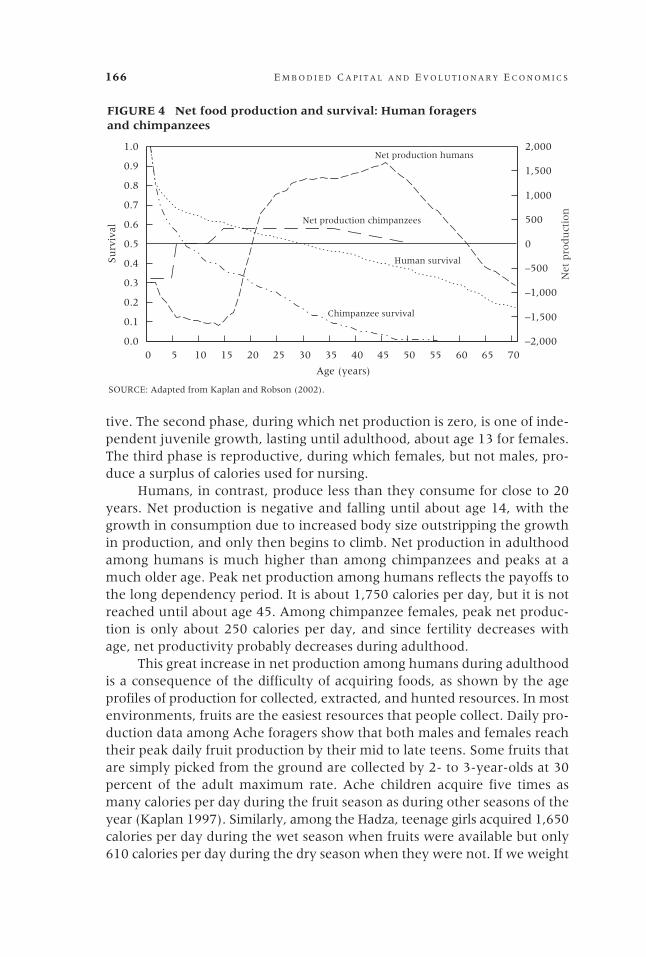
166 E M B O D I E D C A P I T A L A N D E V O L U T I O N A R Y E C O N O M I C S
tive. The second phase, during which net production is zero, is one of inde-pendent juvenile growth, lasting until adulthood, about age 13 for females.The third phase is reproductive, during which females, but not males, pro-duce a surplus of calories used for nursing.
Humans, in contrast, produce less than they consume for close to 20years. Net production is negative and falling until about age 14, with thegrowth in consumption due to increased body size outstripping the growthin production, and only then begins to climb. Net production in adulthoodamong humans is much higher than among chimpanzees and peaks at amuch older age. Peak net production among humans reflects the payoffs tothe long dependency period. It is about 1,750 calories per day, but it is notreached until about age 45. Among chimpanzee females, peak net produc-tion is only about 250 calories per day, and since fertility decreases withage, net productivity probably decreases during adulthood.
This great increase in net production among humans during adulthoodis a consequence of the difficulty of acquiring foods, as shown by the ageprofiles of production for collected, extracted, and hunted resources. In mostenvironments, fruits are the easiest resources that people collect. Daily pro-duction data among Ache foragers show that both males and females reachtheir peak daily fruit production by their mid to late teens. Some fruits thatare simply picked from the ground are collected by 2- to 3-year-olds at 30percent of the adult maximum rate. Ache children acquire five times asmany calories per day during the fruit season as during other seasons of theyear (Kaplan 1997). Similarly, among the Hadza, teenage girls acquired 1,650calories per day during the wet season when fruits were available but only610 calories per day during the dry season when they were not. If we weight
0 5 10 15 20 25 30 35 40 45 50 55 60 65 700.0
0.1
0.2
0.3
0.4
0.5
0.6
0.7
0.8
0.9
1.0
–2,000
–1,500
–1,000
–500
0
500
1,000
1,500
2,000
Su
rviv
al
Net
pro
du
ctio
n
Age (years)
FIGURE 4 Net food production and survival: Human foragers and chimpanzees
Human survival
Net production humans
Net production chimpanzees
Chimpanzee survival
SOURCE: Adapted from Kaplan and Robson (2002).
PDR 29 Supp Kaplan.sp 7/6/06, 3:22 PM166

H I L L A R D K A P L A N / J A N E L A N C A S T E R / A R T H U R R O B S O N 167
the wet and dry season data equally, Hadza teenage girls acquire 53 percentof their calories from fruits, compared to 37 percent and 19 percent for re-productive-aged and post-reproductive women (Hawkes, O’Connell, andBlurton Jones 1989).
In contrast, the acquisition rate of extracted resources often increasesthrough early adulthood as foragers acquire the necessary skills. Data onHiwi women show that root acquisition rates do not peak until about ages35 to 45 (Kaplan et al. 2000), and the rate for 10-year-old girls is only 15percent of the adult maximum. Hadza women appear to attain maximumroot digging rates by early adulthood (Hawkes, O’Connell, and Blurton Jones1989). Hiwi honey extraction rates by males peak at about age 25. Againthe extraction rate of 10-year-olds is less than 10 percent of the adult maxi-mum. Experiments among Ache women and girls clearly show that youngadult girls are not capable of extracting palm products at the rate attainedby older women (Kaplan et al. 2000). Ache women do not reach peak re-turn rates until their early 20s. !Kung (Ju/’hoansi) children crack mongongonuts at a much slower rate than adults (Blurton Jones, Hawkes, and Draper1994b), and nut cracking rates among the neighboring Hambukushu donot peak until about age 35 (Bock 1995). Finally, even chimpanzee juve-niles focus on more easily acquired resources than adult chimpanzees. Dif-ficult-to-extract resources such as termites and ants and activities such asnut cracking are practiced less by chimpanzee juveniles than adults (Boeschand Boesch 1999; Hiraiwa-Hasegawa 1990; Silk 1978).
The skill-intensive nature of human hunting and the long learningprocess involved are demonstrated by data on hunting return rates by age(see Kaplan et al. 2001 for details on why hunting is so cognitively demand-ing). Hunting return rates among the Hiwi do not peak until ages 30 to 35,with the acquisition rate of 10-year-old and 20-year-old boys reaching only16 percent and 50 percent of the adult maximum. The hourly return ratefor Ache men peaks in the mid-30s. The return rate of 10-year-old boys is amere 1 percent of the adult maximum, and the return rate of 20-year-oldjuvenile males is still only 25 percent of the adult maximum. Marlowe (un-published data, personal communication) obtains similar results for theHadza. Also, boys switch from easier tasks, such as fruit collection, shallowtuber extraction, and baobab processing, to honey extraction and huntingin their mid to late teens among the Hadza, Ache, and Hiwi (Blurton Jones,Hawkes, and O’Connell 1989, 1997; Kaplan et al. 2000). Even among chim-panzees, hunting is strictly an adult or near-adult activity (Boesch and Boesch1999; Stanford 1998; Teleki 1973).
A complex web of intrafamilial and interfamilial food flows and otherservices supports this age profile of energy production. First, there is thesexual division of labor. Men and women specialize in different kinds ofskill acquisition and then share the fruits of their labor. The specializationgenerates two forms of complementarity. Hunted foods acquired by men
PDR 29 Supp Kaplan.sp 7/6/06, 3:22 PM167

168 E M B O D I E D C A P I T A L A N D E V O L U T I O N A R Y E C O N O M I C S
complement gathered foods acquired by women, because protein, fat, andcarbohydrates complement one another with respect to their nutritionalfunctions (Hill 1988). The fact that male specialization in hunting produceshigh delivery rates of large, shareable packages of food leads to anotherform of complementarity. The meat inputs of men shift the optimal mix ofactivities for women, increasing time spent in childcare and decreasing timespent in food acquisition (Hurtado et al. 1992). They also shift women’stime to foraging and productive activities that are compatible with childcareand away from dangerous ones. In the ten-group sample, men, on average,acquired about twice as many calories and seven times as much protein aswomen (68 percent vs. 32 percent of the calories and 88 percent vs. 12percent of the protein) (Kaplan et al. 2000). We estimate that on average31 percent, 39 percent, and 30 percent of those calories support adult fe-male, adult male, and offspring consumption (Kaplan et al. 2001). This im-plies that after taking into account own consumption, women supply only3 percent of the calories to offspring and men provide the remaining 97percent. Men supply not only all of the protein and fat to offspring, but alsothe bulk of the protein and fat consumed by women. This contrasts sharplywith most (>97 percent) mammalian species, among which the female sup-ports all of the energetic needs of an offspring until it begins eating solidfoods (Clutton-Brock 1991) and males provide little or no investment. Thehigh productivity of men has probably allowed for the evolution of physi-ological adaptations among women, such as fat storage at puberty and againduring pregnancy—adaptations not found in apes.
Mortality
Figure 5 shows the mortality rates of chimpanzees (synthesized from fivechimpanzee sites; Hill et al. 2001) and two foraging groups (Ache: Hill andHurtado 1996: Table 6.1; Hadza: Blurton Jones et al. 2002: Table 2). Althoughthere are differences among chimpanzee and human foraging populations,the contrast between the two species is clear. Before the age of 5, mortalityrates are not very different between human foragers and chimpanzees. Theaverage mortality rate during the adult period differs greatly between thetwo species, as does the age at which mortality rates rise steeply. Mortalitywithin the two foraging groups remains quite low from adolescence to ages35 to 40 and rises abruptly after about age 65. Among chimpanzees, mortal-ity rates begin to rise quickly after their lowest point prior to reproduction.
The low adult mortality rates among humans are necessary componentsof delayed production. Only about 30 percent of chimpanzees ever born reach20, the age when humans produce as much as they consume, and less than 5percent of chimpanzees reach 45, when human net production peaks. Therelationship between survival rates and age profiles of production is made
PDR 29 Supp Kaplan.sp 7/6/06, 3:22 PM168

H I L L A R D K A P L A N / J A N E L A N C A S T E R / A R T H U R R O B S O N 169
even clearer in Figure 6 (adapted from Kaplan and Robson 2002). This plotsnet expected cumulative productivity by age, multiplying the probability ofbeing alive at each age times the net productivity at that age and then sum-ming over all ages up to the present. The unbroken and dotted lines showcumulative productivity by age for chimpanzees and humans, respectively. Thelonger human training period is evident when the troughs in the human andchimpanzee curves are compared. The dashed line is a hypothetical cross of
0 5 10 15 20 25 30 35 40 45 50 55 60 65 70 750.00
0.05
0.10
0.15
0.20
0.25
0.30
Pro
port
ion
dyi
ng
Age (years)
Chimpanzee
Ache
Hadza
FIGURE 5 Age-specific mortality rates: Chimpanzees andhuman foragers
0 5 10 15 20 25 30 35 40 45 50 55 60 65 70 75–7
–6
–5
–4
–3
–2
–1
0
1
2
Net
cal
ori
es (
millio
ns)
Age (years)
FIGURE 6 Cumulative expected net caloric production by age:Humans and chimpanzees
Human production,chimpanzee survival
Chimpanzee production,chimpanzee survival
Human production,human survival
SOURCE: Adapted from Kaplan and Robson (2002).
PDR 29 Supp Kaplan.sp 7/6/06, 3:22 PM169

170 E M B O D I E D C A P I T A L A N D E V O L U T I O N A R Y E C O N O M I C S
human production profiles with chimpanzee survival rates. It shows that thehuman production profile would not be viable with chimpanzee survival rates,because expected lifetime net production would be negative.
Finally, although the mortality data for the Ache and the Hadza arebased on small sample sizes and thus subject to considerable sample error,there is some evidence that proportional rates of change in mortality arenot constant during the adult period. Figure 7 shows proportional rates ofchange in mortality. Mean yearly mortality rates were determined for thefollowing age classes (10–14, 15–19, 20–29, 30–39, 40–49, 50–59, 60–69,70–79) and then transformed into natural logarithms. Differences in thosevalues between an age class and the preceding one were divided by thenumber of years in the age class to determine an average yearly rate ofincrease or decrease. For example, the first set of bars compares mortalityrates of 10–14-year-olds with those of 15–19-year-olds and shows that ratesdecreased by 1 percent per year and 6 percent per year among the Acheand Hadza, respectively. For the Ache, the data show virtually no change inmortality rates from age 10 to age 39. From age 40 to age 69, rates of in-crease vary between 2 and 6 percent per year, with the lowest rate of in-crease occurring during the 60s. However, mortality rates show a steep riseto about 14 percent per year after age 70. For the Hadza, mortality ratesactually decrease during the teens and 20s and stay essentially the sameduring the 30s. From age 40 to age 69, rates of increase vary between 0 and9 percent per year, also with the lowest rate of increase during the 60s.Again, mortality rates show a steep rise to about 12 percent per year afterage 70.
10–14 vs.15–19
15–19 vs.20–29
20–29 vs.30–39
30–39 vs.40–49
40–49 vs.50–59
50–59 vs.60–69
60–69 vs.70–79
–0.08
–0.06
–0.04
–0.02
0.00
0.02
0.04
0.06
0.08
0.10
0.12
0.14
0.16
An
nu
al p
erce
nt
chan
ge
Age (years)
Ache
Hadza
FIGURE 7 Yearly proportional change in mortality rates
PDR 29 Supp Kaplan.sp 7/6/06, 3:22 PM170

H I L L A R D K A P L A N / J A N E L A N C A S T E R / A R T H U R R O B S O N 171
The relative constancy of mortality rates during prime adulthood isstriking in both the Ache and the Hadza, as is the steep increase during the70s. This suggests that “rectangularization” of the mortality profile amonghumans (Fries 1980, 1989) predates modernization. It may be a fundamen-tal feature of our species, reflecting both strict genetic quality control be-fore implantation of the fetus (as discussed in detail by Ellison 2001) andincreased effort at slowing the rate of senescence during adulthood. Figure8 shows the adult mortality density function, conditional on surviving toage 15, for the Ache and Hadza (averaging the two groups and then smooth-ing with a five-year running average). Although samples are small at olderages, there is an apparent mode at 73 years of age. The pattern also mightsuggest that a good candidate for the natural human life span is about 65 to75 years, defined in terms of the imminence of death. This corresponds wellwith our impressions regarding physical deterioration. While some individu-als show marked decline in their late 50s to early 60s, others remain vigor-ous to age 70 or so. After this physical decline, death often follows within afew years. Unfortunately, however, very little is known about the timingand population distribution of physical decline among hunter-gatherers orother traditional subsistence-level peoples.
The life span
The human life course and human life span
Our fundamental thesis in this chapter is that the human life course is anintegrated adaptation to a specialized niche. Digestive physiology andanatomy; nutritional biochemistry; brain growth and cognitive development;tempo of body mass increases and appetite; age profiles of productivity, re-production, parental investment, and mortality; and, ultimately, the life span
15 20 25 30 35 40 45 50 55 60 65 70 750.000
0.005
0.010
0.015
0.020
0.025
0.030
0.035
Den
sity
Age (years)
FIGURE 8 Adult mortality density
PDR 29 Supp Kaplan.sp 7/6/06, 3:22 PM171

172 E M B O D I E D C A P I T A L A N D E V O L U T I O N A R Y E C O N O M I C S
are coadapted to a learning-intensive feeding niche, giving humans accessto the most nutrient-dense and highest-quality food resources. The jointexamination of these domains suggests a highly structured life course, inwhich six distinct stages can be recognized.
Brain growth occurs from the early fetal stage to about 5 years of age,with 90 percent occurring by age 3.0 to 3.5. Human mothers and their ba-bies maintain large fat reserves to support this brain growth (Ellison 2001;Kuzawa 1998). While cognitive development unfolds over many more years,a great deal of linguistic competence, especially comprehension, is achievedduring this first stage of life. Thus, it would seem that the human special-ization evident in the first stage of life is building the “physical plant” (i.e.,the brain) and the knowledge acquisition pathway (i.e., language ability)to support a long period of learning.
The second stage, childhood, is characterized by very slow physicalgrowth, a large energetic allocation to building the immune system (McDadeand Worthman 1999; Worthman 1999a), several important phases of cog-nitive development facilitated by play and other forms of practice, very lowproductivity, and very low mortality. Parents insist that children remain insafe places and encourage them to produce food only when it is easily andsafely acquired (Blurton Jones, Hawkes, and Draper 1994a). The uniquefeature of human childhood is that it is fully supported by familial energyinputs, reducing exposure to mortality hazards and allowing time for learn-ing. Faster physical growth would only make children more expensive be-fore their brains were ready for food production.
Adolescence follows, during which physical growth is accomplishedrapidly, the reproductive system matures, and the final phases of cogni-tive development occur. It is during this phase that the brain and the restof the body become ready for adult productivity. While productivity in-creases during adolescence, it is also largely supported by familial foodinputs.
For males, “on-the-job training” characterizes the period from earlyadulthood to prime adulthood in the mid to late 30s. Both physical strengthand information-processing speed (fluid intelligence) peak in early adult-hood, but knowledge-based abilities (crystallized intelligence) continue torise (Horn 1968). As a result, productivity increases many-fold during thisperiod. Mortality rates remain virtually constant and low. Resource pro-duction at this stage in the life course of women is very different. It is char-acterized by a reduction in productivity in the interests of fertility and pa-rental investment. Women face a tradeoff between resource acquisition andchildcare because the burden of children reduces foraging efficiency andbecause foraging often exposes children to environmental hazards. As a re-sult, women reduce their work or shift their activities toward food process-ing and other, less dangerous, efforts.
PDR 29 Supp Kaplan.sp 7/6/06, 3:22 PM172

H I L L A R D K A P L A N / J A N E L A N C A S T E R / A R T H U R R O B S O N 173
Middle age is a period of simultaneous parenthood and grandparent-hood. Dependency loads on parents peak around age 40, just before grand-parenthood begins. Although productivity is also at a peak level, net pro-ductivity including dependency loads is negative, supported by resourcetransfers from other families. Through middle age, dependency loads di-minish, as does productivity.
Old age commences around age 60, and during this seventh decade oflife physical deterioration proceeds rapidly and brain aging becomes evident,followed by a sharp increase in mortality rates. Parenting is finished and workeffort decreases along with productivity. This is not to say that there are nopositive contributions to fitness during this phase. Older adults attempt to beas productive as possible, reallocating their time to skill-intensive but less en-ergy-intensive activities (e.g., craft production and childcare; Gurven andKaplan 2001). They may also affect the productivity of the younger popula-tion through their knowledge of the habitat and through their political skills.
If this set of stages characterized the average life course of the last100,000 to 200,000 years, it is likely that the processes of maintenance andrepair from the intracellular level to the whole-organism level were shapedby selection to achieve a life span including all six stages. One possibility isthat the sixth stage is actually an artifact of selection intended to maintainthe body and mind in good condition through the first five stages of life.The sixth stage would then be the result of the impossibility of nature’sdesigning a body that collapses the moment high functionality is no longerneeded. Another possibility is that this sixth stage has been positively se-lected because of the fitness benefits produced during it.
Some (e.g., Hawkes et al. 1998; Williams 1957) have hypothesized thatthe benefits provided by grandmothers to grandchildren have selected formenopause and the long human life span. The data on child dependencyburdens suggest an alternative hypothesis: the life span is the result of se-lection on adults, allowing them to support all of their children throughadolescence, and this requires high productivity to about age 60 (Lancasterand King 1985; see Peccei 2001 for a recent statement and review). Thepost-reproductive period might then not begin until children are fully reared.Grandchildren are only half as related to grandparents as children are toparents. Therefore, at the margin, the benefits to grandchildren would haveto be twice as great as those to children to favor the same investment incontinued life.
This hypothesis of course depends upon menopause, which must beexplained as well. It is still unclear whether menopause is the result oftradeoffs between egg quality and reproductive life span, tradeoffs betweensupporting multiple dependent young and production of additional offspring,tradeoffs between grandparental investment and reproduction, or somethingelse (see Kaplan 1997 for a discussion).
PDR 29 Supp Kaplan.sp 7/6/06, 3:22 PM173

174 E M B O D I E D C A P I T A L A N D E V O L U T I O N A R Y E C O N O M I C S
Flexibility and variation in the human life span
The human brain is the physical medium through which culture is main-tained and transmitted. As such, it is generally thought to have greatly ex-panded the behavioral flexibility of our species relative to other animals. How-ever, the commitment to building and programming the brain requires a highlystructured life history that places constraints on the timing of life events. Ourspecies is committed to long-term neural and cognitive capital accrual and toa long life span. The characteristic life history of our ancestors has shaped ageprofiles of growth, tissue repair, and physical decline.
Nevertheless, human life histories show evidence of systematic varia-tion in response to environmental variation. Those effects appear to be theresult of the interaction between changes in environmental conditions andhuman physiology and behavior. Perhaps the most striking example of thatinteraction is the pattern of changes accompanying the secular trend to-ward modernization. Increased nutrition and decreased work and diseaseloads have systematic effects on human developmental physiology. Physi-cal growth rates have increased and maturation now begins earlier, result-ing in greater stature, higher body weight, and earlier age of menarche ingirls (Eveleth 1986; Lancaster 1986; Worthman 1999b). This response isvery likely the result of adaptive flexibility in growth and maturation in theface of variation in food supply and in disease assault rates that was experi-enced during human evolutionary history.
In contrast to this increase in the rate of physical development, agingmay be slowed in response to better nutrition and decreased work and dis-ease loads. Although it is possible that humans would also show slowedaging in response to radical reductions in caloric intake (as do rats in feed-ing experiments—see Shanley and Kirkwood 2000 for a review), it is alsopossible that within the usual range of variation, rates of aging are slowedand life spans are lengthened when nutrition is better and disease loads arelower (Fogel and Costa 1997). This outcome would also be adaptive. Thechanging mortality rates among older people accompanying modernizationand the fact that some chronic diseases occurred at earlier ages in the nine-teenth-century United States than today (Costa 2000) are consistent withthis possibility.
On the other hand, increased risk of heart disease, diabetes, and can-cer from overweight and lack of exercise may also be the result of evolvedresponses. Given the common activity regimes in our past and the variabil-ity in food supply, human appetites and nutritional biochemistry may bedesigned to store fat and increase blood lipid levels when food is abundant.Those adaptations might reduce the life span in the context of modern pat-terns of activity levels and food access and consumption.
In addition to these physiological adaptations, there are also behav-ioral responses to modernization. The models outlined in our first section
PDR 29 Supp Kaplan.sp 7/6/06, 3:22 PM174

H I L L A R D K A P L A N / J A N E L A N C A S T E R / A R T H U R R O B S O N 175
above are as applicable to short-term behavioral variation as they are tolong-term life-history adaptations. Two noteworthy effects of moderniza-tion are increased economic payoffs to educational capital and decreasedmortality owing to improvements in public health. The present models pre-dict reinforcing endogenous behavioral responses to such changes. Increasedpayoffs to education should promote increased investment both in educa-tional capital and in staying alive. Improvements in public health shouldalso promote reinforcing increases in capital investment and staying alive.It is an open question whether we are reaching the upper limit of our flex-ibility in the life span. It appears that with respect to stature and perhapsage of menarche, we have reached the limit. There appears to be more scopefor variation in the life span, given investments in medical technology de-signed to reduce disease and the effects of aging. In any case, knowledgeabout the human genome is likely to lead to manipulations of genes andgene products, resulting in life span increases of very large magnitude.
Building blocks for an adequate theory of senescenceand the life span
Given the definition of life span guiding this discussion (the span from birthto the age when death is imminent as a result of physical deterioration), anadequate theory of life span will require a theory of senescence. Each of theprincipal theories suffers from important weaknesses, rendering the theoryincomplete. This section first reviews those weaknesses and then offers aframework intended to remedy them.
Senescence is generally defined as an increasing mortality rate withage. The theories proposed by Medawar (1952), Williams (1957), andHamilton (1966) share the common premise that senescence is the mani-festation of the decreasing force of selection with age, resulting from ex-trinsically imposed hazards of mortality. In essence, their argument is thatsources of mortality that strike when the individual is old are less strin-gently selected against than those striking when young, simply because anindividual has a greater probability of being young than old.
According to Williams (1957), antagonistic pleiotropy accounts for theincrease in mortality with age. Senescence is due to the presence of geneswith opposing pleiotropic effects at different ages, increasing survival atyounger ages but decreasing survival at older ages or increasing fertility atyounger ages at the expense of reduced survival at older ages. Since extrin-sically imposed mortality decreases the force of selection with age, geneswith such positive effects at younger ages and negative effects at older ageswill accumulate through selection, producing increasing mortality rates withage. He speculated that selection on mortality at each age would vary withreproductive value (i.e., expected future reproduction conditional on beingalive at that age). Hamilton (1966) formalized this argument and showed
PDR 29 Supp Kaplan.sp 7/6/06, 3:22 PM175

176 E M B O D I E D C A P I T A L A N D E V O L U T I O N A R Y E C O N O M I C S
that sensitivities of fitness to changes in mortality rates decrease with theage of action. However, his results suggested that reproductive value is notthe critical determinant, because the sensitivity of fitness to changes in mor-tality rates depends both on the probability of reaching that age and onexpected future reproduction at that age.
According to the formal model discussed above, the fact that mortalitydiscounts the future does not, in itself, select for increasing mortality rateswith age. Our approach allows both capital investments and expenditure onmortality reduction to be subject to natural selection. If aging, in the sense ofexplicit time dependence, is not built-in, then positive but constant mortalityrates and a constant capital stock are optimal. This is so because our modelassumes that current mortality can be reduced by current energy expendi-ture. From an initial viewpoint, reducing future mortality is indeed less im-portant than reducing present mortality, just because survival is not certain.However, future expenditures on mortality reduction should be discountedfor the same reason, and in the long run these two effects are precisely offset-ting. If mortality is avoided during a time interval, the organism faces thesame tradeoff between reproduction and survival as earlier.
This result does not depend on the assumption that current mortalityis reduced by current expenditures. An alternative model might assume theexistence of a stock of somatic capital for determining mortality, as seems aplausible explicit interpretation of Kirkwood’s (1990) “disposable somatheory.” However, it can be shown that the optimal life history may againentail a steady state in which this stock, and hence the mortality rate, areconstant. From a current viewpoint, the tradeoff between the present andthe future, as reflected in the decision about the size of the stock, is station-ary. Even when decisions are made at the beginning of life, both the costsand benefits of future mortality control are deflated in the same way. Fi-nally, even if somatic capital depreciates over time, results from capital in-vestment theory show that the stock will be maintained at an optimal level(Arrow and Kurz 1970; Intriligator 1971). Optimal investment in the capi-tal stock will continue to precisely offset depreciation. As long as produc-tion is constant with a constant capital stock, optimal mortality rates re-main constant as well.4
What then causes senescence? Suppose there are cost functions forbuilding embodied capital and for repairing and maintaining embodied capi-tal. Imagine that the embodied capital stock is described in terms of twostate variables, the quantity of the stock and its efficiency. From its incep-tion, the organism builds somatic capital, adding to its quantity until theoptimal quantity is reached. However, because of its own metabolic activityand assaults from outside agents, the efficiency of the capital stock is sub-ject to decay. For example, free radicals and other harmful molecules mayaccumulate in cells, accidents may cause tissue damage, and pathogens may
PDR 29 Supp Kaplan.sp 7/6/06, 3:22 PM176

H I L L A R D K A P L A N / J A N E L A N C A S T E R / A R T H U R R O B S O N 177
disrupt physiological function and damage cells. In the same sense that thecosts of producing new car seats may be different from the costs of repair-ing tears in those seats, the costs of producing new cells and adding to thequantity of embodied capital may be different from the costs of repairingdamage to them. Thus, during development, the optimal life-history pro-gram will have to equalize marginal fitness returns from three different in-vestments: adding to new capital, repairing existing capital, and reducingcurrent mortality. When the capital stock reaches the level at which someallocation to reproduction is also optimal, marginal returns from investmentsin producing new capital in the form of descendants must also be equalizedwith the marginal returns from the other three investments.
It is possible that for many capital stocks, quantity increases with agewhile efficiency decreases because, as suggested by Kirkwood (1990), opti-mal repair is not complete. Such a process appears to characterize cognitivedevelopment and aging. For example, verbal knowledge tends to increase,at least through middle age, but information-processing speed and memorypeak during the third decade and decline thereafter (Schaie 1996). Duringthe first phase of life, those increases in quantity have larger effects on thevalue of life (i.e., the expected future contribution to fitness) than do thedecreases in efficiency. Thus productivity increases and optimal mortalitydecreases. However, at some age, the effects of disrepair overwhelm theeffects of growth and learning, and overall productivity and the ability tofend off mortality hazards are lessened. This would lead to increasing opti-mal mortality with age.
This framework, with four kinds of investment, may provide a moreadequate basis for a general theory of life-history evolution, and of life spanin particular. Without making the unrealistic assumption that any life-his-tory component, such as mortality, is extrinsic, selection can act to opti-mize and coadapt each of those components. Given the results discussedabove, it is plausible that exogenous factors increasing the productivity ofcapital should select not only for increased capital investments and reducedmortality rates, but also for higher optimal allocations to repair, because ofthe higher probability of reaching old age. This would then lead to a longerlife span. Similarly, exogenous factors that affect mortality rates may selectnot only for greater capital investment and reinforcing increases in optimalallocations to reducing mortality rates, but also for slower senescence. Givenniche differentiation in the payoffs to body size and learning, in the payoffsto investment in offspring, in the payoffs to reducing mortality rates, andpossibly in the payoffs to repair, the wide array of life histories found innature is not surprising.
Whether such a framework will be useful awaits the formal develop-ment of models designed to analyze the effects of selection on those invest-ment functions. It does, however, direct empirical attention to measuring
PDR 29 Supp Kaplan.sp 7/6/06, 3:22 PM177

178 E M B O D I E D C A P I T A L A N D E V O L U T I O N A R Y E C O N O M I C S
the shapes of those functions. What are the costs and benefits of reducingthe quantities of harmful molecules in cells, of DNA repair, and of differingnumbers and kinds of immune cells? How do those costs and benefits com-pare to those associated with increases in muscle mass, brain mass, and learn-ing? And, how do each of those functional relationships compare with thosecharacterizing the production of offspring of different sizes and differentfunctional abilities? Regardless of the ultimate productivity of this evolu-tionary economic life-history framework, understanding those relationshipsis likely to be illuminating.
Notes
This chapter was written with support from theNational Institute on Aging, grant numberAG15906. The authors acknowledge the con-tributions of Kim Hill to the data sets and theiranalyses on the comparative diets and demog-raphy of chimpanzees and foragers publishedpreviously (Kaplan et al. 2000). We also thankKim Hill and Magdalena Hurtado for their dataon resource acquisition by age and sex amongthe Hiwi and Ache (Kaplan et al. 2000). Thesedata sets and analyses form a critical base forthe second part of this chapter.
1 Of course, a quantitative definitionwould require specification of that ratio.
2 In some cases, there may be some addi-
tional mortality increases and drops due tophase transitions such as weaning.
3 The fourth subperiod, covering abilitiessuch as recognition of conservation of quanti-ties of liquids under container transformations,seems to require tutelage and symbolic training.
4 Medawar’s (1952) model, in which del-eterious mutations with age-specific effects latein life accumulate owing to the weaker forceof selection at older ages, does not suffer fromthis problem. However, it can only account forspecific diseases with late onset, not for thegeneral and progressive deterioration of thesoma with age, nor the physiological processesunderlying aging.
References
Aiello, L. and P. Wheeler. 1995. “The expensive-tissue hypothesis: The brain and the diges-tive system in human and primate evolution,” Current Anthropology 36: 199–221.
Allman, J., T. McLaughlin, and A. Hakeem. 1993. “Brain weight and life-span in primatespecies,” Proceedings of the National Academy of Sciences 90: 118–122.
Armstrong, E. and D. Falk (eds.). 1982. Primate Brain Evolution. New York: Plenum Press.Arrow, K. J. and M. Kurz. 1970. Public Investment, the Rate of Return, and Optimal Fiscal Policy.
Baltimore, MD: Johns Hopkins Press.Becker, G. S. 1975. Human Capital. New York: Columbia University Press.Blurton Jones, N. G. 2002. “Antiquity of postreproductive life: Are there modern impacts
on hunter-gatherer postreproductive life spans?” American Journal of Human Biology14: 184–205.
Blurton Jones, N. G., K. Hawkes, and P. Draper. 1994a. “Differences between Hadza and!Kung children’s work: Original affluence or practical reason?,” in E. S. Burch and L.Ellana (eds.), Key Issues in Hunter Gatherer Research. Oxford: Berg, pp. 189–215.
———. 1994b. “Foraging returns of !Kung adults and children: Why didn’t !Kung childrenforage?,” Journal of Anthropological Research 50: 217–248.
Blurton Jones, N., K. Hawkes, and J. O’Connell. 1989. “Modeling and measuring the costsof children in two foraging societies,” in V. Standen and R. A. Foley (eds.), Compara-tive Socioecology of Humans and Other Mammals. London: Basil Blackwell, pp. 367–390.
PDR 29 Supp Kaplan.sp 7/6/06, 3:22 PM178

H I L L A R D K A P L A N / J A N E L A N C A S T E R / A R T H U R R O B S O N 179
———. 1997. “Why do Hadza children forage?,” in N. L. Segal, G. E. Weisfeld, and C. C.Weisfield (eds.), Uniting Psychology and Biology: Integrative Perspectives on Human Develop-ment. New York: American Psychological Association, pp. 297–331.
Bock, J. A. 1995. “The determinants of variation in children’s activities in a southern Afri-can community,” unpublished Ph.D. dissertation, Department of Anthropology Uni-versity of New Mexico, Albuquerque.
Boesch, C. and H. Boesch. 1999. The Chimpanzees of the Tai Forest: Behavioural Ecology andEvolution. Oxford: Oxford University Press.
Bunn, H. T. 2001. “Hunting, power scavenging, and butchering among Hadza foragers andPlio-Pleistocene Homo,” in C. B. Stanford and H. T. Bunn (eds.), Meat-eating and Hu-man Evolution. Oxford: Oxford University Press, pp. 199–218.
Carey, J. R. and D. S. Judge. 2001. “Life span extension in humans is self-reinforcing: Ageneral theory of longevity,” Population and Development Review 27: 411–436.
Charnov, E. L. 1993. Life History Invariants: Some Explanations of Symmetry in Evolutionary Ecol-ogy. Oxford: Oxford University Press.
Clutton-Brock, T. H. 1991. The Evolution of Parental Care. Princeton: Princeton University Press.Cordain, L., J. Brand Miller, S. B. Eaton, N. Mann, S. H. A. Holt, and J. D. Speth. 2000.
“Plant-animal subsistence ratios and macronutrient energy estimations in hunter-gath-erer diets,” American Journal of Clinical Nutrition 71: 682–692.
Cordain, L., S. B. Eaton, J. Brand Miller, N. Mann, and K. Hill. 2002. “The paradoxicalnature of hunter-gatherer diets: Meat based, yet non-atherogenic,” European Journalof Clinical Nutrition 56(supp): 542–552.
Costa, D. L. 2000. “Understanding the twentieth century decline in chronic conditions amongolder men,” Demography 37: 53–72.
Deacon, T. 1997. The Symbolic Species. New York: W. W. Norton.Ellison, P. T. 2001. On Fertile Ground: A Natural History of Human Reproduction. Cambridge,
MA: Harvard University Press.Emken, R. A., R. O. Adlof, W. K. Rohwedder, and R. M. Gulley. 1992. “Comparison of
linollenic and linoleic acid metabolism in man: Influence of linoleic acid,” in A. Sinclairand R. Gibson (eds.), Essential Fatty Acids and Eicosanoids: Invited Papers from the ThirdInternational Conference. Champaign, IL: AOCS Press, pp. 23–25.
Eveleth, P. B. 1986. “Timing of menarche: Secular trend and population differences,” inJ. B. Lancaster and B. A. Hamburg (eds.), School-Age Pregnancy and Parenthood.Hawthorne, NY: Aldine de Gruyter, pp. 39–53.
Finch, C. E. 1998. “Variations in senescence and longevity include the possibility of negli-gible senescence,” Journal of Gerontology: Biological Sciences 53A: B235–B239.
———. 2002. “Evolution and the plasticity of aging in the reproductive schedules in long-lived animals: The importance of genetic variation in neuroendocrine mechanisms,”in D. Pfaff, A. Arnold, A. Etgen, S. Fahrback, and R. Rubin (eds.), Hormones, Brain andBehavior. San Diego: Academic Press.
Finch, C. E. and R. M. Sapolsky. 1999. “The evolution of Alzheimer disease, the reproduc-tive schedule and the apoE isoforms,” Neurobiology of Aging 20: 407–428.
Fleagle, J. G. 1999. Primate Adaptation and Evolution. New York: Academic Press.Fogel, R. W. and D. L. Costa. 1997. “A theory of technophysio evolution, with some impli-
cations for forecasting population, health care costs and pension costs,” Demography34: 49–66.
Fries, J. F. 1980. “Ageing, natural death and the compression of morbidity,” New EnglandJournal of Medicine 303: 130–136.
———. 1989. “The compression of morbidity: Near or far?,” Milbank Quarterly 67: 208–232.Gadgil, M. and W. H. Bossert. 1970. “Life historical consequences of natural selection,”
American Naturalist 104: 1–24.Gibson, K. R. 1986. “Cognition, brain size and the extraction of embedded food resources,”
in J. G. Else and P. C. Lee (eds.), Primate Ontogeny, Cognition, and Social Behavior. Cam-bridge: Cambridge University Press, pp. 93–105.
PDR 29 Supp Kaplan.sp 7/6/06, 3:22 PM179

180 E M B O D I E D C A P I T A L A N D E V O L U T I O N A R Y E C O N O M I C S
Gurven, M. and H. Kaplan. 2001. “Determinants of time allocation to production across thelifespan among the Machiguenga and Piro Indians of Peru,” Albuquerque, NM: De-partment of Anthropology, University of New Mexico.
Hakeem, A., G. R. Sandoval, M. Jones, and J. Allman. 1996. “Brain and life span in pri-mates,” in R. P. Abeles, M. Catz, and T. T. Salthouse (eds.), Handbook of the Psychologyof Aging. San Diego: Academic Press, pp. 78–104.
Hamilton, W. D. 1966. “The molding of senescence by natural selection,” Journal of Theo-retical Biology 12: 12–45.
Hawkes, K., J. F. O’Connell, and N. Blurton Jones. 1989. “Hardworking Hadza grandmoth-ers,” in V. Standen and R. A. Foley (eds.), Comparative Socioecology of Humans and OtherMammals. London: Basil Blackwell, pp. 341–366.
Hawkes, K., J. F. O’Connell, N. G. Blurton Jones, H. Alvarez, and E. L. Charnov. 1998.“Grandmothering, menopause, and the evolution of human life histories,” Proceedingsof the National Academy of Science 95: 1336–1339.
Hill, K. 1988. “Macronutrient modifications of optimal foraging theory: An approach usingindifference curves applied to some modern foragers,” Human Ecology 16: 157–197.
Hill, K., C. Boesch, J. Goodall, A. Pusey, J. Williams, and R. Wrangham. 2001. “Mortalityrates among wild chimpanzees,” Journal of Human Evolution 39: 1–14.
Hill, K. and A. M. Hurtado. 1996. Ache Life History: The Ecology and Demography of a ForagingPeople. Hawthorne, NY: Aldine.
Hill, K. and H. Kaplan. 1999. “Life history traits in humans: Theory and empirical studies,”Annual Review of Anthropology 28: 397–430.
Hiraiwa-Hasegawa, M. 1990. “The role of food sharing between mother and infant in theontogeny of feeding behavior,” in T. Nishida (ed.), The Chimpanzees of the Mahale Moun-tains: Sexual and Life History Strategies. Tokyo: Tokyo University Press, pp. 267–276.
Holliday, M. A. 1978. “Body composition and energy needs during growth,” in F. Falkerand J. M. Tanner (eds.), Human Growth. New York: Plenum Press, pp. 117–139.
Horn, J. L. 1968. “Organization of abilities and the development of intelligence,” Psychologi-cal Review 75: 242–259.
Hurtado, A. M. and K. Hill. 1990. “Seasonality in a foraging society: Variation in diet, workeffort, fertility, and the sexual division of labor among the Hiwi of Venezuela,” Jour-nal of Anthropological Research 46: 293–345.
Intriligator, M. D. 1971. Mathematical Optimization and Economic Theory. Englewood Cliffs,NJ: Prentice-Hall.
Jerison, H. J. 1973. Evolution of the Brain and Intelligence. New York: Academic Press.———. 1976. “Paleoneurology and the evolution of mind,” Scientific American 234: 90–101.Judge, D. S. and J. R. Carey. 2000. “Postreproductive life predicted by primate patterns,”
Journal of Gerontology: Biological Sciences 55A: B201–B209.Kaplan, H. S. 1997. “The evolution of the human life course,” in K. Wachter and C. Finch
(eds.), Between Zeus and the Salmon: The Biodemography of Longevity. Washington, DC:National Academy of Sciences, pp. 175–211.
Kaplan, H., M. Gurven, K. R. Hill, and A. M. Hurtado. In press. “The natural history ofhuman food sharing and cooperation: A review and a new multi-individual approachto the negotiation of norms,” in H. Gintis, S. Bowles, R. Boyd, and E. Fehr (eds.),Moral Sentiments: Theory, Evidence and Policy. Cambridge: Cambridge University Press.
Kaplan, H. S., K. Hill, A. M. Hurtado, and J. B. Lancaster. 2001. “The embodied capitaltheory of human evolution,” in P. T. Ellison (ed.), Reproductive Ecology and Human Evo-lution. Hawthorne, NY: Aldine de Gruyter.
Kaplan, H., K. Hill, J. B. Lancaster, and A. M. Hurtado. 2000. “A theory of human lifehistory evolution: Diet, intelligence, and longevity,” Evolutionary Anthropology 9: 156–185.
Kaplan, H. S. and A. Robson. 2002. “The emergence of humans: The coevolution of intelli-gence and longevity with intergenerational transfers,” Proceedings of the National Acad-emy of Sciences 99: 10221–10226.
PDR 29 Supp Kaplan.sp 7/6/06, 3:22 PM180

H I L L A R D K A P L A N / J A N E L A N C A S T E R / A R T H U R R O B S O N 181
Kirkwood, T. B. L. 1990. “The disposable soma theory of aging,” in D. E. Harrison (ed.),Genetic Effects on Aging II. Caldwell, NJ: Telford Press, pp. 9–19.
Kozlowski, J. and R. G. Wiegert. 1986. “Optimal allocation to growth and reproduction,”Theoretical Population Biology 29: 16–37.
Kuzawa, C. W. 1998. “Adipose tissue in human infancy and childhood: An evolutionaryperspective,” Yearbook of Physical Anthropology 41: 177–209.
Lack, D. 1968. Ecological Adaptations for Breeding in Birds. London: Methuen.Lancaster, J. B. 1986. “Human adolescence and reproduction: An evolutionary perspec-
tive,” in J. B. Lancaster and B. A. Hamburg (eds.), School-Age Pregnancy and Parenthood.Hawthorne, NY: Aldine de Gruyter, pp. 17–39.
Lancaster, J. B. and B. J. King. 1985. “An evolutionary perspective on menopause,” in V.Kerns and J. K. Brown (eds.), In Her Prime: A View of Middle Aged Women. Garden City,NJ: Bergen and Garvey, pp. 13–20.
Lee, R. B. 1979. The !Kung San: Men, Women, and Work in a Foraging Society. Cambridge: Cam-bridge University Press.
Lee, R. B. and I. DeVore (eds.). 1968. Man the Hunter. Chicago: Aldine.Leigh, S. R. and B. T. Shea. 1996. “Ontogeny of body size variation in African apes,” Ameri-
can Journal of Physical Anthropology 99: 43–65.Lessells, C. M. 1991. “The evolution of life histories,” in J. R. Krebs and N. B. Davies (eds.),
Behavioural Ecology. Oxford: Blackwell, pp. 32–65.McDade, T. W. and C. M. Worthman. 1999. “Evolutionary process and the ecology of hu-
man immune function,” American Journal of Human Biology 11: 705–717.Medawar, P. B. 1952. An Unsolved Problem in Biology. London: Lewis.Mincer, J. 1974. Schooling, Experience, and Earnings. Chicago: National Bureau of Economic
Research.Murdock, G. P. 1967. “Ethnographic atlas: A summary,” Ethnology 6: 109–236.Parker, S. T. and M. L. McKinney. 1999. Origins of Intelligence: The Evolution of Cognitive Devel-
opment in Monkeys, Apes and Humans. Baltimore: Johns Hopkins Press.Promislow, D. E. L. 1991. “Senescence in natural populations of mammals: A comparative
study,” Evolution 45: 1869–1887.Promislow, D. E. L. and P. H. Harvey. 1990. “Living fast and dying young: A comparative
analysis of life history variation among mammals,” Journal of Zoology 220: 417–437.Richards, M. P. and R. M. Hedges. 2000. “Focus: Gough’s Cave and Sun Hole Cave human
stable isotope values indicated a high animal protein diet in the British Upper Pale-olithic,” Journal of Archeological Science 27: 1–3.
Richards, M. P., P. B. Pettitt, E. Trinkaus, F. H. Smith, M. Paunovic, and I. Karavanic. 2000.“Neanderthal diet at Vindija and Neanderthal predation: The evidence from stableisotopes,” Proceedings of the National Academy of Sciences 97: 7663–7666.
Robson, A. and H. Kaplan. 2002. “The coevolution of intelligence and longevity in hunter-gatherer economies.” London, Ontario: Department of Economics, University of West-ern Ontario.
Roff, D. A. 1992. The Evolution of Life Histories. London: Chapman and Hall.Sacher, G. A. 1959. “Relation of lifespan to brain weight and body weight in mammals,” in
G. E. W. Wolstenhome and M. O’Connor (eds.), Ciba Foundation Colloquia on Ageing.London: Churchill, pp. 115–133.
Schaie, K. W. 1996. Intellectual Development in Adulthood: The Seattle Longitudinal Study. NewYork: Cambridge University Press.
Schoeninger, M., H. T. Bunn, S. Murray, T. Pickering, and J. Moore. 2001. “Meat-eating bythe fourth African ape,” in C. B. Stanford and H. T. Bunn (eds.), Meat-eating and Hu-man Evolution. Oxford: Oxford University Press, pp. 179–195.
Shanley, D. P. and T. B. L. Kirkwood. 2000. “Calorie restriction and aging: A life-historyanalysis,” Evolution 54: 740–750.
Sibly, R. M. 1991. “The life-history approach to physiological ecology,” Functional Ecology 5:184–191.
PDR 29 Supp Kaplan.sp 7/6/06, 3:22 PM181

182 E M B O D I E D C A P I T A L A N D E V O L U T I O N A R Y E C O N O M I C S
Sibly, R., P. Calow, and N. Nichols. 1985. “Are patterns of growth adaptive?,” Journal ofTheoretical Biology 112: 553–574.
Silk, J. B. 1978. “Patterns of food-sharing among mother and infant chimpanzees at GombeNational Park, Tanzania,” Folia Primatologica 29: 129–141.
Stanford, C. B. 1998. Chimpanzee and Red Colobus: The Ecology of Predator and Prey. Cambridge,MA: Harvard University Press.
Stearns, S. C. 1992. The Evolution of Life Histories. Oxford: Oxford University Press.Tatar, M., D. W. Grey, and J. R. Carey. 1997. “Altitudinal variation in senescence in a
Melanoplus grasshopper species complex,” Oecologia 111: 357–364.Teleki, G. 1973. The Predatory Behavior of Wild Chimpanzees. Lewisburg, PA: Bucknell Univer-
sity Press.Williams, G. C. 1957. “Pleiotropy, natural selection and the evolution of senescence,” Evo-
lution 11: 398–411.Worthman, C. M. 1999a. “Epidemiology of human development,” in C. Panter-Brick and
C. M. Worthman (eds.), Hormones, Health and Behavior: A Socioecological and LifespanPerspective. Cambridge, UK: Cambridge University Press, pp. 47–105
———. 1999b. “Evolutionary perspectives on the onset of puberty,” in W. R. Trevathan, E.O. Smith, and J. J. McKenna (eds.), Evolutionary Medicine. Oxford: Oxford UniversityPress, pp. 135–163.
PDR 29 Supp Kaplan.sp 7/6/06, 3:22 PM182

183
Rescaling the LifeCycle: Longevity andProportionality
RONALD LEE
JOSHUA R. GOLDSTEIN
Since 1900 life expectancy in the United States has increased by about 30years, from 48 to 77 years. Most projections foresee continued increase at aslower rate, reaching 85 or 90 years by 2100 (Lee and Carter 1992; Tuljapurkaret al. 2000). Some analysts foresee the possibility of far greater life expect-ancy increases—to 100, 150 years, or more (Manton et al. 1991; Ahlburgand Vaupel 1990; Schneider et al. 1990). Individuals welcome longer life,but for populations, increases of this magnitude could impose heavy costson the working-age groups and could have other substantial but uncertaineconomic and social consequences. These consequences will depend in largepart on how the additional expected years of life are distributed across thevarious social and economic stages of the life cycle. This chapter speculatesabout how the gains will be used and how the life cycle will be modified.
Proportional rescaling of the life cycle, in which every life cycle stageand boundary simply expands in proportion to increased life expectancy,provides a convenient benchmark. Under proportional rescaling, if longev-ity doubles, then so would childhood, the length of work and retirement,the span of childbearing, and all other stages of the life cycle. Proportionalrescaling of the life cycle would appear to be neutral in some sense, so thatlife, society, and economy could continue as before, except that there wouldbe proportionately more time spent in every stage. However, we will findthat while this is (or could be) true for some aspects of life, other aspectswould vary with the square or some other power of longevity.
Although proportional rescaling may seem natural, and indeed doesoccur in nature as we discuss, powerful forces impede its application to hu-mans. First are biological constraints related to human development, suchas menarche and menopause, even though our vigor and health may ad-vance with longevity. Second are institutional constraints, for example on
PDR 29 Supp Lee.sp 7/6/06, 3:23 PM183

184 R E S C A L I N G T H E L I F E C Y C L E
schooling and retirement. Although these may adjust in the long run, overshorter horizons they may block proportional rescaling. Third, stock-flowinconsistencies may cause human and physical capital to rise with longev-ity more rapidly than labor force size, causing wages and incomes to riseand the interest rate and returns to human capital to fall, triggering furtheradjustments. If time in retirement is a luxury, then it may rise rapidly asincomes rise, so that age at retirement does not rise in proportion to lon-gevity—as in fact it has not. For these and other reasons, we should notactually expect to observe proportional rescaling in connection with in-creased life span in the past, nor should we anticipate it for the future. None-theless, proportionality is a useful benchmark against which to comparepast changes and the hypothetical future.
What would proportional rescaling look like?
A perfectly proportional rescaling of the life cycle accompanying increasedlife expectancy would appear indistinguishable from the effect of a simplechange in the units of measurement of age/time, as if we had changed fromdollars to pesos or from inches to centimeters. For example, suppose that anoriginal 75-year life cycle were instead measured in units of six lunar months,or half-years. The new life cycle would be 150 units long instead of 75, butof course nothing would be different. (We use doubling as a convenient ex-ample, but we believe that a 15 percent increase in life cycle is more likelyfor the twenty-first century.) Every life cycle stage would last twice as longas before, measured in the new units. Every rate would be only half as great,since only half as many events would take place in 6 months as in 12 months.
Proportional life cycle changes can occur in both strong and weak forms.In the strongest form, the change affects not only the average timing of lifecycle transitions but also the whole distribution of timing within a popula-tion. Thus, for example, the spread around the mean age of death or meanage of childbirth would also double if the mean age of death doubled. Wecall this “strong proportionality,” which can apply both to the distributionof an event among the individuals in a population and to the timing orlevel of an event in the individual life cycle. If the change in life cycle tim-ing is only proportional with respect to the mean ages of each life cycletransition or stage, then we call this “weak proportionality.” Weak propor-tionality would occur if, for example, as longevity increased, the mean ageof reproduction increased proportionately but the variance of the net ma-ternity function stayed constant.
It is important to distinguish between “flow” or “rate” variables, whichare measured per unit of time, and “stock” variables, which are not. Com-pleted fertility, accumulated wealth, the probability of ever marrying, or ofever having a first birth, are all examples of stocks. Birth rates, death rates,
PDR 29 Supp Lee.sp 7/6/06, 3:23 PM184

R O N A L D L E E / J O S H U A R . G O L D S T E I N 185
wage rates, income, and rate of knowledge acquisition are flows, all mea-sured per unit of time. Under the perfectly proportional rescaling of the lifecycle discussed above, all stocks are unchanged, provided they are assessedat the same proportional stage of the life cycle (for example at the age equalto 60 percent of life expectancy). In a population with a life expectancytwice as great, the net reproduction rate (NRR) would not be twice as high;it would be unchanged. All flow or rate variables, however, would be re-duced in inverse proportion to the increase in longevity. Adding these re-duced rates across twice as long an age span of reproduction would thenyield an unchanged completed fertility.1 We might say that perfectly pro-portional rescaling of the life cycle is always “stock constrained,” in the sensethat the magnitude of stocks is preserved under rescaling.
In some cases, this kind of stock-constrained rescaling is not an inter-esting scenario to contemplate. For example, if people were to live twice aslong, we would not expect that at each age they would earn only half asmuch, or that they would learn only half as much during each year in school.In these cases, it is more natural to assume that the rate of productivity, orearning, or acquisition of knowledge, remains constant, so that the stock oflifetime earnings, or completed education, would double. Such cases wecall “flow constrained.”
Figure 1 illustrates some hypothetical examples of what proportionalrescaling would look like under different assumptions, all of which assumethe convenient, yet implausible doubling of longevity. The top row illus-trates strong proportionality with stock constraints, such as might be thecase with fertility. Here the ages at which flows occur are doubled, but atthe same time the flow itself is halved. The result is that lifetime completedfertility remains unchanged, although the age at which a given cumulativefertility is achieved is doubled. The middle row shows strong proportional-ity with flow constraints, such as might be the case with earnings. The ageat which a given flow occurs in the rescaled age profile is twice that of theoriginal profile. Keeping flows constant over a longer period of time, how-ever, produces a doubling of the stock, for example cumulative lifetime earn-ings (and perhaps derived stocks, such as lifetime savings, which we discusslater). The bottom row illustrates a particular case of weak proportionality.Here the mean age of the flow doubles from 25 to 50, but the width of theage profile does not expand proportionally.
Proportional rescaling in nature
The object of this chapter is to explore the feasibility of proportional rescalingwithin a single species, namely humans. A large body of work already existslooking at proportional rescaling between biological species. In biology thisfalls under the study of “biological invariants” (Charnov 1993). Figure 2 shows
PDR 29 Supp Lee.sp 7/6/06, 3:23 PM185

FIGURE 1 Illustrative examples of proportional rescaling under ahypothetical doubling of longevity
Flows
0.00
0.02
0.04
0.06
0.08
0 20 40 60 80 100
Rat
e per
yea
rFlow-constrained strong proportionality
0.00
0.02
0.04
0.06
0.08
0 20 40 60 80 100
Rat
e per
yea
r
Age (years)
Weak proportionality
Stocks
0.0
0.5
1.0
1.5
2.0
0 20 40 60 80 100
Sto
ck a
t ag
e x
0.0
0.5
1.0
1.5
2.0
0 20 40 60 80 100
Sto
ck a
t ag
e x
Age (years)
NOTES: Original age profile is shown as a solid line, rescaled profile as dashed line. Stocks at age x arethe integral of flows from age zero to x. In this figure, flow-constrained strong proportionality isobtained by doubling ages at which a given rate is originally observed, resulting in a doubling ofeventual stocks; stock-constrained strong proportionality is obtained by simultaneously doubling agesand halving flows; and weak proportionality is obtained by doubling the mean of the flows whilekeeping the standard deviation of flows unchanged.
0.00
0.02
0.04
0.06
0.08
0 20 40 60 80 100
Rat
e per
yea
r
Stock-constrained strong proportionality
0.0
0.5
1.0
1.5
2.0
0 20 40 60 80 100
Sto
ck a
t ag
e x
PDR 29 Supp Lee.sp 7/6/06, 3:23 PM186

R O N A L D L E E / J O S H U A R . G O L D S T E I N 187
an example of such an invariant across mammalian species: the relationshipbetween age at physical maturity (m) and expected years of adulthood e(m).Goldstein and Schlag (1999) show a similar figure for the relationship be-tween mean age of reproduction and life expectancy at birth. Other examplesof biological invariants include the ratio of body mass to life expectancy atbirth; the product of the number of offspring and the chance of survival tothe mean age of reproduction; and metabolic invariants (Austad 1997). “In-variant” is used by biologists not as a rule to which there are no exceptionsbut rather to describe general tendencies, with variation around them. Inmany cases, the rescaling involves a power transformation and is thereforenot proportional. For example, body mass rises approximately with the cubeof body length, so if body mass is proportional to life expectancy, then bodylength will not be. Note, however, that in equilibrium every animal popula-tion will have a net reproduction rate of unity, so this stock measure will beinvariant across species, consistent with proportional rescaling.
Biological invariants result from evolutionary forces, and explanationsfor them are given in terms of evolutionary theory and maximization ofreproductive fitness. The increased longevity of modern humans has notresulted from natural selection. It is the result of scientific advances, changesin life style, social organization, nutrition, and manmade environments. Forthis reason, we would not expect the biological invariants in nature to ap-
X
X
X
X
X
XX
X
X
X
X
X
X
X
X
X
X
XX
X
X
X
X
1.0
10.0
0.1
Expec
ted y
ears
of
adu
lth
ood e
(m)
Age at maturity (m)
beaver
vole
white-footed mouse
deer mouse
grey squirrelUinta ground squirrel
chipmunk
pica
rabbit
otterbobcat
skunk
zebra
impala
elk
wilde-beest
hippopotamus
waterbuck sheep
warthog
boar
buffalo
elephant
FIGURE 2 An example of proportional rescaling in nature: Age atmaturity versus expected life as a mature adult in 23 mammalianspecies (logarithmic scales)
NOTE: Data from Millar and Zammuto 1983.
0.2 0.5 1.0 2.0 10.05.0
0.5
2.0
5.0
20.0
PDR 29 Supp Lee.sp 7/6/06, 3:23 PM187

188 R E S C A L I N G T H E L I F E C Y C L E
ply to human life cycle timing as we live longer. Still, the analogy is useful,because the optimizing principle still obtains even if what is being optimizedis not reproductive fitness, but rather a more general notion of utility thatmight include economic as well as reproductive success and hedonic con-sumption as well as productive investments.
Furthermore, it appears that the evolution of proportionally relatedlife cycles across species is not a result of independent adaptations across arange of traits but is rather linked to some underlying biological mecha-nisms that control the rate of metabolism and other features of the life cycleclock (e.g., Carey et al. 1998; Finch 1990; Biddle et al. 1997; Lin et al. 1997).Evidence for this includes the ability to breed longer-living animals simplyby the selective breeding of individuals that reproduce late in life. The re-sult is that both the onset of reproduction and the age at death are propor-tionally delayed. Restricted diets in the laboratory appear to have a similareffect, delaying mortality but also delaying physical maturity. Finally, somegenetic modifications appear to have proportional effects on longevity andthe timing of reproduction.
Life table stretching and the proportional life cycle
We can divide the human life cycle into stages of childhood, working ages,and old age, marked approximately by the boundaries of age 15 or 20 and60 or 65. When life expectancy increases in a population, person-years oflife are added to the life table within each of these three life cycle stages,not only at the end of life in old age. This is not a natural way to thinkabout the lives of individuals; for individuals, alterations in length of lifeseem always to come at the end. But that is only so ex post; ex ante, indi-viduals are subject to risks of death at every age, and therefore their ex-pected years of life at each age throughout the potential life cycle are sub-ject to modification when these risks change.
Historically, we can observe at what ages person-years of survival areadded when life expectancy at birth has risen. When life expectancy has risenby one year from a low level such as 20, this one year has been distributed asfollows: 0.7 years between 15 and 65; 0.2 years between 0 and 15; and only0.1 year after 65. As life expectancy rises further, the incremental gains inchildhood and the working ages decline, and the gains in old age rise. Fur-ther increases from the current life expectancy level of 77 years in the UnitedStates will be concentrated in old age, with 0.7 years coming after age 65and hardly any coming before age 15 (Lee 1994; Lee and Tuljapurkar 1997).
Increasing survival does not affect all stages of life equally. A mechanicalreason for this is that in the above calculations we have not rescaled theage boundaries of youth and old age as longevity increased. But even if
PDR 29 Supp Lee.sp 7/6/06, 3:23 PM188

R O N A L D L E E / J O S H U A R . G O L D S T E I N 189
these boundaries were rescaled, historical improvements of mortality havebeen inconsistent with proportional rescaling. Mortality has declined fasterin infancy than over the rest of the life cycle, and this has resulted innonproportional changes in the survival curve.
As with all other aspects of the life cycle, we can visualize strong pro-portional change by asking what would happen if we simply changed theunits of measuring age, say to 6-month units. Then for the proportion ofsurvivors, or for life expectancy, values would be attained at age x that werepreviously attained at age x/2. The higher the age in the initial life table,the farther out we would have to move on the new age scale to reach acorresponding level. For age x=3, the new age would be 6; and for age x=60,the new age would be 120. (Death rates would be shifted in the same way,but also proportionately reduced, as discussed earlier.)
To state this is to see that historical shifts have not corresponded to thissimple assumption. Fries (1980) emphasized that the actual pattern of mortal-ity change is of the opposite sort, and called it “compression of morbidity.”When mortality declines, the upper end of the l(x) curve shifts relatively little,rather than relatively more as required by strong proportionality. Indeed, someobservers suggest that the maximal length of life (first x such that l(x) = 0) hashardly changed at all in recent centuries. Wilmoth et al. (2000), however,show that the age of the oldest death in Sweden has been rising at least since1861, accelerating in recent decades; since 1970, it has been rising at aboutthe same speed as life expectancy (Wilmoth and Robine, in this volume.)
One useful diagnostic is to look at the l(x) value for some age x in1900, for example, and find the corresponding age at which that l(x) valueis reached in 1995.2 Calculation shows that comparing US mortality in 1900and 1995, the drop in survivorship reached at age 1 in 1900 was not matcheduntil age 59 in 1995, an age increase of 5,800 percent. The correspondingincreases at ages 30, 60, and 90 were 137 percent, 33 percent, and 10 per-cent. Under strong proportionality, these percent increases would be equalat all ages. We have made similar calculations for the projected survivor-ship changes between 1995 and 2080, based on the mortality projections ofthe Social Security Administration. The drop in survivorship reached at age1 in 1995 will not be matched until age 23 in 2080, an age increase of 2,200percent. The corresponding increases at ages 30, 60, and 90 are 50 percent,13 percent, and 5 percent.
We can get some analytic insight into the likely pattern of mortalitychange in the future by drawing on a simple result from Vaupel (1986).Suppose that mortality after age 50 follows Gompertz’s Law, with deathrates rising across age at a constant exponential rate q = 10 percent peryear. Suppose further that death rates at each age over 50 decline over timeat r = 1 percent per year. With these assumptions, mortality at ages over 50
PDR 29 Supp Lee.sp 7/6/06, 3:23 PM189

190 R E S C A L I N G T H E L I F E C Y C L E
declines in such a way that the mortality curve shifts r/q years to the rightevery year.3 With values of r = .01 and q = 0.1, the mortality curve shifts0.1 years to the right every year; and every decade, the death rate previ-ously experienced at age x will now be experienced at age x+1. Once mor-tality decline has proceeded to the point where survival to age 50 is close tounity,4 then the survival curve and life expectancy will be displaced to theright by one year each decade, at every year of age. Because this shift to theright is equal across all ages over 50, rather than increasing in proportion toage, it is not strictly consistent with proportional stretching.
Under proportional stretching of the life cycle, the time spent disabledor in ill health would rise in proportion to longevity, as would the time spentfree of disability. Recent research on disability, chronic illness, and functionalstatus reveals patterns that are broadly consistent with such proportionalchanges, at least for the last two decades in the United States (Costa 2000;Crimmins et al. 1997; Manton et al. 1997; Freedman and Martin 1999; Mantonand Gu 2001).5 For example, Crimmins et al. (1999) conclude that personsin their late 60s in 1993 are functionally like those in their early 60s in 1982.6
Research (Lubitz and Prihoba 1984; Lubitz et al. 1995; Miller 2001) also showsthat health care costs in old age are more closely related to time until deaththan to chronological age, so that as life expectancy rises and fewer personsat any age are near death, health care costs would fall, other things beingequal. All these findings are qualitatively consistent with proportional rescalingof the life cycle for health, functional status, and disability; but because ofimprecision of measure they are also consistent with compression of morbid-ity, with disabled years shrinking as a proportion of the life cycle.
Individual demographic aspects of rescaling
Mortality, survival, health, and longevity are the bare bones of the life cycle.Now we enrich the story by discussing fertility and other social behavior.
Transitions to adulthood: Education, marriage, and theonset of childbearing
In animals, the life cycle stage is often divided into infancy and maturityand is closely tied to physical growth and sexual maturity (Kaplan 1997).In humans, the transition to adulthood is typically seen as being much morecomplicated, involving a change in social, economic, and familial roles(Modell et al. 1976; Marini 1987). Sexual maturity is only the beginning ofthe transition to adulthood, which may be completed when children areeconomically and residentially independent of their parents, get married,and begin families of their own.
PDR 29 Supp Lee.sp 7/6/06, 3:23 PM190

R O N A L D L E E / J O S H U A R . G O L D S T E I N 191
Some easily measured indicators of the transition to adulthood includethe age of educational completion, first marriage, and first birth. Table 1shows the pace of change of the mean ages of these indicators for severalindustrial countries between 1975 and 1995. Education, marriage, and child-bearing are all being postponed at a rapid pace in the United States, Japan,and Sweden.7 The rates of rescaling vary by indicator, but all are faster thanthe pace of longevity increase. Whereas life expectancy at birth is increas-ing roughly 0.2 percent per year, mean age at first birth is increasing abouttwice as fast, and mean age at first marriage perhaps four times as fast.
The differential rates of rescaling of education, marriage, and fertilitymean not only that the transition to adulthood as a whole is being shiftedto later ages but also that the interrelations between the various compo-nents of the transition are changing. For example, the faster pace of mar-riage postponement than of first births is evidence of the increase in pre-marital births and the rise of cohabitation in the United States and Sweden.The synchrony in marriage and birth postponement in Japan is due in partto low levels of premarital childbearing in that country.
The changing age profile of educational enrollment over the last half-century in the United States shows dramatic increases at both older andyounger ages. Figure 3 shows the percent enrolled in school by age groupamong the civilian noninstitutionalized population. We see massive increasesin enrollments in both the youngest age groups (3–4 and 5–6 years) andthe older age groups (above age 21). For older ages, the increases in enroll-ment correspond nicely to the proportional stretching scenario. The increasesin enrollment at younger ages, however, are not at all consistent with theproportional stretching argument, according to which the first ages of en-rollment should be increasingly postponed over time. One explanation ofincreased enrollment at younger ages is that it represents not so much a
TABLE 1 The pace of rescaling of selected life cycle indicators in theUnited States, Japan, and Sweden: Annual rates of change (in percent),1975 to 1995
Mean age at Mean age at Mean age at end ofLife expectancy first birth first marriage school enrollment
Country at birth (females) (women) (women) (both sexes)
United States 0.1 0.4 0.9 0.5Japan 0.4 0.3 0.3 0.3Sweden 0.2 0.5 0.7 NA
NOTES: (1) US ages at first birth and first marriage are period medians. (2) Mean age at end of school enrollment iscalculated from period enrollment rates. The mean age is estimated as m = sum(nEx * n) + x0, where nEx is theenrollment rate for the age group x to x+n (e.g., 31.9 percent for 20- and 21-year-olds in 1970), n is the width ofthe age group, and x0 is the youngest age group of full enrollment (age 6 in the US data). For Japan, entrance ratesto high school, junior college, and university were available. The mean age at end of school enrollment wasestimated as m = 14 + (4 * HS entry) + (2 * HS entry * Jr. college entry) + (4 * HS entry * university entry).SOURCES: Japan (1999, 2000); Sweden (1995); NCHS (2000).
PDR 29 Supp Lee.sp 7/6/06, 3:23 PM191

192 R E S C A L I N G T H E L I F E C Y C L E
change in the timing of the educational stage of the life cycle as an institu-tional shift from the private sphere of home education of infants to the publicsphere of day care and kindergarten. Still, if entry into a socializing envi-ronment (being surrounded by nonfamily members) is thought to be partof the transition from infancy to childhood, early enrollments represent anacceleration in life cycle timing.
While some of the transitions that signify the completion of entry intoadulthood, such as marriage and childbearing, are being delayed, many arebeing advanced to younger ages. Biologically, the long-term trend, untilrecently, has been earlier ages at menarche and physical maturity (Evelethand Tanner 1990). Legally, the trend worldwide is for voting rights to beextended to younger ages.8 Adult criminal penalties in both the United Statesand Japan are increasingly being extended to minors. Socially, precocious-ness appears to be the rule rather than the exception, with children allowedvarious forms of independence at increasingly younger ages.
Whereas half a century ago transitions to maturity were compressedinto a narrow age span, the transition appears to be becoming more diffuse.Children who move away from their parents increasingly return home(Goldscheider and Goldscheider 1999). Education, labor force participation,and the establishment of new families are often less clear-cut stages thanthey once were. People in their 20s and 30s may be working, going to school,
5 10 15 20 25 300
20
40
60
80
100
Per
cen
t en
roll
ed
Age
FIGURE 3 Educational enrollment rates in percent of civiliannoninstitutionalized population by age: United States 1947,1964, 1980, and 1998
1998
1947
1964
1980
SOURCE: US Census Bureau, Current Population Survey.(http://www.census.gov/population/socdemo/school/taba-2.txt)
PDR 29 Supp Lee.sp 7/6/06, 3:23 PM192

R O N A L D L E E / J O S H U A R . G O L D S T E I N 193
receiving support from their parents, and starting a family of their own—allsimultaneously rather than in a series of ordered steps.
What are the implications of an expansion of early adulthood? Oneresult is a mismatch, at least temporarily, between certain life cycle–linkedinstitutions and the life cycle timing of individuals. As an example of this, inthe United States young adults can find themselves without health insur-ance because they are too old to be covered by their parents’ plans but arenot yet economically secure enough to have their own plans.
A second consequence of a longer transition to adulthood is more timefor career and partner searches. Social and sexual interactions with poten-tial spouses may now last a decade or more. Likewise, career experimenta-tion and repeated exit from and entry to education are possible thanks toless time pressure to support a family and achieve economic independence.Because the efficiency of searches probably remains constant per unit ofcalendar time (i.e., searches are flow constrained), the quality of searchesshould, all other things equal, improve.
A third consequence is the inversion of traditional sequences (Rindfusset al. 1987). A traditional sequence in the first half of the twentieth centurymight have been: educational completion, departure from parents’ home,entry into labor force, marriage, and childbearing. Now, with the extendedtime of the transition and the moving back and forth between transitions,childbearing may precede marriage; entry into the work force may precedeleaving the parental home; divorce may be followed by moving back to theparents’ home. The extended time over which the various transitions toadulthood occur allows greater opportunity to reverse transitions and tochange their order.
From the point of view of a rational life cycle planner, an extended pe-riod of quasi-adulthood probably makes sense for those who can expect tolive a long time. A long investment horizon makes it worthwhile to investmore in one’s own human capital and stay in school longer. Likewise, it makesexperimentation less costly and potentially more rewarding. It is not clearwhether time spent by 20- and 30-year-olds who have not yet committedthemselves to careers or to families is a productive human capital investmentor leisure (a kind of pre-career retirement). In some sense, it may be both.The prolonged period of transition to adulthood may be akin to the wrestlingof young chimpanzees, who look to us as if they are just playing but areactually learning skills that will be useful and necessary to them as adults.
Fertility
Over the course of the last century, increased longevity has been accompa-nied by declines in total fertility, without a consistent change in the meanage of childbearing.9 Delays in the timing of the first birth have been coun-
PDR 29 Supp Lee.sp 7/6/06, 3:23 PM193

194 R E S C A L I N G T H E L I F E C Y C L E
terbalanced by an earlier end of childbearing as the level of fertility hasdeclined. In recent decades, however, both the onset and end of childbear-ing have been slowly shifting to older ages. A continuation of this trend isconsistent with proportional stretching of the life cycle, but from a theo-retical perspective it is difficult to make firm predictions about either thetiming or the amount of fertility that will be associated with longer life.
As an example of the pattern of fertility change over the last century,Figure 4 shows age-specific fertility rates for women in the United States in1920, 1980, and 1998. The upper panels show the unadjusted age-specificfertility rates and the lower panels show the same age pattern, but normal-ized so that all of the curves have the same fertility level over the life cycle.The figure indicates that as fertility declined from 1920 to 1980, the timingof childbearing became more concentrated in the 20 to 25 year age group.
NOTE: Normalized profiles are obtained by dividing the age-specific rates in a given year by thetotal fertility rate in that year.
FIGURE 4 Period age-specific fertility profiles of US women:1920, 1980, and 1998
10 20 30 40 500.00
0.05
0.10
0.15
0.20
Fer
tili
ty r
ate
Age group
Fertility by age during decline
1920
1980
10 20 30 40 500.00
0.05
0.10
0.15
0.20
Fer
tili
ty r
ate
Age group
Fertility by age during postponement
1998
1980
10 20 30 40 500.00
0.02
0.04
0.06
0.08
Fer
tili
ty r
ate/
TF
R
Age group
Normalized fertility during decline
1920
1980
10 20 30 40 500.00
0.02
0.04
0.06
0.08
Fer
tili
ty r
ate/
TF
R
Age group
Normalized fertility during postponement
1998
1980
PDR 29 Supp Lee.sp 7/6/06, 3:23 PM194

R O N A L D L E E / J O S H U A R . G O L D S T E I N 195
This was a result of declining fertility at both younger and older ages. Since1980, however, the whole distribution of fertility has shifted slightly to olderages. This recent shift is consistent with proportional change, in that birthrates at older ages are increasing faster than at younger ages.
Some believe that further increases in age at first birth will not be ac-companied by a proportional increase in the age at the end of childbearing.As a result the distribution of childbearing will be compressed to a narrowerband of the life cycle, increasingly between the ages of 30 and 40 years.One reason for believing such an assessment is the biology of female repro-duction and the onset of menopause, in which there has been little if anyrecorded change in the last century. A counterargument is that if biologicaladvances can extend life, then advances in reproductive technology can ex-tend childbearing. Already, the ability to store eggs and sperm, as well asfrozen embryos, suggests that parents can have children at arbitrarily lateages with the present technology. In the future, it may well be possible forwomen to conceive, gestate, and give birth to children at older ages. It doesnot seem a priori a more difficult problem to increase the age of women’smaximum reproduction than to increase the age of maximum longevity.
In the near term, proportional increases in the mean age of childbear-ing—weak proportionality—are possible even without advances in repro-ductive technology. For example, if female life expectancy were to increase25 percent to 100 years, the same proportional increase would require amean age of childbearing of 35, well within the realm of current biology.
Would later childbearing reduce total fertility? Timing may have a di-rect effect on the level of fertility, particularly if delays in the onset of fertilityare not accompanied, because of biological limits, by higher fertility at olderages. But later childbearing may also influence the demand for children.
Proportional rescaling could increase the costs of childbearing, boththe direct costs like children’s education and the indirect costs like the earn-ings and promotion opportunities forgone (Willis 1973; Calhoun andEspenshade 1988). Parents have higher potential earnings at older ages, solater births have a higher opportunity cost as participation in the labor forceis curtailed. Opportunity costs of childbearing will depend in part on howthe age-earnings curve is rescaled. But in some careers (e.g., academia andlaw firms) job security increases with age as a result of institutional prac-tices such as tenure. It may actually involve less sacrifice for some people tohave children at older ages, depending on institutional arrangements. Also,discounting will reduce the opportunity costs of later-born children.
Higher forgone earnings may be more than offset by higher lifetimeearnings, and the relative costs of childbearing may decrease. Furthermore,if the spacing of children does not change, there might be a substantial de-cline in the relative costs of bearing, say, two children. Consider a womanwho lives 75 years and has two children 3 years apart. She will be the mother
PDR 29 Supp Lee.sp 7/6/06, 3:23 PM195

196 R E S C A L I N G T H E L I F E C Y C L E
of children less than 3 years old for a total of 6 years out of her 75-year lifespan. On the other hand, a woman who lived to be 100 and had the samenumber of children with the same spacing would still only spend 6 years ofher life with infants. In this case the nonproportional change of the lengthof infancy resulting from the flow-constrained nature of human growth maychange the relative cost of childbearing.
Population-level implications of rescaling
The overlap of generations
Under perfect proportionality, population size and structure remain un-changed (Goldstein and Schlag 1999). However, if the mean age of repro-duction does not change at the same pace as longevity, then populationsize, the overlap of generations, and dependency ratios will be affected.
Consider a stylized life cycle in which childhood lasts until age 30,retirement begins at age 60, and everyone dies at age 90. Let reproductionoccur at age 30 and the population be stationary. In this case, three genera-tions will be alive at once, individuals will spend one-third of their life work-ing, and the total dependency ratio for the population as a whole will be2:1. Under proportional rescaling, say a doubling, none of these populationcharacteristics would change; population size would also remain constant.
If, on the other hand, longevity increased without changing genera-tional length, more generations would be alive at once and the total popu-lation size would increase. Such a nonproportional change would increasethe share of life spent between childbearing and retirement and would alsochange the total dependency ratio of the whole population. If we doubledthe length of life and the age of retirement as above but without changingthe age of reproduction, the number of generations alive at once wouldincrease from three to six, the population size would double, and the totaldependency ratio would shrink from 2:1 to 1:1. Nonproportional changesin generation length could also occur in the reverse direction. If generationlength increases faster than longevity, the result is a decline in populationsize and, if childbearing still signals the entry into adulthood, an increase inthe dependency ratio.
Is rescaling a solution for subreplacement fertility?
While the above discussion has assumed replacement-level fertility, it is per-haps of greater practical interest to consider how rescaling of the life cyclemight offset population aging that accompanies below-replacement fertil-ity. For example, age 65 in a stationary population might be mapped to age70 in a shrinking population, in order to keep retirees a constant propor-tion of the entire population.
PDR 29 Supp Lee.sp 7/6/06, 3:23 PM196

R O N A L D L E E / J O S H U A R . G O L D S T E I N 197
The nonlinearity of the age pyramid means that changes in popula-tion growth rates cannot be offset by proportional rescaling of the life cycle.Taking the United States life table of 1992 as an example, Table 2 showsthe stable age pyramid for two cases: a population growth rate of zero anda negative growth rate of 1 percent (equivalent to a total fertility rate ofabout 1.5). By redefining ages, we can distort the subreplacement fertilityage pyramid so that it has the same shape as the replacement-fertility agepyramid.
This table indicates the ages at which each decile of the population agedistribution is reached. Thus, in the stationary population 10 percent of thepopulation is under age 6.7 years, while in the subreplacement populationall children under age 10.2 years are needed to fill the first decile. The tablealso shows that the kind of restructuring of the life cycle that would be neededto offset a shift to subreplacement fertility is not proportional. The columnlabeled “ratio of ages” shows that more rescaling would be needed at youngerages than at older ages. The age below which 90 percent of the populationwill find itself shifts from 73.4 years to 77.9 years, a change of only 6 per-cent as opposed to the more than 50 percent rescaling that would be neededat younger ages. The table also shows the absolute difference in ages thatwould be required by rescaling. Here we see that the greatest changes wouldbe needed in the middle of the life cycle, shifts of about 8 years, or abouttwice the magnitude of the shifts at the two extremes of the life cycle.
A striking and counterintuitive result is that less proportional rescalingwould be needed at older ages than at younger ages. We might interpretthis optimistically, since it is presumably hardest to make large changes atolder ages.
TABLE 2 Rescaling implied by a change in population growth rates.Ages corresponding to cumulative deciles in a stationary population(r = 0) and in a declining population (r = –.01). Proportional andabsolute rescaling implied by change in growth rate
Age Age Ratio DifferencePercentile r = 0 r = –.01 of ages of ages
0.1 6.7 10.2 1.52 3.510.2 14.4 20.3 1.41 5.910.3 22.2 29.6 1.34 7.430.4 30.0 38.2 1.27 8.200.5 37.9 46.2 1.22 8.340.6 45.9 53.9 1.17 7.950.7 54.2 61.4 1.13 7.150.8 63.0 69.1 1.10 6.020.9 73.4 77.9 1.06 4.50
NOTE: Stable populations based on 1992 combined-sex life table for the United States (Berkeley MortalityDatabase).
PDR 29 Supp Lee.sp 7/6/06, 3:23 PM197

198 R E S C A L I N G T H E L I F E C Y C L E
Rescaling and economic behavior:Retirement trends
As life expectancy rises and health at older ages improves, it seems naturalthat the age at retirement should rise as well. For example, in assessing theeffects of longer life, Kotlikoff (1981) makes two alternative assumptions:that the age at retirement rises in proportion to life expectancy at birth, oralternatively that it rises more than in proportion to life expectancy at birth,to keep the years of retirement at the end of life constant. In fact, however,in industrial countries age at retirement and older men’s labor force partici-pation rates have been dropping for more than a century, while life expect-ancy has risen by several decades (Costa 1998). In the United States in 1900,men retired in their early 70s, on average, compared with age 63 today(National Academy on an Aging Society 2000: 6). Labor supply at olderages has also declined sharply in developing countries (Durand 1977).
According to the US period life table for 1900, the ratio of the ex-pected years lived after age 70 to those lived during ages 20 through 69 is0.10. For each year spent working, 0.1 years would have been spent re-tired.10 If retirement in 1995 still occurred at 70, mortality decline since1900 would have raised this ratio from 0.10 to 0.23. Given that the meanretirement age actually has fallen to 63 for men, the ratio in 1995 of ex-pected retirement years to expected work years has risen from 0.10 to 0.38,nearly quadrupling since 1900. In order to maintain the original ratio of0.10 over the life cycle, the retirement age in 1995 would have to be movedto 78. If we were to allow for an earlier age at start of work in 1900, theresults would be even more dramatic. While retirement age has stoppedfalling in the United States during the past decade, and has even modestlyrisen, the long-term trend has been strongly downward.
Ausubel and Grubler (1995) examined long-term trends, 1870 to 1987,in average hours worked over the life cycle for France, Germany, GreatBritain, the United States, and Japan. They calculated disposable lifetimehours as 24 *365e
10, less 10 * 365e
10 for physiological time (sleeping, eating,
hygiene). For sexes combined in Great Britain from 1857 to 1981, they foundthat lifetime work hours declined from 124,000 to 69,000, while disposablenonwork hours increased from 118,000 to 287,000. Work as a share of to-tal disposable hours (that is, work as a share of total lifetime nonphysiologicalhours above the age of 10) declined from 50 percent to 20 percent.11
Of course, much has happened over this period besides the increase inlongevity. Growth in financial institutions and in public and private pen-sions has made it easier to provide for consumption in retirement. Incomehas increased and educational attainment has risen. Given these changes, itis perhaps not surprising that retirement age has fallen. Leisure is presum-ably a luxury good. We would expect its share of the life cycle budget to
PDR 29 Supp Lee.sp 7/6/06, 3:23 PM198

R O N A L D L E E / J O S H U A R . G O L D S T E I N 199
grow as income rises secularly. If life expectancy and health status had in-creased while hourly wages remained constant, then a decline in retire-ment age would seem unexpected. In this counterfactual case, we wouldprobably expect a proportional increase in both work time and leisure time,to keep their marginal contributions to lifetime utility equal.
There is also abundant evidence that institutions and employers’ prac-tices have encouraged earlier departure from the labor force than individu-als might have chosen otherwise. Discrimination against older workers usedto be common. In the United States it has been addressed by a series oflegislative acts of states going back to the 1930s and since the 1960s byfederal law (Neumark 2001). The incentives for early retirement in em-ployer-provided defined-benefit pensions are also important (see e.g.,Lumsdaine and Wise 1994; Wise 1997). Strong incentives are also built intomany defined-benefit public pensions, particularly when these are combinedwith incentives arising from tax policies, long-term unemployment ben-efits, and disability benefits. In a striking cross-national study of 11 OECDcountries, Gruber and Wise (1997) found that in some countries the com-bined effect of such policies makes the net wage for continuing work afterage 60 years drop close to zero or even turn negative, a very heavy “im-plicit tax.” They found that this implicit tax accounts for most of the varia-tion across countries in labor force participation rates at older ages.12
In sum, a combination of economic and institutional change, distortedincentives, and the behavioral response to these has caused the proportionof the life cycle devoted to work to shrink dramatically.
Rescaling and the economy
Consider now the effect of proportional rescaling on the economy, taking adoubling of life expectancy as a convenient, albeit implausible example.Under stock-constrained proportional rescaling, all flow variables would beonly half as great, including wages, gross domestic product, and consump-tion and savings per unit time. Stock variables like capital would be unaf-fected at corresponding ages over the life cycle (that is, at ages representingthe same proportion of life expectancy). The tax rate that would be requiredfor the working-age population to support the retirement of the elderlythrough pay-as-you-go public pensions would remain the same at corre-sponding ages.
On reflection, however, this stock-constrained expansion of the life cycleis neither realistic nor appealing. When we hypothetically changed the mea-sure of time from years to six-month units, in fact nothing changed, althoughall flow measures were halved. But if life expectancy were in fact to double,our unit of measure would nonetheless remain the year. In this case, wewould not expect that output per year would be halved; nor wage rates, an-
PDR 29 Supp Lee.sp 7/6/06, 3:23 PM199

200 R E S C A L I N G T H E L I F E C Y C L E
nual consumption, or savings. If people were to work twice as many yearsconsistent with the proportionality assumption, then their lifetime earningswould be roughly twice as great (more or less, depending on returns to expe-rience versus obsolescence of skills and knowledge), as would their lifetimeconsumption and savings. The cumulation of savings over twice as many yearswould generate assets at retirement that would be twice as large—as theyshould be, in order to finance a retirement that would be twice as long.
Figure 5 illustrates the implications for capital accumulation and thecapital/labor ratio. The age at beginning work is denoted A; it will vary whenlongevity varies, but is treated as fixed for purposes of this figure. In a sta-tionary population with one person born into each generation, the size ofthe labor force will initially be the distance AB. Accumulated wealth, heldas capital, will grow linearly over the life cycle to amount F, and then bespent-down to fund retirement until death at age C, when it is exhausted.13
The total stock of capital in the economy will be the area of the triangleAFC. The capital/labor ratio is this area divided by the number of workers,AB. Now suppose life expectancy doubles from AC to AE, and the age atretirement doubles from B to D. The new labor force is AD (continuing to
FIGURE 5 The nonproportional consequences of proportional rescaling on the aggregate economy: Earnings, savings, and the capital/labor ratio
NOTE: In the short life cycle, people begin work at age A and retire at age B having accumulated amount F to support their retirement until death at C. The capital/labor ratio is the area of triangle AFC divided by the number of laborers AB in a stationary population. In the doubled life cycle, people retire at D having accumulated amount G to support them in their longer retirement until death at E. The capital/labor ratio is the area of the triangle AGE divided by the number of workers in the stationary population, AD. If the generation size remains constant, there are twice as many workers with the doubled life cycle, since length AD is twice AB. However, there is four times as much capital, since G is twice F, and E is twice C. Therefore, the capital/labor ratio is twice as great. This assumes life cycle savings behavior, with constant earnings by age and zero interest.
A B C D E
Age
Acc
um
ula
ted w
ealt
h
F
G
PDR 29 Supp Lee.sp 7/6/06, 3:23 PM200

R O N A L D L E E / J O S H U A R . G O L D S T E I N 201
assume one person per generation), and the new capital stock is the area ofthe triangle AGE. Since both the base and the height of AGE are twice asgreat as the corresponding dimensions of AFC, its area is four times as great.However, the labor force is only twice as great, so the new capital/laborratio is twice the old.
The productivity of labor will be higher because of the increased capitalper worker, so wages and gross domestic product will also rise, but by lessthan a factor of two owing to diminishing returns. The higher wages willfurther raise the capital per worker. The total effect might be to raise percapita income and wage rates by about 40 percent.15 More capital per workerwill mean a lower marginal productivity of capital, and lower profit rates andinterest rates. Lower interest rates will in principle alter decisions about howto allocate consumption over the life cycle and savings decisions.
It also is not plausible to expect the acquisition of knowledge by anenrolled student to occur at only half the rate after a rescaling of the lifecycle as it did before, as strict proportional rescaling would require. If thetime in school doubles, we would also expect the stock of knowledge ac-quired to roughly double. Longer education and greater knowledge wouldalso raise the productivity of labor and wages throughout the life cycle, in-teracting with the effects of capital that were just discussed. What wouldthen happen to the rate of return to education, which provides the incen-tive for people to invest in learning? Longer life would increase the paybackperiod, tending to raise the rate of return. However, returns would be de-creased by the greater quantity of education. It is also unclear how the lifecycle trajectory of labor earnings would be affected, given that accumula-tion of experience contends with obsolescence of knowledge and skills.
In sum, the proportional expansion of the life cycle does not makesense once we take into account some basic economic ideas. Life cycle ex-pansion, even with proportionality, would imply increased human andphysical capital per worker, lower profit rates and interest rates, higher wagesand per capita incomes, and altered returns to education and altered lifecycle earning trajectories.
How might rising per capita incomes affect people’s choices? Ofteneconomists assume that the preference functions governing choices amonggoods and activities are homothetic, meaning that as incomes rise, the util-ity tradeoffs (marginal rates of substitution) between items do not change ifgoods are consumed in the same proportion. Such an assumption here wouldpreserve a proportional expansion of some aspects of the life cycle, despiterising incomes. When we think about saving behavior—trading off consump-tion today against consumption in old age, for example—this assumptionmay be defensible. However, it is more questionable in the context of thetradeoff between consumption and leisure, which will influence hoursworked per day as well as the decision about when to retire.
PDR 29 Supp Lee.sp 7/6/06, 3:23 PM201

202 R E S C A L I N G T H E L I F E C Y C L E
Conclusions
We have explored the consequences of longer life for the timing of life cycleevents between birth and death. We have used proportional rescaling as abaseline against which to compare the actual past and the potential future.Proportionality is not inevitable. In many cases, it is not even likely. In al-most no case is the timing of life cycle events changing at exactly the samepace as longevity itself is increasing. Still, proportional rescaling provides astarting point, a simple framework, from which to view the largely unex-plored consequences of increasing longevity for the timing of different seg-ments of life. We do not suggest that all the changes we considered aredirectly or indirectly caused by increased longevity. In some cases there areplausible links, but in many cases the causes of change are not in any obvi-ous way connected to mortality change.
In order to get the broadest picture, it is useful to set aside issues ofthe exact pace at which changes are occurring and to ask simply which lifecycle stages are changing in a direction consistent with proportionality. Aswe live longer, we are indeed spending more time in school, staying singlelonger, delaying reproduction, delaying entry into the work force, and stayinghealthy longer. On the other hand, childhood at least as it is socially de-fined is not lengthening, and working life has shrunk. Biologically, humangrowth, maturity, and menopause have remained nearly fixed, even as lifehas been extended.
The barriers to proportional rescaling are behavioral, institutional, andbiological. From a behavioral point of view, people have chosen to allocateincreasing shares of life to leisure. As we have seen over the last century,longer and wealthier life has been accompanied by proportionately moreyears spent in leisure, not fewer. Although population aging may not allowthe historic trend toward earlier retirement to continue, it is likely that lei-sure time, perhaps spent not only in retirement but also before entry intothe labor force and perhaps during the working years, will increase at afaster than proportional rate with increased longevity.
Institutions also form barriers to proportional rescaling. For example,incentives for early retirement have grown with the generosity of pensionprograms in recent decades, amplifying the behavioral effects. Similarly, age-graded eligibility, whether it be for insurance, military service, or tax treat-ment, makes the timing of life cycle stages less elastic than it might other-wise be. Institutions may ultimately adapt to behavioral preferences, butthey will do so slowly.
Finally, biological barriers to proportional rescaling appear. Becauseincreased longevity is not a result of evolutionary forces that fundamen-tally change human biology, changes in mortality rates are not accompa-nied by changes in the timing of human growth, the length of time infants
PDR 29 Supp Lee.sp 7/6/06, 3:23 PM202

R O N A L D L E E / J O S H U A R . G O L D S T E I N 203
are physically dependent on their parents, sexual maturity, or menopause.Human aging may be slowing, but this is not yet influencing the timing ofhuman development. However, biological constraints do not yet block pro-portional increases, at least in terms of weak proportionality, in the timingof reproduction. The mean age of childbearing could rise considerably be-fore it reached current biological limits.
This chapter only touched on the wide range of issues that increasinglongevity might imply for the reorganization of human life. Among the manyworthwhile topics to pursue are the consequences of rescaling for a num-ber of life cycle models. Mincer’s (1974) formulation of human capital ac-cumulation might be explored, looking specifically at the effect of propor-tional increases in education on entry into the labor force and on the ageprofiles of earnings. Under what conditions would the earnings peak itselfmove proportionally? What would happen to lifetime income? What wouldbe the consequences for the opportunity costs of childbearing? A secondarea for research is the aggregate economic consequences of longer life. Wehave seen that even under proportionality, the consequences of longer lifeare not economically neutral, since human and physical capital per personwould grow with the square of longevity. Further investigation of the equi-libria implied by both proportional rescaling and different scenarios of non-proportional change would be revealing.
Another issue to consider is the plausibility of repetition as an alterna-tive to elongation of life cycle states. To some extent, the increase in remar-riage and in formation of “second” families suggests that many aspects oflife may not be so constrained as we have suggested from our emphasis onstock constraints. Several distinct periods of schooling could be an alterna-tive to simply adding years of schooling at the beginning of life. One couldimagine that several careers, several families, and several hometowns couldemerge with increased longevity. The viability of the repetitive life cycle asopposed to the elongated life cycle will depend on economic factors such asthe depreciation rate of human capital with time, the earnings trajectoryand value of experience in a particular career, and changing perceptions ofsocial issues that make the unity of the life course a defining element ofhuman identity. Perhaps the repeated life cycle may be psychologically un-appealing, if the value of social networks of family, neighbors, and colleaguesis so strong as to make full replacement impossible.
Finally, rescaling confronts measures of time that are external to thehuman life cycle. For many animals and plants, the length of the seasons isa fundamental unit of time, an underlying metronome that does not allowcontinuous rescaling. For humans, underlying pacemakers of life, externalto human behavior, are some of the main obstacles to simple proportionalchange. Human skills degrade at some rate with nonuse, we learn at somerate, children grow up at some rate, social bonds are created and dissolved
PDR 29 Supp Lee.sp 7/6/06, 3:23 PM203

204 R E S C A L I N G T H E L I F E C Y C L E
at some rate, technology changes at some rate, and so forth. To a large ex-tent, the effect of longer life on the rescaling and reorganization of the lifecycle will be determined by what happens to people’s valuation of time in ageneral sense. The economic value of time in terms of productivity and earn-ings is one aspect of this. Another aspect is the various units of time: theworkweek, the school year, and other rhythms of human life.
Notes
The first author’s research for this chapter wasfunded by a grant from NIA, R37-AG11761.
1 As an example, consider the life tablesurvival function, l(x), and the density of deathsat age x, d(x). Consider a proportional rescalingsuch that new age y equals x/c. If the new func-tions are l* and d*, then for c=2 we would havel*(100) = l(50). That is, under the new mortal-ity regime, the proportion of people now sur-vive to 100 that used to survive to 50. The den-sity of deaths is given by d(x) = –dl(x)/dx(where the d for derivative should not be con-fused with the d for deaths). It follows thatd*(x) = (1/c)d(x/c). That is, not only is the d(x)curve stretched out, but its level is also reducedby the factor 1/c at each x. d(x) is stock con-strained, because it must integrate across all agesto 1.0 or to the radix of the life table.
2 Another way to assess proportionalstretching is to plot the old and new survivalcurves against the logarithm of age. The samehorizontal displacement will then correspondto a proportionate increase in age from anystarting point. Under strong proportionality,the horizontal distance between the two sur-vival curves should be a constant, in our ex-ample equal to log(2). If the two curves beingcompared are rates, expressed per unit time,then the new curve should first be multipliedby c before plotting against the logarithm ofage (see note 1 above).
3 Formally, for any s, m(x,t) = m(x+rs/q,t+s).
4 The probability of surviving to age 50in the 1995 period US life table for sexes com-bined was .925, and it is projected to be .965in 2080.
5 Costa (2000) reports that from the earlytwentieth century to the 1990s, the average rateof functional disability for men aged 50 to 74
declined at 0.6 percent per year. Crimmins etal. (1997) have found similar rates of declinefor recent decades, while Manton et al. (1997)and Freedman and Martin (1999) find consid-erably more rapid rates of decline, and Mantonand Gu (2001) report accelerating rates of de-cline in chronic disability since 1982.
6 Analyses of data from the Social Secu-rity disability insurance program (DI) tell a dif-ferent story, but those disability rates are domi-nated by behavioral responses to the incentivesof the program and appear to be less relevantthan direct measures of illness or functionalstatus.
7 Couple formation, particularly in Swe-den, is poorly measured by marriage alone,since cohabitation is so common. Levels of co-habitation are lower in the United States, andlower still in Japan.
8 For example, both Sweden and theUnited States lowered their voting ages from21 to 18 during the 1960s and 1970s.
9 The baby boom years following WorldWar II were accompanied by a dip in the meanage of childbearing.
10 Note that it is incorrect to base a calcu-lation of this sort on the change in life expect-ancy at age 65. The probability of survivingfrom age 20 to age 65 increased from 0.52 in1900 to 0.82 in 1995, for example. The cor-rect calculation is based on T65/(T20–T65),which is the ratio of years lived after age 65 tothose lived during ages 20–64 over the indi-vidual life cycle. These calculations do not takeinto account the distribution around the meanage of retirement.
11 Unfortunately, Ausubel and Grublerworked with life expectancy and not survivaldistributions, an approach that exaggerates thesize of these proportional declines in work time.
PDR 29 Supp Lee.sp 7/6/06, 3:23 PM204

R O N A L D L E E / J O S H U A R . G O L D S T E I N 205
References
Ahlburg, Dennis and James Vaupel. 1990. “Alternative projections of the U.S. population,”Demography 27(4): 639–652 (November).
Austad, Steven N. 1997. Why We Age: What Science Is Discovering about the Body’s Journey ThroughLife. New York: J. Wiley & Sons.
Ausubel, Jesse and Anrulf Grubler. 1995. “Working less and living longer: Long-term trendsin working time and time budgets,” Technological Forecasting and Social Change 50(3):195–213.
Bongaarts, John and Griffith Feeney. 1998. “On the quantum and tempo of fertility,” Popu-lation and Development Review 24(2): 271–291.
Biddle, F. G., S. A. Eden, J. S. Rossler, and B. A. Eales. 1997. “Sex and death in the mouse:Genetically delayed reproduction and senescence,” Genome 40: 229–235.
Carey, J. R. et al. 1998. “Dual modes of aging in Mediterranean fruit fly females,” Science281: 996–998.
Calhoun, Charles A. and Thomas J. Espenshade. 1988. “Childbearing and wives’ foregoneearnings,” Population Studies 42(1): 5–37.
Charnov, Eric L. 1993. Life History Invariants: Some Explorations of Symmetry in EvolutionaryEcology. New York: Oxford University Press.
Costa, Dora. 1998. The Evolution of Retirement: An American Economic History, 1880–1990. Chi-cago: University of Chicago Press.
———. 2000. “Long-term declines in disability among older men: Medical care, public health,and occupational change,” National Bureau of Economic Research, Working PaperSeries W7605 (NBER, Cambridge, MA), pp. 1–40.
Crimmins, Eileen, Yasuhiko Saito, and Dominique Ingegneri. 1997. “Trends in disability-free life expectancy in the United States, 1970–90,” Population and Development Review23(3): 555–572.
Crimmins, Eileen, Sandra L. Reynolds, and Yasuhiko Saito. 1999. “Trends in the healthand ability to work among the older working-age population,” Journal of Gerontology54B(1): S31–S40.
Durand, John. 1977. The Labor Force in Economic Development. Princeton, NJ: Princeton Uni-versity Press.
Eveleth, Phyllis B. and J. M. Tanner. 1990. Worldwide Variation in Human Growth. Cam-bridge: Cambridge University Press.
12 The public pension programs in theUnited States and Japan stand out has havingrelatively little incentive for early retirement.In the US, at least, many employer-providedplans do have strong incentives, however.
13 Consumption in old age may also befunded in part by transfers from workers, aswith pay-as-you-go public pension systems. Theargument in this paragraph applies to the por-tion of consumption in retirement that is fundedthrough private savings or employer-providedpensions. For simplicity the calculations ignorethe return to investments in capital.
14 Under stock-constrained proportionalstretching, the flow of births would actuallybe only half as great as before, so there would
be only one-half person per generation. Thetotal labor force size would be unchanged, butthere would be twice as much capital, since theaverage worker holds twice as much capital ascan be seen from Figure 5. All that really mat-ters is the ratio of capital to labor, so the size ofgenerations in the stationary population is ir-relevant.
15 Suppose that per capita income is pro-portional to the capital/labor ratio raised to the1/3 power, a standard assumption, and that thenew capital/labor ratio equals the old times 2times the ratio of new to old per capita income.Solving, we find that the ratio of per capita in-comes equals the square root of 2, or about a40 percent increase.
PDR 29 Supp Lee.sp 7/6/06, 3:23 PM205

206 R E S C A L I N G T H E L I F E C Y C L E
Finch, C. E. 1990. Longevity, Senescence, and the Genome. Chicago: University of Chicago Press.Freedman, Vicki and Linda Martin. 1999. “The role of education in explaining and fore-
casting trends in functional limitations among older Americans,” Demography 36(4):461–473 (November).
Fries, James. 1980. “Aging, natural death, and the compression of morbidity,” The New En-gland Journal of Medicine 303: 130–136.
Funatsuki, Kakuchi. 2000. “Big changes seen under new juvenile law,” Yomiuri Shimbun, 2Nov., p. 3.
Goldscheider, Frances and Calvin Goldscheider. 1999. The Changing Transition to Adulthood:Leaving and Returning Home. Thousand Oaks, CA: Sage Publications.
Goldstein, Joshua R. and Wilhelm Schlag. 1999. “Longer life and population growth,” Popu-lation and Development Review 25(4): 741–747.
Gruber, Jonathan and David Wise. 1997. “Introduction and summary,” Social Security Pro-grams and Retirement Around the World. Cambridge, MA: National Bureau of EconomicResearch, Working Paper Series, W6134.
Japan National Institute of Population and Social Security Research (Kokuritsu Shakai HoshoJinko Mondai Kenkyujo). 2000. Latest Demographic Statistics (Jinko tokei shiryoshu),Research Series No. 299, 20 September.
Japan Ministry of Health, Labor and Welfare (Koseisho Daijin Kambo Tokei Chosabu). 1999.Vital Statististics of Japan 1999, Volume 1 (Jinko dotai tokei).
Kaplan, Hillard. 1997. “The evolution of the human life course,” in Kenneth W. Wachterand Caleb E. Finch (eds.), Between Zeus and the Salmon: The Biodemography of LongevityWashington, DC: National Academy Press, pp. 175– 211.
Kaplan, Hillard and D. Lam. 1999. “Life history strategies: The tradeoff between longevityand reproduction,” paper presented at the Annual Meeting of the Population Associa-tion of America, New York, March.
Kotlikoff, Laurence. 1981. “Some economic implications of life span extension” in J. Marchand J. McGaugh (eds.), Aging: Biology and Behavior. New York: Academic Press, pp.97–114. Reprinted as Chapter 14 in What Determines Savings? Cambridge, MA: MITPress, pp. 358–375.
Lee, Ronald. 1994. “The formal demography of population aging, transfers, and the eco-nomic life cycle,” in Linda Martin and Samuel Preston (eds.), The Demography of Aging.Washington, DC: National Academy Press, pp. 8–49.
Lee, Ronald and Lawrence Carter. 1992. “Modeling and forecasting U.S. mortality,” Journalof the American Statistical Association 87(419): 659–671.
Lee, Ronald and Shripad Tuljapurkar. 1997. “Death and taxes: Longer life, consumption,and social security,” Demography 34(1): 67–82.
Lin, K., J. B. Dorman, A. Rodan, and C. Kenyon. 1997. “Daf-16: An HNF-3/forkhead fam-ily member that can function to double the life span of Caenorhabditis elegans,” Science278: 1,319–1,332.
Lubitz, J. and R. Prihoba. 1984. “The use of Medicare services in the last two years of life,”Health Care Financing Review 5: 117–131.
Lubitz, J., J. Beebe, and C. Baker. 1995. “Longevity and medicare expenses,” New EnglandJournal of Medicine 332: 999–1,003.
Lumsdaine, Robin L. and David A. Wise. 1994. “Aging and labor force participation: A re-view of trends and explanations,” in Yukio Noguchi and David Wise (eds.), Aging inthe United States and Japan. Chicago: University of Chicago Press, pp. 7–41.
Manton, Kenneth, Eric Stallard, and H. Dennis Tolley. 1991. “Limits to human life expect-ancy: Evidence, prospects, and implications,” Population and Development Review 17(4):603–638.
Manton, Kenneth, Larry Corder, and Eric Stallard 1997. “Chronic disability trends in eld-erly United States populations: 1982–1994,” Proceedings of the National Academy of Sci-ences 94: 2,593–2,598.
PDR 29 Supp Lee.sp 7/6/06, 3:23 PM206

R O N A L D L E E / J O S H U A R . G O L D S T E I N 207
Manton, Kenneth and XiLiang Gu. 2001. “Changes in the prevalence of chronic disabilityin the United States black and nonblack population above age 65 from 1982 to 1999,”Proceedings of the National Academy of Sciences 98(11): 6,354–6,359.
Marini, M. M. 1987. “Measuring the process of role change during the transition to adult-hood,” Social Science Research 16: 1–38.
Millar, J. S. and R. M. Zammuto. 1983. “Life histories of mammals: An analysis of life tables,”Ecology 64: 631–635.
Miller, Tim. 2001. “Increasing longevity and Medicare expenditures,” Demography 38(2):215–226.
Mincer, Jacob. 1974. Schooling, Experience, and Earnings. New York: Columbia University Press,for the National Bureau of Economic Research.
Modell, John, Frank F. Furstenberg, Jr., and Theodore Hershberg. 1976. “Social change andtransitions to adulthood in historical perspective,” Journal of Family History 1: 7–32.
National Center for Health Statistics. 2000. Vital Statistics of the United States, 1997, Volume I,Natality, Third Release of Files «http://www.cdc.gov/nchs/datawh/statab/unpubd/natal-ity/natab97.htm» Table 1–5. Median age of mother by live-birth order, according torace and Hispanic origin: United States, selected years, 1940–97 (released 8/2000).
National Academy on an Aging Society. 2000. “Who are young retirees and older work-ers?” Data Profiles: Young Retirees and Older Workers, June, no. 1.
Neumark, David. 2001. “Age discrimination legislation in the United States,” National Bu-reau of Economic Research, Working Paper Series 8152 (NBER, Cambridge, MA), pp.1–44.
Rindfuss, Ronald R., C. Gray Swicegood, and Rachel A. Rosenfeld. 1987. “Disorder in thelife course: How common and does it matter?” American Sociological Review 52(6): 785–801.
Schneider, Edward L. and Jack M. Guralnik. 1990. “The aging of America: Impact on healthcare costs,” Journal of the American Medical Association 263(17): 2,335–2,340.
Shoven, John B., Michael D. Topper, and David A. Wise. 1994. “The impact of the demo-graphic transition on government spending,” in David Wise (ed.), Studies in the Eco-nomics of Aging. Chicago: University of Chicago Press, pp. 13–33.
Sweden. Central Statistical Bureau. 1995. Population Statistics 1995 (Befolkningsstatistik 1995),Volume 4.
Tuljapurkar, Shripad, Nan Li, and Carl Boe. 2000. “A universal pattern of mortality declinein the G-7 countries,” Nature 405: 789–792.
Vaupel, J. W. 1986. “How change in age-specific mortality affects life expectancy,” Popula-tion Studies 40(1): 147–157 .
Willis, Robert J. 1973. “A new approach to the economic theory of fertility behavior,” Jour-nal of Political Economy 81(2): S14–S64.
Wilmoth, John R., Leo J. Deegan, Hans Lundström, and Shiro Horiuchi. 2000. “Increase ofmaximum life-span in Sweden, 1861–1999,” Science 289: 2,366–2,368.
Wise, David. 1997. “Retirement against the demographic trend: More older people livinglonger, working less, and saving less,” Demography 34(1): 83–96.
PDR 29 Supp Lee.sp 7/6/06, 3:23 PM207

208
Survival Beyond Age 100:The Case of Japan
JEAN-MARIE ROBINE
YASUHIKO SAITO
The highest reported age at death is now well above 110 years and ap-pears to increase over time (Wilmoth and Lundström 1996; Wilmoth etal. 2000; Robine and Vaupel 2001; Wilmoth and Robine, in this volume).The number of centenarians has doubled every decade since 1960 in low-mortality countries (Vaupel and Jeune 1995), refuting the belief held twodecades ago that this number could not increase (Fries 1980). Much con-troversy about the limits to life expectancy continues among demogra-phers (Bonneux et al. 1998; Vaupel et al. 1998; Wilmoth 1998b; Horiuchi2000; Tuljapurkar et al. 2000; Olshansky et al. 2001; Wilmoth 2002;Oeppen and Vaupel 2002). These past demographic changes and currentuncertainties raise questions about the potential for human longevity andour collective future. The most important questions relate to the limits tolife expectancy and to the future number of the oldest old, both nonage-narians and centenarians. In addition, there is particular interest in thehealth status of the oldest old. The levels of functional ability and robust-ness or frailty are major determinants of the quality of life of the oldestold. It is important to know whether life expectancy in good health canprogress proportionally with total life expectancy (Robine, Romieu, andCambois 1999). And it is important to better understand the demographictrends currently at work among the oldest old.
In this chapter we describe the emergence of centenarians in Japan. Wetabulate the number of centenarians (and subsequently those aged 105 andolder and 110 and older) and determine the effect of the size of birth cohortson the trends in the number of centenarians. Second, we investigate trendsin the number of deaths of centenarians (and subsequently of those aged105 and older and 110 and older) and the maximum age at death. Thesedata on deaths allow us to explore trends in the number of centenariansearlier in the twentieth century and to demonstrate the effect of past age
PDR 29 Supp RobineSaito.sp 7/6/06, 3:23 PM208

J E A N -M A R I E R O B I N E / Y A S U H I K O S A I T O 209
misreporting on these trends. Finally, we combine the population and deathdata to examine death rates above the age of 100 in Japan since 1963. Wealso look at seasonal mortality as one way of evaluating the frailty of Japa-nese centenarians.
Background
Reliable data on the age at death above age 100 years depend upon a long-standing, reliable birth registration system. Only a few countries can pro-vide useful data on age at death at advanced ages during recent decades.Swedish data, which provide the longest reliable records (Dupâquier andDupâquier 1985), suggest that the secular increase in the highest age atdeath reported every year accelerated after 1970, resulting in an increase ofthree years for the last 30 years (Wilmoth et al. 2000). The InternationalDatabase on Longevity (IDL), which includes persons having reached their110th birthday, suggests an even steeper increase over the last 20 years,with the highest validated age at death increasing from 112 years in 1980to 122 years at the end of the 1990s (Robine and Vaupel 2001 and 2002).French data, unfortunately censored at the age of 110 years for several yearsby the French Statistics office, suggest a similar acceleration of the increasein the highest age at death (Meslé et al. 2000). The emergence of centenar-ians has been extensively studied in England and Wales (Thatcher 1992,1997, 1999a, 2001), Denmark (Kjaergaard 1995; Skytthe and Jeune 1995;Jeune and Skytthe 2001), Belgium (Poulain, Chambre, and Foulon 2001),and France (Vallin and Meslé 2001). These studies have been confined to afew countries in Western Europe, none of them very large. Japan can pro-vide unique information on demographic trends for the extremely old popu-lation: currently its population is 14 times that of Sweden and its life ex-pectancy is the highest in the world.
In 2000 life expectancy at birth in Japan was 77.6 years for males and84.6 years for females (abridged life tables for Japan 2000), close to thelimit of 85 years for life expectancy at birth hypothesized by James Friestwo decades ago (Fries 1980). In Japan, increases in life expectancy haveoccurred without any observed change in its rate of increase over the past15 years (National Institute of Population and Social Security Research 2002).There appears to be no slowing in the fall of mortality at the oldest ages aslife expectancy has increased. For instance, life expectancy at birth increasedby 1.3 years between 1995 and 2000 for males and by 1.8 years for fe-males.1 The probability of surviving from birth to age 80 increased from48.4 percent in 1995 to 52.2 percent in 2000 for males and from 70.5 per-cent to 74.4 percent for females. Over the same time interval the probabil-ity of surviving from age 80 to age 100 increased from 1.0 percent to 1.7percent for males and from 4.0 percent to 7.0 percent for females.
PDR 29 Supp RobineSaito.sp 7/6/06, 3:23 PM209

210 S U R V I V A L B E Y O N D A G E 100
Data
A national registration law (Koseki-Ho in Japanese) was enacted in Japan in1871 at the beginning of the Meiji Era, and a national registration system (Jin-Shin Koseki) was implemented in 1872. It was the first such system to coverthe entire population of the country. Japan’s earlier system did not includethose who were classified as humble people and often did not register smallchildren (Sekiyama 1948). The new system began with an enumeration of allliving persons, and subsequently all births and deaths were registered. A chiefof households was responsible for registering events for a specific number ofhouseholds with the regional government office (Taeuber 1958). Individualrecords were kept in the local municipalities. The enactment in 1886 of a pen-alty for failing to report births or deaths suggests that it took some time for theregistration system to become complete and accurate (Kitou 1997).
The national registration system had a mechanism to follow those whomoved out of a municipality. As economic development in Japan producedan increase in the volume of migration, the national system was deemedinsufficient for tracking migrants, and a resident registry system was estab-lished in 1914. The system carries information on place of original registra-tion and date of birth. The date of death is reported to the municipality ofthe place of residence. Municipalities have compiled lists of centenarians(Zenkoku koureisha meibo) from the resident registration system since 1963.2
Thus these data provide information on the number of centenarians for thelast 40 years. Data on the number of births since 1872 were obtained fromthe Statistical Yearbook of the Empire of Japan (Statistics Bureau, variousyears), which has been published since 1882.
However, since the age of those born before 1872 was self-reported atthe time of the implementation of the national registration system, the re-ported ages of those born before 1872 and in the early years following 1872should be used with caution. Detailed statistics on Japanese mortality, pub-lished since 1899 by the Ministry of Health and Welfare (Vital Statistics ofJapan), provide information on the number of deaths of centenarians andthe highest reported ages at death.
The emergence of centenarians in Japan
The number of persons aged 100 years and older in Japan increased from154 in September 1963 (20 men and 134 women) to 13,036 in September2000 (2,158 men and 10,878 women). Thus, the number of centenariansgrew by a factor of 100 in 38 years. The increase appears exponential (seeFigure 1). In fact while there are large yearly fluctuations, the rate of increaseitself tends to increase. The centenarian doubling time (CDT) decreased fromnearly 6 years in the 1960s to around 4.8 years at the end of the 1990s.
PDR 29 Supp RobineSaito.sp 7/6/06, 3:23 PM210

J E A N -M A R I E R O B I N E / Y A S U H I K O S A I T O 211
One possible reason for an increase in the number of centenarians wouldbe an increase in the number of births 100 years earlier. The number of cen-tenarians and births 100 years earlier are presented in Table 1. Figure 2 showsthat the number of births increased markedly in Japan during the last yearsof the nineteenth century, from 569,034 births3 in 1872 to 1,420,534 birthsin 1900 (that is, by a factor of 2.5), explaining some of the increase in thenumber of centenarians alive one century later. This increase in births con-trasts with a relatively constant or even declining number of births in Euro-pean countries such as France during the same period.
To assess the increase in the number of centenarians in Japan inde-pendent of the increase in births, we calculate the number of people aged100 per 10,000 members of each birth cohort. We then calculate the num-
1870 1875 1880 1885 1890 1895 1900400,000
600,000
800,000
1,000,000
1,200,000
1,400,000
1,600,000
FIGURE 2 Number of births in Japan, 1872–1900
SOURCES: For 1872–99: Statistics Bureau (various years), Statistical Yearbook of the Empireof Japan; for 1900: National Institute of Population and Social Security Research (2002),Latest Demographic Statistics 2001/2000, NIPSSR, Tokyo.
1960 1965 1970 1975 1980 1985 1990 1995 2000
0
2,000
4,000
6,000
8,000
10,000
12,000
14,000
16,000
FIGURE 1 Number of persons 100 years old and older,Japan, 1963–2000, by sex
SOURCE: Ministry of Health and Welfare (1963–2000) Zenkoku koureisha meibo (A list ofcentenarians in Japan).
Women
Men
Total
PDR 29 Supp RobineSaito.sp 7/6/06, 3:23 PM211

TA
BL
E 1
Nu
mb
er o
f ce
nte
nar
ian
s in
Jap
an o
n J
anu
ary
1st
: To
tal
nu
mb
er a
t ag
e 10
0, 1
00+
, 105
+, a
nd
110
+, b
y s
ex a
nd
yea
r,19
63–2
000,
an
d t
ota
l n
um
ber
of
bir
ths
100
yea
rs e
arli
er, 1
872–
1900
100
100+
105+
110+
Bir
ths
100
yea
rs e
arli
er
Yea
rT
ota
lM
enW
om
enT
ota
lM
enW
om
enT
ota
lM
enW
om
enT
ota
lM
enW
om
enY
ear
Nu
mb
er
1963
62
260
154
20
134
11
110
10
11964
110
19
91
191
31
160
12
111
10
11965
103
24
79
198
36
162
91
81
01
1966
126
22
104
262
46
216
10
37
20
21967
99
26
73
261
52
209
61
52
02
1968
191
37
154
328
67
261
11
110
30
31969
139
26
113
328
70
258
10
28
30
31970
127
22
105
310
62
248
13
211
00
01971
168
31
137
339
70
269
10
46
00
01972
197
41
156
405
78
327
13
58
00
01872
569,0
34
1973
266
56
210
532
103
429
22
616
20
21873
809,4
87
1974
241
44
197
527
96
431
18
513
20
21874
836,1
13
1975
253
43
210
548
102
446
22
616
21
11875
869,1
26
1976
348
57
291
666
113
553
25
322
21
11876
902,9
46
1977
327
56
271
698
122
576
22
814
11
01877
890,5
18
1978
386
68
318
792
132
660
25
817
11
01878
874,8
83
1979
451
101
350
937
180
757
27
720
11
01879
876,7
19
1980
402
70
332
913
165
748
23
419
11
01880
883,5
84
1981
499
98
401
1,0
72
202
870
34
529
21
11881
941,3
43
1982
529
108
421
1,2
00
233
967
37
631
11
01882
922,7
15
1983
624
132
492
1,3
54
269
1,0
85
44
440
11
01883
1,0
04,9
89
1984
732
178
554
1,5
63
347
1,2
16
60
10
50
11
01884
975,2
52
1985
774
157
617
1,7
40
359
1,3
81
67
12
55
10
11885
1,0
24,5
74
1986
796
168
628
1,8
51
361
1,4
90
65
857
10
11886
1,0
50,6
17
1987
1,0
88
225
863
2,2
71
462
1,8
09
72
12
60
10
11887
1,0
58,1
37
1988
1,2
59
298
961
2,6
68
562
2,1
06
104
18
86
20
21888
1,1
72,7
29
1989
1,3
90
302
1,0
88
3,0
78
630
2,4
48
123
24
99
60
61889
1,2
09,9
10
1990
1,4
43
314
1,1
29
3,2
98
680
2,6
18
119
14
105
50
51890
1,1
45,3
74
1991
1,6
20
373
1,2
47
3,6
25
749
2,8
76
133
19
114
50
51891
1,0
86,7
75
1992
1,8
71
388
1,4
83
4,1
52
822
3,3
30
140
24
116
40
41892
1,2
07,0
34
1993
2,1
30
430
1,7
00
4,8
02
943
3,8
59
185
30
155
40
41893
1,1
78,4
28
1994
2,4
94
509
1,9
85
5,5
93
1,0
93
4,5
00
249
40
209
81
71894
1,2
08,9
83
1995
2,9
82
640
2,3
42
6,3
78
1,2
55
5,1
23
237
30
207
81
71895
1,2
46,4
27
1996
3,1
68
619
2,5
49
7,3
73
1,4
00
5,9
73
290
45
245
10
19
1896
1,2
82,1
78
1997
3,6
42
722
2,9
20
8,4
91
1,5
70
6,9
21
331
50
281
10
19
1897
1,3
34,1
25
1998
4,4
98
837
3,6
61
10,1
58
1,8
12
8,3
46
400
54
346
11
110
1898
1,3
69,6
38
1999
4,7
76
885
3,8
91
11,3
46
1,9
73
9,3
73
458
58
400
61
51899
1,3
86,9
81
2000
5,4
93
945
4,5
48
13,0
36
2,1
58
10,8
78
582
80
502
90
91900
1,4
20,5
34
SO
UR
CE
S: N
um
ber
of
cen
ten
aria
ns:
Min
istr
y of
Hea
lth
an
d W
elfa
re (
1963–2
000),
Zen
koku
kou
reis
ha
mei
bo (
a li
st o
f ce
nte
nar
ian
s in
Jap
an).
Nu
mbe
r o
f bi
rth
s: F
or
18
72
–99
: Sta
tist
ics
Bu
reau
(var
iou
s ye
ars)
, Sta
tist
ical
Yea
rboo
k of
the
Em
pire
of J
apan
; an
d f
or
1900: N
atio
nal
In
stit
ute
of
Popu
lati
on
an
d S
oci
al S
ecu
rity
Res
earc
h (
20
02
), L
ates
t Dem
ogra
phic
Sta
tist
ics
2001
/200
0, N
IPS
SR
,Tokyo
, Jap
an.
PDR 29 Supp RobineSaito.sp 7/6/06, 3:23 PM212

J E A N -M A R I E R O B I N E / Y A S U H I K O S A I T O 213
ber of people aged 100 in each year assuming the number of births remainedconstant at the level of 1873.4 According to this scenario the number ofpersons 100 years old would increase from 266 in 1973 to 3,130 in the year2000 (almost a 12-fold increase) compared to the 5,493 persons actuallycounted that year (an increase by a factor of almost 21). This means thatthe greater part of the increase since 1973 in the number of persons 100years old currently living in Japan (55 percent) is due to an increased prob-ability of surviving, while the rest of the increase (45 percent) is due to theincrease in the size of the birth cohorts.5
Figure 3 shows that the number of persons 100 years old increased from3.5 per 10,000 births one century earlier for the 1873 cohort (1.4 for menand 5.6 for women) to 38.7 for the 1900 cohort (13.0 for men and 65.6 forwomen).6 This increase, independent of the size of the successive cohorts,appears to be linear on a log scale. While there are large yearly fluctuationsin the percentage change in the number of centenarians standardized to the1873 birth cohort (see Figure 4), the rate of increase is higher at the end ofthe period. Estimates from the linear trend fitted to the whole period indi-cate a rate of increase of 7.1 percent in 1975, 9.6 percent in 1985, and 13.4percent in 2000. When the trend from 1985 onward is calculated, the slopeis found to be quite similar to that for the whole period, confirming an ac-celerating rate of increase.
Using the fitted rates of increase from Figure 4, we can determine thetrend in centenarian doubling time. Results indicate that the doubling timedecreased from around 10 years in 1973 to about 5 years in 2000, assum-ing the number of births from 1873 to 1900 to be constant at the 1873level (Figure 5). The doubling times observed for other countries are com-parable to those for Japan in the 1970s (Vaupel and Jeune 1995; Vaupel etal. 1998), but to date no other country has shown such a rapid decrease incentenarian doubling time. This evolution suggests a significant accelera-
1970 1975 1980 1985 1990 1995 20000.1
10
100
FIGURE 3 Number of persons aged 100 years per10,000 births 100 years earlier, Japan, 1973–2000
1
Total
Men
Women
PDR 29 Supp RobineSaito.sp 7/6/06, 3:23 PM213

214 S U R V I V A L B E Y O N D A G E 100
tion in the emergence of the centenarian population in Japan attributableto increased survival.
Population 105 years old and older
The rise in the number of centenarians in Japan was accompanied by aneven more remarkable increase in the number of persons aged 105 yearsand older (Figure 6). This number increased from 11 in September 1963 (1man and 10 women) to 582 in September 2001 (80 men and 502 women),an increase by a factor of 53 in 37 years.
Assuming the number of births constant at the 1873 level would resultin an increase in the number of persons aged 105 years from 11 in 1978 to
1970 1975 1980 1985 1990 1995 2000–40
–20
0
20
40
60R
ate
of
incr
ease
(p
erce
nt)
FIGURE 4 Yearly rate of increase in the number of personsaged 100 years, data adjusted to the birth level of 1873, Japan, 1973–2000
Women
MenTotal
Trend1974–2000
Trend1985–2000
1970 1975 1980 1985 1990 1995 20000
4
5
6
7
8
9
10
11
Yea
rs
FIGURE 5 Centenarian doubling time in years for thewhole population aged 100 years and older (raw data)and for the number of persons aged 100 years (dataadjusted to the birth level of 1873), Japan, 1973–2000
aged 100 and older, raw data
aged 100, data adjustedto the birth level
aged 100, raw data
=
PDR 29 Supp RobineSaito.sp 7/6/06, 3:23 PM214

J E A N -M A R I E R O B I N E / Y A S U H I K O S A I T O 215
1960 1965 1970 1975 1980 1985 1990 1995 2000
0
100
200
300
400
500
600
FIGURE 6 Number of persons aged 105 years old andolder, Japan, 1963–2001, by sex
SOURCE: Ministry of Health and Welfare (1963–2001), Zenkoku koureisha meibo (A list ofcentenarians in Japan).
Total
Men
Women
209 in 2000 (a 19-fold increase) compared to 321 persons actually countedthat year (about a 29-fold increase). This means that 64 percent of the in-crease since 1973 in the number of persons 105 years old currently living inJapan is attributable to an increased probability of surviving and 36 percentis attributable to an increase in the size of the birth cohorts. The number ofpersons 105 years old per 10,000 births one century earlier increased from0.14 for the 1873 cohort (0.05 for men and 0.23 for women) to 2.58 for the1895 cohort (0.77 for men and 4.47 for women).7
Again there are large observed annual fluctuations in the rate of in-crease in the number of persons aged 105 years, but a linear regressionindicates an almost constant rate of increase of nearly 20 percent over thelast 22 years. This would correspond to a doubling time of 3.5 years forthose aged 105. With data adjusted for birth cohort size (see Figure 7),8 theannual increase in the rate is about 17 percent, corresponding to a dou-bling time of 4 years. This means that the number of persons 105 years olddoubled every 3.5 years in Japan for the last two decades and would havedoubled every 4 years had the size of the birth cohorts remained constantsince 1873.
Supercentenarians
Supercentenarians are persons who have reached their 110th birthday. Thelist of centenarians alive, published by the Ministry of Health and Welfareof Japan since 1963, has generally included one or two supercentenarianseach year from 1963 to 1986, although 1968 and 1969 have 3 cases andthe period 1970–72 had none. Since 1983, persons celebrating their 110th
PDR 29 Supp RobineSaito.sp 7/6/06, 3:23 PM215

216 S U R V I V A L B E Y O N D A G E 100
birthday should have been registered at birth. The supercentenarians listedbefore 1983 were born before the implementation of the national registra-tion system, and reports of their age must be considered with caution. Fig-ure 8 shows a sudden increase in the number of supercentenarians in Ja-pan after 1989, to a number currently around 10.
The number of supercentenarians per 10,000 births one century ear-lier increased from none for the 1873 cohort (0.012 for the 1875 cohort) to0.055 for the 1891 cohort (see Figure 9).9 This series is too short to allow usto assess the trend statistically, but it does suggest an accelerating rate ofincrease.
1975 1980 1985 1990 1995 2000–40
0
40
80
120R
ate
of
incr
ease
(p
erce
nt)
FIGURE 7 Yearly rate of increase in the number of personsaged 105 years, data adjusted to the birth level of 1873, Japan, 1978–2000
Total
Trend 105
Women
1960 1965 1970 1975 1980 1985 1990 1995 2000 2005
0
2
4
6
8
10
12
FIGURE 8 Number of persons aged 110 years old and older,Japan, 1963–2000, by sex
SOURCE: Ministry of Health and Welfare (1963–2000), Zenkoku koureisha meibo (A list ofcentenarians in Japan).
TotalMen
Women
PDR 29 Supp RobineSaito.sp 7/6/06, 3:23 PM216

J E A N -M A R I E R O B I N E / Y A S U H I K O S A I T O 217
Deaths of centenarians in Japan
The emergence of centenarians in Japan in the early part of the twentiethcentury can be measured by the change in the number of deaths of persons100 years old and older from 1899 onward (Table 2). Although indirect,the number of deaths gives a robust estimate of the number of centenar-ians for the period before 1963 when the published list of centenarians be-gins. Figure 10 indicates not only the expected increase in the number ofcentenarians after World War II but also an unexpected rise in the numberof deaths of centenarians roughly between 1905 and 1925. At the peak, thedeaths of 193 female centenarians were recorded in 1913, corresponding topersons aged 59 and older in 1872 when the national registration systemwas implemented.
Examination of the deaths occurring at age 110 years and older sug-gests substantial misreporting among the deaths of recorded supercenten-arians before the 1950s (Figure 11). Maximum age misreporting occursroughly between 1915 and 1935, corresponding to the unexpected increasein the number of deaths of centenarians described above. Figure 11 alsoshows a rise in deaths at age 110 and older in the 1990s. This increase isbased on ages recorded from the established registration system and is thusmore reliable.
Figure 12 shows the highest reported age at death since 1899. It clearlydemonstrates that the effect of age misreporting at the beginning of thenational registration system continued to affect the data during a large partof the twentieth century. The highest reported age at death rises steeplyfrom 1900 to the 1930s and then fluctuates around age 120 years until the1950s. After this, there is a slow decline with outliers still present in the
1980 1985 1990 1995 20000.00
0.01
0.02
0.03
0.04
0.05
0.06
FIGURE 9 Number of persons aged 110 years per10,000 births 110 years earlier, Japan, 1983–2001
PDR 29 Supp RobineSaito.sp 7/6/06, 3:23 PM217

TA
BL
E 2
Nu
mb
er o
f d
eath
s in
Jap
an a
t ag
e 10
0, 1
00–1
04, a
nd
105
+ b
y s
ex a
nd
yea
r, 1
963–
98
100
100–
104
105+
Yea
rT
ota
lM
enW
om
enT
ota
lM
enW
om
enT
ota
lM
enW
om
en
19
63
79
16
63
73
16
57
60
61
96
41
06
12
94
10
21
29
04
04
19
65
10
62
58
11
03
25
78
30
31
96
61
21
26
95
11
62
69
05
05
19
67
12
71
81
09
12
31
61
07
42
21
96
81
37
28
10
91
35
28
10
72
02
19
69
16
84
11
27
16
84
11
27
00
01
97
02
02
38
16
41
99
37
16
23
12
19
71
17
14
21
29
16
34
11
22
81
71
97
21
90
54
13
61
83
49
13
47
52
19
73
30
78
02
27
29
37
72
16
14
31
11
97
43
20
64
25
63
08
61
24
71
23
91
97
53
63
82
28
13
46
76
27
01
76
11
19
76
31
56
12
54
30
56
02
45
10
19
19
77
37
06
93
01
35
36
62
87
17
31
41
97
84
04
78
32
63
86
73
31
31
85
13
19
79
41
88
43
34
40
28
03
22
16
41
21
98
04
97
10
03
97
48
19
93
82
16
11
51
98
15
15
95
42
04
91
95
39
62
40
24
19
82
53
71
08
42
95
17
10
44
13
20
41
61
98
36
47
13
75
10
61
31
28
48
53
49
25
19
84
70
31
51
55
26
72
14
65
26
31
52
61
98
58
25
19
26
33
78
91
82
60
73
61
02
61
98
68
06
18
46
22
75
61
75
58
15
09
41
19
87
89
81
82
71
68
66
17
96
87
32
32
91
98
81
,18
32
82
90
11
,14
82
74
87
43
58
27
19
89
1,2
82
29
99
83
1,2
15
28
79
28
67
12
55
19
90
1,5
69
367
1,2
02
1,4
93
350
1,1
43
76
17
59
1991
1,5
85
377
1,2
08
1,5
10
367
1,1
43
75
10
65
19
92
1,7
04
380
1,3
24
1,6
22
370
1,2
52
82
10
72
1993
2,0
06
428
1,5
78
1,9
22
413
1,5
09
84
15
69
19
94
2,3
09
511
1,7
98
2,1
94
493
1,7
01
115
18
97
1995
2,7
80
639
2,1
41
2,6
23
601
2,0
22
157
38
119
19
96
2,7
57
653
2,1
04
2,6
30
635
1,9
95
127
18
109
1997
3,2
62
734
2,5
28
3,0
67
692
2,3
75
195
42
153
19
98
3,7
50
748
3,0
02
3,5
40
725
2,8
15
210
23
187
SO
UR
CE
: Min
istr
y of
Hea
lth
an
d W
elfa
re (
1899–1
998),
Vit
al S
tati
stic
s A
nn
ual
issu
e si
nce
1899.
PDR 29 Supp RobineSaito.sp 7/6/06, 3:23 PM218

J E A N -M A R I E R O B I N E / Y A S U H I K O S A I T O 219
1960s and in the 1970s for women and the famous case of a Japanese male,Shigechiyo Izumi, who was reported to have been born in 1865 and died in1986. An age at death of 120 years between 1930 and 1950 corresponds topersons aged between 42 and 62 years in 1872.
Taken together, Figures 10–12 suggest the influence of age misreportingfor those aged roughly 40 to 70 years in 1872 when the national registra-tion system was implemented, leading to a maximum recorded number of265 centenarians in 1913 and of 28 supercentenarians in 1916 and to ahighest reported age at death of 125 years in 1943. On the other hand, thethree figures also suggest a regular increase not only in the number of cen-tenarians since the 1960s but also in the highest reported age at death.
1890 1900 1910 1920 1930 1940 1950 1960 1970 1980 1990 2000
0
500
1,000
1,500
2,000
2,500
3,000
3,500
FIGURE 10 Number of deaths of persons aged 100years old and older, Japan, 1899–1998, by sex
SOURCE: Ministry of Health and Welfare (1899–1998), Vital Statistics Annual issue since 1899.
Men
Women
1900 1910 1920 1930 1940 1950 1960 1970 1980 1990 2000
0
5
10
15
20
25
FIGURE 11 Number of deaths of persons aged 110years old and older, Japan, 1899–2000, by sex
SOURCE: Ministry of Health and Welfare (1899–1998), Vital Statistics Annual issue since 1899.
Men
Women
PDR 29 Supp RobineSaito.sp 7/6/06, 3:23 PM219

220 S U R V I V A L B E Y O N D A G E 100
Highest age at death
When the highest ages at death are plotted together with the tenth highestages at death since 1899 to eliminate the possible outliers, they seem toshow the real trend in the extreme age at death during the second half ofthe twentieth century (Figure 13). A steady increase in the tenth highestage at death for men is shown from around 100 years in 1950 to around103 years in 1980 and to around 105 years at the end of the century with apeak of 107 years in 1997. Going back to the 1940s, this trend in the high-est age at death and tenth highest age at death suggests some accelerationin the increase in the tenth highest age at death and also suggests that thehighest age at death is about three years higher than the tenth highest ageat death.
For women, an acceleration of the increase in the tenth highest age atdeath is clearly shown from 102 years in 1950 to 105 years in 1980 and 110years in 1998. The highest age at death is about four years higher than thetenth highest. These results confirm previous results in Sweden (Wilmothet al. 2000) and elsewhere (Wilmoth and Robine, in this volume).
Mortality above age 100 years in Japan
Figure 14 shows the change in annual death rates at ages 100–104 yearsand at age 105 and older since 1963 in Japan by sex. The fluctuations mostlydisappear after 1973 if we eliminate the death rate at age 105 and older formen. For women, the death rate at ages 100–104 decreases from around 50percent in 1975 to about 35 percent in 1998 (see Figure 15). Despite largerfluctuations, Figure 15 also suggests a decrease in the death rate for women
1890 1900 1910 1920 1930 1940 1950 1960 1970 1980 1990 2000
95
100
105
110
115
120
125
FIGURE 12 Highest reported age at death, Japan,1899–1998, by sex
SOURCE: Ministry of Health and Welfare (1899–1998), Vital Statistics Annual issue since 1899.
Woman
Man
PDR 29 Supp RobineSaito.sp 7/6/06, 3:23 PM220

J E A N -M A R I E R O B I N E / Y A S U H I K O S A I T O 221
at age 105 and older from about 70 percent in 1975 to around 50 percent atthe end of the twentieth century. During the same period, the death rate atages 100–104 for men decreased from around 58 percent in 1975 to about42 percent in 1998.
The seasons of death in Japan
The final two figures indicate seasonality of deaths using information bymonth and then by season for the deaths of all centenarians in Japan since1951. Figure 16 shows a clear contrast in the number of deaths betweenJune, which appears to be the most favorable month, and the three win-ter months of December, January, and February. Twenty percent of thedeaths of the male centenarians occurred in summer versus nearly 32 per-
1890 1900 1910 1920 1930 1940 1950 1960 1970 1980 1990 2000
95
100
105
110
115
120
125
FIGURE 13 Highest and 10th highest reported age at death,Japan, 1899–1998, by sex
SOURCE: Ministry of Health and Welfare (1899–1998), Vital Statistics Annual issue since 1899.
1890 1900 1910 1920 1930 1940 1950 1960 1970 1980 1990 2000
95
100
105
110
115
120
125
Highest
10th highest
Highest
10th highest
Men
Women
PDR 29 Supp RobineSaito.sp 7/6/06, 3:23 PM221

1975 1980 1985 1990 1995 2000
30.0
40.0
50.0
60.0
70.0
80.0
90.0
100.0
Dea
th r
ate
(per
cen
t)
FIGURE 15 Annual death rate at age 100–104 yearsand at 105 and older, Japan, 1975–1998, females
Age 105+
Age 100–104
1960 1965 1970 1975 1980 1985 1990 1995 2000
30.0
40.0
50.0
60.0
70.0
80.0
90.0
Dea
th r
ate
(per
cen
t)
FIGURE 14 Annual death rate at age 100–104 years and atage 105 and older, Japan, 1963–98, by sex
Women
Men
Total
1960 1965 1970 1975 1980 1985 1990 1995 2000
0.0
50.0
100.0
150.0
200.0
250.0
Dea
th r
ate
(per
cen
t)
Women
Men
Total
Age 100–104
Age 105 and older
NOTE: In theory the annual death rate can exceed 100 percent for the highest ages. However,the values reached by men aged 105 and older in 1983 are due to age inaccuracy combinedwith small numbers.
PDR 29 Supp RobineSaito.sp 7/6/06, 3:23 PM222

J E A N -M A R I E R O B I N E / Y A S U H I K O S A I T O 223
cent in winter when 25 percent are expected each season; these figuresare 21 percent and 31 percent respectively for female centenarians (seeFigure 17 and Table 3).
The figures suggest that centenarians are frail. Their level of mortalityvaries considerably with environmental change associated with the passingof seasons, which is of little threat to young adults. On the other hand, thefigures suggest that the mortality level of centenarians could still decreasesignificantly with better control of the detrimental environmental changesrelated to the excess seasonal mortality. If mortality could be kept at itssummer level year round, the death rate of Japanese centenarians woulddecrease by 20 percent for males and by 16 percent for females.
Jan. Feb. Mar. Apr. May Jun. Jul. Aug. Sep. Oct. Nov. Dec.0
200
400
600
800
1,000
1,200
FIGURE 16 Number of deaths of persons aged 100 yearsold and older according to month, Japan, 1951–99, by sex
Men (n=8,557)
Jan. Feb. Mar. Apr. May Jun. Jul. Aug. Sep. Oct. Nov. Dec.0
500
1,000
1,500
2,000
2,500
3,000
3,500Women (n=30,341)
SOURCE: Ministry of Health and Welfare (1951–99), Vital Statistics Annual issue.
PDR 29 Supp RobineSaito.sp 7/6/06, 3:23 PM223

224 S U R V I V A L B E Y O N D A G E 100
Spring Summer Winter–6
–4
–2
0
2
4
6
8
FIGURE 17 Number of deaths of persons 100 years old andolder according to season: Observed percentage deviation fromexpected proportion of deaths, Japan, 1951–1999, by sex
Men (n=8,557)
Spring Summer Fall Winter–6
–4
–2
0
2
4
6
8Women (n=30,341)
SOURCE: Ministry of Health and Welfare (1951–99), Vital Statistics Annual issue. .
Fall
TABLE 3 Percent distribution of deaths according to season, Japan,1970s–1990s, by sex
Spring Summer Fall Winter(March– (June– (September– (December–May) August) November) February)
Men1990s 24.7 19.8 24.2 31.31980s 24.2 20.4 24.0 31.41970s 23.8 21.0 23.3 31.9
Women1990s 25.0 21.3 22.9 30.81980s 26.2 21.3 21.8 30.71970s 24.2 20.3 22.8 32.8
SOURCE: Ministry of Health and Welfare (1970–99), Vital Statistics Annual issue.
PDR 29 Supp RobineSaito.sp 7/6/06, 3:23 PM224

J E A N -M A R I E R O B I N E / Y A S U H I K O S A I T O 225
Discussion
Our analysis uses unique data from the country where life expectancy atbirth is the highest in the world, with females approaching the limit of 85years suggested by Fries (1980). The data allow careful monitoring of de-mographic changes for at least the last quarter of the twentieth century, atime when almost all living Japanese have been registered at birth throughthe national system that was implemented in 1872.
The future trend in mortality at the highest ages in low-mortality coun-tries, such as Japan, still provokes controversy. Some researchers concludethat future gains in life expectancy will be measured in days or monthsrather than years, unless the aging process itself can be brought under con-trol (Olshansky, Carnes, and Désesquelles 2001); others expect longer gains(Vaupel and Lundström 1996; Vaupel et al. 1998; Oeppen and Vaupel 2002).Still other researchers have hypothesized that in a country like Japan, whichis moving rapidly through the health transition, a period life expectancyhigher than 85 years is possible at the end of the transition but only for awhile. Mortality is expected to increase after the effect of high mortalityselection early in life disappears as birth cohorts exposed to high pretransi-tional death rates die out (Bonneux, Barendregt, and Van der Maas 1998).Wilmoth (1998a) questions how long Japan will keep its avant-garde posi-tion and whether the rate of increase in life expectancy in Japan will con-verge toward that of other low-mortality countries.
Our results suggest a strong and continuing acceleration in the emer-gence of the centenarian population in Japan, with the adjusted centenar-ian doubling time being halved in just 25 years. Inaccurate data and agemisreporting in the past are responsible for large fluctuations in several low-mortality countries, although more recent trends are clearer (Jeune andSkytthe 2001). In Japan, the introduction of a national registration systemin 1872 makes it easier to distinguish periods where age misreporting andinaccurate data may be a problem. In recent years, with reliable data, thereappears to be a steady increase in the highest reported age at death, with anacceleration of this phenomenon for women. Death rates at ages 100–104significantly decreased for men and women during the last 25 years; thiswas also true at age 105 and older for women. There is no sign that theavant-garde country is losing its position.10 Our results also suggest that themortality level of centenarians could still decrease significantly if Japan wereable to control the detrimental environmental changes responsible for theseasonal excess of mortality, suggesting an important plasticity in longevitywith regard to environmental conditions (Robine 2001a).
Recently, several approaches have been proposed to elucidate furtherthe determinants and limits of human longevity. These include studyingthe causes of the increase in the number of centenarians in terms of the
PDR 29 Supp RobineSaito.sp 7/6/06, 3:23 PM225

226 S U R V I V A L B E Y O N D A G E 100
relative contributions of increase in the number of births, increase in theprobability of survival to age 80, and increase in the probability of survivalfrom age 80 to 100 (Thatcher 1999a). Additional information can be gath-ered from clarification of the mortality trajectory of the oldest old (Vaupelet al. 1998; Robine and Vaupel 2001, 2002), from the rate of aging impliedby this trajectory (Thatcher 1999b), from the shape of the survival curve(Robine 2001b), and from the concentration of life durations using differ-ent indicators such as the interquartile range (Wilmoth and Horiuchi 1999),the concentration of deaths around the mode (Kannisto 1999), or the lifeexpectancy at the mode of the life durations (Kannisto 2001).11 Japanesedata offer the opportunity to follow each of these avenues in the countrywhose life expectancy is the highest in the world.
Notes
We thank Shiro Horiuchi, Carol Jagger, andRoger Thatcher for their remarks and commentson an earlier version of this chapter, and HiroshiKito at Sophia University, Japan, for his exper-tise on the historical demography of Japan. Thisresearch was initiated while the first author wasa visiting scholar at Nihon University Popula-tion Research Institute, Tokyo, Japan.
1 For this comparison we use a speciallife table for 1995 that excludes the influenceof the Great Hanshin-Awaji Earthquake inJanuary 1995 (The 18th life tables of Japan,Additional tables) in order to minimize thegaps between 1995 and 2000.
2 From 1963 to 1967 and 1969 to 1973the information is listed as of 30 Septembereach year. For 1968, the information is listedas of 31 October. From 1974 to 2001, the listwas compiled on 1 September but informationis listed as of 30 September.
3 The number of births for 1872 wasfrom the end of January to 2 December in thelunar calendar. December 3, 1872 becameJanuary 1, 1873 in the solar calendar owingto the change in the calendar system in Japan.
4 We dropped the year 1872 because thisfirst year in which the national registration sys-tem was formally implemented is obviously in-complete.
5 It is quite possible that the registrationof births was incomplete during the first yearsof the registration system and that the rate ofincrease in the number of births from 1872,shown in Figure 2, is exaggerated. In this case
the calculated ratios of centenarians per10,000 of their birth cohort, plotted from 1973to 2000 in Figure 3, are too high at the begin-ning of the period. This possible bias minimizesthe slope of the increase in the number of per-sons aged 100 for every 10,000 births that oc-curred 100 years earlier. Thus the share (45percent) of the number of centenarians dueto the increase in the size of the birth cohortsis a maximum. We compute this share with a“what if” scenario, keeping constant the num-ber of births at the level of 1873. Formal de-composition procedures would have given dif-ferent results, but the main problem is thechoice of the decomposition method (seeHoriuchi 1991).
6 The number of persons aged 100 yearsold for every 10,000 births is computed by di-viding the number of persons aged 100 yearsalive at each successive 30 September by thenumber of births that have occurred between1 January and 31 December one century ear-lier. For instance, the number of persons aged100 years on 30 September 2000 is divided bythe number of births occurring between 1January and 31 December 1900. Thus the ra-tio computed is not exactly a ratio by cohortof persons reaching their 100th birthday forevery 10,000 births but a reasonable estima-tion of this ratio. The number of births by sexis estimated using a ratio of 105 males per 100females at birth, a ratio that is verified for theyears when the information by sex is available.
7 The number of persons aged 105 yearsold per 10,000 births is computed by dividing
PDR 29 Supp RobineSaito.sp 7/6/06, 3:23 PM226

J E A N -M A R I E R O B I N E / Y A S U H I K O S A I T O 227
the number of persons aged 105 years alive ateach successive 30 September by the numberof births occurring between 1 January and 31December 105 years earlier. See note 6.
8 The fluctuations for males are too largeto be displayed in Figure 7.
9 See note 6.
10 More precisely, John Wilmoth’s argu-ment is that the pace of mortality change inJapan should slow down once it became theavant-garde country, not that Japan would nec-
essarily lose its position in the future (Wilmoth1998a).
11 According to Väinö Kannisto, modalage at death is a good indicator of the normallife duration. To measure whether the survivalcurve becomes more rectangular when thenormal life duration increases, Kannisto pro-posed to compute life expectancy at the mode.A decrease of the life expectancy at the modeof the life durations would indicate a rectangu-larization of the survival curve.
References
Bonneux, Luc, Jan J. Barendregt, and Paul J. Van der Maas. 1998. “The expiry date ofman: A synthesis of evolutionary biology and public health,” Journal of Epidemiologyand Community Health 52: 619–623.
Dupâquier, Jacques and Michel Dupâquier. 1985. Histoire de la démographie. Paris: Pourl’Histoire, Perrin.
Fries, James F. 1980. “Aging, natural death, and the compression of morbidity,” New En-gland Journal of Medicine 303: 130–135.
Horiuchi, Shiro. 1991. “Assessing the effects of mortality reduction on population ageing,”Population Bulletin of the United Nations 31/32: 38–51.
———. 2000. “Greater lifetime expectations,” Nature 405(15 June): 744–745.Jeune, Bernard and Axel Skytthe. 2001. “Centenarians in Denmark in the past and the
present,” Population 13(1): 75–94.Kannisto, Väinö. 1999. “Measuring the compression of mortality,” paper distributed at Eu-
ropean Population Conference, EAPS, IUSSP, NIDI, SN, NVD, 1999 (Abstract: 137).———. 2001. “Mode and dispersion of the length of life,” Population 13(1): 159–172.Kitou, Hiroshi. 1997. “Meiji-Taishoki jinko tokei ni okeru shussho” (Number of birth in
population statistics during Meiji and Taisho era), Jyochi Keizai Ronshu 43(1): 41–65.Kjaergaard, Thorkild. 1995. “Alleged Danish centenarians before 1800,” in Bernard Jeune
and James W. Vaupel (eds.) Exceptional Longevity: From Prehistory to the Present.” Odense:University Press of Southern Denmark, pp. 47–54.
Meslé, F., J. Vallin, and J-M. Robine. 2000. “Vivre plus de 110 ans en France,” Gérontologieet Société 94: 101–120.
Ministry of Health and Welfare. 2001. Abridged Life Tables for Japan 2000. Statistics and In-formation Department, Minister’s Secretariat, Ministry of Health and Welfare. Tokyo.
———. 1998. The 18th Life Tables. Statistics and Information Department, Minister’s Secre-tariat, Ministry of Health and Welfare. Tokyo.
———. 1899–1998. Vital Statistics Annual issue since 1899. Tokyo.———. 1963–2000. Zenkoku koureisha meibo (A list of centenarians in Japan). Tokyo.National Institute of Population and Social Security Research. 2002. Latest Demographic Sta-
tistics 2001/2002. Tokyo, Japan.Olshansky, S. Jay, Bruce Carnes, and Aline Désesquelles. 2001. “Prospects for human lon-
gevity,” Science 291: 1491–1492.Oeppen, Jim and James W. Vaupel. 2002. “Broken limits to life expectancy,” Science 296:
1029–1031.Poulain, Michel, Dany Chambre, and Michel Foulon. 2001. “Survival among Belgian cen-
tenarians,” Population 13(1): 117–138.Robine, Jean-Marie. 2001a. “A new biodemographic model to explain the trajectory of mor-
tality,” Experimental Gerontology 36(4-6): 899–914.
PDR 29 Supp RobineSaito.sp 7/6/06, 3:23 PM227

228 S U R V I V A L B E Y O N D A G E 100
———. 2001b. “Redefining the stages of the epidemiological transition by a study of dis-persion of life spans: The case of France,” Population 13(1): 173–194.
Robine, Jean-Marie, Isabelle Romieu, and Emmanuelle Cambois. 1999. “Health expectancyindicators,” Bulletin of the World Health Organization 77: 181–185.
Robine, Jean-Marie and James W. Vaupel. 2001. “Supercentenarians, slower ageing indi-viduals or senile elderly?” Experimental Gerontology 36(4–6): 915–930.
———. 2002. “Emergence of supercentenarians in low mortality countries,” North Ameri-can Actuarial Journal 6(3): 54–63.
Sekiyama, Naotaro. 1948. Kinsei Nippon jinko no kenkyu (A study of Japanese population inmodern times). Tokyo: Ryngin-sha.
Skytthe, Axel and Bernard Jeune. 1995. “Danish centenarians after 1800,” in Bernard Jeuneand James W.Vaupel (eds.) Exceptional Longevity: From Prehistory to the Present. Odense:University Press of Southern Denmark, pp. 55–66.
Statistics Bureau. Various years. Statistical Yearbook of the Empire of Japan. Tokyo.Taeuber, Irene B. 1958. The Population of Japan. Princeton, New Jersey: Princeton Univer-
sity Press.Thatcher, A. Roger. 1992. “Trends in numbers and mortality at high ages in England and
Wales,” Population Studies 46: 411–426.———. 1997. “Trends and prospects at very high ages,” in John Charlton and Mike Murphy
(eds.), The Health of Adult Britain: 1841–1994. London: The Stationery Office, Chapter27.
———. 1999a. “The demography of centenarians in England and Wales,” Population Trends162 (Part 1): 5–43.
———. 1999b. “The long-term pattern of adult mortality and the highest attained age,”Journal of the Royal Statistical Society Series A 162: 5–43.
———. 2001. “The demography of centenarians in England and Wales,” Population 13(1):139–156.
Tuljapurkar, Shripad, Li Nan, and Carl Boe. 2000. “A universal pattern of mortality declinein the G7 countries,” Nature 405(15 June): 789–792.
Vallin, Jacques and France Meslé. 2001. “Vivre au-delà de 100 ans,” Population et Société 365:4.
Vaupel, James W. and Bernard Jeune. 1995. “The emergence and proliferation of cente-narians,” in Bernard Jeune and James Vaupel (eds.), Exceptional Longevity: From Prehis-tory to the Present. Odense: University Press of Southern Denmark, pp. 109–116.
Vaupel, James W. and Hans Lundström. 1996. “The future of mortality at older ages indeveloped countries,” in Wolfgang Lutz (ed.), The Future Population of the World: WhatCan We Assume Today? Laxenburg, Austria: International Institute for Applied SystemsAnalysis.
Vaupel, James W. et al. 1998. “Biodemographic trajectories of longevity,” Science 280: 855–860.
Wilmoth, John R. 1998a. “Is the pace of Japanese mortality decline converging towardinternational trends?” Population and Development Review 24(3): 593–600.
———. 1998b. “The future of human longevity: A demographer’s perspective,” Science 280:395–397.
———. 2002. “How long can we live? A review essay,” Population and Development Review27(4): 791–800.
Wilmoth John R., Leo J. Deegan, Hans Lundström, and Horiuchi Shiro. 2000. “Increase ofmaximum life-span in Sweden, 1861–1999,” Science 289: 2366–2368.
Wilmoth, John R. and Shiro Horiuchi. 1999. “Rectangularization revisited: Variability of ageat death within human populations,” Demography 36(4): 475–495.
Wilmoth, John R. and Hans Lundström. 1996. “Extreme longevity in five countries,” Euro-pean Journal of Population 12: 63–93.
PDR 29 Supp RobineSaito.sp 7/6/06, 3:23 PM228

229
Life Course,Environmental Change,and Life Span
JEAN-MARIE ROBINE
Biodemographic models, incorporating biological, social, and environmen-tal heterogeneity, are essential to understanding the determinants of hu-man longevity (Carnes and Olshansky 2001). Yet these conventional fac-tors are not sufficient, even in an interactive way, to explain the life historyand the longevity of species, including the human species. Finch andKirkwood (2000) have proposed the addition to the conventional modelsof intrinsic chance, known to physicists as chaos. I suggest the addition ofthe life course.
In recent publications (Robine and Vaupel 2001; Robine 2001a), I haveproposed a new biodemographic model to explain the trajectory of mortalitycurrently observed for humans. It is generally believed that life span is ge-netically determined and that the environment is responsible for individualdifferences. I propose to consider the opposite hypothesis: that the environ-ment plays an essential part in defining the limits of the life span while ge-netic heterogeneity explains a large part of the individual differences in theduration of life. The aim of this chapter is to elaborate this hypothesis in whichhuman longevity is seen as a “plastic” outcome, especially in its ability toexplain the evolution of the mortality trajectory observed through the twen-tieth century. In this approach, environment is understood to include thebuilt environment, living and working conditions, and changes in medicalknowledge such as the discoveries of vaccines and antibiotics.
For human populations the notion of transition is important (Mesléand Vallin 2000). The demographic transition allowed the human species tomove from high mortality and high fertility to the current demographic situ-ation characterized by low mortality and low fertility. The epidemiologicaltransition, paralleling the demographic changes (Omran 1971; McKeown1976), allowed the human species to move from a situation dominated bymortality resulting from infectious diseases to the current epidemiologicalsituation where most deaths are associated with the aging process. Myers
PDR 29 Supp Robine LC.sp 7/6/06, 3:24 PM229

230 L I F E C O U R S E , E N V I R O N M E N T A L C H A N G E , A N D L I F E S P A N
and Lamb (1993) extended the notion of transition to changes in functionalhealth status that accompanied the demographic and the epidemiologicalchanges. In the same way, the notion of transition must be extended togerontological changes. Before entering the epidemiological transition, hu-mans age though rarely become old; apart from a few exceptional cases, theydie of accidents and infectious diseases before reaching old age. During thetransition, mortality attributable to infectious disease recedes, and humanshave increasing access to old age—becoming sick and then old or, alterna-tively, old and then sick before dying. After the transition, if the pathologi-cal causes of death are controlled, virtually all humans will reach old ageand will eventually die of frailty. The mortality trajectory observed throughthe twentieth century corresponds to the transitional phase.
Before the transition, that is, before the eighteenth century in Europe,the environment was relatively homogeneous and changed very little foran individual through his or her life course. During the transition the envi-ronment became more complex, with an increase in the number of specificenvironments corresponding to the main life periods. The environmentalchange can be seen, at an individual level, as a series of breaks in the lifecourse (school conditions, higher education conditions, working conditions,retirement conditions, nursing home conditions). Further into the transi-tion, the number of environments could be much higher (village or resi-dence for seniors; residence associated with a nursing home; or specializednursing home), and the changes between environments could be seen as amore nearly continuous process. During the life course individuals enterdifferent environments (i.e., life conditions) with associated theoretical lifespans and with a final change (institutionalization) before dying. I will dis-cuss these changes in relation to the mortality trajectory and provide somespecifications to develop the mathematics of such a model.
The “ages” of life are not a new notion. Already in the sixteenth cen-tury Shakespeare distinguished the seven ages of man: infancy, school days,the young man, the soldier, the grave citizen, the retired old man, and fi-nally second childhood. But in practice, before the demographic transition,this complete life course was applicable to only a small portion of the popu-lation. Moreover, the associated environments were more constant acrossthe life span in the past than today.
The biodemographic model of mortality trajectory
For biologists, mortality primarily serves to measure the aging process. Fordemographers, mortality measures the quality of the current ecological andsocial environment, the current conditions. In view of the fact that humanbeings spend the greater part of their time improving the quality of theirphysical and social environment, making it more and more favorable for the
PDR 29 Supp Robine LC.sp 7/6/06, 3:24 PM230

J E A N -M A R I E R O B I N E 231
realization of their potential longevity, I proposed a biodemographic modelto explain the trajectory of mortality for the human species that takes intoaccount the combined effects of the quality of the environment and of aging(Robine 2001a).
Starting with youth, the age when individuals are the most robust andthe most resistant to environmental hazards, the increase in mortality mea-sures the aging process translating young, vigorous individuals into frail,senile elders. When individuals become frail and are no longer able to resistenvironmental hazards or resist them extremely weakly, the mortality ratebecomes constant. The lowest mortality rate recorded at the starting pointand the level of the final plateau of mortality measure the quality of theecological and social environment. Between these two measures, the mor-tality trajectory measures the aging process.
Excluding infant and child mortality, we can summarize the mortalitytrajectory corresponding to this model by (1) a lowest point, similar to theinitial mortality rate proposed by Finch and his collaborators (Finch et al.1990), followed by (2) an increase in the mortality rate and (3) a plateau ofmortality, corresponding to the three stages of the developmental transi-tion: young and robust/aging/old and frail. Nothing is fixed in this model:neither the age with the lowest mortality rate, the level of the lowest mor-tality rate, the rate of mortality increase during the aging phase, the age atwhich the mortality increase reaches a plateau, nor the level of the finalplateau. The model does not imply a constant rate of increase for the mor-tality rate during the aging phase, but that phase may be a “Gompertziansegment” (Finch and Pike 1996). One can also imagine a slower rate ofincrease at both ends of the aging phase: at the beginning because initiallyrobust young people can resist the transition and at the end because agedpeople can fight to retain resources to continue resisting, even very weakly,the environmental hazards. This model is complementary to the frailty model(Vaupel et al. 1979) since the aging trajectory, the central part of the mor-tality trajectory, may incorporate differential aging trajectories characteriz-ing different homogeneous groups within the population.
Life course and environmental changes
The specific contribution of the new model is to incorporate the life courseand the environmental changes as part of the biological aging process toexplain the mortality trajectory and its transition over the twentieth cen-tury. One explanation could be the substantial improvement, since 1945,in the general environment in countries with low mortality, leading to afall of mortality at the oldest ages. At each year of age, individuals whoshould be higher on their theoretical trajectory of mortality are living in anenvironment that is increasingly favorable to the realization of their poten-
PDR 29 Supp Robine LC.sp 7/6/06, 3:24 PM231

232 L I F E C O U R S E , E N V I R O N M E N T A L C H A N G E , A N D L I F E S P A N
tial for longevity. Another explanation could be that when individuals be-come too fragile to face the difficulties of the common environment, theyare placed in a protected environment, such as that provided by a nursinghome, where their aging is slowed considerably. Such a model with twocontrasted environments supports representations of a mortality trajectorywith two successive segments (whether Gompertzian or not). Variationsbetween individuals in the ages at which the environment changes couldsupport the existence of a progressive transition between the two segments.
The gerontological transition
The next question is how the three elements summarizing the mortality tra-jectory (lowest point, increase, plateau) could have changed during the de-mographic and epidemiological transition. First, the mortality level at thelowest mortality point, correctly observed since the eighteenth century, hasdiminished considerably since the beginning of the demographic transition—unambiguous testimony to a substantial improvement in the physical andsocial environment, specifically in conditions during childhood. With the tran-sition, children have benefited from more-protected environments—beingexcluded from the labor force, for example. It is noteworthy that no changeis detectable in the age with the lowest mortality rate—suggesting no envi-ronmental impact on the time needed to reach the maximum survival frombirth.1 Second, we have no evidence that the rate of mortality increase withage during the aging phase has slowed during the demographic transition.Whatever the model used to summarize the mortality trajectory during theaging phase, the rate of mortality increase with age appears to be constant,or even to increase, through the demographic transition (Thatcher 1999).This suggests that the demographic and epidemiological transitions have hadlittle if any impact on the aging process itself, although they may have con-tributed toward its acceleration. The latter hypothesis could be explained bya decrease in selection in infancy before the starting point of the aging pro-cess and also by the fact that the climb to the plateau now starts at a lowerlevel of minimum mortality. However, during the aging phase, mortalityrates double approximately every eight years for the human species. Third,the existence of a plateau of mortality when individuals become frail andcease resisting environmental hazards is still a hypothesis, although it is sub-stantiated by the models that best fit current mortality data (Vaupel et al.1998; Thatcher et al. 1999; Lynch and Brown 2001) and by empirical obser-vations among centenarians and supercentenarians (Robine and Vaupel 2001,2002). In the future the mortality plateau, if it exists, will be better observedwhen the size of the population reaching the age where it appears increases.Alternative models have been proposed, however, such as quadratic trajec-tories that involve a decrease in the mortality rate after a maximum is reached(Vaupel et al. 1998). Only time will tell.
PDR 29 Supp Robine LC.sp 7/6/06, 3:24 PM232

J E A N -M A R I E R O B I N E 233
The evolution of the mortality trajectory throughthe twentieth century
Figures 1 and 2 summarize the mortality trajectories of low-mortality coun-tries (i.e., the countries most advanced in the transition) through the twen-tieth century. The first trajectory was extrapolated by Vincent (1951) usingdata from France, the Netherlands, Sweden, and Switzerland circa 1900–45. He observed regularly increasing death rates (i.e., the quotient of mor-tality) to ages beyond 100 years that exceeded the value 0.6. By simplelinear extrapolation of the death rates plotted on a semi-logarithmic graph,he found that the mortality trajectory reached a death rate of 1.0 at age 110for both sexes. He therefore concluded that human life is limited to 110years (Vincent 1951). The second trajectory was extrapolated by Dépoid(1973), using the same method as Vincent and with data from the samecountries but for a later period, circa 1945–70. Dépoid found limit values of117 years for men and 119 years for women. Surprisingly, there was nofurther discussion about the eight years separating the limits found usingthe same method but with a 50-year difference in measurement period.The third trajectory was extrapolated by Thatcher et al. (1998) with a logis-tic model fitted to the mortality data of the 13 countries with the best hu-man mortality data for the period 1980–90 (Austria, Denmark, England andWales, Finland, France, West Germany, Iceland, Italy, Japan, the Nether-
92 96 100 104 108 112 116 1200.0
0.2
0.4
0.6
0.8
1.0
Pro
babi
lity
of
dea
th
Age
FIGURE 1 Mortality trajectories beyond the age of 95 years,arithmetic scale: France, Netherlands, Sweden, and Switzerland(circa 1900–45 and 1945–70); 13 countries (1980–90); Frenchcentenarians (1980–90); supercentenarians (1960–2000)
AdjustedVincent
ObservedVincent1951
Dépoid 1973
Logistic
Frenchcentenarians
Quadratic
Supercentenarians
SOURCE: Robine and Vaupel (2001).
Quadratic model: Vaupel et al. 1998Logistic model: Thatcher et al. 1998
PDR 29 Supp Robine LC.sp 7/6/06, 3:24 PM233

234 L I F E C O U R S E , E N V I R O N M E N T A L C H A N G E , A N D L I F E S P A N
lands, Norway, Sweden, and Switzerland). Thatcher et al. found that a lo-gistic model is the best to fit the observations since 1960 and that this modelsuggests that the mortality quotient will never increase above about 0.6(Thatcher et al. 1998; Kannisto 1999). This does not mean that man willbecome immortal but that, even at the highest ages, the few survivors havea small chance to survive to the next year. Similarly, if man does not age,he would not become immortal. The fourth and last trajectory was extrapo-lated by Vaupel et al. (1998), using the same data base for the period 1980–90. Vaupel et al. found that a quadratic model fits the most recent data verywell. After having reached a maximum at age 109 years with a mortalitylevel slightly above 0.5, the mortality trajectory goes down (Vaupel et al.1998). In addition to these four trajectories, Figures 1 and 2 display theobserved rates used by Vincent in 1951 and by Thatcher et al. in 1998. Thefigures also display the mortality rates of French centenarians for the pe-riod 1980–90 (Kannisto 1996) and the mortality rates of Frenchsupercentenarians (Robine and Vaupel 2001). A more recent study con-firms the mortality rates of supercentenarians but with greater precision(Robine and Vaupel 2002).
The plasticity of longevity
Altogether the extrapolated trajectories and the observed data support thehypothesis of substantial changes in the mortality trajectory of the human
92 96 100 104 108 112 116 1200.1
Pro
babi
lity
of
dea
th
Age
FIGURE 2 Mortality trajectories beyond the age of 95 years,logarithmic scale: France, Netherlands, Sweden, and Switzerland(circa 1900–45 and 1945–70); 13 countries (1980–90); Frenchcentenarians (1980–90); supercentenarians (1960–2000)
Vincent1951
Dépoid 1973
Logistic
Frenchcentenarians
Quadratic
Supercentenarians
SOURCE: Robine and Vaupel (2001).
Quadratic model: Vaupel et al. 1998Logistic model : Thatcher et al. 1998
1
PDR 29 Supp Robine LC.sp 7/6/06, 3:24 PM234

J E A N -M A R I E R O B I N E 235
species during the twentieth century. These observations provide strong sup-port for the new concept of plasticity of aging (Finch 1998; Finch and Tanzi1997). But what has changed, the shape of the trajectory or its level? Myfirst hypothesis is that only the level of the trajectory has changed with thedemographic and epidemiological transition because of the substantial im-provement in the physical and social environment. My second hypothesisis that the shape of the mortality trajectory has always appeared constantsince it is for the most part determined by the biological life history of hu-mans. A classic assumption in demography is that the age pattern of mor-tality is independent of the level of mortality, this being the rationale formodel life tables (Coale and Demeny 1983). Before the transition the mor-tality plateau (i.e., the level of mortality reached by frail persons who canno longer resist environmental hazards or have only a weak resistance) wasmuch higher than today, although the level was below unity and wasreached much earlier in the life course. So few people reached this stagethat its observation was impossible. With the demographic transition andthe fall of mortality among the aging population, more people are gettingold and frail, thus increasing the chance of observing a mortality plateau,even if it occurs at an older age. At the same time, the level of mortality atthe plateau has decreased because of improvements in the physical and so-cial environment during the transition. Good historical data, such as theFrench-Canadian data for the seventeenth century, show an exponentialincrease in mortality with age without any evidence of a leveling off at ex-treme ages (Bourbeau and Desjardins 2002). However, the extreme agesinvolved, 85 to 95 years, as well as the level of mortality, make the resultsof these studies compatible with our model. Before the demographic transi-tion, the level of mortality was so high that only the aging segment couldbe observed.
At an individual level, aging today is often a long retirement process.When individuals reach age 60 or 65 years, the majority retire from work.With time they reduce or stop various elements of their activity and beginto reduce mobility to the confines of their community and then their neigh-borhood. These successive environments could be associated with specificconditions more favorable to their survival, but the changes are generallygradual. When a person becomes too frail to survive in the common envi-ronment, he/she moves to a radically different environment—a nursinghome or home confinement—that provides more secure conditions in rela-tion to the individual’s health status. This series of changes may not onlychange the rate of increase in mortality rates but may also eventually leadto a plateau of mortality for those living in a nursing home or confined totheir own home. Although some time may be required to acknowledge thenecessity of a move to a new environment to improve the chance of sur-vival, the move can immediately produce lower mortality conditions. In
PDR 29 Supp Robine LC.sp 7/6/06, 3:24 PM235

236 L I F E C O U R S E , E N V I R O N M E N T A L C H A N G E , A N D L I F E S P A N
addition if the price to pay for the benefit of better mortality conditions ishigh in terms of quality of life (confinement, social isolation), the move canbe delayed as long as possible, increasing the gap between the mortalityconditions before and after the move and leading eventually to a decreasein the mortality level.
Three concomitant factors can contribute to lowering the level of theplateau of mortality reached by the frail oldest old in the future. First, therecognition of the syndrome of frailty itself and its association with a higherrisk of mortality (Fried et al. 2001) will help in the development of spe-cific interventions. Second, general improvement and the development ofspecialized nursing homes, better adapted to the specific health status ofthe residents, will increase the level of safety of such homes. Third, thegrowing recognition that the preservation of the quality of life of the old-est old is an important social goal will help to increase the quality andvariety of the services and possibilities offered by the nursing homes, mak-ing them more attractive. Acting in synergy these three factors—specificinterventions targeted to frail persons and general improvement of thesafety and quality of the environment provided by nursing homes—havean enormous potential to lower the final plateau of mortality.
A note on mathematical specification
According to the proposed biodemographic model, the mortality trajectorycan be summarized by three elements, (1) a lowest mortality point, (2) anaging segment, and (3) a mortality plateau, corresponding to the three stagesof the developmental transition: young and robust/aging/old and frail. Wehave seen that nothing is fixed in this model. The associated mathematicalmodel must allow these elements to occur at different ages and thereby toshape the aging segment. Recent work on mortality deceleration suggestsseveral solutions for such an approach, including an arctangent model (Lynchand Brown 2001). However, the logistic model suggested by Thatcher (1999)seems to be the most promising mathematical approach as it includes threeparameters: one governing the lowest mortality rate, one governing the rateof mortality increase during the aging phase, and the third governing theage at which mortality starts to decelerate. The logistic approach does notstrictly fit a mortality plateau but determines through its parameters a ceil-ing, which gives the highest possible value for the probability of death (i.e.,the quotient of mortality) as well as ceilings for the force of mortality andcentral death rate. Changes over time in the basic parameters of such a modelwould allow us both to reconstruct past trajectories when the plateau wasinvisible and to forecast future trajectories.
PDR 29 Supp Robine LC.sp 7/6/06, 3:24 PM236

J E A N -M A R I E R O B I N E 237
Notes
I thank Carol Jagger and Roger Thatcher forcomments on an earlier version of this chapter.
1 This point deserves to be carefully re-assessed, as at first glance a retrospectiveFrench yearbook suggests that the age with thelowest mortality rate moved from ages 12 yearsand 11 years for males and females in 1898–
1903 to age 10 years for both sexes in 1952–56 (INSEE 1961). However, a special tabula-tion made for us by INSEE from 1890–94 to1990–94 (Robine 2001b) shows no trend inFrance in the lowest mortality rate through thetwentieth century. It is exceptionally stable forfemales between ages 10 and 11 years.
References
Bourbeau, Robert and Bertrand Desjardins. 2002. “Dealing with problems in data qualityfor the measurement of mortality at advanced ages in Canada.” Society of Actuaries,Living to 100 and Beyond: Survival at Advanced Ages «www.soa.org/research/living.html»
Carnes, Bruce A. and S. Jay Olshansky. 2001. “Heterogeneity and its biodemographic im-plications for longevity and mortality,” Experimental Gerontology 36: 419–430.
Dépoid, Françoise. 1973. “La mortalité des grands vieillards,” Population 755–792.Coale, Ansley and Paul Demeny. 1983. Regional Model Life Tables and Stable Populations. New
York and London: Academic Press.Finch, Caleb E. 1998. “Variations in senescence and longevity include the possibility of
negligible senescence,” The Journals of Gerontology: Biological Sciences and Medical Sciences53: B235–B239.
Finch, Caleb E. and Thomas B. L. Kirkwood. 2000. Chance, Development and Aging. New York:Oxford University Press.
Finch, Caleb E. and Malcolm C. Pike. 1996. “Maximum life span predictions from theGompertz mortality model,” The Journals of Gerontology: Biological Sciences and MedicalSciences 51A: B183–B194.
Finch, Caleb E., Malcolm C. Pike, and Matthew Witten. 1990. “Slow mortality rate accel-erations during aging in animals approximate that of humans,” Science 249: 902–905.
Finch, Caleb E. and Rudolph E. Tanzi. 1997. “Genetics of aging,” Science 278: 407–411.Fried, P. Linda et al. 2001. “Frailty in older adults: Evidence for a phenotype,” The Journals
of Gerontology: Biological Sciences and Medical Sciences 56A(3): M146–M156.INSEE. 1961. Annuaire statistique de la France. Retrospectif. Paris: Institut National de la Statis-
tique et des Etudes Economiques.Kannisto, Väinö. 1996. The Advancing Frontier of Survival. Odense: Odense University Press.———. 1999. “Discussion on the paper by Thatcher,” Journal of the Royal Statistical Society:
Series A 162: 33.Lynch, Scott M. and J. Scott Brown. 2001. “Reconsidering mortality compression and de-
celeration: An alternative model of mortality rates,” Demography 38(1): 79–95.McKeown, Thomas. 1976. The Modern Rise of Population. London: Edward Arnold.Meslé, France and Jacques Vallin. 2000. “Transition sanitaire: Tendances et perspectives,”
Médecine/Sciences 16: 1,161–1,171.Myers, George C. and Vicki L. Lamb. 1993. “Theoretical perspectives on healthy life ex-
pectancy,” in Jean-Marie Robine, Colin D. Mather, Margaret R. Bone, and IsabelleRomieu (eds.), Calculation of Health Expectancies: Harmonisation, Consensus Achieved andFuture Perspectives. Montrouge: John Libbey Eurotext, pp. 109–119 (Colloque INSERMno. 226).
Omran, Abdel R. 1971. “The epidemiologic transition: A theory of the epidemiology of popu-lation change,” Milbank Memorial Fund Quarterly 49: 509–538.
PDR 29 Supp Robine LC.sp 7/6/06, 3:24 PM237

238 L I F E C O U R S E , E N V I R O N M E N T A L C H A N G E , A N D L I F E S P A N
Robine, Jean-Marie. 2001a. “A new biodemographic model to explain the trajectory of mor-tality,” Experimental Gerontology 36: 899–914.
Robine, Jean-Marie. 2001b. “Redefining the stages of the epidemiological transition by astudy of the dispersion of life spans: The case of France,” Population 13(1): 173–194.
Robine, Jean-Marie and James W. Vaupel. 2001. “Supercentenarians, slower aging indi-viduals or senile elderly?” Experimental Gerontology 36: 915–930.
———. 2002. “Emergence of supercentenarians in low mortality countries,” North Ameri-can Actuarial Journal 6(3): 54–63.
Thatcher, A. Roger. 1999. “The long-term pattern of adult mortality and the highest at-tained age,” Journal of the Royal Statistical Society: Series A 162: 5–43.
Thatcher, A. Roger, Väinö Kannisto, and James W. Vaupel. 1998. The Force of Mortality atAges 80 to 120. Odense: Odense University Press.
Vaupel, James W., James R. Carey, Kaare Christensen, Thomas E. Johnson, Anatoli I. Yashin,Niels V. Holm, Ivan A. Iachine, Väinö Kannisto, Aziz A. Khazaeli, Pablo Liedo, ValterD. Longo, Yi Zeng, Kenneth G. Manton, and James W. Curtsinger. 1998. “Biodemo-graphic trajectories of longevity,” Science 28: 855–860.
Vaupel, James W., Kenneth G. Manton, and Eric Stallard. 1979. “The impact of heteroge-neity in individual frailty on the dynamics of mortality,” Demography 16: 439–454.
Vincent, Paul. 1951. “La mortalité des vieillards,” Population 181–204.
PDR 29 Supp Robine LC.sp 7/6/06, 3:24 PM238

239
The World Trend inMaximum Life Span
JOHN R. WILMOTH
JEAN-MARIE ROBINE
The maximum observed life span is known to have been rising slowly forat least 140 years in Sweden and has presumably been rising in other in-dustrialized countries as well (Wilmoth et al. 2000; Wilmoth and Lundström1996). If we consider men and women together, the Swedish maximumage at death in a calendar year rose from around 102 years in the 1860s toaround 109 in the 1990s. This result is significant because no other coun-try offers such a long series of high-quality data that can be used to studymaximum life span. An obvious question is whether the Swedish trend istypical of the world, or at least some part of the world.
Only four Swedes are known to have achieved the age of 110 years.In the world as a whole, however, the number of “validated super-cente-narians,” or individuals aged 110 or older for whom adequate documenta-tion is available, is increasing (Robine and Vaupel 2001). Several of thesecases lie well above the Swedish trend, and the difference is large enoughto require a rigorous explanation. Perhaps in some important way Swedenis not representative of the rest of the world, or even of the industrializedworld. Or perhaps the world records are higher than the Swedish onesmerely because they are drawn from a larger population. If the latter ex-planation (or some variant of it) is true, then it should be possible to specu-late about the world trend in maximum life span by extrapolation fromthe Swedish trend.
Empirical evidence regarding trends in thehuman life span
It is well known that age is often misreported in human populations, espe-cially at older ages. Furthermore, it is often impossible to confirm or dis-prove the accuracy of a given claim absent documentary evidence. Today’scentenarians and super-centenarians were born, obviously, more than 100
PDR 29 Supp Wilmoth.sp 7/6/06, 3:24 PM239

240 W O R L D T R E N D I N M A X I M U M L I F E S P A N
or 110 years ago, when record keeping was less complete than it is today.In only a handful of populations are complete birth records available fromthe late nineteenth century that would permit an exhaustive check of allcases of extreme longevity reported today. A complete system of Swedishnational statistics dating from 1749 helps to explain the accuracy of deathrecords at extreme ages beginning in the 1860s. For countries with less com-plete records, it may nevertheless be possible to certify the accuracy of anindividual case of extreme longevity by assembling the available evidence,carefully checking its consistency, and, whenever possible, interviewing theperson in question as a final check on the coherence of the case (Jeune andVaupel 1999).
Keeping these remarks about data quality in mind, we begin with areview of the empirical evidence. The unmistakable conclusion is that themaximum observed life span has been increasing for decades and possiblyfor one or more centuries, not only in Sweden but also for the human popu-lation as a whole. We must first resolve, however, whether the slope of theincrease is similar in different populations. For this purpose, we review theSwedish evidence since 1861, analyze individual records of confirmed su-per-centenarians, and study trends in the maximum age at death for sevencountries that have complete and validated records since at least 1950.
Sweden
The increase in the maximum age at death by sex in Sweden is shown inFigure 1. This graph, published in Wilmoth et al. (2000), serves as a re-minder of current knowledge about trends in maximum human life span.The slope of the parallel regression lines (expressed in years per decade) is0.4 before 1969 and 1.1 afterward. The major components of this increasecan be studied using a statistical model, as reviewed below.
Individual cases
The increasing number of super-centenarians in the world has only recentlybeen documented (Robine and Vaupel 2001). Figure 2A shows the maxi-mum age at death for calendar years since 1959 based on Robine andVaupel’s published list of validated super-centenarians (thus, by definitionthe distribution is truncated below age 110). For every year since 1977, theoldest validated death in the world was at age 110 or above. Given thisinformation, it appears that maximum age at death in the world increasedat a pace of 3.1 years per decade during 1977–2000, thus much more quicklythan the Swedish trend. We must, however, consider two sources of bias.
First, it is possible that some of these “validated” cases are not genu-ine. Robine and Vaupel (2001) distinguish different levels of validation andpropose that further analyses should be based on “3-star validated” cases,
PDR 29 Supp Wilmoth.sp 7/6/06, 3:24 PM240

J O H N R . W I L M O T H / J E A N -M A R I E R O B I N E 241
indicating that birth and death records (or photocopies thereof) have beenbrought together and compared side by side to verify the reported age. Fig-ure 2B shows that when we limit the analysis to such cases, the slope ofincrease is slightly less, or about 2.7 years per decade during 1977–2000.
Other countries with complete and valid data
Second, it is possible that earlier cases of super-centenarians have escapednotice, introducing another source of upward bias to the slope shown inFigures 2A and 2B. Robine and Vaupel (2001) suggest therefore that it maybe appropriate to limit our attention to countries with an exhaustive sys-tem for validating apparent super-centenarians. There are at present onlyseven such countries: Belgium, Denmark, England and Wales,1 Finland, theNetherlands, Norway, and Sweden. As shown in Figure 2C, the slope isreduced further if we limit ourselves to such cases. In fact, at 1.4 years perdecade during 1977–2000, the rate of increase in the maximum age at deathfor these seven countries is only slightly higher than the value of 1.1 notedearlier for Sweden during 1969–99.
Obviously, the truncation of age at 110 years limits the time period ofthe analysis as well, since super-centenarians were still quite rare before the
1860 1880 1900 1920 1940 1960 1980 200096
98
100
102
104
106
108
110
112
114
Age
at
dea
th
Year of death
FIGURE 1 Maximum age at death as annually observed, by sex, andtrend lines, Sweden 1861–1999
SOURCE: Wilmoth et al. (2000).
1969–99: slope = 1.1 years per decade
1861–1969: slope = 0.4 years per decade
Women
Men
PDR 29 Supp Wilmoth.sp 7/6/06, 3:24 PM241

JJ
JJJ
J
JJ
J
J
J
J
J
J
J
J
J
J
JJ J
J
J
J
J J
J
J
J
J
J
J
1960 1970 1980 1990 2000108
110
112
114
116
118
120
122
124A
ge a
t dea
th
Year of death
FIGURE 2 Maximum age at death among super-centenarians
NOTES: (1) Seven countries provide the data shown in 2C: Belgium, Denmark, England and Wales, Finland,the Netherlands, Norway, and Sweden. Although data are complete only for these seven, three additionalcountries contributed at least some cases of “3-star validated” super-centenarians used to construct 2B: Canada,France, and the United States. Using a less rigorous selection criterion, six more countries contributed cases of“validated” super-centenarians shown in 2A: Australia, Italy, Japan, Scotland, South Africa, and Spain. Thus,since England, Wales, and Scotland are all part of the United Kingdom, a total of 15 countries have contributeddata to this analysis. (2) Trend lines for Figure 2 were fit by ordinary least squares. (3) In 2C, missing values for1977 and 1991 were omitted from the regression.SOURCE: Robine and Vaupel (2001).
A. Validated cases (15 countries)
1977–2000: slope = 3.1 years per decade
J
J J J
J
J
J
J
JJ J
J J J
J
J
J
J
J J
J
J
JJJ
J
J
J
J
1960 1970 1980 1990 2000108
110
112
114
116
118
120
122
124
Age
at
dea
th
Year of death
B. 3-star validated cases (10 countries)
1977–2000: slope = 2.7 years per decade
J
J J J
J J
J
J
J
J
J J JJ
J
J
JJ
J
J
J
J
J
J
J
J
J
1960 1970 1980 1990 2000108
110
112
114
116
118
120
122
124
Age
at
dea
th
Year of death
C. Only countries with complete and 3-star validated data (7 countries)
1977–2000: slope = 1.4 years per decade
PDR 29 Supp Wilmoth.sp 7/6/06, 3:24 PM242

J O H N R . W I L M O T H / J E A N -M A R I E R O B I N E 243
1970s. For six of these seven countries (with the exception of Belgium), how-ever, we are able to fill in the missing parts of the trend using national data.Thus, Figure 3 shows the maximum age at death, for men and women com-bined, in Sweden and in the group of “complete and validated” countries(omitting Belgium). For the latter group, the trend in Figure 3 is based ondata from the super-centenarian database whenever possible (i.e., a deaththat occurred above age 110 in a given calendar year) and on national deathstatistics otherwise. The two trend lines, based on data for 1950–99, are sepa-rated by about 3.1 years but are very nearly parallel, each with a slope around1.1 years per decade.
In light of this analysis, we conclude that the slope of the trend inmaximum life span has been the same in Sweden and in the other “com-plete and validated” countries since at least 1950. Furthermore, the in-crease accelerated over this time period and was faster in the last quarterof the twentieth century. It remains to be seen, however, whether theobserved difference in level (of about 3.1 years) can be explained simplyas a function of population size, or whether other factors also affect thedifference.
1860 1880 1900 1920 1940 1960 1980 200095
100
105
110
115
Age
at
dea
th
Year of death
FIGURE 3 Maximum age at death with trend lines, Sweden 1861–1999and “complete and validated” cases (6 countries), 1950–2000
NOTES: (1) Six countries underlie the trend shown here for 1950–2000: Denmark, England and Wales, Finland,the Netherlands, Norway, and Sweden. Although Belgium contributes to the universe of “complete andvalidated” super-centenarians (Figure 2C), it lacks mortality data above age 100 in the Kannisto–Thatcherdatabase, which is used here to fill in the trend below age 110. (2) Trend lines for 1950–99 were fit by ordinaryleast squares.SOURCES: Wilmoth et al. (2000); Robine and Vaupel (2001); Kannisto–Thatcher Database on Old-AgeMortality.
PDR 29 Supp Wilmoth.sp 7/6/06, 3:24 PM243

244 W O R L D T R E N D I N M A X I M U M L I F E S P A N
Statistical models of extreme longevity
The maximum age at death can be modeled statistically by treating it as anextreme value of a random sample from some probability distribution(Gumbel 1937, 1958; Aarssen and de Haan 1994; Wilmoth et al. 2000).With such models, it is possible to “predict” the maximum age at death fora cohort of individuals born in the same year. Furthermore, it is possible tocompute the complete distribution of the maximum age at death for a givencohort. In other words, the observed value is only one observation from arange of possible values, and the probability of observing any value in thatrange is represented by the said distribution. Figure 4 shows the trend inthe Swedish maximum age at death by cohort, for men and women com-bined, along with quantiles of the estimated distribution of the extremevalue. For example, there is a 50/50 chance that the maximum age at deathobserved in a given calendar year lies above or below the line correspond-ing to the median (i.e., the 0.5 quantile). This figure also shows all of the 3-star validated super-centenarians in the world. Clearly, these cases lie wellabove the Swedish trend.
We attempt to explain this difference using statistical models of ex-treme values. We discuss such models in general, describe their application
JJ J
JJJ
JJJ
JJ
JJJ
J
J
J
J
J
J
J
J
J
J
J
J
1760 1780 1800 1820 1840 1860 188095
100
105
110
115
120
125
Age
at
dea
th
Year of birth
0.9999
0.999
0.99
0.9
0.5
0.1
0.001
France
NetherlandsEnglandand Wales
United States
FIGURE 4 Maximum age at death in Sweden with predicted quantiles,compared to all 3-star validated super-centenarians in the world, birthcohorts of 1756–1884
PDR 29 Supp Wilmoth.sp 7/6/06, 3:24 PM244

J O H N R . W I L M O T H / J E A N -M A R I E R O B I N E 245
to the Swedish trend in the maximum age at death, and review the princi-pal results from an earlier study (Wilmoth et al. 2000). All of the new cal-culations presented here treat the Swedish example as a baseline, so it isimportant to understand how the earlier results were derived.
Extreme value distributions
Suppose that S(x) is the probability of survival from birth to age x for anindividual chosen at random from a cohort of N births.2 Then, the probabil-ity that the maximum age at death for this cohort lies above age x is givenby SN(x) = 1 – [1 – S(x)]N. Accordingly, the maximum age at death is itself arandom variable with a probability distribution, and this distribution is de-termined by N and the S(x) function or, alternatively, by N and the prob-ability distribution of ages at death, given by the function
f xdS x
dx( )
( ).=
-
In the earlier analysis, the mortality experience of the Swedish cohort bornin year t was described by a vector of age-specific death rates, M
t = (M
0t,
M1t,…, M
79t, M̂
80t,…, M̂
119t), which was transformed into cohort survival prob-
abilities, S(x,t).3
Below age 80 years, death rates were observed values for cohort t, whereasat higher ages they were derived from a logistic model.4 Wilmoth et al. (2000)provides further information on how this model was applied in the Swedishcase. However, one detail requires special attention. The logistic model im-plies that death rates approach a fixed upper limit, denoted here by r. How-ever, the level of r is unknown and difficult to determine. In the analysis ofSwedish data, the upper asymptote was fixed at 1.25 because that value maxi-mized a global measure of goodness-of-fit. Although such an assumption hasno strong justification, it was convenient since cohort-specific estimates of rare highly unstable owing to random fluctuations in death rates at older ages.Moreover, sensitivity analysis confirmed that the main results of interest inthe Swedish study did not vary significantly with alternative choices of r.
In effect, the value of r in the previous study was used as a kind of“tuning constant.” A lower value of r would have moved the entire distri-bution of the maximum age at death upward, whereas a higher value wouldhave pushed it downward. The value of 1.25 was chosen because it placedthe distribution at the correct level for the observed data. Since a formalcriterion was used for choosing the optimal value, the methodology used inthe Swedish study offers a new means of estimating r based on extremevalues rather than on the shape of the age curve of mortality at lower ages.The latter method was used, for example, by Thatcher et al. (1998), who
PDR 29 Supp Wilmoth.sp 7/6/06, 3:24 PM245

246 W O R L D T R E N D I N M A X I M U M L I F E S P A N
typically found much lower values of r, often below 1.5 It is also worth not-ing that the simple model of old-age mortality proposed by Kannisto is infact the logistic model with an asymptote of 1.6
Thus, although it describes the Swedish collection of extreme valuesquite well, an asymptote of 1.25 in the logistic model seems impossibly high.Before attempting to extrapolate from the Swedish trend to the rest of theworld, we first examine whether the risk of mortality at extremely highages in Sweden is typical of other industrialized countries. We begin by re-viewing one other key result of the earlier Swedish study, which will helpto guide our further analysis.
Explaining the rise in maximum life span
What factors determine the level of the maximum age at death and itschanges over time? The Swedish study addressed this question by examin-ing the components of the increase in the median of the estimated distribu-tion of the maximum age for each cohort. The conclusion was that 72.5percent of the rise in the Swedish maximum age at death from 1861 to1999 is attributable to reductions in death rates above age 70, with the restdue to increased numbers of survivors to old age (both larger birth cohortsand increased survivorship from infancy to age 70).
Even though mortality below age 70 fell precipitously over this timeperiod, that change accounts for only 16 percent of the rise in the maxi-mum age at death. Death rates at older ages fell less markedly, but the im-pact of this change on extreme values was much greater. The annual num-ber of births in Sweden increased only slightly over the relevant range ofcohorts and, for that reason, had a relatively minor impact on the trend inthe maximum age at death. However, a larger change in the number ofbirths would have had a much more significant effect, as demonstrated be-low. Thus, to explain the differences seen earlier in the level of the maxi-mum age at death between populations, we must consider primarily anydifferences in population size and in patterns of old-age mortality.
Comparing trends in the maximum age at death
We have demonstrated that the level of the trend in the maximum age atdeath differs depending on the population being considered. On the otherhand, in all cases where we have examined complete and validated recordsfor a population, the slope of this trend appears to be similar. Thus, our taskis to explain differences in the level of the trend between populations. Asnoted already, two major factors must be considered: the size of the “eli-gible” population, and the level and pattern of old-age mortality.
PDR 29 Supp Wilmoth.sp 7/6/06, 3:24 PM246

J O H N R . W I L M O T H / J E A N -M A R I E R O B I N E 247
The “eligible” population
It is difficult to define the universe from which selected cases of extremelongevity have been drawn. We must consider the fact that any person whois eligible to become a validated super-centenarian must live in a countryor region in which the necessary documentation is available. One strategy,therefore, is to add up the populations of all such areas and to apply thesame calculations made earlier for Sweden to this larger population. Ofcourse, it is difficult to determine such a collection of countries, since allincluded areas should have reliable vital statistics not only today but alsomore than 100 years ago. Furthermore, we would ideally need to comparenot the size of the total populations, but rather the size of birth cohortsfrom over 100 years ago. To simplify the task (with minimal loss of accu-racy), we derive ratios of relative population size from estimates of nationalpopulations in the year 2000.
For the present purpose, we consider three populations: (1) the popula-tion that yielded the “complete and validated” list of super-centenarians, (2)the population that produced the 3-star validated super-centenarians, and(3) the total population of the world with a mortality experience that couldplausibly yield cases of world record longevity. The first two populations areused for a comparison between the Swedish trend in maximum life span andthe data on super-centenarians presented earlier (supplemented by nationaldata in the case of the “complete and validated” countries). The last popula-tion is used to speculate about the world trend in maximum life span.
For each of these cases, we specify a preferred scenario. In the secondand third cases, we also investigate alternative scenarios. The population sizesfor each scenario are based on Table 1, which gives estimates of the year 2000population for all countries included in either the super-centenarian databaseor the original Kannisto–Thatcher Database on Old-Age Mortality (Kannisto1994). The reasoning used for each scenario is described in a later section.
Mortality variation at older ages
Mortality rates vary across national populations, even among low-mortal-ity countries. Table 2 summarizes mortality estimates derived from theKannisto–Thatcher (KT) database for countries with reliable data coveringthe age range above 80 years.7 From this table, it is clear that Sweden hasan atypical mortality pattern at older ages. As summarized in Table 3, Swed-ish mortality is relatively low at ages 80–89 but relatively high at age 100+.This is true whether the point of comparison is an aggregate of 13 countrieswith complete, high-quality data (see Table 2) or our smaller collection of“complete and validated” countries (excluding Belgium in this instance be-cause it lacks data above age 100 in the KT database). These differences
PDR 29 Supp Wilmoth.sp 7/6/06, 3:24 PM247

TABLE 1 Countries included in the super-centenarian and in theKannisto–Thatcher database
Super-centenarian database
Kannisto- Population3-star Complete and Thatcher in 2000
Country Full list validated validated database (millions)
Australia X X 19.2Austria X 8.1Belgium X X X X 10.2Canada X X 30.8Czech Republic X 10.3Denmark X X X X 5.3England and Wales X X X X 52.7Estonia X 1.4Finland X X X X 5.2France X X X 59.4Germany X 82.1Hungary X 10.0Iceland X 0.3Ireland X 3.8Italy X X 57.8Japan X X 126.9Latvia X 2.4Luxembourg X 0.4Netherlands X X X X 15.9New Zealand X 3.8Norway X X X X 4.5Poland X 38.6Portugal X 10.0Scotland X X 5.1Singapore X 4.0Slovakia X 5.4South Africa X 43.4Spain X X 39.5Sweden X X X X 8.9Switzerland X 7.1United States X X 275.6
Total population in 2000(millions) 760.4 468.5 102.7 598.5 946.3
NOTES: (1) Following Robine and Vaupel (2001), the “full list” used in this analysis includes cases of “validated” super-centenarians, whose age was confirmed using some form of prima facie documentary evidence. Cases designated as “3-starvalidated” have passed a more rigorous test, consisting of a side-by-side comparison of official birth and death records (orphotocopies thereof). In the seven countries designated as “complete and validated,” it has been possible to apply the 3-starcriterion to all cases of alleged super-centenarians, of which only confirmed cases are analyzed here. (2) The original Kannisto–Thatcher database included 28 countries (see Note 1 at the end of this chapter). The list shown here has the same number:although the former Czechoslovakia has been split in two, East and West Germany have been combined. (3) The Kannisto–Thatcher database includes only the non-Maori population of New Zealand and the Chinese population of Singapore.However, population figures shown here refer to the full populations of both areas.SOURCES: (1) All population estimates (except for areas within the United Kingdom) refer to mid-2000 and are from thePopulation Reference Bureau, World Population Data Sheet 2001, http://www.prb.org/pubs/wpds2000/. (2) Population estimatesfor parts of the United Kingdom (England and Wales, and Scotland) refer to mid-1999 and are from http://www.statistics.gov.uk/(3) The super-centenarian database used here is described by Robine and Vaupel (2001). The Kannisto–Thatcher database isdescribed by Kannisto (1994).
PDR 29 Supp Wilmoth.sp 7/6/06, 3:24 PM248

J O H N R . W I L M O T H / J E A N -M A R I E R O B I N E 249
TABLE 2 Death rates by sex above age 80 for 13 countries withcomplete, high-quality data, circa 1960–98
Women
Country 80–89 90–99 100+ 105+ 110+
Austria 0.123 0.282 0.550 0.716 0.462Denmark 0.103 0.247 0.512 0.704 0.429England and Wales 0.107 0.238 0.460 0.643 0.684Finland 0.117 0.265 0.500 0.687 0.429France 0.100 0.240 0.480 0.611 0.485Germany, West 0.116 0.269 0.514 0.576 0.921Iceland 0.092 0.227 0.488 0.643 naItaly 0.114 0.268 0.488 0.573 1.091Japan 0.093 0.223 0.425 0.513 0.446Netherlands 0.100 0.245 0.501 0.648 2.571Norway 0.103 0.250 0.489 0.717 0.857Sweden 0.100 0.244 0.500 0.623 0.909Switzerland 0.099 0.245 0.504 0.650 6.000
13 countries 0.105 0.246 0.474 0.601 0.613(95% C.I.) (0.105, (0.246, (0.471, (0.589, (0.521,
0.105) 0.246) 0.476) 0.614) 0.705)
Men
Country 80–89 90–99 100+ 105+ 110+
Austria 0.158 0.326 0.601 0.857 naDenmark 0.141 0.298 0.596 0.821 naEngland and Wales 0.151 0.297 0.533 0.635 0.429Finland 0.153 0.307 0.620 0.909 naFrance 0.139 0.292 0.576 0.585 0.794Germany, West 0.156 0.322 0.602 0.571 1.103Iceland 0.119 0.253 0.659 6.000 naItaly 0.146 0.311 0.560 0.645 0.857Japan 0.131 0.273 0.499 0.663 0.783Netherlands 0.140 0.292 0.568 0.855 naNorway 0.137 0.295 0.532 0.516 0.375Sweden 0.137 0.301 0.581 0.712 naSwitzerland 0.136 0.295 0.567 0.721 na
13 countries 0.143 0.298 0.554 0.638 0.729(95% C.I.) (0.143, (0.297, (0.548, (0.606, 0.417,
0.143) 0.298) 0.559) 0.671) 1.040)
NOTES: (1) Data for all countries are available during 1960–98 (inclusive) with the following exceptions: Datafor Iceland begin in 1961, data for Italy end in 1993, data for Denmark end in 1999, and data for West Germanyare missing above age 100 during 1960–63 and above age 105 in 1975. (2) Confidence intervals for death ratesin the 13-country aggregate population were computed by assuming Poisson variability of death counts(Brillinger 1986) and using a normal approximation. (3) Death rates above age 110 are marked as “na” in thetable if there were zero person-years of exposure at these ages over the given time period.SOURCE: Original calculations using the Kannisto–Thatcher Database on Old-Age Mortality.
PDR 29 Supp Wilmoth.sp 7/6/06, 3:24 PM249

250 W O R L D T R E N D I N M A X I M U M L I F E S P A N
should be taken into account when modeling the trend in maximum lifespan for other groups of countries based on the Swedish experience.
Scenarios consistent with “validated” cases
We now define a variety of scenarios in an attempt to explain the validatedcases of extreme longevity in comparison to the Swedish trend. We buildon the earlier model for Sweden (see Figure 4). Our strategy is to specifyscenarios in which population size and the level of old-age mortality areexpressed relative to comparable values for the Swedish population. How-ever, we define explicitly the level of r, the asymptotic upper bound ondeath rates at older ages. The various scenarios are summarized in Table 4.8
The first row of Table 4 shows the baseline values for each of the pa-rameters in the current model. All parameters except r equal one, becausethey are expressed relative to the baseline (Swedish) model. The next threerows investigate the effect of changing population size alone. The effect isexpressed in terms of the median increase, for the most recent 40 cohorts,in the 50th percentile of the estimated distribution of the maximum age atdeath. For a population 10 times as large, the median maximum age at deathshould be 2.86 years higher. For a population 100 or 1,000 times as large,the median should be 5.47 and 7.90 years higher, respectively. It is essen-tial to note the diminishing importance of increasing population size. Also,we should remember that a population 1,000 times as large as that of Swe-den (with 8.9 million people in 2000) would be larger than the currentpopulation of the world.
The next row of Table 4 defines a scenario for countries with “completeand validated” super-centenarian data. The population in this situation is welldefined. We note that there were 102.7 million persons in these countries in2000, almost 12 times the population size of Sweden.9 Because the relativepopulation size is unambiguous and because we have direct information onthe relative level of mortality, there is no alternative scenario in this case. Inaddition to a 12-fold increase in population size, we assume a 4 percent in-crease in mortality at age 84 (based on the information for ages 80–89 in the
TABLE 3 Ratio of death rates for two groups of countriescompared to Sweden, by age and sex, circa 1960–98
13-country aggregate Complete and validated
Age group Women Men Total Women Men Total
80–89 1.05 1.04 1.03 1.05 1.06 1.0490–99 1.01 0.99 0.99 0.99 0.99 0.97100+ 0.95 0.95 0.94 0.95 0.95 0.94
NOTES: (1) The group of 13 countries is listed in Table 2. (2) The “complete and validated” countries are listedin Table 1. However, this comparison excludes Belgium, which lacks mortality data above age 100 in the KTdatabase.SOURCE: Original calculations using the Kannisto–Thatcher Database on Old-Age Mortality.
PDR 29 Supp Wilmoth.sp 7/6/06, 3:24 PM250

J O H N R . W I L M O T H / J E A N -M A R I E R O B I N E 251
total population of such countries, as seen in Table 3). However, the value ofthe asymptote, r, is chosen to obtain a good match between data and model.Thus, the value r = 1.18 yields a close fit. This assumption is not implausible,given that observed mortality rates above age 100 in these countries are about6 percent lower than in Sweden (see Table 3).
Next, we attempt to reconstruct the population that yielded the 3-starvalidated centenarians. We include all 102.7 million persons residing in the“complete and validated” countries, plus a fraction of the populations forother countries where 3-star validated centenarians have been found. Thisfraction equals the number of 3-star validated super-centenarians as a pro-portion of the total number expected in each country (based on the preva-lence of super-centenarians in the “complete and validated” countries). Theexpected numbers are taken from Robine and Vaupel (2001). For example,for the United States only two super-centenarians are included on this list,
TABLE 4 Scenarios to predict the trend and distribution of the maximum ageat death for four populations
Compared to Swedish baseline forcohort t, relative level of:
Upper Median differenceAnnual Probability Force of Mortality limit of in the mediannumber of survival mortality increase force of maximum age atof births to age 80 at age 84 with age mortality death (in years)
Pre-Scenario r dicted Observed
Baseline (Sweden) 1 1 1 1 1.25 0 na
Population size (1) 10 1 1 1 1.25 2.86 naPopulation size (2) 100 1 1 1 1.25 5.47 naPopulation size (3) 1,000 1 1 1 1.25 7.90 na
Complete andvalidated 12 1 1.04 1 1.18 3.01 3.00
3-star validated A 18 1 1.03 1 1.02 4.51 4.503-star validated B 42 1 1.06 1 1.15 4.47 4.50
World I 85 1 1.03 1 1.02 6.45 naSize only 85 1 1 1 1.25 5.29 naMortality only 1 1 1.03 1 1.02 0.62 na
World II 106 1 1.06 1 1.02 6.44 naWorld III 106 1 1.06 1 1.15 5.53 na
NOTES: (1) The baseline scenario, denoted by the subscript 0, depicts the evolution of the maximum age at death in Swedenfor cohorts born from 1756 to 1884 (Wilmoth et al. 2000). See text for an explanation of the other scenarios. (2) The second-to-last column records the median difference (between a given scenario and the baseline) in the 0.5 quantile of the estimatedprobability distributions of the maximum age at death for the most recent 40 cohorts (i.e., those born 1845–84). (3) For the“complete and validated” countries (excluding Belgium), the last column gives the observed median difference (compared toSwedish data) in the actual maximum age at death for calendar years 1950–99. For countries with 3-star validated super-centenarians, the last column gives the median difference (compared to Swedish data) in the maximum age at death for allcohorts born after 1849, with missing values (for cohorts with no validated super-centenarians) set to age 109. (4) See Notes 4and 8 at the end of this article for definitions of key mathematical symbols. (5) As noted in the text, population size is taken as aproxy for size of birth cohort.
N t
N t
( )
( )0
S t
S t
( , )
( , )
80
800
m
m
( , )
( , )
84
840
t
t
q
q
( )
( )
t
t0
PDR 29 Supp Wilmoth.sp 7/6/06, 3:24 PM251

252 W O R L D T R E N D I N M A X I M U M L I F E S P A N
whereas 184 would have been expected. Therefore, only about 1 percent ofthe US population, or 3.0 million, is included in the population from whichthese super-centenarians have been drawn. Making similar calculations forCanada and France, and adding those numbers to the 102.7 million for theother seven countries, yields a population of 157.6 million, or about 18 timesthe size of Sweden’s population.
To complete the scenario, we must also specify the relative mortalitylevel at age 84. The three countries that have been added to the list (France,Canada, and the United States) all have relatively low death rates at olderages, similar to or slightly below Sweden. However, these three countriescontribute only about a third of the total population under this scenario (an18-fold increase as opposed to a 12-fold increase in the previous case). There-fore, we set the relative mortality level at 1.03 in this scenario, only slightlylower than for the “complete and validated” countries alone. As before, thevalue of the asymptote, r = 1.02, was chosen to obtain a close match to thedata. As noted earlier, however, a value of r around 1 is closer to previousestimates of this parameter by other authors (Thatcher et al. 1998).
Alternatively, one might argue that all of the remaining populations inthe Kannisto–Thatcher database might also be eligible to contribute to thepopulation of 3-star validated super-centenarians. Some of these populations,like Japan, have super-centenarians on the full list but not on the 3-star vali-dated list (this may change as the validation process moves forward). Sincesuch cases are not included in the 3-star list of super-centenarians, it doesnot seem correct to include the population of these countries in this part ofthe analysis. At most, however, we might include a fraction of such popula-tions. Thus, as an alternative scenario for the 3-star super-centenarians, wehave added one-half of the population of the remaining countries in theKannisto–Thatcher database, yielding a total of 376.7 million persons fromwhom the population of 3-star validated super-centenarians might be drawn,or about 42 times as large as the population of Sweden.
However, if the population were enlarged in this way, it would prob-ably have a higher level of old-age mortality. Thus, we set the relative levelof mortality at age 84 to 1.06, rather than 1.03. To match the data, we mustincrease r to around 1.15. In short, if the population that yielded the poolof super-centenarians were larger, then the mortality levels of this popula-tion would have to be higher in order to have yielded the observed data.However, we find the previous scenario more plausible and believe that the3-star validated super-centenarians are drawn from a population that is onlyabout 18 times as large as the Swedish population, with slightly higher mor-tality at ages 80–89 but substantially lower mortality above age 100 andespecially above age 110.
Percentiles of the trend from the first (preferred) scenario for 3-starvalidated super-centenarians are shown in Figure 5. Remembering that the
PDR 29 Supp Wilmoth.sp 7/6/06, 3:24 PM252

J O H N R . W I L M O T H / J E A N -M A R I E R O B I N E 253
data are truncated at age 110, the fit appears quite plausible. It is notable,however, that the case of Jeanne Calment (who died at age 122.44 in 1997)is truly exceptional. According to these calculations, the chance that theoldest member of her cohort (born in 1875) should live to this age or higheris a minuscule 2.19 x 10⁻⁴. Thus, Jeanne Calment’s exceptional longevity,relative to members of her own cohort, is the sort of event that should oc-cur only about once every 4,500 years.10
Speculations about the world trend in maximumlife span
Finally, we have tried to specify a scenario to depict the world trend inmaximum observed life span. Our preferred scenario includes the popula-tion of all countries with at least one validated super-centenarian (whetherin the 3-star or in a lesser category of validation). Presumably, this list in-cludes most areas with mortality conditions and record keeping that arecapable of producing validated world record longevity. As seen in Table 1,this group of countries has a population of 760.4 million people, or about85 times the size of Sweden. We chose the same mortality parameters used
JJ J
JJJ
JJJ
JJ
JJJ
J
J
J
J
J
J
J
J
J
J
J
J
1760 1780 1800 1820 1840 1860 1880100
105
110
115
120
125
130
Age
at
dea
th
Year of birth
0.9999
0.999
0.99
0.9
0.5
0.1
0.001
FIGURE 5 3-star validated super-centenarians with predicted quantiles,birth cohorts of 1756–1884
NOTE: Predicted quantiles are based on the “3-star validated A” scenario of Table 4, which is our preferredmodel of the maximum age at death in the population from which such cases might arise.
PDR 29 Supp Wilmoth.sp 7/6/06, 3:24 PM253
254 W O R L D T R E N D I N M A X I M U M L I F E S P A N
in our preferred scenario for the 3-star validated super-centenarians. Asshown in Table 4, this scenario leads to our speculation that the world trendin maximum life span may lie about 6–7 years higher than the Swedishtrend.
Alternatively, we might include a larger population in this calculation,as shown in the second and third scenarios for the world in Table 4. In thiscase, we include all countries in either the super-centenarian or Kannisto–Thatcher databases, for a total population of 946.3 million, or about 106times the Swedish population. However, it seems likely that such a largerpopulation would have relatively higher levels of mortality at older ages.As seen in Table 4, if the mortality level is increased along with the popula-tion size, the median level of the maximum age at death does not increaseand may even decrease. In short, for populations that are already so large,fluctuations in size play a relatively small role, whereas changes in mortal-ity patterns are quite important.
As illustrated in Table 4, most of the difference in maximum life spanbetween Sweden and the world is attributable to the difference in popula-tion size. Beneath the World I scenario, two additional rows show the me-dian increase in maximum predicted life span if we vary population size ormortality levels alone. The 85-fold increase in population size, with nochange in mortality, still yields more than a five-year increase in the maxi-mum age at death for the most recent 40 cohorts. On the other hand, thedifference in old-age mortality implied by the World I scenario (slightlyhigher among people in their 80s, but slightly lower among the very old)has little effect on its own.
The dominance of the population size effect is important for our finalconclusion. We know that the world trend should lie about 5.3 years abovethe Swedish trend simply because of the larger size of the “eligible” popula-tion. However, we also know that a population 1,000 times as large as theSwedish population—thus larger than the current world population—wouldyield only about an 8-year increase in maximum life span. Absent a largedifference in mortality between Sweden and the “eligible” population of theworld (as defined earlier), the real difference should lie somewhere betweenthese two extremes. Although mortality in Sweden is quite low by interna-tional standards across most of the age range, the evidence reviewed heresuggests that Swedish mortality at very high ages (above age 100) is some-what higher than in other industrialized countries. This mortality differen-tial, when added to the population size effect, quite plausibly drives up thedifference in maximum life span by about 6–7 years.
Conclusion
We have shown that it is possible to reconcile the Swedish trend in maxi-mum observed life span with validated cases of super-centenarians in other
PDR 29 Supp Wilmoth.sp 7/6/06, 3:24 PM254

J O H N R . W I L M O T H / J E A N -M A R I E R O B I N E 255
populations, although the case of Jeanne Calment remains exceptional. Theworld trend in maximum life span is higher than in Sweden because of twofactors: a larger population from which the world records are drawn, andatypically high mortality rates among Swedish centenarians. It is reasonableto speculate that the world trend in maximum life span may lie above theSwedish trend by about 6–7 years. If so, the maximum age at death in a cal-endar year would have been around 108 years in the 1860s (with most casesbetween 106 and 111) and about 115 or 116 years in the 1990s (with mostcases between 114 and 118).
NotesSeveral people gave helpful comments andsuggestions about how to improve this chap-ter, including Kenneth Wachter, David Stein-saltz, and other participants in the Bay AreaColloquium on Population of September 2001.The authors also thank the many individualswho have contributed to this project by re-searching and validating the cases of extremelongevity discussed here, in particular RobertBourbeau, Graziella Caselli, Dany Chambre,Bertrand Desjardins, Viviana Egidi, LouisEpstein, Bernard Jeune, France Meslé, MichelPoulain, Yasuhiko Saito, Axel Skytthe, RogerThatcher, Jacques Vallin, and Robert Young.
1 Although England and Wales are part ofthe United Kingdom, they have historicallymaintained a separate statistical system. For thisreason, it is convenient to treat them here as aseparate country. Likewise, Scotland is pre-sented separately in Table 1.
2 The model used here is correct whetherthe population is homogeneous or heteroge-neous with respect to mortality risks. In a ho-mogeneous cohort derived from N births, theprobability that the maximum age at death isless than some age x is simply F(x)N, where F(x)= 1 – S(x) is the cumulative density functionfor age at death. This calculation, like all sub-sequent ones, assumes that the life spans ofindividuals are independent of one another(given an overall level of mortality).
On the other hand, assume that the abovecohort is composed of k homogeneous groupsof individuals, each having its own cumula-tive density and survival functions: F
i(x) = 1 –
Si(x), for i = 1,…, k. Let p
i be the probability
that an individual chosen at random from thefull population (of N births) belongs to groupi, where
pi
i
k
=
 =1
1.
Let X be a random variable denoting the sur-vival time of a randomly chosen individual. Itfollows immediately that
F x X x p F xi i
i
k
( ) Pr( ) ( )= £ ==
Â1
and
S x X x p S xi i
i
k
( ) Pr( ) ( )= > ==
Â1
are the cumulative density and survival func-tions for the full, heterogeneous population.Observed death rates for the population as awhole can be used to derive estimates of F(x)and S(x).
In this model of a heterogeneous popu-lation, the sizes of the subgroups are notfixed in advance, but they must still sum toN. If Y
i is a random variable representing the
size of group i, then the collection of groupsizes, (Y
1,…, Y
k), has a multinomial distribu-
tion with parameters N and pi, for i = 1,…,
k. For the full population, the probability thatthe maximum age at death is less than someage x is
[ ( )] [ ( )] [ ( )]
Pr( , , , ),
, , ,
F x F x F x
Y y Y y Y y
y y yk
y yk
y
k k
k1 2
1 1 2 2
1 2
1 2
K
K
K
 ◊
= = =
where the summation extends over all pos-sible combinations of group sizes. Substitut-ing the formula for a multinomial probabil-ity in this equation, it is not difficult to showthat the above expression equals F(x)N.
Therefore, for this particular model of het-erogeneity (which is itself quite flexible), it
PDR 29 Supp Wilmoth.sp 7/6/06, 3:24 PM255

256 W O R L D T R E N D I N M A X I M U M L I F E S P A N
makes no difference whether we (i) computeprobabilities associated with the maximum ofthe k maxima observed for homogeneous sub-groups of the population (using death rates andsurvival curves computed separately for eachgroup) or we (ii) compute such probabilitiesfor the population as a whole, paying no at-tention to individual differences in survival.Using either method, the answer is identical.
3 Death rates were smoothed across co-horts to minimize the effects of random fluc-tuations.
4 The logistic model can be written
mq
q( , )( )
( ),
( )
( )x tr B t e
B t e
t x
t x=◊
+1
where m(x,t) is the force of mortality at exactage x for cohort t. The parameter, B(t), definesthe overall level of mortality relative to r,which is the upper limit to mortality at thehighest ages. The increase of mortality with ageis controlled by the parameter, q(t). Some au-thors define the logistic model to be the aboveformula plus an additive constant, usually de-noted as c (Thatcher et al. 1998). The additionalterm (also known as Makeham’s constant) isuseful when modeling mortality across theentire adult age range, but it is not necessaryfor studies of old-age mortality alone.
The logistic model has been recommended,in one form or another, for use in modelingold-age mortality because it is consistent withpatterns observed in populations known tohave high-quality data. Although there is nocomplete theoretical explanation for why thelogistic curve fits old-age mortality patterns sowell, it is possible that the process of physi-ological aging slows down considerably at veryadvanced ages (see Robine, this volume). Analternative explanation is that the logistic mor-tality curve is a result of population heteroge-neity with respect to mortality risks. Specifi-cally, if mortality for individuals follows aGompertz pattern—but with proportional dif-ferences between individual mortality curves,where the constant of proportionality is dis-tributed across the population according to agamma distribution—then mortality for thepopulation as a whole will follow a logistic pat-tern (see Thatcher et al. 1998).
Aside from these considerations, ourchoice to use only the logistic curve for mod-
eling mortality at advanced ages in this studyis based on a fairly simple observation: amongthe models of old-age mortality most com-monly discussed in the literature, the logisticis the only one that both fits observed data welland does not yield impossible predictions aboutthe level of mortality at very high ages. Forexample, the Gompertz model implies anoverly rapid increase in old-age mortality andis thus inconsistent with known data. On theother hand, the quadratic model fits observedexperience from age 80 to 110 quite well, butit yields decreasing and eventually negativedeath rates at higher ages.
5 Referring to Table 4 of Appendix D inThatcher et al. (1998), it is possible to com-pute the upper asymptote of the mortalitycurve according to the formula
r cb
= +s 2 ,
where c, b, and s 2 are parameters in the au-thors’ version of the logistic model (which in-cludes Makeham’s constant, c, as mentionedin Note 4). After correcting an obvious typo-graphical error in the value of one instance ofs, the range of r is consistently below 1 for allof the female data sets. Although it is higherthan 1 for males in three out of four cases, it isthe female mortality pattern that matters morewhen discussing extreme longevity for a popu-lation as a whole.
6 Kannisto proposed that observed deathrates at older ages, M
x, adhere closely to a linear
model after performing a logit transformation:
ln ,M
Ma bxx
xx1 -
Ê
ËÁ
ˆ
¯˜ = + + e
where ex is an error term.
7 The raw material of the Kannisto–Thatcher Database on Old-Age Mortality con-sists of death counts at ages 80 and older clas-sified by sex, age, year of death, and year ofbirth. The database also provides age-specificannual population estimates (on 1 January)over the full range of the data series for eachcountry. These population estimates were de-rived from raw death counts using the meth-ods of extinct cohorts (Vincent 1951) and sur-vivor ratios (Thatcher et al. 2001). Suchinformation was used in the current study tocompute death rates over age and time for in-dividual countries or groups of countries.
PDR 29 Supp Wilmoth.sp 7/6/06, 3:24 PM256

J O H N R . W I L M O T H / J E A N -M A R I E R O B I N E 257
8 For purposes of discussion and compari-son, it is convenient to express the level ofmortality in the logistic model in terms of mor-tality around ages 80–89. Therefore, in Table4 and elsewhere, we use m(84,t), the force ofmortality at exact age 84 for cohort t, insteadof the parameter, B(t), that appears in the for-mula for the logistic curve in Note 4. It is easyto verify that
B t et
r tt( )
( , )
( , ).( )=
--84 84
84q m
m
9 For the scenarios involving the “com-plete and validated” countries, or larger groupsthat include this set of countries, we havecounted Belgium in calculations of populationsize, even though we lack comparable mor-
tality data for this country above age 100 andhave omitted Belgium from Tables 2 and 3. Inthe super-centenarian database, Belgian caseshave never attained world-record status evenfor a single calendar year. Given this fact plusits small size, the choice to include or excludethis country in these rough calculations of rela-tive population size has no relevance to ourconclusions.
10 If the trend in maximum life span con-tinues to increase, it is possible and even likelythat Jeanne Calment’s record longevity will besurpassed within the next few decades. It isimportant to emphasize that the probabilitygiven here estimates the chance of observingsuch an extreme value for an individual bornin 1875, not in any other year.
References
Aarssen, Karin and Laurens de Haan. 1994. “On the maximal life span of humans,” Math-ematical Population Studies 4(4): 259–281.
Brillinger, David R. 1986. “The natural variability of vital rates and associated statistics,”Biometrics 42(4): 693–734.
Gumbel, Emil J. 1937. La durée extrême de la vie humaine. Paris: Hermann.———. 1958. Statistics of Extremes. New York: Columbia University Press.Jeune, Bernard and James W. Vaupel (eds.). 1999. Validation of Exceptional Longevity. Odense,
Denmark: Odense University Press.Kannisto, Vaïnö. 1994. Development of Oldest-Old Mortality, 1950–1990: Evidence from 28 Devel-
oped Countries. Odense, Denmark: Odense University Press.Robine, Jean-Marie and James W. Vaupel. 2001. “Supercentenarians: Slower ageing indi-
viduals or senile elderly?” Experimental Gerontology 36(4-6): 915–930.Thatcher, A. Roger, Vaïnö Kannisto, and Kirill Andreev. 2001. “The survivor ratio method
for estimating numbers at high ages,” Demographic Research [Online], Vol. 6, availableat http://www.demographic-research.org/volumes/vol6/1
Thatcher, A. Roger, Vaïnö Kannisto, and James W. Vaupel. 1998. The Force of Mortality atAges 80 to 120, Odense, Denmark: Odense University Press.
Vincent, Paul. 1951. “La mortalité des vieillards,” Population 6(2): 181–204.Wilmoth, John R., Leo J. Deegan, Hans Lundström, and Shiro Horiuchi. 2000. “Increase of
maximum life-span in Sweden, 1861–1999,” Science 289: 2366–2368.Wilmoth, John R. and Hans Lundström. 1996. “Extreme longevity in five countries: Pre-
sentation of trends with special attention to issues of data quality,” European Journal ofPopulation 12(1): 63–93.
PDR 29 Supp Wilmoth.sp 7/6/06, 3:24 PM257

258
Post-DarwinianLongevity
JAMES W. VAUPEL
The force of evolution peters out with age. The age-specific intensity of natu-ral selection depends on the proportion of individuals who survive and onthese individuals’ remaining contribution to reproduction. Few individualsreach advanced ages. For species in which individuals grow to a fixed size,fertility falls with age. In many social species the elderly contribute to re-production by nurturing their younger relatives (Carey and Gruenfelder1997). The net contribution of the elderly, however, diminishes with de-crepitude, and the dilution of their genes in successive generations weak-ens the action of natural selection.
Fisher (1930), Haldane (1941), Medawar (1946, 1952), Williams (1957),Hamilton (1966), and Charlesworth (1994, 2001) developed the notion thatsenescence results from the declining intensity of natural selection with age.Mutations that are harmful at older ages accumulate because only weak se-lection acts against them. At postreproductive ages there is no Darwinian cull-ing to impede the spread of mutations that are lethal at those ages but haveno effect (or a positive effect) at younger ages (Haldane 1941; Charlesworthand Partridge 1997; Partridge and Mangel 1999). Hence, as ShripadTuljapurkar critically remarked, there should be a black hole of mortality atthe age when reproduction ceases.
Such a wall of death has not been observed in any species comprisedof individuals that reproduce at more than one age. Indeed, the increase indeath rates tends to decelerate with age in many species, and for some spe-cies death rates decline after a given age (Vaupel 1997; Vaupel et al. 1998).It is possible that late-acting deleterious mutations are rare or nonexistent.If such mutations do exist, then, as Charlesworth (2001) concludes, theymust have negative effects on fitness at younger ages and hence be quelledby natural selection.
Evolutionary geneticists have an impressive armamentarium of conceptsand methods for thinking about mortality trajectories at reproductive ages.The research by Charlesworth and Partridge (1997), Partridge and Mangel
PDR 29 Supp Vaupel.sp 7/6/06, 3:25 PM258

J A M E S W. V A U P E L 259
(1999), and Charlesworth (2001), together with studies by Tuljapurkar (1997),Pletcher and Curtsinger (1998, 2000), Pletcher, Houle, and Curtsinger (1998,1999), Promislow and Tatar (1998), and others, suggests the vitality of recentefforts to explain why survival does not plummet to zero when reproductionceases. This line of research, however, does not and probably cannot answerdetailed questions about mortality in the postreproductive span of life.
In this chapter I venture into the reaches of age that lie beyond theforce of natural selection, to shed some light on what determines the dura-tion of postreproductive survival. The general approach I suggest may alsoprove useful in addressing such related questions as the following. Whatdetermines the trajectory of mortality at postreproductive ages? Under whatcircumstances does mortality reach a plateau? Under what circumstancesdoes mortality decline after some age? What determines the level of post-reproductive mortality?
The postreproductive ages are, to use James Carey’s phrase, post-Dar-winian, in the sense that there is no longer any age-specific pressure fromnatural selection. Nevertheless, the health and vitality of individuals of somespecies when they enter the postreproductive period of life are determinedby evolutionary forces operating at younger ages. An analogy helps explainthe steps involved.
The speed and trajectory of a ball are governed by the pitcher’s strengthand skill up to the moment when the ball leaves the pitcher’s hand. There-after, the ball’s course is determined by the force of gravity acting on themomentum of the ball. Similarly, the course of life up until the end of re-production is determined by evolutionary forces. After reproduction ceases,the remaining trajectory of life is determined by forces of wear, tear, andrepair acting on the momentum produced by Darwinian forces operatingearlier in life. Reliability engineers who study wear, tear, and repair refer tothe failure of equipment and use failure-time as a synonym for life span.Hence, I employ the phrase “force of failure” as a shorthand for the actionof the various forces that determine the failure of complicated systems, in-cluding living organisms. The force of failure is analogous to the force ofgravity in the metaphor about a ball’s path. The force of gravity acting onthe momentum of the ball determines how far it will travel. The force offailure acting on the post-Darwinian momentum of an organism determineshow long the organism will survive.
The dynamics of the force of failure hinge on the design of a compli-cated system. At postreproductive ages the design is set: evolution can nolonger modify it. At younger ages, however, the powerful creativity of evolu-tion produces miracles of innovative design. Thus at younger ages it may bereasonable to focus attention on evolutionary forces rather than on consider-ations of reliability engineering. Nonetheless, evolution has to operate underconstraints dictated by physical and chemical laws and engineering principles.
PDR 29 Supp Vaupel.sp 7/6/06, 3:25 PM259

260 P O S T -D A R W I N I A N L O N G E V I T Y
Furthermore, evolution maximizes fitness rather than design reliability. Asin design of equipment by humans, designs favored by natural selection usu-ally economize on materials and allow imperfections and variation. A fullexplanation of the trajectory of mortality at ages before the end of reproduc-tion is likely to build largely on evolutionary theory, but it will be based par-tially on considerations of reliability engineering. Shiro Horiuchi’s pathbreakingchapter in this volume demonstrates this. Earlier research on reliability analy-ses of the aging of living organisms includes contributions by Abernathy (1979)and Gavrilov and Gavrilova (2001); the Gavrilovs’ references are helpful buttheir purported facts and findings are unreliable.
My thesis is that the force of natural selection governs the length of lifeof most individuals of a species in a given environment, but that the force offailure governs the length of the outer tail of longevity. The start and end ofthe tail can be quantified in many ways. Here I use a simple expedient. Iassume that the tail of longevity starts at the age when only 10 percent of abirth cohort is still alive. For the species for which data on sizable populationsare available, reproduction at this age is negligible. Although this is a veryrough indicator, I consider this age to be the start of the post-Darwinian spanof life. I assume that the tail of longevity ends at the maximum life spanattained by the cohort being studied. The length of the tail of longevity isgiven by record life span minus the top tenth percentile of life span. The rela-tive length of the tail is the length divided by this percentile.
The elusive concept of life span
The life span of an individual is the duration of that individual’s life. When,however, does life start? For humans, life spans are usually measured frombirth. If they were measured from conception and if nine of ten conceptionsend in miscarriage, then human life expectancy would be cut by a factor often. The life span of other species is often measured from the start of a par-ticular stage of life, for example emergence from the pupa for some insects.
For some species, age at death can be difficult to determine, especiallyin the wild. Furthermore, individuals of some species spend long periods inhibernation or some other stage in which the flame of life barely flickers.
Environmental conditions can drastically influence the duration of lifefor a species. Human life expectancy in some populations today is well under50 years, and in some historical populations it was under 25, whereas forJapanese women today it is 85 (Oeppen and Vaupel 2002; Japanese Ministryof Health, Labor and Welfare 2002). Depending on diet and other conditions,the life span of medflies can be substantially extended (Carey et al. 1998).Queen bees can live an order of magnitude longer than workers, even thoughqueens and workers are genetically identical (Finch 1990). Point mutationsof one or two genes can double or triple life spans (Johnson 1997).
PDR 29 Supp Vaupel.sp 7/6/06, 3:25 PM260

J A M E S W. V A U P E L 261
These well-known complexities of the concept of life span imply thatlife span data must be treated with caution, especially when comparing in-dividuals from different species or from different environments. Here I high-light an additional difficulty that is less well understood. Record life span,which is usually the only life span measure available for a species (Careyand Judge 2000), can vary considerably depending on population size andthe trajectory of mortality at advanced ages. This trajectory, as I argued above,is determined by the force of failure operating on post-Darwinian momen-tum. It is often assumed that the average duration of life for individuals in aspecies is some more-or-less fixed fraction of the maximum life span ob-served for individuals in the species. If this were true, then record life spancould be used as a surrogate for average life span. The facts, however, arevery different.
It used to be believed that for most species death rates tend to increaseexponentially with age at adulthood. It is now known that there is a decel-eration of the increase in death rates at older ages and sometimes a declineafter some age. For humans, a simple exponential curve (the Gompertzcurve) fits mortality data for most populations serviceably well from age 35or so up to age 95 or so. After age 95, a marked deceleration of the rate ofmortality increase is observed in populations with reliable data (Thatcher etal. 1998). After age 110, human mortality may reach a plateau or even startto fall (Vaupel et al. 1998; Robine and Vaupel 2002). For other species forwhich large populations have been followed from birth to death, decelera-tion of the rise of mortality is also observed, usually with a plateau that isreached when a few individuals are still alive and sometimes with a strongdecline in mortality after some age (Vaupel 1997; Vaupel et al. 1998).
It is useful, then, to consider three cases: (1) death rates increase ex-ponentially with age; (2) death rates reach a plateau; and (3) death ratesdecline with age after some age. For simplicity, assume that only 10 per-cent of the population is alive at the age when death rates reach 10 percentper unit of time (year, month, week, or day depending on the species). InTable 1, three specific formulas are used to model mortality after this post-Darwinian age. In the first model, death rates rise exponentially. In the sec-ond model, death rates remain at 10 percent. And in the third model, deathrates gradually fall from 10 percent to 1 percent. In the table, four popula-tion sizes are considered—populations with ten observations of old-age lifespan, populations with a thousand observations, populations with a millionobservations, and populations with a billion observations.
Note that if mortality increases exponentially, then the post-Darwin-ian span of life is only moderately influenced by population size. If, how-ever, mortality declines, then the post-Darwinian tail lengthens dramati-cally with increases in population size. Also note that at any given populationsize, the duration of life from the onset of old age to the longevity record is
PDR 29 Supp Vaupel.sp 7/6/06, 3:25 PM261

262 P O S T -D A R W I N I A N L O N G E V I T Y
very long for species for which mortality declines with age and quite longfor species for which mortality has leveled off.
Table 2 provides some empirical data about tails of longevity for sev-eral species. In modern human populations with low levels of mortality,the tail of longevity is relatively short. As indicated in Table 2, it used to belonger. For genetically identical lines of rats, Drosophila, and nematode worms,even longer tails are observed. For one-celled yeast and for large, geneti-cally heterogeneous populations of invertebrates, the tails are very long.
Caution must be used in interpreting the table because population sizesvary greatly. As shown in Table 1, population size can have a substantialimpact on maximum life span, especially when mortality levels off or de-clines. Furthermore, regardless of population size, the trajectory of mortal-ity at advanced ages has a major impact on record life span. As mentionedearlier, for modern human populations for which reliable data are avail-able, mortality increases more or less exponentially until age 95 or so anddoes not level off until age 110. For the genetically identical populations offlies and worms in Table 2, a mortality plateau is reached relatively earlierin life (see Horiuchi’s chapter in this volume). Yeast mortality fluctuates,rising and falling and rising again (Vaupel et al. 1998). For the geneticallyheterogeneous populations of insects in Table 2, mortality falls sharply atolder ages (Vaupel et al. 1998). The length of the tails in Table 2 is thusconsistent with the general thrust of Table 1.
TABLE 1 Median record life span and 98 percent range of record lifespans for small and large cohorts and for increasing, constant, anddeclining age-specific mortality
Increasing Constant DecliningPopulation size mortality mortality mortality
10 13 27 180 7 to 21 10 to 69 21 to 600
1,000 21 73 63719 to 25 54 to 115 394 to 1,061
1,000,000 27 142 1,27626 to 30 123 to 184 1,139 to 1,752
1,000,000,000 31 211 2,01929 to 33 192 to 253 1,728 to 2,443
SOURCE: Author’s calculations. The record life spans are computed from the age when the force of mortalityreached 10 percent. From this starting age, the trajectory of increasing mortality is given by m(x)=.1exp(.1x). Inthe constant mortality case, the force of mortality was held at 10 percent per unit of time. The trajectory ofdecreasing mortality is m(x)=.09exp(–.1x)+.01. In a cohort of n individuals, the probability that all are dead byage x is (1–s(x))n, where
s x a dax
( ) exp( ( )= -Ú m0
is the probability of surviving from the starting age to age x. Hence the pth fractile of the distribution ofmaximum life span can be calculated as the age at which s(x)=1–p1/n. The medians in the table were computedby setting p=0.5; for the range, values of p=0.01 and p=0.99 were used.
PDR 29 Supp Vaupel.sp 7/6/06, 3:26 PM262

J A M E S W. V A U P E L 263
In any case, the tails of longevity in Table 2 are astounding. For Japa-nese women today, the maximum span of life is a mere 16 percent higherthan the top tenth percentile. For yeast, medflies, and parasitoid wasps, how-ever, maximum life span is more than triple the advanced old age that onlya tenth of the population attains. So long for some invertebrates and so shortfor modern humans: this is a tail on which to hang a tale—of reliability.
TABLE 2 The relative length of the tail of longevity for severalspecies
RelativeMaximum length of
Age when age the tail ofSize of 10 percent attained, longevity,
Population cohort survive, x10 xmax ttttt = (xmax–x.10)/x.10
HumansJapanese females,1999 period life table ª106 97 years 113 years 0.16
Swedish females, cohort of 1870 60,000 86 years 110 years 0.28Swedish females, cohort of 1760 30,000 77 years 102 years 0.32Roman gravestones in Hungary,both sexes, AD 0–399 184 62 years 100 years 0.61
Genetically identicalRats, both sexes 770 698 days 1,427 days 1.04Drosophila 16,000 52 days 95 days 0.83Nematode worms, wild-type 20,000 19 days 32 days 0.68Nematode worms, age-1 mutant 10,000 27 days 54 days 1.00Yeast (S88C) ª106 27 days 119 days 3.41Yeast (EG103) ª106 10 days 67 days 5.90
Genetically heterogeneousMedflies, both sexes 1,200,000 33 days 171 days 4.18Anastrepha ludens, both sexes 1,600,000 50 days 163 days 2.26Anastrepha serpentina, both sexes 350,000 33 days 90 days 1.73Anastrepha obliqua, both sexes 300,000 32 days 75 days 1.34Parasitoid wasps, both sexes 30,000 17 days 70 days 3.12
NOTES: Japanese and Swedish data are from the Human Mortality Database maintained by the University ofCalifornia, Berkeley, and the Max Planck Institute for Demographic Research (http://www.demogr.mpg.de/databases). The data for Hungary are from a life table, based on gravestone epitaphs, estimated by Acsadi andNemeskéri (1970); these data may not be reliable. In particular, it is unlikely that the maximum age actuallywas 100 (Jeune and Vaupel 1995, 1999). More likely it was 85 or 90, which would give a value of t of 0.37 or0.45. Numerous life tables based on age estimation of skeletal remains have been published, but the methodsare highly questionable (Hoppa and Vaupel 2002). The nonhuman data are all from the Nonhuman MortalityDatabase maintained at the Max Planck Institute for Demographic Research. The rat data were supplied byVladimir Anisimov; they pertain to a Wistar-derived line called LIO. The Drosophila melanogaster data are fromJames W. Curtsinger, the nematode worm (C. elegans) data are from Thomas E. Johnson, and the yeast (S.cerevisiae) data are from Nadège Minois at the Max Planck Institute for Demographic Research. The medfly(Ceratitis capitata), Anastrepha, and parasitoid wasp (Diachasmimorpha longiacaudtis) statistics are from experimentsconducted in Tapachula, Mexico, under the direction of James R. Carey. Note that xmax is the empiricalmaximum age attained and hence is different from the theoretical x*. Thus t in this table is subtly different fromthe t that is a function of x*.

264 P O S T -D A R W I N I A N L O N G E V I T Y
Determinants of the length of the tail of longevity
Using some simple models, in my research I have started to explore theimpact of various design features and environmental characteristics on theremarkably dissimilar gaps between record life span and the top tenth per-centile of life span. I have looked at three aspects of a species’ physical de-sign: repair, redundancy, and individual variability. In addition, I have be-gun to consider the impact of environmental variability.
Consider first an organism that suffers some constant hazard of deathm at all ages. The chance of survival to age x is then given by s(x)=exp(–mx).Hence the age at which only 10 percent of the population is still alive, x
.10,
is given by .1=exp(–mx.10
), which implies x.10
=–ln(.1)/m. In a cohort of n in-dividuals, the chance that all are dead by age x is (1–exp(–mx))n. Therefore,x*, the median of the maximum life span, is given by .5=(1–exp(–mx*))n,which implies x*=–ln(1–.51/n)/m. The relative length of the tail of longevity,t, can thus be calculated by
t =-
-ln( . )
ln(. )
/1 5
11
1 n
.
Note that m, the force of mortality, drops out of this formula. If the hazardof death is 5 percent, then 10 percent of the population can be expected tosurvive to age 46. If the cohort has 1,000 members, then the median age atwhich the last individual dies is 145.5. The tail of longevity is 2.16 timeslonger than the age to which only a tenth of the population survives. (Thelife expectancy of this species, by the way, is the inverse of m, or 20 when mis 5 percent. If m were 1 percent, then life expectancy would be 100. Therelative length of the longevity tail, however, would be 2.16 regardless ofthe constant value of m.)
Consider another species that has two “systems” such that death re-sults only when both systems fail. As a simple analogy, consider humaneyesight. Blindness occurs if both eyes fail. How does such redundancy af-fect the longevity tail? The age to which 10 percent of the population sur-vives is given by .1=1–(1–exp(–mx
.10))2, so x
.10=–ln(1–.91/2)/m. The median of
the maximum life span achieved is given by .5=((1–exp(–mx*))2)n, so x*=–ln(1–.51/2n)/m. Thus the relative length of the tail is given by
t =-
--
ln( . )
ln( . )
/
/
1 5
1 91
1 2
1 2
n
.
Note again that m drops out of the formula for the tail. Hence the force ofmortality for the redundant species could be set so that the life expectancy(or any other index of survival) for this species was the same as for thesimpler species: t will not be affected. In a population of size 1,000 with mequal to 5 percent, the relative length of the tail of longevity is 1.68 for theredundant species compared with 2.16 for the simpler species.
PDR 29 Supp Vaupel.sp 7/6/06, 3:26 PM264

J A M E S W. V A U P E L 265
This finding—redundancy reduces the relative length of the tail of lon-gevity—holds for all the species designs I have explored. It is easily shownthat putting more and more systems in parallel, such that all have to failbefore the organism dies, reduces t. I have also looked at more complicateddesigns, with both parallel and serial elements, using computer simulationto estimate t. It may be possible to prove the result under general condi-tions, perhaps using the theory of phase-type distributions, but so far I haveonly considered some simple systems with independent elements that suf-fer constant mortality.
I have also explored the impact of allowing repair. When an individualis about to die, the individual can be granted a second chance. Or individu-als can be given a new lease on life with some probability. Individuals couldbe given nine chances or more, with some probabilities. “Repaired” or “re-suscitated” individuals could have the same or worse survival chances thanthey faced before. Anatoli Yashin and I explored such models in the con-text of human life expectancy (Vaupel and Yashin 1986, 1987), and someof our results could be extended to analyses of longevity tails. My prelimi-nary mathematical and computer-simulation results suggest that the morerepair allowed, the shorter the relative tail of longevity. This may be a re-sult that holds under general or fairly general conditions.
Instead of assuming that all individuals face the same mortality sched-ule, individual variability could be allowed. One way to model such het-erogeneity is the frailty model introduced by Vaupel, Manton, and Stallard(1979). If frailty is assumed to be gamma distributed with mean of 1 andvariance s 2, then the chance of surviving to age x is given by s(x)=(1–s 2H(x))–1s 2
, where H(x) is the cumulative hazard for an individual of frailty1. If the force of mortality follows a Gompertz curve, m(x)=aexp(bx), thenH(x)=(as2/b)(exp(bx)–1). The age to which a tenth of the population sur-vives is given by s(x
.10)=.1 and the median of the maximum age attained is
given by ((1–s(x*))n=.5. It is possible to solve for x.10
and x* in terms of theparameters a, b, and s 2 and then to compute the derivative of t with re-spect to s 2. This derivative is always positive, which implies that the greaterthe heterogeneity in individual frailty, the longer the relative length ofthe tail of longevity. This result may also hold for trajectories of mortalityother than the Gompertz curve, for distributions of frailty other than thegamma distribution, and for more complicated models of individual vari-ability than the frailty model. Computer-simulation experiments I havedone suggest that the result may hold under a wide range of plausibleconditions.
Horiuchi, in this volume, estimates values for s in models with gamma-distributed frailty. He finds that individual variability is lowest for humans,higher in genetically identical lines of Drosophila and nematode worms, andhighest in genetically heterogeneous populations of medflies, parasitoid
PDR 29 Supp Vaupel.sp 7/6/06, 3:26 PM265

266 P O S T -D A R W I N I A N L O N G E V I T Y
wasps, and bean beetles. This ordering is consistent with the values of t, therelative length of the tail of longevity, presented above in Table 2.
Finally, I have explored the impact of environmental variability onthe longevity tail. I did this by allowing the level of mortality to vary sto-chastically from one time period to the next, in simple computer-simula-tion models. The greater the environmental variability, the longer the rela-tive length of the tail of longevity. Often in my experiments, however, theeffect was small, especially when mortality was allowed to jump randomlyto some level above or below its mean level from one short time interval tothe next. The mortality fluctuations tended to cancel each other out by thetime older ages were reached, so that the age at which a tenth of the popu-lation survives and the highest age attained were not much affected.
To summarize, the less redundancy, the less repair, the more individualvariability, and the more environmental variability, the longer the relativelength of the tail of longevity. These results are preliminary, but suggestive.They seem consistent—or at least not inconsistent—with the empirical re-sults in Table 2.
The combination of redundancy, repair, and low variability among in-dividuals might be referred to as the “reliability” of a species. Humans are areliable species in a steady environment; medflies are an unreliable speciesin an uncertain environment. Horiuchi, in this volume, rightly emphasizesthe “quality control” of individual variability. Redundancy and repair arealso important. Humans have more design redundancy than worms andworms have more than single-celled yeast. The insects and worms in Table2 are postmitotic: they cannot replace cells and hence have limited repaircapabilities.
The basic proposition set forth in this chapter is that reliable specieshave short tails of longevity and unreliable species have long tails of lon-gevity. Because this may seem counterintuitive or even paradoxical, it isworth further consideration. If the tail of longevity is short relative to aspecies’ average life span, then mortality at advanced ages is high comparedwith mortality at younger ages. That is, death rates before old age are rela-tively low. Hence, the fundamental thesis of this chapter also can be ex-pressed as follows: reliable species enjoy low death rates at younger agesand experience relatively high death rates at older ages. In unreliable spe-cies, the gap between mortality at advanced ages and at younger ages issmaller and sometimes even negative.
In principle an unreliable species could have low mortality and longlife expectancy. Consider, for instance, a system consisting of a single ele-ment with no repair. If the force of mortality for this element were low, lifeexpectancy would be long—and the relative tail of longevity would be verylong, as indicated in the first example above. So, an unreliable species is notnecessarily the same as a low-quality species. In most cases, however, un-
PDR 29 Supp Vaupel.sp 7/6/06, 3:26 PM266
J A M E S W. V A U P E L 267
reliable species suffer high death rates. Furthermore, an uncertain environ-ment could, on average, be a favorable one.
Conclusion
In addition to mobilizing the concepts and methods of evolutionary think-ing to address the black-hole problem of the theories of mutation accumu-lation and antagonistic pleiotropy, researchers can address a stimulating newquestion. What degree of reliability maximizes Darwinian fitness in differ-ent environments and ecological niches? A species’ reliability is determinedby natural selection operating during the reproductive period of life. A spe-cies’ reliability, interacting with the uncertainty of the environment, deter-mines the length of its postreproductive life span. The biology of longevityhas to be considered in the light of evolution, but it also has to be consid-ered in the light of reliability engineering. And both evolution and reliabil-ity engineering have to be considered in the light of population thinking,that is, demography.
Hence, demographic perspectives on the comparative biology of lon-gevity can produce illuminating insights that augment the research of evo-lutionary biologists. This chapter and others in this volume provide examples.Evolutionary biologists have devoted some attention to postreproductivelife (Wachter and Finch 1997), but much more research is warranted. Thetrajectory of mortality at advanced ages is of fundamental scientific interestto researchers interested in aging. The dramatic rise of human life expect-ancy and the rapid aging of human populations make understanding theouter reaches of survival highly relevant. Following Lotka’s lead, demogra-phers can continue to make substantial contributions to knowledge aboutthe forces that govern life.
Note
The author thanks Annette Baudisch, James R. Carey, Maxim Finkelstein, Jutta Gampe, andShiro Horiuchi for helpful comments.
References
Abernathy, J. D. 1979. “The exponential increase in mortality rate with age attributed towearing-out of biological components,” Journal of Theoretical Biology 80: 333–354.
Acsádi, G. and J. Nemeskéri. 1970. History of Human Life Span and Mortality. Budapest:Akadémiai Kiadó.
Carey, J. R. and C. Gruenfelder. 1997. “Population biology of the elderly,” in K. W. Wachterand C. E. Finch (eds.), pp. 127–160.
Carey, J. R. and D. S. Judge. 2000. Longevity Records: Life Spans of Mammals, Birds, Amphib-ians, Reptiles, and Fish. Odense, Denmark: Odense University Press.
PDR 29 Supp Vaupel.sp 7/6/06, 3:26 PM267

268 P O S T -D A R W I N I A N L O N G E V I T Y
Carey, J. R., P. Liedo, H.-G. Müller, J.-L. Wang, and J. W. Vaupel. 1998. “Dual modes ofaging in Mediterranean fruit fly females,” Science 281: 996–998.
Charlesworth, Brian. 1994. Evolution in Age-Structured Populations. Cambridge: CambridgeUniversity Press.
———. 2001. “Patterns of age-specific means and genetic variances of mortality rates pre-dicted by the mutation-accumulating theory of ageing,” Journal of Theoretical Biology210: 47–65.
Charlesworth, B. and L. Partridge. 1997. “Levelling of the grim reaper,” Current Biology 7:440–442.
Finch, C. E. 1990. Longevity, Senescence, and the Genome. Chicago: University of Chicago Press.Fisher, R. A. 1930. The Genetical Theory of Natural Selection. Oxford: Oxford University Press.Gavrilov, L. A. and N. S. Gavrilova. 2001. “The reliability theory of aging and longevity,”
Journal of Theoretical Biology 213: 527–545.Haldane, J. B. S. 1941. New Paths in Genetics. London: Allen and Unwin.Hamilton, W. D. 1966. “The moulding of senescence by natural selection,” Journal of Theo-
retical Biology 12: 12–45.Hoppa, R. D. and J. W. Vaupel. 2002. Paleodemography: Age Distributions from Skeletal Samples.
Cambridge: Cambridge University Press.Japanese Ministry of Health, Labor and Welfare. 2002. http://www.mhlw.go.jp/english/
database/db-hw/lifetb00/part1.htmlJeune, B. and J. W. Vaupel (eds.). 1995. Exceptional Longevity: From Prehistory to the Present.
Odense, Denmark: Odense University Press.———. 1999. Validation of Exceptional Longevity. Odense, Denmark: Odense University Press.Johnson, T. E. 1997. “Genetic influences on aging,” Experimental Gerontology 12: 11–21.Medawar, P. B. 1946. “Old age and natural death,” Modern Quarterly 1: 30–56.———. 1952. An Unsolved Problem in Biology. London: H. K. Lewis.Oeppen, J. and J. W. Vaupel. 2002. “Broken limits to life expectancy,” Science 296(5570):
1029–1031. Available online at http://www.demogr.mpg.de/publications/files/brokenlimits.htm
Partridge, L. and M. Mangel. 1999. “Messages from mortality: The evolution of death ratesin the old,” Trends in Ecology and Evolution 14: 438–442.
Pletcher, S. D. and J. W. Curtsinger. 1998. “Mortality plateaus and the evolution of senes-cence: Why are old-age mortality rates so low?” Evolution 52: 454–464.
———. 2000. “The influence of environmentally induced heterogeneity on age-specific vari-ance for mortality rates,” Genetic Research 75: 321–329.
Pletcher, S. D., D. Houle, and J. W. Curtsinger. 1998. “Age-specific properties of sponta-neous mutations affecting mortality in Drosophila melanogaster,” Genetics 148: 287–303.
———. 1999. “The evolution of age-specific mortality rates in Drosophila melanogaster amongunselected lines,” Genetics 153: 813–823.
Promislow, D. E. L. and M. Tatar. 1998. “Mutation and senescence: Where genetics anddemography meet,” Genetica 102/103: 299–313.
Robine, J.-M. and J. W. Vaupel. 2002. “Emergence of supercentenarians in low mortalitycountries,” North American Actuarial Journal 6(3).
Thatcher, A. R., V. Kannisto, and J. W. Vaupel. 1998. The Force of Mortality at Ages 80 to 120.Odense, Denmark: Odense University Press. Available online at www.demogr.mpg.de/Papers/Books/Monograph5/ForMort.htm
Tuljapurkar, S. 1997. “The evolution of senescence,” in K. W. Wachter and C. E. Finch(eds.), pp. 65–77.
Vaupel, J. W. 1997. “Trajectories of mortality at advanced ages,” in K. W. Wachter and C.E. Finch (eds.), pp. 17–37.
Vaupel, J. W., J. R. Carey, K. Christensen, T. E. Johnson, A. I. Yashin, N. V. Holm, I. A.Iachine, V. Kannisto, A. A. Khazaeli, P. Liedo, V. D. Longo, Y. Zeng, K. G. Manton,
PDR 29 Supp Vaupel.sp 7/6/06, 3:26 PM268

J A M E S W. V A U P E L 269
and J. W. Curtsinger. 1998. “Biodemographic trajectories of longevity," Science 280:855–860.
Vaupel, J. W., K. G. Manton, and E. Stallard. 1979. “The impact of heterogeneity in indi-vidual frailty on the dynamics of mortality,” Demography 16: 439–454.
Vaupel, J. W. and A. I. Yashin. 1986. “Targeting lifesaving: Demographic linkages betweenpopulation structure and life expectancy,” European Journal of Population 2: 335–360.
———. 1987. “Repeated resuscitation: How lifesaving alters life tables,” Demography 24:123–135.
Wachter, K. W. and C. E. Finch (eds.). 1997. Between Zeus and the Salmon. Washington, DC:National Academy Press.
Williams, G. C. 1957. “Pleiotropy, natural selection and the evolution of senescence,” Evo-lution 11: 398–411.
PDR 29 Supp Vaupel.sp 7/6/06, 3:26 PM269

270
Hazard Curves andLife Span Prospects
KENNETH W. WACHTER
When we see centenarians among us, singing, swimming, driving, and hearof super-centenarians, ten years or more beyond a hundred, it seems toauger well for continued steady progress against mortality. Can the fact thatmost people in developed societies die in their 70s and 80s be altogetherresistant to change, if some people are living so much longer?
One may ask about specific causes, changing environments, social sup-port, medical advances, but one must also ask about underlying biologicalpotential. Humans are a special case, but also an example of the generalcase, molded like other species by principles of evolution, whose applica-tion to longevity is imperfectly understood. Comparing human survival atextreme ages with survival in other species, biodemography has been fos-tering a new view of biological potential.
Early achievements of biodemography are recounted in the volumeBetween Zeus and the Salmon, edited by Wachter and Finch (1997). The chap-ters in the present volume show how much has been learned since then,and how much more we stand to learn today. This chapter looks at thebiodemography of longevity through the prism of connections between theforms of hazard curves and the prospects for future progress against old-agemortality. Hazard curves are mathematical summaries of the dependenceof mortality on age. Understanding how hazard curves assume their shapeshelps tell us how much resistance to extended survival may be programmedinto our biology. The mathematics of hazard modeling intertwines with evo-lutionary theory and empirical research.
It is not the intention here to provide a synopsis of the contributionsto this volume. Rather, the aim is to take up one theme central tobiodemography and draw selectively from the chapters, reacting to sug-gestions that they offer and bringing out cross-cutting ideas and ties amongthem.
The opening contribution, by James Carey, sets the stage for our dis-cussion as it does for the rest of the collection. Carey outlines the contextwithin which life span comes to be viewed as an evolutionary adaptation.
PDR 29 Supp Wachter.sp 7/6/06, 3:26 PM270

K E N N E T H W. W A C H T E R 271
He reviews the ecological correlates of life span and the roles of the elderlyin social species, and he gives a roster of behavioral and scientific develop-ments likely to propel the biological future of human life spans, under thefour headings of healthful living, disease prevention and cure, organ re-placement and repair, and aging arrest and rejuvenation. Such specifics pro-vide an essential backdrop for the general consideration of constraints andopportunities in the present chapter. It is important to keep in mind thatthe “life span prospects” under discussion here are prospects for gradual,incremental extensions of life spans across large populations, progress ofthe kind seen around the world over the last century. Drastic bioengineer-ing and visionary advances like those surveyed in Michio Kaku’s (1997)Visions, however enticing, are beyond our chosen scope.
The mathematical representation of mortality to which we mainly re-fer, the “hazard function” or “hazard curve,” is a graph of the force of age-specific mortality as a continuous function of age. Equal to the downwardslope of the logarithm of the survivorship curve, it is discussed in detail inShiro Horiuchi’s contribution to this volume. Hazard curves that rise verysteeply at advanced ages seem to suggest formidable obstacles to broad-basedextensions of life. Hazard curves whose steepening tapers off at advancedages seem to suggest more manageable challenges. The evolutionary theoryof senescence, developed by biologists over the last half-century, encour-ages the idea of a strong connection between the shapes of hazard curvesby age and their resistance to reduction over time. The theory and the con-nection will be described shortly. What is important to say first is that un-der this theory the same general principles operate to shape the hazard curvesof other species as to shape our own.
In this chapter, the word “tapering” is used as shorthand for reduc-tions in the slope of the logarithm of the hazard curve at advanced ages.Using logarithms puts measurements of slopes on a proportional basis andturns exponential curves into straight lines. Tapering hazard curves are of-ten called mortality “plateaus,” but hazards may taper so far as to bend down-ward, stretching the analogy with terrestrial plateaus.
As long as it was still widely believed that hazards in other speciestypically rose exponentially with age, free of tapering, such beliefs fosteredthe view that diminishing returns in the struggle against human mortalityat older ages could not be far away. Then came the discoveries initiated byCarey et al. (1992) and Curtsinger et al. (1992) of tapering hazards at ex-treme ages in a number of other species, first Mediterranean fruit flies andDrosophila, later nematode worms and yeast. Data may be found in Vaupelet al. (1998) and in Figures 1, 2, and 3 of Horiuchi’s contribution to thisvolume. Robine and Vaupel (2001) and the contribution of Robine and Saitoto this volume show that the record human life spans confirmed over thelast few years demand human hazard functions that also taper beyond age95 and level out or drop beyond 108.
PDR 29 Supp Wachter.sp 7/6/06, 3:26 PM271

272 H A Z A R D C U R V E S A N D L I F E S P A N P R O S P E C T S
Guiding forecasts
It is fitting that a recent meeting of biodemographers took place on the Greekisland of Santorini, a home of ancient augury. Biodemography speaks todemographers in their role as augurers. The regularity of past trends in it-self can scarcely indicate whether extrapolation is justified or whether achange point, abrupt or gradual, lies around the corner. Structural under-standing has to set the context. This truism applies palpably to predictingthe course of mortality over the next half-century. Official forecasts almostall impose assumptions of diminishing returns to progress against mortalityat older ages. In contrast, researchers impressed by the long-sustained paceof progress extrapolate unabating gains. An airing of the issues may be foundin Beyond Six Billion, edited by Bongaarts and Bulatao (2000). The policyramifications are obvious, as the different forecasts put very different con-straints on the political decisions required now to preserve the solvency ofsocial insurance systems and the economic health of nation states.
Choice between such forms of forecasts is not a technical issue. It is amatter of judgment, context, and plausibility, as are the ultimately subjec-tive uncertainty bounds to be attached to all the forecasts. Here, in makingpossibilities plausible, biodemography can have its say.
The relevance of underlying biology to future trends in mortality,however, is not incontestable. It may turn out that features of the humanenvironment, configurations of life-extending technology, and behaviorsunique to humans will govern trends over the next century in ways thatare hardly clarified by understanding our genetic heritage and our com-monalities with other species. It may also be that concerns about pushingup against biological limits to longevity will come to seem like fin de siècleluxuries, if recurring acts of terrorism in the new century elevate mortal-ity and unhinge the security and liberty on which our long run of progresshas depended.
If civilization is successfully defended in the future, as it has been, of-ten but not always, in the past, then several kinds of evidence do argue infavor of attention to fundamental biology. Notwithstanding all the humanparaphernalia of dwellings, supermarkets, and hospitals, over a broad rangethe functional form of adult human mortality as a function of age acrossthe globe in 2003 is the same as the functional form for worms, flies, deer,and most of the complex species that we know. From middle adulthood upto moderately old ages, exponential functions enshrined in the model ofBenjamin Gompertz (1825) give serviceable approximations to hazard curvesin species after species, as Finch (1990: 13–23) describes. Exponential curveshave straight lines for their logarithms, that is, lines with unchanging slopes.Progress over time has shifted the curves but preserved their shape, stronglysuggesting that the general biological principles behind the common shapeare still operative for humans.
PDR 29 Supp Wachter.sp 7/6/06, 3:26 PM272
K E N N E T H W. W A C H T E R 273
The salience of underlying biology is also supported by the steadi-ness of the gains in developed countries over several generations. Oeppenand Vaupel (2002) have shown that “best-practice” life expectancy— e
0 in
the country leading the world in e0 in each given year—has been increas-
ing quite nearly linearly at a rate of about three months per year over 160years. Limits on life expectancy announced by demographers have beenbroken shortly after or even before they have been stated. Steady progressin the face of enormous differences in the character of advances duringdifferent stages of this long period argues for the existence of some deeplyrooted structure of opportunity that humans can exploit.
One might have expected heroic medical breakthroughs like the in-troduction of antibiotics to show up sharply in the historical record. Onemight also have expected fitful starts and stops in the gains at different ages,as different diseases and conditions fatal at different ages successively yieldto medical treatment and health-enhancing behaviors. In fact, however, age-specific mortality rates for different age groups have been declining in tan-dem, each with its own exponential rate of decline, well represented by Leeand Carter’s (1992) model. For the leading industrialized countries since atleast 1945 (Tuljapurkar, Li, and Boe 2000), these rates of decline have stayedquite nearly constant. The exponential functional form for the changes overtime recapitulates Gompertz’s exponential for changes over age. Age groupshold on to their shares in the broad march forward.
The regularities just described are features of a broad-brush picture. Withclose scrutiny, deviations can be seen. Horiuchi directs attention in this vol-ume to upward bending that often appears in the logarithms of human haz-ard curves before tapering sets in, consistent with demographers’ longstandinguse of Makeham models in place of Gompertz models for refined work. Changepoints appear when Lee–Carter models are fit to longer stretches of historicaldata. Even after 1945 the shares of age groups in overall mortality reductionare not strictly constant. The trend in maximum recorded life span and theburgeoning number of centenarians described in the contributions to this vol-ume by Wilmoth and Robine and by Robine and Saito signal an expandingshare in overall progress for the oldest old. Reflecting developments over thelast five years, many of the chapters in this volume press beyond broad regu-larities to examine nuanced differences in hazard curves across species andacross time and age. But the existence of the regularities remains as a strongargument that long-term mortality forecasting is not solely a matter of antici-pating particular medical and health advances, but also a matter of under-standing the dynamics of resource deployment and biological potential.
How many battles?
Classical evolutionary theories of senescence are recounted in this volume bySteven Orzack (pp. 20–23), who introduces us to “mutation accumulation,”
PDR 29 Supp Wachter.sp 7/6/06, 3:26 PM273
274 H A Z A R D C U R V E S A N D L I F E S P A N P R O S P E C T S
“antagonistic pleiotropy,” and the “disposable soma.” Overviews accessible todemographers may also be found in Wachter and Finch (1997), Finch (1990:36–42), Charlesworth (1994), and Rose (1991). Here we focus on aspectsbearing on connections between hazard curves and potential progress. Allthe variant theories have the same starting point: the less individuals of acertain age contribute to reproducing and sustaining the next generation, theless the force of Darwinian natural selection will work to suppress mortalityat that age. “A corollary,” as Finch (1990: 38) puts it, “to the proposition thatthe force of selection diminishes with age…is that genetically based manifes-tations of senescence should vary widely among species and within species.”
This idea has pessimistic implications when one asks how many sepa-rate battles will have to be fought by medicine or lifestyle modification torepeat at ever older ages the victories over mortality won at medium-oldage. The implications are particularly striking for simpler forms of mutationaccumulation theory. These posit the existence of large numbers of muta-tions, each with small deleterious effects on survival at specific ages or overbounded age ranges. Mutations that affect young ages are weeded out ofthe population quickly by natural selection. Those affecting ages that re-produce less or contribute less or nothing to the next generation are weededout less rapidly, or not at all.
All the while the weeding proceeds, more small mutations are being in-troduced into the population. Mutations accumulate to the point where thereis a balance between the force of mutation and the force of selection. Mortal-ity rates rise with age in proportion as the force of selection weakens with age.At any time, mutations with specific age effects are to be found scattered inde-pendently across the individuals in a population, combining in large numbersto dictate each individual’s internal susceptibilities to causes of death.
In this picture, many things go wrong more and more often at olderages. Countless battles loom against modes of failure dispersed across thepopulation in different forms more and more numerous in later life. Hard-won progress at younger ages only presages harder challenges at older ages.Once mortality is low, further increases in human life expectancy dependon progress at ages well beyond the ages that could plausibly have beencontributing to reproductive fitness over evolutionary time. Without fur-ther provisos, one would expect mutation accumulation to drive mortalityrates toward infinity at postreproductive, postnurturant ages. Such consid-erations abetted pessimistic mortality projections several decades ago. Thediscovery of hazard curves tapering at extreme ages brings the simple theoryinto doubt. As discussed below, current thinking focuses on whether revis-ing the theory to accommodate tapering does or does not mean abandon-ing its essentially pessimistic implications.
Antagonistic pleiotropy is a process that could in principle drive uphazard curves at older ages even more dramatically than mutation accu-
PDR 29 Supp Wachter.sp 7/6/06, 3:26 PM274

K E N N E T H W. W A C H T E R 275
mulation and spell even harder challenges to extension of human life span.The theory posits mutations that promote reproduction or survival at someages but incur a penalty at other ages, depressing survival or reproduction.Under natural selection, survival at old ages is readily sacrificed for benefitsat younger ages. Genes with such pleiotropic actions could reflect thetradeoffs between investment in reproduction and investment in repair andmaintenance described in Kirkwood’s theory of disposable soma, reviewedby Orzack (p. 21) in this volume.
Theories of antagonistic pleiotropy, however, need not carry all thepessimistic implications of mutation accumulation theory. Antagonisticpleiotropy might act on hazard functions through the dynamics of muta-tion-selection balance as just described, or it might act through the gradualfixation of mutations in populations in which the net effect on fitness ofthe mix of positives and negatives was positive. In the latter setting, hetero-geneity could arise mainly from heterogeneous interactions between genesand the environment and life histories of individuals rather than from dif-fering individual portfolios of mutations. A limited number of mutationswith substantial effects rather than a large number of mutations with smalleffects might be determinative, softening the prospect of an endless array offuture battles against mortality at ever older ages.
The large issue with which biodemographers are struggling today con-cerns the conclusions to be drawn from the observations of tapering hazardcurves and the experimental results that have come in their wake. Are thenew discoveries consistent with versions of the classical theories, or do theydemand revisions that remove the main pessimistic implications?
Some biodemographers think that the tapering primarily reflects com-positional change of the group of survivors in the presence of persistentheterogeneous frailty, without the need to appeal to detailed age-specificprograms or far-reaching revisions of classical theories. Other biodemo-graphers think that the tapering of hazard functions at the population levelreflects programs of age-based change at the individual level that do needto be grounded in critically revised theories. The leading contender for acompositional explanation will be called “simple culling” in this chapter.We discuss it first, and afterward take up versions of revisionism.
Simple culling
The compositional explanations for tapering involve demographic selectionin the presence of heterogeneity in probabilities of survival. In consideringthese explanations, it is important to distinguish age-free heterogeneity fromage-bound heterogeneity. The frailty models of Vaupel, Manton, and Stallard(1979) and Vaupel and Yashin (1985), which have guided hazard analysisover the last 20 years, posit “age-free” heterogeneity: differences from indi-
PDR 29 Supp Wachter.sp 7/6/06, 3:26 PM275

276 H A Z A R D C U R V E S A N D L I F E S P A N P R O S P E C T S
vidual to individual are represented by a personal multiplier that operatesindependently of age, remaining fixed over the whole relevant segment ofthe life course. The variation of hazards with age, that is, the age profile ofmortality, is the same for all individuals. The power of this framework liesin its simplicity.
One can also envision models for age-bound or age-structured het-erogeneity in which individuals differ in the age profile of expected mor-tality. For example, individuals may differ in their inherent vulnerabilityto certain causes of death, and causes of death may each have a charac-teristic age pattern. Another example would be models in which theGompertz slope parameter or Horiuchi’s life table aging rate (pp. 129–133in this volume) are significantly heterogeneous. In models with age-freeand age-bound heterogeneity alike, more vulnerable individuals tend todie earlier, survivors are progressively selected from the less and less vul-nerable, and this culling causes hazard rates to taper. However, unlike theage-free models, in the age-bound models culling is not the whole story:the age profiles in the mixture modulate whatever tapering occurs, andprospects for reductions in mortality are interwoven with the determi-nants of the causes and profiles.
By simple culling we mean survival of the less vulnerable within theage-free, fixed-frailty framework. If nothing but simple culling is behindthe observed tapering of hazard rates in species studied so far, then the clas-sical accounts of mutation accumulation and antagonistic pleiotropy, withtheir pessimistic overtones, are easier to maintain. No one doubts that some-thing like simple culling plays some role. The question is whether simpleculling suffices to explain all the tapering.
Data underlying this debate are found in Figures 1, 2, 3, and 6 ofHoriuchi’s contribution to this volume and in Vaupel et al. (1998). Taper-ing shows up in the graphs of the logarithms of hazard curves versus age asthey bend away from straight lines. The log-hazard curves for medflies andyeast actually bend over and drop downward beyond the domains shownin Horiuchi’s figures. For humans, the record life span of Jeanne Calment,at 122, may be a hint that the human curve also ultimately drops.
The models in mind when simple culling is under discussion posit aGompertz baseline hazard function with the same slope parameter for eachindividual. The frailty multiplier scales the level of the hazard function upor down by the same factor at all ages. The distribution of the frailty multi-plier is most often taken from the gamma family of distributions, partly be-cause this choice produces convenient closed-form formulas, but also be-cause simple culling keeps the frailty distribution within the gamma family.However, gamma frailty with Gompertz hazards leads to a logistic modelfor aggregate survival that forbids any drop in extreme-age hazards. To ac-count for drops observed with medflies and yeast and possibly with hu-
PDR 29 Supp Wachter.sp 7/6/06, 3:26 PM276

K E N N E T H W. W A C H T E R 277
mans, a simple culling model has to have a small concentration of individu-als more robust than any distribution from the gamma family would allow.
The early work in biodemography surveyed in Between Zeus and theSalmon established that tapering is reduced but not eliminated when mixedpopulations of flies or worms are replaced by strains that are (nearly) ge-netically identical. Experiments that attempt to control environmental het-erogeneity have comparable outcomes. Ewbank and Jones (2001), citingand building on work by Yashin, DeBenedictis, and Vaupel, have been ablewith humans to make the variance in frailty an identifiable parameter withinthe framework of fixed-frailty models, and they estimate moderate values.
It takes a lot of heterogeneity to make hazard functions visibly bendor drop. When one fits a frailty model to a data set, one can compute howlow the lifelong hazards have to be among the least frail few percent ofindividuals compared to the hazards for the median individual or the mostfrail few percent of individuals, if simple culling is to explain all the ob-served tapering. Many authors find these ratios too extreme to be plausible,in comparison with the measured effects of covariates or interventions.Mueller et al. (2003), for instance, obtain a ratio of 1/162 for the 2.5-thpercentile compared to the 97.5-th percentile in a recent experimental popu-lation of Drosophila, excessive, in their view, in comparison to measuredeffects of dietary change.
Horiuchi, in the crucial endnote 13 of his contribution to this volume,argues the opposite point of view. He likens the hazard ratios for percentilesfrom frailty fits for a cohort of Swedish males to hazard ratios calculated bymultiplying together marginal effects for common covariates estimated fromfitting a proportional hazard model to recent US sample data. However, mul-tiplying marginal effects estimated from a model without a full set of interac-tion terms probably produces overestimates of the ratios among the groupswith the largest contrasts. The ratio of 1/32.8 that Horiuchi calculates fromthe 0.2-th and 99.8-th percentiles of the Swedish frailty fit seems rather tosupport the implausibility of simple culling as a full explanation of tapering.Further investigation should bring this question to resolution.
Reliability and vitality
Horiuchi observes that fits of frailty models reveal much less heterogeneityon a relative basis for humans and other vertebrates than for insects andother invertebrates. He interprets this contrast, with good reason, as reflectinga greater degree of quality control in the formation of physiological compo-nents for organisms whose body plans and lifecourse strategies involvegreater investments in individual offspring. Quality control is one aspect ofreliability theory, whose importance for biodemography has been empha-sized most especially by Gavrilov and Gavrilova (2001). James Vaupel, in
PDR 29 Supp Wachter.sp 7/6/06, 3:26 PM277

278 H A Z A R D C U R V E S A N D L I F E S P A N P R O S P E C T S
his contribution to this volume, joins Horiuchi in turning to reliability theoryto make sense of contrasts. The contrasts of interest are relative. Absolutelevels of hazard curves tell us only that a day in the life of an insect is some-thing like a year in the life of a human. Horiuchi standardizes across speciesby expressing time in units of one-hundredth of the modal life span, theage at which the greatest number of adults die. Vaupel standardizes acrossspecies by taking ratios of certain percentiles from the tails of the life spandistributions. Both approaches bring out clearly the features of low spreadand short upper tails that distinguish the life span distributions of verte-brates in general and humans in particular.
Vaupel (p. 266 in this volume) implicates three processes contributingto these patterns:
The combination of redundancy, repair, and low variability among individu-als might be referred to as the “reliability” of a species. Humans are a reliablespecies in a steady environment; medflies are an unreliable species in an un-certain environment.
Vaupel has a handy way of thinking about redundancy and its impact on haz-ard functions. Start with any survival curve. Draw two death dates indepen-dently at random from the survival curve, and build in redundancy by lettingan individual die only at the latter of the two dates. This process generates anew survival curve out of the original one. Vaupel treats only the case of con-stant hazards, but his main finding is a generic property. This transformationreduces the ratio between the ages when 1 percent and when 10 percent ofthe population still survive. In other words, on a ratio basis, it shortens theupper tail. In general the effect is not independent of mortality level, as Vaupelshows it to be in the constant hazard case, but renormalizations of level canbe shown to preserve the property under reasonable conditions.
What this redundancy transform does, however, is to shift the loga-rithm of the survival curve upward by an amount that is essentially con-stant out in the upper tail. It leaves the hazard function, which is the down-ward slope of this logarithm, unchanged in the tail. It necessarily does so,because any death age found far out in the tail will be, with high probabil-ity, the larger of any pair of independently drawn death ages. The samepoint holds for threefold, fourfold, or higher-fold redundancy transforms.The ratio measure for tail percentiles is reduced, not because of effects atlater ages, beyond the direct influence of natural selection, but rather be-cause of reductions in early-age mortality. All three of the reliability pro-cesses that Vaupel highlights would seem, on the face of it, to operate pri-marily on early ages rather than on the upper tails themselves. Theories ofsenescence do stand in need of something to account for the prolongationof patterns from reproductive and early postreproductive ages out into later
PDR 29 Supp Wachter.sp 7/6/06, 3:26 PM278

K E N N E T H W. W A C H T E R 279
postreproductive ages, and considerations of reliability engineering do seemlike logical elements for the purpose. But the pieces do not yet fit together.
Gavrilov and Gavrilova (2001) have developed specific formal modelsgrounded in reliability theory to generate hazard curves that are Gompertzianover a range of ages and that taper toward a flat asymptotic plateau at ex-treme ages. Independent, identically distributed components with constantprobabilities of failure over time are arranged together in blocks with built-in redundancy. A block fails only when all its components fail, like electriccircuits wired in parallel. The organism dies when any one block fails, likeelectric circuits wired in series. In the most intriguing of their models,Gavrilov and Gavrilova take the numbers of components in the blocks to beindependent Poisson random variables.
Steinsaltz and Evans (2003) correct the derivation of the hazard func-tion in Gavrilov and Gavrilova (2001), give a closed-form formula, and checkthe implied shapes of hazard curves for a variety of parameter settings.Steinsaltz and Evans are skeptical of the model because it generates a stretchof Gompertzian hazards only for quite specific choices of parameter values.Most choices lead to wholly non-Gompertzian shapes. As with string theoryin physics, the lack of a canonical version is a sobering objection to modelsof this type. However, demographic reasons could be given for preferringcertain ranges for the parameters, independent of the shapes to which theylead. The models are more ambitious than frailty models in seeking to ex-plain rather than assume the involvement of exponential functions. Thequestions surrounding them deserve further review.
The connected component models of Gavrilov and Gavrilova are specialcases of a general class of stochastic models for hazard functions that will becalled “changing vitality models” in this chapter. The prototype for this classis the Brownian motion model brought to the attention of demographers byWeitz and Fraser (2001) and also put forward by Anderson (2000). An ideal-ized measure of a person’s vitality is assumed to change randomly across theperson’s lifetime like a random walk or like its continuous analogue, a Brown-ian motion, drifting haphazardly downward. When this random path hits orcrosses zero, the person dies. The framework is reminiscent of Strehler andMildvan (1960), but unlike Strehler and Mildvan’s model, an exponentialresponse function is not arbitrarily imposed.
The models of Gavrilov and Gavrilova take on a similar structure whenthe counts of intact components in each block of the system are treated as amultivariate version of the idealized vitality measure. Steinsaltz and Evans(2003) define a broad class of such models in which vitality changes ac-cording to a Markov process. They prove that tapering hazard functionsconverging to constants at extreme ages are a generic phenomenon com-mon under suitable conditions to all models in this class. The hazard func-tion levels out because the distribution of vitalities among survivors con-
PDR 29 Supp Wachter.sp 7/6/06, 3:26 PM279

280 H A Z A R D C U R V E S A N D L I F E S P A N P R O S P E C T S
verges to a fixed distribution, for much the same mathematical reason asconvergence of age structures in stable population theory. As Steinsaltz andEvans (2003: 3) say, these models help us envision an alternative form ofselectivity:
…the mortality rate stops increasing, not because we have selected out anexceptional subset of the population, but because the condition of the survi-vors is reflective of their being survivors, even though they started out thesame as everyone else.
These changing vitality models have strong inbuilt tendencies towardproducing tapering hazards. The challenge for modelers is to construct spe-cial cases with hazard functions that do not taper too early in the age span.The purpose of all these stylized models, at the present stage of inquiry, isto serve as guides to thinking. Although many variations are possible, theunderlying logic of changing vitality models has optimistic overtones, as faras opportunities for future extensions in life span are concerned. Improve-ments in mortality at medium-old ages would be evidence of upward shiftsin the vitalities of individuals that would be expected to confer benefits onlater ages as well.
Revising theories of senescence
If compositional explanations do not account fully for the observed taper-ing in hazard functions, then classical evolutionary theories of senescenceneed to be revised. The theories rest on assumptions about the existenceand prominence of genes with certain kinds of actions on survival at olderages, and they also rest on mathematical models for translating specifica-tions of gene effects into predictions of hazard functions. Early evidenceabout kinds of genes that actually occur will be discussed in the concludingsection of this chapter. This section focuses on the interplay between speci-fications of theory and shapes of hazard curves.
Revising theories of senescence is a tricky matter, if the many suc-cesses of the theories are not to be thrown out in the process of repairingthe limitations. Most deaths after all occur in the exponentially rising seg-ment of the hazard curve, long treated by the classical theories, not in thetapering segment, where the need for revisions appears.
One strategy for explaining tapering is to argue that mutations witheffects exclusively at a range of older ages are rare and aberrant. Pletcherand Curtsinger (1998) give an illuminating discussion. The large numberand variety of such genes that are required to drive mutation accumulationtheory may be a chimera. Few genes may be expressed for the first timeonly in later life, and few genes that act on later survival may fail to have
PDR 29 Supp Wachter.sp 7/6/06, 3:26 PM280

K E N N E T H W. W A C H T E R 281
some role in development or in somatic maintenance during reproductiveadulthood. Debate over the nature of the genes that might figure in muta-tion accumulation goes all the way back to Haldane, as discussed by Finch(1990: 37), and remains an active subject for research.
It is easy to see that tapering could be explained if mutations withdistinctively bad effects on survival at late ages always had at least somebad effects at early ages. Such reinforcing pleiotropic effects would producetapering, inasmuch as the force of selection would be buoyed up by theearly effects and would not fall as rapidly as it otherwise would at olderages. The reverse of antagonistic pleiotropy, reinforcing effects are called“positive pleiotropy” because correlations are positive, but this technical termhas misleading connotations when the correlated effects themselves are nega-tive. The nontechnical discussion here will keep reinforcement in the fore-ground. Reinforcing pleiotropic effects essentially introduce an extra pen-alty term into calculations of fitness, a plausible ingredient of a wide rangeof formal models for tapering, as in Wachter (1999).
Charlesworth (2001), aligning himself with the idea of reinforcing pleio-tropic effects, regards the idea as a minor revision to mutation accumulationtheory. It is, however, major in its demographic consequences. In contrast toclassical mutation accumulation, an assumption of possibly small but ubiqui-tous reinforcing pleiotropy would offer escape from an endless succession ofnew battles looming against future progress in old-age mortality. Evolutionwould have cooperated with the goals of medicine, weeding out contributorsto late-age failures thanks to their younger-age concomitants.
The more pervasive any patterns of reinforcing pleiotropy, the morestrongly interconnected should be the challenges of mortality at medium-old and at older-old ages. A picture of large numbers of largely indepen-dent accumulating mutations could be retained if the reinforcing pleiotro-pic effects were small and diffuse. Stronger and more systematic reinforcingpleiotropy would bolster the case for optimism about life span extension. Afew good steps forward might have many good consequences across theage range.
Antagonistic pleiotropy competes with mutation accumulation for theallegiance of experimentalists. The weight of evidence from selection studiessuch as Rose et al. (2002) swings to and fro. Theories of antagonistic pleiot-ropy are currently handicapped by the lack of a viable mathematical modelto connect the genetic processes with hazard curves of the forms actuallyobserved. The hope would be to represent the hazard curve and an associ-ated age-specific fertility schedule for a population as the limiting equilib-rium state of a Markovian stochastic process. The steps or transitions for theprocess would correspond to mutations going to fixation in a population inthe face of genetic drift and natural selection. Mueller and Rose (1996) putforward versions of such a model devised to account for mortality plateaus,
PDR 29 Supp Wachter.sp 7/6/06, 3:26 PM281

282 H A Z A R D C U R V E S A N D L I F E S P A N P R O S P E C T S
that is, for tapering hazard curves. The proof in Wachter (1999) shows thatthe proposed models fail. The models do not have the intended limiting states.
Mueller et al. (2003: 25) take the position that it is sufficient for theirmodel to produce the intended tapering hazard curves on a purely tempo-rary basis, as transient states. The model is started with a stylized initialstate, in their case with a flat adult hazard curve, and after a while it passesthrough states of the intended form before going on to diverge from theintended form and converge to a limiting state. The problem with this ap-proach is the initial state. For the transient states to be meaningful, evolu-tion would have to have established the specific stylized initial state as thehazard curve at a specific time in the past. An account would therefore beneeded of how evolution arranged such a specific starting state in the firstplace and why the pleiotropic model is meant to apply only after this in-stant of time and not before. It would also be necessary to explain, for anyspecies to which the model is meant to apply, how we happen to be observ-ing the species at just the right period of time after the establishment of thespecific initial state.
Mueller, Rose, and their coauthors contend that their transient stateslast for millions of generations. The parameters of the model can indeed beset to make the whole process run arbitrarily slowly, slowly arriving at thetransient states of interest from other transient states, and slowly departingfrom them toward other transient states on the way to the limiting states.The parameters can also be set to make the process run quickly. The pointof importance is that the transient states of interest are ephemeral relativeto the time scale of the process. For Markovian models of pleiotropy, re-course to transient states is not a tenable position.
It is therefore a continuing priority to construct new Markovian mod-els incorporating antagonistic and reinforcing pleiotropy that can success-fully generate tapering hazard curves as limiting states. Ideas for the designof such models are set out in Wachter (1999: 10547).
As Mueller et al. (2003: 25) go on to point out, environmental condi-tions could change over time periods that are shorter than the time scalesfor the establishment of equilibriums in models of this kind. For argumentsbased on transient states, this situation would redouble the difficulties asso-ciated with the establishment of a specific initial state at a specific initialtime. It would also mean that a model incorporating environmental fluc-tuations would have to be spelled out in order to derive the consequencesof pleiotropic processes.
The broader need for ambitious modeling of environmental fluctua-tions is taken up by Orzack in his contribution to this volume. One set ofeffects, which he discusses in detail, arises from the way in which symmet-ric random variability in components of a population projection matrix pro-duces nonsymmetric distributions for rates of growth and associated mea-
PDR 29 Supp Wachter.sp 7/6/06, 3:26 PM282

K E N N E T H W. W A C H T E R 283
sures of fitness. More complex effects necessarily arise when temporally cor-related fluctuations interact with generational renewal.
From a long-term perspective, the inherent randomness of demographicevents in combination with random variations in resources and environ-ments can drive populations to extinction. Orzack advocates extensions ofthe traditional reckoning of fitness to take account of such impacts on thegene pool. From a short-term perspective, the environments in which or-ganisms find themselves are partly of their own making and choosing. Inhis contribution to this volume, Marc Mangel presents a remarkable ex-ample in which Pacific rockfish adjust their metabolic rates and exposure tooxidative damage by choices of ocean depth across their lifetimes. The sub-jects of both these contributions take them well beyond the scope of thepresent chapter, but they represent initiatives likely to figure prominentlyin the future of biodemographic research.
Mutation accumulation
Charlesworth’s (2001) aforementioned formulation of mutation accumula-tion theory is of particular demographic interest, going beyond the issue ofreinforcing pleiotropy and its role in tapering. He spells out a specific expla-nation for the Gompertzian shape of hazard curves with a wealth of test-able consequences.
Charlesworth posits high background levels of extrinsic, age-indepen-dent hazards in the wild. The constancy of hazards over age, in a context ofnear-zero population growth, produces stable age pyramids with sizes ofolder age groups decreasing exponentially with age at a rate equal to theconstant hazard rate. The simple version of the theory makes the assump-tion (which can be relaxed to some extent) that there is a steady contribu-tion over age for relevant age groups to the production of the next genera-tion either through reproduction or through provisioning, rearing, andprotection. For each given age, mutations are assumed that raise hazardsonly beyond that age, by small amounts, either in a window of ages start-ing at the given age or at all ages from the given age upward. The density ofmutations per unit of time is small and uniform over age.
The mutations tend to add a small perturbation of extra mortality ontothe high constant background mortality. If the perturbation is small enough,the age pyramid nearly retains its exponential shape. According to the math-ematics of mutation-selection balance, the exponential shape of the age pyra-mid is impressed onto the shape of the additional term in the hazard func-tion. When populations are taken out of the wild into experimental settings,laboratories, zoos, or, as with humans, into the modern world, the constantbackground contribution to the hazard function is largely removed, and whatremains is the Gompertzian addition.
PDR 29 Supp Wachter.sp 7/6/06, 3:26 PM283

284 H A Z A R D C U R V E S A N D L I F E S P A N P R O S P E C T S
Mutation accumulation theory in this form has power. It offers to ac-count at a stroke for the ubiquity of Gompertzian hazards across a widerange of species, body plans, life spans, and circumstances. It provides forthe exponential function to enter directly from first principles rather thanfrom ad hoc assumptions. It reaffirms the association between the level ofextrinsic mortality and the pace of senescent mortality, a widely verifiedgeneral prediction of the evolutionary theory of senescence.
This volume offers one of the first opportunities to test Charlesworth’sproposal by confronting predictions with data. The contribution by Jean-Michel Gaillard and coauthors reports estimates from a dozen wild popula-tions of deer, sheep, moose, and other large herbivorous mammals. Gompertzhazard models have been fitted to data on lengths of life collected fromlong-term monitoring of individually marked animals. Senescent mortalityas measured by the Gompertz slope parameter is substantial. After the on-set of adulthood around age 2, the yearly percentage rise in female hazardcurves ranges from 11 percent to 40 percent. Initial mortality is low enoughto allow many individuals to survive to ages when senescent mortality isdominant. In Gompertz models, the hazard rate at the modal age of deathequals the Gompertz slope parameter. In all but one of these populations,at the modal age of death, the background level of mortality comes out tobe less than half the overall level of mortality, and in four cases less thanone part in six.
The direct evidence reported by Gaillard and his coauthors showing apervasive role for senescent mortality in the wild among large herbivorousmammals is consistent with circumstantial evidence for birds reviewed byRobert Ricklefs and Alex Scheuerlein (p. 78) in their contribution to thisvolume. It also accords with the discovery by Bronikowski et al. (2001) ofsubstantial and comparable values of the Gompertz slope parameter for wild(Kenyan) and captive (US) populations of the same species of baboon, setin context by Altmann and Alberts (2003).
The most appealing feature of Charlesworth’s proposal, the explana-tion of the exponential functional form, rests on the claim that mortality inthe wild is dominated by extrinsic, age-independent background mortality.This feature is in conflict with these data. The theory further predicts thatthe background level of extrinsic mortality in the wild over evolutionarytime can be read off from the present value of the Gompertz slope param-eter in captive or protected populations. For humans one would be talkingabout values of e
1 on the order of a dozen years. Such a population would
immediately go extinct. For the mammals described by Gaillard and his co-authors, in most cases the predicted levels of background mortality wouldnot only be well above the observed levels of background mortality, butabove the observed levels of overall mortality under present-day conditionsin the wild.
PDR 29 Supp Wachter.sp 7/6/06, 3:26 PM284

K E N N E T H W. W A C H T E R 285
It may be that “the wild” is not what it used to be. Under Charles-worth’s proposal, the time periods for which the background level of mor-tality is relevant are constrained by the appeal to mutation-selection bal-ance. The genetic effects responsible for the Gompertzian shape have tohave been continually and (as evolutionary time goes) relatively recentlyrenewed. But this constraint is not a tight one. The analysis so far is re-stricted to a handful of vertebrate species, and sample sizes are not verylarge. Although practical difficulties stand in the way of measuring life-times for insects or other invertebrates in nature, a broader collection ofexamples would be invaluable. On the whole, however, the early evidenceis not very encouraging for this theoretically appealing version of muta-tion accumulation theory.
Social support
In his contribution to this volume, Carey (p. 5) lists two clusters of factorsfavoring extended longevity of species. Resource-based factors are scarcityand uncertainty. Kin-based factors are parental care and sociality. For theevolution of hominid life spans out of primate life spans, social support andexchange must have played large roles. Informally, it has always been rec-ognized that survival into age groups that contribute to the provisioningand nurturing as well as the procreating of the next generation will be fa-vored by natural selection. Recent formal models seek to quantify such com-ponents of selective pressure.
In their contribution Hillard Kaplan and coauthors present a modelfor evolutionary tradeoffs in social species developed by Kaplan and Robson.Mathematical proofs are given in Kaplan and Robson (2002). In this model,transfers of resources occur between age groups within a population. Inunpublished work, Ronald Lee has further developed related ideas. In Kaplanand Robson’s model, the growth rate for a stable population is chosen, via asupport equation, by requiring that the difference between age-specific pro-duction and age-specific consumption averaged over all the age groups inthe stable population must equal zero at all times. Fertility rates are as-sumed to adjust in some way to make Lotka’s Equation hold. The demandsof dependent age groups are covered by excess net production from anyother age group. These demands comprise the physiological investmentsmade in creating progeny as well as rearing them, including a cost reck-oned at age zero of investment in a brain of a given size.
In this model, the age-specific production function and the initial costsof progeny depend explicitly on a parameter K, and the age-specific sur-vival function depends implicitly on this parameter. Kaplan and coauthorsinterpret K as an index of investment in embodied capital, including thesize of the brain, that governs long-range returns on skills through the bal-
PDR 29 Supp Wachter.sp 7/6/06, 3:26 PM285

286 H A Z A R D C U R V E S A N D L I F E S P A N P R O S P E C T S
ance of production and consumption. Some parametric assumptions andan optimization argument enable them to derive a U-shaped profile for thehazard curve from infancy to old age and to prove that growth is maxi-mized at an optimal intermediate value of K associated with lower thanmaximal fertility.
Kaplan and Robson’s approach has appealing features. Their supportequation puts calculations of selective advantage into a context of constrainedgrowth. It sets up a pattern of tradeoffs between juvenile and senior survivalthat generates relationships between the shapes of hazard functions at bothends, suggesting evolutionary interconnections between them.
Kaplan and Robson primarily seem to envision mutations going to fixa-tion very gradually, fixing K at its optimum and fixing the associated shapeof the survival curve and the intrinsic rate of growth. Insofar as K is takento govern secular changes in brain size and somatic organization, this inter-pretation is natural. However, in their formulation, K is a free parameterthat can be adjusting all sorts of strategic allocations. The tuning of K couldeasily be partly behavioral, operating rapidly and enabling populations ofprimates or hominids to adjust their somatic investments and resulting ageschedules of survival to prevailing resource constraints. Natural selection,for its part, could be gradually transforming the shape of the dependenceon K through mutations that affect, for instance, the costliness of lowereddeath rates. Response profiles rather than just the optimal values would beevolving. With this interpretation, calculation of selective advantage withinthe model gives a rationale for certain kinds of pleiotropy.
The Kaplan–Robson framework, through the support equation, is tiedto stable populations, and this feature places limits on the range of evolu-tionary contexts to which it applies. The framework does not help to ac-count for the shapes of hazard curves at extreme ages. Significant provi-sioning does not go on indefinitely. In its broad outlines, however, theapproach does lend support to an optimistic view about the biological po-tential for future progress against old-age mortality. If evolution equippedsocial species like our own with the ability to shift across a continuum ofsurvival schedules in response to nutritional and environmental conditions,then gains along a few dimensions could imply mortality reductions overmany ages. The picture of endless looming battles tends to fade away. Ac-counts that emphasize the coevolution of earlier-age and late-age mortalityincrease the hope that the successes already achieved at earlier ages may berepeatable at later ages too.
Genes for instance
Along with fresh thinking about the mechanisms that must shape the sta-tistical regularities of hazard functions, the bounty of experimental knowl-
PDR 29 Supp Wachter.sp 7/6/06, 3:26 PM286

K E N N E T H W. W A C H T E R 287
edge about the genomes of model organisms with respect to longevity hasbeen growing. In this volume Lawrence Harshman gives a comprehensiveguide to findings for Drosophila melanogaster, treating developments sinceFinch’s (1990) authoritative survey of the broader field.
The first genes associated with longevity that are coming into view area little like the first galaxies glimpsed in small telescopes. They serve as in-stances. There are now instances of genes with effects of certain shapes, asregards hazard functions, just as once there were instances of barred spiralsor giant elliptical galaxies. Establishing a morphology of effects will taketime, and the early discoveries may be atypical, easier to spot than casesthat may prove to predominate. It is too early to try to constrain models forhazard curves on the basis of identified mutations, selection studies, andanalyses of quantitative trait loci for life span. However, the roster of in-stances is likely to expand.
Recently discovered induced mutations in genes in Drosophila, discussedin detail by Harshman in this volume (pp. 116–118), make an intriguingcontrast. The mutations can increase flies’ life spans substantially. The Indygene (Rogina et al. 2000) is involved in metabolic processes, and Harshmansums up by saying that for the Indy gene “the mechanism of life span ex-tension could be caloric restriction.” On the other hand, the InR gene (Tataret al. 2001) is involved in insulin reception and synthesis of juvenile hor-mones, and the mutations at issue, while reducing body size and makingfemale flies sterile, produce no measured change in metabolic rate. Enhancedresistance to various kinds of stress is probably part of their advantage.
It seems harder to draw analogies with humans for genes like Indy thanfor genes like InR. Whatever the benefits of caloric restriction may be for somepeople today, over the course of human history large increases in caloric in-take have been closely coupled with gains in longevity, as Robert Fogel (e.g.,Fogel and Costa 1997) has shown in rich detail. Human bodies appear tohave been preadapted to make ready use of diets much richer than couldhave prevailed over evolutionary time. In itself, that is something of a puzzle.The puzzle would be greater if inbuilt genetic tuning mechanisms were forturning down longevity in conjunction with turning up caloric consumption.On the other hand, it is reasonable to expect genetic tuning mechanisms thatturn up longevity in conjunction with turning up capacities for resisting stressand privation and outlasting environmental fluctuations. In a context of ho-meostatic population regulation, partial reductions in fecundity might havehad little cost and even some benefit.
Many questions remain open pending further data. As Harshman writes(p. 106), some experimenters find selection primarily affecting the Gompertzlevel parameter, others the Gompertz slope parameter. The early quantita-tive trait loci for longevity along with the selection experiments suggest thatthere is wide variability keyed to environmental conditions.
PDR 29 Supp Wachter.sp 7/6/06, 3:26 PM287

288 H A Z A R D C U R V E S A N D L I F E S P A N P R O S P E C T S
An instance of genetic effects particularly pertinent to demographycomes from the experiments of Sgro and Partridge (1999), discussed hereby Harshman (pp. 107–108), with lines of Drosophila artificially selected forlongevity. For females, the hazard curve for the selected lines shows both aGompertzian exponential segment and a tapering late-age segment shiftedto the right toward later ages as compared to the hazard curve for a controlpopulation. The selected lines also show lower early-age reproduction. Whenreproduction is suppressed in both selected and control lines, by each oftwo methods, the shift vanishes. Sgro and Partridge see a delayed directcost of reproduction likely reflected in the hazard curves. As discussed byWachter (1999), such push-back mechanisms are the sorts of pleiotropiceffects needed in mathematical models for generating hazard curves consis-tent with observations.
A particular gene in a particular model organism may tell us some-thing general about feasible genetic effects on hazard functions, or it maytell us something specific about the adaptations of that organism. Experi-mental results have to take their place within our broad knowledge of naturalhistory. In their contribution to this volume, Ricklefs and Scheuerlein (pp.87–88) give an analysis of variance, partialling out variability in life span bytaxonomic levels. The largest entries in the analysis of variance for fittedhazard curves are found at the level of genera, rather than at the broaderlevel of orders and families. The same body plan can accommodate largeranges of variation, suggesting that it is relatively easy for evolutionarychange to move along a continuum between shorter and longer lives. Thatwould suggest genetic organization with some high-level control and syn-chronization of effects on hazard curves.
It is important, as Kaplan has tended to emphasize, not to conflate suchgenetic capacity for moving along a continuum with abilities of members of aspecies to adapt less or more flexibly to a range of environments. The math-ematical models with which researchers are working probably put excessiveemphasis on a picture of hazard curves as outputs of genetic programs, ratherthan on a picture of individual members of species forging their own hazardsthrough their lives in the rough and tumble of environmental challenges.Although distinct phenomena are involved, both genetic plasticity and be-havioral flexibility support prospects for coordinated progress.
Onward
Many of the questions addressed in this volume remain open, and researchis in progress to settle them. The next few years should bring more clarity.We shall be learning whether human hazard functions do drop at extremeages. We shall be building consensus about the plausible efficacy of simpleculling and the extent of tapering it may explain. We shall be sorting out
PDR 29 Supp Wachter.sp 7/6/06, 3:26 PM288

K E N N E T H W. W A C H T E R 289
the generic implications of reliability theory from the special features of spe-cific models. We shall be seeing how far one can take ideas from mutationaccumulation theory and mutation–selection balance while remaining faith-ful to empirical evidence. We shall be coming to grips with the potentialand the limitations of formal models for social support. We shall be givingfuller attention to the evolutionary implications of varying environments,population extinction, and adaptive lifecourse learning. We shall be findingout how to design viable mathematical models for the shaping of hazardfunctions by processes of antagonistic and reinforcing pleiotropy.
One major need is for gathering more data for more species on agingin the wild. The patient investments in long-term monitoring of popula-tions of primates and some other large mammals are paying off handsomelyfor aging studies. Stylized “facts” that have long channeled thinking are turn-ing out to be non-facts. But our information is very limited in terms of therange of organisms observed and measured under natural conditions. Suchdata are very difficult to obtain, but they are becoming indispensable to theinterpretation of laboratory experiments and the articulation of evolution-ary theory.
Many points of contact exist between the biodemography of longevityand the biodemography of fertility. New developments in that field are sum-marized in Offspring: Human Fertility Behavior in Biodemographic Perspective,edited by Wachter and Bulatao (2003). For humans, extended longevityopens up alternatives for the restructuring of traditional lifecourse stages,as discussed in the contribution to this volume by Ronald Lee and JoshuaGoldstein, blending the concerns of biodemography with economic and so-cial demography. Cooperation between specialties should facilitate a fullerintegration of lifecourse perspectives.
We may expect the next few years to bring a large collection of geneticstudies with model organisms and with humans, including systematic studiesof age profiles of gene expression. The picture is likely to be highly complex,and it may be quite a while before generalizations emerge. Among humans,one promising strategy is to concentrate on exceptional longevity. As mortal-ity progressively takes its toll on each human cohort and leaves a rarer andrarer subset of survivors, it may distill away some of the complexity. It mayconcentrate alleles of certain genes to the point where their roles are easierto identify. It may accentuate dimensions of heterogeneity that can be sub-ject to measurement and observation. The more we learn about the uppertails of the lifetime distribution, the better we can judge whether the oldest-old among us today are truly harbingers of widespread future gains.
Many disciplines and many strands of research come together in thebiodemography of longevity. They are well represented in this volume. Broadregularities seen in patterns of human mortality over age and time plausiblyreflect structures of biological potential honed by evolution and shared with
PDR 29 Supp Wachter.sp 7/6/06, 3:26 PM289

290 H A Z A R D C U R V E S A N D L I F E S P A N P R O S P E C T S
other species. Many of the new developments in data and theory examinedin this chapter appear to have optimistic overtones with respect to the per-missiveness of our biological heritage. A wide range of ideas and possibilities,however, remains in play. The work reviewed here suggests but does not yetestablish connections between the shapes of hazard curves and the prospectsfor continued progress, leaving us, as scientists and mortals, in suspense.
References
Altmann, Jeanne, and Susan Alberts. 2003. “Fertility, offspring care, and ontogeny in pri-mates,” in K. W. Wachter and R. Bulatao (eds.).
Anderson, James J. 2000. “A vitality-based model relating stressors and environmental prop-erties to organism survival,” Ecological Monographs 70: 445–470.
Bongaarts, John, and Rodolfo Bulatao. 2000. Beyond Six Billion: Forecasting the World’s Popu-lation. Washington, DC: National Academy Press.
Bronikowski, Ann M., S. C. Alberts, J. Altmann, C. Packer, K. D. Carey, and M. Tatar.2002. “The aging baboon: Comparative demography in a nonhuman primate,” Pro-ceedings of the National Academy of Sciences 99: 9591–9595.
Carey, James R., P. Liedo, D. Orozco, and J. W. Vaupel. 1992. “Slowing of mortality rates atolder ages in large medfly cohorts,” Science 258: 457–461.
Charlesworth, Brian. 1994. Evolution in Age-Structured Populations. Second Edition. Cambridge:Cambridge University Press.
———. 2001. “Patterns of age-specific means and genetic variances of mortality rates pre-dicted by the mutation-accumulating theory of ageing,” Journal of Theoretical Biology210: 47–65.
Curtsinger, James W., H. Fukui, D. Townsend, and J. W. Vaupel. 1992. “Demography ofgenotypes: Failure of the limited life-span paradigm in Drosophila melanogaster,” Science258: 461–463.
Ewbank, Douglas and N. Jones. 2001. “Preliminary observations on the variations in therisk of death,” paper presented at the Annual Meeting of the Population Associationof America, Washington, DC.
Finch, Caleb. 1990. Longevity, Senescence, and the Genome. Chicago: University of Chicago Press.Fogel, Robert and Dora L. Costa. 1997. “A theory of technophysio-evolution, with some
implications for forecasting population, health care costs, and pension costs,” Demog-raphy 34: 49–66.
Gavrilov, Leonid and Natalia Gavrilova. 2001. “The reliability theory of aging and longev-ity,” Journal of Theoretical Biology 213: 527–545.
Gompertz, Benjamin. 1825. “On the nature of the function expressive of the law of humanmortality and on a new mode of determining the value of life contingencies,” Philo-sophical Transactions of the Royal Society 115: 513–585.
Kaku, Michio. 1997. Visions. New York: Anchor Books.Kaplan, Hillard and Arthur Robson. 2002. “The emergence of humans: The coevolution of
intelligence and longevity with intergenerational transfers,” Proceedings of the NationalAcademy of Sciences, USA 99: 10221–10226.
Lee, Ronald D. and Larry Carter. 1992. “Modeling and forecasting the time series of U.S.mortality,” Journal of the American Statistical Association 87: 659–671.
Mueller, Laurence and Michael Rose. 1996. “Evolutionary theory predicts late-life mortal-ity plateaus,” Proceedings of the National Academy of Sciences, USA 93: 15249–15253.
Mueller, Laurence, Mark Drapeau, Curtis Adams, Christopher Hammerle, Kristy Doyal, Ali
PDR 29 Supp Wachter.sp 7/6/06, 3:26 PM290

K E N N E T H W. W A C H T E R 291
Jazayeri, Tuan Ly, Suhail Beuwala, Avi Mamimdi, and Michael R. Rose. 2003. “Sta-tistical tests of demographic heterogeneity theories,” Experimental Gerontology, in press.
Oeppen, James and James W. Vaupel. 2002. “Broken limits to life expectancy,” Science 296:1029–1031.
Pletcher, Scott and James Curtsinger. 1998. “Mortality plateaus and the evolution of senes-cence: Why are old-age mortality rates so low?” Evolution 52: 454–464.
Robine, Jean-Marie and James W. Vaupel. 2001. “Supercentenarians, slower ageing indi-viduals or senile elderly?” Experimental Gerontology 36: 915–930.
Rogina, Blanka, R. Reenan, S. Nilsen, and S. Helfand. 2000. “Extended life-span conferredby cotransporter gene mutations in Drosophila,” Science 290: 2137–2140.
Rose, Michael R. 1991. The Evolutionary Biology of Aging. Oxford: Oxford University Press.Rose, Michael R., Mark Drappeau, Puya Yazdi, Kandarp Shah, Diana Moise, Rena Thakar,
Casandra Rauser, and Laurence D. Mueller. 2002. “Evolution of late-life mortality inDrosophila melanogaster,” Evolution 56: 1982–1991.
Sgro, Carla, and Linda Partridge. 1999. “A delayed wave of death from reproduction inDrosophila,” Science 286: 2521–2524.
Steinsaltz, David and Steve Evans. 2003. “Markov mortality models: Implications ofquasistationarity and varying initial distributions,” Working Paper, University of Cali-fornia, Berkeley «www.demog.berkeley.edu/~dstein/agingpage.html»
Strehler, B. and A. Mildvan. 1960. “General theory of mortality and aging,” Science 132:14–21.
Tatar, Marc, A. Kopelman, D. Epstein, M.-P. Tu, C.-M. Yin, and R. S. Garofalo. 2001. “Mu-tant Drosophila insulin receptor homolog that extends life-span and impairs neuroen-docrine function,” Science 292: 107–110.
Tuljapurkar, Shripad, Nan Li, and Carl Boe. 2000. “A universal pattern of mortality declinein the G-7 countries,” Nature 405: 789–792.
Vaupel, James W., J. Carey, K. Christensen, T. Johnson, A. Yashin, N. Holm, I. Iachine, A.Khazaeli, P. Liedo, V. Longo, Zeng Yi, K. Manton, and J. Curtsinger. 1998.“Biodemographic trajectories of longevity,” Science 280: 855–860.
Vaupel, James W., Kenneth Manton and Eric Stallard. 1979. “The impact of heterogeneityin individual frailty on the dynamics of mortality,” Demography 16: 439–454.
Vaupel, James W. and Anatoli Yashin. 1985. “The deviant dynamics of death in heteroge-neous populations,” Sociological Methodology 15: 179–211.
Wachter, Kenneth W. 1999. “Evolutionary demographic models for mortality plateaus,”Proceedings of the National Academy of Sciences, USA 96: 10544–10547.
Wachter, Kenneth W. and R. Bulatao (eds.) 2003. Offspring: Human Fertility Behavior inBiodemographic Perspective. Washington, DC: National Academy Press.
Wachter, Kenneth W. and Caleb Finch (eds.). 1997. Between Zeus and the Salmon: TheBiodemography of Longevity. Washington, DC: National Academy Press.
Weitz, Joshua and H. Fraser. 2001. “Explaining mortality rate plateaus,” Proceedings of theNational Academy of Sciences, USA 98: 15383–15386.
PDR 29 Supp Wachter.sp 7/6/06, 3:26 PM291

AUTHORS
292
JAMES R. CAREY is Professor, Department of Entomology, University of California atDavis; and Senior Scholar, Center for the Economics and Demography of Aging,University of California, Berkeley.
MARCO FESTA-BIANCHET is Professor, Department of Biology, University of Sher-brooke, Sherbrooke, Québec.
JEAN-MICHEL GAILLARD is Directeur de Recherche, Unité Mixte de Recherche 5558,“Biométrie et Biologie Evolutive,” Université Claude Bernard, Lyon1, Villeurbanne,France.
JOSHUA R. GOLDSTEIN is Associate Professor of Sociology and Public Affairs, and FacultyAssociate, Office of Population Research, Princeton University.
LAWRENCE G. HARSHMAN is Associate Professor, School of Biological Sciences,University of Nebraska–Lincoln.
SHIRO HORIUCHI is Associate Professor, Rockefeller University, New York.
HILLARD KAPLAN is Professor of Anthropology, Department of Anthropology, Universityof New Mexico, Albuquerque.
JANE LANCASTER is Professor of Anthropology, Department of Anthropology, Universityof New Mexico, Albuquerque.
RONALD LEE is Professor of Demography and Economics, University of California,Berkeley.
ANNE LOISON is Chargé de Recherche, Unité Mixte de Recherche 5558, “Biométrie etBiologie Evolutive,” Université Claude Bernard, Lyon1, Villeurbanne, France.
MARC MANGEL is Professor, Department of Applied Mathematics and Statistics, JackBaskin School of Engineering; and Fellow, Stevenson College, University of California,Santa Cruz.
STEVEN HECHT ORZACK is President, Fresh Pond Research Institute, Cambridge, MA.
ROBERT E. RICKLEFS is Curators’ Professor of Biology, University of Missouri, St. Louis.
JEAN-MARIE ROBINE is Senior Research Fellow, INSERM, Montpellier, France.
ARTHUR ROBSON is Professor of Economics, Department of Economics, University ofWestern Ontario, London, Ontario.
YASUHIKO SAITO is Research Associate Professor, Center for Information Networking;and Research Fellow, Population Research Institute, Nihon University, Tokyo.
ALEX SCHEUERLEIN is postdoctoral fellow, Department of Biology, University ofMissouri, St. Louis.
PDR 29 Supp Authors 7/6/06, 3:26 PM292

A U T H O R S 293
ERLING SOLBERG is Senior Scientist, Norwegian Institute for Nature Research,Trondheim, Norway.
SHRIPAD TULJAPURKAR is Morrison Professor of Population Studies and Professor ofBiological Sciences, Stanford University.
JAMES W. VAUPEL is Founding Director, Max Planck Institute for DemographicResearch, Rostock, Germany.
KENNETH W. WACHTER is Professor of Demography and Statistics, and Chair,Department of Demography, University of California, Berkeley.
JOHN R. WILMOTH is Associate Professor, Department of Demography, University ofCalifornia, Berkeley.
NIGEL GILLES YOCCOZ is Senior Scientist, Department of Arctic Ecology, NorwegianInstitute for Nature Research, Polar Environmental Centre, Troms, Norway.
PDR 29 Supp Authors 7/6/06, 3:26 PM293

A Supplement to Vol. 29, 2003
POPULATIONANDDEVELOPMENTREVIEW
Life
Sp
an
Carey
/T
ulja
pu
rk
ar
Pop
ula
tio
n C
ou
ncil
James R. Carey
Shripad Tuljapurkar
Editors
Life Span
Evolutionary, Ecological,and DemographicPerspectives
The human life span continues to increase even in already low-mortality
populations—with major implications for societies and economies.
Classical evolutionary theory accounts for survival only through the
age of reproduction. A more elaborate theory, integrating biological
and demographic perspectives, is required to explain these current
trends in longevity and to gauge their future course. The papers col-
lected in this volume contribute to the development of such a theo-
ry. The authors are leading scientists from demography, evolutionary
biology, and field ecology, equipped to draw insights not only from
human populations but also from the comparative mortality pat-
terns and environmental circumstances of many other species: mam-
mals, birds, fish, and insects. The opening chapter presents an
overview of the evolutionary and genetic bases of aging and senes-
cence, within and between species, and of the additional role of social
evolution. Subsequent chapters explore the selective forces that shape
life span patterns in various species—not least, in fruit flies; present
an economic optimization model of the evolution of life span; and
analyze the surprising phenomenon of the apparent slowing of the
rate of increase in human mortality with age at the oldest ages. A
final chapter attempts a synthesis of the various approaches to
explaining and predicting age patterns of mortality.
About the Editors James R. Carey is Professor, Department of Entomology,University of California at Davis; and Senior Scholar, Center for the Economicsand Demography of Aging, University of California at Berkeley. ShripadTuljapurkar is Morrison Professor of Population Studies and Professor ofBiological Sciences, Stanford University.
Cover design by Charles & Ruth Kaplan
![Introduction to Evolutionary Biology - TalkOrigins · PDF filein the gene pool. [allele: alternate version of a gene (created by mutation)] Any given plant is likely to be heterozygous](https://static.fdocuments.us/doc/165x107/5a74c46b7f8b9aa3688bef42/introduction-to-evolutionary-biology-talkorigins-archive-a-in-the-gene-pool.jpg)


![BMC Evolutionary Biology BioMed Central · 2016. 5. 27. · SAR19B5 and SARA3C (Additional file 1). We found that correcting for null allele frequencies [37] did not qualita-tively](https://static.fdocuments.us/doc/165x107/612eaa9d1ecc51586942f4f9/bmc-evolutionary-biology-biomed-central-2016-5-27-sar19b5-and-sara3c-additional.jpg)