life-cycle modeling and environmental impact assessment of
125
1 LIFE-CYCLE MODELING AND ENVIRONMENTAL IMPACT ASSESSMENT OF COMMERCIAL SCALE BIOGAS PRODUCTION by Nicole Labutong Janet Mosley Ryan Smith John Willard A project submitted in partial fulfillment of the requirements for the degree of Master of Science Natural Resources and Environment at the University of Michigan April 2012 Faculty Advisor: Assistant Professor Shelie Miller
Transcript of life-cycle modeling and environmental impact assessment of
1
LIFE-CYCLE MODELING AND ENVIRONMENTAL IMPACT ASSESSMENT OF COMMERCIAL SCALE
BIOGAS PRODUCTION
by
Nicole Labutong
Janet Mosley
Ryan Smith
John Willard
A project submitted in partial fulfillment
of the requirements for the degree of
Master of Science
Natural Resources and Environment
at the University of Michigan
April 2012
Faculty Advisor: Assistant Professor Shelie Miller

2
3
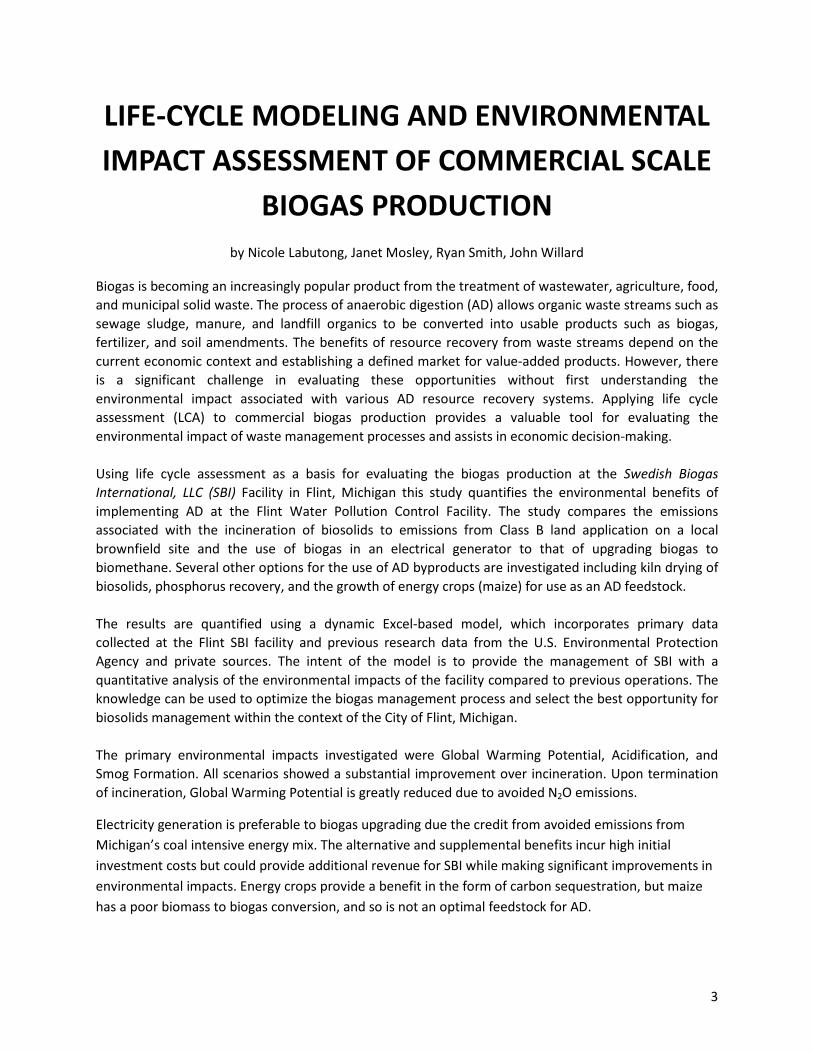
LIFE-CYCLE MODELING AND ENVIRONMENTAL IMPACT ASSESSMENT OF COMMERCIAL SCALE
BIOGAS PRODUCTION by Nicole Labutong, Janet Mosley, Ryan Smith, John Willard
Biogas is becoming an increasingly popular product from the treatment of wastewater, agriculture, food, and municipal solid waste. The process of anaerobic digestion (AD) allows organic waste streams such as sewage sludge, manure, and landfill organics to be converted into usable products such as biogas, fertilizer, and soil amendments. The benefits of resource recovery from waste streams depend on the current economic context and establishing a defined market for value-added products. However, there is a significant challenge in evaluating these opportunities without first understanding the environmental impact associated with various AD resource recovery systems. Applying life cycle assessment (LCA) to commercial biogas production provides a valuable tool for evaluating the environmental impact of waste management processes and assists in economic decision-making. Using life cycle assessment as a basis for evaluating the biogas production at the Swedish Biogas International, LLC (SBI) Facility in Flint, Michigan this study quantifies the environmental benefits of implementing AD at the Flint Water Pollution Control Facility. The study compares the emissions associated with the incineration of biosolids to emissions from Class B land application on a local brownfield site and the use of biogas in an electrical generator to that of upgrading biogas to biomethane. Several other options for the use of AD byproducts are investigated including kiln drying of biosolids, phosphorus recovery, and the growth of energy crops (maize) for use as an AD feedstock. The results are quantified using a dynamic Excel-based model, which incorporates primary data collected at the Flint SBI facility and previous research data from the U.S. Environmental Protection Agency and private sources. The intent of the model is to provide the management of SBI with a quantitative analysis of the environmental impacts of the facility compared to previous operations. The knowledge can be used to optimize the biogas management process and select the best opportunity for biosolids management within the context of the City of Flint, Michigan. The primary environmental impacts investigated were Global Warming Potential, Acidification, and Smog Formation. All scenarios showed a substantial improvement over incineration. Upon termination of incineration, Global Warming Potential is greatly reduced due to avoided N2O emissions.
Electricity generation is preferable to biogas upgrading due the credit from avoided emissions from Michigan’s coal intensive energy mix. The alternative and supplemental benefits incur high initial investment costs but could provide additional revenue for SBI while making significant improvements in environmental impacts. Energy crops provide a benefit in the form of carbon sequestration, but maize has a poor biomass to biogas conversion, and so is not an optimal feedstock for AD.

4
LIFE-CYCLE MODELING AND ENVIRONMENTAL IMPACT ASSESSMENT OF COMMERCIAL SCALE
BIOGAS PRODUCTION
UNIVERSITY OF MICHIGAN School of Natural Resources and Environment
Nicole Labutong
Janet Mosley
Ryan Smith
John Willard
April 2012
5
TABLE OF CONTENTS
Table of Contents .......................................................................................................................................... 5 Executive Summary ..................................................................................................................................... 12 1. Project Context and Study Goals ....................................................................................................... 17
1.1. Goals and Objectives ................................................................................................................... 17 1.2. Biogas Industry Background ........................................................................................................ 18 1.3. Introduction to Life Cycle Assessment ........................................................................................ 20 1.4. Intended Audience and Other Stakeholders .............................................................................. 22
2. System Description ............................................................................................................................. 23 2.1. Swedish Biogas Facility................................................................................................................ 23 2.2. Process Flow Diagrams ............................................................................................................... 24
2.2.1. Base Case ............................................................................................................................ 24 2.2.2. Current Operations ............................................................................................................. 24 2.2.3. Fully Operational ................................................................................................................. 25 2.2.4. Alternative and Supplementary Operations ...................................................................... 26 2.2.5. Description of Processes ..................................................................................................... 27
2.3. LCA Goals and Scope of the Study .............................................................................................. 31 2.3.1. Function and Functional Unit .............................................................................................. 32 2.3.2. System Boundaries .............................................................................................................. 32 2.3.3. Allocation Methods ............................................................................................................. 34 2.3.4. Data Requirements ............................................................................................................. 35 2.3.5. Impact Methods .................................................................................................................. 35
2.4. Software Interface ...................................................................................................................... 35 3. Methodology ...................................................................................................................................... 37
3.1. Multi-Criteria Decision Analysis .................................................................................................. 37 3.1.1. Introduction to MCDA ......................................................................................................... 37 3.1.2. Applications for Digestate ................................................................................................... 37 3.1.3. Criteria ................................................................................................................................. 39 3.1.4. Evaluation Technique .......................................................................................................... 39 3.1.5. MCDA Results ...................................................................................................................... 40
3.2. Background Research and Data Collection ................................................................................. 41 3.2.1. Swedish Biogas Facilities ..................................................................................................... 41 3.2.2. Air Emissions ....................................................................................................................... 42 3.2.3. Biosolids Management and EPA Regulations ..................................................................... 44
3.3. Modeling the Base Case .............................................................................................................. 44 3.4. Modeling the Biogas Production Process ................................................................................... 45
3.4.1. Transportation of Food Waste ............................................................................................ 46 3.4.2. Sludge Thickening ............................................................................................................... 46 3.4.3. Digestion ............................................................................................................................. 47 3.4.4. Digestate Storage ................................................................................................................ 49 3.4.5. Dewatering .......................................................................................................................... 50

6
3.4.6. Electricity Use ...................................................................................................................... 50 3.5. Investigating Biosolids and Centrate Management and Disposal .............................................. 51
3.5.1. Incineration ......................................................................................................................... 53 3.5.2. Brownfield Redevelopment: Class B, Chevy in the Hole ..................................................... 54 3.5.3. Kiln Drying ........................................................................................................................... 56 3.5.4. Energy Crops ....................................................................................................................... 57 3.5.5. Phosphorus Recovery: Ostara Pelletizer ............................................................................. 59
3.6. Modeling Biogas Usage ............................................................................................................... 61 3.6.1. Biogas Use in the Current operations ................................................................................. 61 3.6.2. Biogas Use in the Fully Operational Case ............................................................................ 61 3.6.3. Biogas Use for Alternative and Supplemental Operations ................................................. 63
3.7. System Expansion Allocation Methodology................................................................................ 63 3.7.1. Kiln Drying System Expansion ............................................................................................. 63 3.7.2. Phosphorus Recovery System Expansion ............................................................................ 64 3.7.3. Electricity Generation System Expansion ........................................................................... 65
3.8. Environmental Impact Assessment Modeling ............................................................................ 65 3.9. Conversion to Functional Unit .................................................................................................... 66 3.10. Biogenic Carbon ...................................................................................................................... 68 3.11. Sensitivity Analyses ................................................................................................................. 69
4. Results ................................................................................................................................................. 70 4.1. Life Cycle Inventory Analysis ....................................................................................................... 70
4.1.1. Base Case ............................................................................................................................ 70 4.1.2. Current Operations ............................................................................................................. 72 4.1.3. Fully Operational with Generator and Brownfield Application .......................................... 74 4.1.4. Fully Operational with Upgrader and Brownfield Application ............................................ 77 4.1.5. Fully Operational with Generator and Kiln Drying .............................................................. 79 4.1.6. Fully Operational with Generator and Use of Energy Crops ............................................... 81 4.1.7. Fully Operational with Generator and Phosphorus Recovery ............................................ 83 4.1.8. Non-Renewable Energy Use ................................................................................................ 85
4.2. Life Cycle Impact Assessment ..................................................................................................... 89 4.2.1. Global Warming Potential ................................................................................................... 89 4.2.1. Acidification Potential ......................................................................................................... 91 4.2.2. Smog Formation Potential .................................................................................................. 92
4.3. Sensitivity Analyses ..................................................................................................................... 94 4.3.1. Methane Production Potential, %VS of TS, and %VS Destruction ...................................... 94 4.3.2. Functional Unit: Dry Tons of Input ...................................................................................... 96
5. Additional Biosolid Management Scenarios ..................................................................................... 98 5.1. Pastuerization of Centrate to a Class A ....................................................................................... 98 5.2. Greenhouse Gas Emissions Reduction from Tree Plantation in CitH ......................................... 99 5.3. Class B – Land Application Farm/Forest .................................................................................... 100 5.4. Class A – Outdoor Composting ................................................................................................. 101 5.5. Class B – Superfund Sites .......................................................................................................... 102

7
5.6. Urban Agriculture ...................................................................................................................... 102 6. Discussion ......................................................................................................................................... 104
6.1. Optimal Allocation of Biosolids ................................................................................................. 104 6.2. Optimal Allocation of Biogas ..................................................................................................... 104 6.3. Alternate and Supplementary Cases ......................................................................................... 105
6.3.1. Kiln Drying ......................................................................................................................... 105 6.3.2. Phosphorus Recovery ........................................................................................................ 105 6.3.3. Energy Crops ..................................................................................................................... 105
6.4. Conclusion ................................................................................................................................. 106 7. Works Cited ...................................................................................................................................... 108 8. Appendices ....................................................................................................................................... 112
8.1. Appendix 1: MultiCriteria Decision Analysis ............................................................................. 112 8.2. Appendix 2: Emission Factors ................................................................................................... 113
8.2.1. Emission Factors for the Boiler ......................................................................................... 113 8.2.2. Emission Factors for the Incinerator ................................................................................. 115 8.2.3. Emission Factors for the Upgrader ................................................................................... 116 8.2.4. Emission Factors for the Flare ........................................................................................... 117 8.2.5. Emissions Factors for the Generator ................................................................................ 118 8.2.6. Emission Factors for the Michigan Electricity Grid ........................................................... 120
8.3. Appendix 3: Equipment and Electricity Use Tables .................................................................. 121 8.4. Appendix 4: Impact Characterization Factors ........................................................................... 123 8.5. Appendix 5: Sensitivity Analyses ............................................................................................... 123

8
LIST OF FIGURES Figure 1: Base Case ..................................................................................................................................... 24 Figure 2: Current Operations ...................................................................................................................... 24 Figure 3: Fully Operational .......................................................................................................................... 25 Figure 4: Alternative and Supplementary Operations ................................................................................ 26 Figure 5: Dashboard .................................................................................................................................... 36 Figure 6: MCDA Results ............................................................................................................................... 41 Figure 7: Base Case Greenhouse Gas Emissions ......................................................................................... 71 Figure 8: Base Case Criteria Pollutant Emissions ........................................................................................ 72 Figure 9: Current Operations Greenhouse Gas Emissions .......................................................................... 73 Figure 10: Current Operations Criteria Pollutant Emission ........................................................................ 74 Figure 11: Greenhouse Gas Emissions for Fully Operational with Generator ............................................ 76 Figure 12: Criteria Pollutant Emissions for Fully Operational with Generator ........................................... 76 Figure 13: Greenhouse Gas Emissions for Fully Operational with Upgrader ............................................. 78 Figure 14: Criteria Pollutant Emissions for Fully Operational with Upgrader............................................. 78 Figure 15: Greenhouse Gas Emissions for Fully Operational with Generator and Kiln Drying ................... 80 Figure 16: Criteria Pollutant Emissions for Fully Operational with Generator and Kiln Drying .................. 80 Figure 17: Greenhouse Gas Emissions for Fully Operational with Generator and Energy Crops ............... 82 Figure 18: Criteria Pollutant Emissions for Fully Operational with Generator and Energy Crops .............. 82 Figure 19: Greenhouse Gas Emissions for Fully Operational with Generator and Phosphorus Recovery . 84 Figure 20: Criteria Pollutant Emissions for Fully Operational with Generator and Phosphorus Recovery 84 Figure 21: Annual Natural Gas Consumption by Case ................................................................................ 85 Figure 22: Natural Gas Consumption per MCF of Biogas Produced by Case .............................................. 86 Figure 23: Annual Electricity Consumption by Case ................................................................................... 87 Figure 24: Electricity Consumption per MCF Produced by Case ................................................................. 87 Figure 25: Annual Diesel Consumption by Case ......................................................................................... 88 Figure 26: Diesel Consumption per MCF Produced by Case ....................................................................... 89 Figure 27: Annual Global Warming Potential by Case ................................................................................ 90 Figure 28: Global Warming Potential per MCF Produced by Case ............................................................. 90 Figure 29: Annual Acidification Potential by Case ...................................................................................... 91 Figure 30: Acidification Potential per MCF Produced by Case.................................................................... 92 Figure 31: Annual Smog Formation Potential by Case ................................................................................ 93 Figure 32: Smog Formation Potential per MCF Produced by Case ............................................................. 93 Figure 33. Sensitivity Analysis of Biogas Production in Current Operations .............................................. 94 Figure 34. Sensitivity Analysis of Global Warming Potential in Current Operations .................................. 94 Figure 35. Sensitivity Analysis of Biogas Production in Fully Operational with Generator ........................ 95 Figure 36. Sensitivity Analysis of Global Warming Potential in Fully Operational with Generator ............ 95 Figure 37. Global Warming Potential per Dry Ton of Input per Year.......................................................... 96 Figure 38. Acidification Potential per Dry Ton of Input per Year ................................................................ 97 Figure 39. Smog Formation Potential per Dry Ton of Input per Year ......................................................... 97 Figure 40. Sensitivity Analysis of Acidification Potential in Current Operations ...................................... 123 Figure 41. Sensitivity Analysis of Smog Formation Potential in Current Operations ............................... 124 Figure 42. Sensitivity Analysis of Acidification Potential in Fully Operational with Generator ................ 124 Figure 43. Sensitivity Analysis of Smog Formation Potential in Fully Operational with Generator ......... 125

9
LIST OF TABLES Table 1: Cell Color Description .................................................................................................................... 36 Table 2: Application of Anaerobic Digestion Products ............................................................................... 38 Table 3: Criteria Used to Evaluate Options for Digestate Application ........................................................ 39 Table 4: Biogas Composition, ...................................................................................................................... 49 Table 5: Initial Costs for Construction of Composting Facility at SBI .......................................................... 55 Table 6: Biomethane Composition.............................................................................................................. 62 Table 7: Elemental Analysis of Dewatered Biosolids .................................................................................. 64 Table 8: Crystal Green® Technical Data ...................................................................................................... 64 Table 9: Impact Assessment Midpoints ...................................................................................................... 66 Table 10: Base Case Dashboard .................................................................................................................. 70 Table 11: Base Case Input Values ............................................................................................................... 70 Table 12: Base Case Output Values ............................................................................................................ 71 Table 13: Current Operations Dashboard ................................................................................................... 72 Table 14: Current Operations Input Values ................................................................................................ 72 Table 15: Current Operations Output Values ............................................................................................. 73 Table 16: Dashboard for Fully Operational with Generator ....................................................................... 74 Table 17: Input Values for Fully Operational with Generator .................................................................... 75 Table 18: Output Values for Fully Operational with Generator.................................................................. 75 Table 19: Dashboard for Fully Operational with Upgrader......................................................................... 77 Table 20: Input Table for Fully Operational with Upgrader ........................................................................ 77 Table 21: Output Table for Fully Operational with Upgrader ..................................................................... 77 Table 22: Dashboard for Fully Operational with Generator and Kiln Drying .............................................. 79 Table 23: Input Table for Fully Operational with Generator and Kiln Drying ............................................. 79 Table 24: Output Table for Fully Operational with Generator and Kiln Drying .......................................... 79 Table 25: Dashboard for Fully Operational with Generator and Energy Crops .......................................... 81 Table 26: Input Table for Fully Operational with Generator and Energy Crops ......................................... 81 Table 27: Output Table for Fully Operational with Generator and Energy Crops ...................................... 81 Table 28: Dashboard for Fully Operational with Generator and Phosphorus Recovery ............................ 83 Table 29: Input Table for Fully Operational with Generator and Phosphorus Recovery............................ 83 Table 30: Output Table for Fully Operational with Generator and Phosphorus Recovery......................... 83 Table 31: Multi-Criteria Decision Analysis Criterion Weighting ................................................................ 112 Table 32: Boiler - Biogas Emission Factors Used in Model ....................................................................... 113 Table 33: Electrigaz Technologies Inc report for British Columbia Innovation Council 2008 ................... 113 Table 34: Stoichiometric Calculation for SOx Emissions from Biogas Combustion in Boiler .................... 114 Table 35: GREET1_2011 Emission Factors for Small Industrial Boiler ...................................................... 114 Table 36: Boiler – Natural Gas Emission Factors....................................................................................... 114 Table 37: Incinerator – Natural Gas Emission Factors .............................................................................. 115 Table 38: Incinerator – Biosolid Emission Factors Used in Model ............................................................ 115 Table 39: Incineration of Biosolids - Stoichiometric Emission Factor Calculations .................................. 116 Table 40: Upgrader - Emission Factors ..................................................................................................... 116 Table 41: Upgrader - Stoichiometric Calculation - H2S to SO2 ................................................................. 116 Table 42: Flaring – Biogas Emission Factors Used in the Model ............................................................... 117 Table 43: Electrigaz Technologies Inc report for British Columbia Innovation Council 2008 (Flaring) ..... 117 Table 44: Stoichiometric Calculation (Flaring) .......................................................................................... 118 Table 45: GREET1_2011 Emission Factors for Natural Gas Flaring in Oil Field ......................................... 118 Table 46. Generator – Biogas Emission Factors Used in the Model ......................................................... 118

10
Table 47. Generator - Emission Factors from Generator Specifications (Caterpillar G3520C, DM5740) . 119 Table 48. Generator - Emission Factors from Nielsen and Illerup (2003) ................................................. 119 Table 49. Generator - Stoichiometric Calculations ................................................................................... 119 Table 50: Electricity Grid - Emission Factors Used in the Model .............................................................. 120
TERMS AND ACRONYMS
%TS: Percent Total Solids
%VS Destroyed: Percent of Volatile Solids Destroyed During Digestion
%VS of TS: Percent Volatile Solids of Total Solids
AD: Anaerobic Digestion
AP: Acidification Potential
CHP: Combined Heat and Power
CitH: Chevy in the Hole
DT: Dry Tons
EPA: U.S. Environmental Protection Agency
Eq: Equivalent
GBT: Gravity Belt Thickener
GWP: Global Warming Potential
HRT: Hydraulic Retention Time
ISO: International Organization for Standardization
ISO: International Organization for Standardization
LCA: Life Cycle Assessment
MBtu: 1 Thousand British Thermal Units
MCDA: Multi-Criteria Decision Analysis
MCF: 1000 Standard Cubic Feet
MDEQ: Michigan Department of Environmental Quality
MGD: Million gallons per day
mmBtu: 1 Million British Thermal Units

11
Mol: Moles
MPP: Methane Production Potential
NPL: National Priorities List for Superfund Sites
NREPA: Natural Resources and Environmental Protection Act
PCOP: Smog Formation Potential
SBI: Swedish Biogas International
scf: Standard Cubic Feet
TRACI: Tool for the Reduction and Assessment of Chemical and Other Environmental Impacts
TS: Total Solids
VOCs: Volatile Organic Compounds
VS: Volatile Solids
WWTP: Wastewater Treatment Plant

12
EXECUTIVE SUMMARY
The University Of Michigan School Of Natural Resources and Environment Master’s Project program is an interdisciplinary problem-solving project conducted by Master’s students as a capstone for their academic degree. Swedish Biogas International (SBI) and a team of Master’s students initiated a research project focused on evaluating the environmental impacts of commercial scale biogas production using life cycle assessment (LCA).
The primary study goal is to offer insight into the benefits, drawbacks, and opportunities associated with operating a biogas facility at a large centralized wastewater treatment plant. The results are intended to offer credible quantitative and qualitative analyses on various alternatives for the management and application of biosolids as well as potential value-added products from biogas production.
Biogas is created through anaerobic digestion (AD) by bacteria called methanogens, which decomposing organic waste in an oxygen free environment to produce a mixture of methane, carbon dioxide, and sulfur. There are many different uses for biogas in the agricultural, sewage treatment, municipal solid waste, and transportation sectors. Anaerobic digesters produce gas, reduce solid waste, and provide valuable heat for pasteurization of digestate or centrate, heating and cooling, and in some cases electricity production. In sewage treatment plants biogas can be used to heat anaerobic digesters or produce electricity. Large scale biogas producers can also upgrade biogas to natural gas quality methane levels to be sold as an alternative transportation fuel also known as biomethane. The primary system in this study is the digestion of sewage sludge and food waste at the SBI biogas facility constructed at the Flint, Michigan Water Pollution Control Facility.
Life cycle assessment was the chosen method for evaluating biogas production systems and the byproducts associated with the process. The International Organization for Standardization (ISO) provides methodological guidelines and principles for carrying out and documenting a life cycle assessment. The ISO 14040 series defines four stages of an LCA: goal and scope definition, inventory analysis, impact assessment, and interpretation.
The primary function of the system was defined as production of usable energy in the form of biogas, therefore the functional unit of the system was defined as 1000 standard cubic feet (scf) or 1 MCF of biogas produced. Emissions and energy consumption were reported in the amount associated with the production of 1 MCF of biogas.
This will provide quantitative results that can assist SBI in making well-informed decisions based in part on how their business operations will impact the environment. The LCA will also allow SBI to communicate quantitatively the environmental benefits and tradeoffs associated with AD to the City of Flint and future clients.
FLINT, MICHIGAN SWEDISH BIOGAS FACILITY
The Swedish Biogas facility consists of two anaerobic digesters that were once utilized for the purpose of volatile solids destruction. These digesters were retired in the 1980s when incineration became the

13
primary means of biosolids disposal. In 2010, SBI retrofitted these digesters with new equipment to bring them up to operational status. The facility is currently processing about 9 dry tons of sludge per day with an expansion capacity of up to 24 dry tons per day when incorporating food waste as an additional input.
To illustrate and quantify the environmental impact of the plant’s operations and to provide useful recommendations for SBI, LCA methodology was used to determine the environmental impact of the plant’s operations in four cases:
BASE CASE
The Base Case describes Flint’s Wastewater Treatment Plant (WWTP) operations before any alterations were made by SBI. It serves as the baseline against which SBI’s environmental impact was measured. Sludge from the WWTP was pumped to a storage tank and dewatered from 3% to 23% total solids (%TS) using a belt filter press and polymers. Separated water (centrate) was then pumped back to the WWTP. The dewatered sludge was pumped to the incineration facility where it entered a series of incinerators, which further dewatered and combusted the sludge. The remains were cooled, forming ash, which was transferred via pipeline to an ash lagoon nearby for storage, then transported to a nearby Class II landfill two to three times per year.
CURRENT OPERATIONS
This case describes operations at the plant at the time the report was written (Spring 2012). Solids are removed from the primary settling tanks and the secondary clarifiers. A portion of the solids is thickened using a gravity belt thickener (GBT) and polymers, the GBT filtrate and centrate is returned to the head of the WWTP. The volume to be thickened is determined by the allowable daily volume of input. Unthickened sludge is mixed with thickened sludge before being pumped through a heat exchanger to be digested. In the heat exchanger, sludge from the WWTP is pre-heated by material exiting the digester. The current volume of sludge input only requires use of one of the two digesters in the facility. Biogas produced is used in a boiler to heat the digestion process. The biosolids remaining after digestion (digestate) are dewatered by a centrifuge and incinerated.
FULLY OPERATIONAL
The Fully Operational case describes SBI’s future plans as of March 2012. In addition to sludge from the WWTP, SBI will include food waste from local food manufacturing plants, grocery stores, and farms, which will be transported to SBI via truck. Due to the increased volume of input, two digesters will be utilized. Since food waste has a greater percentage of volatile solids, there will be an increase in biogas production. Instead of incineration, the dewatered digestate will be transported via truck to a vacant manufacturing complex known as Chevy in the Hole (CitH). CitH is a brownfield spanning 130 concrete-covered acres located across the street from the SBI offices. The biogas can be utilized in internal combustion for the purposes of combined heat and power (CHP) generation. Electricity can be sold to the grid and excess heat from the generator can be directed

14
toward the heat exchanger and the digester. Biogas can also be upgraded to biomethane and distributed via natural gas pipelines or used in a vehicle fleet.
ALTERNATIVE AND SUPPLEMENTARY OPERATIONS
Additional scenarios applicable to the Fully Operational case were investigated. While SBI is moving forward with land application at CitH as the primary biosolids disposal option, there are a number of alternatives to disposal that can be considered as contingencies as well as several additions to the plan that could be carried out in conjunction with CitH. The master’s project team investigated three options. The first option was an alternative biosolids disposal option that could be employed in place of CitH. The second option addressed the use of GBT filtrate and centrate, another byproduct of AD, and could be carried out regardless of the biosolids disposal method. The third option could only be implemented in addition to CitH.
KILN DRYING
The digestate is heated to high temperatures using a kiln dryer to remove pathogens in order to meet Class A standards set by the EPA and to possibly be sold as a soil amendment in the form of dry compost. This is done in place of applying digestate to CitH.
PHOSPHORUS RECOVERY
Gravity belt thickener filtrate and the centrate from the centrifuge are sent to a PEARL® Reactor (Ostara © Nutrient Recovery Technologies). The reactor separates, dries and pelletizes a slow release fertilizer product trademarked as Crystal Green ©. The Crystal Green© product is then marketable as a slow release fertilizer.
ENERGY CROPS
SBI could grow energy crops at CitH that could be used to supplement their inputs for anaerobic digestion. Corn, already a thriving crop in the region, could be annually grown and ensiled for storage and AD pre-treatment. The corn could then be mixed with sludge and/or other food waste before being pumped through the heat exchanger to the digesters.
MULTI-CRITERIA DECISION ANALYSIS
Given limited resources to investigate myriad of biogas use, digestate disposal or value-added alternatives that exist, multi-criteria decision analysis (MCDA) was employed to help narrow down and identify the most valuable areas of research.
The criteria used to evaluate the options were factors predicted to affect SBI’s development as a company, relevant to SBI’s mission and in compliance with applicable regulations. These factors address

15
the triple bottom line: economics, society, and the environment. Additionally, the feasibility of the options based on current and predicted future conditions were evaluated.
ENVIRONMENTAL IMPACT ASSESSMENT MODEL
In order to develop a comprehensive life cycle assessment that evaluated multiple system boundaries, inputs and outputs, we developed an Excel-based model that could dynamically calculate the comparisons between the Base Case, Current Operations, Fully Operational and Alternative and Supplementary cases. This model contains a dashboard that allows the user to manipulate flows into the system and allocate the biogas and digestate products to the various systems incorporated in the model. The model then allowed us to generate results and perform sensitivity analyses for each scenario.
RESULTS
The key results of the study were based on three environmental impact indicators: Global Warming Potential (GWP), Acidification Potential (AP), and Smog Formation Potential (PCOP). The results show that current, fully operational, alternative and supplemental operations performed substantially better than Base Case in all indicators.
In accounting for GWP per MCF, all cases showed substantial improvements from the Base Case. The reductions ranged from nearly 1000 lb CO2 eq/MCF for the current operations to roughly 5,700 lb CO2 eq/MCF for energy crops and phosphorus recovery Figure 28. A majority of the improvements are attributed to a reduction in emissions from biogenic sources.
All cases showed avoided acidification potentials compared to the Base Case. These improvements from the Base Case ranged from approximately -12 mol H+ eq/MCF for Fully Operational with Upgrader to -38 mol H+ eq/MCF for phosphorus recovery.
All cases showed avoided biogenic and non-biogenic smog formation potentials per MCF of biogas relative to the Base Case. Values ranged from about -2 lb O3 eq/MCF in the current operations and -16 lb O3 eq/MCF in phosphorus recovery.
CONCLUSIONS
This report recommends that biogas should be allocated to generate electricity rather than upgraded to biomethane. This option not only reduces emissions, but also is suited to market conditions in the United States. In Sweden electricity is much cheaper and is produced from hydropower and nuclear power, which are much less carbon intensive compared to the grid mix in Michigan. The higher cost of electricity in the U.S. makes it more financially attractive to generate electricity.
While SBI has been successful in working with municipal governments to create a biogas-driven public transportation fleet in Linköping, it would be much more difficult to do so in Flint. First, diesel fuel in Sweden is roughly twice as expensive as gasoline in the U.S. Second, while the City of Flint government

16
may find it environmentally beneficial to implement a green public transportation fleet, the city has neither the concentrated infrastructure nor a sufficient population to make this viable.
A number of biosolids application options are dependent on available financial capital. While SBI’s partnership with the COF has aided in producing revenue, the city’s financial crisis limits the projects SBI can engage in. Currently, an economic emergency manager is auditing and restructuring Flint’s operations and investments. Though many of the potential projects would eventually provide a return of investment, their payback period is longer than desired. Investments in projects with high capital are not feasible at this time. Kiln drying, phosphorus recovery, and energy crops can reduce negative environmental impact. However, since they are not economically viable they cannot implement. In sum, “you have to be in the black to be green.”

17
1. PROJECT CONTEXT AND STUDY GOALS
The context of this project is centered on providing the client, Swedish Biogas International (SBI), with a valuable and comprehensive analysis of environmental impacts associated with the production of biogas. The project is geographically focused on the biogas facility in Flint, Michigan with the goal of generating a knowledge base for the construction of future facilities in the United States. The primary researchers for this project, referenced from this point forward as the “master’s project team,” is comprised of four Masters Students at the University of Michigan’s School of Natural Resources and Environment.
The primary study goal is to offer insight into the benefits, drawbacks, and opportunities associated with operating a biogas facility at the City of Flint (COF) wastewater treatment plant (WWTP). The results are intended to offer credible quantitative and qualitative analyses on various alternatives for the management and application of biosolids as well as potential value-added products from biogas production.
1.1. GOALS AND OBJECTIVES
The goal of this project is to quantify the environmental impact of the Swedish Biogas International facility in Flint, Michigan and evaluate it against the baseline environmental impacts of the Flint Water Pollution Control Facility’s biosolids disposal operations. In addition, this study investigates the various applications of biogas within the system and utilizes life cycle assessment (LCA) to identify value added products from the biogas production process.
The specific primary objectives of this project are as follows:
• Construct a user-friendly, modular, easy-to-understand, life-cycle assessment tool that quantifies energy consumption, fuel production, and air emissions from the Swedish Biogas facility to validate the merits of anaerobic digestion (AD) for Swedish Biogas, the environment, and for the City of Flint.
• Identify and evaluate a range of options for disposal or application of biosolids, centrate, and biogas. Options included in the model:
- Delivering biosolids to Chevy in the Hole (CitH), a nearby brownfield site at which biosolids will be used for bioremediation.
- Upgrading the Class B biosolids to Class A biosolids via kiln drying, and selling the upgraded product as an organic fertilizer for agricultural and other landscaping applications.

18
- Growing energy crops on selected plots of land at CitH to be used as supplemental input for anaerobic digestion
- Installing nutrient recovery technology to a recover phosphorus and create a value-added fertilizer product from the centrate that would otherwise return to the head of the wastewater treatment plant.
Additional options for biosolids application that may be applied in addition to or instead of current operations at the plant will be evaluated but not included in the model.
• Deliver an executable version of our LCA model and a final report that summarizes our findings and recommendations to Swedish Biogas International.
This report is intended to provide a summary of our model construction, analysis methods and evaluation of alternative applications of the byproducts from anaerobic digestion.
1.2. BIOGAS INDUSTRY BACKGROUND
Biogas creation at wastewater treatment plants is an old but under-utilized technology. The application of biogas first became apparent in the 1800s in London when gas from the sewers was burned in street lamps. Originally, biogas was a byproduct of a process developed to reduce volatile solids at early centralized sewage treatment plants in Europe in the early 1900s. Agricultural production of biogas was developed in India in the 1930s for the purpose of providing cooking fuel to remote villages. Energy shocks in the 1970s and the rising price of oil in the early 1980s led to further implementation of biogas in Europe as an alternative source of energy. Today there are over 1,300 large (greater than one million gallons per day [MGD]) wastewater treatment plants in the United States operating with anaerobic digestion. This accounts for about 43% of all wastewater treatment facilities in the same range.1 Other sources of biogas include landfill gas or methane collected from capped landfill sites where a significant amount of organic material exists.
Biogas is created through anaerobic digestion by bacteria called “methanogens” that decompose organic waste in an oxygen free environment to produce a mixture of methane, carbon dioxide, and sulfur. AD involves four steps: hydrolysis, acidification, acetic acidification, and methane generation. Hydrolysis involves the breakdown and liquefaction of organic matter by bacteria, this process results in free floating sugars, amino acids, peptides and fatty acids. Acidification follows with acid-forming bacteria breaking down the material from the hydrolysis stage; the results include volatile organic compounds, carbon dioxide, hydrogen and ammonia. The next stage, acetic acidification, converts
1 U.S. EPA, C. H. (2011, October). Opportunities for Combined Heat and Power at Wastewater Treatment Facilities. http://www.epa.gov/chp/documents/wwtf_opportunities.pdf

19
volatile organic compounds into acetic acid (CH3COOH) and CO2. In the final stage methanogens convert the acetic acid into methane (CH4). The result is a stable gas yield of carbon dioxide, methane, and hydrogen sulfide (CO2, CH4, H2S respectively). Gas composition can vary significantly depending on the process conditions and feedstock. Landfill gas typically has a methane content of 50-55%, whereas sewage and manure feedstock produce around 60-75% methane content.2
Human and animal waste provides a more consistent feedstock for anaerobic digestion. Landfill gas is much less controlled and therefore contains higher levels of hydrogen sulfide as well as other trace elements of chlorine and fluorine. Siloxanes are also an important factor in biogas composition because of the white powder coating that forms in gas turbines, heat exchangers and deposits in reciprocating engines, causing increased maintenance costs.3
There are many different uses for biogas in the agricultural, sewage treatment, municipal solid waste, and transportation sectors. Agricultural digesters produce gas to reduce manure and provide valuable heat for pasteurization, heating and cooling, and in some cases electricity production. In sewage treatment plants biogas can be used to heat the anaerobic digestion process and surrounding buildings or produce electricity. Municipal solid waste facilities harness methane gas from decomposing organic matter from capped landfills through a network of piping systems. The gas is often used to generate electricity, which generates additional revenue for landfill operators. In third world countries biogas is becoming an increasingly used method of sanitizing human waste and providing a source for cooking and lighting fuel. Large-scale biogas producers can upgrade biogas to natural gas quality methane levels to be sold as an alternative transportation fuel also known as biomethane.
Making biogas production economically viable depends on a multitude of political, economic, and geographic factors. In Europe, transportation fuel prices are significantly higher than in the U.S. making biomethane the most economically feasible use of biogas. In Sweden, biogas for the purpose of electricity production is unable to compete with the low cost of near-carbon-free sources of hydroelectric and nuclear power. In the U.S., wastewater treatment plants use biogas as a means to conduct peak shaving (reduced metering demand by producing onsite electricity) to bring about significant cost savings.4
2 U.S. DOE. “What is Emerging Biogas?” Alternative Fuels & Advanced Vehicles Data Center. Web. <http://www.afdc.energy.gov/afdc/fuels/emerging_biogas_what_is.html>.
3 Wheless, E., J. Pierce. “Siloxanes in Landfill and Digester Gas Update.” 2004. Web. <http://www.scsengineers.com/Papers/Pierce_2004Siloxanes_Update_Paper.pdf>.
4 Power Engineering. “Vermont Wastewater Treatment Facility to Generate Its Own Heat and Power from Digester Gas." 27 Mar. 2012. Web. <http://www.power-eng.com/articles/2003/03/vermont-wastewater-treatment-facility-to-generate-its-own-heat-and-power-from-digester-gas.html>.

20
1.3. INTRODUCTION TO LIFE CYCLE ASSESSMENT
Life cycle assessment is a method to quantify and characterize the environmental impacts from all processes in each stage of a product’s5 life including raw material acquisition, production, use, and disposal. The International Organization for Standardization provides methodological guidelines and principles for carrying out and documenting a life cycle assessment. Here we reference the 1997 ISO 14040 series.6 ISO 14040 defines four stages of an LCA: goal and scope definition, inventory analysis, impact assessment, and valuation.
GOAL AND SCOPE DEFINITION
The goal and scope of the LCA outlines the purpose of the study, defines the product, the boundaries of the system under consideration, and data requirements. Goal definition requires the LCA practitioner to clearly state the intended application and users of the LCA results.
Scope definition addresses:
• Product system to be studied • Function of the product system • Functional unit of the product system • Product system boundaries • Allocation methods • Types of impact and methodology of impact assessment • Data requirements, assumptions, and limitations
The LCA process is iterative, and as such, the scope may be revised over the course of the inventory analysis, impact assessment, and interpretation.
FUNCTION AND FUNCTIONAL UNIT
The function defines the service provided by the product system. A system may have several functions, and the function defined should be related to the goals of the study. The functional unit specifies a reference to which the system inputs and outputs are related.
SYSTEM BOUNDARIES
The system boundaries indicate which unit processes the study will include. Assumptions, cut-off criteria based on mass, energy, or environmental significance, and limited time and monetary resources, as well
5 “Product” in this context also refers to services
6 ISO. ISO 14040: Environmental Management - Life Cycle Assessment - Principles and Framework. Tech. 2nd ed. ISO, 2006. Print.

21
as the intended audience contribute to the boundary definition. The scope must include justification for the selected boundaries.
ALLOCATION METHODS
A system can have multiple products, thus requiring procedures to allocate the appropriate share of materials and energy flows and associated environmental releases to the product of interest. Allocation may be performed on a mass, volume, economic, or energy basis. However, it is best to avoid allocation through system expansion or division of processes into product specific sub-processes.
DATA REQUIREMENTS
Data quality requirements provide guidelines for acceptable data for the study. Data requirements should encompass:
• Time-related coverage • Geographical coverage • Technology coverage • Precision, completeness, and representativeness of the data • Consistency and reproducibility of the methods used throughout the LCA • Uncertainty in the data
INVENTORY ANALYSIS
The inventory analysis includes data collection and calculations to quantify the material and energy flows in and out of the system. The inventory analysis is the input to the impact assessment phase, but interpretation of the inventory results may also occur, depending on the goals and scope of the study.
As the LCA practitioner collects more data and learns more about the product system, the goals and scope should be revisited and may be modified if necessary.
IMPACT ASSESSMENT
The life cycle impact assessment attempts to equate the inputs and outputs calculated in the inventory analysis with human health and environmental impacts. The first step, classification, involves assigning inventory results to appropriate impact categories. The second step, characterization, involves modeling the inventory data to determine the magnitude of each type of environmental impact.
As the LCA practitioner carries out the impact assessment, issues may arise that require modifications to the goals and scope of the project.
INTERPRETATION
In this step, the inventory analysis and/or the impact assessment results are examined according to the goals of the study. Life cycle assessment results may be used to:
22
• Identify the most significant types of environmental impact, at which stages the impacts occur, and opportunities for improvement of the system.
• Help in a decision-making process such as product design, planning, or policy creation • Support marketing claims
LIMITATIONS OF LCA
While LCA is a powerful tool intended to comprehensively assess a product’s environmental impact, LCA is a new and evolving methodology with several limitations. First, assumptions and choices made, such as system boundaries and data source selection, are often subjective and can significantly affect the accuracy of the results of the study. Second, the data necessary for an accurate assessment may not exist or be accessible. Third, an LCA carried out on one scale, e.g. global, may not be generalized to another scale, e.g. local. Finally, LCA does not currently consider temporal or spatial dimensions, which may introduce significant uncertainty when modeling the environmental impacts.
1.4. INTENDED AUDIENCE AND OTHER STAKEHOLDERS
This study and its results are primarily for the use of Swedish Biogas International, LLC to assist in the evaluation of options for the use of the products and byproducts of anaerobic digestion in Flint and other future projects. As the wastewater treatment plant at Flint, Michigan is operated in conjunction with the City of Flint, we also expect City of Flint officials and employees to review the results and their implications. SBI’s parent company, Swedish Biogas International AB, in Sweden will be provided with a copy of the report, as well. Furthermore, other municipalities evaluating their biosolids management options may seek access to this report to help inform their biosolids management decisions.
Stakeholders also include the members of the Flint community and supporters of renewable energy generation. As the taxpayers who fund the operation of the wastewater treatment plant, City of Flint residents have a financial stake in how money is spent to manage the biosolids. Some of the projects proposed in this study have the potential for positive health and social impacts for residents. Many environmentalists are eager to understand the potential of biogas as a source of local, renewable energy and to learn how the system may be optimized for specific sites.

23
2. SYSTEM DESCRIPTION
The Flint Wastewater Treatment Plant is located five miles west of downtown Flint, Michigan. The plant has a 55 million gallon per day capacity and comprises primary and secondary treatment processes. The plant utilizes conventional activated sludge treatment where solids are removed from the primary and secondary treatment processes. The current load of the plant averages approximately 19 million gallons per day, or about 35% of the total capacity of the plant’s design.7 The typical solids handling load is approximately 7.5 dry tons per day. Before operations with Swedish Biogas International, the plant utilized multiple hearth incineration as a means of biosolids disposal followed by depositing the ash in an ash lagoon located adjacent to the facility. The ash was then transported to a landfill.
2.1. SWEDISH BIOGAS FACILITY
The Swedish Biogas (SBI) facility consists of two anaerobic digesters that were once utilized for the purpose of volatile solids destruction. These digesters were retired in the 1980s when incineration became the primary means of biosolids disposal. In 2010, SBI retrofitted these digesters with new equipment to bring them up to operational status. The system is comprised of two in-ground tanks that are 80 feet in diameter, measuring 26.5 feet high and have a storage volume of 940,000 gallons each. SBI utilizes a gravity belt thickener capable of processing 1,651 pounds per hour with a 95% solids capture rate. The sludge is thickened to a concentration of ~6% total solids, which is pumped into the digester with a 53 gallon per minute transfer pump. Inside the digester the sludge is mixed with two jet-mixing systems capable of pumping 3,840 gallons per minute. Digestion has a typical retention time of 20-30 days. Digested sludge, or digestate, is then transferred to a 270,000 gallon storage tank, which is mixed by two horizontal tank mixers. Digestate is then dewatered using a centrifuge, with a solids capture rate of 95%. Dewatered solids, or cake averages approximately 26% solids. Various methods of biosolids disposal are discussed in Section 3.5.
7 U.S. EPA. “Discharge Monitoring Report (DMR) Pollutant Loading Tool.” (2010) Web. <http://cfpub.epa.gov/dmr/>.

24
2.2. PROCESS FLOW DIAGRAMS
2.2.1. BASE CASE
Figure 1: Base Case
2.2.2. CURRENT OPERATIONS
Figure 2: Current Operations
WWTP Incineration Ash TransportationAsh LagoonSludge
Dewatering Landfill
Heat Exchange
WWTP
Digestion
Digestate Storage
Boiler
DewateringSludge Thickening Incineration Ash
TransportationAsh Lagoon Landfill
Heat Exchange
Current
Contingency/Supplementary
Outside of Boundaries
Heat Transfer
25
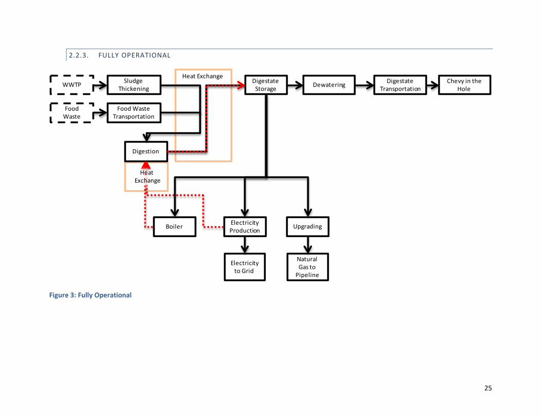
2.2.3. FULLY OPERATIONAL
Figure 3: Fully Operational
Heat ExchangeWWTP
Food Waste
Food Waste Transportation
Digestion
Digestate Storage
Electricity Production
Electricity to Grid
Upgrading
Natural Gas to
Pipeline
Chevy in the Hole
Digestate Transportation
Boiler
DewateringSludge Thickening
Heat Exchange
26
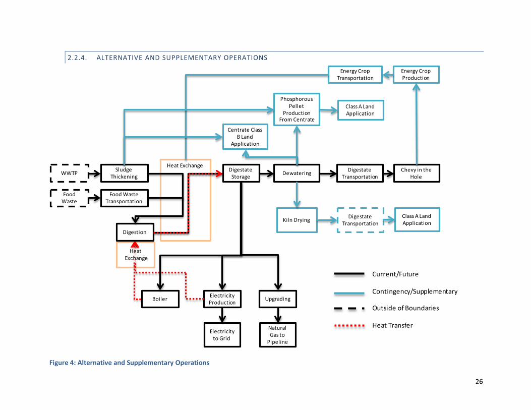
2.2.4. ALTERNATIVE AND SUPPLEMENTARY OPERATIONS
Heat ExchangeWWTP
Food Waste
Food WasteTransportation
Digestion
Digestate Storage
Electricity Production
Electricity to Grid
Upgrading
Natural Gas to
Pipeline
Chevy in the Hole
Digestate Transportation
Boiler
DewateringSludge Thickening
Centrate Class B Land
Application
Phosphorous Pellet
Production From Centrate
Class A Land Application
Energy Crop Production
Energy Crop Transportation
Kiln DryingClass A Land Application
Heat Exchange
Digestate Transportation
Current/Future
Contingency/Supplementary
Outside of Boundaries
Heat Transfer
Figure 4: Alternative and Supplementary Operations

27
2.2.5. DESCRIPTION OF PROCESSES
To better illustrate and quantify the environmental impact of the plant’s operations and to provide useful recommendations for SBI we measured the environmental impact of the plant’s operations in four cases:
1. Base Case 2. Current Operations 3. Fully Operational 4. Alternative and Supplementary Operations
a. Kiln Drying b. Energy Crops c. Phosphorus Recovery
Using these four cases we investigate the electric, thermal and material inputs and outputs from each system setup. Provided below is a brief description of each scenario and the processes involved. Results from the empirical and modeling data are provided in Section 4.
2.2.5.1. BASE CASE
The Base Case describes Flint’s Wastewater Treatment Plant (WWTP) operations before any alterations were made by SBI. It serves as the baseline against which we measure SBI’s environmental impact. A schematic of the operations is outlined in Figure 1.
Sludge from the WWTP was pumped to a storage tank and dewatered from 3% to 23% total solids (%TS) using a belt filter press and polymers. Separated water was then pumped back to the WWTP. The dewatered sludge was pumped to the incineration facility where it entered a series of incinerators, which further dewatered and combusted the sludge. The remains were cooled, forming ash. The incinerators, which require natural gas, were very energy intensive (heating the sludge to over 1000° F) and emitted a substantial amount of greenhouse gases. It also accounted for a large amount of operational costs at approximately $500,000 per year. The ash was then transferred via pipeline to an ash lagoon across the street for storage then transported to a Class II landfill two to three times per year.
2.2.5.2. CURRENT OPERATIONS
This case describes operations at the plant at the time the report was written (Spring 2012). A schematic of the operations is outlined in Figure 2.
SBI’s introduction did not alter any treatment operations at the neighboring wastewater treatment facility. Solids are removed from the primary settling tanks and the secondary clarifiers. A portion of the solids is thickened to ~6% solids using a gravity belt thickener (GBT) and polymers, the GBT filtrate is returned to the head of the WWTP. The volume to be thickened is determined by the allowable daily

28
volume of input (see Section 3.4.2). Unthickened sludge is mixed with thickened sludge before being pumped through a heat exchanger to be digested. In the heat exchanger, sludge from the WWTP is pre-heated by material exiting the digester. The current volume of sludge input only requires use of one of the two digesters in the facility. The biosolids remaining after digestion are then dewatered by a centrifuge and incinerated.
ANAEROBIC DIGESTION
In anaerobic digestion, bacteria decompose the volatile organic materials in the sludge to produce biogas consisting of 50-80% methane (CH4), 20-50% carbon dioxide (CO2), and small amounts of nitrous oxide (N20), hydrocarbons (HCs), sulfur oxides (SOx), nitrous oxides (NOx), carbon monoxide (CO), and volatile organic compounds (VOCs).8 The remaining solid material is referred to as digestate or anaerobically digested biosolids.
Several conditions should be met to optimize anaerobic digestion. The process must be carried out in the absence of oxygen (anaerobic) and at a constant temperature between 98-130° F. SBI utilizes mesophillic conditions (~98° F), as they are the most stable and commonly used for commercial operations. The sludge should have a certain range of water to solids, have a C-N ratio between 10-30, have a certain pH, and be mixed to ensure consistency and aids the bacteria.9 The retention time at SBI was optimized to 20 days for sludge in order to produce the largest volume of biogas over the shortest period of time.
The warmed digestate is pumped from the digester through the heat exchanger to pre-heat incoming sludge to a storage tank. In storage some gas production still occurs, though at a much slower rate than in the digester. A blower moves the gas to a hot water boiler, which is used to heat the digester. Excess gas is flared. Digestate is pumped to the incinerator and operations are carried out as described in the Base Case.
2.2.5.3. FULLY OPERATIONAL
The Fully Operational case describes SBI’s future plans as of March 2012, which has yet to be implemented. Processes not described below are the same as in the current operations case. A schematic of the operations is outlined in Figure 3.
In addition to sludge from the WWTP, SBI will include food waste from local food manufacturing plants, grocery stores, and farms, which will be transported to SBI via truck. The %TS of the food waste will vary, though SBI approximates it at ~10-15%.10 Therefore, the food would not likely be thickened. It will
8 Energy Savers. "How Anaerobic Digestion (Methane Recovery) Works." Energy Savers. Web. 15 Apr. 2012. <http://www.energysavers.gov/your_workplace/farms_ranches/index.cfm/mytopic=30003>.
9 Ibid. 10 Anna Brynas. Personal e-mail communication. 29 March 2012.

29
be mixed with the sludge and pumped to the heat exchanger. Due to the increased volume of input, both digesters (North and South) will be utilized. Since food waste has a greater percentage of volatile solids, there will be an increase in biogas production.
Instead of incineration, the digestate will be transported via truck to a vacant manufacturing complex known as Chevy in the Hole (CitH). CitH is a brownfield spanning 130 concrete-covered acres located across the street from the SBI offices.
The digestate will be land applied separately from local yard waste. SBI will work with the City of Flint to turn CitH into a park, as part of a larger effort to revitalize the Flint, Michigan. SBI and the City of Flint have also discussed the possibility of expanding to other brownfields in and around Flint once the transformation of CitH is completed, though there are no set plans.
In addition to supplying fuel for the boiler, biogas from storage will be upgraded and sold as biomethane to the natural gas pipeline or converted to electricity and sold to the grid. Upgrading biogas to biomethane increases the percentage of methane in the gas from ~65% to 98%. In Sweden, SBI primarily uses water scrubbing as an upgrading technology, requiring water and electricity as inputs. Stripped air, which includes gases that are removed in upgrading, consists mainly of CO2 and some other gases found in biogas and are emitted to the atmosphere. The upgraded biomethane can be sold into the natural gas pipeline, or as a vehicle transportation fuel.
The biogas can also be utilized in internal combustion for the purposes of combined heat and power (CHP) generation. Biogas has a heating value of approximately 60% of natural gas and can be burned in generators that take both fuels. Electricity can be sold to the grid and excess heat from the generator can be directed toward the heat exchanger and the digester.
2.2.5.4. ALTERNATIVE AND SUPPLEMENTARY OPERATIONS
Three additional scenarios applicable to the Fully Operational case were investigated and are described below. While SBI is moving forward with composting at CitH as the primary biosolids disposal option, there are a number of alternatives to disposal that can be considered as contingencies as well as several additions to the plan that could be carried out in conjunction with CitH. The master’s project team decided to study three options. The first option was an alternative biosolids disposal option that could be employed in place of CitH. The second option addressed the use of GBT filtrate and centrate, another byproduct of AD, and could be carried out regardless of the biosolids disposal method. The third option could only be implemented in addition to CitH.
The investigation of the alternative to CitH was undertaken for a few reasons. First, there remains a small risk that CitH composting operations will not come to fruition, due to ever-changing political, economic, and social motivators in the City of Flint area. Second, it would be helpful for SBI to be aware of a range of options for biosolids disposal, to give the organization an intellectual advantage on its competitors in the biogas space. Third, since the CitH composting operation may reach its end-of-life in 10 years’ time, it will be beneficial for SBI to know the other feasible long-term alternatives so it can

30
continue to operate far into the future. See to visualize how these optional projects would work within the Fully Operational scenario.
2.2.5.4.1. KILN DRYING
In this system process, the digestate is heated to high temperatures using a kiln dryer to remove pathogens in order to meet Class A standards set by the EPA and to possibly be sold as a soil amendment in the form of dry compost. This is done in place of applying digestate to CitH. Though anaerobic digestion removes up to 95-98% of pathogens, the Environmental Protection Agency (EPA) requires 100% pathogen removal for biosolids to be considered safe for human contact or land application.11 Heating the digestate to one of four temperature treatments defined by the EPA to receive Class A classification will allow the biosolids to be applied with less stringent regulations.12
The kiln dryer, which runs on natural gas or biogas, heats digestate to over 122° F for at least 20 minutes at the rate of 1 ton per hour, as required by the EPA to meet minimum Class A standards.13 In this operation, biogas would be burned as the heat source for the kiln drier. After the pathogens are destroyed, the biosolids would move through a serious of baffles that would fluff the material. The fertilizer would then move through a series of screens to filter particles to a desired size. The organic fertilizer would be stored in a silo until it is ready for transportation to a packaging facility.
The system boundaries to this system are described in Section 2.3.2.4.1
2.2.5.4.2. PHOSPHORUS RECOVERY
Anaerobic digestion can increase the concentration of soluble phosphorus in the centrate being returned to the wastewater treatment plant. Nutrient recovery technologies such as the Ostara’s PEARL® process can recover valuable nutrients such as phosphorus and magnesium from the centrate and convert them into a slow release fertilizer product.
The system process involves pumping the filtrate from the gravity belt thickener and the centrate from the centrifuge is sent to the PEARL® Reactor (Ostara® Nutrient Recovery Technologies). The reactor separates, dries and pelletizes a slow release fertilizer product trademarked as Crystal Green®. The Crystal Green® product is then marketable as slow release fertilizer. In order to quantify the
11 Michigan State University. "Pathogen Reduction in Anaerobic Digestion of Manure - Extension." Extension.org. Web. 15 Apr. 2012. <http://www.extension.org/pages/30309/pathogen-reduction-in-anaerobic-digestion-of-manure>.
12 U.S. EPA. "A Plain English Guide to the EPA Part 503 Biosolids Rule." Home. Web. 02 Apr. 2012. <http://water.epa.gov/scitech/wastetech/biosolids/503pe_index.cfm>.
13 U.S. EPA. "Pathogen and Vector Attraction Reduction Requirements." U.S. EPA. Web. <http://water.epa.gov/scitech/wastetech/biosolids/upload/2002_06_28_mtb_biosolids_503pe_503pe_5.pdf>.

31
environmental benefit of phosphorus recovery a system expansion of the LCA was used to compare the recovered phosphorus with that of mined phosphorus, equating each ton of available phosphorus to the cradle-to-gate life-cycle of virgin phosphorus.
The system boundaries to this system are described in Section 2.3.2.4.2
2.2.5.4.3. ENERGY CROPS
Contingent upon composting the digestate at CitH, SBI would have up to 130 acres of arable land.14 SBI could grow energy crops at CitH that could be used to supplement their inputs for anaerobic digestion. Corn, already a thriving crop in the region, should be annually grown and stored in a silo in which controlled fermentation can take place. The ensiling process preserves crops and has been known to increase methane production in corn. 15 The ensiled corn could then be ground and mixed with sludge and/or other food waste before being pumped through the heat exchanger to the digesters. Estimated yields are 8 wet tons per acre per year, with ~0.085 MCF biomethane/dry ton.16,17
The system boundaries to this system are described in Section 2.3.2.4.3
2.3. LCA GOALS AND SCOPE OF THE STUDY
The goal of this LCA is to provide SBI with information on how their operations impact the environment:
1. In comparison with operations before adding the anaerobic digestion system (Base Case) 2. Upon application of different scenarios of digestate disposal 3. Upon application of several scenarios of biogas utilization 4. Upon application of various scenarios of AD byproduct utilization
This will provide quantitative results that can assist SBI in making well-informed decisions on how their business operations will impact the environment. The LCA will also allow SBI to communicate
14 SNRE. "Reimagining Chevy in the Hole." University of Michigan School of Natural Resources and Environment. 2 Apr. 2012. Web. <http://www.thelandbank.org/Landuseconf/Reimagining_Chevy_in_the_Hole.pdf>.
15 Amon, Thomas, Vitaliy Kryvoruchko, Barbara Amon, Werner Zollitsch, Erich Potsch. "Biogas Production from Maize and Clover Grass Estimated With the Methane Energy Value System." Web. <http://www.boku.ac.at/fileadmin/_/H93/H931/AmonPublikationen/biogas_production_maize_and_clover.pdf>.
16 USDA. “2007 Census of Agriculture.” U.S. Department of Agriculture. 2007. Web. <http://www.agcensus.usda.gov/Publications/2007/Full_Report/usv1.pdf>.
17 Oslaj, Matjaz, Bogomir Mursec, and Peter Vindis. "Biogas Production from Maize Hybrids." Biomass and Bioenergy 34.11 (2010). Web. <http://www.sciencedirect.com/science/article/pii/S0961953410001431>.

32
quantitatively the environmental benefits and tradeoffs associated with AD to the City of Flint and future clients.
As outlined in Section 2, the product system under investigation includes the anaerobic digestion process, handling of resulting biogas and other AD byproducts such as digestate and centrate.
2.3.1. FUNCTION AND FUNCTIONAL UNIT
The function of SBI’s anaerobic digestion system is to produce biogas for sale in the form of either electricity or biomethane. The functional unit for this product system is one thousand standard cubic feet (MCF) of biogas produced in the digester.
Functional Unit = 1000 Standard Cubic Feet (SCF) of biogas or 1MCF
2.3.2. SYSTEM BOUNDARIES
For the biogas production system, we performed a cradle-to-grave LCA. We consider the sludge and food waste used for biogas production to be acquired in lieu of disposal by the wastewater treatment plant and food vendors, and therefore do not include upstream processes in our analysis. Materials acquisition, manufacture and transport of equipment used in the product system are outside the system boundaries due to their minimal impact per unit of biogas created over the lifetime of the equipment. We also did not include material and energy inputs to the support structures for the system, e.g. the heating and lighting of the buildings housing the anaerobic digestion equipment or SBI’s offices and laboratory, due to the level of aggregation of the available data.
2.3.2.1. BASE CASE
As seen in Figure 1 the system boundary for the Base Case LCA includes dewatering, incineration of the sludge, and transport of the ash to the landfill is outside the system boundaries. The wastewater treatment plant is not included since we assume its operations are not affected by the method of handling and disposing of the biosolids.
2.3.2.2. CURRENT OPERATIONS
As seen in Figure 2 the system boundary for the current operations LCA includes all processes associated with anaerobic digestion including sludge thickening, digestion, operation of the boiler, digestate storage, digestate dewatering, and incineration. As in the Base Case, handling and transport of the ash to the landfill is outside the system boundaries.
2.3.2.3. FULLY OPERATIONAL
Figure 3, the system boundary for the fully operational LCA includes all processes associated with anaerobic digestion as well as transport of food waste from food vendors, operation of the electrical
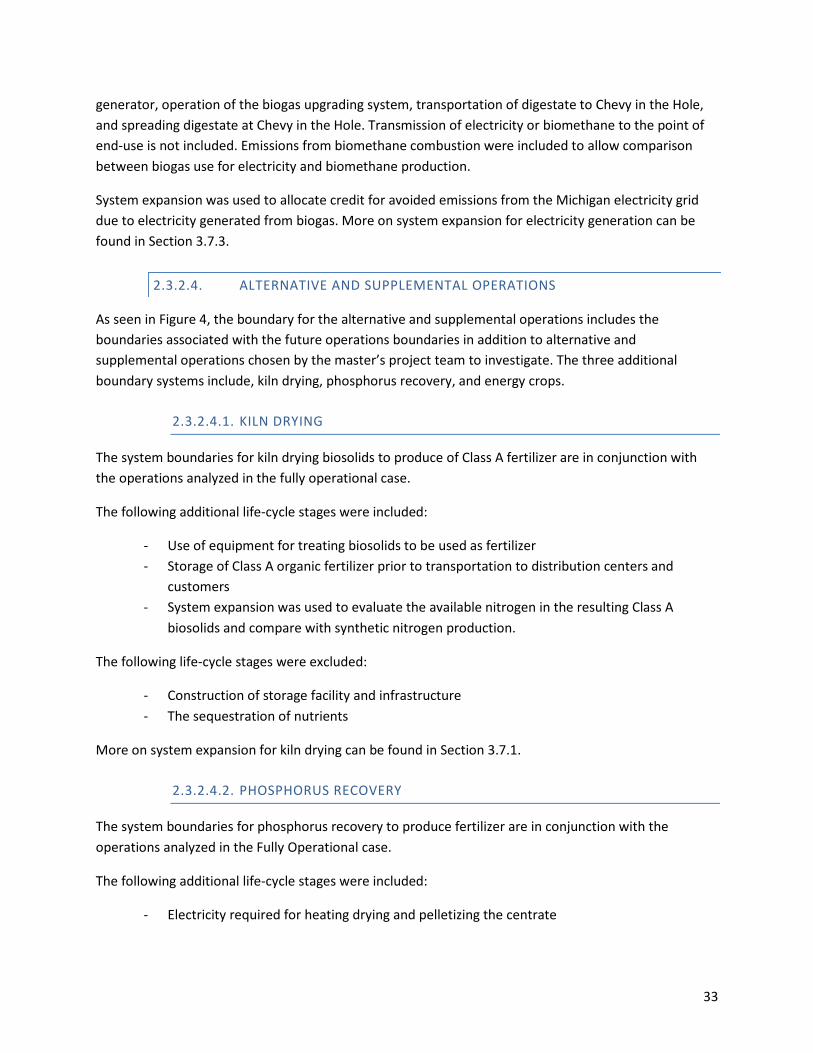
33
generator, operation of the biogas upgrading system, transportation of digestate to Chevy in the Hole, and spreading digestate at Chevy in the Hole. Transmission of electricity or biomethane to the point of end-use is not included. Emissions from biomethane combustion were included to allow comparison between biogas use for electricity and biomethane production.
System expansion was used to allocate credit for avoided emissions from the Michigan electricity grid due to electricity generated from biogas. More on system expansion for electricity generation can be found in Section 3.7.3.
2.3.2.4. ALTERNATIVE AND SUPPLEMENTAL OPERATIONS
As seen in Figure 4, the boundary for the alternative and supplemental operations includes the boundaries associated with the future operations boundaries in addition to alternative and supplemental operations chosen by the master’s project team to investigate. The three additional boundary systems include, kiln drying, phosphorus recovery, and energy crops.
2.3.2.4.1. KILN DRYING
The system boundaries for kiln drying biosolids to produce of Class A fertilizer are in conjunction with the operations analyzed in the fully operational case.
The following additional life-cycle stages were included:
- Use of equipment for treating biosolids to be used as fertilizer - Storage of Class A organic fertilizer prior to transportation to distribution centers and
customers - System expansion was used to evaluate the available nitrogen in the resulting Class A
biosolids and compare with synthetic nitrogen production.
The following life-cycle stages were excluded:
- Construction of storage facility and infrastructure - The sequestration of nutrients
More on system expansion for kiln drying can be found in Section 3.7.1.
2.3.2.4.2. PHOSPHORUS RECOVERY
The system boundaries for phosphorus recovery to produce fertilizer are in conjunction with the operations analyzed in the Fully Operational case.
The following additional life-cycle stages were included:
- Electricity required for heating drying and pelletizing the centrate

34
- System expansion of available phosphorus in fertilizer product offsetting the same amount of phosphorus being produced from mining.
The following life-cycle stages of were excluded:
- Transportation of product away from the SBI plant - Construction of nutrient recovery system - The reduced loading impact on the Flint wastewater treatment facility
More on system expansion for phosphorus recovery can be found in Section 3.7.2.
2.3.2.4.3. ENERGY CROPS
The system boundaries for growing maize at CitH are in conjunction with the operations analyzed in the Fully Operational case.
The following life cycle stages were included:
- Production of maize at CitH - Transportation of maize to the biogas plant - Processing of additional input at the plant
The following are life cycle stages were excluded:
- Material acquisition, construction, and transportation to SBI of the buildings, vehicles, and equipment used in maize production
- The ensiling process
No land change at CitH was accounted for in this analysis since the area was deforested prior to the temporal boundaries of the cases analyzed.
2.3.3. ALLOCATION METHODS
All impacts within the system boundaries are allocated to the biogas produced by the system. In addition we used system expansion to account for the emissions avoided from the reduction in fossil fuels combusted to generate electricity for the Michigan grid and the emissions avoided in the kiln drying and phosphorus recovery scenarios by reducing the amount of synthetic fertilizer production.
2.3.3.1. SYSTEM EXPANSION
Using system expansion involves taking the amount of environmental burdens and material inputs to produce the outputs that are not used within the product system and then subtracting environmental burdens and material inputs using the process that only produces these materials. For the purposes of this study we established the environmental benefit of biogas byproducts by the nutrients recovered or returned to the ecosystem. The analysis conducted in this study used system expansion in the kiln drying

35
and the phosphorus recovery scenarios as well as for electricity generated to evaluate the environmental benefits of each process. Details on the methodology used for system expansion in the kiln drying and phosphorus recovery scenarios and for electricity generation is found in Section 3.7.
2.3.4. DATA REQUIREMENTS
Much of the data for the Base Case LCA and current operations LCA are measurements or estimations based on operations at the Flint Wastewater Treatment Plant. Data for Base Case were from 2009-2011, and data for current operations were from June 2011 through February 2012. Although it would be ideal to have at least one entire year of data for the current operations LCA in order to account for seasonal variations, time constraints on the project made that impossible. We assume that the data averages would not change much as the time range for the data we do have includes the two most extreme seasons, summer and winter. Data for the LCAs in which we investigate potential impacts from different scenarios for future operations are estimates based on current operations, literature, and equipment specifications indicated by SBI’s Director of Operations to be representative of equipment that will be used in future operations. We used data specific to the United States from literature when available. However, in some cases the data was European, as many studies on anaerobic digestion have been conducted in Germany, Austria, and Sweden.
2.3.5. IMPACT METHODS
We assessed environmental impact based on three U.S. EPA TRACI midpoint impact categories. These impact categories are global warming potential, acidification potential, and smog formation potential. While we expect eutrophication potential to be an important impact of this system, we did not model this impact category. We expect that much of the nitrogen and phosphorus emissions would occur from land application of digestate. Modeling the eutrophication potential from these non-point sources was not possible due to time and data limitations.
2.4. SOFTWARE INTERFACE
The model was designed and built using Microsoft Excel as the primary user interface. This was chosen because of the universal application of Excel and the ability to utilize macros to carry out complex adjustments.
The model consists of 20 calculation worksheets corresponding to each of the major processes involved in biogas production and alternative scenarios. The primary user interface is through a dashboard located at the head of the file. See Figure 5 below.

36
Figure 5: Dashboard
The model dashboard allows the user to interface with the various systems associated with biogas production. The four buttons on the left of the dashboard allow the user to switch between the scenarios analyzed as part of the life cycle research. The rows located at the top of the dashboard allow the user to adjust the various inputs and allocations according to the active scenario, which is indicated at the top of the dashboard. The remainder of the dashboard reports information on the active biogas system. Cell color description is provided in Table 1.
Table 1: Cell Color Description
User input values Output indicator values Error or attention needed Sludge input adjustment
From the dashboard the user can select the four scenarios utilized in the model, Base Case, Current Operations, Fully Operational and Alternative and Supplemental Operations. Depending on the case selected, the “Input,” “Biogas Allocation,” “Digestate Allocation” and “Centrate Allocation” cells will become active or inactive. For example, selecting “Base Case” will disable the ability to adjust biogas, digestate and centrate allocations; selecting “Alternative and Supplemental Operations” will allow for all inputs to be customizable using drop down menus to select “Yes” or “No” for each input and allocation.
Various output indicators are provided for the MCF/hr being produced, Biogas Allocation and the percent solids entering the digester. These allow the user to identify the performance of the biogas system and make adjustments to calibrate the system to the actual conditions experienced at the facility.
Below the dashboard are output graphs to illustrate the energy, emissions, and impact assessment associated with the current system. The results for the various model simulations are explained further in the results section (Section 4) of this paper.

37
3. METHODOLOGY
This section outlines the methods, processes, research and evaluation techniques used to develop the Swedish Biogas International Environmental Impact Assessment Model. Topic areas involved with the modeling process are also reviewed including; biogenic carbon emissions, EPA regulations of biosolids management, and the multi-criteria decision analysis process used to evaluate the plausibility of future research projects.
3.1. MULTI-CRITERIA DECISION ANALYSIS
This study aims to develop an LCA model of current and projected future operations as defined by SBI. Other options for the use of the products and byproducts of anaerobic digestion that SBI could implement were explored as well. Given the myriad of biogas use, digestate disposal or value-added alternatives that exist, and limited resources to investigate all available options, multi-criteria decision analysis (MCDA) was employed to help narrow down and identify the most valuable areas of research.
3.1.1. INTRODUCTION TO MCDA
Multi-criteria decision analysis is an analytical tool for use in decision-making processes in which there are multiple, often conflicting, objectives. The general methodology for a MCDA process is outlined below.18
• Define the problem and objectives • Identify options for achieving the objectives • Identify the stakeholder(s) making the decision • Select an appropriate process to evaluate the alternatives
- Identify criteria to compare the options - Develop importance weights for criteria
• Make a decision
In this study, MCDA was used to investigate the options for SBI’s operations that would feasibly maximize profit, minimize environmental impact, and create social benefits. The decision-makers were the CEO and Director of Operations at SBI as well as the master’s project team.
3.1.2. APPLICATIONS FOR DIGESTATE
After reviewing literature on current applications of anaerobic digestion products and byproducts, we created a list of options to consider in the MCDA (see Table 2). Land application of digestate in Chevy in the Hole (CitH) was used as the baseline since it is the current course of action planned by SBI.
18 Comunities and Local Government. “Multi-criteria analysis: a manual.” Communities and Local Government Publications. 28 Jan. 2009. Web 17 Mar. 2012. <http:// eprints.lse.ac.uk/12761/1/Multi-criteria_Analysis.pdf>.

38
Table 2: Application of Anaerobic Digestion Products
Application of Anaerobic Digestion Products Description
Processes in conjunction with land application of biosolids in CitH
Pasteurization of Centrate Centrate is channeled through the heat exchanger of the CHP to be pasteurized, transported and land applied
Energy crops management Growing corn ethanol plants in CitH for the purpose of being used as a feedstock for the digesters
Phosphorus Nutrient Recovery from Centrate
Installing a nutrient recovery system to remove phosphorus from the dewatering of biosolids
Land Application of Class B Centrate
Centrate is collected from the centrifuge and transported to appropriate sites where it is applied as a Class B liquid fertilizer
Hydroponics Waste heat, CO2, and centrate are used to develop a hydroponics facility near the biogas plant
Urban Forestry Program for Greenhouse Gas Offset in CitH
Engaging with a forestry program to plant trees in CitH to absorb CO2 and bioremediation project
Capture of Waste CO2 for use in Greenhouse
Partner with the botany department at Kettering University to establish a greenhouse project to utilize waste CO2 from the SBI facility
Processes alternative to land application of biosolids in CitH
Class A/B: Urban Agriculture Program
Establishing an Urban Agriculture program where biosolids are utilized as a Class B fertilizer
Class A: Upgrading of biosolids using kiln drying
Using a kiln drier, heated by biogas to upgrade biosolids to Class A certification and to be sold as a fertilizer product
Class A: Upgrading of biosolids through outdoor composting
Using a kiln drier, heated by biogas to upgrade biosolids to Class A certification and to be sold as a fertilizer product
Class A: Two-stage thermophilic digestion to pasteurize biosolids
Using higher temperatures for digestion and for longer retention time to pasteurize the biosolids to meet Class A regulations.
Class B: Farm and forest application of biosolids
Applying the biosolids on local fields or forests as a soil amendment
Class B: Locating additional Superfund sites for land application
Identifying and applying other Superfund sites near Flint, Michigan for application of biosolids
Class B: Biosolids Amendment for Coal
Using the biosolids as an amendment for coal to be used in local coal plants as a fuel supplement

39
3.1.3. CRITERIA
The criteria used to evaluate the options were factors predicted to affect SBI’s development as a company, relevant to SBI’s mission and in compliance with applicable regulations. These factors address the triple bottom line: economics, society, and the environment. Additionally, the feasibility of the options based on current and predicted future conditions were evaluated. A list of all criteria can be found in Table 3.
Table 3: Criteria Used to Evaluate Options for Digestate Application
Social Environmental Job Creation in Flint Reducing GHG Emissions Disposal Aesthetics to Public Reducing Water Pollution Company Image to All Stakeholders Reducing Negative Land Use Company Exposure to Flint Community Reducing Ecotoxicity Education Opportunities in Flint Community Preserving Biodiversity Crime Reduction in Flint Community Reducing Acid Rain Recreation in Flint
Economic Practicality Initial Investment Technical Feasibility O&M Political Feasibility (regulations) Payback Period Resiliency to Market Changes Profit
3.1.4. EVALUATION TECHNIQUE
To evaluate the values of these options, we employed a utility and weighting method. This involved assigning weights to each of the criteria based on their importance, assigning scores for the criteria for each option, and then taking a weighted average to determine a one score for each option so that the options could be compared to each other.
The weights assigned to each option were on a scale of 1 to 5, 1 being a factor of mild importance and 5 being a factor that is of highest importance. The weights assigned to the criteria were an average of values given by the decision makers listed above in a survey. A table of all the weights can be found in Appendix 1.
Scores for each criterion were based on their utility relative to the reference option, land application of digestate at Chevy in the Hole. Scores were based on a scale of 1, 2, and 3. Scores of 2 were defined as operations that have impact equal to land application of digestate at CitH. Scores of 1 and 3 were defined as relative negative or positive effects the options would have respective to the reference. The scores were determined based on a survey generated by the master’s project team. Addressing the substantial level of subjectivity in assigning scores, the survey was conducted three separate times, blind to previous answers.

40
To calculate the final scores a weighted average was used of the weights and scores for each criteria and option:
𝑆𝑖 = �𝑤𝑖𝑠𝑖𝑗
𝑛
𝑗=1
S = total score for each option w = weight of each criterion sij = score for option i on criterion j
The score was then averaged across the results of the three trial surveys to determine a final score for each option.
3.1.5. MCDA RESULTS
A table displaying the results of the master’s project team’s surveys to score each criterion is found in Appendix 1. Based on our three surveys, the standard deviation of the total scores for each option ranged from 1.15 to 8.32.
Final scores for all options are shown in The three highest ranking options were quite similar, so the master’s project team chose to look at the highest ranking option of the three - growing energy crops at Chevy in the Hole. The team then chose the highest ranking option that utilized a different byproduct of anaerobic digestion and could be done in conjunction with CitH or independently – phosphorus recovery from the centrate. Finally, the team chose the highest ranking option that was an alternative to Chevy in the Hole – Kiln drying biosolids to make compost.
The results can be seen in Figure 6 broken down by each option’s score in the practicality, environmental, social, and economic criteria categories. The MCDA identified four options that were more beneficial than land application of digestate at CitH, all of which would be implemented in conjunction with Chevy in the Hole: growing energy crops at CitH, using CitH for urban agriculture, growing trees at CitH to sequester greenhouse gases, and using the phosphorous from centrate for land application. We discuss some of these options in greater detail in Section 5.
The three highest ranking options were quite similar, so the master’s project team chose to look at the highest ranking option of the three - growing energy crops at Chevy in the Hole. The team then chose the highest ranking option that utilized a different byproduct of anaerobic digestion and could be done in conjunction with CitH or independently – phosphorus recovery from the centrate. Finally, the team chose the highest ranking option that was an alternative to Chevy in the Hole – Kiln drying biosolids to make compost.
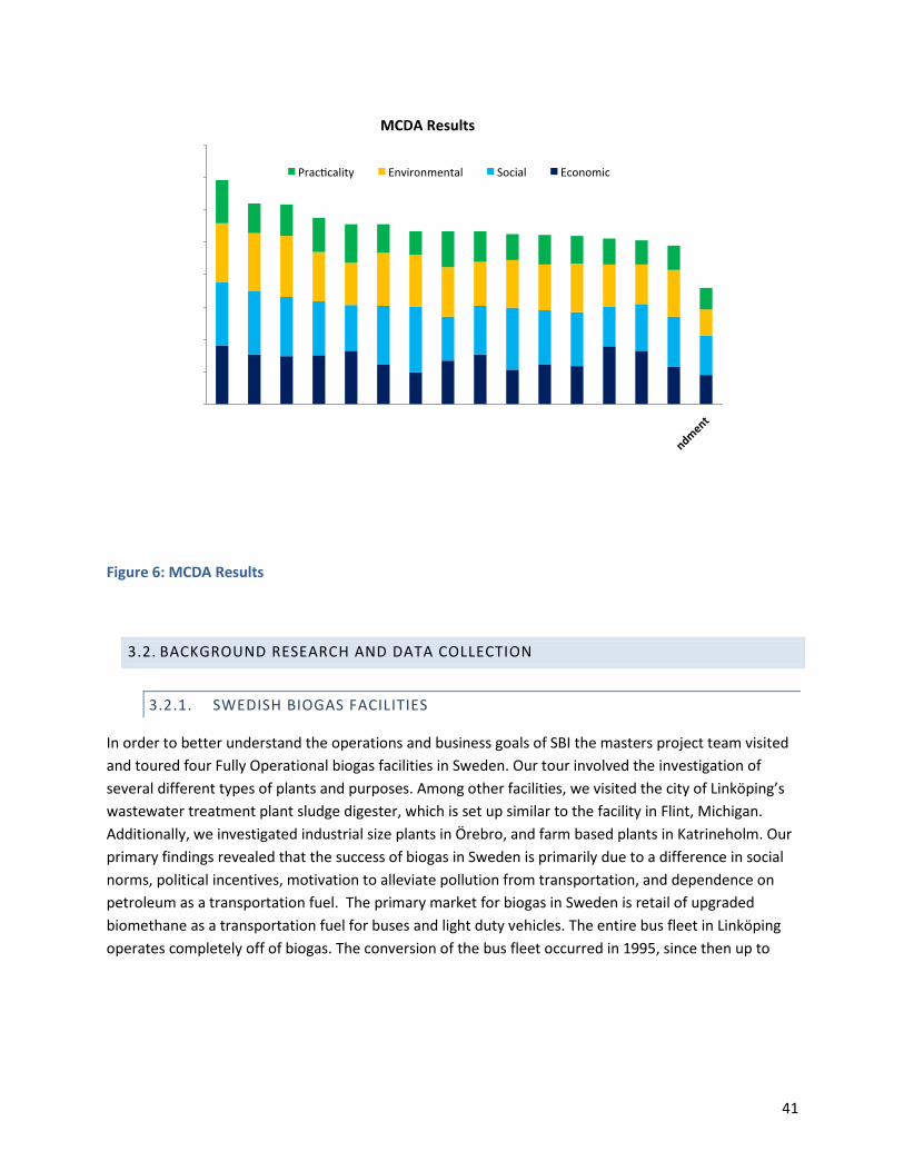
41
Figure 6: MCDA Results
3.2. BACKGROUND RESEARCH AND DATA COLLECTION
3.2.1. SWEDISH BIOGAS FACILITIES
In order to better understand the operations and business goals of SBI the masters project team visited and toured four Fully Operational biogas facilities in Sweden. Our tour involved the investigation of several different types of plants and purposes. Among other facilities, we visited the city of Linköping’s wastewater treatment plant sludge digester, which is set up similar to the facility in Flint, Michigan. Additionally, we investigated industrial size plants in Örebro, and farm based plants in Katrineholm. Our primary findings revealed that the success of biogas in Sweden is primarily due to a difference in social norms, political incentives, motivation to alleviate pollution from transportation, and dependence on petroleum as a transportation fuel. The primary market for biogas in Sweden is retail of upgraded biomethane as a transportation fuel for buses and light duty vehicles. The entire bus fleet in Linköping operates completely off of biogas. The conversion of the bus fleet occurred in 1995, since then up to

42
seven percent of the city’s vehicle fuel has come from biogas and there is significant reduction in city pollution due to decreased diesel emissions.19
In addition to understanding the cultural motivations and primary business drivers behind the SBI business model, we were able to establish valuable working relationships with the Swedish counterparts at SBI. This relationship allowed for information sharing and insight into Fully Operational biogas systems. We also established partnerships at the academic institution of Linköping University. This allowed for greater access to knowledge within the research conducted in Sweden on the application of biosolids as fertilizer, biogas production and use as a transportation fuel.
3.2.2. AIR EMISSIONS
Quantifying air emissions from the Flint facility was an essential element of the project and research goals. Collecting and measuring primary air emissions data from the Flint biogas plant was outside the scope of the project scope because of the challenges associated with collecting empirical data in the timeframe of the study. In order to calculate accurate air emission data emanating from the facility, historical monitoring data reported to the EPA, literature on emission sources and primary elemental analysis data was used. A breakdown of sources is provided below. See Appendix 2: Emission Factors for a full list of emissions factors.
BOILER EMISSIONS:
• GREET1_2011 Model20 • Literature21
FLARING EMISSIONS:
• GREET1_2011 Model • Literature22
INCINERATOR EMISSIONS:
• EPA Emission Factors from AQ-29 provided by City of Flint Wastewater Treatment Plant23
19 SBI. "Swedish Biogas International." History. Web. 15 Apr. 2012. <http://www.swedishbiogas.com/us/about-us/history>.
20 Argonne National Laboratory. “GREET1_2011 Model.” 2011. Web. < http://greet.es.anl.gov/>. 21 Electrigaz Technologies Inc. "Feasibility Study – Biogas Upgrading and Grid Injection in the Fraser Valley, British Columbia." Electrigaz. 2007. Web. <www.lifesciencesbc.ca/files/PDF/feasibility_study_biogas.pdf>.
22 Ibid.
43
• Elemental Analysis of Dewatered Cake from City of Flint Wastewater Treatment Plant24 • U.S. EPA Emission Factors from AP-4225
GENERATOR EMISSIONS:
• Generator Specifications • Literature26
BIOGAS UPGRADER EMISSIONS:
• Upgrader Specifications • eGRID Electricity Emission Factors for RFC Michigan27
PHOSPHORUS NUTRIENT RECOVERY EMISSIONS:
• Ostara Nutrient Recovery Technologies • eGRID Electricity Emission Factors for RFC Michigan
KILN DRYING EMISSIONS:
• GREET1_2011 Model from Argonne National Laboratory • eGRID Electricity Emission Factors for RFC Michigan • Literature28
23 City of Flint Wastewater Treatment Plant. "Annual Report to Michigan Department of Environmental Quality on City of Flint Wastewater Treatment Plant Air Emissions." (2011). Print.
24 City of Flint Wastewater Treatment Plant. “Calorific Value and Elemental Analysis of the City of Flint WPCD Sludge Cake.” (2011). Print.
25 US EPA. “AP-42: Natural Gas Combustion.” 1998. Web. <http://www.epa.gov/ttnchie1/ap42/ch01/final/c01s04.pdf>.
26 Nielsen, M., and J. B. Illerup. "Danish Emission Inventories for Stationary Combustion Plants, Inventories until Year 2001." National Environmental Research Institute192nd ser. (2003). Print.
27 U.S. Environmental Protection Agency. “eGRID2010 Version 1.1 Year 2007 GHG Annual Output Emission Rates.” 2010. Web. <http://www.epa.gov/cleanenergy/energy-resources/egrid/index.html#download>.
28 Electrigaz Technologies Inc. 2007. “Feasibility Study – Biogas upgrading and grid injection in the Fraser Valley, British Columbia.” Prepared for the BC Innovation Council.

44
3.2.3. BIOSOLIDS MANAGEMENT AND EPA REGULATIONS
In order to better understand the opportunities of biosolids management we conducted research onthe regulations and best practices for biosolids disposal. Our research showed that the anaerobic digestion process removes nearly all pathogens from sewage sludge biosolids; however, adverse health effects may result from contact with the small remaining constituency of pathogens. Additionally, the constituency of organic material is attractive to vectors under certain conditions. Therefore, the use and disposal of anaerobically digested biosolids are strictly regulated. To ensure compliance with federal and state laws for our recommendations, Environmental Protection Agency (EPA) and Michigan Department of Environmental Quality (MDEQ) regulations were investigated and compared to previous, current and future operations respectively. Michigan does not have county-wide regulations, though some townships have local ordinances. None is applicable to Flint.29
Acceptable federal sewage sludge biosolids use and disposal methods are outlined in EPA 503 Regulations. The 503 Rule encompasses use or disposal, land application, surface disposal, incineration, pathogen and vector attraction reduction, and permit application for biosolids.30
The principal source for state laws used was MDEQ’s Biosolids Program website. A law specific to Michigan is Act 29, which amended the Natural Resources and Environmental Protection Act (NREPA). It describes state-specific application of biosolids.31 The MDEQ website was also referenced to determine what incentives are available for applying biosolids. The MDEQ encourages biosolids application to agriculture and silviculture.32
3.3. MODELING THE BASE CASE
Modeling the Base Case consisted of calculating the electricity use for dewatering and incineration equipment, estimating the sludge input to the incinerator, and finding the natural gas use and incineration emissions for an average of 9 dry tons of sludge input per day.
29 Zamani, Bahram. Head of Michigan Biosolids Management Program for Genessee County and Middle Michigan, Michigan Department of Environmental Protection. Personal phone communication. 2011.
30 http://water.epa.gov/scitech/wastetech/biosolids/503pe_index.cfm
31 http://www.michigan.gov/deq/0,4561,7-135-3313_3683_3720-9615--,00.html
32 http://www.michigan.gov/deq/0,1607,7-135-3313_3683_3720---,00.html

45
Electricity consumption for 2 pumps, the grinder, the belt filter press and incinerator equipment was calculated by multiplying recorded power ratings (kW) by weekly run times to get kWh per week, then divided by 7 to find kWh per day. 33
In the dewatering step, the belt filter press dewatered the sludge to approximately 23% TS.34 A solids capture rate of 95% was used to model how much of the biosolids continued to the incineration stage and how much were returned to the wastewater treatment plant in the centrate.35 Polymer use was modeled based on an average use of 6 pounds of 100% active polymer per dry ton of sludge.36 Dry tons of output to the incinerator, kiln-dryer, or land application was found by multiplying the dry tons of digestate input by the 95% capture rate. The amount of water returned to the head of the plant as centrate was calculated by subtracting the water content of the resulting cake from the water content of the sludge input to the belt filter press.
For incineration, natural gas use was computed by multiplying the dry weight of input to incineration (8.55 dry tons/day after dewatering) by the natural gas use per dry ton of incinerator input factor. Air emissions from biosolids combustion were calculated by multiplying the dry weight input to incineration by the emissions factors for biosolids combustion. Air emissions from natural gas combustion were calculated by multiplying the total natural gas usage per year by the emissions factors for natural gas combustion. See Section 3.5.1 for more information on modeling natural gas use and emissions from incineration.
3.4. MODELING THE BIOGAS PRODUCTION PROCESS
SBI received sludge in the form of primary sludge and skimmings stored in the East tank. Averages of November 2011 through February 2012 data showed that daily primary sludge inputs to the digester were about 33,000 gallons, or 7.6 dry tons, with approximately 5.5% total solids (TS), of which 63% were volatile solids (VS). 37 Average daily skimmings input directly to the digester were about 6,000 gallons, or
33 SBI-PESA 2012 rev 2.xlsx; Electrical Energy Tracking Worksheet
34 City of Flint Wastewater Treatment Plant. 2011. “Calorific Value and Elemental Analysis of the City of Flint WPCD Sludge Cake.”
35 SBI. 2010. “Biogas Design Upgrade Summary”
36 Chad Antle. Personal communication. 23 September 2011. 37 Antle, Chad. SBI-PESA 2012 Rev 2; Loading Worksheet. 2012.
46
0.7 dry tons, with approximately 2.9% TS and 55% VS. 38 Also, approximately 1,250 gallons or 0.3 dry of thickened skimmings with 5.4% TS and 61%VS were added to the digester each day. 39
Food waste from vendors was included as an input to the digester in the Fully Operational case. We assumed, based on conversations with SBI’s process engineer, that food waste input would have an average of 12.5% TS and 80% VS of TS.40
3.4.1. TRANSPORTATION OF FOOD WASTE
Using data that estimated potential sources, locations and volumes of food waste, we created a table that calculated the distance from each food waste source and emissions associated with transportation to SBI.41 At the time we wrote this paper, we did not have information regarding which source(s) SBI would use as input in future operations. Therefore, we created a table of default data, which averaged the average volume a truck could transport (5000 gallons) and distance from all potential locations (114 miles). Assuming that the trucks run on diesel fuel and a fuel economy of 6 miles per gallon of diesel fuel, we calculated potential emissions. Additionally, we used the user defined food waste input value to calculate the average number of incoming trucks per week and the average volume of food waste per day, week, and year.
3.4.2. SLUDGE THICKENING
The maximum daily volume of input to the digester was determined by dividing the volume of the tanks in use by the appropriate hydraulic retention time (HRT). We assumed an HRT of 20 days for sludge only and 30 days if food waste or energy crops were included. Thus, the maximum daily input was 47,000 gallons for sludge and 31,333 gallons for sludge and food waste or energy crops.42 As the initial volume of primary sludge, skimmings, or food waste input to the system increased, the more material that had to pass through the gravity belt thickener (GBT) in order to remove water and maintain the maximum input volume. The amount of water returned to the head of the plant as centrate was calculated by subtracting the water content of the thickened materials from the water content of the process input.
In the model, the amount of primary sludge, skimmings, food waste, or energy crops sent through the thickening process was determined by user input. The %TS of the output from the GBT was also user defined. However, we used a default rate of 7% TS output for primary sludge, food waste, or energy
38 Ibid.
39 Ibid.
40 Brynas, Anna. Personal e-mail communication. 29 March 2012.
41 Antle, Chad. Personal e-mail communication. 2011.
42 Antle, Chad. Personal phone communication. 23 March 2012.

47
crops input and 5% TS output for sludge skimmings input.43 44 A solids capture rate of 95% was used to model how much of the biosolids continued to the digestion stage and how much were returned to the wastewater treatment plant in the centrate.45 Polymer use was modeled based on an average use of 6 pounds of 100% active polymer per dry ton of sludge.46
The amount of sludge processed by the GBT was limited by the maximum solids loading rate of 1,651 pounds per hour and the maximum hydraulic loading rate of 110 gallons per minute.47 The run time of the GBT and associated equipment was based on the number of hours per day necessary to process the total daily input to the thickening process. Since the run time necessary to handle the hydraulic loading would be different from the run time needed to handle the solids loading, the run time of the GBT was taken to be the greater of the two.
Another major input to this stage was the electricity to run the pumps and thickening equipment. Modeling of electricity used by equipment in sludge thickening is discussed in Section 3.4.6.
3.4.3. DIGESTION
The digester tank must be continually heated to approximately 98°F.48 The heat may come from the boiler burning either biogas or natural gas or from the waste heat from the generator. To determine the energy needed to heat each digester, we calculated the average weekly use of natural gas in the boiler using data from January 7 to February 3, 2012.49 Since this value was calculated from winter months only, it was likely higher than a yearly average would be. However, it was the best available data at the time of the calculation. We also assumed that the amount of heat needed for each digester would remain constant as the volume of material would remain constant and that solids and water require approximately the same amount of energy to heat. Using a heating value of 1000 MBtu/MCF of natural gas, we estimated the digester needed 18,571 MBtu/day to maintain 100°F. This translated to an average of 1.17 MCF of biogas/hour required by the boiler to heat the digester. If there was not enough biogas, natural gas was used to meet the remaining energy needs.
43 Antle, Chad. Personal e-mail communication. 28 March 2012.
44 Antle, Chad. SBI-PESA 2012 Rev 2; Loading Worksheet. 2012.
45 Antle, Chad. SBI. “Biogas Design Upgrade Summary.” 2010.
46 Antle, Chad. SBI-PESA 2012 Rev 2; Weekly Summary Worksheet. 2012.
47 Antle, Chad. SBI. 2010. “Biogas Design Upgrade Summary.” 2012.
48 Antle, Chad. Personal communication. 26 May 2011.
49 Antle, Chad. SBI-PESA 2012 Rev 2; Natural Gas Worksheet. 2012.

48
Emissions from natural gas combustion, if any, were calculated by multiplying the amount of natural gas combusted each year by emissions factors for criteria pollutants and greenhouse gases derived from GREET1_2011 for a small industrial natural gas boiler.50
Emissions from the biogas combustion in the boiler were estimated by multiplying the amount of biogas combusted each year by emissions factors for criteria pollutants and greenhouse gases derived from literature and GREET1_2011 for a small industrial natural gas boiler.51, 52 All of the CO2 content in biogas was assumed to pass through the boiler and into the air as CO2. We also assumed that the total hydrogen sulfide (H2S) content of biogas was released as SO2. Stoichiometric calculations were used to convert the volume of CO2 and H2S per 1 MCF of biogas to pounds of CO2 and SO2 per 1 MCF of biogas. The resulting CO2 emissions factor was added to the CO2 emissions factor from the GREET1_2011 model. (See Appendix 2: Emission Factors for a table of emission factors for biogas combustion in the boiler.)
If the generator was operating, the waste heat from the generator was used to heat the digester 97% of the year.53 If there was not enough heat from the CHP, natural gas was used to meet the remaining energy requirements of the digester. For the remaining 3% of the year, biogas was used to heat the digester to account for scheduled maintenance of the generator.54 Calculations for emissions from the generator are discussed in Section 3.6.2.
The production of biogas was modeled based on calculations of tons of volatile solids (VS) per dry ton of input and methane production potentials. Using current measurements of %VS of TS (66%, 80%, and 24.2% for sludge, food waste, and energy crops, respectively),55 ,56, 57 we calculated the amount of volatile solids for the amount of dry tons of sludge and food waste input per day. We multiplied the results by the methane production potentials of 9,600 cubic feet (cf) of methane (CH4) per ton of VS in sludge, 14,000 cf of CH4 / 1 ton VS in food waste, and 3,108 cf of CH4 / 1 ton VS.58,59 Using a
50 Argonne National Laboratory. “GREET1_2011 Model.” 2011. Web. < http://greet.es.anl.gov/>.
51 Electrigaz Technologies Inc. "Feasibility Study – Biogas Upgrading and Grid Injection in the Fraser Valley, British Columbia." Electrigaz. 2007. Web. <www.lifesciencesbc.ca/files/PDF/feasibility_study_biogas.pdf>.
52 Argonne National Laboratory. “GREET1_2011 Model.” 2011. Web. < http://greet.es.anl.gov/>.
53 Antle, Chad. Personal e-mail communication. 13 September 2011.
54 Antle, Chad. Personal e-mail communication. 13 September 2011.
55 Antle, Chad. SBI-PESA 2012 Rev 2; Weekly Summary Worksheet. 2012.
56 Brynas, Anna. Personal e-mail communication. 29 March 2012.
57 Nges, Ivo, Frederico Escobar, and Lovisa Bjornsson. "Benefits of Supplementing Industrial Waste Anaerobic Digestion for Increased Biogas Production." Science Direct. Waste Management, Mar. 2011. Web. <http://www.sciencedirect.com/science/article/pii/S0956053X11003904>.
58 Brynas, Anna. Personal e-mail communication. 29 March 2012.
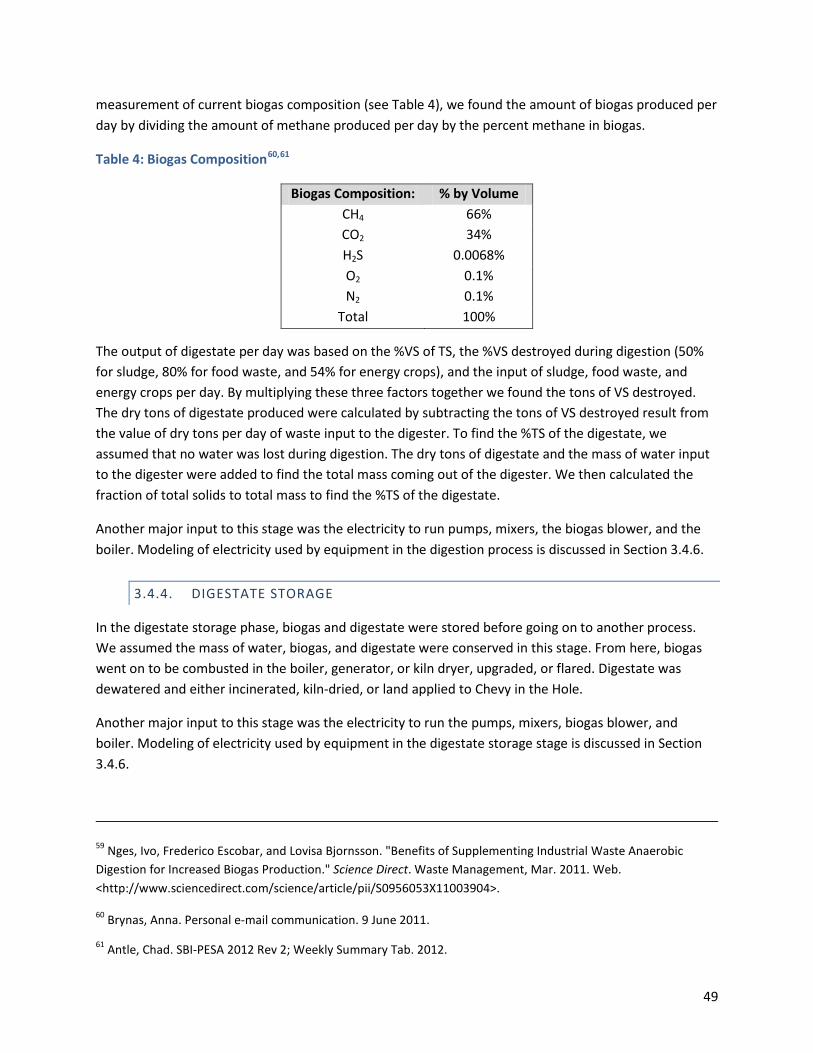
49
measurement of current biogas composition (see Table 4), we found the amount of biogas produced per day by dividing the amount of methane produced per day by the percent methane in biogas.
Table 4: Biogas Composition60,61
Biogas Composition: % by Volume CH4 66% CO2 34% H2S 0.0068% O2 0.1% N2 0.1%
Total 100%
The output of digestate per day was based on the %VS of TS, the %VS destroyed during digestion (50% for sludge, 80% for food waste, and 54% for energy crops), and the input of sludge, food waste, and energy crops per day. By multiplying these three factors together we found the tons of VS destroyed. The dry tons of digestate produced were calculated by subtracting the tons of VS destroyed result from the value of dry tons per day of waste input to the digester. To find the %TS of the digestate, we assumed that no water was lost during digestion. The dry tons of digestate and the mass of water input to the digester were added to find the total mass coming out of the digester. We then calculated the fraction of total solids to total mass to find the %TS of the digestate.
Another major input to this stage was the electricity to run pumps, mixers, the biogas blower, and the boiler. Modeling of electricity used by equipment in the digestion process is discussed in Section 3.4.6.
3.4.4. DIGESTATE STORAGE
In the digestate storage phase, biogas and digestate were stored before going on to another process. We assumed the mass of water, biogas, and digestate were conserved in this stage. From here, biogas went on to be combusted in the boiler, generator, or kiln dryer, upgraded, or flared. Digestate was dewatered and either incinerated, kiln-dried, or land applied to Chevy in the Hole.
Another major input to this stage was the electricity to run the pumps, mixers, biogas blower, and boiler. Modeling of electricity used by equipment in the digestate storage stage is discussed in Section 3.4.6.
59 Nges, Ivo, Frederico Escobar, and Lovisa Bjornsson. "Benefits of Supplementing Industrial Waste Anaerobic Digestion for Increased Biogas Production." Science Direct. Waste Management, Mar. 2011. Web. <http://www.sciencedirect.com/science/article/pii/S0956053X11003904>.
60 Brynas, Anna. Personal e-mail communication. 9 June 2011.
61 Antle, Chad. SBI-PESA 2012 Rev 2; Weekly Summary Tab. 2012.
50
3.4.5. DEWATERING
In the dewatering step, centrifuges dewatered the digestate to approximately 26% TS.62 A solids capture rate of 95% was used to model how much of the biosolids continued to the next stage and how much were returned to the wastewater treatment plant in the centrate.63 Polymer use was modeled based on an average use of 11.4 pounds of 100% active polymer per dry ton of sludge.64 Output (dry tons/day) to the incinerator, kiln-dryer, or land application was found by multiplying the dry tons of digestate input by the 95% capture rate. The amount of water returned to the head of the plant as centrate was calculated by subtracting the water content of the resulting cake from the water content of the incoming digestate.
Modeling of electricity used by the centrifuges is discussed in Section 3.4.6.
3.4.6. ELECTRICITY USE
Reported electricity use data were used to make regression models that estimated the amount of electricity consumed by each piece of equipment per dry ton of input per day (kWh/dt/day).65
CURRENT OPERATIONS Electricity consumption for sludge thickening equipment was calculated by multiplying kW by the GBT run time (hours/day) value measured in the sludge thickening worksheet. These values were calculated based on the number of hours the GBT is running since previously recorded data from plant operations to date are not measured on a time scale narrow enough to determine when the GBT was running in relation to incoming sludge. To calculate electricity consumption for all other equipment in the current operations case used we referred to recorded data. To determine the relationship between accumulated tons of input (x-axis) and elapsed kWh (y-axis) for a given time period we graphed scatter plots for each piece of equipment. Each time period spanned approximately two-months, the dates of which were based on a period steady use for each piece of equipment. We then added the regression trend line with the highest R-squared value each graph. Best-fit trend line equations were then used to calculate the kWh for a given number of dry tons: Trend line Equation Linear 𝑦 = 𝑚𝑥 + 𝑏 Polynomial 𝑦 = 𝑎𝑥2 + 𝑏𝑥 + 𝑐
62 Antle, Chad. Personal communication. 26 May 2011.
63 Antle, Chad. SBI. “Biogas Design Upgrade Summary.” 2010.
64 Antle, Chad. SBI-PESA 2012 Rev 2; Weekly Summary Tab. 2012.
65 Antle, Chad. SBI-PESA 2012 rev 1.xlsx. 2012.
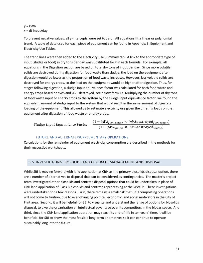
51
y = kWh x = dt input/day
To prevent negative values, all y-intercepts were set to zero. All equations fit a linear or polynomial trend. A table of data used for each piece of equipment can be found in Appendix 3: Equipment and Electricity Use Tables.
The trend lines were then added to the Electricity Use Summary tab. A link to the appropriate type of input (sludge or food) in dry tons per day was substituted for x in each formula. For example, all equations in the Digestion section are based on total dry tons of input per day. Since more volatile solids are destroyed during digestion for food waste than sludge, the load on the equipment after digestion would be lower as the proportion of food waste increases. However, less volatile solids are destroyed for energy crops, so the load on the equipment would be higher after digestion. Thus, for stages following digestion, a sludge input equivalence factor was calculated for both food waste and energy crops based on %VS and %VS destroyed, see below formula. Multiplying the number of dry tons of food waste input or energy crops to the system by the sludge input equivalence factor, we found the equivalent amount of sludge input to the system that would result in the same amount of digestate loading of the equipment. This allowed us to estimate electricity use given the differing loads on the equipment after digestion of food waste or energy crops.
𝑆𝑙𝑢𝑑𝑔𝑒 𝐼𝑛𝑝𝑢𝑡 𝐸𝑞𝑢𝑖𝑣𝑎𝑙𝑒𝑛𝑐𝑒 𝐹𝑎𝑐𝑡𝑜𝑟 =(1 − %𝑉𝑆𝑓𝑜𝑜𝑑 𝑤𝑎𝑠𝑡𝑒 × %𝑉𝑆𝑑𝑒𝑠𝑡𝑟𝑜𝑦𝑒𝑑𝑓𝑜𝑜𝑑 𝑤𝑎𝑠𝑡𝑒)
(1 − %𝑉𝑆𝑠𝑙𝑢𝑑𝑔𝑒 × %𝑉𝑆𝑑𝑒𝑠𝑡𝑟𝑜𝑦𝑒𝑑𝑠𝑙𝑢𝑑𝑔𝑒)
FUTURE AND ALTERNATE/SUPPLEMENTARY OPERATIONS Calculations for the remainder of equipment electricity consumption are described in the methods for their respective worksheets.
3.5. INVESTIGATING BIOSOLIDS AND CENTRATE MANAGEMENT AND DISPOSAL
While SBI is moving forward with land application at CitH as the primary biosolids disposal option, there are a number of alternatives to disposal that can be considered as contingencies. The master’s project team investigated other biosolids and centrate disposal options that could be undertaken in place of CitH land application of Class B biosolids and centrate reprocessing at the WWTP. These investigations were undertaken for a few reasons. First, there remains a small risk that CitH composting operations will not come to fruition, due to ever-changing political, economic, and social motivators in the City of Flint area. Second, it will be helpful for SBI to visualize and understand the range of options for biosolids disposal, to give the organization an intellectual advantage over its competitors in the biogas space. And third, since the CitH land application operation may reach its end-of-life in ten years’ time, it will be beneficial for SBI to know the most feasible long-term alternatives so it can continue to operate sustainably long into the future.

52
As biosolids are one of the main products of anaerobic digestion and produce a substantial amount of organic material that can be beneficially recycled, we have investigated several value-added applications.
Due to detectable levels of pathogens that remain in the biosolids after anaerobic digestion, properties that are attractive to the introduction and growth of new vectors, and pollutant concentrations, there are strict restrictions on management and disposal. These restrictions are part of the EPA 503 regulations. In this section we discuss four options for land application and centrate use. Land application is defined as “the application of biosolids to land to either condition the soil or fertilize crops or other vegetation grown in the soil.”66 Biosolids used for land application are categorized by their level of pathogenicity:
CLASS A:
Pathogens (e.g. Salmonella sp. Bacteria, enteric viruses, and viable helminth ova) are undetectable67
CLASS B:
Contains detectable levels of pathogens but are at levels that do not pose a threat to public health if certain precautions are taken to prevent exposure in use and disposal68
There are several methods to upgrade biosolids from Class B to Class A such as: thermal treatment through defined regimens, thermal and high pH treatment, composting, heat drying, thermophilic aerobic digestion, beta ray irradiation, gamma ray irradiation, and pasteurization. Methods not described in the EPA 503 regulations handbook can also be tested for pathogens to be classified as Class A.69
Given that treating biosolids for upgrading from Class B to Class A requires more time and money, the tradeoff is that Class A biosolids have a wider, less restrictive variety of applications.
66 U.S. EPA. "A Plain English Guide to the EPA Part 503 Biosolids Rule - Chapter 2." U.S. EPA. Web. 15 Apr. 2012. <http://water.epa.gov/scitech/wastetech/biosolids/503pe_index.cfm>.
67 U.S. EPA. "A Plain English Guide to the EPA Part 503 Biosolids Rule - Chapter 5." U.S. EPA. Web. 15 Apr. 2012. <http://water.epa.gov/scitech/wastetech/biosolids/503pe_index.cfm>.
68 U.S. EPA. "A Plain English Guide to the EPA Part 503 Biosolids Rule - Chapter 5." U.S. EPA. Web. 15 Apr. 2012. <http://water.epa.gov/scitech/wastetech/biosolids/503pe_index.cfm>.
69 U.S. EPA. "A Plain English Guide to the EPA Part 503 Biosolids Rule - Chapter 5." U.S. EPA. Web. 15 Apr. 2012. <http://water.epa.gov/scitech/wastetech/biosolids/503pe_index.cfm>.

53
3.5.1. INCINERATION
Historically, the City of Flint Wastewater Treatment Plant has incinerated their biosolids. Incineration is a relatively controlled method of biosolids disposal as the resulting emissions are from a point source and control devices can generally remove a large portion of the most offensive emissions.
ASSUMPTIONS:
• Zero nitrogen or carbon content in the ashes.70 • The moles of CO2 emissions from combustion of 1 ton of sludge was equal to the moles of carbon in
one ton of sludge after subtracting the moles of carbon that were released in the form of VOCs and carbon monoxide (CO).
• Zero methane emissions from combustion of the sludge as any CH4 present in the sludge would be combusted and converted into CO2.
• The moles of N2O emissions from combustion of 1 ton of sludge was equal to the moles of nitrogen in one ton of sludge after subtracting the moles of nitrogen that were released in the form of nitrogen oxides (NOx) where half of the NOx is NO and half is NO2.
ENVIRONMENTAL ANALYSIS:
Dry tons of solids input to incineration were taken from dewatering. A natural gas use per dry ton of incinerator input factor (MCF/dry tons of dewatered biosolids) was calculated by dividing the total volume of natural gas combusted in 2011 (MCF/yr) by the total incinerator inputs for 2011 (dry tons/yr).71 This factor was multiplied by the dry weight of input to incineration per day to find the daily and yearly natural gas consumption.
Emissions factors for both natural gas and biosolids combustion were taken from EPA Emission Factors from AQ-29 provided by City of Flint Wastewater Treatment Plant except for CO2, CH4, and N2O. 72 For natural gas combustion, these three factors were taken from US EPA AP-42 emission factors.73 For biosolids combustion, the total carbon and nitrogen content of 1 ton of dewatered solids were estimated using the Elemental Analysis of Dewatered Cake from City of Flint Wastewater Treatment Plant.74 Stoichiometric calculations were performed to find the moles of carbon remaining after release
70 Willems, M., B. Pedersen, and S. Storgaard Jørgensen. “Composition and Reactivity of Ash from Sewage Sludge.” Ambio. Vol. 5, No. 1 (1976), pp. 32-35. 71 City of Flint Wastewater Treatment Plant. “Annual Report to Michigan Department of Environmental Quality on City of Flint Wastewater Treatment Plant Air Emissions.” (2011). Print.
72 Ibid.
73 US EPA. “AP-42: Natural Gas Combustion.” 1998. Web. <http://www.epa.gov/ttnchie1/ap42/ch01/final/c01s04.pdf>.
74 City of Flint Wastewater Treatment Plant. “Calorific Value and Elemental Analysis of the City of Flint WPCD Sludge Cake.” (2011). Print.

54
of carbon monoxide and VOCs. We assumed the remaining moles of carbon were emitted as CO2 since the amount of CH4 was likely to be very low due to the relatively high temperature of combustion in the incinerator. Stoichiometric calculations were performed to find the moles of nitrogen remaining after release of NOx. We assumed the remaining moles of nitrogen were emitted as N2O.
Air emissions from biosolids combustion were calculated by multiplying the dry weight input to incineration by the emissions factors for biosolids combustion. Air emissions from natural gas combustion were calculated by multiplying the total natural gas usage per year by the emissions factors for natural gas combustion.
ECONOMIC FEASIBILITY ANALYSIS:
While the equipment and workforce knowledge is already in place at the Flint Wastewater Treatment Plant, the operations and maintenance costs of the incinerator are quite high. The cost of natural gas alone is over $250,000 per year. As the population in Flint has dropped in recent years, the volume of sludge processed has fallen accordingly, which has made incineration an economically unfavorable option.
3.5.2. BROWNFIELD REDEVELOPMENT: CLASS B, CHEVY IN THE HOLE
In 2011, SBI shifted focus for its operations at the Flint WWTP. Based on political motivations and the desire to avoid operational costs, SBI decided to move forward on eliminating incineration of biosolids resulting from the digestion process. In subsequent discussions with the City of Flint, the Michigan Department of Environmental Quality (MDEQ) and U.S. Forestry Service, SBI developed a plan to utilize the biosolids as an amendment to composting operations at Chevy in the Hole, a 130-acre brownfield on the Flint River in Flint, Michigan.
Chevy in the Hole (CitH) is the former site of several automotive manufacturing plants for General Motors Corporation. The plants began to close down in the 1990s and the final plant was closed down in 2004. This shutdown left behind a barren environment with contaminated soil and groundwater. The CitH site is now largely surfaced with concrete, which has become weathered and cracked after several years of not being used. The premises are surrounded by barbed wire to protect from unwanted intrusion. Its status as a contaminated site has limited the potential future uses for the land. Despite this barrier, several entities have made bids and ideas to revitalize the site. SBI hopes to be part of the revitalization solution by implementing a composting operation at CitH. This plan involves a few key parts.
ASSUMPTIONS:
• Delivery via truck of the digested Class B biosolids from the Flint WWTP to the CitH site. • SBI to replace the equipment in the present incinerator building with equipment needed to
support composting operations. These pieces of equipment include conveyors to transfer the waste from the digesters, and hoppers to store the waste.
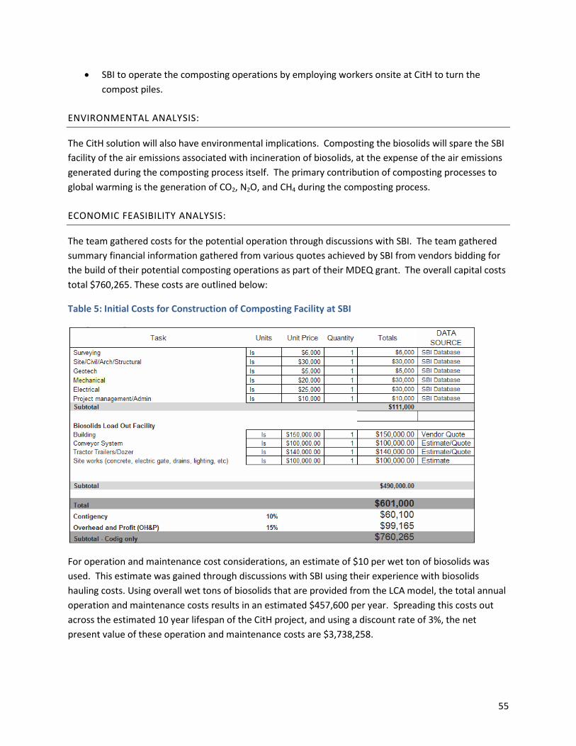
55
• SBI to operate the composting operations by employing workers onsite at CitH to turn the compost piles.
ENVIRONMENTAL ANALYSIS:
The CitH solution will also have environmental implications. Composting the biosolids will spare the SBI facility of the air emissions associated with incineration of biosolids, at the expense of the air emissions generated during the composting process itself. The primary contribution of composting processes to global warming is the generation of CO2, N2O, and CH4 during the composting process.
ECONOMIC FEASIBILITY ANALYSIS:
The team gathered costs for the potential operation through discussions with SBI. The team gathered summary financial information gathered from various quotes achieved by SBI from vendors bidding for the build of their potential composting operations as part of their MDEQ grant. The overall capital costs total $760,265. These costs are outlined below:
Table 5: Initial Costs for Construction of Composting Facility at SBI
For operation and maintenance cost considerations, an estimate of $10 per wet ton of biosolids was used. This estimate was gained through discussions with SBI using their experience with biosolids hauling costs. Using overall wet tons of biosolids that are provided from the LCA model, the total annual operation and maintenance costs results in an estimated $457,600 per year. Spreading this costs out across the estimated 10 year lifespan of the CitH project, and using a discount rate of 3%, the net present value of these operation and maintenance costs are $3,738,258.

56
As the conveyor systems also use electricity, the team estimated that the conveyors would operate at 10 horsepower, or 7.5kW of power, 5 days per week75. This will result in an estimated 46,800 kWh of electricity used per year, which results in about $4680 in electricity costs over the course of one year, using $0.10/kWh as a baseline.
3.5.3. KILN DRYING
Kiln drying is a method by which SBI can upgrade their digested class B biosolids into Class A biosolids. Class A biosolids can in turn be delivered to higher-value markets, such as fertilizer for farming of crops for human consumption, soil amendments for gardens, parks, or other green spaces. This movement into another market may open avenues for SBI to garner financial profits from their digestate solid waste.
Kiln drying involves a few key components: the Class B biosolids on the input, a fuel that can be combusted to generate heat, a system by which that heat is transferred to the biosolids, and a sturdy enclosure in which the biosolids are heated. After a set period of time at high temperatures, the pathogens present within the biosolids are killed, rendering the resulting product safer for more applications. Kiln drying systems typically use natural gas or other fossil-derived fuel to provide the heat needed to achieve the required level of pathogen reduction. However, the kiln drying system can readily replace natural gas with biogas that is generated during SBI’s digestion process. This can result in a symbiotic system that utilizes waste products from one process as a value-added fuel in another process.
ASSUMPTIONS:
• Kiln drying system capable of processing one ton per hour of biosolids • Estimated cost of a kiln drier of this size: $300,000 • Kiln drying system estimated to use about 1 mmBTU of natural gas per hour • Natural gas can be substituted with biogas from the digestion process • Unable to land apply in winter months • For more information on calculations associated with substituting biogas into the kiln dryer, see
Section 3.6.3.
ENVIRONMENTAL ANALYSIS:
Environmental impacts of kiln drying must also be considered when determining how it fares against other biosolids disposal options. The air emissions associated with incineration of the biosolids are
75 Powertran. “Powertran Application of the Conveyor Belt.” 2010. Web. <http://www.inverter-china.com/application-of-conveyor.htm>.

57
spared with relation to the Base Case scenario. However, kiln drying results in emissions via the combustion of natural gas or biogas to supply heat to upgrade to Class A biosolids. The kiln drying system is estimated to handle 1 ton per hour of biosolids at a natural gas usage rate of 1 mmBTU per hour.
ECONOMIC FEASIBILITY ANALYSIS:
Along with the kiln drying system, SBI would also need about 2.2 million gallons of biosolids storage to hold the biosolids during the winter months when biosolids are not demanded. This involves a significant upfront investment. As a low-end cost estimate, the UM team used a baseline of $1.50 per gallon for storage costs76, resulting in an overall upfront capital expenditure of $3.3 million. In total, a kiln drying system would cost about $2.5 million initial investment cost.
Operation and maintenance (O&M) would also be a significant cost contributor for a kiln drying solution. The first category of O&M costs would be the usage of natural gas in the kiln-dryer. Assuming a natural gas inlet rate of 1 mmBTU per hour to support a biosolids inlet rate of 1 ton per hour, using natural gas as a fuel would become necessary if biogas is not utilized. In addition, a staff of about 2 individuals will be needed to operate and maintain the kiln drying system on a daily basis, doing such activities as daily cleaning, diagnostics, and transfer from the kiln dryer to storage if needed, as well as monitoring and maintaining the 2.2 million gallon storage tanks. If these individuals work for 40 hours per week at a rate of $15/hour, then the total labor cost associated with kiln drying would be estimated $62,400/year. Totaling the fuel cost and labor cost together, the estimated yearly cost for operation and maintenance of the kiln drying system would be the price of natural gas plus an additional $62,400 per year.
3.5.4. ENERGY CROPS
Prior to researching the environmental impact and economic feasibility of growing energy crops at CitH in depth we conducted a preliminary literature review to compare growing energy crops as feedstock supplies vs. growing corn for ethanol production. According to a paper that reviewed the benefits of co-digestion using energy crops, feedstock supplementation mitigates fluctuations in feedstock supplies, is more cost effective, can dilute inhibitory compounds, provides nutrient balance, increases biodegradation, and improves methane productivity. Furthermore, energy crops can be stored through the ensiling process (controlled fermentation during silo storage) as a stock during high demand.77 In addition, we believe that growing energy crops for digestion instead of growing energy crops for ethanol would be more in line with SBI’s prime directive to produce biogas. According to another study, Research is being conducted to evaluate which species of plants would grow best in Michigan. As of
76 Ross, Brian. Gennesee County Drain Commission, Personal Communication. January 23rd, 2012.
77 Nges, Ivo Achu, Federico Escobar, Xinmei Fu, and Lovisa Björnsson. "Benefits of Supplementing an Industrial Waste Anaerobic Digester with Energy Crops for Increased Biogas Production." Waste Management (2011). Print.
58
now, Miscanthus x giganteus (corn) and switchgrass are seen as the most promising.78 Given that maize is already widely grown in the state, we determined that it would be the most suitable energy crop to investigate.
ASSUMPTIONS:
• Due to restrictions in land suitable for crop production and area needed for transportation we assumed 100 of the 130 acres at CitH would be used to grow maize.
• Fertilizer would not be needed as biosolids would provide sufficient nutrients • SBI would not incur any costs associated with owning CitH • SBI would use the same trucks they are using to transport biosolids to CitH • Transportation of maize from CitH to the biogas plant would be coupled with transportation of
biosolids to CitH • There is no limit to the amount of time maize could be ensiled before digestion • Centrate composition would be roughly the same as sludge
ENVIRONMENTAL ANALYSIS:
We used peer-reviewed publications to quantify environmental impact associated maize production, transportation, storage, and digestion. When a range of numbers was given, we chose highest number to display what optimal yield would be.
Given published numbers for dry tons of maize per acre and MCF of biomethane per dry ton, we calculated the approximate amount of energy that would be consumed. We treated maize feedstock as food waste input and unless otherwise noted used the same numbers for both.
Due to limited research on energy crop use for anaerobic digestion in the United States, many literature sources we collected from are based on studies conducted in Europe. Therefore, numbers used are an approximation.
ECONOMIC FEASIBILITY ANALYSIS:
As maize is an annual crop, lifetime of the project was set to one year. Capital costs comprised of a corn combine at $140,000. The cost of growing maize uses numbers that were projected for the year 2011 and include pesticides, seed, drying, machine repair, labor, buildings, storage, machinery depreciation,
78 Extension.org. "Miscanthus for Biofuel Production - Extension." Extension.org. Web. 15 Apr. 2012. <http://www.extension.org/pages/26625/miscanthus-for-biofuel-production>.
59
non-land interest, and overhead. 79 Costs associated with growing maize totaled $42,300. Revenue was calculated for the percentage of biomethane or electricity produced from energy crops over total input. Prices were based on the most recent (Spring, 2012) electricity and natural gas prices in the U.S.
3.5.5. PHOSPHORUS RECOVERY: OSTARA PELLETIZER
Phosphorus Recovery can provide a value added product in the biosolids disposal process. The process of thickening and dewatering sludge results in a centrate, which is highly concentrated in nutrients including phosphorus and nitrogen. Typically this centrate is returned to the head of the wastewater treatment plant and treated again before being discharged in the effluent of the wastewater treatment plant. This adds particular load and strain to the wastewater treatment plant, requiring additional energy to manage the biochemical oxygen demand (BOD) to tolerable effluent limits. Extracting phosphorus and nitrogen from the nutrient rich centrate can be an effective method of decreasing plant load, lowering the concentration of phosphorus and nitrogen in the effluent, and producing a valuable product that can be sold as organic fertilizer.
Nutrient recovery is a relatively new technology and is motivated by several economic and environmental factors. Wastewater treatment plants discharging effluent into biologically stressed or sensitive water bodies are sometimes required to lower effluent concentrations of phosphorus and limiting nutrients to levels far below federal regulations. Algal blooms and high BOD levels can have a severe environmental impact and can negatively impact ecological systems and services. The cost of nutrient removal for wastewater treatment plants can be costly, but nutrient recovery technologies can mitigate these costs by creating value added products such as fertilizers. Additionally, phosphorus is a finite and declining resource which if essential to agricultural production. Concerns over global food security are closely tied to the production of phosphorus which some studies forecast a resource constraint in the next 50 to 100 years.80
ASSUMPTIONS:
• Concentration of phosphorus in the centrate and from the sludge thickener averaged 460 mg/l per the elemental analysis conducted by SBI.81
• The nutrient removal efficiency of the Ostara Pelletizer ® is 95%.82
79 UIUC. "Per Acre Cost to Grow Corn and Soybeans." UIUC.edu. Web. <http://fbfm.ace.uiuc.edu/pdf%20files/Farm%20Business%20Results/Cost%20of%20Production%20for%20Grain/c&s_north.pdf>.
80 Dana Cordell, J.-O. D. (2008, May 27). The story of phoshorus: Global food security and food for thought. Linkoping, Sweden.
81 City of Flint Wastewater Treatment Plant. “Calorific Value and Elemental Analysis of the City of Flint WPCD Sludge Cake.” 2011. Print.

60
• Electricity would be used for heating input of the Ostara Pelletizer. • Transportation of the final product would be the responsibility of a third party and therefore
falls outside of the SBI boundary. • Economics were based on the generic reported numbers from Durham Advanced Wastewater
Treatment Facility • The product would contain 28% available phosphorus (P2O5) and is of high enough quality to
offset P2O5 fertilizer production for agricultural inputs (100% P2O5 product ratio) • The price per ton of product was estimated at $800/ton based on the Farmers Coop Grain
Association historical fertilizer prices of similar NPK composition (10-34-0).83
ENVIRONMENTAL ANALYSIS:
We investigated the opportunity for SBI operation in Flint, Michigan to invest in nutrient recovery technology using Ostara ® Nutrient Recovery Technologies as a resource for implementing such a system. Our model incorporated the economic and environmental impact of installing and operating a Pearl Reactor™ system for the purpose of nutrient recovery and resale of fertilizer product. We used the best available data to calculate the value of the resulting fertilizer product. To estimate the capital, operational, and maintenance costs of the operation we referenced case studies from installed systems at the Durham Wastewater Treatment near Portland Oregon. Primary data from Ostara® was used to calculate the energy requirements, fertilizer composition and nutrient removal efficiency.
ECONOMIC FEASIBILITY ANALYSIS:
The cost of installing the Ostara Pelletizer was approximated to the publically available project cost posted by the Durham, Oregon Advanced Wastewater Treatment Plant operated by CleanWater Services. The facility cost $2.5 million and had an expected payback time of five years. Specific details of the project were not available for review; however the plant size of the Durham facility is similar in size to the Flint WWTP but with a much higher average daily flow. $2.5 million was used as a very conservative estimate to evaluate the economic cost. The economic benefit was calculated using best available information on prices of fertilizer from the Farmers Coop Grain Association.
82 Crystal Green. “How it’s Made”. Web. 2012. <http://www.crystalgreen.com/content/how-its-made>.
83 Farmers Coop Grain Assoc. “Historical Fertilizer Prices. 2012. Web. <http://www.wellingtoncoop.com/index.php?page=ferthist.php>.

61
3.6. MODELING BIOGAS USAGE
3.6.1. BIOGAS USE IN THE CURRENT OPERATIONS
In the current operations, biogas was either used in the boiler to heat the digesters or flared. We assumed that SBI would choose to use biogas instead of natural gas to heat the digester. Biogas available was first allocated for use in the boiler to serve the primary purpose of heating the digesters. The rest of the biogas was flared. See section 3.4.3 for details on boiler operation and emissions from the boiler for biogas or natural gas.
Emissions from the flaring of biogas were estimated by multiplying the amount of biogas flared each year by emissions factors for criteria pollutants and greenhouse gases derived from literature and GREET1_2011 model of natural gas flaring in oil field.84 85 All of the CO2 content in biogas was assumed to pass through the boiler and into the air as CO2. We also assumed that the total hydrogen sulfide (H2S) content of biogas was released as SO2. Stoichiometric calculations were used to convert the volume of CO2 and H2S per 1 MCF of biogas to pounds of CO2 and SO2 per 1 MCF of biogas. The resulting CO2 emissions factor was added to the CO2 emissions factor from the GREET1_2011 model. (See Appendix 2: Emission Factors for a table of emission factors for biogas flaring.)
3.6.2. BIOGAS USE IN THE FULLY OPERATIONAL CASE
Modeling for the electricity generator was based on the specifications for the continuous 1600 eKW model G3520 C low energy fuel Caterpillar generator. The generator runs at full capacity at 14.744 MCF of biogas per hour. A linear regression of % load of the generator and biogas input revealed that the minimum biogas input was 2 MCF/hr. When active, the generator ran continuously for 97% of the year and, as a CHP unit, produced waste heat for use in heating the digesters.86 The heat delivered to the water jacket to heat the digesters was scaled based on the percent loading of the generator. The electrical output of the generator was based on the 660 MBtu/MCF heating value for biogas and a 41% efficiency of the generator. Emissions for the combustion of biogas in the generator were based on the specifications for the generator, except for CO2, CH4 and SO2. The emission factor for CH4 was found in peer-reviewed literature. 87 Stoichiometric calculations were used to convert the volume of CO2 and H2S per 1 MCF of biogas to pounds of CO2 and SO2 per 1 MCF of biogas.
84 Electrigaz Technologies Inc. "Feasibility Study – Biogas Upgrading and Grid Injection in the Fraser Valley, British Columbia." Electrigaz. 2007. Web. <www.lifesciencesbc.ca/files/PDF/feasibility_study_biogas.pdf>.
85 Argonne National Laboratory. “GREET1_2011 Model.” 2011. Web. < http://greet.es.anl.gov/>.
86 Antle, Chad. Personal phone communication. 2011.
87 Nielsen, M., and J. B. Illerup. "Danish Emission Inventories for Stationary Combustion Plants, Inventories until Year 2001." National Environmental Research Institute192nd ser. (2003). Print.
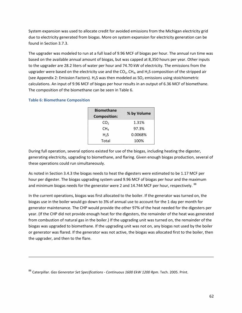
62
System expansion was used to allocate credit for avoided emissions from the Michigan electricity grid due to electricity generated from biogas. More on system expansion for electricity generation can be found in Section 3.7.3.
The upgrader was modeled to run at a full load of 9.96 MCF of biogas per hour. The annual run time was based on the available annual amount of biogas, but was capped at 8,350 hours per year. Other inputs to the upgrader are 28.2 liters of water per hour and 74.70 kW of electricity. The emissions from the upgrader were based on the electricity use and the CO2, CH4, and H2S composition of the stripped air (see Appendix 2: Emission Factors). H2S was then modeled as SO2 emissions using stoichiometric calculations. An input of 9.96 MCF of biogas per hour results in an output of 6.36 MCF of biomethane. The composition of the biomethane can be seen in Table 6.
Table 6: Biomethane Composition
Biomethane Composition:
% by Volume
CO2 1.31% CH4 97.3% H2S 0.0068%
Total 100%
During full operation, several options existed for use of the biogas, including heating the digester, generating electricity, upgrading to biomethane, and flaring. Given enough biogas production, several of these operations could run simultaneously.
As noted in Section 3.4.3 the biogas needs to heat the digesters were estimated to be 1.17 MCF per hour per digester. The biogas upgrading system used 9.96 MCF of biogas per hour and the maximum and minimum biogas needs for the generator were 2 and 14.744 MCF per hour, respectively. 88
In the current operations, biogas was first allocated to the boiler. If the generator was turned on, the biogas use in the boiler would go down to 3% of annual use to account for the 1 day per month for generator maintenance. The CHP would provide the other 97% of the heat needed for the digesters per year. (If the CHP did not provide enough heat for the digesters, the remainder of the heat was generated from combustion of natural gas in the boiler.) If the upgrading unit was turned on, the remainder of the biogas was upgraded to biomethane. If the upgrading unit was not on, any biogas not used by the boiler or generator was flared. If the generator was not active, the biogas was allocated first to the boiler, then the upgrader, and then to the flare.
88 Caterpillar. Gas Generator Set Specifications - Continuous 1600 EkW 1200 Rpm. Tech. 2005. Print.

63
3.6.3. BIOGAS USE FOR ALTERNATIVE AND SUPPLEMENTAL OPERATIONS
Based on the 1mmBtu/hour needs of the kiln dryer (See Section 3.5.3) and a 660 MBtu heating value for biogas, the kiln dryer used 1.515 MCF biogas/hr. Biogas allocation with kiln-drying followed the same pattern as in the Fully Operational case, except that the kiln-dryer would use the biogas remaining after use by the generator and upgrader (if turned on). If any biogas remained after use by the kiln-dryer, it was flared.
3.7. SYSTEM EXPANSION ALLOCATION METHODOLOGY
System expansion can be used in LCA application when modeling indirect environmental burdens associated with the functional unit. However, the use of system expansion to identify indirect and marginal effects can be restricted to the acceptability of the expansion and feasibility of results. For the purposes of this study, the recovery of valuable nutrients from biosolids, which is traditionally seen as a waste product, is seen to have significant environmental benefits. We therefore applied a system expansion to the kiln drying and phosphorus recovery system to provide a quantitative comparison to the creation of synthetic nitrogen and mined phosphorus. For kiln drying the predominant recovery nutrient is nitrogen being returned to the environment when it is land applied. The Ostara® Pelletizer produces a product with a high concentration of phosphorus. A description of how each system expansion is provided in the following section.
3.7.1. KILN DRYING SYSTEM EXPANSION
Because kiln drying generates a readily marketable product and can be applied anywhere Class A biosolids are accepted. Heat dried pellets can contain up to 6% nitrogen and 5% phosphorus. Because these nutrients are being returned to the ecological cycle as a fertilizer this can create an offset for synthetically created fertilizer. For the purposes of this analysis, the amount of nitrogen content in the resulting dried biosolids was used to offset the production of synthetic nitrogen.
Cradle to gate life cycle emissions were compiled for 100% nitrogen to product production ratio using agricultural inputs from the Argonne National Laboratory GREET 1 model. The resulting quantity of available nitrogen in the dried biosolids was then multiplied by the emission factors of nitrogen production to determine the total emissions offset from the kiln drying nutrient recovery process.

64
Table 7: Elemental Analysis of Dewatered Biosolids
Element Moisture Free wt %
Carbon 36.19%
Hydrogen 5.12% Nitrogen 3.74% Oxygen 23.51% Sulfur 1.52%
𝐴𝑛𝑛𝑢𝑎𝑙 𝑠𝑙𝑢𝑑𝑔𝑒 𝑝𝑟𝑜𝑐𝑒𝑠𝑠𝑒𝑑 (𝐷𝑟𝑦 𝑇𝑜𝑛𝑠) ∗ 3.74% 𝑏𝑦 𝑤𝑒𝑖𝑔ℎ𝑡 𝑛𝑖𝑡𝑟𝑜𝑔𝑒𝑛 (𝑆𝐵𝐼 𝐸𝑙𝑒𝑚𝑒𝑛𝑡𝑎𝑙 𝐴𝑛𝑎𝑙𝑦𝑠𝑖𝑠)= 𝑇𝑜𝑡𝑎𝑙 𝑛𝑖𝑡𝑟𝑜𝑔𝑒𝑛 𝑟𝑒𝑐𝑜𝑣𝑒𝑟𝑒𝑑𝑝𝑒𝑟 𝑦𝑒𝑎𝑟
𝑇𝑜𝑡𝑎𝑙 𝑛𝑖𝑡𝑟𝑜𝑔𝑒𝑛 𝑟𝑒𝑐𝑜𝑣𝑒𝑟𝑒𝑑 ∗ 𝑒𝑚𝑖𝑠𝑠𝑖𝑜𝑛 𝑓𝑎𝑐𝑡𝑜𝑟𝑠 𝑓𝑜𝑟 𝑠𝑦𝑛𝑡ℎ𝑒𝑡𝑖𝑐 𝑛𝑖𝑡𝑟𝑜𝑔𝑒𝑛 𝑝𝑟𝑜𝑑𝑢𝑐𝑡𝑖𝑜𝑛(𝐺𝑅𝐸𝐸𝑇 1)= 𝐴𝑛𝑛𝑢𝑎𝑙 𝑒𝑚𝑖𝑠𝑠𝑖𝑜𝑛 𝑜𝑓𝑓𝑠𝑒𝑡 (𝑡𝑜𝑛𝑠)
3.7.2. PHOSPHORUS RECOVERY SYSTEM EXPANSION
Similar to the kiln drying, a system expansion was used to calculate the offset of environmental burdens associated with phosphorus production. The fertilizer product produced by the Ostara Pearl® reactor contains 28% available phosphorus (P2O5). This is a significant nutrient recovery from the centrate and separated water from sludge thickening that would otherwise be returned to the head of the wastewater treatment plant. Using the total available phosphorus available in the final fertilizer product and the emission factors associated with 100% phosphorus (P2O5) production, the offset was subtracted from the overall emissions associated with operating the Ostara system.
Table 8: Crystal Green® Technical Data
Crystal Green® Technical Data Total Nitrogen (N) 5%
Available Phosphate (P2O5) 28%
Soluble Potash (K2O) 0% Magnesium (Mg) 10%
𝐴𝑛𝑛𝑢𝑎𝑙 𝐶𝑦𝑟𝑠𝑡𝑎𝑙 𝐺𝑟𝑒𝑒𝑛 𝑝𝑟𝑜𝑑𝑢𝑐𝑡𝑖𝑜𝑛(𝑡𝑜𝑛𝑠) ∗ 28% (𝑎𝑣𝑎𝑖𝑙𝑎𝑏𝑙𝑒 𝑝ℎ𝑜𝑠𝑝ℎ𝑎𝑡𝑒)= 𝐴𝑛𝑛𝑢𝑎𝑙 𝑟𝑒𝑐𝑜𝑣𝑒𝑟𝑒𝑑 𝑝ℎ𝑜𝑠𝑝ℎ𝑎𝑡𝑒(𝑡𝑜𝑛𝑠)
𝐴𝑛𝑛𝑢𝑎𝑙 𝑎𝑣𝑎𝑖𝑙𝑎𝑏𝑙𝑒 𝑝ℎ𝑜𝑠𝑝ℎ𝑎𝑡𝑒 (𝑡𝑜𝑛𝑠) ∗ 100% 𝑃2𝑂5𝑝𝑟𝑜𝑑𝑢𝑐𝑡 𝑝𝑟𝑜𝑑𝑢𝑐𝑡𝑖𝑜𝑛 𝑒𝑚𝑖𝑠𝑠𝑖𝑜𝑛 𝑓𝑎𝑐𝑡𝑜𝑟= 𝑇𝑜𝑡𝑎𝑙 𝑎𝑛𝑛𝑢𝑎𝑙 𝑒𝑚𝑖𝑠𝑠𝑖𝑜𝑛 𝑜𝑓𝑓𝑠𝑒𝑡

65
3.7.3. ELECTRICITY GENERATION SYSTEM EXPANSION
A system expansion was used to calculate the offset of environmental burdens associated with combustion of fossil fuels for the Michigan electricity grid due to the electricity generation from biogas.
To calculate the avoided emissions, the amount of electricity generated was calculated (as described in Section 3.6.2) and multiplied by the emission factors for the Michigan grid (see Appendix 2: Emission Factors). These emissions were then subtracted from the electricity emissions from other processes in the system.
3.8. ENVIRONMENTAL IMPACT ASSESSMENT MODELING
The environmental impacts of emissions generated at each life cycle stage were assessed using the following midpoint characterization factors: global warming potential, acidification potential, and smog formation potential. These midpoints represent the most relevant, feasibly quantifiable and adequately representative metrics applicable to our study. All will be quantified per 1 MCF of biogas (our functional unit) and for the life cycle stage they are associated with. If an emitted gas is contributes to more than one impact metric, it will be counted toward both midpoints. For example, methane emissions will be counted as a contributor to both global warming potential and smog formation potential.
To determine all equivalencies, the annual emissions for each gas were multiplied by a characterization factor that represents their relative contribution to each impact metric. Local and site-specific conditions were not taken into consideration.
Midpoints were calculated using characterization factors from the EPA’s Tool for the Reduction and Assessment of Chemical and Other Environmental Impacts (TRACI).89 One of the most prominent reasons for choosing TRACI against other impact assessment tools is that its methodologies for calculating midpoints for acidification and smog formation are specifically tailored for the United States. (Due to influence on atmospheric conditions, global warming is based on universal impact.) Furthermore, TRACI has highly defensible methodologies and was designed with the most up to date LCA methods.90
89 U.S. EPA. “TRACI 2.0.xls.” spreadsheet from U.S. EPA. 2012.
90 U.S. EPA. “Tool for the Reduction and Assessment of Chemical and Other Environmental Impacts (TRACI).” 2012. Web. <http://www.epa.gov/nrmrl/std/traci/traci.html>.

66
Global warming potentials are based on the IPCC 2007 report using a 100-year time horizon.91 Characterization factors for GWP were based on the IPCC and not TRACI since their methodology was more comprehensive.
Table 9: Impact Assessment Midpoints
Impact Assessment Description Unit Reference Global Warming Potential (GWP)
A measure of greenhouse gas emissions, such as CO2 and methane. These emissions are causing an increase in the absorption of radiation emitted by the earth, magnifying the natural greenhouse effect.
kg CO2 equivalent IPCC92
Acidification Potential (AP)
A measure of emissions that cause acidifying effects to the environment. The acidification potential is assigned by relating the existing S-, N-, and halogen atoms to the molecular weight.
mol H+ equivalent EPA TRACI93
Smog Potential (PCOP)
A measure of emissions of precursors that contribute to low level smog, produced by the reaction of nitrogen oxides and VOC’s under the influence of UV light.
kg O3 equivalent EPA TRACI94
For a table of characterization factors see Appendix 4: Impact Characterization Factors.
3.9. CONVERSION TO FUNCTIONAL UNIT
LCA results for the Fully Operational and Alternative and Supplementary scenarios were put in terms of the functional unit, 1 MCF of biogas produced. For the results in terms of functional unit, the emissions and energy use from Base Case are considered to be avoided emissions and are subtracted from each of the Fully Operational and Alternative and Supplementary Scenarios. Since biogas is not produced in the Base Case, a functional unit comparison was used to evaluate the Base Case operations model with that of current and future operations of the SBI plant. We used dry tons per day input as a reference flow to evaluate energy use and emissions across all scenarios. The following methodology was used to
91 IPCC. “Direct Global Warming Potentials.” IPCC. 2007. Web. <http://www.ipcc.ch/publications_and_data/ar4/wg1/en/ch2s2-10-2.html>.
92 IPCC. “Direct Global Warming Potentials.” IPCC. 2007. Web. <http://www.ipcc.ch/publications_and_data/ar4/wg1/en/ch2s2-10-2.html>. 93 U.S. EPA. “TRACI 2.0.xls.” spreadsheet from U.S. EPA. 2012.
94 U.S. EPA. “TRACI 2.0.xls.” spreadsheet from U.S. EPA. 2012.

67
calculate the emissions associated with biogas production for the Current and Future operation scenarios.
𝐵𝑎𝑠𝑒 𝐶𝑎𝑠𝑒 𝑅𝑒𝑓𝑒𝑟𝑒𝑛𝑐𝑒 𝐹𝑙𝑜𝑤 = 9𝐷𝑇𝑑𝑎𝑦
∗ 365𝑑𝑎𝑦𝑠𝑦𝑒𝑎𝑟
= 3,285𝐷𝑇𝑦𝑒𝑎𝑟
(𝑠𝑙𝑢𝑑𝑔𝑒 𝑖𝑛𝑝𝑢𝑡)
𝐸𝑚𝑖𝑠𝑠𝑖𝑜𝑛𝑠 (𝐵𝐶)𝑦𝑒𝑎𝑟
3,285 𝐷𝑇𝑦𝑒𝑎𝑟
=𝐸𝑚𝑖𝑠𝑠𝑖𝑜𝑛𝑠 (𝐵𝐶)
𝐷𝑇
DT= Dry Tons
Emissions (BC) = Total associated emissions resulting from electricity use and incineration
Current Operations Reference Flow was calculated using the same procedure.
𝐶𝑢𝑟𝑟𝑒𝑛𝑡 𝐶𝑎𝑠𝑒 𝑅𝑒𝑓𝑒𝑟𝑒𝑛𝑐𝑒 𝐹𝑙𝑜𝑤 = 9.0 𝐷𝑇𝑑𝑎𝑦
∗ 365 𝑑𝑎𝑦𝑠𝑦𝑒𝑎𝑟
= 3,285 𝐷𝑇𝑦𝑒𝑎𝑟
(𝑠𝑙𝑢𝑑𝑔𝑒 𝑖𝑛𝑝𝑢𝑡)
𝐸𝑚𝑖𝑠𝑠𝑖𝑜𝑛𝑠 (𝐶𝐶)𝑦𝑒𝑎𝑟
3,285 𝐷𝑇𝑦𝑒𝑎𝑟
=𝐸𝑚𝑖𝑠𝑠𝑖𝑜𝑛𝑠 (𝐶𝐶)
𝐷𝑇
Emissions (CC) = Total emissions associated resulting from electricity, incineration, and biogas combustion in boiler and flare
To find the net emissions associated with biogas production the Base Case Emissions was subtracted from the Current operations:
𝐸𝑚𝑖𝑠𝑠𝑖𝑜𝑛𝑠 (𝐶𝐶)𝐷𝑇
− 𝐸𝑚𝑖𝑠𝑠𝑖𝑜𝑛𝑠 (𝐵𝐶)
𝐷𝑇= 𝑁𝑒𝑡 𝐸𝑚𝑖𝑠𝑠𝑖𝑜𝑛𝑠 (𝐶𝑢𝑟𝑟𝑒𝑛𝑡)
𝐷𝑇
Using net emissions associated with current biogas production we calculated the emissions associated with each MCF of biogas produced in the Current operations.
𝐵𝑖𝑜𝑔𝑎𝑠 𝑃𝑟𝑜𝑑𝑢𝑐𝑒𝑑 (𝐶𝐶)𝑀𝐶𝐹/𝑦𝑒𝑎𝑟𝐷𝑇/𝑦𝑒𝑎𝑟
=𝑀𝐶𝐹 𝐵𝑖𝑜𝑔𝑎𝑠(𝐶𝐶)
𝐷𝑇
𝑁𝑒𝑡 𝐸𝑚𝑖𝑠𝑠𝑖𝑜𝑛𝑠 𝐶𝑢𝑟𝑟𝑒𝑛𝑡𝐷𝑇
∗𝐷𝑇
𝑀𝐶𝐹 𝐵𝑖𝑜𝑔𝑎𝑠 (𝐶𝐶)=𝑁𝑒𝑡 𝐸𝑚𝑖𝑠𝑠𝑖𝑜𝑛𝑠 𝐶𝑢𝑟𝑟𝑒𝑛𝑡
𝑀𝐶𝐹 𝐵𝑖𝑜𝑔𝑎𝑠
This method can be used to evaluate the Fully Operational and Alternative and Supplementary scenarios as well.

68
3.10. BIOGENIC CARBON
The U.S. Environmental Protection Agency’s Deferral for Carbon Dioxide Emissions From Bioenergy and Other Biogenic Sources Under the Prevention of Significant Deterioration and Title V Program defines biogenic CO2 as the “CO2 from a stationary source directly resulting from the combustion or decomposition of biologically-based materials other than fossil fuels and mineral sources of carbon.” Some of the examples included in this definition are:
• “CO2 generated from the biological decomposition of waste in landfills, wastewater treatment or manure management processes
• CO2 from the combustion of biogas collected from biological decomposition of waste in landfills, wastewater treatment or manure management processes”95
At the time of this publication, the global warming impact potential of biogenic CO2 was still under review by the EPA’s Scientific Advisory Board, and there is still much debate in the scientific community as to whether biogenic CO2 should be counted as net zero. The primary argument for counting biogenic carbon as net zero involves looking at the life cycle of biological systems. The growth of biomass sequesters CO2 and therefore, during the life of the biomass, the incineration or decomposition of the biomass will never exceed the CO2 sequestered by the biomass. The primary argument against accounting biogenic carbon as net zero involves the rate of release into the atmosphere. Biogenic carbon that is combusted is released instantly into the atmosphere whereas natural biodegradation can take many years.
The boundary of this project does not include the carbon sequestration resulting from the human, food, and organic waste. However the resulting carbon in the biosolids and biogas products are considered to be biogenic. In this report the results for CO2 emissions are categorized into two categories, biogenic and anthropogenic. We decided this was the best representation of biogenic carbon because of the discrepancies in opinion and consensus among the scientific community on the contribution of biogenic carbon to global warming potential.
Contributions from biogenic carbon are reported separately in the Life Cycle Inventory phase but do contribute to the overall Global Warming Potential in the Life Cycle Impact Assessment phase of the LCA. The reason for reporting the results in this matter allowed the user and audience to determine their own conclusions on the role of biogenic carbon on Global Warming Potential.
95 U.S. EPA. “Carbon Dioxide Accounting for Emissions from Biogenic Sources.” U.S. EPA Science Advisory Board. 2012. Web. <http://yosemite.epa.gov/sab/sabproduct.nsf/0/2F9B572C712AC52E8525783100704886? OpenDocument>.

69
3.11. SENSITIVITY ANALYSES
In order to determine the robustness of our results, we have performed several key sensitivity analyses.
METHANE PRODUCTION POTENTIAL
We chose 1 MCF of biogas as the functional unit for the product system. Thus, the results of the study are likely to be highly dependent on the amount of biogas produced by the system. We assume that the methane production potential of one ton of volatile solids in sludge is 9,600 cubic feet, and the methane production potential of one ton of volatile solids in food waste is 14,000 cubic feet. We examined the change in our model results after varying methane production potential of sludge in the current operations scenario and food waste in the Fully Operational with Generator scenario (one at a time) by +/- 10% in increments of 2.5%.
PERCENT VOLATILE SOLIDS OF TOTAL SOLIDS
Percent of volatile solids of total solids is an important metric that determines the mass of volatile solids in a ton of food waste or sludge, which, along with the methane production potential, determines the amount of methane produced per dry ton of sludge. We observed the change in our model results after varying percent volatile solids of total solids of sludge in the current operations scenario and food waste in the Fully Operational with Generator scenario (one at a time) by +/- 10% in increments of 2.5%.
VOLATILE SOLIDS DESTROYED IN DIGESTION
Percent of volatile solids destroyed in digestion determines the reduction in total solids in the system. This impacts the loads on equipment in stages after digestion, including amount of solids to be incinerated, kiln-dried, or transported to Chevy–in-the-Hole. We examined the change in our model results after varying percent volatile solids destroyed for sludge in the current operations scenario and food waste in the Fully Operational with Generator scenario (one at a time) by +/- 10% in increments of 2.5%.
FUNCTIONAL UNIT
The handling and disposal of solid waste could be viewed as another function of this product system. In this context, the functional unit to consider would be 1 dry ton of waste of input to the system. We investigated the change in our model results when using 1 dry ton of waste input to the system instead of one thousand standard cubic feet (MCF) of biogas produced.

70
4. RESULTS
The Environmental Impact Assessment Model was used to evaluate the three main scenarios: Base Case, Current Operations, and Fully Operational. Five sub-scenarios within the Fully Operational case are assessed:
1) Allocation of biogas to the generator 2) Allocation of biogas to the upgrader 3) Optimal allocation of biogas to the generator or boiler while kiln drying 4) Optimal allocation of biogas to the generator or boiler while growing and using energy crops in
the digester 5) Optimal allocation of biogas to the generator or boiler recovering phosphorus.
4.1. LIFE CYCLE INVENTORY ANALYSIS
4.1.1. BASE CASE
In order to determine the inventory results for the Base Case, the model was set as seen in Table 10 with 9 dry tons of primary sludge input (see
Table 11), which were subsequently dewatered and incinerated. This scenario resulted in 8.55 dry tons of sludge sent to the incinerator each day (see Table 12).
Table 10: Base Case Dashboard
Table 11: Base Case Input Values

71
Table 12: Base Case Output Values
The greenhouse gas emissions for Base Case can be seen in Figure 7. Approximately 11,800 tons of CO2 per year were released, of which about 4,100 tons were biogenic emissions from the combustion of the sludge. Nearly 360 tons of N2O were released while only 300 lb of CH4 were emitted. Large amounts of NOx and CO were also released due to sludge combustion and lack of control devices on the stack for these substances (see Figure 8).
Figure 7: Base Case Greenhouse Gas Emissions

72
Figure 8: Base Case Criteria Pollutant Emissions
4.1.2. CURRENT OPERATIONS
In order to determine the inventory results for current operations, the model was set as seen in Table 13 with sludge going to the digester and biogas used in the boiler. Inputs to the system were 8 dry tons of primary sludge and 1 dry ton of sludge skimmings per day (see
Table 14). After thickening the 1 ton of skimmings, a total of 8.95 dry tons of sludge per day were sent to the digester.
Table 13: Current Operations Dashboard
Table 14: Current Operations Input Values

73
Table 15: Current Operations Output Values
Under current operations, 3.58 MCF of biogas were produced per hour. The boiler used 1.17 MCF/hr and the rest (2.41 MCF/hr) was flared. The model shows implementation of anaerobic digestion reduced the amount of biosolids sent to the incinerator by 2.85 dry tons/day and centrate output increased by 30.42 tons/day compared to Base Case (Table 12 and Table 15).
The greenhouse gas emissions for current operations can be seen in Figure 9. Approximately 10,200 tons of CO2 per year were released, of which 4,700 tons were biogenic emissions from combustion of biogas and sludge. Thus, fossil fuel CO2 emissions dropped by about 2,200 tons/yr compared to Base Case. In addition, annual N2O emissions were reduced by 120 tons through implementation of anaerobic digestion. However, CH4 emissions rose from 300 lbs in Base Case to more than 900 tons in current operations. Criteria pollutants levels were similar to those found in Base Case (see Figure 10), except NOx, SOx and CO emissions fell slightly.
Figure 9: Current Operations Greenhouse Gas Emissions

74
Figure 10: Current Operations Criteria Pollutant Emission
4.1.3. FULLY OPERATIONAL WITH GENERATOR AND BROWNFIELD APPLICATION
The first sub-scenario for Fully Operational includes the use of both digesters, imported food waste, and all of the biogas sent to the generator for electricity production (Table 16). The daily stream input was 8 dry tons of primary sludge, 1 dry ton of sludge skimmings, and 14.5 dry tons of food waste (see Table 17). After thickening the 1 ton of skimmings, a total of 23.45 dry tons/day of sludge and food waste were sent to the digester.
Table 16: Dashboard for Fully Operational with Generator

75
Table 17: Input Values for Fully Operational with Generator
Table 18: Output Values for Fully Operational with Generator
The model showed that in the Fully Operational case with biogas allocation to the generator, almost twice as much digested cake was produced compared to current operations (see Table 15 and Table 18). This cake was transported from the Flint Wastewater Treatment Plant to Chevy in the Hole for brownfield application. More importantly, biogas production nearly quadrupled compared to current operations, generating more than 9,000 MWh per year.
The greenhouse gas emissions for Fully Operational with Generator can be seen in Figure 11. Approximately 4,000 tons of biogenic CO2 per year were released and almost 6,000 tons of CO2 emissions per year were avoided for a net avoidance of 2,000 tons CO2 per year. This represents a 12,000 ton decrease in CO2 emissions compared to current operations. N2O emissions were also 215 tons lower than in current operations. However, methane emissions rose by 365 tons per year. Criteria pollutant levels dropped dramatically for NOx and SOx while VOC and NH3 emissions increased significantly compared to both Base Case and current operations (see Figure 12).
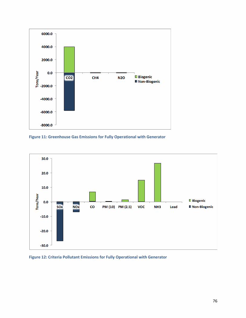
76
Figure 11: Greenhouse Gas Emissions for Fully Operational with Generator
Figure 12: Criteria Pollutant Emissions for Fully Operational with Generator

77
4.1.4. FULLY OPERATIONAL WITH UPGRADER AND BROWNFIELD APPLICATION
The second sub-scenario for Fully Operational includes the use of both digesters, imported food waste, and upgrading of the biogas to biomethane (Table 19). 8 dry tons of primary sludge, 1 dry ton of sludge skimmings, and 14.5 dry tons of food waste was the daily system input (see Table 20). After thickening the 1 ton of skimmings, a total of 23.45 dry tons/day of sludge and food waste were sent to the digester.
Table 19: Dashboard for Fully Operational with Upgrader
Table 20: Input Table for Fully Operational with Upgrader
Table 21: Output Table for Fully Operational with Upgrader
Under the Fully Operational with upgrader scenario, 13.83 MCF of biogas were produced per hour, most of which was processed by the upgrading unit, creating more than 53,000 MCF of biomethane in one year. The remaining 1.53 MCF biogas/hr was flared. Output of biosolids and centrate was the same as for the Fully Operational with Generator scenario (Table 21).
The greenhouse gas emissions for Fully Operational with Upgrader can be seen in Figure 13. Approximately 7,900 tons of biogenic and 2,250 tons of fossil fuel-derived CO2 were released each year. At 25 tons/yr, SOx emissions were higher for this scenario than any other case (see Figure 14). Similar to Fully Operational with Generator, VOC and NH3 emissions were much higher than in Base Case and current operations.

78
Figure 13: Greenhouse Gas Emissions for Fully Operational with Upgrader
Figure 14: Criteria Pollutant Emissions for Fully Operational with Upgrader

79
4.1.5. FULLY OPERATIONAL WITH GENERATOR AND KILN DRYING
The third sub-scenario for Fully Operational includes the use of both digesters, imported food waste, kiln drying the digestate for sale as compost, and the remainder of the biogas sent to the generator for electricity production (Table 22). 8 dry tons of primary sludge, 1 dry ton of sludge skimmings, and 14.5 dry tons of food waste was the daily system input (see Table 23). After thickening the 1 ton of skimmings, a total of 23.45 dry tons/day of sludge and food waste were sent to the digester.
Table 22: Dashboard for Fully Operational with Generator and Kiln Drying
Table 23: Input Table for Fully Operational with Generator and Kiln Drying
Table 24: Output Table for Fully Operational with Generator and Kiln Drying
Under the Fully Operational with Generator and Kiln Drying scenario, 13.83 MCF of biogas/hr were created, with 1.52 MCF biogas/hr allocated to the kiln dryer and the rest to the generator (see Table 24). Even with reduced biogas loading as compared to running only the generator, more than 8,000 MWh of electricity were produced annually. Output of biosolids and centrate was the same as for the Fully Operational with Generator only. However, the resulting biosolids were a 95% dry Class A compost material.
The greenhouse gas emissions for Fully Operational with Generator and Kiln Drying can be seen in Figure 15. More than 5,000 tons of fossil and biogenic CO2 were avoided each year. Biogenic CH4 and N2O were also reduced in this scenario compared to current operations. Criteria pollutant levels, except for VOC and NH3, were similar to those found for Fully Operational with Generator only (see Figure 16). The VOC and NH3 emissions for kiln drying are the lowest for any of the Fully Operational scenarios.

80
Figure 15: Greenhouse Gas Emissions for Fully Operational with Generator and Kiln Drying
Figure 16: Criteria Pollutant Emissions for Fully Operational with Generator and Kiln Drying

81
4.1.6. FULLY OPERATIONAL WITH GENERATOR AND USE OF ENERGY CROPS
The fourth sub-scenario for Fully Operational includes the use of both digesters, imported food waste and energy crops for digester feedstock, and all of the biogas sent to the generator for electricity production (Table 25). 8 dry tons of primary sludge, 1 dry ton of sludge skimmings, 10.35 dry tons of food waste, and 2.2 dry tons of energy crops were the daily system input (see Table 26). After thickening the 1 ton of skimmings and 3.5 tons of primary sludge, a total of 21.33 dry tons/day of sludge, food waste and energy crops were sent to the digester.
Table 25: Dashboard for Fully Operational with Generator and Energy Crops
Table 26: Input Table for Fully Operational with Generator and Energy Crops
Table 27: Output Table for Fully Operational with Generator and Energy Crops
Under the Fully Operational with Generator and Energy Crops scenario, 10.83 MCF of biogas/hr were created, with all of the biogas allocated to the generator (see Table 27). At this rate of generator loading 7,137 MWh of electricity were produced annually, almost 2 GWh less than in the Fully Operational with Generator only case. Output of biosolids and centrate were the same as the Fully Operational with Generator only.
The greenhouse gas emissions for Fully Operational with Generator and Phosphorus Recovery can be seen in Figure 17. Approximately 4,000 tons/yr of biogenic CO2 were released and almost 4,000 tons/yr of CO2 emissions were avoided, which results in a net of zero CO2 emissions. Criteria pollutant levels were similar to those found in the Fully Operational with Generator only case, except with a smaller quantity of avoided SOx and NOx (see Figure 18).

82
Figure 17: Greenhouse Gas Emissions for Fully Operational with Generator and Energy Crops
Figure 18: Criteria Pollutant Emissions for Fully Operational with Generator and Energy Crops

83
4.1.7. FULLY OPERATIONAL WITH GENERATOR AND PHOSPHORUS RECOVERY
The fifth sub-scenario for Fully Operational includes the use of both digesters, imported food waste, phosphorus recovery from the centrate, and all of the biogas sent to the generator for electricity production (Table 28). The daily system input was 8 dry tons of primary sludge, 1 dry ton of sludge skimmings, and 14.5 dry tons of food waste (see Table 29). After thickening the 1 ton of skimmings, a total of 23.45 dry tons/day of sludge and food waste were sent to the digester.
Table 28: Dashboard for Fully Operational with Generator and Phosphorus Recovery
Table 29: Input Table for Fully Operational with Generator and Phosphorus Recovery
Table 30: Output Table for Fully Operational with Generator and Phosphorus Recovery
Under the Fully Operational with Generator and Phosphorus Recovery scenario, 13.83 MCF of biogas/hr were created (see Table 30). The biogas was allocated entirely to the generator, producing more than 9,000 MWh of electricity annually. Output of biosolids and centrate was the same as for the Fully Operational with Generator only. However, the centrate is passed through a phosphorus recovery system where much of the water is evaporated in the process of drying out the nutrients for recovery.
The greenhouse gas emissions for Fully Operational with Generator and Phosphorus Recovery can be seen in Figure 19. Approximately 4,000 tons/yr of biogenic CO2 were released and almost 6,000 tons/yr of CO2 emissions were avoided for a net avoidance of 2,000 tons CO2 per year. Criteria pollutant levels were similar to those found in the Fully Operational with Generator only case (see Figure 20).

84
Figure 19: Greenhouse Gas Emissions for Fully Operational with Generator and Phosphorus Recovery
Figure 20: Criteria Pollutant Emissions for Fully Operational with Generator and Phosphorus Recovery

85
4.1.8. NON-RENEWABLE ENERGY USE
4.1.8.1. NATURAL GAS CONSUMPTION
There is a large variance in natural gas consumption across the different scenarios, reflecting the amount of biogas produced and its allocation (Figure 21). Base Case consumed more natural gas than any other case (~130,000 MCF/year). Current operations showed a drastic reduction in consumption with a difference of approximately 40,000 MCF per year. Even greater reductions, more than 1 x 10⁵ MCF per year, are seen in the Fully Operational cases compared to the Base Case.
Natural gas consumed per MCF produced showed improvements all cases compared to the Base Case, with fully operational scenarios showing greater reductions than the current operations (Figure 22). Current operations showed an improvement of approximately 1.7 MCF. Fully operational scenarios showed improvements of ~3.5 MCF. The greatest reduction in natural gas consumption was in phosphorus recovery with an improvement of ~3.7 MCF.
Figure 21: Annual Natural Gas Consumption by Case

86
Figure 22: Natural Gas Consumption per MCF of Biogas Produced by Case
4.1.8.2. ELECTRICITY CONSUMPTION
Electricity was consumed annually in the Base Case, current operations, and Fully Operational case at approximately 1 MWh, 500 MWh, and 2,000 MWh per year respectively (Figure 23). The remaining cases displayed negative values from electricity credits. Fully operational with electricity generation had the lowest value for consumption with roughly -7,300 MWh/yr. Kiln Drying, energy crops, and phosphorus recovery had credits leading to impacts ranging from roughly -5,700 MWh/yr for energy crops and phosphorus recovery and -6,700 MWh for kiln drying.
Electricity per MCF was consumed in the current operations and Fully Operational case with upgrading at 12.7 and 17.2 kWh respectively (Figure 24). The remaining cases displayed negative values from electricity credits. Fully operational with electricity generation had the lowest value at -63 kWh/MCF though did not show as proportionally large a difference from the other cases as in annual electricity consumption. Kiln drying, energy crops, and phosphorus recovery had values of -54 kWh/MCF, -58 kWh/MCF, -63 kWh/MCF, respectively.

87
Figure 23: Annual Electricity Consumption by Case
Figure 24: Electricity Consumption per MCF Produced by Case

88
4.1.8.3. DIESEL CONSUMPTION
All fully operational cases consumed at least 20,000 times more gallons of diesel per year than the base and current operations (Figure 25). The base and current operations consumed ~200 x103 gallons per year. Energy crops and phosphorus recovery consumed about 6 million gallons per year. Fully operational with generator, fully operational with upgrader, and fully operational with kiln drying consumed ~8.5 million gallons per year.
All fully operational cases consumed 60-70 times more gallons of diesel per MCF produced than the current operations, which had a value of nearly zero (Figure 26). Energy crops and phosphorus recovery consumed about 64 gallons per MCF. Fully operational with generator, fully operational with upgrader, and fully operational with kiln drying consumed about 70 gallons per MCF.
Figure 25: Annual Diesel Consumption by Case

89
Figure 26: Diesel Consumption per MCF Produced by Case
4.2. LIFE CYCLE IMPACT ASSESSMENT
4.2.1. GLOBAL WARMING POTENTIAL
Annual global warming potential showed a wide range of emissions across the different cases (Figure 27). Biogenic emissions accounted for a vast majority of emissions. Base Case emitted the most at nearly 120,000 tons of CO2 eq per year. Current operations emitted more than three times more CO2 eq than all Fully Operational cases, and emitted nearly as much as Base Case with 104,000 tons CO2 eq. Fully operational with electricity generation, kiln drying, energy crops and phosphorus recovery displayed negative non-biogenic emissions due to credits from electricity generation.
In accounting for GWP per MCF, all cases showed substantial improvements from the Base Case. These ranged from nearly 1000 lb CO2 eq/MCF for the current operations to roughly 5,700 lb CO2 eq/MCF for energy crops and phosphorus recovery (Figure 28). A majority of improvements are attributed to biogenic sources.
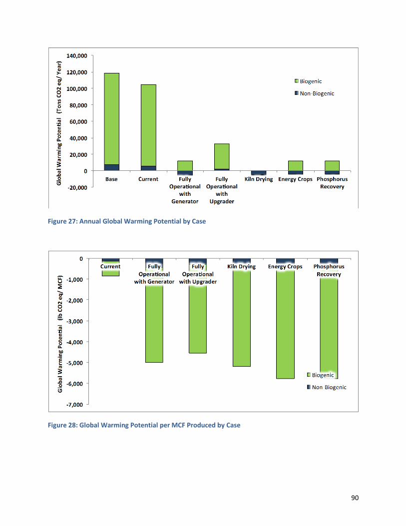
90
Figure 27: Annual Global Warming Potential by Case
Figure 28: Global Warming Potential per MCF Produced by Case

91
4.2.1. ACIDIFICATION POTENTIAL
The cases displayed a variety of acidification potential values (Figure 29). Fully operational with upgrading is responsible for the greatest amount emissions at roughly 1,700 mol H+ eq/year. Kiln drying accounted for the most avoided acidification potential. Fully operational with electricity generation, energy crops, and phosphorus recovery also had negative acidification potential values, though they were only from non-biogenic sources. The three cases emitted positive biogenic emissions. Base Case and current operations had biogenic and non-biogenic acidification potentials.
All cases showed avoided acidification potentials compared to the Base Case (Figure 30). These improvements from the Base Case ranged from roughly -12 mol H+ eq/MCF for Fully Operational with Upgrader to -38 mol H+ eq/MCF for phosphorus recovery.
Figure 29: Annual Acidification Potential by Case
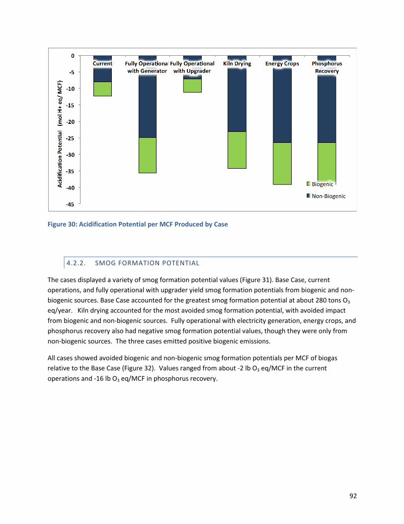
92
Figure 30: Acidification Potential per MCF Produced by Case
4.2.2. SMOG FORMATION POTENTIAL
The cases displayed a variety of smog formation potential values (Figure 31). Base Case, current operations, and fully operational with upgrader yield smog formation potentials from biogenic and non-biogenic sources. Base Case accounted for the greatest smog formation potential at about 280 tons O3 eq/year. Kiln drying accounted for the most avoided smog formation potential, with avoided impact from biogenic and non-biogenic sources. Fully operational with electricity generation, energy crops, and phosphorus recovery also had negative smog formation potential values, though they were only from non-biogenic sources. The three cases emitted positive biogenic emissions.
All cases showed avoided biogenic and non-biogenic smog formation potentials per MCF of biogas relative to the Base Case (Figure 32). Values ranged from about -2 lb O3 eq/MCF in the current operations and -16 lb O3 eq/MCF in phosphorus recovery.
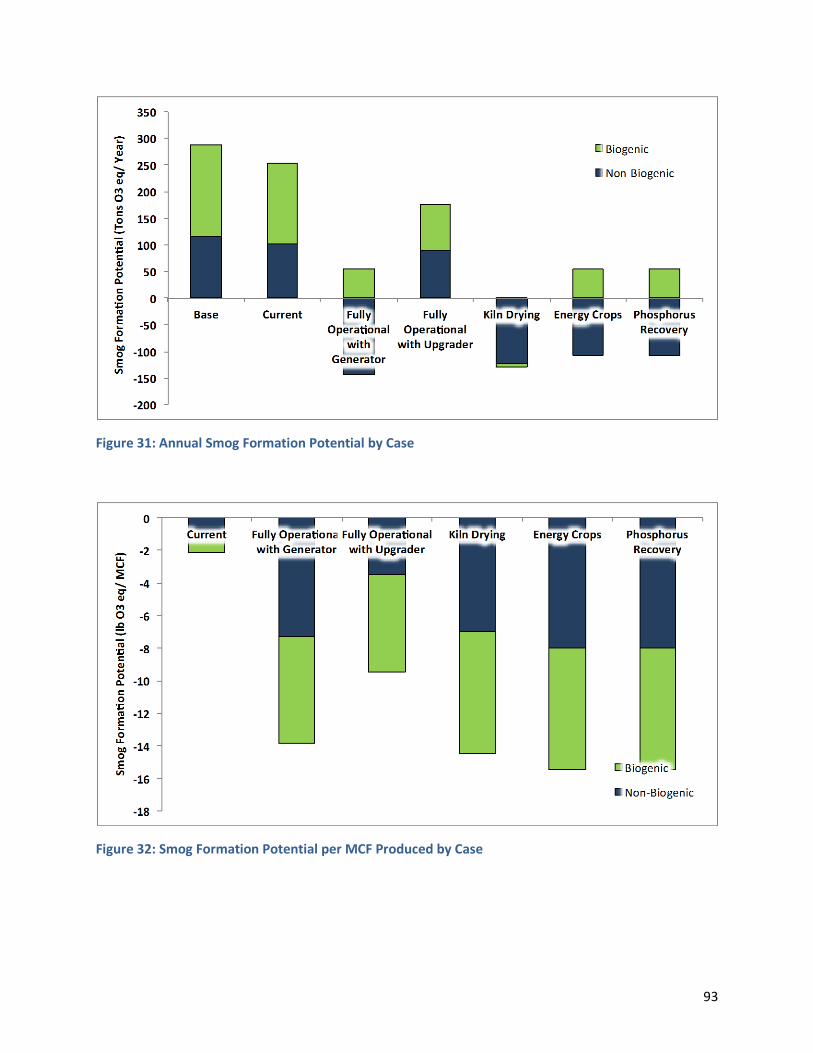
93
Figure 31: Annual Smog Formation Potential by Case
Figure 32: Smog Formation Potential per MCF Produced by Case

94
4.3. SENSITIVITY ANALYSES
4.3.1. METHANE PRODUCTION POTENTIAL, %VS OF TS, AND %VS DESTRUCTION
Model outputs of biogas production (MCF/hr) and the three impact categories were tested for their sensitivity to changes in methane production potential (MPP), % volatile solids of total solids (%VS of TS), and % VS destruction. In current operations, the biogas output was not very sensitive to changes in sludge MPP and sludge %VS of TS (see Figure 33). Biogas output was not at all sensitive to changes in %VS destroyed as it is not dependent upon that value.
Figure 33. Sensitivity Analysis of Biogas Production in Current Operations
Figure 34. Sensitivity Analysis of Global Warming Potential in Current Operations

95
In current operations, GWP was fairly sensitive to changes in sludge MPP and sludge %VS destroyed (see Figure 34). Avoided impact level increased considerably with increasing % VS destroyed, suggesting that the disposal of biosolids in the incinerator contributes significantly to GWP. Avoided impact level decreased with increasing sludge MPP. This result occurs because higher MPP leads to more biogas production. As GWP was calculated per MCF of biogas, so the avoided impact from Base Case is divided across a greater quantity of biogas, causing the avoided impact to decrease. (See Appendix 5: Sensitivity Analyses for the sensitivity analysis results for acidification potential and smog formation potential.)
In Fully Operational with Generator, the biogas output was not very sensitive to changes in sludge MPP and sludge %VS of TS (see Figure 35). Biogas output was not at all sensitive to changes in %VS destroyed as it is not dependent upon that value.
Figure 35. Sensitivity Analysis of Biogas Production in Fully Operational with Generator
Figure 36. Sensitivity Analysis of Global Warming Potential in Fully Operational with Generator
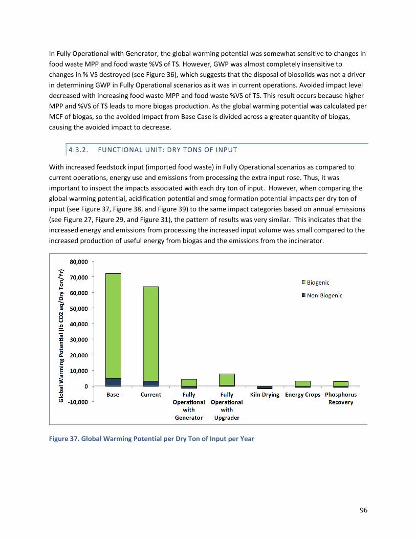
96
In Fully Operational with Generator, the global warming potential was somewhat sensitive to changes in food waste MPP and food waste %VS of TS. However, GWP was almost completely insensitive to changes in % VS destroyed (see Figure 36), which suggests that the disposal of biosolids was not a driver in determining GWP in Fully Operational scenarios as it was in current operations. Avoided impact level decreased with increasing food waste MPP and food waste %VS of TS. This result occurs because higher MPP and %VS of TS leads to more biogas production. As the global warming potential was calculated per MCF of biogas, so the avoided impact from Base Case is divided across a greater quantity of biogas, causing the avoided impact to decrease.
4.3.2. FUNCTIONAL UNIT: DRY TONS OF INPUT
With increased feedstock input (imported food waste) in Fully Operational scenarios as compared to current operations, energy use and emissions from processing the extra input rose. Thus, it was important to inspect the impacts associated with each dry ton of input. However, when comparing the global warming potential, acidification potential and smog formation potential impacts per dry ton of input (see Figure 37, Figure 38, and Figure 39) to the same impact categories based on annual emissions (see Figure 27, Figure 29, and Figure 31), the pattern of results was very similar. This indicates that the increased energy and emissions from processing the increased input volume was small compared to the increased production of useful energy from biogas and the emissions from the incinerator.
Figure 37. Global Warming Potential per Dry Ton of Input per Year
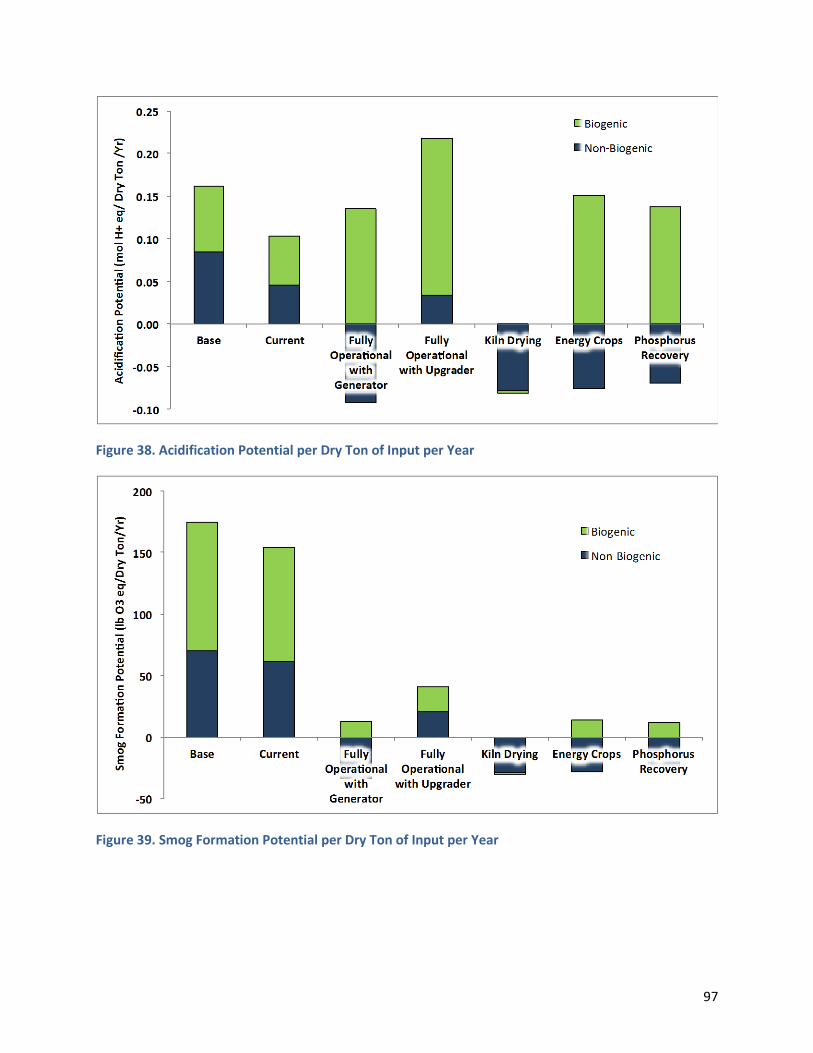
97
Figure 38. Acidification Potential per Dry Ton of Input per Year
Figure 39. Smog Formation Potential per Dry Ton of Input per Year

98
5. ADDITIONAL BIOSOLID MANAGEMENT SCENARIOS
In addition to modeling various biosolids management contingencies, we investigated several alternatives qualitatively based on the results from the multi-criteria decision analysis. The purpose of this exercise was to investigate possible opportunities for SBI based on the economic, environmental and overall feasibility. The below selected alternatives were chosen based on a range of similar projects across the country, unique ideas brought forth by the study team based on previous knowledge and ideas from the SBI leadership team to identify possible opportunities within the operational framework of SBI in Flint, Michigan.
5.1. PASTUERIZATION OF CENTRATE TO A CLASS A
The centrate or reject stream from dewatered biosolids can contribute to higher ammonia and phosphorus loads at a wastewater treatment plant, weakening secondary treatment performance. Finding opportunities to minimize this return to the head works of the wastewater treatment can offer significant operational efficiency benefits and reduce high-level ammonia and phosphorus effluent concentrations. There is also the potential for the creation of value added products, which can be utilized as a Class A liquid fertilizer.
While the dewatering flow or centrate contributes to less than one percent of the flow to most WWTPs it has the potential of contributing 15-30% of the nitrogen load.96 There are several methods of using a separate treatment system to manage the ammonia/nitrogen and phosphorus levels in the centrate stream. Physical and chemical solutions include hot air and stream stripping, struvite precipitation, or chlorination. There are also several biological treatments as well including SHARON®, InNitri ® and several others (Technologies). In addition to these opportunities for dealing with the increased ammonia and nitrogen loading, we propose a pasteurization using existing heat from the combined heat and power (CHP) unit.
The waste heat rejected from the CHP can offer a valuable heat source to pasteurize the centrate to a level adequate to meet Class A standards. The centrate could then be land applied to areas in need of nutrient recovery. Significant further studies would need to be investigated on the basis of the pathogen levels within the centrate to determine the appropriate pasteurization process. Initial analysis shows that the 2280 MBTU/hour is more than sufficient to provide ample thermal energy for heating the digestion process and pasteurization of the centrate.
Challenges to pasteurization of the centrate include increased environmental monitoring systems to ensure minimum federal regulations are met; constructing, operating and maintaining a pasteurization system; and managing the transportation, allocation and disposal of the centrate while observing the seasonal limitations for disposal (regulations do not allow biosolids to be land applied during the winter). With an average processing volume of 65,000 gallons of centrate per day, the process of
96 Constantine, T. (2006). North American Experience with Centrate Treatment. North York: CH2M Hill.

99
pasteurization, storage and land application requires a significant allocation of resources and planning. Our initial analysis of the local, regional and federal regulations revealed that though feasible, this is not a viable solution to produce a value added product from biogas production. The current demand for fertilizer and the political and social conditions of the area surrounding Flint, Michigan make marketing this product very difficult.
In conclusion, until a viable market becomes available for the land application of Class A biosolids near the Flint WWTP, pasteurization of the centrate is not a viable option. The required infrastructure, monitoring and distribution means are relatively costly investments for a limited confidence level on market feasibility. Additionally, this might become a viable option if the Flint WWTP begins to struggle to maintain proper effluent levels. Further research into the net present value and internal rate of return is suggested if nutrient removal becomes an issue due to the advent of anaerobic digestion.
5.2. GREENHOUSE GAS EMISSIONS REDUCTION FROM TREE PLANTATION IN CITH
Even with the use of biogas as a fuel for the Flint WWTP, the SBI facility will continue to have onsite GHG emissions in the form of CO2 from the combustion of the biogas. Though the methane combusted is biogenic, there is still a scientific debate if this contributes to global warming by being expelled into the atmosphere. There is therefore an opportunity for SBI to utilize all its waste products in a beneficial way to contribute to a truly zero-waste principle of operation. In such a scenario, the plant contributes to a notion of industrial symbiosis, where waste products from one process can be used as an input to another process.
With this guiding principle, SBI could pursue a number of options for the use of its waste CO2. One such option is the routing of waste CO2 to greenhouses in which trees are grown. These trees can then be planted at CitH. This aligns with the City of Flint’s goal of planting trees at CitH to enhance its appeal as a green space, and also serves as a useful way to uptake excess CO2. Additionally, waste heat from CHP operations can be utilized to heat the greenhouses to optimal temperatures, displacing the usage of natural gas in heaters that would otherwise run for the same purpose. This option can result in potentially significant carbon savings, especially if the planting of trees at CitH is already planned.
There are several challenges to implementing this option, however. First, there are numerous logistical hurdles to overcome to make such a symbiotic system work. The piping and distribution system of the CO2 from the SBI facility to the greenhouse must be constructed at a likely high cost. Further, piping waste heat from CHP processes would also serve an extremely challenging tasks over long distances, which may require the greenhouse facilities to be nearby, if not attached to, the SBI facility. This may result in location issues and difficulties in running both a wastewater treatment operation and an agricultural operation simultaneously. Finally, it is not certain the degree by which the trees will uptake excess CO2, as there are several varieties that could be chosen for the CitH site. It is likely that the greenhouse option will only likely account for a small percent of overall carbon emitted, leaving a significant percentage that still needs to be captured to achieve a truly zero-waste effort.

100
Overall, the option for GHG capture for trees may only by beneficial if the City of Flint already plans on a large-scale tree planting operation at CitH. It will likely result in marginal carbon savings with a high capital investment. It may serve as a useful enterprise if SBI can secure long-term clients to use the greenhouse facilities after tree planting at CitH is completed. But the strengths with greenhouses would be largely political, as the costs of running the operating the greenhouse would overcome the revenues in the short-term.
5.3. CLASS B – LAND APPLICATION FARM/FOREST
As a contingency to applying the biosolids to CitH, SBI can also apply its biosolids to farm/forestland in the Flint Area. The land application could occur with the Class B biosolids just as they are after the digestion process.
The benefits of land application on farm or forestland are that these environments can readily realize benefits from the nutrients of biosolids, using it as a sort of soil fertilizer. Due to the pathogens in the biosolids that can be harmful to human health, the biosolids must lay upon the land for a set period of time before that land can be safe for regular human use. For that reason, areas such as forest are good candidates for disposal, because they are isolated from populated areas, allowing biosolids to rid of their pathogens in a safe environment. The nutrients in the biosolids also help to increase crop yields in farms and to increase overall habitat liveliness in forests by increasing soil fertility and plant production.
The drawbacks of land application in farm or forestland are that each plot of land comes with its own distinct needs that will need to be fully understood. Some areas may be conservation areas and may be akin to tighter regulations. Other areas may have unclear boundaries on where humans tread the land and where they don’t, making selected sites for waste disposal more difficult. Also, it is unclear exactly how much forest and farmland would be available and would demand Class B biosolids. Lastly, there may be a planning challenge in ensuring that biosolids can be reliably disposed of long-term. That is, SBI or the City of Flint would need to employ a strategy for applying biosolids to new land areas after others have reached their capacity. Lastly, there continues to be a public stigma associated with farmland that is fertilized with biosolids, even if it the crop is not directly consumed by humans. For that reason, it may be challenging to promote widespread adoption at farmland throughout the Flint area.
Overall, application of Class B biosolids in farm or forestland is a reasonable alternative for disposing of biosolids at CitH. It requires hardly any new equipment or capital purchases, and only requires the identification of disposal sites before it can proceed. However, due to uncertainties and political sensitivities of Class B land application of biosolids, we recommend that the municipalities in the Flint Area and SBI work together to determine the best sites for disposal if moving forward with a land application strategy.

101
5.4. CLASS A – OUTDOOR COMPOSTING
As of April 2012, SBI has suspended plans to upgrade their biosolids to Class A through composting. However, there is a growing market for Class A compost in Michigan and should SBI compost in the future, it would be well suited to respond to demand.
Due to the vast tracts of fenced-off land at CitH, a high volume of available bulking agent in the form of yard waste from the City of Flint, adaptability to changes in biosolids characteristics, low dependency on mechanical equipment, and low capital costs, SBI would likely compost through windrows. This entails piling the biosolids and bulking agent mixture into long rows and mechanically turning the biosolids in order to provide oxygen to the aerobic bacteria for digestion. EPA 503 regulations to produce class A require biosolids temperatures to each 55°C for at least 15 days with 5 turns. Other composting methods (aerated static pile and in-vessel) would require higher capital cost and maintenance but they would have a faster turnaround time and in some cases produce less odor.97
With the absence of detectable pathogens, Class A compost has a wider variety of applications than Class B biosolids. Currently, Class A and B compost is distributed to farmers and gardeners in Michigan at no cost, which makes it an unprofitable method to dispose of biosolids. However, with a predicted increase in the cost of fertilizer, SBI and WWTPs in Michigan may be able to start charging. Fertilizer prices have been increasing over the past decade and the U.S. has had difficulty meeting sharp increases in demand.98 Recently, a record high was reached in 2009 at $185 per ton. Moreover, using 2011 reports from USDA and the University of Illinois prices are predicted to reach $162 per acre in 2012, exceeding those of 2010 and 2011.99 Other cities demonstrate that composting biosolids to Class A can be profitable. Though working with a much larger volume, the Milwaukee Metropolitan Sewerage District has made a thriving business (Milorganite) from manufacturing slow-release organic nitrogen fertilizer from biosolids.100 At times demand exceeds supply.101 Furthermore, there is growing encouragement from the state government. Michigan’s Department of Environmental Quality (MDEQ) encourages beneficial use of biosolids and is working to reverse the negative public perception of fertilizer and other products made from biosolids.
97 U.S. EPA. “Biosolids Technology Fact Sheet.” U.S. EPA. 1999. Web. <http://water.epa.gov/scitech/wastetech/upload/2002_10_15_mtb_combioman.pdf>.
98 USDA. “Factors Contributing to the Recent Increase in Fertilizer Prices.” USDA. 2009. Web. <http://www.ers.usda.gov/Publications/AR33/AR33.pdf>.
99 Dairy Business. “Looking Ahead – 2012 Fertilizer Futures Prices Higher” Dairy Business. 2011. Web. <http://dairybusiness.com/features/2011-07-14/looking-ahead--2012-fertilizer-futures-prices-higher>.
100 Milorganite. “About.” Milorganite. 2012. Web. <http://www.milorganite.com/About>.
101 Dr. Zamani, Bahram. Head of Michigan Biosolids Management Program for Genessee County and Middle Michigan, Michigan Department of Environmental Protection. Personal phone communication. 2011.

102
5.5. CLASS B – SUPERFUND SITES
The EPA’s Superfund program assesses, tracks the progress of, and implements the proper procedures to clean up sites contaminated with substances hazardous to human health and the environment. There are currently over 80 Superfund sites in Michigan on the National Priorities List (NPL), which identifies the most hazardous sites that are candidates for long-term remediation. Pending investigation by the EPA, these or others in the region may be remediated in part with biosolids. Due to the hazardous nature of the site and regulations prohibiting public access prior to clean up, the biosolids would be Class B.
Superfund has used biosolids to accelerate re-vegetation at their sites by providing benefits such as nutrients for plants, a buffer for acidity, and conditions that help decrease extractable metals in soil.102 Applying biosolids from the SBI plant would help the company promote their green image. Furthermore, it may be one of the most economically feasible alternatives since the parties responsible for contamination at the site are responsible for covering the costs for remediation.
Procedures to investigate and develop a plan to clean up the sites are very time intensive, which would make it a less attractive option. The EPA must conduct a remedial investigation/feasibility study to characterize site conditions, classify the waste, assess health and environmental risks, and evaluate treatment technology implementation feasibility and cost.103 The probability finding sites suitable for biosolids use is unknown until these procedures are carried out.
5.6. URBAN AGRICULTURE
As an alternative to applying biosolids at CitH for its future reclamation as a green space, the City of Flint and SBI could instead work together to implement an urban agriculture program on CitH. Urban agriculture is the growing of crops on smaller plots of land in urban environments. It is a growing trend in many cities as a method by which to reclaim unused land. In the case of SBI, the biosolids output from the WWTP operation would be used as a fertilizer on agriculture land set aside at CitH. The agriculture operation can vary depending on whether SBI chooses to upgrade its biosolids to Class A or Class B. If Class A is delivered as fertilizer, the urban agriculture plots could support human-based agriculture such as vegetables, fruit, herbs, or other food items that can be sold directly to food vendors. If Class B is delivered as fertilizer, the urban agriculture plots would be more focused on
102 Brown, Sally, Charles Henry, Rufus Chaney, Harry Compton, and Pam De Volder. "Using Municipal Biosolids in Combination with Other Residuals to Restore Metal-Contaminated Mining Areas." Plant and Soil 429 (2003): 203-15. USDA. 2003. Web. <http://ddr.nal.usda.gov/bitstream/10113/15429/1/IND23343062.pdf>.
103 U.S. EPA. “Remedial Investigation/Feasibility Study” U.S. EPA. 9 Aug. 2011. Web. <http://www.epa.gov/superfund/cleanup/rifs.htm>.

103
producing crops that can be used as animal feed purposes, such as corn or oats that can be delivered to other farms for their livestock.
Urban agriculture operations are often viewed as beneficial for struggling communities looking to rebuild, by promoting the creation of jobs, offering local fresh food as an alternative to processed store-bought foods, and generally increasing livelihood and productivity of youth in their respective neighborhoods. These benefits would definitely be observed in an urban agriculture program in Flint. As the City of Flint is politically positioned to create jobs and attract citizens back to the city, urban agriculture presents an opportunity to attract useful work in the short-term on the unused land at CitH. In terms of technical feasibility, urban agriculture represents a reasonable alternative, as the logistics of applying to farmland at CitH should be similar to applying to empty land aiming to be a future green space.
There are several challenges and uncertainties associated with implementing urban agriculture. There is significant uncertainty in the market for local crops in CitH grown using biosolids, and whether urban agriculture will serve to be financially viable and profitable. It is also unclear who will manage the urban agriculture plots, whether they are private owners, SBI, or the City of Flint. Also, it is quite certain that the rate at which biosolids are being produced at the WWTP will be much higher than the demand for biosolids at the urban agriculture plots, especially during the winter months. So, SBI would need a backup contingency strategy in its portfolio to ensure all of its biosolids can be sustainably managed at any time of year. This would result in logistical challenges for the organization.
Overall, an urban agriculture program would be most beneficial if strategically agreed to by all parties involved. The main motivator for urban agriculture is political in nature, as its benefits revolve around the increased sense welfare amongst the citizens. Developing this strategy is important for moving forward with the program. In particular, it would be essential to establish the details of who would own the land and develop a long-term, financially supported goal for the CitH.

104
6. DISCUSSION
This section provides a conclusion to the study on the optimum allocation of biosolids and biogas. The results of the alternative and supplemental cases are also examined along with recommendations for future investigation and an overview of key takeaways from the study.
6.1. OPTIMAL ALLOCATION OF BIOSOLIDS
Overall, the five future scenarios displayed a reduction in impact relative to the current operations, which was less impactful than the Base Case. The reduction in impact in the current operations relative to the Base Case is attributed to the reduction of input to the incinerator. Thus, there is a substantial reduction in emissions associated with fossil fuels and natural gas needed to run the incinerator. However, the anaerobic digestion process leads to a more than 600 ton increase in CH4 emissions, most of which is flared off. Despite the increase in CH4 emissions, incinerating digested sludge reduces GWP from both biogenic and fossil fuel sources.
There is a vast improvement in GWP from eliminating incineration all together. This energy intensive process and allocating the digestate and biogas to value-added processes and products reduces GWP by roughly 2-3 tons of CO2 eq per MCF of biogas and at least ~85,000 tons of CO2 eq per year (Figure 27 and Figure 28). Incineration is responsible for nearly all N2O emissions, which have 298 times the GWP of CO2. Nitrous oxide is the primary contributor to GWP in this system and a majority of its can be feasibly avoided. The considerable amount of avoidable impact in the future scenarios, which do not involve incineration, underlines the importance of finding alternate uses for biosolids.
6.2. OPTIMAL ALLOCATION OF BIOGAS
In the Fully Operational scenarios, allocation of biogas to electricity generation is more environmentally beneficial than upgrading to biomethane. There is avoided impact from both fossil fuel and biogenic sources. By generating electricity, credits may be given for avoiding fossil fuel combustion to produce electricity for the grid, which in Michigan is very carbon-intensive. Avoided impact is most apparent in acidification potential and smog formation potential impacts with large reductions in SOx and NOx, and CH4 and NOx, respectively (Figure 30 and Figure 32).
Credits were neither given for the production of biomethane nor the creation of compost from kiln drying. Since the biomethane could be allocated to a variety of sources it is sold, the proper credits were unable to be calculated. If in the future, given more information about where the biomethane would be combusted, the study may be modified to include credits for offsetting the combustion of natural gas. Additionally while the model accounted for emissions associated with combusting biogas for kiln drying, emissions associated with land application were not included. The compost would most likely consist of CO2 emissions and a minimal amount of N2O and CH4, as the compost would digest

105
aerobically rather than anaerobically. Future studies may include assumptions regarding the amount and type of digestion occurring during kiln drying and application and storage of compost.
6.3. ALTERNATE AND SUPPLEMENTARY CASES
6.3.1. KILN DRYING
While kiln drying is an environmentally beneficial means of allocating biosolids, the necessary equipment requires high capital costs. Out of the three alternate scenarios, kiln drying requires the least amount of annual electricity consumption (Figure 23) and out of all scenarios has the least amount of annual GWP (Figure 27). Moreover, the Class A biosolids product could be used in a greater variety of ways and would impose less of a risk to human health and the environment. SBI’s existing knowledge of the composition of sludge and food waste inputs would be useful in quantifying the amount of nutrients present in the compost. This would aid in determining the organic compost’s retail value and how inputs to AD may be improved if their priorities switched to biosolids rather than biogas production.
Despite environmental benefits, cost may be of concern. A $3.3 million storage unit is required to hold about three months worth of compost produced during winter months since land application to farms in the area would not be possible at that time of year. The kiln dryer would cost an additional $300,000, not including maintenance and repair. If SBI were to expand operations to larger cities, economies of scale may make this option possible. The business model has been proven in other cities such as Milwaukee, which has made a thriving business out of producing organic compost known as Milorganite, which is derived from kiln-dried sludge. Otherwise, kiln drying is not an economically attractive option.
6.3.2. PHOSPHORUS RECOVERY
Phosphorus recovery creates a value added product from centrate, which would otherwise be considered a waste product that would have to be reprocessed at the WWTP. Crediting the production of P2O5 allows this case to have the lowest impact in across all three midpoints, tying with energy crops (Figure 28, 30, 32).
Despite environmental advantages, phosphorus recovery is not economically viable on the scale of the plant in Flint. The equipment needed to recover the phosphorus is $2.5 million, which is quite high compared to the estimated $127,000 in annual revenue. However, with a significantly larger volume of centrate and/or higher concentration of phosphorus, this may be an option.
6.3.3. ENERGY CROPS
Though maize production at CitH for AD input is shows little environmental input relative to the other cases, its low percentage of volatile solids does not produce much biogas per unit of input. Energy crops in the case of CitH are carbon neutral and do not diminish the area of land that could be used for food

106
production, thus addressing commonly cited disadvantages. Energy crops also tie with phosphorus recovery in having the lowest impact across all three midpoints (Figures 28, 30, 32).
Energy crops are not cost effective. There are high capital and operation costs for project estimated at approximately $200,000 for its first year. Furthermore, it produces much less biogas per unit of ton of wet input compared to food waste leading to further reductions in potential profit.
There are factors that should be considered in future studies. Biogas production from energy crops may increase with crop rotation such as maize and soy. Also, according to literature, late ripening maize varieties, digesting whole maize, and maximum silage time increases methane yield.104 Data addressing these factors specifically for Michigan would give more accurate results. Also, emissions associated with maize during the ensiling, which were not accounted for in this study, may be significant.
6.4. CONCLUSION
LOCATION AND MARKET CONDITIONS
There are a variety of factors at play that necessitate deviation from operations in Sweden. This is mainly due to an array of market-dependent and location-specific variables.
This report recommends that biogas should be allocated to generate electricity rather than upgraded to biomethane. This option not only reduces emissions, but also is suited to market conditions in the United States. In Sweden electricity is much cheaper and is produced from hydropower and nuclear power, which are much less carbon intensive compared to the grid mix in Michigan. The higher cost of electricity in the U.S. makes it more financially attractive to generate electricity.
While SBI has been successful in working with municipal governments to create a biogas-driven public transportation fleet in Linköping, it would be much more difficult to do so in Flint. Firstly, diesel fuel in Sweden is roughly twice as expensive as gasoline in the U.S. Second, while the City of Flint government may find it environmentally beneficial to implement a green public transportation fleet, the city has neither the concentrated infrastructure nor a sufficient population to make this viable.
A number of biosolids application options are dependent on available financial capital. While SBI’s partnership with the City of Flint has aided in producing revenue, the city’s financial crisis limits the projects SBI can engage in. Currently, an economic emergency manager is auditing and restructuring
104 Amon, Thomas, Vitaliy Kryvoruchko, Barbara Amon, Werner Zollitsch, Erich Potsch. "Biogas Production from Maize and Clover Grass Estimated With the Methane Energy Value System." Web. <http://www.boku.ac.at/fileadmin/_/H93/H931/AmonPublikationen/biogas_production_maize_and_clover.pdf>.

107
Flint’s operations and investments. Though many of the potential projects would provide long-term return of investment, their payback period is longer than desired. Investments in projects with high capital are not feasible at this time. As described in Sections 5, there are a number of projects that can reduce negative environmental impact; however, since they are not economically viable they cannot implemented. In sum, “you have to be in the black to be green.”
FLEXIBILITY IN UTILIZING ANAEROBIC DIGESTION PRODUCTS
The products and byproducts of anaerobic digestion can be used for a diverse array of applications. The environmental impact associated with each of these processes may not be readily apparent for life cycle stages upstream and downstream of what occurs at the plant. Therefore, the life cycle assessment model created specifically for SBI would be useful in determining which course of action to take to minimize negative environmental impact. Moreover, the model is adaptable. With some modification it can fit alternate scenarios that were not included in this study and other biogas plants.

108
7. WORKS CITED
City of Flint Wastewater Treatment Plant. "Annual Report to Michigan Department of Environmental Quality on City of Flint Wastewater Treatment Plant Air Emissions." (2011). Print.
City of Flint Wastewater Treatment Plant. “Calorific Value and Elemental Analysis of the City of Flint WPCD Sludge Cake.” (2011). Print.
Comunities and Local Government. “Multi-criteria analysis: a manual.” Communities and Local Government Publications. 28 Jan. 2009. Web 17 Mar. 2012. <http:// eprints.lse.ac.uk/12761/1/Multi-criteria_Analysis.pdf>.
Amon, Thomas, Vitaliy Kryvoruchko, Barbara Amon, Werner Zollitsch, Erich Potsch. "Biogas Production from Maize and Clover Grass Estimated With the Methane Energy Value System." Web. <http://www.boku.ac.at/fileadmin/_/H93/H931/AmonPublikationen/biogas_production_maize_and_clover.pdf>.
Antle, Chad. Director of Operations. SBI. Personal e-mail and phone communications, Microsoft Excel documents. 2011-2012.
Argonne National Laboratory. “GREET1_2011 Model.” 2011. Web. < http://greet.es.anl.gov/>.
Brown, Sally, Charles Henry, Rufus Chaney, Harry Compton, and Pam De Volder. "Using Municipal Biosolids in Combination with Other Residuals to Restore Metal-Contaminated Mining Areas." Plant and Soil 429 (2003): 203-15. USDA. 2003. Web. <http://ddr.nal.usda.gov/bitstream/10113/15429/1/IND23343062.pdf>.
Brynas, Anna. Lab Manager and Process Engineer. SBI. Peronal e-mail and phone communications. 2011-2012.
Caterpillar. Gas Generator Set Specifications - Continuous 1600 EkW 1200 Rpm. Tech. 2005. Print.
City of Flint Wastewater Treatment Plant. “Annual Report to Michigan Department of Environmental Quality on City of Flint Wastewater Treatment Plant Air Emissions.” (2011). Print.
Constantine, T. “North American Experience with Centrate Treatment” North York: CH2M Hill. 2006.Web. < http://www.environmental-expert.com/Files/5306/articles/13105/423.pdf>.
Dairy Business. “Looking Ahead – 2012 Fertilizer Futures Prices Higher” Dairy Business. 2011. Web. <http://dairybusiness.com/features/2011-07-14/looking-ahead--2012-fertilizer-futures-prices-higher>.
Dana Cordell, J.-O. D. “The story of phoshorus: Global food security and food for thought. Linköping, Sweden.”27 May 2008. Web. <http://www.sciencedirect.com/science/article/pii/S095937800800099X>.

109
Electrigaz Technologies Inc. "Feasibility Study – Biogas Upgrading and Grid Injection in the Fraser Valley, British Columbia." Electrigaz. 2007. Web. <www.lifesciencesbc.ca/files/PDF/feasibility_study_biogas.pdf>.
Energy Savers. "How Anaerobic Digestion (Methane Recovery) Works." Energy Savers. Web. 15 Apr. 2012. <http://www.energysavers.gov/your_workplace/farms_ranches/index.cfm/mytopic=30003>.
Farmers Coop Grain Assoc. “Historical Fertilizer Prices. 2012. Web. <http://www.wellingtoncoop.com/index.php?page=ferthist.php>.
IPCC. “Direct Global Warming Potentials.” IPCC. 2007. Web. <http://www.ipcc.ch/publications_and_data/ar4/wg1/en/ch2s2-10-2.html>.
ISO. ISO 14040: Environmental Management - Life Cycle Assessment - Principles and Framework. Tech. 2nd ed. ISO, 2006. Print.
Michigan State University. "Pathogen Reduction in Anaerobic Digestion of Manure - Extension." Extension.org. Web. 15 Apr. 2012. <http://www.extension.org/pages/30309/pathogen-reduction-in-anaerobic-digestion-of-manure>.
Milorganite. “About.” Milorganite. 2012. Web. <http://www.milorganite.com/About>.
M2T Technologies. “Brochure/” M2T Technologies. Web. <http://www.m2ttech.com/innitri.html: http://www.m2ttech.com/pdfs/InNitri%20BROCHURE.pdf>.
Nielsen, M., and J. B. Illerup. "Danish Emission Inventories for Stationary Combustion Plants, Inventories until Year 2001." National Environmental Research Institute192nd ser. (2003). Print.
Nges, Ivo, Frederico Escobar, and Lovisa Bjornsson. "Benefits of Supplementing Industrial Waste Anaerobic Digestion for Increased Biogas Production." Science Direct. Waste Management, Mar. 2011. Web. <http://www.sciencedirect.com/science/article/pii/S0956053X11003904>.
Oslaj, Matjaz, Bogomir Mursec, and Peter Vindis. "Biogas Production from Maize Hybrids." Biomass and Bioenergy 34.11 (2010). Web. <http://www.sciencedirect.com/science/article/pii/S0961953410001431>.
Power Engineering. “Vermont Wastewater Treatment Facility to Generate Its Own Heat and Power from Digester Gas." 27 Mar. 2012. Web. <http://www.power-eng.com/articles/2003/03/vermont-wastewater-treatment-facility-to-generate-its-own-heat-and-power-from-digester-gas.html>.
Powertran. “Powertran Application of the Conveyor Belt.” 2010. Web. <http://www.inverter-china.com/application-of-conveyor.htm>.
Ross, Brian. Gennesee County Drain Commission, Personal Communication. January 23rd, 2012.
SBI. "Swedish Biogas International." History. Web. 15 Apr. 2012. <http://www.swedishbiogas.com/us/about-us/history>.

110
SNRE. "Reimagining Chevy in the Hole." University of Michigan School of Natural Resources and Environment. 2 Apr. 2012. Web. <http://www.thelandbank.org/Landuseconf/Reimagining_Chevy_in_the_Hole.pdf>.
UIUC. "Per Acre Cost to Grow Corn and Soybeans." UIUC.edu. Web. <http://fbfm.ace.uiuc.edu/pdf%20files/Farm%20Business%20Results/Cost%20of%20Production%20for%20Grain/c&s_north.pdf>.
USDA. “Factors Contributing to the Recent Increase in Fertilizer Prices.” USDA. 2009. Web. <http://www.ers.usda.gov/Publications/AR33/AR33.pdf>.
USDA. “2007 Census of Agriculture.” U.S. Department of Agriculture. 2007. Web. <http://www.agcensus.usda.gov/Publications/2007/Full_Report/usv1.pdf>.
U.S. DOE. “What is Emerging Biogas?” Alternative Fuels & Advanced Vehicles Data Center. Web. <http://www.afdc.energy.gov/afdc/fuels/emerging_biogas_what_is.html>.
U.S. EPA. "A Plain English Guide to the EPA Part 503 Biosolids Rule." Home. Web. 02 Apr. 2012. <http://water.epa.gov/scitech/wastetech/biosolids/503pe_index.cfm>.
U.S. EPA. "A Plain English Guide to the EPA Part 503 Biosolids Rule - Chapter 2." U.S. EPA. Web. 15 Apr. 2012. <http://water.epa.gov/scitech/wastetech/biosolids/503pe_index.cfm>.
US EPA. “AP-42: Natural Gas Combustion.” 1998. Web. <http://www.epa.gov/ttnchie1/ap42/ch01/final/c01s04.pdf>.
U.S. EPA. “Biosolids Technology Fact Sheet.” U.S. EPA. 1999. Web. <http://water.epa.gov/scitech/wastetech/upload/2002_10_15_mtb_combioman.pdf>.
U.S. EPA. “Carbon Dioxide Accounting for Emissions from Biogenic Sources.” U.S. EPA Science Advisory Board. Web. <http://yosemite.epa.gov/sab/sabproduct.nsf/0/2F9B572C712AC52E8525783100704886?OpenDocument>.
U.S. EPA. “Discharge Monitoring Report (DMR) Pollutant Loading Tool.” 2010. Web. <http://cfpub.epa.gov/dmr/>.
U.S. EPA. “eGRID2010 Version 1.1 Year 2007 GHG Annual Output Emission Rates.” 2010. Web. <http://www.epa.gov/cleanenergy/energy-resources/egrid/index.html#download>.
U.S. EPA. “Opportunities for Combined Heat and Power at Wastewater Treatment Facilities.” Oct. 2011. Web. <http://www.epa.gov/chp/documents/wwtf_opportunities.pdf>.
U.S. EPA. "Pathogen and Vector Attraction Reduction Requirements." U.S. EPA. Web. <http://water.epa.gov/scitech/wastetech/biosolids/upload/2002_06_28_mtb_biosolids_503pe_503pe_5.pdf>.
111
U.S. EPA. “Test.” 2010. Web. <www.epa.com>.
U.S. EPA. “Tool for the Reduction and Assessment of Chemical and Other Environmental Impacts (TRACI).” 2012. Web. <http://www.epa.gov/nrmrl/std/traci/traci.html>.
U.S. EPA. “TRACI 2.0.xls.” spreadsheet from U.S. EPA. 2012.
Wheless, E., J. Pierce. “Siloxanes in Landfill and Digester Gas Update.” 2004. Web. <http://www.scsengineers.com/Papers/Pierce_2004Siloxanes_Update_Paper.pdf>.
Zamani, Bahram. Head of Michigan Biosolids Management Program for Genessee County and Middle Michigan, Michigan Department of Environmental Protection. Personal phone communication. 2011.

112
8. APPENDICES
8.1. APPENDIX 1: MULTICRITERIA DECISION ANALYSIS
Table 31: Multi-Criteria Decision Analysis Criterion Weighting
Economic SBI 1 SBI 2 MP TEAM Average Initial Investment 3 3 5 3.67 Operation and Maintenance 3 4 4 3.67 Payback Period 5 5 3 4.33 Profit 5 5 5 5.00 16 17 17 16.67
Social Job Creation in Flint 3 2 1 2.00 Disposal Aesthetics to Public 2 2 3 2.33 Company Image to All Stakeholders 3 3 4 3.33 Company Exposure to Flint Community 2 3 1 2.00 Education Opportunities in Flint Community 2 3 1 2.00 Crime Reduction for Flint Community 1 1 2 1.33 Recreation For Flint 1 1 1 1.00 14 15 13 14
Environmental Reducing GHG Emissions 2 3 3 2.67 Reducing Water Pollution 2 3 3 2.67 Reducing Negative Land Use 2 3 2 2.33 Reducing Ecotoxicity 1 3 1 1.67 Preserving Biodiversity 1 3 1 1.67 Reducing Acid Rain 2 3 1 2.00 10 18 11 13
Feasibility Technical Feasibility 4 4 5 4.33 Political Feasibility (Regulations) 3 4 5 4.00 Resilience to Market Changes 4 3 4 3.67
11 11 14 12

113
8.2. APPENDIX 2: EMISSION FACTORS
8.2.1. EMISSION FACTORS FOR THE BOILER
Table 32: Boiler - Biogas Emission Factors Used in Model
Emission lb/MCF of Biogas Reference Table
CO2 (raw from biogas) 3.91E+01 Calculated from % CO2 in Biogas and Density of CO2
CO2 (from CH4 combustion) 8.64E+01 Table 35
CH4 1.60E-03 Table 35
N2O 1.60E-03 Table 35
SOx 1.11E-02 Table 34
PM10 8.14E-03 Table 33
PM2.5 8.14E-03 Table 33
NOx 1.07E-01 Table 33
Ammonia 3.38E-03 Table 33
CO 9.00E-02 Table 33
VOC 5.83E-03 Table 33
Table 33: Electrigaz Technologies Inc report for British Columbia Innovation Council 2008
Emission g/ GJ of fuel lb/MBtu of fuel lb/MCF of biogas
CO2 – – –
CH4 – – –
N2O – – – SOx (from 200 ppm H2S) 19.2 4.47E-05 2.95E-02
PM10 5.3 1.23E-05 8.14E-03
PM2.5 5.3 1.23E-05 8.14E-03
NOx 69.8 1.62E-04 1.07E-01
Ammonia 2.2 5.12E-06 3.38E-03
CO 58.6 1.36E-04 9.00E-02
VOC 3.8 8.84E-06 5.83E-03

114
Table 34: Stoichiometric Calculation for SOx Emissions from Biogas Combustion in Boiler
Emission % H2S of biogas
kg H2S/ MCF of biogas
kg H2S/ mol H2S
mol H2S
mol SO2/ mol H2S
kg SO2/ mol SO2
lb SO2/ MCF biogas
SOx (based off reported H2S content in biogas) 0.0068% 0.00268 0.03408
0.0787 1 0.064 0.0111
Table 35: GREET1_2011 Emission Factors for Small Industrial Boiler
Emission g/mmBtu of fuel lb/MBtu of fuel lb/MCF of biogas
lb/MCF of natural gas
CO2 (from CH4 combustion) 59356.8 1.31E-01 8.64E+01 1.31E+02
CH4 1.1 2.43E-06 1.60E-03 2.43E-03
N2O 1.1 2.43E-06 1.60E-03 2.43E-03
SOx (from <4ppm H2S) 0.3 5.92E-07 3.91E-04 5.92E-04
PM10 3.0 6.53E-06 4.31E-03 6.53E-03
PM2.5 3.0 6.53E-06 4.31E-03 6.53E-03
NOx 30.0 6.61E-05 4.37E-02 6.61E-02
Ammonia – – – –
CO 28.8 6.35E-05 4.19E-02 6.35E-02
VOC 2.4 5.33E-06 3.52E-03 5.33E-03
Table 36: Boiler – Natural Gas Emission Factors
Emissions Emissions for Natural Gas (CH4) (lb/MCF) Source
CO2 1.31E+02 Table 35
CH4 2.43E-03 Table 35
N2O 2.43E-03 Table 35
SOx 5.92E-04 Table 35
NOx 6.61E-02 Table 35
CO 6.35E-02 Table 35
PM10 6.53E-03 Table 35
PM2.5 6.53E-03 Table 35
VOC 5.33E-03 Table 35

115
8.2.2. EMISSION FACTORS FOR THE INCINERATOR
Table 37: Incinerator – Natural Gas Emission Factors
Air Emissions from Nat Gas Combustion in Incinerator(s)
Emission Rate (lbs/MCF )
% Reduction from Control Device Source
CO2 1.20E+02 0% U.S. EPA AP-42
CH4 2.30E-03 0% U.S. EPA AP-42
N2O 2.20E-03 0% U.S. EPA AP-42
SOx 6.0E-04 99.28% City of Flint
NOx 1.0E-01 0% City of Flint
CO 8.4E-02 0% City of Flint
PM10 7.6E-03 97.3% City of Flint
PM2.5 7.6E-03 91.8% City of Flint
VOC 5.5E-03 5.88% City of Flint
NH3 4.9E-04 0% City of Flint
LEAD 5.0E-07 40% City of Flint
Table 38: Incinerator – Biosolid Emission Factors Used in Model
Air Emissions from Biosolids Combustion in Incinerator(s)
Emission Rate (lbs/dry ton of biosolids )
% Reduction from Control Device Source
CO2 2.62E+03 0% Table 39
CH4 0.00E+00 0% Table 39
N2O 2.29E+02 0% Table 39
CO 1.52E+01 0% City of Flint
SOx 2.80E+02 99.28% City of Flint
NOx 5.00E+00 0% City of Flint
PM10 8.20E+00 97.3% City of Flint
PM2.5 2.20E+00 91.8% City of Flint
VOC 1.70E+00 5.88% City of Flint
LEAD 1.00E-01 40% City of Flint
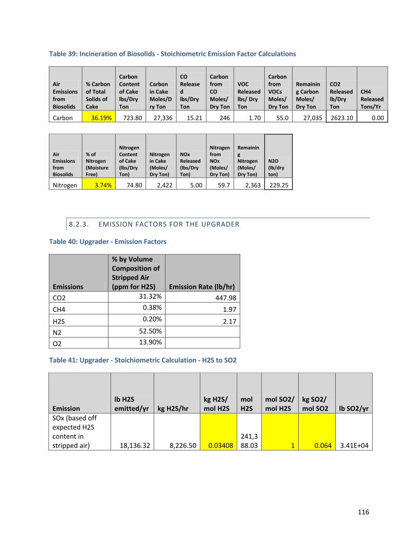
116
Table 39: Incineration of Biosolids - Stoichiometric Emission Factor Calculations
Air Emissions from Biosolids
% Carbon of Total Solids of Cake
Carbon Content of Cake lbs/Dry Ton
Carbon in Cake Moles/Dry Ton
CO Released lbs/Dry Ton
Carbon from CO Moles/ Dry Ton
VOC Released lbs/ Dry Ton
Carbon from VOCs Moles/ Dry Ton
Remaining Carbon Moles/ Dry Ton
CO2 Released lb/Dry Ton
CH4 Released Tons/Yr
Carbon 36.19% 723.80 27,336 15.21 246 1.70 55.0 27,035 2623.10 0.00
Air Emissions from Biosolids
% of Nitrogen (Moisture Free)
Nitrogen Content of Cake (lbs/Dry Ton)
Nitrogen in Cake (Moles/ Dry Ton)
NOx Released (lbs/Dry Ton)
Nitrogen from NOx (Moles/ Dry Ton)
Remaining Nitrogen (Moles/ Dry Ton)
N2O (lb/dry ton)
Nitrogen 3.74% 74.80 2,422 5.00 59.7 2,363 229.25
8.2.3. EMISSION FACTORS FOR THE UPGRADER
Table 40: Upgrader - Emission Factors
Emissions
% by Volume Composition of Stripped Air (ppm for H2S) Emission Rate (lb/hr)
CO2 31.32% 447.98 CH4 0.38% 1.97
H2S 0.20% 2.17 N2 52.50% O2 13.90%
Table 41: Upgrader - Stoichiometric Calculation - H2S to SO2
Emission lb H2S emitted/yr kg H2S/hr
kg H2S/ mol H2S
mol H2S
mol SO2/ mol H2S
kg SO2/ mol SO2 lb SO2/yr
SOx (based off expected H2S content in stripped air) 18,136.32 8,226.50 0.03408
241,388.03 1 0.064 3.41E+04
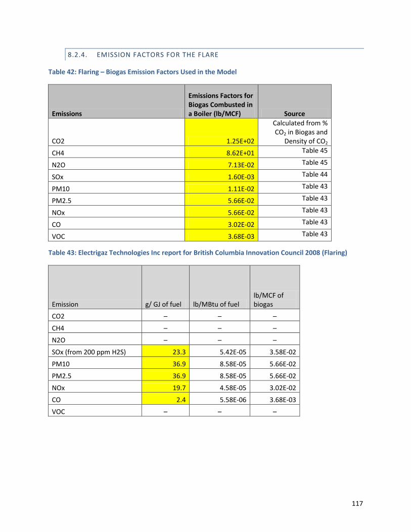
117
8.2.4. EMISSION FACTORS FOR THE FLARE
Table 42: Flaring – Biogas Emission Factors Used in the Model
Emissions
Emissions Factors for Biogas Combusted in a Boiler (lb/MCF) Source
CO2 1.25E+02
Calculated from % CO2 in Biogas and
Density of CO2
CH4 8.62E+01 Table 45
N2O 7.13E-02 Table 45
SOx 1.60E-03 Table 44
PM10 1.11E-02 Table 43
PM2.5 5.66E-02 Table 43
NOx 5.66E-02 Table 43
CO 3.02E-02 Table 43
VOC 3.68E-03 Table 43
Table 43: Electrigaz Technologies Inc report for British Columbia Innovation Council 2008 (Flaring)
Emission g/ GJ of fuel lb/MBtu of fuel lb/MCF of biogas
CO2 – – –
CH4 – – –
N2O – – –
SOx (from 200 ppm H2S) 23.3 5.42E-05 3.58E-02
PM10 36.9 8.58E-05 5.66E-02
PM2.5 36.9 8.58E-05 5.66E-02
NOx 19.7 4.58E-05 3.02E-02
CO 2.4 5.58E-06 3.68E-03
VOC – – –

118
Table 44: Stoichiometric Calculation (Flaring)
Emission % H2S of biogas
kg H2S/ MCF of biogas
kg H2S/ mol H2S
mol H2S
mol SO2/ mol H2S
kg SO2/ mol SO2
lb SO2/ MCF biogas
SOx (based off reported H2S content in biogas) 0.0068% 0.00268 0.03408 0.0787 1 0.064 0.0111
Table 45: GREET1_2011 Emission Factors for Natural Gas Flaring in Oil Field
Emission g/mmBtu of fuel lb/MBtu of fuel
lb/MCF of biogas
lb/MCF of nat gas
CO2 5.92E+04 1.31E-01 8.62E+01 1.31E+02
CH4 4.90E+01 1.08E-04 7.13E-02 1.08E-01
N2O 1.10E+00 2.43E-06 1.60E-03 2.43E-03
SOx 2.69E-01 5.93E-07 3.91E-04 5.93E-04
PM10 3.70E+00 8.16E-06 5.38E-03 8.16E-03
PM2.5 3.70E+00 8.16E-06 5.38E-03 8.16E-03
NOx 4.89E+01 1.08E-04 7.12E-02 1.08E-01
CO 2.60E+01 5.73E-05 3.78E-02 5.73E-02
VOC 2.50E+00 5.51E-06 3.64E-03 5.51E-03
8.2.5. EMISSIONS FACTORS FOR THE GENERATOR
Table 46. Generator – Biogas Emission Factors Used in the Model
Combustion Emissions
Emissions for Biogas Combusted in the Generator (lb/MCF) Source
CO2 1.14E+02 Table 49 CH4 1.97E-01 Table 47 N2O 7.68E-04 Table 48 SOx 1.11E-02 Table 49 PM10 6.92E-04 Table 48
PM2.5 3.16E-04 Table 48 NOx 2.17E-02 Table 47 CO 1.09E-01 Table 47 VOC 3.52E-02 Table 47
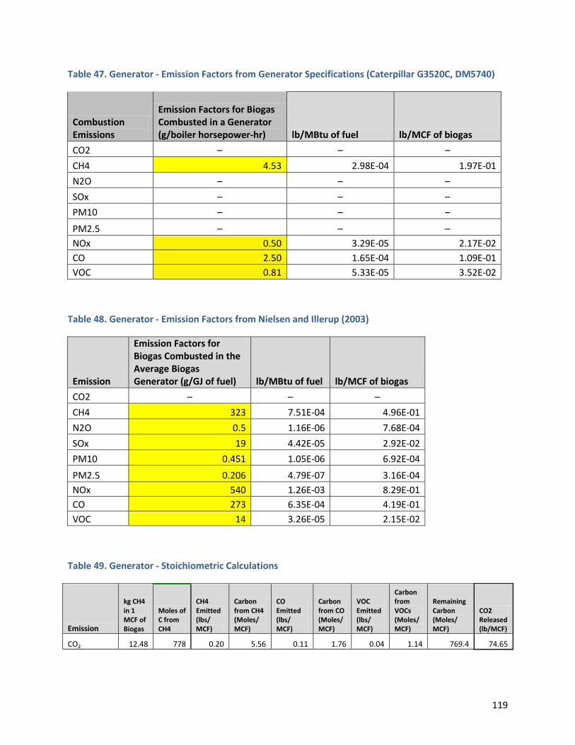
119
Table 47. Generator - Emission Factors from Generator Specifications (Caterpillar G3520C, DM5740)
Combustion Emissions
Emission Factors for Biogas Combusted in a Generator (g/boiler horsepower-hr) lb/MBtu of fuel lb/MCF of biogas
CO2 – – – CH4 4.53 2.98E-04 1.97E-01 N2O – – – SOx – – – PM10 – – –
PM2.5 – – – NOx 0.50 3.29E-05 2.17E-02 CO 2.50 1.65E-04 1.09E-01 VOC 0.81 5.33E-05 3.52E-02
Table 48. Generator - Emission Factors from Nielsen and Illerup (2003)
Emission
Emission Factors for Biogas Combusted in the Average Biogas Generator (g/GJ of fuel) lb/MBtu of fuel lb/MCF of biogas
CO2 – – – CH4 323 7.51E-04 4.96E-01 N2O 0.5 1.16E-06 7.68E-04 SOx 19 4.42E-05 2.92E-02 PM10 0.451 1.05E-06 6.92E-04
PM2.5 0.206 4.79E-07 3.16E-04 NOx 540 1.26E-03 8.29E-01 CO 273 6.35E-04 4.19E-01 VOC 14 3.26E-05 2.15E-02
Table 49. Generator - Stoichiometric Calculations
Emission
kg CH4 in 1 MCF of Biogas
Moles of C from CH4
CH4 Emitted (lbs/ MCF)
Carbon from CH4 (Moles/ MCF)
CO Emitted (lbs/ MCF)
Carbon from CO (Moles/ MCF)
VOC Emitted (lbs/ MCF)
Carbon from VOCs (Moles/ MCF)
Remaining Carbon (Moles/ MCF)
CO2 Released (lb/MCF)
CO2 12.48 778 0.20 5.56 0.11 1.76 0.04 1.14 769.4 74.65

120
Emission
% H2S of biogas
kg H2S/ MCF of biogas
kg H2S/ mol H2S mol H2S
mol SO2/ mol H2S
kg SO2/ mol SO2
lb SO2/ MCF biogas
SOx (based off reported H2S content in biogas)
0.0068%
0.00268 0.03408 0.0787 1 0.064
1.11E-02
8.2.6. EMISSION FACTORS FOR THE MICHIGAN ELECTRICITY GRID
Table 50: Electricity Grid - Emission Factors Used in the Model
Emissions for Primary Energy Combustion for Electricity Lb/ kWh Source
CO2 1.65111 eGRID2010 Version 1.1 Year 2007 GHG Annual Output Emission Rates
CH4 3.26E-05 eGRID2010 Version 1.1 Year 2007 GHG Annual Output Emission Rates
N2O 2.78E-05 eGRID2010 Version 1.1 Year 2007 GHG Annual Output Emission Rates
SO2 7.24E-03 eGRID2010 Version 1.1 Year 2007 GHG Annual Output Emission Rates
NOx 2.30E-03 eGRID2010 Version 1.1 Year 2007 GHG Annual Output Emission Rates

121
8.3. APPENDIX 3: EQUIPMENT AND ELECTRICITY USE TABLES
P-101 P-702 P-701
Date
Accumulated Dry Tons of Sludge
Adjusted Elapsed kWh Date
Accumulated Dry Tons of Sludge
Adjusted Elapsed kWh Date
Accumulated Dry Tons of Sludge
Adjusted Elapsed kWh
11/18/2011 0 0 11/28/2011 0 0 11/18/2011 0 011/21/2011 31.2522685 9.4 12/5/2011 104.2026286 1477 11/21/2011 31.2522685 379.07206411/28/2011 77.66292734 9.6 12/12/2011 197.4925371 3316 11/28/2011 77.66292734 1225.493248
12/5/2011 181.8655559 10.6 12/19/2011 255.2801127 7259 12/5/2011 181.8655559 2097.87827212/12/2011 275.1554645 10.6 12/26/2011 312.7921222 9253 12/12/2011 275.1554645 2913.14284812/19/2011 332.9430401 33.5 1/13/2012 399.5252441 13691 12/19/2011 332.9430401 3790.72064
1/20/2012 451.2212353 15577 12/26/2011 390.4550496 4631.9490561/13/2012 477.1881714 6371.5263361/20/2012 528.8841627 7223.140288
P-512 P-510 P-511
Date
Accumulated Dry Tons of Sludge
Adjusted Elapsed kWh Date
Accumulated Dry Tons of Sludge
Adjusted Elapsed kWh Date
Accumulated Dry Tons of Sludge
Adjusted Elapsed kWh
11/18/2011 0 0 11/18/2011 0 0 11/18/2011 0 011/21/2011 31.2522685 181.48392 11/21/2011 31.2522685 31.2522685 11/21/2011 31.2522685 90511/28/2011 77.66292734 592.34335 11/28/2011 77.66292734 77.66292734 11/28/2011 77.66292734 3028
12/5/2011 181.8655559 1015.80583 12/5/2011 181.8655559 181.8655559 12/5/2011 181.8655559 514812/12/2011 275.1554645 1411.5416 12/12/2011 275.1554645 275.1554645 12/12/2011 275.1554645 727712/19/2011 332.9430401 1837.52469 12/19/2011 332.9430401 332.9430401 12/19/2011 332.9430401 939212/26/2011 390.4550496 2248.38412 12/26/2011 390.4550496 11509
1/13/2012 477.1881714 3065.06176 1/13/2012 477.1881714 169911/20/2012 528.8841627 3478.4418 1/20/2012 528.8841627 18810
FA-610 FA-620 P-502
Date
Accumulated Dry Tons of Sludge
Adjusted Elapsed kWh Date
Accumulated Dry Tons of Sludge
Adjusted Elapsed kWh Date
Accumulated Dry Tons of Sludge
Adjusted Elapsed kWh
11/18/2011 0 0 11/18/2011 0 0 11/18/2011 0 011/21/2011 31.2522685 184.99236 11/21/2011 31.2522685 152.618697 11/21/2011 31.2522685 20.711/28/2011 77.66292734 332.986248 11/28/2011 77.66292734 776.967912 11/28/2011 77.66292734 24.1
12/5/2011 181.8655559 961.960272 12/5/2011 181.8655559 924.9618 12/5/2011 181.8655559 5012/12/2011 275.1554645 1498.438116 12/12/2011 275.1554645 1160.827059 12/12/2011 275.1554645 91.912/19/2011 332.9430401 1646.432004 12/19/2011 332.9430401 1799.050701 12/19/2011 332.9430401 125.212/26/2011 390.4550496 2275.406028 12/26/2011 390.4550496 1947.044589 12/26/2011 390.4550496 162.6
1/13/2012 477.1881714 3352.986525 1/13/2012 477.1881714 2876.631198 1/13/2012 477.1881714 213.11/20/2012 528.8841627 3524.104458 1/20/2012 528.8841627 3463.981941 1/20/2012 528.8841627 245.1
AG-610 AG-620 P-601
Date
Accumulated Dry Tons of Sludge
Adjusted Elapsed kWh Date
Accumulated Dry Tons of Sludge
Adjusted Elapsed kWh Date
Accumulated Dry Tons of Sludge
Adjusted Elapsed kWh
11/21/2011 0 0 11/21/2011 0 0 11/28/2011 0 011/28/2011 124.0735862 100 11/28/2011 46.41065885 116.305824 12/5/2011 104.2026286 54.2
12/5/2011 228.2762148 180 12/5/2011 150.6132874 174.458736 12/12/2011 197.4925371 90.812/12/2011 321.5661233 293.83704 12/12/2011 243.903196 414.339498 12/19/2011 255.2801127 90.812/19/2011 379.3536989 500.922192 12/19/2011 301.6907716 617.87469 12/26/2011 312.7921222 131.7
12/26/2011 359.2027811 811.71773 1/13/2012 399.5252441 198.41/13/2012 445.9359029 1398.092926 1/20/2012 451.2212353 199.4

122
P-602 CD-901 Drum Motor CD-901 Scroll Motor
Date
Accumulated Dry Tons of Sludge
Adjusted Elapsed kWh Date
Accumulated Dry Tons of Sludge
Adjusted Elapsed kWh Date
Accumulated Dry Tons of Sludge
Adjusted Elapsed kWh
11/21/2011 0 0 11/18/2011 0 0 11/18/2011 0 011/28/2011 46.41065885 43.7 11/21/2011 31.2522685 31.2522685 11/21/2011 31.2522685 0.023
12/5/2011 150.6132874 43.7 11/28/2011 77.66292734 77.66292734 11/28/2011 77.66292734 0.03412/12/2011 243.903196 53.8 12/5/2011 181.8655559 181.8655559 12/5/2011 181.8655559 0.08312/19/2011 301.6907716 106.8 12/12/2011 275.1554645 0.14312/26/2011 359.2027811 106.8 12/19/2011 332.9430401 0.235
1/13/2012 445.9359029 160.4 12/26/2011 390.4550496 0.2881/20/2012 497.6318942 206.1 1/13/2012 477.1881714 0.494
1/20/2012 528.8841627 0.562
CD-902 Drum Motor CD-902 Scroll Motor C-1000
Date
Accumulated Dry Tons of Sludge
Adjusted Elapsed kWh Date
Accumulated Dry Tons of Sludge
Adjusted Elapsed kWh Date
Accumulated Dry Tons of Sludge
Adjusted Elapsed kWh
11/18/2011 0 0 11/18/2011 0 0 11/18/2011 0 011/21/2011 31.2522685 0.13 11/21/2011 31.2522685 0.026 11/21/2011 31.2522685 57.2422411/28/2011 77.66292734 0.3 11/28/2011 77.66292734 0.04 11/28/2011 77.66292734 165.644732
12/5/2011 181.8655559 0.3 12/5/2011 181.8655559 0.067 12/5/2011 181.8655559 289.07331212/12/2011 275.1554645 2.3 12/12/2011 275.1554645 0.172 12/12/2011 275.1554645 424.30810412/19/2011 332.9430401 4.82 12/19/2011 332.9430401 0.305 12/19/2011 332.9430401 547.73668412/26/2011 390.4550496 6.67 12/26/2011 390.4550496 0.427 12/26/2011 390.4550496 675.637314
1/13/2012 477.1881714 9.67 1/13/2012 477.1881714 0.631 1/13/2012 477.1881714 763.1106121/20/2012 528.8841627 10.8 1/20/2012 528.8841627 0.714
Boiler P-100 East Mixing Pump
Date
Accumulated Dry Tons of Sludge
Adjusted Elapsed kWh Date
Accumulated Dry Tons of Sludge
Adjusted Elapsed kWh Date
Accumulated Dry Tons of Sludge
Adjusted Elapsed kWh
11/18/2011 0 0 7/24/2011 0 0 11/28/2011 0 011/21/2011 31.2522685 43.8982656 8/1/2011 326012 22.2 12/5/2011 104.2026286 147711/28/2011 77.66292734 122.2635288 8/3/2011 407525 59.6 12/12/2011 197.4925371 3316
12/5/2011 181.8655559 212.4607464 8/15/2011 896687 59.6 12/19/2011 255.2801127 725912/12/2011 275.1554645 313.4610528 8/19/2011 1059773 96.3 12/26/2011 312.7921222 925312/19/2011 332.9430401 403.3153152 8/26/2011 1345212 174.6 1/13/2012 399.5252441 1369112/26/2011 390.4550496 497.4565176 9/3/2011 1671488 216.6 1/20/2012 451.2212353 15577
1/13/2012 477.1881714 680.766072 9/9/2011 1916237 216.61/20/2012 528.8841627 789.9973032
P-503 P-501
Date
Accumulated Dry Tons of Sludge
Adjusted Elapsed kWh Date
Accumulated Dry Tons of Sludge
Adjusted Elapsed kWh
10/14/2011 0 0 11/18/2011 0 010/21/2011 59.15758407 82.9362 11/21/2011 31.2522685 31.610/28/2011 113.7432594 414.681 11/28/2011 77.66292734 92.5
11/4/2011 162.1355539 559.81935 12/5/2011 181.8655559 13912/12/2011 275.1554645 172.312/19/2011 332.9430401 217.412/26/2011 390.4550496 254.5
1/13/2012 477.1881714 353.21/20/2012 528.8841627 402.2

123
8.4. APPENDIX 4: IMPACT CHARACTERIZATION FACTORS
Midpoints CO2 CH4 N2O SOx NOx CO PM
(10) PM
(2.5) VOC NH3 Lead Global Warming Potential (lb CO2eq/lb of Emission) 1 25 298 - - - - - - - - Acidification Potential (moles H+/lb of Emission) - - -
23.0864
23.0227 - - - -
43.4045 -
Smog Formation Potential (lb O3 eq/lb of Emission) -
0.0144 - -
20.8170
0.0556 - -
3.5954 - -
8.5. APPENDIX 5: SENSITIVITY ANALYSES
Figure 40. Sensitivity Analysis of Acidification Potential in Current Operations

124
Figure 41. Sensitivity Analysis of Smog Formation Potential in Current Operations
Figure 42. Sensitivity Analysis of Acidification Potential in Fully Operational with Generator

125
Figure 43. Sensitivity Analysis of Smog Formation Potential in Fully Operational with Generator