LIENS Code de la Propriété Intellectuelle. articles L 122....
195
AVERTISSEMENT Ce document est le fruit d'un long travail approuvé par le jury de soutenance et mis à disposition de l'ensemble de la communauté universitaire élargie. Il est soumis à la propriété intellectuelle de l'auteur. Ceci implique une obligation de citation et de référencement lors de l’utilisation de ce document. D'autre part, toute contrefaçon, plagiat, reproduction illicite encourt une poursuite pénale. Contact : [email protected] LIENS Code de la Propriété Intellectuelle. articles L 122. 4 Code de la Propriété Intellectuelle. articles L 335.2- L 335.10 http://www.cfcopies.com/V2/leg/leg_droi.php http://www.culture.gouv.fr/culture/infos-pratiques/droits/protection.htm
Transcript of LIENS Code de la Propriété Intellectuelle. articles L 122....

AVERTISSEMENT
Ce document est le fruit d'un long travail approuvé par le jury de soutenance et mis à disposition de l'ensemble de la communauté universitaire élargie. Il est soumis à la propriété intellectuelle de l'auteur. Ceci implique une obligation de citation et de référencement lors de l’utilisation de ce document. D'autre part, toute contrefaçon, plagiat, reproduction illicite encourt une poursuite pénale. Contact : [email protected]
LIENS Code de la Propriété Intellectuelle. articles L 122. 4 Code de la Propriété Intellectuelle. articles L 335.2- L 335.10 http://www.cfcopies.com/V2/leg/leg_droi.php http://www.culture.gouv.fr/culture/infos-pratiques/droits/protection.htm

Ecole doctorale IAEM Lorraine
Modeles de Minimisation d’Energies Discretespour la Cartographie Cystoscopique
THESE
presentee et soutenue publiquement le 9 juillet 2013
pour l’obtention du
Doctorat de l’Universite de Lorraine
Mention : Automatique, Traitement du Signal et des Images, Genie Informatique
par
Thomas WEIBEL
Composition du jury :
President : Jean-Marc CHASSERY DR CNRS, GIPSA-Lab, Grenoble.
Rapporteurs : Fabrice HEITZ PU, Universite de Strasbourg, ICube.
Joachim OHSER PU, Hochschule Darmstadt, Allemagne.
Examinateurs : Francois GUILLEMIN PUPH, Universite de Lorraine,CRAN/ICL, Nancy.
Ronald ROSCH PhD, Fraunhofer ITWM,Kaiserslautern, Allemagne.
Directeur de these : Christian DAUL PU, Universite de Lorraine, CRAN, Nancy.
Co-Directeur de these : Didier WOLF PU, Universite de Lorraine, CRAN, Nancy.
Centre de Recherche en Automatique de NancyUMR 7039 Universite de Lorraine - CNRS
2, avenue de la foret de Haye 54516 Vandœuvre-les-NancyTel : +33 (0)3 83 59 59 59 Fax : +33 (0)3 83 59 56 44


To Michael Jordan. And Henrike.

Acknowledgements
I owe the most sincere and earnest thankfulness to my supervisor Christian Daul.
Without his constant support and guidance, this thesis would not have been possible.
I have enjoyed each and every of our discussions in the last three years. His passion
for research and his work ethics are admirable, and by keeping his sense of humour
whenever I had lost mine, he always made me retain focus. I sincerely hope that we
can continue our fruitful collaboration, professionally and more so personally.
I would also like to express my gratitude towards my co-supervisor Didier Wolf,
whose experience in applied research helped me to look at problems from a different
point of view and shape the final version of this manuscript.
Furthermore, I would like to thank Joachim Ohser and Fabrice Heitz for agreeing
to review this manuscript. Not only did their reports provide critical remarks that
helped to improve the final version. But more importantly, their kind and positive
feedback reassured me that the last three years were not spend in vain.
I would also like to thank Jean-Marc Chassery for acting as chairman of the jury
and for valuable discussion during the defense.
In particular, I owe gratitude to Francois Guillemin, who initiated this project
several years ago. His medical expertise and suggestions throughout the last three
years were priceless and provided tremendous help in understanding the important
aspects from a medical point of view.
Of course I would also like to thank the image processing department of the Fraun-
hofer ITWM for both funding as well as a scientifically fruitful and most pleasant
working environment. Particular thanks go to Ronald Rosch and Markus Rauhut
for giving me the opportunity to pursue my academic endeavours, to Behrang Shafei
and Henrike Stephani for proofreading, and to Falco Hirschenberger for always com-
ing up with elegant solutions to computer engineering related problems.
I thank the staff of CINVESTAV, in particular Dr. Lorenzo Leija Salas and Dr.
Arturo Vera Hernandez, and the program ECOS for financing my stay in Mexico.
Last, but not least, I would like to thank my parents, my sister, and my grandparents
for their constant support from the very beginning, and especially to Henrike for
always being there for me. I cannot thank her enough for sticking with me and
enduring all those moods. This one is also for you guys.


Contents
Introduction ix
1 Cystoscopic Cartography 1
1.1 Medical Context . . . . . . . . . . . . . . . . . . . . . . . . . . . . . . . . . . . . 1
1.1.1 Bladder Cancer . . . . . . . . . . . . . . . . . . . . . . . . . . . . . . . . . 1
1.1.2 Cystoscopic Examination . . . . . . . . . . . . . . . . . . . . . . . . . . . 1
1.2 Image Mosaicing . . . . . . . . . . . . . . . . . . . . . . . . . . . . . . . . . . . . 6
1.2.1 General Applications of Image Mosaicing . . . . . . . . . . . . . . . . . . 7
1.2.2 Medical Applications . . . . . . . . . . . . . . . . . . . . . . . . . . . . . . 7
1.3 2D Endoscopic Cartography . . . . . . . . . . . . . . . . . . . . . . . . . . . . . . 8
1.3.1 Pre-Processing . . . . . . . . . . . . . . . . . . . . . . . . . . . . . . . . . 10
1.3.2 Geometry of Cystoscopic Image Acquisition Systems . . . . . . . . . . . . 13
1.3.3 Registration of Cystoscopic Images . . . . . . . . . . . . . . . . . . . . . . 16
1.3.4 Map Compositing . . . . . . . . . . . . . . . . . . . . . . . . . . . . . . . 19
1.3.5 First Assessment of Existing Endoscopic Cartography Approaches . . . . 22
1.4 3D Endoscopic Cartography . . . . . . . . . . . . . . . . . . . . . . . . . . . . . . 22
1.4.1 2D Endoscopic Cartography with 3D a priori Knowledge . . . . . . . . . . 23
1.4.2 3D Endoscopic Cartography . . . . . . . . . . . . . . . . . . . . . . . . . . 24
1.4.3 3D Endoscopes . . . . . . . . . . . . . . . . . . . . . . . . . . . . . . . . . 25
1.4.4 First Assessment of Existing 3D Endoscopic Cartography Approaches . . 26
1.5 Objectives of the thesis . . . . . . . . . . . . . . . . . . . . . . . . . . . . . . . . 26
1.5.1 Scientific Objectives . . . . . . . . . . . . . . . . . . . . . . . . . . . . . . 26
1.5.2 Medical Interest and Time Constraints . . . . . . . . . . . . . . . . . . . 29
1.5.3 Global Approach: Discrete Energy Minimization as a Framework for Cys-
toscopic Cartography Algorithms . . . . . . . . . . . . . . . . . . . . . . . 29
v

CONTENTS
2 Graph-Cut Optimization 31
2.1 Discrete Energy Minimization in Computer Vision . . . . . . . . . . . . . . . . . 31
2.1.1 Order and Interaction . . . . . . . . . . . . . . . . . . . . . . . . . . . . . 32
2.1.2 Markov Random Fields . . . . . . . . . . . . . . . . . . . . . . . . . . . . 32
2.2 Energy Minimization using Graph-Cuts . . . . . . . . . . . . . . . . . . . . . . . 33
2.2.1 The st-Mincut/ Maxflow Theorem . . . . . . . . . . . . . . . . . . . . . . 33
2.2.2 Graph-Cut Examples for Two-Label Problems . . . . . . . . . . . . . . . 39
2.2.3 Submodular and Non-Submodular Energy Functions . . . . . . . . . . . . 42
2.2.4 Higher-Order Energy Functions . . . . . . . . . . . . . . . . . . . . . . . . 44
2.3 Graph-Cuts for Multi-Label Problems . . . . . . . . . . . . . . . . . . . . . . . . 46
2.3.1 Move-Making Algorithms . . . . . . . . . . . . . . . . . . . . . . . . . . . 47
2.3.2 Transformation Methods . . . . . . . . . . . . . . . . . . . . . . . . . . . . 51
2.3.3 Example for Multi-Label Problems: Image De-Noising . . . . . . . . . . . 52
2.4 Graph-Cuts for Image Registration and Map Compositing . . . . . . . . . . . . . 56
2.4.1 Image Registration using Graph-Cuts . . . . . . . . . . . . . . . . . . . . 56
2.4.2 Map Compositing using Graph-Cuts . . . . . . . . . . . . . . . . . . . . . 58
2.5 Sparse Graph-Cuts for Cystoscopic Image Registration: a Proof of Concept . . . 60
2.5.1 Cystoscopic Image Registration Assessment . . . . . . . . . . . . . . . . . 60
2.5.2 Cystoscopic Image Registration using Standard Graph-Cuts . . . . . . . . 61
2.5.3 Sparse Graph-Cuts with Locally Refined Vertex and Edge Selection . . . 62
2.5.4 Initial Results . . . . . . . . . . . . . . . . . . . . . . . . . . . . . . . . . . 65
2.6 Conclusions . . . . . . . . . . . . . . . . . . . . . . . . . . . . . . . . . . . . . . . 66
3 2D Cartography 69
3.1 Problem Description and Chapter Overview . . . . . . . . . . . . . . . . . . . . . 69
3.2 Global Map Correction . . . . . . . . . . . . . . . . . . . . . . . . . . . . . . . . . 72
3.2.1 Detecting Additional Image Pairs . . . . . . . . . . . . . . . . . . . . . . . 73
3.2.2 Bundle Adjustment . . . . . . . . . . . . . . . . . . . . . . . . . . . . . . 75
3.3 Image Registration using Perspective-Invariant Cost Functions . . . . . . . . . . 76
3.3.1 Data Term . . . . . . . . . . . . . . . . . . . . . . . . . . . . . . . . . . . 77
3.3.2 Regularization Term . . . . . . . . . . . . . . . . . . . . . . . . . . . . . . 79
3.3.3 Cost Function and Coarse-To-Fine Minimization Scheme . . . . . . . . . . 81
3.4 Contrast-Enhancing Map Compositing . . . . . . . . . . . . . . . . . . . . . . . . 85
3.4.1 Seam Localization . . . . . . . . . . . . . . . . . . . . . . . . . . . . . . . 86
3.4.2 Exposure and Vignetting Correction . . . . . . . . . . . . . . . . . . . . . 88
3.5 Results . . . . . . . . . . . . . . . . . . . . . . . . . . . . . . . . . . . . . . . . . . 89
3.5.1 Quantitative Evaluation on Phantom Data . . . . . . . . . . . . . . . . . 90
3.5.2 Qualitative Evaluation on Clinical Data . . . . . . . . . . . . . . . . . . . 94
3.5.3 Results on Traditional Applications . . . . . . . . . . . . . . . . . . . . . 106
3.6 Discussion and Perspectives . . . . . . . . . . . . . . . . . . . . . . . . . . . . . . 109
vi

CONTENTS
3.6.1 Practical and Scientific Contributions . . . . . . . . . . . . . . . . . . . . 109
3.6.2 Limits of the Methods and Perspectives . . . . . . . . . . . . . . . . . . . 111
3.6.3 Publications . . . . . . . . . . . . . . . . . . . . . . . . . . . . . . . . . . . 112
4 3D Cartography: a Proof of Concept 113
4.1 Introduction and Chapter Overview . . . . . . . . . . . . . . . . . . . . . . . . . 113
4.1.1 Motivation and Projection Geometry . . . . . . . . . . . . . . . . . . . . . 114
4.1.2 Choice of 3D Map Reconstruction Principle . . . . . . . . . . . . . . . . . 116
4.2 Data Acquisition . . . . . . . . . . . . . . . . . . . . . . . . . . . . . . . . . . . . 117
4.2.1 Laser-Based Cystoscope Prototype . . . . . . . . . . . . . . . . . . . . . . 118
4.2.2 Time-of-Flight Prototype . . . . . . . . . . . . . . . . . . . . . . . . . . . 119
4.2.3 RGB-Depth Cameras . . . . . . . . . . . . . . . . . . . . . . . . . . . . . 121
4.3 3D Cartography Approach . . . . . . . . . . . . . . . . . . . . . . . . . . . . . . . 122
4.3.1 Overview of the 3D Cartography Steps . . . . . . . . . . . . . . . . . . . . 122
4.3.2 Three-Dimensional Data Registration . . . . . . . . . . . . . . . . . . . . 123
4.3.3 Global Map Correction . . . . . . . . . . . . . . . . . . . . . . . . . . . . 126
4.3.4 Contrast-Enhanced Surface Compositing . . . . . . . . . . . . . . . . . . . 127
4.4 Results . . . . . . . . . . . . . . . . . . . . . . . . . . . . . . . . . . . . . . . . . . 132
4.4.1 2D and 3D Registration Robustness and Accuracy on a Simulated Phantom133
4.4.2 Global Map Reconstruction Accuracy . . . . . . . . . . . . . . . . . . . . 139
4.4.3 Surface Compositing . . . . . . . . . . . . . . . . . . . . . . . . . . . . . . 148
4.5 Conclusions and Perspectives . . . . . . . . . . . . . . . . . . . . . . . . . . . . . 153
4.5.1 Main Scientific Contributions . . . . . . . . . . . . . . . . . . . . . . . . . 153
4.5.2 Limits and Perspectives . . . . . . . . . . . . . . . . . . . . . . . . . . . . 154
Conclusion 157
References 161
vii

CONTENTS
viii

Introduction
This thesis was written at the CRAN laboratory (Centre de Recherche en Automatique de
Nancy, UMR 7039 CNRS/Universite de Lorraine) in the department SBS (Sante-Biologie-
Signal). The thesis framework is a scientific cooperation between the CRAN and the department
of image processing at the Fraunhofer Institute for Industrial Mathematics (ITWM), which also
provided the financial support. One field of research within the SBS department aims at fa-
cilitating bladder cancer diagnosis. The thesis is situated in this context. Medical expertise
and data is supplied by Prof. Francois Guillemin from the ICL (Institut de Cancerologie de
Lorraine), which is a comprehensive cancer center located in Nancy.
The reference clinical procedure for bladder cancer diagnosis is cystoscopy. The purpose
of such an examination is to visually explore the internal epithelial wall of the human bladder
using a cystoscope (a rigid or flexible endoscope specifically designed for bladder examination).
The organ is filled with an isotonic saline solution during the examination, which temporarily
rigidifies the bladder’s internal walls. The cystoscope is then inserted through the urethra, and
the surface of the epithelium is systematically scanned for cancerous or other lesions. These can
then be surgically removed using tools inserted through an operative channel of the instrument.
The surface is illuminated using either white or fluorescence light. On the one hand, the white
light modality corresponds to the standard and reference modality, which results in a natural
appearance of the epithelium. The fluorescence light modality, on the other hand, can be used
after injection of a marker substance to facilitate early cancer detection, at the expense of a
natural epithelium appearance. For these reasons, fluorescence illumination is never used solely.
Clinicians (urologists and surgeons) perform their diagnosis by observing a video-sequence on
a monitor.
The main limitation of a cystoscopic examination is the small field of view (FOV) of cys-
toscopes, which complicates endoscope navigation and scene interpretation for the clinicians.
Furthermore, bladder tumours, which appear on the first skin layers, are often multi-focal (they
appear as multiple spots on the epithelial surface). Due to the small FOV of the cystoscope, it
is therefore not possible to observe, in one single image, the entire spatial distribution of lesions
(tumours, scars, etc.), as well as their localization with respect to anatomical landmarks (such
ix
Introduction
as the ureters or air bubbles). Because it is difficult to interpret the acquired data at a later
point without the physical feedback of navigating the cystoscope, video-sequences are currently
not archived for patient follow-up. Instead, regions of interest are annotated on an anatomi-
cal sketch of the bladder, and print-outs corresponding to these regions are archived with this
sketch. Such a print out also shows a surface area limited by the FOV of the images. The
archived data (small FOV and no anatomical landmarks visible) does not facilitate diagnosis,
lesion follow-up preparations, and treatment traceability.
These limitations can be overcome with the aid of two- and three-dimensional cartography al-
gorithms. Indeed, large FOV maps, constructed with the images of cystoscopic video-sequences,
allow for archiving the recorded sequence in an intuitive format, i.e. a single two-dimensional
panoramic image or a three-dimensional textured mesh. Such maps (also referred to as mosaics)
can be used to compare lesion evolution side-by-side, while greatly reducing data redundancy.
During a follow-up examination, these maps also facilitate navigation inside the organ (both
lesions and anatomical landmarks are visible) and minimize the risk of missing regions of in-
terest observed in a previous examination. They also enable a second diagnosis (after the
examination) by the clinician who acquired the data or by other clinicians.
Two-dimensional cartography algorithms allow for constructing large FOV panoramic im-
ages from conventional cystoscopic video-sequences. However, due to the non-planar shape of
the bladder and the varying cystoscope viewpoints during the examination, the resolution of
the panoramic image is often severely “distorted” for larger FOVs. Techniques used in classical
panoramic imaging to overcome this problem (e.g. by using spherical coordinates) do not apply
in this context, as they require a stationary camera rotating around its optical center. Further-
more, clinicians are still required to mentally project the two-dimensional map onto the organ’s
three-dimensional shape. Both difficulties can be overcome with the aid of three-dimensional
cartography algorithms. These allow to reconstruct a textured mesh of the observed part of
the bladder, whose resolution depends only on the distance between cystoscope and epithelium.
However, the downside of three-dimensional cartography is that the bladder’s poor local depth
variation requires modified instruments to robustly construct three-dimensional maps.
The general aim of this thesis is to design and implement both two- and three-dimensional
cartography algorithms in order to facilitate bladder lesion diagnosis and follow-up. Such al-
gorithms consist of several steps. Overlapping images of the video-sequence must be registered
(superimposed) in a robust and accurate fashion and then placed into a common coordinate sys-
tem. Crossing cystoscope trajectories create multiple overlapping map parts, requiring global
optimization to achieve coherent data superimposition. Finally, once the transformation pa-
rameters are estimated, the texture for each pixel/face in the map must be selected from the
redundant data available in the video-sequence.
Previous contributions showed the feasibility of two-dimensional cartography of hollow or-
gans. However, these methods work only robustly and reliably with regard to the registration
of consecutive image pairs, which are normally related by small viewpoint changes. This is a
x

Introduction
strong limitation, as small registration errors (between consecutive image pairs) accumulate to
larger global cartography errors. This leads to visible misalignments (texture discontinuities)
between non-consecutive images when the cystoscope returns to a previously visited location
(i.e. for crossing endoscope trajectories or loops). Robust and accurate registration of these
non-consecutive image pairs is most often not possible with existing contributions, as the images
are related by large viewpoint differences. Moreover, up to this point, no method to automati-
cally detect and correct accumulated errors for the cartography of cystoscopic video-sequences
has been proposed. Therefore, previous contributions only presented “strip”-shaped maps with
a large FOV in one main direction. One aim of this thesis is to design and implement an
algorithm that automatically detects and corrects accumulated errors. This requirement im-
mediately leads to another aim: the development of a registration algorithm that is able to
systematically register images related by larger viewpoint changes. Reaching both aims will
allow for constructing fully large FOV maps (e.g. multiple overlapping strips).
Once the transformations that place each image of the sequence into the common map co-
ordinate system have been computed, panoramic images without strong texture discontinuities
can be constructed. However, small bladder texture misalignments (for instance due to tem-
poral local bladder deformations) and visible color gradients (due to vignetting and different
exposure of the images) remain perceptible and must be corrected for a seamless and visually
coherent appearance. Additionally, many images suffer from motion blur and camera de-focus.
Previous contributions, based on (non-)linear interpolation, tend to produce blurry bladder
texture, as they do not consider the quality of the individual images. Hence, another aim of
the thesis is to correct small texture misalignments and exposure gradients without blending,
and to prefer well contrasted images over blurry data when available.
The global scientific aim of this thesis is to show the feasibility of discrete energy minimiza-
tion techniques in the context of cystoscopic cartography and to develop algorithms that solve
the goals formulated in the previous paragraphs. In particular, it should be shown that such
methods can be a robust and elegant approach for the core stages of the cartography pipeline.
Recent advances in this field (e.g. higher-order inference, minimization strategies) potentially
allow to achieve more accurate and robust results than those obtained with existing bladder
cartography approaches. Of particular interest are techniques based on the st-mincut/maxflow
theorem, which allow to solve discrete labeling problems using specifically constructed graphs.
Such algorithms, often referred to as graph-cuts in the computer vision context, have been
successfully applied to many image processing applications, such as image segmentation, image
de-noising, or the estimation of disparity and optical flow. Only a few contributions also ap-
ply these techniques to image registration and image compositing. However, these approaches
cannot be directly applied in the context of cystoscopic cartography due to the limitations
discussed previously.
Another aim of this thesis is to design the algorithms in such a way that they can be applied
to two-dimensional cartography and be extended to three-dimensional cartography. There, the
xi

Introduction
challenge is to find the geometric link between local coordinate systems, which correspond to
different viewpoints of the instrument. These links allow for reconstructing the cystoscope
trajectory and the three-dimensional shape of the epithelium. Only a few approaches can be
found in the literature concerned with three-dimensional cartography of endoscopic data. These
contributions are either based on a priori knowledge, active-stereo principles, structure from
motion, or external navigation systems. As will be discussed, the poor local geometry of the
bladder and the small FOV observed in each viewpoint impedes the use of these approaches
to robustly recover viewpoints and three-dimensional structure. It was however shown in a
previous thesis written at the CRAN laboratory, that an active-stereo-vision system, guided
by two-dimensional image registration, allows to recover the cystoscope trajectory and a set
of three-dimensional measurements on the epithelium. This approach is based on hypotheses
derived from two-dimensional cartography. However, these hypotheses do not hold in general
for arbitrary viewpoint changes in three-dimensional cartography. Consequently, the existing
approach is not able to register non-consecutive acquisitions. As is the case for previous contri-
butions to two-dimensional cartography, only “strip”-shaped three-dimensional bladder recon-
structions were presented. Furthermore, it was not shown how the (sparse) three-dimensional
bladder reconstruction can be textured using the images of the video-sequence. Therefore, the
last aim of this thesis is to show the feasibility of energy minimization techniques for three-
dimensional bladder reconstruction. Viewpoint estimation should not depend on 2D hypotheses
and arbitrary viewpoint links should be estimated robustly and accurately. Finally, a trian-
gulated mesh must be obtained from the reconstructed points. This mesh should be textured
from the available images, ensuring seamless alignment of vascular structures, while maximizing
contrast of the observed scene and removing any exposure related gradients.
To reach these goals, the thesis is structured as follows.
Chapter 1: Cystoscopic Cartography. This chapter first introduces the medical context
of the thesis. Then, previous contributions towards two- and three-dimensional endoscopic
cartography are discussed. A particular focus is laid on state-of-the-art techniques for bladder
cartography. Each step of the cartography pipeline is described, and advantages and drawbacks
of existing methods are discussed. The chapter concludes with a more detailed formulation of
the scientific and medical objectives of this thesis.
Chapter 2: Graph-Cut Optimization. The second chapter introduces the mathematical
and algorithmic framework of graph-based discrete energy minimization techniques. The de-
scribed discrete energy minimization principles and algorithms build the basis for the methods
proposed in Chapters 3 and 4. It is shown how energy functions whose variables may take
arbitrary values (such as displacement vectors in R2) can be minimized, and how higher-order
interaction between variables can be incorporated into a pairwise (graph-representable) form.
Then, previous applications of graph-cut approaches towards image registration and image
xii
Introduction
compositing are presented. The chapter concludes with a proposition of a first modification
of a reference graph-cut based image registration technique. A qualitative comparison with
state-of-the-art white light bladder image registration algorithms demonstrates the feasibility
of discrete energy minimization for the registration of video-sequences acquired in the white
light modality.
Chapter 3: 2D Cartography. In Chapter 3, a complete two-dimensional cartography
pipeline is presented. To overcome the limitations of existing state-of-the-art registration tech-
niques, higher-order potential functions are proposed. These allow to compute image similarity
and regularization costs invariantly of the underlying geometric transformations linking partly
overlapping small FOV images of the epithelium. The proposed cost functions allow to robustly
register both consecutive and non-consecutive image pairs of a video-sequence with high accu-
racy. The transformations of non-consecutive image pairs are are required to globally correct
accumulated errors between different trajectories. Furthermore, a technique to detect over-
lapping trajectories and to select a small subset of additional (non-consecutive) image pairs is
presented. It is then shown how the combined set of consecutive and non-consecutive transfor-
mation parameters can be used to globally optimize the placement of all images into a common
global coordinate system. Lastly, an energy minimization based map compositing algorithm is
proposed. The method allows to correct small remaining misalignments of vascular structures
in overlapping image regions in a first step, and at the same time maximizes the map’s texture
quality by favouring contrasted images over blurry ones. In a second step, exposure related
artefacts are removed without blurring or interpolation, and the corrected map retains both
contrast and hue of the original input images. Finally, the proposed methods are evaluated both
quantitatively and qualitatively on realistic phantom data as well as on clinical data acquired
at the ICL. Furthermore, results on non-medical applications, such as consumer photography
stitching and high-dynamic-range imaging, demonstrate that the proposed methods are also
applicable in more general scenarios.
Chapter 4: 3D Cartography. The last chapter describes extensions made to the algorithms
proposed in Chapter 3, which allow to construct three-dimensional large FOV texured meshes.
As previously discussed, the bladder’s three-dimensional structure cannot be robustly recon-
structed without modified cystoscopes. The results presented are a proof-of-concept, obtained
from realistic bladder phantoms and two cystoscope prototypes developed at the CRAN labora-
tory. It is shown that only minor modifications of the two-dimensional cartography algorithms
are necessary in order to construct large FOV textured meshes. Besides registration and global
map correction adaptation, the compositing algorithm is modified to work on triangular surface
meshes instead of a pixel level. This formulation allows to achieve the same goals as in two
dimensions, namely to maximize the contrast of the texture and remove exposure related arte-
facts. The results show the potential of the proposed methods on several acquisition scenarios,
including non-medical scenes captured with the Kinect sensor.
xiii

Introduction
xiv

Chapter 1
Cystoscopic Cartography
1.1 Medical Context
1.1.1 Bladder Cancer
Bladder cancer is the 7th most common type of cancer in the world (TP03), the fourth most
common malignant lesion among males in industrialized countries (Soc08), and the second most
common urinary disease. Ninety-five percent of bladder tumours originate on the first cell layers
of the epithelial surface of the internal bladder wall. Epithelial tumour tissue occurs when some
cells start to abnormally multiply (i.e. without control). Figure 1.1 illustrates the genesis of
epithelial tumours.
After bladder cancer detection, tests are necessary to check the lesions’ degree of evolution.
These tests are referred to as staging, and are helpful in guiding future treatment and follow-up.
Bladder cancer stages are classified using the TNM (primary Tumour, lymph Nodes, distinct
Metastasis) staging system. Figure 1.2 shows the major stages of primary tumours.
Research results suggest lifetime monitoring of patients after surgical removal of cancerous
tumours to avoid recurrence (HLCB+04).
1.1.2 Cystoscopic Examination
Since bladder lesions usually appear in an early stage on the internal epithelial surface, poten-
tial cancers can be visualized and detected with cameras. Bladder monitoring is conducted in a
cystoscopic examination, where a rigid or flexible cystoscope (an endoscope designed for bladder
examination), see Figures 1.3b-c, is inserted through the urethra into the bladder. The textured
epithelial surface of the bladder wall is classically visualized on a monitor (see Figure 1.3a).
During the examination, the bladder is filled with an isotonic solution, which temporarily in-
flates the bladder and limits bladder wall movements and shape changes. However, the bladder
1

1. CYSTOSCOPIC CARTOGRAPHY
Figure 1.1: Simplified representation of the different stages leading to bladder tumours. Thisillustration of the epithelial tissue evolution is taken from (HM07). (a) Mutation of a singlecell. (b) Abnormal augmentation of the number of cells and increasing cell size. (c) Abnormaldevelopment of the tissue (dysplasia). (d) Cancer in situ. (e) Propagation of the tumorous tissue.
Figure 1.2: Degrees of invasion (stages) of bladder cancer (illustration taken from (HM07)). Thedetailed stages are defined as follows: Ta Non-invasive papillary carcinoma. Tis Carcinoma in
situ (’flat tumour’). T1 Tumour invades subepithelial connective tissue. T2 Tumour invades themuscle of the bladder. T3 Tumour invades the adipose perivesical tissue. T4 The tumour invadesa neighboring organ (prostate, uterus, vagina, pelvic wall or abdominal wall).
2

1.1 Medical Context
(a)
(b)
(c)
Figure 1.3: (a) Schematic examination overview. A cystoscope is inserted into the bladderthrough the urethra. During the examination, the cystoscope is moved along the epithelial surface,and the clinicians scan the bladder for lesions using the limited field of view (FOV). Visual-spatialorientation is difficult, as multi-focal lesions can neither be viewed from a single point of view, norwith respect to anatomical landmarks, such as the urether openings. (b) Rigid cystoscope, KarlStorz 27005BA. (c) Flexible cystoscope, Olympus EndoEYE.
can be “deformed” due to contact with other neighboring organs, or due to bending caused by
movements of a rigid cystoscope. The clinician (urologist or surgeon) then navigates the cysto-
scope along the epithelial surface to scan the bladder for lesions, such as tumour tissue or scars
(indicated in Figure 1.3a). The standard imaging modality is to use white light illumination
(Figure 1.4a), while fluorescence light together with tumour marker substances allows for earlier
localization of tumorous tissue (Figure 1.4b). In this modality, the marker substances, excited
by a narrow band illumination source, emit a red fluorescence light. However, the scene does
not appear natural and complicates orientation inside the bladder for the clinicians. For these
reasons, white light being the reference modality, fluorescence is sometimes used in addition,
alternating between white and fluorescence illumination.
The main restriction during a cystoscopic examination is the limited field of view (FOV) of
the cystoscope (area of one up to several cm2). Small FOVs are required to obtain sufficiently
exposed and contrasted images at a high frame rate (25 frames per second). Figures 1.5a-c
show images extracted from a cystoscopic video-sequence at different time steps. The limited
FOV complicates navigation, orientation and identification of tumorous tissue for the clinicians
during the examination (CM00), as well as the re-identification of tumour tissue during follow-
up examinations. Moreover, bladder cancer is often multi-focal (tumour tissue is spread over
large areas of the bladder wall), which makes it neither possible to visualize the lesions’ spatial
distribution, nor to localize them with respect to anatomical landmarks (such as the urethra,
3

1. CYSTOSCOPIC CARTOGRAPHY
(a) (b)
Figure 1.4: Different imaging modalities. (a) The reference white light modality, facilitatingnavigation inside the bladder. (b) Fluorescence modality. Tumours can be detected at an earlierstages.
the ureters, air bubbles, etc.) from a single point of view (see also Figure 1.3a).
A widely used clinical procedure is therefore to draw a sketch of the bladder that includes
anatomical landmarks. During the examination, clinicians then mentally visualize the three
dimensional structure of the organ and keep track of the instrument’s current position inside
the bladder. When a region of interest is found, its position is noted on the bladder sketch, and
sometimes (when the clinicians find it necessary) a screen-shot of the current FOV is printed
and archived with this sketch. This procedure is tedious and makes it very difficult for other
clinicians to use the archived information in a follow-up examination. Furthermore, analyzing
the lesions’ evolution over time by comparing two video-sequences is difficult, or even impossible,
as the movement of the cystoscope is unlikely to follow the same path and/or with the same
scanning speed.
For these reasons, clinicians have expressed their interest in using panoramic images (or
mosaics) showing a large FOV surrounding lesions and landmarks for their diagnosis and follow-
ups. Indeed, such large FOV maps can overcome the limitations presented in the previous
paragraphs. They facilitate navigation in bladder cancer follow-up examinations, and help to re-
identify multi-focal lesions. They allow to compare lesion evolution from previous examinations,
and can be helpful in surgery planning. In addition, these large FOV maps allow to archive
the examination in a single, high-resolution image, making it accessible to other clinicians.
Figure 1.5 shows an example for such a large FOV mosaic. The result, given in Figure 1.5d,
has been composed from a 27 second video-sequence. Figures 1.5a-c show some image examples
extracted from the sequence.
While two-dimensional panoramic images greatly facilitate lesion diagnosis and follow up,
the depth information is lost in such representations. However, clinicians mentally visualize
4

1.1 Medical Context
(a) (b) (c)
(d)
Figure 1.5: Large FOV map example on clinical data. (a) First image of the sequence. Itsposition in the map is indicated by the leftmost quadrangle in d). (b) Central image of thesequence (center quadrangle in d)). (c) Last image of the sequence (rightmost quadrangle in d)).(d) Large FOV textured map, built using the methods proposed in this thesis.
the anatomy of organs (like the bladder) in three dimensions. Three-dimensional panoramic
surfaces (superimposed by the texture of the images) are consequently also of interest. For this
reason, the work presented in this thesis deals both with two- and three-dimensional bladder
map construction.
Section 1.2 sketches a general overview of the cartography process and illustrates such tech-
niques for both general and medical applications. In Section 1.3, endoscopic cartography appli-
cations are reviewed, with a focus on cystoscopic cartography and the specific steps involved in
the process. The mathematical terminology, models and formulations used throughout this the-
sis are also introduced. Previous contributions along with their advantages and limitations are
also presented. Finally, Section 1.4 deals with previous approaches towards three-dimensional
endoscopic cartography, which are fundamental for the methods developed in Chapter 4.
5

1. CYSTOSCOPIC CARTOGRAPHY
(a) (b) (c) (d)
(e) (f)
Figure 1.6: Mosaicing example. (a)-(d) A set of partly overlapping images, taken with a smart-phone camera. The viewpoint changes correspond mainly to camera orientation along its x - andy-axes. (e) Images (colorized for visualization purposes) registered into a common coordinatesystem. (f) Large FOV panoramic image, showing no structure inconsistencies or brightnesschanges across image seams. Results have been created using the methods proposed in this thesis.
1.2 Image Mosaicing
In order to compute large FOV mosaics from the data of a video-sequence, all overlapping
images need to be placed into a common global coordinate system.
This process, often called mosaicing or panoramic stitching, is based on registration al-
gorithms. The purpose of image registration is to find the geometrical transformation that
superimposes the overlapping and homologous parts of two images. A thorough survey on
registration methods for various image modalities can be found in (Bro92, ZF03). Figure 1.6
illustrates this mosaicing process. For a set of images (Figures 1.6a-d show a few samples), the
transformations that align the images are determined, and all images are placed into a common
coordinate system (see Figure 1.6e). Then, appropriate seam positions1 are determined and
brightness differences crossing image borders are corrected. The final mosaic then shows neither
structure inconsistencies nor visible brightness differences. The result in Figure 1.6f has been
created using the methods proposed in this thesis.
1As will be explained later, seams determine the positions on the panoramic image where the transitionbetween overlapping images is performed.
6

1.2 Image Mosaicing
1.2.1 General Applications of Image Mosaicing
Image mosaicing has been successfully applied in various applications. In consumer photogra-
phy, wide-angle panoramas are stitched fully automatically from a set of pictures (SS97, BL03,
SPS05, d07). These pictures do not necessarily need to be taken in a certain order, but it
simplifies the process. In such applications, the data usually contains sufficient information
to facilitate speed and accuracy of the registration process. Indeed, primitives facilitating the
registration step can usually be robustly extracted from the images. Today, most smart-phones
and consumer cameras are equipped with panoramic stitching software.
Another application where mosaicing algorithms are applied is video-stabilization (LKK03,
MOG+06). Temporal subsets of images are aligned in order to reduce the trembling effect
occurring with hand-held cameras. Such methods are also known as software-stabilization in
consumer camcorders, and are a popular alternative to expensive optical stabilization hardware.
Obtaining images with super-resolution is another application which benefits from mosaic-
ing algorithms (ZP00, CZ03, Cap04). Overlapping images are registered with sub-pixel ac-
curacy, and this quasi-redundant information is exploited to construct images with increased
(super-)resolution.
In radio-astronomy, large FOV mosaics of the small Magellanic cloud were created from
multiple pointings of a telescope (SSSB96). In the same application field, the work presented in
(PMR+03) observes 40 square degrees of sky using mosaics created from multiple overlapping
pointings.
In areal imaging (FFKM02, ZHR04, CMFO06, MWC+06, BMG10), image mosaicing can
be used to reduce both lens/sensor weight and bandwidth when streaming images from an Un-
manned Aerial Vehicle (UAV). Resolution and FOV of the images sent can thereby be increased,
and an operator on ground is able to keep features of interest in view for a longer period of time.
1.2.2 Medical Applications
The registration of medical images is a well studied field (for a thorough overview, the reader
is referred to (MV98, PMV03)), and the versatility of image mosaicing algorithms for different
scene types has been demonstrated. Despite these two observations, far less research can be
found in the literature concerning the cartography of medical data consisting of large sequences
of images affected by a great information variability. However, in many medical applications,
existing stitching techniques could be easily adapted to the scenes.
In confocal microscopy, globally consistent panoramic maps of a live mouse colon are created
using a robust estimator based on statistics for Riemannian manifolds (VPPA05). Non-rigid
deformations and irregular sampling are tackled by efficient fitting of scattered data.
7
1. CYSTOSCOPIC CARTOGRAPHY
In opthalmology, in order to assist the diagnosis and treatment of retinal diseases, the work
proposed in (CSRT02) registers pairs of images of the curved human retina acquired with a
fundus microscope. Vascular landmarks are extracted, and matched using a 12-parameter non-
linear transformation model that approximates the curved human retina. Another approach
(STR03) uses a generalization of the Iterative Closest Point (ICP) algorithm (Zha94) to su-
perimpose overlapping retinal images. This method needs only an appropriate local estimate
(matches only in a small sub-region of the overlapping area), which are called bootstrap regions.
The transformation of these local matches is first refined, and then expanded to larger regions
until it covers the entire overlapping region. Also for retinal image registration, in (YS04), the
authors use global constraints to jointly estimate the global transformations in an iterative fash-
ion, by minimizing the Mahalanobis distance between matching features using transformation
parameter error covariance matrices.
Other medical applications of image mosaicing are mammography (JMHL96) or X-ray an-
giography (CQWS97). It is noticeable, that for these two applications (like for many others)
mosaics are computed with only a few images.
1.3 2D Endoscopic Cartography
The medical applications mentioned in the previous section either rely on the use of a priori
knowledge of the geometric transformations between overlapping images, or are not fully au-
tomated. In endoscopy in general, and in cystoscopy in particular, no a priori knowledge is
available, as the instrument is moved freely during the examination. Additionally, the organ is
only temporarily rigid, and is deformed by other neighboring organs. Temporarily means here
that between consecutives images of small sequence parts (e.g. some few seconds) the bladder
wall movement or deformation can be considered as negligible, but that over a longer time, the
organ is not motionless. This point is discussed later in detail. Moreover, cystoscopic images
present several challenges to the registration algorithm. Both intra- and inter-patient image
(e.g. texture) variability demand robust algorithms that don’t require parameter adjustments
for each patient, or even parameter adjustments during an examination.
Some images are well illuminated and show highly contrasted vascular structures (see Fig-
ure 1.7a-c). Other images suffer from motion blur due to rapid cystoscope movements along the
organ wall (Figure 1.7d), or from de-focus if the cystoscope is too close to the bladder surface
(Figure 1.7g) or has not yet re-focused after rapid movements (Figure 1.7h). The images also
exhibit strong illumination differences caused by vignetting and the angle and distance of the
cystoscope towards the bladder surface (see Figure 1.7e-f). In addition, rapid fluid motions
cause blurring artifacts when passing the FOV of the cystoscope (Figure 1.7i). Moreover, the
displacement between partly overlapping images can be quite severe (small percentage of over-
lap, strong perspective displacements), which can be a significant problem for algorithms that
8

1.3 2D Endoscopic Cartography
(a) (b) (c)
(d) (e) (f)
(g) (h) (i)
Figure 1.7: Image samples extracted from five cystoscopic video-sequences, demonstrating theimage variability. (a)-(c) Sharp images with well-contrasted vascular structures. (d) Image suf-fering from motion blur due to rapid cystoscope movement. Small vascular structures are re-moved by the blurriness. (e)-(f) Images with inhomogeneous illumination due to vignetting andnon-orthogonal angle towards the bladder surface. Small and only local vascular structures arepresent. (g) The cystoscope is too close to the bladder surface and unable to focus. (h) Thecamera’s auto-focus delay leads to a short period of blur. (i) Blurry image due to rapid fluidmotion.
need an initial estimate close to the solution to produce robust and accurate results, or those
that are not invariant to perspective transformations.
These challenges demand for robust algorithms that do not require inter-patient parameter
tuning, and that can handle the image variability (see section above) occurring in a cystoscopic
video-sequence as best as possible. The following sections sketch the different steps of the
9

1. CYSTOSCOPIC CARTOGRAPHY
cystoscopic cartography process, present previous contributions and discuss their strengths and
weaknesses with regard to the mentioned challenges. These sections also introduce the required
mathematical formulations for the methods proposed in Chapters 3 and 4. Specific models for
three-dimensional cartography (Chapter 4) will be introduced in Section 1.4.
1.3.1 Pre-Processing
Images taken by an endoscope suffer from several degradations and have to be attenuated
before the actual cartography algorithm is applied. These degradations include lens dis-
tortion, vignetting, or spatially periodic patterns induced by optical fibers of flexible cysto-
scopes. Vignetting leads to brightness gradients, so that the image center is more illumi-
nated than the peripheral regions. Furthermore, different angles of the light source towards
the bladder surface lead to inhomogeneous illumination in the image, and varying distances
and angles with regard to the bladder surface lead to illumination and contrast differences
between partly overlapping images. Additionally, only an ellipse-shaped region shows valid
foreground regions due to the cystoscope’s optical system (the black regions in Figure 1.7 do
not contain information). Most contributions discard the black pixels by thresholding them
(BSGA09, BBS+10, MLHMD+04, MLDB+08) and use a region of interest (ROI) for subse-
quent calculations. This can be done either using a constant threshold, or using Otsu’s method
(Ots75). Other contributions work on rectangular subregions, extracted from within the valid
foreground region (HMBD+10). The latter will be used for all methods proposed in this thesis,
as it simplifies the algorithms, at the expense of a small loss of FOV.
Distortion Correction
Lens distortion correction requires calibrating the endoscope’s intrinsic parameters, which are
usually modelled with an internal camera matrix and distortion coefficients (Zha00). The
internal camera matrix is defined as
K =
fSx
0 cx0 f
Sycy
0 0 1
=
fx 0 cx0 fy cy0 0 1
. (1.1)
f is the focal length and (Sx, Sy) are the pixel side lengths along the x- and y-axes of the
image, all three usually given in micrometers, whereas the coordinates (cx, cy) correspond to
the projection of the optical center on the image plane with regard to the x - and y-axes. The
distortion parameters given in Equation (1.2) represent the image deformation with respect to
(cx, cy).
κ =[κ1 κ2 κ3 p1 p2
]. (1.2)
10

1.3 2D Endoscopic Cartography
Radial distortion factors (κ1, κ2, κ3) are responsible for “barrel” or “fish-eye” effects, while
tangential distortion factors (p1, p2) occur because the lens is not perfectly parallel to the
imaging plane. Distorted pixel locations can be corrected using
xc = xu(1 + κ1r2 + κ2r
4 + κ3r6) + 2p1xuyu + p2(r
2 + 2x2u)
yc = yu(1 + κ1r2 + κ2r
4 + κ3r6) + 2p2xuyu + p1(r
2 + 2y2u),
where (xu, yu) and (xc, yc) depict uncorrected (distorted) respectively corrected (undistorted)
pixel coordinates, and r is the Euclidean distance between (xu, yu) and the optical center pro-
jection (cx, cy). The intrinsic calibration parameters can be estimated using Zhang’s method
(Zha00), requiring only a few images of a simple planar calibration pattern (such as a checker-
board or blob pattern). In (MLHMD+04), it was shown for cystoscopes that the tangential
distortion is negligible and that only two radial coefficients allow for a precise distortion correc-
tion. This distortion correction is applied by all contributions to bladder cartography, with the
exception of (HMBD+10), where the authors chose to use a central 400× 400 pixels sub-region
within the valid foreground region of the images. They argue that access to the cystoscope for
calibration is not always possible, and the distortion correction of each image adds up to the
computation time1. But, since cystoscopes can only be used one time per day (they have to
be sterilized after each examination), they are accessible usually for a fast calibration proce-
dure. Nonetheless, tests in (HMBD+10) showed that radial distortion in this central part is
small enough to be negligible. This approach also facilitates most processing steps, as no ROI
information needs to be incorporated into the algorithms, albeit with a small loss of FOV.
Vignetting and Inhomogeneous Background Exposure
Vignetting is an optical phenomenon, most evident with wide-angle lenses. In the case of endo-
scopes, there is an illumination gradient from the image center to its borders (the center being
the most illuminated). This gradient is constant for a given setup, and can be calibrated offline
using a reference pattern with constant reflectance. Vignetting correction leads to homogeneous
illumination, but only when the cystoscope is moved orthogonal to the bladder surface. The
illumination changes due to the cystoscope’s angle and distance towards the bladder surface
cannot be directly calibrated, as the instrument’s position within the organ is unknown. Fig-
ures 1.8a-b demonstrate the vignetting effect, where the exposure gradient in the peripheral
image regions is clearly visible. Figure 1.8c shows an example of inhomogeneous illumination
and varying contrast due to different angle and distance to the bladder wall in partly overlap-
ping images. Both effects can influence registration and compositing algorithms, depending on
the methods used.
As registration algorithms based on feature correspondences (described in Section 1.3.3.1)
are often invariant to illumination changes, there is no need to correct vignetting and exposure
differences at this stage. These approaches postpone vignetting and exposure correction to
1Correcting distortion is fast, but can be an issue if images need to be processed at frame-rate.
11
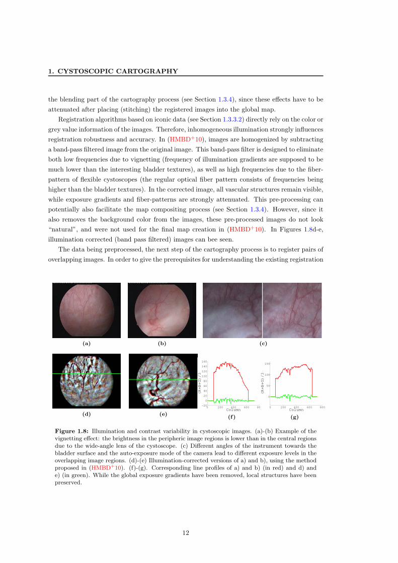
1. CYSTOSCOPIC CARTOGRAPHY
the blending part of the cartography process (see Section 1.3.4), since these effects have to be
attenuated after placing (stitching) the registered images into the global map.
Registration algorithms based on iconic data (see Section 1.3.3.2) directly rely on the color or
grey value information of the images. Therefore, inhomogeneous illumination strongly influences
registration robustness and accuracy. In (HMBD+10), images are homogenized by subtracting
a band-pass filtered image from the original image. This band-pass filter is designed to eliminate
both low frequencies due to vignetting (frequency of illumination gradients are supposed to be
much lower than the interesting bladder textures), as well as high frequencies due to the fiber-
pattern of flexible cystoscopes (the regular optical fiber pattern consists of frequencies being
higher than the bladder textures). In the corrected image, all vascular structures remain visible,
while exposure gradients and fiber-patterns are strongly attenuated. This pre-processing can
potentially also facilitate the map compositing process (see Section 1.3.4). However, since it
also removes the background color from the images, these pre-processed images do not look
“natural”, and were not used for the final map creation in (HMBD+10). In Figures 1.8d-e,
illumination corrected (band pass filtered) images can bee seen.
The data being preprocessed, the next step of the cartography process is to register pairs of
overlapping images. In order to give the prerequisites for understanding the existing registration
(a) (b) (c)
(d) (e)
0 200 400 600 800−20
0
20
40
60
80
100
120
140
160
Column
(R+
B+
G)/
3
(f)
0 200 400 600 800
0
50
100
150
Column
(R+
B+
G)/
3
(g)
Figure 1.8: Illumination and contrast variability in cystoscopic images. (a)-(b) Example of thevignetting effect: the brightness in the peripheric image regions is lower than in the central regionsdue to the wide-angle lens of the cystoscope. (c) Different angles of the instrument towards thebladder surface and the auto-exposure mode of the camera lead to different exposure levels in theoverlapping image regions. (d)-(e) Illumination-corrected versions of a) and b), using the methodproposed in (HMBD+10). (f)-(g). Corresponding line profiles of a) and b) (in red) and d) ande) (in green). While the global exposure gradients have been removed, local structures have beenpreserved.
12

1.3 2D Endoscopic Cartography
algorithms (explained in Section 1.3.3), 3D and 2D geometrical considerations are first provided
to the reader in Section 1.3.2.
1.3.2 Geometry of Cystoscopic Image Acquisition Systems
The displacement of the cystoscope between two image acquisitions has first to be mathemati-
cally defined to understand the geometrical link between the pixels of the images acquired from
two different viewpoints. For this reason, the instrument displacement is first shortly discussed
and the geometrical transformation parameters linking the images are then presented.
Three-dimensional Cystoscope Displacement
While the clinicians freely move the cystoscope inside the organ, the instrument’s displacement
between two acquisitions i and j corresponds exactly to a rigid 3D transformation
T3Di→j =
[R3D
i→j t3Di→j~0 1
]
. (1.3)
R3Di→j = RX(rX) RY (rY ) RZ(rZ ) is a 3D rotation matrix composed by 3 rotations with angles
rX , rY , rZ around the axes ~Xi, ~Yi and ~Zi of the camera of acquisition number i, centered at the
camera’s optical center Ci, with
RX(rX) =
1 0 00 cos(rX) − sin(rX)0 sin(rX) cos(rX)
; RY (rY ) =
cos(rY ) 0 sin(rY )0 1 0
− sin(rY ) 0 cos(rY )
;
RZ(rZ) =
cos(rZ) − sin(rZ) 0sin(rZ) cos(rZ) 0
0 0 1
.
t3Di→j = [tX tY tZ ]T
is a translation vector, where tX and tY are parallel to the image plane,
and tZ is orthogonal to the image plane.
Two-dimensional Image Geometry
As the cystoscope is moved closely to the bladder wall at a high acquisition rate, the geometry
of the bladder combined with the small FOV leads to the typical assumption made about
the 2D relationship between overlapping images. Indeed, since the bladder is filled with an
isotonic liquid and the time between two acquisitions is very short, the epithelial surface can be
considered as rigid (without movements and deformations) for small image sequences. Moreover,
in many regions of the filled bladder, the small FOV (the cystoscope is close to the epithelium)
visualizes quasi-planar surface parts. With such assumptions (which were confirmed by the
results of (BSGA09, HMBD+10, MLDB+08, BHDS+10)), the 2D geometrical link between
13

1. CYSTOSCOPIC CARTOGRAPHY
homologous pixels of two acquisitions i and j can be modelled as a homogeneous perspective
transformation (or homography). This transformation is defined as
T2Di→j =
Sx cosφ −sx sinφ txsy sinφ Sy cosφ ty
hx hy 1
, (1.4)
where (Sx, Sy) correspond to scale changes, (sx, sy) are shearing factors, and φ models the
in-plane rotation. Translations are given by (tx, ty), and (hx, hy) correspond to out-of-plane
rotations. Subscripts denote the x- and y-axes of the image plane.
A homogeneous position p2Di,k = [xi,k, yi,k, 1]T
of pixel k in the (source) image Ii is trans-
formed to its corresponding homogeneous sub-pixel position p2Dj,k′ = [xj,k′ , yj,k′ , 1]T in the (tar-
get) image Ij by
p2Dj,k′ = νk T2Di→jp
2Di,k , (1.5)
where νk is a normalizing factor, ensuring that the third element of p2Dj,k′ is equal to 1. The use
of indices k and k′ denotes homologous pixel positions, displaced from the coordinate system
of acquisition i into that of acquisition j. We will also use the terminology T2Di→j(Ii) to describe
the transformation (perspective warping) of an image Ii into the coordinate system of image
Ij . This transformation is computed using back-warping and bi-cubic interpolation.
Global perspective transformations (that transform pixel positions expressed in the local
coordinate system of acquisition i into a common global coordinate system) can be computed
via concatenation:
T2D0→i =
i−1∏
k=0
T2Dk→k+1. (1.6)
Equation (1.6) assumes (without loss of generality) that the coordinate system of the first
acquisition is used as the reference coordinate system.
Note that some contributions (BSGA09, BBS+10) use an affine version of Equation (1.4),
i.e. hx and hy are equal to zero and no perspective transformations are applied. While this has a
negligible visual effect for the registration of two subsequent images, concatenated global trans-
formations are changed noticeably due to accumulated errors, as the cystoscope displacement
is indeed fully perspective.
Cylindrical and Spherical Projections
It should be noted that for many cartography applications (i.e. consumer photography), it
is generally recommended to use cylindrical or spherical coordinates when constructing the
final panorama. This is due to the fact that the map tends to get deformed severely once the
FOV extends 90 degrees when using planar coordinates (Sze06). This effect is demonstrated in
Figure 1.9a. Using cylindrical or spherical coordinates, three-dimensional rotation of the camera
around its optical center simplifies the 2D geometry between images to translations and in-plane
rotations. As a consequence, images do not shrink/expand or get deformed perspectively, and
14

1.3 2D Endoscopic Cartography
(a) (b)
Figure 1.9: Planar vs. spherical coordinates. (a) Map created using the original images anda perspective projection model. The large FOV of the sequence leads to severe size differencesbetween the images. (b) Map created using spherical projection model. Camera panning reducesto translations of the projected images, leading to a panoramic image more pleasing to the eye.
the final panorama is more pleasing to the eye, as shown in Figure 1.9b. As the bladder
is (roughly) spherical, a spherical projection appears to be the ideal surface to project the
images onto. However, these models assume that the camera is only rotating around its own
optical center, and is not translated. This rules out using spherical coordinates for cystoscopic
cartography, as the instrument is mostly translated along the bladder wall. In practice, the
endoscope displacement does not correspond at all to a scenario where spherical coordinates
may be used.
Estimating T2Di→j
A homogeneous perspective transformation, as given by Equation (1.4), has eight degrees of
freedom. From Equation (1.5), we get two equations for each point correspondence:
xj,k′ (h31xi,k + h32yi,k + 1) = h11xi,k + h12yi,k + h13
yj,k′(h31xi,k + h32yi,k + 1) = h21xi,k + h22yi,k + h23,(1.7)
where hlm(l,m ∈ {1, 2, 3}) are the elements of T2Di→j (see Equation (1.4)). These equations are
linear with respect to the elements of T2Di→j , so that four point correspondences are sufficient
to determine T2Di→j up to scale. Using Equation (1.7), a homogeneous equation system to solve
for T2Di→j can be written:
A~h = ~0, (1.8)
with ~h containing the elements of T2Di→j . For exactly four point correspondences, A is an 8x9
matrix with rank 8 and has a one-dimensional Null-space that gives the exact solution for ~h.
When more than four point correspondences are available, Equation (1.8) is overdetermined
and has no exact solution, due to errors in the correspondences leading to a rank of A 6= 8.
Using the Singular Value Decomposition (SVD) technique (GR70), ~h can be approximated in
a least squares fashion.
In a similar way, the rigid 3D transformations T3Di→j can be estimated, which will be explained
in Chapter 4.
15
1. CYSTOSCOPIC CARTOGRAPHY
1.3.3 Registration of Cystoscopic Images
The geometry of the cystoscopic acquisition system being introduced, and the geometric model
used for superimposing overlapping images being defined, it is now possible to present exist-
ing contributions for the assessment of T2Di→j in the case of bladder images. The process of
superimposing the common area of partly overlapping images is called registration.
Feature Based Registration
Feature based approaches extract locations (key-points) in both images that are likely to be
discriminative, such as points located on corners or line segments. One of the early examples for
such a key-point extraction method is the Harris corner detector (HS88). For these key-points,
feature vectors are computed and can be used to measure the similarity between key-points
in different images. A variety of descriptors exist in the literature. Well known examples are
Scale Invariant Feature Transform (SIFT) (Low99) and Speeded Up Robust Features (SURF)
(BTVG06) features. These descriptors are scale and rotation invariant. More recently, Affine
Scale Invariant Robust Features (ASIFT) were proposed (MY09), which extend SIFT features
for affine transformation invariance. Other common feature descriptors are ORB (RRKB11), or
Histograms of Oriented Gradients (HoG) (DT05). Once key-points and descriptor vectors have
been computed for a pair of images, a search for corresponding key-points is performed. The
typical procedure is to find the best descriptor match for each key-point in the source image to
all descriptors of the target image’s key-points. From these initial matches, only those whose
score is by a certain factor better1 than the second best match are kept. Alternatively, another
initial outlier rejection is to also compute the best matches for all descriptors in the target
image, and only keep matches that agree in both directions (i.e. both from image Ii to image
Ij and vice versa). Since these initial matches still contain outliers, robust outlier rejection
methods, such as RANSAC (FB81) or LMedS (Rou84)), are performed to remove outliers and
fit the transformation.
This feature based image registration approach was used in (BSGA09, BBS+10) for images
acquired in the fluorescence modality. In (BSGA09), SIFT features are computed for a set of
key-points, while in (BBS+10), SURF features were used to decrease computation time in order
to work in a real-time framework. Both in (BSGA09) and in (BBS+10), RANSAC was applied
to estimate the affine transformation that registers consecutive images of cystoscopic video-
sequences. Images acquired in the fluorescence modality usually show strong vascular contrast,
so that image primitives (key-points in this case) can be robustly segmented and matched in
consecutive images throughout the sequence.
1In (Low99), a threshold of 0.8 is suggested.
16

1.3 2D Endoscopic Cartography
Feature Based Registration in the White Light Modality
In the more widespread (and standard) white light modality, less contrast is available, and
image primitives cannot be robustly extracted throughout the video-sequence systematically.
Figures 1.7a-c show cystoscopic images with contrasted vascular structures, which can robustly
be segmented and used for image registration. The remaining images do not contain enough
sufficient vascular structures (or they are only bundled in a small sub-region), and are (partly)
blurry due to de-focusing or the angle towards the bladder surface. When a well exposed
scan leads to well-contrasted images, registration using SURF features and RANSAC robust
fitting of a perspective transformation is feasible. Figure 1.10a shows the successful matching
of two consecutive images from a cystoscopic video-sequence. In the top row of each sub-figure,
the two input images that have to be registered are shown. In the middle row, green lines
depict reliable feature point correspondences, while red lines show rejected outliers. In the
bottom row, the first (source) image (left hand side) is warped onto the target image using the
estimated perspective transformation. Point correspondences are well spread in the overlapping
image regions, and consequently the superimposed source image is well aligned with the target
image. Figure 1.10b shows a pair of consecutive images from another cystoscopic sequence.
However, the images suffer from slight motion blur, and are less contrasted. These effects are
often caused by slow auto-exposure and auto-focus of the camera, or when the cystoscope is
further away from the bladder wall. The middle row of Figure 1.10b shows much more rejected
outliers, which indicates that feature correspondences are less unique when the images’ quality
decreases. While the estimated perspective transformation using inliers still leads to a visually
acceptable perspective warping of the source image, inliers are less well spread and are focused
on the vascular structure in the center of the images. Between two images the alignment errors
are usually not perceptible, but theses errors accumulate during the placement of the data in a
global map and often become visible in the map, as will be discussed latter.
Finally, Figure 1.10c shows a pair of non-consecutive images. While no previous contribution
to bladder cartography tries to register non-consecutive image pairs, they play an important role
in this thesis for global correction of the image placement in the common map coordinate system,
as will be shown later in Chapter 3. Only a few correspondences could be obtained after initial
outlier rejection, because the feature vectors are not invariant to perspective transformations or
strong appearance differences. Only 8 valid inliers were determined after RANSAC fitting, and
the superimposed images are incorrectly aligned. The results from Figure 1.10c demonstrate
that feature based registration cannot be robustly used for white light bladder cartography.
If only one pair of images is incorrectly superimposed, the final map will also be incorrectly
stitched.
17

1. CYSTOSCOPIC CARTOGRAPHY
(a) (b) (c)
Figure 1.10: Feature based registration in the white light modality. (a) Well contrasted con-secutive images without motion blur. Enough homologous SURF keypoints can be extracted andmatched with RANSAC. Green lines depict reliable feature point correspondences, red lines showrejected outliers. (b) Consecutive images, suffering from motion blur, de-focus and weak expo-sure. More rejected outliers and altogether less matches show that descriptors are less uniquewhen image quality decreases. The estimated perspective transformation still leads to an accept-able (visually coherent) superimposition of the images, but inliers are focused on the vascularstructures in the center of the images. (c) Registration of non-consecutive images, which differboth in contrast and exposure due to different angle and distance to the bladder surface. Only afew (mostly incorrect) correspondences could be obtained after initial outlier rejection. Such a lackof positive matches arises since feature vectors are not invariant to perspective transformationsand the strong appearance difference. Eight valid inliers were determined by RANSAC, but thesuperimposed images using the estimated transformation are incorrectly aligned.
Registration Based on Iconic Data
Two approaches based on iconic data were previously developed at the CRAN laboratory for
robustly registering bladder images in the white light modality. In (MLHMD+04, MLDB+08),
T2Di→j is obtained by maximizing the mutual information between the target image Ij and the
source image Ii transformed by T2Di→j(Ii). This work is based on EMpirical entropy Manipu-
lation and Analysis (EMMA), proposed in (VWI97). The mutual information is a statistical
measurement which combines the grey-level entropies E(Ij) and E(T2Di→j(Ii)) of the overlap-
ping parts of the images Ij and T2Di→j(Ii) and the joint grey-level entropy E(Ij ,T
2Di→j(Ii)). This
measurement can be written as
SMI(Ij ,T2Di→j(Ii)) = E(Ij) + E(T2D
i→j(Ii))− E(Ij ,T2Di→j(Ii))
and is maximized by a stochastic gradient descent algorithm, optimizing the transformation
parameters of T2Di→j . The grey-level entropies are computed using grey-level probability density
functions. Each probability density function is analytically modelled by the sum of about 300
18

1.3 2D Endoscopic Cartography
Gaussian functions with the same standard deviation. The value of the latter is optimized
together with the perspective matrix parameters. A large number of iterations is needed to
reach convergence, so consequently, this approach needs several hours to compute a panoramic
image from a video-sequence.
As discussed in detail in Section 1.5, the computation time is the least important aspect
(registration quality being the most important one), as maps are mainly used for a second diag-
nosis (after the actual examination) and bladder cancer follow-up. However, it is still desirable
to be able to make a the second diagnosis shortly after the examination. To achieve a fast
cartography algorithm, (HMBD+10) proposed to use a Baker-Matthews optical flow approach
that minimizes the sum of squared distances (SSD) of grey-values between overlapping images.
In order to increase the speed of convergence, they first compute an initial transformation using
cross-correlation in the Fourier domain, thereby obtaining an initial estimate of translation only
(parameters tx and ty in Equation (1.4)). The lack of strongly discriminative texture prevents
the computation of all transformation parameters of T2Di→j directly in the Fourier domain, oth-
erwise the method from (JJ06) might possibly be applied directly. Formally, the optical flow
approach of (HMBD+10) can be written as
SBM (Ij ,T2Di→j(Ii)) =
∑
p∈Ij∩T2Di→j
(Ii)
(Ij(p)− (T2Di→j(Ii))(p))
2
In (HSB+09), a study concerning robustness and accuracy of both optical flow and mutual
information based methods was conducted. For endoscope displacements consisting mainly
of translations, the two exiting methods register the images accurately. However, for T2Di→j
dominated by rotations, scale changes and/or perspective changes, both methods perform sig-
nificantly worse (the registration accuracy is up to ten times worse than for pure translations).
While this has only small visible effects on the registration of two subsequent images, the global
error accumulates drastically and is often visible in the maps. These results will be discussed in
more detail at the end of Chapter 2, where we compare the results of (HSB+09) with an initial
proof of concept for graph-cut based image registration, as published in (WDBH+na).
1.3.4 Map Compositing
The local T2Di→i+1 matrices registering consecutive images Ii and Ii+1 can be used to de-
termine the global matrices T2D0→i, as defined in Equation (1.6), which place each image Ii
in the map coordinate system (here that of image I0). Once theses global transformations
T2D0→i, i ∈ {0, ..., N − 1} have been estimated for all N images, the panoramic image can be
composed. This compositing process will also be referred to as stitching.
Often, this process is divided into several steps (Sze06). First, seams can be computed.
These seams determine the locations of transition between overlapping images in the global
map. This is equivalent to a labelled image, where each pixel p is assigned an image index
lp ∈ {0, ..., N − 1}, where lp means that image Ilp is used to obtain the color for pixel p in
19

1. CYSTOSCOPIC CARTOGRAPHY
the map. The position of these seams should be determined so that visible texture and color
discontinuities in the map are removed, or at least minimized. Such discontinuities can occur
due to small misalignments, or ghosting (moving objects in a static scene). Once these seams
are detected, blending methods try to correct exposure differences over seam borders. While
seam detection plays an important role in many stitching applications, hitherto, all previous
contributions to bladder cartography (MLHMD+04, MLDB+08, WRS+05, BBS+10, BGS+10,
BGS+11) omitted this seam detection step, even though such methods are of great interest
also for bladder cartography. The methods proposed in (BRM+09, MLHMD+04, MLDB+08)
directly compose the panoramic image by overwriting existing pixel values with those from
the current image. This leads to too dark maps when vignetting is strongly present, and to
visible exposure artefacts, as can be seen in Figure 1.11a. Other contributions perform blending
techniques to minimize composition artefacts at pixels in overlapping image regions.
Alpha-Blending
The most basic blending method is known as linear alpha-blending (PD84, Bli94). The pixels
p in the overlapping area IIi∩Ij between two images Ii and Ij (or the current panoramic image
and the next image to be stitched) are linearly interpolated using
IIi∩Ij (p) = αIi(p) + (1− α)Ij(p). (1.9)
This very simple linear interpolation method may work sufficiently when scene exposure vari-
ations are small. For cystoscopic images however, the vignetting-induced exposure differences
are still clearly visible after linear alpha-blending, as can be seen in Figure 1.11b, and also
introduces blurring across overlapping images.
Feathering
Slightly better results can be obtained by substituting the weighting parameter α of Equa-
tion (1.9) with a weighting function α(p), which weights pixels near the images’ center more
strongly than those in the peripheral regions (WRS+05). The weights can be computed using
any distance transformation (e.g the Euclidean distance transformation (ST94)), or the grass-
fire transformation (B+67). A similar method was proposed in (HMBD+10), where weights are
computed using the Gaussian function α(p) = 0.9e−r/(2σ) + 0.1, with σ equal to one quarter of
the image’s width, and r the distance of p to the image center. The result using a Euclidean
distance-weighted alpha-blending can be seen in Figure 1.11c. While artefacts due to vignetting
are mostly removed, a significant amount of blur is visible. Another possibility to chose the
weighting function is to use offline-calibrated endoscopic illumination characteristics, as pro-
posed in (BGS+10), which also reduces the vignetting-induced exposure loss at the peripheral
image regions.
20

1.3 2D Endoscopic Cartography
(a) (b)
(c) (d)
Figure 1.11: Examples of different map compositing techniques. The registration was performedusing the methods proposed in Chapter 3. (a) The map is iteratively overwritten with the currentimage, as applied in (BRM+09, MLHMD+04, MLDB+08). Artefacts due to the exposure differ-ences and vignetting are clearly visible at the images’ borders. (b) Alpha-blending (PD84, Bli94)with α = 0.75. Exposure artefacts are reduced compared to those in a), but still visible. Blurringartefacts are introduced. (c) Distance based alpha-blending (HMBD+10). Artefacts are mostlyremoved, but the degradation due to blur is stronger than in b). (d) Outlook and comparison tothe compositing techniques proposed in Chapter 3 of this thesis. No artefacts can be seen, andthe map’s contrast is greatly enhanced.
Multi-Scale Blending
Due to the freely moving cystoscope, individual images of a cystoscopic video-sequence often
show strong variations in map resolution (an image taken close to a lesion usually has a higher
panoramic resolution than an image captured from a larger distance when the clinicians try to
locate anatomical landmarks). Images also differ in exposure due to the distance and orientation
of the cystoscope with regard to the bladder surface. In the fluorescence modality, the rapidly
decaying fluorescence must also be taken into account when stitching the final panorama. If
images, acquired at a late stage of the examination, dominate the texture of the map, the
reddish glowing tumour tissue visible in earlier images will be lost. In order to obtain well
illuminated maps showing a maximum of fluorescence and resolution, a multi-scale blending
method was proposed in (BGS+10), and later extended to a non-linear multi-scale blending
method in (BGS+11). It is argued that well exposed images can only be acquired when the
cystoscope is moved at close distance to the bladder wall. For such acquisitions, bright images
correspond both to high fluorescence emission as well as to high resolution. The aim of the
21

1. CYSTOSCOPIC CARTOGRAPHY
multi-scale blending method is to exploit the images acquired close to the bladder wall to build
maps with high resolution and strong fluorescence signal.
This multi-scale non-linear blending method produces well exposed textured maps showing
fine vascular structures, as can be seen in (BGS+11). However, it does not consider the influence
of motion blur or de-focus, as images taken from similar viewpoints will have similar mean
brightness, independent of their contrast or sharpness. Furthermore, images taken from close
range are always preferred over images taken from further away, even if the former are blurry.
The image sequence shown in Figure 1.11 contains images taken all from approximately the
same distance to the bladder epithelium, so the multi-scale blending approach of (BGS+11) has
no apparent advantages over feathering methods in the white light modality.
1.3.5 First Assessment of Existing Endoscopic Cartography Approaches
As a first and brief evaluation of the published cartography approaches (see Section 1.5 for a
detailed discussion), it is possible to notice that the automatic registration of a large number
of images without a priori knowledge is an open problem in endoscopic applications in general,
and in cystoscopy in particular. Indeed, several steps of the existing endoscopic cartography
methods do not satisfy all conditions for automatic and visually coherent bladder map creation.
• The robust white light registration algorithms usually require large overlapping regions
between consecutive images (often at least 90% of the image area) and well contrasted
data (without blur). Feature-based approaches may not robustly estimate the geometric
relationship systematically, as sequences are often blurry or of weak contrast.
• There is no automatic detection of non-consecutive images with strong overlapping and
common regions (e.g. due to crossing endoscope trajectories). Such a detection is required
to correct the visual aspect of the maps.
• Blending algorithms minimizing the texture and color discontinuities are often not efficient
enough. Moreover, they also do not optimize the contrast of the maps, nor do they detect
optimal transitions (seams) between overlapping images.
1.4 3D Endoscopic Cartography
Two-dimensional cartography greatly facilitates diagnosis, preparation of follow-up examina-
tions, surgery planning and archiving of the recorded video in a single high resolution picture
(see Section 1.1). However, the organ is three-dimensional, and the mental orientation and rep-
resentation performed by the clinicians is intuitively done in 3D. In addition, three-dimensional
data presents valuable information during surgical interventions, especially for locating lesions
22

1.4 3D Endoscopic Cartography
with respect to anatomical landmarks or for roughly measuring the dimension of lesions. Con-
sequently, it can also be helpful to construct three-dimensional maps (or textured surfaces)
from the video-sequence acquired during a cystoscopic examination.
Unfortunately, as explained previously, the small FOV and the close distance of the cysto-
scope towards the bladder surface impedes the direct estimation of 3D data from the video-
sequence (using only the two-dimensional images, showing quasi-planar scenes). As shown in
the literature related to the few attempts of 3D analysis of endoscopic data, either a priori
information about the parametric surface of the organ, or additional 3D data is necessary to
robustly reconstruct the organ’s three-dimensional shape. In the following sections, we will
review the literature regarding the 3D reconstruction of endoscopic medical data.
1.4.1 2D Endoscopic Cartography with 3D a priori Knowledge
When the observed scene can be represented as a parametric surface of known shape, the images
can be registered using the known surface geometry as an a priori information. This reduces
distortions due to the projection of the three-dimensional scene onto the image plane. In
(CS09), this approach was used to construct maps of the inner oesophagus wall using tubular
3D shapes. The method computes both the endoscope trajectory T 3D and a 2D panoramic
image. Although not done in (CS09), the registered images could be projected onto the tubular
shapes to obtain a 3D representation of parts of the inner oesophagus wall.
More specific for bladder cartography, the method of (BSGA09) represents the bladder
surface using “hemicube” planes. Each hemicube plane approximates a part of the bladder’s
surface (back wall, left and right lateral wall, upper wall and ostium) as a plane. For each
of these regions, a seperate scan is performed by the clinician, and the computed 2D map
is associated with this hemicube. The justification for this procedure is to prevent severe
perspective distortions arising when projecting the entire spherical bladder surface on a single
planar map (see also Figure 1.9). Using seperate hemicubes, distortions remain low, and the
entire bladder map can be displayed by unfolding all hemicube planes. The main disadvantage
is the fact that the clinicians must manually select the corresponding hemicubes while scanning
the bladder, and must scan each hemicube separately. This may impede the clinicians’ own
standard procedure of scanning the organ’s surface, and does not guarantee seamless transitions
from one hemicube to the other. Additionally, the map is constructed only up to scale and does
not allow for the measurement of dimensions in world coordinates. Nonetheless, it depicts an
interesting approach of a semi-3D cartography approach, which can be easily archived in a
single high resolution (unfolded) image.
23
1. CYSTOSCOPIC CARTOGRAPHY
1.4.2 3D Endoscopic Cartography
In a calibrated stereo (or multi-camera) setup (i.e. with known intrinsic and extrinsic param-
eters), 3D points can be reconstructed if their homologous 2D pixel positions can be detected
and matched between two or more viewpoints. However, as the instrument is moved freely, its
trajectory (i.e. the extrinsic parameters, encapsulated in T3Di→j) is unknown. Structure from
motion (SfM,(PKG99, HZ03)) approaches, which are based on bundle adjustment (TMHF00),
tackle this problem by simultaneously estimating 3D points and camera displacement from sev-
eral viewpoints. This approach was used to estimate the surface of the bladder in (SPS12).
As a first step, images are registered using SIFT and RANSAC, and the 2D map is globally
corrected to obtain more accurate transformation between consecutive and non-consecutive im-
ages. While this is theoretically possible using iconic data registration, it implies very long
computation times and a robust automatic detection of non-overlapping images (which is still
an open problem). In (SPS12), an initial 3D point reconstruction is then computed with the
constraint that the 3D points must lie on a sphere (a geometric constraint that is not fulfilled in
practice). Finally, an incremental bundle adjustment step iteratively moves the reconstructed
points towards the true surface shape. The final 3D map is obtained by fitting a surface on the
reconstructed points, and projecting the 2D images onto it.
The algorithm was tested on a pig bladder phantom injected with contrast dye. This dye
strongly increases the contrast of vascular structures and ensures the presence of image prim-
itives which can be easily segmented. As was argued before, image primitive extraction can-
not be systematically guaranteed with human bladder tissue in realistic (clinical) conditions.
Nonetheless, the estimated perspective transformations T2Di→j could be used to create artificial
correspondences for the bundle adjustment step. However, a main restriction is the fact that
the cystoscope must be close to perpendicular at all times during the acquisition to ensure
the convergence of the method. More specific, in (SPS12), a specifically designed instrument
(an ultra-thin optical fiber) was placed near the center of the phantom, and was automati-
cally rotated by a robotic system around its origin to scan the entire phantom from the same
viewpoint. This ensures both perpendicular orientation to the bladder wall, as well as enough
three-dimensional structure (non-planar) in each image. These assumptions do not hold with
rigid endoscopes for practical reasons (the clinician cannot manoeuvre a rigid cystoscope to be
in such a situation). Even with fiber-scopes, this is a challenging task for clinicians and would
require intensive training. In addition (for both rigid and flexible cystoscopes), the instrument
must be displaced much closer to the bladder surface in order have sufficient brightness and
texture resolution in the images, which loses valuable three-dimensional structure (FOV shows
quasi-planar structures). Furthermore, bundle adjustment is sensitive to the initial solution,
and the bladder is often not spherical, as other organs warp it. Moreover, this approach requires
the entire bladder to be scanned and globally registered, which is a challenging (and still open)
problem with clinical cystoscopic data.
24

1.4 3D Endoscopic Cartography
1.4.3 3D Endoscopes
The methods presented in the previous section only use 2D images to recover the organ sur-
faces. Alternatively, endoscopes that also provide 3D information could allow for a more robust
estimation of the surface geometry. Most solutions described in the literature are based on the
active stereo-vision principle. In comparison to passive stereo-vision, the use of a light projector
facilitates the matching and reconstructions steps in the case of complex medical scenes. For
two channel endoscopes, there is a direct way to implement the active stereo-vision principle.
One channel projects light patterns (such as lines, scattered points, or structured light patterns)
onto the surface, while the other channel acquires the projected patterns. When both projector
and camera are calibrated, the projected pattern can be used to determine 3D positions in
the camera coordinate system. In (CLZQ03), it was shown that for a relatively small baseline
(distance between projector and camera channel axes) of 2 mm, points on test objects can
be reconstructed with sub-millimeter accuracy. This system was also used to reconstruct the
surface of the oral cavity. In (ADG09), the authors have used the same principle to reconstruct
the abdominal cavity using a coded pattern that facilitates the matching between the pattern
and its projection. While these two approaches lead to very robust estimation of dense surfaces
for small FOV endoscopes, the projected patterns suppress the color information of the organ
and are not suitable for cystoscopic cartography. In addition, the almost planar surface seen in
each FOV in a cystoscopic setup impedes a robust registration. For instance, if the cystoscope
is displaced along the bladder wall, while its distance and (out-of-plane) orientation towards
it remains constant for two acquisitions, the same planar surface will be recovered. In such a
scenario, the endoscope displacement is ambiguous and cannot be recovered robustly.
This ambiguity can be overcome by guiding the 3D registration using 2D textures. At the
CRAN laboratory, an active stereo-vision prototype (whose implementation on a one-channel
endoscope is currently in progress) for two-channel endoscopes was proposed using an eight
laser dot structured light pattern (BHDS+10). After projector-camera calibration (BHSD+10),
3D positions of these eight laser dots in the camera coordinate system are acquired in addition
to each color image. The rigid 3D cystoscope displacement T3Di→j , given in Equation (1.3), is
estimated together with the corresponding T2Di→j perspective transformation registering consec-
utive image pairs. As detailed in (BHDS+10), the inner 3D bladder surface construction is
guided by the registration of 2D images. This algorithm exploits some constraints relating to
the 3D and 2D prototype geometry and the 3D/2D laser point correspondences to ensure a
robust 3D surface construction. After the surface has been built, the 2D image textures can be
projected onto it.
Recently, in (PHS+09), a 3D endoscope was built with a time-of-flight (ToF, (LSKK10))
camera. Each pixel of a ToF camera provides a distance from the surface. This system was used
to reconstruct surfaces of the inner wall of a pig stomach using a laparascope. The modulated
infrared light was emitted through an optical fiber, and the distance images were acquired
25

1. CYSTOSCOPIC CARTOGRAPHY
through the endoscope channel. Similar to the dense active stereo-vision systems described
in the first paragraph, using almost planar surfaces in each FOV, the ambiguity (due to poor
geometrical information) impedes a robust estimation of the endoscope displacement since the
3D shapes cannot be registered without additional texture information.
However, as described in Chapter 4, the ToF based surface measurement principle can be
implemented on one-channel endoscopes (such as cystoscopes equipped with color cameras)
using commercially available beam splitters. This would allow to simultaneously acquire the
distance images from the ToF camera and the color images of a CCD camera. After offline
stereo calibration of both cameras, these distances can be transformed into 3D positions in the
color camera coordinate system. Such a system could therefore supply a high resolution color
image and a low resolution 3D point cloud. 2D image registration algorithms can then be used
to guide either 3D-3D data superimposition algorithms or to solve 2D-3D point correspondence
problems with the aim to find the T3Di→j rigid transformation (see Equation (1.3)) linking two
endoscope positions.
1.4.4 First Assessment of Existing 3D Endoscopic Cartography Approaches
The literature (SPS12) shows that the complexity and inherent variability of endoscopic data
complicates a robust construction of 3D bladder maps. However, the publications of active
stereo-systems (CLZQ03, ADG09) dedicated to endoscopy have shown that this measuring
principle can be a solution to recover 3D organ information in a robust way. Moreover, it was
shown in (BHDS+10) that 3D cartography of textured large FOV data is possible and can be
guided by 2D image registration.
1.5 Objectives of the thesis
The main and general aim of this thesis is to robustly build 2D large FOV textured maps from
the images of a cystoscope acquired for unknown and realistic (crossing) trajectories, which
were not handled in previous contributions. The existing algorithms lead to visually incoherent
panoramic images for such instrument displacements. A second goal of this thesis is to show the
feasibility of 3D cystoscopic cartography. To do so, the 2D algorithms have to be adaptable to
3D cartography. To meet these objectives, different and challenging problems have to be solved.
The following sections summarize the scientific and medical objectives of this dissertation.
1.5.1 Scientific Objectives
The main scientific objectives (in bold) addressed in Chapters 3 and 4 are formulated as follows.
26

1.5 Objectives of the thesis
Globally Coherent Transformations
No previous contribution automatically handles the case of partly overlapping, non-consecutive
image pairs. However, as the examination progresses, clinicians regularly return to previously
visited locations on the bladder surface (e.g. to regularly locate the cystoscope with respect
to an anatomical landmark, or to scan the epithelium in a systematic way). Possible instru-
ment trajectories are zig-zag-paths (the cystoscope performs multiple overlapping line-scans),
or loop-scenarios. In these cases, small local registration errors accumulate to larger global
cartography errors, leading to visible misalignments in the map when returning to previously
scanned areas. Without global correction of the local and global transformation matrices, the
final map will be incoherently stitched. Global correction thus requires registration of additional
(non-consecutive) image pairs.
The authors of (MLDB+08) have proposed a method to correct such misalignments, by
equally distributing the global errors between first and last image in loop scenarios using steepest
gradient optimization. However, no means of automatically detecting these loops is given, and
their algorithm is unable to register pairs of images with less than 90% of overlap, which is
seldom the case in such scenarios.
In (BTGA11), a system to detect gaps (e.g. missed parts in zig-zag- and loop-scenarios) was
proposed. Using this information, clinicians could potentially be able to re-scan these unseen
regions to fill holes in the panoramic image. However, only phantom image sequences were used
in (BTGA11), which significantly reduces global errors. Consequently, the authors did not deal
with correction of global errors. Clinical studies are currently conducted by the authors of
(BTGA11), and probably global errors will be an issue there.
One aim of this thesis is the design of an automatic overlap detection algorithm. For this
purpose, overlapping non-consecutive image pairs must be detected and registered accurately.
Accumulated errors have to be distributed equally over all possible image pairs, so that globally
coherent panoramic maps can be composed. The corresponding contributions are presented in
Section 3.2.
Robust and Accurate Image Registration
As stated in Sections 1.3 and 1.3.3, the intra- and inter-patient texture variability, as well as
motion blur and camera de-focus, involve several challenges to image registration algorithms
(see again Figure 1.7). Feature based image registration methods (BSGA09, BBS+10) on the
one hand are able to estimate the transformations that superimpose partly overlapping images
in an accurate fashion. However, such an approach is only feasible when the images are well
focused and do not exhibit strong perspective, focus, or exposure differences. This directly rules
out the registration of non-consecutive images (see previous section), because these effects are
almost always present due to the freely moving cystoscope (causing strong perspective changes)
and the auto-focus and auto-exposure mode of the camera attached to the instrument. It also
impedes the registration of images taken while the cystoscope is displaced rapidly, as the motion
27

1. CYSTOSCOPIC CARTOGRAPHY
blur removes valuable vascular structures and prevents the extraction of enough homologous
key-points.
Approaches based on iconic data on the other hand (MLDB+08, HMBD+10) do not rely on
the segmentation of image primitives and work more robustly in the mentioned scenarios, but
their accuracy suffers when rotations, scale and/or perspective changes become more dominant
(HSB+09). While consecutive image pairs are often related mainly by translations, the other
parameters are dominant when the endoscope changes its direction, and especially on non-
consecutive image pairs. Furthermore, these methods usually need a large percentage of overlap
(90% or more). While this is a reasonable assumption for consecutive image pairs, the overlap
percentage is often much less than 65% between non-consecutive images.
For these reasons, another objective of this thesis is to design and implement a registration
algorithm that works equally robustly and accurately, independent of the transformations in-
volved. It must be able to register non-consecutive image pairs with a low amount of overlap, so
that global map correction (see previous section) can be achieved. This objective is addressed
in Section 3.3.
Map Compositing
As was stated in Section 1.3.4, all previous contribution omit the step of detecting optimal seam
lines for the composition of the final panoramic image. Instead, overlapping images are directly
blended into a global textured map. While some of these methods are able to produce maps
without visually visible artefacts (and enhance the map in the fluorescence modality based on
the images’ intensities), blending-induced blurring and ghosting are the direct consequences of
the previously proposed methods.
Another aim is therefore to superimpose overlapping images while maximizing the contrast
of the textured maps. Seam lines must be selected so that no visible artefacts due to misaligned
vascular structures are present, images with good focus are preferred over blurry ones, and the
final map must not show any exposure related artefacts. This objective is met in Section 3.4.
Extendibility to 3D Cystoscopic Cartography
The main focus of this thesis is 2D cystoscopic cartography, because clinical data providing
additional 3D measurements (see Section 1.4) are not available yet. However, it is another aim
of the thesis to develop and implement the algorithms in a way that they can be extended to
work on 3D data. The algorithms must be modular in a sense that only the formulas explicitly
based on 2D data need to be re-implemented for 3D, while remaining steps and the global
algorithmic approach should not need modifications. Initial tests on phantom data (simulated
and acquired in the laboratory) should show the potential for clinical applications in the future.
These extensions to three-dimensional cartography are addressed in Chapter 4.
28

1.5 Objectives of the thesis
1.5.2 Medical Interest and Time Constraints
Although real-time cartography algorithms could be of interest for online wide FOV visualiza-
tion (e.g. to show clinicians whether they have missed/overseen some parts of the bladder wall),
building a map offline (i.e. the methods proposed in this thesis cannot be used in a real-time
application) can also lead to real medical progress. The following reasons strengthen this point.
• Recording a large FOV map is an efficient way to archive important examination infor-
mation. It is recalled that currently only a bladder sketch and a small FOV picture are
archived. Videos are not recorded since they are usually not exploitable by clinicians
who did not perform the examination. Even the clinicians who did it lose the ability to
understand the video after some time has passed. A wide FOV panoramic image, both
including the whole lesion and anatomical landmarks, allows for scene understanding (e.g.
lesion type, lesion localisation in the bladder, lesion state) for all clinicians. This fact en-
sures the traceability of examinations and surgical treatments over time for a disease that
usually requires a long time follow-up. This aspect of the work rather demands accurate
and robust cartography algorithms than fast ones.
• The other interest of large FOV bladder maps lies in the fact that other clinicians than the
urologist or surgeon who performed the examination can pose a second or third diagnosis.
Again, the confronting of several diagnoses does not require real-time cartography.
• As mentioned, to facilitate a diagnosis, the maps should be built in a robust and precise
way, rather than at image acquisition rate. However, computation times not exceeding a
quarter or a half hour enable clinicians to pose a second diagnosis, without requiring the
patient to stay for a long time at the hospital. The clinician/patient discussion (interview)
can then take place after the second diagnosis.
• Comparing visually (or automatically) two maps built with data acquired in intervals
of some weeks or months potentially facilitates lesion evolution assessment. Such an
assessment also does not require real-time cartography.
1.5.3 Global Approach: Discrete Energy Minimization as a Framework forCystoscopic Cartography Algorithms
As described in detail in Chapter 2, the use of graph-cuts to solve discrete energy minimization
problems has shown great potential in many applications of image processing and computer
vision. Such techniques have been successfully applied in various areas (segmentation, pre-
processing, disparity estimation, object detection, and many more) due to the flexibility they
allow in formulating tailored energy functions. Results are generally of high quality, which made
graph-cuts a popular field of research since the late 90s. We believe these techniques can be used
29

1. CYSTOSCOPIC CARTOGRAPHY
for many steps of the cystoscopic cartography process, and can outperform many of the existing
approaches. The final (but not least important) goal of the thesis is therefore to demonstrate the
potential of discrete energy minimization models for difficult image registration problems and
for producing high quality panoramic images and textured surfaces. While these algorithms
can hardly be implemented at acquisition rate, they should fulfil the third constraint of the
previous paragraph, so that the clinician/patient interview after the examination can benefit
from a large FOV textured map.
30

Chapter 2
Graph-Cut Optimization
This chapter presents an overview of discrete energy minimization using graph-cuts, and aims
at providing a self contained introduction to the topic. Basic notations used throughout this
dissertation will be introduced.
2.1 Discrete Energy Minimization in Computer Vision
Many problems that arise in image processing and computer vision, such as image segmentation
(BJ01, BFL06, BRB+04, RKB04), de-noising (BVZ01, Ish09), disparity estimation (BVZ98,
KZ01, BVZ01, KZ02, WAB03, LRR08, GHN+10), or photomontage and stitching (KSE+03a,
ADA+04, LI07), can be solved using discrete energy minimization techniques. A typical form
for such an energy function to be minimized is given in Equation (2.1):
E(x) =∑
p∈V
Ep(xp) +∑
(p,q)∈N
Epq(xp, xq), (2.1)
where x : V→ L is a configuration (or labeling) that maps every p ∈ V to an element x(p) from
a set of labels L, and N ⊆ V × V is a neighborhood system defined on the set V. To enhance
readability, we define xp := x(p). Often, an image I : V → Rm maps the set of pixels V ⊂ Z
2
defined on a finite grid to Rm (e.g. m = 1 for gray-scale, m = 3 for RGB color images), and N
denotes a neighborhood system defined on this grid. The configuration x then corresponds to
a certain assignment of labels (e.g. grey-values) to each pixel. In discrete optimization, the set
of labels L is finite, as opposed to continuous optimization, where L ⊆ R. While algorithms
may internally represent L as a set of (linearly ordered) integer values, each discrete label may
map to a real value, or may be associated with a symbolic meaning. For example, in disparity
estimation, the labels are displacement vectors in Rn, while for binary segmentation, the set of
labels is L = {“background”, “foreground”}.
31

2. GRAPH-CUT OPTIMIZATION
2.1.1 Order and Interaction
In Equation (2.1), Ep is often referred to as a unary term, while Epq is known as a pairwise term,
due to the number of dependent variables. We say a function E(x) is of order k when it consists
of terms with at most k + 1 interdependent variables. Following this definition, Equation (2.1)
is of order 1, or a first-order energy function, since it involves at most two dependent variables
p and q. In general, a kth-order energy function
E(x) =∑
c∈C
Ec(xc) (2.2)
consists of a set of cliques C1 whose number of variables in each clique c is at most k+1, where
xc = {xp | ∀p ∈ c} encodes the configuration of the variables in the clique. Equation (2.1)
consists of cliques of size 1 (e.g. the unary terms) and of size 2 (e.g. the pairwise terms).
The functions Ec(xc) are also called potential functions. Direct neighbours of a variable p are
defined in the set Np.
In practice, Ep(xp) often measures a similarity to observed data (i.e. how likely pixel p is to
be labeled xp). Therefore it is often referred to as the data term. With Epq(xp, xq), one usually
models spatial coherence, such as piece-wise smooth disparity fields. Consequently, it is often
called interaction or smoothness term. However, data terms may also be expressed using first-
or higher-order potential functions, as will be seen in Chapters 3 and 4.
2.1.2 Markov Random Fields
Energy functions, such as those in Equations (2.1) and (2.2), are closely related to probability
distributions of Markov Random Fields (Li95). A random field X = [X1, ..., Xp, ...XN ] consists
of N random variables, and X = x is the before mentioned configuration, where every variable
may be assigned a value xp ∈ L. All possible configurations, given a label set L, are defined
as the set X. Each assignment can be associated with a probability Pr(Xp = xp), or in short
Pr(xp). The joint probability for a configuration of the entire random field is then defined as
Pr(X = x) = Pr(x). If X is a Markov Random Field, it satisfies the following properties (for a
given N):
Pr(x) > 0, ∀x ∈ X (Positivity property)Pr(xp| {xq : q ∈ Np}) = Pr(xp| {xq : q ∈ V \ {p}}) (Markovian property)
Then, according to the Hammersley-Clifford theorem (HC71, Bes74), the joint probability dis-
tribution can be written as a Gibbs distribution:
Pr(x) =1
Ye−
∑c∈C
Ec(xc) with Y =∑
x∈X
e−∑
c∈CEc(xc)
1 In graph theory, a clique in an (undirected) graph G = (V, E) is a subset of the set of vertices C ⊆ V, sothat every pair of vertices in C is connected by an edge e ∈ E. Here, the term clique will be used also informallyto group the number of interdependent variables of an energy function.
32

2.2 Energy Minimization using Graph-Cuts
where Y is known as the partition function. The corresponding Gibbs energy can be obtained
from the negative logarithm of its distribution:
EGibbs(x) = − log (Pr(x)) = − log
(1
Y
)
+∑
c∈C
Ec(xc) = const + E(x).
Therefore, the maximum a posteriori solution (i.e. the most probable labeling) x∗ of X, given
by
x∗ = arg maxx∈LN
Pr(x),
can be found by minimizing E(x).
2.2 Energy Minimization using Graph-Cuts
MRFs as a framework for modelling energy functions such as those of Equation (2.1) have been
known to the computer vision community since the seminal work presented in (GG84) in the
mid-eighties. At that time however, a lack of efficient optimization techniques impeded a broad
use. Deterministic algorithms, such as iterated conditional modes (Bes86) or highest confidence
first (CB90), often only converge to poor local minima. A stochastic method like simulated
annealing (KGJV83) is theoretically able to obtain the minimum cost solution, but in practice,
the temperature decrease process demands great attention to be paid to the algorithm’s param-
eters, which impedes practical use on large datasets. Other used methods include max-product
loopy belief propagation (Pea88) and tree-reweighted message passing (WJW02).
In the late nineties, the use of max-flow/min-cut algorithms (FF56, FF62) to solve pairwise
MRFs revived the interest of energy minimization for many computer vision problems. They
have been shown to outperform other related methods in both quality and speed (see also
(SZS+08) for a thorough comparative study of different energy minimization techniques on
a set of representative benchmarks). Most of the algorithms developed in this dissertation
use this graph-cut framework to minimize energy functions designed for solving the objectives
formulated in Chapter 1. Therefore, the following sections are devoted to the introduction of
basic formulations. It will be shown how energy functions like that of Equations (2.1) and (2.2)
can be expressed in a graph-cut framework and minimized efficiently.
2.2.1 The st-Mincut/ Maxflow Theorem
General Definitions
In graph theory, a network flow can be used to model systems in which resources travel from one
location to another (Cor01). Examples are traffic along roads, fluids in pipes, or data sent over a
33
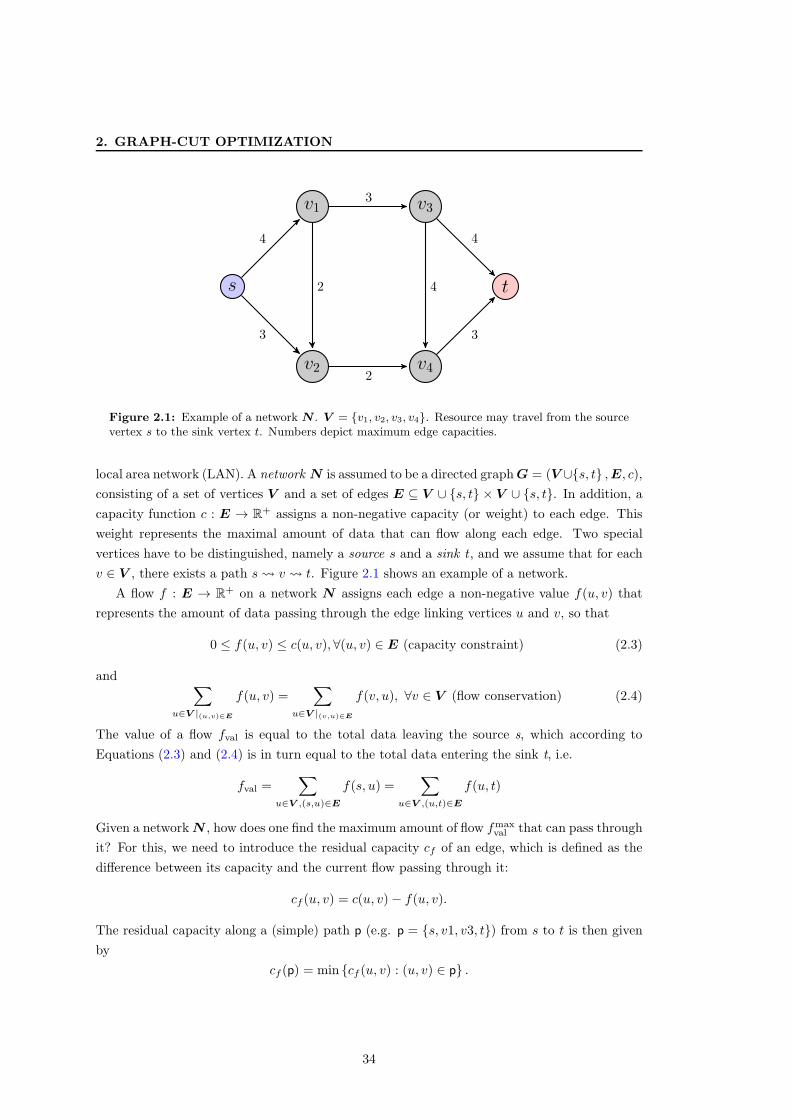
2. GRAPH-CUT OPTIMIZATION
s
v1
v2
v3
v4
t
4
3
3
2
2
4
3
4
Figure 2.1: Example of a network N . V = {v1, v2, v3, v4}. Resource may travel from the sourcevertex s to the sink vertex t. Numbers depict maximum edge capacities.
local area network (LAN). A network N is assumed to be a directed graphG = (V ∪{s, t} ,E, c),
consisting of a set of vertices V and a set of edges E ⊆ V ∪ {s, t} × V ∪ {s, t}. In addition, a
capacity function c : E → R+ assigns a non-negative capacity (or weight) to each edge. This
weight represents the maximal amount of data that can flow along each edge. Two special
vertices have to be distinguished, namely a source s and a sink t, and we assume that for each
v ∈ V , there exists a path s v t. Figure 2.1 shows an example of a network.
A flow f : E → R+ on a network N assigns each edge a non-negative value f(u, v) that
represents the amount of data passing through the edge linking vertices u and v, so that
0 ≤ f(u, v) ≤ c(u, v), ∀(u, v) ∈ E (capacity constraint) (2.3)
and∑
u∈V |(u,v)∈E
f(u, v) =∑
u∈V |(v,u)∈E
f(v, u), ∀v ∈ V (flow conservation) (2.4)
The value of a flow fval is equal to the total data leaving the source s, which according to
Equations (2.3) and (2.4) is in turn equal to the total data entering the sink t, i.e.
fval =∑
u∈V ,(s,u)∈E
f(s, u) =∑
u∈V ,(u,t)∈E
f(u, t)
Given a networkN , how does one find the maximum amount of flow fmaxval that can pass through
it? For this, we need to introduce the residual capacity cf of an edge, which is defined as the
difference between its capacity and the current flow passing through it:
cf (u, v) = c(u, v)− f(u, v).
The residual capacity along a (simple) path p (e.g. p = {s, v1, v3, t}) from s to t is then given
by
cf (p) = min {cf (u, v) : (u, v) ∈ p} .
34

2.2 Energy Minimization using Graph-Cuts
s
v1
v2
v3
v4
t
3|4
2|3
3|3
0|2
2|2
0|4
2|3
3|4
Figure 2.2: Maximum flow of the network shown in Figure 2.1. Edge numbering depictf(u, v)|c(u, v). The bottleneck (red edge numbers) is equivalent to the minimum cut, separat-ing the vertices into S (blue) and T (red). The flow along edges linking the source set with thesink set is equivalent to the amount of flow leaving the source / entering the sink, and equivalentto the maximum flow of the network. Note that the distribution of flow (unlike the maximumflow) is not unique, other valid flows with equal min-cut/max-flow are possible.
If cf (p) is strictly positive (cf (p) > 0), then p is called an augmenting path, and cf (p) more
data could flow along p without voiding Equations (2.3) and (2.4). Consequently, if there exists
an augmenting path in N , the flow is not maximal. A cut C of N , formally
C = (S,T ),S ∪ T = V ∪ {s, t} , s ∈ S, t ∈ T
is a partition of the vertices into two disjoint subsets S and T , where S is called the source set,
and T is called the sink set. The capacity (or cost) of such a cut Cval is the sum of capacities
of all edges (u, v) from the source set that are part of the cut:
Cval =∑
u∈S,v∈T ,(u,v)∈E
c(u, v).
The cut, for which the capacity is minimal, is called the minimum cut (or st-min-cut). It is
intuitive to see in Figure 2.2 that this cut represents the global bottle-neck of the network N ,
and that its capacity Cminval is equal to the maximum flow fmax
val passing through the network.
The next sections will introduce algorithms for solving the st-mincut/maxflow problem.
Mincut/Maxflow Algorithms
Augmenting Path Algorithms
The basic augmenting-path algorithm (FF56, FF62) iteratively pushes flow along augmenting
paths until the maximum flow is reached. Initially, there is no flow going from the source to the
sink, e.g. fval = 0. In each iteration, the algorithm finds an augmenting path p and pushes cf (p)
35

2. GRAPH-CUT OPTIMIZATION
more flow through it, thereby saturating it and removing it from the list of augmenting paths.
In the original Ford-Fulkerson version (FF56, FF62), augmenting paths are searched using a
depth-first strategy. This implies that each path of the graph is explored as far as possible
before backtracking. The maximum flow is reached when no augmenting path can be found,
which means each path p crosses as least one saturated edge. These saturated edges represent
the minimum cut boundary. When edge capacities are integers, the algorithm complexity is
bounded by O(|E| fmaxval ) because each augmenting path can be found in at maximum O(|E|)
time using depth-first search, and the flow is increased by at least 1 for each augmenting path.
For irrational flow values, convergence is not guaranteed (not even convergence towards the
maximum flow) (Zwi95).
Improved versions, independently published in (Din70) and (EK72), find shortest paths
using a breadth-first search (as opposed to depth-first search in (FF56, FF62)). These methods
are guaranteed to converge independently of fmaxval . First, all shortest paths of a fixed length
l1 are found and augmented. Then, a new breadth-first search for paths of length l + 1 using
the remaining unsaturated edges are searched from scratch. In this way, theoretical complexity
is strongly diminished. Indeed, the worst case complexity of (Din70) is O(|E| |V |2), and
O(|E|2 |V |) for (EK72).
Push-Relabel Algorithms
A different approach is used in push-relabel algorithms. These do not maintain a valid flow
throughout the computation, since active vertices may have a positive flow excess. Excess flow
is then pushed towards active vertices with a smaller distance to the sink. Un-pushable flows
are eventually pushed back to the source. The general push-relabel algorithm has a complexity
of (O(|V |2|E|). An implementation of (GT88) has a complexity of O(|V |3) when using a queue
(FIFO) based vertex selection rule, and O(|V |2√
|E|) when using a highest active vertex based
selection rule.
Boykov-Kolmogorov Algorithm
In practice, the max-flow algorithm proposed by Boykov and Kolmogorov in (BK04) is the most
efficient version when applied to dense 2D or 3D graph structures, which are commonly used
in computer vision problems. It can be seen as a heuristic variation of the augmenting-path
algorithms (FF62, Din70, EK72). Indeed, the difference is that in (BK04), new paths from the
source to the sink are not searched from scratch in each iteration, but previously found paths
are stored in a search tree structure. This structure contains two search trees, a source tree and
a sink tree. These trees contain the vertices associated with each terminal (“labeled vertices”).
Vertices not associated with a search tree are called “unlabeled”. In addition, a flag for each
vertex stores its state (active or passive). Initially, only the source and the sink are labeled and
marked as active (i.e. all other vertices are initially unlabeled and marked as passive). The
1For the breadth-first search, unit length edges are used. The shortest path of length l is therefore a pathfrom s to t that spans l edges.
36

2.2 Energy Minimization using Graph-Cuts
algorithm then iteratively performs the three stages refered to as “growing stage”, “augmenting
stage” and “adopting stage”. These stages are described in the next paragraphs.
Growing stage. Active vertices add passive and unlabeled neighboring vertices to their
search tree if their connecting edge has a residual capacity greater than zero. These newly
acquired vertices in turn become active. Once all neighboring vertices and their edges to the
current vertex have been evaluated, the current vertex is marked as passive (but retains its
label). This step is repeated with the remaining active vertices of the trees until either no more
active vertices remain, in which case the algorithm terminates and the st-mincut is found. Or
until an active vertex finds an unsaturated edge to a vertex from the other search tree, which
means a that an augmenting path p from the source to the sink is found.
Augmenting stage. If an augmenting path p was found in the previous stage, it is augmented
by increasing the flow by cf (p) along all of its edges, similar as in (FF62). In this stage however,
the search trees may transform into forests (i.e. a vertex can become the root of a new tree). A
new tree maybe be generated, since at least one saturated edge is created during the augmenting
step. If such a saturated edge lies between a vertex and its associated vertex terminal, the former
cannot be reached from the the terminal vertex, according to the search tree criteria allowing
only unsaturated edges.
Adopting stage. In this stage, the search trees are rebuilt. For each orphan (a labeled
vertex that can be reached from its associated terminal only through saturated edges after the
augmenting stage), new parents are searched. If through an edge to a neighboring vertex, an
unsaturated path to the same terminal can be found, this vertex becomes the new parent in
the search tree. If no parent can be found, the vertex is marked as unlabeled, and its children
are marked as orphans. These steps are repeated until no orphans are left.
An illustration of the different steps of the Boykov-Kolmogorov maxflow algorithm is shown
in Figure 2.3. In the initial stage (Figure 2.3a), only s and t are active (blue and red indicates
active vertices of the source/sink trees. Light blue and red vertices are passive vertices of their
tree, white vertices are unlabeled. Red edges are saturated and cannot be used in search trees).
In the following growing stage (starting with the source tree, see Figure 2.3b), s finds in p and
q passive, unlabeled vertices, and adds them to its search tree. Then s becomes passive. The
next step is the growing stage from the sink tree (Figure 2.3c). t finds in p a vertex from the
opposite search tree. This starts the augmenting stage, where the path {s, p, t} is augmented
by the bottleneck residual capacity 1. In the following adoption stage, no orphan vertex is
found, as p is still connected to its terminal through an unsaturated edge. Then the growing
stage of the sink tree is continued (t had not explored all of his neighbors yet), and t finds
in q another vertex from the opposite search tree. In the augmenting stage (Figure 2.3d), the
path {s, q, t} is augmented by 1. At the adoption stage, q is now an orphan, but through p, an
37

2. GRAPH-CUT OPTIMIZATION
s
t
qp
0|10|5
0|2
0|2
0|40|1
(a)
s
t
qp
0|10|5
0|2
0|2
0|40|1
(b)
s
t
qp
0|11|5
0|2
0|2
0|41|1
(c)
s
t
qp
1|5
0|2
0|2
1|4
1|1
1|1
(d)
s
t
qp
3|5
0|2
3|4
2|2
1|1
1|1
(e)
Figure 2.3: Boykov-Kolmogorov max-flow algorithm. (a) Initial stage. Only s and t are active(blue and red indicates active vertices of the source/sink trees. Light blue and red vertices arepassive vertices of their tree, white vertices are unlabeled. Red edges are saturated and cannotbe used in search trees). (b) Growing stage (source tree): s finds in p and q passive, unlabeledvertices, and adds them to its search tree. Then s becomes passive. (c) Growing stage (sinktree): t finds in p a vertex from the opposite search tree. This starts the augmenting stage, wherethe path {s, p, t} is augmented by the bottleneck residual capacity 1. In the following adoptionstage, no orphan vertex is found. (d) Growing stage (sink tree): t finds in q another vertex fromthe opposite search tree. In the augmenting stage, the path {s, q, t} is augmented by 1. At theadoption stage, q is now an orphan, but through p, an existing unsaturated path to s exists. (e)Growing stage (source tree): from p, no unlabeled vertex can be found, so it becomes passive. q
finds in t a vertex from the opposite search tree, so the path {s, p, q, t} is augmented by 2. In theadoption stage, q is again an orphan, but no unsaturated path to s can be found. Therefore, qbecomes unlabeled. No active vertices remain, and the algorithm terminates. The saturated edgesfrom S to T depict the minimum cut of the network, and its cost is equal to the maximum flow.
existing unsaturated path to s is found. Then, in the growing stage of the source tree, from p,
no unlabeled vertex can be found, so p becomes passive. q finds in t a vertex from the opposite
search tree, so the path {s, p, q, t} is augmented by 2. In the adoption stage, q is again an
orphan, but no unsaturated path to s can be found. Therefore, q becomes unlabeled. No active
vertices remain, and the algorithm terminates. The saturated edges from S to T depict the
minimum cut of the network, and its cost is equal to the maximum flow.
There exists no polynomial upper bound for the algorithm of (BK04), and a trivial upper
38

2.2 Energy Minimization using Graph-Cuts
bound is O(|E||V |2|fmax|), because augmenting paths found are not necessary shortest paths.
This means, in theory, the algorithm complexity is worse than augmenting paths or push-relabel
algorithms. However, exhaustive tests on several typical vision graphs (2D and 3D grids) showed
that it outperformed the methods of (Din70) and (GT88) by 2-5 times. The implementation
of (BK04) is by far the most widely used software for computer vision related applications
dealing with maximum flow problems. Recently in (JSH12), the Boykov-Kolmogorov algorithm
was implemented in a cache-friendly manner for grid-like graph structures to reduce memory
bandwidth bottlenecks.
2.2.2 Graph-Cut Examples for Two-Label Problems
This section will show how the concept of network flows and the st-mincut/maxflow theorem
can be applied to two image processing problems - binary image de-noising and binary image
segmentation. Both applications have in common that their result is of binary nature. If we
can express these problems in terms of energy minimization, as given by Equation (2.1) with
x : V → {0, 1}, then these energies can be minimized using st-mincut algorithms, and this
minimum corresponds to the most probable binary labeling in an MRF.
Binary Image Restoration
Consider the application of de-noising the binary image I : V→ {0, 1}, as shown in Figure 2.4a,
which is suffering from salt and pepper noise. Ideally, we want to preserve the object and
background structures (i.e. remove pepper inside the object, and salt in the background).
If we assume that the noise-free image is similar to the observed one, we can formulate the
data (unary) term for a given pixel as
Ep(xp) = |I(p)− xp|.
If this was not the case, i.e. the restored values must not be similar to the observed noisy
observation, then there is little chance of restoring the image. Of course, minimizing only this
energy does not require any optimization framework, as its minimum is the noisy input I itself.
In order to remove the noise, some sort of regularization (smoothness) is needed. Assuming (as
before) that a sufficient number of pixels is noise-free, we can suppress outliers (noisy pixels)
by minimizing the following energy:
Epq(xp, xq) = |xp − xq|,
This assumes that neighboring (noise-free) pixels most probably have the same intensity. Putting
both terms together and applying them to the entire image domain using the 8-connectivity
neighborhood system N8, we get the energy function
E(x) =∑
p∈V
Ep(xp) + λ∑
(p,q)∈N8
Epq(xp, xq), (2.5)
39

2. GRAPH-CUT OPTIMIZATION
(a)
s
t
qp
Eq(1)Ep(1)
Epq(0, 1)
Epq(1, 0)
Eq(0)Ep(0)
(b) (c)
(d) (e) (f)
Figure 2.4: Binary image denoising using st-mincuts. (a) Input image suffering from salt andpepper noise, affecting ≈ 40% of the pixels. (b) St-mincut graph construction. (c)-(f) Obtainedresults using λ = {0.15, 0.3, 0.6, 1.2}. Higher regularization leads to smoother, but shrinking objectboundaries.
which will be minimized. The parameter λ weights the relative importance between regular-
ization and data terms (generally more noise requires higher λ). Assembling the energy costs
into an st-mincut solvable graph is straightforward. For each pixel p ∈ V, we add a vertex1
to the graph G. We associate the source vertex with background, the sink vertex with fore-
ground, and add the capacities c(s, p) = Ep(1) and c(p, t) = Ep(0) to the edges connecting each
pixel p with both terminal vertices. If, after an st-mincut, a vertex is in the source set, we
label the corresponding pixel as “background”, else as “foreground”. Regularization is incor-
porated by adding two directed edges (p, q) and (q, p) with capacities equal to λ (equivalent
to an undirected edge) between each pair of pixels in an 8-neighborhood configuration. The
graph structure for two neighboring pixels is shown in Figure 2.4b. If we recall, that the cost
Cval of an st-cut is equal to the sum of capacities of all edges going from the source set to the
sink set, it is obvious to see that the cost of each possible st-cut is equal to the corresponding
energy cost of Equation (2.5). Figures 2.4b-e show the labelings corresponding to the energy
1For simplicity, the words vertex and pixels are used interchangeably here.
40

2.2 Energy Minimization using Graph-Cuts
minimum with different regularization weights. Higher regularization leads to smoother object
boundaries, but shrinking can also be observed with high values of λ.
Binary Image Segmentation
As with the example shown in the previous section, the problem of segmenting an image into
foreground and background can equally be computed optimally using st-mincuts. The image
I : V → {0, ..., 255} to be segmented is shown in Figure 2.5a, where the object/foreground
corresponds to dark pixel intensities, while the background corresponds to brighter pixel inten-
sities. Using a global and constant threshold totsu (computed using Otsu’s method (Ots75))
leads to unsatisfactory object/background segmentation, as shown in Figure 2.5b. The same
segmentation can also be computed via energy minimization:
Eotsu(x) =∑
p∈V
Eotsup (xp) (2.6)
Eotsup (xp) = (−1)xp(I(p)− totsu) + max(I). (2.7)
Adding the constant offset max(I) (maximal observed intensity in I) in Equation (2.7) ensures
strictly positive edge capacities. As before, minimizing Equation (2.6) is straightforward. The
result can be improved with the aid of regularization
Eregpq (xp, xq) = ωp,q T (xp 6= xq)
ωp,q = exp(
1− |I(p)−I(q)|σ
)
,
where T (·) is an indicator function, equal to 1 if its argument is true, and 0 otherwise. This
ensures that only neighboring pixels that have been assigned different labels will add ωp,q to the
total energy of the segmentation. The use of indicator functions is often observed in graph-cut
based segmentation algorithms. The parameter σ = 20 ensures that small intensity differences,
which are not assumed to be a part of the object boundaries, have a very small impact on the
regularization term. The energy function to be minimized thus becomes
Eotsu + reg(x) =∑
p∈V
Eotsup (xp) + λ
∑
(p,q)∈N8
Eregpq (xp, xq).
The st-mincut solvable graph structure is the same as that of the previous section (i.e. that of
Figure 2.4b). Data terms compute the capacities of edges to the terminal vertices. Capacities
between neighboring pixels p and q will be set to c(p, q) = c(q, p) = λ ωpq1, now varying with
the underlying observed intensities (e.g. small at image gradients, high in constant regions).
1As before, this is de-facto equivalent to using an undirected graph. By using different capacities for theedges (p, q) and (q, p), it is possible to extend the segmentation model. For instance, if the object is known tobe brighter or darker than the background, this knowledge can be incorporated as a hard constraint (BFL06) bysetting edges oriented from the source set to the sink set to infinity for unwanted pixel intensity combinations.Other possibilities are star-shape priors (Vek08), or adding balloon forces to overcome the shrinking bias observedin Figure 2.4d.
41

2. GRAPH-CUT OPTIMIZATION
(a) (b) (c)
(d) (e) (f)
Figure 2.5: An example of binary image segmentation using graph-cuts. (a) Input image. (b)Result using λ = 0, which is equivalent to the basic thresholding operation, insufficient to separateobject from background. (c) Exemplary graph setup. Red and green edges depict costs for assign-ing foreground and background, respectively. Yellow edges depict pairwise costs. Edge thicknessis proportional to their capacity. Dashed edges corresponds to the minimum cut, separating theobject from its background. (d) Data terms visualized for the entire image, same colors as in c).Intensity is proportional to the capacity. (e) Pairwise terms visualized. Dark intensity correspondsto low pairwise costs. (f) Segmentation obtained with λ = 1.
An exemplary 1-dimensional graph construction is shown in Figure 2.5c. Red and green edges
correspond to data terms, while yellow edges correspond to regularization terms. The thickness
of the edges is proportional to their capacities. The st-mincut for this graph is indicated with
dashed lines, seperating the object from its background. Data costs for the entire image are
shown in Figure 2.5d (same color as in Figure 2.5c, intensity is proportional to the capacities),
while potential pairwise costs are shown Figure 2.5e (intensity is proportional to the capacity).
Using λ = 1, the object can be satisfyingly separated from its background, as can be seen in
Figure 2.5f.
2.2.3 Submodular and Non-Submodular Energy Functions
In the previous sections, it was shown how energy minimization problems with functions of
binary labels can be transformed into a flow network and solved via st-mincuts. Before we
can proceed to energy functions with more than two labels (e.g L = {l1, ..., lk} , k > 2), we
need to provide a general-purpose graph construction and define which kind of energy func-
tions it can minimize. Solving a kth-order function of discrete variables is in general NP-hard
(BVZ01, BKR11). However, there are certain subclasses that can be solved in polynomial time.
42

2.2 Energy Minimization using Graph-Cuts
s
t
qp
Eq(1)Ep(1)
+Epq(1, 1)
Epq(0, 1)− Epq(0, 0)
Epq(1, 0)− Epq(1, 1)
Eq(0)Ep(0)
+Epq(0, 0)
(a)
s
t
qp
Eq(1)Ep(1)
+Epq(1, 1)
Epq(0, 1) + Epq(1, 0)−Epq(0, 0)− Epq(1, 1)
Eq(0)+Epq(0, 0)−Epq(0, 1)
Ep(0)+Epq(0, 1)
(b)
s
t
qp
Eq(1)Ep(1)
+Epq(1, 1)
Epq(0, 1) + Epq(1, 0)−Epq(0, 0)− Epq(1, 1)
Eq(0)+Epq(1, 0)−Epq(1, 1)
Ep(0)+Epq(0, 0)+Epq(1, 1)−Epq(1, 0)
(c)
Figure 2.6: General first order st-mincut graph construction for a two variable energy function,as given by Equation (2.1), which satisfies the submodularity constraint of Equation (2.8). In orderto have edge capacities ≥ 0, three different constructions are necessary. (a) Graph constructionfor the case Epq(0, 1) − Epq(0, 0) ≥ 0 and Epq(1, 0) − Epq(1, 1) ≥ 0. (b) Graph construction forthe case Epq(0, 1) − Epq(0, 0) < 0. (c) Graph construction for the case Epq(1, 0) − Epq(1, 1) < 0.It is easy to check that the cost of any st-cut is equal to the energy of the corresponding labelassignments.
Submodular functions are an example for such a subclass, and they can be seen as the analogy
of convex functions in continuous optimization. As was shown in Section 2.2.1, in order to find
the st-mincut of a network N , all edges in the graph must have non-negative weights. This
restricts the class of energy functions that can be solved. Consider again the case of a first-order
energy function E(x), with x : V → {0, 1}, e.g. E(x) is a function of binary variables, or a
quadratic pseudo boolean function (QPBF). Quadratic here corresponds to the order k = 1, and
pseudo boolean indicates that the function’s variables are binary, but the energy it returns is
real valued. This function is graph-representable (or submodular) if and only if for all (p, q) ∈ N
the inequality
Epq(0, 0) + Epq(1, 1) ≤ Epq(0, 1) + Epq(1, 0) (2.8)
holds. Such functions are also called regular. Note that unary terms are always regular1. The
construction of a graph for a two-variable submodular QPBF is given in Figure 2.6. Different
constructions are necessary in order to ensure edge capacities ≥ 0. Multiple energies are merged
into single edges by adding their costs. In the previous two examples, Epq(0, 0) = Epq(1, 1) = 0,
so submodularity was ensured, and the graph construction was equal to that of Figure 2.6a.
However, in many computer vision problems, Equation (2.8) does not hold. This is also
the case for the registration and map compositing problems presented in the next chapters. To
take such a situation into account, one strategy, as applied in (KSE+03b, ADA+04, RKKB05),
is to truncate non-submodular terms, i.e. by replacing each pairwise term violating Equa-
tion (2.8) with a submodular approximation that satisfies Equation (2.8). In these applications
(KSE+03b, ADA+04, RKKB05), this approach gives acceptable results, mainly because the
1The only restriction is given by Ep(xp) ≥ 0, ∀p ∈ V, but this can easily be ensured.
43
2. GRAPH-CUT OPTIMIZATION
number of non-submodular terms is small and the energy function is not changed significantly
by the truncation. In Section 2.3.1, an example for a truncation scheme will be given. How-
ever, when non-submodular terms become more dominant, truncation alters the energy function
drastically, and results decrease in quality accordingly (CG06).
More recently in (KR07), built upon a work from (BH02), it was shown that non-submodular
energy functions can still be partially minimized using graph-cuts. The output of this algorithm,
which we will refer to as BHS1, is a partial labeling x : V→ {0, 1, ∅}, where xp = ∅ means the
optimal label cannot be computed (xp is “unlabeled”). In all other cases, i.e. where xp = {0, 1},
the resulting label for p is guaranteed to be a part of the global minimum (partial optimality).
The persistence property ensures that the energy of the partial labeling does not increase (more
on that in Section 2.3.1). The BHS algorithm works by transforming the energy into a so called
normal form using re-parametrization of the original energy function. This re-parametrization
scheme can be found in (KR07). The number of “unlabeled” variables is strongly related to
the number of non-submodular terms in the energy function. This number is small in many
applications (often less than 1%). The reason for this is that the cost of assigning neighboring
variables (p, q) the same label (e.g. xp = xq) should (on average) be much smaller than assigning
different labels (xp 6= xq). For instance, for the functions of binary variables illustrated in
Section 2.2.2, there are no submodular terms possible, as Epq(0, 0) = Epq(1, 1) = 0. We will
come back to this issue in Section 2.3. Finally, certain search heuristics can be used to further
label unlabeled pixels (BHT06, RKLS07, WTRF08).
2.2.4 Higher-Order Energy Functions
So far, it was explained how general first-order (non-)submodular quadratic pseudo boolean
energy functions of up to two variables in each term (see Equation (2.1)), can be transformed
into a flow network and minimized using graph-cuts. Now consider a function of binary variables
with individual terms of three variables:
E(x) =∑
(p,q,r)∈C
Epqr(xp, xq, xr). (2.9)
Equation (2.9) is of order 2, and clearly, terms of three variables cannot be expressed directly
in a flow network, as defined in Section 2.2.3. In (KZ04), it was first shown how to construct
a graph for such energy functions using auxiliary vertices. For each second-order term, one
auxiliary vertex a is added to the graph G, as shown in Figure 2.7, which depicts one of two
possibilities to construct st-mincut-solvable graphs of a second-order pseudo boolean energy
function. As with the first-order graph construction shown in Figure 2.6, the actual graph
capacities depend on the energy function. A second construction that must be distinguished is
1This algorithm is often referred to as Quadratic Pseudo Boolean Optimization (QPBO). This, as suggestedin (BKR11), is however misleading, as the problem itself is already called QPBO. We therefore refer to thealgorithm by BHS, wich are the initials of the original authors.
44

2.2 Energy Minimization using Graph-Cuts
omitted and can be found in (KZ04). The graph construction of Figure 2.7 requires the energy
function to be submodular, and in the case of second-order energy functions, this requirement
is fulfilled if all its projections on two variables are submodular. A projection of a function on
n variables means fixing all but n of its variables. For instance, the projection
E′xr=1pq (xp, xq) = Epqr(xp, xq, 1)
fixes the variable xr = 1, and this projection can now be examined for submodularity (Equa-
tion (2.8)). A second-order energy function Epqr has six projections on two variables (three
binary variables that can take two values each). The edge capacities of the graph construction
in Figure 2.7 are based on mappings of all possible combinations of a pseudo-boolean function
to real numbers. This mapping is defined in (KZ04) as
π(E1...n) =∑
x1∈{0,1},...,xn∈{0,1}
n∏
i=1
(−1)xiE1...n(x1, ..., xn).
For instance, the capacities of the edges connecting p, q and r with a (and a with t) correspond
to the mapping of the full second-order energy function Epqr(xp, xr, xr):
π(Epqr) =Epqr(0, 0, 0)− Epqr(0, 0, 1)− Epqr(0, 1, 0) + Epqr(0, 1, 1)- Epqr(1, 0, 0) + Epqr(1, 0, 1) + Epqr(1, 1, 0)− Epqr(1, 1, 1)
.
Similarly, the edge capacity between p and q correspond to −π(E′xr=0pq ).
The technique presented in (KZ04) is one possibility of reduction of a second-order binary
function to its equivalent pairwise form (i.e. with the same energy minimum). In general,
any higher-order pseudo boolean energy function can be reduced to an equivalent first-order
form (BHS91, BH02), and several strategies have been proposed. For instance, in (FD05) a
strategy referred to as reduction by minimum selection is used. On the other hand, reduction
by substitution was employed in (AFG08). The most commonly used technique, as published
in (Ish09, Ish10), is also based on the minimum selection scheme, as reduction by substitution
leads to a very large percentage of non-submodular terms. Recently, in (GBP11), the reduction
of a kth order pseudo boolean function to its equivalent first-order form was formulated as an
optimization problem itself, which allows to select the best reduction method for each term.
This allows to minimize the number of non-submodular terms in the reduced pairwise form.
45

2. GRAPH-CUT OPTIMIZATION
s
t
p q r
a
Epqr(1, 0, 1)
Epqr(1, 1, 0)
Epqr(0, 1, 1)
Epqr(0, 0, 1)Epqr(1, 0, 0)
Epqr(0, 1, 0)
π(Epqr) π(Epqr) π(Epqr)
π(Epqr)
Epqr(1, 0, 0) + Epqr(0, 1, 0)−Epqr(0, 0, 0)− Epqr(1, 1, 0)
Epqr(0, 1, 0) + Epqr(0, 0, 1)−Epqr(0, 0, 0)− Epqr(0, 1, 1)
Epqr(1, 0, 0) + Epqr(0, 0, 1)− Epqr(0, 0, 0)− Epqr(1, 0, 1)
Figure 2.7: General second order graph construction for the case π(Epqr) ≥ 0. In addition tothe cost of an st-mincut, a constant energy Econst
pqr = Epqr(1, 1, 1) − Epqr(0, 1, 1) − Epqr(1, 0, 1) −Epqr(1, 1, 0) must be added in order to obtain the correct energy for a given st-mincut labeling.Similar as in Figure 2.6, there exists a second construction method for the case π(Epqr) < 0. Thereader is referred to (KZ04) for this construction. More details are found in the text.
2.3 Graph-Cuts for Multi-Label Problems
Minimizing energy functions of non-binary variables, i.e. L = {l1, ..., lk} , k > 2, using graph-
cuts can be divided into two groups, namely transformation methods and move-making algo-
rithms (BKR11). On one hand, transformation methods transform the energy function into
one that uses a set of boolean variables for each “multi-state” variable xp, where a certain as-
signment of this boolean set represents the assignment of a label in L. For certain subclasses of
discrete energy functions, such as first-order submodular functions, the global energy minimum
can be found in polynomial time. Move-making algorithms on the other hand decompose the
minimization problem into a sequence of binary-valued problems, which can be solved efficiently
using st-mincut algorithms. Although global minima can not be guaranteed, most publications
use move-making algorithms to minimize their energy functions, as the classes of functions that
can be minimized using transformation methods are restricted and transformation methods
require a large amount of computer memory. As will be seen in Section 2.3.3, move-making
algorithms are better suited than transformation methods for solving the problems of Chap-
46

2.3 Graph-Cuts for Multi-Label Problems
ter 3 and 4. For this reason, we will detail move-making algorithms in this section, whereas the
principle of transformation methods is only given briefly at the end of this section.
2.3.1 Move-Making Algorithms
Introduced in (BVZ01), the alpha-expansion and the alpha-beta swap are two popular ap-
proaches for solving labeling problems x : V→ L, where the set of possible labels L (|L| > 2) is
finite. Finding optimal discrete labelings belongs in the field of combinatorial optimization, as
the set of all possible solutions is countable. Such an approach is in general not a limitation, as
L can be made arbitrarily large to encode the necessary numerical accuracy, or altered during
the optimization. The computation however increases at least linearly with the size of the label
set |L|. For submodular energy functions, move-making algorithms converge to strong local
minima1 in polynomial time.
Alpha-Expansion
Starting with an initial solution x0 (for example, the observed noisy image), the alpha-expansion
works by iteratively computing a binary min-cut over all possible labels in L. In each iteration,
an expansion-move for a label α increases (expands) the set of pixel that are given this label in
the current solution xc:
xp ←
{α if xc
p = αα or xc
p otherwise.
One cycle of alpha-expansion iterates over all α ∈ L. The algorithm usually converges after
two cycles (no expansion-move, for any label α ∈ L, can further decrease the energy E(x)), but
only minor changes occur after the first cycle. It is easy to see that each expansion-move can
be computed with an st-mincut, by associating one of the terminal vertices with the current
solution xc, and the other terminal vertex with label α. Figure 2.8a shows the unary term setup
for one alpha-expansion move. Pairwise (or reduced higher-order) costs are merged into the
graph structure according to the criteria illustrated in Figures 2.6 and 2.7. Initially in (BVZ01)
it was shown that the alpha-expansion can be applied to energy functions where Epq is a metric.
It was later shown (KZ04) that it can be applied if for all labels α, β, γ and pairs (p, q) the
inequality
Epq(α, α) + Epq(β, γ) ≤ Epq(α, γ) + Epq(β, α) (2.10)
holds. In this case, the energy function is said to be submodular with regard to alpha-expansion.
Equation (2.10) is the triangle inequality if, for all α, Epq(α, α) = 0. In (BVZ01), it was shown
that the strong local minimum obtained using alpha-expansions is within a known factor of the
global minimum. Let c be the ratio of the largest non-zero value of Epq to the smallest non-zero
value of Epq for all labels in L and pairs (p, q), i.e.
1A strong local minimum is much lower than the theoretical upper bound, and often equal to the globalminimum, although this cannot be theoretically justified.
47

2. GRAPH-CUT OPTIMIZATION
c = max(p,q)∈N
(maxα6=β∈LEpq(α, β)
minα6=β∈LEpq(α, β)
)
,
and x be the local minimum obtained with alpha-expansion, and x∗ be the global minimum.
Then it can be shown that E(x) ≤ 2cE(x∗). In practice however, the energy is generally much
closer to the global minimum, often even reaching it exactly (see also Section 2.3.3) as long as
all terms are submodular.
If some of the terms in the energy function are non-submodular with respect to Equa-
tion (2.10), the energy can either be truncated in such a way that the energy is guaranteed not
to increase (RKKB05), for example by replacing each Epq(xp, xq) with
E′pq(xp, xq) = min {Epq(xp, xq), Epq(α, xq) + Epq(xp, α)− Epq(α, α)} .
Alternatively, or if the energy function contains a sufficiently large number of non-submodular
terms, resulting in a strong alteration of the original energy function using truncation, the
BHS algorithm can be used. If the unlabeled variables keep their current label, the persistence
property of the BHS algorithm guarantees that the energy does not increase, i.e. E(x) ≤ E(xc)
and E(x) ≤ E(xp). Therefore, if enough variables get labeled in each expansion-move, the
solution will still be driven towards a strong local minimum. We will give an example shortly
on the example of the fusion-move.
Alpha-Beta-Swap
The alpha-beta-swap algorithm also starts with an initial solution x0, and iteratively computes
swap-moves over all possible pairs of labels in L. A swap-move allows the subset of variables
currently assigned the label α to switch to label β, and vice-versa (see also Figure 2.8b):
xp ←
{α or β if xc
p = α or xcp = β
xcp otherwise.
An alpha-beta-swap cycle iterates over all possible pairs of labels α, β ∈ L. The algorithm
converges when no swap-move can further decrease the energy. An energy is submodular with
regard to alpha-beta-swaps when, for all labels α, β and pairs (p, q), the following constraint
holds
Epq(α, α) + Epq(β, β) ≤ Epq(α, β) + Epq(β, α).
This constraint is less restrictive than with alpha-expansions (it corresponds to the special case
of β = γ of Equation (2.10)), but more moves need to be computed (|L|2 instead of only |L|
with alpha-expansion). As with the alpha-expansion, non-submodular energies can either be
truncated or still be efficiently minimized if a sufficiently large number of variables get labeled
in each swap-move when using the BHS algorithm.
48

2.3 Graph-Cuts for Multi-Label Problems
α
xc
qp
Eq(xcq)Ep(x
cp)
Eq(α)Ep(α)
(a)
α|xc
β|xc
qp
Eq(xcq)Ep(β)
Eq(xcq)Eq(α)
(b)
α|xp
xc
qp
Eq(xcq)Ep(x
pp)
Eq(α)Ep(α)
(c)
xp
xc
qp
Eq(xcq)Ep(x
cp)
Eq(xpq)Ep(x
pp)
(d)
Figure 2.8: Graph construction (unary terms only) for different move-making algorithms. Pair-wise terms are setup according to the criteria defined in Figure 2.6. (a) Alpha-Expansion. Anyvariable can either keep its current label, or switch to α. (b) Alpha-Beta-Swap. Any variablecurrently labeled either as α or β, can switch. Variables labeled 6= α, β must retain their currentlabel, but they must stay in the graph for the pairwise terms. (c) Alpha-Expansion-Contraction.Variables currently labeled as α can keep their label, or switch to the label of the proposition xp.All other variables may keep their current label, or switch to α. The Alpha-Expansion-Beta-Shrinkalgorithm is a special case of the Alpha-Expansion-Contradiction algorithm, where the propositionxp is equal to β everywhere. (d) Fusion-Move. The most general move-making algorithm. Eachvariable p can either retain its current label xc
p, or switch to the label xpp of the proposition.
Alpha-Expansion-Contraction and Beta-Shrink
Recently, two methods that generalize alpha-expansion for multi-label energy minimization
problems were proposed. First, in (SA11), the authors introduce the alpha-expansion-beta-
shrink-move. As with a standard alpha-expansion move, any variable may keep its current
label, or switch to α. In addition however, variables currently assigned the label α may also
”shrink” to the label β:
xp ←
{α or β if xc
p = αα or xc
p otherwise.
It is argued in (SA11) that these moves dominate both alpha-expansion and alpha-beta-swap
in a sense that more (or equal, but not less) variables may change in one move, possibly leading
to lower energies and faster convergence rate. At the same time, they require no additional
constraints on the energy function (only the submodularity constraint of Equation (2.8) must
be satisfied). Depending on the application, β can be chosen in either random or heuristic
fashion for each move, resulting in the same number of moves than with alpha-expansions.
Alternatively, β can also be iterated over all labels for each α, resulting in the same number of
moves than with alpha-beta-swaps.
The method proposed in (WPM+12), called alpha-expansion-contradiction, is a generaliza-
tion of the alpha-expansion-beta-shrink-move. Instead of allowing the variables assigned the
label α to shrink to the label β, they may now ”contract” to arbitrary labels of a proposition
xp:
xp ←
{α or xp
p if xcp = α (contradiction)
α or xcp otherwise (alpha-expansion).
49
2. GRAPH-CUT OPTIMIZATION
This allows more flexibility than using a constant β. For instance, xpp can be chosen from
the lowest unary costs for each variable, which intuitively performs best when observations
are not very noisy or when the regularization (pairwise terms) is low relative to the unary
costs. On the other hand, either constant propositions xp (same β everywhere) or smoothly
varying xp may perform better if regularization ratio is high or the expected result is piecewise
smooth. Figure 2.8c illustrates the unary term graph setup for alpha-expansion-contradiction.
Alpha-expansion-beta-shrink is obtained by simply substituting xpp with β for each variable p.
Fusion-Move
The move-making algorithms explained in the previous sections work by proposing constant
solutions at each iteration. An exception is (WPM+12), which proposes arbitrary labels for
each variable labeled α. These methods generally perform well in a broad range of applications,
and will finish in a deterministic number of moves (e.g. in a multitude of |L| moves for alpha-
expansion). However, these constant propositions are less suitable when the expected energy
minimum is not composed of piecewise constant (e.g. multi-label segmentation, frontal baseline
stereo) or piecewise smooth (e.g. small displacement optical flow, denoising) labelings. This can
be justified using Equation (2.8) - as long as assigning the same labels leads to lower energies
than assigning different labels, proposing constant labelings will result in many submodular
terms. When the energy minimum corresponds to mostly non-smooth/non-constant labelings
(e.g. large displacement stereo/optical flow with many strong disparity gaps), proposing con-
stant labelings will lead to more non-submodular terms (Epq(xp, xq = xp) may be high, voiding
Equation (2.8)), and generally to local minima further away from the global minimum. In order
to circumvent this issue, a generalization of all move-making algorithms was first introduced
in (LRR08), called fusion-move. It was later expanded to a broader range of applications in
(LRRB10). Its principle is to fuse two suboptimal solutions (or labelings) xc (e.g. the current
solution), and xp (the proposed solution) into a solution with lower or equal energy. In this
solution, the label xp of each variable is either taken from xc or xp:
xp ← xcp or xp
p.
As before, this move can be expressed as an st-mincut, but now both xc and xp can be chosen
more appropriately given the energy function to be minimized, as shown in Figure 2.8d. The
fusion-move is a generalization of the other move-making algorithms. For example, one alpha-
expansion move can be realized by setting xc to the current solution, and xp = {α, ∀p ∈ V}.
The binary problems shown in Section 2.2.2 can be solved by setting xc to 0, and xp to 1 for
all variables. It provides the most flexibility, as propositions can be created in almost any way,
without restriction (for example, amongst other propositions, pixel-wise random solutions were
used in (Ish09)). Just as before, the fused solution might only be partially optimal when non-
submodular terms are present in the energy function. In the example given in (Ish09, Ish10),
it can also be observed that the solution is driven towards a strong local minimum, even if
50

2.3 Graph-Cuts for Multi-Label Problems
Figure 2.9: Example of a graph construction for convex (w.r.t. L) energy functions where labelscan be expressed as consecutive integers. Black edges represent the data terms. Dashed edges carryan infinite weight, preventing multiple cuts per variable. Grey edges encode the linear interactionterm Epq(xp, xq) = |xp−xq|. The cut represents the solution x = {x1 = 1, x2 = 2, x3 = 2, x4 = 3}.Any convex interaction term can be realized by adding more grey edges.
significant numbers of variables (varying between 30% and 70% in the initial stages) remain
unlabeled in each fusion-move. When the algorithm comes closer to convergence, the number
of labeled variables increases greatly. However, the fusion-move approach does not provide
deterministic convergence, so heuristic stopping criteria, such as minimal energy decrease during
a certain number of moves, are usually used.
2.3.2 Transformation Methods
When the label set L can be expressed as a linearly ordered set (e.g. consecutive integers),
and the interaction term E(xp, xq) is convex with respect to L, it is possible to compute
the exact solution in polynomial time using a single binary graph-cut (Ish03). Application
examples leading to a convex, integer-representable label set are image de-noising or stereo-
disparity estimation, where the pairwise terms are computed with the L1 or L2 norm. A
graph-construction for the L1 norm is illustrated in Figure 2.9, where for each variable, |L| − 1
vertices (not counting source and sink) will be added to the graph. As all labels that are
used in this dissertation cannot be represented by ordered integers (e.g. 2D disparity vectors,
unordered image indexes), we will not go into any more detail. Instead the reader is referred
to the original work, published in (Ish03), or to the corresponding chapter in (BKR11).
51

2. GRAPH-CUT OPTIMIZATION
It should be noted that there exist more general transformation methods (SF06, Sch07),
which are able to find the global minimum of multi-label submodular pairwise energies, also in
polynomial time. These energies, given in the form of
E(x) =∑
p∈V
Ep(xp) +∑
(p,q)∈N
ωpqE(xp, xq), (2.11)
need not be representable as consecutive integers. While these methods could be used for
minimizing some of the energy functions defined later in this thesis, they require the allocation
of a graph with |V|(|L| − 1) nodes (excluding s and t) and |V|(|L| − 2) + |E|(|L| − 1)2 edges,
which impedes optimization of problems with even a moderately large label set on a current
desktop computer. The example given in the next section will illustrate the disadvantages of
transformation methods, and show that the energies obtained with move-making algorithms
are almost identical for submodular energy functions.
2.3.3 Example for Multi-Label Problems: Image De-Noising
In this section, on the example of grey-value image de-noising, several of the previously men-
tioned concepts will be illustrated. A submodular first-order energy function will be minimized
using both move-making algorithms and transformation methods. The original (noise-free)
image for all experiments is shown in Figure 2.10a. In the experiments, in each iteration, a
noisy image In : V → R, corrupted by increasing Gaussian noise (σnoise ∈ {2, 4, ..., 60}) (see
Figure 2.10b for one example with σnoise = 30) is generated to allow for variations in the energy
function. As usual, the first-order energy function to be minimized is given by
E(x) =∑
p∈V
Ep(xp) + λ∑
(p,q)∈N4
Epq(xp, xq), (2.12)
using a 4-connected neighborhood system N4, to reduce memory necessary for the transforma-
tion method proposed in (SF06). The labeling now corresponds to grey-value intensities, i.e.
x : V→ {0, ..., 255}. Similar to the binary denoising example, given in Section 2.2.2.1, the data
term ensures that the minimized solution stays as closely as possible to the observed data, while
the regularization penalizes intensity differences across neighboring pixels linearly:
Ep(xp) = |In(p)− xp| Epq(xp, xq) = |xp − xq|.
Move-Making vs. Transformation
The following first experiment compares the multi-label submodular optimization algorithm
presented in (SF06) with the standard alpha-expansion procedure, iterating over the allowed
range of grey-value intensities for two cycles. Due to the exhaustive memory requirements of
the method of (SF06), the grey-value intensity range have to be subsampled by a factor of 5, e.g.
52

2.3 Graph-Cuts for Multi-Label Problems
(a) (b) (c) (d) (e)
Figure 2.10: Alpha-expansion vs. transformation method. (a) Noise-free original grey-valueimage. (b) Noisy input image In (σnoise = 30). (c) Result obtained with the method of (SF06).(d) Result obtained after one cycle of alpha-expansion. Both methods reach the global energyminimum (E(x) = 1123147), but there are small differences in the ratio between data term andregularization, due to the possibility of multiple st-mincuts with equal cost. (e) Pixel-wise differ-ence between b) and c).
L = {0, 5, ..., 250, 255}1. While this already shows the applicability limitations of the method
of (SF06) for problems with even moderately sized label sets, the purpose of this experiment
is to compare quality in terms of energy costs. Surprisingly, both methods result in the same
final energy costs in each iteration, which demonstrates that move-making algorithms are well
suited to find strong local, or in this case, even global energy minima of submodular energy
functions. Figure 2.10c shows the result (for the iteration with σnoise = 30) obtained using
the method of (SF06) (E(x) = 1123147 = 873105 + 250042), Figure 2.10d that of the alpha-
expansion approach (E(x) = 1123147 = 873300 + 249847). Figure 2.10e shows the pixelwise
difference. While the final energies of both methods are identical, they differ slightly in the
relative ratio between unary and pairwise energies (recall that there maybe several st-mincuts
with the same cost). These results coincident with results obtained in (MYW05) for a stereo-
vision application. The authors conclude that move-making based graph-cuts obtain energies
that are at worst 3.6% higher than the global minimum.
Heuristics for Generating Propositions
The second experiment demonstrates that heuristics can be employed to decrease computation
time without significant loss in quality. Working on the full range of grey-value intensities,
e.g. L = {0, 1, ..., 255}, we define as the gold-standard an alpha-expansion algorithm running
until convergence. Convergence can only be determined after no energy decrease has been
observed in |L| alpha-expansion moves. In all iterations of this experiment however, the energy
minimum was obtained after no more than one cycle. As the previous experiment assessed,
this energy corresponds to the global minimum of Equation (2.12). We therefore compare
1On a Desktop computer with 8GB main memory.
53
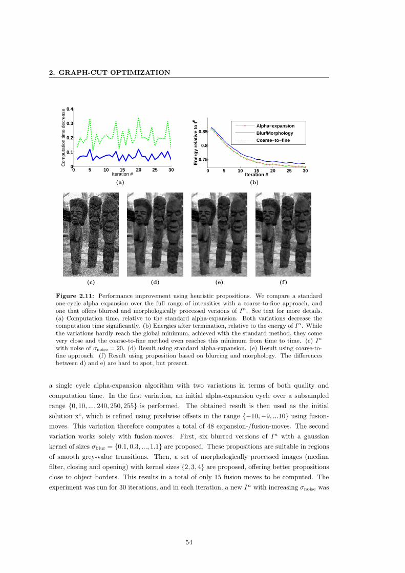
2. GRAPH-CUT OPTIMIZATION
0 5 10 15 20 25 300
0.1
0.2
0.3
0.4
Iteration #
Com
puta
tion
time
decr
ease
(a)
0 5 10 15 20 25 30
0.75
0.8
0.85
Iteration #
Ene
rgy
rela
tive
to I
n
Alpha−expansion
Blur/Morphology
Coarse−to−fine
(b)
(c) (d) (e) (f)
Figure 2.11: Performance improvement using heuristic propositions. We compare a standardone-cycle alpha expansion over the full range of intensities with a coarse-to-fine approach, andone that offers blurred and morphologically processed versions of In. See text for more details.(a) Computation time, relative to the standard alpha-expansion. Both variations decrease thecomputation time significantly. (b) Energies after termination, relative to the energy of In. Whilethe variations hardly reach the global minimum, achieved with the standard method, they comevery close and the coarse-to-fine method even reaches this minimum from time to time. (c) In
with noise of σnoise = 20. (d) Result using standard alpha-expansion. (e) Result using coarse-to-fine approach. (f) Result using proposition based on blurring and morphology. The differencesbetween d) and e) are hard to spot, but present.
a single cycle alpha-expansion algorithm with two variations in terms of both quality and
computation time. In the first variation, an initial alpha-expansion cycle over a subsampled
range {0, 10, ..., 240, 250, 255} is performed. The obtained result is then used as the initial
solution xc, which is refined using pixelwise offsets in the range {−10,−9, ...10} using fusion-
moves. This variation therefore computes a total of 48 expansion-/fusion-moves. The second
variation works solely with fusion-moves. First, six blurred versions of In with a gaussian
kernel of sizes σblur = {0.1, 0.3, ..., 1.1} are proposed. These propositions are suitable in regions
of smooth grey-value transitions. Then, a set of morphologically processed images (median
filter, closing and opening) with kernel sizes {2, 3, 4} are proposed, offering better propositions
close to object borders. This results in a total of only 15 fusion moves to be computed. The
experiment was run for 30 iterations, and in each iteration, a new In with increasing σnoise was
54

2.3 Graph-Cuts for Multi-Label Problems
generated. Each variation starts with the noisy image as its initial solution x0. In addition,
the order in which the propositions were offered were randomly selected, which generally offers
slightly better results than iterating linearly over the set of labels1.
As can be expected, the computation time compared to the standard, one-cycle alpha-
expansion approach is reduced by about 80% for the first variation (48/256 ≃ 0.19%), while
the second variation runs roughly 20 times faster (15/256 ≃ 0.06%). Figure 2.11a shows the
running times for each iteration, relative to the time of the standard, one-cycle alpha-expansion.
In Figure 2.11b, a plot of the energy ratio between the original noisy image In and the final
energies are plotted for each iteration. The second variation performs noticeably worse (but still
only by 1%) than the one-cycle full alpha-expansion. However, the first variation’s energy comes
very close to the global minimum, in some iterations even reaching it. A similar observation
can be made by looking at the images from one of the iterations. Figure 2.11c shows the noisy
input image In with σnoise = 20. Figures 2.11d-f show the result of the standard one-cycle
alpha-expansion, the coarse-to-fine and the blur/morphology variations, respectively. Visual
differences are difficult to spot, but present.
Conclusion
We can conclude this section with the fact that move-making algorithms allow a greater flex-
ibility, and require much less memory than transformation methods. While transformation
methods are able to find the global minimum of certain energy functions, the strong local
minima obtained with move-making algorithms are usually very close to the global minimum.
While this cannot be theoretically proven, and the theoretical upper bound of alpha-expansions
is quite far away from the optimum, the results of the first experiment show that reaching the
global minimum, at least for submodular terms, is possible. In addition, the large number of
vertices and edges needed by transformation methods will not generally lead to faster results
than can be obtained with iterative move-making algorithms (see algorithm complexities in
Section 2.2.1.2). Furthermore, memory requirements grow exponentially with the number of
labels, which prevents the applicability to problems with large label sets (which we will need
for the registration algorithms in Chapter 3 and 4). Higher-order energy functions (also used
in Chapters 3 and 4), reduced to pairwise terms, are generally partly non-submodular and
can also not be expressed using Equation (2.11) (there exists no pairwise ωpq, and E(xp, xq) of
Equation (2.11) only depends on the label combination, whereas reduced higher-order functions
depend both on the specific variables of the clique, as well as on the clique’s label combination,
which both are not of pairwise nature). The map compositing algorithms proposed in this thesis
cannot be represented either as convex pairwise terms (needed for (Ish03)), nor in the form of
Equation (2.11) (ωpq depends on the label combination as well).
1This has no effect on the one-cycle standard alpha-expansion, as it converges to the global minimum, butproduces slightly better results for the two other variations (BVZ01).
55

2. GRAPH-CUT OPTIMIZATION
Having justified the preference of move-making algorithms compared to transformation
methods, a second conclusion can be made. When the label set is significantly large, huge im-
provements regarding the computation time are possible by selecting propositions in a fusion-
move approach. However, such heuristic selection requires careful adaptation to the specific
energy function to prevent significant loss in the quality of the results. Global minima are still
possible with such approaches, but as not as likely as with standard alpha-expansion.
2.4 Graph-Cuts for Image Registration and Map Compositing
2.4.1 Image Registration using Graph-Cuts
As was discussed in Chapter 1, the algorithm being in the center of the cartography process
is the registration of partly overlapping images. Several contributions have been devoted to
formulating this problem in terms of discrete energy minimization. This section will outline the
basic ideas of these works. In Section 2.5, we will conclude this chapter with an initial proof-of-
concept that uses a sparse graph structure to efficiently register overlapping cystoscopic images.
The energy of a non-rigid deformation field can be written as
E(xi→j) =∑
p∈V
Edatap (xp) + λ
∑
(p,q)∈N8
Eregpq (xp, xq), (2.13)
where now the configuration xi→j : V → L ⊂ R2 corresponds to 2D displacement vectors,
estimated for each pixel p in the source (floating) image Ii : V → {0, ..., 255}. The data term
measures the similiarity of pixels p in the source image to sub-pixels p + xp in the target
(reference) image Ij : R2 → {0, ..., 255}1:
Edatap (xp) = D (Ii(p), Ij(p+ xp)) . (2.14)
The choice ofD in Equation (2.14) is application specific. In (TC07), a simple squared difference
between observed intensity values Ii(p) and Ij(p+ xp) was used. The authors of (SC10) use a
mutual information based data term.
The regularization term of Equation (2.13) used in (TC07, SC09, SC10) penalizes the first
derivative in the displacement field
Ereg(xp, xq) = ‖xp − xq‖2 . (2.15)
To allow user interaction, landmarks were included to Equation (2.13) by the authors of
(LSC07). Pixels declared as a landmark add hard constraints to the energy function, as these
1Grey-values at sub-pixel locations Ij(x+xp) are obtained via bi-cubic interpolation and Dirichlet boundaryextension.
56

2.4 Graph-Cuts for Image Registration and Map Compositing
pixels must be transformed as indicated by the user. Other pixels are influenced by nearby land-
marks based on their Euclidean distance. In (LSC07), on images from a coronary angiogram,
the registration converges to an incorrect local minimum without landmarks, but converges to
the correct solution when adding them. While this landmark-based approach can be helpful
in the case of strong, non-linear deformations, it is not feasible on a large image database or
video-sequence due to the exhaustive amount of user interaction needed. However, it could be
added in a semi-automatic setup, where registration results are checked automatically for their
reliability, and only unreliable image pairs are sent to the user after processing the entire image
sequence.
As the computation time increases linearly with the size of the label set L, a multi-level
approach was proposed in (SC09). Starting from the coarsest level (lowest resolution) in a
Gaussian pyramid, an alpha-expansion based image registration algorithm is applied to the
images until convergence with a reduced label set. The result (the labeling representing the
displacement at the current level) is propagated up (resized) to the next level, and this scheme
continues until the finest (original) level of the pyramid is reached.
In comparison to a “direct” registration of the source and target images, the pyramidal ap-
proach leads to a processing time reduction of 54%, whereas the data superimposition robustness
and accuracy are similar for both approaches. This result shows the potential of multi-scale
approaches with graph-cut optimization. However, the time needed to superimpose two images
(538 seconds on average) for the multi-scale approach of (SC09), with L = {0,±1, ...,±17}2,
also shows that dense1 graph-cut based registration with a large two-dimensional label set
leads to high processing times, which is not feasible for the registration of a video-sequence
that contains hundreds or thousands of images.
This issue can be overcome using the methods proposed in (GKT+08). Displacements of
control points in a regular grid (instead of dense representation) are optimized via MRFs, which
leads to a dimensionality reduction on the variables. Registration costs are still computed on the
entire image domain via non-linear interpolation of the control point displacements. The authors
also apply a multi-scale coarse-to-fine scheme, and are able to estimate the displacement field in
10-50 seconds2 (depending on the similarity measure used) on 256× 256 pixel image resolution.
However, this method assumes that an initial pre-alignment (translation and rotation) has been
performed beforehand, greatly reducing the search space encapsulated in L. In Section 2.5, we
also use a set of control points to reduce the number of variables, but these points are selected
based on image texture. This allows to compute registration costs without interpolation on the
entire image domain, leading to faster registration times. At the same time, no pre-alignment
is required, allowing to directly estimate the underlying image transformations.
Proposed in (GHN+10), second-order cliques, obtained from triangulated meshes, allow
to compute (local) image (dis-)similarity using affine approximations. This approach is more
1Here, dense means that each pixel is represented by a vertex in the graph.2C++ program running on a 2.16 GHz CPU.
57

2. GRAPH-CUT OPTIMIZATION
robust than pixel-wise similarity measurements in texture-homogeneous image regions, and in-
variant to affine transformations (as opposed to block matching approaches, which are only
invariant to translations). Like the method of (GKT+08), triangulated meshes greatly reduce
the number of variables, but the higher-order potentials infer more complexity on MRF opti-
mization.
Graph-Cuts for Stereo and Optical Flow Estimation
While there exist only a few publications (see previous section) specifially contributed to image
registration (superimposing two images as best as possible) using discrete energy minimization,
the energy formulation of stereo or optical flow estimation in terms of discrete energy mini-
mization is closely related to non-rigid registration. In both applications, the minimized energy
should correspond to the most probable displacement field that maps pixels of the source image
onto their displaced position in the target image. However, optical flow results are used for mo-
tion or object segmentation, not explicitly for image superimposition. Similar, stereo disparity
estimation is used to obtain the depth of a scene, visualized by two (or more) cameras from
different viewpoints. Consequently, the problems one faces and the attempts to solve them are
significantly different between optical flow and image registration/superimposition. In stereo
or optical flow estimation, one faces the problem of occlusions, photometric inconsistencies,
large displacements of foreground objects with respect to the movement of the background, or
the preservation of thin object structures. On the other hand, cystoscopic image registration
algorithms do not pose the problem of occlusions or large displacements of foreground objects
(apart from small tissues flowing along the FOV, which have to be ignored, not matched).
However, they must be able to register images accurately under strongly varying image condi-
tions (see again Section 1.3 for details). While stereo and optical flow methods usually have a
large amount of image overlap, cystoscopic image pairs may overlap by less than 50%, requiring
careful attention to be paid to border conditions.
A detailed listing of corresponding publications regarding optical flow and stereo estimation
would therefore go beyond the scope of this thesis, even though the Middlebury Stereo and
Optical Flow databases1 contain several contributions based on graph-cuts, which were, at the
time of their publication, among the top performing methods ((LRR08, GHN+10) represent two
interesting approaches). The evaluation pages of these websites are therefore a good starting
point to explore various approaches towards stereo and optical flow methods.
2.4.2 Map Compositing using Graph-Cuts
The last step of the cartography process consists of composing the globally aligned images into
a single global textured map. Unlike classical blending/interpolation methods (see Section 3.4),
formulating this goal as an MRF optimization problem can overcome the issue of blurring and
1http://vision.middlebury.edu/stereo/, http://vision.middlebury.edu/flow/
58

2.4 Graph-Cuts for Image Registration and Map Compositing
ghosting. This approach allows to optimize the location of “hard” transitions between overlap-
ping images, instead of (non-)linear interpolation between the images in superimposed areas.
Pairwise MRFs were first used in (KSE+03b) to optimize texture synthesis between overlap-
ping images. Given N (usually superimposed) images, the configuration x : V→ {0, ..., N − 1}
assigns each pixel p in the map an image index xp, which determines the grey/color value to
be used for the texture of the map. In other words, the color of a pixel in the map is selected
among all images in which this pixel is visible, with the aim to optimize the visual quality in
the map. Optimal transitions are obtained by minimizing a sum of pairwise potential costs
E(x) =∑
(p,q)∈N
Ep,q(xp, xq)
with Ep,q(xp, xq) = T (xp 6= xq)Γ(Ixp
(p), Ixq(q)),
where Γ(·) measures the dissimilarity across image transitions (where xp 6= xq). This idea was
extended by several combinations of unary and pairwise potential functions in (ADA+04). The
authors refer to this approach by “Interactive Digital Photomontage”, and via user interaction,
several problems are addressed. Examples are selective composites, where the user selects best
elements in several images of a changing scene, and the composed map shows the optimal fusion
of these images.
The idea of (KSE+03b, ADA+04) was extended to the problem of texturing triangulated
three-dimensional surfaces in (LI07). Vertices represent faces of the surface mesh, and pairs of
vertices represent faces which share a common edge. Unary potentials capture the “quality” of
a face being textured by its projection in the image Ixp, while pairwise potentials again penalize
dissimilarities across image transitions.
All approaches (KSE+03b, ADA+04, LI07) assume image exposure and white balance not to
vary too drastically, and remove any remaining exposure differences via gradient-domain fusion
(ADA+04) or seam levelling (LI07) in a second step after initial seams have been obtained. An
exception is the “relighting” technique of (ADA+04), where the images are taken under differ-
ent unknown lighting conditions, but the images are expected to be perfectly aligned. Both
assumptions do not hold in a cystoscopic cartography application, as images differ strongly
in terms of exposure and are usually slightly misaligned due to local bladder movements.
At the same time, the quality of each image varies strongly. In Chapter 3, we modify the
ideas proposed in (KSE+03b, ADA+04, LI07) to optimize contrast, texture alignment, and
exposure/white-balance differences for cystoscopic video-sequences. This approach is extended
to three-dimensional cartography in Chapter 4.
59

2. GRAPH-CUT OPTIMIZATION
Figure 2.12: Pig bladder phantom used in (HSB+09) for the accuracy evaluation. (a) Originalhigh resolution picture. The simulated transformations are illustrated with the successive imagepositions and their shapes. (b) Map obtained with the method of (MLDB+08). (c) Map obtainedwith the method of (HMBD+10). In both maps, local registration errors accumulate and lead toto misaligned structures at several map positions.
2.5 Sparse Graph-Cuts for Cystoscopic Image Registration: a
Proof of Concept
2.5.1 Cystoscopic Image Registration Assessment
This section will show preliminary developments regarding the possibility/potential of graph-cut
based optimization approaches towards the registration of cystoscopic video-sequences. First,
results of existing state-of-the-art registration methods for cystoscopic image registration are
presented. A comparison with these results will show the potential of an initial assessment of
graph-cut based image registration in Section 2.5.3. In a comparative study (HSB+09), the
methods of (MLDB+08, HMBD+10), described in Section 1.3.3.2, were compared in terms of
accuracy, robustness and computation time. This comparison was performed with a realistic
phantom consisting of images simulating a cystoscopic video-sequence. A pig bladder (which
is visually very similar to human bladder tissue1) was incised, opened and put flat on a table
to capture a high resolution photograph of it. This photograph was used to simulate known
transformations that typically occur during a cystoscopic examination, and to obtain a ground
truth cystoscopic image sequence. To do so, a sequence of sub-images were extracted from
the digital high resolution picture. The simulated perspective transformations are visible on
Figure 2.12a2. They are symbolized by the displacement and shape change of consecutive
images, which are drawn onto the bladder picture and represent the camera movement.
1Even experienced urologists state that pig bladder texture is visually very close to human bladders.2While color images are used in Chapters 3 and 4, previous registration algorithms do not incorporate color
information. The comparison in this chapter is therefore performed on grey-level images.
60

2.5 Sparse Graph-Cuts for Cystoscopic Image Registration: a Proof of Concept
(a) (b) (c)
Figure 2.13: Image registration using dense graph-cuts. (a) and (c) Input images, geometricallylinked by a pure in-plane rotation. (b) Result using the authors’ implementation of (TC07). Forvisualization purposes, only for each 5th vertex, an arrow is drawn. The resulting flow field issmooth, and produces a mean local registration error of ǫi→i+1 = 0.06 pixels. This shows thatgraph-cuts are well suited for cystoscopic image registration in terms of registration accuracy.However, the large label set (all possible 2D displacements) leads to a computation time of severalminutes, unsuitable for large video-sequences.
To assess registration accuracy, the mean local registration error is defined as
ǫi→i+1 =1
|V|
∑
p∈V
||T2Di→i+1p− T2D
i→i+1p||, (2.16)
where T 2Di→i+1 and T 2D
i→i+1 are respectively true (known) and estimated homographies placing
pixels from the coordinate system of image Ii into the coordinate system of image Ii+1. Fig-
ures 2.12b-c show the final map composed by the methods of (MLDB+08) and (HMBD+10)
respectively. While local errors1 are small, they accumulate to large errors and result in visible
misalignments when the sequence returns to the first image, clearly visible by comparing with
Figure 2.12a (in Figures 2.12b-c, a visible seam is present at the top left hand side, and the
vascular structure in the bottom left hand side is positioned incorrectly due to the accumulating
registration errors).
2.5.2 Cystoscopic Image Registration using Standard Graph-Cuts
A method, similar to that described in (TC07) and defined in Equation (2.13), was implemented
and tested for assessing the adequacy of graph-cut techniques to register cystoscopic images.
The data terms consist of squared intensity differences, and the regularization penalizes the
first derivative in the displacement vector field, as defined in Equation (2.15). The method
produces small local registration errors (mean registration error ǫi→i+1 less than 0.2 pixels)
1 It is recalled that local errors or local homographies refer to registration errors or transformations betweenconsecutive images, while global errors are the cartography errors due to placement (with the global homography)of image Ii in the global map coordinate system (typically that of the first image).
61

2. GRAPH-CUT OPTIMIZATION
on all perspective transformations tested on the phantom of Figure 2.12a. These small errors
allow to assume that graph-cuts can be a well suited approach when image registration quality
(accuracy) is the main goal. Figure 2.13 shows two input images geometrically related by a pure
in-plane rotation, which becomes visible through the computed dense vector flow xi→j shown
in Figure 2.13b. The registration time of several minutes is similar to that of (MLDB+08),
but far higher than the two seconds needed to superimpose the images with the method of
(HMBD+10). As discussed in Chapter 1, the computation time is the least important aspect,
as the maps are mainly used for surgery planning and follow-up examinations. Even if is
desirable to build panoramic maps shortly after the examination, or even in real-time, map
construction accuracy and robustness remain the most important evaluation criteria for the
registration quality. Any improvements made towards a possible real-time usage must therefore
not sacrifice this registration quality.
2.5.3 Sparse Graph-Cuts with Locally Refined Vertex and Edge Selection
In order to obtain T2Di→j , it is not necessary to compute a dense deformation field, but only
a few homologous pixel positions (at least 4) are needed to estimate a homography (recall
Section 1.3.2 for the estimation of T2Di→j from a set of homologous points). A sparse sampling
Vs ⊂ V in image Ii : V→ {0, ..., 255} can speed up the computation time significantly. However,
more attention needs to be paid to the data term evaluation. Indeed, when data terms are only
computed for sparsely sampled vertices, the optimization is likely to converge to a poor local
minimum because the implicit influence of neighboring pixels in a dense sampling V is lost. To
reduce loss of information, data terms must be more robust and should consider the intensity
distribution of a local neighborhood of each vertex. Therefore, the original pixelwise squared
difference is now measured in an 11x11 squared window centered on each vertex p:
Esparsep (xp) =
∑
p′∈N11p
|Ii(p′)− Ij(p
′ + xp)|2.
Again, Ij : R2 → {0, ..., 255} and grey-values at sub-pixel locations are obtained via bi-cubic
interpolation and Dirichlet boundary conditions. As will be shown in Section 2.5.4, this vertex
sub-sampling reduces the computation time by some orders of magnitude.
However, as can be seen from Figure 2.14b, where a “winner-takes-all” result is shown (in
other words, optimization with λ = 0), data terms show several outliers (displacement vectors
which significantly deviate from their true displacement) when an equally spaced grid Vs is
used. This observation complicates convergence towards the global minimum, and is due to the
fact that an equidistant sub-sampling will place many vertices into regions with poor intensity
variations (almost homogeneous). Indeed, if such regions are selected in the source image by the
vertex subsampling, they can be “matched” with several regions in the target image containing
similar homogeneous intensity values. This situation often arises in cystoscopic bladder images.
62

2.5 Sparse Graph-Cuts for Cystoscopic Image Registration: a Proof of Concept
(a) (b) (c)
Figure 2.14: (a) Dense displacement vector field of Figure 2.13a used as reference. (b) The use ofa sub-sampled grid of vertices speeds up the computation by some orders of magnitude. However,data terms become less distinctive and show several outliers, making convergence towards theenergy minimum more complicated (reprojection error ǫi,i+1 = 2.91 pixels including regularizationterm). (c) Using the proposed vertex selection scheme (WDBH+na), where potential locations arecomputed using the Harris corner detector (HS88) and thinned using ANMS (BSW05), verticesare locally moved to more distinctive locations. This improves the data terms, reduces outliers,and leads to a reprojection error of ǫi→i+1 = 0.26.
The idea of the proposed algorithm is to prefer image regions with more texture in order to
facilitate the registration, while still retain a sparse set of vertices.
To obtain more discriminative data terms, vertices are locally moved to positions with
more texture. To do so, possible vertex positions are first determined with the Harris corner
detector (HS88). The response map threshold is set low to obtain key-points also in (almost)
homogeneous image regions. Then, these points are thinned using Adaptive Non-Maximal
Suppression (ANMS), see (BSW05). The strongest key-point (strongest response of the Harris
detector) is first selected, and all key-points in a fixed radius around it are removed from the
list. Then, the second strongest key-point is selected, and the process is iterated until no more
key-points can be removed. This locally refined sampling Vs ensures that key-points are well
spread over the image (due to the low threshold), while locally, they are positioned at the most
discriminative locations, such as those corresponding for example to vascular structures. This
vertex selection scheme is illustrated in Figure 2.15a, and its improvement regarding the data
terms can be seen in Fig 2.14c (now “winner-takes-all” shows less outliers, thereby facilitating
a correct minimum).
The neighborhood system for the selected vertices can be obtained with a k-nearest neighbor
approach, or by looking in a fixed radius around each vertex. The drawback of the latter
approach is that the significance of the interaction term varies for each vertex depending on
the number of neighbors within the radius. Consider for example a vertex that is more likely
to be labeled incorrectly, then the interaction penalty for assigning a false label will be less
expensive when it has only a few distant neighbors, and zero when it is not close to other
vertices. On the other hand, the k-nearest neighbor approach can result in an edge system with
63

2. GRAPH-CUT OPTIMIZATION
(a) (b)
Figure 2.15: Sparse Graph-Cut method. (a) Nodes selected using Harris corner detector andAdaptive Non-Maximal Suppression. (b) Neighborhood system based on the seeded watershedtransform. An edge is added to the graph between two nodes if the influence zones correspond to8-connected neighbors.
(a)
φ = 10◦ Sx = Sy = 1.2 φ = 5◦, Sx = Sy = 1.1(tx, ty) = (−4, 3)
Dense 0.06 0.02 0.09Sparse, Harris 0.26 0.26 0.24Sparse, equally 2.91 0.94 1.51
(b)
Figure 2.16: (a) I - III Input images used to evaluate the performance differences between dense,equally rastered and Harris-ANMS-based vertex selection. (b) Comparison of mean registrationerrors, as given by Equation (2.16). Applied image transformations (parameters of Equation (1.4))are given in the first line of the table. The errors are measured in pixels.
holes. Therefore, we propose a neighborhood system that takes the spatial distribution of the
selected vertices into account. Using the selected vertices as basins, the watershed transform
(Soi03) computes the influence zone of each vertex. These influence zones can be used to
generate a natural neighborhood system for the vertices. Figure 2.15b illustrates this approach.
The neighborhood system Ns consists of all vertex pairs whose influence zones are 8-connected
64
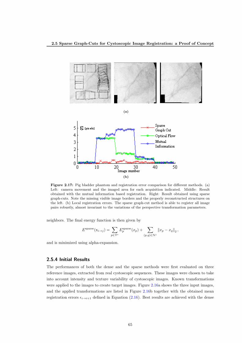
2.5 Sparse Graph-Cuts for Cystoscopic Image Registration: a Proof of Concept
(a)
(b)
Figure 2.17: Pig bladder phantom and registration error comparison for different methods. (a)Left: camera movement and the imaged area for each acquisition indicated. Middle: Resultobtained with the mutual information based registration. Right: Result obtained using sparsegraph-cuts. Note the missing visible image borders and the properly reconstructed structures onthe left. (b) Local registration errors. The sparse graph-cut method is able to register all imagepairs robustly, almost invariant to the variations of the perspective transformation parameters.
neighbors. The final energy function is then given by
Esparse(xi→j) =∑
p∈Vs
Esparsep (xp) +
∑
(p,q)∈Ns
‖xp − xq‖2 ,
and is minimized using alpha-expansion.
2.5.4 Initial Results
The performances of both the dense and the sparse methods were first evaluated on three
reference images, extracted from real cystoscopic sequences. These images were chosen to take
into account intensity and texture variability of cystoscopic images. Known transformations
were applied to the images to create target images. Figure 2.16a shows the three input images,
and the applied transformations are listed in Figure 2.16b together with the obtained mean
registration errors ǫi→i+1 defined in Equation (2.16). Best results are achieved with the dense
65
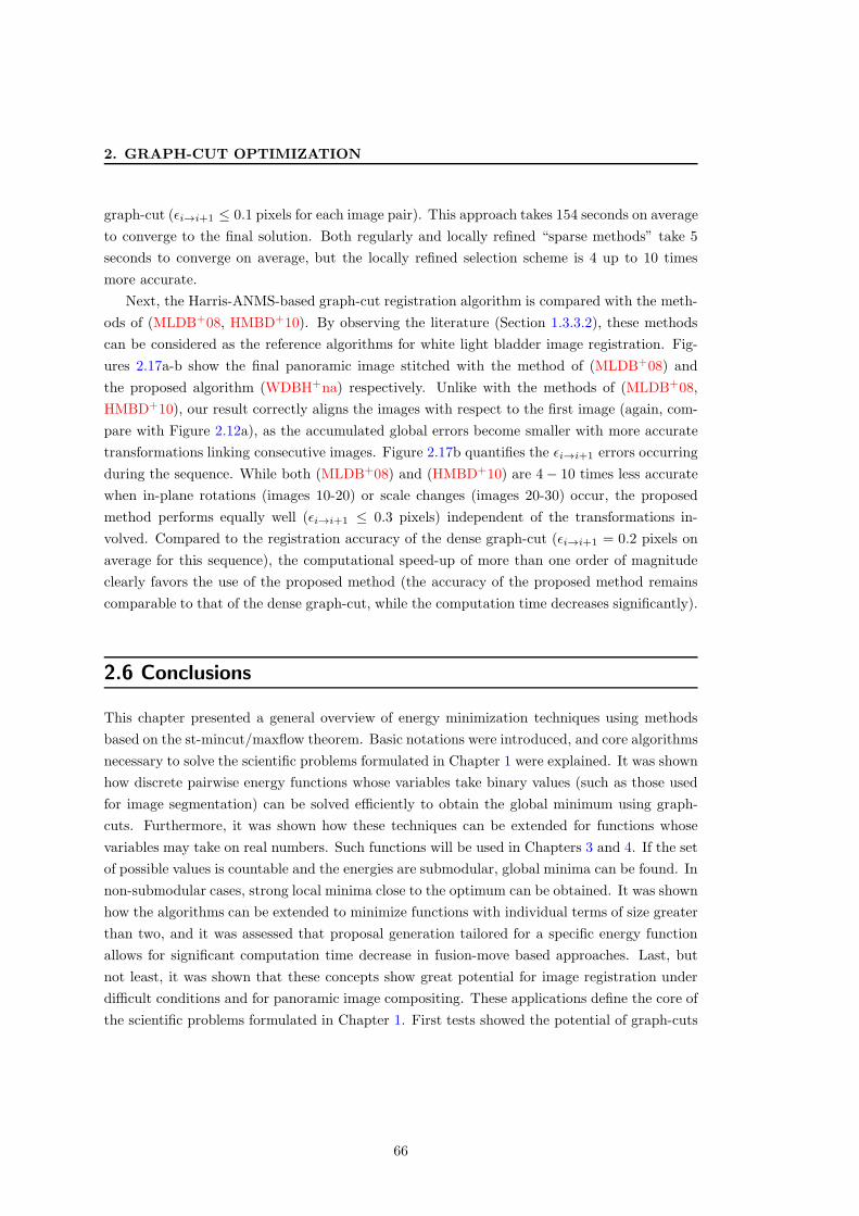
2. GRAPH-CUT OPTIMIZATION
graph-cut (ǫi→i+1 ≤ 0.1 pixels for each image pair). This approach takes 154 seconds on average
to converge to the final solution. Both regularly and locally refined “sparse methods” take 5
seconds to converge on average, but the locally refined selection scheme is 4 up to 10 times
more accurate.
Next, the Harris-ANMS-based graph-cut registration algorithm is compared with the meth-
ods of (MLDB+08, HMBD+10). By observing the literature (Section 1.3.3.2), these methods
can be considered as the reference algorithms for white light bladder image registration. Fig-
ures 2.17a-b show the final panoramic image stitched with the method of (MLDB+08) and
the proposed algorithm (WDBH+na) respectively. Unlike with the methods of (MLDB+08,
HMBD+10), our result correctly aligns the images with respect to the first image (again, com-
pare with Figure 2.12a), as the accumulated global errors become smaller with more accurate
transformations linking consecutive images. Figure 2.17b quantifies the ǫi→i+1 errors occurring
during the sequence. While both (MLDB+08) and (HMBD+10) are 4− 10 times less accurate
when in-plane rotations (images 10-20) or scale changes (images 20-30) occur, the proposed
method performs equally well (ǫi→i+1 ≤ 0.3 pixels) independent of the transformations in-
volved. Compared to the registration accuracy of the dense graph-cut (ǫi→i+1 = 0.2 pixels on
average for this sequence), the computational speed-up of more than one order of magnitude
clearly favors the use of the proposed method (the accuracy of the proposed method remains
comparable to that of the dense graph-cut, while the computation time decreases significantly).
2.6 Conclusions
This chapter presented a general overview of energy minimization techniques using methods
based on the st-mincut/maxflow theorem. Basic notations were introduced, and core algorithms
necessary to solve the scientific problems formulated in Chapter 1 were explained. It was shown
how discrete pairwise energy functions whose variables take binary values (such as those used
for image segmentation) can be solved efficiently to obtain the global minimum using graph-
cuts. Furthermore, it was shown how these techniques can be extended for functions whose
variables may take on real numbers. Such functions will be used in Chapters 3 and 4. If the set
of possible values is countable and the energies are submodular, global minima can be found. In
non-submodular cases, strong local minima close to the optimum can be obtained. It was shown
how the algorithms can be extended to minimize functions with individual terms of size greater
than two, and it was assessed that proposal generation tailored for a specific energy function
allows for significant computation time decrease in fusion-move based approaches. Last, but
not least, it was shown that these concepts show great potential for image registration under
difficult conditions and for panoramic image compositing. These applications define the core of
the scientific problems formulated in Chapter 1. First tests showed the potential of graph-cuts
66

2.6 Conclusions
to register images with high accuracy, independent of the transformation that geometrically
links overlapping image pairs.
Contributions
• Established a state-of-the-art literature on discrete energy minimization techniques us-
ing graph-cuts, with a particular focus on problems typical of cystoscopic cartography
applications.
• Determined that fusion-moves benefit from significant computation time reduction with-
out noticeable quality decrease if propositions are generated smartly and adapted to the
specific energy function.
• Initial implementation and proof of concept that show the potential of graph-cuts regard-
ing cystoscopic cartography. Accurate results outperforming state-of-the art methods
were achieved and the algorithm performs independently of the geometric transformation
linking overlapping images.
• A novel locally refined vertex and edge selection scheme for graph-cut based image reg-
istration. This allowed to reduce the computation time of image registration by two
orders of magnitude, without significant loss in registration accuracy, independent of the
geometric transformation relating overlapping images.
Publication
• T. Weibel, C. Daul, A. Ben Hamadou, D. Wolf, and R. Rosch. Endoscopic bladder image
registration using sparse graph cuts. In 17th IEEE International Conference on Image
Processing (ICIP), pages 157–160, September 2010. Hong Kong, China (oral presentation)
67

2. GRAPH-CUT OPTIMIZATION
68

Chapter 3
2D Cartography
In the previous chapter, it was shown that graph-cuts can be a promising registration technique
for white light cystoscopic video-sequences. Accuracy and robustness of consecutive image
registration using graph-cut methods are superior to those of the tested state-of-the-art methods
(MLHMD+04, MLDB+08, HMBD+10). On the phantom cystoscopic video-sequence provided
by (HSB+09), the accuracy remains relatively constant independent of the parameter values of
the perspective transformation linking consecutive images.
3.1 Problem Description and Chapter Overview
Despite the initial improvements on image registration accuracy, errors still accumulate visibly
during image placement in a common coordinate system. This fact remains a problem, even
for registration methods more accurate than that proposed in the previous chapter. This is
particularly true for clinical data, since the phantom data of (HSB+09) used in the evaluation
of Section 2.5.4 leads to registration errors much smaller than observed with patient data. As
clinicians regularly return to previously visited locations on the bladder surface during the
examination, this will lead to visible and strong misalignments.
Figure 3.1a shows this effect on a sequence where the cystoscope trajectory performs a loop.
Apart from brightness gradients due to exposure differences and vignetting, the superimposition
of consecutive images leads to visually coherent texture transitions in image regions without
closing or crossing endoscope trajectories. However, when observing the first and last image
of the sequence (indicated by the red and green quadrangles in Figure 3.1a), the global mis-
alignment is evident, both in scale and spatial position. This is illustrated in the top image of
Figure 3.1b, where both first and last images are superimposed (these images should be perfectly
superimposed when registration errors during the sequence are 0). In order to provide visually
coherent panoramic images, these errors need to be detected and corrected automatically.
69

3. 2D CARTOGRAPHY
(a) (b)
(c) (d)
Figure 3.1: Effects of accumulated cartography errors and map improvements presented in thischapter. (a) While superimposed consecutive images show visually coherent transitions (exceptfor exposure and vignetting induced brightness gradients), accumulated errors lead to visiblemisalignments when the instrument returns to previously visited locations on the bladder surface.This is indicated by the red (first image of the sequence) and green (last image) quadrangles, whichare visibly misaligned. (b) Top: first and last image superimposed before correction. Bottom:after correction, the images are now correctly superimposed. (c) Map after correcting globalmisalignments. Small texture misalignments may still be present due to the non-planar surfaceand local warping. Furthermore, images suffering from motion blur decrease the visual quality ofthe map. (d) Stitching techniques can correct small misalignments, increase the contrast of thepanoramic map, and remove blending induced gradients. The contrast in d) is strongly enhanced,and exposure/texture gradients are removed, as can be seen by comparing with with c).
70

3.1 Problem Description and Chapter Overview
State-of-the-art contributions devoted to bladder cartography have not presented methods
to detect accumulated errors, and usually show maps without loop trajectories or crossing paths.
An exception is (MLDB+08), where the authors have proposed a method to correct global mis-
alignment by jointly adjusting the local transformations between first and last image of a loop
using a steepest gradient optimization. However, they present no method to automatically de-
tect these loops, and their algorithm cannot be easily extended to multiple overlapping images
(the adjustment is only performed on consecutive images). Feature-correspondence based ap-
proaches (e.g. (BBS+10)) could directly employ traditional methods of globally registering the
entire sequence using bundle-adjustment techniques (see (Sze06) for an introductory overview).
The advantage of feature based methods lies both in the fast image pair registration and in the
possible automatic detection of non-overlapping images. However, as discussed in Chapter 1, in
the white light modality, iconic data registration must be used for robust image superimposi-
tion, which impedes registering all possible pairs of the sequence (as required for classic bundle
adjustment) due to time constraints.
The effects of error accumulation can also be understood by comparing Figure 3.1a with the
corrected map (corrected image positions in the map) of Figure 3.1c. Figure 3.1c is visually
more coherent in terms of texture discontinuities, even if small texture misalignments remain.
In this corrected map, the first and last images are adequately superimposed, as shown in the
bottom image of Figure 3.1b. The remaining texture misalignments are due to the spherical
bladder surface projected onto a flat panoramic coordinate system1, local warping of the surface
due to physical contact to other organs, and bending of the bladder caused by the movement
of the rigid cystoscope. These small texture misalignments can be corrected by finding optimal
seam locations between overlapping images. As opposed to blending techniques, seams depict
a hard border between parts of partly overlapping images. For misaligned texture, the former
approach leads to ghosting and blur, while seams allow for sharp transitions. Such seams may
also be used to increase the contrast of the map (by discarding blurry images), as shown in
Figure 3.1d.
To sum up Figure 3.1, the map correction proposed in this thesis consist of two steps:
the first step corrects small misalignments and maximizes the texture contrast in the map.
Exposure differences are then corrected in a second step, while retaining the obtained contrast
of step one.
The remainder of this chapter is organized as follows. While the chronological order of the
proposed cartography pipeline starts with the registration of consecutive image pairs, we will
first explain the proposed method to detect a meaningful subset of non-consecutive image pairs
in Section 3.2. These will then be used to globally correct accumulated cartography errors.
In Section 3.3, higher-order cost functions that are invariant to perspective transformation
parameter values will be presented. In addition, a coarse-to-fine minimization scheme that
1As will be shown in Chapter 4, without additional information, such as the distance of the instrumentfrom the surface, the parametric surface model cannot be used as a-priori information for registration or surfacecompositing.
71

3. 2D CARTOGRAPHY
allows to reduce computation time significantly is proposed. This registration algorithm will
be used for both consecutive and non-consecutive image pairs. For consecutive image pairs, it
leads to more accurate and robust solutions. For non-consecutive image pairs, the proposed
terms authorize a successful registration where other methods fail. Lastly, a combined stitching
and exposure correction technique is proposed in Section 3.4. It allows to correct small local
texture misalignments (remaining after global correction in Section 3.2) and is able to create
visually coherent panoramic images with minimal loss of information (maximum contrast).
These different algorithm steps are evaluated in Section 3.5, both quantitatively on realistic
phantom data, as well as qualitatively on patient data. In addition, we demonstrate that
the proposed algorithms may also be used in more traditional applications, such as seamless
stitching of a set of images captured with consumer cameras, or high dynamic range image
composition.
Parts of this chapter previously appeared in (WDWRum, WDW+12, WDW+an).
3.2 Global Map Correction
Feature correspondence based algorithms (e.g. such as the one presenteded in(BBS+10)) are
fast, so registering all possible image pair combinations of a sequence is possible within appli-
cation time limits (i.e. shortly after the examination). If all pairs of images with a minimum
overlap could be registered in a robust fashion, rejecting non-overlapping pairs would be sim-
ple. A rejection criterion could be a minimum percentage (threshold) of inlier matches after
RANSAC fitting. All valid feature correspondences between overlapping image pairs could then
be used to compute global transformations using bundle adjustment techniques (Sze06). In such
an approach, global transformation matrices are adjusted by minimizing the sum of distances
between homologous pixel positions in all registered image pairs.
However, as was justified in Chapter 1, feature correspondences cannot be robustly estimated
in the white light modality. Iconic data registration methods are slower than feature based ap-
proaches and therefore registering all possible image pair combinations requires too much com-
putation time. To overcome this problem, we propose to use the initial global transformations
T2D0→i (placing the images in the global map coordinate system) obtained by concatenating local
transformations T2Di→i+1 between consecutive pairs to detect overlapping non-consecutive image
pairs (i, j 6= i+1) automatically. From these overlapping additional image pairs, a useful subset
must be selected and registered1. The computed additional transformations T2Di→j 6=i+1 can then
be used to correct accumulated errors globally. Global transformations must be adjusted so
that local registration errors (for all computed T2Di→j) are minimized, which leads to visually
coherent superimposition.
1Again, due to time constraints, the registration of all available overlapping image pairs is infeasible.
72

3.2 Global Map Correction
To sum up, the method detailed in this section is a bundle adjustment method. The dif-
ference to classical methods is that, instead of using all image pair combinations, only an
automatically selected subset of image pairs needs to be registered, and no image primitives
have to be extracted from the images. This subset of image pairs is then used during the
iterative and global map correction process.
3.2.1 Detecting Additional Image Pairs
Once all local transformations T2Di→i+1 between consecutive images are computed, the global
matrices T2D0→i relating each image Ii with the coordinate system of a reference image can be
obtained by concatenation. For simplicity (and without loss of generality), we will use the first
image (I0) as the reference image:
T2D0→i =
i−1∏
k=0
T2Dk→k+1. (3.1)
This straightforward approach (a global matrix is a simple product of consecutive local matrices)
yields visually coherent maps (MLDB+08, HMBD+10, BBS+10, WDBH+na) between consec-
utive images. However, small registration errors accumulate, and when the cystoscope comes
back to previously visited locations (e.g. when a loop is closed or during a “zig-zag”-path), the
misalignment is evident (see again Figure 3.1b). In order to correct these misalignments, the
local transformations between non-consecutive but overlapping image pairs need to be taken
into account when computing global transformations T2D0→i. Using the initial map constructed
with Equation (3.1) as a starting point, we can estimate the overlap ratio δ2Di,j between any two
(consecutive and non-consecutive) image pairs (Ii, Ij) of the sequence using:
δ2Di,j = min
(Ai,j
Ai.Ai,j
Aj
)
, (3.2)
In Equation (3.2), Ai,Aj are the areas in pixels of the transformed images Ii and Ij in the
panoramic image (i.e. the map coordinate system), and Ai,j is the area of overlap in pixels
between images Ii and Ij . Areas Ai and Aj are computed by perspective warping of quadrangles
into the global coordinate system, and Ai,j is computed using the area of polygon overlap (i.e.
Ai ∩Aj). For two completely superimposed images, δ2Di,j = 1, while for non-overlapping image
pairs, δ2Di,j = 0. Theoretically, we could compute T2Di→j for all pairs of images with an overlap δ2Di,j
greater than a minimally allowed overlap tδ (i.e. δ2Di,j > tδ). This is however computationally
expensive and therefore not recommended for iconic data based registration algorithms. Instead,
a greedy algorithm similar to (MFM04) allows us to select a meaningful subset of possible
additional image pairs ((i, j) : δ2Di,j > tδ, j 6= i + 1). We create a weighted, undirected initial
graphG = (V,E,w) in which every image Ii is represented by a node vi, and existing consecutive
73

3. 2D CARTOGRAPHY
Algorithm 1: Determining additional image pairs.
Input: Overlap threshold tδ, short-cut threshold tϑOutput: Indices of additional transformation pairs S// Set of initial (i.e. consecutive) pair indicesSc ← {(i, j) : j = i+ 1};// Set of non-consecutive indicesSnc ← {(i, j) : j > i+ 1};S ← ∅;// Compute overlap for all pairsforeach (i, j) ∈ Sc ∪ Snc do
compute δ2Di,j ;
// Remove non-consecutive pairs with too low overlapSnc ← Snc\{(i, j) : δ2Di,j < tδ};
while Snc 6= ∅ doCreate G(E, V, w) from Sc;// Compute material shortcutforeach (i, j) ∈ Snc do
compute ϑi,j ;
// Discard pairs with ϑi,j < tϑSnc ← Snc\{(i, j) : ϑi,j < tϑ};// Add pair with largest ϑi,j to the set of additional pairs ...S ← S ∪ {(i, j) : max(ϑi,j)};// ... and remove it before the next iteration.Snc ← Snc\{(i, j) : max(ϑi,j)};// Update combined set (consecutive and additional pair indices)Sc ← Sc ∪ S;
transformations T2Di→i+1 will create an edge ei,i+1 with weight wi,i+1 = 1−δ2Di,i+1 that links nodes
vi and vi+1. Let the “material shortcut” be
ϑi,j = 1−wi,j
∑
i j w,
where∑
i j w is the sum of image overlap along the shortest path from vi to vj , found using
Dijkstra’s algorithm (Dij59). Note that for consecutive pairs (i, i + 1), ϑi,i+1 is always 0,
while it is close to 1 for pairs whose shortest path spans many images. At each iteration of
the proposed algorithm, we add a new edge ei,j (again with weight wi,j = 1 − δ2Di,j ) to G for
the pair with the highest ϑi,j . Adding the image pair with the highest “material shortcut”
ensures that accumulated errors can be attenuated for a large number of images (i.e. many
images can be reached using a significantly shorter path after adding ei,j to G). In the next
iteration, ϑi,j is then recomputed for all remaining pairs ((i, j) : δ2Di,j > tδ). These steps are
repeated until no pairs with a minimum amount of “material shortcut” tϑ are left. A schematic
overview of the algorithm is given in Algorithm 1. The final graph then consists of edges
between consecutive image pairs (for which the transformations are already computed), and
74

3.2 Global Map Correction
edges between additional, non-consecutive image pairs. Before continuing with the next section,
these image pairs must be registered using the methods that will be explained in Section 3.3.
3.2.2 Bundle Adjustment
Both consecutive and non-consecutive local transformation matrices T2Di→j can now be combined
to obtain the best possible global matrices T2D0→i. Similar to Section 3.2.1, we construct a
weighted graph G = (E, V, w) using all available transformations. The weights are defined as
wi,j =1
|T2Di→j(Ii)|
∑
p∈T2Di→j
(Ii)
∥∥Ij(p)− T2D
i→j(Ii)(p)∥∥2
2,
and represent the mean sum of squared differences (SSD, divided by the number of valid
pixel positions |T2Di→j(Ii)|) of the colors of homologous pixels between image Ij and image
T2Di→j(Ii), i.e. image Ii transformed into the coordinate system of Ij . A color difference is
given by the Euclidean distance between two RGB vectors, and the mean SSD is obtained
by dividing the sum of all distances by the number of homologous pixels. The pre-processing
method used in (HMBD+10) is applied before computing the weights wi,j , so that the SSD is
not biased by different levels of exposure or vignetting. We observed that images differing in
contrast have less influence on the mean SSD (due to the pre-processing step applied) than small
registration inaccuracies have. Thus, using the mean SSD as the edge weights will ensure that
when several paths with comparable numbers of transformations are available for computing
the global transformation for an image, the one with the best overall registration quality is
chosen. The global transformation T2D0→i for each image Ii is then obtained by concatenation
along the shortest path in G.
While this reduces the accumulated error for each image that has “shortcut”-transformations
(e.g. loops will now be closed, see Figure 3.1a), smaller local errors still remain. Consider for
example consecutive images (Ii, Ii+1) that have a different shortest path to the reference image
I0. This implies independently accumulated errors when placing Ii and Ii+1 into the global
map. These errors are corrected using a modified bundle adjustment algorithm, similar to that
presented in (MFM04). A regularly spaced grid of points G that covers the entire map is created.
If two overlapping images (Ii,Ij) are perfectly aligned in the reference coordinate system, their
local transformation T 2Di→j should be equal to the product of their global transformations, i.e.
T2Di→j = T2D
0→jT2D0→i
−1. This property allows to create the cost function
E =∑
g∈G
1
|Lg|
∑
i,j∈Lg
∥∥∥g − T2D
0→j
−1T2D
i→jT2D0→ig
∥∥∥2
, (3.3)
which can be minimized using non-linear least squares. In Equation (3.3), g is a grid point of
the set G, and Lg is the set of image pairs for which a local transformation T2Di→j exists and g
75
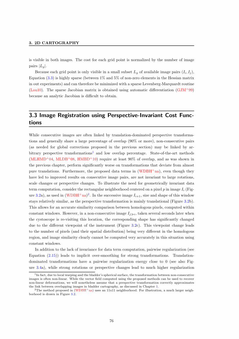
3. 2D CARTOGRAPHY
is visible in both images. The cost for each grid point is normalized by the number of image
pairs |Lg|.
Because each grid point is only visible in a small subset Lg of available image pairs (Ii, Ij),
Equation (3.3) is highly sparse (between 1% and 5% of non-zero elements in the Hessian matrix
in out experiments) and can therefore be minimized with a sparse Levenberg-Marquardt routine
(Lou10). The sparse Jacobian matrix is obtained using automatic differentiation (GJM+99)
because an analytic Jacobian is difficult to obtain.
3.3 Image Registration using Perspective-Invariant Cost Func-
tions
While consecutive images are often linked by translation-dominated perspective transforma-
tions and generally share a large percentage of overlap (90% or more), non-consecutive pairs
(as needed for global corrections proposed in the previous section) may be linked by ar-
bitrary perspective transformations1 and low overlap percentage. State-of-the-art methods
(MLHMD+04, MLDB+08, HMBD+10) require at least 90% of overlap, and as was shown in
the previous chapter, perform significantly worse on transformations that deviate from almost
pure translations. Furthermore, the proposed data terms in (WDBH+na), even though they
have led to improved results on consecutive image pairs, are not invariant to large rotations,
scale changes or perspective changes. To illustrate the need for geometrically invariant data
term computation, consider the rectangular neighborhood centered on a pixel p in image Ii (Fig-
ure 3.2a), as used in (WDBH+na)2. In the successive image Ii+1, size and shape of this window
stays relatively similar, as the perspective transformation is mainly translational (Figure 3.2b).
This allows for an accurate similarity comparison between homologous pixels, computed within
constant windows. However, in a non-consecutive image Ij≫i, taken several seconds later when
the cystoscope is re-visiting this location, the corresponding shape has significantly changed
due to the different viewpoint of the instrument (Figure 3.2c). This viewpoint change leads
to the number of pixels (and their spatial distribution) being very different in the homologous
region, and image similarity clearly cannot be computed very accurately in this situation using
constant windows.
In addition to the lack of invariance for data term computation, pairwise regularization (see
Equation (2.15)) leads to implicit over-smoothing for strong transformations. Translation-
dominated transformations have a pairwise regularization energy close to 0 (see also Fig-
ure 3.4a), while strong rotations or perspective changes lead to much higher regularization
1In fact, due to local warping and the bladder’s spherical surface, the transformation between non-consecutiveimages is often non-linear. While the vector field computed using the proposed methods can be used to recovernon-linear deformations, we will nonetheless assume that a perspective transformation correctly approximatesthe link between overlapping images in bladder cartography, as discussed in Chapter 1.
2The method proposed in (WDBH+na) uses an 11x11 neighborhood. For illustration, a much larger neigh-borhood is drawn in Figure 3.2.
76

3.3 Image Registration using Perspective-Invariant Cost Functions
(a) (b) (c)
Figure 3.2: Data terms determined in rectangular image regions are not invariant to perspec-tive transformations. (a-b) Consecutive images of a cystoscopic video-sequence. The geometrictransformation relating these images is mainly translational, so that a fixed shape window (redrectangles) can be used to compare similarity between homologous pixels. (c) Image taken afterthe cystoscope has returned to a previously visited location. The instrument is now significantlycloser and has a different orientation towards to the bladder surface, as indicated by the quadranglethat corresponds to those of a) and b).
energies (Figure 3.4b), even though both transformations are valid representations of the un-
derlying transformation model (see Equation (1.4)). Therefore, data and regularization terms
must be invariant to the geometric transformations linking partly overlapping cystoscopic im-
ages.
3.3.1 Data Term
As illustrated in Figure 3.2, measuring homologous image region similarity independently of
the underlying projective transformation is not possible using constant window regions. Indeed,
the window’s geometry (in the target image Ij) would have to be adapted to the given trans-
formation T2Di→j , which of course is not known in advance. However, higher-order terms allow
to incorporate shape into the energy function itself. First introduced in (GHN+10), second-
order terms can be used to compare image similarity in triangular texture patches located in
the source and target images. Let △p,q,r be a triangular shape defined by vertices p, q and r,
and let △p′,q′,r′ be the corresponding triangular shape defined by p′ = p+ xp, q′ = q + xq and
r′ = r + xr. Then these two triangles are related by an affine transformation T2D△
pqr , and any
position u inside △p,q,r can be mapped to its corresponding (sub-pixel) position inside △p′q′r′
via T2D△
pqr u. This enables to compare image similarity for arbitrary affine transformations T2Di→j
77

3. 2D CARTOGRAPHY
relating Ii and Ij . The data terms are then computed using
E△(xi→j) =∑
(p,q,r)∈C△
E△pqr(xp, xq, xr) with
E△pqr(xp, xq, xr)=
1
|△pqr |
∑
u∈△pqr
∥∥∥Ii(u)−Ij(T
2D△
pqr u)∥∥∥2,
(3.4)
where the set of cliques C△ consists of triplets located in a regularly spaced grid Vr ⊂ V, and
Ii : V → R3. Colors Ij(x + xp) at sub-pixel locations are obtained via bi-cubic interpolation
and Dirichlet boundary conditions, so Ij : R2 → R
3. Each E△pqr(xp, xq, xr) is normalized by the
number of discrete sample positions |△pqr | inside △pqr . The geometric relationship between
△pqr and △p′q′r′ for different types of transformations is illustrated in Figure 3.3. While the
geometric transformation relating the entire images Ii and Ij is usually projective (i.e. not
globally affine), if the triangles are made sufficiently small, the perspective transformation
T2Di→j can be approximated by several locally affine transformations T2D△
pqr .
There is however a drawback since too small (i.e. too numerous) triangles will lead to many
of them lying in homogeneous areas (i.e. with poor texture information), making the data
terms less distinctive. On the other hand, too large triangles will impede the correct estimation
of the fully projective transformation and lead to globally affine approximations. This issue is
illustrated in Figure 3.3. As long as the images are only related by translations, rectangular
windows, as used in (WDBH+na), are sufficient (see Figure 3.3b). The triangular data terms
allow to compute an exact similarity for rigid and affine transformations (see Figure 3.3c-d).
However, when the underlying transformation is fully projective, triangular data terms will
only allow for an approximative data comparison, as illustrated in Figure 3.3e. While the three
triangle vertices are perfectly transformed using the affine approximation, positions inside the
triangles are misplaced because the actual transformation is fully projective. This can be seen
when comparing the position of the triangle’s center (intersection of the three blue lines) in
Figure 3.3a and Figure 3.3e.
Therefore, we propose an extension to the idea of (GHN+10). Third-order terms can be used
to compute a similarity between quadrangular neighborhood shapes, allowing fully perspective
transformations:
E�(xi→j) =∑
(p,q,r,s)∈C�
E�pqrs(xp, xq, xr, xs) with
E�pqrs(xp, xq, xr, xs)=1
|�pqrs|
∑
u∈�pqrs
∥∥∥Ii(u)−Ij(T
2D�
pqrs u)∥∥∥2.
(3.5)
The set of of cliques C� consists of quadruples, located in the same regularly spaced grid
Vr than used for C△. Again, each E�pqrs(xp, xq, xr, xs) is normalized by the number of discrete
sample positions |�pqrs| inside the quadrangle�pqrs. The fully projective geometric relationship
between �pqrs and �p′q′r′s′ allows to set the size of the quadrangles tailored to white light
78

3.3 Image Registration using Perspective-Invariant Cost Functions
(a) (b) (c) (d) (e)
Figure 3.3: Invariance of data term windows. (a) Artificial source image Ii. (b) Target image Ij ,related to Ii by pure translations. The rectangular window (red) is invariant to transformations,so it is sufficient to compare image similarity. (c) Ij , related to Ii by a rigid 2D transformation.The rectangular window is no longer sufficient. However, the affine transformation that warpsthe triangular vertices from Ii to Ij can be used to compute the similarity exactly. (d) Affinetransformation relating Ii and Ij . Triangular windows are also sufficient to compute an invariantdata term. (e) Fully projective transformation. While the three triangular vertices are perfectlytransformed onto Ij using the affine approximation, positions inside the triangle are incorrectlytransformed. This can be seen at the intersection of the blue lines (which meet at the center ofthe green triangle), which is at a different position than in a)-d).
cystoscopic images (e.g. large enough to include textured areas in all quadrangles), without
risking affine approximations to T2Di→j .
The set of cliques C△ (Equation (3.4)) and C� (Equation (3.5)) are selected from the regular
grid Vr, which is illustrated in Figure 3.7, together with the regularization cliques defined in
the next section. A 10× 10 grid is used for the experiments in Section 3.5.
3.3.2 Regularization Term
Pairwise regularization terms are generally well suited to obtain energy minima without outliers.
Intuitively, they penalize strong displacement vector differences between neighbouring vertices,
therefore leading to smooth displacement fields:
E↔(xi→j) =∑
(p,q)∈Nr
1
‖p− q‖2‖xp − xq‖
22, (3.6)
where ‖·‖22 is the squared L2 norm1 of the difference of displacement vectors assigned to vertices
p and q. The neighborhood system Nr corresponds to the 8-connectivity in Vr, as shown in
Figure 3.7. However, when T2Di→j consists of displacements of large magnitude and deviates from
pure translations, even smooth displacement vector transitions between neighbouring vertices
will contribute significantly to the energy cost. This phenomenon is illustrated in Figure 3.4.
Consecutive images are related by transformations of small magnitude and dominated by trans-
lations. Figure 3.4a shows one such image pair. For this example, the average pairwise cost
value between vertex pairs, computed with Equation (3.6), is 3.2. The total pairwise regu-
larization energy contributes only by small fraction to the entire energy, allowing the energy
1The L1 norm is better suited when discontinuities in the displacement vector field are expected (e.g. dueto moving objects or depth discontinuities), which is not the case in cystoscopy.
79

3. 2D CARTOGRAPHY
(a) (b)
Figure 3.4: Varying regularization influence on the global cost function. (a) Visual representationof the estimated transformation between consecutive images. The relative small regularizationenergy (3.2 on average per vertex pair) due to the low magnitude of the translation-dominateddisplacements. (b) Illustration of the estimated transformation between non-consecutive images.The pairwise regularization energy is two orders of magnitude larger (313.7 on average) than thatof a) due to the strong perspective relationship between the images.
minimum to correspond to optimal superimposition of the iconic data. This is not the case
for many non-consecutive image pairs, such as the one shown in Figure 3.4b. The average
regularization energy per vertex pair is by two orders of magnitude larger (313.7 per pair) than
for the image pair shown in Figure 3.4a, and the total regularization energy contributes signif-
icantly to the entire energy. This is equivalent to an implicit over-regularization compared to
transformations of moderate magnitude, and will lead to piecewise constant displacement fields
in homogeneous (i.e. without texture) areas (see Figure 3.5c). Because in such areas, data
terms are not very distinctive (i.e. return similar costs for several possible displacements), a
locally constant displacement field (with a local regularization cost of 0) is less expensive than
smooth transitions. In cases of severe transformations, the implicit over-regularization may
even prevent a correct estimation.
Again, higher-order terms can be used to overcome this problem. Regularization should
penalize displacement fields that deviate from the perspective transformation model, indepen-
dent of magnitude of the dominant perspective transformation parameters of Equation (1.4).
This can be achieved by using a fourth-order regularization term. Consider four vertices
k, l,m, n ∈ Vr and their corresponding locations k′, l′,m′, n′ induced by the displacement vector
field xi→j . These four correspondences exactly define a perspective transformation T2D♦
klmn. The
following regularization cost is then computed:
E♦(xi→j) =∑
(p,k,l,m,n)∈C♦
E♦pklmn(xp, xk, xl, xm, xn) with
E♦pklmn(xp, xk, xl, xm, xn) =
∥∥∥T2D♦
klmnp− (p+ xp)∥∥∥
2
2.
(3.7)
To ensure that this regularization has effect on all vertices jointly, the vertices (k, l,m, n) are
fixed as the four corner vertices in Vr. All remaining vertices p will then form a fourth-order
clique (p, k, l,m, n) ∈ C♦. As all of these cliques share the same four reference vertices, the set
80
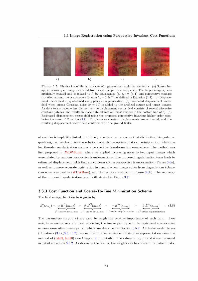
3.3 Image Registration using Perspective-Invariant Cost Functions
a) b) c) d)
Figure 3.5: Illustration of the advantages of higher-order regularization terms. (a) Source im-age Ii, showing an image extracted from a cystoscopic video-sequence. The target image Ij wasartificially created and is related to Ii by translations (tx, ty) = (5, 1) and perspective changes(rotation around the cystoscope’s X -axis) hx = 2.5e−4, as defined in Equation (1.4). (b) Displace-ment vector field xi→j obtained using pairwise regularization. (c) Estimated displacement vectorfield when strong Gaussian noise (σ = 30) is added to the artificial source and target images.As data terms become less distinctive, the displacement vector field consists of several piecewiseconstant patches, and results in inaccurate estimation, most evident in the bottom half of c). (d)Estimated displacement vector field using the proposed perspective invariant higher-order regu-larization term of Equation (3.7). No piecewise constant displacements are estimated, and theresulting displacement vector field conforms with the ground truth.
of vertices is implicitly linked. Intuitively, the data terms ensure that distinctive triangular or
quadrangular patches drive the solution towards the optimal data superimposition, while the
fourth-order regularization ensures a perspective transformation everywhere. The method was
first proposed in (WDWRum), where we applied increasing noise to two input images which
were related by random perspective transformations. The proposed regularization term leads to
estimated displacement fields that are conform with a perspective transformation (Figure 3.6a),
as well as to more accurate registration in general when images suffer from degradations (Gaus-
sian noise was used in (WDWRum), and the results are shown in Figure 3.6b). The geometry
of the proposed regularization term is illustrated in Figure 3.7.
3.3.3 Cost Function and Coarse-To-Fine Minimization Scheme
The final energy function to is given by
E(xi→j) = α E△(xi→j)︸ ︷︷ ︸
2nd-order data term
+ β E�(xi→j)︸ ︷︷ ︸
3rd-order data term
+ γ E↔(xi→j)︸ ︷︷ ︸
1st-order regularization
+ δ E♦(xi→j)︸ ︷︷ ︸
4th-order regularization
. (3.8)
The parameters (α, β, γ, δ) are used to weigh the relative importance of each term. Two
weight-parameter sets are used according the image pair type to be registered (consecutive
or non-consecutive image pairs), which are described in Section 3.5.2. All higher-order terms
(Equations (3.4),(3.5),(3.7)) are reduced to their equivalent first-order representation using the
method of (Ish09, Ish10) (see Chapter 2 for details). The values of α, β, γ and δ are discussed
in detail in Section 3.5.2. As shown by the results, the weights can be constant for patient data.
81

3. 2D CARTOGRAPHY
0 2 4 6 8 10 12 140
5
10
σn
ε
4th order 1st order
(a)
0 2 4 6 8 10 12 140
5
10
σn
ε
4th order1st order
(b)
Figure 3.6: Effect of the perspective invariant higher-order regularization term. For both a)and b), the x -axis denotes the standard deviation σn of the noise added to the images, while they-axis represents the registration error ǫ. The error measure ǫ is the mean difference betweenthe estimated displacement vectors and their position as induced by a perspective transforma-tion. (a) With increasing noise level applied to source (Ii) and target (Ij) images, the estimatedtransformation T2D
i→j deviates more and more from the perspective transformation fitted on thedisplacement vector field (blue crosses). Using the proposed higher-order regularization term, theobtained displacement vector field is always conform with a perspective transformation (red cir-cles). (b) This also leads to statistically more accurate registration when computing ǫ using theground truth transformation. In Equation (3.15), ǫ is properly defined.
The energy of Equation (3.8) can be minimized using alpha-expansion (Section 2.3.1) and
the BHS algorithm (Section 2.2.3). However, the set of potential displacement vectors is very
large. For consecutive image pairs, the overlap can be expected to be no less than 90%. Even
then, this corresponds to displacements of 40 pixels, which in turn leads to a label set
L = {(−40,−40), (−40,−39), ..., (40, 39), (40, 40)} .
This would require the computation of |L| = 6561 st-mincuts for one cycle of alpha-expansion.
In addition, the higher-order terms add a significant amount of auxiliary variables to the graph.
The computation time for one image pair would range in multiples of ten minutes, clearly not
suitable for a video-sequence with many hundreds of images. Non-consecutive image pairs may
have percentages of overlap less than 50% and stronger transformations, leading to much larger
label sets. Therefore, to allow for a second diagnosis some minutes after the examination, a
coarse-to-fine energy minimization scheme is required to reduce the computation time.
Image Pyramids
First, the input (source and target) images Ii and Ij are sub-sampled kmax times to form
two image pyramids, where levels kmax and k1 correspond to the original resolution and the
lowest resolution, respectively. The size of an image Iki at level k corresponds to a fraction
of ωk = 0.7kmax−k of the original image resolution. Images at level k are obtained by first
applying a Gaussian low-pass filter to the original input images (at level kmax). The kernel size
σk for the filter is determined with the formula σk = 1.6/(2ωk), which is known to produce very
little discretization artefacts (MY09). The image is then resized by the factor ωk using bilinear
82

3.3 Image Registration using Perspective-Invariant Cost Functions
Figure 3.7: Graph structure used for image registration. Black dots represent the regular gridV
r. Dashed grey lines show vertex pairs for which the first-order regularization costs are evaluated(Equation (3.6)). Green lines illustrate a higher-order clique for which the perspective enforcingregularization term (Equation (3.7)) is computed. The red triangle shows a triplet of vertices forwhich the second-order data term (Equation (3.4)) is computed. If fully perspective data termsneed to be computed, the vertex connected to the triangle by a dashed red line forms a third-orderclique with the triangle vertices (Equation (3.5)).
interpolation. The number of images in the pyramids directly influences the computation
time, as only the coarsest level is searched for the entire range of expected displacements
r1 = rmaxωk, with rmax being the largest magnitude of expected displacement vectors. For
the remaining levels in the pyramid, the range of displacements rk is strongly reduced. When
fewer pyramid levels are chosen, computation time will increase. If too many levels are chosen,
the minimization might get trapped in a poor local minima at (very low resolution) level k1.
We will discuss the choice of level numbers in more detail in Section 3.5. Figure 3.8 shows an
example of an image pyramid with kmax = 4.
Minimization Scheme
The minimization starts at the coarsest level with an initial solution (displacement vector
field) xk=1. For easier notation, we use x = xi→j . This solution is created from an initial
guess of the underlying geometric transformations. For consecutive image pairs, the initial
83

3. 2D CARTOGRAPHY
(a) (b) (c) (d)
Figure 3.8: Image pyramid illustration with kmax = 4. From (a) lowest resolution at level k = 1to (d) original image resolution at level k = kmax.
Algorithm 2: Coarse-to-fine minimization scheme
Input: Initial T2Di→j
Output: Final T2Di→j
Create x1 from T2Di,j ;
for k = 1 to kmax doxk ← xk;repeat
for (rx, ry)T ∈ [−rk : 1 : rk,−rk : 1 : rk]
T do
xPk ← xk + (rx, ry)T ;
xk ← Fuse(xPk , xk);
until convergence ;xk ← xk;if k < kmax then
xk+1 ← Upsample(xk) ;
T 2Di→j ← LeastSquares(xkmax);
guess is the identity matrix1, while for non-consecutive image pairs, it is created using the
initial global transformations T2D0→j
−1T2D
0→i, which are computed using Equation (3.1) after
all consecutive transformations have been estimated. Based on this initial guess, a region of
interest is determined, and within this region, the set of vertices Vr is selected. The region of
interest consists of vertices which have a displacement vector pointing to a valid position in Ij .
The steps of the coarse-to-fine scheme are illustrated in Algorithm 2 and described below.
The initial solution is then iteratively refined using fusion moves until convergence. Propo-
sitions xPk are created by adding a set of constant 2D displacement offsets to each element of xk.
The initial magnitude of these offsets is determined by the maximal displacement magnitude r1
that may relate Ii and Ij . For consecutive images, r1 = 75ω1 pixels is used. Non-consecutive
images may be related by much larger displacements, so r1 = 250ω1 pixels is chosen. The final
1Here, one could also choose the transformation estimated from the previous image pair, or predict thetransformation using a Kalman filter. This may decrease computation time, but has no effect on registrationaccuracy and robustness, as own tests have shown.
84

3.4 Contrast-Enhancing Map Compositing
solution xk after each level is then up-scaled to the next level in the pyramid, where it serves
as the input xk+1. Again, a region of interest is then computed to select the vertices. For the
remaining pyramid levels k = 2, ..., kmax, rk is independent of the underlying transformation
fixed to rk = 21. Finally, the solution obtained on the original resolution is then used in a least
squares estimation to compute T2Di→j (see Section 1.3.2).
3.4 Contrast-Enhancing Map Compositing
Once all global transformations T2D0→i have been estimated, the final textured map can be
created by superimposing the N images on a global planar surface (map coordinate system
V). For simplicity, in the remainder of this section, it is assumed that the images are already
transformed into the global coordinate system, i.e.
Ii = T2Di→0(Ii), ∀i ∈ {0, ..., N − 1}.
Previous contributions either perform this superimposition directly (MLHMD+04, MLDB+08,
BRM+09), i.e. by overwriting the map image by image, or perform (non-)linear blending
techniques to remove/minimize vignetting and exposure related artifacts (WRS+05, HMBD+10,
BGS+10). If all images are perfectly aligned and of the same (visual) quality, these approaches
will work well. However, as stated in the first section of this chapter, the globally transformed
images may still show small misalignments due to local warping of the bladder surface, and in
general due to the spherical shape of the bladder projected onto a planar surface. Even after
the global map correction of Section 3.2, these small misalignments remain. Additionally, many
images suffer from motion blur or de-focus and significantly decrease the visual appearance of
the map. Blending techniques therefore, while leading to visually pleasing panoramic images
at the first glance, in fact reduce contrast of the underlying images by linearly interpolating
between slightly misaligned overlapping parts and by ignoring the images’ quality.
The aim of this section is to correct the effects of these small misalignments, while increasing
contrast and visual quality of the map. The proposed algorithm consists of two steps, which
are formulated as energy minimization problems and solved using graph-cuts:
• First, optimal borders in regions defined by overlapping image parts are determined.
These borders, which we refer to as seams, are classically used to suppress texture mis-
alignments by choosing transitions where textured structures (e.g. blood vessels) overlap
(where misaligned structures intersect). In addition, we extend the graph-cut formulation
to include a cost function based on the images’ quality, so that pixels in contrasted im-
ages are preferred over pixels in blurry images. Unlike previous contributions to bladder
1Sub-pixel accuracy can easily be integrated by setting the step size to a non-integer value (e.g.[−rk : 0.5 : rk] in Algorithm 2) at the expense of increasing computation time. As triangle or quadrangle cliquesare already computing image dissimilarity at sub-pixel levels, we found that this did not increase registrationaccuracy noticeably.
85

3. 2D CARTOGRAPHY
cartography, no blending (linear interpolation between overlapping images) is performed,
leading to much more contrasted panoramic images with higher visual quality.
• Then, in the second step, exposure and vignetting related color gradients across the
previously found seams are removed. This is achieved without blending (blurring), so
that the contrast obtained using the previous step is retained.
3.4.1 Seam Localization
Unlike images for which classical seam detection methods (KSE+03b, ADA+04) are usually
adapted, overlapping images extracted from cystoscopic video-sequences vary significantly in
levels of exposure due to the instrument’s auto-exposure mode and varying distance to the
bladder surface. These differences introduce a strong bias to the optimal seam placement in
the classical energy functional. Indeed, a seam connecting a strongly exposed region in one
image with a less bright peripheral region in another image induces strong brightness gradients,
even if the images are precisely aligned. This in turn will prevent accurate (e.g. seamless)
superimposition of vascular structures when the images are slightly misaligned. Since these
vascular structures represent only a small percentage of the entire image texture, misaligned
vascular structures contribute much less to the overall energy cost than exposure differences
do. This bias is illustrated in Figure 3.9c. The general idea of the proposed method is to favor
seam positions in image regions with constant colors/brightness so that textures (e.g. vascular
structures) have a non negligible impact (in comparison to color gradients) during the seam
detection. The advantage of this idea is twice: on the one hand texture discontinuities can
be minimized and misaligned vascular structures can be seamlessly stitched, and on the other
hand the contrast of the map can be maximized.
As brightness gradients, due to exposure and vignetting, typically correspond to low fre-
quency changes, the seam localization is applied in the high-pass frequency domain by creating
high-pass filtered versions of the input (original) images:
Ihpi = Ii − Ii ⋆ Gσ, ∀i ∈ {0, ..., N − 1}, (3.9)
where ⋆ denotes the convolution operator, and Gσ the Gaussian convolution kernel. As illus-
trated in Figure 3.9d, these filtered images effectively ensure that seam positions are not biased
by low frequency gradients. Thus, by minimizing an appropriate energy function, vascular
structures can be optimally superimposed (e.g. coherently aligned), even if they are slightly
misaligned in the overlapping images. This energy function is written as
Eseam(x) = λseam
∑
(p,q)∈N8
Eseampq (xp, xq) +
∑
p∈V
Eseamp (xp), (3.10)
where x : V→ {0, ..., N − 1} assigns an image index to each pixel in the map. In other words,
the color for a pixel p is to be taken from the image Ixp. Correct alignment of vascular structures
86

3.4 Contrast-Enhancing Map Compositing
(a) (b)
(c) (d)
(e) (f)
Figure 3.9: Seam detection and exposure correction. (a)-(b) Two input images, (mis-)alignedin a common coordinate system. (Mis-)aligned here means that the images represent globallytransformed images affected by errors (as for bladder images, the image superimposition is usuallynot perfect after the registration, so that small texture discontinuities remain visible in the globalmap). The error in this example is much larger than for bladder maps for illustration purposes.Vignetting and different levels of exposure is visible. (c) Images overlaid in the red and greenchannel. The strong exposure difference impedes finding appropriate seam locations. (d) Like c),but using high-pass-filtered images. Potential costs of seams are strongly diminished (i.e. greypixels) after filtering, except at positions where the object boundaries do not overlap. (e) Seamsfound using the images of d). (f) After exposure correction.
87

3. 2D CARTOGRAPHY
is encapsulated in the regularization term
Eseampq (xp, xq) =
∥∥∥Ihpxp
(p)− Ihpxq(q)∥∥∥
2
2· T (xp 6= xq), (3.11)
which minimizes gradients along seam lines. As always, T (·) is equal to 1 if its argument is
true, else 0. This formulation, similarly used in (KSE+03b, ADA+04), will prefer seams in
homogeneous areas (e.g. each connected vascular structure is preferably taken from a single
image). If structures are not completely observed in a single image, the seam will likely go
through the intersecting region, in case the images do not perfectly align this structure.
However, blurry images tend to be preferred, as the gradients between those is less strong
than between contrasted images. This leads to a loss in contrast in the final map. In order
to retain as much information from the video-sequence as possible, we introduce a contrast-
enhancing data term, formally given by
Eseamp (xp)=exp
−
maxp′∈N11
p
Ihpxp(p′)− min
p′∈N11p
Ihpxp(p′)
maxp′∈N11
p
Ihpxp(p′) + min
p′∈N11p
Ihpxp(p′)
. (3.12)
This term computes the contrast in image Ixpusing Michelson’s formula in an 11x11 neighbor-
hood N11p for a pixel p. A high contrast corresponds to well a focused image and leads to a low
energy, and vice-versa.
Equation (3.10) is minimized via alpha-expansion until convergence. The pairwise terms
(Equation (3.11)) are not necessarily submodular with regard to alpha-expansion. While
Epq(α, α) is always equal to zero, Epq(xp, xq) may be larger than Epq(xp, α) + Epq(α, xq) at
some point. However, the number of non-submodular terms is very small (always less than
0.1%, but mostly exactly 0%) in all experiments, so the BHS algorithm drives the solution to
a strong local minimum.
3.4.2 Exposure and Vignetting Correction
Minimizing Equation (3.10) ensures that vascular structures are seamlessly superimposed (even
if the images are initially not perfectly aligned). In addition, loss of information is minimized
by preferring contrasted images over blurry ones. When applying the obtained solution (image
index xp for each pixel p ∈ V) to the original images, stitching induced color gradients due
to exposure and vignetting are strongly noticeable (see Figure 3.9e). These effects can be
significantly attenuated using blending techniques (see again Section 1.3.4). However, classical
blending methods affect the contrast and seamless alignment obtained by the method of the
previous section. Instead, exposure related differences (across seams) must be removed while
retaining contrast and alignment. Removing these differences should also not lead to drastic
(and unnatural) color appearance changes. This last constraint can be formulated using the
following data term:
Eexpp (mp) =
∥∥∥∥
Ixp(p)
||Ixp(p)||
−mp
||mp||
∥∥∥∥2
, (3.13)
88

3.5 Results
where now the solution m : V → L ⊂ Rn assigns n-dimensional color vectors mp (n = 3 for
RGB color space) to each pixel p in the map. Equation (3.13) ensures that a color vector mp
points in the same direction1 (in the n-dimensional color space) than the original color vector of
the input image Ixp(p), as given by the solution x of Equation (3.10) obtained in the previous
step. Since the intensities of colors may change without penalty, but strong changes in hue and
saturation are penalized, the natural aspect of the epithelium is preserved. Removing color
gradients along the previously determined seam lines (i.e. when xp 6= xq) should also ensure
that the contrast of the original images is retained. This is achieved by penalizing gradient
differences within connected image segments (e.g. when xp = xq):
Eexppq (mp,mq) = (T (xp = xq)·||Ixp
(p)−Ixq(q)|| − ||mp −mq||)
2,
where T (·) equals 1 when its arguments are true, and 0 otherwise. Combining both exposure
correction terms leads to the following energy function:
Eexp(m) =∑
p∈V
Eexpp (mp) + λexp
∑
(p,q)∈N4
Eexppq (mp,mq), (3.14)
where the use of the N4 is necessary, as previous seams were determined using the complemen-
tary N8. If both seam detection and exposure correction were based on the same connectivity,
certain exposure differences could not be corrected without inferring new ones. Equation (3.14)
is iteratively minimized using fusion-moves. In each iteration, the propositions mp are gener-
ated by multiplying each color channel of the current solution mc with a constant value. These
n values (one for each color channel) are generated as follows. First, a random number in
the interval [0.9, 1.1] is generated. To this number, smaller random values [±0.01] are added
for each color channel. The large variation between mc and mp ensures that both darker and
brighter regions may converge to a common brightness level, while the small variations between
color channels allow for seamless transitions between different images in case of slight color dif-
ferences (e.g. due to auto white balance). As there is no guaranteed number of iterations until
convergence (as opposed for instance with alpha-expansions), the algorithm is said to converge
when the energy decrease within a fixed interval of fusion moves drops below a threshold.
3.5 Results
The proposed methods will be evaluated both quantitatively on realistic phantom data, as well
as qualitatively on clinical data. In Section 3.5.1, the registration and cartography accuracy
quantified with phantoms will be discussed and compared with state-of-the-art white light
cartography algorithms. Then, Section 3.5.2 will briefly recapitulate each step of the proposed
1In the special case of grey value images (n = 1), which we only consider in the example shown in Figure 3.9,every grey value points to the same direction (i.e. RGB color cube diagonal), so Equation (3.13) will alwaysreturn 0.
89

3. 2D CARTOGRAPHY
I0
I1
IiIi−1
Figure 3.10: Illustration of phantom video-sequence generation. The incised and flattened pigbladder is fixed by needles and photographed in high resolution (for illustration only a smallportion of the image is shown). Even for urologists it is difficult to distinguish pig bladder texturefrom human bladder texture. The reference image Ii=0 is first selected as a rectangular sub-figureof the high resolution pig bladder photograph. Successive images Ii+1 are then generated byapplying known local transformations T 2D⋆
i→i+1 to the location (borders) of the current image Ii.
algorithm and show qualitative (and where possible quantitative) results obtained for clinical
patient data. The advantage over existing methods will also be demonstrated. In addition,
several panoramic images of clinical data will be shown and discussed. Finally, in Section 3.5.3
the proposed methods will be applied to non-medical applications to demonstrate their general
applicability.
3.5.1 Quantitative Evaluation on Phantom Data
Ground truth transformations (i.e. the true T2D⋆
i→j matrices) are impossible to obtain from clini-
cal data because the endoscope is displaced freely (with unknown trajectories) inside the organ
during a cystoscopic examination. Therefore, in order to quantitatively assess the proposed
registration method, a set of phantom test sequences were generated, similar to those used in
(HSB+09).
Three pig bladders were incised, opened up, and photographed with a camera. These
high resolution pictures are used to create phantom image sequences with typical cystoscope
displacements. To do so, a reference image I0 is first chosen on the map (i.e. it is a 400× 400
pixel sub-image of the high resolution picture). The image sequence is then created by choosing
local transformations T2D⋆
i→i+1, which are used to update the global ground truth transformations
T2D⋆
0→i. These are used to extract each image Ii from the high resolution pictures. Figure 3.10
illustrates the procedure of generating phanom data for three pig bladders. The cystoscope’s
90

3.5 Results
φ Sx = Sy sx, sy hx, hy tx, ty
±5◦ [0.95, 1.05] [0.95, 1.05] ±10−5 ≈ 50 pixels
Table 3.1: Intervals for parameters of Equation (1.4) for the phantom simulations. The maximumvalues rarely occur between consecutive images in real sequences, particularly when they arecombined.
translation (i.e. the parameters tx, ty of Equation (1.4)) was simulated by moving the mouse
along the high resolution phantom images and capturing images at a fixed timed interval. The
average 2D translation displacement corresponds to a radius of about 50 pixels1. The other
parameters of Equation (1.4) (in-plane rotation φ, scale factor (Sx, Sy), shearing parameters
(sx, sy), and perspective parameters hx and hy) were chosen randomly from a set of intervals.
The interval limits were determined heuristically by decomposing transformations from clinical
data. The maximum values, as shown in Table 3.1, rarely occur in practise. This leads to
realistic simulated cystoscope displacements with known T2D⋆
i→j perspective transformations.
Three different trajectory types were assessed with the phantoms. In the first sequence, a
“zigzag”-path is simulated. As shown in Figure 3.11a, the endoscope trajectory leads to two
sections of overlap. The second sequence simulates a single loop (see Figure 3.11b), while the
third sequence corresponds to a loop sequence with two sections of sufficient overlap (see Fig-
ure 3.11c). These three types of overlapping scenarios often occur during clinical examinations,
as will be seen in Section 3.5.2.
The registration error is quantified using the mean endpoint error (Euclidean distance) in
pixels ([px] in Figures 3.11d-i), as used in the Middlebury optical flow database (BSL+11):
ǫ2Di→j =1
|V|
∑
p∈V
∥∥∥T2D⋆
i→jp− T2Di→jp
∥∥∥2. (3.15)
T2D⋆
i→j is the ground truth transformation, and T2Di→j corresponds to the estimated transforma-
tion. The distance ǫ2Di→j is the mean distance between pixels placed into the coordinate system
of image Ij (T2Di→jp) and the corresponding true position T2D⋆
i→jp, whereas |V| is the number
of pixels in Ii. The global cartography errors ǫ2D0→i are also computed using Equation (3.15).
Ideally, ǫ2Di→j is null.
The average local registration error for consecutive image pairs is constantly low in all three
sequences, as can be seen in Figures 3.11d-f (green curves, with a mean ǫ2Di→i+1 ≈ 0.2 pixels).
The corresponding global cartography errors ǫ2D0→i are given in Figures 3.11g-i. The red curves
indicate cartography errors without map correction (i.e. only consecutive (Ii, Ii+1) image pairs
are registered and the global matrices T2D0→i are obtained via concatenation).
The detected additional non-consecutive image pairs are indicated using white lines in Fig-
ures 3.11a-c. Registering these pairs led to an average local registration error of ǫ2Di→j 6=i+1 = 0.32,
1In a 24 images/second cystoscopic video-sequence, the displacement is much smaller than 50 pixels. As willbe discussed later, in order to reduce computation time and decrease accumulation of errors, only every tenthimage is extracted from the videos. This usually corresponds to an image pair overlap of ≃ 90%, or ≃ 40 pixels.
91
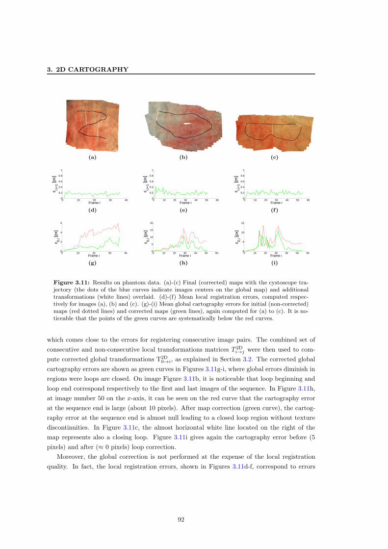
3. 2D CARTOGRAPHY
(a) (b) (c)
0 10 20 30 400
0.2
0.4
0.6
0.8
1
Frame i
ε i,i+
1 [px]
(d)
0 10 20 30 40 50 600
0.2
0.4
0.6
0.8
1
Frame i
ε i,i+
1 [px]
(e)
0 10 20 30 40 50 600
0.2
0.4
0.6
0.8
1
Frame i
ε i,i+
1 [px]
(f)
0 10 20 30 400
2
4
6
Frame i
ε 0,i [p
x]
(g)
0 10 20 30 40 50 600
5
10
15
20
Frame i
ε 0,i [p
x]
(h)
0 10 20 30 40 50 600
5
10
15
Frame i
ε 0,i [p
x]
(i)
Figure 3.11: Results on phantom data. (a)-(c) Final (corrected) maps with the cystoscope tra-jectory (the dots of the blue curves indicate images centers on the global map) and additionaltransformations (white lines) overlaid. (d)-(f) Mean local registration errors, computed respec-tively for images (a), (b) and (c). (g)-(i) Mean global cartography errors for initial (non-corrected)maps (red dotted lines) and corrected maps (green lines), again computed for (a) to (c). It is no-ticeable that the points of the green curves are systematically below the red curves.
which comes close to the errors for registering consecutive image pairs. The combined set of
consecutive and non-consecutive local transformations matrices T 2Di→j were then used to com-
pute corrected global transformations T2D0→i, as explained in Section 3.2. The corrected global
cartography errors are shown as green curves in Figures 3.11g-i, where global errors diminish in
regions were loops are closed. On image Figure 3.11b, it is noticeable that loop beginning and
loop end correspond respectively to the first and last images of the sequence. In Figure 3.11h,
at image number 50 on the x -axis, it can be seen on the red curve that the cartography error
at the sequence end is large (about 10 pixels). After map correction (green curve), the cartog-
raphy error at the sequence end is almost null leading to a closed loop region without texture
discontinuities. In Figure 3.11c, the almost horizontal white line located on the right of the
map represents also a closing loop. Figure 3.11i gives again the cartography error before (5
pixels) and after (≈ 0 pixels) loop correction.
Moreover, the global correction is not performed at the expense of the local registration
quality. In fact, the local registration errors, shown in Figures 3.11d-f, correspond to errors
92

3.5 Results
0 10 20 30 400
0.5
1
1.5
Frame i
ε i,i+
1[px]
(a)
0 10 20 30 400
5
10
15
Frame i
ε 0,i[p
x]
(b)
Figure 3.12: Comparison of the new method (green lines) with the sparse graph-cut method (reddotted lines) described in Chapter 2 and (WDBH+na). (a) Registration error comparison. (b)Global cartography error comparison. It is noticeable that both the registration and cartographyresults are more accurate for the algorithms presented in this chapter. Moreover, the registrationalgorithm performs similar for each image pair, demonstrating its robustness and invariance tothe perspective transformation parameters.
after global correction, but are almost similar to those before global correction. The “zigzag”
sequence (Figure 3.11a) does not contain loops, so the global cartography errors increases with
time even after global optimization, and cannot be null at the sequence end. However, due
to the two additional transformations (white lines in Figure 3.11a) that link the three almost
rectilinear cystoscope trajectory parts, these global errors are strongly diminished.
For all three sequences, the errors between overlapping regions are low, leading to visually
coherent panoramic maps of the phantom data.
To put the performances of the proposed registration methods in perspective, they could be
compared to the different existing methods for white light bladder image registration, namely
the mutual information based method (MLHMD+04, MLDB+08), the optical flow method of
Baker and Matthews (HMBD+10), and the sparse graph-cut method described in Section 2.5
and published in (WDBH+na). However, in (WDBH+na), it was shown on phantom data (see
also Figure 2.17) that the sparse graph-cut method is by far the most accurate in comparison
to the mutual information and Baker and Matthews methods, independent of the parameters
of the tested perspective transformations. In other words, the results of (WDBH+na) let us
reason that the methods of (MLHMD+04, MLDB+08, HMBD+10) will lead to even higher
global cartography errors. For this reason, the registration algorithm described in this chapter
is only compared to sparse graph-cuts.
Tests performed in Chapter 2 have shown that the registration accuracy of the sparse graph-
cut method is very high (errors of some few tenths of a pixel) and almost independent of the
parameter values of the underlying perspective transformation. It is noticeable on Figure 3.12a
that the registration errors of this method is now by far larger (between 0.5 and 1 pixel error).
The reason for this drop in performance of the method of (WDBH+na) lies in the fact that the
simulated transformations were stronger than those tested in (WDBH+na). In (WDBH+na),
not only the perspective transformation changes were by far smaller, but the parameters did
also not change strongly in a simultaneous way.
93

3. 2D CARTOGRAPHY
To compare the sparse graph-cut approach and the new method proposed in this chapter
we have computed the map of Figure 3.11a with both methods. To be able to compare both
algorithms, no map corrections with additional non-consecutive image pairs was used. As can
be seen in Figure 3.12a, the registration error of (WDBH+na) is roughly between twice and
thrice as large in comparison to the errors of the method proposed in this chapter. The other
important result of the new registration method is that the registration error remains constant
(independent of the perspective transformation), and the images are robustly superimposed,
even for stronger perspective changes. It is also noticeable on Figure 3.12b that, for the sparse
graph-cut approach, the varying local registration errors lead to much higher global cartography
errors (twice as high after 25-30 images) than those of the method proposed in this chapter.
It should be noted that it was still possible to detect additional overlapping image pairs for
the sequence in Figure 3.11a. However, registering these additional pairs using the method of
(WDBH+na) did not lead to satisfying results. The energy got stuck in poor local minima
due to the strong perspective transformations involved. For the other phantom (and patient)
sequences, even some consecutive image pairs failed to register correctly with the sparse graph-
cut method, while such failures were not observed with the method described in this chapter.
Even if the registration and cartography algorithms presented in this chapter are very ac-
curate and robust, the comparison with (WDBH+na) justifies the statements made initially.
Globally accumulated cartography errors must be kept as low as possible, in order to be able to
detect sections of overlap and correct these errors. As robustly detecting non-consecutive image
pairs is required to build visually coherent maps, we can conclude that projectively invariant
energy formulation is an important step towards accurate registration and global cartography.
This helps to keep accumulated errors low for accurate overlap detection, and allows to register
non-consecutive image pairs, which are related by much stronger perspective transformations.
Registration of such non-consecutive image pairs is impossible with state-of-the-art white light
registration algorithms proposed in (MLHMD+04, MLDB+08, HMBD+10) and with the sparse
graph-cut method (WDBH+na).
3.5.2 Qualitative Evaluation on Clinical Data
Having quantitatively justified the improvements of the proposed registration methods on simu-
lated phantom data in the previous section, this section will present results obtained on clinical
data. Six cystoscopic video-sequences acquired at the comprehensive cancer center of Nancy
(Institut de Cancerologie de Lorraine, ICL) were processed to assess the applicability of the
proposed methods on patient data. The purpose of the each individual algorithm step will be
briefly recapitulated and discussed using the results.
94

3.5 Results
(a) (b) (c)
Figure 3.13: Image pre-processing. (a) Original image, de-interlaced. (b) Cropped sub-image,where distortions can be neglected. Illumination gradients are visible. (c) Illumination correctedimage, as used for the registration data terms of Section 3.3.1 and the contrast-enhanced seamlocalization described in Section 3.4.1. Note that the image of c) has been normalized for viewing.The visible noise is also present in the image of b), but not as visible in the original image.
Video Pre-Processing
Pre-processing is necessary to prepare the original cystoscopic video-sequences for robust car-
tography. First, the videos, recorded with the PAL standard, have to be de-interlaced. Then, a
400× 400 pixel sub-image is extracted from each image, where image distortions are negligible
(HMBD+10). The last step consists of removing illumination differences due to vignetting and
non-orthogonal angle of the cystoscope towards the epithelium. This is achieved by subtract-
ing a bandpass-filtered image from the de-interlaced and cropped input image, similar to the
method proposed in (HMBD+10), which was described in Section 1.3.1. Figure 3.13 shows these
pre-processing steps, and the illumination corrected images (Figure 3.13c) are used as input
for both the registration data terms (see Section 3.3.1), as well as for the contrast-enhanced
seam detection method (Section 3.4.1). Finally, from the initial 25 images per second video, a
subset of images depending on the overall speed of the cystoscope movement is extracted. In
our experiments, we extracted every tenth image.
Registration of Consecutive Image Pairs
For consecutive image pairs, the percentage of overlap is quite large and the translation com-
ponents of the perspective transformation are usually the dominant parameters. For instance,
when every tenth image is extracted from the video-sequence, consecutive images have a typical
overlap of 85% or more of the image area. In order to minimize the computation time, different
parameter sets were used for consecutive image pairs on the one hand, and for non-consecutive
image pairs on the other hand. The parameters given in Table 3.2 (see Equation (3.8)) are used
for the registration of consecutive image pairs.
95

3. 2D CARTOGRAPHY
α β γ δ kmax r11 0 1 0 8 75 pixels
Table 3.2: Constant parameters used for consecutive image registration. These parameterscorrespond to those of Equation (3.8). Due to translation dominated perspective transformationslinking consecutive images (see also Figure 3.14), it is sufficient to use second-order data andfirst-order regularization terms. This leads to potential costs easier to minimize and consequentlyto faster convergence time, as opposed to the parameter set necessary for non-consecutive imagepairs (Table 3.3).
(a) (b)
(c) (d)
Figure 3.14: Examples of the registration of consecutive images pairs. The images usually sharea large percentage of overlap, and while the contrast of the images varies throughout the video-sequence, it is similar between successive images. In each sub-figure, from left to right: image Iitransformed to the coordinate system of Ij ; Ij ; estimated displacement vector field.
Constant parameters were used for all consecutive pairs, but were not exhaustively fine-
tuned. In turn, variations between 50 − 200% of the parameter γ (pairwise regularization of
Equation (3.6)) do not change the resulting displacement field noticeably, which emphasizes
the robustness of the second-order data terms. Figure 3.14 shows a few examples of registered
consecutive image pairs. The geometric relationship is dominated by translations, while rotation
and scale changes are also often observed, especially when the cystoscope’s direction changes.
As only second-order data terms and pairwise regularization terms are used for the regis-
tration of consecutive images, computation time is significantly lower than the time needed to
superimpose non-consecutive images. A pair of consecutive images is registered in ten to twenty
seconds1. While the BHS algorithm itself is difficult to parallelize2, the registration of different
1All experiments were computed on a quad-core 3.3GHz desktop computer with 16 GB of RAM, runningUbuntu 12.04.
2There are parallel graph-cut implementations available (e.g. (VN08)), but they are only suitable for regulargrids. Auxiliary variables induced by higher-order terms do not fit in this formulation, neither do irregular graphstructures.
96

3.5 Results
α β γ δ kmax r11 0 1 0 6 125 pixels
(a) Parameter set for k = 1
α β γ δ1 0 0 500
(b) Parameterset for k > 1
Table 3.3: Constant parameters used for non-consecutive image registration, corresponding toEquation (3.8). (a) At the coarsest pyramid level (k = 1), higher-order regularization may leadto a large number of non-submodular terms when the initial transformation deviates from thetrue transformation. To prevent poor local minima, pairwise regularization is used at the initialpyramid level. (b) Parameter set for the remaining levels (k > 1). Due to the large numberof non-submodular terms when using third-order data terms (Equation (3.5)) and fourth-orderregularization (Equation (3.7)), these two terms cannot be used simultaneously.
(a) (b)
(c) (d)
Figure 3.15: Examples of the registration of non-consecutive images pairs. Note the varyingcontrast between non-consecutive images (e.g. in a)) and the low percentage of overlap (b-d).These image pairs cannot be registered using state-of-the-art white light registration methods(MLHMD+04, MLDB+08, HMBD+10, WDBH+na). Using the proposed higher-order data andregularization terms, approximately invariant to projective transformations, allows to register suchimage pairs robustly.
image pairs can be easily distributed to several cores, as each CPU can process a pair of images
in parallel. When every tenth image is extracted from the video (as done in the experiments),
one second of a cystoscopic video can be processed in 7-14 seconds using four CPUs.
Registration of Non-Consecutive Image Pairs
Non-consecutive image pairs are registered using the constant parameters given in Table 3.3.
Some examples of registered non-consecutive images pairs are given in Figure 3.15. As can be
seen there, such image pairs may share a low percentage of overlap (e.g. Figures 3.15b-d), may
be related by strong variations in the displacement vector field, and often differ in contrast (see
97

3. 2D CARTOGRAPHY
Figure 3.15a).
Due to potential displacements of large magnitude and low overlap, the fully projective
third-order data term and the perspective-enforcing fourth-order regularization term seem to
be the best choice for accurate registration of non-consecutive image pairs. Unfortunately, using
both Equation (3.5) and Equation (3.7) (i.e. β > 0 and δ > 0) leads to a very low percentage of
labeled vertices due to the large number of non-submodular terms after reduction to pairwise
interactions. While roughly 40% of image pairs could be accurately registered, it was not
systematically possible (i.e. for the majority of non-consecutive image pairs, the solution got
trapped in poor local minima). However, the second-order data terms of Equation (3.4) lead
to a valid approximation of the perspective transformation model. For this reason, we have
discarded the fully perspective data terms in favour of the perspective-enforcing fourth-order
regularization terms, which are crucial for robustly registering non-consecutive image pairs.
It is noticeable that Equation (3.7) still leads to a significant number of non-submodular
terms at the initial level in the proposed coarse-to-fine minimization scheme. If the initial
transformation is inaccurate and deviates strongly from the transformation to be found at
the coarsest pyramid level, both Epq(xcp, x
cq) (i.e. initial solution) and Epq(x
pp, x
pq) (proposed
solutions) will have large costs1. These costs will violate the submodularity constraint of Equa-
tion (2.8) and lead to many vertices being unlabeled. In such cases, the solution obtained after
the coarsest level will be far from the true transformation to be found, and consequently, the
minimization will get trapped in poor local minima. In order to prevent wrong initial registra-
tion at the coarsest pyramid level, the parameters given in Table 3.3a are used at the initial
pyramid level. For the remaining levels, the parameters given in Table 3.3b are used. This
ensures that an initial solution close to the global minima is reached and enough variables can
be labeled when using Equations (3.4) and (3.7) in the remaining pyramid levels.
These terms lead to computation times significantly longer (30 - 60 seconds per pair and
CPU) than those for registering consecutive image pairs. However, the number of non-con-
secutive image pairs is much smaller than the set of consecutive pairs, so the increase of com-
putation time has less influence on the computation time of the entire sequence. For instance,
for the patient data of Figure 3.16, 75 images are linked by consecutive T2Di→i+1 matrices, while
only 6 non-consecutive image pairs were selected. The computation time of the 75 consecutive
images is about 1000 seconds, while the non-consecutive images are registered in 6 × 45 = 270
seconds. Such processing times are compatible with a second diagnosis and patient interview
shortly after the examination.
Global Map Correction
After all consecutive image pairs have been registered, the subset of additional overlapping im-
age pairs can be determined (i.e. the non-consecutive image pairs that have to be registered).
1After reduction of higher-order potentials to their equivalent pairwise form.
98

3.5 Results
12
34
56
I0I74
Misalignment
Figure 3.16: Determining a subset of overlapping, non-consecutive image pairs. The cystoscopetrajectory (grey lines) and the image centers (green dots) are overlaid on the initial (uncorrected)map. The accumulated cartography error is visible between first (I0) and last (I74) images of thesequence near the bottom left hand side, as indicated by the grey rectangle. The additional imagepairs are indicated by white lines, and the chronological order in which they have been determinedis indicated by the numbers. The corrected map can also be seen in Figure 3.18.
Figure 3.16 represents a map built only using consecutive transformations (i.e. no map cor-
rection was applied), and illustrates how and in which chronological order additional pairs are
found. The cystoscope trajectory (grey lines) is projected on the map, and the center of each
image is indicated with a green cross. The global cartography error is visible in the bottom
left part of the map (indicated by the grey rectangle) between first I0 and last I74 images
of the sequence, but low enough to be able to correctly detect additional overlapping image
pairs. These are indicated by white lines, and the corresponding number indicates in which
chronological order these pairs have been determined.
Whether the search for additional image pairs will be successful or not depends on the
amount of accumulated error during the cartography process. This error is often directly
connected to the number of images acquired before returning to a previously visited location.
Indeed, the more images are registered, the more the global errors accumulate. However, errors
also increase quickly when a few pairs of images are inaccurately registered. When accumulated
errors become too large, non-consecutive images that actually capture a common region on the
bladder surface might not overlap at all in the estimated initial global transformations. An
example for this situation is shown in Figure 3.17d. The cystoscope trajectory is overlaid
with black lines, and found additional image pairs are indicated by white lines. The map
is constructed using the optimized global transformations, so visible misalignments due to
accumulated errors are already removed. It is noticeable however that no additional pair was
found in the top left part of the map. This is due to the fact that in this video-sequence, the
images are degraded by tissue floating in front of the camera. This influences the registration
99

3. 2D CARTOGRAPHY
(a) (b) (c)
(d)
0 50 100 1500246
Frame #
DM
GM
(e)
Figure 3.17: Exposure correction and the effects of floating tissue degradation on image regis-tration accuracy and overlap detection. (a) Images placed into the global map coordinate systemusing the found seams. While all vascular structures are well aligned, exposure related artefactsare strongly noticeable. After exposure correction, the map in (d) shows visually coherent transi-tions. (b),(c) Consecutive image pair, degraded by floating bladder tissue. Such degradations leadto less accurate image registration when using first-order regularization. The thus accumulatederrors led to the top cystoscope trajectory being estimated further to the top in the intial map,and no additional pairs with enough overlap could be detected in the top left part of the mapcoordinate system. However, the errors were low enough to detect the four additional transfor-mation on the right hand side (after the 180 degree trajectory change). The perspective-invarianthigher-order regularization terms are robust against floating tissue, and the obtained shortcuttransformations significantly reduced accumulated errors. For this reason, the map could still bestitched seamlessly, and even in the top left hand side, all vascular structures are well aligned.
100

3.5 Results
accuracy, leading to larger local registration errors. An example for a consecutive image pair
where floating tissue complicates registration1 is shown in Figures 3.17b-c. Local errors in
this map region led to the top cystoscope trajectory improperly estimated further to the top.
Consequently, no overlap could be detected in that region. However, the error was still low
enough to detect the four additional pairs near the trajectory direction change (white lines
at the right side). As these corresponding non-consecutive image pairs were registered using
the perspective-invariant higher-order regularization term, the floating tissue did not have a
noticeably degrading influence on the local registration accuracy. Thus, the obtained “shortcut”
transformations led to much lower accumulated errors, and the map could be stitched seamlessly
(as can be seen in Figure 3.17d). Using these optimized transformation matrices, additional
overlapping image pairs could be detected in a second iteration of the algorithm.
For all experiments, the parameters of Algorithm 1 were set to tδ = 0.2 and tϑ = 0.7.
Map Compositing
After all consecutive and selected non-consecutive image pairs have been successfully registered,
and global map correction has been applied, the images can be placed into the common map
coordinate system to compose the final panoramic image. As stated earlier, small movements
of the bladder surface and small errors due to the non-flat surface of the organ will still lead to
small (but visible) misalignments of vascular structures, especially for overlapping cystoscope
trajectory parts. At the same time, cystoscope de-focus and motion blur vary throughout the
sequence. The goal of the contrast-enhancing seam correction method proposed in this chapter
is to correct these small misalignments, and select the sharpest images for each region of the
panoramic map. Figure 3.18 demonstrates the efficiency of the proposed method when using
different regularization weights. Higher regularization weight (λseam = 1 of Equation (3.10))
leads to relatively small seam lengths, as shown in Figures 3.18b&f. Small misalignments
are removed, but contrast enhancement is not optimal. Using a lower regularization weight
(Figures 3.18c&g) of λseam = 0.01 leads to both seamless alignment and visibly enhanced
contrast. For all cystoscopic video-sequences processed, the parameter λseam of Equation (3.10)
was set to 0.01 and led to visually coherent and contrasted maps.
In order to evaluate the advantages of the proposed compositing method, it is compared
with distance based feathering (see again Section 1.3.4), which was used in several contributions
to bladder cartography (WRS+05, HMBD+10, BGS+10)1. The major part of the images of
the cystoscopic sequence used to generate the panoramic map shown in Figure 3.19 consists of
blurry images, mostly due to cystoscope de-focus. One example of a very blurry image is shown
1It is recalled that for the registration of consecutive images, first-order regularization is employed to reducecomputation time. Perspective-invariant higher-order regularization do not suffer from floating tissue, and couldpotentially be used also for consecutive image pairs when floating tissue is detected.
1It is recalled that the method proposed in (BGS+10) uses feathering based on the intensity of the inputimages, as the fluorescence emitted by tumorous cells corresponds to high intensities decays rapidly. Nevertheless,contrast or structure misalignments are not considered there neither, so the results of this section also apply forintensity based feathering.
101
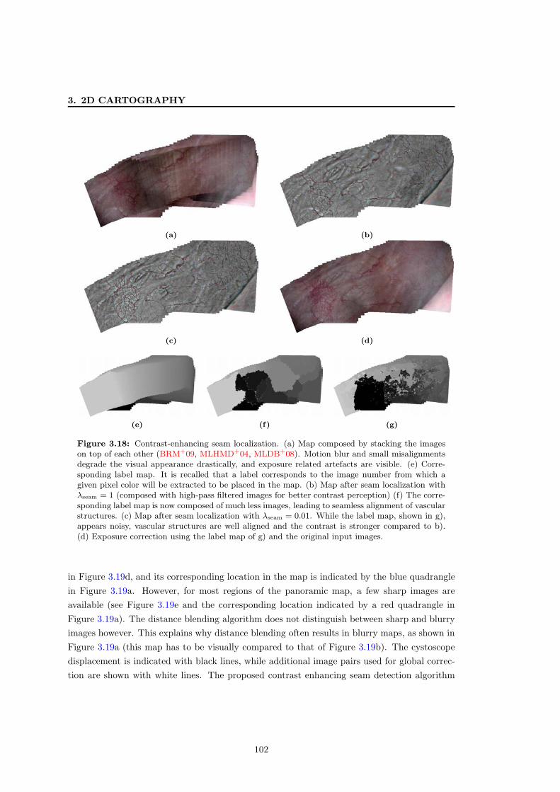
3. 2D CARTOGRAPHY
(a) (b)
(c) (d)
(e) (f) (g)
Figure 3.18: Contrast-enhancing seam localization. (a) Map composed by stacking the imageson top of each other (BRM+09, MLHMD+04, MLDB+08). Motion blur and small misalignmentsdegrade the visual appearance drastically, and exposure related artefacts are visible. (e) Corre-sponding label map. It is recalled that a label corresponds to the image number from which agiven pixel color will be extracted to be placed in the map. (b) Map after seam localization withλseam = 1 (composed with high-pass filtered images for better contrast perception) (f) The corre-sponding label map is now composed of much less images, leading to seamless alignment of vascularstructures. (c) Map after seam localization with λseam = 0.01. While the label map, shown in g),appears noisy, vascular structures are well aligned and the contrast is stronger compared to b).(d) Exposure correction using the label map of g) and the original input images.
in Figure 3.19d, and its corresponding location in the map is indicated by the blue quadrangle
in Figure 3.19a. However, for most regions of the panoramic map, a few sharp images are
available (see Figure 3.19e and the corresponding location indicated by a red quadrangle in
Figure 3.19a). The distance blending algorithm does not distinguish between sharp and blurry
images however. This explains why distance blending often results in blurry maps, as shown in
Figure 3.19a (this map has to be visually compared to that of Figure 3.19b). The cystoscope
displacement is indicated with black lines, while additional image pairs used for global correc-
tion are shown with white lines. The proposed contrast enhancing seam detection algorithm
102
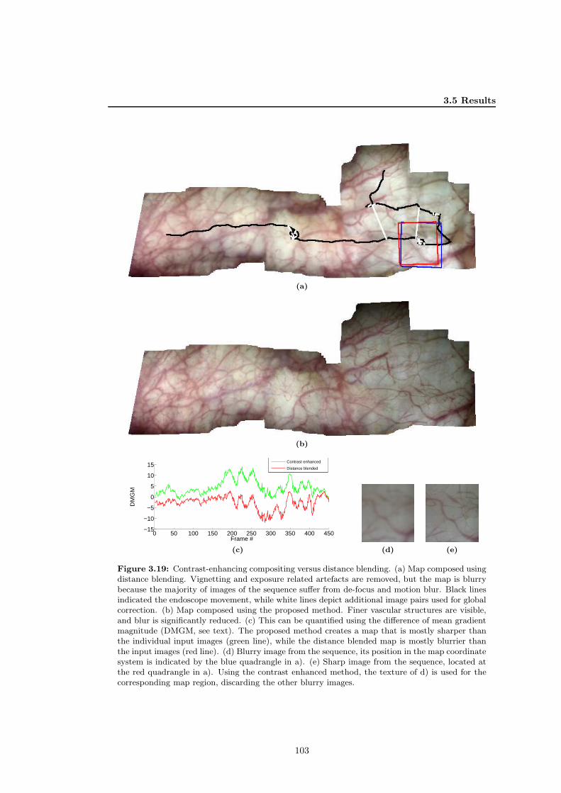
3.5 Results
(a)
(b)
0 50 100 150 200 250 300 350 400 450−15
−10
−5
0
5
10
15
Frame #
DM
GM
Contrast enhanced
Distance blended
(c) (d) (e)
Figure 3.19: Contrast-enhancing compositing versus distance blending. (a) Map composed usingdistance blending. Vignetting and exposure related artefacts are removed, but the map is blurrybecause the majority of images of the sequence suffer from de-focus and motion blur. Black linesindicated the endoscope movement, while white lines depict additional image pairs used for globalcorrection. (b) Map composed using the proposed method. Finer vascular structures are visible,and blur is significantly reduced. (c) This can be quantified using the difference of mean gradientmagnitude (DMGM, see text). The proposed method creates a map that is mostly sharper thanthe individual input images (green line), while the distance blended map is mostly blurrier thanthe input images (red line). (d) Blurry image from the sequence, its position in the map coordinatesystem is indicated by the blue quadrangle in a). (e) Sharp image from the sequence, located atthe red quadrangle in a). Using the contrast enhanced method, the texture of d) is used for thecorresponding map region, discarding the other blurry images.
103

3. 2D CARTOGRAPHY
on the other hand stitches the panoramic map using as much contrast as possible without mis-
aligning vascular structures. The result, shown in Figure 3.19b, shows even very fine vascular
structures and is overall more contrasted than the map of Figure 3.19a. This observation can
also be quantified using a simple measurement, which we refer to as difference of mean gradi-
ent magnitude (DMGM). It is computed by subtracting the mean gradient magnitude of each
input image from the mean gradient magnitude of the corresponding region in the map. The
green curve of Figure 3.19c shows that this difference is positive for almost all images of the
sequence when computed for the map shown in Figure 3.19b. In other words, the contrast of
most images’ regions in the map is stronger than for the corresponding images themselves. For
instance, the peak at image number 250 in Figure 3.19c corresponds to the image shown in
Figure 3.19d. As this image is very blurry, the contrast enhancement in the map is high. If an
input image is well contrasted, the enhancement is very low (i.e. the valley at image number
272 corresponds to a DMGM of ≈ 0), which means that this image contributed strongly to the
final map. The DMGM for the distance blended map (red curve in Figure 3.19c) on the other
hand is mostly below 0, indicating the visual degradation induced by simple blending without
considering the images’ quality.
When optimal seam positions have been determined, illumination and color differences
across seams need to be removed. The parameter for the proposed exposure correction meth-
ods was set to λexp = 1 (see Equation (3.14)), and lead to satisfying results for all sequences.
Figure 3.17a shows the map before exposure correction, where the different exposure of the indi-
vidual input images is clearly visible. After exposure correction, the map shown in Figure 3.17d
is visually coherent (i.e. no visible exposure artefacts can be seen), while retaining the contrast
obtained after seam detection. This is backed by the DMGM, plotted in Figure 3.17e. The
green curve is again mostly positive, confirming that the map maximizes the contrast available
in the redundant data of the sequence.
Additional Map Examples
In Figure 3.20a, the ureter opening is visible and can act as an anatomical landmark. When
the map is archived and used later (some weeks or months after the examination) by another
urologist, maps with such landmarks can facilitate navigation towards regions of interests.
The map of Figure 3.20b includes a lesion. Showing lesions in a large field of view facilitates
diagnosis and follow up (lesion evolution assessment) by comparing maps computed at a given
time interval. It is visible on both figures that the maps are visually coherent (i.e. no texture
or color discontinuities are visible). Moreover, the the maps are well contrasted in every region
and without blur.
104

3.5 Results
Ureter opening
(a)
Lesions
(b)
Figure 3.20: Contrast-enhanced panoramic images for two additional cystoscopic video-sequences. (a) The ureter opening in visible. Such an anatomical landmark facilitates navigationduring a cystoscopy, and mental orientation weeks or months after the examination when prepar-ing for follow-up. (b) Map showing lesions. This large FOV image can be used to assess lesionevolution over time, either by comparing with another map, or during the cystoscopy itself.
105

3. 2D CARTOGRAPHY
3.5.3 Results on Traditional Applications
While the methods developed and proposed in this chapter were specifically tailored to create
large FOV maps from cystoscopic image sequences, they are also usable in more general appli-
cations. This section will show two examples, namely a set of images of a tourist attraction
stitched seamlessly, and high dynamic range images composed from partly overlapping images
with very different exposure levels.
Consumer Photography Stitching
An example for tourist stitching using the methods proposed in this chapter is shown in Fig-
ure 3.21, which has been composed from a sequence of 16 partly overlapping images. Consec-
utive images overlap by ≈ 50%. While this is much less than in a cystoscopic video-sequence,
the images contain sufficient image primitives. Both consecutive and non-consecutive image
pairs could consequently be robustly registered. However, as the large FOV leads to strongly
distorted transformed images (see again Figure 1.9 in Chapter 1), the images were transformed
to spherical coordinates after registration in order to produce a better scaled panoramic image.
While the result may not impress at first glance (and in fact, when watching semi-closely,
misalignments can be observed), stitching the transformed input images seamlessly is not trivial.
The registration of both consecutive and non-consecutive images leads to visually coherent
image superimposition, as shown in Figures 3.22a-b. However, the spherical projection model
induces bending of straight lines in the peripheral image regions, and as the images overlap
only by about 50%, this leads to oppositional bending in the overlapping image regions, as
shown in Figures 3.22c-d. Consequently, finding seams that align all images without visible
discontinuities is much more difficult when using spherical coordinates and sparsely overlapping
images. However, it is visible in Figure 3.21 that these seams were found and led to a visually
coherent panoramic image, especially when compared to the initial map, as shown in the top
left hand side of Figure 3.21.
High-Dynamic Range Images
The methods proposed in this chapter may also be used to create high-dynamic range (HDR)
images. An example is shown in Figure 3.23. HDR imaging aims at creating higher dynamic
range than a camera is able to capture from a single exposure level. In a single image, loss of
detail in dark (Figure 3.23a) or bright (Figure 3.23b) regions is evident. An HDR algorithm
allows to reduce such loss of detail by combining multiple images taken with different exposure
levels. The resulting image should be well exposed in both dark and bright image regions. The
methods proposed in this chapter are also capable of producing HDR images. The two input
images of Figures 3.23a-b were taken with a hand-held smartphone camera, and registered using
106
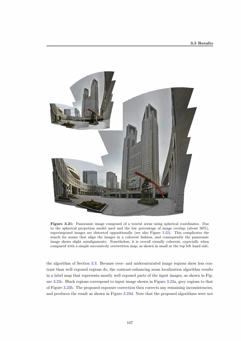
3.5 Results
Figure 3.21: Panoramic image composed of a tourist scene using spherical coordinates. Dueto the spherical projection model used and the low percentage of image overlap (about 50%),superimposed images are distorted oppositionally (see also Figure 3.22). This complicates thesearch for seams that align the images in a coherent fashion, and consequently the panoramicimage shows slight misalignments. Nonetheless, it is overall visually coherent, expecially whencompared with a simple successively overwritten map, as shown in small at the top left hand side.
the algorithm of Section 3.3. Because over- and undersaturated image regions show less con-
trast than well exposed regions do, the contrast-enhancing seam localization algorithm results
in a label map that represents mostly well exposed parts of the input images, as shown in Fig-
ure 3.23c. Black regions correspond to input image shown in Figure 3.23a, grey regions to that
of Figure 3.23b. The proposed exposure correction then corrects any remaining inconsistencies,
and produces the result as shown in Figure 3.23d. Note that the proposed algorithms were not
107

3. 2D CARTOGRAPHY
(a) (b)
(c) (d)
Figure 3.22: Image misalignment due to spherical warping. (a) Image Ii, transformed into thecoordinate system of image Ii+1. (b) Image Ii+1. The images are adequately aligned. (c)-(d) Likea) and b), but using a spherical projection model. (c) A green cross denotes the position of avertex after transformation into spherical coordinates. (d) A green cross shows the correspond-ing position (again, in spherical coordinates), as estimated by the registration algorithm. Theestimated correspondences still correspond to homologous positions, but the spherical projectionviolates the assumption of a perspective transformation. This is illustrated by a blue cross in d),which corresponds to a green cross in c), transformed using T2D
i→i+1.
designed to produce HDR images, and consequently, we did not perform a comparison with
state-of-the-art techniques. It is however straightforward to integrate data and regularization
terms better suited for HDR imaging.
108

3.6 Discussion and Perspectives
(a) (b)
(c) (d)
Figure 3.23: High-dynamic range image composition. (a) First input image, captured with shortexposure time. (b) Second input image, captured with long exposure time. (d) Composed high-dynamic range image. As over- and under-saturated image regions have a lower contrast than wellexposure regions, the contrast-enhanced seam localisation algorithm is able to assign each pixel acorresponding, well-exposed image index, as shown in c). After exposure correction, the dynamicrange of the image is much larger than for each individual input image.
3.6 Discussion and Perspectives
3.6.1 Practical and Scientific Contributions
The methods proposed in this chapter allow to construct real large field of view panoramic
images from cystoscopic video-sequence. The term “real” stands in opposition to those al-
gorithms which are only able to construct band-shaped maps with a large FOV in one main
direction without visible accumulated errors. Indeed, previous contributions did not consider
the problem of accumulated errors, and presented registration algorithms that are not suitable
109

3. 2D CARTOGRAPHY
to systematically register non-consecutive image pairs. Consequently, only strip-shape maps
(such as the one shown in Figure 1.5) constructed from consecutive image transformations were
presented before. An exception is the method proposed in (BTGA11), where gaps in the map
are detected using a frame-graph structure. This is potentially useful for clinicians, as they can
immediately assess whether they have missed to scan parts of the epithelium. However, this
method does not consider accumulated errors neither, and only results on phantom data are
given, where error accumulation is significantly lower.
In the following, we will summarize the main contributions of this chapter.
Automatic Detection of Cystoscopic Trajectory Crossings and Correction of Globally Accu-
mulated Cartography Errors
Accumulated cartography errors have to be corrected for crossing endoscope trajectories and
for loop scenarios. Image registration is generally computationally intensive for the white light
modality because image primitives cannot be systematically extracted, which makes iconic data
registration necessary. Due to time constraints, registering all possible consecutive and non-
consecutive image pairs is infeasible. Therefore, in order to correct accumulated errors, we
use a specific graph structure that represents the images and their relationship in the global
coordinate system. This allows to automatically select a meaningful subset of overlapping non-
consecutive images, and the transformations relating these pairs are used to correct accumulated
errors using sparse non-linear least squares.
Invariant Energy Functions for Image Registration
Non-consecutive image pairs are often linked by image displacements of large magnitude and
small image overlap. To deal with this we have proposed data and regularization terms which
compute energy costs invariantly to the perspective transformation parameter values that link
overlapping images. This is possible using higher-order interaction between pixels, which are
reduced to an equivalent pairwise form using reduction by minimum selection. In addition,
a coarse-to-fine minimization scheme which significantly reduces the computation time com-
pared to classical iterative minimization methods was proposed. Both consecutive as well as
non-consecutive image pairs for six clinical datasets could systematically be registered. The
registration was performed using constant parameter sets (a separate set for consecutive and
non-consecutive image pairs), which demonstrates the robustness of the proposed method. This
robustness is important for potential clinical use, as clinicians should not have to adjust algo-
rithm parameters in order to obtain usable maps.
Contrast-Enhancing Map Compositing
Unlike previous contributions, which use blending techniques to compose the textured panoramic
image, we have proposed an energy minimization based seam detection algorithm. This method
allows to correct small misalignments of vascular structures when stitching the map. At the
same time, it maximizes the map’s quality by favouring contrasted images over blurry ones. In
110

3.6 Discussion and Perspectives
a second step, exposure related artefacts are removed without interpolation across seams, while
contrast and hue of the original input images are retained. The thus constructed panoramic
images are generally of better or equal quality than the individual input images. This allows
clinicians to see the scanned parts of the epithelium in a single high-resolution image.
3.6.2 Limits of the Methods and Perspectives
While all of the proposed methods have theoretical limits, the global and practical limit of the
cartography process is the accumulation of local registration errors to global cartography errors.
Even with the proposed registration method, which systematically (i.e. robustly) registers con-
secutive images with high accuracy, errors still accumulate. Even if both perspective-invariant
data and regularization terms cannot be used jointly due to the large number of non-submodular
terms, the accuracy of registering non-consecutive image pairs is still acceptably close to that
of consecutive registration. So as long as accumulated errors are low enough to detect valid
additional non-consecutive image pairs, the proposed registration algorithm is able to superim-
pose these images with satisfying accuracy. Possibly, the order reduction method proposed in
(GBP11) might be able to obtain less non-submodular pairwise terms, so that both perspective-
invariant data and regularization terms can be used jointly.
However, as was shown in Figure 3.17, when overlapping parts of the map cannot be detected
because accumulated errors are too large, the corresponding map regions cannot be accurately
corrected. As previously discussed, it was still possible to correct the accumulated errors with
the help of two additional transformations and the higher-order potential functions, but this
cannot always be guaranteed. An obvious solution is a semi-automatic implementation, where
missed trajectory overlaps can be manually selected by the clinician. Exhaustive search of
overlapping map regions is also a possibility. This will, however, increase computation time
significantly, and it is not straightforward to reject image pairs that do not overlap. In other
words, the question whether two images show homologous bladder texture remains an open
problem, as all iconic based image registration techniques (existing state-of-the-art methods, as
well as those presented in this chapter) will return a local transformation matrix.
Another practical limit is the distortion observed when the FOV is large due to the per-
spective transformation model used. For instance, in Figure 3.17d, the size of the first image
of the sequence (bottom most image) is much smaller than the last image of the sequence.
Similar observations can be made in relevant publications concerning bladder cartography. A
spherical projection model would be ideal, but without knowledge of the cystoscope position
and orientation relative to the surface, the obtained cystoscope path will be incorrect and pre-
vent accurate detection of overlapping trajectories. As we shall see in the next chapter, with
such knowledge, it is possible to construct panoramic surfaces with accurate geometry, inde-
pendently of the field of view. Without such knowledge, a possibility is to allow the clinicians
to select an appropriate reference image on the fly. This will minimize perspective distortions
111

3. 2D CARTOGRAPHY
in regions around the point of interest. However, when a change of reference coordinate system
infers a strong change in local panoramic resolution, the map compositing process must be
re-computed, adding additional computation time.
Finally, the greatest potential in reducing the computation time of the cartography process
lies in image registration. The methods proposed in this chapter represent an approach focused
on both robustness and accuracy, and outperform state-of-the-art algorithms in these terms.
This registration quality comes with the disadvantage of longer computation times, compared
for instance with feature based approaches. These can potentially be used in real-time, but
cannot guarantee robust registration for the entire video-sequence. Future research should be
targeted at selecting an appropriate registration algorithm based on the texture quality of the
input images Ii and Ij . Indeed, many consecutive image pairs can be accurately registered
with faster algorithms, such as feature based approaches, sparse graph-cuts, or fast optical flow
algorithms. If an image texture analysis algorithm can robustly predict the probability of a
successful registration for a given algorithm, the computation time can be significantly reduced
by choosing the fastest applicable algorithm. Furthermore, a Kalman filter can be used to
predict the cystoscope displacement T2Di→i+1 based on the previous registration result T2D
i−1→i.
This could allow to select the number of images that can be skipped without jeopardizing a
successful registration, potentially leading to a much smaller number of consecutive images to
be registered.
3.6.3 Publications
International Journal
• T. Weibel, C. Daul, D. Wolf, R. Rosch, and F. Guillemin. Graph based construction of
textured large field of view mosaics for bladder cancer diagnosis. Pattern Recognition,
45(12):4138 – 4150, 2012
International Conferences
• T. Weibel, C. Daul, D. Wolf, and R. Rosch. Planarity-enforcing higher-order graph cut. In
18th IEEE International Conference on Image Processing (ICIP), pages 41–44, September
2011. Brussels, Belgium (Oral presentation)
• T. Weibel, C. Daul, D. Wolf, R. Rosch, et al. Contrast-enhancing seam detection and
blending using graph cuts. In 21st International Conference on Pattern Recognition
(ICPR), pages 2732–2735, November 2012. Tsukuba, Japan (Oral presentation)
National Conference
• T. Weibel, C. Daul, D. Wolf, and R. Rosch. Customizing graph cuts for image registration
problems. In XXIIIe Colloque GRETSI Traitement du Signal & des Images (GRETSI),
September 2011. Bordeaux, France (Oral presentation)
112

Chapter 4
3D Cartography: a Proof of Concept
4.1 Introduction and Chapter Overview
In the previous chapter, it was shown how two-dimensional textured maps of the epithelium can
be built from cystoscopic video-sequences. The cartography process was divided into several
steps and processed sequentially. First, consecutive image pairs (Ii, Ii+1) were registered, and
the estimated local transformations T2Di→i+1 gave an initial estimate of the global transformations
T2D0→i. In the next step, accumulated cartography errors were automatically corrected. This
step required the development of a robust registration algorithm for non-consecutive image
pairs, which state-of-the-art algorithms are unable to register robustly. In the last step, small
remaining texture misalignments and exposure differences were corrected while simultaneously
maximizing the contrast of the map. The purpose of this chapter is to demonstrate that the
proposed two-dimensional cartography steps can be modified to build three-dimensional maps
(textured surfaces) when additional three-dimensional information is available.
However, while in Chapter 3 it was shown that the 2D cartography algorithm is applicable
on patient data, the work described in this chapter is limited to a proof of concept. Indeed,
phantom data, provided by prototypes simulating the acquisition principle of potential 3D-
endoscopes, are used as a first validation of the proposed 3D cartography method. Section 4.1.1
will first recapitulate the advantages of such three-dimensional textured surfaces over two-
dimensional maps for clinical diagnosis. Then, Section 4.1.2 presents the particular choice of
3D cartography principle used in this chapter. More details on previous contributions to 3D
endoscopic cartography were given in Section 1.4.
Available acquisition prototypes are described in Section 4.2. In essence, these prototypes
can be used to obtain additional three-dimensional information for each acquired color image.
This additional data allows for modifying the 2D cartography approach of the previous chapter.
It is important to stress that these prototypes are not yet applicable in clinical examinations.
Consequently, no clinical data sets are available. Nonetheless, the results on realistic phantom
113

4. 3D CARTOGRAPHY: A PROOF OF CONCEPT
data demonstrate the potential of the proposed algorithms to three-dimensional cartography.
Moreover, to highlight the flexibility (interest of the method for non-medical scenes), the al-
gorithm was not only applied to bladder phantoms. To do so, the algorithm was used for the
cartography of indoor datasets acquired with a Microsoft Kinect sensor, which is described in
Section 4.2.3.
Section 4.3 will outline the steps of the three-dimensional cartography algorithm (which are
individually described from Sections 4.3.2 to 4.3.4), with a focus on the differences between two-
and three-dimensional cartography. The proposed algorithms are tested on several data sets in
Section 4.4. The chapter concludes with a discussion and potential perspectives in Section 4.5.
4.1.1 Motivation and Projection Geometry
Clinicians try to mentally visualize the bladder’s three-dimensional structure while they scan
the epithelium for potential lesions. In other words, when clinicians observe the video-sequence,
each currently observed FOV (two-dimensional projection in form of the image Ii) is intuitively
perceived at (or re-projected onto) its corresponding location on the surface of the epithelium.
The aim of a three-dimensional cartography algorithm is to automatically carry out this re-
projection, i.e. to reconstruct the three-dimensional texture representation of the observed
bladder surface from a video-sequence.
Technically, each observed small FOV is a two-dimensional projection of a part of the organ’s
internal wall onto the plane of image Ii (see Figure 4.1). Let P3Di be a finite (sub-)set of three-
dimensional points on the epithelium, expressed in the (local) coordinate system of acquisition i.
As before, a subscript i = 0 indicates the global and common reference 3D coordinate system of
the map. A video-sequence consists of N acquistions, with i ∈ {0, ..., N−1}. The homogeneous
coordinates of a point p3Di,k ∈ P3Di with index k, expressed in the coordinate system of viewpoint
i, are defined by [Xi,k Yi,k Zi,k 1]T. This point is transformed into the local coordinate system
of acquisition number j by the rigid transformation T3Di→j , whose 3D rotation matrix R3D
i→j and
translation vector t3Di→j are defined in Equation (1.3):
p3Dj,k′ = T3Di→j p3Di,k =
[R3D
i→j t3Di→j~0 1
]
i→j
p3Di,k . (4.1)
In the remaining parts of this chapter, indices k and k′ represent homologous points displaced
from the coordinate system of acquisition i into that of acquisition j. We will also use the
notation T3Di→j(P
3Di ), which transforms all p3Di,k ∈ P3D
i to the coordinate system of viewpoint
j using Equation (4.1). The corresponding two-dimensional homogeneous projection p2Dj,k′ =
[xj,k′ yj,k′ 1]T ∈ P2D
j in the coordinate system of image Ij is then obtained by
p2Dj,k′ = νk
[
K~0] (
T3Di→j p3Di,k
). (4.2)
114

4.1 Introduction and Chapter Overview
bb
b
b
b
b
b
b
b
I0
Ii
Ij
KKT3D
0→i
KT3D0→j = KT3D
i→jT3D0→i
p3D0,k = T3D
i→0p3Di,k′
p2Di,k′
p2D0,k
T3D0→i
T3Di→j
T2D0→i
T2Di→j
C0
Ci
Cj
~yi~xi
~Yi
~Xi
~Zi
bb
b
b
b
b
Figure 4.1: Illustration of the image projection geometry. The rigid transformation T3Di→j relates
the coordinate systems of two acquisitions i and j. Points P3Di on the epithelium, expressed in
the coordinate system of acquisition i, are projected onto the image plane of acquisition j viaKT3D
i→j . When global transformations T3D0→i are known for each acquisition i, the surface can be
constructed by placing all P3Di into the coordinate system of the reference acquisition i = 0. C0,
Ci, and Cj correspond to the location of the camera’s optical centers in global coordinate system,and define the (local) 3D coordinate system origin for viewpoints 0, i and j, respectively. Thelocal 2D and 3D coordinate systems are illustrated for viewpoint 0, which also correspond to theglobal coordinate systems.
where P2Dj is a set of valid projections in the coordinate system of image Ij , K is the intrinsic
camera parameter matrix defined in Equation (1.1)1. The normalizing factor νk ensures that
the third element of p2Dj,k′ is equal to 1. The color vector at a (sub-pixel) position Ii(p2Di,k ) is
extracted from Ii using bilinear interpolation. If there exists a three-dimensional measurement
in acquisition i that can be associated with a pixel p, it will be addressed by p3Di,p for simplicity.
As in two-dimensions, the global transformation T3D0→i relating the local coordinate system
of acquisition i with the common global coordinate system (without loss of generality, assumed
to be identical with the first acquisition i = 0) is obtained via concatenation:
T3D0→i =
i−1∏
k=0
T3Dk→k+1. (4.3)
When 3D points P3Di and global transformations T3D
0→i are known for each acquisition i,
three-dimensional textured surfaces can be constructed. The advantages of such 3D maps are
manifold:1The images are assumed to be distortion-corrected beforehand.
115

4. 3D CARTOGRAPHY: A PROOF OF CONCEPT
• In comparison to two-dimensional maps, textured surfaces correspond more naturally
to the clinicians’ mental representation of the organ. Such a 3D representation should
therefore facilitate diagnosis and follow-up preparations.
• Two-dimensional maps are prone to strong perspective “deformations” between images ac-
quired with large instrument displacements and viewpoint changes (see Figure 1.9 and the
cartography results of the previous chapter). Therefore, map resolution varies with time
and cystoscope trajectory, but not necessarily with respect to the scale of the observed
bladder surface. Three-dimensional maps do not exhibit these degradations, as T 3D0→i is a
rigid transformation that preserves scale and shape of the observed scene. Accumulated
errors may still lead to inaccurate rigid displacements when returning to previously visited
locations, but do not affect either scale or shape of each viewpoint’s observed surface.
• A second “virtual” examination can be performed on the computer, allowing the clinicians
to navigate freely inside the textured three-dimensional map.
In the next section, we will briefly recapitulate existing approaches towards three-dimensional
cartography of endoscopic data and motivate the particular choice of reconstruction principle
used in this chapter.
4.1.2 Choice of 3D Map Reconstruction Principle
As discussed in Section 1.4, there are several potential approaches for constructing three-
dimensional surfaces from endoscopic video-sequences. Due to the quasi-planar surface part
observed in each small FOV, three-dimensional structure can only be recovered with the aid
of a priori information, or by using modified endoscopes. Indeed, as discussed in Section 1.4.3,
quasi-planar surfaces represent poor geometrical information (depth variations), which im-
pedes direct 3D-3D point registration algorithms, such as iterative closest points approaches
(BM92, Zha94, SHT09).
Moreover, the works described in Sections 1.4.1 and 1.4.2 show that neither 2D images
combined with a priori knowledge about the organ’s surface (CS09), nor SfM methods (SPS12)
are suitable for 3D bladder cartography.
As will be explained in the next section, additional three-dimensional data can be obtained
with devices that capture (sparse or dense) three-dimensional point sets P3Di for each viewpoint
i. Since the quasi-planar FOVs of cystoscopic images impede a direct 3D-3D data registration
due to a lack of geometrical surface information, the only solution is to use simultaneously the 2D
image texture and 3D point information to compute 3D maps. Such a strategy was successfully
applied in (BHDS+10), where the 3D surface construction was guided by 2D image registration,
and geometrical constraints allowed to converge towards the rigid 3D transformation effectively
linking two consecutive viewpoints i and i + 1 of a cystoscope prototype.
116

4.2 Data Acquisition
Two recent contributions (SFS+12, ANKB13) used additional external navigation systems
to facilitate the cystoscope position determination for each acquisition. The rigid cystoscope
displacement is estimated by tracking markers located on the external part of the cystoscope
with a stereo-camera system. Such a system allows to compute the cystoscope’s viewpoint in a
global coordinate system, relative to the stereo camera coordinate system (i.e. the coordinate
system is located in the examination room, not in the bladder). The approach proposed in
(SFS+12) also reconstructs the surface seen in each FOV using an active stereo-vision endo-
scope. Similar to (CLZQ03, BHSD+10), a set of 49 projected laser points is reconstructed in
each acquisition’s local coordinate system. These three-dimensional measurements are then
transformed into a common coordinate system via the estimated rigid cystoscope displacement.
The patient must remain still during the entire examination, as the rigid cystoscope displace-
ment is only measured via external tracking. Furthermore, no means of applying the texture
onto the reconstructed point cloud is proposed (no texture images were acquired). The ob-
jective of the approach proposed in (ANKB13) is merely to document the position of lesions
in order to quickly navigate to this position in a follow-up examination. As the bladder’s
three-dimensional structure is not reconstructed (i.e. no cartography algorithm is proposed),
clinicians do not benefit from extended FOV (showing lesions and anatomical landmarks), which
does not facilitate diagnosis. Both approaches require special equipment (including an external
tracking system present in the examination room), which infers additional costs and technical
problems. Moreover, as shown in (BHDS+10), 3D maps can be build without such additional
navigation systems.
We can conclude with the observation that robust three-dimensional cartography of cysto-
scopic video-sequences is feasible with a combination of two-dimensional image and additional
three-dimensional data (points on the bladder surface). External navigation systems (as used
in (SFS+12, ANKB13)) may facilitate the estimation of local rigid cystoscope displacements,
but are not sufficient alone to robustly compute global displacements in the organ’s coordinate
system. The methods developed in the remainder of this chapter therefore assume that modi-
fied cystoscopes allow to simultaneously capture color images Ii and a set of three-dimensional
measurements P3Di of the observed scene for each acquisition i. The advantage is that such
cystoscopes can be constructed using existing hardware (i.e. by modifying one- or two-channel
endoscopes). The next section will describe the available data of such modified cystoscopes and
present existing prototypes developed at the CRAN laboratory.
4.2 Data Acquisition
The prototypes available at the CRAN laboratory allow to capture a color image Ii (distortion-
corrected) and a set of (local) three-dimensional points P3Di on the surface in view. The following
subsection presents these prototypes in detail.
117

4. 3D CARTOGRAPHY: A PROOF OF CONCEPT
4.2.1 Laser-Based Cystoscope Prototype
An endoscope typically consists of two channels, while cystoscopes are one-channel systems. For
cystoscopes (and some two-channel endoscopes), the light source illuminates the observed scene
through a bundle of optical fibers, and the acquisition channel captures the reflected light using a
camera connected to the instrument. In (CLZQ03), the first channel of a two-channel endoscope
was used to project a dense laser dot matrix onto the observed surface, while the second channel
was used for image acquisition. The dot matrix was created by a collimated laser beam falling
on a diffractive optics. After accurate camera and dot matrix projector calibration, the three-
dimensional positions P3Di , corresponding to the dots P2D
i of the matrix, can be calculated in
the color camera coordinate system. The sub-millimeter reconstruction accuracy is remarkable,
given the small baseline of about 2.2 millimeters (the baseline corresponds to the distance
between the optical centers of camera and projector). However, as argued in Chapter 1, due to
the planar appearance in each image, robust 3D-3D registration using only P3Di and P3D
j is not
possible due to poor depth variations on the bladder surface. Even if T3Di→j could be estimated
robustly, the valuable texture information needed in the context of cytoscopy is lost due to the
dense dot-matrix projection.
To robustly reconstruct the observed surface together with the bladder texture, the method
proposed in (BHDS+10) uses eight projected laser points. By projecting only eight points
(ideally near the peripheral regions of the circular FOV of the cystoscope), the major part of
the texture is preserved, and visual inconveniences are minimized. The authors also proposed
a flexible camera-projector calibration technique (BHSD+10) that does not require expensive
calibration equipment. The method proposed in (BHSD+10, BHDS+10) can potentially by
implemented on one channel endoscopes (e.g. cystoscopes), and this one-channel solution can
be briefly described as follows.
The prototype (see Figure 4.2a) consists of a cylindrical tube, through which a cystoscope
is inserted. In addition, a green laser beam passes inside the tube and falls onto a diffractive
optics, located at the instrument distal tip (the laser beam is currently guided by mirrors
inside the cylindrical tube). This diffractive optics projects eight beams onto the surface. An
image acquired with this prototype is shown in Figure 4.2b. As illustrated in Figure 4.2d, a
triangulation technique can be used to compute the 3D coordinates of the laser dot centers
(BHSD+10). Tests with the prototype of figure Figure 4.2a have shown that the error on
the z coordinate is always smaller than a millimeter for a distance measure lying between 20
and 40 mm. This reconstruction is accurate for a baseline of 3 mm, and is sufficient when
3D shapes have to recovered (as in cystoscopy) without the aim to perform exact dimensional
measurements. The reconstructed points corresponding to the laser dots of Figure 4.2b are
shown in Figure 4.2c. Even if this prototype cannot be used directly in clinical conditions, its
geometry and scale (very small baseline of 3mm) is close to that of a cystoscope, and can be
potentially built by manufacturers.
118

4.2 Data Acquisition
Laser
CCD camera
Cylindrical tube
(cystoscope + guided laser beam)
Diffractive optic
Cystoscope distal tip
Baseline ≈ 3 mm
(a)
(b)
−10
10 −10 10
30
50
z[m
m]
y [mm]
x [mm]
(c)
p3Di,k
p2Di,k
Diffractive optic
Laser sourceLocal coordinate system i
(d)
Figure 4.2: Active stereo-vision principle of the laser cystoscope prototype. (a) Instrumentationprototype. (b) A set of eight laser rays is projected onto the color image. This allows to simulta-neously capture most of the bladder’s texture and (c) a set of eight three-dimensional positions,reconstructed in the camera coordinate system. (d) Geometry of this acquisition system. Onlyone of the eight diffracted laser beams is illustrated.
4.2.2 Time-of-Flight Prototype
The advantage of the method of (BHDS+10) compared to (CLZQ03) is that texture information
is not lost, but implies the disadvantage that only a very sparse set P3Di is available for each
acquisition. As shown in Section 4.4, dense point clouds acquired for each acquisition can
facilitate the 3D map construction in comparison to sparse 3D data per viewpoint. On the other
hand, the solution of (CLZQ03) was designed for two-channel endoscopes and is not applicable
with one-channel cystoscopes (a second channel is required for the pattern projection). For the
prototype of Figure 4.2, the diffractive optics is placed at the output of the cylindrical tube,
and an optical fiber can illuminate this optics with a laser light, avoiding the need of a second
channel. However, only manufacturers can decide if such a solution is feasible for commercial
119

4. 3D CARTOGRAPHY: A PROOF OF CONCEPT
(a) (b)
(c) (d) (e)
Figure 4.3: Time-of-flight prototype and data obtained for an acquisition of a wave-shape phan-tom. (a) Schematic illustration of the prototype currently being developed. (b) Simple prototypeused for the experiments. (c) Color image. (d) Corresponding depth map (transformed into thecolor camera coordinate system). The intensity is proportional to the distance to the camera. (e)3D point cloud representation of d) using the colors of c).
production.
Another potential solution to obtain both texture and a dense point cloud is to inte-
grate a time-of-flight (ToF) camera into the color image acquisition channel of the cystoscope
(PHS+09). In (PHS+09), such an approach was proposed for a laparoscope, even if no 3D
textured surface was built since the authors limited their work to 3D measurement tests. A
ToF camera is a range sensing device that measures the time of flight of emitted light from the
camera to the object (PMD13). The phase difference between emitted infra-red (IR) waves and
those reflected by the surface and absorbed by the sensor is used to compute a distance from
the surface for each pixel of the sensor. When the equations of the ToF camera rays are known
(they can by computed with classical camera calibration methods), the measured distanced
along these rays allow for computing 3D coordinates in the camera coordinate system. ToF
cameras usually work at a high frame rate (up to 100 Hz), and recent chipsets allow for spatial
resolutions of up to 320x240 pixels. Because the light emitted by a commercial ToF camera
120

4.2 Data Acquisition
is infra-red, it is possible to modify an existing cystoscope for simultaneous acquisition of two
images (color and distance) through one unique channel. This acquisition principle is sketched
in Figure 4.3a. Both white light source and the ToF camera can use the same endoscope channel
using commercially available beam splitters. The 20 mega Hertz wave IR light can be emitted
through one of the fibers of the bundle used for the white light scene illumination. Such a
prototype is currently being developed at the CRAN laboratory, but was not available at the
time of the experimental stage. In order to show the feasibility of 3D cartography with ToF-
based cystoscopes, a simplified prototype was used for the experiments in this chapter. This
prototype, shown in Figure 4.3b, consists of a color and a ToF-camera (with a resolution of
200×200 pixels), which are calibrated for both intrinsic and extrinsic camera parameter. While
the prototype does not utilize a beam splitter or a common channel for both cameras, it can be
used to assess the feasibility of the proposed methods. Each pixel of the color image can be as-
sociated with a distance to the observed sequence, as can be seen when comparing Figure 4.3c
with Figure 4.3d. The pixel-wise depth information and the known geometry (intrinsic and
extrinsic calibration parameters) allow to reconstruct a dense set P3Di , as shown in Figure 4.3e.
4.2.3 RGB-Depth Cameras
RGB-Depth cameras are commercially available acquisition systems (Pri13) that simultaneously
capture color images and pixel-wise depth information. Such systems usually rely on active-
stereo vision (Kon10) to estimate pixel-wise disparity maps, while a separate color camera
captures the texture of the observed scene. The two (color and depth) camera systems are
calibrated so that each pixel in the color camera can be associated with a depth value. RGB-
Depth cameras may also be constructed using passive stereo-vision or time-of-flight sensors. In
fact, the ToF prototype described in the previous section is a custom built version of an RGB-
Depth camera. Consequently, the data acquired with an RGB-Depth camera consists also of
a color image Ii and a pixel-wise corresponding set P3Di . For the evaluation in this chapter, a
Microsoft Kinect device (Mic13), which captures 640x480 color images and corresponding depth
maps at 30 frames per second, was used. An example of the data acquired with this device
is shown in Figure 4.4. It is noticeable that the depth map acquired with the Kinect sensor
contains missing data along object borders corresponding to depth discontinuities, which is a
typical problem for stereo-vision based disparity estimation. Furthermore, the noise levels in
the depth map depend on IR-reflectivity of objects, and some materials might not reflect IR at
all. These issues can be neglected in general for the registration algorithm, as these are guided
by the texture obtained from the color camera. However, the estimated point cloud P3Di might
contain “holes” due to occlusions. This can be overcome if the scene is captured from different
viewpoints, and more observations of the the same scene portion allow to average out noise, for
instance using (truncated) signed distance functions (CL96, NDI+11, IKH+11).
121

4. 3D CARTOGRAPHY: A PROOF OF CONCEPT
(a) (b) (c)
Figure 4.4: RGB-Depth camera. (a) Color image. (b) Depth map in the color camera coordinatesystem. (c) Point cloud representation of b) using the colors of a).
4.3 3D Cartography Approach
The aim of the proposed extensions to the algorithms presented in Chapter 3 is to be able
to build 3D maps independently of the 3D point density (i.e. the algorithm must be able to
handle the data of all three acquisition systems). This section will begin with a description
of the different steps of the three-dimensional cartography process, and emphasize similarities
as well as differences to its two-dimensional counterpart. Implementation details follow in
Sections 4.3.2 to 4.3.4.
4.3.1 Overview of the 3D Cartography Steps
Link between 2D and 3D Data of Two Acquisitions
The two-dimensional cartography process started with the registration of consecutive image
pairs. The obtained local transformations T2Di→i+1 were then simply concatenated to obtain
(initial) global transformations T2D0→i. These two-dimensional projective transformations dis-
place points from the image plane of each acquisition i to the plane of the common coordinate
system, leading to two-dimensional planar maps. To obtain three-dimensional maps instead,
the depth data of each acquisition must be placed into a global three-dimensional coordinate
system, which requires three-dimensional transformations. However, to obtain these 3D trans-
formations, the 2D registration algorithm is not changed. Instead, the dense 2D correspondences
(obtained from xi→j) are used to solve for T3Di→j . In fact, T2D
i→j were estimated from xi→j by
minimizing a least squares criterion (recall Section 1.3.2.4). As described in Section 4.3.2.1,
combining P3Di and xi→j allows to estimate T3D
i→j without modifications to the two-dimensional
registration algorithm proposed in the previous chapter. Independently of the number of 3D
measurements (eight points given by the laser prototype, or dense point cloud provided by
122

4.3 3D Cartography Approach
the ToF-prototype and the Kinect), the computation method of the 3D transformation will
be the same. However, when dense point clouds are available, the computation of the 2D
optical flow xi→j can be improved with this 3D data, independently of the 3D cartography
problem. Indeed, the dense points sets P3Di and P3D
j can be integrated into the energy mini-
mization framework used to optimize xi→j . This allows for first-order regularization without
implicit over-smoothing, which was a problem in two dimensions and required computationally
expensive higher-order regularization terms.
To sum up, for the data of all acquisition prototypes, the 2D registration of two images (first
step) and the 3D transformation computation of the corresponding data are two sequential and
independent steps. Only for dense point clouds, the 2D registration step can be facilitated by
using the additional 3D points information.
Global 3D Map Correction
In the 2D cartography algorithm, global transformations T2D0→i were adjusted to correct accu-
mulated errors. This required an automated selection of a (small) subset of additional non-
consecutive image pairs. This selection was achieved using a graph structure, where each image
was represented by its polygon shape in the two-dimensional global coordinate system. The
amount of image overlap was computed using the area of polygon intersection. In three di-
mensions, the representation of each image in the three-dimensional global coordinate system
and the computation of image overlap has to be adapted. These modifications are explained in
Section 4.3.3, together with the (minor) modifications to the global bundle adjustment step.
Surface Compositing
As the last step of the two-dimensional cartography process, the optimal color for each pixel in
the global map was selected from the available images. This goal was formulated as an energy
minimization problem, and allowed to simultaneously maximize the contrast while correcting
small image misalignments and exposure differences. This concept will be extended to three
dimensions in Section 4.3.4. Instead of pixel-wise map colouring, the optimal texture is deter-
mined by analysing the projections of triangular faces onto the image planes. As in 2D, this
approach allows for simultaneous contrast-enhancement and texture misalignment correction.
4.3.2 Three-Dimensional Data Registration
Estimating T3Di→j from xi→j
As explained in Section 1.3.2.4, given a set of homologous pixel positions in images Ii and
Ij (via the displacement vector field xi→j), the two-dimensional perspective transformation
T2Di→j can be estimated by minimizing a least squares error criterion. Each two-dimensional
correspondence p ↔ p+ xp gives two equations that are linear with respect to the parameters
of T2Di→j , so that an over-determined linear equation system can be solved.
123
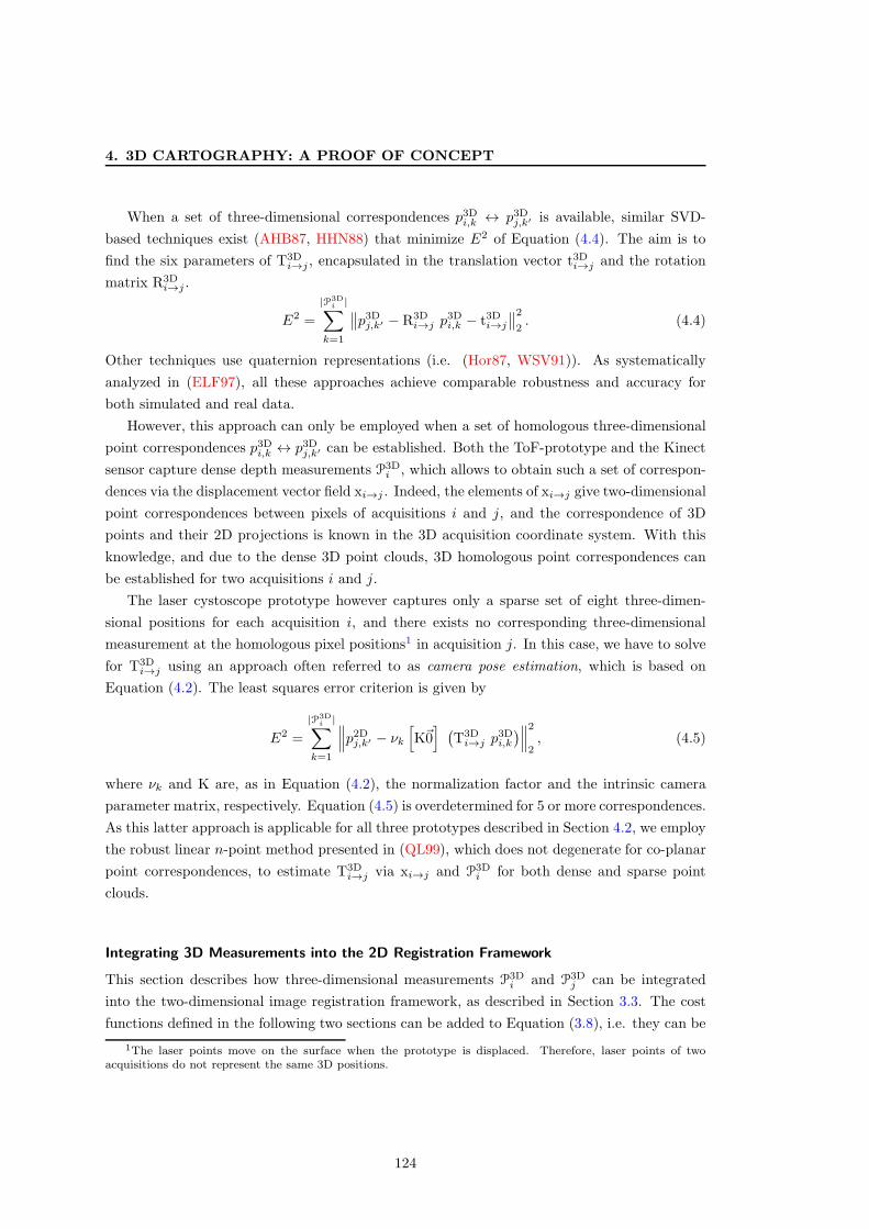
4. 3D CARTOGRAPHY: A PROOF OF CONCEPT
When a set of three-dimensional correspondences p3Di,k ↔ p3Dj,k′ is available, similar SVD-
based techniques exist (AHB87, HHN88) that minimize E2 of Equation (4.4). The aim is to
find the six parameters of T3Di→j , encapsulated in the translation vector t3Di→j and the rotation
matrix R3Di→j .
E2 =
|P3Di |∑
k=1
∥∥p3Dj,k′ − R3D
i→j p3Di,k − t3Di→j
∥∥2
2. (4.4)
Other techniques use quaternion representations (i.e. (Hor87, WSV91)). As systematically
analyzed in (ELF97), all these approaches achieve comparable robustness and accuracy for
both simulated and real data.
However, this approach can only be employed when a set of homologous three-dimensional
point correspondences p3Di,k ↔ p3Dj,k′ can be established. Both the ToF-prototype and the Kinect
sensor capture dense depth measurements P3Di , which allows to obtain such a set of correspon-
dences via the displacement vector field xi→j . Indeed, the elements of xi→j give two-dimensional
point correspondences between pixels of acquisitions i and j, and the correspondence of 3D
points and their 2D projections is known in the 3D acquisition coordinate system. With this
knowledge, and due to the dense 3D point clouds, 3D homologous point correspondences can
be established for two acquisitions i and j.
The laser cystoscope prototype however captures only a sparse set of eight three-dimen-
sional positions for each acquisition i, and there exists no corresponding three-dimensional
measurement at the homologous pixel positions1 in acquisition j. In this case, we have to solve
for T3Di→j using an approach often referred to as camera pose estimation, which is based on
Equation (4.2). The least squares error criterion is given by
E2 =
|P3Di |∑
k=1
∥∥∥p2Dj,k′ − νk
[
K~0] (
T3Di→j p3Di,k
)∥∥∥
2
2, (4.5)
where νk and K are, as in Equation (4.2), the normalization factor and the intrinsic camera
parameter matrix, respectively. Equation (4.5) is overdetermined for 5 or more correspondences.
As this latter approach is applicable for all three prototypes described in Section 4.2, we employ
the robust linear n-point method presented in (QL99), which does not degenerate for co-planar
point correspondences, to estimate T3Di→j via xi→j and P3D
i for both dense and sparse point
clouds.
Integrating 3D Measurements into the 2D Registration Framework
This section describes how three-dimensional measurements P3Di and P3D
j can be integrated
into the two-dimensional image registration framework, as described in Section 3.3. The cost
functions defined in the following two sections can be added to Equation (3.8), i.e. they can be
1The laser points move on the surface when the prototype is displaced. Therefore, laser points of twoacquisitions do not represent the same 3D positions.
124

4.3 3D Cartography Approach
used in any combination with the cost functions defined in the previous chapter. The particular
cost functions used for the results of this chapter are given in Section 4.4.1. However, the energy
cost function extentions for the xi→j vector field determination is only feasible when dense point
clouds (i.e. homologous three-dimensional measurements) are available. Both ToF-prototype
and the Kinect capture such dense point clouds, while for the laser cystoscope prototype, the
following two extensions are not exploitable.
Enforcing Rigid Transformations
The problem of explicit over-smoothing of pairwise regularization terms was addressed in Sec-
tion 3.3.2. A fourth-order potential function allowed to enforce a perspective transformation
globally on the estimated displacement field xi→j . A similar approach that enforces a rigid 3D
transformation can be implemented when (dense) three-dimensional measurements are avail-
able:E♦3D
(xi→j) =∑
(p,k,l,m,n)∈C♦
E♦3D
pklmn(xp, xk, xl, xm, xn) with
E♦3D
pklmn(xp, xk, xl, xm, xn) =∥∥∥T3D♦
klmn p3Di,p − p3Dj,p+xp
∥∥∥
2
2.
(4.6)
T3D♦
klmn in this case is the rigid transformation that transforms the three-dimensional measure-
ments of acquisition i associated with vertices (k, l,m, n) to the three-dimensional measurements
of acquisition j associated with positions (k′, l′,m′, n′). Again, k, l,m and n are chosen to be the
corner vertices in Vr, and all remaining vertices p form fourth-order cliques (p, k, l,m, n) ∈ C♦,
where C♦ is the same set of cliques used for the perspective-enforcing higher-order term of
Equation (3.7). As for the two-dimensional regularization, this ensures a global interaction be-
tween variables. Equation (4.6) will ensure that the displacement vector field xi→j corresponds
to a rigid transformation T 3Di→j : P
3Di → P3D
j .
Scale-Consistent Regularization
Similar to its two-dimensional counterpart E♦(x), the higher-order terms of Equation (4.6)
lead to several non-submodular pairwise terms after reduction. Using three-dimensional mea-
surements P3Di and P3D
j , it is possible to use pairwise regularization, avoiding the problem of
over-smoothing and non-submodular terms. This will lead to an energy function much easier
to minimize. This scale-consistent regularization term is defined as
Escale(xi→j) =∑
(p,q)∈Nr
Escalepq (xp, xq) with
Escalepq (xp, xq) =
(∥∥p3Di,p − p3Di,q
∥∥2−∥∥∥p3Dj,p+xp
− p3Dj,q+xq
∥∥∥2
)2
.
(4.7)
It ensures that the Euclidean distance between the three-dimensional measurements p3Di,p and
p3Di,q is similar to the corresponding Euclidean distance between p3Dj,x+xpand p3Dj,q+xq
. This ensurse
the preservation of the scale of the observed surface parts when passing from one viewpoint to
another.
125
4. 3D CARTOGRAPHY: A PROOF OF CONCEPT
Interpolating Missing Measurements
Both selected vertices p, as well as corresponding positions p + xp might not have valid 3D
measurements in acquisitions i and j. This is the case for non-overlapping parts (i.e. p+xp lies
outside the valid domain of image Ij), and in general for noisy measurements. Such missing
measurements p3Di,p and p3Dj,p+xpare interpolated by fitting a plane equation to the n nearest
available measurements in P3Di and P3D
j with respect to p and p + xp, respectively. In all
experiments, n = 10 was chosen.
4.3.3 Global Map Correction
As argued in Section 3.2, registration of all possible overlapping image pairs in infeasible for
iconic data superimposition algorithms due to time constraints. For this reason, we employ an
extension of the two-dimensional map correction approach to compensate globally accumulated
errors in three-dimensional maps.
First, assuming all consecutive acquisitions have already been registered, global transfor-
mations T3D0→i are obtained via concatenation of local transformation matrices T3D
i→i+1 (see
Equation (4.3)). Then, a subset of additional, non-consecutive image pairs is selected, which
allow to maximize the “material shortcut” (see also Section 3.2). These pairs are then regis-
tered using the algorithm described in Section 3.3 (and potentially with the extensions described
in Section 4.3.2.2 when dense point measurements are available). The combined set of local
(consecutive and non-consecutive) transformations T3Di→j are then used to equally distribute
accumulated 3D point position errors in the global coordinate system.
The following subsections describe only the changes to the algorithm presented in Sec-
tion 3.2.
Detecting Additional Acquisition Pairs
In Equation (3.2), δ2Di,j depicted the percentage of image area overlap between Ii and Ij in the
global two-dimensional coordinate system. Each image was represented by a polygon (rectangle
image domain transformed by T2Di→0) in the global coordinate system, and δ2Di,j was computed
using the area of polygon overlap. Here, we can compute the overlap δ3Di,j between acquisitions
i and j in three-dimensions by projecting the point cloud P3Di into the coordinate system of
acquisition j via T3Di→j , and vice-versa:
δ3Di,j = min
(
|T3Di→j(Pi)|validj
|Pi|,|T3D
j→i(Pj)|validi
|Pj |
)
. (4.8)
In Equation (4.8), |T3Di→j(Pi)|validj is the number of 3D points of acquisition i, whose projections
are valid (i.e. visible) in the two-dimensional coordinate system of Ij , and T3Di→j = T3D
0→jT3D0→i
−1.
All other steps of the algorithm (see Section 3.2.1) remain identical to its two-dimensional
126

4.3 3D Cartography Approach
counterpart, except that the edge weights and the “material shortcut” are computed with δ3Di,jinstead of δ2Di,j . The result is a set of additional non-consecutive acquisition pairs (i → j 6= i)
that have to be registered. Then, all available T3Di→j can be used to find again the shortest path
transformation T3D0→i for each acquisition in the common coordinate system. The edges of this
second graph are also weighted by the SDD between superimposed images Ii, Ij (via T2Di→j as
in Section 3.2.2).
Bundle Adjustment
After global 3D transformations have been updated, errors due to different shortest paths are
present and must be corrected1. In the two-dimensional case, a set of regularly placed grid
points G was created in the global coordinate system of the map. This led to a sparse set
of non-linear equations that allowed to optimize all T2D0→i while minimizing registration errors
jointly for all (consecutive and non-consecutive) T2Di→j .
In three dimensions, creating an equivalent set of regular surface points is not straightforward
due to the sparsity of the point cloud and a lack of neighborhood connectivity2. However, a set
of points P3Di is already available for each acquisition i. These are transformed into the global
coordinate system via T3Di→0(P
3Di ). A simple modification of Equation (3.3) leads to
E2 =
N−1∑
i=0
|P3Di |∑
k=1
1
|Lk|
∑
(i,j)∈Lk
∥∥p3D0,k′ − T3D
j→0T3Di→jT
3D0→i p
3D0,k′
∥∥2
2
, (4.9)
where, as usual, the notation k ↔ k′ indicates that the points expressed in the local coordinate
systems were transformed to the global coordinate system. Equation (4.9) is sparse (20− 30%
non-zero elements in the Hessian matrix), as each global point p3D0,k′ ∈ T3Di→0(P
3Di ) is projected
to valid image coordinates only in a small subset of acquisition pairs Ii and Ij ((i, j) ∈ Lk). The
cost for each point is normalized by the number of acquisitions |Lk|. Again, the parameters
of all global transformation matrices T3D0→i are optimized to minimize the errors induced by
all available local transformations T3Di→j . Just as Equation (3.3), the equation system based
on Equation (4.9) is minimized using a sparse Levenberg-Marquardt routine (Lou10), and the
Jacobian matrix is computed using automatic differentiation (GJM+99).
4.3.4 Contrast-Enhanced Surface Compositing
In Section 3.4, the final textured map was composed by two successive steps, which were both
formulated as energy minimization problems. The first step was designed to correct small
misalignments between overlapping images (by minimizing texture gradients/discontinuities
1For instance, when two point clouds of consecutive acquisitions i and i + 1 are placed into the globalcoordinate system using two different shortest paths, small alignment errors appear between T3D
i→0(P3Di ) and
T3Di+1→0(P
3Di+i).
2One could fit a surface onto the global point cloud, and extract equidistant points.
127

4. 3D CARTOGRAPHY: A PROOF OF CONCEPT
across seams) and to maximize the contrast (by selecting the best possible image index for each
pixel). In the second step of the algorithm, exposure related gradients were attenuated while
retaining contrast and hue of the original images. The discrete two-dimensional domain of the
map allowed to formulate the corresponding equations directly on a pixel-level using the N4
and N8 complementary neighborhood configurations in Equations (3.10) and (3.14).
The point clouds P3Di obtained with the ToF-prototype and the Kinect sensor are generally
noisy and contain holes (see Figure 4.4c and Figure 4.3c). Consequently, it is not straightfor-
ward to extend the compositing algorithm of Section 3.4 to a voxel-level and three-dimensional
complementary neighborhood systems (e.g. N6 and N26). This is even more of a problem
for the laser cystoscope prototype, as it captures only data for eight three-dimensional point
measurements for each acquisition. This leads to a very sparse global point cloud, and many
areas of the observed scene are not covered.
Therefore, to texture the observed three-dimensional measurements, the global point cloud
must first be transformed to an appropriate surface representation. A polygon mesh (consisting
of vertices, edges and faces) is a common representation of (locally) waterproof surfaces that
can be textured. The following section will show how, for N acquisitions, the noisy global point
cloud
P3D =
N−1∑
i=0
T3Di→0(P
3Di )
can be converted to such a polygon mesh, which is known as surface rendering (HDD+92, OS09).
Converting Point Clouds into Meshes
Polygon meshes have been studied extensively in computer graphics and geometric modelling,
and generally different applications require different representations of these meshes. Techni-
cally, faces of a polygon mesh may be represented by triangles, quadrilaterals, simple convex
polygons, or by more general concave polygons (with holes). In this medical application context,
it is sufficient to convert the global point cloud P3D into a triangular mesh, as this simplifies the
texturing process. Let M3D ={V3D,E3D,F3D
}be the polygon representation of the surface
map to be textured, consisting of a set of vertices V3D, edges E3D, and triangular faces F3D.
Depending on the observed scene, different algorithms have to be used to obtain M3D from
P3D. Smooth surfaces without depth discontinuities (such as the bladder phantoms acquired
with the laser cystoscope prototype) allow to compute the polygon mesh M3D using Poisson
reconstruction (KBH06), which yields a very smooth mesh. The algorithm used is available
through the open source system Meshlab (CNR). Required vertex normals are computed using
plane-fitting on each vertex’s nearest neighbors. For scenes that show depth discontinuities (for
instances as shown in Figure 4.4c), Poisson reconstruction is not adequate as it does not handle
sharp discontinuities or multiple objects. For such P3D, we use the classic Marching-Cube al-
gorithm (LC87). Figure 4.5 shows the estimated surface meshes obtained for both scene types.
128

4.3 3D Cartography Approach
(a) (b) (c)
(d) (e) (f)
Figure 4.5: Surface meshes for different scene types. (a) Sparse point cloud, acquired with thelaser cystoscope prototype for a video-sequence of 45 images of a wave phantom. (b) Dense pointcloud of a carpet with waves (35 images), acquired with the Kinect sensor. (c) Dense point cloudfor a scene with discontinuities (single image), acquired with the Kinect sensor. (d)-(e) For sceneswithout depth discontinuities (i.e. smooth surfaces), Poisson reconstruction (KBH06) is used toextract surface meshes. (f) Scenes with depth discontinuities are meshed using marching cubes(LC87). Multiple acquisitions from different viewpoints are necessary to produce a more accuratemesh with less holes.
Note that for scenes with depth-discontinuities, the mesh of a single image contains many holes
and is in general very noisy. Multiple acquisitions from different viewpoints allow to reduce
noise and fill missing surface parts.
Seam Localization on Triangular Meshes
After converting noisy (and potentially locally misaligned due to bladder movement) global
point clouds P3D to a polygon mesh M3D, it is now possible to compute optimized texture.
Similar to Section 3.4.1, the energy function to be minimized is defined as
Eseam3D
(x) =∑
f∈F3D
Eseam3D
f (xf ) + λseam
∑
(f,w)∈E3D
Eseam3D
fw (xf , xw), (4.10)
129

4. 3D CARTOGRAPHY: A PROOF OF CONCEPT
with the configuration
x : F3D → {0, ..., N − 1}
assigning an image index xf to each face f ∈ F3D. As in the two-dimensional algorithm, this
index indicates that the texture for face f is extracted from image Ixf, chosen from the N
images of the sequence. The vertices of f are projected into the images’ coordinate system
via KT3D0→xf
, leading to a projected triangle f2Dxf
in image Ixf. Similar to Equation (3.12), the
contrast of such a triangle projection can then be computed. Instead of using a fixed shape
neighborhood to compute the contrast for a pixel p in the two-dimensional map, Michelson’s
contrast is now evaluated directly within a discrete approximation of f2Dxf
in image Ixf:
Eseam3D
f (xf )=exp
−
maxp∈f2D
xf
Ixf(p)− min
p∈f2Dxf
Ixf(p)
maxp∈f2D
xf
Ixf(p) + min
p∈f2Dxf
Ixf(p)
, (4.11)
where p ∈ f2Dxf
denotes a discrete sampling within the projected face in image Ixf. Like in two
dimensions, a projection with a large contrast will yield a small energy cost, and vice versa.
Texture misalignments are attenuated by minimizing color gradients along the common
edge of neighboring faces. If two faces f, w ∈ F3D share a common edge efw ∈ E3D, the
amount of texture misalignment can be computed by the sum of squared color differences at
the corresponding projected locations along this edge:
Eseam3D
fw (xf , xw) =∑
p3D0,k∈efw
∥∥∥Ihpxf
(p2Dxf ,k′)− Ihpxw(p2Dxq,k′)
∥∥∥
2
2· T (xf 6= xw). (4.12)
The notation p3D0,k ∈ efw denotes a discrete 3D point sampling along edge efw, and p2Dxf ,k′ cor-
responds to the position of each sample projected into image Ixf. As before, the notation
k and k′ indicate the correspondence of a point in different coordinate systems. When two
faces are assigned the same image indices (xf = xw), the truncation function T (·) is null and
Eseam3D
fw (xf , xw) does not contribute to the regularization costs. The use of high-pass filtered
images Ihp (computed with Equation (3.9)) ensures that only texture misalignments are penal-
ized, while exposure related gradients are treated separately in the next section. It is recalled
that in the high-pass filtered images, the texture remains visible, while exposure gradients are
strongly attenuated (for details see Section 3.4.1). Equation (4.10) is minimized using alpha-
expansion until convergence, usually requiring two full cycles over L = {0, ..., N − 1}.
A similar approach was first published in (LI07). While the authors employ the same
strategy for the regularization term, the data term for each face is based on a different quality
criterion. In (LI07), a projection is assumed to be of good quality (i.e. low Eseam3D
f (xf )) when
the angle between face normal and local (in xf ) camera viewing direction (i.e. Z -axis of the
camera) is small. While this approach can be useful for arbitrary viewpoints, it can be neglected
for bladder cartography, as the camera’s Z -axis is close to perpendicular for most acquisitions.
Furthermore, the data term proposed in Equation (4.11) evaluates the quality of a projection
130
4.3 3D Cartography Approach
directly from the image texture. This allows to discard blurry images, and to maximize the
contrast of the textured surface. Similar to two-dimensional seam localization, the method
of (LI07) neglects the problem of motion blur and de-focus and assumes a sequence of well-
contrasted images with small upto moderate exposure differences. As shown in Chapters 1 and
3, this assumption is not valid in cystoscopy.
Exposure and Vignetting Correction
Similar to the two-dimensional case, exposure related color gradients across neighboring faces
can be corrected using blending/feathering techniques (RCMS99, LHS01, Bau02), seam-leveling
(LI07), or total-variation based super-resolution techniques (GC09). However, these approaches
correct exposure differences at the expense of loss of contrast, or can only be used to correct
small exposure differences. As exposure differences are strong in a cystoscopic video-sequence
(see Section 1.3.4), related color gradients are attenuated by a modified version of the methods
proposed in Section 3.4.2.
The energy function to be minimized is given by Equation (4.13):
Eexp3D
(m) =∑
f∈F3D
Eexp3D
f (mf ) + λexp
∑
(f,w)∈E3D
Eexpfw (mf ,mw), (4.13)
where the configuration m : F3D → L ⊂ R3 assigns each face a multiplicative RGB vector to
correct exposure. This means that the texture for a face f ∈ F3D is obtained by point-wise
multiplication, i.e. the color vector Ixf(p) at each pixel p ∈ f2D
xfis point-wise multiplied by
mf , with xf being the image index assigned to each face f in the previous section. This point-
wise multiplication is expressed with the Hadamard (or Schur) product (Dav62) Ixf(p) ◦mf .
The data term Eexp3D
f is used to adjust the “face brightnesses”, while the regularization term
Eexpfw ensures that the edges of neighbouring faces have no color discontinuities. For clarity, the
regularization term is described prior to the data term.
Visible exposure differences across the common edge of two faces are attenuated using
Eexp3D
fw (mf ,mw) =∑
p3D0,k∈efw
∥∥∥Ixf
(p2Dxf ,k′) ◦mf − Ixw(p2Dxq,k′) ◦mw
∥∥∥
2
2. (4.14)
Equation (4.14) is similar to Equation (4.12), except that the original images instead of high-
pass filtered images are evaluated and the indicator function is omitted. The L2 norm allows
for smooth transitions (i.e. small differences in mf and mw) across faces f and w having been
textured from the same image (i.e. xf = xw), while larger exposure differences across faces
textured from different images (i.e. xf 6= xw) are attenuated. To ensure that m does not change
the hue of the original images noticeably, the following data term is used:
Eexp3D
f (mf ) =
∥∥∥∥∥meanp∈f2D
xf
Ixf(p) ◦mf
|Ixf(p) ◦mf |
−meanp∈f2D
xf
Ixf
|Ixf|
∥∥∥∥∥2
. (4.15)
131

4. 3D CARTOGRAPHY: A PROOF OF CONCEPT
Equation (4.15) ensures that the mean color vector of the original image texture points in the
same direction (in the RGB color cube) than the modified mean color vector. Equation (4.13)
is minimized using fusion-moves, with the same brightness and color variations used in Sec-
tion 3.4.2, and converges when the energy decrease within a fixed interval of fusion-moves
drops below a threshold.
4.4 Results
This section presents results obtained for the three prototypes with the methods proposed in
this chapter. First, in Section 4.4.1, data registration robustness and accuracy (in two and three
dimensions) is assessed. In the remainder of this chapter, the term “registration” corresponds
to the estimation of both T2Di→j and T3D
i→j . Similar, registration accuracy corresponds to devi-
ations of the estimated transformation matrices from the ground truth transformations. The
influence of depth sensor noise (3D point reconstruction errors along the Z -axis of the sensor)
and the number of available reconstructed three-dimensional measurements (per acquisition)
on registration quality are evaluated on simulated phantom data. Global map accuracy is then
assessed in Section 4.4.2 on data sets acquired with the sensors described in Section 4.2, as well
as on non-medical scenes, acquired with the Kinect. Furthermore, the efficiency of the proposed
global map correction algorithm is assessed. In Section 4.4.3, the effectiveness of the proposed
contrast-enhancing surface compositing algorithm is evaluated. This chapter concludes with a
discussion of the contributions made in Section 4.5.
Bladder Phantoms
For the medical prototypes (ToF-prototype and laser cystoscope prototype), two phantoms
with different geometry are used to evaluate the proposed registration and map correction
algorithms. The first phantom (shown in Figure 4.6b) has a cylindrical shape (radius of 3.5
cm), and allows to simulate the bladder’s curvature in a realistic fashion orthogonal to the
cylinder’s main axis (the ideal bladder is ovoidal with a radius of 4-5cm). The second phantom,
consisting of several waves (see Figure 4.6c), simulates extreme cases of local deformation due
of other organs warping the bladder. Indeed, without other organs pushing on the bladder, its
shape is ideally convex (when it is filled with isotonic saline solution). When another organ
pushes against the bladder, its shape becomes concave. The wave simulates an extreme surface
warping with several convex deficit parts. The texture for both medical phantoms consists of a
standard paper printout of a pig bladder photograph (as discussed in Chapter 3, pig and human
bladder tissue is visually very similar).
132

4.4 Results
Figure 4.6: Medical phantoms for the assessment of three-dimensional cystoscopic cartography.(a) Pig bladder photograph used to texture the phantoms. The bladder photography correspondsto the upper left quarter of the image. The whole textured image was obtained by using thesymmetries of the photography. (b) Cylindrical phantom with radius of 3.5cm, simulating thecurvature of the bladder orthogonal to the cylinder’s main axis. (c) Wave-shaped phantom and thelaser cystoscope prototype, simulating extreme situations of local deformations. The wavelengthcorresponds to 8 cm, and the amplitude measures 1 cm.
4.4.1 2D and 3D Registration Robustness and Accuracy on a SimulatedPhantom
As discussed in detail in Section 3.5, the proposed higher-order data and regularization terms
allowed for robust and accurate estimation of the two-dimensional displacement vector field
xi→j . The fitted perspective transformations T2Di→j led to very small image registration errors
ǫ2Di→j of about 0.25 pixels (defined in Equation (3.15)) for both consecutive (j = i + 1) and
non-consecutive (j > i) image pairs. Three-dimensional registration accuracy of the estimated
transformations T3Di→j can be similarly quantified by the mean three-dimensional registration er-
ror ǫ3Di→j , which measures the accuracy of placing 3D points from viewpoint i into the coordinate
system of viewpoint j:
ǫ3Di→j =1
|P3Di |
∑
p3Di,k
∈P3D⋆
i
∥∥∥T3D⋆
i→jp3Di,k − T3D
i→jp3Di,k
∥∥∥2. (4.16)
In Equation (4.16), ǫ3Di→j is a straightforward extension of the two-dimensional registration error
ǫ2Di→j , where T3D⋆
i→j is the ground truth transformation matrix, and P3D⋆
i is a set of known and
133
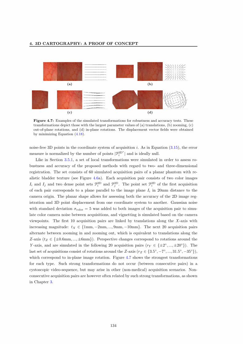
4. 3D CARTOGRAPHY: A PROOF OF CONCEPT
(a) (b)
(c) (d)
Figure 4.7: Examples of the simulated transformations for robustness and accuracy tests. Thesetransformations depict those with the largest parameter values of (a) translations, (b) zooming, (c)out-of-plane rotations, and (d) in-plane rotations. The displacement vector fields were obtainedby minimizing Equation (4.18).
noise-free 3D points in the coordinate system of acquisition i. As in Equation (3.15), the error
measure is normalized by the number of points |P3D⋆
i | and is ideally null.
Like in Section 3.5.1, a set of local transformations were simulated in order to assess ro-
bustness and accuracy of the proposed methods with regard to two- and three-dimensional
registration. The set consists of 60 simulated acquisition pairs of a planar phantom with re-
alistic bladder texture (see Figure 4.6a). Each acquisition pair consists of two color images
Ii and Ij and two dense point sets P3Di and P3D
j . The point set P3Di of the first acquisition
of each pair corresponds to a plane parallel to the image plane Ii in 20mm distance to the
camera origin. The planar shape allows for assessing both the accuracy of the 2D image reg-
istration and 3D point displacement from one coordinate system to another. Gaussian noise
with standard deviation σcolor = 5 was added to both images of the acquisition pair to simu-
late color camera noise between acquisitions, and vignetting is simulated based on the camera
viewpoints. The first 10 acquisition pairs are linked by translations along the X -axis with
increasing magnitude: tX ∈ {1mm,−2mm, ..., 9mm,−10mm}. The next 20 acquisition pairs
alternate between zooming in and zooming out, which is equivalent to translations along the
Z -axis (tZ ∈ {±0.6mm, ...,±6mm}). Perspective changes correspond to rotations around the
Y -axis, and are simulated in the following 20 acquisition pairs (rY ∈ {±2◦, ...,±20◦}). The
last set of acquisitions consist of rotations around the Z -axis (rZ ∈ {3.5◦,−7◦, ..., 31.5◦,−35◦}),
which correspond to in-plane image rotation. Figure 4.7 shows the strongest transformations
for each type. Such strong transformations do not occur (between consecutive pairs) in a
cystoscopic video-sequence, but may arise in other (non-medical) acquisition scenarios. Non-
consecutive acquisition pairs are however often related by such strong transformations, as shown
in Chapter 3.
134

4.4 Results
0 5 10 15 20 25 30 35 40 45 50 55 600
0.5
1
1.5
2
2.5
3
3.5
4
Acquisition pair #
ǫ2D
i→j
[pix
el]
L2
Scale−consistenttztx
ryrz
Figure 4.8: Accuracy and robustness of different pairwise regularization terms. The horizontallabeled lines depict the acquisition pair indices for which a particular rigid three-dimensionaltransformation type (tZ , tZ , ry or rZ) is applied. For transformations without large displacementdifferences between neighboring vertices, 2D data registration accuracy is comparable. For strongzooming or in-plane rotations however, the pairwise regularization of Equation (3.6) convergesto poor local minima, which leads to high out-of-chart registration errors. The scale-consistentregularization term of Equation (4.7) does not lead to pool local minima, and robustly registerseven strong transformations.
Registration Robustness with and without 3D Measurements
In this test, the robustness of the L2 pairwise regularization term of Equation (3.6), as used
for consecutive images in Chapter 3, is compared with that of the scale-consistent pairwise
regularization, formulated in Equation (4.7). For this comparison, Equation (4.17) corresponds
to the energy computed with the L2 pairwise registration term E↔(xi→j), while Equation (4.18)
represents the energy computed with the scale consistent term Escale(xi→j). For both energies,
the second-order data term E△(xi→j) of Equation (3.4) is used.
Ereg2D(xi→j) = E△(xi→j) + λL2 E↔(xi→j) (4.17)
Ereg3D(xi→j) = E△(xi→j) + λscale Escale(xi→j) (4.18)
The parameter λL2 = 1 is set to the constant value used for all results in Chapter 3, while the
parameter λscale = 5 will be used for the experiments in the remainder of this chapter. For
this test, Gaussian noise (standard deviation σdepth = 1mm) was applied to P3Di to simulate
depth sensor noise. This noise level is representative of the three-dimensional point recon-
struction errors of both the ToF-prototype and the laser cystoscope prototype. Looking at
Figure 4.8, it can be seen that the accuracy of 2D registration is comparable for both regu-
larization terms. A blue curve depicts the registration error ǫ2Di→j when using scale-consistent
regularization (Equation (4.18)), while the red curve corresponds to registration errors using L2
pairwise regularization (Equation (4.17)). It is noticeable that for both curves, the ǫ2D values
are mostly smaller than 1 pixel, which is not visually perceptible between two images. For
135

4. 3D CARTOGRAPHY: A PROOF OF CONCEPT
transformations with small magnitudes, the errors are similar (i.e. ǫ2Di→j < 0.4 pixels) to those
obtained on simulated two-dimensional phantoms (see Section 3.5.1).
However, the transformations tested here also correspond to strong transformations, which
often occur between non-consecutive images (notably for large scale and perspective changes).
For transformations that involve large pairwise L2 regularization costs, such as strong zooming
(acquisitions 24-31) or in-plane rotation (acquisitions 55-60), the registration converges to very
incorrect local minima, indicated by the out-of-chart high values of the red curve. Such trans-
formations are often observed for non-consecutive image pairs, as shown in Chapter 3. This fact
led to the development of perspective-invariant higher-order regularization in Section 3.3.2. In-
stead of higher-order terms, the scale-consistent pairwise regularization term can be used when
dense three-dimensional point measurements are available. This leads to faster computation
and less non-submodular terms. The red curve of Figure 4.8 indicates the best results which
can be obtained when dense point measurements are not available for each acquisition, and
the L2 pairwise regularization term of Equation (3.6) has to be used. This is the case for the
laser cystoscope prototype. These results suggest that the higher-order perspective-invariant
regularization of Equation (3.7) should be employed when it is not possible to register non-
consecutive image pairs using dense three-dimensional point measurements, but can be avoided
when such information is available. In fact, using the three-dimensional rigid-enforcing ver-
sion of Equation (3.7), as defined in Equation (4.6), leads to very similar results than those
obtained with pairwise three-dimensional regularization. Because of this, and the increased
algorithmic complexity and number of non-submodular terms, Equation (4.6) was not used in
the experiments.
Registration Accuracy with Varying Sensor Noise Levels
For the second test, increasing Gaussian noise (σdepth = 1, 2, ..., 5 mm) was applied to P3Di
and P3Dj to simulate (strong) depth sensor inaccuracies. Figure 4.9 shows the effect of this
noise on image registration (ǫ2D) as well as on 3D point alignment (ǫ3D) accuracy between
two viewpoints. For this test, only the result of minimizing the energy of Equation (4.18) is
evaluated, as Equation (4.17) is not based on three-dimensional measurements. Increasing depth
noise σdepth leads to monotonically increasing ǫ3Di→j registration errors, as shown in Figure 4.9a.
Dashed lines depict the median registration error for all acquisition pairs of the sequence.
However, noise with a standard deviation of 2 mm or more (in 20 mm distance to the surface)
is very high. The ToF-prototype has, for instance, an error with standard deviation of 0.5 cm
(along the Z -axis) at a distance of 25 cm to the surface, while for the laser cystoscope prototype,
σdepth = 1 mm at a distance of 35 mm. It is noticeable on Figure 4.9, that the ǫ3Di→j value is small
for σdepth = 1mm (median ǫ3D = 0.25 mm) and remains sub-millimetric for σdepth = 2mm (at a
distance of about 20mm). Moreover, depth sensor noise does not have a strong influence on 2D
data registration. As can be seen in Figure 4.9b, the 2D registration error ǫ2Di→j does not increase
136

4.4 Results
0 10 20 30 40 50 600
1
2
3
4
5
Aquisition pair #
ǫ3D
i→j
[mm
]
sigma = 1
sigma = 2
sigma = 3
sigma = 4
sigma = 5
(a)
0 10 20 30 40 50 600
0.5
1
1.5
2
2.5
3
Acquisition pair #
ǫ2D
i→j
[pix
el]
(b)
0 10 20 30 40 50 600
0.5
1
1.5
2
2.5
3
Acquisition pair #
ǫ3D
i→j
[mm
]
(c)
Figure 4.9: Influence of depth sensor noise on registration accuracy. (a) Effect of increasingGaussian noise applied to the (dense) depth measurements on three-dimensional point alignmentaccuracy. Dashed lines indicate the median ǫ3D of all acquisition pairs of the sequence. (b)Two-dimensional registration error does not increase linearly with σdepth. (c) Registration ac-curacy ǫ3Di→j comparison of dense (solid lines) and sparse (dashed lines) depth measurements forσdepth ∈ {1(blue), 3(red)}. While two-dimensional registration accuracy (i.e. the displacementvector field xi→j) is comparable (unlike robustness, see Figure 4.8), three-dimensional inaccuracygrows exponentially for sparse measurements relative to depth measurements with increasing noiseσdepth.
137

4. 3D CARTOGRAPHY: A PROOF OF CONCEPT
(a) (b)
Figure 4.10: Registration of non-consecutive acquisition pairs using scale-consistent regulariza-tion. (a) Example of a registered non-consecutive pair, acquired with the Kinect sensor, showinga curved carpet. (b) Example of a registered pair of a wave phantom, acquired with the ToF-prototype. The displacement vector fields xi→j are smooth, and two-dimensional image super-impositions are accurate for both sensor types. The three-dimensional registration error dependsmainly on the quality and quantity of depth measurement.
monotonically, and is mostly influenced by the magnitude of the transformations, as it is the
case for L2 regularization terms. This result indicates that the scale-consistent regularization
is robust against sensor noise with regard to 2D registration accuracy, while being more robust
with regard to registration success compared to L2 regularization (see also Figure 4.8).
Registration Accuracy of Dense and Sparse Depth Measurements
The final test evaluates the influence of the number of depth measurements (per acquisition) on
three-dimensional registration accuracy for varying depth sensor noise. As can be seen in Fig-
ure 4.9c, the three-dimensional registration error increases exponentially with the noise level
when using sparse measurements (dashed lines), while for dense point measurements (solid
lines), this increase is less severe. For this test, the displacement vector field obtained from
minimizing Equation (4.18) was used to obtain T3Di→j for dense measurements, while the dis-
placement vector field of minimizing Equation (4.17) has to be used for sparse measurements.
The sparse set of measurements corresponds to a spatially well distributed subset of the dense
simulated measurements (see Figure 4.2b).
Conclusions
These results allow to reason that the scale-consistent regularization term is well suited for the
registration of RGB-Depth images (acquired with dense depth measuring prototypes, such as
the Kinect or the ToF-prototype). Even strong transformations (such as zooming, or in-plane
rotations) can be robustly registered (as opposed to image registration with L2 regularization),
which makes this term especially suitable for the registration of non-consecutive image pairs.
At the same time, for moderate transformations, the 2D registration accuracy with the scale-
invariant regularization term is comparable with that of L2 regularization, and the registration
is not particularly sensitive to depth measurement noise. In other words, depth noise does not
have a significant effect on the estimated displacement vector field xi→j obtained by minimizing
138

4.4 Results
Equation (4.18), as shown in in Figures 4.7 and 4.10. The displacement vector fields are smooth,
and correctly superimpose the image pairs in two dimensions. Despite all these advantages, the
three-dimensional registration accuracy strongly depends on the quality of the reconstructed
depth measurements, as these are used to fit T3Di→j . This is especially critical for the laser
cystoscope prototype, as the small number of reconstructed point leads to exponentially larger
inaccuracies, especially when local scene geometry is poor, as will be shown in the next section.
4.4.2 Global Map Reconstruction Accuracy
As in the two-dimensional cartography process, global transformations T3D0→i are obtained by
concatenation of local consecutive transformations T3Di→i+1. These global transformations allow
to place each local point cloud P3Di into the global coordinate system via T3D
i→0(P3Di ). The
accuracy of a two-dimensional global panoramic image is directly related to the accuracy of
the displacement vector field xi→j . As shown in the previous section, the (local and global)
accuracy of three-dimensional point alignment mainly depends on sensor noise, as well as the
number of depth measurements per acquisition. Increasing noise levels lead to monotonically
increasing ǫ3Di→j , and a sparse set of measurements infers exponentially larger errors than dense
measurements. In this section, the effects of accumulated errors on map reconstruction accuracy
and the efficiency of the global map correction technique are evaluated.
Wave Phantom and ToF-Prototype
The first example corresponds to a scan of the wave-shape phantom, recorded with the ToF-
prototype. Figure 4.11a shows the phantom and the acquisition geometry for this setup. The
sequence corresponds to a loop scenario, and consists of 70 manually displaced acquisitions, with
varying translations along X - and Z -axis, as well as rotations around the Y -axis. Acquisition
beginning (image I0), trajectory and ending (image IN−1) are annotated in Figure 4.11a. The
initial point cloud without global correction (only T3Di→i+1 were used) in Figure 4.11c shows
clearly the globally accumulated error when the prototype returns close to the initial position.
Between the three-dimensional points of the first and the last acquisition of the sequence,
this accumulated error corresponds roughly to 1.5 cm, at a distance of 22 cm between optical
center and surface. An area of 20× 13 cm2 is observed during the sequence. After a subset of
additional acquisition pairs has been detected and global map correction has been performed,
the corrected global point cloud, as shown in Figure 4.11d, is free of misalignments. The final
textured surface is shown in Figure 4.11b, which corresponds to the observed surface part of the
phantom, as indicated by the black rectangle in Figure 4.11a. The used ToF-prototype exhibits
a depth measurement error with standard deviation of roughly ±0.5cm at 25 cm distance to
139
4. 3D CARTOGRAPHY: A PROOF OF CONCEPT
the surface. However, due to dense (pixel-wise) measurements and strong depth variations1
seen in each FOV, local errors are relatively small and do not lead to strong inaccuracies when
fitting T3Di→j . In particular, the reconstructed wave is not “bent”, and the measured wavelength
of Figure 4.11b corresponds to 78.6 mm (average taken from several manual measurements),
whereas the true wavelength is known to be 80 mm. The measured amplitude corresponds to
about 9.2 mm, compared to the true amplitude of 1cm. Such errors are insignificant, as the
deformations of the bladder between (and locally during) examinations are larger and therefore
impede very exact measurements.
1The term ”strong depth variations” means here that for each viewpoint, the sensor acquires “rich” geomet-rical information, as the amplitude of the wave phantom is 1cm and at least one wave period is visible in eachFOV. As shown later, local alignment errors are larger for shapes with less depth variations visible in the FOV.
140
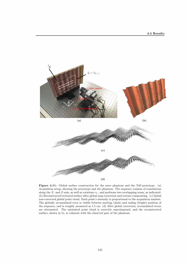
4.4 Results
I0 ∼ IN−1
IN2
tXtZ
rY
Color camera
ToF camera
ToF-IR Wave Projector
(a) (b)
(c)
(d)
Figure 4.11: Global surface construction for the wave phantom and the ToF-prototype. (a)Acquisition setup, showing the prototype and the phantom. The sequence consists of translationsalong the X - and Z -axis, as well as rotations rY , and performs two overlapping scans, as indicated.(b) Reconstructed textured surface after global map correction and texture compositing. (c) Initialnon-corrected global point cloud. Each point’s intensity is proportional to the acquisition number.The globally accumulated error is visible between starting (dark) and ending (bright) position ofthe sequence, and is roughly measured as 1.5 cm. (d) After global correction, accumulated errorsare attenuated. The optimized point cloud is correctly superimposed, and the reconstructedsurface, shown in b), is coherent with the observed part of the phantom.
141
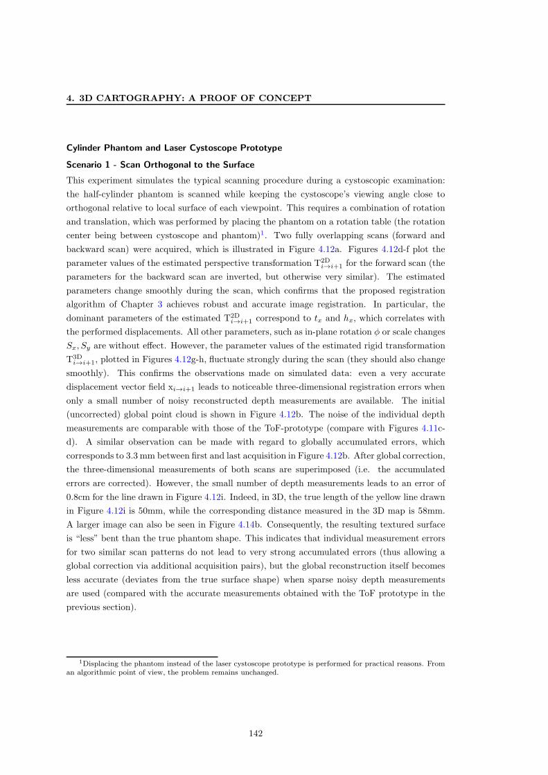
4. 3D CARTOGRAPHY: A PROOF OF CONCEPT
Cylinder Phantom and Laser Cystoscope Prototype
Scenario 1 - Scan Orthogonal to the Surface
This experiment simulates the typical scanning procedure during a cystoscopic examination:
the half-cylinder phantom is scanned while keeping the cystoscope’s viewing angle close to
orthogonal relative to local surface of each viewpoint. This requires a combination of rotation
and translation, which was performed by placing the phantom on a rotation table (the rotation
center being between cystoscope and phantom)1. Two fully overlapping scans (forward and
backward scan) were acquired, which is illustrated in Figure 4.12a. Figures 4.12d-f plot the
parameter values of the estimated perspective transformation T2Di→i+1 for the forward scan (the
parameters for the backward scan are inverted, but otherwise very similar). The estimated
parameters change smoothly during the scan, which confirms that the proposed registration
algorithm of Chapter 3 achieves robust and accurate image registration. In particular, the
dominant parameters of the estimated T2Di→i+1 correspond to tx and hx, which correlates with
the performed displacements. All other parameters, such as in-plane rotation φ or scale changes
Sx, Sy are without effect. However, the parameter values of the estimated rigid transformation
T3Di→i+1, plotted in Figures 4.12g-h, fluctuate strongly during the scan (they should also change
smoothly). This confirms the observations made on simulated data: even a very accurate
displacement vector field xi→i+1 leads to noticeable three-dimensional registration errors when
only a small number of noisy reconstructed depth measurements are available. The initial
(uncorrected) global point cloud is shown in Figure 4.12b. The noise of the individual depth
measurements are comparable with those of the ToF-prototype (compare with Figures 4.11c-
d). A similar observation can be made with regard to globally accumulated errors, which
corresponds to 3.3 mm between first and last acquisition in Figure 4.12b. After global correction,
the three-dimensional measurements of both scans are superimposed (i.e. the accumulated
errors are corrected). However, the small number of depth measurements leads to an error of
0.8cm for the line drawn in Figure 4.12i. Indeed, in 3D, the true length of the yellow line drawn
in Figure 4.12i is 50mm, while the corresponding distance measured in the 3D map is 58mm.
A larger image can also be seen in Figure 4.14b. Consequently, the resulting textured surface
is “less” bent than the true phantom shape. This indicates that individual measurement errors
for two similar scan patterns do not lead to very strong accumulated errors (thus allowing a
global correction via additional acquisition pairs), but the global reconstruction itself becomes
less accurate (deviates from the true surface shape) when sparse noisy depth measurements
are used (compared with the accurate measurements obtained with the ToF prototype in the
previous section).
1Displacing the phantom instead of the laser cystoscope prototype is performed for practical reasons. Froman algorithmic point of view, the problem remains unchanged.
142

4.4 Results
I42
I21
I0
(a)
(b)
(c)
0 20 40−20
−15
−10
−5
0
5
Acquisition #
t x t y [pix
el]
txty
(d)
0 10 20 30 40
0
1
2
3
4
x 10−5
Acquisition #
h x, hy
hx
hy
(e)
0 10 20 30 40
0
0.5
1
Acquisition #S
, phi
[deg
ree]
phiscale
(f)
0 20 40−0.5
0
0.5
1
Acquisition #
t X, t
Y, t
Z [m
m]
tX
tY
tZ
(g)
0 20 40
−2
−1
0
1
Acquisition #
r X, r
Y, r
Z [d
egre
e]
rx
ry
rz
(h) (i)
Figure 4.12: Global surface construction for the half cylinder phantom and the laser cystoscopeprototype. (a) Acquisition setup. The prototype displacements correspond to a combination ofrotation around the Y -axis and translation along the X -axis. The viewpoint is close to perpendic-ular during the sequence, which simulates the scanning procedure of clinicians. (b) Uncorrectedglobal point cloud. The visible gap between first and last acquisition has an error of 3.3 mm. (c)Corrected point cloud. (d) Estimated two-dimensional translation parameters tx and ty (for thefirst scan upto acquisition i = 42). (e) Estimated two-dimensional perspective parameters hx andhy , and (f) in-plane rotation φ and scale change S = Sx + Sy . The plots of d)-f) illustrate thattwo-dimensional image registration is performed robustly and accurately throughout the sequence.(g) Estimated three-dimensional displacements tX , tY and tZ and (h) rotation parameters rX , rYand rZ . Due to point reconstruction inaccuracies and the low number of reconstructed points peracquisition, the estimation of the three-dimensional transformation parameters is less accurateand varies strongly during the sequence. (i) Reconstructed surface from c) (see also Figure 4.14b).While locally accumulated errors are comparable with the ToF-prototype, the overall reconstruc-tion accuracy is worse. The error along the line drawn in i) is 8 mm (58mm measured, true distance50mm), resulting in a cylinder that is slightly less bent than that of the original phantom.
143

4. 3D CARTOGRAPHY: A PROOF OF CONCEPT
Scenario 2 - Scan Parallel to the Cylinder’s Main Axis
The second experiment illustrates these inaccuracies. Instead of performing two almost identi-
cal forward and backward scans, the phantom is now scanned by two zig-zag patterns parallel
to the cylinder’s main axis, as shown in Figure 4.13a. The prototype displacements correspond
to four partly overlapping linear trajectory scans, with a total of 288 acquisitions. Each of
the four trajectory parts consists of 69 translations of tX = 1mm along the X -axis, which are
performed with a micrometer translation table. Translations tY along the Y -axis (which link
overlapping linear trajectory scans) have been performed manually, because only one transla-
tion table was available. Within each individual trajectory line, the observed three-dimensional
geometry is identical (i.e. noise-free depth measurements would be reconstructed at the same
local coordinates), while it changes between each trajectory. In the first two trajectories (first
zig-zag, acquisition numbers 1 - 150), the observed three-dimensional geometry is relatively
“rich”. As the prototype’s viewing angle is not orthogonal to the surface, visible curvature (as
illustrated by the strong perspective FOVs in Figure 4.13a) leads to depth variations between
the eight reconstructed three-dimensional measurements. These variations impede large inac-
curacies when estimating T3Di→i+1, and the estimated parameters of the rigid transformations
correspond effectively to |tX | =1 mm, as shown in Figures 4.13c-d. The other five parameters
(tY , tZ , rX , rY , rZ , see caption of Figure 4.13) of T3Di→i+1 remain close to 0 (except for tY at the
trajectory turnings).
However, local registration/data alignment errors become stronger when the FOV observes
less three-dimensional structure/depth variations, as is the case for the second zig-zag (acqui-
sition numbers 151-288). These two trajectory scans observe the surface almost orthogonally
to the local viewing direction along the Z -axis, so that the reconstructed depth measurements
do not exhibit strong variations (reconstructed points are situated on a “quasi-planar” local
surface orthogonal to the Z -axis of the camera). Inaccuracies of local depth measurements now
have a stronger influence on the parameters of the estimated T3Di→i+1. As can be seen in Fig-
ures 4.13c-d, the parameter tX is increasingly underestimated in the last two linear trajectory
scans (i.e. |tX | < 1mm). In turn, this is compensated by an overestimation of rY (|rY | > 0◦).
The increasing errors on the estimated rigid transformations T3Di→i+1 correlate with the
initial (uncorrected) global point cloud, as shown in Figure 4.13b. As before, the intensity of
the points are proportional to the acquisition index. Accumulated errors between the trajectory
parts of the first zig-zag scan are relatively low (i.e. comparable with the results obtained with
the ToF-prototype and the orthogonal forward-backward scan), the corresponding parts of
the global point cloud reflect the linear (translation-only) scan paths. However, the points
corresponding to the third and fourth trajectory lines exhibit increasingly stronger deviations
from a linear shape, and accumulated errors become significantly larger (between second and
third trajectory line). Furthermore, the global point cloud is affected by a “bending”-effect due
to the overestimation of rY . As with the forward-backward scan example in the previous section,
accumulated errors between trajectories that observe similar three-dimensional structure (i.e.
144

4.4 Results
I0
IN−1
IN4
I3N4
(a) (b)
0 50 100 150 200 250 300−2
−1
0
1
Acquisition #
t[m
m]
tX
tY
tZ
(c)
0 50 100 150 200 250 300−1
0123
Acquisition #
r[◦
]
rXrZrZ
(d)
−60
−40
−20
001020
−5
0
5
10
15
20
25
30
35
40
y [mm]
x [mm]
z[m
m]
P3D0
P3D287
(e)
−70−60
−50−40
−30−20
−100
010
20
0
10
20
30
x [mm]y [mm]
z[m
m]
P3D0
P3D287
(f)
(g) (h)
Figure 4.13: Global surface construction for a cylindrical bladder phantom and the laser cysto-scope prototype. (a) The sequence simulates two zig-zag paths, as indicated by the green lines.The last two scan-lines exhibit poor local depth information (the reconstructed points lie in a planeorthogonal to the camera’s Z -axis) (b) Initial (non-corrected) global point cloud, exhibiting largeaccumulated errors. (c) Translation parameters of the estimated transformations. (d) Rotationparameters. As can be seen in c) and d), with decreasing depth variation in the FOV, translationsare underestimated, while rotations are overestimated. (e) Additional pairs (thick red lines) usedfor global map correction are nonetheless found. (d) Scene geometry after global correction. (g)Corrected point cloud: accumulated errors are attenuated. (h) Left image: reconstructed texturedsurface viewed roughly from the same viewpoint than a). Right image: half-cylinder part viewedfrom the side. The cylindrical shape is clearly visible, and sufficient for the medical applicationcontext.
145

4. 3D CARTOGRAPHY: A PROOF OF CONCEPT
first and second, respectively third and fourth trajectories) are lower than those between second
and third trajectory scans. This indicates that when using the laser cystoscope in a clinical
situation, relative errors between partly overlapping trajectory scans can be kept (relatively)
low, as long as the cystoscope is displaced at a similar angle towards the observed surface.
While this is usually the case (as clinicians mostly navigate orthogonally to the surface), clinical
examinations are required in order to verify the observations made here.
Despite the relatively strong alignment errors between the different trajectories of this ex-
periment (compared to the previous experiments), correct additional acquisition pairs were
found (see Figure 4.13e). After global correction, the corresponding point cloud is free of local
misalignments, as shown in Figures 4.13f-g. The textured surface is shown in Figure 4.13h,
and corresponds visually to the part of the observed cylinder phantom (see Figure 4.13a),
both in texture and shape. As explained previously, an exact reconstruction of the bladder is
not required in cystoscopy, as the shape of the bladder changes between (and locally during)
examinations. It is only important to preserve the overall shape and texture continuities.
Comparison with (BHDS+10)
Figure 4.14 shows that, for moderate cystoscope displacements and depth variations visible
in the FOV1, the method proposed in (BHDS+10) is unable to accurately estimate the rigid
three-dimensional transformation T3Di→j . The assumptions made in (BHDS+10) about the two-
dimensional perspective relation between overlapping images do not hold in the phantom ac-
quisition scenario, previously assessed and shown in Figure 4.12. The images do show minor
depth variations of the cylinder phantom (see the FOV illustration in Figure 4.12a), so a per-
spective transformation T2Di→j only approximates the actual non-linear transformation between
consecutive image pairs. As the method of (BHDS+10) optimizes the parameters of T3Di→j
by minimizing image dissimilarity between Ij and T2Di→j(Ii), the simplex-driven optimization
estimates mainly translations, unable to recover also the rotation part of the underlying pro-
totype displacements, as can be seen in Figure 4.14a. The displacement vector field xi→j is
estimated independently of any assumptions about 2D image geometry. This allows to esti-
mate both rotation and translation of the prototype displacements. It should be noted that the
method proposed in (BHDS+10) registers every image pair of the 24fps video-sequence, whereas
the methods proposed in this thesis use only every tenth image. Consequently, the method of
(BHDS+10) will work more accurately for very low displacements (large image overlap), and/or
when the cystoscope is closer to the epithelium. However, this cannot be always guaranteed,
and non-consecutive acquisition pairs cannot be robustly and accurately registered with this
method.
1During a cystoscopic examination, the endoscope is often, but not systematically, displaced slightly closer tothe epithelium. Only for short distances between cystoscope and epithelium, the FOV is small and correspondsto weak depth variations.
146

4.4 Results
(a) (b)
Figure 4.14: Comparison with the method proposed in (BHDS+10). (a) Point cloud alignedwith the proposed method (increasing grey values) and with the method of (BHDS+10) in blackfor the forward scan of Figure 4.12, shown in the same global coordinate system of acquisitioni = 0. The assumptions made in (BHDS+10) concerning the two-dimensional geometry betweenoverlapping acquisitions does not hold (i.e. the FOV corresponds to non-planar surface parts).The simplex-driven optimization method of (BHDS+10) is unable to estimate the rotation partof the prototype displacements and estimates only translations. The point cloud consequently isnot bent. Our method makes no assumptions about 2D geometry, and the non-linear deformationfield xi→j allows for estimating both translations and rotations (see Figure 4.12 and text forthe performed prototype displacements). (b) Larger view of the final textured surface shown inFigure 4.12i.
Non-Medical Scene Reconstruction with the Kinect Sensor
A flat textured carpet is captured with the Kinect sensor as the first example, being of similar
locally smooth appearance than the bladder phantoms. The initial (non-corrected) point cloud,
shown in Figure 4.15a, is less noisy than those obtained with the ToF prototype (see Figure 4.11)
or the laser cystoscope prototype (Figure 4.13). Even without global map correction, the
points of different acquisitions are already well aligned and of planar appearance (i.e. without
visible misalignments). In fact, the globally corrected point cloud and the non-corrected one
are visually almost indistinguishable, so we choose to show only the latter here. Figure 4.15b
shows the same cloud, viewed from the top. The density of the cloud indicates which areas were
captured from several trajectory parts (viewpoints). For instance, the top-left part is visited
several times, while the central part is visited by two trajectories (central trajectory, plus the top
and bottom parts, respectively). The complete acquisition path is shown in Figure 4.15c. Found
additional pairs are again indicated by thick red lines (refer to Figure 4.13 for explanations).
Finally, a full 360◦ scan of the author’s living room was acquired with the Kinect sensor.
To do so, the Kinect was rotated manually in the center of the room. Figure 4.16 shows a few
viewpoints of the reconstructed, globally corrected point cloud.
147
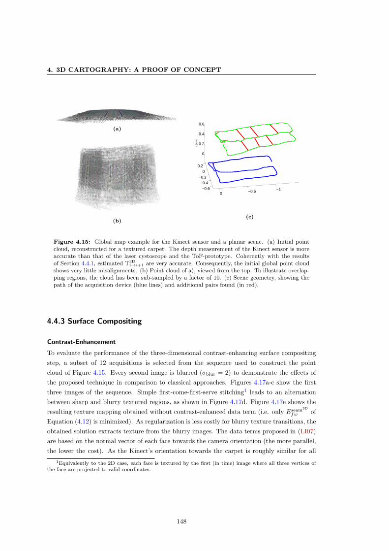
4. 3D CARTOGRAPHY: A PROOF OF CONCEPT
(a)
(b)
−0.6−0.4
−0.20
0.2
−1−0.50
0
0.2
0.4
0.6
z[m
m]
(c)
Figure 4.15: Global map example for the Kinect sensor and a planar scene. (a) Initial pointcloud, reconstructed for a textured carpet. The depth measurement of the Kinect sensor is moreaccurate than that of the laser cystoscope and the ToF-prototype. Coherently with the resultsof Section 4.4.1, estimated T3D
i→i+1 are very accurate. Consequently, the initial global point cloudshows very little misalignments. (b) Point cloud of a), viewed from the top. To illustrate overlap-ping regions, the cloud has been sub-sampled by a factor of 10. (c) Scene geometry, showing thepath of the acquisition device (blue lines) and additional pairs found (in red).
4.4.3 Surface Compositing
Contrast-Enhancement
To evaluate the performance of the three-dimensional contrast-enhancing surface compositing
step, a subset of 12 acquisitions is selected from the sequence used to construct the point
cloud of Figure 4.15. Every second image is blurred (σblur = 2) to demonstrate the effects of
the proposed technique in comparison to classical approaches. Figures 4.17a-c show the first
three images of the sequence. Simple first-come-first-serve stitching1 leads to an alternation
between sharp and blurry textured regions, as shown in Figure 4.17d. Figure 4.17e shows the
resulting texture mapping obtained without contrast-enhanced data term (i.e. only Eseam3D
fw of
Equation (4.12) is minimized). As regularization is less costly for blurry texture transitions, the
obtained solution extracts texture from the blurry images. The data terms proposed in (LI07)
are based on the normal vector of each face towards the camera orientation (the more parallel,
the lower the cost). As the Kinect’s orientation towards the carpet is roughly similar for all
1Equivalently to the 2D case, each face is textured by the first (in time) image where all three vertices ofthe face are projected to valid coordinates.
148

4.4 Results
(a) (b)
(c)
Figure 4.16: Full 360 degree scan of a living room with a hand-held Kinect. (a) Globallycorrected global point cloud viewed from the top. The points are globally well aligned (i.e. theroom is rectangular, and all walls are connected). (b) Same cloud, viewed from the position of thetelevision. (c) Viewed from the right door seen in b).
12 acquisitions, the method of (LI07) can be assumed to produce a comparable, blurry texture
mapping. After minimizing both regularization and contrast-enhanced data terms proposed in
this chapter, the texture is taken from the sharp images of the sequence, while at the same time
being visually coherent, as can be seen in Figures 4.17f-g.
Comparison with the Kinect-Fusion Algorithm
The proposed surface texturing approach is also suitable for more general 3D scenes. We
demonstrate this on a scan of a desktop, reconstructed with the Kinect-Fusion algorithm
(NDI+11, IKH+11). The implementation of this algorithm was taken from the open source
Point Cloud Library (PCL) (RC11). In essence, the Kinect-Fusion algorithm performs real-
time registration of each current P3Di into a fixed-size 3D volume via ICP running on the GPU.
The volume itself is represented as a truncated signed distance function (CL96) and kept in
GPU memory throughout the acquisition. Each registered point cloud is used to iteratively
update the volume. The main limitation of this real-time implementation is the relatively low
149

4. 3D CARTOGRAPHY: A PROOF OF CONCEPT
(a) (b) (c)
(d) (e)
(f) (g)
Figure 4.17: Contrast enhancement for textured surfaces. (a)-(c) Three of 12 input images ofthe carpet sequence used to construct the map of Figure 4.15. Every second image is stronglyblurred to demonstrate the effects of the proposed method. (d) Initial surface texture (first come,first serve). Note how blurry and contrasted images are interlaced. (e) Surface texture determinedwithout contrast-enhancing data term. Color gradients are less strong in blurry images. (f)Surface textured using contrast-enhancing data term. Most of the texture is obtained from thesharp images of the sequence. (g) Exposure correction of f).
spatial resolution of the volume, which is limited by the memory of the graphics card. In our
experiments, the largest resolution that could be used1 was a 256× 256× 256 voxel volume.
Figures 4.18a-c show three of 36 images of the RGB-Depth sequence used. During the
acquisition stage, the Kinect was moved around the desktop, leading to a great variability in
viewpoints. The PCL implementation offers to triangulate a surface mesh on the reconstructed
point cloud. This reconstructed mesh, the images and the camera viewpoints (i.e. T3D0→i) are
1Using an NVIDIA Quadro 600 graphics card with 1GB RAM.
150
4.4 Results
used as the input for the proposed contrast-enhancing surface compositing algorithm, which is
compared qualitatively with both the PCL texturing implementation and a first-come-first-serve
approach. Figure 4.18d shows the texture of the PCL implementation, which chooses the texture
for each face from the first image Ii that projects this face to valid image coordinates. This allows
to push occluded faces to the next acquisition i+1, eventually allowing to label faces that cannot
be projected to valid coordinates in any image as being occluded. As can be seen in Figure 4.18d,
this approach does not necessarily lead to neighboring faces being textured by consecutive
acquisitions. For instance, the checkerboard pattern, the monitors, and most prominently
the keyboard, show visible misalignments due to incorrect estimation of T3D0→i by the Kinect-
Fusion algorithm. Alternatively, the mesh can be iteratively over-textured by the image of the
next consecutive acquisition (first-come-first-serve). This approach is shown in Figure 4.18e.
As local registration errors between consecutive acquisitions are smaller compared to global
transformation inaccuracies, texture misalignments are noticeably reduced. Nonetheless, seam
locations are arbitrary (with respect to scene geometry and texture) and pass through objects
(e.g. the monitors), and still exhibit smaller misalignments. The proposed contrast-enhancing
seam detection algorithm chooses seams in mostly homogeneous areas, as shown in Figure 4.18f.
The monitors and the checkerboard are now textured by single images, leading to overall visually
more coherent texture transitions.
151

4. 3D CARTOGRAPHY: A PROOF OF CONCEPT
(a) (b) (c)
(d) (e)
(f) (g)
Figure 4.18: Contrast-enhancing surface compositing example on a scene constructed with theKinect-Fusion algorithm (NDI+11, IKH+11). (a)-(c) Three of 36 images of the sequence showinga desktop, illustrating the strongly varying viewpoints. (d) Textured scene output of the PCLimplementation (RC11). Note that this texture generation is part of PCL, not the Kinect-Fusionpublication. Each face is textured by the first acquisition that correctly projects this textureinto its image plane. This leads to many misaligned neighboring faces (e.g. the checkerboardpattern, the monitors and the keyboard). Occlusions checks are also performed, leading to holesnoticeable on the desktop. (e) Textured using first-come-first-serve strategy. As registration errorsare small(er) between consecutive images, visible misalignments are reduced (see checkerboard),but still present (monitor edges, screen content). (f) Texture after seam localization. Textures arenow correctly aligned (except for the mouse cable), seams pass homogeneous areas where possible.(g) Exposure correction.
152

4.5 Conclusions and Perspectives
4.5 Conclusions and Perspectives
The methods developed in this chapter correspond to modifications of the two-dimensional
cartography process, as proposed in Chapter 3. As argued in Sections 1.4 and 4.1.2, without
additional sensor information, estimating the rigid instrument displacement is not possible
due to the small FOV and the poor local geometry (depth variation) of cystoscopic video-
sequences. The methods therefore assume that modified instruments (which were introduced in
Section 4.2) allow to capture local three-dimensional information in addition to the color images.
As these prototypes are not yet available in clinical examinations, the results of this chapter
are limited to a proof of concept. Nonetheless, the results obtained for quite realistic (with
regard to shape and texture) phantom data show the potential of the proposed methods. As in
Section 3.5, constant parameters were used for all experiments, demonstrating the robustness
of the proposed algorithms. Additionally, the methods can also be applied to more general
acquisition scenarios, which was demonstrated for a set of scenes acquired with the Kinect
sensor.
In the following sections, we present the main scientific contributions made in this chapter,
and discuss their limitations and potential future work.
4.5.1 Main Scientific Contributions
Robust Data Registration
In Chapter 3, the perspective transformation T2Di→j that links two images of a cystoscopic video-
sequence was computed by solving an over-determined linear system. The rigid transformation
T3Di→j , required for three-dimensional cartography, is similarly estimated. In other words, both
equation systems are based on the two-dimensional displacement vector field xi→j , which gives a
set of correspondences between two acquisitions. Consequently, the data registration algorithm
used to estimate T3Di→j inherits the robustness of its two-dimensional version, described in Sec-
tion 3.3. Robustness and accuracy of the method of (BHDS+10) depend on an initial estimate
of T3Di→j and can therefore only handle consecutive acquisition pairs with small displacements.
The proposed method allows to register both consecutive and non-consecutive acquisition pairs
(needed for global map correction) pairs robustly. In addition, compared to (BHDS+10), the
proposed method does not assume that the acquisition pairs are related by a perspective two-
dimensional transformation T2Di→j . In turn, more general surface geometry can be registered,
such as non-planar scenes (strong local bladder deformations, non-medical scenes).
Compared to classical approaches, the proposed method is able to register acquisition pairs
that exhibit both poor local depth variations and poor texture quality. Poor depth variations
impede the use of classic 3D-3D point registration techniques, such as ICP based algorithms,
while poor texture quality prevents a robust use of feature-based 2D registration algorithms
153

4. 3D CARTOGRAPHY: A PROOF OF CONCEPT
combined with depth sensor measurements. This situation (poor geometry and texture) is often
observed in cystoscopic video-sequences, and the experimental results indicate that a combi-
nation of the registration algorithm proposed in Chapter 3 and modified cystoscopes allow to
robustly estimate viewpoint changes of the cystoscope during the examination. Furthermore,
it was shown that the depth measurements can be integrated in form of pairwise regulariza-
tion into the energy minimization framework of Section 3.3. Unlike classic pairwise L1 or L2
regularization, the integration of dense depth measurements allow to register acquisition pairs
related by arbitrary viewpoint changes without implicit oversmoothing. Therefore, it is not
necessary to use either 2D or 3D higher-order regularization when registering non-consecutive
acquisition pairs.
Global Map Correction
In order to correct globally accumulated cartography errors, the automatic detection of trajec-
tory crossings (zig-zag paths, loops, see Section 3.2) was modified to work on data acquired with
the prototypes used in this chapter. The modified algorithm allows for detecting a meaningful
subset of additional, non-consecutive acquisition pairs. The amount of acquisition overlap is
computed using multiple view geometry formulations. After these additional acquisition pairs
are registered using the method discussed previously, global transformation parameters are
optimized jointly while minimizing local registration errors.
Contrast-Enhanced Surface Compositing
The pixel-based contrast-enhanced map stitching technique, as proposed in Chapter 3, was
extended to a mesh-based surface compositing method. As in the two-dimensional case, blurring
induced by blending techniques, is avoided. At the same time, the quality of the textured surface
is greatly enhanced. This is achieved by preferring contrasted regions in the original images
over blurry ones. The resulting three-dimensional maps are visually coherent and do not exhibit
texture or exposure discontinuities. The two-step compositing approach allows to first maximize
the contrast of the global surface, and attenuate exposure related gradients in a second step.
Compared to state-of-the-art techniques, this allows to reconstruct high contrasted meshes of
the epithelium in the presence of motion blur, and is able to attenuate even very strong exposure
differences.
4.5.2 Limits and Perspectives
As it is the case for the two-dimensional cartography algorithm, the proposed three-dimensional
cartography process requires accumulated errors to be low enough in order to detect additional,
non-consecutive overlapping acquisition pairs. As long as this (moderate) constraint is met,
large FOV textured surfaces can be constructed automatically. When accumulated errors are
too large, a solution is to allow the clinicians to manually select additional overlapping acqui-
sition pairs that cannot be detected automatically from the uncorrected initial map. Such a
154

4.5 Conclusions and Perspectives
(a) (b)
Figure 4.19: Manual loop correction. (a) In extreme situations, overlapping parts cannot bedetected, such as in this full 360 degree scan, performed with the ToF prototype inside a fullcylinder phantom. (b) After manual selection of loop beginning and loop ending, the cylinder canbe reconstructed in a coherent fashion with regards to texture and shape. Note that the visiblevertical texture discontinuities correspond to different sheets of paper with bladder texture.
situation is shown in Figure 4.19. The ToF prototype was manually displaced in a combination
of rotations and translations inside a full cylinder phantom. As can be seen in Figure 4.19a,
the accumulated errors after a full 360 degree scan are too strong. Consequently, loop be-
ginning and loop ending do not overlap at all, and the section of overlap cannot be detected
automatically. After manually choosing the first and the last acquisition as an additional over-
lapping acquisition pair, the full cylinder can be reconstructed in a visually coherent fashion,
as shown in Figure 4.19b. Even in such an extreme scenario1, the required user input is much
less than needed by the method of (BTGA11), and furthermore does not restrict the clinicians
accustomed fashion of scanning the epithelium.
Concerning computation time improvements, the remarks made in Section 3.6 also apply
here. Depending on the images textures, different algorithms for image registration could be
selected. When sufficient image primitives can be extracted, fast feature based approaches could
be used to decrease the overall computation time, while the method proposed in this chapter
may be used as a fall back solution when faster algorithms fail. Prediction techniques, such as
a Kalman filter, could also help to decrease computation time by limiting the search range or
by supplying an initial estimate, depending on the registration algorithm employed.
1The bladder cannot be scanned in such a way with a rigid cystoscope.
155

4. 3D CARTOGRAPHY: A PROOF OF CONCEPT
156

Conclusion
The main objective of this thesis was to facilitate bladder cancer diagnosis using discrete energy
minimization techniques. The proposed large (two- and three-dimensional) FOV maps of the
epithelial surface of the bladder enable clinicians to see multi-focal bladder lesions in their
entirety and with respect to anatomical landmarks. Furthermore, such maps allow for archiving
the examination in an intuitive, re-usable format. Compared to archiving video-sequences, these
maps greatly reduce redundancy, and enable clinicians to compare lesion evolution side-by-side
when preparing for lesion follow-ups. Several previous contributions focused on the creation of
such large FOV maps from cystoscopic video-sequences, including three previous dissertations
at the CRAN laboratory. In the following, the main contributions and perspective of this thesis
are summarized.
Medical Contributions
From a clinician’s point of view, the methods proposed in this thesis lead to several improve-
ments over previous contributions towards bladder cartography. For the first time, large FOV
maps can be constructed from multiple overlapping cystoscope trajectories. Previous contri-
butions presented only “strip”- or “band”-shaped maps with a large FOV in only one main
direction, which severely limits the applicability in clinical situations. The approach proposed
in this thesis is able to create large FOV maps from multiple scan trajectories, thereby extend-
ing the FOV in two directions. Strip-shaped maps, obtained with state-of-the-art methods,
require similar scan-paths for a direct comparison of larger parts of the epithelium. The maps
constructed with the proposed methods potentially enable to compare larger parts of the epithe-
lium from different examinations, without enforcing clinicians to follow a similar scanning path
in a follow-up examination. Furthermore, we have proposed a map compositing approach that
increases the visual quality of the constructed maps. From the redundant data of the video-
sequence, the map texture is composed by a maximum of information and contrast. Motion
blur and camera de-focus is greatly attenuated, and the constructed maps show finer vascular
structures than those presented by previous contributions.
157

Conclusion
Scientific Contributions
These medical contributions required to solve several algorithmic challenges. The corresponding
scientific contributions are summarized in the following paragraphs.
Automatic Global Map Correction. Previous contributions constructed large FOV maps
by concatenating successive images of the video-sequence into the coordinate system of a ref-
erence acquisition. However, as the cystoscope returns to previously visited areas, globally
accumulated errors lead to visible texture misalignment. We have proposed a graph-based
approach to detect such trajectory crossings. Furthermore, our method automatically selects
a small subset of all overlapping non-consecutive acquisition pairs. This greatly reduces the
number of acquisition pairs that need to be registered, while ensuring that all parts of the map
can be corrected. A sparse non-linear bundle adjustment approach then simultaneously adjusts
all transformation parameters, leading to a globally aligned set of acquisitions. This approach
was successfully applied in Chapter 3 for two-dimensional cystoscopic cartography. Results on
simulated and clinical datasets showed that the proposed map correction technique works ro-
bustly, even in the case of larger accumulated errors. Furthermore, the approach was designed
to be extendible to three-dimensional cartography. In Chapter 4, we showed that merely one
equation has to be adapted, namely the computation of acquisition overlap percentage.
Invariant Energy Functions for Data Registration. In Chapter 3, we have proposed data
and regularization cost functions which are invariant to the perspective transformation model
that links overlapping images of a cystoscopic video-sequence. These allow, for the first time
in bladder cartography, for robustly and accurately registering non-consecutive image pairs,
related by arbitrary (and often large) viewpoint changes. Such images have to be registered
in order to achieve global map correction, as described in the previous paragraph. It was
shown quantitatively on simulated phantom data that consecutive image registration accuracy
is superior to state-of-the-art registration techniques. The registration of non-consecutive image
pairs is similarly accurate, while previous contributions cannot even robustly register such
image pairs. The proposed method was successfully applied to several clinical data sets, and
constant algorithm parameters demonstrated the registration robustness. In Chapter 4, it was
shown that the proposed registration approach is also suitable to robustly estimate the rigid
cystoscope displacements when additional sensor information is available. Hence, the method
can directly be used for three-dimensional cartography. Additionally, the cost functions can
be extended to include additional three-dimensional sensor measurements, removing the need
for higher-order regularization. This leads to cost functions that are easier to minimize, which
decreases computation time and algorithmic complexity. Furthermore, no assumption on the
two-dimensional relationship between overlapping images is made. Consequently, the proposed
registration technique is able to estimate the rigid transformation between local acquisition
158

Conclusion
systems even for (locally) non-planar scenes. This was demonstrated using the commercially
available Kinect sensor.
Contrast-Enhancing Map Compositing. We have proposed a two-step map compositing
approach in Chapter 3, which enables to compensate three major problems typical of cysto-
scopic video-sequences. First, small texture misalignments due to local and temporal bladder
deformations remain perceptible after global map alignment. These lead to ghosting and blur
when blending techniques are used, and overall suppress fine vascular structures. Second, mo-
tion blur and camera de-focus are often observed in cystoscopic video-sequence. These lead to a
loss of information (additional blur) in the map when blending techniques are used. Third, due
to vignetting and different viewing angles of the cystoscope towards the epithelium, exposure
differences are strong between overlapping images, especially for non-consecutive image pairs.
The proposed cost functions allow for correcting small misalignments and exposure differences,
while simultaneously minimize the loss of information by choosing the most contrasted images
from the redundant video-sequence. Results on clinical datasets show, both quantitatively and
qualitatively, the improvements compared to previous contributions. Furthermore, the cost
functions were adapted to work on triangular meshes in Chapter 4. On both medical phan-
tom data sets, as well as more general scenes acquired with the Kinect, the method is able to
construct seamless and visual coherent textured surfaces with a maximum of contrast.
Perspectives
As pointed out in the previous section, the proposed techniques contribute in several ways
to the state-of-the-art of constructing two- and three-dimensional large FOV maps of the ep-
ithelium. Nevertheless, some problems remain, and the proposed methods open a few new
perspectives. The criterion that was least considered when developing the cartography algo-
rithms was computation time. Instead, the focus was laid on the development of robust and
accurate algorithms, enabling to compute maps of high visual quality. For these reasons, the
proposed methods, especially the registration part, cannot be used in a real-time application.
However, the computation times allow for a second diagnosis or patient interview after the
examination. Nonetheless, it can be desirable to construct large FOV maps in real-time1, un-
der the restriction that map accuracy and quality does not suffer drastically. One possible
solution to decrease computation time is to use fast registration techniques whenever possible,
and use the proposed method only for difficult (e.g. strong motion blur, non-consecutive, etc.)
image pairs. Such an approach to decrease registration time is currently being evaluated at
the CRAN laboratory. Furthermore, in a real-time application, the proposed sequential car-
tography approach is also not directly usable. For instance, global map correction must be
1Processing times of one or two frames per second should suffice, as in all experiments of this thesis, thecystoscope displacement allowed to process only every tenth image from the 24 fps video-sequences with sufficientoverlap between consecutive image pairs.
159

Conclusion
performed during the acquisition and consecutive image registration stage. Trajectory cross-
ings have to be detected and global transformations must be corrected “on the fly”. However,
the proposed method can easily be modified to work in such a way. The frame structure graph
can be incrementally updated, while re-using most of the already computed edge weights and
shortest-paths. Likewise, the proposed map compositing technique can be modified to work on
a frame-by-frame base. By decreasing the map sections to be corrected (i.e. only update the
map texture in a small region around the current image to be placed in the map), it is possible
to update the map in less than a second. Although shortest path search, global map correction,
and map compositing can be modified to be performed “on the fly”, reaching real-time will
remain a challenge. Nevertheless, these algorithm parts could be processed in a separate thread
(and updated less frequently), while registration and simple map updating can be performed
at faster processing speed.
160

References
[ADA+04] A. Agarwala, M. Dontcheva, M. Agrawala, S. Drucker, A. Colburn, B. Curless,
D. Salesin, and M. Cohen. Interactive digital photomontage. In ACM Transac-
tions on Graphics (TOG), volume 23, pages 294–302. ACM, 2004.
[ADG09] C. Albitar, C. Doignon, and P. Graebling. Calibration of vision systems based
on pseudo-random patterns. In Intelligent Robots and Systems, 2009. IROS
2009. IEEE/RSJ International Conference on, pages 321–326. IEEE, 2009.
[AFG08] A. Ali, A. Farag, and G. Gimelfarb. Optimizing binary mrfs with higher order
cliques. Computer Vision–ECCV 2008, pages 98–111, 2008.
[AHB87] K Somani Arun, Thomas S Huang, and Steven D Blostein. Least-squares fit-
ting of two 3-d point sets. Pattern Analysis and Machine Intelligence, IEEE
Transactions on, (5):698–700, 1987.
[ANKB13] Michelle Agenant, Herke-Jan Noordmans, Wim Koomen, and JLH Ruud Bosch.
Real-time bladder lesion registration and navigation: A phantom study. PloS
one, 8(1):e54348, 2013.
[B+67] H. Blum et al. A transformation for extracting new descriptors of shape. Models
for the perception of speech and visual form, 19(5):362–380, 1967.
[Bau02] Adam Baumberg. Blending images for texturing 3d models. In Proceedings of
the British Machine Vision Conference, pages 404–413, 2002.
[BBS+10] Alexander Behrens, Michael Bommes, Thomas Stehle, Sebastian Gross, Steffen
Leonhardt, and Til Aach. A multi-threaded mosaicking algorithm for fast image
composition of fluorescence bladder images. In Medical Imaging 2010: Visual-
ization, Image-Guided Procedures, and Modeling, volume 7625, page 76252S,
San Diego, USA, February 13–18 2010. SPIE.
161
REFERENCES
[Bes74] J. Besag. Spatial interaction and the statistical analysis of lattice systems.
Journal of the Royal Statistical Society. Series B (Methodological), pages 192–
236, 1974.
[Bes86] J. Besag. On the statistical analysis of dirty pictures. Journal of the Royal
Statistical Society. Series B (Methodological), pages 259–302, 1986.
[BFL06] Y. Boykov and G. Funka-Lea. Graph cuts and efficient nd image segmentation.
International Journal of Computer Vision, 70(2):109–131, 2006.
[BGS+10] A. Behrens, M. Guski, T. Stehle, S. Gross, and T. Aach. Intensity based multi-
scale blending for panoramic images in fluorescence endoscopy. In Biomedical
Imaging: From Nano to Macro, 2010 IEEE International Symposium on, pages
1305–1308. IEEE, 2010.
[BGS+11] A. Behrens, M. Guski, T. Stehle, S. Gross, and T. Aach. A non-linear multi-
scale blending algorithm for fluorescence bladder images. Computer Science -
Research and Development, 26:125–134, 2011.
[BH02] E. Boros and P.L. Hammer. Pseudo-boolean optimization. Discrete applied
mathematics, 123(1):155–225, 2002.
[BHDS+10] A. Ben Hamadou, C. Daul, C. Soussen, A. Rekik, and W. Blondel. A novel
3d surface construction approach: Application to three-dimensional endoscopic
data. In Image Processing (ICIP), 2010 17th IEEE International Conference
on, pages 4425–4428. IEEE, 2010.
[BHS91] E. Boros, PL Hammer, and X. Sun. Network flows and minimization of quadratic
pseudo-boolean functions. RUTCOR Research Report, RRR, pages 17–1991,
1991.
[BHSD+10] A. Ben Hamadou, C. Soussen, C. Daul, W. Blondel, and D. Wolf. Flexible
projector calibration for active stereoscopic systems. In 17th IEEE International
Conference on Image Processing (ICIP), pages 4241–4244, 2010.
[BHT06] E. Boros, P.L. Hammer, and G. Tavares. Preprocessing of unconstrained
quadratic binary optimization. RUTCOR Research Report, RRR, pages 10–
2006, 2006.
[BJ01] Y.Y. Boykov and M.P. Jolly. Interactive graph cuts for optimal boundary &
region segmentation of objects in nd images. In Computer Vision, 2001. ICCV
2001. Proceedings. Eighth IEEE International Conference on, volume 1, pages
105–112. IEEE, 2001.
162

REFERENCES
[BK04] Y. Boykov and V. Kolmogorov. An experimental comparison of min-cut/max-
flow algorithms for energy minimization in vision. Pattern Analysis and Machine
Intelligence, IEEE Transactions on, 26(9):1124–1137, 2004.
[BKR11] A. Blake, P. Kohli, and C. Rother. Markov Random Fields for Vision and Image
Processing. Mit Pr, 2011.
[BL03] M. Brown and D.G. Lowe. Recognising panoramas. In Proceedings of the Ninth
IEEE International Conference on Computer Vision, volume 2, page 5, 2003.
[Bli94] J.F. Blinn. Jim blinns corner: Compositing, part 1: Theory. IEEE Computer
Graphics and Applications, 14(5):83–87, 1994.
[BM92] P.J. Besl and N.D. McKay. A method for registration of 3-D shapes. IEEE
Transactions on Pattern Analysis and Machine Intelligence, pages 239–256,
1992.
[BMG10] T. Botterill, S. Mills, and R. Green. Real-time aerial image mosaicing. In
Proceedings of Image and Vision Computing New Zealand, pages 1–6, 2010.
[BRB+04] A. Blake, C. Rother, M. Brown, P. Perez, and P. Torr. Interactive image segmen-
tation using an adaptive gmmrf model. Computer Vision-ECCV 2004, pages
428–441, 2004.
[BRM+09] T. Bergen, S. Ruthotto, C. Munzenmayer, S. Rupp, D. Paulus, and C. Winter.
Feature-based real-time endoscopic mosaicking. In Image and Signal Processing
and Analysis, 2009. ISPA 2009. Proceedings of 6th International Symposium on,
pages 695–700. IEEE, 2009.
[Bro92] L.G. Brown. A survey of image registration techniques. ACM computing surveys
(CSUR), 24(4):325–376, 1992.
[BSGA09] A. Behrens, T. Stehle, S. Gross, and T. Aach. Local and global panoramic
imaging for fluorescence bladder endoscopy. In 31st International Conference of
the IEEE Engineering in Medicine and Biology Society (EMBC), pages 6690–
6693, 2009.
[BSL+11] S. Baker, D. Scharstein, JP Lewis, S. Roth, M.J. Black, and R. Szeliski. A
database and evaluation methodology for optical flow. International Journal of
Computer Vision, pages 1–31, 2011.
[BSW05] M. Brown, R. Szeliski, and S. Winder. Multi-image matching using multi-scale
oriented patches. In International Conference on Computer Vision and Pattern
Recognition (CVPR), volume 1, pages 510–517, 2005.
163

REFERENCES
[BTGA11] A. Behrens, M. Takami, S. Gross, and T. Aach. Gap detection in endoscopic
video sequences using graphs. In Engineering in Medicine and Biology Society,
EMBC, 2011 Annual International Conference of the IEEE, pages 6635–6638.
IEEE, 2011.
[BTVG06] H. Bay, T. Tuytelaars, and L. Van Gool. Surf: Speeded up robust features. In
European Conference on Computer Vision (ECCV)., pages 404–417, 2006.
[BVZ98] Y. Boykov, O. Veksler, and R. Zabih. Markov random fields with efficient ap-
proximations. In Computer Vision and Pattern Recognition, 1998. Proceedings.
1998 IEEE Computer Society Conference on, pages 648–655. IEEE, 1998.
[BVZ01] Y. Boykov, O. Veksler, and R. Zabih. Fast approximate energy minimization
via graph cuts. Pattern Analysis and Machine Intelligence, IEEE Transactions
on, 23(11):1222–1239, 2001.
[Cap04] D. Capel. Image mosaicing and super-resolution. Springer-Verlag New York
Inc, 2004.
[CB90] P.B. Chou and C.M. Brown. The theory and practice of bayesian image labeling.
International Journal of Computer Vision, 4(3):185–210, 1990.
[CG06] D. Cremers and L. Grady. Statistical priors for efficient combinatorial optimiza-
tion via graph cuts. Computer Vision–ECCV 2006, pages 263–274, 2006.
[CL96] B. Curless and M. Levoy. A volumetric method for building complex models
from range images. In Proceedings of the 23rd annual conference on Computer
graphics and interactive techniques, pages 303–312. ACM, 1996.
[CLZQ03] M. Chan, W. Lin, C. Zhou, and J.Y. Qu. Miniaturized three-dimensional endo-
scopic imaging system based on active stereovision. Applied optics, 42(10):1888–
1898, 2003.
[CM00] C.G.L. Cao and P. Milgram. Disorientation in minimal access surgery: A case
study. In Proceedings of the Human Factors and Ergonomics Society Annual
Meeting, volume 44, pages 169–172. SAGE Publications, 2000.
[CMFO06] F. Caballero, L. Merino, J. Ferruz, and A. Ollero. Improving vision-based planar
motion estimation for unmanned aerial vehicles through online mosaicing. In
Robotics and Automation, 2006. ICRA 2006. Proceedings 2006 IEEE Interna-
tional Conference on, pages 2860–2865. IEEE, 2006.
[CNR] Visual Computing Lab ISTI CNR. Meshlab. http://meshlab.sourceforge.net/.
[Cor01] T.H. Cormen. Introduction to algorithms. The MIT press, 2001.
164

REFERENCES
[CQWS97] J.S. Chou, J.Z. Qian, Z. Wu, and H.F. Schramm. Automatic mosaic and display
from a sequence of peripheral angiographic images. In Proceedings of SPIE,
volume 3034, page 1077, 1997.
[CS09] R.E. Carroll and S.M. Seitz. Rectified surface mosaics. International journal of
computer vision, 85(3):307–315, 2009.
[CSRT02] A. Can, C.V. Stewart, B. Roysam, and H.L. Tanenbaum. A feature-based,
robust, hierarchical algorithm for registering pairs of images of the curved hu-
man retina. Pattern Analysis and Machine Intelligence, IEEE Transactions on,
24(3):347–364, 2002.
[CZ03] D. Capel and A. Zisserman. Computer vision applied to super resolution. Signal
Processing Magazine, IEEE, 20(3):75–86, 2003.
[Dav62] Chandler Davis. The norm of the schur product operation. Numerische Math-
ematik, 4(1):343–344, 1962.
[Dij59] E.W. Dijkstra. A note on two problems in connexion with graphs. Numerische
mathematik, 1(1):269–271, 1959.
[Din70] E.A. Dinic. Algorithm for solution of a problem of maximum flow in networks
with power estimation. In Soviet Math. Dokl, volume 11, pages 1277–1280,
1970.
[DT05] N. Dalal and B. Triggs. Histograms of oriented gradients for human detection. In
Computer Vision and Pattern Recognition, 2005. CVPR 2005. IEEE Computer
Society Conference on, volume 1, pages 886–893. Ieee, 2005.
[d07] P. dAngelo. Radiometric alignment and vignetting calibration. Proc. Camera
Calibration Methods for Computer Vision Systems, 2007.
[EK72] J. Edmonds and R.M. Karp. Theoretical improvements in algorithmic efficiency
for network flow problems. Journal of the ACM (JACM), 19(2):248–264, 1972.
[ELF97] David W Eggert, Adele Lorusso, and Robert B Fisher. Estimating 3-d rigid
body transformations: a comparison of four major algorithms. Machine Vision
and Applications, 9(5):272–290, 1997.
[FB81] M.A. Fischler and R.C. Bolles. Random sample consensus: a paradigm for
model fitting with applications to image analysis and automated cartography.
Communications of the ACM, 24(6):381–395, 1981.
165
REFERENCES
[FD05] D. Freedman and P. Drineas. Energy minimization via graph cuts: Settling
what is possible. In Computer Vision and Pattern Recognition, 2005. CVPR
2005. IEEE Computer Society Conference on, volume 2, pages 939–946. IEEE,
2005.
[FF56] L.R. Ford and D.R. Fulkerson. Maximal flow through a network. Canadian
Journal of Mathematics, 8(3):399–404, 1956.
[FF62] LR Ford and DR Fulkerson. Flows in networks. 1962.
[FFKM02] D. Fedorov, L.M.G. Fonseca, C. Kenney, and B.S. Manjunath. Automatic reg-
istration and mosaicking system for remotely sensed imagery. In SPIE 9th In-
ternational Symposium on Remote Sensing. Citeseer, 2002.
[GBP11] A.C. Gallagher, D. Batra, and D. Parikh. Inference for order reduction in
markov random fields. In Computer Vision and Pattern Recognition (CVPR),
2011 IEEE Conference on, pages 1857–1864. IEEE, 2011.
[GC09] Bastian Goldluecke and Daniel Cremers. Superresolution texture maps for mul-
tiview reconstruction. In Computer Vision, 2009 IEEE 12th International Con-
ference on, pages 1677–1684. IEEE, 2009.
[GG84] S. Geman and D. Geman. Stochastic relaxation, gibbs distributions, and the
bayesian restoration of images. Pattern Analysis and Machine Intelligence,
IEEE Transactions on, (6):721–741, 1984.
[GHN+10] B. Glocker, T.H. Heibel, N. Navab, P. Kohli, and C. Rother. Triangleflow: op-
tical flow with triangulation-based higher-order likelihoods. In European Con-
ference on Computer Vision (ECCV), pages 272–285, 2010.
[GJM+99] Andreas Griewank, David Juedes, H. Mitev, Jean Utke, Olaf Vogel, and Andrea
Walther. ADOL-C: A package for the automatic differentiation of algorithms
written in C/C++. Technical report, Institute of Scientific Computing, Techni-
cal University Dresden, 1999. Updated version of the paper published in ACM
Trans. Math. Software 22, 1996, 131–167.
[GKT+08] B. Glocker, N. Komodakis, G. Tziritas, N. Navab, and N. Paragios. Dense
image registration through mrfs and efficient linear programming. Medical Image
Analysis, 12(6):731–741, 2008.
[GR70] G.H. Golub and C. Reinsch. Singular value decomposition and least squares
solutions. Numerische Mathematik, 14(5):403–420, 1970.
[GT88] A.V. Goldberg and R.E. Tarjan. A new approach to the maximum-flow problem.
Journal of the ACM (JACM), 35(4):921–940, 1988.
166

REFERENCES
[HC71] J.M. Hammersley and P. Clifford. Markov fields on finite graphs and lattices.
1971.
[HDD+92] Hugues Hoppe, Tony DeRose, Tom Duchamp, John McDonald, and Werner
Stuetzle. Surface reconstruction from unorganized points, volume 26. ACM,
1992.
[HHN88] Berthold KP Horn, Hugh M Hilden, and Shahriar Negahdaripour. Closed-form
solution of absolute orientation using orthonormal matrices. JOSA A, 5(7):1127–
1135, 1988.
[HLCB+04] J.M. Holzbeierlein, E. Lopez-Corona, B.H. Bochner, H.W. Herr, S. Donat,
P. Russo, G. Dalbagni, and P.C. Sogani. Partial cystectomy: a contemporary
review of the memorial sloan-kettering cancer center experience and recommen-
dations for patient selection. The Journal of urology, 172(3):878–881, 2004.
[HM07] Y. Hernandez-Mier. Construction rapide d’images panoramiques applicables
a l’exploration cystoscopique et a l’endoscopie de fluorescence en cancerologie,
2007.
[HMBD+10] Y. Hernandez-Mier, W. Blondel, C. Daul, D. Wolf, and F. Guillemin. Fast
construction of panoramic images for cystoscopic exploration. Computerized
Medical Imaging and Graphics, 34(7):579–592, 2010.
[Hor87] Berthold KP Horn. Closed-form solution of absolute orientation using unit
quaternions. JOSA A, 4(4):629–642, 1987.
[HS88] C. Harris and M. Stephens. A combined corner and edge detector. In Alvey
vision conference, volume 15, page 50. Manchester, UK, 1988.
[HSB+09] A.B. Hamadou, C. Soussen, W. Blondel, C. Daul, and D. Wolf. Comparative
study of image registration techniques for bladder video-endoscopy. In European
Conference on Biomedical Optics. Optical Society of America, 2009.
[HZ03] R. Hartley and A. Zisserman. Multiple view geometry in computer vision. 2003.
[IKH+11] S. Izadi, D. Kim, O. Hilliges, D. Molyneaux, R. Newcombe, P. Kohli, J. Shot-
ton, S. Hodges, D. Freeman, A. Davison, et al. Kinectfusion: real-time 3d
reconstruction and interaction using a moving depth camera. In Proceedings
of the 24th annual ACM symposium on User interface software and technology,
pages 559–568. ACM, 2011.
[Ish03] H. Ishikawa. Exact optimization for markov random fields with convex priors.
Pattern Analysis and Machine Intelligence, IEEE Transactions on, 25(10):1333–
1336, 2003.
167

REFERENCES
[Ish09] H. Ishikawa. Higher-order gradient descent by fusion-move graph cut. In Inter-
national Conference on Computer Vision (ICCV), pages 568–574, 2009.
[Ish10] H. Ishikawa. Transformation of general binary MRF minimization to the first-
order case. IEEE Transactions on Pattern Analysis and Machine Intelligence,
pages 1234–1249, 2010.
[JJ06] P.K. Jain and C.V. Jawahar. Homography estimation from planar contours.
In 3D Data Processing, Visualization, and Transmission, Third International
Symposium on, pages 877–884. IEEE, 2006.
[JMHL96] A. Jalink, J. McAdoo, G. Halama, and H. Liu. Ccd mosaic technique for large-
field digital mammography. Medical Imaging, IEEE Transactions on, 15(3):260–
267, 1996.
[JSH12] O. Jamriska, D. Sykora, and A. Hornung. Cache-efficient graph cuts on struc-
tured grids. In Computer Vision and Pattern Recognition (CVPR), 2012 IEEE
Conference on, pages 3673–3680. IEEE, 2012.
[KBH06] Michael Kazhdan, Matthew Bolitho, and Hugues Hoppe. Poisson surface recon-
struction. In Proceedings of the fourth Eurographics symposium on Geometry
processing, 2006.
[KGJV83] S. Kirkpatrick, C.D. Gelatt Jr, and M.P. Vecchi. Optimization by simulated
annealing. science, 220(4598):671–680, 1983.
[Kon10] K. Konolige. Projected texture stereo. In Robotics and Automation (ICRA),
2010 IEEE International Conference on, pages 148–155. IEEE, 2010.
[KR07] V. Kolmogorov and C. Rother. Minimizing nonsubmodular functions with graph
cuts-a review. Pattern Analysis and Machine Intelligence, IEEE Transactions
on, 29(7):1274–1279, 2007.
[KSE+03a] V. Kwatra, A. Schodl, I. Essa, G. Turk, and A. Bobick. Graphcut textures:
Image and video synthesis using graph cuts. ACM Transactions on Graphics,
22(3):277–286, 2003.
[KSE+03b] Vivek Kwatra, Arno Schodl, Irfan Essa, Greg Turk, and Aaron Bobick. Graphcut
textures: Image and video synthesis using graph cuts. ACM Transactions on
Graphics, SIGGRAPH 2003, 22(3):277–286, July 2003.
[KZ01] V. Kolmogorov and R. Zabih. Computing visual correspondence with occlusions
using graph cuts. In Computer Vision, 2001. ICCV 2001. Proceedings. Eighth
IEEE International Conference on, volume 2, pages 508–515. IEEE, 2001.
168

REFERENCES
[KZ02] V. Kolmogorov and R. Zabih. Multi-camera scene reconstruction via graph cuts.
Computer VisionECCV 2002, pages 8–40, 2002.
[KZ04] V. Kolmogorov and R. Zabih. What energy functions can be minimizedvia graph
cuts? IEEE Transactions on Pattern Analysis and Machine Intelligence, 2004.
[LC87] William E Lorensen and Harvey E Cline. Marching cubes: A high resolution
3d surface construction algorithm. In ACM Siggraph Computer Graphics, vol-
ume 21, pages 163–169. ACM, 1987.
[LHS01] Hendrik Lensch, Wolfgang Heidrich, and Hans-Peter Seidel. A silhouette-based
algorithm for texture registration and stitching. Graphical Models, 63(4):245–
262, 2001.
[Li95] S.Z. Li. Markov random field modeling in computer vision. Springer-Verlag New
York, Inc., 1995.
[LI07] V. Lempitsky and D. Ivanov. Seamless mosaicing of image-based texture maps.
In Computer Vision and Pattern Recognition, 2007. CVPR’07. IEEE Confer-
ence on, pages 1–6. IEEE, 2007.
[LKK03] A. Litvin, J. Konrad, and W.C. Karl. Probabilistic video stabilization using
kalman filtering and mosaicking. In Proceedings of SPIE Conference on Elec-
tronic Imaging, pages 663–674, 2003.
[Lou10] Manolis I.A. Lourakis. Sparse non-linear least squares optimization for geometric
vision. In European Conference on Computer Vision, volume 2, pages 43–56,
2010.
[Low99] D.G. Lowe. Object recognition from local scale-invariant features. In Inter-
national Conference on Computer Vision (ICCV), volume 2, pages 1150–1157,
1999.
[LRR08] V. Lempitsky, S. Roth, and C. Rother. Fusionflow: Discrete-continuous opti-
mization for optical flow estimation. In International Conference on Computer
Vision and Pattern Recognition (CVPR), pages 1–8, 2008.
[LRRB10] V. Lempitsky, C. Rother, S. Roth, and A. Blake. Fusion moves for markov
random field optimization. Pattern Analysis and Machine Intelligence, IEEE
Transactions on, 32(8):1392–1405, 2010.
[LSC07] H. Lombaert, Y. Sun, and F. Cheriet. Landmark-based non-rigid registration
via graph cuts. Image Analysis and Recognition, pages 166–175, 2007.
169

REFERENCES
[LSKK10] M. Lindner, I. Schiller, A. Kolb, and R. Koch. Time-of-flight sensor calibra-
tion for accurate range sensing. Computer Vision and Image Understanding,
114(12):1318–1328, 2010.
[MFM04] R. Marzotto, A. Fusiello, and V. Murino. High resolution video mosaicing with
global alignment. In International Conference on Computer Vision and Pattern
Recognition (CVPR), volume 1, pages I–692, 2004.
[Mic13] Microsoft, 2013.
[MLDB+08] R. Miranda-Luna, C. Daul, W.C.P.M. Blondel, Y. Hernandez-Mier, D. Wolf,
and F. Guillemin. Mosaicing of bladder endoscopic image sequences: Distor-
tion calibration and registration algorithm. IEEE Transactions on Biomedical
Engineering, 55(2):541–553, 2008.
[MLHMD+04] R. Miranda-Luna, Y. Hernandez-Mier, C. Daul, W. Blondel, and D. Wolf. Mo-
saicing of medical video-endoscopic images: data quality improvement and al-
gorithm testing. In International Conference on Electrical and Electronics En-
gineering, pages 530–535, 2004.
[MOG+06] Y. Matsushita, E. Ofek, W. Ge, X. Tang, and H.Y. Shum. Full-frame video
stabilization with motion inpainting. Pattern Analysis and Machine Intelligence,
IEEE Transactions on, 28(7):1150–1163, 2006.
[MV98] J.B. Maintz and M.A. Viergever. A survey of medical image registration. Medical
image analysis, 2(1):1–36, 1998.
[MWC+06] L. Merino, J. Wiklund, F. Caballero, A. Moe, J.R.M. De Dios, P.E. Forssen,
K. Nordberg, and A. Ollero. Vision-based multi-uav position estimation.
Robotics & Automation Magazine, IEEE, 13(3):53–62, 2006.
[MY09] J.M. Morel and G. Yu. Asift: A new framework for fully affine invariant image
comparison. SIAM Journal on Imaging Sciences, 2(2):438–469, 2009.
[MYW05] T. Meltzer, C. Yanover, and Y. Weiss. Globally optimal solutions for energy
minimization in stereo vision using reweighted belief propagation. In Computer
Vision, 2005. ICCV 2005. Tenth IEEE International Conference on, volume 1,
pages 428–435. IEEE, 2005.
[NDI+11] R.A. Newcombe, A.J. Davison, S. Izadi, P. Kohli, O. Hilliges, J. Shotton,
D. Molyneaux, S. Hodges, D. Kim, and A. Fitzgibbon. Kinectfusion: Real-
time dense surface mapping and tracking. In Mixed and Augmented Reality
(ISMAR), 2011 10th IEEE International Symposium on, pages 127–136. IEEE,
2011.
170

REFERENCES
[OS09] Joachim Ohser and Katja Schladitz. 3D images of materials structures: pro-
cessing and analysis. Wiley-VCH, 2009.
[Ots75] N. Otsu. A threshold selection method from gray-level histograms. Automatica,
11:285–296, 1975.
[PD84] T. Porter and T. Duff. Compositing digital images. ACM Siggraph Computer
Graphics, 18(3):253–259, 1984.
[Pea88] J. Pearl. Probabilistic reasoning in intelligent systems: networks of plausible
inference. Morgan Kaufmann, 1988.
[PHS+09] J. Penne, K. Holler, M. Sturmer, T. Schrauder, A. Schneider, R. Engelbrecht,
H. Feußner, B. Schmauss, and J. Hornegger. Time-of-flight 3-D endoscopy. Med-
ical Image Computing and Computer-Assisted Intervention (MICCAI), pages
467–474, 2009.
[PKG99] M. Pollefeys, R. Koch, and L.V. Gool. Self-calibration and metric reconstruc-
tion inspite of varying and unknown intrinsic camera parameters. International
Journal of Computer Vision, 32(1):7–25, 1999.
[PMD13] PMDTec, 2013.
[PMR+03] T.J. Pearson, BS Mason, ACS Readhead, MC Shepherd, JL Sievers, PS Udom-
prasert, JK Cartwright, AJ Farmer, S. Padin, ST Myers, et al. The anisotropy
of the microwave background to l= 3500: mosaic observations with the cosmic
background imager. The Astrophysical Journal, 591:556, 2003.
[PMV03] J.P.W. Pluim, J.B.A. Maintz, and M.A. Viergever. Mutual-information-based
registration of medical images: a survey. Medical Imaging, IEEE Transactions
on, 22(8):986–1004, 2003.
[Pri13] PrimeSense, 2013.
[QL99] Long Quan and Zhongdan Lan. Linear n-point camera pose determination.
Pattern Analysis and Machine Intelligence, IEEE Transactions on, 21(8):774–
780, 1999.
[RC11] Radu Bogdan Rusu and Steve Cousins. 3D is here: Point Cloud Library (PCL).
In IEEE International Conference on Robotics and Automation (ICRA), Shang-
hai, China, May 9-13 2011.
[RCMS99] Claudio Rocchini, Paolo Cignoni, Claudio Montani, and Roberto Scopigno. Mul-
tiple textures stitching and blending on 3d objects. In Eurographics Rendering
Workshop 1999, pages 119–130. Springer-Verlag. Berlin-Heidelberg, 1999.
171

REFERENCES
[RKB04] C. Rother, V. Kolmogorov, and A. Blake. Grabcut: Interactive foreground
extraction using iterated graph cuts. In ACM Transactions on Graphics (TOG),
volume 23, pages 309–314. ACM, 2004.
[RKKB05] C. Rother, S. Kumar, V. Kolmogorov, and A. Blake. Digital tapestry [automatic
image synthesis]. In Computer Vision and Pattern Recognition, 2005. CVPR
2005. IEEE Computer Society Conference on, volume 1, pages 589–596. IEEE,
2005.
[RKLS07] C. Rother, V. Kolmogorov, V. Lempitsky, and M. Szummer. Optimizing binary
MRFs via extended roof duality. In IEEE International Conference on Computer
Vision and Pattern Recognition (CVPR), pages 1–8, 2007.
[Rou84] P.J. Rousseeuw. Least median of squares regression. Journal of the American
statistical association, pages 871–880, 1984.
[RRKB11] E. Rublee, V. Rabaud, K. Konolige, and G. Bradski. Orb: an efficient alternative
to sift or surf. In Computer Vision (ICCV), 2011 IEEE International Conference
on, pages 2564–2571. IEEE, 2011.
[SA11] M. Schmidt and K. Alahari. Generalized fast approximate energy minimiza-
tion via graph cuts: Alpha-expansion beta-shrink moves. arXiv preprint
arXiv:1108.5710, 2011.
[SC09] R. So and A. Chung. Multi-level non-rigid image registration using graph-
cuts. In Acoustics, Speech and Signal Processing, 2009. ICASSP 2009. IEEE
International Conference on, pages 397–400. IEEE, 2009.
[SC10] R.W.K. So and A.C.S. Chung. Non-rigid image registration by using graph-
cuts with mutual information. In Image Processing (ICIP), 2010 17th IEEE
International Conference on, pages 4429–4432. IEEE, 2010.
[Sch07] D. Schlesinger. Exact solution of permuted submodular minsum problems. In
Energy Minimization Methods in Computer Vision and Pattern Recognition,
pages 28–38. Springer, 2007.
[SF06] D. Schlesinger and B. Flach. Transforming an arbitrary minsum problem into a
binary one. TU, Fak. Informatik, 2006.
[SFS+12] Nikita Shevchenko, Johannes A Fallert, Herbert Stepp, Hichem Sahli, Alexan-
der Karl, and Tim C Lueth. A high resolution bladder wall map: Feasibility
study. In Engineering in Medicine and Biology Society (EMBC), 2012 Annual
International Conference of the IEEE, pages 5761–5764. IEEE, 2012.
172

REFERENCES
[SHT09] A. Segal, D. Haehnel, and S. Thrun. Generalized-icp. In Proc. of Robotics:
Science and Systems (RSS), volume 25, pages 26–27, 2009.
[Soc08] American Cancer Society. Cancer facts & figures. The Society, 2008.
[Soi03] P. Soille. Morphological image analysis: principles and applications. Springer,
2003.
[SPS05] D. Steedly, C. Pal, and R. Szeliski. Efficiently registering video into panoramic
mosaics. In Computer Vision, 2005. ICCV 2005. Tenth IEEE International
Conference on, volume 2, pages 1300–1307. IEEE, 2005.
[SPS12] T.D. Soper, M.P. Porter, and E.J. Seibel. Surface mosaics of the bladder re-
constructed from endoscopic video for automated surveillance. Biomedical En-
gineering, IEEE Transactions on, 59(6):1670–1680, 2012.
[SS97] R. Szeliski and H.Y. Shum. Creating full view panoramic image mosaics and
environment maps. In Proceedings of the 24th annual conference on Computer
graphics and interactive techniques, pages 251–258. ACM Press/Addison-Wesley
Publishing Co., 1997.
[SSSB96] RJ Sault, L. Staveley-Smith, and WN Brouw. An approach to interferometric
mosaicing. Astronomy and Astrophysics Supplement Series, 120:375–384, 1996.
[ST94] T. Saito and J.I. Toriwaki. New algorithms for euclidean distance transformation
of an n-dimensional digitized picture with applications. Pattern recognition,
27(11):1551–1565, 1994.
[STR03] C.V. Stewart, C.L. Tsai, and B. Roysam. The dual-bootstrap iterative closest
point algorithm with application to retinal image registration. Medical Imaging,
IEEE Transactions on, 22(11):1379–1394, 2003.
[Sze06] R. Szeliski. Image alignment and stitching: A tutorial. Foundations and
Trends R© in Computer Graphics and Vision, 2(1):1–104, 2006.
[SZS+08] R. Szeliski, R. Zabih, D. Scharstein, O. Veksler, V. Kolmogorov, A. Agarwala,
M. Tappen, and C. Rother. A comparative study of energy minimization meth-
ods for markov random fields with smoothness-based priors. Pattern Analysis
and Machine Intelligence, IEEE Transactions on, 30(6):1068–1080, 2008.
[TC07] T.W.H. Tang and A. Chung. Non-rigid image registration using graph-cuts.
In Proceedings of the 10th international conference on Medical image comput-
ing and computer-assisted intervention-Volume Part I, pages 916–924. Springer-
Verlag, 2007.
173
REFERENCES
[TMHF00] B. Triggs, P. McLauchlan, R. Hartley, and A. Fitzgibbon. Bundle adjustmenta
modern synthesis. Vision algorithms: theory and practice, pages 153–177, 2000.
[TP03] JE Tyczynski and DM Parkin. Bladder cancer in europe. ENCR Cancer Fact
Sheets, 3:1–4, 2003.
[Vek08] O. Veksler. Star shape prior for graph-cut image segmentation. Computer
Vision–ECCV 2008, pages 454–467, 2008.
[VN08] V. Vineet and PJ Narayanan. Cuda cuts: Fast graph cuts on the gpu. In
Computer Vision and Pattern Recognition Workshops, 2008. CVPRW’08. IEEE
Computer Society Conference on, pages 1–8. IEEE, 2008.
[VPPA05] T. Vercauteren, A. Perchant, X. Pennec, and N. Ayache. Mosaicing of confocal
microscopic in vivo soft tissue video sequences. Medical Image Computing and
Computer-Assisted Intervention–MICCAI 2005, pages 753–760, 2005.
[VWI97] P. Viola and W.M. Wells III. Alignment by maximization of mutual information.
International journal of computer vision, 24(2):137–154, 1997.
[WAB03] J. Wills, S. Agarwal, and S. Belongie. What went where [motion segmentation].
In Computer Vision and Pattern Recognition, 2003. Proceedings. 2003 IEEE
Computer Society Conference on, volume 1, pages I–37. IEEE, 2003.
[WDBH+na] T. Weibel, C. Daul, A. Ben Hamadou, D. Wolf, and R. Rosch. Endoscopic
bladder image registration using sparse graph cuts. In 17th IEEE International
Conference on Image Processing (ICIP), pages 157–160, September 2010. Hong
Kong, China.
[WDW+12] T. Weibel, C. Daul, D. Wolf, R. Rosch, and F. Guillemin. Graph based con-
struction of textured large field of view mosaics for bladder cancer diagnosis.
Pattern Recognition, 45(12):4138 – 4150, 2012.
[WDW+an] T. Weibel, C. Daul, D. Wolf, R. Rosch, et al. Contrast-enhancing seam detection
and blending using graph cuts. In 21st International Conference on Pattern
Recognition (ICPR), pages 2732–2735, November 2012. Tsukuba, Japan.
[WDWRce] T. Weibel, C. Daul, D. Wolf, and R. Rosch. Customizing graph cuts for image
registration problems. In XXIIIe Colloque GRETSI Traitement du Signal & des
Images (GRETSI), September 2011. Bordeaux, France.
[WDWRum] T. Weibel, C. Daul, D. Wolf, and R. Rosch. Planarity-enforcing higher-order
graph cut. In 18th IEEE International Conference on Image Processing (ICIP),
pages 41–44, September 2011. Brussels, Belgium.
174

REFERENCES
[WJW02] M. Wainwright, T. Jaakkola, and A. Willsky. Map estimation via agreement on
(hyper) trees: Message-passing and linear programming approaches. In PRO-
CEEDINGS OF THE ANNUAL ALLERTON CONFERENCE ON COMMU-
NICATION CONTROL AND COMPUTING, volume 40, pages 1565–1575. The
University; 1998, 2002.
[WPM+12] O. Woodford, M.T. Pham, A. Maki, R. Gherardi, F. Perbet, and B. Stenger.
Contraction moves for geometric model fitting. Computer Vision–ECCV 2012,
pages 181–194, 2012.
[WRS+05] D. Wald, M. Reeff, G. Szekely, P. Cattin, and D. Paulus. Fließende uberblendung
von endoskopiebildern fur die erstellung eines mosaiks. Bildverarbeitung fur die
Medizin 2005, pages 287–291, 2005.
[WSV91] Michael W Walker, Lejun Shao, and Richard A Volz. Estimating 3-d loca-
tion parameters using dual number quaternions. CVGIP: image understanding,
54(3):358–367, 1991.
[WTRF08] O.J. Woodford, P.H.S. Torr, I.D. Reid, and A.W. Fitzgibbon. Global stereo
reconstruction under second order smoothness priors. In Computer Vision and
Pattern Recognition, 2008. CVPR 2008. IEEE Conference on, pages 1–8. IEEE,
2008.
[YS04] G. Yang and C.V. Stewart. Covariance-driven mosaic formation from sparsely-
overlapping image sets with application to retinal image mosaicing. In Computer
Vision and Pattern Recognition, 2004. CVPR 2004. Proceedings of the 2004
IEEE Computer Society Conference on, volume 1, pages I–804. IEEE, 2004.
[ZF03] B. Zitova and J. Flusser. Image registration methods: a survey. Image and
Vision Computing, 21(11):977–1000, 2003.
[Zha94] Z. Zhang. Iterative point matching for registration of free-form curves and
surfaces. International journal of computer vision, 13(2):119–152, 1994.
[Zha00] Z. Zhang. A flexible new technique for camera calibration. Pattern Analysis
and Machine Intelligence, IEEE Transactions on, 22(11):1330–1334, 2000.
[ZHR04] Z. Zhu, A.R. Hanson, and E.M. Riseman. Generalized parallel-perspective stereo
mosaics from airborne video. Pattern Analysis and Machine Intelligence, IEEE
Transactions on, 26(2):226–237, 2004.
[ZP00] A. Zomet and S. Peleg. Efficient super-resolution and applications to mosaics.
In Pattern Recognition, 2000. Proceedings. 15th International Conference on,
volume 1, pages 579–583. IEEE, 2000.
175

REFERENCES
[Zwi95] U. Zwick. The smallest networks on which the ford-fulkerson maximum flow
procedure may fail to terminate. Theoretical computer science, 148(1):165–170,
1995.
176

Resume
L’objectif de cette these est de faciliter le diagnostic du cancer de la vessie. Durant une cys-toscopie, un endoscope est introduit dans la vessie pour explorer la paroi interne de l’organequi est visualisee sur un ecran. Cependant, le faible champ de vue de l’instrument compliquele diagnostic et le suivi des lesions. Cette these presente des algorithmes pour la creation decartes bi- et tridimensionnelles a large champ de vue a partir de video-sequences cystoscopiques.En utilisant les avancees recentes dans le domaine de la minimisation d’energies discretes, nousproposons des fonctions cout independantes des transformations geometriques requises pour re-caler de facon robuste et precise des paires d’images avec un faible recouvrement spatial. Cestransformations sont requises pour construire des cartes lorsque des trajectoires d’images secroisent ou se superposent. Nos algorithmes detectent automatiquement de telles trajectoireset realisent une correction globale de la position des images dans la carte. Finalement, un al-gorithme de minimisation d’energie compense les faibles discontinuites de textures restantes etattenue les fortes variations d’illuminations de la scene. Ainsi, les cartes texturees sont unique-ment construites avec les meilleures informations (couleurs et textures) pouvant etre extraitesdes donnees redondantes des video-sequences. Les algorithmes sont evalues quantitativementet qualitativement avec des fantomes realistes et des donnees cliniques. Ces tests mettent enlumiere la robustesse et la precision de nos algorithmes. La coherence visuelle des cartes obtenuesdepasse celles des methodes de cartographie de la vessie de la litterature.
Mots-cles : Cartographie 2D et 3D, diagnostic du cancer de la vessie, recalage d’images,mosaıquage d’images, minimisation d’energies discretes, coupes de graphes.
Abstract
The aim of this thesis is to facilitate bladder cancer diagnosis. The reference clinical exami-nation is cystoscopy, where an endoscope, inserted into the bladder, allows to visually explorethe organ’s internal walls on a monitor. The main restriction is the small field of view (FOV)of the instrument, which complicates lesion diagnosis, follow-up and treatment traceability. Inthis thesis, we propose robust and accurate algorithms to create two- and three-dimensionallarge FOV maps from cystoscopic video-sequences. Based on recent advances in the field ofdiscrete energy minimization, we propose transformation-invariant cost functions, which allowto robustly register image pairs, related by large viewpoint changes, with sub-pixel accuracy.The transformations linking such image pairs, which current state-of-the-art bladder image reg-istration techniques are unable to robustly estimate, are required to construct maps with severaloverlapping image trajectories. We detect such overlapping trajectories automatically and per-form non-linear global map correction. Finally, the proposed energy minimization based mapcompositing algorithm compensates small texture misalignments and attenuates strong exposuredifferences. The obtained textured maps are composed by a maximum of information/qualityavailable from the redundant data of the video-sequence. We evaluate the proposed methodsboth quantitatively and qualitatively on realistic phantom and clinical data sets. The resultsdemonstrate the robustness of the algorithms, and the obtained maps outperform state-of-the-art approaches in registration accuracy and global map coherence.
Keywords: 2D/3D Cartography, Bladder Cancer Diagnosis, Image Registration, Image Com-positing, Discrete Energy Minimization, Graph-Cuts.