Lie Groups for 2D and 3D Transformations

Ethan Eade

Updated May 20, 2017*

1 Introduction

This document derives useful formulae for working with the Lie groups that represent transformationsin 2D and 3D space. A Lie group is a topological group that is also a smooth manifold, with some othernice properties. Associated with every Lie group is a Lie algebra, which is a vector space discussedbelow. Importantly, a Lie group and its Lie algebra are intimately related, allowing calculations in oneto be mapped usefully into the other.

This document does not give a rigorous introduction to Lie groups, nor does it discuss all of themathematical details of Lie groups in general. It does attempt to provide enough information that theLie groups representing spatial transformations can be employed usefully in robotics and computervision.

Here are the Lie groups that this document addresses:

Group Description Dim. Matrix Representation

SO(3) 3D Rotations 3 3D rotation matrix

SE(3) 3D Rigid transformations 6Linear transformation onhomogeneous 4-vectors

SO(2) 2D Rotations 1 2D rotation matrix

SE(2) 2D Rigid transformations 3Linear transformation onhomogeneous 3-vectors

Sim(3)3D Similarity transformations

(rigid motion + scale)7

Linear transformation onhomogeneous 4-vectors

For each of these groups, the representation is described, and the exponential map and adjoint arederived.

1.1 Why use Lie groups for robotics or computer vision?

Many problems in robotics and computer vision involve manipulation and estimation in the 3D geome-try. Without a coherent and robust framework for representing and working with 3D transformations,

*Added �2.4.2 to clarify the notation for di�erentiation of/by group element perturbations.

1

these tasks are onerous and treacherous. Transformations must be composed, inverted, di�erentiatedand interpolated. Lie groups and their associated machinery address all of these operations, and do soin a principled way, so that once intuition is developed, it can be followed with con�dence.

1.2 Lie algebras and other general properties

Every Lie group has an associated Lie algebra, which is the tangent space around the identity elementof the group. That is, the Lie algebra is a vector space generated by di�erentiating the group trans-formations along chosen directions in the space, at the identity transformation. The tangent spacehas the same structure at all group elements, though tangent vectors undergo a coordinate transfor-mation when moved from one tangent space to another. The basis elements of the Lie algebra (andthus of the tangent space) are called generators in this document. All tangent vectors represent linearcombinations of the generators.

Importantly, the tangent space associated with a Lie group provides an �optimal� space in which torepresent di�erential quantities related to the group. For instance, velocities, Jacobians, and covari-ances of transformations are well-represented in the tangent space around a transformation. This isthe �optimal� space in which to represent di�erential quantities because

� The tangent space is a vector space with the same dimension as the number of degrees of freedomof the group transformations

� The exponential map converts any element of the tangent space exactly into a transformation inthe group

� The adjoint linearly and exactly transforms tangent vectors from one tangent space to another

The adjoint property is what ensures that the tangent space has the same structure at all points onthe manifold, because a tangent vector can always be transormed back to the tangent space aroundthe identity.

Each Lie group described below also has a group action on 3D space. For instance, 3D rigid transfor-mations have the action of rotating and translating points. The matrix representations given belowmake these actions explicit.

2 SO(3): Rotations in 3D space

2.1 Representation

Elements of the 3D rotation group, SO(3), are represented by 3D rotation matrices. Composition andinversion in the group correspond to matrix multiplication and inversion. Because rotation matricesare orthogonal, inversion is equivalent to transposition.

R ∈ SO(3) (1)

R−1 = RT (2)

2

The Lie algebra, so(3), is the set of 3×3 skew-symmetric matrices. The generators of so(3) correspondto the derivatives of rotation around the each of the standard axes, evaluated at the identity:

G1 =

0 0 00 0 −10 1 0

, G2 =

0 0 10 0 0−1 0 0

, G3 =

0 −1 01 0 00 0 0

(3)

An element of so(3) is then represented as a linear combination of the generators:

ω ∈ R3 (4)

ω1G1 + ω2G2 + ω3G3 ∈ so(3) (5)

We will simply write ω ∈ so(3) as a 3-vector of the coe�cients, and use ω× to represent the corre-sponding skew symmetric matrix.

2.2 Exponential Map

The exponential map that takes skew symmetric matrices to rotation matrices is simply the matrixexponential over a linear combination of the generators:

exp (ω×) ≡ exp

0 −ω3 ω2

ω3 0 −ω1

−ω2 ω1 0

(6)

= I + ω× +1

2!ω2× +

1

3!ω3× + · · · (7)

Writing the terms in pairs, we have:

exp (ω×) = I +

∞∑i=0

[ω2i+1×

(2i+ 1)!+

ω2i+2×

(2i+ 2)!

](8)

Now we can take advantage of a property of skew-symmetric matrices:

ω3× = −

(ωTω

)· ω× (9)

First extend this identity to the general case:

θ2 ≡ ωTω (10)

ω2i+1× = (−1)iθ2iω× (11)

ω2i+2× = (−1)iθ2iω2

× (12)

Now we can factor the exponential map series and recognize the Taylor expansions in the coe�cients:

3

exp (ω×) = I +

( ∞∑i=0

(−1)iθ2i

(2i+ 1)!

)ω× +

( ∞∑i=0

(−1)iθ2i

(2i+ 2)!

)ω2× (13)

= I +

(1− θ2

3!+θ4

5!+ · · ·

)ω× +

(1

2!− θ2

4!+θ4

6!+ · · ·

)ω2× (14)

= I +

(sin θ

θ

)ω× +

(1− cos θ

θ2

)ω2× (15)

Equation 15 is the familiar Rodrigues formula. The exponential map yields a rotation by θ radiansaround the axis given by ω. Practical implementation of the Rodrigues formula should use the Taylorexpansions of the coe�cients of the second and third terms when θ is small.

The exponential map can be inverted to give the logarithm, going from SO(3) to so(3):

R ∈ SO(3) (16)

θ = arccos

(tr(R)− 1

2

)(17)

ln (R) =θ

2 sin θ·(R−RT

)(18)

The vector ω is then taken from the o�-diagonal elements of ln (R). Again, the Taylor expansion of

the coe�cientθ

2 sin θshould be used when θ is small.

2.3 Adjoint

In Lie groups, it is often necessary to transform a tangent vector from the tangent space around oneelement to the tangent space of another. The adjoint performs this transformation. One very niceproperty of Lie groups in general is that this transformation is linear. For an element X of a Lie group,the adjoint is written AdjX :

ω ∈ so(3), R ∈SO(3) (19)

R · exp (ω) = exp (AdjR · ω) ·R (20)

The adjoint can be computed from the generators of the Lie algebra. First, the identity in Eq.20 isrearranged like so:

exp (AdjR · ω) = R · exp (ω) ·R−1 (21)

Then, without loss of generality, let ω = t · v, for t ∈ R, and di�erentiate by t at t = 0:

4

d

dt

∣∣t=0

exp (AdjR · t · v) =d

dt

∣∣t=0

[R · exp (t · v) ·R−1

](22)

d

dt

∣∣t=0

[I + (AdjR · t · v)× +O

(t2)]

= R · ddt

∣∣t=0

[I + (t · v)× +O

(t2)]·R−1 (23)

(AdjR · v)× = R · v× ·R−1

= (Rv)× (24)

=⇒ AdjR = R (25)

In the case of SO(3), the adjoint transformation for an element is particularly simple: it is the samerotation matrix used to represent the element. Rotating a tangent vector by an element �moves� itfrom the tangent space on the right side of the element to the tangent space on the left.

2.4 Jacobians

2.4.1 Di�erentiating the action of SO(3) on R3

Consider R ∈SO(3) and x ∈ R3. The rotation of vector x by matrix R is given by multiplication:

y = f(R,x) = R · x (26)

Then di�erentiation by the vector is straightforward, as f is linear in x:

∂y

∂x= R (27)

Di�erentiation by the rotation parameters is performed by implicitly left multiplying the rotationby the exponential of a tangent vector and di�erentiating the resulting expression around the zeroperturbation. This is equivalent to left multiplying the product by the generators.

∂y

∂R=

∂

∂ω|ω=0 (exp (ω) ·R) · x (28)

=∂

∂ω|ω=0 exp (ω) · (R · x) (29)

=∂

∂ω|ω=0 exp (ω) · y (30)

=(G1y G2y G3y

)(31)

= −y× (32)

5

2.4.2 Di�erentiating a group-valued function by an argument in the group

Consider a Lie group G and a function f : G → G. Neither the domain nor the range is a vectorspace, but by introducing tangent space perturbations on the argument and result, we can use thedi�erentation notation as a shorthand for the mapping from input to output perturbations:

exp (ε) · f (g) = f (exp (δ) · g) (33)

∂f

∂g≡ ∂ε

∂δ|δ=0 (34)

Solving Eq. 33 for ε and di�erentiating yields an explicit formula for the di�erential of the outputperturbation ε by the input perturbation δ:

ε = log(f (exp (δ) · g) · f (g)−1

)(35)

∂f

∂g≡

∂ log(f (exp (δ) · g) · f (g)−1

)∂δ

|δ=0 (36)

Eq. 36 produces a linear mapping from left-tangent-space perturbations of the argument to left-tangent-space perturbations of the result. As expected, applying this di�erentiation shorthand to theidentity function f (g) = g yields the identity matrix.

For a nontrivial example application of this procedure, consider a product of elements in G = SO(3)by the second factor R0:

R2 = f (R0) ≡ R1 ·R0 (37)

First, the input and output perturbations in the tangent space so(3) are made explicit.

exp (ε) ·R2 = R1 · exp (ω) ·R0 (38)

Di�erentation of ε by the input perturbation ω is performed around ω = 0. The adjoint is employedto shift the tangent vector to the left side of the expression. The remainder of the expression cancelsand the result is simple.

∂R2

∂R0≡

∂ log((R1 · exp (ω) ·R0) · (R1 ·R0)

−1)

∂ω|ω=0 (39)

=∂

∂ω|ω=0

[log((

exp(AdjR1

· ω)·R1 ·R0

)· (R1 ·R0)

−1)]

(40)

=∂

∂ω|ω=0

[log(exp

(AdjR1

· ω))]

(41)

=∂

∂ω|ω=0

[AdjR1

· ω]

(42)

= AdjR1(43)

= R1 (44)

6

2.5 Gaussians in SO(3)

2.5.1 Sampling

We can encode Gaussian distributions over 3D rotations by representing the mean with an element ofSO(3) and the covariance as a quadratic form over tangent vectors in so(3). More precisely, considera Gaussian distribution given by mean R ∈SO(3) and covariance Σ ∈ R3×3. We can draw a samplerotation S from the distribution by sampling the zero-mean distribution in the tangent space and leftmultiplying the mean:

ε ∈ N (0,Σ) (45)

S = exp (ε) ·R (46)

2.5.2 Composition of uncertain rotations

Given two Gaussian distributions on rotation, we can compose the two uncertain transformationsusing the adjoint. Let one mean-covariance pair be (R0,Σ0) and the other be (R1,Σ1). Then thedistribution of rotations by �rst transforming by R0 and then by R1 is given by:

(R1,Σ1) ◦ (R0,Σ0) =(R1 ·R0,Σ1 + R1 ·Σ0 ·RT

1

)(47)

2.5.3 Bayesian combination of rotation estimates

The information from the two Gaussians can be combined in a Bayesian manner to yield (Rc,Σc) by�rst �nding the deviation between the two means in the tangent space, and then weighting by theinformation of the two estimates. The information (inverse covariance) adds, as usual:

Σc =(Σ−10 + Σ−11

)−1(48)

= Σ0 −Σ0 (Σ0 + Σ1)−1

Σ0 (49)

v ≡ R1 R0 (50)

= ln(R1 ·R−10

)(51)

Rc = exp(Σc ·Σ−11 · v

)·R0 (52)

2.6 Extended Kalman Filtering in SO(3)

Equation 47 could be used as the dynamics update in an extended Kalman �lter (EKF), where (R0,Σ0)is the prior state and (R1,Σ1) is the dynamic model.

Note that Equation 49 is actually the EKF measurement update for the covariance and Equation 52is the measurement update for the mean, assuming a trivial measurement Jacobian (identity matrix).The tangent vector v is the innovation.

7

In this case of trivial measurement Jacobian, the Kalman gain K is de�ned

K ≡ Σ0 (Σ0 + Σ1)−1

(53)

so that the Kalman update can be written in its standard form:

Rc = R0 ⊕ (K · v) (54)

= exp (K · v) ·R0 (55)

Σc = (I−K) ·Σ0 (56)

Labelling the above in the standard EKF framework, the state covariance is given by Σ0 and themeasurement noise is given by Σ1. Note that Eq. 55 is mathematically identical to Eq. 52, and Eq.56 is identical to Eq. 49.

The case of non-trivial measurement or dynamics Jacobians is a simple modi�cation of the equationsgiven here.

3 SE(3): Rigid transformations in 3D space

3.1 Representation

The group of rigid transformations in 3D space, SE(3), is well represented by linear transformationson homogeneous four-vectors:

R ∈ SO(3), t ∈ R3 (57)

C =

(R t0 1

)∈ SE(3) (58)

Note that, in an implementation, only R and t need to be stored. The remaining matrix structure canbe implicitly imposed.

This representation, as in SO(3), means that transformation composition and inversion are coincidentwith matrix multiplication and inversion:

C1, C2 ∈ SE(3) (59)

C1 · C2 =

(R1 t10 1

)·(

R2 t20 1

)(60)

=

(R1R2 R1t2 + t1

0 1

)(61)

C−11 =

(RT

1 −RT1 t

0 1

)(62)

8

The matrix representation also makes the group action on 3D points and vectors clear:

x =(x y z w

)T ∈ RP3 (λx ' x ∀λ ∈ R)

C · x =

(R t0 1

)· x (63)

=

(R(x y z

)T+ wt

w

)(64)

Typically, w = 1, so that x is a Cartesian point. The action by matrix-vector multiplication correspondsto �rst rotating x and then translating it. For direction vectors, encoded with w = 0, translation isignored.

The Lie algebra se(3) is the set of 4×4 matrices corresponding to di�erential translations and rotations(as in so(3)). There are thus six generators of the algebra:

G1 =

0 0 0 10 0 0 00 0 0 00 0 0 0

, G2 =

0 0 0 00 0 0 10 0 0 00 0 0 0

, G3 =

0 0 0 00 0 0 00 0 0 10 0 0 0

,

G4 =

0 0 0 00 0 −1 00 1 0 00 0 0 0

, G5 =

0 0 1 00 0 0 0−1 0 0 00 0 0 0

, G6 =

0 −1 0 01 0 0 00 0 0 00 0 0 0

(65)

An element of se(3) is then represented by multiples of the generators:

(u ω

)T ∈ R6 (66)

u1G1 + u2G2 + u3G3 + ω1G4 + ω2G5 + ω3G6 ∈ se(3) (67)

For convenience, we write(

u ω)T ∈ se(3), with multiplication against the generators implied.

3.2 Exponential Map

The exponential map from se(3) to SE(3) is the matrix exponential on a linear combination of thegenerators:

δ =(

u ω)∈ se(3) (68)

exp (δ) = exp

(ω× u0 0

)(69)

= I +

(ω× u0 0

)+

1

2!

(ω2× ω×u

0 0

)+

1

3!

(ω3× ω2

×u0 0

)+ · · · (70)

9

The rotation block is the same as for SO(3), but the translation component is a di�erent power series:

exp

(ω× u0 0

)=

(exp (ω×) Vu

0 1

)(71)

V = I +1

2!ω× +

1

3!ω2× + · · · (72)

Again using the identity from Eq. 9, we split the terms by odd and even powers, and factor out :

V = I +

∞∑i=0

[ω2i+1×

(2i+ 2)!+

ω2i+2×

(2i+ 3)!

](73)

= I +

( ∞∑i=0

(−1)iθ2i

(2i+ 2)!

)ω× +

( ∞∑i=0

(−1)iθ2i

(2i+ 3)!

)ω2× (74)

The coe�cients can be identi�ed with Taylor expansions, yielding a formula for V:

V = I +

(1

2!− θ2

4!+θ4

6!+ · · ·

)ω× +

(1

3!− θ2

5!+θ4

7!+ · · ·

)ω2× (75)

= I +

(1− cos θ

θ2

)ω× +

(θ − sin θ

θ3

)ω2× (76)

Thus the exponential map has a closed-form representation:

u,ω ∈ R3 (77)

θ =√ωTω (78)

A =sin θ

θ(79)

B =1− cos θ

θ2(80)

C =1−Aθ2

(81)

R = I +Aω× +Bω2× (82)

V = I +Bω× + Cω2× (83)

exp

(uω

)=

(R Vu0 1

)(84)

18

For implementation purposes, Taylor expansions of A, B, and C should be used when θ2 is small.

The matrix V has a closed-form inverse:

10

V−1 = I− 1

2ω× +

1

θ2

(1− A

2B

)ω2× (85)

The ln() function on SE(3) can be implemented by �rst �nding ln(R) as shown in Eq. 18, thencomputing u = V−1 · t .

3.3 Adjoint

The adjoint in SE(3) is computed from the generators, just as in SO(3):

δ =(

u ω)T ∈ se(3), C =

(R t0 1

)∈SE(3) (86)

C · exp (δ) = exp (AdjC · δ) · Cexp (AdjC · δ) = C · exp (δ) · C−1 (87)

AdjC · δ = C ·

(6∑i=1

δiGi

)· C−1 (88)

=

(Ru + t×Rω

Rω

)(89)

=⇒ AdjC =

(R t×R0 R

)∈ R6×6 (90)

Note that moving a tangent vector via the adjoint mixes the rotation component into the translationcomponent.

3.4 Jacobians

Consider C =

(R t0 1

)∈SE(3) and x ∈ R3. The transformation of vector x by C is given by

multiplication:

y = f(C,x) =(

R t)·(

x1

)(91)

= R · x + t (92)

Then di�erentiation by the vector is straightforward, as f is linear in x:

∂y

∂x= R (93)

Just as with SO(3), di�erentiation by the transformation parameters is performed by left multiplyingthe product by the generators (here with their last rows removed):

11

∂y

∂C=

(G1y · · · G6y

)=

(I −y×

)(94)

Again, di�erentiation of a product of transformations is trivial given the adjoint:

C ≡ C1 · C0 (95)

∂C

∂C0=

∂

∂δ[C1 · exp (δ) · C0] (96)

= AdjC1(97)

4 SO(2): Rotations in 2D space

Having treated SO(3), the 2D equivalent SO(3) is straightforward.

4.1 Representation

Elements of the rotation group in two dimensions, SO(2), are represented by 2D rotation matrices.Composition and inversion in the group correspond to matrix multiplication and inversion. Becauserotation matrices are orthogonal, inversion is equivalent to transposition.

R ∈ SO(2) (98)

R−1 = RT (99)

The Lie algebra, so(2), is the set of 2 × 2 skew-symmetric matrices. The single generator of so(2)corresponds to the derivative of 2D rotation, evaluated at the identity:

G =

(0 −11 0

)(100)

An element of so(2) is then any scalar multiple of the generator:

θ ∈ R (101)

θG ∈ so(2) (102)

We will simply write θ ∈ so(2), and use θ× to represent the skew symmetric matrix θG.

12

4.2 Exponential Map

The exponential map that takes skew symmetric matrices to rotation matrices is simply the matrixexponential over a linear combination of the generators:

exp (θ×) ≡ exp

(0 −θθ 0

)(103)

= I + θ× +1

2!θ2× +

1

3!θ3× + · · · (104)

= I +

(0 −θθ 0

)+

1

2!

(−θ2 00 −θ2

)+

1

3!

(0 θ3

−θ3 0

)(105)

The resulting elements form the Taylor series expansion of sin θ and cos θ:

exp (θ×) =

(cos θ − sin θsin θ cos θ

)∈ SO(2) (106)

Thus the exponential map yields a rotation by θ radians.

The exponential map can be inverted, going from SO(2) to so(2):

R ∈ SO(2) (107)

ln (R) = θ = arctan (R21,R11) (108)

4.3 Adjoint

Because rotations in the plane commute, the adjoint of SO(2) is the identity function.

5 SE(2): Rigid transformations in 2D space

The group SE(2) is the lower-dimensional analogue of SE(3). The group has three dimensions, corre-sponding to translation and rotation in the plane.

5.1 Representation

The group of rigid transformations in 2D space, SE(2), is represented by linear transformations onhomogeneous three-vectors:

R ∈ SO(2), t ∈ R2 (109)

C =

(R t0 1

)∈ SE(2) (110)

13

Note that, in an implementation, only R and t need to be stored. The remaining matrix structure canremain implicit.

Transformation composition and inversion are coincident with matrix multiplication and inversion:

C1, C2 ∈ SE(2) (111)

C1 · C2 =

(R1 t10 1

)·(

R2 t20 1

)(112)

=

(R1R2 R1t2 + t1

0 1

)(113)

C−11 =

(RT

1 −RT1 t

0 1

)(114)

The matrix representation also makes the group action on 2D points and vectors explicit:

x =(x y w

)T ∈ RP2 (λx ' x ∀λ ∈ R)

C · x =

(R t0 1

)· x (115)

=

(R(x y

)T+ wt

w

)(116)

Typically, w = 1, so that x is a Cartesian point. The action by matrix-vector multiplication correspondsto �rst rotating x and then translating it. For direction vectors, encoded with w = 0, translation isignored.

The Lie algebra se(2) is the set of 3×3 matrices corresponding to di�erential translations and rotationaround the identity. There are thus three generators of the algebra:

G1 =

0 0 10 0 00 0 0

, G2 =

0 0 00 0 10 0 0

, G3 =

0 −1 01 0 00 0 0

(117)

An element of se(2) is then represented by linear combinations of the generators:

(u1 u2 θ

)T ∈ R3 (118)

u1G1 + u2G2 + θG3 ∈ se(2) (119)

For convenience, we write(

u θ)T ∈ se(2), with multiplication against the generators implied.

14

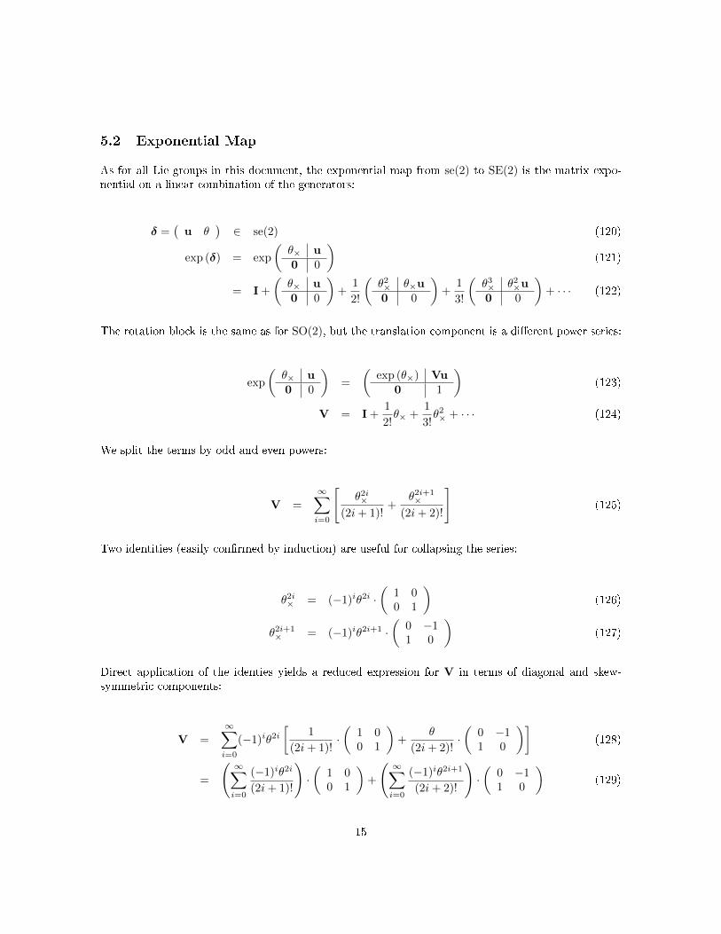
5.2 Exponential Map

As for all Lie groups in this document, the exponential map from se(2) to SE(2) is the matrix expo-nential on a linear combination of the generators:

δ =(

u θ)∈ se(2) (120)

exp (δ) = exp

(θ× u0 0

)(121)

= I +

(θ× u0 0

)+

1

2!

(θ2× θ×u0 0

)+

1

3!

(θ3× θ2×u0 0

)+ · · · (122)

The rotation block is the same as for SO(2), but the translation component is a di�erent power series:

exp

(θ× u0 0

)=

(exp (θ×) Vu

0 1

)(123)

V = I +1

2!θ× +

1

3!θ2× + · · · (124)

We split the terms by odd and even powers:

V =

∞∑i=0

[θ2i×

(2i+ 1)!+

θ2i+1×

(2i+ 2)!

](125)

Two identities (easily con�rmed by induction) are useful for collapsing the series:

θ2i× = (−1)iθ2i ·(

1 00 1

)(126)

θ2i+1× = (−1)iθ2i+1 ·

(0 −11 0

)(127)

Direct application of the identies yields a reduced expression for V in terms of diagonal and skew-symmetric components:

V =

∞∑i=0

(−1)iθ2i[

1

(2i+ 1)!·(

1 00 1

)+

θ

(2i+ 2)!·(

0 −11 0

)](128)

=

( ∞∑i=0

(−1)iθ2i

(2i+ 1)!

)·(

1 00 1

)+

( ∞∑i=0

(−1)iθ2i+1

(2i+ 2)!

)·(

0 −11 0

)(129)

15

The coe�cients can be identi�ed with Taylor expansions:

V =

(1− θ2

3!+θ4

5!+ · · ·

)·(

1 00 1

)+

(θ

2!− θ3

4!+θ5

6!+ · · ·

)·(

0 −11 0

)(130)

=

(sin θ

θ

)·(

1 00 1

)+

(1− cos θ

θ

)·(

0 −11 0

)(131)

=1

θ·(

sin θ −(1− cos θ)1− cos θ sin θ

)(132)

For implementation purposes, Taylor expansions should be used for V when θ is small.

The ln() function on SE(2) can be implemented by �rst recovering θ = ln(R) as shown in Eq. 108,then solving Vu = t for u in closed form:

A ≡ sin θ

θ(133)

B ≡ 1− cos θ

θ(134)

V−1 =1

A2 +B2

(A B−B A

)(135)

ln

(R t0 1

)=

(V−1 · t

θ

)∈ se(2) (136)

5.3 Adjoint

The adjoint in SE(2) is computed from the generators:

δ =(

u θ)T ∈ se(2), C =

(R t0 1

)∈SE(2) (137)

AdjC · δ = C ·

(3∑i=1

δiGi

)· C−1 (138)

=

Ru + θ

(t2−t1

)θ

(139)

=⇒ AdjC =

Rt2−t1

0 1

∈ R3×3 (140)

Note that moving a tangent vector via the adjoint mixes the rotation component into the translationcomponent.

16

6 Sim(3): Similarity Transformations in 3D space

6.1 Representation

Similarity transformations are combinations of rigid transformation and scaling. The group of similar-ity transforms in 3D space, Sim(3), has a nearly identical representation to SE(3), with an additionalscale factor:

R ∈ SO(3), t ∈ R3, s ∈ R (141)

T =

(R t0 s−1

)∈ Sim(3) (142)

Again, group operations map are isomorphic with matrix operations:

T1, T2 ∈ Sim(3) (143)

T1 · T2 =

(R1 t10 s−11

)·(

R2 t20 s−12

)(144)

=

(R1R2 R1t2 + s−12 t1

0 (s1 · s2)−1)

(145)

T−11 =

(RT

1 −s1RT1 t

0 s1

)(146)

The group action on 3D points also encodes scaling by s:

x =(x y z w

)T ∈ RP3 (λx ' x ∀λ ∈ R)

T · x =

(R t0 s−1

)· x (147)

=

(R(x y z

)T+ wt

s−1w

)(148)

'

(s(R(x y z

)T+ wt

)w

)(149)

In the typical case with w = 1, this corresponds to rigid transformation followed by scaling.

The generators of the Lie algebra sim(3) are identical to those of se(3) (Eq. 65), with the addition ofa generator corresponding to scale change:

G7 =

0 0 0 00 0 0 00 0 0 00 0 0 −1

(150)

17

An element of sim(3) is represented by multiples of the generators:

(u ω λ

)T ∈ R7 (151)

u1G1 + u2G2 + u3G3 + ω1G4 + ω2G5 + ω3G6 + λG7 ∈ sim(3) (152)

For convenience, we write(

u ω λ)T ∈ sim(3), with multiplication against the generators implied.

6.2 Exponential Map

As above, the exponential map from sim(3) to Sim(3) is the matrix exponential on a linear combinationof the generators:

δ =(

u ω λ)∈ sim(3) (153)

exp (δ) = exp

(ω× u0 −λ

)(154)

= I +

(ω× u0 λ

)+

1

2!

(ω2× ω×u− λu

0 λ2

)+

1

3!

(ω3× ω2

×u− λω×u + λ2u0 −λ3

)+ · · ·(155)

The series is similar to that for se(3), but now rotation, translation and scale are being interleavedin�nitesimally. The rotation and scale components of the exponential are immediately clear, but thetranslation component involves the mixing of the three. We can write out the series for the translationmultiplier:

exp

(ω× u0 0

)=

(exp (ω×) Vu

0 exp (−λ)

)(156)

V =

∞∑n=0

n∑k=0

ωn−k× (−λ)k

(n+ 1)!(157)

=

∞∑k=0

∞∑n=k

ωn−k× (−λ)k

(n+ 1)!(158)

=

∞∑k=0

∞∑j=0

ωj× (−λ)k

(j + k + 1)!(159)

Again letting θ2 = ωTω, and using the identity from Eq. 9, we partition the terms into odd and evenpowers of ω×, and factor:

V =

( ∞∑k=0

(−λ)k

(k + 1)!

)I +

∞∑k=0

(−λ)k∞∑i=0

[ω2i+1×

(2i+ k + 2)!+

ω2i+2×

(2i+ k + 3)!

](160)

=

( ∞∑k=0

(−λ)k

(k + 1)!

)I +

( ∞∑k=0

∞∑i=0

(−1)iθ2i (−λ)k

(2i+ k + 2)!

)ω× +

( ∞∑k=0

∞∑i=0

(−1)iθ2i (−λ)k

(2i+ k + 3)!

)ω2× (161)

18

The �rst coe�cient is easily identi�ed as a Taylor series, leaving the other two coe�cients to beanalyzed:

V = AI +Bω× + Cω2× (162)

A =1− exp (−λ)

λ(163)

B =

∞∑k=0

∞∑i=0

(−1)iθ2i (−λ)k

(2i+ k + 2)!(164)

C =

∞∑k=0

∞∑i=0

(−1)iθ2i (−λ)k

(2i+ k + 3)!(165)

Consider coe�cient B:

B =

∞∑k=0

∞∑i=0

(−1)iθ2i (−λ)k

(2i+ k + 2)!(166)

=

∞∑i=0

[(−1)iθ2i

∞∑k=0

(−λ)k

(2i+ k + 2)!

](167)

=

∞∑i=0

[(−1)iθ2i

λ2i

∞∑k=0

(−λ)2i+k

(2i+ k + 2)!

](168)

=

∞∑i=0

[(−1)iθ2i

λ2i

∞∑m=2i

(−λ)m

(m+ 2)!

](169)

=

∞∑i=0

((−1)iθ2i

λ2i

[ ∞∑m=0

(−λ)m

(m+ 2)!−

2i−1∑m=0

(−λ)m

(m+ 2)!

])(170)

=∞∑i=0

((−1)iθ2i

λ2i

[ ∞∑m=0

(−λ)m

(m+ 2)!

])−∞∑i=0

((−1)iθ2i

λ2i

2i−1∑m=0

(−λ)m

(m+ 2)!

)(171)

Manipulating the second term yields a more useful form:

19

L ≡∞∑i=0

((−1)iθ2i

λ2i

[ ∞∑m=0

(−λ)m

(m+ 2)!

])(172)

B = L−∞∑i=0

((−1)iθ2i

λ2i

2i−1∑m=0

(−λ)m

(m+ 2)!

)(173)

= L−∞∑i=0

((−1)iθ2i

λ2i

i−1∑p=0

[(−λ)2p

(2p+ 2)!+

(−λ)2p+1

(2p+ 3)!

])(174)

= L−∞∑i=0

((−1)iθ2i

λ2i

i−1∑p=0

(−λ)2p[

1

(2p+ 2)!− λ

(2p+ 3)!

])(175)

= L−∞∑p<i

((−1)iθ2i

λ2i(−λ)2p

[1

(2p+ 2)!− λ

(2p+ 3)!

])(176)

= L−∞∑p<i

((−1)iθ2i

λ2(i−p)

[1

(2p+ 2)!− λ

(2p+ 3)!

])(177)

= L−∞∑p=0

∞∑q=1

((−1)qθ2q

λ2q

[(−1)pθ2p

(2p+ 2)!− λ

((−1)pθ2p

(2p+ 3)!

)])(178)

= L−

( ∞∑q=1

(−1)qθ2q

λ2q

)( ∞∑p=0

[(−1)pθ2p

(2p+ 2)!− λ

((−1)pθ2p

(2p+ 3)!

)])(179)

=

(∑∞i=0

(−1)iθ2i

λ2i

)(∑∞m=0

(−λ)m

(m+ 2)!

)−(∑∞

q=0

(−1)qθ2q

λ2q− 1

)(∑∞p=0

[(−1)pθ2p

(2p+ 2)!− λ

((−1)pθ2p

(2p+ 3)!

)]) (180)

Relabel the factors:

B = α · β − (α− 1) · γ (181)

= α · (β − γ) + γ (182)

α ≡∞∑i=0

(−1)iθ2i

λ2i(183)

β ≡∞∑m=0

(−λ)m

(m+ 2)!(184)

γ ≡∞∑p=0

[(−1)pθ2p

(2p+ 2)!− λ

((−1)pθ2p

(2p+ 3)!

)](185)

20

The factors are then recognised as Taylor series:

α =λ2

λ2 + θ2(186)

β =exp (−λ)− 1 + λ

λ2(187)

γ =1− cos θ

θ2− λ

(θ − sin θ

θ3

)(188)

By similar algebra, a formula for coe�cient C can be derived from Eq. 165:

C = α · (µ− ν) + ν (189)

µ =1− λ+ 1

2λ2 − exp (−λ)λ2

(190)

ν =θ − sin θ

θ3− λ

(cos θ − 1 + θ2

2

θ4

)(191)

Combining these results gives a closed-form exponential map for sim(3):

21

(u ω λ

)T ∈ sim(3) (192)

θ2 = ωTω (193)

X =sin θ

θ(194)

Y =1− cos θ

θ2(195)

Z =1−Xθ2

(196)

W =12 − Yθ2

(197)

α =λ2

λ2 + θ2(198)

β =exp (−λ)− 1 + λ

λ2(199)

γ = Y − λZ (200)

µ =1− λ+ 1

2λ2 − exp (−λ)λ2

(201)

ν = Z − λW (202)

A =1− exp (−λ)

λ(203)

B = α · (β − γ) + γ (204)

C = α · (µ− ν) + ν (205)

R = I + aω× + bω2× (206)

V = AI +Bω× + Cω2× (207)

exp

uωλ

=

(R Vu0 exp (−λ)

)(208)

Again, Taylor expansions should be used when λ2 or θ2 is small. The ln() function can be implementedby �rst recovering ω and λ, constructing V, and then solving for u (as in the SE(3) case).

6.3 Adjoint

The adjoint is computed from a linear combination of the generators:

22

δ =(

u ω λ)T ∈ sim(3), T =

(R t0 s−1

)∈Sim(3) (209)

T · exp (δ) = exp (AdjT · δ) · Texp (AdjT · δ) = T · exp (δ) · T−1 (210)

AdjT · δ = T ·

(7∑i=1

δiGi

)· T−1 (211)

=

s (Ru + t×Rω − st)Rω−λ

(212)

=⇒ AdjT =

sR st×R −st0 R 00 0 1

∈ R7×7 (213)

7 Interpolation

Consider a Lie group G, with two elements a, b ∈ G. We would like to interpolate between theseelements, according to a parameter t ∈ [0, 1]. De�ne a function that will perform the interpolation:

f : G×G× R → G (214)

f (a, b, 0) = a (215)

f (a, b, 1) = b (216)

The function is de�ned by transforming the interpolation operation into the tangent space, perform-ing the linear combination there, and then transforming the resulting tangent vector back onto themanifold. First consider the group element that takes a to b:

d ≡ b · a−1 ∈ G (217)

d · a = b (218)

Now compute the corresponding Lie algebra vector and scale it in the tangent space:

d(t) = t · ln (d) (219)

Then transform back into the manifold using the exponential map, yielding a �partial� transformation:

dt = exp (d(t)) (220)

Combining these three steps gives a de�nition for f :

23

f(a, b, t) = dt · a (221)

= exp(t · ln

(b · a−1

))· a (222)

Note that the result is always on the manifold, due to the properties of the exponential map. Noprojection or coercion is required. Furthermore, the linear transformation in the tangent space cor-responds to moving along a geodesic of the manifold. So the interpolation always moves along the�shortest� transformation in the Lie group.

8 Uncertain Transformations

8.1 Sampling

Consider a Lie group G and its associated Lie algebra vector space g, with k degrees of freedom. Wewish to represent Gaussian distributions over transformations in this group. Each such distributionhas a mean transformation, µ ∈ G, and a covariance matrix Σ ∈ Rk×k. The algebra corresponds totangent vectors around the identity element of the group. Thus, it is natural to express a sample xfrom the desired distribution in terms of a sample δ drawn from a zero-mean Gaussian and the meantransformation µ:

δ ∈ N (0;Σ) (223)

x = exp (δ) · µ (224)

8.2 Transforming

This formulation allows convenient transformations of distributions through other group elements usingthe adjoint. Consider x, y ∈ G, and the distribution (x,Σ) with mean x. Consider y · x̃, where x̃ is asample drawn from (x,Σ):

x̃ = exp (δ) · x (225)

y · x̃ = y · exp (δ) · x (226)

= exp(Adjyδ

)· y · x (227)

By the de�nition of covariance,

Σ = E[δ · δT

](228)

Given a linear transformation L, by linearity of expectation we have:

E[(Lδ) · (Lδ)T

]= E

[L · δ · δT · LT

](229)

= L · E[δ · δT

]· LT (230)

= L ·Σ · LT (231)

24

So we can express the parameters of the transformed distribution:

y · x̃ ∈ N(y · x; Adjy ·Σ ·AdjTy

)(232)

Thus the mean of the transformed distribution is the transformed mean, and the covariance is mappedlinearly by the adjoint.

8.3 Distribution of Inverse

Similarly, the distribution of the inverse transformation is easily computed:

z̃ ≡ x̃−1 (233)

= x−1 · exp (−δ) (234)

= exp (−Adjx−1δ) · x−1 (235)

z̃ ∈ N(x−1; Adjx−1 ·Σ ·AdjTx−1

)(236)

8.4 Projection through Group Actions

Because the covariance is expressed in terms of tangent vectors (exponentiated and multiplied onthe left-hand side), all the Jacobians given in the group descriptions above can be used to transformcovariance (or information) matrices through arbitrary mappings.

8.5 Computing Moments from Samples

Given a Lie group G (with algebra g) and a set of N samples xi ∈ G, we can estimate the mean andcovariance iteratively. First, any of the samples provides an initial guess for the mean:

µ0 ← x0 (237)

Then, new estimates of the mean and covariance can be computed in terms of deviations in the tangentspace:

vi,k ≡ ln(xi · µ−1k

)(238)

Σk ← 1

N

∑i

[vi,k · vTi,k

](239)

µk+1 ← exp

(1

N

∑i

vi,k

)· µk (240)

Iterating these updates should rapidly converge (typically in two or three iterations). Replacing the

factor1

Nwith

1

N − 1in Eq. 239 yields an unbiased estimate of the covariance.

25